university of birmingham evaluating the impact of land-use
TRANSCRIPT
University of Birmingham
Evaluating the impact of land-use density and mixon spatiotemporal urban activity patterns: anexploratory study using mobile phone dataJacobs-Crisioni, Chris; Rietveld, Piet; Koomen, Eric; Tranos, Emmanouil
DOI:10.1068/a130309p
License:None: All rights reserved
Document VersionPeer reviewed version
Citation for published version (Harvard):Jacobs-Crisioni, C, Rietveld, P, Koomen, E & Tranos, E 2014, 'Evaluating the impact of land-use density andmix on spatiotemporal urban activity patterns: an exploratory study using mobile phone data', Environment andPlanning A, vol. 46, no. 11, pp. 2769-2785. https://doi.org/10.1068/a130309p
Link to publication on Research at Birmingham portal
Publisher Rights Statement:Final Version of Record available online at: http://dx.doi.org/10.1068/a130309p
Checked November 2015
General rightsUnless a licence is specified above, all rights (including copyright and moral rights) in this document are retained by the authors and/or thecopyright holders. The express permission of the copyright holder must be obtained for any use of this material other than for purposespermitted by law.
•Users may freely distribute the URL that is used to identify this publication.•Users may download and/or print one copy of the publication from the University of Birmingham research portal for the purpose of privatestudy or non-commercial research.•User may use extracts from the document in line with the concept of ‘fair dealing’ under the Copyright, Designs and Patents Act 1988 (?)•Users may not further distribute the material nor use it for the purposes of commercial gain.
Where a licence is displayed above, please note the terms and conditions of the licence govern your use of this document.
When citing, please reference the published version.
Take down policyWhile the University of Birmingham exercises care and attention in making items available there are rare occasions when an item has beenuploaded in error or has been deemed to be commercially or otherwise sensitive.
If you believe that this is the case for this document, please contact [email protected] providing details and we will remove access tothe work immediately and investigate.
Download date: 01. Dec. 2021

Evaluating the impact of land‐use density and mix on spatiotemporal urban activity patterns: an
exploratory study using mobile phone data
Chris Jacobs‐Crisioni MSc1 (corresponding author) [email protected]; + 31 6 383 148 22 Prof. Dr. Piet Rietveld2 [email protected] Dr. Eric Koomen2 [email protected] Dr. Emmanouil Tranos3 [email protected] 1 European Commission, Joint Research Centre, Institute for Environment and Sustainability, Land Management and Natural Hazards Unit, Via E. Fermi, 2749, 21027 Ispra (Va), Italy 2 Faculty of Economics and Business Administration, VU University Amsterdam Boelelaan 1105 1081HV Amsterdam 3School of Geography, Earth and Environmental Sciences (GEES) University of Birmingham Edgbaston, Birmingham, B15 2TT, UK
Acknowledgements
We wish to thank the Dutch Ministry of Infrastructure and the Environment for providing phone
usage data, John Steenbruggen and Ronnie Lassche for their assistance in providing data, and
Maarten Hilferink and Martin van der Beek of ObjectVision for their assistance in using the
GeoDMS framework. This research was funded by the research programme Urban Regions in the
Delta, part of the ‘Verbinding Duurzame Steden’ programme of the Netherlands Organisation for
Scientific Research. The preparation of this paper has been overshadowed by Piet Rietveld’s death
in November 2013. His thoughts, ideas and critiques contributed greatly to this article, and with
sadness we dedicate this work in memory of him.

1
Evaluating the impact of land-use density and mix on spatiotemporal urban activity patterns:
an exploratory study using mobile phone data
ABSTRACT: Dense and mixed land-use configurations are assumed to encourage high and
prolonged activity levels, which in turn are considered to be important for the condition of urban
neighbourhoods. We used mobile phone usage data recorded in Amsterdam, the Netherlands,
as a proxy for urban activity to test if the density in different forms of urban land use increases
the level of activity in urban areas, and if mixed land uses can prolong high levels of activity in
an area. Our results indicate that higher densities correspond with higher activity levels, mixed
land uses do indeed diversify urban activity dynamics and colocating particular land uses
prolongs high activity levels in the evening hours. We proceed to demonstrate that mixed
activity provisions and high urban activity levels coincide with urban neighbourhoods that are
considered attractive places in which to live and work, while lower activity levels and markedly
low activity mixes coincide with neighbourhoods that are considered disadvantaged.
KEYWORDS: Mobile phone usage, land-use density, land-use mix

2
1 Introduction
Since at least the 1990s there has been increasing political support for planning approaches
that aim to achieve dense and mixed urban land-use patterns (Grant, 2002; Stead and
Hoppenbrouwer, 2004; Vreeker et al, 2004). The desired land-use patterns are expected to
improve urban vitality, safety and quality of life, and make cities more sustainable and
attractive (Coupland, 1997). As Hoppenbrouwer and Louw (2005) point out, many of the
arguments used in favour of dense and mixed land use are still based on Jacobs (1962), who
argued that such land-use configurations increase and prolong activity intensities in a
neighbourhood. In her seminal work Jacobs observed that (1) safe and pleasant public spaces
are the distinguishing characteristic of vibrant urban neighbourhoods, and (2) public spaces in
large cities have very specific requirements in order to function effectively. Jacobs argued that
in the public spaces of vibrant urban neighbourhoods an ad hoc social structure exists that
maintains order (i.e., provides natural animation; Petterson, 1997) and stimulates residents to
watch or engage in the daily events in public space (i.e., provides natural entertainment;
Montgomery, 1995). Such a social structure, upheld by residents and strangers passing by,
would emerge naturally when diverse people are almost continuously present on a
neighbourhood’s streets. Jacobs (1962) argued that in order to have sufficient, continuous
human presence in public space, urban areas need to support activities with sufficient intensity
and diversity in terms of temporal participation patterns, so that pedestrians populate the
streets for substantial parts of the day.
Dense land-use configurations are expected to contribute to vibrant neighbourhoods by
increasing urban activity intensities. One may argue that increasing land-use densities might

3
instead lead to unwanted crowding effects, but perceived crowding and available physical
space per capita are often unrelated (Bonnes et al, 1991; Fischer et al, 1975) and perceived
crowding depends much more on other factors (Chan, 1999). Mixed land-use configurations are
expected to extend activity intensities, and diversify the `ebbs and tides’ of people coming and
going into an area to participate in the activities provided (Roberts and Lloyd-Jones, 1997: p
153). Mixed land use is furthermore presumed to generate multiplier effects that help extend
activity intensities by retaining people in an area that they initially visited for another activity
(Jacobs, 1962; Rodenburg et al, 2003).
Contemporary planners have adopted Jacobs’s ideas, and found that encouraging higher and
extended activity intensities by developing dense and mixed land-use configurations can have
disappointing results. This is particularly unfortunate because dense and mixed developments
are often very difficult to achieve (for experiences with establishing such developments, see
Coupland, 1997; Grant, 2002; Majoor, 2006; Petterson, 1997; Rowley, 1996). There are
reasonable arguments why developing denser and more diverse land uses might not contribute
to neighbourhood success at all. First and foremost, there is no proven impact of the physical
environment on behaviour, as emphasised by Gans (1991). Another problem is that the
demand for the specific type of urban environments at which densification and mixed
development aim is presumably limited, and as Gans notes, may only stem from the upper
middle class and young urban professionals. Furthermore, existing social environments in the
city may already have established a hierarchy of preferred places to which their events and
activities are closely tied (Currid and Williams, 2010). If such environments are indeed tied to
particular places, the development of new activity spaces is successful only if the new spaces

4
provide additional facilities that do not compete with the established hierarchy, or if a new type
of social environment emerges.
Clearly more work is needed to find if dense and mixed land-use patterns can indeed foster
vibrant neighbourhoods. Besides Jacobs’s work, only a few case studies have linked land-use
density to desirable aspects of vibrant neighbourhoods such as attractiveness (Gadet et al,
2006) and low crime rates (Coleman, 1985; Petterson, 1997). These studies neither yield
conclusive evidence on this subject, nor address the overall link between land-use intensity and
activity levels. A data source that has recently become available – mobile phone usage data – is
used in this article to evaluate empirically the potential impact of dense and mixed land use on
urban activity intensities. We used phone usage densities as a proxy for urban activity intensity
and, for each hour of the day, statistically analysed the link between, on the one hand, activity
levels and, on the other hand, the densities of various land uses and the interactions between
colocated land uses. We did so in order to verify if higher land-use densities correspond with
higher activity intensities, if the activities associated with those land uses have diverse temporal
patterns and if multiplier effects exist between particular activities supporting each other when
colocated. Subsequently, to test if high and extended activity intensities do indeed coincide
with favourable neighbourhood conditions, we compared observed and modelled phone usage
densities in (1) districts that experts consider successful in attracting members of the creative
class, and (2) districts that according to experts are accumulating persistent social, economic
and physical problems. We must emphasise here that we explored the coincidence of activity
patterns and neighbourhood conditions, but have not verified the causal link proposed by
Jacobs (1962) between activity intensities and neighbourhood success. In fact, there are many

5
factors affecting the neighbourhood conditions analysed, and a thorough study of the
mechanics that govern those conditions is well beyond the scope of this paper. In the following
section we expand on the data and methods used; in the subsequent sections we demonstrate
our evidence in favour of dense and mixed land-use configurations.
2 Data, methods and limitations
For this study, mobile phone data recorded between January 2008 and November 2010 has
been obtained from KPN, one of the main telecommunication service providers in the
Netherlands. Such mobile phone usage data have been emphasised as particularly suitable for
urban analysis (Ratti et al, 2006). Recent contributions using such data have explored seasonal
migration and the composition of traffic flows in Estonia (Silm and Ahas, 2010 and Järv et al,
2012, respectively); linkages between phone usage and city characteristics in Rome (Reades et
al, 2009) and the locations of personal `anchor’ activity bases in Estonia (Ahas et al, 2010: p 4).
The activity patterns that Ahas et al derived are very similar to the spatial distribution of the
population as observed in census data, and the authors therefore concluded that mobile phone
usage is suitable for studying urban activities. The present study also presumes such a link
between human activity patterns and mobile phone usage.
One important issue arises regarding privacy considerations that relate to the storing and
analysing of personal communications, such as in the data used. The data obtained contain only
aggregate usage statistics per mobile phone cell, and characteristics of the mobile phone users
were not recorded. Thus, the data cannot be used to identify individual users and we therefore
assume that privacy concerns are not problematic for this study. We elaborate on the mobile

6
phone usage data, the modelled linkages with land-use and activity patterns and some
methodological limitations in the next sections, after addressing the study area. A scheme of
this paper’s approach can be found in Figure 1.
Figure 1: Conceptual scheme for this paper’s analyses, and the operationalisation of the main variables applied.
The city of Amsterdam in the Netherlands, entailing considerable geographical differences in
urban density and in the degree of land-use mix, will serve as a case. Because the mixed-use
literature seems to concentrate on land-use mixing in residential areas (see, for example,
Cervero, 1996; Jacobs, 1962), we also limit our study to areas that have a residential purpose.
We therefore only use data from antennas within urban districts with a population density of at
least 200 inhabitants per km2. Note that Amsterdam’s average population density is 3,800
inhabitants per km2. Only rural and dominantly industrial areas on the outskirts of the city are
Multiplier effects Combinations of land uses in area
Spatiotemporal activity patterns Mobile phone activity as a proxy
Living and working Inhabitant densities Share of land used for businesses
Amenities for residents and visitors Share of land used for shops Share of land used for meeting places Transport availability Tourist squares
Neighbourhood conditions Areas deemed attractive vs. areas deemed problematic
7
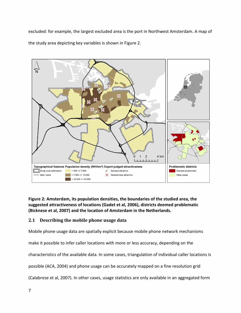
excluded: for example, the largest excluded area is the port in Northwest Amsterdam. A map of
the study area depicting key variables is shown in Figure 2.
Figure 2: Amsterdam, its population densities, the boundaries of the studied area, the suggested attractiveness of locations (Gadet et al, 2006), districts deemed problematic (Bicknese et al, 2007) and the location of Amsterdam in the Netherlands.
2.1 Describing the mobile phone usage data
Mobile phone usage data are spatially explicit because mobile phone network mechanisms
make it possible to infer caller locations with more or less accuracy, depending on the
characteristics of the available data. In some cases, triangulation of individual caller locations is
possible (ACA, 2004) and phone usage can be accurately mapped on a fine resolution grid
(Calabrese et al, 2007). In other cases, usage statistics are only available in an aggregated form
8
per antenna, and then attributed to portions of space where callers using that antenna are
presumed to be. Examples are cases in which mobile phone usage has been interpolated into a
continuous surface (Ratti et al, 2006) or attributed to superimposed catchment areas (Ahas et
al, 2010). The mobile phone usage data provided for this paper are attributed to a similar
network-specific zonal topography named `best-serving cells’. These cells are the results of
sampling and subsequently mapping which antennas provide the best connection and they
represent the areas that are usually connected to a particular antenna. Temporary changes in
the network structure are not taken into account. This topology is created by the mobile phone
service provider, who unfortunately does not allow disclosure of its mapping work.
Phone usage on the provider’s network in the Amsterdam region has been made available for
this study, save a number of months for which data are missing. There is a distinction between
mobile phone usage data in which all phones connected to the network are recorded and data
in which only phones that are using the network are recorded. The obtained phone usage data
describe aggregate use: for example, the number of newly initiated calls per mobile phone cell
per hour per day. Figure 3 indicates that, on average, more than 2 million phone calls were
made over the 2G network each day in the observed period in the Amsterdam region.
We observed itY as the average number of newly initiated mobile phone calls1 per hour (t)
through antennas (i) per square kilometre of the best serving cell. The average number of new
1 Other studies (Ratti et al, 2006; Reades et al, 2009) use bandwidth consumption (‘Erlang’). We prefer newly
initiated phone calls as an approximation of human presence because we expect that this indicator is less biassed towards activities that accommodate a disproportional amount of bandwidth. Furthermore, we expect that the portion of calls related to transportation is lower in new phone calls because we assume that people who are travelling (by car or by bicycle) are less likely to initiate a mobile phone call. This is useful because we want to focus on the presence of people in a place, rather than the flows of people in space.

9
calls has been computed here as the average number of newly initiated phone calls per hour on
all recorded working days from January to June 2010. Those data were used in 24 cross-
sectional regressions, one for each hour of the day. The analysis centres on observations from
that period because they are reasonably close to the land-use data that are only available for
2012, while due to network changes, results from after June 2010 are structurally different (this
is also discussed in the following section). We expected that because of the averaged nature of
the dependent variable, sporadically occurring events such as the Queen’s Day national holiday
would not have a substantial effect on our results. To test the robustness of our findings, we
have repeated our analyses with data for all available months.
Figure 3: Monthly averages of new calls per day via the 2G network. Data for some intermittent months were not provided. The decrease in phone usage over time is caused by an increasing proportion of calls carried through the 3G network.
Some pre-processing has been necessary to use the data. The data originally comprised phone
usage statistics from two frequencies (900 and 1800 MHz), of which the antennas have
0
2
4
Mill
ion
s o
f p
ho
ne
cal
ls in
th
e s
tud
y ar
ea

10
overlapping but differently sized and shaped catchment areas. Network mechanisms such as
capacity balancing mean that mobile phone usage statistics of the two frequencies are
inextricably related, and therefore need to be analysed together. The data have therefore been
integrated into summed statistics for the smaller 900 MHz frequency cells that handle the
largest proportion of network traffic. Phone usage statistics of the 1800 MHz frequency have
been disaggregated to that topology based on proportions of the overlapping areas.2 When
mapped, the data capture substantial temporal and geographical differences in activity levels
(see Figures 4 and 5).
Figure 4: Fifth percentile (perc.), 95th percentile and average number of new calls over the course of the day per km2.
2 Thus, if 1% of one 1800 MHz area overlaps one particular 900 MHz cell, 1% of traffic recorded in the 1800 MHz
area is attributed to that 900 MHz cell, and so on.
0
1,000
2,000
3,000
0.00 4.00 8.00 12.00 16.00 20.00 24.00
Ave
rage
ne
w c
alls
pe
r km
2
Time of day
95th percentile
Average
5th percentile

11
Figure 5: Spatial distribution of new calls per km2 in Amsterdam and its environs (workday averages 2008–2010). Dark black lines indicate motorways. The study area is gray with a darker outline, except for the white areas within it, which indicate missing data.
2.2 Explaining spatiotemporal patterns in mobile phone usage
We assume that the time and location of mobile phone usage is related to general human
activity patterns and the location where these activities take place. The temporal activity
patterns in the Netherlands have been rather stable since at least the 1970s (De Haan et al,
2004). The average weekday participation rates of the Dutch population in a selection of
activities are shown in Figure 6. These national participation rates are likely to differ from the
participation rates of the population studied here, but a comparison with Figure 4 shows a clear
relation between overall participation in activities and mobile phone usage. From Figure 6 we

12
can hypothesise that, given the dominant participation rates for working and leisure activities
(whether at home or outdoors) throughout the day, these activities will likely have the largest
impact on mobile phone usage densities.
Figure 6: Temporal variation in a selection of weekday activities by percentage of Dutch people older than 12 years of age who participate in them. Sources: Breedveld et al, 2006; Cloïn et al, 2011.
The activities distinguished in Figure 6 are likely to take place at different locations, so we
propose an explanatory framework that combines the basic activities with a spatial
representation of the locations where these activities are concentrated. This spatial context is
offered by detailed land-use maps that highlight the locations where working, shopping and
leisure activities at home and outdoors are concentrated. In this explanatory framework we
fitted mobile phone usage densities on different land-use types that can be associated with the
main types of human activity (Table 1). This approach allows us to explain spatiotemporal
variation in mobile phone usage and provides insight into the importance of land-use density in
generating the concentrations of people active in the urban environment. By specifically looking
0
25
50
75
100
0.00 4.00 8.00 12.00 16.00 20.00 24.00
Act
ivit
y p
arti
cip
atio
n %
Time of day
Working
Shopping
Sleeping
Spare time and eating

13
at the impact of different combinations of land-use types, we are also able to assess the
importance of land-use mixing in generating urban activity.
Table 1: Land-use types and their definition.
Leisure at home Inhabitants per square kilometre, reflecting leisure opportunities at home
Working Proportion of area used by factories, offices and schools, reflecting working opportunities
Shops Proportion of area used by shops, reflecting shopping opportunities
Outdoor leisure Proportion of area used by various building types dedicated to social meetings such as cafés, restaurants, churches, conference rooms and discotheques, reflecting outdoor leisure opportunities
The land-use data are obtained from two data sources. Activities at home are observed by
means of inhabitant densities per km2, aggregated to the best serving cells from approximately
18,000 postcodes in the study area (Statistics Netherlands, 2006). Working, shopping and social
activities are approximated by means of land-use densities that are computed as the summed
sizes of partial or total building footprints designated to a particular land use versus the total
area of the catchment area. The building footprints and designations are derived from detailed
building footprint data (Kadaster, 2013) in which the land-use designations of all independent
units (e.g., apartments or offices) within all buildings in the Netherlands are recorded. To
compute land-use densities from those independent units, the total areal footprint of buildings
is distributed equally over all the independent units that a building contains, and the total
footprints of those independent units are summed per land-use type per mobile phone cell.
Thus, if a building with a 60 m2 footprint contains three independent units, of which two are
designated to land-use A and one to land-use B, 40 m2 of the building’s footprint is attributed to

14
A and 20 m2 is attributed to B. We must acknowledge that information on floor space per
independent unit is not included in this data, which may possibly skew the density figures
because building heights will be higher in particular areas of the city. However, the data applied
still provide a much more detailed description of land uses than the remotely sensed data that
are often used in land-use studies, and we believe that the data used are a workable alternative
as long as more accurate sources such as information on floor space are unavailable.
2.3 Methodological limitations
The data used impose a number of important limitations. A first limitation is that some
activities likely encourage phone use more than other activities. Thus, mobile phone usage is
presumably biased towards certain activities. We assumed this is not problematic because all
activities are captured to some degree in the modelling exercise, which is sufficient for this
study. Another limitation is that, while neighbourhoods supposedly need pedestrians, the data
used does not discern callers that are outdoors or indoors. We thus have to assume that higher
activity intensities and more diverse temporal activity patterns lead to more pedestrian activity.
This likely holds true in Amsterdam, a city that actively discourages private car use.
Another concern related to the used mobile phone data is that only phone usage data from the
so-called 2G network have been obtained, while during the observed period, mobile phone
services were provided in the Amsterdam region by both second generation (2G) and third
generation (3G) network technology. Especially in 2010 a substantial share of mobile phone
usage, 36%, has used the 3G network (see KPN, 2011), which causes the previously mentioned
shift in results after June 2010. Nevertheless, the majority of phone calls used the 2G network

15
even in 2010, and we therefore believe that the shift in traffic from 2G to 3G has not severely
affected our findings.
Other limitations are related to the spatial nature of phone usage data. The zones used cover
an area of 0.5 km2 on average, and are thus of a relatively fine spatial resolution, but still much
larger than the streets and blocks analysed in other studies of land-use mixing (Hoppenbrouwer
and Louw, 2005; Jacobs, 1962; Rodenburg et al, 2003). Because of the fixed resolution of the
available data, the detail of those previous studies cannot be repeated here, and we cannot
account for relevant aspects of urban land-use configuration such as street connectivity and
grain size. We nevertheless expect that the spatial and temporal comprehensiveness of the
data used is valuable for understanding the effects of land-use density and mix on activity
levels. Another difficulty of using data based on presumed antenna catchment areas is that,
because the antenna providing the best connection to one place may vary with temporal
conditions, changes in the built environment or even chance reflections in water, the link
between caller location and the connecting antenna is of a stochastic rather than deterministic
nature. Thus, callers are often falsely attributed to neighbouring catchment areas (see also
Ahas et al, 2010). We presume that this is one cause of spatial autocorrelation in the data. To
overcome spatial autocorrelation in the data, a spatial error model is applied (see Anselin,
2001; LeSage and Fischer, 2008). Furthermore, the use of discretely bordered areal units brings
forth the modifiable areal unit problem (Openshaw, 1984), of which the differences in areal
sizes of zones in particular can bias statistical findings (Arbia, 1989). These biases can in part be
overcome by normalising observations by average cell size (see Jacobs-Crisioni et al, 2014, for a
recent overview), which we do by means of equation (1):

16
(
∑ )
(1)
where weight S is computed for each cell i by means of geographical area A.
3 The impact of land-use density and mix on hourly urban activity patterns
To estimate the impact of land-use densities and mixes on mobile phone usage in zones (i = 1,
2, ..., 362), we fit the spatial error model shown in equation (2) repeatedly on the selected time
frame’s averaged new call densities for one hour of the day (t = 0, 1, … , 23):
( ) ( )
( ) ( )
,
(2)
in which the observations i are additionally weighted with the weighting values discussed in
section 2.1. In our approach the impacts of densities of inhabitants (INH), businesses (BUS),
shops (SH) and meeting places (MP) on phone usage levels are estimated. Furthermore,
potential interaction effects between different land uses are captured. We are aware that land-
use mix is an ambiguous concept which in all cases has to do with land-use diversity within
cities, but which can occur on varying scales and with varying impacts on activity dynamics
(Rowley, 1996). Unsurprisingly, there are many methods to measure degrees of land-use
mixing; for an overview, we refer to Manaugh and Kreider (2013). We model land-use mixes by
means of interaction effects between the densities of particular land uses colocated within one
areal unit. On a side note, aggregate indicators of land-use mix based on the Herfindahl
concentration index have also been tested, but did not yield useful results. The reason is no
doubt that such aggregate indicators do not distinguish individual land-use interactions, while

17
our results show that different interactions can have even contrary effects on urban activity
levels at a given time. This problem with aggregate land-use diversity indicators is also noted by
Manaugh and Kreider. The proximity of two squares that are popular tourist destinations is also
modelled, because the other variables presumably underestimate the attraction that these
locations have. This variable (TS) indicates whether a zone is within 250 metres of Amsterdam’s
`Dam’ or `Museum’ squares. Lastly, because transit places may affect the recorded dynamics of
phone usage, the presence of metro stations (METRO), major railway stations (STATION) and
motorways (MWAY) within a zone is estimated.
Table 2: Descriptive statistics of new call densities and explanatory variables.
Variable 5th
percentile Mean 95th
percentile
New mobile phone calls per km2 (Y) 123.79 641.83 1,487.82 Inhabitants per km2 (INH) 0.00 6,546.88 17,050.99 Fraction of areas used for businesses (BUS) 0.05 3.04 8.87 Fraction of areas used for shops (SH) 0.00 0.82 3.59 Fraction of areas used for meeting places (MP) 0.00 0.82 3.24 Colocated businesses and shops (BUS x SH) 0.00 4.75 23.82 Colocated businesses and meeting places (BUS x MP) 0.00 4.09 21.16 Colocated shops and meeting places (SH x MP) 0.00 2.67 13.39
Note: N = 362; areal fractions have been multiplied by 100 in this table for better legibility.
We repeatedly fitted phone usage densities per hour on cross-sectional data; thus, temporal
shocks and dependencies are not explicitly modelled. We must acknowledge that this is an
unusual approach to tackle longitudinal data compared with more common time-series
methods. Although the method applied does not allow us to explore the causes that drive the
dynamics of phone usage explicitly, it does allow us to explore how land-use configuration is
related to phone usage, while spatial dependencies can be included in a relatively
straightforward manner and serial autocorrelation should not problematically affect the results.
18
Although land-use configurations are assumed to be static, one may expect that, in the longer
run, they do respond to changes in activity levels; we ignore this in our modelling effort, but
stress that further research on interdependencies between spatial configuration, land use and
human presence is needed. As explained in section 2.1, a spatial error model is applied. That
model is fitted by separating the white noise error term μ from the spatially interdependent
unobserved variables of contiguous neighbours (j) in . Spatial relations are defined as first-
order contiguity according to the Queen’s case, and are observed in the spatial weighting
matrix W. As a sensitivity analysis strategy, alternative modelling approaches have been tested.
Ordinary Least Squares (OLS) estimations yielded fairly similar results, but Geographically
Weighted Regression yielded rather unstable estimators with various variable or kernel
settings. This is presumably because of local multicollinearity in the explanatory variables (see
Wheeler and Tiefelsdorf, 2005). Note that, although multicollinearity may be problematic in
geographically weighted windows, global multicollinearity is not problematic for this work’s
results (see Appendix I).

19
Table 3: Spatial error model estimation results of impacts on average new call densities per hour from recorded working days from January to June 2010 (continued on next page).
Hour Constant Inhabitant density
Business density
Shop density Meeting place density
Rho Pseudo-R2
0 17.34 (0.82) 1.61** (8.77) 1.03 (0.36) 8.14 (0.86) 9.92 (1.12) 0.63** (16.34) 0.29
1 10.48 (0.68) 0.83** (6.19) 0.32 (0.15) 4.82 (0.70) 4.51 (0.70) 0.62** (16.54) 0.29
2 8.09 (0.72) 0.47** (4.75) 0.15 (0.10) 1.92 (0.37) 3.06 (0.63) 0.58** (14.73) 0.28
3 7.58 (0.83) 0.34** (4.21) -0.20 (-0.15) 1.87 (0.43) 0.19 (0.05) 0.54** (12.81) 0.25
4 5.60 (1.01) 0.26** (5.32) 0.10 (0.12) 2.76 (1.03) 1.16 (0.46) 0.53** (12.10) 0.22
5 6.66 (1.73) 0.25** (7.10) 0.41 (0.69) 2.34 (1.13) 1.49 (0.78) 0.36** (6.39) 0.12
6 17.55** (3.23) 0.39** (7.83) 2.08* (2.41) 3.62 (1.18) 2.50 (0.90) 0.29** (4.51) 0.08
7 46.75** (3.43) 1.19** (9.51) 10.40** (4.71) 9.89 (1.24) 9.38 (1.30) 0.22** (2.92) 0.07
8 99.64** (2.60) 2.80** (7.98) 33.52** (5.61) 22.18 (1.06) 20.64 (1.07) 0.33** (4.65) 0.11
9 119.89 (1.78) 4.00** (6.49) 59.41** (5.74) 41.30 (1.15) 40.61 (1.23) 0.38** (5.20) 0.12
10 118.37 (1.46) 5.21** (7.03) 70.93** (5.65) 57.65 (1.31) 54.69 (1.36) 0.35** (4.72) 0.11
11 115.16 (1.26) 6.25** (7.48) 77.58** (5.45) 70.86 (1.41) 62.49 (1.36) 0.33** (4.33) 0.12
12 122.81 (1.28) 7.06** (8.01) 78.69** (5.21) 90.31 (1.69) 59.33 (1.22) 0.31** (4.25) 0.13
13 116.38 (1.19) 7.06** (7.87) 77.53** (5.02) 95.78 (1.75) 69.06 (1.38) 0.29** (4.00) 0.14
14 109.10 (1.11) 7.20** (7.98) 75.70** (4.85) 97.31 (1.75) 71.94 (1.42) 0.28** (3.72) 0.15
15 121.21 (1.21) 7.67** (8.34) 74.09** (4.64) 93.97 (1.64) 84.24 (1.63) 0.26** (3.47) 0.15
16 125.34 (1.27) 7.74** (8.55) 68.57** (4.36) 81.22 (1.45) 77.13 (1.51) 0.26** (3.56) 0.16
17 137.05 (1.38) 7.90** (8.65) 64.68** (4.11) 57.93 (1.03) 72.04 (1.41) 0.28** (4.11) 0.16
18 110.85 (1.36) 8.07** (10.79) 37.00** (2.87) 34.42 (0.75) 61.52 (1.48) 0.30** (4.58) 0.18
19 88.76 (1.47) 7.24** (13.11) 16.03 (1.70) 37.98 (1.15) 50.99 (1.68) 0.33** (5.38) 0.22
20 76.33 (1.48) 6.51** (13.79) 7.81 (0.98) 36.01 (1.31) 39.66 (1.57) 0.38** (6.59) 0.24
21 64.00 (1.35) 5.78** (13.46) 6.21 (0.87) 27.41 (1.12) 34.39 (1.53) 0.44** (8.01) 0.25
22 45.82 (1.12) 4.48** (12.20) 5.25 (0.89) 23.79 (1.19) 30.76 (1.66) 0.52** (11.02) 0.26
23 28.91 (0.89) 2.92** (10.17) 3.24 (0.72) 14.57 (0.97) 21.54 (1.53) 0.59** (14.02) 0.28
Note: Z-scores are reported in parentheses. N = 362 for each hour of the day. Spatial dependencies in the error term are expressed by Rho. Inhabitant densities are divided by 100 for better legibility. All coefficients indicated with * are significant at the 0.05 level, and all indicated with ** are significant at the 0.01 level.

20
Hour Businesses x shops
Businesses x meeting places
Shops x meeting places
Tourist square
Metro station Railway station
Motorway
0 -4.67** (-4.21) 6.72** (3.90) 2.82* (2.03) 174.61* (2.01) 50.22 (1.38) 33.62 (0,55) -4.98 (-0.25)
1 -3.36** (-4.16) 5.51** (4.39) 1.47 (1.45) 107.27 (1.70) 24.32 (0.92) 3.93 (0.09) -1.96 (-0.14)
2 -2.18** (-3.58) 3.85** (4.06) 1.18 (1.54) 63.14 (1.34) 13.37 (0.67) -1.95 (-0.06) -1.60 (-0.15)
3 -1.49** (-2.94) 3.46** (4.37) 0.71 (1.10) 45.15 (1.16) 14.41 (0.86) -7.25 (-0.26) -1.53 (-0.17)
4 -1.04** (-3.32) 2.05** (4.19) 0.37 (0.95) 26.50 (1.11) 17.81 (1.73) -5.98 (-0.34) -0.47 (-0.08)
5 -0.37 (-1.56) 0.81* (2.17) 0.06 (0.21) 12.48 (0.72) 19.20* (2.47) -3.42 (-0.25) -0.68 (-0.16)
6 -0.49 (-1.41) 0.40 (0.73) 0.28 (0.62) 28.04 (1.14) 33.74** (2.97) 2.81 (0.14) 1.17 (0.19)
7 -1.06 (-1.17) 0.43 (0.30) 1.36 (1.17) 61.73 (0.99) 87.07** (2.97) 29.19 (0.56) 4.22 (0.27)
8 -2.46 (-1.03) 0.84 (0.22) 6.61* (2.16) 85.74 (0.50) 233.65** (2.98) 71.37 (0.52) 15.99 (0.38)
9 -2.00 (-0.49) 2.54 (0.39) 7.89 (1.50) 116.51 (0.39) 338.62* (2.51) -15.72 (-0.07) 18.65 (0.26)
10 -1.79 (-0.36) 5.05 (0.64) 8.32 (1.30) 175.39 (0.48) 391.67* (2.38) -18.48 (-0.06) 20.24 (0.23)
11 -1.24 (-0.22) 7.95 (0.88) 10.42 (1.43) 212.23 (0.52) 419.79* (2.24) -8.85 (-0.03) 20.60 (0.21)
12 -1.28 (-0.21) 13.08 (1.37) 13.40 (1.72) 257.85 (0.59) 448.43* (2.26) 58.98 (0.17) 29.98 (0.28)
13 0.10 (0.02) 13.71 (1.40) 14.47 (1.81) 300.18 (0.68) 455.21* (2.24) 39.66 (0.11) 26.96 (0.25)
14 1.21 (0.19) 14.18 (1.43) 16.03* (1.98) 331.69 (0.75) 451.16* (2.19) 48.78 (0.13) 30.49 (0.28)
15 2.61 (0.40) 13.20 (1.29) 17.65* (2.12) 371.30 (0.82) 446.36* (2.11) 95.80 (0.26) 34.39 (0.31)
16 2.68 (0.42) 14.62 (1.46) 21.57** (2.64) 303.00 (0.68) 481.23* (2.31) 132.04 (0.36) 44.21 (0.40)
17 0.96 (0.15) 15.60 (1.56) 27.42** (3.36) 339.46 (0.75) 542.10** (2.61) 241.80 (0.66) 51.24 (0.46)
18 -1.30 (-0.25) 17.13* (2.10) 20.05** (3.02) 360.17 (0.98) 402.16* (2.37) 231.85 (0.78) 24.72 (0.27)
19 -4.47 (-1.18) 15.59** (2.62) 11.14* (2.31) 355.39 (1.31) 223.44 (1.81) 196.09 (0.91) -16.45 (-0.25)
20 -5.48 (-1.74) 14.71** (2.97) 7.90* (1.96) 294.29 (1.27) 161.34 (1.56) 166.00 (0.92) -27.16 (-0.49)
21 -6.58* (-2.35) 13.41** (3.05) 7.40* (2.08) 264.27 (1.26) 147.61 (1.60) 163.20 (1.03) -26.46 (-0.53)
22 -7.36** (-3.18) 11.19** (3.09) 6.03* (2.07) 243.39 (1.38) 133.62 (1.76) 124.93 (0.96) -15.04 (-0.37)
23 -6.52** (-3.72) 9.42** (3.45) 5.23* (2.38) 172.95 (1.27) 98.73 (1.71) 71.29 (0.73) -8.18 (-0.26)

21
Summary statistics of all variables are given in Table 2; other characteristics of the explanatory
variables are given in Appendix I. The estimation results are presented in Table 3; estimated
contributions of average land-use densities on phone usage are shown in Figure 7. The last are
computed by multiplying the estimated effects of land uses by the average land-use densities in
Table 2, thus showing the average impact of the presence of various types of land use.
We find that inhabitant densities contribute to new call densities throughout the day.
Nevertheless, this effect varies over time and peaks between 15.00 and 18.00 hours, which is
the period in which workers are coming home (see Figure 6). Business densities contribute
most to phone usage during common Dutch working times. Shop densities contribute to phone
usage chiefly between 11.00 and 17.00 hours and peak at 14.00 hours, resembling common
Dutch shopping times. In comparison with shops, meeting places contribute to phone usage
over a longer period of time during the day, which may be related to the heterogeneity of
activity types covered in this category. The colocation of businesses and meeting places
increases human presence after working hours. The colocation of shops and meeting places
increases human presence throughout the day, even before and after shopping times but
peaking from 14.00 hours, when shopping participation is on the decrease. The colocation of
shops and businesses does not significantly increase human presence. Amsterdam’s tourist
squares are associated with relatively high phone usage densities throughout the day; this
highlights the central function those squares have as public meeting places. Metro stops,
motorways and railway stations are associated with phone usage most of the day, peaking in
the afternoon rush hour from 16.00 to 18.00 hours. Unfortunately, the analysis yields
disappointing explained variances; this is presumably caused by aspects of the spatial

22
econometric specification, which in any case requires that pseudo-R2 values are treated with
caution (see Anselin and Lozano-Gracia, 2008). In fact, OLS estimations yielded similar
coefficients, but much higher R2 values.
The above results show clear differences in the rhythms of the activity intensities associated
with the modelled land uses. Thus, mixed land uses cause more diverse activity dynamics.
Furthermore, the results confirm that mixing shops and businesses with meeting places has an
additive effect on activity levels, in particular during times that shops and businesses per se do
not cause much activity. This shows that local provisions of leisure opportunities outside the
home are vital for any effort to extend activity intensities. We interpret the additive effect of
meeting places as a multiplier effect of colocation that isolated land uses cannot produce,
which indicates a change in the population’s activity patterns. All in all, our results confirm
Jacobs’s (1962) expectations that mixed land uses can cause diversity in activity dynamics and,
by means of multiplier effects, can extend activity intensities. Lastly, the results show that some
home-related activity in neighbourhoods remains throughout the day; thus, even in the most
monofunctional residential areas, daytime activity levels can be increased by densification.

23
Figure 7: Estimated mobile phone usage in a zone in Amsterdam with average scores for inhabitant density, land-use densities, land-use colocation and other estimators. For the sake of simplicity, spatial interdependencies are ignored here.
To verify the robustness of our results, we have repeatedly executed the same analysis with
average workday phone usage densities for every available month with reasonably consistent
results. All obtained results have the same order of magnitude from 2008 to the first half of
2010. After June 2010 somewhat different results are obtained, but those still support our
general conclusions. A selection of results is available in Appendix II.
4 Comparing activity patterns in advantaged and disadvantaged neighbourhoods
Dense and mixed land uses contribute to increasing and extending activity intensities, but do
the desired activity patterns correspond with advantaged urban environments? In this section
we compare phone usage densities in different areas, of which particular indicators of
neighbourhood conditions have been evaluated by experts. We use results from Amsterdam’s
-200
0
200
400
600
800
1,000
0.00 4.00 8.00 12.00 16.00 20.00 24.00Cu
mu
lati
ve e
stim
ate
d e
ffe
cts
on
mo
bile
p
ho
ne
use
Hours of the day
Businesses x shops
Shops x meeting places
Businesses x meeting places
Inhabitant density
Business density
Shop density

24
planning department (Gadet et al, 2006), which evaluated from a subset of potentially
attractive locations whether particular streets are able to draw new residents and businesses
working in the creative sector. We consider the intended residents and businesses
characteristic of the category of urbanites who for various reasons are able to choose their
place of residence, and we consider urban districts that are able to attract such settlers
advantaged. On the other side, we compare phone usage densities in urban districts that
according to the former Dutch Ministry of Housing, Neighbourhoods and Integration are
accumulating persistent social, economic and physical problems, and in fact are considered
some of the most problematic neighbourhoods in the Netherlands (Bicknese et al, 2007). All in
all, we compare temporal variations in phone usage in three groups of phone cells and in the
study area on average. To do so we crudely classify the results of Gadet et al into highly
attractive and somewhat less attractive streets, and subsequently average phone usage
densities in the cells that contain those streets. We furthermore average phone usage densities
in the cells that have their centroid in a problematic neighbourhood. The list of locations can be
found in Appendix III; observed temporal variation in phone usage intensities in all groups is
shown in Figure 8.
25
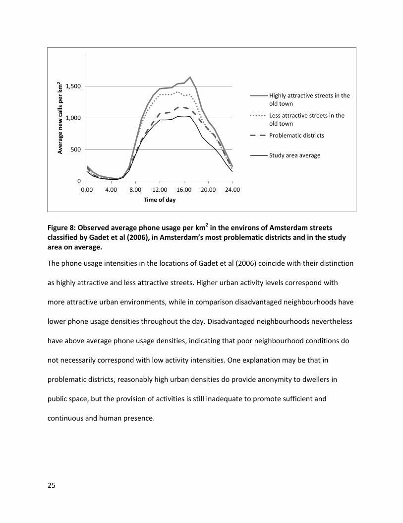
Figure 8: Observed average phone usage per km2 in the environs of Amsterdam streets classified by Gadet et al (2006), in Amsterdam’s most problematic districts and in the study area on average.
The phone usage intensities in the locations of Gadet et al (2006) coincide with their distinction
as highly attractive and less attractive streets. Higher urban activity levels correspond with
more attractive urban environments, while in comparison disadvantaged neighbourhoods have
lower phone usage densities throughout the day. Disadvantaged neighbourhoods nevertheless
have above average phone usage densities, indicating that poor neighbourhood conditions do
not necessarily correspond with low activity intensities. One explanation may be that in
problematic districts, reasonably high urban densities do provide anonymity to dwellers in
public space, but the provision of activities is still inadequate to promote sufficient and
continuous and human presence.
0
500
1,000
1,500
0.00 4.00 8.00 12.00 16.00 20.00 24.00
Ave
rage
ne
w c
alls
pe
r km
2
Time of day
Highly attractive streets in theold town
Less attractive streets in theold town
Problematic districts
Study area average

26
Figure 9: Estimated average hourly contribution per day of activities at home and other activities to phone usage in the environs of Amsterdam streets classified by Gadet et al (2006), in Amsterdam’s most problematic districts and in the study area on average. For the sake of simplicity, spatial interdependencies are ignored here.
Figure 9 shows average hourly effects of activities at home computed using inhabitant densities
and their hourly estimated effects on phone usage divided by 24 versus the similarly computed
effects of all other modelled activities. This figure clearly shows that neighbourhood
attractiveness corresponds with land-use configurations that cause higher activity intensities
and a greater degree of activity mixing. Here, in more attractive areas, there is a more equal
distribution between home-related activities and other activities. On the other side of the coin,
in Amsterdam’s most problematic districts, activities away from home contribute much less to
local activity intensities than they do on average in the study area. We conclude that
neighbourhoods that fare better coincide with urban areas that, due to their land-use
0
250
500
750
Highlyattractive inthe old town
Less attractivein the old
town
Study areaaverage
Problematicdistricts
Esti
mat
ed
ave
rage
mo
de
lled
ph
on
e u
sage
d
en
siti
es
pe
r h
ou
r p
er
wo
rkin
g d
ay
Activities at home
Other activities
27
configurations, have higher activity intensities and more equal activity mixes. This agrees with
Jacobs’s (1962) observations.
5 Conclusions and discussion
In this paper we use mobile phone usage data recorded in Amsterdam, the Netherlands, to
investigate expectations originally posed by Jacobs (1962) that dense and mixed land-use
configurations are related to higher and prolonged urban activity intensities. Our evidence
confirms that land-use densities are associated with activity levels; that different land uses are
associated with different activity dynamics; and that colocated land uses have synergetic or
multiplier effects that prolong activity levels. We additionally test Jacobs’s expectation that
neighbourhoods accommodating higher activity levels and mixed activity provisions coincide
with advantaged neighbourhoods. Our results confirm that areas that are considered attractive
have higher urban activity intensities, while in such areas the more mixed provision of activities
stands out; in contrast, activity intensities are much lower and activities at home are
overrepresented in Amsterdam’s most disadvantaged districts.
Although the evidence uncovered supports the development of dense and mixed land uses, a
number of factors need consideration before prompting such developments. First of all, the
economic value of higher and prolonged urban activity levels is difficult to estimate, and its
impact on vitality is unclear. The development of dense and mixed-use environments is
complex and costly, and real estate developers therefore prefer simpler projects (Coupland,
1997; Majoor, 2006). Thus, especially in times of weak real estate markets, dense and mixed
land-use projects are unlikely to be considered. We therefore agree with Rowley (1996) that,

28
above all, it is important that urban planners should strive to preserve those urban areas where
land-use patterns encourage high and extended activity intensities, and perhaps apply flexible
zoning schemes that allow new mixed land-use patterns to emerge.

29
References
ACA, 2004, Location Location Location: The Future Use of Location Information to Enhance the Handling of Emergency Mobile Phone Calls (Australian Communications Authority, Melbourne) Ahas R, Silm S, Järv O, Saluveer E, Tiru M, 2010, "Using mobile positioning data to model locations meaningful to users of mobile phones" Journal of Urban Technology 17(1) 3–27 Anselin L, 2001, “Spatial econometrics”, in A Companion to Theoretical Econometrics Ed. B H Baltagi (Blackwell Publishing, Malden) pp 310–330 Anselin L, Lozano-Gracia N, 2008, “Errors in variables and spatial effects in hedonic house price models of ambient air quality” Empirical Economics 34 5–34 Arbia G, 1989, Spatial Data Configuration in Statistical Analysis of Regional Economic and Related Problems (Kluwer Academic Publishers, Dordrecht) Bicknese L, Slot J, Hylkema C, 2007, Probleemwijken in Amsterdam (Municipality of Amsterdam, Amsterdam) Bonnes M, Bonaiuto M, Ercolani A P, 1991, “Crowding and residential satisfaction in the urban environment: a contextual approach” Environment and Behavior 23(5) 531–552 Breedveld K, Van den Broek A, De Haan J, Harms L, Huysmans F, Van Ingen E, 2006, De tijd als spiegel (Social and Cultural Planning Office, The Hague) Calabrese F, Colonna M, Lovisolo P, Parata D, Ratti C, 2007, Real-Time Urban Monitoring Using Cellular Phones: A Case-Study in Rome (Massachusetts Institute of Technology, Cambridge) Cervero R, 1996, "Mixed land-uses and commuting: evidence from the American Housing Survey" Transportation Research Part A: Policy and Practice 30(5) 361–377 Chan Y-K, 1999, “Density, crowding, and factors intervening in their relationship: evidence from a hyper-dense metropolis” Social Indicators Research 48 103–124 Cloïn M, Kamphuis C, Schols M, Tiessen-Raaphorst A, Verbeek D, 2011, Nederland in een dag (Social and Cultural Planning Office, The Hague) Coleman A, 1985, Utopia on Trial: Vision and Reality in Planned Housing (Shipman, London) Coupland A, 1997, "An introduction to mixed use development", in Reclaiming the City: Mixed Use Developments (E & FN Spon, London) pp 1–25

30
Currid E, Williams S, 2010, "The geography of buzz: art, culture and the social milieu in Los Angeles and New York" Journal of Economic Geography 10 423–451 De Haan J, De Hart J, Huysmans F, 2004, Trends in Time. The use and organization of Time in the Netherlands, 1975 - 2000 (Social and Cultural Planning Office, The Hague) Fischer C S, Baldassare M, Ofshe R J, 1975, “Crowding studies and urban life: a critical review” Journal of the American Institute of Planners 41(6) 406–418 Gadet J, Bobic M, Van Baaren M, Van Oosteren C, Van Zanen K, Van de Ven J, Heit R, Bosch N, 2006, Aantrekkende stadsmilieus: een planologisch-stedenbouwkundig ontwikkelingsperspectief (Municipality of Amsterdam, Amsterdam) Gans H J, 1991, People, Plans and Policies (Columbia University Press, New York) Grant J, 2002, “Mixed use in theory and practice: Canadian experience with implementing a planning principle” Journal of the American Planning Association 68(1) 71–84 Hoppenbrouwer E, Louw E, 2005, “Mixed-use development: theory and practice in Amsterdam's Eastern Docklands” European Planning Studies 13(7) 967–983 Jacobs J, 1962, The Death and Life of Great American Cities (Jonathan Cape, London) Jacobs-Crisioni C G W, Rietveld P, Koomen E, 2014, “The impact of spatial aggregation on urban development analyses” Applied Geography 47 46–56 Järv O, Ahas R, Saluveer E, Derudder B, Witlox F, 2012, “Mobile phones in a traffic flow: a geographical perspective to evening rush hour traffic analysis using call detail records” PLoS ONE 7(11) e49171 Kadaster, 2013, Base Administration of Addresses and Buildings (Kadaster, Apeldoorn) KPN, 2011, Annual Report 2010 (KPN, The Hague) LeSage J P, Fischer M M, 2008, “Spatial growth regressions: model specification, estimation and interpretation” Spatial Economic Analyses 3(3) 275–304 Majoor S J H, 2006, “Conditions for multiple land use in large-scale urban projects” Journal of Housing and the Built Environment 21 15–32 Manaugh K, Kreider T, 2013, “What is mixed use? Presenting an interaction method for measuring land use mix” Journal of Transport and Land Use 6(1) 63–72

31
Montgomery J, 1995, “Urban vitality and the culture of cities” Planning Practice and Research 10(2) 101–110 Openshaw S, 1984, The Modifiable Areal Unit Problem (Geo Books, Norwich) Petterson G, 1997, “Crime and mixed use development”, in Reclaiming the City: Mixed use Developments Ed. A Coupland (E & FN Spon, London) pp 179–198 Ratti C, Pulselli R M, Williams S, Frenchman D, 2006, “Mobile landscapes: using location data from cell phones for urban analysis” Environment and Planning B: Planning and Design 33(5) 727–748 Reades J, Calabrese F, Ratti C, 2009, “Eigenplaces: analysing cities using the space-time structure of the mobile phone network” Environment and Planning B: Planning and Design 36 824–836 Roberts M, Lloyd-Jones T, 1997, “Mixed uses and urban design”, in Reclaiming the City: Mixed Use Developments Ed. A Coupland (E & FN Spon, London) pp 149–176 Rodenburg C, Vreeker R, Nijkamp P, 2003, “Multifunctional land use: an economic perspective”, in The Economics of Multifunctional Land Use Eds P Nijkamp, C Rodenburg, R Vreeker (Shaker Publishing, Maastricht) pp 3–15 Rowley A, 1996, “Mixed-use development: ambiguous concept, simplistic analysis and wishful thinking?” Planning Practice & Research 11(1) 85–97 Silm S, Ahas R, 2010, “The seasonal variability of population in Estonian municipalities” Environment and Planning A 42(10) 2527–2546 Statistics Netherlands, 2006, Core Statistics Dutch Postcode Areas 2004 (Statistics Netherlands, Voorburg) Stead D, Hoppenbrouwer E, 2004, “Promoting an urban renaissance in England and the Netherlands” Cities 21(2) 119–136 Vreeker R, De Groot H L F, Verhoef E T, 2004, “Urban multifunctional land use: theoretical and empirical insights on economies of scale, scope and diversity” Built Environment 30(4) 289–307 Wheeler D, Tiefelsdorf M, 2005, “Multicollinearity and correlation among local regression coefficients in geographically weighted regression” Journal of Geographical Systems 7 161–187

Appendix I: Spatial distribution of explanatory variables
In Table A1 correlations between all explanatory variables are given, followed Figure A1, which
shows the spatial distribution of those variables. The correlations were weighted using the
method outlined in section 2.1 in the main article. Regarding the map series, it is important to
note that the modelled best serving cells topology cannot be disclosed. Instead, administrative
boundaries of 120 neighbourhoods in the study area have been used, to which all variables
have been spatially aggregated from their original levels. The table and map make clear that
land-use interactions have very similar spatial patterns, which may cause concerns regarding
multicollinearity issues. However, omitting interaction effect variables did not greatly affect
model results, and model results are furthermore reasonably consistent over time (see
Appendix II). This leads us to believe there are no severe multicollinearity problems in the
models presented.
Table A1: Correlation between explanatory variables
INH
BU
S
SH
MP
BU
S x
SH
BU
S x
MP
SH x
MP
TS
MET
RO
MW
AY
Inhabitant density (INH) 1.00
Business density (BUS) -0.15 1.00 Shop density (SH) -0.03 0.07 1.00
Meeting place density (MP) -0.08 0.04 0.30 1.00 Interaction BUS x SH -0.16 0.25 0.75 0.25 1.00
Interaction BUS x MP -0.16 0.31 0.41 0.73 0.59 1.00 Interaction SH x MP -0.17 0.01 0.76 0.47 0.64 0.55 1.00
Tourist square (TS) 0.00 0.05 0.27 0.25 0.31 0.36 0.32 1.00 Metro station (MS) -0.01 0.07 0.00 -0.01 -0.01 -0.02 -0.03 -0.04 1.00
Motorway (MWAY) -0.25 0.00 -0.15 -0.13 -0.11 -0.10 -0.11 -0.08 -0.08 1.00 Railway station 0.03 -0.01 -0.01 -0.04 -0.02 -0.04 -0.03 -0.02 0.14 0.03

Figure A1: Maps of explanatory variables
Appendix II: Regression results using averaged phone usage densities from different
time frames
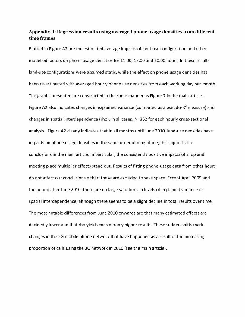
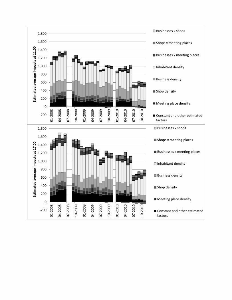
Plotted in Figure A2 are the estimated average impacts of land-use configuration and other
modelled factors on phone usage densities for 11.00, 17.00 and 20.00 hours. In these results
land-use configurations were assumed static, while the effect on phone usage densities has
been re-estimated with averaged hourly phone use densities from each working day per month.
The graphs presented are constructed in the same manner as Figure 7 in the main article.
Figure A2 also indicates changes in explained variance (computed as a pseudo-R2 measure) and
changes in spatial interdependence (rho). In all cases, N=362 for each hourly cross-sectional
analysis. Figure A2 clearly indicates that in all months until June 2010, land-use densities have
impacts on phone usage densities in the same order of magnitude; this supports the
conclusions in the main article. In particular, the consistently positive impacts of shop and
meeting place multiplier effects stand out. Results of fitting phone-usage data from other hours
do not affect our conclusions either; these are excluded to save space. Except April 2009 and
the period after June 2010, there are no large variations in levels of explained variance or
spatial interdependence, although there seems to be a slight decline in total results over time.
The most notable differences from June 2010 onwards are that many estimated effects are
decidedly lower and that rho yields considerably higher results. These sudden shifts mark
changes in the 2G mobile phone network that have happened as a result of the increasing
proportion of calls using the 3G network in 2010 (see the main article).
-200
0
200
400
600
800
1,000
1,200
1,400
1,600
1,800
01
-20
08
04
-20
08
07
-20
08
10
-20
08
01
-20
09
04
-20
09
07
-20
09
10
-20
09
01
-20
10
04
-20
10
07
-20
10
10
-20
10
Esti
mat
ed
ave
rage
imp
acts
at
11
.00
Businesses x shops
Shops x meeting places
Businesses x meeting places
Inhabitant density
Business density
Shop density
Meeting place density
Constant and other estimatedfactors
-200
0
200
400
600
800
1,000
1,200
1,400
1,600
1,800
01
-20
08
04
-20
08
07
-20
08
10
-20
08
01
-20
09
04
-20
09
07
-20
09
10
-20
09
01
-20
10
04
-20
10
07
-20
10
10
-20
10
Esti
mat
ed
ave
rage
imp
acts
at
17
.00
Businesses x shops
Shops x meeting places
Businesses x meeting places
Inhabitant density
Business density
Shop density
Meeting place density
Constant and other estimatedfactors

Figure A2: Results from fitting this paper’s model on phone-usage data for separate monthly averages: estimated impacts of land-use densities on phone usage at different hours (first three graphs), levels of rho and pseudo-R2 (last graph)
-200
0
200
400
600
800
1,000
1,200
1,400
1,600
1,800
01
-20
08
04
-20
08
07
-20
08
10
-20
08
01
-20
09
04
-20
09
07
-20
09
10
-20
09
01
-20
10
04
-20
10
07
-20
10
10
-20
10
Esti
mat
ed
ave
rage
imp
acts
at
20
.00
Businesses x shops
Shops x meeting places
Businesses x meeting places
Inhabitant density
Business density
Shop density
Meeting place density
Constant and other estimatedfactors
0.00
0.25
0.50
0.75
1.00
01/2008 06/2008 12/2008 06/2009 12/2009 06/2010 12/2010
Rho 20.00
Rho 17.00
Rho 11.00
Pseudo-R² 20.00
Pseudo-R² 17.00
Pseudo-R² 11.00

Appendix III: Streets considered very or less attractive and problematic districts
Table A2: classification of attractiveness of streets in Amsterdam, categorised according to data from Gadet et al (2006).
Streets considered attractive Streets considered less attractive
Beethovenstraat Admiraal de Ruyterweg Eerste van der Helststraat Johannes Verhulststraat Frans Halsstraat Kinkerstraat Haarlemmerdijk Lelylaan Hoogte Kadijk Oostelijke Handelskade
Prinsengracht Postjesweg Utrechtsestraat Spaarndammerstraat
Tweede van der Helststraat
Van der Pekstraat
Zuidplein
Table A3: neighbourhood list compiled by the Dutch Ministry for Housing, Neighbourhoods and Integration and published by Bicknese et al (2007).
Problematic neighbourhoods in Amsterdam 4-digit postcode
Nieuwendam Noord 1024 Volewijck 1031, 1032
Landlust 1055 Van Galenbuurt 1056 De Krommert 1057 Kolenkitbuurt 1061 Westlandgracht 1062 Slotermeer Noord-oost & Zuid-west 1063, 1064
Slotervaart 1065 Geuzenveld 1067 Osdorp Oost 1068 Osdorp Midden 1069 Transvaalbuurt 1092
Indische buurt West 1094 Bijlmer Oost 1103, 1104