university of alberta · abstract the phase behavior and thermophysical properties of heavy...
TRANSCRIPT

University of Alberta
Phase Behavior and Thermophysical Properties of Athabasca Bitumen
and Athabasca Bitumen + Toluene Mixtures in Near-critical Water
by
Mohammad Javad Amani
A thesis submitted to the Faculty of Graduate Studies and Research
in partial fulfillment of the requirements for the degree of
Doctor of Philosophy
in
Chemical Engineering
Department of Chemical and Materials Engineering
©Mohammad Javad Amani
Spring 2014
Edmonton, Alberta
Permission is hereby granted to the University of Alberta Libraries to reproduce single copies of this thesis and to lend or sell such copies for private, scholarly or scientific research purposes only. Where the thesis is
converted to, or otherwise made available in digital form, the University of Alberta will advise potential users of the thesis of these terms.
The author reserves all other publication and other rights in association with the copyright in the thesis and ,
except as herein before provided, neither the thesis nor any substantial portion thereof may be printed or otherwise reproduced in any material form whatsoever without the author's prior written permission.

Abstract
The phase behavior and thermophysical properties of heavy hydrocarbons + water
at elevated temperatures underpins development and implementation of
coordinated production and refining processes, where for example, bitumen is
produced by a SAGD method (steam assisted gravity drainage) and the resulting
bitumen + water mixtures are then upgraded directly. Supercritical water is an
effective solvent for hydrocarbons at high temperatures and reduces coke
formation when present during upgrading. In this work, the thermophysical
properties and phase behavior of Athabasca bitumen + solvent + water mixtures
are investigated and the results are compared to large molecule size hydrocarbons
+ water binaries available in the literature. Experiments were conducted using a
variable-volume X-ray view cell in the broad range of temperature and pressure
up to 644 K and 26.2 MPa near the critical point of water. The P-x and PT phase
diagrams for pseudo-binaries and pseudo-ternaries of bitumen + solvent + water
are constructed and single phase bitumen-rich regions are identified. The
solubility of water in the hydrocarbon-rich phase, a key parameter in the design of
water-based upgrading reactors, is evaluated to provide a reliable reference for
solubility of water in high-molar-mass hydrocarbons. The accuracy of water
solubility in the hydrocarbon-rich phase and phase behavior boundaries were
validated by reproducing pressure-composition diagrams at fixed temperature and
pressure-temperature diagrams for 1-methylnaphthalene + water and toluene +
water binaries presented in the literature. Impacts of toluene addition on solubility
of water in Athabasca bitumen + water mixtures are described. Furthermore, the

density of bitumen phase and the impact of water solubility on the volume of
mixing for the bitumen-rich liquid phase are discussed. A simple and robust
model is developed to predict solubility of water in ill-defined hydrocarbons
below their upper critical end point. An empirical model is also proposed to
extend the solubility data to higher temperatures (> 673 K) where the mixtures are
reactive. This body of work including phase diagrams, solubility and density data
and models are expected to provide essential data to define promising regimes of
temperature, pressure and composition for the application of water in hydrocarbon
resource processing.

Acknowledgments
I express my sincere gratitude and appreciation to my advisors, Professor John M. Shaw
for providing me with the great opportunity to work in the research area of petroleum
thermodynamics, for his deep knowledge, expert guidance, mentorship, huge
encouragement and support at all levels.
I thank Professor Murray R. Gray, my co-supervisor, for offering valuable and
constructive comments. His unique feedback and suggestion on my research are highly
appreciated.
In addition, I am very grateful to Professor Marco Satyro, for his worthy help and patient
guidance during my project. I can’t say thank you enough to him for his enthusiasm and
encouragement.
I thank Professor Arno de Klerk for his helpful discussions and comments.
I take this opportunity to express my gratitude to all of my colleagues in petroleum
thermodynamics research group who have been instrumental in the successful completion
of this project. I particularly appreciate Keivan Khaleghi for his kind guidance to
understand the basics and operation of the X-ray view cell. I am grateful to Mildred
Becerra, the lab manager of Petroleum Thermodynamic Research Lab, for providing a
safe working environment, assistance and technical support, especially during the two
laboratory moves we endured, and equipment, and samples as needed. I appreciate Slava
Fedossenko for his help in laboratory move.
I also thank ; Office Support, Computer Support, Machine Shop, and Instrument Shop
staff in the Chemical and Materials Engineering Department at U of A for their help and
assistance.
My gratitude goes to my friends; Ali A., Ali Sh., Amin, Ata, Ehsan, Farzad, Hesam,
Kasra, Keivan Kh., Keivan N., Milad, Mohtada, Mojtaba, Nafiseh, Nasseh, Nima,
Parastoo, Reza, Robert, Roohi, Roya, Sajjad, Saman, Somayeh and all other beloved
friends who helped me and create many wonderful times in Edmonton.
My sincere appreciation goes to my mother and father for their unconditional love, care
and support. I will never truly be able to express my deepest appreciation to both of you. I
love you and owe all my success in life to you forever.

Funding provided by the Centre for Oil Sands Innovation (COSI) and the sponsors of the
NSERC Industrial Research Chair in Petroleum Thermodynamics (Natural Sciences and
Engineering Research Council of Canada (NSERC), Alberta Innovates Energy and
Environment Solutions, British Petroleum, ConocoPhillips Canada, Halliburton Energy
Services, KBR Energy and Chemical, Imperial Oil Resources, Nexen Inc., Shell Canada
Ltd., Total E&P Canada Ltd., Virtual Materials Group) is gratefully acknowledged.

Contents
CHAPTER 1. INTRODUCTION ........................................................................................ 1
1.1 BACKGROUND AND THESIS OUTLINE ..................................................................................................1
1.2 MOTIVATION OF THE RESEARCH .......................................................................................................3
1.2.1 Surface bitumen upgrading............................................................................................3
1.2.2 In-situ bitumen combination SAGD................................................................................4
1.3 REVIEW ON OTHER PROCESSES INCLUDING HYDROCARBONS AND WATER AT HIGH TEMPERATURES .............5
1.3.1 Supercritical extraction of oil shale and heavy fractions .............................................5
1.3.2 Contaminated soils remediation ....................................................................................6
1.3.3 Oxidation and thermal reaction of hydrocarbons in water .........................................6
1.4 REVIEW ON THERMOPHYSICAL PROPERTIES AND PHASE BEHAVIOR OF HYDROCARBON + WATER MIXTURES
7
1.4.1 Phase behavior basics.....................................................................................................7
1.4.2 Phase equilibria of water + hydrocarbon mixtures.......................................................9
1.4.2.1 Water + n-Alkanes binary mixture data at high pressure and temperature .............. 10
1.4.2.2 Water + aromatics binary mixtures at elevated temperatures and pressures ........... 11
1.4.2.3 Water + heavy oil and multi-component hydrocarbon mixtures .............................. 11
1.4.3 Solubility of water in hydrocarbons ............................................................................ 12
1.4.4 Volumetric behavior of hydrocarbons + water mixtures........................................... 15
1.4.5 Water + hydrocarbons phase behavior modeling...................................................... 15
1.4.5.1 Application of cubic equations of state to calculate water + hydrocarbon phase
equilibria 16
1.4.5.2 Advanced non-cubic equations of state .................................................................. 17
1.4.5.3 Empirical and semi-empirical approach .................................................................. 19
1.5 OBJECTIVES ................................................................................................................................ 20
1.6 OVERVIEW OF THE RESEARCH METHODOLOGY................................................................................. 21
1.7 REFERENCES ............................................................................................................................... 25
CHAPTER 2. PHASE BEHAVIOR OF ATHABASCA BITUMEN + WATER MIXTURES AT HIGH
TEMPERATURE AND PRESSURE ..................................................................................... 34
2.1 INTRODUCTION ........................................................................................................................... 34
2.2 MATERIALS AND METHODS ........................................................................................................... 36
2.2.1 Experimental apparatus .............................................................................................. 36
2.2.2 Experimental method validation measurements....................................................... 39
2.2.2.1 1-Methylnaphthalene + water mixtures .................................................................. 39
2.2.2.2 Toluene + water mixtures....................................................................................... 42

2.2.3 Phase diagram construction ....................................................................................... 45
2.3 RESULTS AND DISCUSSION ............................................................................................................ 46
2.4 CONCLUSION .............................................................................................................................. 58
2.5 REFERENCES ............................................................................................................................... 59
CHAPTER 3. VOLUME OF MIXING AND SOLUBILITY OF WATER IN ATHABASCA BITUMEN AT
HIGH TEMPERATURE AND PRESSURE ............................................................................. 63
3.1 INTRODUCTION ........................................................................................................................... 63
3.2 EXPERIMENTS AND METHODOLOGY ............................................................................................... 66
3.2.1 Water solubility measurement validation .................................................................. 67
3.2.2 Liquid density measurement validation ..................................................................... 69
3.3 RESULTS AND DISCUSSION ............................................................................................................ 71
3.3.1 Solubility of water in bitumen ..................................................................................... 71
3.3.2 Excess volume of the Athabasca bitumen-rich liquid phase ..................................... 79
3.4 CONCLUSION .............................................................................................................................. 84
3.5 REFERENCES ............................................................................................................................... 84
CHAPTER 4. THE PHASE BEHAVIOR OF ATHABASCA BITUMEN + TOLUENE + WATER TERNARY
MIXTURES 91
4.1 INTRODUCTION ........................................................................................................................... 91
4.1.1 Solubility of water in hydrocarbons ............................................................................ 92
4.1.2 Phase behavior of hydrocarbon + water mixtures..................................................... 93
4.2 EXPERIMENTAL SET-UP AND METHODOLOGY ................................................................................... 93
4.3 RESULTS AND DISCUSSION ............................................................................................................ 95
4.3.1 Phase Diagrams for Bitumen + Toluene + Water Mixtures....................................... 95
4.3.2 Water solubility in bitumen + toluene mixtures at high temperatures .................. 103
4.3.3 Density of water-rich and hydrocarbon-rich liquid phases ..................................... 105
4.3.4 Density differences between the water-rich and hydrocarbon-rich liquid phases 108
4.3.5 Phase behavior type transition ................................................................................. 110
4.4 CONCLUSIONS .......................................................................................................................... 114
4.5 REFERENCES ............................................................................................................................. 114
CHAPTER 5. CORRELATIONS FOR CALCULATING THE SOLUBILITY OF WATER IN ILL-DEFINED
HYDROCARBONS .......................................................................................................118
5.1 INTRODUCTION ......................................................................................................................... 118
5.2 MODEL DEVELOPMENT .............................................................................................................. 121

5.2.1 Model A: solubility of water in hydrocarbons below the UCEP of hydrocarbon +
water mixtures .......................................................................................................................... 121
5.2.2 Model B: solubility of water in hydrocarbon-rich liquids above the UCEP of
hydrocarbon + water mixtures................................................................................................. 125
5.3 RESULTS AND DISCUSSION .......................................................................................................... 131
5.3.1 Model A ...................................................................................................................... 131
5.3.1.1 Model A Fitting Results......................................................................................... 131
5.3.1.2 Model A Testing and Evaluation............................................................................ 133
5.3.1.3 Impact of input parameter uncertainty on predicted water solubility outcomes. .... 141
5.3.2 Model B – Water Solubility in hydrocarbons above the UCEP ................................ 143
5.4 CONCLUSION ............................................................................................................................ 146
5.5 REFERENCES ............................................................................................................................. 146
CHAPTER 6. CONCLUSIONS AND REMARKS .................................................................151
6.1 FUTURE WORKS AND RECO MMENDATIONS.................................................................................... 154
APPENDIX 1. STANDARD OPERATING PROCEDURES OF THE X-RAY VIEW CELL .....................155
APPENDIX 2. SUPPLEMENTARY DATA ...........................................................................174
APPENDIX 3. IMAGE PROCESSING CODE IN MATLAB .......................................................190

List of Tables
Table 1.1. Available literature data for solubility of water in pure hydrocarbons above 373.2 K... 13
Table 1.2. Solubility of water in reservoir fluids and petroleum fractions. ....................................... 15
Table 2.1. Properties for Athabasca bitumen [21].............................................................................. 37
Table 2.2. Experimental phase behavior data for 1-methylnaphthalene + water mixtures at 573 K.
................................................................................................................................................................ 41
Table 2.3. Observed L=V critical points for toluene + water binary mixtures. .................................. 43
Table 2.4. LLV three-phase pressure for toluene + water mixtures. .................................................. 44
Table 2.5. LLV/LL and L2V/L phase boundaries for Athabasca bitumen + water mixtures .............. 54
Table 3.1. Water solubility in toluene (wt %) ...................................................................................... 69
Table 3.2. Water solubility in 1-methylnaphthalene (wt %) .............................................................. 69
Table 3.3. Saturated density of liquid 1-methylnaphthalene (kg/m3) ............................................... 71
Table 3.4. Solubility of water in the bitumen-rich liquid phase. ........................................................ 78
Table 3.5. Density of Athabasca bitumen ........................................................................................... 78
Table 3.6. Bitumen-rich phase density and excess specific volume data .......................................... 83
Table 4.1. LLV/LL and L2V/L2 boundaries of {(1-w) bitumen + (w) toluene} + water mixtures at a
weight fraction of w=0.443. ............................................................................................................... 100
Table 4.2. LLV/LL and L2V/L2 boundaries of {(1-w) bitumen + (w) toluene} + water mixtures at a
weight fraction of w=0.668. ............................................................................................................... 102
Table 4.3. Solubility of water in {(1-w) bitumen + (w) toluene} blends at w=0.443 and 0.668.
Water solubility is reported in weight fraction. ................................................................................ 104
Table 4.4. Density of water-saturated toluene .................................................................................. 107
Table 4.5. Density of water-saturated 1-methylnaphthalene vs. predicted ideal mixing density. . 107
Table 4.6. Density of (1-w) bitumen + (w) toluene at w=0.667 weight fraction. ........................... 112
Table 4.7. Density of water saturated bitumen-rich phase for {(1-w) bitumen + (w) toluene} +
water mixtures at w=0.448 and 0.667............................................................................................... 113
Table 5.1. List of substances and their properties used fit parameters for Model A (equation 5-4)
.............................................................................................................................................................. 128
Table 5.2. Parameters for Model A (equation 5-4)........................................................................... 130
Table 5.3. Overview of Model A performance .................................................................................. 130
Table 5.4. Properties of heavy oils used to test Model A, and to obtain coefficients for Model B 143

Table 5.5. Solubility of water in Athabasca bitumen Chapter 3 [35] and experimentally derived K
values. .................................................................................................................................................. 145

List of Figures
Figure 1.1. Operating conditions for some current bitumen production and upgrading processes. .5
Figure 1.2. Characteristics of binary phase behavior by Type according to the van Konynenburg
and Scott classification scheme. .............................................................................................................9
Figure 1.3. Types II and III (a and b) binary phase behavior projections. Pure component vapor
pressure curves are shown on pressure–temperature (P–T) diagrams by dashed lines, solid lines
represent both liquid–gas (LV) and liquid–liquid (LL) critical curves and three-phase lines (LLV
lines) are represented by dotted-dashed. Dark circles and open circles stand for pure component
critical points and upper critical end points (UCEP) respectively [29]. .............................................. 10
Figure 1.4. An illustration for X-ray transmission image. .................................................................. 22
Figure 1.5. Athabasca bitumen + 49.9% water at 573 K and 8.8 MPa ............................................. 23
Figure 2.1. Schematic pressure-temperature projections for Type II, IIIa and IIIb phase behavior.
Pure component vapor pressure curves ( ), liquid-gas (LV) and liquid-liquid (LL) critical loci ( ),
liquid-liquid vapor lines ( ), pure component critical points ( ) and critical end points ( ).......... 35
Figure 2.2. X-ray view cell apparatus schematic ................................................................................ 38
Figure 2.3. Vapor phase volume trends adjacent to LV/L and LLV/LL boundaries for 1-
methylnaphthalene + water mixtures at 573 K. Data: LLV/LL: 78.9 wt % 1-methylnaphthalene ( ),
LV/L: 78.3 wt % 1-methylnaphthalene ( ) and LV/L: 96.3 wt % 1-methylnaphthalene ( ). Linear
extrapolation of experimental volume data ( ). Trends computed using the Peng-Robinson
equation of state [35] with Kij =0.26 ( ). ........................................................................................ 40
Figure 2.4. Pressure-composition diagram for the 1- methylnaphthalene + water binary at 573 K.
Phase behavior boundaries identified by Christensen [17] ( ). Phase behavior and phase behavior
boundaries identified in this work: LV data ( ), LV/L boundary values ( ), and LLV/LL boundary
value ( ). ................................................................................................................................................ 41
Figure 2.5. Typical x-ray images for the toluene (88.4 wt %) + water binary. The vapor phase (V)
has a low intensity. The toluene-rich liquid (L1) has an intermediate intensity (light liquid) and the
water rich liquid (L2) has a low intensity (dense liquid) . The magnetic stirrer (black sphere at the
base of the cell) and the bellows (black cylinder at the top of the cell) are visible in some of the
images. L1/ L2 ( ) and L1/V ( ) interfaces are shown in the images where present................ 43
Figure 2.6. Pressure-temperature projection for the toluene + water binary (Type IIIa). The solid
curves ( ) are the water and toluene vapor pressures [27]. The solid triangles, Brunner [19], ( )
and the open diamonds, this work, ( ) are points on the L=V critical locus. Solid squares, Brunner

[19], ( ), crosses, Anderson [28], (×), open triangles, Chandler [29], ( ) and stars, this work, ( )
are LLV three-phase points................................................................................................................... 45
Figure 2.7. Typical x-ray images for Athabasca bitumen (AB) + water mixtures at 613.5 K.
liquid/liquid( ) and liquid/vapor ( ) interfaces are shown in the images where present...... 46
Figure 2.8. Pressure-temperature diagrams for Athabasca bitumen + water mixtures at fixed
Athabasca bitumen wt %: a) 9.2 wt %, b) 55.9 wt %, c) 66.3 wt %, d) 73.3 wt %, e) 78.3 wt %, f)
87.7 wt % wt %, g) 88.7 wt %, h) 96.6 wt %. The water vapor pressure curve is shown in each
figure as a dotted curve ( ) terminating at a critical point designated with a solid circle ( ).
Liquid-vapor and liquid-liquid-vapor equilibrium data, are shown as open circles ( ) and open
triangles ( ) respectively. Points on LV/L and LLV/LL boundaries are shown as solid squares ( ) and
( ), and solid curves ( ) trace the LLV/LL and LV/L boundaries. Boundaries designated with a
dash-dot lines ( ) are illustrative and were not identified experimentally.................................... 51
Figure 2.9. Pressure-composition diagrams for Athabasca bitumen + water at fixed temperature:
a) 583.2 K, b) 623.2 K, c) 644 K. Measured liquid-vapor ( ) and liquid-liquid-vapor ( ) equilibrium
data are shown. The vapor pressure of water obtained from [27]. Solid lines ( ) show the LL/LLV
and L2V/ L2 boundaries where points on these boundaries are designated with ( ) and ( ),
respectively, and the L2V/LLV boundary defined by the vapor pressure of water ( ). Boundaries
designated with a dash-dot lines ( ) are illustrative and were not identified experimentally..... 53
Figure 2.10. Schematic pressure-temperature projection and pressure-composition at fixed
temperature phase diagrams for the Athabasca bitumen + water pseudo binary mixture. Pure
component vapor pressure curves ( ), liquid-gas (L=V) and liquid-liquid (L=L) critical loci ( ),
liquid-liquid vapor curve ( ), L=V and L=L critical points ( ) and K-point ( ). ................................ 57
Figure 2.11. Thermal reaction rates for 9.2 ( ) and 66.3 ( ) wt % Athabasca bitumen + water
mixtures. ................................................................................................................................................ 58
Figure 3.1. Type IIIb pressure-temperature projection for water + hydrocarbon binary mixtures. (
) critical points for the water and the hydrocarbon, and ( ) the UCEP for the mixture. ( ) and (
) are the critical locus and LLV three-phase curve respectively and ( ) denotes vapor/bubble
pressure curves (Chapter 2).................................................................................................................. 65
Figure 3.2. The X-ray view cell schematic. The view-cell is equipped with a variable volume
bellows and a magnetic stirrer. ........................................................................................................... 67
Figure 3.3. P-x diagrams for tetralin + water at 573.2 K: (a) mass-based and (b) mole-based. The
experimental data ( ) and the three-phase line ( ) are from Christensen [37] and ( ) is the
estimated composition of the saturated tetralin-rich liquid. ............................................................. 68

Figure 3.4. The solubility of water in: a) toluene (this work ( ), Anderson et al. [32] ( ), Brown et
al. [24] ( ), Chandler et al. [31] ( ), Jou et al. [65] ( ) and Neely et al. [34] (+)) and in b) 1-
methylnaphthalene (this work ( ), Economou et al. [26] ( ), Christensen et al. [37] ( ), and
compilation of the former data by Shaw et al. [21] ( )). .................................................................... 70
Figure 3.5. Pressure-composition diagrams for Athabasca bitumen + water at fixed temperature:
(a) 523.0 K (b) 548.2 K, (c) 573.1 K, (d) 583.2 K, (e) 593.1 K, (f) 603.5 K, (g) 613.4 K, (h) 623.2 K, (i)
633.8 K, (j) 644. Measured liquid-vapor ( ) and liquid-liquid-vapor ( ) equilibrium data are shown.
The vapor pressure of water obtained from [59]. Solid lines ( ) show the LL/LLV and L2V/L2
boundaries where points on these boundaries are designated with ( ) and ( ), respectively, and
the L2V/LLV boundary defined by the vapor pressure of water ( ). Boundaries designated with a
dash-dot lines ( ) are illustrative and were not identified experimentally.................................... 76
Figure 3.6. Solubility of water in Athabasca bitumen, this work ( ), and in other hydrocarbons: a)
all available hydrocarbons:, b) high molar mass compounds and heavy oils, and equation 3 -1 ( )
. Symbols: toluene ( ) [24, 31, 32], ethylbenzene ( ) [27], m-xylene (+) [32], ethylcyclohexane (-)
[27], n-octane ( ) [27], tetralin ( ) [26], 1,2,3,4-Tetrahydroquinoline [33], thianaphthene ( ) [33],
cis-decalin ( ) [26], 1-butylcyclohexane ( )[26], decane ( )[26], 1-methylnaphthalene ( ) [26], 1-
ethylnaphthalene ( ) [26], 1,4-diisopropylbenzene ( ) [26], 9,l0-dihydrophenanthrene ( ) [33],
naphtha ( , Mw = 147) [60], kerosene(×,Mw = 173) [60], lubricating oil ( , Mw = 425) [60], gross
oil mixtures ( , Mw = 425) [63], Coalinga crude oil (|, Mw = 439) [61],Huntington Beach crude oil
( , Mw = 442) [61],Peace River crude oil ( , Mw = 571) [61] Cat Canyon crude oil ( , Mw = 627)
[61] . ....................................................................................................................................................... 77
Figure 3.7. A typical volume of mixing for heavy hydrocarbon + water at temperatures lower than
the upper critical end point. ................................................................................................................. 80
Figure 3.8. Excess volume ( ) for the Athabasca bitumen-rich phase at saturation. The line
segments, (------) represent the excess volumes of unsaturated Athabasca bitumen. Temperature
is a parameter. ...................................................................................................................................... 81
Figure 3.9. The derivative of excess volume with water mass fraction obtained by analyzing excess
volume data for benzene ( ) [46, 47], toluene ( ) [46, 49], ethylbenzene ( ) [46, 49], n-hexane ( )
[50], n-decane ( ) [50], and for Athabasca bitumen ( ) this work. .................................................... 82
Figure 4.1. P-x diagrams of {(1-w) bitumen +(w) toluene} + water mixture for w=0.443 wt fraction
at 493.1 (a), 513.1 (b), 533.1 (c), 553.1 (d), 573.2 K (e). Measured liquid-vapor ( ) and liquid-
liquid-vapor ( ) equilibrium data are shown. The vapor pressure of water ( ) obtained from [32].
Solid lines ( ) show the LLV/LL and L2V/L2 boundaries where points on these boundaries are
designated with ( ) and ( ), respectively, and the LLV/L2V boundary defined by the vapor pressure

of water ( ). Boundaries designated with a dash-dot lines ( ) are illustrative and were not
identified experimentally. Bubble pressure of Athabasca bitumen + 0.448 toluene ( ) is also
shown..................................................................................................................................................... 97
Figure 4.2. P-x diagrams of {(1-w) bitumen +(w) toluene} + water mixture for w=0.668 wt fraction
at 492.7 (a), 512.8 (b), 532.6 (c), 553.2 (d), 563.2 (e), 573.3 K (f). Measured liquid-vapor ( ) and
liquid-liquid-vapor ( ) equilibrium data are shown. The vapor pressure of water ( ) obtained from
[32]. Solid lines ( ) show the LLV/LL and L2V/L2 boundaries where points on these boundaries
are designated with ( ) and ( ), respectively, and the LLV/L2V boundary defined by the vapor
pressure of water ( ). Boundaries designated with a dash-dot lines ( ) are illustrative and
were not identified experimentally. Bubble pressure of Athabasca bitumen + 0.667 toluene ( ) is
also shown. ............................................................................................................................................ 99
Figure 4.3. Solubility of water in {(1-w) bitumen +(w) toluene} mixtures for w = 0.0 i.e.: Athabasca
bitumen ( ) Chapter 3, w=0.443 ( ) and 0.668 ( ), this work, and w = 1.0 i.e.: toluene ( ) [14, 16-
19]. Computed weight fraction averaged water solubilities in bitumen + toluene mixtures based
on smoothed data: w=0.443 ( ) and 0.668 ( ) weight fraction (equation 4-4). ...................... 104
Figure 4.4. Experimental density of water-saturated toluene at the LLV/LL boundary pressure ( ).
The predicted density of the toluene-rich phase at the LL/LLV boundary pressure is based on water
and toluene densities at the LLV/LL boundary pressure, and ideal mixing (equation 4-5) ( ) using
smoothed water solubility experimental data [20]. ......................................................................... 106
Figure 4.5. Experimental density of water saturated 1-methylnaphthalene at the LLV/LL boundary
pressure ( ). The predicted density of the 1-methylnaphthalene-rich liquid phase is based water
density at the LLV/LL boundary pressure and 1 methylnaphthalene at its vapor pressure and ideal
mixing equation 4-5 ( ) using smoothed water solubility experimental data [21]..................... 106
Figure 4.6. Computed density of saturated {(1-w) bitumen + (w) toluene} mixtures at: w= 0.170
( ), 0.448 ( ), and 0.667 ( ) weight fraction toluene at the LLV/LL boundary pressure
(equation 4-5). Densities for Athabasca bitumen ( ) Chapter 3, and water ( ) [32] are shown for
completeness. Experimental data for water saturated bitumen + toluene phase at w= 0.448 ( )
and 0.667 ( ) are also shown. ............................................................................................................ 109
Figure 4.7. Approximate density inversion boundary for {(1-w) bitumen +(w) toluene} + water (
) mixtures at the LLV/LL boundary pressure. .................................................................................... 109
Figure 4.8. Experimental density of (1-w) Athabasca bitumen + (w) toluene at w= 0.667 vs
temperature ( ). The predicted density of toluene + bitumen mixtures at the saturation pressure
based on ideal mixing ( ). ............................................................................................................... 110

Figure 4.9. Schematic showing the transition from Type IIIa to Type IIIb phase behavior as the
composition of bitumen in the bitumen + toluene + water mixtures increases, from Figure (a) to
(c). The LLV curve ( ), LV and LL critical locus ( ), the saturation curve of water and
hydrocarbons ( ) are shown. The upper critical end point of the mixture is represented by ( ),
while the critical point of water and hydrocarbons are represented by ( ). .................................. 112
Figure 5.1. Solubility of water in pure hydrocarbons and reservoir fluids at temperatures above
373 K. Solubility of water in Athabasca bitumen ( ) Chapter 3 [35], Athabasca bitumen + 0.443
toluene( ) Chapter 4 [50], Athabasca bitumen + 0.668 toluene ( ) Chapter 4 [50], toluene ( ) [5,
33, 34], ethylbenzene ( ) [6], m-xylene (+) [6], ethylcyclohexane (-) [7], tetralin ( ) [9],
thianaphthene ( ) [52], cis-decalin ( ) [9], 1-butylcyclohexane ( ) [9], decane ( ) [9], 1-
methylnaphthalene ( ) [10], 1-ethylnaphthalene ( ) [10], 1,4-diisopropylbenzene ( )[10], 9,10-
dihydrophenanthrene ( ) [52], naphtha ( , Mw = 147) [47], kerosene(×,Mw = 173) [47],
lubricating oil ( , Mw = 425) [47], gross oil mixtures ( , Mw = 425) [46], Coalinga crude oil (|, Mw =
439) [48], Huntington Beach crude oil ( , Mw = 442) [48], Peace River crude oil ( , Mw = 571) [48]
and Cat Canyon crude oil ( , Mw = 627) [48].................................................................................... 122
Figure 5.2. Solubility of water in paraffins ( ), olefins ( ) and naphthenes ( ) at 293.2 ± 1 K as a
function of normal boiling point [1-12]. ............................................................................................ 123
Figure 5.3. Solubility of water in aromatic hydrocarbons a) as a function of boiling temperature at
293.2 ± 1 K ( ) and 373.2 ( ) and 477.6 ( ); b) as a function of hydrogen weight fraction 293.2 ± 1
K ( ) and 373.2 ( ) and 473.2 ( ) [1-12]. ............................................................................................ 125
Figure 5.4. P-x diagrams of Athabasca bitumen + water (a) 623.2 K and (b) 644 K. Measured
liquid-vapor ( ) and liquid-liquid-vapor ( ) equilibrium data are shown. The vapor pressure of
water obtained from [39]. Solid lines ( ) show the LL/LLV and L2V/L2 boundaries where points on
these boundaries are designated with ( ) and ( ), respectively, and the L2V/LLV boundary defined
by the vapor pressure of water ( ). Boundaries designated with a dash-dot lines ( ) are
illustrative and were not identified experimentally (Chapter 3)...................................................... 127
Figure 5.5. Calculated solubility of water in cyclohexane equation 5-4 ( ), experimental data
[40] ( ) and tentative experimental data [3] ( ). .............................................................................. 132
Figure 5.6. Error dispersion between calculated values for the solubility of water in pure
hydrocarbons and Athabasca bitumen Model A (equation 5-4) and experimental data (Table 5.1).
The ±30% deviations ( ) are also shown........................................................................................ 133
Figure 5.7. Calculated solubility of water in Athabasca bitumen ( ) using: Model A (training set),
( ) low temperature solubility model (test set) [28] , ( ) API recommended model (test set)
[32] and experimental data ( ) Chapter 3 [35] . ............................................................................... 133

Figure 5.8. Calculated solubility of water in: (a) gasoline G10 - molecular weight 82 g/mole and an
average boiling point 58.9 oC ( ) [41, 42], (b) kerosene ( ) and paraffinic oil ( ) [43]. The predicted
values using Model A ( ) and a low-temperature NRTL based solubility model ( ) [28] are
shown................................................................................................................................................... 135
Figure 5.9. Solubility of water in hydrocarbons predicted by Model A ( ) and ( ) low
temperature solubility model (kerosene) [28] compared to experimental data: (a) naphtha ( )
[47], (b) kerosene ( ) [47], (c) lubricating oil ( ) [47] and (d) fuel mixtures ( ) [46]. ...................... 137
Figure 5.10. Predicted solubility of water in oils using Model A ( ), fitted NRTL based solubility
model ( ) [28], and the corresponding experimental data [48]: (a) Coalinga ( ), (b) Huntington
Beach ( ), (c) Peace River ( ) and (d) Cat Canyon crude( ). ............................................................. 139
Figure 5.11. Predicted solubility of water in ((1-w) Athabasca bitumen + (w) toluene) + water.
Model A: w = 0.668 ( ) and 0.443 ( ); NRTL based approach: w = 0. 668 ( ) and 0.443 ( )
[28, 51]. Experimental data in Chapter 4 w = 0.668 ( ) and 0.443 ( ). ........................................... 140
Figure 5.12. 10% variation in inputs (a) average normal boiling point and (b) hydrogen weight
fraction. Predicted solubility of water in ((1-w) Athabasca bitumen + (w) toluene) + water: w =
0.668 ( ) and 0.443 ( ) Model A, and experimental data in Chapter 4 w = 0.668 ( ) and 0.443
( ). ........................................................................................................................................................ 142
Figure 5.13. Estimating K for Athabasca bitumen ( ) (evaluated based on equation 5-7 and 5-8)
using Model A (equation 5-4) + the NIST water vapor pressure equation ( ) and the LLV/LL
phase boundary pressure ( ), and Model B, equation 5-11 ( ). ............................................... 145

List of Abbreviations and Symbols
Symbol Unit Description
1-MN 1-Methylnaphthalene
AB Athabasca bitumen
H MPa/mole fraction Henry’s constant
Hwt wt fraction Elemental Hydrogen content
K MPa/wt fraction Semi-Henry’s constant
L Liquid phase
L1 Less dense liquid
L2 More dense liquid
L2V More dense liquid-vapor
L2V/L Boundary which separates liquid-vapor and liquid regions
LL Liquid-liquid
LLV Liquid- Liquid –Vapor
LLV/LV Boundary which separates LLV and LV regions
LV Liquid- Vapor
P MPa Pressure
PAHs Polycyclic Aromatic Hydrocarbons
PT Pressure-Temperature
P-x Pressure-Composition
RTD Resistance Temperature Detector
S wt fraction Solubility
T K Temperature
Tb oC Average normal boiling point
V Vapor
w wt fraction Weight fraction composition
X mole fraction Mole fraction composition

1
Chapter 1. Introduction
1.1 Background and thesis outline
Water as a solvent plays a significant role in many industrial processes. Beside the
normal properties of water at low temperatures, water presents different and interesting
properties in its critical region. The properties of near-critical and supercritical water are
used in the design and operation of processes worldwide. Oil extraction,
secondary/tertiary oil recovery methods, supercritical extraction, oxidative reactions,
municipal and industrial wastes destruction, hydrothermal synthesis and hydrolysis
reactions are important instances that involve hydrocarbon + water mixtures at elevated
temperatures. One of the possible applications of high temperature water is in heavy
oil/bitumen extraction and upgrading. The use of water in bitumen production and
upgrading processes may provide a significant advantage over current practice due to the
possible elimination of asphaltene precipitation effects.
Asphaltenes, comprising up to 30 wt % of vacuum residues, pose serious problems in oil
production, transport and upgrading processes. A detailed understanding of their structure
and behavior are essential to control/avoid possible problems particularly in heavy oil and
bitumen production and refining processes. Many questions about the nature of
bitumen/asphaltene behavior and their characteristics are still unanswered and the
economic impact of this uncertainty is significant. Water has the potential to be used as
an effective solvent for controlling asphaltene aggregation and reactions. The use of
water would modify the current technologies for extraction, upgrading and refining.
Having good knowledge of phase equilibria of water + bitumen and heavy oil mixtures
near the critical point of water is a first step toward the development of possible process
designs.
Understanding and interpretation of the phase behavior of water + hydrocarbon mixtures
and evaluation of their thermodynamic properties such as phase composition and density
are indispensable inputs for designing and development of processes. Water +
hydrocarbons mixtures are highly non-ideal and exhibit complex phase behaviors.
Detection and prediction of such complex phase behaviors has received extensive
attention since the 1980s. During the past few decades, scholars have determined the
phase behavior of water mixtures with numerous low molecular weight hydrocarbons at

2
temperatures near the critical point of water. However, experimental data for mixtures
which include heavy hydrocarbons and industrially relevant mixtures (resids, boiling
range cuts, SARA fractions) remain scarce due to difficulties of measuring
thermodynamic properties and observing phase boundaries and phase changes at high
temperatures and pressures.
The goal of this project is to provide basic and process knowledge related to the potentia l
use of water to enhance the extraction and upgrading of bitumen by improving the quality
of the bitumen product. Bitumen (from paraffinic froth treatment) is used as the initia l
reference material for phase behavior measurements and reaction studies. The phase
behavior, thermophysical and transport properties of bitumen + water mixtures and
bitumen + solvent + water under extreme conditions are determined in this research.
This thesis is prepared in a mixed format. It comprises a General Introduction (Chapter
1), four chapters addressing specific research topics (Chapters 2-5) presented in a self-
contained paper-format, each one including an introduction, a research methodology,
results, discussion, conclusions and references, followed by a General Conclusions and
Remarks chapter (Chapters 6).
Chapter 1 provides the motivation for the thesis work, an overall introduction to the
research topic and a literature review. This is followed by a description of the scope of
the research and experimental methodologies used to tackle the research objectives.
Chapter 2 explores the phase behavior of Athabasca bitumen + water mixtures. The
details of the phase behavior identified in Chapter 2, are elucidated in Chapter 3, where
the topics include: the solubility of water in Athabasca bitumen, the density of the
bitumen-rich phase, excess volume data. The phase behavior of Athabasca bitumen +
water + toluene mixtures is explored in Chapter 4. Models for predicting the solubility of
water in the hydrocarbon-rich liquid are described and best practices discussed in Chapter
5. The general conclusions and recommendation are presented in Chapter 6. The
appendices comprise supplementary data, computer programming code and an operating
procedure for the X-ray view cell.

3
1.2 Motivation of the research
1.2.1 Surface bitumen upgrading
The use of water as a solvent at high temperature and pressure offers new insights into the
phase behavior and aggregation of asphaltenes, and may open new directions for
upgrading technology. Water could offer a unique medium for controlling asphaltene
aggregation and reactions. Several publications are available that address the effects of
near critical or super critical water on heavy hydrocarbon upgrading [1-14]. The role of
water in thermal upgrading reaction as chemical agent is still controversial, but all the
researchers suggest that using water can provide valuable advantages over current
practice.
Watanabe et al. [1] evaluated Canadian oil sand bitumen upgrading in supercritical water
at 723 K with a feed comprising 90% maltene and 10% of hexane asphaltenes. density of
water were 100 and 200 kg/m3. The reactions were performed for up to 30 minutes under
an Ar atmosphere. In order to determine the mechanism of coke formation, Scanning
Electron Microscope (SEM) was employed to scan the coke produced. For neat pyrolysis
(in the absence of water), the coke formed by agglomeration of smaller coke particles,
while the produced coke in the presence of water comprised a porous medium. Watanabe
et al. [1] suggested that the coke formed in high-density water cases formed from a liquid
phase that can dissolve some of the asphaltenes. They also speculated on the reaction
mechanism in water by suggesting that there are two liquid phases and two lighter and
heavier fractions for asphaltene. The lighter fraction is dissolved by super critical water
and is present at low concentration along with light hydrocarbons. The heavier asphaltene
fraction is present at an elevated concentration and undergoes condensation reactions to
form coke. Using this framework, they also modified phase separation kinetic (PSK)
method to describe the reactions mechanism.
Sato [2] et al. reported on the effects water and supercritical water partial oxidation of
asphalt at (673 K) and 20.0 to 37.0 MPa under both air and argon atmospheres. As a
negligible amount of coke was formed during their experiments they treated all solids
present at the end of an experiment as unreacted asphaltenes. They concluded that
increasing temperature resulted in higher conversion of asphalt to gaseous products and
heavier components, however large error of measurements may cast doubt on the
conclusions. Sulfur tended to escape as H2S or be converted to toluene insolubles.

4
Han et al. [3, 4] performed coal-tar pitch upgrading in water in temperature range of 673
to 753 K at 25 to 38 MPa under nitrogen. The residence time for samples was between 1
and 80 minutes. The products of water upgrading and pyrolysis in the absence of water
were compared to determine the effect of water. Product yields and asphaltene conversion
increase with temperature for all cases and more asphaltenes are converted in water than
in nitrogen.
Morimoto et al. [5] investigated impacts of water on bitumen upgrading reactions. They
conducted experiments using oil sand, obtained from Steam Assisted Gravity Drainage
(SAGD) process, in nitrogen, water and toluene media at 420 to 450 oC and 20 to 30
MPa. According to their reported results of converted distillate fractions in water and
nitrogen media, they concluded water doesn't participate as chemical agent in upgrading
reactions. They noted dispersion effect by water, results in lower coke formation rather
than high-pressure nitrogen medium. Liu and co-workers [6] also confirm the presence of
water phase led to more amount of light cracked products and lower coke formation,
however they suggest that thermal reactions are dominated by the free radica l
mechanism.
1.2.2 In-situ bitumen combination SAGD
The SAGD recovery process is one of the preferred production methods for Canad ian oil
sand reservoirs. The SAGD concept was originally developed by Butler and co-workers
[15, 16] and was successfully tested for the first time in Alberta, Canada. The
conventional SAGD process consists of two parallel horizontal wells including injector
and producer through oil sand reservoir. The injector well normally is located a few
meters above the producer well that is placed at the bottom of the bitumen-rich layer to
increase the efficiency of production. Steam, in the temperature range of 423 to 543 K, is
injected through the injector well into the reservoir to decrease the viscosity of bitumen.
Then, the heated mobile bitumen and condensed steam flow down into the producer well
by pressure gradient and gravity forces. As water and bitumen are contacted during the
SAGD process, the thermophysical properties of bitumen + water at high temperature can
be used to predict and development of such processes.
The viscosity of the produced bitumen using SAGD process is too high to easily transport
and is either diluted for long distance transport or it is subjected to an upgrading process
to improve transport properties. Development of on-site or in-situ upgrading combined

5
with SAGD, where hot bitumen + water mixtures at high pressures are already present
may prove to be a viable solution [5, 8].
Figure 1.1. Operating conditions for some current bitumen production and upgrading processes.
The preferred operating conditions for the SAGD process, and in-situ and surface
upgrading processes are shown in Figure 1.1. The goal of this research is to investigate
the phase behavior and properties of bitumen + water mixtures in support of the
development of these production and upgrading processes. The experimental results of
this research are obtained in the temperature range 523 to 644 K for bitumen + water
mixtures and 473 to 573 K for ternary mixtures of bitumen + toluene + water.
1.3 Review on other processes including hydrocarbons and water at
high temperatures
Applications can be found where water only acts as a solvent to those where water also
participates chemical reaction. This breadth of application is presented in this section.
1.3.1 Supercritical extraction of oil shale and heavy fractions
Oil shale is a fine-grained sedimentary rock that contains oil. Hu et al. [17] investigated
exploiting supercritical fluid extraction with water using Huadian oil shale, (Jilin
province, China). They conducted several experiments in order to compare supercritica l
6
fluid extraction with water and toluene at 30 MPa and 673 K. Their investigations
showed that extraction with water was more effective than with toluene. They Also
reported that extraction process pressure influenced the extraction yield and oil
composition as well as the extraction rate, and recommended using super critical water
for this application over sub critical water. Their results are in agreement with later work
available in the literature [18]. A detailed study by El Harfi et al. [19] showed that both
the temperature and the extraction process time affect the oil yield and composition. They
varied the extraction temperature from 653 to 673 K and observed that the oil yield
increased while the fractions of paraffins and aromatics increased and the fractions of
asphaltenes decreased. Increasing residence time had a similar impact. Oil yield increased
while the amount of asphaltenes and polars decreased.
1.3.2 Contaminated soils remediation
Hawthorne et al. [20] studied the extraction of organic pollutants from soils with
subcritical and supercritical water, with a focus on the impact of water polarity variation
with temperature on outcomes. They recommended specific temperature ranges in the
interval 323 to 673 K for extraction of highly polar organics e.g. chlorophenols to non-
polar pollutants e.g. large molecule n-alkanes that exploit the decrease in water polarity
with temperature. Knowledge of the solubility of hydrocarbons in water is key to the
development of water-based remediation processes.
1.3.3 Oxidation and thermal reaction of hydrocarbons in water
The treatment of industrial waste-water (containing high concentrations of organics) is
another application for water at high temperatures. Harmful wastes are destroyed and
hydrogen and light hydrocarbons are produced. These processes are based on
hydrothermal reactions that occur in supercritical water. For example, Jarana et al. [21]
investigated supercritical water gasification, of such wastes in the temperature range of
723 to 823 K at 25 MPa. They investigated the effects of oxidants and catalyst addition,
temperature and oxygen concentration on the yields of principal products and noted that
not all organics are converted to useful products. Tar and char are also produced.
Brunner [22] published an excellent review on applications of supercritical water
oxidation (SCWO). SCWO is an effective method for the destruction of anthropogenic
waste materials. As the oxidative reactions are exothermic, they produce the required
amount of energy for the reactions. For example, water + 2% (w/w) n-hexane is self-

7
sustaining without heat addition. However, technical difficulties remain due to the highly
corrosive reaction medium, supercritical water, and the precipitation of salt [23-26].
Marrone et al. [25] reviewed the methods of corrosion control in SCWO and gasification
processes. They concluded that there is not a single construction material that can handle
the effects of all feed types under all conditions, but for a given application, corrosion can
be controlled by a combination of material selection, chemistry control, mechanica l
design and process design.
Hydrothermal and hydrolysis reactions have attracted much attention. Brunner [27]
reviewed hydrolysis and hydrothermal reactions in sub-and supercritical water. Water is
highly active and can participate in reactions which are generally called “hydrolysis
reactions”. Hydrolysis reactions can also be catalyzed by acids including carbon dioxide.
Examples include decomposition of glycerol and formaldehyde, degradation of
phenanthrene and naphthalene and hydrolysis of diphenylether in near critical and
supercritical water.
1.4 Review on Thermophysical Properties and Phase Behavior of
Hydrocarbon + Water Mixtures
1.4.1 Phase behavior basics
The study of the phase behavior of binary mixtures deepens the understanding of
complicated phase behavior of multi-components in practical engineering processes. The
phase behavior of binary mixtures have been classified by van Konynenburg and Scott
[28]. Their classification scheme is based on the shape and unique features of critica l
curves in the P-T projections of each case. Figure 1.2 illustrates the main characteristics
of Types of binary phase behavior. The LLV region is represented as a curve on PT phase
diagrams due to degree of freedom for the binary mixture. As the number of components
increases, the LLV curve expands to an area on PT diagrams.
For type I phase behavior a continuous liquid-vapor critical locus connects the critica l
point of the light component and the critical point of the heavy component. Type I often
occurs for binary mixtures of two chemically similar materials possessing similar critica l
temperatures and pressures.

8
For Type II phase behavior, a continuous liquid-vapor critical locus starts from one of the
pure component critical point and ends at the other pure component critical point. This
aspect of the phase behavior is similar to Type I. Another important feature for Type II, is
the presence of an LL immiscible region at low temperature. In this Type of phase
behavior, a second critical curve which represents the locus of liquid–liquid critical points
is present. This critical curve intersects the three-phase line (LLV line) at low temperature
and pressure at a point called an Upper Critical End Point (UCEP).
For binary mixtures with higher immiscibility, Type III can be observed. In contrast to
Type II, The critical points of components are not connected with a continuous critica l
locus. For Type III binaries, the three phase line extends from low temperature and
pressure to intersect the liquid-vapor critical locus extended form the critical point of
light component. The other liquid-vapor critical locus starts from the critical point of
heavy component, and after passing through a minimum pressure, continues to higher
pressure and lower temperature.
As shown in Figure 1.2, Type IV phase behavior exhibits LLV behavior at low
temperature up to the first UCEP similar to Type II at low temperatures. Above the first
UCEP, the components are miscible. As temperature rises further, another immiscible
region forms which confines by second UCEP and a Lower Critical End Point (LCEP).
The liquid-vapor critical point locus originating from the critical point of the light
component joins the second LLV line at LCEP, while the other liquid-vapor critical point
locus (extended from heavy component) interests the LLV line at the second UCEP.
In Type V phase behavior, the components are miscible at low temperature, but the
mixture behaves similar to Type IV at the high temperature. Type V retains high
temperature LLV line including the UCEP and LCEP from Type IV phase behavior.
Type VI phase behavior is rare in nature. Similar to Type I, a continuous liquid-vapor
critical point locus connects the critical points of the pure components. In addition to this
behavior, a small immiscible region limited to UCEP and LCEP is observed at lower
temperatures. A continuous liquid-liquid critical curve starts from LCEP and ends at
UCEP.

9
Figure 1.2. Characteristics of binary phase behavior by Type according to the van Konynenburg
and Scott classification scheme.
1.4.2 Phase equilibria of water + hydrocarbon mixtures
Based on van Konynenburg and Scott classification, the observed phase behavior Types
for water + hydrocarbon binary mixtures are Type II or III. Type III phase behavior has
two important sub categories Type IIIa and Type IIIb [29]. However both types are

10
frequently referred to as Type III in the literature. The main difference between Type IIIa
and IIIb is whether the three-phase line that extends from low temperature and pressure
intersects the liquid-vapor critical locus close to the water critical point or the
hydrocarbon critical point. Type IIIa corresponds to a wide variety of water +
hydrocarbon binary mixtures where the molar mass of the hydrocarbon is low such as the
lower n-alkanes [30] and aromatics with lower critical points than that of water [29].
Type IIIb corresponds to cases where the critical temperature of the hydrocarbon is
greater than that of water, e.g.: n-C18 [30]. A few water + aromatics mixtures where the
with critical temperatures of the aromatic is greater than the critical temperature of water
exhibit Type II phase behavior. Examples include 1-methyl-naphthalene and tetralin [31],
and naphthalene and biphenyl [29].
Figure 1.3. Types II and III (a and b) binary phase behavior projections. Pure component vapor
pressure curves are shown on pressure–temperature (P–T) diagrams by dashed lines, solid lines
represent both liquid–gas (LV) and liquid–liquid (LL) critical curves and three-phase lines (LLV
lines) are represented by dotted-dashed. Dark circles and open circles stand for pure component
critical points and upper critical end points (UCEP) respectively [29].
1.4.2.1 Water + n-Alkanes binary mixture data at high pressure and
temperature
De Loos and co-workers [32-34] obtained high temperature and pressure phase equilibria
for water + propane [32], n-hexane [33], n-pentane and n-heptane [34]. The water+ n-
decane binary was investigated by Wang et al. [35], who suggested that water + n-decane
mixtures are Type III. Phase equilibrium data for water + n-butane and n-hexane were
reported by Yiling et al. [36]. A continuous-flow apparatus was used by Stevenson et al.
Type IIIb Type IIIa Type II

11
[37] to measure equilibrium compositions and critical points for water + sequalane and
dodecane mixtures in a range 600 to 660 K. It was found that both binary mixtures show
Type IIIa phase behavior. Brunner’s research [30] in the field of phase behavior detection
of water + n-alkanes mixtures are very valuable. Brunner employed an optical view cell
to investigate phase behavior of mixtures over a broad range of temperatures and
pressures. Binary mixtures of water and n-alkanes with n-alkanes with carbon numbers
less than 26 ( < C26) exhibit Type IIIa phase behavior. Critical points of C26 + n-alkanes
exceed that of water and they exhibit Type IIIb phase behavior. For low carbon number
n-alkanes, L2V is confined by an UCEP and the critical point of hydrocarbon. As the
carbon number on n-alkanes rises, the surrounded region by LLV + L2V and UCEP move
towards LL+L1V critical curve and touch this curve. The point that LLV, L2V, L1V and
LL meet each other simultaneously is referred as three-critical end point (TCEP). As the
carbon number increases further, L2V and LL establish a continuous curve and leave
TCEP.
1.4.2.2 Water + aromatics binary mixtures at elevated temperatures and
pressures
Brunner also investigated the phase equilibria and critical phenomena for water + 26
aromatic and alkyl aromatic binary mixtures [29]. Water + alkyl-substituted benzenes and
decalin exhibit Type IIIa phase behavior while water + polycyclic aromatic hydrocarbons
(PAHs) with up to 4 rings exhibit Type II phase behavior. Water + indene exhibits Type
IIIb phase behavior. Transitions among phase behavior types arise for “families” of
aromatic compounds. Phase behavior type for binaries with water is dependent on the
specific critical temperature, molecular size, and structure of the hydrocarbon.
Phase equilibrium measurements for water + tetralin and 1-methylnaphthalene, up to the
critical temperatures of the mixtures, are available [31]. These mixtures exhibit Type II
phase behavior. Rabezkii [38] et al. reports PVTx properties of water + toluene mixtures,
along with Krichevskii parameter, partial molar volume and molar volume values.
Furutaka et al. [39] report water compositions and densities of hydrocarbon-rich phases at
equilibrium for water + toluene and ethylbenzene mixtures.
1.4.2.3 Water + heavy oil and multi-component hydrocarbon mixtures
There are few papers reporting experimental data near the critical point of water for
mixtures of water with multi-component hydrocarbons or heavy oil. Brunner et al. [40]

12
investigated the phase equilibrium of ternary mixtures of water, toluene, n-hexane and n-
hexadecane at 573 K. At this condition, well below the critical temperature of water,
liquid-liquid phase behavior was observed as one would expect. Shimoyama [41] and co-
workers studied of water + hexane + hexadecane, water + toluene + decane, and water +
toluene + ethylbenzene ternary mixtures at 500 to 573 K and only observed LL phase
behavior as expected. Rasulov et al. [42] measured PVTx properties for ternaries with
specific compositions of water, n-propanol and n-hexane in the temperature range 309.3
to 678.8 K. They reported liquid–liquid and liquid–vapor phase equilibrium curves.
Brunner [29] also studied phase equilibria of ternary mixtures of water + decalin +
tetralin at elevated temperatures. In the experiments, the ratio of decalin to tetralin was a
constant value. The results are for ternary mixtures of water + ((decalin (x) + tetralin
(1−x)] at x = 1 (a), 0.5 (b), 0.25 (c) and 0.0 (d). As the mole fraction of decalin decreases,
the phase behavior of the mixture undergoes a transition from Type III to Type II. Binary
mixtures of decalin + water exhibit Type III phase behavior (x = 1). Between x = 0.25
and x = 0 the phase behavior transitions to Type II. The point of these illustrations is to
show that the phase behavior of show ternary mixtures can interpreted from the
perspective of binary mixture equilibrium data.
Other researchers investigated upgrading of heavy hydrocarbons by SCW, but they only
reported final compositions and effects of different parameters on oil yield and did not
report phase behavior data for their mixtures systematically. For example, Watanabe et al.
[1], note that water and heavy hydrocarbons are not miscible, but they have not published
phase diagrams.
1.4.3 Solubility of water in hydrocarbons
Experimental measurements for mutual solubility of hydrocarbons and water are very
challenging both at room temperature where the solubilities are low and at high
temperature and pressure due to the extreme conditions. Accurate and reliable data on
hydrocarbons and water solubility are essential to develop a robust thermodynamic model
to predict phase equilibria for such complex mixtures. Many Authors have investigated
the mutual solubility of pure hydrocarbons + water over a broad range of temperatures.
Maczynski et al. [43-47] and Shaw et al. [48-54] have provided extensive and critically
evaluated mutual solubility data in the literature based on reviews up to 2006. The data
are compiled in a consistent way and the works provide mutual solubility data as a

13
function of temperature for different types of pure hydrocarbons from C5 to C36. The
elaboration of experimental data and measurement technique for all these solubility data
is beyond the scope of this thesis. As water solubility in the hydrocarbon-rich phase is the
focus here, only water solubility data in pure hydrocarbons at temperatures above 373.2
K are presented in Table 1.1:
Table 1.1. Available literature data for solubility of water in pure hydrocarbons above 373.2 K.
Component name Formula Mw T min.(K) T max.(K) References
Benzene C6H6 78.11 276.2 523.2 Anderson et al. [55]
Burd et al. [56]
Tsonopoulos et al. [57]
Thompson et al. [58]
Chandler [59]
Cyclohexane C6H12 84.16 283.2 473.2 Tsonopoulos et al. [57]
Burd et al. [56]
Plenkina et al. [60]
Hexane C6H14 86.17 273.2 477.6 Tsonopoulos et al. [57]
Burd et al. [56]
Toluene C7H8 93.14 273.2 548.2 Anderson et al. [55]
Brown et al. [61]
Chandler et al. [59]
Jou et al. [62]
Neely et al. [63]
eEthylbenzene C8H10 106.17 273.2 568.1 Chen et al. [64]
Guseva et al. [65]
Heidman et al. [66]
M-xylene C8H10 106.17 273.2 473.4 Anderson et al. [55]
m-Cresol C7H8O 108.14 293.5 412.1 Leet et al. [67]
Ethylcyclohexane C8H16 112.21 310.9 561.4 Heidman et al. [66]
1-octene C8H16 112.21 310.9 549.8 Economou et al. [68]
n-octane C8H18 114.23 273.2 550.4 Heidman et al. [66]
Miller et al. [69]
Price et al. [70]
Indoline C8H9N 119.16 293.5 490.3 Leet et al. [67]
Quinoline C9H7N 129.16 293.5 498.2 Leet et al. [67]
1,2,3,4- C10H12 132.20 424.7 595.9 Economou et al. [68]

14
tetrahydronaphthalene Christensen et al. [31]
1,2,3,4-
Tetrahydroquinoline C9H11N 133.19 293.5 501.6 Leet et al. [67]
Thianaphthene C8H6S 134.20 332.2 490.5 Leet et al. [67]
1,3-diethylbenzene C10H14 134.22 310.9 582.5 Economou et al. [68]
Cis-decalin C10H18 138.25 374.1 599.1 Economou et al. [68]
Butylcyclohexane C10H20 140.27 310.9 584.3 Economou et al. [68]
1-decene C10H20 140.27 374.2 475.2 Economou et al. [68]
Decane C10H22 142.28 298.2 576.2 Economou et al. [68]
Namiot et al. [71]
1-methylnaphthalene C11H10 142.20 273.2 589.4 Christensen et al. [31]
Economou et al. [68]
1-ethylnaphthalene C12H12 156.22 366.5 594.4 Economou et al. [68]
1,4-diisopropylbenzene C12H18 162.27 310.9 590.0 Economou et al. [68]
9,10-
Dihydrophenanthrene C14H12 180.25 333.7 493.8 Leet et al. [67]
Mutual solubility data for water + heavy petroleum products is scarce in the open
literature, even though there is a significant demand for them. Table 1.2 presents
published water solubility in reservoir fluids and petroleum fractions.
Pedersen et al. [72] studied the mutual solubility of water and a light reservoir fluid at
308.2, 373.2 and 473.2 K. Water concentration was measured by solvent extraction from
the oil phase, followed by gas chromatography analysis. Nelson [73] reported solubility
of water in oil products such as gasoline, jet fuels, kerosenes and oils with average
molecular weight of 425. He clearly noted that these data are approximate, but the
method of measurement was not mentioned. Griswold et al. [74] used the cloud point
measurement method to determine the solubility of water in naphtha, kerosene and
lubricating oil. In another study, Glandt et al. [75] investigated the impact of water
solubility on four crude oils at elevated temperature. They used Karl Fischer titration to
determine water content in the oil-rich phase.

15
Table 1.2. Solubility of water in reservoir fluids and petroleum fractions.
Petroleum fraction Mw T min. (K) T max. (K) Reference
Gas condensate mixture 35 308.2 473.2 Pedersen et. al. [72]
Naphtha 147 432.2 495.2 Griswold et al. [74]
Kerosene 173 385.2 537.2 Griswold et al. [74]
Lubricating oil 425 397.2 554.2 Griswold et al. [74]
Gross oil mixtures 425 443.2 554.2 Nelson [73]
Coalinga crude oil 439 450.6 557.0 Glandt et al. [75]
Huntington Beach crude oil 442 413.3 560.3 Glandt et al. [75]
Peace River crude oil 571 450.6 556.0 Glandt et al. [75]
Cat Canyon crude oil 627 432.5 561.3 Glandt et al. [75]
1.4.4 Volumetric behavior of hydrocarbons + water mixtures
Kamilov et al. [76] measured Cp and PVT properties of water + n-hexane binary
mixtures. Abdulagatov and co-workers [77-79] conducted experiments to measure PVTx
properties of water + n-heptane, n-octane, benzene and dilute solutions of n-hexane.
Haruki et al. [80] investigated the phase behavior of water + decane/toluene binary
mixtures near the critical point of water and evaluated the application of a modified
Soave Redlich-Kwong (MSRK) equation of state to calculate PVTx properties. Tian et al.
[81] studied the phase behavior of water + iso-butane and n-butane in great detail and
evaluated the excess molar volumes and excess molar Gibbs free energies for water + n-
butane mixtures. Rasulov and co-workers [82-84] studied the PVT properties and phase
equilibria for binary mixtures of water + n-hexane and n-heptane using a constant-volume
piezometer and provided a relationship between pressure and temperature at constant
density and composition. These studies show that the expected behavior is for the water-
rich and hydrocarbon-rich phases to possess positive volumes of mixing over broad
ranges of conditions.
1.4.5 Water + hydrocarbons phase behavior modeling
Phase behavior prediction for water + hydrocarbon mixture presents numerous challenges
that appear linked to the variability of water properties, the extreme variability of phase
compositions with temperature and pressure and the impact of minor differences in
hydrocarbon molecular structure on phase behavior outcomes. Another big challenge is
for mixtures containing water + bitumen/heavy oil is that bitumen and heavy oil are not

16
well-defined mixtures. Defining heavy oils is challenging due to the large number of
different molecules present in their fractions. Previous efforts [85, 86] in our research
group suggest that the group contribution theory, which is proven to be an appropriate
method to estimate critical properties of heavy components, can improve the quality of
phase behavior calculations. However, the unknown and complicated molecular structure
of bitumen, and a lack of reliable experimental phase behavior data make the
development of a general thermodynamic model unlikely.
The identity of chemical potentials, or equivalently fugacities, of molecular species in all
co-existing phases is the key relation in phase equilibrium calculations:
( 1-1)
or:
( 1-2)
both sets of equations can be calculated using equations of state or activity coefficient
models.
1.4.5.1 Application of cubic equations of state to calculate water +
hydrocarbon phase equilibria
Cubic equations of state are the most common thermodynamic models in the petroleum
industry because of their simplicity and accuracy. Their application to water +
hydrocarbon mixtures has been less successful.
Early on Kabadi et al. [87] suggested modifying mixing rules for water + hydrocarbon
mixtures using the Soave-Redlich-Kwong equation of state. They suggested an
asymmetric mixing rule that is a function of composition. Michel and co-workers [88]
investigated the application of cubic equations of state in calculations of mutua l
solubilities of water and hydrocarbons. They stated that conventional mixing rules for
cubic equation did not lead to reliable results for engineering calculations. Daridon et al.
[89] developed a model for water + n-alkanes with a modified binary interaction
parameter in terms of composition and reduced temperature. Eubank et al. [90] suggested
a correlation for Kij, used with the Peng-Robinson equation, which considers both
temperature and carbon number impacts to predicts the solubility of water in n-alkanes.
Soreide et al. [91] and Dhima et al. [92] used two sets of binary interaction parameters for

17
aqueous and non-aqueous phases. They also proposed a composition-based for in
the Peng-Robinson equation to consider impacts of salts in the aqueous phase. Huraki and
co-workers [80, 93] proposed an exponent-type mixing rule for the energy parameter in
SRK equation. They adjusted the binary parameters to give precise fits to the
experimental data. None of these approaches has proven to be generalizable.
Huron and Vidal [94] developed a combinatorial model of equation of state and Gibbs
excess model to predict phase equilibria of polar components at high pressures. This
model used the standard mixing rule for co-volume parameter, but the mixing rule of the
energy parameter was based on an activity coefficient model e.g. NRTL. Tsonopoulos et
al. [95] studied the application of the Huron–Vidal mixing rule with the PR EOS on the
1-hexene + water mixture. They stated that the Huron–Vidal mixing rule led to much
better results compared to conventional van der Waals mixing rules. Li et al. [96] coupled
a modified Huron–Vidal mixing rule with the UNIFAC method to predict solubility and
phase equilibria for light hydrocarbon + water mixtures.
1.4.5.2 Advanced non-cubic equations of state
With the recent evolution in thermodynamic models, a large number of authors consider
taking into account the self-associating character of water. As these models are generally
complicated, and are not superior in their prediction of properties of mixtures containing
water over the cubic equations, they have not displaced them for chemical engineering
calculations.
Kiselev et al. [97] performed measurements and simulations to obtain phase and
thermodynamic properties of dilute mixtures of water + toluene. A crossover Helmholtz
free-energy model was applied to simulate a dilute aqueous toluene solution at a fixed
mole fraction of toluene (x = 0.0287). The results are valid over narrow ranges of
temperatures and densities but can be applied to a wider range by extrapolation.
Abdulagatov et al. [98] studied the thermodynamic properties of dilute aqueous n-hexane
solutions at high temperatures using the same crossover equation of state.
Errington et al. [99] attempted to use molecular simulation to predict water + methane
and water + ethane phase equilibria at temperatures up to the water critical point and over
a broad range of pressures. They reported Henry’s constants for hydrocarbons in water

18
(dilute conditions), but failed to predict phase diagrams using molecular simulation or an
equation of state for associating fluids.
Neichel et al. [100] investigated a perturbation type equation of state to calculate critica l
curves for water + n-alkanes near the critical point of water. They used repulsion and
attraction terms in their equation that are based on the square-well potential model. They
obtained promising results but did not present critical loci or other phenomena for a full
range of compositions. Other researchers [95, 101] suggested including association
effects due to hydrogen bonding in hydrocarbon + water mixtures.
As cubic equations of state do not correlate phase equilibria for mixtures containing
highly polar and associating compounds, Kontogeorgis and co-workers [102] coupled the
SRK EOS with an association term, similar to that of SAFT. More generally, in order to
consider the effects of hydrogen bonding and intermolecular associating forces, and also
to retain the simplicity of the model, the association term is added to classical cubic
equations of state e.g. PR and SRK. Applications of Cubic plus Association (CPA)
models for complex mixtures comprising polar/associating components like water,
alcohols, glycols and organic acid are widely studied by Kontogeorgis et al. [103-106].
Yan et al. [107] successfully applied the CPA model to mixtures of reservoir fluids +
water. Their correlations were combined with other petroleum characterization methods.
Voutsas et al. [108] used both CPA and the statistical associating fluid theory (SAFT) to
predict the phase equilibrium of mixtures of pure hydrocarbons + water. The SAFT
model did not offer an advantage over CPA in the examined cases. Aparicio-Martinez
and Hall [109] compared four equations of state in the modeling of the phase behavior of
water + N2,+ CO2 and + n-alkane binaries. The CPA with Soave-Redlich–Kwong (SRK)
and Peng-Robinson (PR), SAFT and the perturbed-chain SAFT (PC-SAFT) equations of
state were evaluated. They compared calculated values with the available experimenta l
data at low and high temperatures to show the accuracy of the models. They indicated
that the predicted results are in good qualitative agreement with the experimental data but
the results are not quantitative in general. The correctness of global phase diagrams and
n-alkane mole fraction at 298.1 K were their target variables.

19
1.4.5.3 Empirical and semi-empirical approach
In the absence of a general modeling approach for predicting the phase behavior and
phase compositions of hydrocarbon + water mixtures even with well defined binary
mixtures, a few authors have tried to develop simple empirical expressions to describe
thermophysical properties of these mixtures e.g. mutual solubilities for well-defined and
ill-defined hydrocarbons alike. These expressions correlate the mixture properties with
temperature and a molecular feature of hydrocarbons. Tsonopoulos et al. [57, 66, 68] has
been active in this area.
From classical thermodynamics, the solubility of a solute is related to heat of solution:
( 1-3)
where is the mole fraction of component i, and is given by:
( 1-4)
and are the enthalpy of component (i) in the solution and as a pure liquid. Assuming
is a linear function of temperature, the equation above can be integrated to obtain:
( 1-5)
where A,B and C are fitting parameters determined from experimental data. Tsonopoulos
et al. [57, 66, 68] showed that equation (1-5) fits the solubility data of hydrocarbons in
water. In order to correlate water solubility in hydrocarbons, they reasoned that the heat
of solution for water in hydrocarbons near the upper critical end point goes to infinity:
( 1-6)
and proposed an empirical expression that reproduces this behavior:
( 1-7)
Tsonopoulos [110, 111], correlated mutual solubilities and heats of solution for normal
alkanes, normal alkylcyclohexanes, linear 1-alkenes, and normal alkylbenzenes + water
near room temperature and found that the solubility of water in a hydrocarbon-rich phase
20
is a function of the carbon number (CN) for each hydrocarbon family at room
temperature:
( 1-8)
The fitting parameters A, B, C for each family are reported [110].
Neely et al. [63] used the empirical equation to represent the solubility of water in
benzene, toluene, and 3-methylpentane :
( 1-9)
where is defined as absolute temperature over the critical temperature of water.
Ruelle et al. [112, 113] studied general predictive expressions to estimate the mutua l
solubility of hydrocarbons + water at room temperature. They used molar volume of the
hydrocarbon as a variable parameter in these equations. They also confirm the solubility
of water in hydrocarbons is much less dependent on the hydrocarbon size comparing with
that of hydrocarbon in water. Amovilli and co-workers [114] combined a mobile order
theory with the polarizable continuum model to predict solubility of water in
hydrocarbons at 293 K. Yaws [115-117] also developed a general empirical model to
estimate mutual solubility as a function of temperature.
1.5 Objectives
The phase behavior of water + bitumen/heavy hydrocarbon + low molar mass
hydrocarbon mixtures is complex and variable. Consequently, the thermophysica l
properties and phase compositions are uncertain. For example, from the literature review,
if water + bitumen/ heavy hydrocarbon mixtures are treated as pseudo binary mixtures,
the phase behavior Type may be Type II or IIIb. As water + low molar mass hydrocarbon
binary mixtures may exhibit Type II or Type IIIa phase behavior and bitumen/heavy oil +
low molar mass hydrocarbon pseudo binary mixtures may exhibit Type I or Type III
phase behavior, transitions in phase behavior type must occur in pseudo ternary phase
diagrams including water, bitumen/heavy oil, and low molar mass hydrocarbons.
Providing greater clarity concerning the properties and nature of this phase space through
an illustrative example is a key theoretical and conceptual goal of this thesis.

21
From a quantitative perspective, the main objective of this work is to probe the
thermophysical properties of bitumen + solvent + water so that the basic and process
knowledge related to the extraction and upgrading of oil sands bitumen relative to current
practice is improved. Questions such as do water + hydrocarbon mixtures exhibit single-
phase behavior and if so under what conditions, and how does the aggregation of
asphaltenes vary with the nature of the phase behavior and mass fraction of water in
single-phase regions are either addressed or recommended for follow up study.
The following specific objectives are foci of interest:
Construct the phase diagrams of Athabasca bitumen + water in the form of
pressure-temperature and pressure-composition phase diagram and projections
Identify single phase regions for water + bitumen/heavy oil mixtures at elevated
temperatures
Measure solubility of water in bitumen-rich liquid phase and the excess volume
of bitumen-rich liquid
Investigate impacts of solvent addition on the phase behavior and properties of
bitumen + solvent + water
Develop an efficient and accurate thermodynamic model to predict
thermophysical properties of ill-defined heavy hydrocarbons + water mixtures
Provide a reliable basis to extrapolate properties of interest to upgrading reaction
conditions where experimental measurements are not possible in practice
1.6 Overview of the Research methodology
Experimental and procedural details related to specific topics are addressed in Chapters 2-
4. In this section an overview of the experimental approach is provided. Observation and
quantification of phase behaviors and phase compositions is nontrivial given the opacity
of the phases to visible light.
Athabasca bitumen, obtained from Syncrude is the base material for the phase behavior
and related studies reported in this work. This material, derived from mined bitumen, was
subjected to warm water extraction plus naphtha dilution, and naphtha recovery by
distillation at 523-623 K.

22
Since heavy hydrocarbons/bitumen and asphaltenes are opaque to visible light, their
phase behavior cannot be observed using conventional phase detection methods and a
specialized X-ray transmission tomography method, developed by our research group is
used to observe the phase behavior of mixtures containing heavy hydrocarbons.
The principles of the X-ray transmission tomography technique and the experimental set -
up can be found elsewhere (Abedi et al. 1999). In brief, the apparatus consists of a
variable-volume beryllium view cell that is transparent to X-rays. The intensity of the
transmitted X-ray beam, after passing through the cell walls and the sample, depends on
the density and composition of phases present. The number of phases and their
corresponding volumes, densities and compositions can be obtained through carefu l
calibration, over a broad range of temperatures and pressures as illustrated in 1.4, using
an image of a CO2 + Maya crude sample at 60 oC and 8.27 MPa. Liquid-liquid-vapor
phase behavior is readily observed.
Figure 1.4. An illustration for X-ray transmission image.
Phase diagrams for Athabasca bitumen + water and Athabasca bitumen + toluene + water
will be constructed using the synthetic method. This comprises systematic measurement
of the phase behavior of mixtures with fixed composition over a broad range of
temperatures and pressures. In each experiment, fixed amounts of water, low molar mass
hydrocarbon, and bitumen are injected into the view-cell and phase volumes and densities

23
are recorded at set pressures and temperatures. Pressure-temperature diagrams at fixed
compositions, pressure-temperature projections and pressure-composition phase diagrams
at fixed temperature are then constructed as composites from experimental results
obtained from ten or more trials [118]. Figure 1.5 presents a single X-ray image for
Athabasca bitumen + 49.9% water at 573 K and 8.8 MPa. Based on such X-ray images,
the number of phases, the density and volumes of each phase at specified experimenta l
conditions can be determined. Systematic analysis of a series of images at different
temperatures and pressures makes it possible to plot phase boundaries such as LL/LLV,
LV/L or LV critical curves and to detect the phase behavior type of mixtures. Since only
limited number of conditions can be probed, it is only possible to construct parts of phase
diagrams with a focus on the pressure, temperature and composition ranges of greatest
interest.
In addition to phase diagrams, phase volumes and phase densities and phase compositions
are determined by detailed processing of images such as those shown in Figures 1.4 and
1.5, and from interpretation of the intersections of phase behavior boundaries in
composite phase diagrams, e.g.: saturated water content in hydrocarbon-rich phases is
determined from the intersection of the single phase liquid region with the two phase
liquid region.
Figure 1.5. Athabasca bitumen + 49.9% water at 573 K and 8.8 MPa
Density and excess volume for bitumen-rich phase are evaluated based on two
approaches: mass balance and measurements of bitumen phase volumes and X-ray
intensity difference between water and hydrocarbons-rich liquid phases.
L2
L1

24
In the later case, calibration of x-ray intensity and the intensity difference between the
water-rich and hydrocarbon-rich phases provides individual phase densities and
information regarding the relative density of the two phases. From basic theory, the
intensity of an x-ray beam transmitted through a layer of material with thickness x and
density ρ is expressed as:
( 1-10)
where is the initial X-ray intensity of the beam, and is the element specific mass
attenuation coefficient. Mass attenuation coefficients for elements as a function of photon
energy (keV) are available at NIST [120] and the mass attenuation coefficients for
compounds or mixtures are obtained by summing element contributions:
( 1-11)
where wi is the weight fraction of the atomic constituents of a compound.
The X-ray intensity difference between the water-rich and hydrocarbon-rich phases can
be related to the density difference between coexisted phases. As the thickness of
materials and the initial X-ray intensity are the same for both phases, the relation between
transmitted X-ray intensity and density of phases at fixed elevation can be expressed as:
( 1-12)
subscripts w and hc represent water and hydrocarbon-rich phase respectively. The
coefficient a, a machine constant, known from the apparatus geometry and from
calibration using a single-phase fluid, is needed because the distance from the point x-ray
source to the detector varies with elevation within the cell. To improve the precision of
the water-saturated hydrocarbon phase density measurements, the water-rich phase
comprising essentially only water is used as an internal reference and the impact of water
content on the X-ray attenuation coefficient of hydrocarbon-rich phase, a secondary
effect, is captured with equation 1-11. The water content in the hydrocarbon-rich phase is
obtained from experimental data whether in the current work, or from the literature. As
water density is a precisely known function of temperature and pressure, and the mass
attenuation coefficients are known accurately, the error of the hydrocarbon-rich liquid
phase density measurements is small.

25
1.7 References
[1] M. Watanabe, S.-n. Kato, S. Ishizeki, H. Inomata, and R. L. Smith Jr, "Heavy oil
upgrading in the presence of high density water: Basic study," The Journal of
Supercritical Fluids, vol. 53, pp. 48-52, 2010.
[2] T. Sato, T. Adschiri, K. Arai, G. L. Rempel, and F. T. T. Ng, "Upgrading of
asphalt with and without partial oxidation in supercritical water," Fuel, vol. 82,
pp. 1231-1239, Jul 2003.
[3] L.-n. Han, R. Zhang, and J.-c. Bi, "Upgrading of coal-tar pitch in supercritical
water," Journal of Fuel Chemistry and Technology, vol. 36, pp. 1-5, 2008.
[4] L. N. Han, R. Zhang, and J. C. Bi, "Experimental investigation of high-
temperature coal tar upgrading in supercritical water," Fuel Processing
Technology, vol. 90, pp. 292-300, Feb 2009.
[5] M. Morimoto, Y. Sugimoto, Y. Saotome, S. Sato, and T. Takanohashi, "Effect of
supercritical water on upgrading reaction of oil sand bitumen," The Journal of
Supercritical Fluids, vol. 55, pp. 223-231, 2010.
[6] Y. Liu, F. Bai, C. C. Zhu, P. Q. Yuan, Z. M. Cheng, and W. K. Yuan, "Upgrading
of residual oil in sub- and supercritical water: An experimental study," Fuel
Processing Technology, vol. 106, pp. 281-288, Feb 2013.
[7] S. Kokubo, K. Nishida, A. Hayashi, H. Takahashi, O. Yokota, and S. Inage,
"Effective Demetalization and Suppression of Coke Formation Using
Supercritical Water Technology for Heavy Oil Upgrading," Journal of the Japan
Petroleum Institute, vol. 51, pp. 309-314, Sep 2008.
[8] H. Kamimura, S. Takahashi, A. Kishita, H. ChengXie, and H. Enomoto,
"Upgrading of bitumen with supercritical water for a system combined with
sagd," Abstracts of Papers of the American Chemical Society, vol. 216, pp.
U879-U879, Aug 1998.
[9] Z. M. Cheng, Y. Ding, L. Q. Zhao, P. Q. Yuan, and W. K. Yuan, "Effects of
Supercritical Water in Vacuum Residue Upgrading," Energy & Fuels, vol. 23, pp.
3178-3183, May-Jun 2009.
[10] W. Wahyudiono, T. Shiraishi, M. Sasaki, and M. Goto, "Bitumen upgrading
under solvothermal/hydrothermal conditions," Research on Chemical
Intermediates, vol. 37, pp. 375-381, 2011.
[11] T. Adschiri, "Supercritical water up-grading of heavy oils," Nihon Enerugi
Gakkaishi/Journal of the Japan Institute of Energy, vol. 88, pp. 172-175, 2009.
[12] C. Xu and J. Donald, "Upgrading peat to gas and liquid fuels in supercritical
water with catalysts," Fuel, vol. In Press, Corrected Proof.
[13] B. M. Vogelaar, M. Makkee, and J. A. Moulijn, "Applicability of supercritical
water as a reaction medium for desulfurisation and demetallisation of gasoil,"
Fuel Processing Technology, vol. 61, pp. 265-277, 1999.
[14] S. C. Paspek, "upgrading heavy hydrocarbons with supercritical water and light
olefins," USA Patent, 1984.
[15] R. M. Butler, G. S. McNab, and H. Y. Lo, "THEORETICAL-STUDIES ON THE
GRAVITY DRAINAGE OF HEAVY OIL DURING INSITU STEAM
HEATING," Canadian Journal of Chemical Engineering, vol. 59, pp. 455-460,
1981.
[16] R. M. Butler and D. J. Stephens, "THE GRAVITY DRAINAGE OF STEAM-
HEATED HEAVY OIL TO PARALLEL HORIZONTAL WELLS," Journal of
Canadian Petroleum Technology, vol. 20, pp. 90-96, 1981.

26
[17] H. Hu, J. Zhang, S. Guo, and G. Chen, "Extraction of Huadian oil shale with
water in sub- and supercritical states," Fuel, vol. 78, pp. 645-651, 1999.
[18] J. Yanik, M. Yüksel, M. Saglam, N. Olukçu, K. Bartle, and B. Frere,
"Characterization of the oil fractions of shale oil obtained by pyrolysis and
supercritical water extraction," Fuel, vol. 74, pp. 46-50, 1995.
[19] K. El Harfi, C. Bennouna, A. Mokhlisse, M. Ben Chanaa, L. Lemee, J. Joffre, et
al., "Supercritical fluid extraction of Moroccan (Timahdit) oil shale with water,"
Journal of Analytical and Applied Pyrolysis, vol. 50, pp. 163-174, 1999.
[20] S. B. Hawthorne, Y. Yang, and D. J. Miller, "Extraction of organic pollutants
from environmental solids with sub- and supercritical water," Analytical
Chemistry, vol. 66, pp. 2912-2920, 1994.
[21] M. B. García Jarana, J. Sánchez-Oneto, J. R. Portela, E. Nebot Sanz, and E. J.
Martínez de la Ossa, "Supercritical water gasification of industrial organic
wastes," The Journal of Supercritical Fluids, vol. 46, pp. 329-334, 2008.
[22] G. Brunner, "Near and supercritical water. Part II: Oxidative processes," The
Journal of Supercritical Fluids, vol. 47, pp. 382-390, 2009.
[23] M. Schubert, J. W. Regler, and F. Vogel, "Continuous salt precipitation and
separation from supercritical water. Part 2. Type 2 salts and mixtures of two
salts," The Journal of Supercritical Fluids, vol. In Press, Corrected Proof.
[24] M. Schubert, J. W. Regler, and F. Vogel, "Continuous salt precipitation and
separation from supercritical water. Part 1: Type 1 salts," The Journal of
Supercritical Fluids, vol. In Press, Corrected Proof.
[25] P. A. Marrone and G. T. Hong, "Corrosion control methods in supercritical water
oxidation and gasification processes," The Journal of Supercritical Fluids, vol.
51, pp. 83-103, 2009.
[26] P. Kritzer, "Corrosion in high-temperature and supercritical water and aqueous
solutions: a review," The Journal of Supercritical Fluids, vol. 29, pp. 1-29, 2004.
[27] G. Brunner, "Near critical and supercritical water. Part I. Hydrolytic and
hydrothermal processes," The Journal of Supercritical Fluids, vol. 47, pp. 373-
381, 2009.
[28] P. H. Vankonynenburg and R. L. Scott, "Critical Lines and Phase-Equilibria in
Binary Vanderwaals Mixtures," Philosophical Transactions of the Royal Society
of London Series a-Mathematical Physical and Engineering Sciences, vol. 298,
pp. 495-540, 1980.
[29] E. Brunner, M. C. Thies, and G. M. Schneider, "Fluid mixtures at high pressures:
Phase behavior and critical phenomena for binary mixtures of water with
aromatic hydrocarbons," The Journal of Supercritical Fluids, vol. 39, pp. 160-
173, 2006.
[30] E. Brunner, "Fluid mixtures at high pressures IX. Phase separation and critical
phenomena in 23 (n-alkane + water) mixtures," The Journal of Chemical
Thermodynamics, vol. 22, pp. 335-353, 1990.
[31] S. P. Christensen and M. E. Paulaitis, "Phase equilibria for tetralin-water and 1-
methylnaphthalene-water mixtures at elevated temperatures and pressures," Fluid
Phase Equilibria, vol. 71, pp. 63-83, 1992.
[32] T. W. De Loos, A. J. M. Wijen, and G. A. M. Diepen, "Phase equilibria and
critical phenomena in fluid (propane + water) at high pressures and
temperatures," The Journal of Chemical Thermodynamics, vol. 12, pp. 193-204,
1980.
[33] T. W. De Loos, W. G. Penders, and R. N. Lichtenthaler, "Phase equilibria and
critical phenomena in fluid (n-hexane + water) at high pressures and

27
temperatures," The Journal of Chemical Thermodynamics, vol. 14, pp. 83-91,
1982.
[34] T. W. De Loos, J. H. van Dorp, and R. N. Lichtenthaler, "Phase equilibria and
critical phenomena in fluid (n-alkane + water) systems at high pressures and
temperatures," Fluid Phase Equilibria, vol. 10, pp. 279-287, 1983.
[35] Q. Wang and K.-C. Chao, "vapor--liquid and liquid-liquid equilibria and critical
states of water + n-decane mixtures," Fluid Phase Equilibria, vol. 59, pp. 207-
215, 1990.
[36] T. Yiling, T. Michelberger, and E. U. Franck, "High-pressure phase equilibria
and critical curves of (water + n-butane) and (water + n-hexane) at temperatures
to 700 K and pressures to 300 MPa," The Journal of Chemical Thermodynamics,
vol. 23, pp. 105-112, 1991.
[37] R. L. Stevenson, D. S. LaBracio, T. A. Beaton, and M. C. Thies, "Fluid Phase
Equilibria and critical phenomena for the dodecane-water and squalane-water
systems at elevated temperatures and pressures," Fluid Phase Equilibria, vol. 93,
pp. 317-336, 1994.
[38] M. G. Rabezkii, A. R. Bazaev, I. M. Abdulagatov, J. W. Magee, and E. A.
Bazaev, "PVTx measurements for water + toluene mixtures in the near-critical
and supercritical regions," Journal of Chemical and Engineering Data, vol. 46,
pp. 1610-1618, 2001.
[39] S. Furutaka and S. Ikawa, "Volume expansion behavior of water-hydrocarbon
mixtures at high temperatures and pressures as studied by infrared spectroscopy,"
Fluid Phase Equilibria, vol. 217, pp. 181-188, Mar 2004.
[40] G. Brunner, A. Steffen, and R. Dohrn, "high-pressure liquid-liquid equilibria in
ternary-systems containing water, benzene, toluene, n-hexane and n-hexadecane,"
Fluid Phase Equilibria, vol. 82, pp. 165-172, Feb 1993.
[41] Y. Shimoyama, M. Haruki, Y. Iwai, and Y. Arai, "Measurement and prediction
of liquid-liquid equilibria for water + hexane + hexadecane, water + toluene +
decane, and water + toluene + ethylbenzene ternary systems at high temperatures
and pressures," Journal of Chemical and Engineering Data, vol. 47, pp. 1232-
1236, 2002.
[42] S. M. Rasulov and A. R. Rasulov, "Phase equilibrium and PVT-properties of
0.7223H(2)O+0.1242 n-C6H14+0.1535 n-C3H7OH ternary system," High
Temperature, vol. 43, pp. 45-50, Jan-Feb 2005.
[43] A. Maczynski, D. G. Shaw, M. Goral, B. Wisniewska-Goclowska, A. Skrzecz, Z.
Maczynska, et al., "IUPAC-NIST solubility data series. 81. Hydrocarbons with
water and seawater - Revised and updated part 1. C-5 hydrocarbons with water,"
Journal of Physical and Chemical Reference Data, vol. 34, pp. 441-476, Jun
2005.
[44] A. Maczynski, D. G. Shaw, M. Goral, B. Wisniewska-Goclowska, A. Skrzecz, I.
Owczarek, et al., "IUPAC-NIST solubility data series. 81. Hydrocarbons with
water and seawater - Revised and updated. Part 2. Benzene with water and heavy
water," Journal of Physical and Chemical Reference Data, vol. 34, pp. 477-552,
Jun 2005.
[45] A. Maczynski, D. G. Shaw, M. Goral, B. Wisniewska-Goclowska, A. Skrzecz, I.
Owczarek, et al., "IUPAC-NIST solubility data series. 81. Hydrocarbons with
water and seawater - Revised and updated. Part 3. C6H8-C6H12 hydrocarbons
with water and heavy water," Journal of Physical and Chemical Reference Data,
vol. 34, pp. 657-708, Jun 2005.
[46] A. Maczynski, D. G. Shaw, M. Goral, B. Wisniewska-Goclowska, A. Skrzecz, I.
Owczarek, et al., "IUPAC-NIST solubility data series. 81. Hydrocarbons with

28
water and seawater-revised and updated. Part 4. C6H14 hydrocarbons with
water," Journal of Physical and Chemical Reference Data, vol. 34, pp. 709-753,
Jun 2005.
[47] A. Maczynski, D. G. Shaw, M. Goral, B. Wisniewska-Goclowska, A. Skrzecz, I.
Owczarek, et al., "IUPAC-NIST Solubility Data Series. 81. Hydrocarbons with
water and seawater-revised and updated. Part 5. C-7 hydrocarbons with water and
heavy water," Journal of Physical and Chemical Reference Data, vol. 34, pp.
1399-1487, 2005.
[48] D. G. Shaw, A. Maczynski, M. Goral, B. Wisniewska-Goclowska, A. Skrzecz, I.
Owczarek, et al., "IUPAC-NIST Solubility Data Series. 81. Hydrocarbons with
water and seawater-revised and updated. Part 6. C8H8-C8H10 hydrocarbons with
water," Journal of Physical and Chemical Reference Data, vol. 34, pp. 1489-
1553, 2005.
[49] D. G. Shaw, A. Maczynski, M. Goral, B. Wisniewska-Goclowska, A. Skrzecz, L.
Owczarek, et al., "IUPAC-NIST solubility data series. 81. Hydrocarbons with
water and seawater revised and updated. Part 7. C8H12-C8H18 hydrocarbons
with water," Journal of Physical and Chemical Reference Data, vol. 34, pp. 2261-
2298, Dec 2005.
[50] D. G. Shaw, A. Maczynski, M. Goral, B. Wisniewska-Goclowska, A. Skrzecz, I.
Owczarek, et al., "IUPAC-NIST solubility data series. 81. Hydrocarbons with
water and seawater - Revised and updated. Part 8. C-9 hydrocarbons with water,"
Journal of Physical and Chemical Reference Data, vol. 34, pp. 2299-2345, Dec
2005.
[51] D. G. Shaw, A. Maczynski, M. Goral, B. Wisniewska-Goclowska, A. Skrzecz, I.
Owczarek, et al., "IUPAC-NIST solubility data series. 81. Hydrocarbons with
water and seawater-revised and updated. Part 9. C-10 hydrocarbons with water,"
Journal of Physical and Chemical Reference Data, vol. 35, pp. 93-151, Mar 2006.
[52] D. G. Shaw, A. Maczynski, M. Goral, B. Wisniewska-Goclowska, A. Skrzecz, I.
Owczarek, et al., "IUPAC-NIST solubility data series. 81. Hydrocarbons with
water and seawater-revised and updated. Part 10. C-11 and C-12 hydrocarbons
with water," Journal of Physical and Chemical Reference Data, vol. 35, pp. 153-
203, Mar 2006.
[53] D. G. Shaw, A. Maczynski, M. Goral, B. Wisniewska-Goclowska, A. Skrzecz, I.
Owczarek, et al., "IUPAC-NIST solubility data series. 81. Hydrocarbons with
water and seawater-revised and updated. Part 11. C-13-C-36 hydrocarbons with
water," Journal of Physical and Chemical Reference Data, vol. 35, pp. 687-784,
Jun 2006.
[54] D. G. Shaw, A. Maczynski, G. T. Hefter, M. Kleinschmidt, D. Mackay, P. A.
Meyers, et al., "IUPAC-NIST solubility data series. 81. Hydrocarbons with water
and seawater-revised and updated part 12. C-5-C-26 hydrocarbons with
seawater," Journal of Physical and Chemical Reference Data, vol. 35, pp. 785-
838, Jun 2006.
[55] F. E. Anderson and J. M. Prausnitz, "Mutual solubilities and vapor-pressures for
binary and ternary aqueous systems containing benzene, toluene, meta-xylene,
thiophene and pyridine in the region 100-200-degrees-c," Fluid Phase Equilibria,
vol. 32, pp. 63-76, Dec 1986.
[56] S. D. Burd, J. Braun, and W. G. Braun, vol. 48, ed: Proc. Am. Pet. Inst., Div.
Refin., 1968, p. 464.
[57] C. Tsonopoulos and G. M. Wilson, "high-temperature mutual solubilities of
hydrocarbons and water .1. benzene, cyclohexane and normal-hexane," Aiche
Journal, vol. 29, pp. 990-999, 1983.

29
[58] W. H. Thompson and J. R. Snyder, "Mutual Solubilities of Benzene and Water.
Equilibria in the Two Phase Liquid - Liquid Region," Journal of Chemical &
Engineering Data, vol. 9, pp. 516-520, 1964/10/01 1964.
[59] K. Chandler, B. Eason, C. L. Liotta, and C. A. Eckert, "Phase equilibria for
binary aqueous systems from a near-critical water reaction apparatus," Industrial
& Engineering Chemistry Research, vol. 37, pp. 3515-3518, Aug 1998.
[60] R. M. Plenkina, G. D. Efremova, and Pryaniko.Ro, "CRITICAL PHENOMENA
IN CYCLOHEXANE-AMMONIA SYSTEM," Zhurnal Fizicheskoi Khimii, vol.
46, pp. 271-&, 1972.
[61] J. S. Brown, J. P. Hallett, D. Bush, and C. A. Eckert, "Liquid-liquid equilibria for
binary mixtures of water plus acetophenone, plus 1-octanol, plus anisole, and
plus toluene from 370 K to 550 K," Journal of Chemical and Engineering Data,
vol. 45, pp. 846-850, Sep-Oct 2000.
[62] F. Y. Jou and A. E. Mather, "Liquid-liquid equilibria for binary mixtures of water
plus benzene, water plus toluene, and water plus p-xylene from 273 K to 458 K,"
Journal of Chemical and Engineering Data, vol. 48, pp. 750-752, May-Jun 2003.
[63] B. J. Neely, J. Wagner, R. L. Robinson, and K. A. M. Gasem, "Mutual solubility
measurements of hydrocarbon-water systems containing benzene, toluene, and 3-
methylpentane," Journal of Chemical and Engineering Data, vol. 53, pp. 165-174,
Jan 2008.
[64] H. P. Chen and J. Wagner, "mutual solubilities of alkylbenzene plus water -
systems at temperatures from 303 to 373-k - ethylbenzene, p-xylene, 1,3,5,-
trimethylbenzene and butylbenzene," Journal of Chemical and Engineering Data,
vol. 39, pp. 679-684, Oct 1994.
[65] A. N. Guseva and E. I. Parnov, "isothermal sections of the binary systems
monocyclic arenes-water at 25-degrees, 100-degrees and 200-degrees-c," Zhurnal
Fizicheskoi Khimii, vol. 38, pp. 805-806, 1964.
[66] J. L. Heidman, C. Tsonopoulos, C. J. Brady, and G. M. Wilson, "High-
temperature mutual solubilities of hydrocarbons and water .2. Ethylbenzene,
ethylcyclohexane, and normal-octane," Aiche Journal, vol. 31, pp. 376-384,
1985.
[67] W. A. Leet, H. M. Lin, and K. C. Chao, "Mutual solubilities in 6 binary-mixtures
of water + a heavy hydrocarbon or a derivative," Journal of Chemical and
Engineering Data, vol. 32, pp. 37-40, Jan 1987.
[68] I. G. Economou, J. L. Heidman, C. Tsonopoulos, and G. M. Wilson, "Mutual
solubilities of hydrocarbons and water .3. 1-hexene, 1-octene, C-10-C-12
hydrocarbons," Aiche Journal, vol. 43, pp. 535-546, Feb 1997.
[69] D. J. Miller and S. B. Hawthorne, "Solubility of liquid organics of environmental
interest in subcritical (hot/liquid) water from 298 K to 473 K," Journal of
Chemical and Engineering Data, vol. 45, pp. 78-81, Jan-Feb 2000.
[70] L. C. Price, "Aqueous solubility of petroleum as applied to its origin and primary
migration," AAPG Bulletin, vol. 60, pp. 213-244, 1976.
[71] A. Y. Namiot, V. G. Skripka, G. F. Gubkina, and O. A. Boksha, "utilization of 2 -
parametric equations of state for a description of phase behavior of mixtures of
water and nonpolar substances," Zhurnal Fizicheskoi Khimii, vol. 50, pp. 854-
858, 1976.
[72] K. S. Pedersen, J. Milter, and C. P. Rasmussen, "Mutual solubility of water and a
reservoir fluid at high temperatures and pressures: Experimental and simulated
data," Fluid Phase Equilibria, vol. 189, pp. 85-97, 2001.
[73] W. L. Nelson, "Solubility of water in oil," oil & gas journal, p. 140, April 1956.

30
[74] J. Griswold and J. E. Kasch, "Hydrocarbon-water Solubilities at elevated
temperatures and pressures," Industrial and Engineering Chemistry, vol. 34, pp.
804-806, 1942.
[75] C. A. Glandt and W. G. Chapman, "Effect of water dissolution on oil viscosity,"
Spe Reservoir Engineering, vol. 10, pp. 59-64, Feb 1995.
[76] I. K. Kamilov, L. V. Malysheva, A. R. Rasulov, K. A. Shakbanov, and G. V.
Stepanov, "The experimental investigation of Cv,x, P, V, T properties and the
equation of state of the n-hexane-water system," Fluid Phase Equilibria, vol. 125,
pp. 177-184, 1996.
[77] I. M. Abdulagatov, A. R. Bazaev, R. K. Gasanov, E. A. Bazaev, and A. E.
Ramazanova, "Measurement of the PVTx properties of n-heptane in supercritical
water," The Journal of Supercritical Fluids, vol. 10, pp. 149-173, 1997.
[78] I. M. Abdulagatov, A. R. Bazaev, E. A. Bazaev, M. B. Saidakhmedova, and A. E.
Ramazanova, "PVTx measurements and partial molar volumes for water -
hydrocarbon mixtures in the near-critical and supercritical conditions," Fluid
Phase Equilibria, vol. 150-151, pp. 537-547, 1998.
[79] I. M. Abdulagatov, E. A. Bazaev, A. R. Bazev, and M. G. Rabezkii, "PVTx
measurements for dilute water+n-hexane mixtures in the near-critical and
supercritical regions," The Journal of Supercritical Fluids, vol. 19, pp. 219-237,
2001.
[80] M. Haruki, Y. Iwai, S. Nagao, Y. Yahiro, and Y. Arai, "Measurement and
correlation of phase equilibria for water + hydrocarbon systems near the critical
temperature and pressure of water," Industrial and Engineering Chemistry
Research, vol. 39, pp. 4516-4520, 2000.
[81] Y. Tian, X. Zhao, L. Chen, H. Zhu, and H. Fu, "High pressure phase equilibria
and critical phenomena of water + iso-butane and water + n-butane systems to
695 K and 306 MPa," The Journal of Supercritical Fluids, vol. 30, pp. 145-153,
2004.
[82] S. M. Rasulov and I. A. Isaev, "Phase equilibrium of a water-n-hexane system in
the region of lower locus of critical points," Teplofizika Vysokikh Temperatur,
vol. 40, pp. 344-347, 2002.
[83] S. M. Rasulov and I. A. Isaev, "Phase equilibrium and critical lines in n-pentane
+ water and n-hexane + water systems," High Temperature, vol. 44, pp. 838-842,
2006.
[84] S. M. Rasulov and A. R. Rasulov, "The pVT properties and phase equilibria in
the n-pentane-water binary system," Russian Journal of Physical Chemistry A,
vol. 83, pp. 756-759, 2009.
[85] N. Saber and J. M. Shaw, "Rapid and robust phase behaviour stability analysis
using global optimization," Fluid Phase Equilibria, vol. 264, pp. 137-146, 2008.
[86] N. Saber and J. M. Shaw, "Toward multiphase equilibrium prediction for ill-
defined asymmetric hydrocarbon mixtures," Fluid Phase Equilibria, vol. 285, pp.
73-82, Nov 2009.
[87] V. N. Kabadi and R. P. Danner, "A MODIFIED SOAVE-REDLICH-KWONG
EQUATION OF STATE FOR WATER HYDROCARBON PHASE-
EQUILIBRIA," Industrial & Engineering Chemistry Process Design and
Development, vol. 24, pp. 537-541, 1985.
[88] S. Michel, H. H. Hooper, and J. M. Prausnitz, "Mutual solubilities of water and
hydrocarbons from an equation of state - need for an unconventional mixing
rule," Fluid Phase Equilibria, vol. 45, pp. 173-189, Apr 1989.
[89] J. L. Daridon, B. Lagourette, H. Saintguirons, and P. Xans, "A cubic equation of
state model for phase-equilibrium calculation of alkane plus carbon-dioxide plus

31
water using a group-contribution Kij," Fluid Phase Equilibria, vol. 91, pp. 31-54,
Nov 1993.
[90] P. T. Eubank, C. H. Wu, J. F. J. Alvarado, A. Forero, and M. K. Beladi,
"MEASUREMENT AND PREDICTION OF 3-PHASE
WATER/HYDROCARBON EQUILIBRIA," Fluid Phase Equilibria, vol. 102,
pp. 181-203, Dec 1994.
[91] I. Soreide and C. H. Whitson, "PENG-ROBINSON PREDICTIONS FOR
HYDROCARBONS, CO-2, N-2, AND H2S WITH PURE WATER AND NACL
BRINE," Fluid Phase Equilibria, vol. 77, pp. 217-240, Sep 1992.
[92] A. Dhima, J. C. de Hemptinne, and G. Moracchini, "Solubility of light
hydrocarbons and their mixtures in pure water under high pressure," Fluid Phase
Equilibria, vol. 145, pp. 129-150, Mar 1998.
[93] M. Haruki, Y. Iwai, S. Nagao, and Y. Arai, "Measurement and correlation of
liquid-liquid equilibria for water + aromatic hydrocarbon binary systems at high
temperatures and pressures," Journal of Chemical and Engineering Data, vol. 46,
pp. 950-953, 2001.
[94] M. J. Huron and J. Vidal, "NEW MIXING RULES IN SIMPLE EQUATIONS
OF STATE FOR REPRESENTING VAPOR-LIQUID-EQUILIBRIA OF
STRONGLY NON-IDEAL MIXTURES," Fluid Phase Equilibria, vol. 3, pp.
255-271, 1979.
[95] I. G. Economou and C. Tsonopoulos, "Associating models and mixing rules in
equations of state for water/hydrocarbon mixtures," Chemical Engineering
Science, vol. 52, pp. 511-525, Feb 1997.
[96] J. D. Li, I. Vanderbeken, S. Y. Ye, H. Carrier, and P. Xans, "Prediction of the
solubility and gas-liquid equilibria for gas-water and light hydrocarbon-water
systems at high temperatures and pressures with a group contribution equation of
state," Fluid Phase Equilibria, vol. 131, pp. 107-118, May 1997.
[97] S. B. Kiselev, J. F. Ely, M. Abdulagatov, A. R. Bazaev, and J. W. Magee,
"Equation of state and thermodynamic properties of pure toluene and dilute
aqueous toluene solutions in the critical and supercritical regions," Industrial and
Engineering Chemistry Research, vol. 41, pp. 1000-1016, 2002.
[98] I. M. Abdulagatov, A. R. Bazaev, J. W. Magee, S. B. Kiselev, and J. F. Ely,
"PVTx measurements and crossover equation of state of pure n-hexane and dilute
aqueous n-hexane solutions in the critical and supercritical regions," Industrial
and Engineering Chemistry Research, vol. 44, pp. 1967-1984, 2005.
[99] J. R. Errington, G. C. Boulougouris, I. G. Economou, A. Z. Panagiotopoulos, and
D. N. Theodorou, "Molecular simulation of phase equilibria for water-methane
and water-ethane mixtures," Journal of Physical Chemistry B, vol. 102, pp. 8865-
8873, 1998.
[100] M. Neichel and E. U. Franck, "Critical curves and phase equilibria of water-n-
alkane binary systems to high pressures and temperatures," Journal of
Supercritical Fluids, vol. 9, pp. 69-74, Jun 1996.
[101] J. Z. Wu and J. M. Prausnitz, "Phase equilibria for systems containing
hydrocarbons, water, and salt: An extended Peng-Robinson equation of state,"
Industrial & Engineering Chemistry Research, vol. 37, pp. 1634-1643, May 1998.
[102] G. M. Kontogeorgis, E. C. Voutsas, I. V. Yakoumis, and D. P. Tassios, "An
equation of state for associating fluids," Industrial & Engineering Chemistry
Research, vol. 35, pp. 4310-4318, Nov 1996.
[103] G. M. Kontogeorgis, M. L. Michelsen, G. K. Folas, S. Derawi, N. von Solms, and
E. H. Stenby, "Ten years with the CPA (Cubic-Plus-Association) equation of

32
state. Part 2. Cross-associating and multicomponent systems," Industrial &
Engineering Chemistry Research, vol. 45, pp. 4869-4878, Jul 2006.
[104] G. M. Kontogeorgis, M. L. Michelsen, G. K. Folas, S. Derawi, N. von Solms, and
E. H. Stenby, "Ten years with the CPA (Cubic-Plus-Association) equation of
state. Part 1. Pure compounds and self-associating systems," Industrial &
Engineering Chemistry Research, vol. 45, pp. 4855-4868, Jul 2006.
[105] G. K. F. Georgios M. Kontogeorgis, Thermodynamic Models for Industrial
Applications, First ed.: Wiley Ltd., 2010.
[106] G. K. Folas, G. M. Kontogeorgis, M. L. Michelsen, and E. H. Stenby,
"Application of the cubic-plus-association (CPA) equation of state to complex
mixtures with aromatic hydrocarbons," Industrial & Engineering Chemistry
Research, vol. 45, pp. 1527-1538, Feb 2006.
[107] W. Yan, G. M. Kontogeorgis, and E. H. Stenby, "Application of the CPA
equation of state to reservoir fluids in presence of water and polar chemicals,"
Fluid Phase Equilibria, vol. 276, pp. 75-85, 2009.
[108] E. C. Voutsas, G. C. Boulougouris, I. G. Economou, and D. P. Tassios,
"Water/hydrocarbon phase equilibria using the thermodynamic perturbation
theory," Industrial & Engineering Chemistry Research, vol. 39, pp. 797-804, Mar
2000.
[109] S. Aparicio-Martínez and K. R. Hall, "Phase equilibria in water containing binary
systems from molecular based equations of state," Fluid Phase Equilibria, vol.
254, pp. 112-125, 2007.
[110] C. Tsonopoulos, "Thermodynamic analysis of the mutual solubilities of
hydrocarbons and water," Fluid Phase Equilibria, vol. 186, pp. 185-206, Aug
2001.
[111] C. Tsonopoulos, "Thermodynamic analysis of the mutual solubilities of normal
alkanes and water," Fluid Phase Equilibria, vol. 156, pp. 21-33, Mar 1999.
[112] P. Ruelle and U. W. Kesselring, "Aqueous solubility prediction of
environmentally important chemicals from the mobile order thermodynamics,"
Chemosphere, vol. 34, pp. 275-298, Jan 1997.
[113] P. Ruelle and U. W. Kesselring, "Nonlinear dependence of the solubility of water
in hydrocarbons on the molar volume of the hydrocarbon," Journal of Solution
Chemistry, vol. 25, pp. 657-665, Jul 1996.
[114] C. Amovilli and F. M. Floris, "Solubility of water in liquid hydrocarbons: a
bridge between the polarizable continuum model and the mobile order theory,"
Physical Chemistry Chemical Physics, vol. 5, pp. 363-368, 2003.
[115] C. L. Yaws and U. Yadav, "How temp. affects H2O solubility in cycloalkanes,"
Oil & Gas Journal, vol. 110, pp. 96-+, Jan 2012.
[116] C. L. Yaws, P. Rane, and V. Nigam, "Solubility of Water in Benzenes As a
Function of Temperature," Chemical Engineering, vol. 118, pp. 42-46, Dec 2011.
[117] C. L. Yaws and P. M. Rane, "How temp. affects H2O solubility in alkanes," Oil
& Gas Journal, vol. 108, pp. 130-133, Dec 2010.
[118] X. Y. Zou, X. H. Zhang, and J. M. Shaw, "Phase behavior of Athabasca vacuum
bottoms plus n-alkane mixtures," Spe Production & Operations, vol. 22, pp. 265-
272, May 2007.
[119] X. H. Zhang, "The impact of multiphase behavior on coke deposition in heavy oil
hydroprocessing catalysts," Ph.D, University of Alberta, Edmonton, 2006.
[120] E. W. Lemmon, M. O. McLinden, and D. G. Friend, "Thermophysical Properties
of Fluid Systems," in NIST Chemistry WebBook, NIST Standard Reference
Database Number 69, P. J. Linstrom and W. G. Mallard, Eds., ed Gaithersburg

33
MD, http://webbook.nist.gov: National Institute of Standards and Technology, 2012.

34
Chapter 2. Phase behavior of Athabasca bitumen + water
mixtures at high temperature and pressure1
2.1 Introduction
Water, a polar solvent at room temperature, becomes a nonpolar solvent at high
temperatures as a consequence of a significant decrease its dielectric constant [1,2]. This
unusual property makes water a promising medium to use in the design and operation of
novel high-temperature processes for hydrocarbon production and refining. For example,
the application of near critical and super-critical water in heavy oil and bitumen
extraction and upgrading processes [3–9], has received much attention in the recent years.
The use of water in refining processes may provide significant advantages over current
practice due to the possible elimination of asphaltene precipitation effects, and a
reduction in coke formation [3–9]. Having a good knowledge of phase equilibria arising
in water + bitumen and heavy oil mixtures is a first step toward the development and
optimization of possible upgrading process designs [10].
Detection and evaluation of the phase behavior of hydrocarbon + water mixtures has
received extensive attention since the 1980s using static and flow apparatus. De Loos and
co-workers obtained high temperature and pressure phase equilibria for water + propane
[11], n-hexane [12], n-pentane and n-heptane [13]. Phase equilibrium data for water + n-
butane and n-hexane were reported by Yiling et al. [14]. The water + n-decane binary was
investigated by Wang et al. [15]. Stevenson et al. [16] measured equilibria and critica l
points for water + sequalane and dodecane mixtures in the range of 600–660 K using a
flow apparatus. Phase equilibrium measurements for water + tetralin and 1-
methylnaphthalene, up to critical temperatures of mixtures, are also available [17].
Brunner [18] investigated the phase behavior of water + n-alkane mixtures from carbon
number 1–36 systematically over a broad range of temperatures and pressures. Brunner
also investigated the phase equilibria and critical phenomena for water + 26 aromatic and
alkyl aromatic binary mixtures [19].
1 This chapter with minor modifications has been published in The Journal of Supercritical Fluids:
M. J. Amani, M. R. Gray, and J. M. Shaw, The Journal of Supercritical Fluids, vol. 77, pp. 142-
152, 2013.

35
The phase behavior of binary mixtures was classified by van Konynenburg and Scott
[20]. Their classification scheme is based on the unique features of critical loci and
critical points in the PT projections. According to the van Konynenburg and Scott
classification scheme, water + hydrocarbon binary mixtures fall within the Type II or
Type III phase behavior classes illustrated in Figure 2.1.
Figure 2.1. Schematic pressure-temperature projections for Type II, IIIa and IIIb phase behavior.
Pure component vapor pressure curves ( ), liquid-gas (LV) and liquid-liquid (LL) critical loci
( ), liquid-liquid vapor lines ( ), pure component critical points ( ) and critical end points ( ).
Type II has no subcategories while Type III phase behavior can be divided into two sub
categories Type IIIa and Type IIIb [18,19]. For Type II phase behavior, a continuous
liquid–vapor critical locus connects the pure component critical points. Thus at high
temperatures, only liquid, vapor or liquid–vapor phase behavior is observed in the Type II
projection. At low temperatures, liquid, vapor, liquid–liquid vapor, and liquid–liquid
phase behavior arises and consequently a second critical locus is present in the Type II
projection. The liquid-liquid critical locus, present in Type II phase behavior, intersects
the liquid–liquid–vapor three-phase line at an upper critical end point (UCEP) where two
liquids become critically identical in the presence of a vapor. In Type III phase behavior,
the liquid–vapor critical locus is discontinuous. One segment extends from one of the
pure components to high pressure (water Type IIIa, hydrocarbon Type IIIb) depending on
the relative critical temperatures of the components. The second critical locus segment
extends from the other component (hydrocarbon Type IIIa, water Type IIIb) and
intersects liquid–liquid–vapor three-phase line at a K-point where one of the liquids and
the vapor become critically identical in the presence of the second liquid. For Type II,
Type IIIa and Type IIIb phase behavior, the LLV curve arises at pressures exceeding the
Type IIIb Type IIIa Type II

36
vapor pressure of water. This is a key characteristic of water + hydrocarbon phase
behavior and a feature exploited in the construction of pressure–composition diagrams at
fixed temperature in this work.
Type IIIa phase behavior arises in a wide variety of water + hydrocarbon binary mixtures
where the molar mass of the hydrocarbon is low, such as the lower n-alkanes (water +
propane [11], n-butane [14], n-hexane [12,14], n-pentane [13], n-heptane [13], n-C25 and
below [18]) and one ring aromatics (water + benzene, toluene, o-xylene, p-xylene, and
1,3,5- trimethylbenzene [19]). Type IIIb and Type II phase behaviors arise where the
critical temperature of the hydrocarbon is greater than that of water. Water + polycyclic
aromatic hydrocarbons with up to 4 rings mixtures exhibit Type II phase behavior,
examples include water + 1-methylnaphthalene and tetralin [17,19], naphthalene and
biphenyl [19]. By contrast, water + large n-alkanes and aromatics hydrocarbon where the
critical temperature of the hydrocarbon is much greater than the critical temperature of
water typically exhibit Type IIIb phase behavior, e.g.: water + n-C26 and above [18], and
indene [19].
High-temperature experimental phase behavior data for mixtures which include heavy
hydrocarbons and industrially relevant mixtures (resids, boiling range cuts, SARA
fractions) remain scarce due to difficulties associated with observing phase changes and
measuring equilibrium properties with opaque mixtures compounded at high-temperature
and high-pressure conditions by the possible impacts of thermolysis and other chemica l
reactions on results. In this preliminary work, the phase behavior of Athabasca bitumen +
water is explored. Identification of the nature of mixture phase behavior type, either Type
II or Type IIIb, is a particular focus.
2.2 Materials and methods
2.2.1 Experimental apparatus
Athabasca bitumen, provided by Syncrude Canada Ltd., Alberta, Canada was produced
by a commercial froth treatment process. The elemental and SARA analyses for the
sample of Athabasca bitumen used in this work are presented in Table 2.1 [21]. Analyses
for similar samples of Athabasca bitumen are available in the literature [22,23].
Deionised water (99.99 wt % pure) HPLC grade was provided by Sigma–Aldrich. 1-
methylnaphthalene (99.0 wt %) used for validation experiments provided by Acros

37
Organics. The equipment was washed with toluene (99.9 wt % purity) provided by
Fischer Scientific, before and after each experiment.
The phase equilibrium experiments were performed using an X-ray view cell. A
schematic is shown in Figure 2.2. Detailed descriptions of the construction and operation
of the equipment can be found elsewhere [24–26]. Only a brief summary is provided
here. The view cell consists of an open-ended cylinder with an approximate interna l
volume of 200 cm3. The upper end cap includes a variable volume bellows. The interna l
volume of the cell is varied inflating or deflating the bellows using high-pressure
nitrogen. While the lower end cap is fixed, the minimum volume of the cell, >10 cm3, is
dictated by the presence of internals, such as a stirrer resting on the lower end cap, and
feed lines that facilitate gas and liquid injection and air removal once the cell is
assembled.
Table 2.1. Properties for Athabasca bitumen [21]
Elemental composition wt %
Carbon 83.2 ± 0.9
Hydrogen 9.7 ± 0.4
Nitrogen 0.4 ± 0.2
Sulphur 5.3 ± 0.2
Oxygen 1.7 ± 0.3
SARA analysis wt %
saturates 16.1 ± 2.1
aromatics 48.5 ± 2.3
resins 16.8 ± 1.2
asphaltene (C5) 18.6 ±1.8

38
Figure 2.2. X-ray view cell apparatus schematic
A polychromatic X-ray beam, emitted from a point source tungsten-target, is transmitted
through parallel slots in the insulation surrounding the view cell. The transmitted X-rays
are then captured by an X-ray sensitive image intensifier (Simens 11 and 28 cm dual field
cesium iodide) in line with a video camera (Pulnix tm-9710 with a 35 mm imaging lens)
and converted to digital images. The images are monitored and recorded using an on line
computer. The heating system comprises two electric heating jackets connected to a PID
(proportional, integral, derivative) controller. The inter ior temperature of the cell is
monitored and controlled using a RTD (resistance temperature detector). Three K-type
thermocouples were used to monitor the exterior wall temperature of the cell. For these
measurements, the pressure within the view cell and the variable volume bellows were
measured using pressure transducers with an operating range of 0–27.6 MPa All
experimental measurements fall within the operating range of transducers. Phase
boundaries arising at higher pressures are interpreted based on experimenta l
measurements at lower pressure. Air was purged from the view cell and connecting
tubing by reducing the pressure in the cell to 14 kPa and purging twice with nitrogen and
dropping the pressure to below 14 kPa after each purge. The view cell was leak tested
with hydrogen at 10.5 MPa for one hour at room temperature. The criterion for a
successful leak test was a pressure drop of less than 0.02 MPa in one hour.
The equipment was calibrated for temperature, pressure and volume using pure liquids
(water, toluene, 1-methylnaphthalene and n-dodecane) for which properties are well

39
established. For example, near the critical point of water (647.1 K and 22.1 MPa [27]) the
pressure measurement reproducibility is within ± 0.07 MPa. The cross section area at the
bottom of the cell was reduced in order to increase volume measurement accuracy, for
small volumes, and to facilitate detection of possible asphaltene deposits. Volume
measurement error is less than ± 0.05 cm3 (for volumes less than 4.8 cm3) and ± 0.2 cm3
(for volumes greater than 4.8 cm3). At lower temperatures pressure reproducibility is
within ± 0.03 MPa. Temperature was controlled to within ± 0.1 K. Volume calibrations
performed with pure components revealed that 5 cm3 of water and toluene became
trapped in unheated tubing and in the pressure transducer housing at temperatures greater
than 403 K. Less-volatile components 1-methylnaphthalene, n-dodecane and bitumen
were not subject to this phenomenon at temperatures up to more than 573 K. Mixture
compositions were adjusted to reflect the impact of this effect, by subtracting the trapped
mass. This correction was validated by reproducing phase diagrams for toluene + water
and 1-methylnahthalene + water binaries as described below.
2.2.2 Experimental method validation measurements
Validation experiments were performed to illustrate the accuracy and precision of the
indirect LLV/LL and LV/L phase behavior boundary identification technique, and to
illustrate the effectiveness of the calibration technique for addressing the impact of
constituent volatility on phase compositions in the view cell.
2.2.2.1 1-Methylnaphthalene + water mixtures
Direct detection of (LV/L or V, and LLV/LV or LL) phase behavior boundaries with 1-
methylnaphthalene + water mixtures is challenging due to the broad range of volumes
required, particularly at elevated temperatures. However, pressures for these phase
behavior boundaries can be determined indirectly based on vapor volume variations
arising from cell volume variations at fixed feed mass and composition. If the vapor
phase volume fraction is small, pressure and vapor phase volume become linearly related,
as exemplified in Figure 2.3 for 1-methylnaphthalene + water mixtures at 573 K. For
small vapor volumes both experimental data, and computations based on the same
mixture compositions and masses using the Peng-Robinson equation of state show the
same trend. As the phase boundary is approached the pressure-phase volume relationship
becomes linear. Remote from the phase boundary the expected curvature in the
relationship becomes evident, as is observed for the model. The equation of state model

40
was not fit to the vapor volume data. The water-1-methylnaphthalene interaction
parameter, Kij = 0.26, was fit to the data for water solubility in 1-methylnaphthalene over
same temperature range. It is only the trend that is important. The estimation of
boundaries by linear extrapolation over vapor phase volume makes it possible to prepare
pressure–composition diagrams. One such phase diagram, for 1-methylnaphthalene +
water at 573 K, is shown in Figure 2.4. The LV/L and LLV/LL boundaries evaluated by
extrapolation agree with direct observations [17] to within measurement error as noted in
Table 2.2. Differences in LV/L and LLV/LL phase boundary pressures obtained using
these two approaches are less than 3%.
Figure 2.3. Vapor phase volume trends adjacent to LV/L and LLV/LL boundaries for 1-
methylnaphthalene + water mixtures at 573 K. Data: LLV/LL: 78.9 wt % 1-methylnaphthalene (
), LV/L: 78.3 wt % 1-methylnaphthalene ( ) and LV/L: 96.3 wt % 1-methylnaphthalene ( ).
Linear extrapolation of experimental volume data ( ). Trends computed using the Peng-
Robinson equation of state [35] with Kij =0.26 ( ).

41
Figure 2.4. Pressure-composition diagram for the 1- methylnaphthalene + water binary at 573 K.
Phase behavior boundaries identified by Christensen [17] ( ). Phase behavior and phase behavior
boundaries identified in this work: LV data ( ), LV/L boundary values ( ), and LLV/LL boundary
value ( ).
Table 2.2. Experimental phase behavior data for 1-methylnaphthalene + water mixtures at 573 K.
1-MN
concentration (wt %) ± 0.1
Pressure (MPa) ± 0.07
Temperature (oC) ± 0.1
Vapor phase
volume (cm3) ± 0.2
Phases Experimental
data (MPa) [17]
96.3 4.16 300.1 69.9 LV
96.3 4.24 300.1 64.1 LV
96.3 4.30 300.0 59.6 LV
96.3 4.38 299.9 53.5 LV
96.3 4.49 300.0 45.9 LV
96.3 4.53 300.0 43.8 LV
96.3 5.13* 300.0 LV/L 4.96**
87.3 5.45 300.0 92.6 LV
87.3 5.84 300.0 81.4 LV
87.3 6.16 300.0 72.7 LV

42
87.3 6.70 300.0 59.0 LV
87.3 7.23 299.9 44.8 LV
87.3 7.52 299.9 31.0 LV
87.3 8.70* 300.0 LV/L 8.75**
78.9 9.03 300.0 52.7 LLV
78.9 9.06 300.1 45.4 LLV
78.9 9.05 300.0 38.4 LLV
78.9 9.05* 300.0 LLV/LL 8.96**
*-Value obtained by extrapolation.
**-Value obtained by interpolation of direct experimental observations available in the
literature [17].
2.2.2.2 Toluene + water mixtures
Validation experiments were performed with toluene + water binaries to evaluate the
accuracy of phase behavior boundary results obtained where both constituents condense
at temperatures above 323 K. Figure 2.5 shows typical X-ray images for toluene (88.4 wt
%) + water phase behavior. The number of phases, phase volumes, interfaces, and the
relative density associated with each phase are clearly visible. For the experimenta l
conditions shown, the water-rich liquid phase (L2) shrinks as temperature is increased,
and is absent from the image at 533.1 K. The toluene-rich phase (L1) expands and
becomes less dense with increasing temperature. No interface was observed at 573.2 K, a
temperature above the critical temperature of the mixture (565 K). The results for LLV
three-phase points, Table 2.3, and critical points identified by direct observation in this
work, which possess larger uncertainties, Table 2.4, are both in good agreement with data
from Burner [19], Anderson [28] and Chandler [29], as illustrated in Figure 2.6. Toluene
+ water mixtures were also used to illustrate phase behavior measurement reproducibility.
For binary mixtures, LLV pressures are composition independent at fixed temperature.
Thus, LLV/LL phase behavior boundary pressures identified using water + 40.7, 83, 86.5,
and 88.4 wt % toluene mixtures comprise a reproducibility data set. These phase behavior
boundary pressures, identified indirectly, are reproducible to within the measurement
uncertainty on average, and agree to within 3% of smoothed data from the literature on
average, as also noted in Table 2.3.

43
413.0 K
0.59 MPa
432.1 K
0.99 MPa
453.0 K
1.61 MPa
472.1 K
2.39 MPa
492.9 K
3.53 MPa
513.2 K
5.13 MPa
533.1 K
6.78 MPa
553.2 K
8.08 MPa
573.2 K
9.40 MPa
Figure 2.5. Typical x-ray images for the toluene (88.4 wt %) + water binary. The vapor phase (V)
has a low intensity. The toluene-rich liquid (L1) has an intermediate intensity (light liquid) and the
water rich liquid (L2) has a low intensity (dense liquid) . The magnetic stirrer (black sphere at the
base of the cell) and the bellows (black cylinder at the top of the cell) are visible in some of the
images. L1/ L2 ( ) and L1/V ( ) interfaces are shown in the images where present.
Table 2.3. Observed L=V critical points for toluene + water binary mixtures.
Toluene composition (wt %) ± 0.1 Temperature (K) ± 2.0 Pressure (MPa) ± 0.50
92.5 578.5 7.31
90.3 573.3 8.11
88.4 563.2 8.81

44
Table 2.4. LLV three-phase pressure for toluene + water mixtures.
Temperature (K)± 0.1
Toluene(wt %) ± 0.1
LLV pressure (MPa) ± 0.07
LLV/LL boundary Pressure (MPa)
LLV/LL boundary
pressure (smoothed
literature data) (MPa)*
432 83 0.99 1.01 ± 0.02 1.03
432 88.4 0.99
432.2 86.5 1.03
452.4 40.7 1.58 1.57 ± 0.04 1.61
452.9 83 1.53
453 88.4 1.61
453.4 86.5 1.6
471.8 40.7 2.31 2.37 ± 0.05 2.38
472.7 88.4 2.39
473 86.5 2.42
473.1 83 2.34
492.8 83 3.61 3.51 ± 0.07 3.48
493 40.7 3.43
493 88.4 3.52
493.1 86.5 3.58
512.7 83 5.04 5.04 ± 0.09 4.95
513 40.7 4.97
513 86.5 5.03
513.2 88.4 5.13
532.8 83 7.01 7.08 ± 0.07 6.89
532.9 40.7 7.11
533.1 86.5 7.15
552.9 83 9.23 9.36 ± 0.14 9.49
553 40.7 9.5
*smoothed values based on data from Burner [19], Anderson [28], and Chandler [29].

45
Figure 2.6. Pressure-temperature projection for the toluene + water binary (Type IIIa). The solid
curves ( ) are the water and toluene vapor pressures [27]. The solid triangles, Brunner [19], ( )
and the open diamonds, this work, ( ) are points on the L=V critical locus. Solid squares, Brunner
[19], ( ), crosses, Anderson [28], (×), open triangles, Chandler [29], ( ) and stars, this work, ( )
are LLV three-phase points.
2.2.3 Phase diagram construction
Phase diagrams for water + Athabasca bitumen were constructed using the synthetic
method where the phase behaviors of mixtures with fixed composition were studied
individually over broad ranges of temperature and pressure. The number of phases
present at each experimental condition, their volume and relative density were determined
by analyzing X-ray still images. Phase behavior boundaries were determined indirectly
and pressure–temperature phase diagrams for a range of fixed compositions were
prepared based on corrected compositions using the procedure noted above. Pressure–
composition phase diagrams at fixed temperature were constructed as composites. At
each temperature and for each composition probed, the focus in this work is on the LV/L
and LLV/LL boundaries as this is where the phase diagrams are most complex, where the
nature of the phase behavior type is most readily identified, and where industrial interest
is greatest.
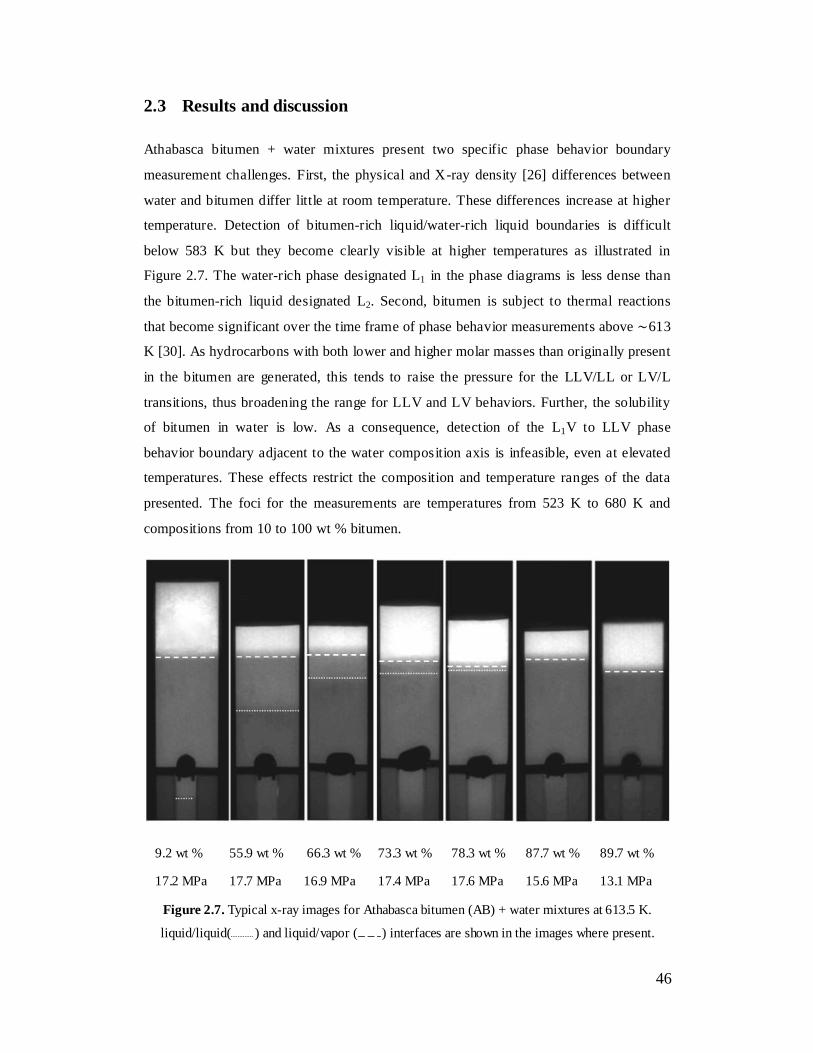
46
2.3 Results and discussion
Athabasca bitumen + water mixtures present two specific phase behavior boundary
measurement challenges. First, the physical and X-ray density [26] differences between
water and bitumen differ little at room temperature. These differences increase at higher
temperature. Detection of bitumen-rich liquid/water-rich liquid boundaries is difficult
below 583 K but they become clearly visible at higher temperatures as illustrated in
Figure 2.7. The water-rich phase designated L1 in the phase diagrams is less dense than
the bitumen-rich liquid designated L2. Second, bitumen is subject to thermal reactions
that become significant over the time frame of phase behavior measurements above ∼613
K [30]. As hydrocarbons with both lower and higher molar masses than originally present
in the bitumen are generated, this tends to raise the pressure for the LLV/LL or LV/L
transitions, thus broadening the range for LLV and LV behaviors. Further, the solubility
of bitumen in water is low. As a consequence, detection of the L1V to LLV phase
behavior boundary adjacent to the water composition axis is infeasible, even at elevated
temperatures. These effects restrict the composition and temperature ranges of the data
presented. The foci for the measurements are temperatures from 523 K to 680 K and
compositions from 10 to 100 wt % bitumen.
9.2 wt %
17.2 MPa
55.9 wt %
17.7 MPa
66.3 wt %
16.9 MPa
73.3 wt %
17.4 MPa
78.3 wt %
17.6 MPa
87.7 wt %
15.6 MPa
89.7 wt %
13.1 MPa
Figure 2.7. Typical x-ray images for Athabasca bitumen (AB) + water mixtures at 613.5 K.
liquid/liquid( ) and liquid/vapor ( ) interfaces are shown in the images where present.

47
Pressure–temperature phase diagrams at fixed composition for Athabasca bitumen +
water mixtures at 9.2, 55.9, 66.3, 73.3, 78.3, 87.7, 88.7 and 96.6 wt % Athabasca bitumen
are shown in Figure 2.8a–h. Phase behavior observations and phase behavior boundary
pressures are reported in Table 2.5. The vapor pressure curve for water is also shown in
Figure 2.8a–h. Like water + pure hydrocarbon binary mixtures, LLV phase behavior
arises in the Athabasca bitumen + water pseudo binary at or above the vapor pressure of
water and the water vapor pressure provides a lower bound for possible LLV phase
behavior. At room temperature, the mutual solubilities of water and hydrocarbons
typically fall into the parts per million to parts per thousand range. At higher
temperatures, the solubility of water in hydrocarbon liquids typically increases sharply
while the solubility of large hydrocarbons in water remains low on a mass basis [31–34].
The phase diagrams for water + Athabasca bitumen reflect these effects. At 523 K and
below, Athabasca bitumen + water mixtures exhibit LLV phase behavior for
compositions ranging from 9.2 to 97 wt % bitumen over a narrow pressure range just
above and well approximated by the vapor pressure of water. At higher temperatures, the
pressure range for LLV phase behavior broadens but the lower pressure bound remains
well approximated as the vapor pressure of water. Hydrocarbon-rich liquid + vapor (L2V)
phase behavior is observed below the LLV region, and a liquid–liquid region arises above
the LLV region in all cases. As the critical temperature of water (647 K) is approached,
there is no qualitative change in this behavior for mixtures comprising 9.2–73.3 wt %
bitumen as shown in Figure 2.8a–d. For 78.3–96.6 wt % bitumen, Figure 2.8e–h, the LLV
region was observed to possess an upper temperature bound that reflects the increasing
solubility of water in the Athabasca bitumen and L2V/ L2 phase behavior boundaries were
identified at high temperatures for these compositions. The placement of L2/LL phase
behavior boundaries in Figure 2.8e–h is approximate. They were not observed
experimentally. The absence of an observed LLV/ L1V phase behavior transition at high
temperature for 9.2 wt % bitumen, indicates that the solubility of bitumen in water
remains less than 9.2 wt % at 620 K, where as the solubility of water in Athabasca
bitumen is more than 13 wt % at the same temperature. Again, this asymmetric solubility
behavior is consistent with the high-temperature behavior of typical hydrocarbon + water
mixtures.

48

49

50

51
Figure 2.8. Pressure-temperature diagrams for Athabasca bitumen + water mixtures at fixed
Athabasca bitumen wt %: a) 9.2 wt %, b) 55.9 wt %, c) 66.3 wt %, d) 73.3 wt %, e) 78.3 wt %, f)
87.7 wt % wt %, g) 88.7 wt %, h) 96.6 wt %. The water vapor pressure curve is shown in each
figure as a dotted curve ( ) terminating at a critical point designated with a solid circle ( ).
Liquid-vapor and liquid-liquid-vapor equilibrium data, are shown as open circles ( ) and open
triangles ( ) respectively. Points on LV/L and LLV/LL boundaries are shown as solid squares ( )
and ( ), and solid curves ( ) trace the LLV/LL and LV/L boundaries. Boundaries designated
with a dash-dot lines ( ) are illustrative and were not identified experimentally.

52
P − x phase diagrams at constant temperature, Figure 2.9a–c, were constructed as
composites of the phase behavior observations and phase behavior boundaries presented
in Figure 2.8a–h. Some parts of the phase diagrams at 583.2, 623.2 and 644 K, shown in
Figure 2.9a–c respectively, are well-defined on this basis. Other parts of the diagrams are
inferred from fragmentary data available, and from theory. The vapor pressure of water
plays an important role in defining these diagrams. At 583.2 K, Figure 2.9a, the phase
diagram is dominated by an L2V region at low pressure and an LL region at high
pressure. The LLV region is restricted to a well-defined 1 MPa wide band above the
vapor pressure of water. The L2V/ L2 phase behavior boundary is also well-defined. The
other phase behavior boundaries (LL/ L1, LLV/ L1V, L2V/V, L1V/V) are qualitative as the
pressure–composition relationships for them are poorly defined. At 623.2 and 644 K,
Figure 2.9b and c, the phase diagrams are qualitatively similar. The pressure range for the
LLV region simply expands, and the composition range for the L2 region broadens.

53
Figure 2.9. Pressure-composition diagrams for Athabasca bitumen + water at fixed temperature:
a) 583.2 K, b) 623.2 K, c) 644 K. Measured liquid-vapor ( ) and liquid-liquid-vapor ( )
equilibrium data are shown. The vapor pressure of water obtained from [27]. Solid lines ( )
show the LL/LLV and L2V/ L2 boundaries where points on these boundaries are designated with
( ) and ( ), respectively, and the L2V/LLV boundary defined by the vapor pressure of water (
). Boundaries designated with a dash-dot lines ( ) are illustrative and were not identified
experimentally.

54
Table 2.5. LLV/LL and L2V/L phase boundaries for Athabasca bitumen + water mixtures
AB (9.2 wt %) + water (90.8 wt %)
T (K) ± 0.1 P (MPa) ± 0.07 Boundary
522.9 4.2 LLV/LL
548.4 6.2 LLV/LL
572.5 8.9 LLV/LL
582.8 10.7 LLV/LL
592.9 12.9 LLV/LL
603.4 16.2 LLV/LL
613.4* 20.2 LLV/LL
623.2* 27.0 LLV/LL
AB (55.9 wt %) + water (44.1 wt %)
T (K) ± 0.1 P (MPa) ± 0.07 Boundary
522.9 4.2 LLV/LL
573.3 9.0 LLV/LL
583.0 10.8 LLV/LL
593.0 12.8 LLV/LL
603.6 16.2 LLV/LL
613.2 20.1 LLV/LL
AB (66.3 wt %) + water (33.7 wt %)
T (K) ± 0.1 P (MPa) ± 0.07 Boundary
523.0 4.2 LLV/LL
548.0 6.0 LLV/LL
573.0 8.7 LLV/LL
583.0 10.7 LLV/LL
593.0 12.7 LLV/LL
602.9 15.7 LLV/LL
613.3 20.2 LLV/LL
623.2* 27.1 LLV/LL

55
AB (73.3 wt %) + water (26.7 wt %)
T (K) ± 0.1 P (MPa) ± 0.07 Boundary
523.1 4.4 LLV/LL
548.2 6.1 LLV/LL
573.4 8.7 LLV/LL
583.3 10.7 LLV/LL
593.2 12.9 LLV/LL
603.6 15.8 LLV/LL
613.5 20.1 LLV/LL
623.1 26.4 LLV/LL
633.9 32.7 LLV/LL
639.2 35.7 LLV/LL
AB (78.3 wt %) + water (21.7 wt %)
T (K) ± 0.1 P (MPa) ± 0.07 Boundary
573.2 9.0 LLV/LL
583.3 10.7 LLV/LL
593.3 12.5 LLV/LL
603.9 15.4 LLV/LL
613.5 20.1 LLV/LL
623.0 25.8 LLV/LL
628.5 27.6 LLV/LL
634.0 28.3 LLV/LL
AB (87.7 wt %) + water (12.3 wt %)
T (K) ± 0.1 P (MPa) ± 0.07 Boundary
522.9 4.1 LLV/LL
553.2 6.7 LLV/LL
573.6 9.1 LLV/LL
583.2 10.6 LLV/LL
593.3 12.7 LLV/LL
603.7 15.9 LLV/LL
613.6 20.1 LLV/LL
623.4 24.2 LV/L

56
633.8 26.2 LV/L
643.9 28.6 LV/L
AB (89.7 wt %) + water (10.3 wt %)
T (K) ± 0.1 P (MPa) ± 0.07 Boundary
523.0 4.2 LLV/LV
548.3 6.2 LLV/LV
573.0 9.1 LLV/LV
583.2 10.7 LLV/LV
593.1 12.8 LLV/LV
603.4 15.4 LLV/LV
613.5 17.6 LV/L
623.1 19.9 LV/L
633.6 21.4 LV/L
644.0 23.0 LV/L
AB (96.6 wt %) + water (3.4 wt %)
T (K) ± 0.1 P (MPa) ± 0.07 Boundary
522.1 4.3 LLV/LL
548.0 5.6 LV/L
572.9 6.8 LV/L
582.8 7.2 LV/L
593.1 7.1 LV/L
603.7 7.3 LV/L
623.4 7.8 LV/L
642.8 9.2 LV/L
*- Values were reduced to reflect the average experiment times at each temperature.
Water + hydrocarbon binary mixtures exhibit Type II, Type IIIa, or Type IIIb phase
behavior as illustrated in Figure 2.1. For water + heavy hydrocarbon binaries, Type II and
Type IIIb phase behavior are observed [18,19]. These latter phase behavior types are
readily distinguished. For Type II phase behavior to arise, the L1 and L2 compositions
approach one another, and converge at an upper critical end point (L1 = L2 + V) remote
from the critical point of the lighter component. For Type IIIb phase behavior to arise, the

57
L1 and L2 phases possess differing compositions up to a K-point (L1 = V + L2) near the
critical point of lighter component. L1 and L2 do not become critically identical. From
Figure 2.9a and b, the composition difference between saturated L1 and L2 phases is large
and changes slowly with temperature. The difference exceeds 90 wt % Athabasca
bitumen at 583.2 K (Figure 2.9a) and exceeds 80 wt % Athabasca bitumen at 623.2 K
(Figure 2.9b). Further, LLV phase behavior is observed at 644 K (Figure 2.9c), just below
the critical temperature of water (647 K), where the mass fraction of Athabasca bitumen
in the L2 phase exceeds 80 wt %. Thus the presence of an upper critical end point (L1 = L2
+ V) is improbable. As the L1 and V phases possess nominally similar water rich
compositions, and the experimental condition is within 3 K of the critical temperature of
water, a K-point is probable. Thus even though a K-point (L1 = V + L2) was not observed
the phase behavior of Athabasca bitumen + water mixtures is consistent with Type IIIb
phase behavior. A pressure–temperature projection and a series of pressure–composition
diagrams at fixed temperature corresponding to this case are shown in Figure 2.10. A
rapid succession of phase diagrams is anticipated as the critical temperature of water is
approached and exceeded.
Figure 2.10. Schematic pressure-temperature projection and pressure-composition at fixed
temperature phase diagrams for the Athabasca bitumen + water pseudo binary mixture. Pure
component vapor pressure curves ( ), liquid-gas (L=V) and liquid-liquid (L=L) critical loci (
), liquid-liquid vapor curve ( ), L=V and L=L critical points ( ) and K-point ( ).

58
Thermal reaction of Athabasca bitumen was detected as an increase in pressure with time
at fixed volume and temperature, as shown in Figure 2.11. Reported pressures and hence
phase behavior boundaries were not corrected for this effect, except as noted in Table 2.5.
Based on the duration of experiments (about one hour at each temperature) and the rate of
pressure rise at fixed temperature, L2V/L and LLV/LL boundaries are over estimated by
at most 1% at 613 K and 16% at 644 K. Experiments were not conducted at higher
temperatures, in part because of the impact of thermal reaction on outcomes, and in part
because water was corroding the interior surfaces of the view cell. While these effects are
not insignificant, they are not expected to affect the phase behavior type designation for
the Athabasca bitumen + water mixture.
Figure 2.11. Thermal reaction rates for 9.2 ( ) and 66.3 ( ) wt % Athabasca bitumen + water
mixtures.
Upcoming contributions will address the solubility of water in the bitumen-rich liquid
phase, volume of mixing and the impact of diluent addition on the phase behavior of
bitumen + water mixtures.
2.4 Conclusion
The phase behavior of Athabasca bitumen + water mixtures was investigated from, 9.2 to
96.6 wt % Athabasca bitumen, over the temperature interval 522.1–644 K, and the
pressure interval 4.2–35.7 MPa. The apparatus and procedures were validated using
known properties of pure fluids and binary mixtures where reported phase boundary

59
temperatures, pressures, and compositions were reproduced to within 0.5 K, 0.2 MPa, 0.1
wt % respectively for water + toluene and water + 1-methylnaphthalene binary mixtures
from 453 to over 573 K. Pressure–temperature at fixed composition and pressure–
composition at fixed temperature phase diagrams were prepared for the Athabasca
bitumen + water pseudo binary mixture. Based on the composition difference between the
water-rich and the Athabasca bitumen-rich liquid phases, the trend in this difference with
temperature, and the observation of LLV phase behavior adjacent to the critical point of
water, the phase behavior designation Type IIIb according to the van Konynenburg and
Scott classification scheme is assigned to the mixture. Thermal reaction of Athabasca
bitumen impacts the phase boundary pressures at temperatures exceeding 620 K but does
not appear to impact the phase behavior type designation for the mixture.
2.5 References
[1] A. Kruse, E. Dinjus, Hot compressed water as reaction medium and reactant-2.
Degradation reactions, Journal of Supercritical Fluids 41 (2007) 361–379.
[2] A. Kruse, E. Dinjus, Hot compressed water as reaction medium and reactant –
properties and synthesis reactions, Journal of Supercritical Fluids 39 (2007) 362–
380.
[3] L.-n. Han, R. Zhang, J.-c. Bi, Upgrading of coal-tar pitch in supercritical water,
Journal of Fuel Chemistry and Technology 36 (2008) 1–5.
[4] T. Sato, T. Adschiri, K. Arai, G.L. Rempel, F.T.T. Ng, Upgrading of asphalt with
and without partial oxidation in supercritical water, Fuel 82 (2003) 1231–1239.
[5] L.N. Han, R. Zhang, J.C. Bi, Experimental investigation of high-temperature coal
tar upgrading in supercritical water, Fuel Processing Technology 90 (2009) 292–
300.
[6] Z.M. Cheng, Y. Ding, L.Q. Zhao, P.Q. Yuan, W.K. Yuan, Effects of supercritical
water in vacuum residue upgrading, Energy and Fuels 23 (2009) 3178–3183.
[7] M. Morimoto, Y. Sugimoto, Y. Saotome, S. Sato, T. Takanohashi, Effect of
supercritical water on upgrading reaction of oil sand bitumen, The Journal of
Supercritical Fluids 55 (2010) 223–231.
[8] M. Watanabe, S.-n. Kato, S. Ishizeki, H. Inomata, R.L. Smith Jr., Heavy oil
upgrading in the presence of high density water: basic study, The Journal of
Supercritical Fluids 53 (2010) 48–52.

60
[9] W. Wahyudiono, T. Shiraishi, M. Sasaki, M. Goto, Bitumen upgrading under
solvothermal/hydrothermal conditions, Research on Chemical Intermediates 37
(2011) 375–381.
[10] K. Arai, T. Adschiri, Importance of phase equilibria for understanding supercrit -
ical fluid environments, Fluid Phase Equilibria 158–160 (1999) 673–684.
[11] T.W. De Loos, A.J.M. Wijen, G.A.M. Diepen, Phase equilibria and critical
phenomena in fluid (propane + water) at high pressures and temperatures, The
Journal of Chemical Thermodynamics 12 (1980) 193–204.
[12] T.W. De Loos, W.G. Penders, R.N. Lichtenthaler, Phase equilibria and critical
phenomena in fluid (n-hexane + water) at high pressures and temperatures, The
Journal of Chemical Thermodynamics 14 (1982) 83–91.
[13] T.W. De Loos, J.H. van Dorp, R.N. Lichtenthaler, Phase equilibria and critical
phenomena in fluid (n-alkane + water) systems at high pressures and temper-
atures, Fluid Phase Equilibria 10 (1983) 279–287.
[14] T. Yiling, T. Michelberger, E.U. Franck, High-pressure phase equilibria and crit-
ical curves of (water + n-butane) and (water + n-hexane) at temperatures to 700 K
and pressures to 300 MPa, The Journal of Chemical Thermodynamics 23 (1991)
105–112.
[15] Q. Wang, K.-C. Chao, Vapor–liquid and liquid–liquid equilibria and critical states
of water + n-decane mixtures, Fluid Phase Equilibria 59 (1990) 207–215.
[16] R.L. Stevenson, D.S. LaBracio, T.A. Beaton, M.C. Thies, Fluid phase equilibria
and critical phenomena for the dodecane–water and squalane–water sys-tems at
elevated temperatures and pressures, Fluid Phase Equilibria 93 (1994) 317–336.
[17] S.P. Christensen, M.E. Paulaitis, Phase equilibria for tetralin–water and 1-
methylnaphthalene–water mixtures at elevated temperatures and pressures, Fluid
Phase Equilibria 71 (1992) 63–83.
[18] E. Brunner, Fluid mixtures at high pressures IX. Phase separation and critical
phenomena in 23 (n-alkane + water) mixtures, The Journal of Chemical Ther-
modynamics 22 (1990) 335–353.
[19] E. Brunner, M.C. Thies, G.M. Schneider, Fluid mixtures at high pressures: phase
behavior and critical phenomena for binary mixtures of water with aromatic
hydrocarbons, The Journal of Supercritical Fluids 39 (2006) 160–173.
[20] P.H. Vankonynenburg, R.L. Scott, Critical lines and phase-equilibria in binary
vanderwaals mixtures, Philosophical Transactions of the Royal Society of Lon-
don. Series A. Mathematical Physical and Engineering Sciences 298 (1980) 495–
540.

61
[21] A. Bazyleva, M. Fulem, M. Becerra, B. Zhao, J.M. Shaw, Phase behavior of
Athabasca bitumen, Journal of Chemical and Engineering Data 56 (2011) 3242–
3253.
[22] M.R. Gray, P. Jokuty, H. Yeniova, L. Nazarewycz, S.E. Wanke, U. Achia, A.
Krzy-wicki, E.C. Sanford, O.K.Y. Sy, The relationship between chemical-
structure and reactivity of Alberta bitumens and heavy oils, Canadian Journal of
Chemical Engineering 69 (1991) 833–843.
[23] O.P. Strausz, E.M. Lown, A. Morales-Izquierdo, N. Kazmi, D.S. Montgomery,
J.D. Payzant, J. Murgich, Chemical composition of Athabasca bitumen: the
distill-able aromatic fraction, Energy and Fuels 25 (2011) 4552–4579.
[24] X.Y. Zou, X.H. Zhang, J.M. Shaw, Phase behavior of Athabasca vacuum bottoms
plus n-alkane mixtures, SPE Production and Operation 22 (2007) 265–272.
[25] X.H. Zhang, The Impact of Multiphase Behavior on Coke Deposition in Heavy
Oil Hydroprocessing Catalysts, University of Alberta, Edmonton, 2006.
[26] S.J. Abedi, H.Y. Cai, S. Seyfaie, J.M. Shaw, Simultaneous phase behaviour, ele -
mental composition and density measurement using X-ray imaging, Fluid Phase
Equilibria 158 (1999) 775–781.
[27] E.W. Lemmon, M.O. McLinden, D.G. Friend, Thermophysical properties of fluid
systems, in: P.J. Linstrom, W.G. Mallard (Eds.), NIST Chemistry WebBook,
NIST Standard Reference Database Number 69, National Institute of Standards
and Technology, Gaithersburg MD, 2012.
[28] F.E. Anderson, J.M. Prausnitz, Mutual solubilities and vapor-pressures for binary
and ternary aqueous systems containing benzene, toluene, meta-xylene, thio-
phene and pyridine in the region 100–200 ◦C, Fluid Phase Equilibria 32 (1986)
63–76.
[29] K. Chandler, B. Eason, C.L. Liotta, C.A. Eckert, Phase equilibria for binary
aqueous systems from a near-critical water reaction apparatus, Industrial and
Engineer-ing Chemistry Research 37 (1998) 3515–3518.
[30] H.Y. Cai, J.M. Shaw, K.H. Chung, Hydrogen solubility measurements in heavy
oil and bitumen cuts, Fuel 80 (2001) 1055–1063.
[31] I.G. Economou, J.L. Heidman, C. Tsonopoulos, G.M. Wilson, Mutual solubilities
of hydrocarbons and water.3. 1-hexene, 1-octene C-10-C-12 hydrocarbons,
AIChE Journal 43 (1997) 535–546.
[32] J.L. Heidman, C. Tsonopoulos, C.J. Brady, G.M. Wilson, High-temperature
mutual solubilities of hydrocarbons and water. 2. Ethylbenzene,
ethylcyclohexane, and normal-octane, AIChE Journal 31 (1985) 376–384.
62
[33] C. Tsonopoulos, Thermodynamic analysis of the mutual solubilities of hydro-
carbons and water, Fluid Phase Equilibria 186 (2001) 185–206.
[34] C. Tsonopoulos, Thermodynamic analysis of the mutual solubilities of normal
alkanes and water, Fluid Phase Equilibria 156 (1999) 21–33.
[35] D.-Y. Peng, D.B. Robinson, A new two-constant equation of state, Industrial and
Engineering Chemistry Fundamentals 15 (1976) 59–64.

63
Chapter 3. Volume of mixing and solubility of water in
Athabasca bitumen at high temperature and pressure1
3.1 Introduction
The Phase behavior, mutual solubility and other physical property data for water +
hydrocarbon mixtures are necessary for the development, design and optimization of a
variety of high temperature industrial processes such as bitumen production and
upgrading (Chapter 2, [1]). The properties of mixtures of water + Athabasca bitumen and
other heavy hydrocarbons are of growing interest because water, at high temperature,
provides a reaction medium for upgrading heavy hydrocarbons [2-10] that may prove to
be preferred over conventional hydrocarbon based ones. In addition to upgrading
applications, the solubility and volume of mixing of water in heavy hydrocarbon
resources are essential to the development of production models for oil and bitumen
production processes such as the Steam Assisted Gravity Drainage (SAGD) method
where net water consumption, and water recycling present both environmental and
economic challenges [11]. This study was also motivated by the potential to reduce the
overall cost of production of finished products in the future by merging aspects of fluid
composition and operating conditions for in situ production and upgrading processes. For
example, water is already used in production and the solvent properties and solubility of
water in the near-critical region make it an efficient medium for carrying out chemica l
reactions, and the changes of water solubility with temperature and pressure may
facilitate subsequent water-hydrocarbon separation and water reuse.
The thermophysical properties and phase behavior of water-hydrocarbon mixtures at
high-temperature have received limited attention and there are few benchmark data sets
available to underpin industrial process design, development or optimization. Data are
available for a limited number of pure hydrocarbon + water and hydrocarbon mixture +
water cases. Maczynski et al. [12-23] reviewed and critically compiled the published data
for mutual solubilities of C5-C36 hydrocarbons + water/seawater mixtures. Their
compilation provides a comprehensive collection of mutual binary solubility data over a
broad range of temperatures. Brown et al. [24] provide solubility data for binary mixtures
1 This chapter with minor modifications has been published in the journal of Fluid Phase
Equilibria: M. J. Amani, M. R. Gray, and J. M. Shaw, Fluid Phase Equilibria, DOI:
10.1016/j.fluid.2013.07.021.

64
of water with acetophenone, anisole, 1-octanol and toluene in the temperature range of
370 K to 550 K. Tsonopoulos et. al [25-30] measured and correlated mutual solubility
data for hydrocarbon + water binaries under three phase liquid-liquid-vapor equilibrium
conditions up to their upper critical end points (UCEP) where for example, the phase
compositions of both liquid phases for homologous series of alkanes, alkyl cyclohexanes,
1-alkenes, and alkyl benzenes at high temperatures are reported [30]. Chandler [31]
reported the mutual solubilities of toluene + water and benzene + water up to 473 K along
the LLV three-phase curve up to a pressure of 17.2 MPa. Anderson et al. [32]
investigated the mutual solubilities and vapor pressures for four binary and one ternary
aqueous mixture. Leet et al. [33] studied the mutual solubilities of water and six
polycyclic aromatic hydrocarbons including N-, O-, and S-containing polycyclic
aromatics at high temperatures. Neely et al. [34] measured the mutual hydrocarbon–water
liquid-liquid equilibrium data for mixtures comprising the benzene, toluene, and 3-
methylpentane in a temperature range from ambient temperature up to 500 K. Brunner
[35, 36] studied the phase behavior and critical phenomena of water + n -alkanes binary
mixtures (up to n-eicosane) and water + aromatic compounds at pressures and
temperatures exceeding the critical point of water. Phase equilibrium measurements for
water + tetralin and 1-methylnaphthalene, up to 673.2 K, are also available [37]. Phase
equilibrium data for reservoir fluids, including water, are very scarce. De Hemptinne et
al. [38] investigated the phase equilibria of petroleum fractions + water mixtures and
Pedersen [39] reported equilibrium compositions, three-phase equilibrium pressure and
temperatures for water + petroleum reservoir fluids up to 473 K.
High-temperature experimental phase density and excess volume data for hydrocarbon +
water mixtures are limited to a few studies. Abdulagatov et al. [40-45] conducted
measurements for water + n-pentane to n-octane, and water + benzene at temperatures
near the critical point of water and report liquid phase thermodynamic properties and
partial molar volumes. Furutaka et al. [46-50] measured compositions and densities of
hydrocarbon-rich phases at equilibrium for water + benzene, toluene, ethylbenzene, n -
hexane and n-decane mixtures in the vicinity of the upper end critical point of these
mixtures using infrared spectroscopy. Their work focused on unsaturated hydrocarbon-
rich phases at pressures above the LLV three-phase curve. They report large and positive
volumes of mixing for hydrocarbon-rich liquids. Hnedkovsky et al. [51, 52] present phase
density and partial molar volume data of hydrocarbons at infinite dilution for water-rich

65
liquid phases where the hydrocarbons include benzene, toluene, and cresols over the
temperature interval 298.15 to 573.15 K.
Figure 3.1. Type IIIb pressure-temperature projection for water + hydrocarbon binary mixtures. (
) critical points for the water and the hydrocarbon, and ( ) the UCEP for the mixture. ( ) and
( ) are the critical locus and LLV three-phase curve respectively and ( ) denotes vapor/bubble
pressure curves (Chapter 2).
In our prior work we showed that the Athabasca bitumen + water pseudo binary mixture
exhibits Type IIIb phase behavior (Chapter 2) according to the naming scheme of van
Konynenburg and Scott [53].Type IIIb phase behavior occurs because for this
hydrocarbon + water mixture the hydrocarbon crit ical temperature is much higher than
the critical temperature of water [35, 36]. The key characteristics of Type IIIb phase
behavior are illustrated in Figure 3.1. The LLV three-phase equilibrium curve extends
from low temperature up to the vicinity of the critical point of water where it is
intersected by the liquid-vapor critical locus extending from the critical point of water.
This intersection, the upper critical point (UCEP), is where the water -rich liquid and
vapor phases become critically identical. Above the UCEP temperature a maximum of
two phases arise in the phase diagram. This phase behavior contrasts with the behavior of
typical hydrocarbon + water mixtures, available in the literature, which exhibit Type II or
Type IIIa phase behavior as discussed previously in Chapter 2. For Type IIIa phase
behavior, the hydrocarbon-rich phase becomes critically identical to the vapor phase at
the upper critical end point. At low temperatures, the properties of Type IIIa and Type

66
IIIb binary mixtures differ little but they are expected to diverge at high temperatures.
The high temperature properties of the hydrocarbon-rich liquid phase are the focus of the
current study where phase compositions, and excess volumes for model hydrocarbon +
water mixtures are used to benchmark measurements for water + Athabasca bitumen
mixtures and to place them in a broader context.
3.2 Experiments and methodology
d Athabasca bitumen, provided by Syncrude Canada Ltd, Alberta, Canada, was produced
by a commercial froth treatment process. SARA analysis for Athabasca bitumen is
presented in Chapter 2 and [54]. The properties of used water, toluene and 1-
methylnaphthalene are described in Chapter 2.
A schematic of the X-ray view cell is shown in Figure 3.2. Detailed descriptions of the
apparatus and operating procedures, along with illustrative applications have been
reported in a series of recent publications [55-57]. In brief, the view cell consists of a
beryllium cylinder with an approximate total internal volume of 200 cm3. The upper end
cap includes a variable volume bellows and the view cell volume is controlled by back
pressuring the bellows using high-pressure nitrogen. The cell is equipped with a magnet
stirrer resting on the fixed lower end cap, and feed lines allow for both gas and liquid
injection and air removal once the cell is assembled. More details can be find in Chapter
2. In this work, the cell volume was carefully calibrated and digital images were
processed to identify interface elevations and hence phase volumes. This approach was
found to be more accurate than calibrating transmitted x-ray intensity with phase density.
The experimental approach, and calibration and operation procedures were validated by
reproducing published experimental and recommended water, 1-methylnaphthalene, and
water + toluene and water + 1-methylnaphthalene binary mixtures properties.

67
Figure 3.2. The X-ray view cell schematic. The view-cell is equipped with a variable volume
bellows and a magnetic stirrer.
3.2.1 Water solubility measurement validation
Reliable measurement of mutual solubilities is challenging at elevated temperatures and
pressures, and analysis of the phase compositions at equilibrium is subject to large errors
[32]. To avoid the difficulties associated with sampling and subsequent analysis,
experimentally measured points on the LV-L boundary that are close to the LLV
boundary are extrapolated linearly to the experimentally identified LLV three phase
pressure as illustrated in Figure 3.3a (mass basis) and Figure 3.3b (mole basis) for water
+ tetralin at 573.2 K [37]. These pressure-composition (at fixed temperature) diagrams
are typical for Type II and Type III phase behaviors at temperatures below the UCEP and
the approach, illustrated on both a mole and a mass basis, is akin to Luks’ conjugate pair
approach [58] for phase boundary identification. Here, points on the hydrocarbon-rich
LV-L boundary are extrapolated to the intersection with the LL-LLV boundary. The
composition at the point of intersection is the water-saturated hydrocarbon-rich liquid
phase composition. This composition determines the maximum fraction or solubility of
water in the hydrocarbon-rich phase. As high-temperature and high-pressure phase
behavior measurements are time consuming, costly, and challenging, only a few LV-L
transition points can be measured in practice. The difference between measured and
extrapolated solubilities is minimized if LV-L transition data are available close to the
solubility limit.

68
Figure 3.3. P-x diagrams for tetralin + water at 573.2 K: (a) mass-based and (b) mole-based. The
experimental data ( ) and the three-phase line ( ) are from Christensen [37] and ( ) is the
estimated composition of the saturated tetralin-rich liquid.
This experimental approach was validated by reproducing water solubility in
hydrocarbon-rich liquid data for the water + toluene and water + 1-methylnaphtalene
binary mixtures. These experimental solubility results, based on as few as 2 LV-L
transition points (including the pure hydrocarbon vapor pressure) per solubility
measurement, are reported in Tables 3.1 and 3.2. The data, obtained in this manner, fall
within the scatter of the literature data as shown in Figure 3.4. While precise
measurement is unlikely, the quality of the results obtained using this indirect and non -

69
intrusive technique under extreme conditions vis-à-vis more complex approaches is
encouraging from a technique development perspective. These validat ion results may also
contribute to, but cannot resolve debates on the relative merits of compiled [21] versus
measured experimental [26] data for water solubility in 1-methylnaphthalene at high
temperature.
Table 3.1. Water solubility in toluene (wt %)
T (K) wt % # of LV-L points
513.1 7.5 ± 0.6 6
533.1 11.5 ± 1.3 4
553.2 19.0 ± 2.5 2
Table 3.2. Water solubility in 1-methylnaphthalene (wt %)
T (K) wt % # of LV-L points
533.3 5.7 ± 0.9 2
553.6 7.4 ± 1.4 2
573.2 13.6 ± 3.0 3
3.2.2 Liquid density measurement validation
As water was used to calibrate view-cell volume and the density of 1-methylnaphthalene
is closer to that of bitumen + water mixtures than toluene, 1-methylnaphthalene was used
for density measurement validation. The results are presented and compared to NIST
recommended values [59] in Table 3.3. The two sets of values agree to within 5 kg/m3 on
average over the temperature interval 326.5 to 573.8 K. It is worth noting that the
uncertainty of the NIST recommended values increases sharply with temperature,
especially above 470 K. The uncertainty of the digital measurements reported here
declines with increasing temperature, because the uncertainty is linked primarily to the
height of an individual pixel (fixed) in a digital image divided by the number of pixe ls
(proportional to volume which increasing with temperature). Thus the validation data
reduce the uncertainty and improve the confidence limits for 1-methylnaphthalene liquid
density measurements at high temperatures.

70
Figure 3.4. The solubility of water in: a) toluene (this work ( ), Anderson et al. [32] ( ), Brown et
al. [24] ( ), Chandler et al. [31] ( ), Jou et al. [65] ( ) and Neely et al. [34] (+)) and in b) 1-
methylnaphthalene (this work ( ), Economou et al. [26] ( ), Christensen et al. [37] ( ), and
compilation of the former data by Shaw et al. [21] ( )).

71
Table 3.3. Saturated density of liquid 1-methylnaphthalene (kg/m3)
T (K) This work NIST [59]
326.5 1001 ± 13 994.3 ± 1.1
341.9 984 ± 13 982.7 ± 1.3
370.7 967 ± 12 961.4 ± 1.9
396.4 949 ± 12 942.4 ± 2.8
420.9 926 ± 11 924.2 ± 3.7
447.4 902 ± 11 903.9 ± 4.9
472.4 874 ± 10 884.1 ± 6.8
498.2 852 ± 9 863 ± 10
522.3 828 ± 9 841 ± 16
547.5 812 ± 8 817 ± 25
573.8 787 ± 8 790 ± 37
3.3 Results and discussion
3.3.1 Solubility of water in bitumen
Pressure – composition diagrams at 523.0 K, 548.2 K, 573.1 K, 583.2 K, 593.1 K, 603.5
K, 613.4 K, 623.2 K, 633.8 K, 644.0 K for Athabasca bitumen + water mixtures,
presented and described in detail in Chapter 2, are reproduced as Figures 3.5a-j so that the
method for determining water solubility in bitumen is apparent. In Figures 3.5a-g, the
solubility was determined from a minimum of five points defining the LLV-LL transition
and two points defining the LV-L transition. On the scale of the Figures, the bubble
pressure of the Athabasca bitumen is negligible. At higher temperatures, Figures 3.5h-j,
there are fewer points defining the LLV-LL transition and more defining the LV-L
transition. Above 600 K thermal degradation of Athabasca bitumen affects mixture
composition and increases the apparent bubble pressure as a consequence of light
hydrocarbon formation. Rates of pressure rise with time were measured and bubble
pressures were found to be overestimated by approximately 1% at 613 K and 16% at 644
K based on the duration of experiments. Reported pressures were corrected for this effect.
Solubility values for water in Athabasca bitumen, along with their uncertainty are
reported in Table 3.4 and are shown in the context of available solubility data for water in

72
other pertinent pure and mixed hydrocarbons in Figure 3.6a. Water solubility in
Athabasca bitumen is approximately one order of magnitude lower than in low molar
mass hydrocarbons such as toluene irrespective of temperature.

73

74

75

76
Figure 3.5. Pressure-composition diagrams for Athabasca bitumen + water at fixed temperature:
(a) 523.0 K (b) 548.2 K, (c) 573.1 K, (d) 583.2 K, (e) 593.1 K, (f) 603.5 K, (g) 613.4 K, (h) 623.2
K, (i) 633.8 K, (j) 644. Measured liquid-vapor ( ) and liquid-liquid-vapor ( ) equilibrium data are
shown. The vapor pressure of water obtained from [59]. Solid lines ( ) show the LL/LLV and
L2V/L2 boundaries where points on these boundaries are designated with ( ) and ( ),
respectively, and the L2V/LLV boundary defined by the vapor pressure of water ( ). Boundaries
designated with a dash-dot lines ( ) are illustrative and were not identified experimentally.

77
Figure 3.6. Solubility of water in Athabasca bitumen, this work ( ), and in other hydrocarbons: a)
all available hydrocarbons:, b) high molar mass compounds and heavy oils, and equation 3-1 ( )
. Symbols: toluene ( ) [24, 31, 32], ethylbenzene ( ) [27], m-xylene (+) [32], ethylcyclohexane (-
) [27], n-octane ( ) [27], tetralin ( ) [26], 1,2,3,4-Tetrahydroquinoline [33], thianaphthene ( )
[33], cis-decalin ( ) [26], 1-butylcyclohexane ( )[26], decane ( )[26], 1-methylnaphthalene ( )
[26], 1-ethylnaphthalene ( ) [26], 1,4-diisopropylbenzene ( ) [26], 9,l0-dihydrophenanthrene ( )
[33], naphtha ( , Mw = 147) [60], kerosene(×,Mw = 173) [60], lubricating oil ( , Mw = 425)
[60], gross oil mixtures ( , Mw = 425) [63], Coalinga crude oil (|, Mw = 439) [61],Huntington
Beach crude oil ( , Mw = 442) [61],Peace River crude oil ( , Mw = 571) [61] Cat Canyon crude
oil ( , Mw = 627) [61] .

78
Table 3.4. Solubility of water in the bitumen-rich liquid phase.
T (K) wt % uncertainty (wt %)
548.2 3.7 1.1
573.1 5.3 1.5
583.2 6.2 1.8
593.1 7.7 2.2
603.5 8.8 2.2
613.4 11.3 1.2
623.2 13.5 1.1
633.8 15.2 1.4
644 16.9 1.5
Table 3.5. Density of Athabasca bitumen
T (K) Density (kg/m3) uncertainty (kg/m3)
377.2 986.6 9.5
399.8 976.7 9.3
422.8 963.7 9.0
446.9 943.8 8.6
472.0 929.7 8.4
492.3 917.9 8.2
513.4 906.5 8.0
533.4 895.3 7.8
552.6 881.7 7.6
571.3 871.1 7.4
594.2 855.6 7.1
603.5 850.6 7.0
614.0 840.8 6.9
624.2 833.5 6.8
633.8 824.0 6.6
643.5 814.8 6.5

79
The data in this work extend the existing water in hydrocarbon solubility data set for
heavy hydrocarbon mixtures of industrial importance up to the critical point of water. The
data are also well aligned with water solubility data in high-molar mass polynuclear
aromatic compounds, lubricating oil [60], Coalinga crude oil, Huntington Beach crude oil
and Peace River crude oil [61] where the data sets overlap or abut, as shown in Figure
3.6b. However, it would appear that from the temperature dependence of the solubilities
reported in the work of Glandt and Chapman [60] that the low temperature solubilities for
the fluids they measured are overstated. The temperature trends in their data do not align
with other measurements.
From the perspective of process design and optimization, interpolation and extrapolation
of water solubility in the hydrocarbon-rich liquid and hydrocarbon solubility in water-rich
liquid are important topics. Both of these topics present significant challenges related to
the quality and range of the underlying solubility data, the diversity of the underlying
phase behaviors represented in the data sets, and hydrocarbon speciation. These
challenges are addressed elsewhere [62] in detail. Here the log-linear behavior of water
solubility in hydrocarbons, Figure 3.6a, on a mass basis is exploited to provide a first
order estimate for water solubility in heavy hydrocarbons, including lubricating oil and
Athabasca bitumen. Equation 3-1 tracks the low solubility limit of the experimental data.
The coefficients appearing in equation 1 were regressed using water solubility data in
Athabasca bitumen, gross oil mixture [63] and lubrication oil [60]:
( 3-1)
where mw is the water mass fraction in the hydrocarbon-rich liquid phase, and T is
temperature in K. The constants are A = 2.019*10-07 and B = 2.155*10-02 (1/K), and the
average absolute relative deviation of the correlation relative to the data, 12.3%, falls
within the uncertainty of the underlying data which ranges up to 30%.
3.3.2 Excess volume of the Athabasca bitumen-rich liquid phase
Measured density data for saturated Athabasca bitumen liquid, presented in Table 3.5,
were regressed using the Rackett equation [64] :
] ( 3-2)

80
where is the density of Athabasca bitumen in kg/m3, C = 1.586, D = 1.065*103, E =
2.857*10-1, F = 5.493 and T is absolute temperature in K to obtain smoothed density
values. The average absolute deviation of equation 3-2 from the density data is 2.6 kg/m3.
Excess volume values were then calculated on a mass basis from experimental phase
density and composition data as:
( 3-3)
where is the excess volume of the bitumen-rich liquid phase. mw and mAB are the
mass fraction of water and Athabasca bitumen in the mixture, and and are the
smoothed saturated liquid densities obtained from NIST [59] for water and equation 3-2
for Athabasca bitumen. The saturated liquid densities were not corrected for pressure
where the pressure is less than vapor pressure of water. The water is slightly less dense
and the Athabasca bitumen slightly more dense at the pressures where the excess volumes
are evaluated. As these trends compensate, the net impact on the excess volume
calculations is expected to be small but the effect is variable and contributes to the
uncertainty of the values. Thus the excess volume values reported in Table 3.6 must be
viewed as approximate. However, the values are positive, as is expected for water +
hydrocarbon mixtures.
Figure 3.7. A typical volume of mixing for heavy hydrocarbon + water at temperatures lower than
the upper critical end point.

81
For mixtures exhibiting liquid-liquid behavior, excess volume increases from zero to a
maximum at the liquid-liquid boundary, is a linear function of composition in the two-
phase region and then decreases to zero in the second single-phase liquid region, as
shown in Figure 3.7. One way to interpret the excess volume measurements is suggested
by Figure 3.7. If excess volume is treated as a linear function of composition within the
single-phase region, each excess volume measurement can also be treated as an
approximate measure of ∆VE/mw. As the saturated composition is known, the excess
volume for saturated liquid, with uncertainty estimates can be obtained, as shown in
Figure 3.8. The excess volume at a water mass fraction less than the saturated value can
be estimated as:
∆VE = mw *(A*T+B) ( 3-4)
where
∆VE/mw = A*T + B ( 3-5)
Again, mw is the mass fraction of water in the bitumen-rich phase, and T is in K.
Constants A = -1.63*10-5 (m3/kg.K) and B = 1.068*10-2 (m3/kg) are calculated by linear
regression.
Figure 3.8. Excess volume ( ) for the Athabasca bitumen-rich phase at saturation. The line
segments, (------) represent the excess volumes of unsaturated Athabasca bitumen. Temperature is
a parameter.

82
Figure 3.9. The derivative of excess volume with water mass fraction obtained by analyzing
excess volume data for benzene ( ) [46, 47], toluene ( ) [46, 49], ethylbenzene ( ) [46, 49], n-
hexane ( ) [50], n-decane ( ) [50], and for Athabasca bitumen ( ) this work.
To place the behavior of water + Athabasca bitumen mixtures in a broader context,
∆VE/mw values for water in hydrocarbons were derived in a similar manner using
excess volume measurements reported in the literature. Excess volumes for unsaturated
water + benzene, toluene, ethylbenzene, n-hexane, and n-decane mixtures exhibiting
Type IIIa phase behavior, are available at 10 MPa over a range of temperatures [48-50]
near their respective upper critical end points. ∆VE/mw values for these mixtures are
compared with those for water in Athabasca bitumen in Figure 3.9. The phase state
associated with these data is a hydrocarbon-rich liquid (L1) and according to literature
[48-50], these hydrocarbon-rich phases approach their respective critical points (UCEP)
within each data set. For the water + Athabasca bitumen pseudo binary mixture, which
exhibits Type IIIb phase behavior, the reported derivative values are for L2, a
hydrocarbon-rich liquid phase. This phase remains subcritical even as the water critica l
temperature is approached because the critical temperature of Athabasca bitumen is high
relative to that of water. These phase state distinctions are important because the
∆VE/mw values in water + Athabasca bitumen mixtures are low compared to water +
light hydrocarbon mixtures, and possess opposing trends with temperature as the critica l
temperature of water is approached.

83
Table 3.6. Bitumen-rich phase density and excess specific volume data
T (K) P (MPa) Water (wt %)
density of bitumen-rich liquid phase (kg/m
3)
(m3/kg*10
5)
/ water wt
% (m3/kg *10
6)
593.1 5.4 4.0 824.0 3.0 7.4
593.1 12.2 8.1 761.0 11.7 14.5
593.3 11.8 8.1 768.9 10.3 12.7
593.3 12.2 8.1 788.3 7.1 8.8
593.2 12.0 8.1 765.3 10.9 13.5
593.0 12.2 8.1 787.5 7.3 9.1
593.0 11.9 8.1 762.5 11.5 14.2
603.7 5.5 4.0 816.4 2.9 7.2
603.4 13.3 9.4 758.8 10.2 10.9
603.7 14.0 9.4 760.3 9.9 10.5
603.9 14.8 9.5 764.8 9.1 9.6
603.4 14.4 9.4 766.0 9.0 9.6
602.9 14.1 9.3 768.4 8.7 9.3
603.6 13.8 9.4 760.3 10.2 10.8
613.5 14.4 10.2 752.3 9.4 9.2
613.6 16.1 10.8 741.8 11.0 10.1
613.5 17.9 10.8 766.9 6.9 6.3
613.5 17.8 10.8 741.1 11.2 10.4
613.3 17.1 10.8 765.7 7.1 6.5
613.2 16.5 10.8 757.4 8.7 8.1
623.4 6.0 4.0 808.8 1.6 3.9
623.1 14.9 10.2 750.1 7.9 7.8
623.4 17.7 12.3 736.2 9.3 7.5
623.0 19.5 12.3 759.2 5.2 4.2
623.1 20.7 12.4 762.6 5.9 4.8
623.3 21.0 12.4 748.4 8.1 6.5
623.3 22.8 12.4 741.4 9.8 7.9
633.6 16.2 10.2 745.6 7.3 7.2
633.8 19.8 12.3 734.0 9.5 7.7
634.0 765.7 14.3 764.7 3.8 2.7
633.9 26.0 14.3 755.8 5.4 3.8
642.8 6.8 4.0 784.7 1.7 4.2
644.1 17.0 10.2 722.0 5.7 5.5
643.9 20.4 12.3 716.9 4.5 3.7
644.0 26.2 16.2 733.0 4.6 2.8

84
3.4 Conclusion
The solubility of water in Athabasca bitumen and the excess volume of the bitumen-rich
liquid phase are reported over the temperature interval 593.2 to 644 K. The accuracy of
the experimental methods and data were verified by reproducing phase diagrams and
hydrocarbon-rich liquid compositions for water + toluene and water + 1 -
methylnaphthalene, and reproducing density measurements for 1-methylnaphthalene up
to 573.8 K. The impacts of thermal degradation of Athabasca bitumen on measured
values, particularly above 613 K, were mitigated but not eliminated by the experimenta l
methods and procedures. The solubility of water in Athabasca bitumen increases with
temperature. The reported values and the trend with temperature are in agreement with
numerous data sets for comparable hydrocarbons but are at variance with values reported
by Glant and Chapman [60] which appear to overestimate water solubility at lower
temperatures. The excess volumes for the saturated sub-critical bitumen-rich liquid phase
were found to be positive and the values were found to decrease with increasing
temperature. Behaviorial differences arising in Type IIIa and Type IIIb phase diagrams
are delineated.
3.5 References
[1] M.J. Amani, M.R. Gray, J.M. Shaw, Phase behavior of Athabasca bitumen +water
mixtures at high temperature and pressure, Journal of Supercritical Fluids 77
(2013) 142–152.
[2] T. Sato, T. Adschiri, K. Arai, G.L. Rempel, F.T.T. Ng, Upgrading of asphalt with
and without partial oxidation in supercritical water, Fuel 82 (July) (2003) 1231–
1239.
[3] Z. Fang, T. Sato, R.L. Smith Jr., H. Inomata, K. Arai, J.A. Kozinski, Reaction
chemistry and phase behavior of lignin in high-temperature and supercritical water,
Bioresource Technology 99 (2008) 3424–3430.
[4] M. Morimoto, Y. Sugimoto, Y. Saotome, S. Sato, T. Takanohashi, Effect of super -
critical water on upgrading reaction of oil sand bitumen, Journal of Supercritical
Fluids 55 (2010) 223–231.
[5] M. Watanabe, S.-n. Kato, S. Ishizeki, H. Inomata, R.L. Smith Jr., Heavy oil
upgrading in the presence of high density water: basic study, Journal of
Supercritical Fluids 53 (2010) 48–52.

85
[6] L.-N. Han, R. Zhang, J.-C. Bi, Upgrading of coal-tar pitch in supercritical water,
Journal of Fuel Chemistry and Technology 36 (2008) 1–5.
[7] L.N. Han, R. Zhang, J.C. Bi, Experimental investigation of high-temperature coal
tar upgrading in supercritical water, Fuel Processing Technology 90 (February)
(2009) 292–300.
[8] Z.M. Cheng, Y. Ding, L.Q. Zhao, P.Q. Yuan, W.K. Yuan, Effects of supercritical
water in vacuum residue upgrading, Energy & Fuels 23 (May–June) (2009) 3178–
3183.
[9] Z. Fang, R.L. Smith, H. Inomata, K. Arai, Phase behavior and reaction of
polyethylene in supercritical water at pressures up to 2.6 GPa and temperatures up
to 670 ◦C, Journal of Supercritical Fluids 16 (2000) 207–216.
[10] W. Wahyudiono, T. Shiraishi, M. Sasaki, M. Goto, Bitumen upgrading under
solvothermal/hydrothermal conditions, Research on Chemical Intermediates 37
(2011) 375–381.
[11] J.G. Speight, The Chemistry and Technology of Petroleum, CRC Press, 2007.
[12] A. Maczynski, D.G. Shaw, M. Goral, B. Wisniewska-Goclowska, A. Skrzecz, Z.
Maczynska, et al., IUPAC-NIST solubility data series. 81. Hydrocarbons with
water and seawater—revised and updated part 1. C-5 hydrocarbons with water,
Journal of Physical and Chemical Reference Data 34 (June) (2005) 441–476.
[13] A. Maczynski, D.G. Shaw, M. Goral, B. Wisniewska-Goclowska, A. Skrzecz, I.
Owczarek, et al., IUPAC-NIST solubility data series. 81. Hydrocarbons with
water and seawater—revised and updated. Part 2. Benzene with water and heavy
water, Journal of Physical and Chemical Reference Data 34 (June) (2005) 477–
552.
[14] A. Maczynski, D.G. Shaw, M. Goral, B. Wisniewska-Goclowska, A. Skrzecz, I.
Owczarek, et al., IUPAC-NIST solubility data series. 81. Hydrocarbons with
water and seawater—revised and updated. Part 3. C6H8–C6H12 hydrocarbons
with water and heavy water, Journal of Physical and Chemical Reference Data 34
(June) (2005) 657–708.
[15] A. Maczynski, D.G. Shaw, M. Goral, B. Wisniewska-Goclowska, A. Skrzecz, I.
Owczarek, et al., IUPAC-NIST solubility data series. 81. Hydrocarbons with
water and seawater—revised and updated. Part 4. C6H14 hydrocarbons with
water, Journal of Physical and Chemical Reference Data 34 (June) (2005) 709–
753. 423
[16] A. Maczynski, D.G. Shaw, M. Goral, B. Wisniewska-Goclowska, A. Skrzecz, I.
wczarek, et al., IUPAC-NIST solubility data series. 81. Hydrocarbons with water
and seawater—revised and updated. Part 5. C-7 hydrocarbons with water and

86
heavy water, Journal of Physical and Chemical Reference Data 34 (2005) 1399–
1487.
[17] D.G. Shaw, A. Maczynski, M. Goral, B. Wisniewska-Goclowska, A. Skrzecz, I.
Owczarek, et al., IUPAC-NIST solubility data series. 81. Hydrocarbons with
water and seawater—revised and updated. Part 6. C8H8–C8H10 hydrocarbons
with water, Journal of Physical and Chemical Reference Data 34 (2005) 1489–
1553.
[18] D.G. Shaw, A. Maczynski, M. Goral, B. Wisniewska-Goclowska, A. Skrzecz, L.
Owczarek, et al., IUPAC-NIST solubility data series. 81. Hydrocarbons with
water and seawater revised and updated. Part 7. C8H12–C8H18 hydrocarbons
with water, Journal of Physical and Chemical Reference Data 34 (December)
(2005) 2261–2298.
[19] D.G. Shaw, A. Maczynski, M. Goral, B. Wisniewska-Goclowska, A. Skrzecz, I.
Owczarek, et al., IUPAC-NIST solubility data series. 81. Hydrocarbons with
water and seawater—revised and updated. Part 8. C-9 hydrocarbons with water,
Journal of Physical and Chemical Reference Data 34 (December) (2005) 2299–
2345.
[20] D.G. Shaw, A. Maczynski, M. Goral, B. Wisniewska-Goclowska, A. Skrzecz, I.
Owczarek, et al., IUPAC-NIST solubility data series. 81. Hydrocarbons with
water and seawater—revised and updated. Part 9. C-10 hydrocarbons with water,
Journal of Physical and Chemical Reference Data 35 (March) (2006) 93–151.
[21] D.G. Shaw, A. Maczynski, M. Goral, B. Wisniewska-Goclowska, A. Skrzecz, I.
Owczarek, et al., IUPAC-NIST solubility data series. 81. Hydrocarbons with
water and seawater—revised and updated. Part 10. C-11 and C-12 hydrocar- bons
with water, Journal of Physical and Chemical Reference Data 35 (March) (2006)
153–203.
[22] D.G. Shaw, A. Maczynski, M. Goral, B. Wisniewska-Goclowska, A. Skrzecz, I.
Owczarek, et al., IUPAC-NIST solubility data series. 81. Hydrocarbons with
water and seawater—revised and updated. Part 11. C-13–C-36 hydrocarbons with
water, Journal of Physical and Chemical Reference Data 35 (June) (2006) 687–
784.
[23] D.G. Shaw, A. Maczynski, G.T. Hefter, M. Kleinschmidt, D. Mackay, P.A.
Meyers, et al., IUPAC-NIST solubility data series. 81. Hydrocarbons with water
and sea- water—revised and updated. Part 12. C-5–C-26 hydrocarbons with
seawater, Journal of Physical and Chemical Reference Data 35 (June) (2006)
785–838.
[24] J.S. Brown, J.P. Hallett, D. Bush, C.A. Eckert, Liquid–liquid equilibria for binary
mixtures of water plus acetophenone, plus 1-octanol, plus anisole, and plus

87
toluene from 370K to 550 K, Journal of Chemical and Engineering Data 45
(September–October) (2000) 846–850.
[25] I.G. Economou, C. Tsonopoulos, Associating models and mixing rules in
equations of state for water/hydrocarbon mixtures, Chemical Engineering
Science 52 (February) (1997) 511–525.
[26] I.G. Economou, J.L. Heidman, C. Tsonopoulos, G.M. Wilson, Mutual solubilities
of hydrocarbons and water. 3. 1-Hexene, 1-octene, C-10–C-12 hydrocarbons,
Aiche Journal 43 (February) (1997) 535–546.
[27] J.L.Heidman, C. Tsonopoulos, C.J. Brady,G.M.Wilson, high-temperature mutual
solubilities of hydrocarbons andwater. 2. Ethylbenzene, ethylcyclohexane, and
normal-octane, Aiche Journal 31 (1985) 376–384.
[28] C. Tsonopoulos, G.M. Wilson, High-temperature mutual solubilities of
hydrocarbons and water. 1. Benzene, cyclohexane and normal-hexane, Aiche
Journal 29 (1983) 990–999.
[29] C. Tsonopoulos, Thermodynamic analysis of the mutual solubilit ies of normal
alkanes and water, Fluid Phase Equilibria 156 (March) (1999) 21–33.
[30] C. Tsonopoulos, Thermodynamic analysis of the mutual solubilities of
hydrocarbons and water, Fluid Phase Equilibria 186 (August) (2001) 185–206.
[31] K. Chandler, B. Eason, C.L. Liotta, C.A. Eckert, Phase equilibria for binary
aqueous systems from a near-critical water reaction apparatus, Industrial &
Engineering Chemistry Research 37 (August) (1998) 3515–3518.
[32] F.E. Anderson, J.M. Prausnitz, mutual solubilities and vapor-pressures for binary
and ternary aqueous systems containing benzene, toluene, meta-xylene,
thiophene and pyridine in the region 100–200 ◦C, Fluid Phase Equilibria 32
(December) (1986) 63–76.
[33] W.A. Leet, H.M. Lin, K.C. Chao, Mutual solubilities in 6 binary-mixtures of
water a heavy hydrocarbon or a derivative, Journal of Chemical and Engineering
Data 32 (January) (1987) 37–40.
[34] B.J. Neely, J. Wagner, R.L. Robinson, K.A.M. Gasem, Mutual solubility
measurements of hydrocarbon–water systems containing benzene, toluene, and 3-
methylpentane, Journal of Chemical and Engineering Data 53 (January) (2008)
165–174.
[35] E. Brunner, Fluid mixtures at high pressures IX. Phase separation and critical
phenomena in 23 (n-alkane + water) mixtures, Journal of Chemical
Thermodynamics 22 (1990) 335–353.

88
[36] E. Brunner,M.C. Thies, G.M. Schneider, Fluidmixtures at high pressures: phase
behavior and critical phenomena for binary mixtures of water with aromatic
hydrocarbons, Journal of Supercritical Fluids 39 (2006) 160–173.
[37] S.P. Christensen, M.E. Paulaitis, Phase equilibria for tetralin–water and 1-
methylnaphthalene–water mixtures at elevated temperatures and pressures, Fluid
Phase Equilibria 71 (1992) 63–83.
[38] J.C. de Hemptinne, A. Dhima, H. Zhou, The importance of water–hydrocarbon
phase equilibria during reservoir production and drilling operations, Revue De L
Institut Francais Du Petrole 53 (May–June) (1998) 283–302.
[39] K.S. Pedersen, J.Milter, C.P. Rasmussen,Mutual solubility of water and a
reservoir fluid at high temperatures and pressures: experimental and simulated
data, Fluid Phase Equilibria 189 (2001) 85–97.
[40] I.M. Abdulagatov, A.R. Bazaev, E.A. Bazaev, M.B. Saidakhmedova, A.E.
Ramazanova, PVTx measurements and partial molar volumes for water–
hydrocarbon mixtures in the near-critical and supercritical conditions, Fluid
Phase Equilibria 150–151 (1998) 537–547.
[41] I.M. Abdulagatov, E.A. Bazaev, A.R. Bazev, M.G. Rabezkii, PVTx
measurements for dilute water + n-hexane mixtures in the near-critical and
supercritical regions, Journal of Supercritical Fluids 19 (2001) 219–237.
[42] I.M. Abdulagatov, A.R. Bazaev, J.W. Magee, S.B. Kiselev, J.F. Ely, PVTx
measurements and crossover equation of state of pure n-hexane and dilute
aqueous n-hexane solutions in the critical and supercritical regions, Industrial and
Engineering Chemistry Research 44 (2005) 1967–1984.
[43] A.R. Bazaev, I.M. Abdulagatov, J.W. Magee, E.A. Bazaev, A.E. Ramazanova,
PVTx measurements for H2O+D2O mixtures in the near-critical and supercritical
regions, Journal of Supercritical Fluids 26 (2003) 115–128.
[44] S.B. Kiselev, J.F. Ely, M. Abdulagatov, A.R. Bazaev, J.W. Magee, Equation of
state and thermodynamic properties of pure toluene and dilute aqueous toluene
solutions in the critical and supercritical regions, Industrial and Engineering
Chemistry Research 41 (2002) 1000–1016.
[45] M.G. Rabezkii, A.R. Bazaev, I.M. Abdulagatov, J.W. Magee, E.A. Bazaev,
PVTx measurements for water + toluene mixtures in the near-critical and
supercritical regions, Journal of Chemical and Engineering Data 46 (2001) 1610–
1618.
[46] S. Furutaka, S. Ikawa, Infrared study of water–benzene mixtures at high
temperatures and pressures in the two- and one-phase regions, Journal of
Chemical Physics 113 (August) (2000) 1942–1949. 534

89
[47] S. Furutaka, S. Ikawa, Infrared study of anomalous volume behavior of water–
benzene mixtures in the vicinity of the critical region, Journal of Chemical
Physics 117 (July) (2002) 1682–1685.
[48] S. Furutaka, S. Ikawa, pi-hydrogen bonding between water and aromatic hydro-
carbons at high temperatures and pressures, Journal of Chemical Physics 117
(July) (2002) 751–755.
[49] S. Furutaka, S. Ikawa, Volume expansion behavior of water–hydrocarbon
mixtures at high temperatures and pressures as studied by infrared spectroscopy,
Fluid Phase Equilibria 217 (March) (2004) 181–188.
[50] Y. Ishikawa, S. Arai, S. Furutaka, S. Ikawa, Anomalous volumetric behavior of
water–hexane and water–decane mixtures in the vicinity of the critical region as
studied by infrared spectroscopy, Journal of Chemical Physics 122 (May) (2005).
[51] L. Hnedkovsky, S. Degrange, I. Cibulka, Partial molar volumes of organic
solutes in water. I. O-, m-, and p-cresol at temperatures 298K to 573 K, Journal
of Chemical Thermodynamics 30 (May) (1998) 557–569.
[52] P. Hyncica, L. Hnedkovsky, I. Cibulka, Partial molar volumes of organic solutes
in water. X. Benzene and toluene at temperatures from (298 to 573) K and at
pressures up to 30 MPa, Journal of Chemical Thermodynamics 35 (December)
(2003) 1905–1915.
[53] P.H. Vankonynenburg, R.L. Scott, Critical lines and phase-equilibria in binary
van der waals mixtures, Philosophical Transactions of the Royal Society of Lon-
don Series A: Mathematical Physical and Engineering Sciences 298 (1980) 495–
540.
[54] A. Bazyleva, M. Fulem, M. Becerra, B. Zhao, J.M. Shaw, Phase behavior of
Athabasca bitumen, Journal of Chemical and Engineering Data 56 (July) (2011)
3242–3253.
[55] S.J. Abedi, H.Y. Cai, S. Seyfaie, J.M. Shaw, Simultaneous phase behaviour,
elemental composition and density measurement using X-ray imaging, Fluid 563
Phase Equilibria 158 (June) (1999) 775–781.
[56] B. Zhao, J.M. Shaw, Composition and size distribution of coherent
nanostructures in Athabasca bitumen and Maya crude oil, Energy & Fuels 21
(September–October) (2007) 2795–2804.
[57] X.Y. Zou, X.H. Zhang, J.M. Shaw, Phase behavior of Athabasca vacuum bottoms
plus n-alkane mixtures, SPE Production&Operations 22 (May) (2007) 265–272.
[58] D.J. Fall, K.D. Luks, Liquid liquid vapor-phase equilibria of the binary-system
carbon-dioxide + normal-tridecane, Journal of Chemical and Engineering Data
30 (1985) 276–279.

90
[59] E.W. Lemmon, M.O. McLinden, D.G. Friend, Thermophysical properties of fluid
systems, in: P.J. Linstrom,W.G. Mallard (Eds.), NIST Chemistry WebBook,
NIST Standard Reference Database Number 69, National Institute of Standards
and Technology, Gaithersburg, MD, 2012, http://webbook.nist.gov
[60] J. Griswold, J.E. Kasch, Hydrocarbon–water solubilities at elevated temperatures
and pressures, Industrial and Engineering Chemistry 34 (1942) 804–806.
[61] C.A. Glandt, W.G. Chapman, Effect of water dissolution on oil viscosity, SPE
Reservoir Engineering 10 (February) (1995) 59–64.
[62] M.A. Satyro, J.M. Shaw, H.W. Yarranton, A practical method for the estimation
of oil and water mutual solubilities, April, 2013 (in preparation).
[63] W.L. Nelson, Solubility of water in oil, Oil & Gas journal (1956) 140.
[64] H.G. Rackett, Calculation of bubble-point volumes of hydrocarbon mixtures,
Journal of Chemical and Engineering Data 16 (1971) 308.
[65] F.Y. Jou, A.E. Mather, Liquid–liquid equilibria for binary mixtures of water plus
benzene, water plus toluene, and water plus p-xylene from 273K to 458 K, Journa l
of Chemical and Engineering Data 48 (May–June) (2003) 750–752. 588
91
Chapter 4. The phase behavior of Athabasca bitumen +
toluene + water ternary mixtures1
4.1 Introduction
Water plays a significant role in industrial processes at near ambient conditions, as a
polar solvent, and as a non polar solvent under near critical conditions where the
properties and property variation of near-critical and supercritical water are exploited [1,
2]. One of the demanding potential applications of water at elevated temperatures is in
heavy oil/bitumen production and refining. The use of water in bitumen refining
processes may provide a significant advantage over current practice due to the possible
elimination of asphaltene precipitation and coke formation [3-10]. Water has the potentia l
to be used as an effective solvent for controlling asphaltene aggregation and reactions.
Many questions about the nature of bitumen/asphaltene behavior are still unanswered,
and the economic impact of this uncertainty is significant. Detailed knowledge of the
phase equilibria of water + bitumen and heavy oil mixtures near the critical point of water
is a first step toward the development of potential process designs. This study is also
motivated by the potential to reduce the overall cost of production of finished products in
the future by merging aspects of fluid composition and operating conditions for in situ
production and refining processes.
Water + hydrocarbon mixtures exhibit complex phase behaviors. Detection and
prediction of their complex phase behaviors has been a research focus for decades and the
phase behavior of water + numerous low molecular weight hydrocarbons have been
assessed. However, experimental data for mixtures which include heavy hydrocarbons
and industrially relevant mixtures (resids, boiling range cuts, SARA fractions) are sparse
because phase behavior measurements for such mixtures is challenging due to
opaqueness of the mixtures, the potential for emulsions to interfere with phase boundary
measurements, thermal degradation of the hydrocarbons, and difficulties linked to
sampling at high-temperatures and high-pressures. In prior work, the Athabasca bitumen
+ water pseudo binary mixture was shown to exhibit Type IIIb phase behavior [11, 12]
1 This chapter with minor modifications has been accepted for publication in the journal of Fluid
Phase Equilibria: M. J. Amani, M. R. Gray, and J. M. Shaw,” The phase behavior of Athabasca
bitumen + toluene + water ternary mixtures”, Fluid Phase Equilibria, January 2014.
92
according to van Konynenburg and Scott classification scheme [13], and the solubility of
water in bitumen was measured. In this work, the focus is on impacts of solvent addition
to bitumen mixtures containing water. Solvents typically possess low densities and low
critical temperatures relative to water and bitumen, and higher water solubilities relative
to bitumen. Significant changes in mixture phase behavior and water content in the
hydrocarbon-rich liquid phase are anticipated.
4.1.1 Solubility of water in hydrocarbons
The phase behavior and mutual solubilities of toluene + water along the LLV three-phase
curve up to the upper critical end point (UCEP) of the mixture have been investigated
extensively [14-19]. At room temperature the solubility of water in toluene is negligible.
With increasing temperature, the solubility increases by orders of magnitude, and the
mixture becomes miscible at temperatures exceeding the UCEP. Maczynski et al. [20, 21]
reviewed and critically compiled the published data for mutual solubilities of toluene and
1-methylnaphthalene + water binary mixtures published in the primary literature prior to
2003. As for multicomponent hydrocarbon mixtures, Anderson et al. [14] investigated the
mutual solubilities and vapor pressures of benzene + pyridine + water ternary mixtures.
Shimoyama and co-workers [22] studied the behavior of water + hexane + hexadecane,
water + toluene + decane, and water + toluene + ethylbenzene ternary mixtures from 500
to 573 K. Few phase equilibrium data sets for industrial hydrocarbon fluids containing
water are available. Nelson [23] reported approximate solubility data of water in mixtures
such as jet fuels, kerosene and oils with molecular weights up to 425. Griswold [24]
studied the solubility of water in three petroleum products including naphtha, kerosene
and lubricating oil up to 553.2 K. Their results suggest that the solubility of water in
petroleum fractions is largely independent of molecular weight of the oil. Pedersen et al.
[25] reported equilibrium data for a few compositions for water + petroleum reservoir
fluids up to 473 K and 100 MPa, while Glandt et al. [26] studied the effect of water
dissolution on oil viscosity and reported solubility of water in four crude heavy oils. They
concluded that sufficient water dissolves in crude oils at high temperatures (above 423 K)
to reduce oil phase viscosity. They reported liquid–liquid and liquid–vapor phase
equilibrium curves. There do not appear to be publicly available studies on phase
diagrams or water solubility in the hydrocarbon-rich phase for water + hydrocarbon
mixtures where the hydrocarbon mixture is itself asymmetric.

93
4.1.2 Phase behavior of hydrocarbon + water mixtures
Hydrocarbon + water binary mixtures exhibit Type II and Type III including both Type
IIIa and Type IIIb phase behavior according to the van Konynenburg and Scott
classification scheme Konynenburg [13] For Type II phase behavior, a continuous liquid -
vapor critical curve starts from one of the pure component critical point and ends at the
other pure component critical point. At low reduced temperatures, a second critical curve
which represents the locus of liquid–liquid critical points. This critical curve intersects
the three-phase line (LLV line) at an upper critical end point (UCEP). Type IIIa and Type
IIIb [15] are frequently referred to as Type III phase behavior in the literature. The main
difference between Type IIIa and Type IIIb is whether the three phase line that extends
from low reduced temperature and pressure intersects the liquid-vapor critical locus close
to the water critical point or the hydrocarbon critical point. Type IIIa corresponds to a
wide variety of water + hydrocarbon binary mixtures where the molar mass of the
hydrocarbon is low such as the lower n-alkanes [27] and for the smaller aromatics which
possess lower critical temperatures than water [15]. Type II and Type IIIb phase
behaviors tend to arise where the critical temperature of the hydrocarbon is greater than
that of water. Water + 1-methyl-naphthalene and tetralin [28], and naphthalene and
biphenyl [15] exhibit Type II behavior. Binary mixtures of water and n-alkanes with
carbon numbers greater than 26 exhibit Type IIIb phase behavior [27]. Brunner [15, 27]
observed phase behavior transitions among homologous series of n-alkanes and in ternary
mixtures of water + decalin + tetralin. The Athabasca bitumen + water pseudo binary
mixture also exhibits Type IIIb phase behavior as noted above (Chapter 2).
4.2 Experimental set-up and methodology
Athabasca bitumen [29], water, toluene and 1-methylnaphthalene were analyzed
previously and characteristic properties are reported in Chapter 2. Bitumen and heavy
hydrocarbons with high asphaltene contents are opaque to visible light, and their phase
behavior is not readily observed using conventional phase detection methods. X-ray
transmission tomography is an effective observation method [30] and it was used in this
study to detect phase volumes and phase boundaries. The view cell comprised an x-ray
transparent beryllium cylinder capped on top by a stainless steel bellows and on bottom
by a fixed base plate. The intensity of the transmitted X-ray beam at fixed elevation is a
function of the density and composition of phase present. More detailed descriptions of

94
the apparatus and operating procedures, along with illustrative applications, and result
precision validation have been reported in Chapter 2 and 3. The calibration and operation
procedures employed in this work were validated by reproducing published experimenta l
and recommended water, 1-methylnaphthalene, and water + toluene and water + 1-
methylnaphthalene binary mixtures properties and are reported in Chapter 2 and 3.
Careful calibration of x-ray intensity and the intensity difference between the water-rich
and hydrocarbon-rich phases provides individual phase densities and information
regarding the relative density of the two phases. From basic theory, the intensity of an x-
ray beam transmitted through a layer of material with thickness x and density ρ is
expressed as:
( 4-1)
where is the initial X-ray intensity of the beam, and is the element specific mass
attenuation coefficient. Mass attenuation coefficients for elements as a function of photon
energy (keV) are available at NIST [31] and the mass attenuation coefficients for
compounds or mixtures are obtained by summing element contributions:
( 4-2)
where wi is the weight fraction of the ith atomic constituents of a compound.
The X-ray intensity difference between the water-rich and hydrocarbon-rich phases can
be related to the density difference between coexisted phases. As the thickness of
materials and the initial X-ray intensity are the same for both phases, the relation between
transmitted X-ray intensity and density of phases at fixed elevation can be expressed as:
( 4-3)
subscripts w and hc represent water and hydrocarbon-rich phase respectively. The
coefficient , a machine constant, known from the apparatus geometry and from
calibration using a single-phase fluid, is needed because the distance from the point x-ray
source to the detector varies with elevation within the cell. To improve the precision of
the water-saturated hydrocarbon phase density measurements, the water-rich phase
comprising essentially only water is used as an internal reference and the impact of water
content on the X-ray attenuation coefficient of hydrocarbon-rich phase, a secondary

95
effect, is captured with equation 4-2. The water content in the hydrocarbon-rich phase is
obtained from experimental data or from the literature, e.g.: toluene [20]. As water
density is a precisely known function of temperature and pressure, and the mass
attenuation coefficients are known accurately, the error of the hydrocarbon-rich liquid
phase density measurements is small, as noted in the data tables even at high temperature
and pressure.
4.3 Results and Discussion
4.3.1 Phase Diagrams for Bitumen + Toluene + Water Mixtures
To evaluate the impacts of solvent addition on bitumen + water mixture properties, phase
equilibrium data for two {(1-w) Athabasca bitumen + (w) toluene} + water mixtures with
average weight fraction of w= 0.443 and 0.668 toluene were measured. Bubble pressure
and other phase transition data for these mixtures are shown in Tables 4.1 and 4.2. P-x
diagrams for these two mixtures over the temperature range 492.6 to 573.5 K are
presented in Figures 4.1 and 4.2 respectively. While the bitumen rich phase is less dense
than the water rich phase, density inversion is anticipated at higher temperatures.
Consequently, the bitumen-rich phase is designated as L2 in the phase diagrams and the
water-rich liquid is designated as L1.

96

97
Figure 4.1. P-x diagrams of {(1-w) bitumen +(w) toluene} + water mixture for w=0.443 wt
fraction at 493.1 (a), 513.1 (b), 533.1 (c), 553.1 (d), 573.2 K (e). Measured liquid-vapor ( ) and
liquid-liquid-vapor ( ) equilibrium data are shown. The vapor pressure of water ( ) obtained from
[32]. Solid lines ( ) show the LLV/LL and L2V/L2 boundaries where points on these boundaries
are designated with ( ) and ( ), respectively, and the LLV/L2V boundary defined by the vapor
pressure of water ( ). Boundaries designated with a dash-dot lines ( ) are illustrative and
were not identified experimentally. Bubble pressure of Athabasca bitumen + 0.448 toluene ( ) is
also shown.

98

99
Figure 4.2. P-x diagrams of {(1-w) bitumen +(w) toluene} + water mixture for w=0.668 wt
fraction at 492.7 (a), 512.8 (b), 532.6 (c), 553.2 (d), 563.2 (e), 573.3 K (f). Measured liquid-vapor
( ) and liquid-liquid-vapor ( ) equilibrium data are shown. The vapor pressure of water ( )
obtained from [32]. Solid lines ( ) show the LLV/LL and L2V/L2 boundaries where points on
these boundaries are designated with ( ) and ( ), respectively, and the LLV/L2V boundary
defined by the vapor pressure of water ( ). Boundaries designated with a dash-dot lines ( )
are illustrative and were not identified experimentally. Bubble pressure of Athabasca bitumen +
0.667 toluene ( ) is also shown.
Water + pure hydrocarbon binary mixtures exhibit LLV phase behavior at pressures
greater than the vapor pressure of pure water due to net repulsive interactions. Further, as
the solubility of pure or mixed hydrocarbons in water is very low, the vapor pressure of
water provides an approximate lower pressure limit for the LLV/L2V boundary. In

100
constructing the phase diagrams reported in Figures 4.1 and 4.2, and previously for
Athabasca bitumen + water mixtures (Chapter 3), the vapor pressure curve for water is
used as the lower pressure boundary of the LLV-phase region in the P-x diagrams. The
LLV/LL, upper boundary of the LLV-phase region, and L2V/L2 boundaries are defined
based on the LLV and LV equilibrium data points at fixed temperature and composition.
The other boundaries are estimated based on phase behavior theory, and are illustrative.
They were not observed experimentally.
Table 4.1. LLV/LL and L2V/L2 boundaries of {(1-w) bitumen + (w) toluene} + water mixtures at a
weight fraction of w=0.443.
(a)-{Athabasca bitumen + 0.441 toluene }
T (K) ±
0.1
P (MPa) ±
0.07
Boundary
364.6 0.06 LV/L
395.2 0.13 LV/L
401.6 0.16 LV/L
412.6 0.18 LV/L
431.5 0.27 LV/L
452.1 0.46 LV/L
472.3 0.59 LV/L
492.0 0.85 LV/L
511.8 1.08 LV/L
532.1 1.46 LV/L
563.2 2.06 LV/L
573.2 2.30 LV/L
(b)-{Athabasca bitumen + 0.443 toluene} + 0.034 water
T (K) ± 0.1 P (MPa) ± 0.07 Boundary
493.1 3.45 LLV/LL
513.1 4.06 LV/L
533.2 4.54 LV/L
553.2 4.80 LV/L
573.3 5.83 LV/L

101
(c)-{Athabasca bitumen + 0.441 toluene} + 0.071 water
T (K) ± 0.1 P (MPa) ± 0.07 Boundary
493.0 3.46 LLV/LL
513.1 5.07 LLV/LL
533.1 6.65 LLV/LL
553.2 8.40 LV/L
573.4 9.31 LV/L
(d)-{Athabasca bitumen + 0.442 toluene} + 0.098 water
T (K) ± 0.1 P (MPa) ± 0.07 Boundary
493.1 3.42 LLV/LL
513.1 4.87 LLV/LL
532.9 6.83 LLV/LL
553.0 9.37 LLV/LL
573.5 11.28 LV/L
(e)-{Athabasca bitumen + 0.448 toluene} + 0.353 water
T (K) ± 0.1 P (MPa) ± 0.07 Boundary
493.2 3.40 LLV/LL
513.1 4.88 LLV/LL
533.1 6.76 LLV/LL
553.2 9.40 LLV/LL
573.4 12.06 LLV/LL
(f)-{Athabasca bitumen 0.441 toluene} + 0.430 water
T (K) ± 0.1 P (MPa) ± 0.07 Boundary
493.2 3.34 LLV/LL
513.2 4.89 LLV/LL
552.9 9.30 LLV/LL
563.2 10.80 LLV/LL
572.9 12.24 LLV/LL

102
Table 4.2. LLV/LL and L2V/L2 boundaries of {(1-w) bitumen + (w) toluene} + water mixtures at a
weight fraction of w=0.668.
(a)-{Athabasca bitumen + 0.670 toluene}
T (K) ±
0.1
P (MPa) ±
0.07
Boundary
370.5 0.08 LV/L
383.2 0.10 LV/L
398.2 0.17 LV/L
422.4 0.28 LV/L
452.5 0.47 LV/L
472.4 0.71 LV/L
492.0 0.90 LV/L
512.6 1.29 LV/L
532.4 1.71 LV/L
552.5 2.22 LV/L
572.3 2.84 LV/L
592.9 3.41 LV/L
(b)-{Athabasca bitumen + 0.669 toluene } + 0.055 water
T (K) ± 0.1 P (MPa) ± 0.07 Boundary
492.7 3.49 LLV/LL
512.8 4.70 LV/L
532.8 4.92 LV/L
553.3 5.75 LV/L
563.3 6.11 LV/L
573.2 6.34 LV/L
(c)-{Athabasca bitumen + 0.668 toluene } + 0.174 water
T (K) ± 0.1 P (MPa) ± 0.07 Boundary
492.6 3.45 LLV/LL
512.9 5.09 LLV/LL
532.5 6.72 LLV/LL
553.3 9.79 LLV/LL
563.3 11.42 LLV/LL
573.4 12.62 LLV/LL

103
(d)-{Athabasca bitumen + 0.670 toluene } + 0.255 water
T (K) ± 0.1 P (MPa) ± 0.07 Boundary
492.8 3.45 LLV/LL
512.7 5.01 LLV/LL
532.5 6.53 LLV/LL
553.2 9.75 LLV/LL
573.2 12.27 LLV/LL
(e)-{Athabasca bitumen + 0.667 toluene } + 0.473 water
T (K) ± 0.1 P (MPa) ±
0.07 Boundary
492.6 3.52 LLV/LL
512.7 5.08 LLV/LL
532.9 6.66 LLV/LL
553.2 9.79 LLV/LL
563.1 11.24 LLV/LL
573.5 12.47 LLV/LL
4.3.2 Water solubility in bitumen + toluene mixtures at high temperatures
The solubility of water in the hydrocarbon-rich phase was identified from the intersection
of the LLV/LL and the L2V/L2 phase behavior boundaries. The method was described
and validated previously (Chapter 3). For example, at 573 K (Figure 4.1e), the water
saturated {Athabasca bitumen + 0.443 toluene} mixture contains 0.05 weight fraction
water. The solubility of water in {(1-w) bitumen +(w) toluene} mixtures are presented in
Tables 4.3 a-b and shown in Figure 4.3 as functions of temperature. As expected, the
solubility of water in the toluene + bitumen mixtures lies between the solubility of water
in toluene and Athabasca bitumen. At temperatures remote from the critical point of
toluene, the solubility of water in the toluene + Athabasca bitumen mixtures approaches
the weight-averaged solubility of water in toluene and Athabasca bitumen:
( 4-4)
where solubility of water in the mixture at a toluene weight fraction w. and
are the solubility of water in toluene [32] and Athabasca bitumen (Chapter 3). At higher
temperatures, the solubility of water in the toluene + Athabasca bitumen mixtures
diverges from and is significantly lower than the weight-averaged solubility. This effect

104
arises because the solubility of water in toluene increases sharply as the UCEP of toluene
+ water binary, adjacent to the critical point of toluene, is approached. The toluene +
bitumen mixtures remain remote from their joint critical region, yielding lower water
solubility than the weighted average would suggest.
Figure 4.3. Solubility of water in {(1-w) bitumen +(w) toluene} mixtures for w = 0.0 i.e.:
Athabasca bitumen ( ) Chapter 3, w=0.443 ( ) and 0.668 ( ), this work, and w = 1.0 i.e.:
toluene ( ) [14, 16-19]. Computed weight fraction averaged water solubilities in bitumen +
toluene mixtures based on smoothed data: w=0.443 ( ) and 0.668 ( ) weight fraction
(equation 4-4).
Table 4.3. Solubility of water in {(1-w) bitumen + (w) toluene} blends at w=0.443 and 0.668.
Water solubility is reported in weight fraction.
(a)-{Athabasca bitumen + 0.443 toluene}
T (K) ± 0.1 P (MPa) ± 0.07 Water solubility ±Uncertainty
513.1 4.93 0.044 0.009
533.1 6.76 0.059 0.012
553.1 9.41 0.083 0.007
573.2 12.15 0.110 0.010

105
(b)-{Athabasca bitumen + 0.668 toluene}
T (K) ± 0.1 P (MPa) ± 0.07 Water solubility ±Uncertainty
512.8 5.06 0.061 0.008
532.6 6.64 0.084 0.011
553.2 9.78 0.118 0.015
563.2 11.33 0.138 0.017
573.3 12.45 0.151 0.019
4.3.3 Density of water-rich and hydrocarbon-rich liquid phases
Understanding the impacts of solvent addition on the volumetric behavior of bitumen +
water mixtures is a key element in the development and design of bitumen production
and refining processes. In general, the excess volume for hydrocarbon + water binaries is
positive and Furutaka and co-workers [33, 34] observed large positive values for benzene,
toluene, ethylbenzene, n-hexane and n-decane + water mixtures especially near their
respective UCEPs. Density measurements obtained for toluene + water up to 553 K
(Table 4.4) and 1-methylnahthalene + water up to 573 K (Table 4.5) are consistent with
this expectation as shown in Figures 4.4 and 4.5. For both cases the measured density is
less than the density predicted on the basis of ideal mixing and the divergence increases
as the UCEP is approached. For the ideal mixture density calculations, LLV/LL boundary
pressure was used as the reference pressure for water. High quality smoothed density data
are available at these pressures and temperatures, shown in Tables 4.4 and 4.5, for water
and toluene [32]. High quality density values for 1-methylnaphthalene at the LLV/LL
pressures are not available in the literature. The saturated liquid density was used instead.
The impact of pressure on the density of 1-methylnaphthalene is expected to be small.
The ideal mixing density of hydrocarbons + water is calculated as:
( 4-5)
where and are the weight fraction and density and subscripts denote components.

106
Figure 4.4. Experimental density of water-saturated toluene at the LLV/LL boundary pressure ( ).
The predicted density of the toluene-rich phase at the LL/LLV boundary pressure is based on
water and toluene densities at the LLV/LL boundary pressure, and ideal mixing (equation 4-5)
( ) using smoothed water solubility experimental data [20].
Figure 4.5. Experimental density of water saturated 1-methylnaphthalene at the LLV/LL boundary
pressure ( ). The predicted density of the 1-methylnaphthalene-rich liquid phase is based water
density at the LLV/LL boundary pressure and 1 methylnaphthalene at its vapor pressure and ideal
mixing equation 4-5 ( ) using smoothed water solubility experimental data [21].

107
Table 4.4. Density of water-saturated toluene
T (K) Water
vapor pressure (MPa)
LLV/LL
Boundary pressure (MPa)
Toluene
density* (kg/m
3)
Water
density* kg/m
3 )
Experimental
density ± 12 (kg/m
3)
Predicted
ideal mixing density* ± 6 (kg/m
3)
296.3 2.84*10-3 - 863.9 997.5 863 864.2
296.3 2.84*10-3 - 863.9 997.5 861 864.2
320.3 1.07*10-2 - 841.4 989.2 840 842.1
377.5 1.18*10-1 - 785.6 955.2 786 788.8
452.4 9.86*10-1 1.58 705.5 888.2 707 721.6
471.8 1.51 2.31 683.1 866.8 681 705.3 493.0 2.31 3.43 658.5 841.4 646 692.2 513.0 3.34 4.97 636.3 815.3 611 683.2 532.9 4.67 7.11 617.2 787.1 566 680.8 553.0 6.40 9.5 600.4 755.6 547 686.3
* The density of water [32] and toluene [32] at the LL/LLV pressure.
Table 4.5. Density of water-saturated 1-methylnaphthalene vs. predicted ideal mixing density.
T (K) Water vapor pressure (MPa)
LLV/LL boundary pressure (MPa)
1-methylnaphthalene* density [56] (kg/m
3)
Water density* [56] (kg/m
3)
Experimental Density ± 12 (kg/m
3)
Predicted ideal mixing density* ± 6
(kg/m3)
295.2 2.65*10-3 - 1018.6 997.5 1018 1019
453.0 9.98*10-1 1.1 899.5 887.3 895 899
472.0 1.52 1.63 884.4 866.1 874 884
492.7 2.30 2.39 867.2 840.9 858 867
513.2 3.35 3.41 849.4 813.4 826 848
533.5 4.72 4.81 830.7 783.3 802 828
573.2 8.59 9.04 790.5 713.2 744 781
*Predicted ideal mixture density of the water-saturated 1-methylnaphthalene phase is calculated
using the density of 1-methylnaphthalene [32] at its saturation pressure and water [32] at the
LL/LLV boundary pressure (equation 4-5).

108
4.3.4 Density differences between the water-rich and hydrocarbon-rich
liquid phases
For the water + toluene mixtures, the toluene-rich liquid phase is significantly less dense
than the water-rich liquid phase over the range of conditions evaluated, while the water -
rich liquid phase remains less dense than the 1-methylnaphtlene-rich liquid. These
contrasting behaviors are both expected to arise in Athabasca bitumen + toluene + water
mixtures because the density of Athabasca bitumen (1028 kg/m3 at 298K) is greater than
but similar to that of water, while the density of toluene (862.3 kg/m3 at 298K) is less
than the density of water at the same temperature. Further, the solubility of toluene in
water at 298 K is negligible, so the impact of toluene on the water-rich phase density can
be neglected. Thus the phase order in the view cell or in a separation vessel is a function
of global composition at fixed temperature and due to differing temperature dependencies
of the constituent and phase densities, a function of temperature at fixed composition. To
a first approximation, the density of the hydrocarbon-rich phase can be computed using
equation 4-5, at low temperatures. Explicit assumptions in equation 4-5 are that the
volume of mixing for Athabasca bitumen and toluene is zero and the mutual solubility of
water and hydrocarbons can be neglected. From Tables 4.6 and 4.7 this assumption based
on the computed vs measured phase densities appears to be valid up to 500 K. The
density values obtained can be compared with those of pure water from the literature
[32]. Illustrative comparative calculations are shown in Figure 4.6 where phase density
values computed using equation 4-5 for wtol = 0.170, 0.448 and 0.667 weight fraction are
compared to the density of saturated water. At wtol = 0.17 there are two points of
intersection between the hydrocarbon-rich and water-rich phase densities below 500 K.
At these points the densities of the two phases are identical. The locus of phase inversion
points, shown in Figure 4.7, constitute a boundary between compositions where the water
rich phase is more or less dense than the hydrocarbon rich phase. Below wtol= 0.12, the
hydrocarbon-rich phase remains more dense than the water-rich phase. At higher weight
fractions upper and lower phase inversion temperatures arise.

109
Figure 4.6. Computed density of saturated {(1-w) bitumen + (w) toluene} mixtures at: w= 0.170
( ), 0.448 ( ), and 0.667 ( ) weight fraction toluene at the LLV/LL boundary pressure
(equation 4-5). Densities for Athabasca bitumen ( ) Chapter 3, and water ( ) [32] are shown for
completeness. Experimental data for water saturated bitumen + toluene phase at w= 0.448 ( ) and
0.667 ( ) are also shown.
Figure 4.7. Approximate density inversion boundary for {(1-w) bitumen +(w) toluene} + water
( ) mixtures at the LLV/LL boundary pressure.

110
Figure 4.8. Experimental density of (1-w) Athabasca bitumen + (w) toluene at w= 0.667 vs
temperature ( ). The predicted density of toluene + bitumen mixtures at the saturation pressure
based on ideal mixing ( ).
Above 500 K, the density of toluene decreases sharply in the approach to its critica l
temperature 591.8 K [15], and equation 4-5 no longer holds because measured densities
for Athabasca bitumen + toluene pseudo binary mixtures diverge from ideality as shown
in Figure 4.8 where the measured densities are significantly larger than the predicted
ones. This effect arises because, even though the toluene on its own is nearing a critica l
point, the hydrocarbon mixture, comprising bitumen and toluene is remote from mixture
critical point and consequently the measured mixture density is larger than expected
based on ideal mixing. The larger experimental densities are also affected by toluene
evaporation from bitumen phase at high temperatures.
4.3.5 Phase behavior type transition
If water + multicomponent hydrocarbon mixtures are treated as pseudo binary mixtures,
the phase behavior type of the pseudo binary frequently undergoes a transition as the
relative proportion of the hydrocarbons is altered. For example, Brunner [15] investigated
the phase behavior of ternary mixtures of water + decalin + tetralin. For ternary mixtures
of water + {(x)decalin + (1−x) tetralin}, by varying mole fraction x from x= 0, 0.25, 0.5
to 1 a transition from Type II to Type IIIa phase behavior was observed. The decalin +
water binary exhibits Type IIIa phase behavior, while the tetralin + water binary exhibits

111
Type II phase behavior. As the mole fraction of tetralin increases the miscibility of these
hydrocarbons in water increases. The transition in phase behavior type arises at
approximately x= 0.25.

112
Figure 4.9. Schematic showing the transition from Type IIIa to Type IIIb phase behavior as the
composition of bitumen in the bitumen + toluene + water mixtures increases, from Figure (a) to
(c). The LLV curve ( ), LV and LL critical locus ( ), the saturation curve of water and
hydrocarbons ( ) are shown. The upper critical end point of the mixture is represented by ( ),
while the critical point of water and hydrocarbons are represented by ( ).
Table 4.6. Density of (1-w) bitumen + (w) toluene at w=0.667 weight fraction.
T (K) Toluene vapor pressure (MPa)
LV/L boundary pressure P (MPa)
Experimental Density ± 12 (kg/m
3)
Predicted density* ± 6 (kg/m
3)
370.5 6.85*10-2 0.06 853 851
383.2 9.98*10-2 0.13 839 840
398.2 1.50*10-1 0.16 836 826
422.4 2.71*10-1 0.18 829 802
452.5 5.11*10-1 0.27 812 771
472.4 7.40*10-1 0.46 792 748
492 1.03 0.59 775 723
512.6 1.43 0.85 762 695
532.4 1.91 1.08 746 663
552.5 2.51 1.46 728 623
572.3 3.24 2.06 716 568
592.9 2.3 696 481
*As the pressure is below the vapor pressure of toluene, the predicted ideal mixing density of the
hydrocarbon-rich liquid phase is calculated using the density of Athabasca bitumen (Chapter 3)
and toluene [32] at their respective saturation pressures (equation 4-5).

113
Table 4.7. Density of water saturated bitumen-rich phase for {(1-w) bitumen + (w) toluene} +
water mixtures at w=0.448 and 0.667.
T (K) LL/LLV boundary pressure (MPa)
Experimental density ± 12 (kg/m
3)
Predicted water-free bitumen + 0.448 toluene density* (kg/m
3)
Predicted water-saturated bitumen-rich phase density* ± 6 (kg/m
3)
295.2 - 949 949 949
451.6 1.7 836 820 820
473.2 2.53 818 800 801
493.2 3.40 802 780 781
513.1 4.88 775 761 763
533.1 6.76 742 743 745
553.3 9.40 736 728 730
T (K) LL/LLV boundary
pressure (MPa)
Experimental density ± 12
(kg/m3)
Predicted water-free bitumen + 0.667 toluene density*
(kg/m3)
Predicted water-saturated bitumen -rich phase
density* ± 6 (kg/m3)
295.2 - 915 915 915
473.2 2.65 762 749 752
492.6 3.52 729 728 732
512.7 5.08 714 707 713
532.9 6.66 707 686 694
553.2 9.79 693 673 681
563.1 11.24 685 666 675
573.5 12.47 683 658 667
*- The density of pure toluene and water [32] is obtained at the LL/LLV boundary pressure, while
density of Athabasca bitumen (Chapter 3) at its bubble pressure are used to evaluate the ideal
mixture density at the LL/LLV boundary pressure.
The water + toluene binary mixture exhibits Type IIIa phase behavior [15], while the
Athabasca bitumen + water pseudo-binary exhibits Type IIIb phase behavior (Chapter 2).
These phase behavior types are indistinguishable at low temperatures but differ at high
temperatures i.e., above the UCEP, where, in the present context, the water-rich liquid
phase persists for Type IIIa phase behavior, Figure 4.9a, and the hydrocarbon-rich liquid
phase persists for Type IIIb phase behavior, Figure 4.9c. Brunner [27] showed that at the
transition, the LL critical locus intersects the UCEP of the LLV curve to create a
tricritical end point, Figure 4.9b. In this preliminary study, limited to temperatures below

114
the critical point of toluene and the UCEP for the water + toluene binary mixture, the
composition at the transition between Type IIIa and Type IIIb phase behavior could not
be identified. Further the transition composition cannot be inferred from lower
temperature phase order because phase inversion at high temperature, near the critica l
temperature of water, is anticipated. From a bitumen production, transport and refining
process design and development perspective, phase order inversion in particular may be
difficult to control, monitor or predict because the envisioned combinations of light
hydrocarbons bitumen and water traverse broad ranges of temperature, pressure and
composition that intersect critical conditions and phase behavior type transitions.
4.4 Conclusions
The experimental and computational results for toluene + Athabasca bitumen + water
mixtures presented above illustrate key features of this pseudo ternary phase diagram and
for low molar mass hydrocarbon + Athabasca bitumen + water mixtures more generally.
Phase behavior transitions between Type IIIb and Type IIIa or Type II phase behavior
according to the van Konynenburg and Scott classification scheme is a key feature of
these ternary mixtures. Phase density inversions arise in these mixtures that change the
order of the phases in view cells or separation equipment. From the perspective of phase
density prediction, ideal mixing assumptions that break down at temperatures well below
the critical temperature of low molar mass hydrocarbons in simple binary mixtures
remain robust for multicomponent asymmetric ones within measurement and prediction
error at high pressure. Finally, while toluene addition to mixtures of bitumen + water
increases the solubility of water in hydrocarbon-rich phase at high temperature, the effect
is less than expected on a mass basis where, data for water solubility in toluene and
bitumen overlap.
4.5 References
[1] A. Kruse and E. Dinjus, "Hot compressed water as reaction medium and reactant
- Properties and synthesis reactions," Journal of Supercritical Fluids, vol. 39, pp.
362-380, Jan 2007.
[2] A. Kruse and E. Dinjus, "Hot compressed water as reaction medium and reactant:
2. Degradation reactions," The Journal of Supercritical Fluids, vol. 41, pp. 361 -
379, 2007.
[3] T. Adschiri, "Supercritical water up-grading of heavy oils," Nihon Enerugi
Gakkaishi/Journal of the Japan Institute of Energy, vol. 88, pp. 172-175, 2009.

115
[4] Z. M. Cheng, Y. Ding, L. Q. Zhao, P. Q. Yuan, and W. K. Yuan, "Effects of
Supercritical Water in Vacuum Residue Upgrading," Energy & Fuels, vol. 23, pp.
3178-3183, May-Jun 2009.
[5] L.-n. Han, R. Zhang, and J.-c. Bi, "Upgrading of coal-tar pitch in supercritical
water," Journal of Fuel Chemistry and Technology, vol. 36, pp. 1-5, 2008.
[6] J. D. McCollum and L. M. Quick, "Process for Upgrading a Hydrocarbon
Fraction," USA Patent, 1979.
[7] M. Morimoto, Y. Sugimoto, Y. Saotome, S. Sato, and T. Takanohashi, "Effect of
supercritical water on upgrading reaction of oil sand bitumen," The Journal of
Supercritical Fluids, vol. 55, pp. 223-231, 2010.
[8] T. Sato, T. Adschiri, K. Arai, G. L. Rempel, and F. T. T. Ng, "Upgrading of
asphalt with and without partial oxidation in supercritical water," Fuel, vol. 82,
pp. 1231-1239, Jul 2003.
[9] W. Wahyudiono, T. Shiraishi, M. Sasaki, and M. Goto, "Bitumen upgrading
under solvothermal/hydrothermal conditions," Research on Chemical
Intermediates, vol. 37, pp. 375-381, 2011.
[10] M. Watanabe, S.-n. Kato, S. Ishizeki, H. Inomata, and R. L. Smith Jr, "Heavy oil
upgrading in the presence of high density water: Basic study," The Journal of
Supercritical Fluids, vol. 53, pp. 48-52, 2010.
[11] M. J. Amani, M. R. Gray, and J. M. Shaw, "Phase behavior of Athabasca
bitumen+water mixtures at high temperature and pressure," The Journal of
Supercritical Fluids, vol. 77, pp. 142-152, 2013.
[12] M. J. Amani, M. R. Gray, and J. M. Shaw, "Volume of mixing and solubility of
water in Athabasca bitumen at high temperature and pressure," fluid phase
equilibria, DOI: 10.1016/j.fluid.2013.07.021., 2013.
[13] P. H. Vankonynenburg and R. L. Scott, "Critical Lines and Phase-Equilibria in
Binary Vanderwaals Mixtures," Philosophical Transactions of the Royal Society
of London Series a-Mathematical Physical and Engineering Sciences, vol. 298,
pp. 495-540, 1980.
[14] F. E. Anderson and J. M. Prausnitz, "Mutual solubilities and vapor-pressures for
binary and ternary aqueous systems containing benzene, toluene, meta-xylene,
thiophene and pyridine in the region 100-200-degrees-c," Fluid Phase Equilibria,
vol. 32, pp. 63-76, Dec 1986.
[15] E. Brunner, M. C. Thies, and G. M. Schneider, "Fluid mixtures at high pressures:
Phase behavior and critical phenomena for binary mixtures of water with
aromatic hydrocarbons," The Journal of Supercritical Fluids, vol. 39, pp. 160-
173, 2006.
[16] K. Chandler, B. Eason, C. L. Liotta, and C. A. Eckert, "Phase equilibria for
binary aqueous systems from a near-critical water reaction apparatus," Industrial
& Engineering Chemistry Research, vol. 37, pp. 3515-3518, Aug 1998.
[17] J. S. Brown, J. P. Hallett, D. Bush, and C. A. Eckert, "Liquid-liquid equilibria for
binary mixtures of water plus acetophenone, plus 1-octanol, plus anisole, and
plus toluene from 370 K to 550 K," Journal of Chemical and Engineering Data,
vol. 45, pp. 846-850, Sep-Oct 2000.

116
[18] B. J. Neely, J. Wagner, R. L. Robinson, and K. A. M. Gasem, "Mutual solubility
measurements of hydrocarbon-water systems containing benzene, toluene, and 3-
methylpentane," Journal of Chemical and Engineering Data, vol. 53, pp. 165-174,
Jan 2008.
[19] F. Y. Jou and A. E. Mather, "Liquid-liquid equilibria for binary mixtures of water
plus benzene, water plus toluene, and water plus p-xylene from 273 K to 458 K,"
Journal of Chemical and Engineering Data, vol. 48, pp. 750-752, May-Jun 2003.
[20] A. Maczynski, D. G. Shaw, M. Goral, B. Wisniewska-Goclowska, A. Skrzecz, I.
Owczarek, et al., "IUPAC-NIST Solubility Data Series. 81. Hydrocarbons with
water and seawater-revised and updated. Part 5. C-7 hydrocarbons with water and
heavy water," Journal of Physical and Chemical Reference Data, vol. 34, pp.
1399-1487, 2005.
[21] D. G. Shaw, A. Maczynski, M. Goral, B. Wisniewska-Goclowska, A. Skrzecz, I.
Owczarek, et al., "IUPAC-NIST solubility data series. 81. Hydrocarbons with
water and seawater-revised and updated. Part 10. C-11 and C-12 hydrocarbons
with water," Journal of Physical and Chemical Reference Data, vol. 35, pp. 153-
203, Mar 2006.
[22] Y. Shimoyama, M. Haruki, Y. Iwai, and Y. Arai, "Measurement and prediction
of liquid-liquid equilibria for water + hexane + hexadecane, water + toluene +
decane, and water + toluene + ethylbenzene ternary systems at high temperatures
and pressures," Journal of Chemical and Engineering Data, vol. 47, pp. 1232-
1236, 2002.
[23] W. L. Nelson, "Solubility of water in oil," oil & gas journal, p. 140, April 1956.
[24] J. Griswold and J. E. Kasch, "Hydrocarbon-water Solubilities at elevated
temperatures and pressures," Industrial and Engineering Chemistry, vol. 34, pp.
804-806, 1942.
[25] K. S. Pedersen, J. Milter, and C. P. Rasmussen, "Mutual solubility of water and a
reservoir fluid at high temperatures and pressures: Experimental and simulated
data," Fluid Phase Equilibria, vol. 189, pp. 85-97, 2001.
[26] C. A. Glandt and W. G. Chapman, "Effect of water dissolution on oil viscosity,"
Spe Reservoir Engineering, vol. 10, pp. 59-64, Feb 1995.
[27] E. Brunner, "Fluid mixtures at high pressures IX. Phase separation and critical
phenomena in 23 (n-alkane + water) mixtures," The Journal of Chemical
Thermodynamics, vol. 22, pp. 335-353, 1990.
[28] S. P. Christensen and M. E. Paulaitis, "Phase equilibria for tetralin-water and 1-
methylnaphthalene-water mixtures at elevated temperatures and pressures," Fluid
Phase Equilibria, vol. 71, pp. 63-83, 1992.
[29] A. Bazyleva, M. Fulem, M. Becerra, B. Zhao, and J. M. Shaw, "Phase Behavior
of Athabasca Bitumen," Journal of Chemical and Engineering Data, vol. 56, pp.
3242-3253, Jul 2011.
[30] S. J. Abedi, H. Y. Cai, S. Seyfaie, and J. M. Shaw, "Simultaneous phase
behaviour, elemental composition and density measurement using X-ray
imaging," Fluid Phase Equilibria, vol. 158, pp. 775-781, Jun 1999.

117
[31] J. H. Hubbell and S. M. Seltzer, "Tables of x-ray mass attenuation coefficients
and mass energy-absorption coefficients from 1 kev to 20 mev for elements z = 1
to 92 and 48 additional substances of dosimetric interest," ed: Radiation and
Biomolecular Physics Division, PML, NIST, 2009.
[32] E. W. Lemmon, M. O. McLinden, and D. G. Friend, "Thermophysical Properties
of Fluid Systems," in NIST Chemistry WebBook, NIST Standard Reference
Database Number 69, P. J. Linstrom and W. G. Mallard, Eds., ed Gaithersburg
MD, http://webbook.nist.gov: National Institute of Standards and Technology,
2012.
[33] S. Furutaka and S. Ikawa, "Volume expansion behavior of water-hydrocarbon
mixtures at high temperatures and pressures as studied by infrared spectroscopy,"
Fluid Phase Equilibria, vol. 217, pp. 181-188, Mar 2004.
[34] Y. Ishikawa, S. Arai, S. Furutaka, and S. Ikawa, "Anomalous volumetric
behavior of water-hexane and water-decane mixtures in the vicinity of the critical
region as studied by infrared spectroscopy," Journal of Chemical Physics, vol.
122, May 2005.

118
Chapter 5. Correlations for calculating the solubility of
water in ill-defined hydrocarbons
5.1 Introduction
Thermodynamic data and accurate models for the properties of hydrocarbons mixtures
containing water, including solubility, are often required to design unit operations, to
develop processes for refining and production, and to perform environmenta l
assessments. For ill-defined hydrocarbons such as Athabasca bitumen, examples include,
hot water extraction processes (mined bitumen), in situ production processes such as
SAGD, crude distillation towers, and refining more broadly. As water solubility in
hydrocarbons and hydrocarbon solubility in water varies over four to six orders of
magnitude with temperature variations from room temperature to the critical temperature
of water (Tc = 647.1 K), and the values are typically small, solubility measurement and
correlation efforts encounter numerous challenges. Typically, water solubility in
hydrocarbons can be estimated to within one order of magnitude, and hydrocarbon
solubility in water to within two orders of magnitude over this temperature range using
general-purpose correlations.
Solubility models for water + hydrocarbon mixtures fall into two categories. Some
models attempt to estimate mutual solubilities, based on equations of state, activity
models or correlations, while others focus on correlations for hydrocarbon solubility in
water (outside the scope of this review) or on water solubility in hydrocarbons. These
methods generally rely on fitting parameters to limited numbers of fluids or to specific
homologous series, and calculation outcomes are sensitive to the choice of properties
used in fluid characterization and to the uncertainties of these input properties. Due to the
many experimental difficulties encountered, solubility data quality is also an issue. Care
must be exercised in data selection for model training and testing. Maczynski et. al [1-12]
provide detailed reviews of mutual solubility data for hydrocarbons and water published
before 2003. This body of work is a key resource for work in this field.
There are a number of thermodynamics models including equation of state and empirica l
correlations that predict the mutual solubility of water and low molecular weight

119
hydrocarbons. De Hemptinne et. al [13] reviewed the available methods to describe
mutual solubility of water and hydrocarbons. They noted that both aqueous and organic
liquid phases cannot be described adequately with a single model and that different
models for each phase are preferred. Kabadi et al. [14] proposed asymmetric mixing rules
for water + hydrocarbon mixtures using Soave-Redlich-Kwong equation of state. Miche l
and co-workers [15] investigated the application of cubic equations of state in
calculations of mutual solubilities of water and hydrocarbons. They stated the
conventional mixing rules for cubic equation did not led to reliable results for practica l
applications. Soreide et al. [16] and Dhima et al. [17] also used two individual sets of
binary interaction parameters for each aqueous phase and non-aqueous phase. They
proposed a composition-based energy parameter for Peng-Robinson equation to consider
impacts of the aqueous phase salinity. Haruki and co-workers [18-21] proposed an
exponent-type mixing rule for the energy parameter in SRK equation. They adjusted the
binary parameters to give most precise fits to the experimental data. Economou et al. [22]
studied the application of Huron–Vidal mixing rule with PR equation on 1-hexene +
water mixture. They stated Huron–Vidal mixing rule led to much better results comparing
to conventional van der Waals mixing rules. Li et al. [23] coupled a modified Huron–
Vidal mixing rule with the UNIFAC method to predict solubility and phase equilibria for
light hydrocarbon-water. Yan et al. [24] applied the CPA model to estimate solubility of
water in a hydrocarbon mixture containing C7+ components. Yaws [25-27] also
developed simple empirical models to roughly estimate mutual solubility of hydrocarbons
and water for three categories of hydrocarbons. These models illustrate the capability of
equations of state to predict phase equilibria for a limited hydrocarbon + water binary
mixtures. However these models can predict mutual solubilities of liquid phases
qualitatively, but no general recommendation is proposed to extend these models for ill-
defined heavy hydrocarbons + water mixtures. Estimation of properties based on these
methods for reservoir fluids, in particular for ill-defined hydrocarbons where the oils are
characterized using distillation curves, can be very poor. In a recent effort extend mutua l
solubility calculations to reservoir fluids, and distillation cuts, Satyro et al. [28] proposed
a predictive NRTL-based approach to estimate mutual solubilities of hydrocarbons and
water using hydrocarbon specific gravity and Watson-K factor as correlating parameters.
Their general model was fit and evaluated using reliable mutual solubility data for pure
hydrocarbons + water. For heavy hydrocarbons, their model diverges from the solubility

120
data, and they proposed a modified model for predicting the solubility of water in heavy
hydrocarbons and reservoir fluids.
Empirical correlations are generally simpler than equation of state calculation
approaches. They require fewer input parameters because they focus only on water
solubility in the hydrocarbon phase. Tsonopoulos and co-workers [29-31] investigated the
solubility of water in hydrocarbons at high temperatures, and analyzed available
experimental solubility data from the perspective of prediction based on simple empirica l
correlations. The API handbook [32] suggests a few correlations to predict water
solubility as a function of temperature and hydrogen to carbon ratio for pure and mixture
hydrocarbons. As these models were developed based on the solubility of water in low
molecular weight hydrocarbons, they do not predict reliable values for reservoir fluid +
water mixtures at high temperature. These models also do not take the impact of pressure
into account as they were developed to predict solubilities at the three-phase bubble
pressure condition – the LL to LLV phase boundary. This is a major shortcoming that
adversely affects process design calculations for hydrocarbon process effluent and
refining alike.
The goal of this work is to develop predictive methods to estimate the solubility of water
in ill-defined hydrocarbons at temperatures below and above the upper critical end point
(UCEP) of heavy oil + water mixtures. The available experimental solubility data of
water + pure hydrocarbons [1-12, 33, 34] and Athabasca bitumen (Chapter 3) [35] are
used to regress two empirical models. The first model (Model A) is benchmarked against
published solubility data of water in 10 heavy oil mixtures. Model A is correlated in terms
of elemental hydrogen weight fraction and the average boiling temperature of the
hydrocarbon. This correlation presents reliable water solubilities in ill-defined heavy
hydrocarbons mixtures from room temperatures up to the UCEP of the mixtures. A
second empirical model (Model B) intended to predict the solubility of water in heavy oil
as a function of pressure at temperatures above the UCEP of mixtures comprising water +
heavy hydrocarbons, is also discussed. The accuracy of these models is discussed in light
of the thermal instability of the hydrocarbons at high temperatures, and the experimenta l
inaccessibility of accurate measurements under these conditions.

121
5.2 Model development
5.2.1 Model A: solubility of water in hydrocarbons below the UCEP of
hydrocarbon + water mixtures
Mixtures of water + light hydrocarbons, where the critical temperature of the
hydrocarbons is less than the critical temperature of water exhibit Type IIIa phase
behavior [36, 37]. Mixtures of water and heavy hydrocarbons, where the critica l
temperature of hydrocarbons are comparable to or exceed that of water, exhibit phase
behavior Type II or IIIb [36-38]. All these binary mixtures show similar LLV behavior at
low temperatures. LLV three-phase equilibrium extends from the SLLV four phase point
(region) and extends to the UCEP where the light liquid phase becomes critically
identical to the heavy liquid phase (TYPE II) or to a K-point where the light liquid
becomes critically identical to the vapor (Type III). The distinction between Types IIIa
and IIIb is that at high temperature the single liquid phase present in the phase diagram is
water rich for Type IIIa and hydrocarbon rich for Type IIIb. The solubility of water in the
hydrocarbon phase, for all cases, tends to be in the order of a few parts per million at
room temperature, and the solubility increases sharply with temperature.
From basic thermodynamics [29], the solubility of a solute is related to the enthalpy of
solution as:
2)(
)ln(
RT
h
T
x sol
ii
( 5-1)
where is the mole fraction of solute (i), and is given by:
ii h-h sol
ih ( 5-2)
and are respectively the enthalpy of solute (i) in solution and in a reference state
typically a pure liquid. Over a narrow range of temperatures, the enthalpy of solution can
be treated as a constant. For a wider range of temperatures, it is reasonable to assume that
the enthalpy of solution varies linearly with temperature. Tsonopoulos and co-workers
[29-31] made this assumption to correlate the solubility of hydrocarbons in water.

122
Treating as a linear function of temperature, equation 5-1 can be integrated for
water as:
C(T)ln B+ =)(xln w T
A
( 5-3)
where xw is mole fraction of water. Equation 5-3 can be fitted to individual binary
mixtures to predict water solubility over a broad range of temperatures.
Figure 5.1. Solubility of water in pure hydrocarbons and reservoir fluids at temperatures above
373 K. Solubility of water in Athabasca bitumen ( ) Chapter 3 [35], Athabasca bitumen + 0.443
toluene( ) Chapter 4 [50], Athabasca bitumen + 0.668 toluene ( ) Chapter 4 [50], toluene ( ) [5,
33, 34], ethylbenzene ( ) [6], m-xylene (+) [6], ethylcyclohexane (-) [7], tetralin ( ) [9],
thianaphthene ( ) [52], cis-decalin ( ) [9], 1-butylcyclohexane ( ) [9], decane ( ) [9], 1-
methylnaphthalene ( ) [10], 1-ethylnaphthalene ( ) [10], 1,4-diisopropylbenzene ( )[10], 9,10-
dihydrophenanthrene ( ) [52], naphtha ( , Mw = 147) [47], kerosene(×,Mw = 173) [47],
lubricating oil ( , Mw = 425) [47], gross oil mixtures ( , Mw = 425) [46], Coalinga crude oil (|,
Mw = 439) [48], Huntington Beach crude oil ( , Mw = 442) [48], Peace River crude oil ( , Mw =
571) [48] and Cat Canyon crude oil ( , Mw = 627) [48].
In the case of bitumen and heavy oils, which are not well-characterized, measuring their
properties including average molecular weight is challenging. Self-association of
asphaltenic components may also impact the accuracy of these “molecular” measures. In
this work, weight fraction is used to facilitate heavy oil applications. Figure 5.1 shows
how saturated water weight fraction varies with temperature in diverse hydrocarbon +
water mixtures including reservoir fluid and bitumen containing mixtures. Expressed in

123
this way, water solubility varies over one order of magnitude at any given temperature
and the trends with temperature are comparable. These two features of the data have been
exploited previously in the development of mixture specific or general correlations. The
solubility of water in hydrocarbons decreases with increasing molecular size, and varies
at fixed molar mass with the details of molecular structure. In this work, the normal
boiling point (Tb) is used as a surrogate for molecular size, and hydrogen mass fraction
(Hwt) as a surrogate for structure because these data are readily available for both pure
compounds and mixtures. Satyro et al. (2013) used KWatson (UOP factor) and specific
gravity to develop their recent correlation. Yaws [25-27] used Tb and the API method
[32] uses carbon to hydrogen to ratio to characterize the hydrocarbons.
Figure 5.2. Solubility of water in paraffins ( ), olefins ( ) and naphthenes ( ) at 293.2 ± 1 K as a function of normal boiling point [1-12].
Figures 5.2 and 5.3 illustrate the dependence of water solubility in pure hydrocarbons at
constant temperature to the hydrogen weight fraction (Hwt) and the boiling temperature
(Tb) of hydrocarbons. The logarithm of water solubility varies linearly with Hwt and Tb of
hydrocarbons at fixed temperature within each family of compounds. Thus, the
coefficients of equation 5-3 can be expressed as linear functions of Hwt and Tb and Model
A becomes:
)((T)ln )(+ 1
)( =)(ln 333222111 cHbTacHbTaT
cHbTaw wtbwtbwtbw ( 5-4)

124
where ww is the weight fraction of water in the hydrocarbon phase at saturation and T is
absolute temperature in Kelvin. The mass fraction of water in the hydrocarbon phase at
pressures less than the saturation pressure, well approximated by the water vapor pressure
below 620 K, can be approximated by prorating the solubility value calculated based on
the ratio of the water fugacity or pressure to the fugacity or pressure of water at
saturation:
)( w=)( wP sat
water
wP
Pw
( 5-5)

125
Figure 5.3. Solubility of water in aromatic hydrocarbons a) as a function of boiling temperature at 293.2 ± 1 K ( ) and 373.2 ( ) and 477.6 ( ); b) as a function of hydrogen weight fraction 293.2 ± 1 K ( ) and 373.2 ( ) and 473.2 ( ) [1-12].
5.2.2 Model B: solubility of water in hydrocarbon-rich liquids above the
UCEP of hydrocarbon + water mixtures
Above the upper critical end point of a hydrocarbon + water mixture, the phase behavior
Type of the mixture is a key starting point for the development a water solubility
correlation method because a hydrocarbon-rich liquid phase may not be present. For
mixtures exhibiting Types IIIa phase behavior, the liquid phase persisting at temperatures
above the UCEP is water-rich. Examples include benzene, toluene and light n-alkanes +
water mixtures. For mixtures exhibiting Type II phase behavior such as 1 -
methylnaphthalene, tetralin and naphthalene + water mixtures, either a hydrocarbon-rich
phase or a water-rich phase persists at temperatures above the UCEP depending on the
relative critical temperatures of the water and the hydrocarbon constituents. For water +
hydrocarbon mixtures exhibiting Type IIIb phase behavior, the hydrocarbon-rich liquid
phase persists above the UCEP. Examples of phase behavior Type IIIb phase behavior
include water + large n-alkanes (C26 and above), water + indene, and water + heavy oils
and bitumen. Correlation development must be restricted to cases where the high-
temperature liquid phase is hydrocarbon-rich. For such cases, the UCEP approaches the
critical temperature of water (647.1 K) and there is no water in hydrocarbon solubility
data at these conditions in the literature. Fore knowledge regarding the phase behavior of
the mixture is essential. Further, the vapor pressure of water is not available to provide a
reliable reference condition for a correlation, and the important role of pressure must be
approximated knowing that the properties of water, the dominant species in the vapor
phase, are highly non-ideal. Finally, the hydrocarbon + water mixtures are reactive under
these conditions.
With these caveats noted, Henry's law is a simple and effective model to relate solubility
and pressure. The solubility of a solute in a liquid increases with increasing pressure.
Henry's Law expresses the relationship between the solubility of a solute in mole fraction,
xi, and partial pressure of the solute in the gas phase, Pi:
ii x =P H ( 5-6)

126
where H is defined as the Henry constant. While equation 5-6 is strictly valid for
sparingly soluble solutes where the gas phase may be treated as ideal, it is generally
assumed that Pi/xi remains constant, irrespective of pressure, at a fixed temperature.
Within the precision of the hydrocarbon + water database, this assumption is justified, as
illustrated in Figure 5.4 for bitumen + water mixtures, where the L2V/L2 pressure
boundary varies linearly with water composition in the hydrocarbon-rich phase at 623.2,
Figure 5.4a, and at 644 K, Figure 5.4b. As per the development of Model A, the
correlation is developed on the basis of weight fraction, , instead of mole fraction, ,
and equation 5-6 becomes:
wKw =Pw ( 5-7)
where K is a function of temperature and the partial pressure of water ( ):
sat
solventw P-P =P ( 5-8)
where P is the total pressure of the mixture in MPa and is the saturation pressure
of bitumen (solvent). Below the critical temperature of water, K is readily expressed as a
function of temperature in MPa by combining a water vapor pressure expression, such as
the NIST water vapor pressure equation [56] with equation 5-4 to obtain:
)ln()Pln(=)ln( w
sat
w wK ( 5-9)
Equation 5-9 is valid where the solubility of the hydrocarbon in liquid water is negligible.
The water vapor pressure can be replaced by the three phase LLV to two phase LL
boundary pressure if it is available. This latter modification requires solvent specific
knowledge but levers the general expression for ww (equation 5-4). It is not clear whether
extrapolating equation 5-9, in modified or unmodified form, offers an advantage to
following a solvent specific Van’t Hoff construction as for Model A, where K can be
expressed as:
C'(T)ln B'+ '
=)(ln T
AK
( 5-10)

127
Figure 5.4. P-x diagrams of Athabasca bitumen + water (a) 623.2 K and (b) 644 K. Measured
liquid-vapor ( ) and liquid-liquid-vapor ( ) equilibrium data are shown. The vapor pressure of
water obtained from [39]. Solid lines ( ) show the LL/LLV and L2V/L2 boundaries where points
on these boundaries are designated with ( ) and ( ), respectively, and the L2V/LLV boundary
defined by the vapor pressure of water ( ). Boundaries designated with a dash-dot lines ( )
are illustrative and were not identified experimentally (Chapter 3).

128
Table 5.1. List of substances and their properties used fit parameters for Model A (equation 5-4)
Compound name Formula Mw Hwt Tb (oC) T range (K) No.
AARD (wt %)
References
2-Methyl-1,3-butadiene C5H8 68.1 0.1176 34.1 293.2-333.2 3 38.7 [1]
Cyclopentane C5H10 70.1 0.1427 49.3 273.2-313.2 5 11.6 [1]
2-Methyl-2-butene C5H10 70.1 0.1427 38.6 293.2-333.2 4 47.8 [1]
2-Methylbutane C5H12 72.1 0.1665 27.8 283.2-333.2 5 18.9 [1]
n-Pentane C5H12 72.1 0.1665 36.1 278.7-298.0 4 9.8 [1]
Benzene C6H6 78.1 0.0769 80.1 276.2-523.2 148 9.5 [2, 33, 34]
Cyclohexene C6H10 82.1 0.1219 83.0 293.2-313.2 3 26.5 [2]
1,5-Hexadiene C6H10 82.1 0.1219 59.5 286.2-293.2 2 74.1 [2]
Cyclohexane C6H12 84.2 0.1427 80.7 283.2-473.2 22 104 [3]
2,3-Dimethyl-1-butene C6H12 84.2 0.1427 55.6 303.2-303.2 1 53.6 [3]
1-Hexene C6H12 84.2 0.1427 63.5 293.2-420.4 4 32.7 [3]
Methylcyclopentane C6H12 84.2 0.1427 71.8 283.2-303.2 3 7.1 [3]
2,2-Dimethylbutane C6H14 86.2 0.1627 49.7 273.2-273.2 1 1.2 [3]
2,3-Dimethylbutane C6H14 86.2 0.1627 58.0 273.2-313.2 6 17.8 [4]
Hexane C6H14 86.2 0.1627 68.7 273.2-477.6 25 21.1 [4]
2-Methylpentane C6H14 86.2 0.1627 60.3 273.2-273.2 1 7.7 [4]
3-Methylpentane C6H14 86.2 0.1627 63.3 298.2-298.2 9 52.5 [4, 34]
1,3,5-Cycloheptatriene C7H8 92.1 0.0869 116.6 303.2-323.2 3 5.1 [5]
2,5-Norbornadiene C7H8 92.1 0.0869 90.0 293.2-323.2 3 70.8 [5]
Toluene C7H8 92.1 0.0869 110.6 273.2-548.2 90 10.0 [5, 33, 34]
Ethylcyclopentane C7H14 98.2 0.1427 106.3 283.2-303.2 3 5.5 [5]
1-Heptene C7H14 98.2 0.1427 93.6 293.2-303.2 2 49.5 [5]
Methylcyclohexane C7H14 98.2 0.1427 100.9 283.2-303.2 5 21.9 [5]
2,4-Dimethylpentane C7H16 100.2 0.1599 80.5 273.2-273.2 1 4.7 [5]
n-Heptane C7H16 100.2 0.1599 98.4 273.2-313.2 10 16.8 [5]
2-Methylhexane C7H16 100.2 0.1599 90.1 283.2-303.2 4 17.7 [5]
3-Methylhexane C7H16 100.2 0.1599 91.9 273.2-273.2 1 27.9 [5]
2,2,3-Trimethylbutane C7H16 100.2 0.1599 80.9 273.2-323.2 6 28.9 [5]
Styrene C8H8 104.1 0.0769 145.2 279.2-324.2 10 10.5 [6]

129
Ethylbenzene C8H10 106.2 0.0943 136.2 273.2-568.1 35 13.0 [6]
o-Xylene C8H10 106.2 0.0943 144.4 273.2-298.2 3 7.2 [6]
m-Xylene C8H10 106.2 0.0943 139.1 273.2-473.4 15 11.3 [6]
p-Xylene C8H10 106.2 0.0943 138.4 298.2-373.2 20 10.5 [6, 33]
1-Propenylcyclopentane C8H14 110.2 0.1272 121.3 298.2-298.2 1 46.5 [7]
1,7-Octadiene C8H14 110.2 0.1272 117.1 293.2-360.2 2 41.4 [7]
Ethylcyclohexane C8H16 112.2 0.1427 131.8 310.9-561.4 7 39.1 [7]
Isopropylcyclopentane C8H16 112.2 0.1427 126.4 283.2-303.2 3 16.6 [7]
1-Octene C8H16 112.2 0.1427 121.3 310.9-549.8 6 15.5 [7]
2,4-Dimethylhexane C8H18 114.2 0.1427 109.4 283.2-303.2 3 24.2 [7]
n-Octane C8H18 114.2 0.1427 125.7 298.2-298.2 12 46.1 [7]
2,2,4-Trimethylpentane C8H18 114.2 0.1578 99.2 273.2-550.4 5 23.9 [7]
2,3,4-Trimethylpentane C8H18 114.2 0.1578 113.5 273.2-298.2 2 51.8 [7]
Isopropylbenzene C9H12 120.2 0.0999 152.4 273.2-298.2 6 1.6 [8]
Butylcyclopentane C9H18 126.2 0.1427 156.6 273.2-323.2 3 14.1 [8]
2,6-Dimethylheptane C9H20 128.3 0.1561 135.2 283.2-303.2 5 22.9 [8]
2-Methyloctane C9H20 128.3 0.1561 143.3 283.2-323.2 3 11.5 [8]
3-Methyloctane C9H20 128.3 0.1561 144.2 283.2-303.2 3 11.3 [8]
Nonane C9H20 128.3 0.1561 150.8 283.2-303.2 1 22.7 [8]
2,2,5-Trimethylhexane C9H20 128.3 0.1561 124.1 298.2-298.2 2 37 [8]
1,2,3,4-Tetrahydronaphthalene
C10H12 132.2 0.0908 207.6 273.2-298.2 4 38.2 [9]
Butylbenzene C10H14 134.2 0.1044 183.3 424.7-595.9 11 12.1 [9]
sec-Butylbenzene C10H14 134.2 0.1044 173.3 283.2-373.2 3 38.1 [9]
tert-Butylbenzene C10H14 134.2 0.1044 169.2 283.2-303.2 1 30 [9]
p-Cymene C10H14 134.2 0.1044 177.1 283.2-283.2 3 16.5 [9]
Diethylbenzene C10H14 134.2 0.1044 183.5 283.2-303.2 6 39.6 [9]
1,3-Diethylbenzene C10H14 134.2 0.1044 181.1 273.2-323.2 7 13.3 [9]
cis-Decalin C10H18 138.2 0.1303 195.8 310.9-582.5 6 91 [9]
1-Butylcyclohexane C10H20 140.3 0.1427 181.0 374.2-599.1 7 47.9 [9]
1-Decene C10H20 140.3 0.1427 170.6 310.9-584.3 3 6.7 [9]
Decane C10H22 142.3 0.1427 174.2 374.2-475.2 15 33.3 [9]

130
2,7-Dimethyloctane C10H22 142.3 0.1548 159.9 298.2-576.2 3 13 [9]
1-Methylnaphthalene C11H10 142.2 0.0704 244.7 283.2-303.2 13 25.3 [10]
2-Methylnaphtalene C11H10 142.2 0.0704 241.1 273.2-589.4 3 66.4 [10]
Hexylcyclopentane C11H22 154.3 0.1427 205.0 293.2-313.2 3 13.2 [10]
Unadecane C11H24 156.3 0.1537 195.9 283.2-303.2 2 25.4 [10]
1-Ethylnaphthalene C12H12 156.2 0.0769 258.3 298.2-313.2 7 24.7 [10]
2-Allyl-1,3,5-trimethylbenzene
C12H16 160.3 0.0999 239.1 366.5-594.4 3 81.3 [10]
1,4-Diisopropylbenzene C12H18 162.3 0.1110 210.5 293.2-313.2 7 14.7 [10]
2-Propyl-1.3.5-trimethylbenzene
C12H18 162.3 0.1110 242.4 310.9-590.0 3 29.1 [10]
Dodecane C12H26 170.3 0.1528 216.3 293.2-313.2 2 25.9 [10]
(2-Ethylcyclopentyl)benzene C13H18 174.3 0.1034 261.0 298.2-313.2 3 26.8 [11]
Cyclopentyloctane C13H26 182.3 0.1427 243.7 283.2-303.2 3 12.5 [11]
Tridecane C13H28 184.4 0.1521 235.5 283.2-303.2 2 27.4 [11]
1,4-Dicyclopentylbutane C14H26 194.4 0.1339 278.1 298.2-313.2 3 32.6 [11]
2,4,6-Trimethyl-2-phenylheptane
C16H26 218.4 0.1192 272.4 283.2-303.2 3 15.0 [11]
7,8-Dimethyltetradecane C16H34 226.4 0.1503 275.5 293.2-323.2 4 34.3 [11]
Hexadecane C16H34 226.4 0.1503 286.9 293-323 4 32.0 [11]
Athabasca bitumen
550* 0.0970 511.0 548.2-644 9 18.4 [35]
* Estimated. See text for details.
Table 5.2. Parameters for Model A (equation 5-4).
Subscript a b C
1 1.188×101 -3.914×10⁴ (K) 2.933×10³ (K)
2 2.758×10⁻² (K-1) -7.232×101 1.477×101
3 -1.998×10⁻¹ (K-1) 5.202×10² -9.917×101
Table 5.3. Overview of Model A performance
Model A compounds/mixtures No. of points AARD ( wt %) Deviation
bias (wt %)
Training data set 78 663 19* -0.5*
Test data set 13 122 --- ---
*-Cyclohexane is not considered in calculations due to the large uncertainty among experimental data.

131
5.3 Results and discussion
5.3.1 Model A
5.3.1.1 Model A Fitting Results
The 9 universal parameters appearing in equation 5-4 (Model A) were determined by
multi-variable linear regression between the input data (boiling point and hydrogen
weight fraction) and the experimental solubility data summarized in Table 5.1. The molar
mass of bitumen was estimated. The Hwt was measured and the boiling point was
determined from simulated distillation. The coefficients are presented in Table 5.2 and
the quality of fit to experimental data is summarized in Table 5.3. In this work, high
quality data for solubility of water in hydrocarbons critically evaluated by Maczynski et
al. [1-12] along with published data by Jou et al. [33], Neely et al. [34] and Chapter 3
[35], were selected to determine the fitting parameters. The uncertainty of these
experimental data is only known approximately. The reported absolute relative error is
30%, on a mole fraction basis, for pure compounds and is 30 % on a weight fraction basis
for Athabasca bitumen. This training data set comprises 663 data points for 77 individua l
pure compounds and Athabasca bitumen. The average absolute relative deviation
(AARD) of the fitted correlation from the training data set is less than 18 mole % for the
pure compounds and less than 19 wt % for the data set as a whole if the fitting results for
cyclohexane are ignored. Further, the deviations are unbiased as noted in Table 5.3. The
AARD values fall within the estimated measurement error and it could be argued that
error is regressed by the correlation. It could equally be argued that the measurement
error is over estimated on average. Concern over measurement error is however well
founded and cyclohexane provides a clear example as illustrated in Figure 5.5, where the
recommended solubility data for cyclohexane [3], regressed as part of the training data
set, contrast with a second experimental data set [40] and values predicted by Model A.
The AARD between Model A and the recommended data for cyclohexane is 112%, where
as the AARD from the data by Burd [40], not regressed, is less than 12%. Other
compounds with large AARD values include: 1,5-hexadiene, 2,5-norbornadiene, cis-
decalin, 2-ethyl-1,3,5-trimethylbenzene and 2-allyl-1,3,5-trimethylbenzene as shown in
Table 5.1. A parity plot, Figure 5.6, comparing the regressed water solubility values,
Model A, with experimental data illustrates the quality of the fit over four orders of
magnitude in water composition. One advantage of Model A vis-à-vis other correlations

132
for water solubility in hydrocarbons, appears to be the inclusion high temperature
solubility data for a Type IIIb mixture in the training data set. Figure 5.7 illustrates that
by including such high-temperature solubility data in the training data set, the resulting
correlation does not diverge from measured solubility values at high temperature. By
contrast, correlations that do not include high temperature solubility data in the training
data set diverge significantly from solubility data at high temperatures.
Figure 5.5. Calculated solubility of water in cyclohexane equation 5-4 ( ), experimental data [40] ( ) and tentative experimental data [3] ( ).

133
Figure 5.6. Error dispersion between calculated values for the solubility of water in pure hydrocarbons and Athabasca bitumen Model A (equation 5-4) and experimental data (Table 5.1). The ±30% deviations ( ) are also shown.
Figure 5.7. Calculated solubility of water in Athabasca bitumen ( ) using: Model A (training set), ( ) low temperature solubility model (test set) [28] , ( ) API recommended model (test set) [32] and experimental data ( ) Chapter 3 [35] .
5.3.1.2 Model A Testing and Evaluation
The predictive quality of Model A was evaluated by calculating water solubility values in
13 hydrocarbon mixtures including boiling cuts, reservoir fluids and heavy oil, and two
highly asymmetric bitumen + solvent mixtures. These mixtures, their properties and the
quality of the estimates are listed in Table 5.4, and the overall quality of the predictions is
summarized in Table 5.3. Some illustrative examples are explored in detail below
because fluid characterization is often incomplete and the input parameters molar average
boiling point and hydrogen weight fraction must be estimated from available data or
inferred.
Example 1: Water solubility prediction at low temperature
For this example, the performance of Model A is benchmarked against solubility of water
in different types of gasoline [41, 42], kerosene and paraffinic oil [43] at low
temperatures. The average normal boiling point and hydrogen weight fraction of these
petroleum fractions are presented by Hibbard [42]. The predicted solubilities and
experimental data are illustrated in Figures 5.8a-b. The large variation among water
solubility values in different types of gasoline, Figure 5.8a, leads to a deviation, which is

134
clearly linked to uncertainty of the low temperature experimental data. As noted by
Hibbard the average variation for all experimental data [41] is 136%, where as the
average difference for experimental data at 323.2 K is 279%. A low-temperature NRTL
based model appears to overestimate water solubility for this case. For kerosene and
paraffinic oil, the average normal boiling points of the mixtures were estimated based on
their initial and final boiling points [43] as 220 and 400 oC respectively. The hydrogen
weight fractions were estimated using the Watson correlation [44, 45]. As shown in
Figure 5.8b there is a good agreement between the predicted values and original data and
a relatively small devation for kerosene and paraffinic oil reflect this.

135
Figure 5.8. Calculated solubility of water in: (a) gasoline G10 - molecular weight 82 g/mole and an average boiling point 58.9 oC ( ) [41, 42], (b) kerosene ( ) and paraffinic oil ( ) [43]. The predicted values using Model A ( ) and a low-temperature NRTL based solubility model ( ) [28] are shown.
Example 2: Water solubility prediction in hydrocarbons with missing input data
This example concerns four petroleum fractions [46, 47]. The properties of naphtha,
kerosene, lubricating oil and hydrocarbon fuels are presented in Table 5.4. In order to
estimate water solubility values, hydrogen weight fraction and average boiling point of
the mixtures are required. Naphtha and kerosene mainly comprise paraffinic
hydrocarbons, so their hydrogen weight percent can be estimated by analogy with n -
alkane molecules with similar molecular weights e.g. n-C12 and n-C13. In this work, the
estimated hydrogen weight fractions by Hibbard [42] were used. The properties of the
hydrocarbon fuel with average molecular weight 425 [46] were not reported, and the
properties were considered to be the same as those of lubricating oil [47] with a similar
molecular weight. The agreement between Model A and the experimental data is
illustrated in Figure 5.9a-d. Computed results for an NRTL based model are available for
kerosene [28] and these are also shown in Figure 5.9b. The AARD values are given in
Table 5.4 for each of these cases. The impact of uncertainty in model input parameters on
solubility outcomes is addressed explicitly below.

136

137
Figure 5.9. Solubility of water in hydrocarbons predicted by Model A ( ) and ( ) low temperature solubility model (kerosene) [28] compared to experimental data: (a) naphtha ( ) [47], (b) kerosene ( ) [47], (c) lubricating oil ( ) [47] and (d) fuel mixtures ( ) [46].
Example 3: Water solubility in ill-defined and asphaltenic reservoir fluids
In this example, the water solubility prediction results for four ill-defined heavy oils
reported by Glandt et. al [48] are evaluated. The physical properties of Coalinga,
Huntington Beach, Peace River, and Cat Canyon crude oils are summarized in Table 5.4.
Elemental analyses for these heavy oils are not reported but hydrogen wt. fractions fall
within a narrow range ~ 0.10 ± 0.01. The hydrogen weight fractions for these crudes were
estimated using the Watson correlation [44, 45] and are presented in Table 5.4. For Cat
Canyon crude oil, which has a much larger molecular weight and aromatic carbon content
than the other crudes, the hydrogen weight fraction appears to be overestimated by the
Watson equation. The average boiling temperature values for these heavy oils were
estimated using the Soreide model [49] recommended for heavy petroleum fractions.
Predicted solubility values, Model A, are compared with experimental data for Coalinga,
Huntington Beach, Peace River, Cat Canyon crude oils, and an NRTL based model fit to
these data [28] in Figures 5.10a-d respectively. The experimental solubility data for Peace
River (Figure 5.10c) and Cat Canyon (Figure 5.10d) possess unusual temperature trends
compared to other hydrocarbons. It is likely that the solubility measurements for these
mixtures are affected by water-in-oil emulsion formation at low lower temperatures.

138

139
Figure 5.10. Predicted solubility of water in oils using Model A ( ), fitted NRTL based solubility model ( ) [28], and the corresponding experimental data [48]: (a) Coalinga ( ), (b) Huntington Beach ( ), (c) Peace River ( ) and (d) Cat Canyon crude( ).
Example 4: Water solubility prediction in highly asymmetric mixtures
For this case, water solubility predictions for two Athabasca bitumen + toluene mixtures,
comprising 44.3 wt % and 66.8 wt % toluene respectively are compared with
experimental data (Chapter 4,[50]). While both Athabasca bitumen and toluene are part of
the training data set, fluid characterization protocols for asymmetric mixtures can present

140
challenges. The required input physical properties of the Athabasca bitumen + toluene
mixtures were calculated using the properties of Athabasca bitumen and toluene. The
reported weight fractions of hydrogen, in Table 5.4, were obtained by mass balance and
the nominal normal boiling points of the mixtures were obtained by first characterizing
Athabasca bitumen using distillation curve data (ASTM D1160) and combining this with
the toluene boiling point to calculate a molar average boiling temperature. A mean molar
mass of 550 g/mole was assigned to Athabasca bitumen. The resulting molar average
boiling points are present in Table 5.4. Model A and the data agree to within the error of
the data and the uncertainty of the correlation as shown in Figure 5.11.
Figure 5.11. Predicted solubility of water in ((1-w) Athabasca bitumen + (w) toluene) + water. Model A: w = 0.668 ( ) and 0.443 ( ); NRTL based approach: w = 0. 668 ( ) and 0.443 ( ) [28, 51]. Experimental data in Chapter 4 w = 0.668 ( ) and 0.443 ( ).
Water solubility values predicted using an NRTL based model [28], also shown in Figure
5.11, require careful fluid characterization, and extrapolation of a low temperature
solubility correlation to obtain water solubility estimates for this case. The procedure,
recommended by Dr. M. Satyro [28, 51] includes generating mutual solubilities for
Athabasca bitumen and water from 513 to 573 K. The water in Athabasca bitumen was
calculated using the high temperatures NRTL-based solubility model, while the
Athabasca bitumen in water was calculated using the low temperature NRTL-based
solubility model [28]. The generated values for Athabasca bitumen + water were then fit
using the low-temperature NRTL model to obtain binary interaction parameters. The

141
water solubility values in Athabasca bitumen + toluene at high temperature were then
calculated using the NRTL model. The predicted solubility values arising from this
approach are biased (low) in this case but are acceptable because they fall within a factor
of two of the measurements and comprise pure predictions. Toluene but not bitumen are
in the training data set but there are no high temperature data in the training data set. The
impact of the light solvent (toluene) on the solubility of water in the mixture is
underestimated.
5.3.1.3 Impact of input parameter uncertainty on predicted water solubility
outcomes.
As is clear from the illustrations above, fluid characterization, particularly for heavy oils
and bitumen, is either incomplete or imprecise. However even rough estimates of input
parameters leads to acceptable qualitative trends with temperature. Application of the
model to heavy ill-defined mixtures is hampered because average boiling point is not well
defined for such mixtures. Direct measurement of boiling point distributions of
hydrocarbons can be performed up to 524 oC. Using simulated distillation techniques
(Gas Chromatography) the measurements can be pushed higher by analogy, but not
further than 700 oC. For example, 50 volume% of Athabasca bitumen possesses an
atmospheric boiling point greater than 524 oC and the meaning is unclear. By contrast,
fluid density at ambient conditions and hydrogen content have simple physical meanings.
They can be measured accurately using low-cost experiments. The Tb approach while
compatible with process simulators and equation of state calculation approaches, leads to
the creation of pseudo-components that are unverifiable against experimental data. In the
current work, the focus is to show the advantage of a new Tb based correlation vis-à-vis
prior ones. Possible utilization of other input variables will be considered in future work.
The sensitivity of water solubility calculation outcomes to uncertainty in input parameters
is an indication of the overall robustness of the calculations, which in this case must be
reliable over broad ranges of temperature, and composition. The sensitivity of Model A to
10% variations in average normal boiling point and hydrogen weight fraction are
illustrated in Figures 5.12a-b respectively for bitumen + toluene mixtures. The results are
representative. The calculation outcomes fall within the range of the experimenta l
measurement error, and are insensitive to such variations. This characteristic permits
reliable water solubility estimates to be made, even when the inputs are uncertain because

142
10% uncertainties in elemental composition, and boiling point are large relative to
measured or estimated values for these parameters even for asymmetric and ill-defined
hydrocarbon mixtures.
Figure 5.12. 10% variation in inputs (a) average normal boiling point and (b) hydrogen weight fraction. Predicted solubility of water in ((1-w) Athabasca bitumen + (w) toluene) + water: w = 0.668 ( ) and 0.443 ( ) Model A, and experimental data in Chapter 4 w = 0.668 ( ) and 0.443 ( ).

143
Table 5.4. Properties of heavy oils used to test Model A, and to obtain coefficients for Model B
Petroleum fractions Mw Tb (oC)
Hwt T range (K) No. Method description Ref.
Gasoline 82 58.9 0.1561 283.2-323.2 3 [42]
95 80.6 0.1554 283.2-323.2 3 [42]
94 86.1 0.1460 283.2-323.2 3 [42]
99 93.9 0.1496 283.2-323.2 3 [42]
85 62.8 0.1554 283.2-323.2 3 [42]
Kerosene
220* 0.1419* 273.2-367.2 11 [43]
Paraffinic oil
400* 0.133* 289.2-367.2 6 [43]
Naphtha 147 172 0.1453* 432.2-495.2 4 Cloud point determination [47]
Kerosene 173 226 0.1364* 385.2-537.2 12 Cloud point determination [47]
Lubricating oil 425 445 0.1312* 397.2-554.2 15 Cloud point determination [47]
Fuel oil 425 445* 0.1313* 443.2-554.2 23 [46]
Coalinga crude oil 439 458* 0.111* 450.6-557.0 6 Karl Fischer titration [48]
Huntington crude oil 442 460* 0.102* 413.3-560.3 7 Karl Fischer titration [48]
Peace River crude oil 571 517* 0.101* 450.6-556.0 6 Karl Fischer titration [48]
Cat Canyon crude oil 627 556* 0.102* 432.5-561.3 7 Karl Fischer titration [48]
Athabasca bitumen + 44.3% toluene
230* 0.0926 513.1-573.2 4 X-ray viewcell, P-x diagrams [50]
Athabasca bitumen + 66.8% toluene
328* 0.0903 512.8-573.3 5 X-ray viewcell, P-x diagrams [50]
Total
283.2-573.3 122
*Estimated. See text for details.
5.3.2 Model B – Water Solubility in hydrocarbons above the UCEP
At fixed pressure, the solubility of water in hydrocarbons decreases with increasing
temperatures. At higher temperatures, water becomes less polar and the solubility then
increases. As the water critical temperature is approached, it becomes more volatile, and
water solubility in hydrocarbons at fixed pressure again decreases. Further, the solubility
of hydrocarbons in water increases sharply in the critical region. Consequently, the

144
temperature dependence of the mass based Henry like constant, K, is complex. Maxima
and minima are observed as illustrated for Athabasca, in Figure 5.13 where the predicted
K values based on the properties of Athabasca bitumen are compared with high
temperature measurements. Because of the complexity of the temperature dependence
and the minimum arising just below the critical temperature of water, Model A + the
vapor pressure of water, diverges from the data in the critical region, because the
hydrocarbon becomes sufficiently soluble in the water phase for the water vapor pressure
and the LLV/LL boundary pressures to diverge, and this model is a poor basis for
extrapolation to higher temperatures. This would appear to be a generalizable finding.
Substitution of the LLV/LL boundary pressure for Athabasca bitumen + water pseudo
binary mixture, from Table 5.5, improves the agreement with the data as the water critica l
point is approached and suggests a minimum value for K=150 MPa, and thus a maximum
solubility, at ~ 620 K. Quadratic extrapolation of this model into the supercritical region,
suggests that K values rise and at 700 K the estimate is K=200 MPa. However, extension
of Model A in this way offers no advantages over direct regression of experimental K
values because hydrocarbon specific data, only obtainable from solubility measurements
at high temperature are required to extend the Model. Direct regression of the high -
temperature water solubility and LLV/LL phase boundary data for Athabasca bitumen,
presented in Table 5.5, yield a Van’t Hoff type correlation for K, labeled Model B:
214 102.3657(T)ln10 3.2959+ 1
101.8532 =)(ln T
K ( 5-11)
where K possesses the units (MPa) and T is in Kelvin. The extrapolated K values for
water in Athabasca bitumen to temperatures as low as 450 K using Model B are in good
agreement with Model A + LLV/LL boundary pressure and Model A + water vapor
pressure, as shown in Figure 5.13. A minimum K value of 160 MPa is suggested at 560 K
and extrapolation to 700 K suggests a value of 337 MPa.

145
Figure 5.13. Estimating K for Athabasca bitumen ( ) (evaluated based on equation 5-7 and 5-8) using Model A (equation 5-4) + the NIST water vapor pressure equation ( ) and the LLV/LL phase boundary pressure ( ), and Model B, equation 5-11 ( ).
As the data possess significant error, both Model B and the extended version of Model A
fall within the range of the trend of the solubility and hence the trends in K values.
Further, the extrapolated values to 700 K fall within the range of values found at lower
temperatures where measurements are feasible. As the preferred conditions for surface
upgrading of bitumen are ~ 700 K and a pressure of ~ 10 MPa, the results above are
consistent with a water mass fraction in Athabasca bitumen under these conditions that is
~ 0.05 (extended Model A) and ~ 0.03 (Model B).
Table 5.5. Solubility of water in Athabasca bitumen Chapter 3 [35] and experimentally derived K values.
Temperature (K)
LLV/LL boundary
pressure (MPa)
Water weight fraction (ww)
Bubble pressure of bitumen
K (MPa/ww)
548.2 6.1 0.037 0.14 161.1
573.1 8.94 0.053 0.15 165.9
583.2 10.66 0.062 0.15 169.4
593.1 12.77 0.077 0.17 163.6
603.5 15.72 0.088 0.21 176.2
613.4 20.07 0.113 0.29 175.0
623.2 26.13 0.135 0.42 190.4
633.8 32.7 0.152 0.66 210.8
644 36.98 0.169 1.02 212.8

146
5.4 Conclusion
A simple empirical model to predict the solubility of water in ill-defined hydrocarbons
below the UCEP of mixtures is developed. This model correlates water solubility in terms
of average boiling point and hydrogen weight fraction of hydrocarbons. Critically
evaluated solubility data of water in 77 pure hydrocarbons and one asphaltenic heavy oil,
comprising 663 Individual data points, were used to fit nine universal parameters. The
average deviation of the correlation from reference experimental data, 18 %, is less than
the estimated uncertainty of the reference data. The reliability of model was evaluated
against 13 petroleum samples including heavy asphaltenic oils in temperature range 283
to 573 K. The correlation is consistent with all Types of phase behavior arising for water
+ hydrocarbon mixtures including Type II, IIIa and IIIb phase behavior and it remains
reliable from 273 K up to the UCEP of mixtures. Above the UCEP, two fluid-specific
solubility modeling approaches, restricted to Type IIIb phase behavior, where the high
temperature liquid phase is hydrocarbon-rich, were developed. As there are no data for
water solubility in hydrocarbon-rich liquids above the critical temperature for water, the
quality of the estimates could not be evaluated. However, the estimates are in close
agreement and the extrapolated range of mass based Henry constant-like parameters
obtained are consistent with values known to arise at lower temperatures.
5.5 References
[1] A. Maczynski, D. G. Shaw, M. Goral, B. Wisniewska-Goclowska, A. Skrzecz, Z.
Maczynska, et al., "IUPAC-NIST solubility data series. 81. Hydrocarbons with
water and seawater - Revised and updated part 1. C-5 hydrocarbons with water,"
Journal of Physical and Chemical Reference Data, vol. 34, pp. 441-476, Jun
2005.
[2] A. Maczynski, D. G. Shaw, M. Goral, B. Wisniewska-Goclowska, A. Skrzecz, I.
Owczarek, et al., "IUPAC-NIST solubility data series. 81. Hydrocarbons with
water and seawater - Revised and updated. Part 2. Benzene with water and heavy
water," Journal of Physical and Chemical Reference Data, vol. 34, pp. 477-552,
Jun 2005.
[3] A. Maczynski, D. G. Shaw, M. Goral, B. Wisniewska-Goclowska, A. Skrzecz, I.
Owczarek, et al., "IUPAC-NIST solubility data series. 81. Hydrocarbons with
water and seawater - Revised and updated. Part 3. C6H8-C6H12 hydrocarbons
with water and heavy water," Journal of Physical and Chemical Reference Data,
vol. 34, pp. 657-708, Jun 2005.

147
[4] A. Maczynski, D. G. Shaw, M. Goral, B. Wisniewska-Goclowska, A. Skrzecz, I.
Owczarek, et al., "IUPAC-NIST solubility data series. 81. Hydrocarbons with
water and seawater-revised and updated. Part 4. C6H14 hydrocarbons with
water," Journal of Physical and Chemical Reference Data, vol. 34, pp. 709-753,
Jun 2005.
[5] A. Maczynski, D. G. Shaw, M. Goral, B. Wisniewska-Goclowska, A. Skrzecz, I.
Owczarek, et al., "IUPAC-NIST Solubility Data Series. 81. Hydrocarbons with
water and seawater-revised and updated. Part 5. C-7 hydrocarbons with water and
heavy water," Journal of Physical and Chemical Reference Data, vol. 34, pp.
1399-1487, 2005.
[6] D. G. Shaw, A. Maczynski, M. Goral, B. Wisniewska-Goclowska, A. Skrzecz, I.
Owczarek, et al., "IUPAC-NIST Solubility Data Series. 81. Hydrocarbons with
water and seawater-revised and updated. Part 6. C8H8-C8H10 hydrocarbons with
water," Journal of Physical and Chemical Reference Data, vol. 34, pp. 1489-
1553, 2005.
[7] D. G. Shaw, A. Maczynski, M. Goral, B. Wisniewska-Goclowska, A. Skrzecz, L.
Owczarek, et al., "IUPAC-NIST solubility data series. 81. Hydrocarbons with
water and seawater revised and updated. Part 7. C8H12-C8H18 hydrocarbons
with water," Journal of Physical and Chemical Reference Data, vol. 34, pp. 2261-
2298, Dec 2005.
[8] D. G. Shaw, A. Maczynski, M. Goral, B. Wisniewska-Goclowska, A. Skrzecz, I.
Owczarek, et al., "IUPAC-NIST solubility data series. 81. Hydrocarbons with
water and seawater - Revised and updated. Part 8. C-9 hydrocarbons with water,"
Journal of Physical and Chemical Reference Data, vol. 34, pp. 2299-2345, Dec
2005.
[9] D. G. Shaw, A. Maczynski, M. Goral, B. Wisniewska-Goclowska, A. Skrzecz, I.
Owczarek, et al., "IUPAC-NIST solubility data series. 81. Hydrocarbons with
water and seawater-revised and updated. Part 9. C-10 hydrocarbons with water,"
Journal of Physical and Chemical Reference Data, vol. 35, pp. 93-151, Mar 2006.
[10] D. G. Shaw, A. Maczynski, M. Goral, B. Wisniewska-Goclowska, A. Skrzecz, I.
Owczarek, et al., "IUPAC-NIST solubility data series. 81. Hydrocarbons with
water and seawater-revised and updated. Part 10. C-11 and C-12 hydrocarbons
with water," Journal of Physical and Chemical Reference Data, vol. 35, pp. 153-
203, Mar 2006.
[11] D. G. Shaw, A. Maczynski, M. Goral, B. Wisniewska-Goclowska, A. Skrzecz, I.
Owczarek, et al., "IUPAC-NIST solubility data series. 81. Hydrocarbons with
water and seawater-revised and updated. Part 11. C-13-C-36 hydrocarbons with
water," Journal of Physical and Chemical Reference Data, vol. 35, pp. 687-784,
Jun 2006.
[12] D. G. Shaw, A. Maczynski, G. T. Hefter, M. Kleinschmidt, D. Mackay, P. A.
Meyers, et al., "IUPAC-NIST solubility data series. 81. Hydrocarbons with water
and seawater-revised and updated part 12. C-5-C-26 hydrocarbons with
seawater," Journal of Physical and Chemical Reference Data, vol. 35, pp. 785-
838, Jun 2006.

148
[13] J.-C. de Hemptinne , J.-M. M. P. Ledanois, and A. Barreau, "Select
Thermodynamic Models for Process Simulation - A Practical Guide Using a
Three Steps Methodology," ed: Editions Technip.
[14] V. N. Kabadi and R. P. Danner, "A modified soave-redlich-kwong equation of
state for water hydrocarbon phase-equilibria," Industrial & Engineering
Chemistry Process Design and Development, vol. 24, pp. 537-541, 1985.
[15] S. Michel, H. H. Hooper, and J. M. Prausnitz, "Mutual solubilities of water and
hydrocarbons from an equation of state - need for an unconventional mixing
rule," Fluid Phase Equilibria, vol. 45, pp. 173-189, Apr 1989.
[16] I. Soreide and C. H. Whitson, "Peng-Robinson predictions for hydrocarbons,
CO2, N2, and H2S with pure water and NaCl brine," Fluid Phase Equilibria, vol.
77, pp. 217-240, Sep 1992.
[17] A. Dhima, J. C. de Hemptinne, and G. Moracchini, "Solubility of light
hydrocarbons and their mixtures in pure water under high pressure," Fluid Phase
Equilibria, vol. 145, pp. 129-150, Mar 1998.
[18] H. Y. Shin, M. Haruki, K.-P. Yoo, Y. Iwai, and Y. Arai, "Phase behavior of water
+ hydrocarbon binary systems by using multi-fluid nonrandom lattice hydrogen
bonding theory," Fluid Phase Equilibria, vol. 189, pp. 49-61, 2001.
[19] M. Haruki, Y. Iwai, and Y. Arai, "Prediction of phase equilibria for the mixtures
containing polar substances at high temperatures and pressures by group-
contribution equation of state," Fluid Phase Equilibria, vol. 189, pp. 13-30, 2001.
[20] M. Haruki, Y. Iwai, S. Nagao, and Y. Arai, "Measurement and correlation of
liquid-liquid equilibria for water + aromatic hydrocarbon binary systems at high
temperatures and pressures," Journal of Chemical and Engineering Data, vol. 46,
pp. 950-953, 2001.
[21] M. Haruki, Y. Iwai, S. Nagao, Y. Yahiro, and Y. Arai, "Measurement and
correlation of phase equilibria for water + hydrocarbon systems near the critical
temperature and pressure of water," Industrial and Engineering Chemistry
Research, vol. 39, pp. 4516-4520, 2000.
[22] I. G. Economou and C. Tsonopoulos, "Associating models and mixing rules in
equations of state for water/hydrocarbon mixtures," Chemical Engineering
Science, vol. 52, pp. 511-525, Feb 1997.
[23] J. D. Li, I. Vanderbeken, S. Y. Ye, H. Carrier, and P. Xans, "Prediction of the
solubility and gas-liquid equilibria for gas-water and light hydrocarbon-water
systems at high temperatures and pressures with a group contribution equation of
state," Fluid Phase Equilibria, vol. 131, pp. 107-118, May 1997.
[24] W. Yan, G. M. Kontogeorgis, and E. H. Stenby, "Application of the CPA
equation of state to reservoir fluids in presence of water and polar chemicals,"
Fluid Phase Equilibria, vol. 276, pp. 75-85, 2009.
[25] C. L. Yaws and U. Yadav, "How temp. affects H2O solubility in cycloalkanes,"
Oil & Gas Journal, vol. 110, pp. 96-+, Jan 2012.
[26] C. L. Yaws, P. Rane, and V. Nigam, "Solubility of Water in Benzenes As a
Function of Temperature," Chemical Engineering, vol. 118, pp. 42-46, Dec 2011.

149
[27] C. L. Yaws and P. M. Rane, "How temp. affects H2O solubility in alkanes," Oil
& Gas Journal, vol. 108, pp. 130-133, Dec 2010.
[28] M. A. Satyro, J. M. Shaw, and H. W. Yarranton, "A practical method for the
estimation of oil and water mutual solubilities," vol. 355, pp. 12-25, 2013.
[29] C. Tsonopoulos and G. M. Wilson, "high-temperature mutual solubilities of
hydrocarbons and water .1. benzene, cyclohexane and normal-hexane," Aiche
Journal, vol. 29, pp. 990-999, 1983.
[30] J. L. Heidman, C. Tsonopoulos, C. J. Brady, and G. M. Wilson, "High-
temperature mutual solubilities of hydrocarbons and water .2. Ethylbenzene,
ethylcyclohexane, and normal-octane," Aiche Journal, vol. 31, pp. 376-384,
1985.
[31] I. G. Economou, J. L. Heidman, C. Tsonopoulos, and G. M. Wilson, "Mutual
solubilities of hydrocarbons and water .3. 1-hexene, 1-octene, C-10-C-12
hydrocarbons," Aiche Journal, vol. 43, pp. 535-546, Feb 1997.
[32] API Technical Data Book: Petroleum Refining, 6th ed. vol. 2. Washington, D.C.:
American Petroleum Institute, 1997.
[33] F. Y. Jou and A. E. Mather, "Liquid-liquid equilibria for binary mixtures of water
plus benzene, water plus toluene, and water plus p-xylene from 273 K to 458 K,"
Journal of Chemical and Engineering Data, vol. 48, pp. 750-752, May-Jun 2003.
[34] B. J. Neely, J. Wagner, R. L. Robinson, and K. A. M. Gasem, "Mutual solubility
measurements of hydrocarbon-water systems containing benzene, toluene, and 3-
methylpentane," Journal of Chemical and Engineering Data, vol. 53, pp. 165-174,
Jan 2008.
[35] M. J. Amani, M. R. Gray, and J. M. Shaw, "Volume of mixing and solubility of
water in Athabasca bitumen at high temperature and pressure," fluid phase
equilibria, DOI: 10.1016/j.fluid.2013.07.021., 2013.
[36] E. Brunner, M. C. Thies, and G. M. Schneider, "Fluid mixtures at high pressures:
Phase behavior and critical phenomena for binary mixtures of water with
aromatic hydrocarbons," The Journal of Supercritical Fluids, vol. 39, pp. 160-
173, 2006.
[37] E. Brunner, "Fluid mixtures at high pressures IX. Phase separation and critical
phenomena in 23 (n-alkane + water) mixtures," The Journal of Chemical
Thermodynamics, vol. 22, pp. 335-353, 1990.
[38] M. J. Amani, M. R. Gray, and J. M. Shaw, "Phase behavior of Athabasca
bitumen+water mixtures at high temperature and pressure," The Journal of
Supercritical Fluids, vol. 77, pp. 142-152, 2013.
[39] E. W. Lemmon, M. O. McLinden, and D. G. Friend, "Thermophysical Properties
of Fluid Systems," in NIST Chemistry WebBook, NIST Standard Reference
Database Number 69, P. J. Linstrom and W. G. Mallard, Eds., ed Gaithersburg
MD, http://webbook.nist.gov: National Institute of Standards and Technology,
2012.
[40] S. D. Burd, J. Braun, and W. G. Braun, vol. 48, ed: Proc. Am. Pet. Inst., Div.
Refin., 1968, p. 464.

150
[41] E. W. Aldrich, "Solubility of water in aviation gasolines," Industrial and
Engineering Chemistry-Analytical Edition, vol. 3, pp. 0348-0354, 1931.
[42] R. R. Hibbard and R. L. Schalla, "Solubility of water in hydrocarbons," ed.
Washington: National Advisory Committee for Aeronautics, 1952.
[43] E. Groschuff, "Über die Löslichkeit von Wasser in Benzol, Petroleum,
Paraffinöl," Zeitschrift für Elektrochemie und angewandte physikalische Chemie,
vol. 17, pp. 348-354, 1911.
[44] K. M. Watson, E. F. Nelson, and G. B. Murphy, "Characterization of petroleum
fractions," Industrial and Engineering Chemistry, vol. 27, pp. 1460-1464, Jan
1935.
[45] D. El-Hadi and M. Bezzina, "Improved empirical correlation for petroleum
fraction composition quantitative prediction," Fuel, vol. 84, pp. 611-617, Mar
2005.
[46] W. L. Nelson, "Solubility of water in oil," oil & gas journal, p. 140, April 1956.
[47] J. Griswold and J. E. Kasch, "Hydrocarbon-water Solubilities at elevated
temperatures and pressures," Industrial and Engineering Chemistry, vol. 34, pp.
804-806, 1942.
[48] C. A. Glandt and W. G. Chapman, "Effect of water dissolution on oil viscosity,"
Spe Reservoir Engineering, vol. 10, pp. 59-64, Feb 1995.
[49] I. Soreide, "improved phase behavior predictions of petroleum reservoir fluids
from a cubic equation of state," ed: PhD thesis, the Norwegian Institute of
technology, April 1989.
[50] M. J. Amani, M. R. Gray, and J. M. Shaw, "The phase behavior of Athabasca
bitumen + toluene + water ternary mixtures," ed: Fluid Phase Equilibria,
(submitted on Nov 2013).
[51] M. A. Satyro, "private communication," ed. Calgary, Oct 2013.
[52] W. A. Leet, H. M. Lin, and K. C. Chao, "Mutual solubilities in 6 binary-mixtures
of water + a heavy hydrocarbon or a derivative," Journal of Chemical and
Engineering Data, vol. 32, pp. 37-40, Jan 1987.

151
Chapter 6. Conclusions and Remarks
The key conclusions, based on works preformed in this research are as follows:
1- The X-ray apparatus capability was validated using known properties of pure fluids
and binary mixtures of water + toluene and water + 1-methylnaphthalene binary mixtures.
The available phase boundary temperatures and pressures, identified indirectly from 453
to over 573 K, were reproducible within 0.5 K, 0.2 MPa.
2- A new indirect and non-intrusive technique, applicable under extreme conditions, is
developed to evaluate the phase boundary compositions of mixtures. The technique were
validated by reproducing solubility of water in toluene and 1-methylnaphthalene up to
573 K with less than 25% error (wt %) comparing to literature data.
3- Phase diagrams for Athabasca bitumen + water were constructed using the synthetic
method where the phase behaviors of mixtures with fixed composition were studied
individually from 522.1 to 644 K and pressure up to 35.7 MPa. It was observed the LLV
phase behavior can exist adjacent to the critical point of water. Based on the resulted P-x
and PT diagrams, it was concluded that the phase behavior of the pseudo binary of
Athabasca bitumen + water is Type IIIb according to the van Konynenburg and Scott
classification scheme.
4- Bitumen at temperatures above 620 K tends to be thermally unstable. Thermal
degradation of bitumen impacts the phase boundary pressure measurements, however the
impacts on phase behavior Type alteration is negligible.
5- The solubility of water in Athabasca bitumen over the temperature interval 593.2 to
644 K was evaluated. Solubility of water in bitumen highly increases with temperature as
that of water in other hydrocarbons do. The reported values and the trend with
temperature are in agreement with numerous data sets for comparable hydrocarbons.
6- Athabasca bitumen + water have a positive volume of mixing in the interva l
593.2 to 644 K similar to other hydrocarbons. The volume of expansion for bitumen-rich
liquid is an order of magnitude less than other water-saturated light hydrocarbons where
these compounds are close to their binary critical regions.
7- The mixture of Athabasca bitumen + toluene + water mixtures are studied for 0.443
and 66.8 weight fraction of toluene. Phase order inversion at fixed temperature with

152
increasing solvent mass fraction and with increasing temperature at fixed solvent mass
fraction, and phase behavior type transitions are illustrated. These features of the phase
diagrams for such mixtures complicate the evaluation of their phase behavior and impact
possible industrial applications where phase order may be difficult to control, monitor or
predict.
8- The solubility of water in mixtures of Athabasca bitumen + toluene at w = 0.443 and
66.8 weight fraction toluene were evaluated using the L2V/L2 – LLV/LL boundary
detection on pseudo binary P-x diagrams over the temperature interval 492.6 to 573.5 K.
These results shows that toluene/solvent addition to mixture of bitumen + water increases
the solubility of water in bitumen phase, however the effect is less than expected on a
average mass basis where data for water solubility in toluene and bitumen overlap. This
finding can open new direction to develop upgrading processes, where synthetic aromatic
products are readily available to increase water solubility as required.
9- The density and excess volume of Athabasca bitumen + toluene + water at w = 0.443
and 66.8 weight fraction toluene were evaluated. From the perspective of phase density
prediction ideal mixing assumptions that break down at temperatures well below the
critical temperature of low molar mass hydrocarbons in simple binary mixtures remain
robust for multicomponent asymmetric ones within measurement and prediction error at
high pressure, however more experimental data are required.
10- Bitumen + toluene mixture exhibit non-ideal volumetric behavior at high
temperature. The negative excess volume for bitumen + toluene is linked with non critica l
behavior of bitumen + toluene mixture while toluene goes through a critical phenomena
at 591.8 K.
11- A new general empirical equation for water solubility in hydrocarbons is correlated in
terms of average normal boiling point and elemental hydrogen weight fraction of
hydrocarbons to estimate solubility of water in hydrocarbons below the UCEP. The
average deviation of the proposed correlation from reference experimental data (AARD
18%) is less than uncertainty of the reference data. The correlation is consistent with all
Types of phase behavior arise for water + hydrocarbon mixtures including Type II, IIIa
and IIIb phase behavior which show LLV behavior below the UCEP. The reliability of
the model is validated against water solubility data in 13 reservoir fluids and petroleum
fractions in temperature range 283 to 573 K. The results were in good agreement both in

153
trends and values, although deviations from test data sets could not be assessed
quantitatively due uncertainty or unavailability of in inputs.
12- A simple Henry’s constant model is proposed the estimate solubility of water in
hydrocarbons at bitumen upgrading reactor condition Above the UCEP of hydrocarbon +
water mixtures. This model is restricted to heavy hydrocarbons +water mixtures which
exhibit phase behavior Type IIIb. As there are no data for water solubility in
hydrocarbon-rich liquids above the critical temperature for water, the quality of the
estimates could not be evaluated. However, the estimates are in close agreement and the
extrapolated range of mass based Henry constant-like parameters obtained are consistent
with values known to arise at lower temperatures.

154
6.1 Future works and recommendations
Presenting reliable and accurate PVT data, phase diagrams, solubility data and density of
hydrocarbon resource + water are essential step toward developing bitumen upgrading
and production processes. The main objective of this work was to investigate the phase
behavior and properties of bitumen liquid phase in presence of water at high
temperatures. Single-phase bitumen liquid, where bitumen and water become miscible,
was identified. In relation to this work, the nature of asphaltenes aggregation in the
liquid-liquid phase and single-phase regions should be followed up. The asphaltene
aggregation study, which presents a number of hurdles, include the construction of a
high-pressure and high-temperature cell suitable for use in a laboratory or synchrotron
based SAXS apparatus or the development and implementation of some other optica l
method for detecting nanostructured particles in fluids.
To future investigations, solubility and PVT measurements at high temperatures over the
critical point of water where bitumen undergoes upgrading reactions are necessary. The
experimental data in supercritical region of water + hydrocarbons are currently not
available in open literature. Further design and modifications are required to increase the
capability of the X-ray view cell for such experiments.
Phase equilibrium measurements of n-alkanes + bitumen + water pseudo ternary mixtures
is matter of interest due to their application is VAPEX and SAGD processes. Knowledge
of thermophysical properties and aggregation of asphaltenes with the nature of the phase
behavior for these mixtures may open new directions to improve the current oil
production processes.
The empirical solubility model presented in chapter 5 was developed to calculate
solubility of water in complex heavy hydrocarbons where experimental measurements are
exceedingly difficult due to containment and hydrocarbon thermal instability. The
correlation inputs include Tb and H wt %. Limitations introduced by the ill-defined nature
of Tb as a correlating parameter are also discussed. To circumvent this difficulty, a
solubility model could be recast based on readily measured properties such as
hydrocarbon density and hydrogen wt %. may prove more robust relative to composition
and may prove to be easier to extrapolate to temperatures above the critical temperature
of water.

155
Appendix 1. Standard Operating Procedures of the X-ray
view cell
Scope
This standard operating procedure describes the methodology to follow when working
with the view cell and highlights the main hazards involved.
The view cell is a device that permits on-line measurement of properties of organic
fluids/water over a broad range of temperatures and pressures. Measurements, based on
the use of x-ray video tomography, include phase behavior, phase density, phase volume,
phase composition, mutual diffusion coefficients, gas solubility measurements, etc.
Hazard identification
Beryllium cell: beryllium and beryllium oxide are toxic especially as inhaled dusts or fine
particles. They are also very corrosive to tissue. Beryllium/beryllium oxide surfaces
should not never be touched with bare hands, use disposable gloves (e.g., nitr ile gloves).
The cell is handled with care and it should be stored in a fume hood or the closed lead
lined cabinet.
X-ray exposure: X-rays radiation increases the risk of cancer problems in those exposed.
X rays are classified as a carcinogen by both the World Health Organization's
International Agency and the U.S. government. The X-ray source is placed inside a thick
well-protected lead chamber to prevent X-ray emission. After each disassembling, the
lead chamber must undergo an X-ray leakage test. It is mandatory to perform an X-ray
inspection once a year. The inspection is requested to the department of Environment,
Health & Safety and it’s performed by the Radiation Protection Officer. The records of
the inspection are kept in the Lab Manager’s office and a copy of the Registration
Certificate (N° AX-016) is posted outside the lead lined cabinet is posted in the view cell.
H2 leakage/release: hydrogen is used for leak testing. Hydrogen poses unique challenges
due to its low-energy ignition, and wide range of combustible fuel-air mixtures.
Hydrogen detector allow for rapid detection of hydrogen leaks to ensure that the
hydrogen can be vented and the source of the leak tracked down. The portable hydrogen
detector is placed on the view cell shelf. The sensitivity of detector can be adjusted by the
tuner on the device.

156
High pressure cell: the view cell must undergo leakage tests before experiments. Leakage
tests are done using pure hydrogen. Leakage is detected using a hydrogen detector.
Pressure of the cell should be monitored for an hour to ensure proper sealing in the cell,
pipes, connections, etc. The x-ray cabinet must be closed while the cell is being
pressurized.
High temperature: the chamber must be closed while the cell temperature is high. After
each experiment, the cell should be cooled slowly to room temperature and removed from
the chamber. The electrical heaters must be handled wearing thick thermally insulated
gloves.
Liquid nitrogen: at atmospheric pressure, liquid nitrogen boils at −196 °C. L iquid
nitrogen can cause sudden death of living tissue due to extreme cold exposure. Hand
protection and goggles (not safety glasses) must be worn when dispensing and handling
liquid nitrogen.
Chemical solvents: the solvents used include, but not limited to, toluene, THF, acetone.
The MSDS for these solvents can be found in the MSDS Binder located in Lab 6-128.
Care must be taken when working with solvents. For example, inhalation of toluene
vapor can affect the central nervous system. Health issues have been reported at different
concentration of toluene. At 50 ppm and higher concentration, sleepiness and headache
are felt. As concentration goes over 100 ppm, irritation and sever dizziness happen. Over
500 ppm is very dangerous and causes mental disorder and confusion. Therefore, when
working with organic solvents such as toluene, the work must be done under the fume
hood. If this is not feasible, the use of respiratory mask is mandatory and other
researchers working in the vicinity must be warned about. The respiratory masks can be
found in lab 6-133 in a drawer labeled “Masks Respirators”.
Water spill: water is used in the cooling system of the X-ray source. Water leakage from
pipes/connections makes the lab floor slippery. It is also very dangerous if electricity
cords/wires are on the floor.
Heavy portable cell: The loaded beryllium cell is heavy. A cart must be available to carry
the beryllium cell between the fume hood and the lead lined cabinet.

157
Training required
Proper training should be taken before using the view cell. The training should be
performed by the current research working in the unit.
Control/protective measures:
The use of lab coat, disposables gloves, safety glasses and dosimeter is mandatory.
The dosimeter can be obtained by contacting Shiraz Merali at 2-2724
When working with the beryllium cell gloves should be warn
X-ray dosimeter must be worn while the X-ray source is in operation
Safety goggles and thermal isolation gloves must be worn while working with liquid
nitrogen
Thick thermal isolation gloves must be used to handle the electrical heater or the
view cell when they are hot
Safety face shield should be worn while the cell is pressurized and the lead lined
cabinet door is open. The safety glasses/goggles must be on when using the face
shield.
Safety gas mask should be used while disassembling the cell after high temperature
experiments and when purging the pressurized lines to atmosphere
Emergency procedures
If there is an explosion or fire during an experiment, the following must be done:
If it is safe, turn off the power to the electrical heaters and the x-ray source (X-ray
Xylon equipment) to stand by position (~), as shown in Figure 1; otherwise depress
the emergency electrical power shut down button
Vacate the Lab and the building via nearest exit
Pull down the nearest fire alarm
Move to the designated evacuation area
Meet emergency response crews to inform them about the situation

158
Notify Dr. Shaw (780 999-3726), the lab manager, Mildred Becerra (780 940-6863)
and Andree Koenig (2-5159)
An incident report will have to be filed with the CME department’s APO Sandra
McFadyen.
Phone Occupational Health and Safety immediately (Control Center 780 492 5555)
Figure 1. The x-ray control panel (XYLON panel).(0), (~) and ( ) represent OFF, STANDBY
and ON positions respectively.
Step by step procedure of the process
The standard procedure of experiments for Athabasca bitumen + water is described here.
It should be noted that the current procedure explains how to inject liquid and solid
samples. The procedure of loading the gas samples e.g. hydrogen and CO2 can be found
in other thesis [1].
1. Assembling of the view cell and injecting samples
The schematic configuration of the view cell is shown in Figure 2. Different parts are
introduced and numbered in order of the assembled cell.

159
Figure 2. Schematic configuration of the view cell
1.1. Lab coat, gloves, and safety glasses must be worn while handling the beryllium
cell.
1.2. The cell (6) and the variable-volume bellows (8) should have been placed in
fume hood area after solvent rinsing. The rest of cell parts, placed on a designated
lab cart should be rinsed by solvent (preferably toluene) and dried under fume
hood . Both exterior and interior surfaces of the cell parts should be cleaned by
toluene (any suitable solvent) and dried under the fume hood. The plastic
electrical connectors attached to the beryllium cell, e.g. thermocouple plugs, are
not resistant to chemical solvents and should not be exposed to chemicals.
1.3. Ensure the cell mount is securely screwed to the designated assembly by three
screws. The stainless steel Lower Base Plate (1) of the cell sits on the cell mount,
while eight bolts passes through the holes of the lower base plate
1.4. Place the beryllium insert on the lower base plate The beryllium insert (3) has a
notch at the bottom, which aligns with a pin in the lower base plate
1.5. Place the stirrer support plate (4) on the beryllium insert, as shown in figure 2.

160
Figure 3. Correct position of the beryllium cell with respect to the cell mount
1.6. The channel of the beryllium insert should be aligned with the stamped mark P
on the Cell Mount (Figure 3).
1.7. The lower gasket (2) sits on the Lower Base Plate. The same type of gaskets
should be used for both lower and upper. The type of gaskets is selected
depending on the materials and the experiment regime.
1.8. The beryllium cell body (6) is placed on the gasket covered the Lower Base
Plate, while the beryllium insert is in aligned to stamped mark P. Align the
sample tubing attached to the view cell with the stamped mark P (see
configuration in Figure 3). The cell is aligned in a way that the sample tubing
does not block the X-ray view path.
1.9. If any solid or viscous liquid sample present in the experiments, insert the
samples before installing the upper gasket and the variable-volume bellows. If a

161
low viscosity liquid sample will be used, the cell assembly should be completed
without sample addition; the liquid sample is added at a later stage.
1.10. Place the magnetic stirrer (5) in the view cell.
1.11. Place the gasket (7) at the top of the beryllium cell body.
1.12. Ensure upper gasket and top surface of the beryllium cell body are clean after
sample addition, and mount the variable-volume bellows (8) on the upper gasket.
2. Tightening of the view cell
2.1. The eight bolts of the cell should be coated with thermal grease. Adding grease
reduces the heating/cooling distortion effects. Important note: ungreased bolts
and nuts can become severely stuck.
2.2. Install the eight nuts and the washer-spacers to the bolts, and firmly hand-tighten
them before using . Correct configuration of washers is shown in Figure 4.
2.3. Tightening the nuts must be done in the specified sequence, 1 to 8, shown in
Figure 5. The torque setting depends on the type of gaskets. For example, nickel
carbon composite gaskets are used in Athabasca bitumen + water experiments.
For these gaskets, the tightening should begin at 5 ft-lb set on torque wrench,
and the torque must be increased in steps of 5 ft-lb until 45 ft-lb. For different
types of gaskets, different settings must be used [1].
2.4. Tightly hold the bottom bolt with a suitable wrench, and fasten the nuts with the
torque wrench in sequence based on a proper torque settings.
2.5. Install the VCR silver-plated gasket to the VCR fitting at the end of sampling
tube. Notice: the sealing surface of the VCR gasket shouldn’t be scratched.

162
Figure 4. Correct configuration of spacers Figure 5. Bolt tightening order
3. Installation of the view cell inside the lead lined cabinet
3.1. Unscrew the three locking screws on the cell mount, and detach it from the
designated assembly in the fume hood.
3.2. The assembled view cell is heavy. A lab cart is used to transfer it to the cabinet.
The view cell has to be held and moved with two hands (one hand at the bottom
of the assembly, the other on the eight bolts positioned at the other end of the
structure). The sample tubing and thermometers are fragile and must not be
touched or stressed. Place and align the channel on the cell mount with the X-ray
source in the cabinet. The view cell must be placed in a direction that does not
block the X-ray view path.
3.3. Recheck the VCR gasket at the end of the sample tubing of the view cell, see
section 2.5.
3.4. Move the fork structure, attached to the “crane” assembly, to align with the top
of the sample tubing of the view cell. The correct configuration of the beryllium
cell and fork structure is shown in Figure 7.
3.5. Attach outlet line of the fork structure (lower VCR fittings) and sample tubing of
the view cells. Hand-tighten it and then tighten with two wrenches to ~ 1/8 of a
turn from the hand-tight position.

163
3.6. If the experiments are designed for a low viscosity liquid, the liquid samples
must be injected to the view cell in this stage. To load the liquid samples follow
these steps:
Install a VCR gasket on the liquid injection tube (shown in Figure 6) and
attach it to a syringe. Fill the syringe through the liquid injection tube with
certain amount of the liquid sample. Connect the liquid injection tube on the
syringe to the left sampling line of the fork structure and inject the sample
into the cell gently.
Detach syringe and re-attach sample line to fork structure
Purge the sample lines into the view cell to ensure no liquid sample remains
in the tubing (For details and safe operation see Sections 4 and 5). In order to
prevent loss of sample, it is recommended to perform the purge process
quickly. The elevation of the injected liquid sample in the beryllium cell
(monitored by X-ray camera, for safe operation read Section 4 carefully)
should be monitor before and after purge.
Detach the syringe and follow Section 3.8.
Figure 6. liquid injection tube to be attached to a syringe
3.7. Install another VCR silver-plated gasket on the hydrogen supplying tubing and
attach it to the upper VCR fitting on the fork structure. Hand-tighten the VCR
fitting and then tighten with two wrenches ~ 1/8 of a turn from the hand-tight
position.

164
3.8. Attach the labeled thermocouple plugs and the RTD sensor plug to the beryllium
cell.
3.9. Figure 7 shows the correct configuration of the view cell inside the cabinet.
Figure 7. Correct configuration of the view cell with respect to its base

165
4. Working with X-rays
4.1. The big and small water cooling system must properly work during X-ray source
running. The big water cooling system is securely connected to the X-ray power
source, to shut down X-ray in case of cooling water shortage.
4.2. Check the level of cooling fluid in both big and small water cooling systems.
Top up cooling water using de-ionized water if required.
4.3. The x-ray source must be conditioned before each experiment (once a day). In
order to condition the x-ray source , it must be blocked with the yellow lead
brick to protect the camera against high power conditioning X-ray. Gloves must
be used during this procedure – lead and beryllium surfaces are both toxic. The
procedure for conditioning the x-ray source is a follow:
4.3.1. Turn the x-ray control switch ,on XYLON panel shown in Figure 1, to
standby (~). Notice: because of safety concerns, the X-ray source does not
work if the access door to the shielded chamber is not properly closed.
4.3.2. Accept the default setting using the key pad. The default voltage for
conditioning, 120 kV, is good to proceed.
4.3.3. The time for conditioning is automatically set based on the given inactivity
period. Enter the number of inactivity days of the x-ray source (Since last
use) by the key pad, shown in Figure 1.
4.3.4. Turn the control switch, on XYLON panel, to the on position ( ,Figure 1).
4.3.5. The green safety light, next to the control switch, must be illuminated
before running the X-ray source . If the green light is not on, re-check the
access door to the chamber is closed, and cooling water level in the cooling
systems is high enough.
4.3.6. Press the black button (“I”, Figure 1) to run the x-ray source for
conditioning. Remaining conditioning time begins to countdown on the
screen. The X-ray source will be turned off automatically, once the x-ray
source conditioning finishes.

166
4.3.7. The X-ray source is ready to use. You can run the X-ray source by pushing
the black button. Suitable voltage and current parameters of the X-ray
source depends on the samples inside the cell, while the Focus always must
be 0.5. The voltage and current can be manipulate obtain the most clear
liquid-liquid interface. The ideal values for Athabasca bitumen + CO2 is
given in table 1 [1].
Table 1. Ideal operational condition [1]
V (kV) I (mA) Focus
045.0 03.35 0.5
Important notice: after finishing working with the X-ray system, the cooling bath must be
turned off manually 5-10 min after the x-ray source has been turned off.
5. Vacuum Operation (purging, cleaning)
5.1. Pressurize the air tubing, which operates the pneumatic solenoids (controlled by
valves 4 and 8, Figure 8), up to 120 Psi. There is a safety mechanical mechanism
on the solenoids to adjust the maximum allowed pressure.
5.2. Ensure thermal gloves and safety glasses are worn. Put the liquid nitrogen into
the cold trap (in line before the vacuum pump), then put the cap on it and open
the valves 10-13 on the inside panel (Figure 9) in order to make sure that all
parts of tubing are under vacuum. Note: always valve 9 is closed.
5.3. Turn on the vacuum pump and give it ~ 5 minutes to stabilize.
5.4. First scroll the green N2 switch (8) on the control panel quickly (Figure 8). The
pressure on the bellows side decreases and bellows goes up (contracts) and
return to its resting position. Monitor all bellows movements using the computer
to prevent damage to the bellows and cell. If bellows shows a bizarre behavior,
ensure all the valves are properly close/open and all connections are tightened.
5.5. Scroll switch (8) and (4) simultaneously for a very short period of time (to
minimize sample lost) and make sure always the bellows is on its rest position.
Repeat this step until the both cell and bellows are completely vacuumed
(reached minimum pressure) and the bellows is on it resting position.

167
5.6. Close valve 11-13 (Figure 9) and monitor the pressure/temperature and bellows
position changes for five minutes to ensure everything is OK. Pressure,
temperature and bellows position must be remaining constant over time.
6. View cell leakage test using hydrogen
In this section, the sealing test of the view cell is discussed. If the view cell is not
properly sealed, the view cell must be disassembled (Section 7) and all the procedures up
to this point (Sections 1-4) should be repeated. Before proceeding make sure all
connections are tightened and the X-ray source, monitoring system, data acquisition and
monitoring (X-ray camera) software work properly. The view cell and connected tubing
must be under vacuum before this procedure is conducted. Hydrogen is a combustible
gas. Air must be eliminated from the system.
6.1. Ensure nitrogen and hydrogen support tubing’s are not pressurized.
6.2. Correct configuration of valves is as follows: valves 1-9 must be completely
closed and valves 10-12 must be open. Valve 13 remains close all the time
(Figures 8-9).
6.3. Pressurize the nitrogen and hydrogen support tubing to a pressure around 200
Psi by turning clockwise the pressure regulator on both cylinders (Figure 10).
Hydrogen cylinder is placed inside a gas cabinet.
6.4. Open the monitoring software on the computer and observe how bellows move
when you change whether the pressure of cell or the bellows.
6.5. Pressurize the view cell by opening hydrogen valves (1-2) once. The bellows
move up. Monitor the system on-line all the time. In order to prevent any
damage caused by sudden movements of the bellows, both the cell and bellows
should be pressurized gradually.
6.6. Pressurize the bellows by opening nitrogen valves (5-6). This step should be
done until the bellows move back to its resting position or lower. Notice: the
bellows never must touch the liquid surface.
6.7. Repeat steps 6.5 and 6.6 until the cell and bellows are pressurized ~ 150- 200
psi. Monitor the bellows position and all pressures; they should roughly remain
unchanged by time. If the bellows unexpectedly moves or pressures change, then

168
cell leakage is serious. Find the leakage source as soon as possible and
depressurize the cell. If the cell leaks, it must be reassembled.
6.8. In this step, the pressure of nitrogen and hydrogen support tubing’s should
increase to 800 psi.
Figure 8. Valve configuration in View Cell Panel
6.9. Repeat steps 6.5 and 6.6 until the cell and bellows are pressurized ~ 700 psi. The
pressure of nitrogen and hydrogen support tubing’s should increase to 1500 psi.
6.10. Repeat steps 6.5 and 6.6 until the cell and bellows are pressurized ~ 1500
psi. Monitor the bellows position and all pressures and leave the cell for ~ 1 min.
6.11. Use Snoop® Liquid Leak Detector to check if the connections are been
properly tightened. If leakage is spotted (bubbles are observed), use the
appropriate wrench to tighten them.
2
3
1
8 4
6
7
5

169
6.12. Use the Hydrogen detector on the connections thoroughly to detect
hydrogen leakage on the view cell tubing and gaskets. In case of serious leakage
the cell must be reassembled.
6.13. Leave the view cell and bellows pressurized up to 1 hour and monitor
pressure drops. If the pressure drops or bellows movement is significant, the cell
must be reassembled.
Figure 9. Valve configuration inside the cabinet
9 10
11
12
13

170
7. Running experiments
In this section, the procedure for experiments is explained. Before running an experiment,
the cell should be purged with nitrogen to reduce air/oxygen in the cell. After venting, the
cell must be vacuumed as explained in section 5 to remove inert gas from the cell.
7.1. Put the electrical heater jackets around the cell carefully. Ensure the electrical
heater don’t block the X-ray view.
7.2. Close valve 10 and isolate the view cell. Ensure valves 9-13 are closed.
7.3. Put a shield above electrical heaters to prevent burning of the plastic connectors.
7.4. Check elevation of sample and bellows inside the cell, all temperature/pressure
parameters, and ensure all instruments work fine.
7.5. Turn on the magnet stirrer.
7.6. Turn on the heater controller. Set temperature to the desired value. Notice that
temperature set point must increase gradually to prevent bellows damage. While
temperature increases, keep the bellows in its rest position by nitrogen injection.
See Section 6 for more details.
7.7. When the view cell reached the desired set point and pressure/temperature profile
become steady, turn off the magnet stirrer. Try to keep the magnet stirrer in a
direction that doesn’t block the X-ray view. Take an image using the software.
Save the image with the corresponding temperature and pressure.
7.8. Increase the pressure of the cell by injecting nitrogen into the bellows to reach a
new equilibrium position. Turn on the magnet stirrer to reach equilibrium more
quickly. Repeat Step 7.7 and 7.8 until all desired temperature/pressure condition
are covered.
8. Post-experiment operation and cooling down view cell
8.1. Turn off the electrical heater.
8.2. Open N2 valve (12) and ensure that the position of the other valves don’t change.
8.3. Check the bellows position and ensure it is above its resting position by purging
nitrogen form the bellows and quickly opening/closing nitrogen purging valve
(8).

171
8.4. Wait a few minutes, typically 5-10 minutes, until the cell cools down a bit.
Monitor the bellows elevation. It should not get below its resting position and
never touch the liquid interface. If the bellows went down the resting the resting
position, purge more nitrogen form bellows using valve (8). Repeat this step
until the pressure of the reach near atmospheric pressure.
8.5. Open the hydrogen valves (9) and (10) inside the blue cabinet. Monitor the
elevation of bellows again.
8.6. Open hydrogen purge valve (4) and then valve (8) in order to reach atmospheric
pressure in both bellows and the cell. Notice: never purge the cell when the cell
in pressurized at high temperatures; the sample will condense in the tubing and
will block the purge system. If the purge system is blocked, the cell must
isolated by closing the connecting valves and purge system must be
disassembled and cleaned. Purging the cell is only recommended when the cel l
reached room temperature to prevent any unexpected gas accumulation in the
cell.
8.7. Keep both valves (4) and (8) open until the cell cool down to room temperature.
8.8. Remove the electrical heater around the cell
9. Disassembling
9.1. Unplug thermo couple and transducer connectors carefully.
9.2. Open all VCR connections and detach the cell from the fork structure.
9.3. Move back the crane and make enough room to move out the cell.
9.4. Unscrew the cell mount. Ensure no wire or extension of cell is trapped or
plugged inside the cell, and it can be moved easily.
9.5. Bring the lab cart near the blue cabinet and make enough room on cart. Put the
view cell gently on the cart, handling it with both hands (as discussed in section
3.3).
9.6. The view cell should be securely mounted on the designated assembly by three
screws inside the fume hood.
9.7. Use torque wrench and another wrench to lose the bolts and nuts as shown figure
4. Put the nuts in the box assigned for this.

172
9.8. Detach the bellows and place it on the designated structure securely (Figure 11).
Wash it thoroughly with toluene under the fume hood.
Figure 11. Designated structure to protect the bellows cap.
9.9. Remove the liquid sample from the cell and detach the beryllium cell body.
Notice: sample inside cell can be used for more detail analysis. A part of sample
can be stored in a small container.
9.10. Remove and wash the beryllium insert, magnet stirrer and stirrer support
plate with toluene. Keep them inside the fume hood to be completely dried.
Hazardous waste disposal procedures
Organic waste such as toluene, crude oil, etc., must be disposed in the organic
waste bottle located inside the fume hood. When the bottle is full, report to the
lab manager (Mildred Becerra 2-9202) who will submit a request to the
Environmental, Health and Safety Department – Hazardous Waste Disposal, for
its disposal.
Disposable syringes after use must be disposed in the plastic/needle container.
When the container is full, report to the lab manager (Mildred Becerra 2-9202)

173
who will submit a request to the Environmental, Health and Safety Department –
Hazardous Waste Disposal, for its disposal.
Equipment maintenance procedures
Tools used in this unit must be placed back in the box tool assigned to the
view cell
After disassembling the view cell, all the view cell parts such as beryllium
cell, bellows, fork structure, bolts, magnet, beryllium inert, stirrer support
plate, etc., should be completely washed with toluene or another stronger
organic solvent e.g., THF, under fume hood until they dry
All pipes and connections must be checked for leakage by soap solution
before each experiment. The loose connections must be tighten or replace in
the case of serious leakage.
The stainless steel bellows is fragile. It should be placed in its designated
holder and kept in a safe area
Beryllium cell must be kept under fume hood
The piping system should be vented while the equipment is shut down
Electrical equipment can be unplugged while the equipment is shut down
Reference:
[1] K. Khaleghi, "Experimental PVT Study of the Phase Behavior of CO2 + Heavy
Oil Mixtures," MSc., Chemical Engineering, University of Alberta, Edmonton, AB,
Canada, 2011.

174
Appendix 2. Supplementary data
In This section, the detail data of PVT experimental measurements are provided. These
data include initial inserted mass, pressure, temperature, density and volumes of coexisted
liquid and vapor phases. The experimental data for aqueous mixture of toluene, 1-
methylnaphthalene, Athabasca bitumen and Athabasca bitumen + toluene are presented.
These data are very valuable for further research in developing thermodynamic models
including equations of state.
Table 3.a. Toluene + water
Temperature (K)
Pressure (MPa)
Feed composition (toluene wt %)
Liquid phases volume (m
3*10
6)
Vapor phase volume (m
3*10
6)
Phases
493.0 3.43 40.7 67.6 26.8 LLV
493.0 3.53 83.0 88.5 14.9 LLV
493.2 3.58 86.5 114.8 9.9 LLV
493.2 3.52 88.4 85.3 15.6 LLV
493.1 3.57 90.3 84.1 16.4 LLV
493.2 3.57 92.5 81.4 19.1 LLV
493.1 1.05** 100.0
Table 3.b. Toluene + water
Temperature
(K)
Pressure
(MPa)
Feed composition
(toluene wt %)
Liquid phases volume
(m3*10
6)
Vapor phase volume
(m3*10
6)
Phases
512.8 5.04 83.0 92.4 13.3 LLV
513.1 5.03 86.5 120.3 9.0 LLV
513.3 5.13 88.4 89.7 17.1 LLV
513.1 5.12 90.3 87.1 19.6 LLV
513.1 4.31 92.5 82.9 47.2 LV
513.2 4.53 92.5 83.2 34.5 LV
513.2 4.75 92.5 84.1 20.0 LV
513.2 5.06* 92.5 LV/LLV
513.1 1.4** 100.0
Table 3.c. Toluene + water
Temperature (K)
Pressure (MPa)
Feed composition (toluene wt %)
Liquid phases volume (m
3*10
6)
Vapor phase volume (m
3*10
6)
Phases
532.9 7.11 40.7 70.4 41.7 LLV
532.8 7.01 83.0 99.5 9.4 LLV
533.1 7.05 86.5 129.9 3.0 LLV
533.1 6.07 88.4 91.1 44.0 LV
533.3 6.38 88.4 92.2 30.8 LV

175
533.4 6.69 88.4 93.0 17.8 LV
533.3 7.10* 88.4 LV/LLV
532.8 6.03 90.3 89.8 40.3 LV
533.1 6.29 90.3 89.6 32.4 LV
533.2 6.61 90.3 91.3 15.6 LV
533.0 6.97* 90.3 LV/LLV
533.2 5.28 92.5 87.6 32.6 LV
533.1 5.51 92.5 87.4 25.4 LV
533.1 5.68 92.5 88.0 17.3 LV
533.1 6.14* 92.5 LV/LLV
533.1 1.93** 100.0
Table 3.d. Toluene + water
Temperature (K)
Pressure (MPa)
Feed composition (toluene wt %)
Liquid phases volume (m
3*10
6)
Vapor phase volume (m
3*10
6)
Phases
553.2 9.49 40.7 73.1 30.5 LLV
553.0 9.04 83.0 100.1 36.8 LV
553.1 9.23 83.0 109.1 20.0 LV
553.1 9.26 83.0 110.3 14.4 LV
553.1 9.41* 83.0 LV/LLV
553.2 8.61 86.5 131.5 7.1 LV
553.3 8.94 86.5 133.5 3.6 LV
553.2 9.27* LV/LLV
553.4 7.84 88.4 102.3 25.5 LV
553.4 8.12 88.4 102.0 18.2 LV
553.4 8.80* 88.4 LV/LLV
553.0 7.26 90.3 99.5 20.4 LV
553.0 7.53 90.3 100.8 13.0 LV
553.0 8.00* 90.3 LV/LLV
553.4 6.03 92.5 88.9 45.1 LV
553.4 6.62 92.5 89.3 31.9 LV
553.4 7.00 92.5 89.8 17.4 LV
553.4 7.18* 92.5 LV/LLV
553.2 2.53** 100.0
Table 3.e. 1-methylnaphthalene + water
Temperature (K) Solubility of water (wt %) Error
(%)
513.1 7.5 8.4
533.1 11.5 11.7
553.2 19.0 13.1

176
Table 4.a. 1-methylnaphthalene + water
Temperature (K)
Pressure (MPa)
Feed composition (1-MN wt %)
Liquid phases volume (m
3*10
6)
Vapor phase volume (m
3*10
6)
Phases
513.2 3.41 78.9 73.2 38.3 LLV
513.4 3.45 87.3 23.0 52.7 LLV
513.3 3.42 95.4 59.7 43.9 LLV
513.3 0.092** 100.0
Table 4.b. 1-methylnaphthalene + water
Temperature
(K)
Pressure
(MPa)
Feed composition
(1-MN wt %)
Liquid phases volume
(m3*10
6)
Vapor phase volume
(m3*10
6)
Phases
533.4 4.81 78.9 75.1 45.5 LLV
533.3 4.89 87.3 22.8 54.4 LLV
533.5 3.18 95.4 61.1 67.8 LV
533.3 3.27 95.4 61.1 61.7 LV
533.2 3.38 95.4 61.3 52.8 LV
533.3 3.46 95.4 61.5 41.9 LV
533.3 3.92* 95.4 LV/LLV
533.3 0.141** 100.0
Table 4.c. 1-methylnaphthalene + water
Temperature
(K)
Pressure
(MPa)
Feed composition
(1-MN wt %)
Liquid phases volume
(m3*10
6)
Vapor phase volume
(m3*10
6)
Phases
553.6 6.82 78.9 83.5 38.4 LLV
553.6 6.76 87.3 23.9 52.9 LLV
553.5 3.53 95.4 62.9 69.6 LV
553.7 3.57 95.4 63.1 65.6 LV
553.7 3.70 95.4 63.1 55.5 LV
553.5 3.73 95.4 63.6 50.5 LV
553.5 3.80 95.4 63.8 44.9 LV
553.6 4.30* 95.4 LV/LLV
553.6 0.209** 100.0
Table 4.d. 1-methylnaphthalene + water
Temperature
(K)
Pressure
(MPa)
Feed composition
(1-MN wt %)
Liquid phases volume
(m3*10
6)
Vapor phase volume
(m3*10
6)
Phases
573.2 9.05 78.9 83.5 38.4 LLV
573.2 5.45 87.3 22.0 92.6 LV
573.2 5.84 87.3 22.0 81.4 LV
573.2 6.16 87.3 22.1 72.7 LV
573.2 6.70 87.3 22.1 59.0 LV
573.1 7.23 87.3 22.5 44.8 LV
573.1 7.52 87.3 23.6 31.0 LV
573.2 8.70* 87.3 LV/LLV
573.3 4.16 96.3 65.0 69.9 LV

177
573.3 4.24 96.3 65.2 64.1 LV
573.2 4.30 96.3 65.2 59.6 LV
573.1 4.38 96.3 65.4 53.5 LV
573.2 4.49 96.3 65.4 45.9 LV
573.2 4.53 96.3 65.6 43.8 LV
573.2 5.13* 96.3 LV/LLV
573.2 0.298** 100.0
Table 4.e. 1-methylnaphthalene + water
Temperature (K) Solubility of water (wt %) Error
533.3 5.70 15.3%
553.6 7.40 19.1%
573.2 13.60 21.8%
Table 5. Density of 1-methylnaphthalene
Temperature
(K)
Experimental density,
this work (Kg/m3)
Uncertainty
(Kg/m3)
Reported density,
NIST (Kg/m3)
Reported Uncertainty
(Kg/m3)
326.5 1000.8 12.9 994.3 1.1
341.9 983.7 12.5 982.7 1.3
370.7 967.2 11.9 961.4 1.9
396.4 949.3 11.4 942.4 2.8
420.9 925.8 10.8 924.2 3.7
447.4 901.7 10.3 903.9 4.9
472.4 874.4 9.4 884.1 6.8
498.2 851.6 8.9 863.0 10.0
522.3 828.3 8.7 841.0 16.0
547.5 811.9 7.8 817.0 25.0
573.8 786.9 7.8 790.0 37.0
Table 6.a. LLV and LV phase equilibrium data for Athabasca bitumen + water mixtures
AB (9.2 wt %) + water /3.77 gr AB + 37.12 gr water
Temperature (K)
Pressure (MPa)
Total volume (m
3*10
6)
AB phase volume (m
3*10
6)
Water phase volume (m
3*10
6)
Vapor phase volume (m
3*10
6) Phases
522.8 3.9 59.1
74.4 LLV
523.0 4.0 59.4
60.7 LLV
523.0 4.0 59.6
46.3 LLV
548.5 6.1 60.8
74.0 LLV
548.4 6.2 61.0
59.9 LLV
548.3 6.2 61.3
49.7 LLV
572.6 8.6 62.3
74.2 LLV
572.5 8.6 63.0
59.2 LLV
572.4 8.7 63.8
48.5 LLV
582.8 9.9 63.3
75.8 LLV
582.8 10.0 63.8
65.4 LLV

178
582.8 10.1 64.7
58.1 LLV
582.9 10.2 65.0
46.1 LLV
593.0 11.6 64.2 3.8 60.4 71.1 LLV
592.9 11.7 64.9 3.8 61.1 68.0 LLV
592.8 11.9 65.4 3.8 61.5 55.2 LLV
592.8 12.0 66.0 3.9 62.1 49.0 LLV
603.4 13.7 63.2 3.8 59.4 85.7 LLV
603.4 14.1 63.3 3.7 59.6 74.7 LLV
603.4 14.4 64.2 3.8 60.4 64.0 LLV
603.3 14.8 65.4 3.9 61.5 51.0 LLV
613.4 16.4 63.0 3.7 59.3 74.9 LLV
613.5 17.2 63.2 3.9 59.3 61.3 LLV
613.4 17.5 64.0 3.9 60.1 52.9 LLV
623.0 2.4 768.0 3.8 58.5 64.9 LLV
623.2 2.4 738.0 3.8 56.6 62.7 LLV
623.3 2.4 760.0 3.8 56.5 65.9 LLV
Table 6.b. LLV and LV phase equilibrium data for Athabasca bitumen + water mixtures
AB (56.0 wt %) + water /23.2 gr AB +18.26 gr water
Temperature
(K)
Pressure
(MPa)
Total volume
(m3*10
6)
AB phase volume
(m3*10
6)
Water phase volume
(m3*10
6)
Vapor phase volume
(m3*10
6) Phases
522.9 4.0 40.8
105.4 LLV
522.7 4.1 41.1
90.4 LLV
522.8 4.1 41.3
71.4 LLV
523.0 4.1 41.5
72.2 LLV
523.2 4.1 41.1
59.4 LLV
573.5 8.7 39.8
100.6 LLV
573.2 8.8 39.8
89.2 LLV
573.2 8.8 40.5
72.3 LLV
573.2 8.8 41.0
67.1 LLV
573.2 8.9 41.3
54.7 LLV
582.9 10.3 36.7
104.1 LLV
582.9 10.5 40.0
89.0 LLV
583.0 10.5 40.1
72.8 LLV
583.0 10.6 41.1
56.8 LLV
593.0 11.9 39.3 33.3 5.9 101.5 LLV
593.0 12.0 41.3 33.2 8.1 87.7 LLV
593.0 12.1 42.7 32.8 9.8 70.2 LLV
593.0 12.3 43.0 33.0 10.0 54.9 LLV
603.5 14.1 64.5 33.7 30.8 66.0 LLV
603.4 14.2 65.5 33.7 31.9 60.0 LLV
603.6 14.4 65.7 33.9 31.9 56.9 LLV
603.7 14.6 66.4 33.7 32.7 51.3 LLV
613.5 16.5 62.0 32.3 29.7 84.0 LLV
613.4 16.9 61.3 33.2 28.1 77.3 LLV
613.2 17.1 62.2 34.5 27.6 71.4 LLV

179
613.1 17.3 63.2 35.4 27.8 66.6 LLV
613.1 17.7 64.4 35.2 29.1 56.5 LLV
613.1 18.0 65.5 35.4 30.2 49.5 LLV
623.3 22.8 39.6 35.7 3.9
LLV
Table 6.c. LLV and LV phase equilibrium data for Athabasca bitumen + water mixtures
AB (66.3 wt %) + water /37.64 gr AB +19.13 gr water
Temperature (K)
Pressure (MPa)
Total volume (m
3*10
6)
AB phase volume (m
3*10
6)
Water phase volume (m
3*10
6)
Vapor phase volume (m
3*10
6) Phases
523.2 4.1 62.0
49.3 LLV
522.7 4.0 62.2
80.7 LLV
547.6 5.6 63.8
80.8 LLV
548.4 5.8 63.8
48.2 LLV
572.9 8.6 64.9
68.8 LLV
573.0 8.6 65.0
57.9 LLV
573.0 8.6 65.2
50.0 LLV
583.0 10.1 65.4
76.4 LLV
583.2 10.2 65.9
64.5 LLV
583.2 10.3 66.0
53.2 LLV
583.2 10.3 66.4
46.5 LLV
593.0 11.9 66.0 51.8 14.2 70.5 LLV
593.1 12.0 66.2 51.8 14.4 64.1 LLV
593.0 12.1 66.2 52.0 14.2 55.7 LLV
592.9 12.2 66.0 51.8 14.2 46.8 LLV
602.9 13.6 69.6 52.8 16.8 73.4 LLV
602.9 13.9 69.1 53.3 15.8 67.2 LLV
602.9 14.0 69.3 53.8 15.4 60.5 LLV
613.0 15.4 68.1 54.0 14.1 77.1 LLV
613.5 15.6 68.1 54.4 13.7 73.1 LLV
613.5 15.8 68.1 54.9 13.2 70.5 LLV
613.5 16.0 67.4 55.2 12.2 63.2 LLV
613.5 16.2 68.1 56.2 11.9 56.2 LLV
613.0 16.6 67.9 54.9 13.0 50.7 LLV
613.0 17.1 67.1 56.2 10.8 50.8 LLV
623.2 19.5 60.8 57.4 3.4 67.6 LLV
623.3 20.0 62.5 57.4 5.1 62.9 LLV
623.3 21.0 63.7 57.4 6.3 53.7 LLV

180
Table 6.d. LLV and LV phase equilibrium data for Athabasca bitumen + water mixtures
AB (73.3 wt %) + water /39.68 gr AB +14.4 gr water
Temperature
(K)
Pressure
(MPa)
Total volume
(m3*10
6)
AB phase volume
(m3*10
6)
Water phase volume
(m3*10
6)
Vapor phase volume
(m3*10
6) Phases
522.8 4.0 61.6
67.2 LLV
523.2 4.1 61.6
51.8 LLV
548.1 5.9 62.3
73.1 LLV
548.2 6.0 62.7
58.2 LLV
573.3 8.6 62.8
80.0 LLV
573.4 8.6 63.0
68.2 LLV
573.4 8.7 63.7
56.4 LLV
573.5 8.7 64.0
48.5 LLV
583.4 10.2 68.0
68.9 LLV
583.3 10.3 68.7
56.7 LLV
583.4 10.4 68.5
46.5 LLV
593.1 11.4 69.0 55.9 13.1 80.3 LLV
593.3 11.4 69.4 56.1 13.3 74.8 LLV
593.3 11.7 69.4 56.4 13.0 70.7 LLV
593.2 11.8 69.7 56.2 13.5 57.6 LLV
603.5 13.6 67.8 56.7 11.2 70.6 LLV
603.5 13.9 67.7 56.8 10.8 68.3 LLV
603.5 14.3 68.3 57.2 11.2 52.3 LLV
603.6 14.4 68.9 57.2 11.7 46.7 LLV
613.5 17.1 67.0 59.9 7.1 63.3 LLV
613.5 17.5 67.2 59.9 7.3 55.7 LLV
613.5 17.8 67.3 60.0 7.3 48.1 LLV
623.0 19.2 64.1 58.4 5.8 74.3 LLV
623.2 20.2 64.1 58.4 5.8 64.6 LLV
623.3 20.7 64.3 58.9 5.4 58.6 LLV
633.1 20.2 62.2 60.4 1.9 91.2 LLV
633.7 21.3 62.2 60.4 1.9 85.7 LLV
633.9 21.9 62.4 60.6 1.9 82.1 LLV
634.0 22.8 62.2 60.6 1.7 74.7 LLV
634.1 24.1 62.4 60.9 1.5 64.9 LLV
634.1 25.1 62.6 61.1 1.5 58.5 LLV
634.1 26.0 62.6 61.2 1.4 52.2 LLV
639.0 23.5 62.8 60.7 2.0 76.4 LLV
639.2 24.4 63.6 60.9 2.7 70.1 LLV
639.3 25.2 63.1 61.2 1.9 65.2 LLV
639.4 26.2 63.1 61.4 1.7 59.9 LLV
643.9 23.2 65.0 64.3 0.7 64.3 LLV
644.1 23.9 65.1 64.5 0.7 59.3 LLV
644.1 25.0 65.1 64.5 0.7 51.9 LLV
644.0 25.0 65.5 64.5 1.0 51.3 LLV
644.0 26.2 65.8 64.6 1.2 44.0 LLV

181
Table 6.e. LLV and LV phase equilibrium data for Athabasca bitumen + water mixtures
AB (78.3 wt %) + water /42.74 gr AB +11.83 gr water
Temperature (K)
Pressure (MPa)
Total volume (m
3*10
6)
AB phase volume (m
3*10
6)
Water phase volume (m
3*10
6)
Vapor phase volume (m
3*10
6) Phases
573.2 8.7 61.5
77.3 LLV
573.2 8.7 61.8
62.1 LLV
573.1 8.8 62.2
52.0 LLV
583.3 10.2 64.0
62.1 LLV
583.3 10.2 64.4
53.1 LLV
583.3 10.3 64.5
45.2 LLV
593.3 12.0 66.1 58.8 7.3 69.7 LLV
593.3 12.0 65.8 58.7 7.1 61.0 LLV
593.4 12.1 66.3 59.0 7.3 51.4 LLV
593.4 12.2 67.3 59.0 8.3 45.0 LLV
604.0 14.5 63.8 61.0 2.7 70.4 LLV
604.0 14.6 64.4 61.2 3.2 63.8 LLV
603.6 14.6 65.1 61.4 3.7 57.0 LLV
603.8 14.8 66.0 61.5 4.4 50.2 LLV
613.5 16.9 62.2 61.3 0.8 82.8 LLV
613.6 17.2 62.2 61.3 0.8 76.6 LLV
613.6 17.4 62.3 62.2 0.2 71.2 LLV
613.6 17.6 62.0 61.5 0.5 67.2 LLV
613.5 17.7 63.0 61.8 1.2 62.2 LLV
613.5 17.9 63.0 62.5 0.5 56.0 LLV
613.5 18.3 63.0 62.2 0.8 48.0 LLV
623.2 16.5 63.0 63.0
86.6 LV
623.3 17.6 64.1 63.7 0.3 80.3 LLV
623.3 18.2 64.1 63.9 0.2 72.2 LLV
623.0 18.5 64.2 63.9 0.3 68.6 LLV
622.8 18.7 64.9 64.1 0.8 66.0 LLV
622.8 19.0 65.2 64.2 1.0 63.3 LLV
622.9 19.5 65.4 64.1 1.4 58.2 LLV
628.1 17.7 63.9 63.9
84.2 LV
628.2 18.5 64.1 63.9 0.2 76.8 LLV
628.2 19.3 64.2 63.9 0.3 69.6 LLV
628.2 19.7 64.4 64.1 0.3 66.3 LLV
628.2 20.1 64.6 64.1 0.5 62.9 LLV
628.2 20.2 64.7 64.2 0.5 61.8 LLV
634.1 18.5 64.7 64.7
82.0 LV
634.0 19.1 64.9 64.9
77.1 LV
633.9 19.6 65.0 64.7 0.3 73.0 LLV
633.9 19.8 65.5 65.2 0.3 70.4 LLV
644.9 19.9 62.8 62.8
78.0 LV

182
Table 6.f. LLV and LV phase equilibrium data for Athabasca bitumen + water mixtures
AB (87.7 wt %) + water /38.19 gr AB +5.35 gr water
Temperature
(K)
Pressure
(MPa)
Total volume
(m3*10
6)
AB phase volume
(m3*10
6)
Water phase volume
(m3*10
6)
Vapor phase volume
(m3*10
6) Phases
486.7 2.2 60.4
83.0 LLV
486.8 2.2 60.4
71.5 LLV
486.8 2.2 60.4
60.7 LLV
486.8 2.2 60.4
53.3 LLV
502.4 2.9 60.0
71.4 LLV
502.4 2.9 60.0
61.1 LLV
502.4 2.9 60.2
54.2 LLV
468.1 1.6 64.3
77.9 LLV
468.0 1.6 64.3
63.6 LLV
467.9 1.6 64.3
49.7 LLV
522.9 4.0 60.7
85.3 LLV
522.9 4.1 60.7
72.5 LLV
522.8 4.1 60.9
58.6 LLV
522.8 4.1 61.1
52.8 LLV
553.0 6.5 61.1
66.5 LLV
553.1 6.5 61.6
53.2 LLV
553.3 6.4 60.6
77.8 LLV
573.6 8.6 62.5
72.8 LLV
573.6 8.7 63.0
62.9 LLV
573.6 8.8 63.9
51.4 LLV
583.2 9.9 63.0
76.4 LLV
583.2 10.0 63.4
66.5 LLV
583.2 10.1 63.7
54.1 LLV
583.2 10.1 63.9
47.3 LLV
593.3 11.3 61.6 53.9 7.8 80.5 LLV
593.3 11.6 61.8 54.0 7.8 70.6 LLV
593.3 11.7 62.2 54.0 8.1 58.4 LLV
593.3 11.8 62.3 54.0 8.3 50.1 LLV
603.6 12.7 59.7 59.7
83.9 LV
603.7 13.0 59.9 59.9
78.9 LV
603.7 13.4 61.3 56.0 5.3 71.4 LLV
603.7 13.7 61.6 56.2 5.5 62.3 LLV
603.7 14.0 61.8 56.2 5.6 49.8 LLV
613.7 14.3 57.7 57.7
75.4 LV
613.7 14.9 59.2 57.0 2.1 66.9 LLV
613.6 15.6 59.5 57.4 2.1 59.7 LLV
613.6 16.0 59.5 57.4 2.1 55.4 LLV
613.6 16.1 59.7 57.6 2.1 52.4 LLV
623.4 16.0 59.2 59.2
68.2 LV
623.4 16.5 59.0 59.0
64.4 LV
623.4 17.7 59.0 59.0
54.6 LV
633.6 15.5 59.2 59.2
85.4 LV

183
633.7 16.1 59.3 59.3
79.5 LV
633.8 17.1 59.3 59.3
71.2 LV
633.9 18.1 59.3 59.3
62.5 LV
633.9 19.8 59.2 59.2
51.9 LV
643.9 18.2 60.2 60.2
67.5 LV
644.0 18.8 60.2 60.2
61.7 LV
644.1 20.4 60.2 60.2
52.8 LV
Table 6.g. LLV and LV phase equilibrium data for Athabasca bitumen + water mixtures
AB (89.7 wt %) + water /38.19 gr AB +4.35 gr water
Temperature (K)
Pressure (MPa)
Total volume (m
3*10
6)
AB phase volume (m
3*10
6)
Water phase volume (m
3*10
6)
Vapor phase volume (m
3*10
6) Phases
523.1 4.0 54.9 74.5 LLV
522.9 4.1 54.9 62.1 LLV
522.9 4.1 55.0 54.0 LLV
548.2 5.9 55.2 85.0 LLV
548.4 6.0 55.4 68.5 LLV
548.3 6.0 56.1 54.5 LLV
573.0 8.9 55.9 69.8 LLV
572.9 8.9 56.6 61.0 LLV
572.9 9.0 56.6 53.0 LLV
583.3 9.9 56.2 53.8 2.4 75.9 LLV
583.2 10.1 56.9 54.2 2.7 59.7 LLV
583.2 10.2 57.6 54.4 3.2 49.8 LLV
593.0 10.9 54.9 54.9 0.0 83.7 LV
593.1 11.5 56.2 54.5 1.7 72.2 LLV
593.1 11.8 56.4 54.5 1.9 67.5 LLV
593.1 12.1 56.6 54.5 2.0 60.7 LLV
593.1 12.2 56.7 54.5 2.2 50.8 LLV
603.3 10.3 55.5 55.5 0.0 90.3 LV
603.3 10.8 55.5 55.5 0.0 83.5 LV
603.4 12.3 55.7 55.5 0.2 63.1 LLV
603.4 13.1 56.1 55.5 0.5 46.9 LLV
603.4 13.3 56.4 55.5 0.8 41.5 LLV
613.6 14.4 56.6 56.6 0.0 52.9 LV
613.5 13.1 56.6 56.6 0.0 66.6 LV
613.5 11.8 56.2 56.2 0.0 86.8 LV
622.9 11.4 56.6 56.6 0.0 89.3 LV
623.1 12.8 56.6 56.6 0.0 72.3 LV
623.2 14.9 56.7 56.7 0.0 52.9 LV
633.7 12.1 56.9 56.9 0.0 87.9 LV
633.6 13.6 57.1 57.1 0.0 70.8 LV
633.35 16.2 57.1 57.1 0.0 50.0 LV
643.9 12.9 58.6 58.6 0.0 83.0 LV
644.1 14.6 58.8 58.8 0.0 67.6 LV
644.2 16.9 58.9 58.9 0.0 50.2 LV

184
Table 6.h. LLV and LV phase equilibrium data for Athabasca bitumen + water mixtures
AB (96.6 wt %) + water /42.74 gr AB +1.8 gr water
Temperature (K)
Pressure (MPa)
Total volume (m
3*10
6)
AB phase volume (m
3*10
6)
Water phase volume (m
3*10
6)
Vapor phase volume (m
3*10
6) Phases
522.0 3.7 47.7
75.5 LLV
522.1 4.0 48.0
53.7 LLV
548.0 4.5 48.9 48.9
57.8 LV
547.9 3.8 48.9 48.9
94.1 LV
572.9 3.6 49.2 49.2
97.5 LV
572.9 4.5 49.2 49.2
67.3 LV
573.0 5.0 49.4 49.4
54.0 LV
582.7 3.8 52.5 52.5
84.7 LV
582.8 4.2 52.3 52.3
72.4 LV
582.9 4.9 52.6 52.6
54.6 LV
593.2 3.9 53.5 53.5
94.5 LV
593.1 4.4 53.7 53.7
77.7 LV
593.0 4.7 53.9 53.9
67.9 LV
593.0 5.1 54.1 54.1
58.1 LV
593.0 5.4 54.1 54.1
51.6 LV
603.8 4.2 54.4 54.4
90.0 LV
603.8 4.4 54.4 54.4
79.0 LV
603.7 4.7 54.6 54.6
70.9 LV
603.6 5.0 54.4 54.4
62.8 LV
603.6 5.5 54.4 54.4
52.6 LV
623.4 4.3 54.9 54.9
92.8 LV
623.3 4.5 54.9 54.9
86.7 LV
623.3 4.8 55.1 55.1
76.9 LV
623.4 5.1 55.1 55.1
69.0 LV
623.4 5.4 55.1 55.1
61.6 LV
642.8 4.6 56.6 56.6
92.8 LV
642.8 4.9 56.6 56.6
85.1 LV
642.8 5.3 56.4 56.4
77.8 LV
642.9 5.6 56.8 56.8
70.8 LV
642.9 6.0 56.8 56.8
62.4 LV
642.8 6.5 56.6 56.6
54.8 LV
Table 7.a. LLV and LV phase equilibrium data for (Athabasca bitumen + 0.443 toluene)+ water mixtures
[AB + toluene (44.3 wt. %) ] + water (43.0 wt.%) /21.99 gr AB + 17.31 gr toluene + 29.68 gr water
Temperature (K) Pressure (MPa) Total liquid volume (m3*10
6) Vapor phase volume (m
3*10
6) Phases
493.2 3.0 81.9 33.2 LLV
493.3 3.1 82.1 27.6 LLV
493.2 3.2 82.5 17.3 LLV
513.3 4.4 82.3 44.8 LLV
513.3 4.6 82.3 38.5 LLV

185
513.2 4.7 83.2 20.7 LLV
553.0 8.3 81.9 49.2 LLV
552.9 8.5 82.3 33.4 LLV
552.9 8.7 83.2 20.1 LLV
563.1 9.9 78.6 52.1 LLV
563.3 10.1 79.4 44.3 LLV
563.3 10.4 80.3 27.3 LLV
563.4 10.5 81.6 18.9 LLV
572.9 11.2 79.9 50.9 LLV
572.9 11.5 81.0 37.0 LLV
572.9 11.8 81.9 24.0 LLV
572.9 11.9 82.8 17.3 LLV
Table 7.b. LLV and LV phase equilibrium data for (Athabasca bitumen + 0.443 toluene)+ water mixtures
[AB + toluene (44.3 wt. %) ] + water (35.3 wt.%) / 31.63 gr AB + 25.64 gr toluene + 31.28 gr water
Temperature (K) Pressure (MPa) Total liquid volume (m3*10
6) Vapor phase volume (m
3*10
6) Phases
493.2 2.9 105.1 31.8 LLV
493.2 3.1 104.5 18.1 LLV
513.1 4.8 106.5 20.3 LLV
513.1 4.8 106.3 12.5 LLV
533.1 6.2 107.4 25.3 LLV
533.2 6.3 107.4 20.1 LLV
533.1 6.5 107.4 11.4 LLV
553.3 8.4 109.6 24.9 LLV
553.3 8.6 110.0 19.9 LLV
553.2 8.8 110.0 14.5 LLV
563.7 9.8 110.6 21.0 LLV
563.8 10.0 110.9 17.3 LLV
563.8 10.2 111.1 11.2 LLV
573.5 11.9 107.4 26.8 LLV
573.4 12.0 108.2 18.7 LLV
573.4 12.0 111.3 6.6 LLV
Table 7.c. LLV and LV phase equilibrium data for (Athabasca bitumen + 0.443 toluene)+ water mixtures
[AB + toluene (44.3 wt. %) ] + water (9.8 wt.%) / 30.59 gr AB + 24.27 gr toluene + 5.93 gr water
Temperature (K) Pressure (MPa) Total liquid volume (m3*10
6) Vapor phase volume (m
3*10
6) Phases
493.1 3.1 72.9 63.0 LLV
493.1 3.3 73.7 34.1 LLV
493.2 3.3 74.2 20.3 LLV
513.1 4.6 72.6 60.7 LLV
513.2 4.7 73.5 36.9 LLV
513.1 4.8 74.6 17.6 LLV
532.9 6.4 71.8 56.4 LLV
533.0 6.6 72.8 38.7 LLV

186
533.0 6.7 74.2 17.0 LLV
553.0 7.3 71.5 61.0 LLV
553.1 7.9 71.8 47.2 LLV
553.1 8.8 72.2 24.0 LLV
573.4 8.5 72.8 52.3 LLV
573.5 9.1 72.8 41.9 LLV
573.6 10.0 72.6 25.4 LLV
Table 7.d. LLV and LV phase equilibrium data for (Athabasca bitumen + 0.443 toluene)+ water mixtures
[AB + toluene (44.3 wt. %) ] + water (7.1 wt.%) / 30.05 gr AB + 23.68 gr toluene + 4.13 gr water
Temperature (K) Pressure (MPa) Total liquid volume (m3*10
6) Vapor phase volume (m
3*10
6) Phases
493.0 2.8 69.5 60.9 LLV
493.0 3.0 69.7 46.4 LLV
493.0 3.2 70.2 24.3 LLV
513.1 4.2 68.8 67.3 LLV
513.1 4.6 69.7 41.3 LLV
513.2 4.8 70.8 21.4 LLV
533.0 5.2 69.0 56.7 LLV
533.2 5.7 69.3 41.7 LLV
533.3 6.0 70.1 25.7 LLV
553.2 6.3 67.7 61.4 LLV
553.3 6.9 68.0 42.3 LLV
553.3 7.4 68.4 28.7 LLV
573.4 7.1 69.7 46.4 LLV
573.4 7.5 69.9 38.1 LLV
573.5 8.1 70.2 25.1 LLV
Table 7.e. LLV and LV phase equilibrium data for (Athabasca bitumen + 0.443 toluene)+ water mixtures
[AB + toluene (44.3 wt. %) ] + water (3.4 wt.%) / 30.53 gr AB + 22.79 gr toluene + 1.91 gr water
Temperature (K) Pressure (MPa) Total liquid volume (m3*10
6) Vapor phase volume (m
3*10
6) Phases
493.1 3.2 67.9 53.6 LLV
493.1 3.3 68.0 40.4 LLV
493.2 3.4 68.6 17.7 LLV
513.1 3.4 67.1 59.4 LLV
513.1 3.6 68.0 35.7 LLV
513.2 3.9 69.1 17.6 LLV
533.2 2.8 67.1 50.0 LLV
533.2 3.2 67.5 36.3 LLV
533.3 3.5 68.2 17.8 LLV
553.2 3.4 65.5 54.8 LLV
553.2 3.9 65.8 37.4 LLV
553.3 4.3 66.2 18.1 LLV
573.3 4.2 67.5 40.9 LLV
573.3 4.6 67.7 33.3 LLV

187
573.4 5.1 68.0 17.8 LLV
Table 8.a. LLV and LV phase equilibrium data for (Athabasca bitumen + 0. 668 toluene)+ water mixtures
[AB + toluene (66.8 wt. %) ] + water (47.3 wt.%) / 11.10 gr AB + 22.25 gr toluene + 29.98 gr water
Temperature (K) Pressure (MPa) Total liquid volume (m3*10
6) Vapor phase volume (m
3*10
6) Phases
492.6 3.4 74.8 47.1 LLV
492.7 3.5 75.7 29.8 LLV
492.5 3.5 75.9 19.0 LLV
512.7 4.8 75.7 48.6 LLV
512.8 4.9 76.5 31.1 LLV
512.8 5.0 77.2 16.4 LLV
532.9 6.3 77.2 28.1 LLV
532.9 6.4 78.3 17.2 LLV
553.1 8.6 72.4 60.3 LLV
553.2 9.1 72.4 44.1 LLV
553.3 9.5 73.0 20.7 LLV
563.0 10.2 69.9 57.4 LLV
563.2 10.6 70.8 42.7 LLV
563.3 10.9 71.9 20.6 LLV
573.5 10.9 67.3 67.8 LLV
573.5 11.4 67.3 46.9 LLV
573.7 11.9 67.7 23.0 LLV
Table 8.b. LLV and LV phase equilibrium data for (Athabasca bitumen + 0. 668 toluene)+ water mixtures
[AB + toluene (66.8 wt. %) ] + water (25.4 wt.%) / 11.31 gr AB + 22.95 gr toluene + 11.70 gr water
Temperature (K) Pressure (MPa) Total liquid volume (m3*10
6) Vapor phase volume (m
3*10
6) Phases
492.8 3.1 53.9 80.2 LLV
492.8 3.2 54.3 72.6 LLV
492.9 3.3 55.2 48.0 LLV
493.0 3.3 56.3 24.3 LLV
512.8 4.5 53.4 78.0 LLV
512.8 4.6 54.3 63.6 LLV
512.8 4.8 55.8 36.2 LLV
512.8 4.8 56.1 24.4 LLV
512.7 4.4 54.3 68.7 LLV
532.6 6.2 52.1 71.6 LLV
532.6 6.3 54.8 42.9 LLV
532.5 6.4 56.3 24.2 LLV
553.2 9.6 49.3 74.9 LLV
553.3 9.7 49.2 56.0 LLV
553.3 9.7 52.8 29.9 LLV
573.1 10.9 42.7 74.2 LLV
573.1 11.2 42.7 65.4 LLV
573.3 11.7 44.9 40.5 LLV

188
573.3 11.7 49.9 26.5 LLV
Table 8.c. LLV and LV phase equilibrium data for (Athabasca bitumen + 0. 668 toluene)+ water mixtures
[AB + toluene (66.8 wt. %) ] + water (17.4 wt.%) / 11.42 gr AB + 22.99 gr toluene + 7.26 gr water
Temperature (K) Pressure (MPa) Total liquid volume (m3*10
6) Vapor phase volume (m
3*10
6) Phases
492.6 3.1 48.1 78.6 LLV
492.6 3.3 49.5 41.7 LLV
492.6 3.3 50.4 28.1 LLV
512.9 4.3 47.3 76.4 LLV
512.9 4.5 47.9 66.2 LLV
512.9 4.7 48.8 42.6 LLV
512.9 4.9 50.4 23.5 LLV
532.5 6.5 41.5 90.6 LLV
532.5 6.6 44.9 69.3 LLV
532.5 6.6 48.6 36.7 LLV
532.6 6.7 49.9 24.0 LLV
553.4 8.1 39.6 94.2 LLV
553.3 8.5 39.8 80.7 LLV
553.3 8.8 40.2 68.0 LLV
553.3 9.1 41.8 50.4 LLV
553.4 9.4 45.7 24.9 LLV
563.5 9.0 37.4 97.9 LLV
563.2 9.3 38.0 84.1 LLV
563.3 9.7 38.3 68.8 LLV
563.3 10.1 39.1 52.8 LLV
563.4 10.4 39.6 37.9 LLV
563.5 10.6 40.0 27.7 LLV
573.2 10.1 37.8 78.3 LLV
573.4 10.4 38.0 69.1 LLV
573.5 10.6 38.3 61.3 LLV
573.5 11.2 38.5 46.0 LLV
573.5 11.5 38.9 35.0 LLV
573.5 11.7 39.6 27.8 LLV
Table 8.d. LLV and LV phase equilibrium data for (Athabasca bitumen + 0. 668 toluene)+ water mixtures
[AB + toluene (66.8 wt. %) ] + water (5.5 wt.%) / 11.37 gr AB + 22.93 gr toluene + 1.99 gr water
Temperature (K) Pressure (MPa) Total liquid volume (m3*10
6) Vapor phase volume (m
3*10
6) Phases
492.7 3.2 48.1 78.6 LLV
492.7 3.3 49.5 32.8 LLV
492.7 3.4 50.4 25.4 LLV
512.8 4.1 49.0 71.5 LLV
512.8 4.2 50.4 60.7 LLV
512.8 4.4 51.4 37.9 LLV
512.8 4.5 51.2 22.6 LLV

189
532.8 3.2 50.3 78.4 LLV
532.8 3.6 51.7 58.2 LLV
532.8 4.1 52.6 36.1 LLV
532.8 4.5 52.5 22.3 LLV
553.3 3.2 50.3 70.3 LLV
553.3 3.7 51.7 56.4 LLV
553.3 4.3 52.6 39.6 LLV
553.4 5.0 52.5 21.9 LLV
563.2 3.2 50.3 73.1 LLV
563.3 3.8 51.7 54.9 LLV
563.3 4.4 52.6 41.8 LLV
563.3 5.0 52.5 30.0 LLV
563.4 5.2 53.4 22.3 LLV
573.2 3.9 50.3 86.6 LLV
573.2 4.3 51.7 72.5 LLV
573.2 4.8 52.6 53.4 LLV
573.3 5.3 52.5 37.7 LLV
573.3 5.6 53.4 25.1 LLV

190
Appendix 3. Image processing code in MATLAB
A sample image processing code using MATLAB image processing software is
presented. The code may change with respect to the desired parameters of the images.
The code is developed to detect liquid-liquid boundary, bellows position and average
intensities of designated areas.
clc
clear all,
close all
hold on
Address='C:\Users\Farshad\Desktop\Zipped files\01 Copy May 9
2011\01 Copy May 9 2011\Nov 11 - Water 37wt%+ Bitumen
67wt%\1.1 247.8C.tif'
image001 = double(imread(Address));
imagesize=size(image001);
for i=1:imagesize(1)
if i/2~=ceil(i/2)
image((i/2+0.5),:)=image001(i,:);
end
% if i/2==ceil(i/2)
% image((i/2),:)=image001(i,:);
% end
end
imagesize=size(image);
imageaverage = zeros(1,imagesize(2));
figure(1);
pcolor(image);
shading interp
colormap jet
%%%%%%%%%%%%%%%%%%%%%%%%%%%%%%%%%%%%%%%%%%%%%%%%%%%%%%%%%%%%
%%%%%%
% Beryllium insert average
% Swap horizontally from YBe1 to YBe2 along XBe1 to Xbe2
%%%%%%%%%%%%%%%%%%%%%%%%%%%%%%%%%%%%%%%%%%%%%%%%%%%%%%%%%%%%
%%%%%%

191
%%% Red Top
XBe2=202;
YBe2=78;
%-------------------%
% Be1 %
% Be1 %
%-------------------%
XBe1=64;
YBe1=64;
hold on
rectangle('Position',[XBe1,YBe1,XBe2-XBe1,YBe2-
YBe1],'EdgeColor', 'r')
for x = XBe1:XBe2
counter = 0; sum=0;
for y = YBe1 : YBe2
% swap horizontally
if image(y,x)==0
a=1;
else
sum = sum + image(y,x);
counter=counter+1;
end
end
IBemeanC(1,x+ XBe1+1) = sum/counter;
end
BemeanC0=mean(IBemeanC);
%%%%%%%%%%%%%%%%%%%%%%%%%%%%%%%%%%%%%%%%%%%%%%%%%%%%%%%%%%%%
%%%%%%
% Beryllium insert down average
% Swap horizontally from YBe1 to YBe2 along XBe1 to Xbe2
%%%%%%%%%%%%%%%%%%%%%%%%%%%%%%%%%%%%%%%%%%%%%%%%%%%%%%%%%%%%
%%%%%%
% %%% Red Down
XBed2=200;
YBed2=20;
%-------------------%
% Be2 %
% Be2 %
%-------------------%
XBed1=56;
YBed1=6;

192
hold on
rectangle('Position',[XBed1,YBed1,XBed2-XBed1,YBed2-
YBed1],'EdgeColor', 'r')
for x = XBed1:XBed2
counter = 0; sum=0;
for y = YBed1 : YBed2
% swap horizentally
if image(y,x)==0
a=1;
else
sum = sum + image(y,x);
counter=counter+1;
end
end
IBemeanCd(1,x- XBed1+1) = sum/counter;
end
BemeanCd0=mean(IBemeanCd);
%%%%%%%%%%%%%%%%%%%%%%%%%%%%%%%%%%%%%%%%%%%%%%%%%%%%%%%%%%%%
%%%%%%
% Phase detection (Edge)average
% Swap horizontally from YE1 to YE2 along XE1 to XE2
%%%%%%%%%%%%%%%%%%%%%%%%%%%%%%%%%%%%%%%%%%%%%%%%%%%%%%%%%%%%
%%%%%%
%%% Green Box
XE2=imagesize(2);
YE2=117;
%------------------%
% Edge %
% Edge %
%------------------%
XE1=1;
YE1=3 ;
hold on
rectangle('Position',[XE1,YE1,XE2-XE1,YE2-YE1],'EdgeColor',
'g')
title('string')
%pause
for x = XE1:XE2 % swap vertically 765
counter = 0; sum=0;
for y = YE1 :YE2%170
% 260 to 290 for bolt_vol_calib

193
% swap horizentally
if image(y,x)==0
a=1;
else
sum = sum + image(y,x);
counter=counter+1;
end
end
imageaverage(1,x- XE1+1) = sum/counter;
end
for i=XE1+1:XE2-1
dimage(i)=(imageaverage(1,i+1)-imageaverage(1,i-1))/2;
end;
%%%%%%%%%%%%%%%%%%%%%%%%%%%%%%%%%%%%%%%%%%%%%%%%%%%%%%%%%%%%
%%%%%%
figure(2);
hold on
subplot(3,1,1),
plot(imageaverage,'black')
%axis([0 750 0 10])
subplot(3,1,3),
plot(dimage,'black')
%axis([0 750 -1 1])
subplot(3,1,2),
image001=image(YE1:YE2,XE1:XE2);
pcolor(image001);
shading interp
colormap gray
figure(3);
image=image.^2;
pcolor(image);
shading interp
colormap gray