formulation & thermophysical analysis of a beeswax
TRANSCRIPT
City University of New York (CUNY) City University of New York (CUNY)
CUNY Academic Works CUNY Academic Works
Dissertations and Theses City College of New York
2012
Formulation & Thermophysical Analysis of a Beeswax Formulation & Thermophysical Analysis of a Beeswax
Microemulsion & The Experimental Calculation of its Heat Microemulsion & The Experimental Calculation of its Heat
Transfer Coefficient Transfer Coefficient
Ravi Ramnanan-Singh CUNY City College
How does access to this work benefit you? Let us know!
More information about this work at: https://academicworks.cuny.edu/cc_etds_theses/115
Discover additional works at: https://academicworks.cuny.edu
This work is made publicly available by the City University of New York (CUNY). Contact: [email protected]
Formulation & Thermophysical Analysis of a Beeswax
Microemulsion & The Experimental Calculation of its Heat
Transfer Coefficient
THESIS
Submitted in partial fulfillment of
the requirement for the degree
Master of Engineering (Mechanical)
at
The City College of New York
of the
City University of New York
by
Ravi Ramnanan-Singh
January, 2012
Approved:
Professor Masahiro Kawaji, Thesis Advisor
CUNY Energy Institute
Professor Feridun Delale, Chairman
Department of Mechanical Engineering

2
Abstract
Experimentation and implementation of Phase Change Materials (PCM) as suitable Thermal
Energy Storage (TES) mediums has garnered greater attention in recent decades. PCMs have the
ability to not only store Sensible Heat (SH) within a given temperature range, but also store large
amounts of Latent Heat (LH) as they undergo a phase change, whether it is from solid to liquid
or liquid to gas. This investigation examines the preparation of a beeswax microemulsion, the
analysis of its thermophysical properties, and the experimental method to calculate its heat
transfer coefficient under laminar flow conditions. First, the beeswax microemulsion was
formulated to possess both a low viscosity to enhance pumpability, as well as a high beeswax
percentage by mass for greater Latent Heat Storage (LHS) capacity. A Beeswax/Water-
Emulsion was developed wherein beeswax droplets were dispersed in water with the aid of
surfactants; another term for this is a Phase Change Slurry (PCS). A sufficient quantity was
created and implemented in the experimental setup which simulated uniform heat flux across the
test section using an Ohmic Heating System (OHS) to determine the heat transfer coefficient.
These results were then compared to water in order to verify the setup accuracy as well as the
degree of success of the PCM in heat storage ability. In the case of the PCM, the temperature of
the beeswax microemulsion increased as heat was applied around the test section which is
expected during the Sensible Heat stage of the process. The temperature then remained constant
as the beeswax particles began to melt, storing greater amounts of Latent Heat in the process.
This investigation shows that a beeswax microemulsion PCM has greater heat storing abilities
than water and can prove to be a much more efficient method for charging and discharging
thermal energy during varying environmental conditions.

3
Acknowledgement
First and foremost I would like to thank my advisor Professor Masahiro Kawaji of the CUNY
Energy Institute for his guidance and patience. I would also like to thank Professor Yiannis
Andreopoulos for allowing me to use his lab to conduct my research and Professor Alexander
Couzis who gave me access to his equipment in the chemical engineering department. Further
thanks go to Dr. Isabel Sole Font who guided me through the emulsion preparation process, Dr.
David Harbottle who showed be the process of testing emulsion stability, and finally Master’s
students Mostafa Moravati and Jorge Pulido who helped me in numerous facets of the
experimental setup along the way.
4
Table of Contents
Abstract...................................................................................................................................... 2
Acknowledgement..................................................................................................................... 3
List of Figures............................................................................................................................ 6
List of Tables............................................................................................................................. 9
Chapter ...................................................................................................................................... 10
1. Introduction.......................................................................................................................... 10
2. Classification of PCM Materials..........................................................................................
2.1. Organic PCMs...............................................................................................................
2.2. Inorganic PCMs............................................................................................................
2.3. Eutectics........................................................................................................................
2.4. Desirable PCM characteristics for most applications...................................................
2.5. PCM encapsulation methods.........................................................................................
13
14
15
17
17
18
3. Formulating & Analyzing a Beeswax Microemulsion........................................................
3.1. Beeswax background & properties...............................................................................
3.2. Beeswax microemulsion ingredients and phenomena..................................................
3.3. Beeswax microemulsion preparation............................................................................
3.4. Beeswax microemulsion stability.................................................................................
3.5. Beeswax microemulsion thermal analysis....................................................................
20
20
21
24
34
42
4. Construction of the experimental setup...............................................................................
4.1. Experimental setup characteristics................................................................................
4.2. Experimental setup construction...................................................................................
46
46
52
5. Results for Water and Beeswax Emulsion........................................................................... 59

5
5.1. Setting up data collection & analysis............................................................................
5.2. Water simulation and results.........................................................................................
5.3. Beeswax microemulsion simulation and results...........................................................
59
63
66
6. Conclusion........................................................................................................................... 71
7. References............................................................................................................................ 72
8. Appendix.............................................................................................................................. 74
6
List of Figures
Figure Title Page
1 Thermal energy storage types............................................................................ 10
2 Experimental approach...................................................................................... 12
3 PCM classification tree...................................................................................... 13
4 Surfactant theory................................................................................................ 21
5 HLB method...................................................................................................... 23
6 Chemical instability in emulsions...................................................................... 24
7 Beeswax in bulk and grated form...................................................................... 25
8 Ingredients in microemulsion........................................................................... 25
9 Circulating bath.................................................................................................. 27
10 Melting beeswax at 70 °C.................................................................................. 27
11 Water & TWEEN 60 on hotplate....................................................................... 28
12 Homogenizer theory.......................................................................................... 29
13 Emulsion being homogenized............................................................................ 30
14 Froth during homogenization............................................................................. 30
15 Emulsion preparation process............................................................................ 30
16 Beeswax microemulsion trials........................................................................... 31
17 Failed beeswax microemulsions........................................................................ 32
18 LUMiSizer Dispersion Analyzer....................................................................... 35
19 Test samples with emulsion............................................................................... 35
20 Loading samples................................................................................................ 36
21 Preparing to run analysis.................................................................................... 36
22 Principles of STEP-Technology........................................................................ 37
23 Emulsions after LUMiSizer analysis................................................................. 37
7
24 Cell orientation inside LUMiSizer..................................................................... 38
25 Transmission profiles for Sample 17 in RUN 1................................................ 39
26 Transmission profiles for Sample 19 in RUN 1................................................ 40
27 Transmission profiles for Sample 17 in RUN 2................................................ 41
28 Transmission profiles for Sample 19 in RUN 2................................................ 41
29 DSC Q2000........................................................................................................ 42
30 Sample 17 DSC results from TA Q2000........................................................... 44
31 Sample 17 DSC results in Excel........................................................................ 44
32 Specific heat versus temperature....................................................................... 45
33 Schematic diagram of experimental apparatus.................................................. 52
34 SolidWorks assembly of experimental apparatus.............................................. 53
35 Fluid flow in experimental setup....................................................................... 54
36 Test section region and dimensions (top view)................................................. 55
37 Ohmic heating along test section....................................................................... 56
38 Bronze material clamped with test section........................................................ 56
39 Inlet region of test section.................................................................................. 57
40 Fiberglass insulating test section....................................................................... 58
41 Omegatherm....................................................................................................... 58
42 Completed experimental setup........................................................................... 58
43 Thermocouple designations............................................................................... 60
44 Current Vs. Power Output................................................................................. 62
45 Current Vs. Surface Heat Flux........................................................................... 62
46 Time Vs. Temperature (Water at 0.18 gpm)...................................................... 64
47 Time Vs. Temperature (Water at 0.22 gpm)...................................................... 66
48 Beeswax microemulsion in reservoir................................................................. 67

8
49 Time Vs. Temperature (Beeswax at 0.25 gpm)................................................. 67
50 Time Vs. Temperature (Beeswax at 0.30 gpm)................................................. 68
51 Beeswax microemulsion (latent heat stage)....................................................... 70
9
List of Tables
Table Title Page
1 Organic PCM melting temperatures and latent heat of fusion......................... 14
2 Organic PCM advantages and disadvantages................................................... 15
3 Inorganic PCM melting temperatures and latent heat of fusion....................... 16
4 Inorganic PCM advantages and disadvantages................................................ 16
5 Eutectic PCM melting temperatures and latent heat of fusion......................... 17
6 Eutectic PCM advantages and disadvantages.................................................. 17
7 PCM selection criteria...................................................................................... 18
8 Beeswax properties & characteristics.............................................................. 20
9 HLB ranges and use......................................................................................... 23
10 Beeswax microemulsion ingredients and tools................................................ 26
11 Beeswax microemulsion under microscope..................................................... 33
12 Samples tested in LUMiSizer (RUN 1)............................................................ 38
13 Samples tested in LUMiSizer (RUN 2)............................................................ 40
14 Experimental setup components....................................................................... 46
15 304 stainless steel properties/geometry............................................................ 48
16 Experimental setup components....................................................................... 51
17 Power supply specifics..................................................................................... 61
18 Power supply specifics and havg (Water at 0.18 gpm)...................................... 64
19 Power supply specifics and havg (Water at 0.22 gpm)...................................... 66
20 Power supply specifics and havg (Beeswax at 0.18 gpm)................................. 68
21 Power supply specifics and havg (Beeswax at 0.22 gpm)................................. 69
22 Comparison of heat transfer coefficients......................................................... 69
10
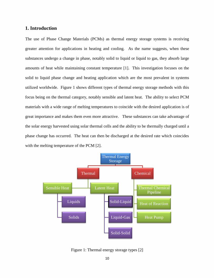
1. Introduction
The use of Phase Change Materials (PCMs) as thermal energy storage systems is receiving
greater attention for applications in heating and cooling. As the name suggests, when these
substances undergo a change in phase, notably solid to liquid or liquid to gas, they absorb large
amounts of heat while maintaining constant temperature [1]. This investigation focuses on the
solid to liquid phase change and heating application which are the most prevalent in systems
utilized worldwide. Figure 1 shows different types of thermal energy storage methods with this
focus being on the thermal category, notably sensible and latent heat. The ability to select PCM
materials with a wide range of melting temperatures to coincide with the desired application is of
great importance and makes them even more attractive. These substances can take advantage of
the solar energy harvested using solar thermal cells and the ability to be thermally charged until a
phase change has occurred. The heat can then be discharged at the desired rate which coincides
with the melting temperature of the PCM [2].
Figure 1: Thermal energy storage types [2]
Thermal Energy Storage
Thermal
Sensible Heat
Liquids
Solids
Latent Heat
Solid-Liquid
Liquid-Gas
Solid-Solid
Chemical
Thermal Chemical Pipeline
Heat of Reaction
Heat Pump
11
A global initiative to push for greener and more efficient methods of storing energy especially
with demand for energy rising has taken shape in PCM related technologies. They inherently
have a high heat of fusion under which melting/solidifying at specific temperatures allows them
the ability to store/release large amounts of heat at usually constant rate [2]. These substances
are called Latent Heat Storage (LHS) systems due to this ability. It is important to note that they
first exhibit the properties of a Sensible Heat Storage (SHS) system whereby their temperature
increases as heat is absorbed. However, once the temperature at which a change in phase is
reached, it then transitions to a LHS entity until a complete change in phase has occurred.
During this LHS phase, the substance absorbs large amounts of heat at an almost constant
temperature. If the temperature falls below the melting point of the PCM, heat is released [2].
There are three major classes of PCMs; organic, inorganic, and eutectic [3]. The advantages and
disadvantages of each class must be taken into account for each application in order to maximize
efficiency and equipment lifetime.
This report focuses on the formulation of a beeswax microemulsion which is chemically stable,
the creation of an experimental apparatus to determine the heat transfer coefficient, and a
comparison between water and the PCM to prove its viability in industry. Techniques in
chemical engineering were used to prepare the beeswax microemulsion and check its stability
for long term use. After a number of failed attempts utilizing pure beeswax, distilled water, and
two chemical surfactants, a successful product was made in bulk to run through the experimental
setup. The setup was made to calculate the heat transfer coefficient of the microemulsion using
an OHS. The system consists of thermocouples, a flow meter, a differential pressure transducer,
a Data Acquisition (DAQ) System, and a power supply as the main tools. Calculations were
done beforehand to size the system correctly and select appropriate materials and fittings to meet
12
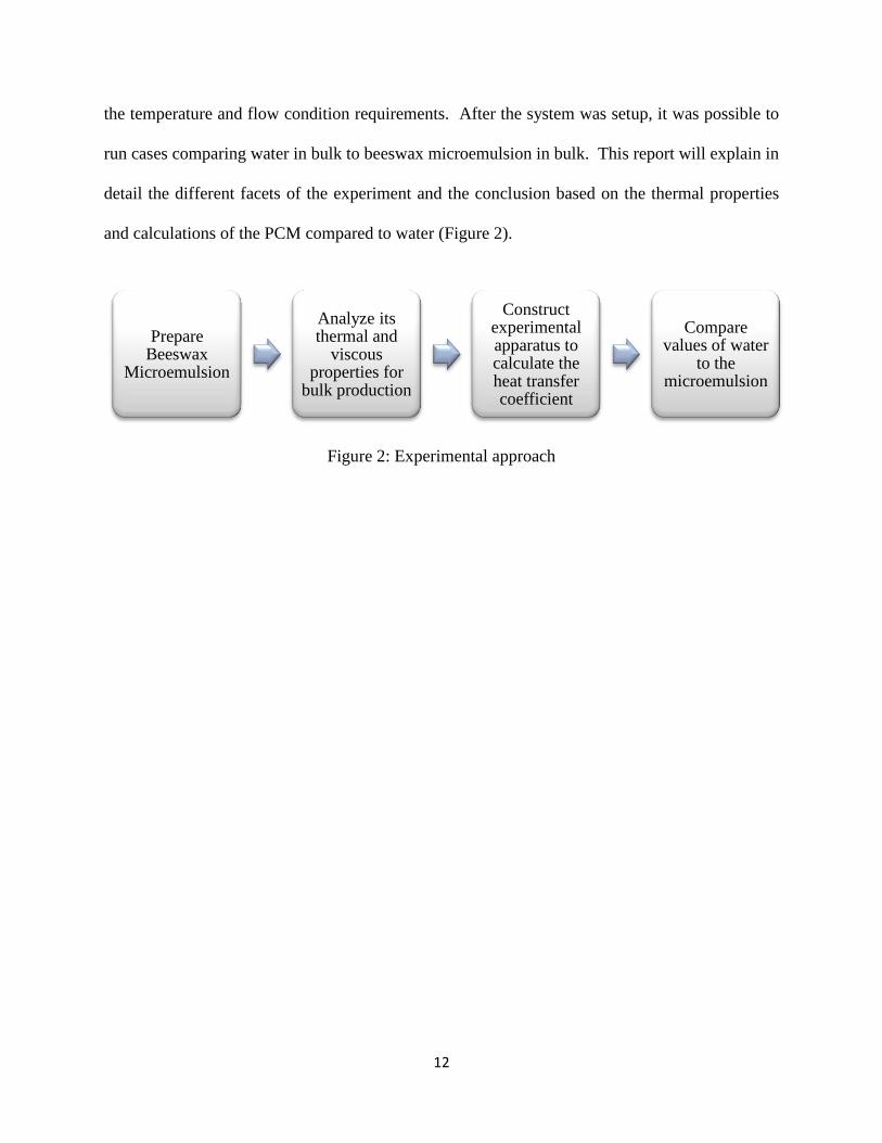
the temperature and flow condition requirements. After the system was setup, it was possible to
run cases comparing water in bulk to beeswax microemulsion in bulk. This report will explain in
detail the different facets of the experiment and the conclusion based on the thermal properties
and calculations of the PCM compared to water (Figure 2).
Figure 2: Experimental approach
Prepare Beeswax
Microemulsion
Analyze its thermal and
viscous properties for
bulk production
Construct experimental apparatus to calculate the heat transfer coefficient
Compare values of water
to the microemulsion
13
2. Classification of PCM materials
As mentioned previously, Phase Change Materials come in different forms, each of which has
advantages and disadvantages depending on the application being investigated. This section
tackles the differences between PCMs and the selection criteria which must be taken into
consideration. PCMs come in a variety of melting temperature ranges with correspondingly
higher heat of fusion compared to existing materials. Choosing the right PCM requires
knowledge about its thermal and viscous properties including the specific heat, thermal
conductivity, and viscosity [3]. These parameters must be within a reasonable range in order to
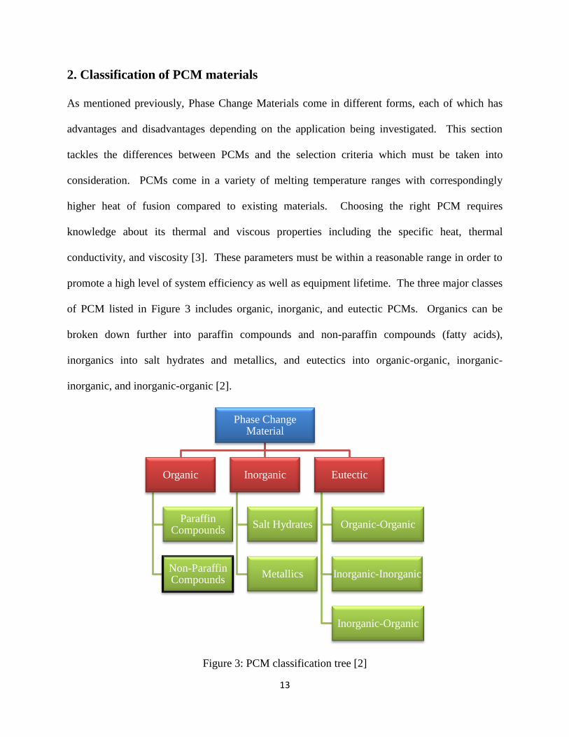
promote a high level of system efficiency as well as equipment lifetime. The three major classes
of PCM listed in Figure 3 includes organic, inorganic, and eutectic PCMs. Organics can be
broken down further into paraffin compounds and non-paraffin compounds (fatty acids),
inorganics into salt hydrates and metallics, and eutectics into organic-organic, inorganic-
inorganic, and inorganic-organic [2].
Figure 3: PCM classification tree [2]
Phase Change Material
Organic
Paraffin Compounds
Non-Paraffin Compounds
Inorganic
Salt Hydrates
Metallics
Eutectic
Organic-Organic
Inorganic-Inorganic
Inorganic-Organic
14
2.1. Organic PCMs
Organic PCMs in paraffin and non-paraffin form are usually the most stable during thermal
cycling without much change in the material's characteristics [4]. Paraffins consists of mixtures
of straight chain n-alkanes CH3-(CH2)-CH3 which store large amounts of latent heat during phase
change. The greater the chain length means the higher the melting point and latent heat of
fusion. Costs are usually an issue for this subclass of PCMs leading only technical grade
materials to be implemented in TES systems. Non-paraffin organic PCMs encompasses the
largest category of possible materials for phase change. This subclass consists of esters, fatty
acids, alcohol's, and glycol's. Fatty acids given by the formula CH3(CH2)2nCOOH have higher
heat of fusion compared to paraffin without super cooling which are both positive qualities.
However, they are in the expensive end of the cost range and show a tendency towards mild
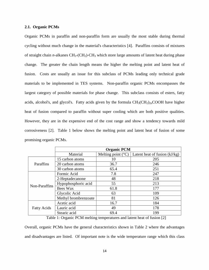
corrosiveness [2]. Table 1 below shows the melting point and latent heat of fusion of some
promising organic PCMs.
Organic PCM
Material Melting point (°C) Latent heat of fusion (kJ/kg)
Paraffins
15 carbon atoms 10 205
20 carbon atoms 36.7 246
30 carbon atoms 65.4 251
Non-Paraffins
Formic Acid 7.8 247
2-Heptadecanone 48 218
Hypophosphoric acid 55 213
Bees Wax 61.8 177
Glycolic Acid 63 109
Methyl brombrenzoate 81 126
Fatty Acids
Acetic acid 16.7 184
Lauric acid 49 178
Stearic acid 69.4 199
Table 1: Organic PCM melting temperatures and latent heat of fusion [2]
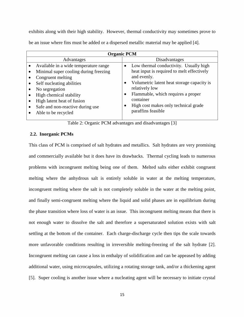
Overall, organic PCMs have the general characteristics shown in Table 2 where the advantages
and disadvantages are listed. Of important note is the wide temperature range which this class
15
exhibits along with their high stability. However, thermal conductivity may sometimes prove to
be an issue where fins must be added or a dispersed metallic material may be applied [4].
Organic PCM
Advantages Disadvantages
Available in a wide temperature range
Minimal super cooling during freezing
Congruent melting
Self nucleating abilities
No segregation
High chemical stability
High latent heat of fusion
Safe and non-reactive during use
Able to be recycled
Low thermal conductivity. Usually high
heat input is required to melt effectively
and evenly.
Volumetric latent heat storage capacity is
relatively low
Flammable, which requires a proper
container
High cost makes only technical grade
paraffins feasible
Table 2: Organic PCM advantages and disadvantages [3]
2.2. Inorganic PCMs
This class of PCM is comprised of salt hydrates and metallics. Salt hydrates are very promising
and commercially available but it does have its drawbacks. Thermal cycling leads to numerous
problems with incongruent melting being one of them. Melted salts either exhibit congruent
melting where the anhydrous salt is entirely soluble in water at the melting temperature,
incongruent melting where the salt is not completely soluble in the water at the melting point,
and finally semi-congruent melting where the liquid and solid phases are in equilibrium during
the phase transition where loss of water is an issue. This incongruent melting means that there is
not enough water to dissolve the salt and therefore a supersaturated solution exists with salt
settling at the bottom of the container. Each charge-discharge cycle then tips the scale towards
more unfavorable conditions resulting in irreversible melting-freezing of the salt hydrate [2].
Incongruent melting can cause a loss in enthalpy of solidification and can be appeased by adding
additional water, using microcapsules, utilizing a rotating storage tank, and/or a thickening agent
[5]. Super cooling is another issue where a nucleating agent will be necessary to initiate crystal
16
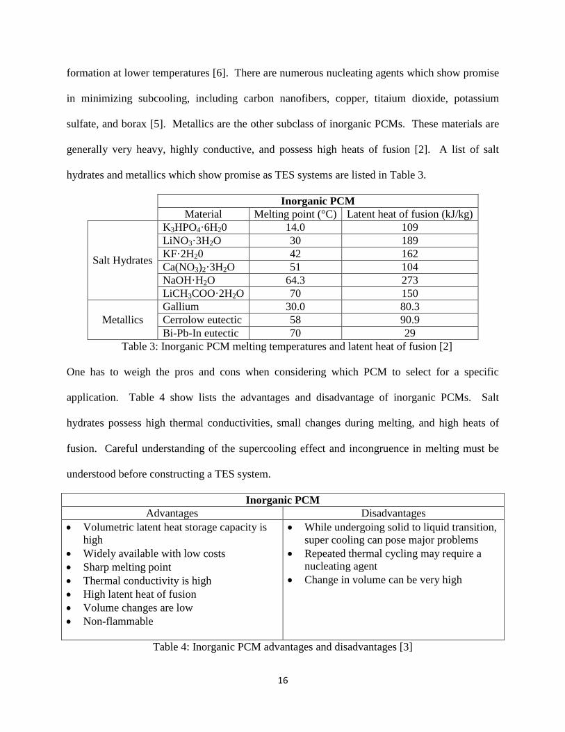
formation at lower temperatures [6]. There are numerous nucleating agents which show promise
in minimizing subcooling, including carbon nanofibers, copper, titaium dioxide, potassium
sulfate, and borax [5]. Metallics are the other subclass of inorganic PCMs. These materials are
generally very heavy, highly conductive, and possess high heats of fusion [2]. A list of salt
hydrates and metallics which show promise as TES systems are listed in Table 3.
Inorganic PCM
Material Melting point (°C) Latent heat of fusion (kJ/kg)
Salt Hydrates
K3HPO4·6H20 14.0 109
LiNO3·3H2O 30 189
KF·2H20 42 162
Ca(NO3)2·3H2O 51 104
NaOH·H2O 64.3 273
LiCH3COO·2H2O 70 150
Metallics
Gallium 30.0 80.3
Cerrolow eutectic 58 90.9
Bi-Pb-In eutectic 70 29
Table 3: Inorganic PCM melting temperatures and latent heat of fusion [2]
One has to weigh the pros and cons when considering which PCM to select for a specific
application. Table 4 show lists the advantages and disadvantage of inorganic PCMs. Salt
hydrates possess high thermal conductivities, small changes during melting, and high heats of
fusion. Careful understanding of the supercooling effect and incongruence in melting must be
understood before constructing a TES system.
Inorganic PCM
Advantages Disadvantages
Volumetric latent heat storage capacity is
high
Widely available with low costs
Sharp melting point
Thermal conductivity is high
High latent heat of fusion
Volume changes are low
Non-flammable
While undergoing solid to liquid transition,
super cooling can pose major problems
Repeated thermal cycling may require a
nucleating agent
Change in volume can be very high
Table 4: Inorganic PCM advantages and disadvantages [3]
17
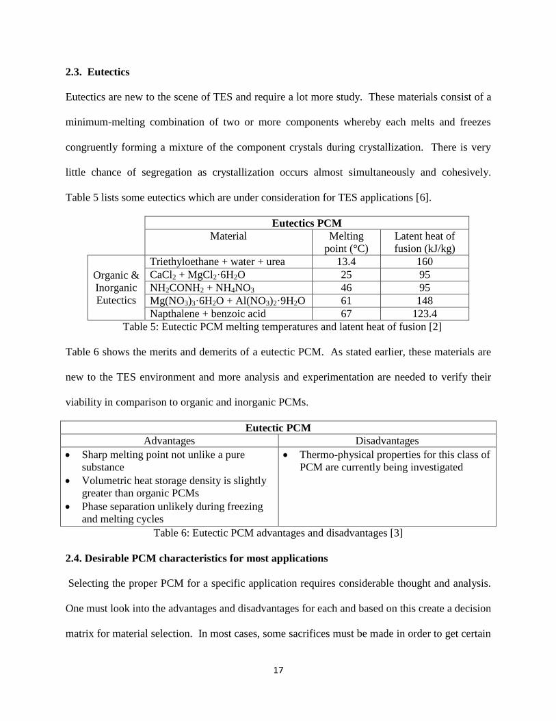
2.3. Eutectics
Eutectics are new to the scene of TES and require a lot more study. These materials consist of a
minimum-melting combination of two or more components whereby each melts and freezes
congruently forming a mixture of the component crystals during crystallization. There is very
little chance of segregation as crystallization occurs almost simultaneously and cohesively.
Table 5 lists some eutectics which are under consideration for TES applications [6].
Eutectics PCM
Material Melting
point (°C)
Latent heat of
fusion (kJ/kg)
Organic &
Inorganic
Eutectics
Triethyloethane + water + urea 13.4 160
CaCl2 + MgCl2·6H2O 25 95
NH2CONH2 + NH4NO3 46 95
Mg(NO3)3·6H2O + Al(NO3)2·9H2O 61 148
Napthalene + benzoic acid 67 123.4
Table 5: Eutectic PCM melting temperatures and latent heat of fusion [2]
Table 6 shows the merits and demerits of a eutectic PCM. As stated earlier, these materials are
new to the TES environment and more analysis and experimentation are needed to verify their
viability in comparison to organic and inorganic PCMs.
Eutectic PCM
Advantages Disadvantages
Sharp melting point not unlike a pure
substance
Volumetric heat storage density is slightly
greater than organic PCMs
Phase separation unlikely during freezing
and melting cycles
Thermo-physical properties for this class of
PCM are currently being investigated
Table 6: Eutectic PCM advantages and disadvantages [3]
2.4. Desirable PCM characteristics for most applications
Selecting the proper PCM for a specific application requires considerable thought and analysis.
One must look into the advantages and disadvantages for each and based on this create a decision
matrix for material selection. In most cases, some sacrifices must be made in order to get certain
18
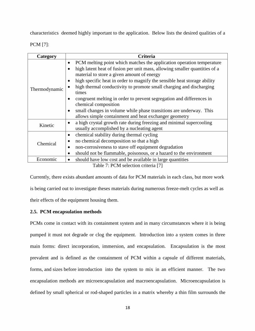
characteristics deemed highly important to the application. Below lists the desired qualities of a
PCM [7]:
Category Criteria
Thermodynamic
PCM melting point which matches the application operation temperature
high latent heat of fusion per unit mass, allowing smaller quantities of a
material to store a given amount of energy
high specific heat in order to magnify the sensible heat storage ability
high thermal conductivity to promote small charging and discharging
times
congruent melting in order to prevent segregation and differences in
chemical composition
small changes in volume while phase transitions are underway. This
allows simple containment and heat exchanger geometry
Kinetic a high crystal growth rate during freezing and minimal supercooling
usually accomplished by a nucleating agent
Chemical
chemical stability during thermal cycling
no chemical decomposition so that a high
non-corrosiveness to stave off equipment degradation
should not be flammable, poisonous, or a hazard to the environment
Economic should have low cost and be available in large quantities
Table 7: PCM selection criteria [7]
Currently, there exists abundant amounts of data for PCM materials in each class, but more work
is being carried out to investigate theses materials during numerous freeze-melt cycles as well as
their effects of the equipment housing them.
2.5. PCM encapsulation methods
PCMs come in contact with its containment system and in many circumstances where it is being
pumped it must not degrade or clog the equipment. Introduction into a system comes in three
main forms: direct incorporation, immersion, and encapsulation. Encapsulation is the most
prevalent and is defined as the containment of PCM within a capsule of different materials,
forms, and sizes before introduction into the system to mix in an efficient manner. The two
encapsulation methods are microencapsulation and macroencapsulation. Microencapsulation is
defined by small spherical or rod-shaped particles in a matrix whereby a thin film surrounds the
19
interface and is compatible with each entity. Macroencapsulation represents the inclusion of
PCM in a form of package such as spheres or tubes which can then operate directly as heat
exchangers [3]. This form can then be easily introduced into building products such as utilizing
capillary mats embedded in PCM plasters as an active system [8]. If the thermal conductivity of
the PCM is not adequate then this method may lead to uneven solidification around the
containment edges thereby preventing uniform and effective heat transfer [3].
Microencapsulation involves very tiny capsules and thus mostly avoids this issue. However, the
higher the concentration of microcapsules the higher the heat storage ability and conversely the
higher the viscosity. Sometimes the concentration reaches a threshold where non-Newtonian
fluid properties come into play and previous analytical models are not applicable [9].
Microencapsulation comes in the form of Phase Change Slurries (PCS) which are binary fluids;
PCM particles in a carrier fluid. Three subgroups includes a shape-stabilized suspension
whereby a PCM suspension is embedded into a support material, microencapsulated suspensions
includes a PCM suspension in water, and PCM/Water-Emulsions includes a dispersion of PCM
droplets in water with the aid of surfactants which will be discussed in the next chapter [10].
20
3. Formulating & Analyzing a Beeswax Microemulsion
This chapter focuses on the formulation of a beeswax microemulsion. Beeswax is an organic
PCM and can be created into an emulsion with the aid of surfactants and water.
3.1. Beeswax background & properties
Pure beeswax was ordered from a California apiary (Hiveharvest) in 1 lb (453.6 g) blocks in
unadulterated form. Beeswax is comprised of esters of fatty acids and long chain alcohols and
fall under the category of organic non-paraffin PCMs. The empirical formula for beeswax is
C15H31COOC30H61. It consists of palmitate, palmitoleate, hydroxypalmitate, and oleate esters of
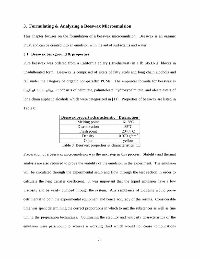
long chain aliphatic alcohols which were categorized in [11]. Properties of beeswax are listed in
Table 8:
Beeswax property/characteristic Description
Melting point 61.8°C
Discoloration 85°C
Flash point 204.4°C
Density 0.970 g/cm3
Color yellow
Table 8: Beeswax properties & characteristics [11]
Preparation of a beeswax microemulsion was the next step in this process. Stability and thermal
analysis are also required to prove the viability of the emulsion in the experiment. The emulsion
will be circulated through the experimental setup and flow through the test section in order to
calculate the heat transfer coefficient. It was important that the liquid emulsion have a low
viscosity and be easily pumped through the system. Any semblance of clogging would prove
detrimental to both the experimental equipment and hence accuracy of the results. Considerable
time was spent determining the correct proportions in which to mix the substances as well as fine
tuning the preparation techniques. Optimizing the stability and viscosity characteristics of the
emulsion were paramount to achieve a working fluid which would not cause complications
21
during the experimental data collection process. A major goal was to formulate a microemulsion
with a large percentage of beeswax by weight in order to increase its latent heat storage abilities.
This can only be done if the viscosity was low enough so that the HTF can be pumped and there
were no significant phase separation phenomena taking place.
Emulsions were macroscopically examined to determine if they can pass the test to become the
bulk HTF to be used in the setup. As mentioned earlier, the main criteria included having a high
percentage of beeswax by weight, possessing low viscosity, and having a high degree of stability
without phase separation. Equipment in the chemistry department were utilized to test the
stability and the specific heat as will be discussed.
3.2. Beeswax microemulsion ingredients and phenomena
An Oil in Water microemulsion needed to be created in order to utilize beeswax as a PCM. A
Phase Change Slurry would be the result of utilizing solid beeswax particles dispersed
throughout the carrier fluid which in this case is water. As is expected, beeswax is not miscible
in water and requires a stabilizing chemical at the interface. This is where surfactants
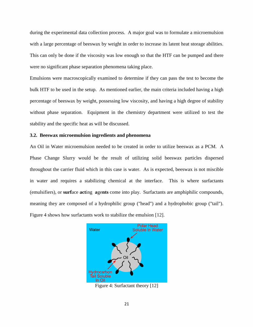
(emulsifiers), or surface acting agents come into play. Surfactants are amphiphilic compounds,
meaning they are composed of a hydrophilic group ("head") and a hydrophobic group ("tail").
Figure 4 shows how surfactants work to stabilize the emulsion [12].
Figure 4: Surfactant theory [12]
22
The hydrocarbon tail orients itself with the "oil" and the polar head orients itself with the
"water." They decrease the energy at the O/W interface required to achieve successful emulsions.
Therefore, to achieve a workable emulsion, the beeswax must first be surrounded by surfactants
before water can be added to encapsulate all the particles [13].
Beeswax acts as the PCM and water as the fluid medium, but surfactants then needed to be
selected. Surfactants are also called emulsifiers and with numerous in the market a system was
developed to choose the appropriate types(s). The HLB system or "Hydrophile-Lipophile
Balance" enables the chemist the ability to assign a number to the ingredient being emulsified
and finding a surfactant or combination of surfactants which will match that number. The
system provides a guideline for choosing emulsifiers which can stabilize the emulsion to a
satisfactory degree which the chemist establishes. In this case, one that adequately encapsulates
the beeswax particles without increasing the viscosity tremendously would be sufficient. HLB
values explains the relative size and strength of the hydrophilic and lipophilic groups in the
emulsifier. Lipophilic surfactants usually have HLB values below 9.0 while hydrophilic types
have HLB values above 11.0. The HLB for cases where multiple emulsifiers are used can be
calculated by the following formula [13]:
Where:
HLB = HLB of both surfactants
% HLB1 = % of surfactant 1
HLB1 = HLB of surfactant 1
% HLB2 = % of surfactant 2
HLB2 = HLB of surfactant 2
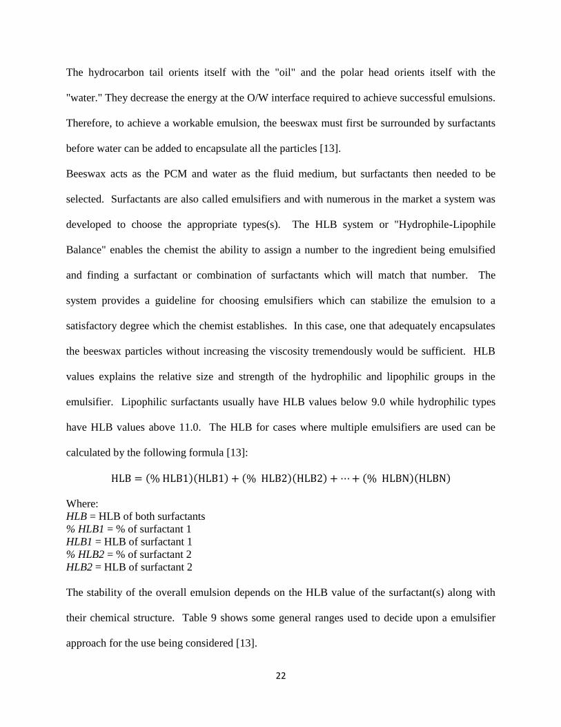
The stability of the overall emulsion depends on the HLB value of the surfactant(s) along with
their chemical structure. Table 9 shows some general ranges used to decide upon a emulsifier
approach for the use being considered [13].
23
HLB Range Use
4-6 W/O emulsifiers
7-9 Wetting agents
8-18 O/W emulsifiers
13-15 Detergents
10-18 Solubilizers
Table 9: HLB ranges and use [13]
If time is limited it has been shown that the following surfactants with stearic acid and stearyl
alcohol derivatives outperform most other types: SPAN 60, TWEEN 60, BRIJ 72, BRIJ 78, and
BRIJ 700. In cases where O/W emulsions are being prepared, higher HLB surfactants lead to
more aqueous solutions which also have lower viscosities. Taking the SPAN 60 (lipophilic) and
TWEEN 60 (hydrophilic) combination which are both stearates and thus have the same chemical
class one can undergo extensive trials to determine the right combination satisfactory for the
application with the HLB 8-18 range in mind [13]. TWEEN 60 (Polyoxyethylene sorbitan
monostearate) and SPAN 60 (Sorbitane Monostearate) were purchased from Sigma Aldrich in
copious amounts to carry out extensive formulations. Increasing the number of surfactants
usually leads to enhanced stability possibly due to the formulation of intermolecular complexes
at the O/W interface and/or development of interfacial films which prevent coalescence [14]. If
time permits and successful results are not achieved, the chemist can try different chemical
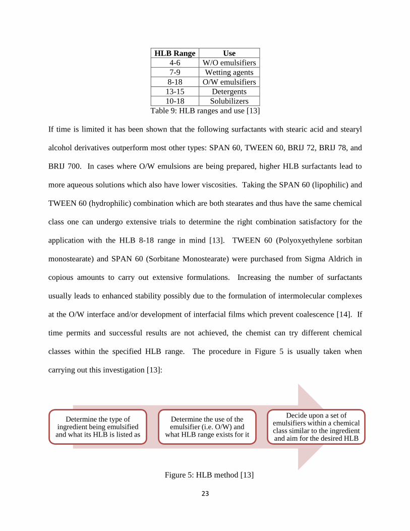
classes within the specified HLB range. The procedure in Figure 5 is usually taken when
carrying out this investigation [13]:
Figure 5: HLB method [13]
Determine the type of ingredient being emulsified and what its HLB is listed as
Determine the use of the emulsifier (i.e. O/W) and
what HLB range exists for it
Decide upon a set of emulsifiers within a chemical class similar to the ingredient and aim for the desired HLB
24
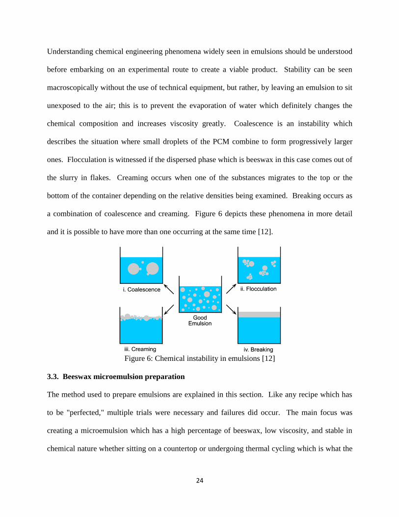
Understanding chemical engineering phenomena widely seen in emulsions should be understood
before embarking on an experimental route to create a viable product. Stability can be seen
macroscopically without the use of technical equipment, but rather, by leaving an emulsion to sit
unexposed to the air; this is to prevent the evaporation of water which definitely changes the
chemical composition and increases viscosity greatly. Coalescence is an instability which
describes the situation where small droplets of the PCM combine to form progressively larger
ones. Flocculation is witnessed if the dispersed phase which is beeswax in this case comes out of
the slurry in flakes. Creaming occurs when one of the substances migrates to the top or the
bottom of the container depending on the relative densities being examined. Breaking occurs as
a combination of coalescence and creaming. Figure 6 depicts these phenomena in more detail
and it is possible to have more than one occurring at the same time [12].
Figure 6: Chemical instability in emulsions [12]
3.3. Beeswax microemulsion preparation
The method used to prepare emulsions are explained in this section. Like any recipe which has
to be "perfected," multiple trials were necessary and failures did occur. The main focus was
creating a microemulsion which has a high percentage of beeswax, low viscosity, and stable in
chemical nature whether sitting on a countertop or undergoing thermal cycling which is what the

25
bulk HTF will undergo. Formulating this beeswax microemulsion required some forethought.
This was a mass and temperature sensitive undertaking which will be explained. First, the
ingredients were prepared in adequate amounts so multiple batches could be made one after
another. The beeswax shown in figure 7 was grated to finer pieces in order to allow more
sensitive weighing (tenths of grams) while also increasing surface area to speed up the melting
process.
Figure 7: Beeswax in bulk and grated form
Figure 8 below shows the ingredients which were necessary to create the microemulsion:
distilled water, TWEEN 60, SPAN 60, and pure beeswax. All the components were liquid or
small enough to be weighed to the tenth of a gram in a mass balance.
Figure 8: Ingredients in microemulsion
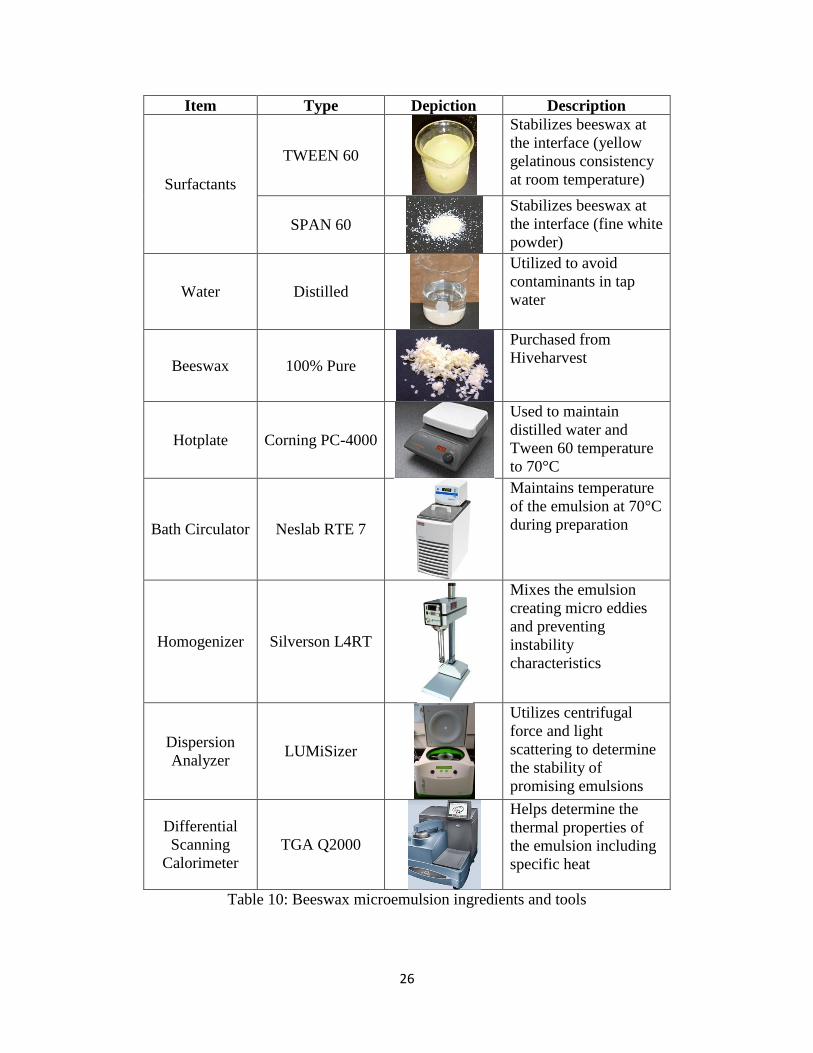
Table 10 shows all the tools necessary to create a proper emulsion using chemical engineering
techniques. The list includes the ingredients, equipment, and tools which were used in the
process.
Water
TWEEN 60
SPAN 60
Beeswax
26
Item Type Depiction Description
Surfactants
TWEEN 60
Stabilizes beeswax at
the interface (yellow
gelatinous consistency
at room temperature)
SPAN 60
Stabilizes beeswax at
the interface (fine white
powder)
Water Distilled
Utilized to avoid
contaminants in tap
water
Beeswax 100% Pure
Purchased from
Hiveharvest
Hotplate Corning PC-4000
Used to maintain
distilled water and
Tween 60 temperature
to 70°C
Bath Circulator Neslab RTE 7
Maintains temperature
of the emulsion at 70°C
during preparation
Homogenizer Silverson L4RT
Mixes the emulsion
creating micro eddies
and preventing
instability
characteristics
Dispersion
Analyzer LUMiSizer
Utilizes centrifugal
force and light
scattering to determine
the stability of
promising emulsions
Differential
Scanning
Calorimeter
TGA Q2000
Helps determine the
thermal properties of
the emulsion including
specific heat
Table 10: Beeswax microemulsion ingredients and tools
27
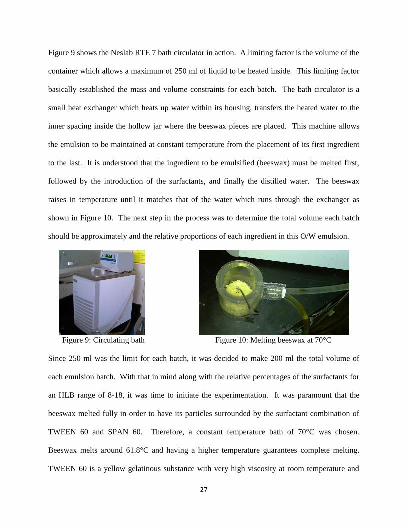
Figure 9 shows the Neslab RTE 7 bath circulator in action. A limiting factor is the volume of the
container which allows a maximum of 250 ml of liquid to be heated inside. This limiting factor
basically established the mass and volume constraints for each batch. The bath circulator is a
small heat exchanger which heats up water within its housing, transfers the heated water to the
inner spacing inside the hollow jar where the beeswax pieces are placed. This machine allows
the emulsion to be maintained at constant temperature from the placement of its first ingredient
to the last. It is understood that the ingredient to be emulsified (beeswax) must be melted first,
followed by the introduction of the surfactants, and finally the distilled water. The beeswax
raises in temperature until it matches that of the water which runs through the exchanger as
shown in Figure 10. The next step in the process was to determine the total volume each batch
should be approximately and the relative proportions of each ingredient in this O/W emulsion.
Figure 9: Circulating bath Figure 10: Melting beeswax at 70°C
Since 250 ml was the limit for each batch, it was decided to make 200 ml the total volume of
each emulsion batch. With that in mind along with the relative percentages of the surfactants for
an HLB range of 8-18, it was time to initiate the experimentation. It was paramount that the
beeswax melted fully in order to have its particles surrounded by the surfactant combination of
TWEEN 60 and SPAN 60. Therefore, a constant temperature bath of 70°C was chosen.
Beeswax melts around 61.8°C and having a higher temperature guarantees complete melting.
TWEEN 60 is a yellow gelatinous substance with very high viscosity at room temperature and
28
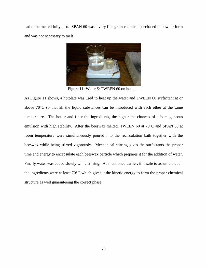
had to be melted fully also. SPAN 60 was a very fine grain chemical purchased in powder form
and was not necessary to melt.
Figure 11: Water & TWEEN 60 on hotplate
As Figure 11 shows, a hotplate was used to heat up the water and TWEEN 60 surfactant at or
above 70°C so that all the liquid substances can be introduced with each other at the same
temperature. The hotter and finer the ingredients, the higher the chances of a homogeneous
emulsion with high stability. After the beeswax melted, TWEEN 60 at 70°C and SPAN 60 at
room temperature were simultaneously poured into the recirculation bath together with the
beeswax while being stirred vigorously. Mechanical stirring gives the surfactants the proper
time and energy to encapsulate each beeswax particle which prepares it for the addition of water.
Finally water was added slowly while stirring. As mentioned earlier, it is safe to assume that all
the ingredients were at least 70°C which gives it the kinetic energy to form the proper chemical
structure as well guaranteeing the correct phase.
29
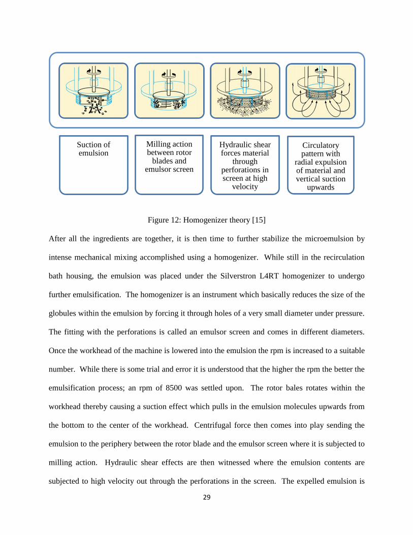
Figure 12: Homogenizer theory [15]
After all the ingredients are together, it is then time to further stabilize the microemulsion by
intense mechanical mixing accomplished using a homogenizer. While still in the recirculation
bath housing, the emulsion was placed under the Silverstron L4RT homogenizer to undergo
further emulsification. The homogenizer is an instrument which basically reduces the size of the
globules within the emulsion by forcing it through holes of a very small diameter under pressure.
The fitting with the perforations is called an emulsor screen and comes in different diameters.
Once the workhead of the machine is lowered into the emulsion the rpm is increased to a suitable
number. While there is some trial and error it is understood that the higher the rpm the better the
emulsification process; an rpm of 8500 was settled upon. The rotor bales rotates within the
workhead thereby causing a suction effect which pulls in the emulsion molecules upwards from
the bottom to the center of the workhead. Centrifugal force then comes into play sending the
emulsion to the periphery between the rotor blade and the emulsor screen where it is subjected to
milling action. Hydraulic shear effects are then witnessed where the emulsion contents are
subjected to high velocity out through the perforations in the screen. The expelled emulsion is
Suction of emulsion
Milling action between rotor
blades and emulsor screen
Hydraulic shear forces material
through perforations in screen at high
velocity
Circulatory pattern with
radial expulsion of material and vertical suction
upwards

30
sent radially to the sides of the mixing vessel as new material is suctioned up in a repeating and
circulatory pattern. This is form of turbulence mixing along with cavitation where small micro
eddies are created which assures homogenization with small globule size in this O/W emulsion.
The process is depicted in Figure 12 which focuses on the workhead area. Figure 13 shows an
tire batch of a few liters being homogenized for introduction into the experimental setup. Froth
can be seen bubbling to the surface during homogenization depicted in Figure 14.
Figure 13: Emulsion being homogenized Figure 14: Froth during homogenization
The general procedure for the entire emulsion preparation process is shown in Figure 15. It was
a tedious process due to the limiting factor of the recirculation bath container but at least the
preparing small batches greatly increases the chances of proper emulsification.
Figure 15: Emulsion preparation process
Weigh: Beeswax,
TWEEN 60, SPAN 60, & Water
Place beeswax into recirculating bath at
70°C and wait for it to melt
Place TWEEN 60 and SPAN 60
simultaneously into the melted beeswax
while stirring
Add distilled water slowly while stirring
While still in recirculating bath,
place homogenizer in emulsion at high rpm
for atleast 15 min
Pour emulsion into a closed container and begin another batch
31
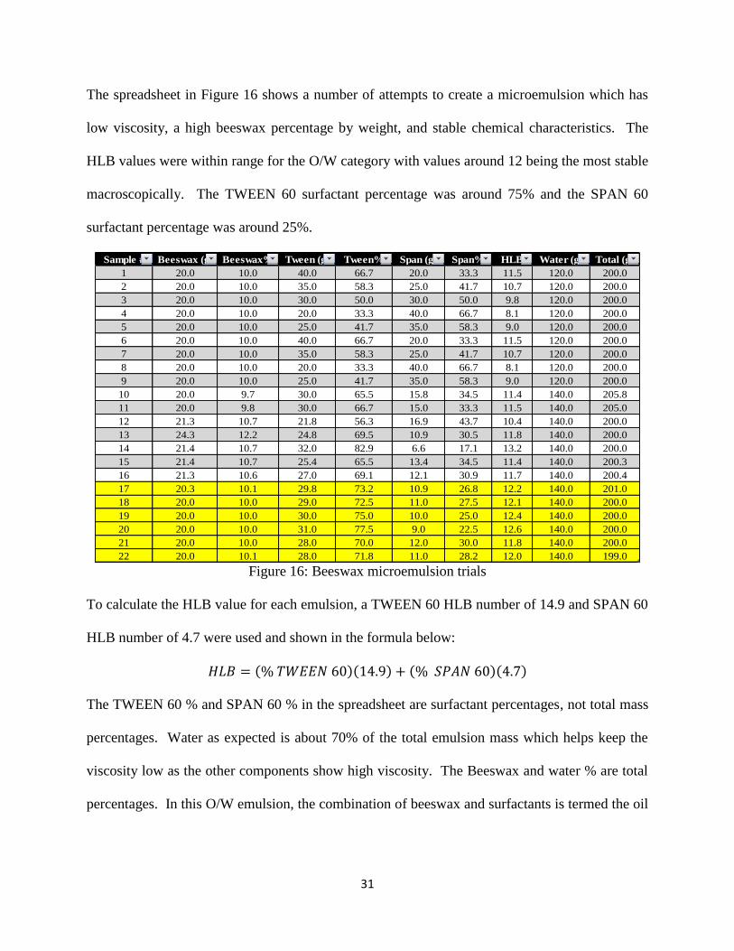
The spreadsheet in Figure 16 shows a number of attempts to create a microemulsion which has
low viscosity, a high beeswax percentage by weight, and stable chemical characteristics. The
HLB values were within range for the O/W category with values around 12 being the most stable
macroscopically. The TWEEN 60 surfactant percentage was around 75% and the SPAN 60
surfactant percentage was around 25%.
Sample # Beeswax (g) Beeswax% Tween (g) Tween% Span (g) Span% HLB Water (g) Total (g)
1 20.0 10.0 40.0 66.7 20.0 33.3 11.5 120.0 200.0
2 20.0 10.0 35.0 58.3 25.0 41.7 10.7 120.0 200.0
3 20.0 10.0 30.0 50.0 30.0 50.0 9.8 120.0 200.0
4 20.0 10.0 20.0 33.3 40.0 66.7 8.1 120.0 200.0
5 20.0 10.0 25.0 41.7 35.0 58.3 9.0 120.0 200.0
6 20.0 10.0 40.0 66.7 20.0 33.3 11.5 120.0 200.0
7 20.0 10.0 35.0 58.3 25.0 41.7 10.7 120.0 200.0
8 20.0 10.0 20.0 33.3 40.0 66.7 8.1 120.0 200.0
9 20.0 10.0 25.0 41.7 35.0 58.3 9.0 120.0 200.0
10 20.0 9.7 30.0 65.5 15.8 34.5 11.4 140.0 205.8
11 20.0 9.8 30.0 66.7 15.0 33.3 11.5 140.0 205.0
12 21.3 10.7 21.8 56.3 16.9 43.7 10.4 140.0 200.0
13 24.3 12.2 24.8 69.5 10.9 30.5 11.8 140.0 200.0
14 21.4 10.7 32.0 82.9 6.6 17.1 13.2 140.0 200.0
15 21.4 10.7 25.4 65.5 13.4 34.5 11.4 140.0 200.3
16 21.3 10.6 27.0 69.1 12.1 30.9 11.7 140.0 200.4
17 20.3 10.1 29.8 73.2 10.9 26.8 12.2 140.0 201.0
18 20.0 10.0 29.0 72.5 11.0 27.5 12.1 140.0 200.0
19 20.0 10.0 30.0 75.0 10.0 25.0 12.4 140.0 200.0
20 20.0 10.0 31.0 77.5 9.0 22.5 12.6 140.0 200.0
21 20.0 10.0 28.0 70.0 12.0 30.0 11.8 140.0 200.0
22 20.0 10.1 28.0 71.8 11.0 28.2 12.0 140.0 199.0
Figure 16: Beeswax microemulsion trials
To calculate the HLB value for each emulsion, a TWEEN 60 HLB number of 14.9 and SPAN 60
HLB number of 4.7 were used and shown in the formula below:
The TWEEN 60 % and SPAN 60 % in the spreadsheet are surfactant percentages, not total mass
percentages. Water as expected is about 70% of the total emulsion mass which helps keep the
viscosity low as the other components show high viscosity. The Beeswax and water % are total
percentages. In this O/W emulsion, the combination of beeswax and surfactants is termed the oil
32
(O) while the distilled water is the (W). From the trials carried it is appears that the O/W
combination of 30%/70% were the most successful (yellow).
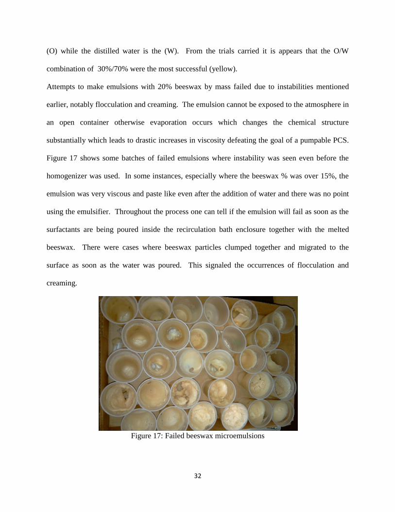
Attempts to make emulsions with 20% beeswax by mass failed due to instabilities mentioned
earlier, notably flocculation and creaming. The emulsion cannot be exposed to the atmosphere in
an open container otherwise evaporation occurs which changes the chemical structure
substantially which leads to drastic increases in viscosity defeating the goal of a pumpable PCS.
Figure 17 shows some batches of failed emulsions where instability was seen even before the
homogenizer was used. In some instances, especially where the beeswax % was over 15%, the
emulsion was very viscous and paste like even after the addition of water and there was no point
using the emulsifier. Throughout the process one can tell if the emulsion will fail as soon as the
surfactants are being poured inside the recirculation bath enclosure together with the melted
beeswax. There were cases where beeswax particles clumped together and migrated to the
surface as soon as the water was poured. This signaled the occurrences of flocculation and
creaming.
Figure 17: Failed beeswax microemulsions

33
Magnification Appearance Scale Length
10X
200µm
20X
200µm
50X
50µm
100X
20µm
Table 11: Beeswax microemulsion under microscope
34
Table 11 shows the winning emulsion under a microscope under various magnifications. The
next section will discuss the stability analysis of the chosen emulsion which basically looked at
the top performing emulsions from the trials. The trial which performed best in the stability
analysis was produced in bulk to be run in the system. Since this is a microemulsion it is
expected to see the particles down to the micron level. The appearance at magnification 10X has
a bubble seen in the top left and is not important. Further magnifications show the homogeneity
in the emulsion chemical structure. The complexes are uniformly dispersed and microscopic in
size which bodes well in the stability category. Given enough time and no agitation, these
microemulsions will revert back to their individual layers and segregate out for the most part.
Mechanical work or heat application may be necessary to delay phase separation. In this
investigated, the fluid will be continually undergo motion and thermal cycling which helps
maintain homogeneity.
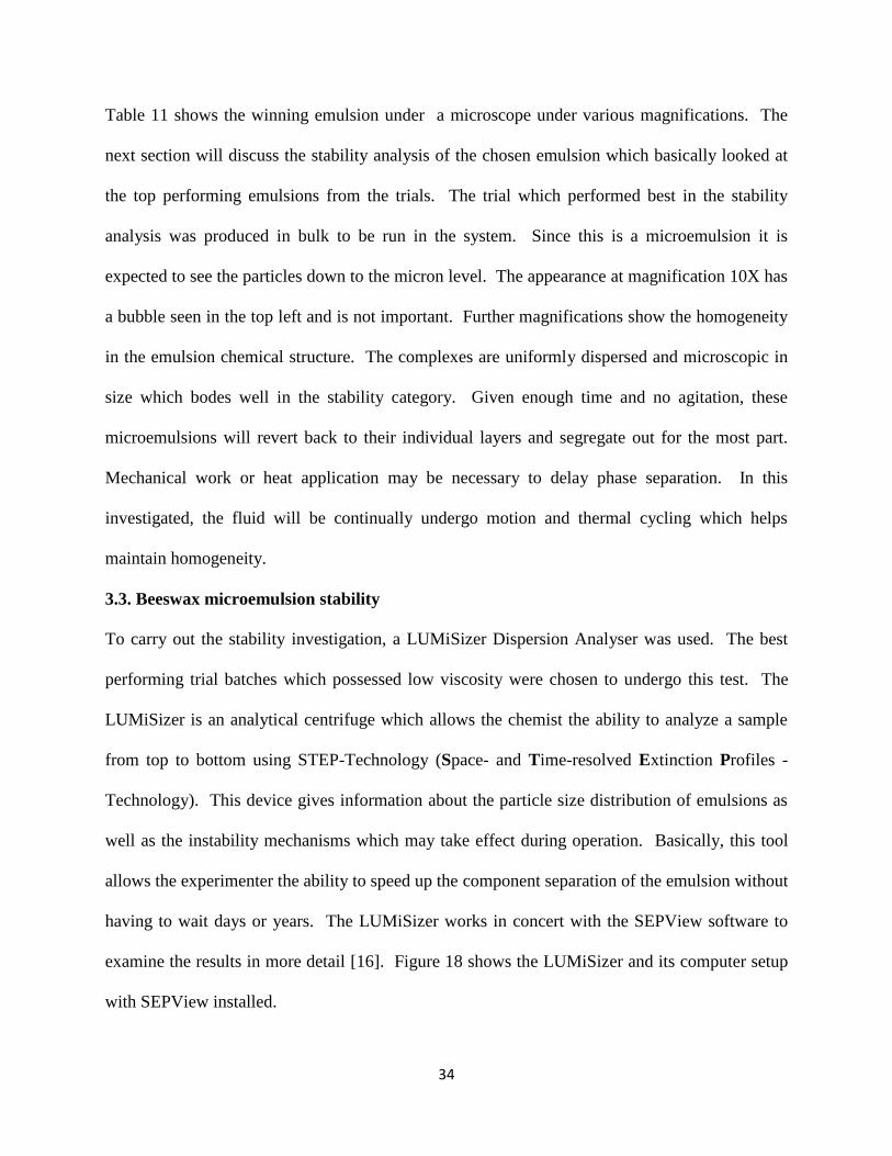
3.3. Beeswax microemulsion stability
To carry out the stability investigation, a LUMiSizer Dispersion Analyser was used. The best
performing trial batches which possessed low viscosity were chosen to undergo this test. The
LUMiSizer is an analytical centrifuge which allows the chemist the ability to analyze a sample
from top to bottom using STEP-Technology (Space- and Time-resolved Extinction Profiles -
Technology). This device gives information about the particle size distribution of emulsions as
well as the instability mechanisms which may take effect during operation. Basically, this tool
allows the experimenter the ability to speed up the component separation of the emulsion without
having to wait days or years. The LUMiSizer works in concert with the SEPView software to
examine the results in more detail [16]. Figure 18 shows the LUMiSizer and its computer setup
with SEPView installed.
35
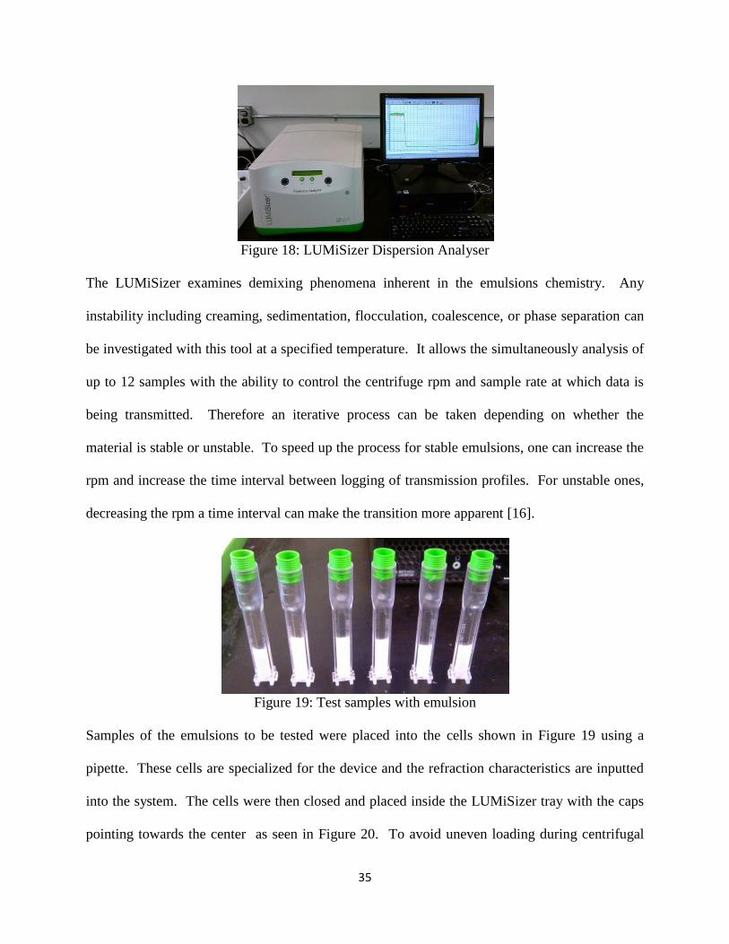
Figure 18: LUMiSizer Dispersion Analyser
The LUMiSizer examines demixing phenomena inherent in the emulsions chemistry. Any
instability including creaming, sedimentation, flocculation, coalescence, or phase separation can
be investigated with this tool at a specified temperature. It allows the simultaneously analysis of
up to 12 samples with the ability to control the centrifuge rpm and sample rate at which data is
being transmitted. Therefore an iterative process can be taken depending on whether the
material is stable or unstable. To speed up the process for stable emulsions, one can increase the
rpm and increase the time interval between logging of transmission profiles. For unstable ones,
decreasing the rpm a time interval can make the transition more apparent [16].
Figure 19: Test samples with emulsion
Samples of the emulsions to be tested were placed into the cells shown in Figure 19 using a
pipette. These cells are specialized for the device and the refraction characteristics are inputted
into the system. The cells were then closed and placed inside the LUMiSizer tray with the caps
pointing towards the center as seen in Figure 20. To avoid uneven loading during centrifugal
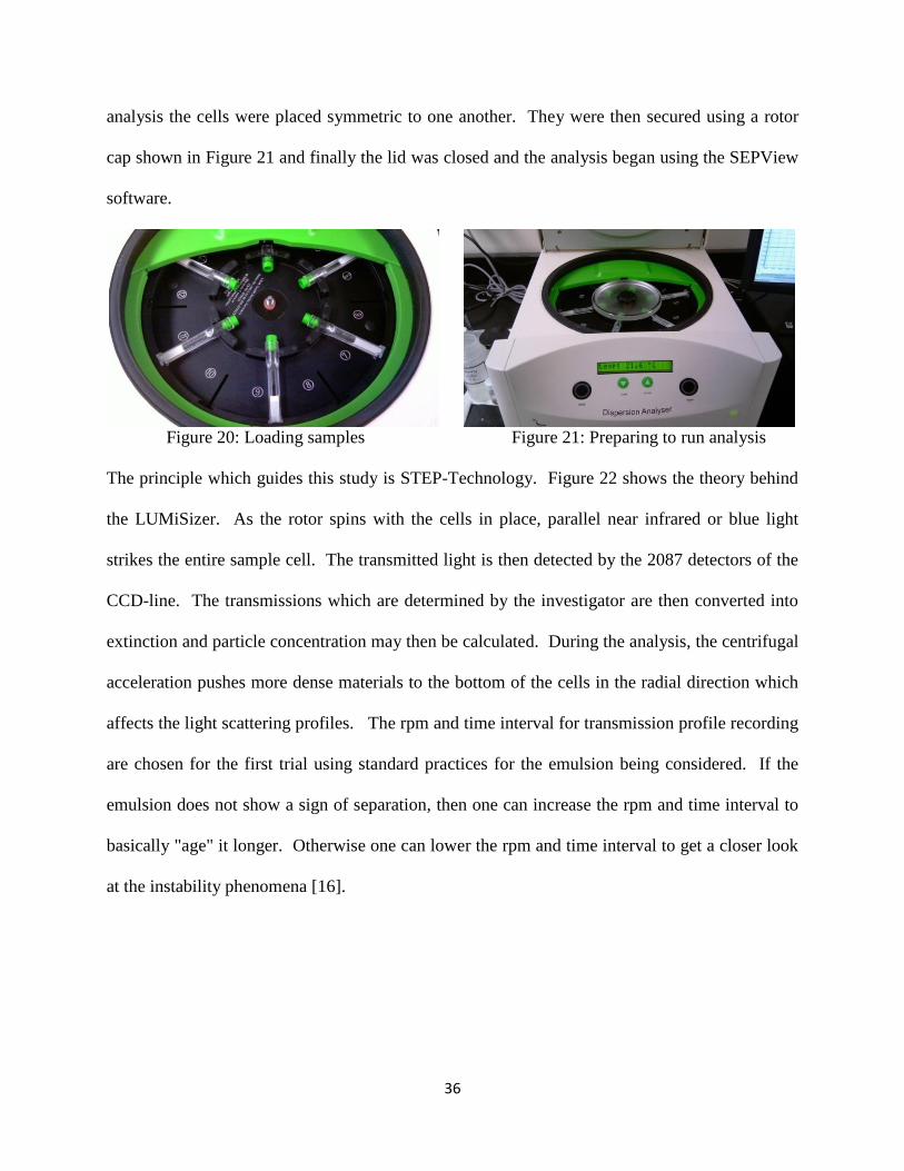
36
analysis the cells were placed symmetric to one another. They were then secured using a rotor
cap shown in Figure 21 and finally the lid was closed and the analysis began using the SEPView
software.
Figure 20: Loading samples Figure 21: Preparing to run analysis
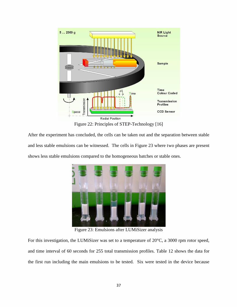
The principle which guides this study is STEP-Technology. Figure 22 shows the theory behind
the LUMiSizer. As the rotor spins with the cells in place, parallel near infrared or blue light
strikes the entire sample cell. The transmitted light is then detected by the 2087 detectors of the
CCD-line. The transmissions which are determined by the investigator are then converted into
extinction and particle concentration may then be calculated. During the analysis, the centrifugal
acceleration pushes more dense materials to the bottom of the cells in the radial direction which
affects the light scattering profiles. The rpm and time interval for transmission profile recording
are chosen for the first trial using standard practices for the emulsion being considered. If the
emulsion does not show a sign of separation, then one can increase the rpm and time interval to
basically "age" it longer. Otherwise one can lower the rpm and time interval to get a closer look
at the instability phenomena [16].
37
Figure 22: Principles of STEP-Technology [16]
After the experiment has concluded, the cells can be taken out and the separation between stable
and less stable emulsions can be witnessed. The cells in Figure 23 where two phases are present
shows less stable emulsions compared to the homogeneous batches or stable ones.
Figure 23: Emulsions after LUMiSizer analysis
For this investigation, the LUMiSizer was set to a temperature of 20°C, a 3000 rpm rotor speed,
and time interval of 60 seconds for 255 total transmission profiles. Table 12 shows the data for
the first run including the main emulsions to be tested. Six were tested in the device because
38
they possessed macroscopic stability and low viscosity. They were loaded symmetrically into
the LUMiSizer and SEPView was programmed to run.
RUN 1: T=20°C, RPM=3000, t=60s
Sample Beeswax % TWEEN 60 % SPAN 60 % Oil % Water %
17 10.1 14.83 5.42 30% 70
18 10.0 14.50 5.50 30% 70
19 10.0 15.00 5.00 30% 70
20 10.0 15.50 4.50 30% 70
21 10.0 14.00 6.00 30% 70
22 10.0 14.07 5.52 30% 70
Table 12: Samples tested in LUMiSizer (RUN 1)
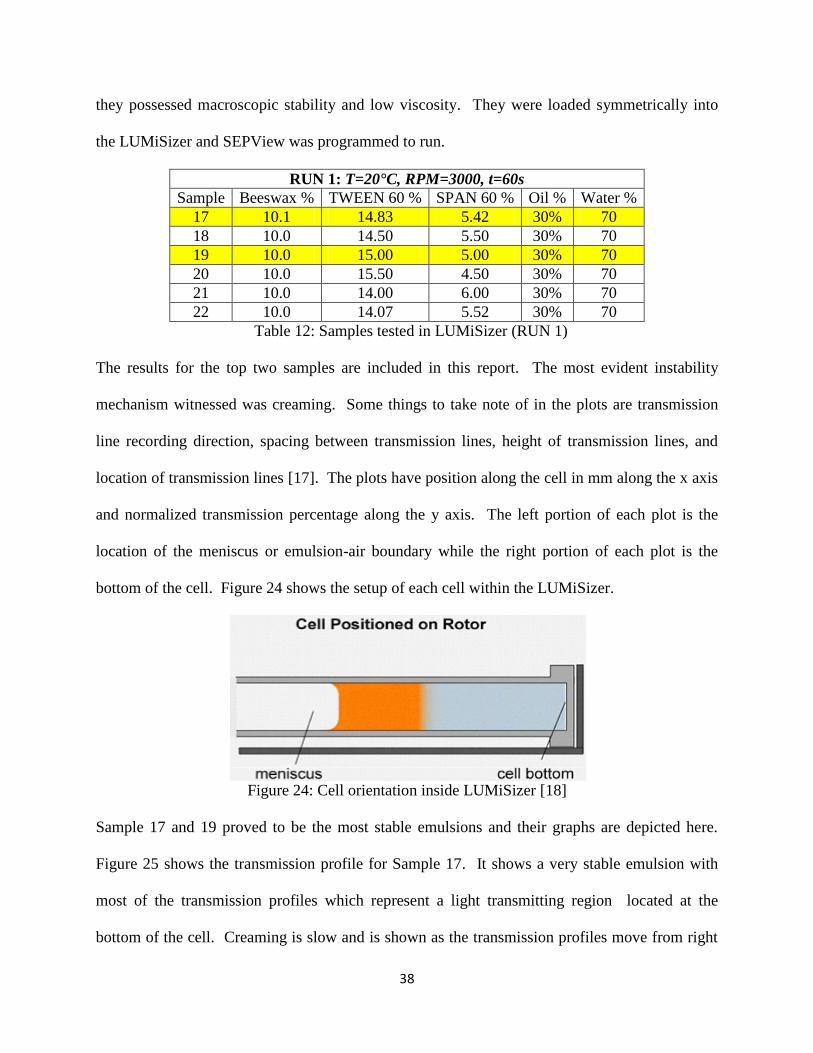
The results for the top two samples are included in this report. The most evident instability
mechanism witnessed was creaming. Some things to take note of in the plots are transmission
line recording direction, spacing between transmission lines, height of transmission lines, and
location of transmission lines [17]. The plots have position along the cell in mm along the x axis
and normalized transmission percentage along the y axis. The left portion of each plot is the
location of the meniscus or emulsion-air boundary while the right portion of each plot is the
bottom of the cell. Figure 24 shows the setup of each cell within the LUMiSizer.
Figure 24: Cell orientation inside LUMiSizer [18]
Sample 17 and 19 proved to be the most stable emulsions and their graphs are depicted here.
Figure 25 shows the transmission profile for Sample 17. It shows a very stable emulsion with
most of the transmission profiles which represent a light transmitting region located at the
bottom of the cell. Creaming is slow and is shown as the transmission profiles move from right

39
to left [19]. The spacing between the profiles is also miniscule dictating a slow process. The
normalized transmission percentage is around 55% for the small region where light is being
transmitted.
Figure 25: Transmission profiles for Sample 17 in RUN 1
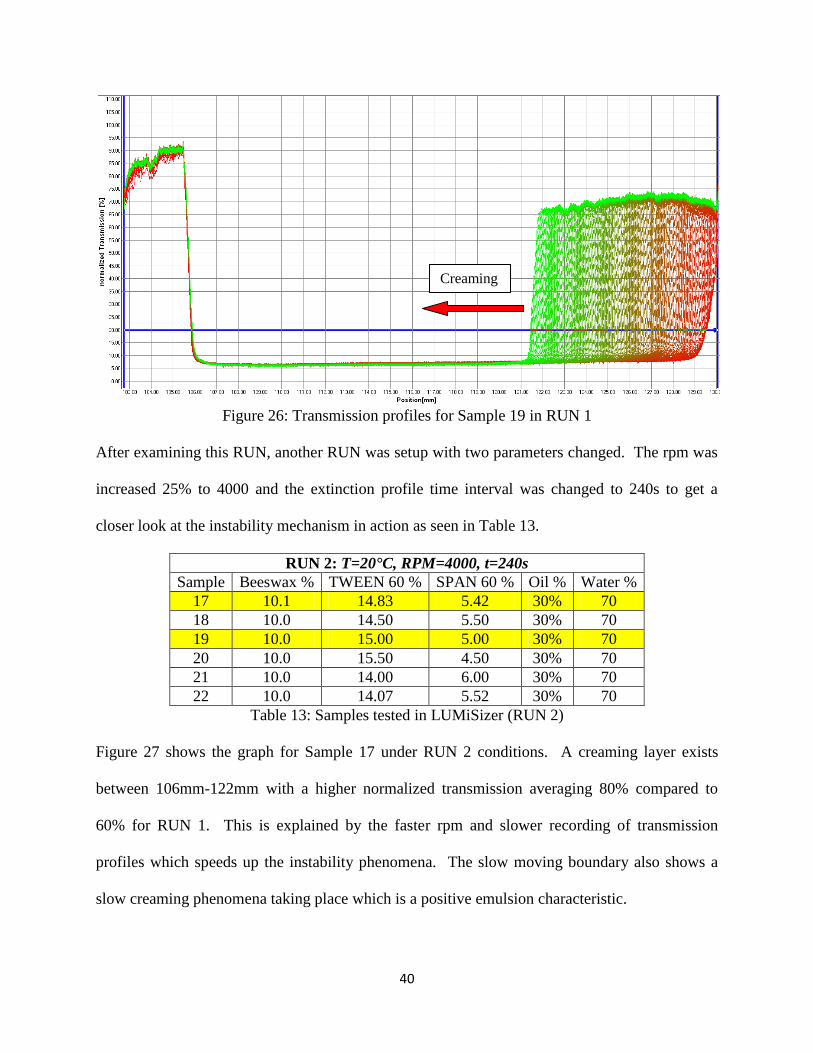
The graph for Sample 19 is shown in Figure 26. The transmission profiles are more spread out
and the light transmitting region is larger than that of Sample 17. Sample 19 has slightly more
TWEEN 60 and slightly less SPAN 60 with beeswax and water percentages basically the same.
The small change in chemistry led to a more pronounced transmission profile. Creaming unlike
other phenomena can be reversed with some mechanical work such as continued homogenizing
or mixing. After centrifugation, a creaming layer exists between 106mm-121mm in the top of
the cell. There is a steady movement between transmission profiles of the liquid-solid boundary
from right to left establishing the creaming layer. With increased centrifugation there is also
increased transmission of light with a normalized transmission about 65% [17]. Zones of well
mixed dispersions scatter the light leading to low transmissions while increased transparency
enables more light to reach the CCD-line signaling high transmissions [20].
Creaming
liquid
-air
boun
dar
y
Meniscus
40
Figure 26: Transmission profiles for Sample 19 in RUN 1
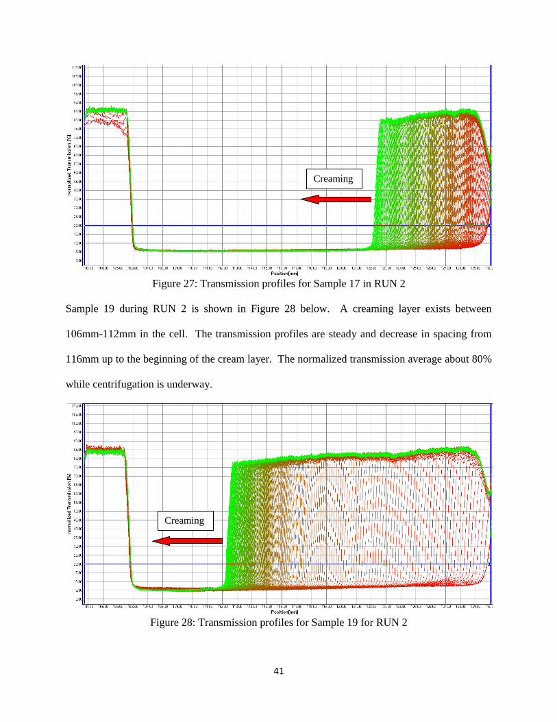
After examining this RUN, another RUN was setup with two parameters changed. The rpm was
increased 25% to 4000 and the extinction profile time interval was changed to 240s to get a
closer look at the instability mechanism in action as seen in Table 13.
RUN 2: T=20°C, RPM=4000, t=240s
Sample Beeswax % TWEEN 60 % SPAN 60 % Oil % Water %
17 10.1 14.83 5.42 30% 70
18 10.0 14.50 5.50 30% 70
19 10.0 15.00 5.00 30% 70
20 10.0 15.50 4.50 30% 70
21 10.0 14.00 6.00 30% 70
22 10.0 14.07 5.52 30% 70
Table 13: Samples tested in LUMiSizer (RUN 2)
Figure 27 shows the graph for Sample 17 under RUN 2 conditions. A creaming layer exists
between 106mm-122mm with a higher normalized transmission averaging 80% compared to
60% for RUN 1. This is explained by the faster rpm and slower recording of transmission
profiles which speeds up the instability phenomena. The slow moving boundary also shows a
slow creaming phenomena taking place which is a positive emulsion characteristic.
Creaming
41
Figure 27: Transmission profiles for Sample 17 in RUN 2
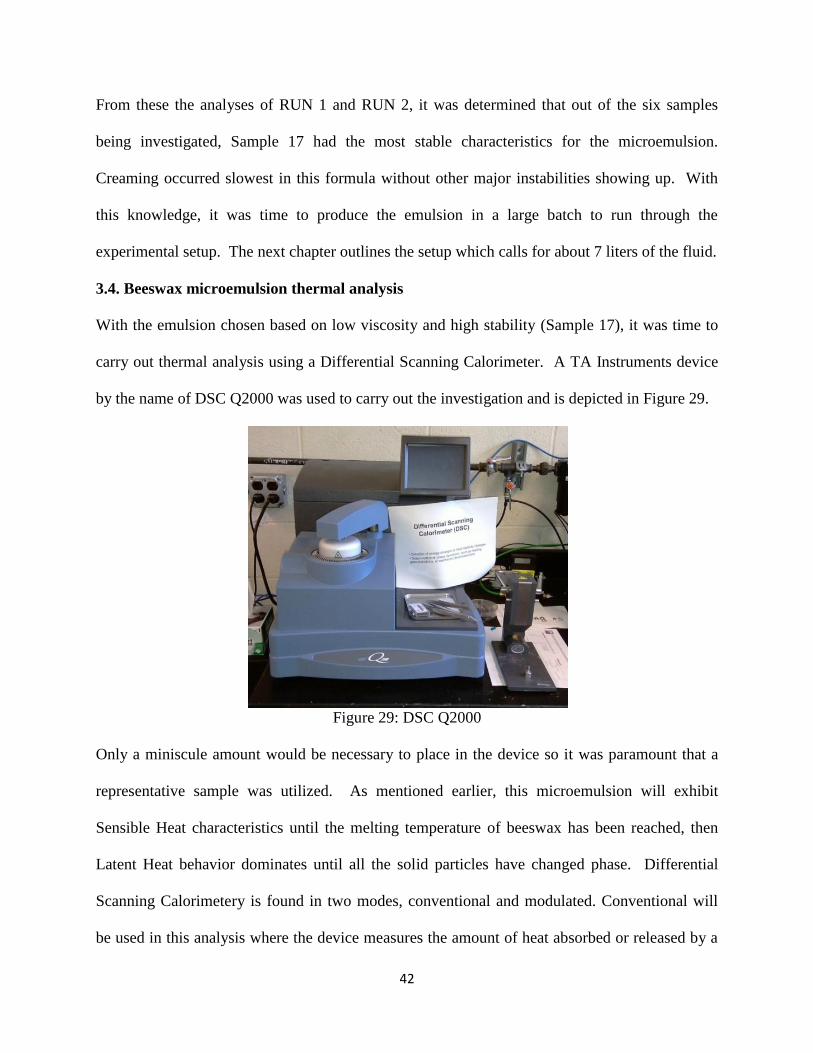
Sample 19 during RUN 2 is shown in Figure 28 below. A creaming layer exists between
106mm-112mm in the cell. The transmission profiles are steady and decrease in spacing from
116mm up to the beginning of the cream layer. The normalized transmission average about 80%
while centrifugation is underway.
Figure 28: Transmission profiles for Sample 19 for RUN 2
Creaming
Creaming
42
From these the analyses of RUN 1 and RUN 2, it was determined that out of the six samples
being investigated, Sample 17 had the most stable characteristics for the microemulsion.
Creaming occurred slowest in this formula without other major instabilities showing up. With
this knowledge, it was time to produce the emulsion in a large batch to run through the
experimental setup. The next chapter outlines the setup which calls for about 7 liters of the fluid.
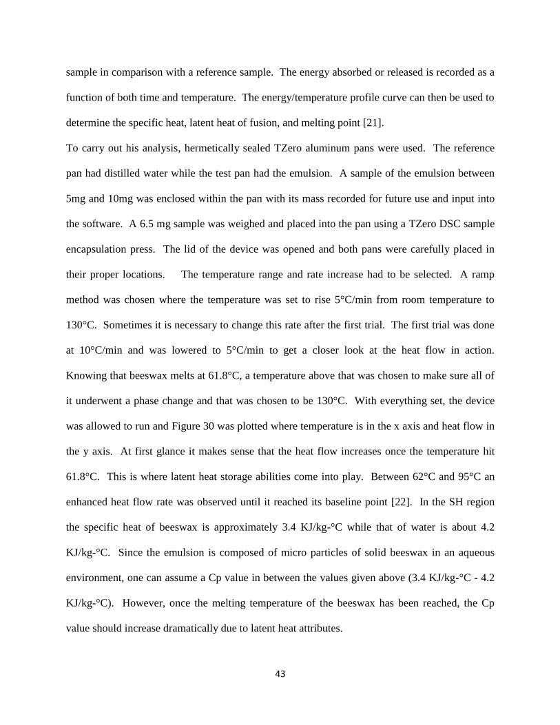
3.4. Beeswax microemulsion thermal analysis
With the emulsion chosen based on low viscosity and high stability (Sample 17), it was time to
carry out thermal analysis using a Differential Scanning Calorimeter. A TA Instruments device
by the name of DSC Q2000 was used to carry out the investigation and is depicted in Figure 29.
Figure 29: DSC Q2000
Only a miniscule amount would be necessary to place in the device so it was paramount that a
representative sample was utilized. As mentioned earlier, this microemulsion will exhibit
Sensible Heat characteristics until the melting temperature of beeswax has been reached, then
Latent Heat behavior dominates until all the solid particles have changed phase. Differential
Scanning Calorimetery is found in two modes, conventional and modulated. Conventional will
be used in this analysis where the device measures the amount of heat absorbed or released by a
43
sample in comparison with a reference sample. The energy absorbed or released is recorded as a
function of both time and temperature. The energy/temperature profile curve can then be used to
determine the specific heat, latent heat of fusion, and melting point [21].
To carry out his analysis, hermetically sealed TZero aluminum pans were used. The reference
pan had distilled water while the test pan had the emulsion. A sample of the emulsion between
5mg and 10mg was enclosed within the pan with its mass recorded for future use and input into
the software. A 6.5 mg sample was weighed and placed into the pan using a TZero DSC sample
encapsulation press. The lid of the device was opened and both pans were carefully placed in
their proper locations. The temperature range and rate increase had to be selected. A ramp
method was chosen where the temperature was set to rise 5°C/min from room temperature to
130°C. Sometimes it is necessary to change this rate after the first trial. The first trial was done
at 10°C/min and was lowered to 5°C/min to get a closer look at the heat flow in action.
Knowing that beeswax melts at 61.8°C, a temperature above that was chosen to make sure all of
it underwent a phase change and that was chosen to be 130°C. With everything set, the device
was allowed to run and Figure 30 was plotted where temperature is in the x axis and heat flow in
the y axis. At first glance it makes sense that the heat flow increases once the temperature hit
61.8°C. This is where latent heat storage abilities come into play. Between 62°C and 95°C an
enhanced heat flow rate was observed until it reached its baseline point [22]. In the SH region
the specific heat of beeswax is approximately 3.4 KJ/kg-°C while that of water is about 4.2
KJ/kg-°C. Since the emulsion is composed of micro particles of solid beeswax in an aqueous
environment, one can assume a Cp value in between the values given above (3.4 KJ/kg-°C - 4.2
KJ/kg-°C). However, once the melting temperature of the beeswax has been reached, the Cp
value should increase dramatically due to latent heat attributes.
44
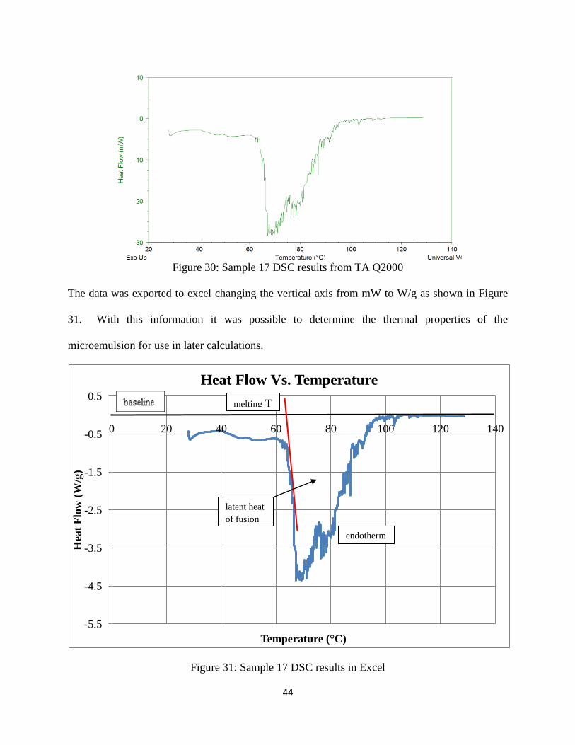
Figure 30: Sample 17 DSC results from TA Q2000
The data was exported to excel changing the vertical axis from mW to W/g as shown in Figure
31. With this information it was possible to determine the thermal properties of the
microemulsion for use in later calculations.
Figure 31: Sample 17 DSC results in Excel
-5.5
-4.5
-3.5
-2.5
-1.5
-0.5
0.5
0 20 40 60 80 100 120 140
Hea
t F
low
(W
/g)
Temperature (°C)
Heat Flow Vs. Temperature
melting T
latent heat
of fusion
endotherm
45
Figure 31 depicts an endotherm curve in blue and baseline in black. The melting temperature
can be checked by finding the point at which the tangent of the maximum rising slope intercepts
the baseline, shown by the red line in Figure 31 with a temperature of about 62°C . The latent
heat of fusion can be calculated by finding the area enclosed between the endotherm curve and
the baseline [22]. The data in Excel was used to determine this value which gave a latent heat of
fusion of 185.88 KJ/kg. This value is representative of 10% beeswax surrounded by stabilizing
surfactants in an aqueous water solution.
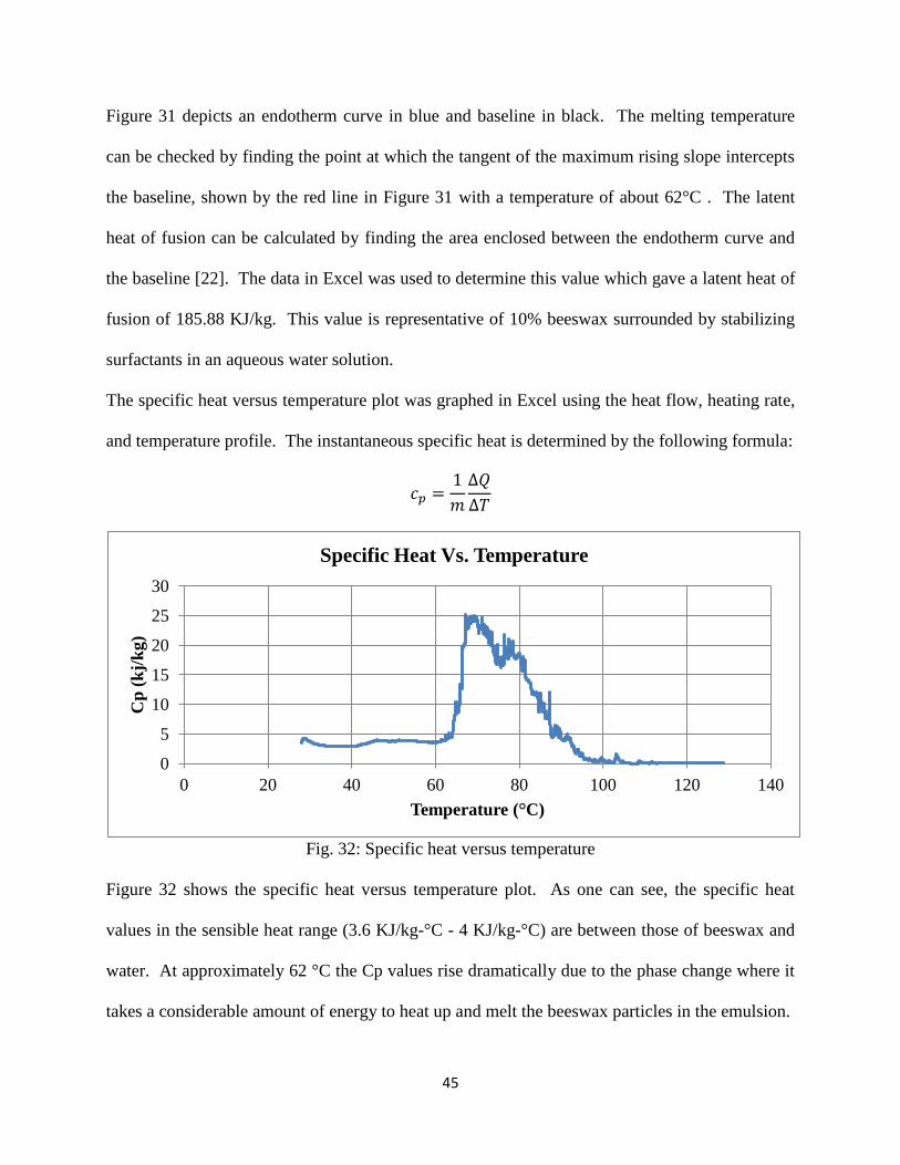
The specific heat versus temperature plot was graphed in Excel using the heat flow, heating rate,
and temperature profile. The instantaneous specific heat is determined by the following formula:
Fig. 32: Specific heat versus temperature
Figure 32 shows the specific heat versus temperature plot. As one can see, the specific heat
values in the sensible heat range (3.6 KJ/kg-°C - 4 KJ/kg-°C) are between those of beeswax and
water. At approximately 62 °C the Cp values rise dramatically due to the phase change where it
takes a considerable amount of energy to heat up and melt the beeswax particles in the emulsion.
0
5
10
15
20
25
30
0 20 40 60 80 100 120 140
Cp
(k
j/k
g)
Temperature (°C)
Specific Heat Vs. Temperature
46
4. Constructing the Experimental Setup
The experimental setup was necessary to determine the heat transfer coefficient of the beeswax
microemulsion. The setup was validated by first running water through the system. Design and
construction of the experimental setup was done together with the emulsion formulation. The
viscosity of the emulsion had to be low and the chemical nature of it had to be non-corrosive to
prevent tubing and pipe degradation. The main focus of the apparatus was the test section
region which would undergo ohmic heating by means of a power supply. Since this was a
temperature sensitive experiment, it was essential that all components coming in contact with the
HTF have operating temperatures above 70 °C. Proper selection of each device was necessary to
obtain results in an efficient manner. As in any experiment, troubleshooting was extensive as
problems arose throughout the data collection process.
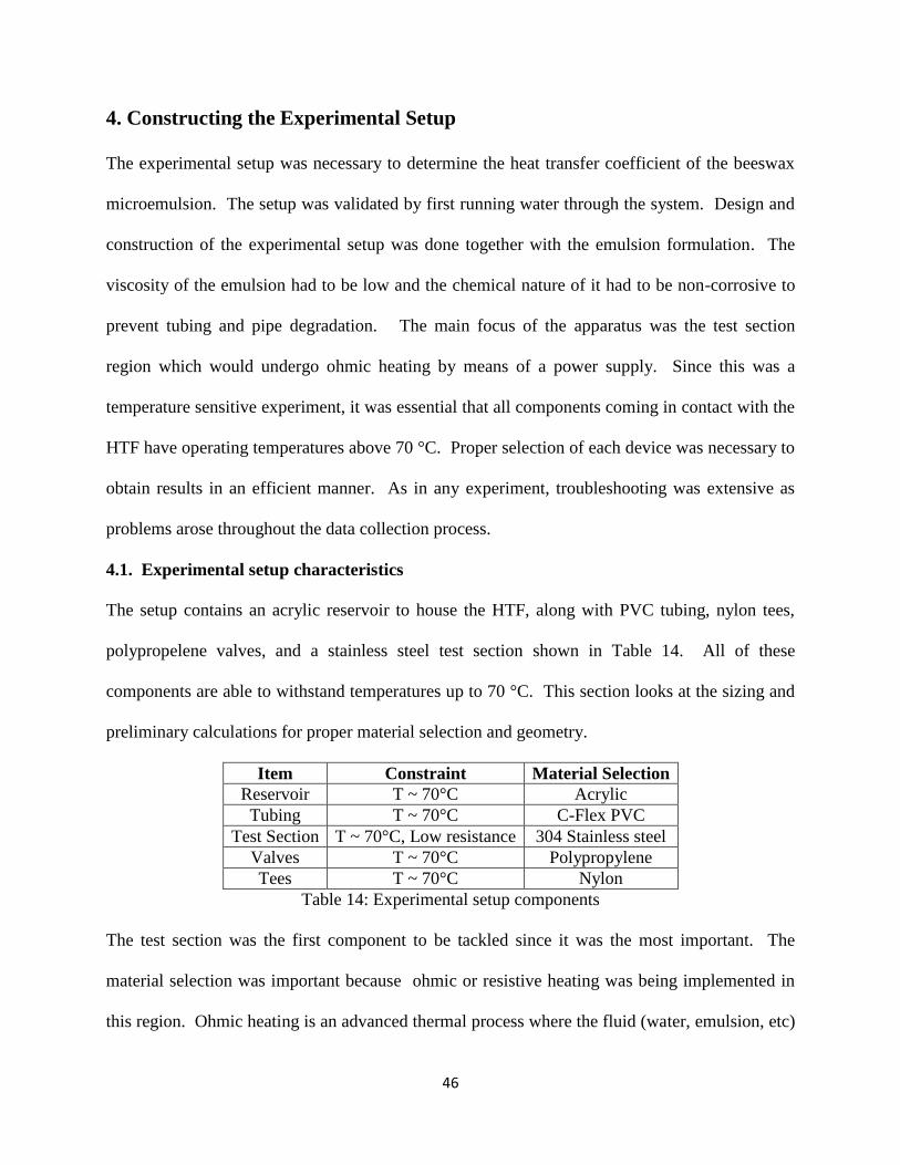
4.1. Experimental setup characteristics
The setup contains an acrylic reservoir to house the HTF, along with PVC tubing, nylon tees,
polypropelene valves, and a stainless steel test section shown in Table 14. All of these
components are able to withstand temperatures up to 70 °C. This section looks at the sizing and
preliminary calculations for proper material selection and geometry.
Item Constraint Material Selection
Reservoir T ~ 70°C Acrylic
Tubing T ~ 70°C C-Flex PVC
Test Section T ~ 70°C, Low resistance 304 Stainless steel
Valves T ~ 70°C Polypropylene
Tees T ~ 70°C Nylon
Table 14: Experimental setup components
The test section was the first component to be tackled since it was the most important. The
material selection was important because ohmic or resistive heating was being implemented in
this region. Ohmic heating is an advanced thermal process where the fluid (water, emulsion, etc)
47
acts as the electrical resistor. The design calls for electrodes to contact the fluid after which
electricity can be conducted through the substance using a power supply with a specified voltage
and amperage range. The HTF will then be heated by means of electrical energy dissipation.
Unlike other methods, it is expected to undergo uniform heating due to the presence of a uniform
heat flux setup. This is the major reason for using this system. Equations were established to
calculate the heat transfer coefficient where uniform heat flux is taking place. The temperature
an ohmic heating can achieve is dictated by the following: 1) electrical conductivity of the fluid,
2) system design, 3) heating time fluid is subjected to, 4) thermophysical properties of the fluid,
5) electrical field strength and constancy, 6) temperature dependence of electrical conductivities,
7) the degree of the interstitial motion in the food, To have a satisfactory setup, the resistance
of the metal must be high with a small wall thickness [23]. The following formula for electrical
resistance was used to select an appropriate material and size:
where:
R = electrical resistance (Ω)
= resistivity of material (Ω-m)
L = length of test section (m)
= cross-sectional area (m2)
To optimize the result for higher electrical resistance, it was necessary to utilize a material with
high resistivity, long length, and small cross-sectional area. This material will heat up and
transfer the thermal energy to the fluid uniformly. Choosing between 304 stainless steel and
inconel 600 was simple, as the first was commercially available, cheaper, and in a small cross-
sectional area. The physical properties and geometry of the 304 stainless steel pipe are shown in
Table 15 which were determined to be adequate for the experiment.
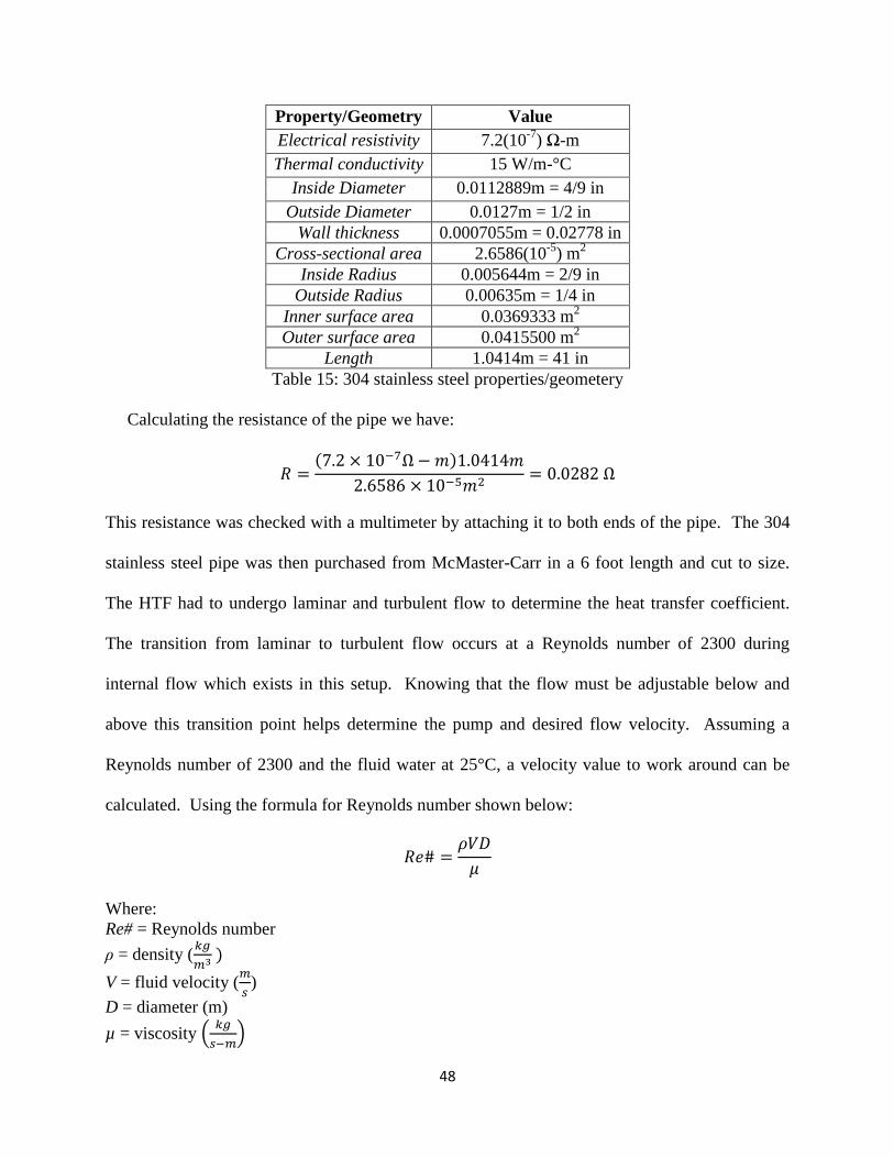
48
Property/Geometry Value
Electrical resistivity 7.2(10-7
) Ω-m
Thermal conductivity 15 W/m-°C
Inside Diameter 0.0112889m = 4/9 in
Outside Diameter 0.0127m = 1/2 in
Wall thickness 0.0007055m = 0.02778 in
Cross-sectional area 2.6586(10-5
) m2
Inside Radius 0.005644m = 2/9 in
Outside Radius 0.00635m = 1/4 in
Inner surface area 0.0369333 m2
Outer surface area 0.0415500 m2
Length 1.0414m = 41 in
Table 15: 304 stainless steel properties/geometery
Calculating the resistance of the pipe we have:
This resistance was checked with a multimeter by attaching it to both ends of the pipe. The 304
stainless steel pipe was then purchased from McMaster-Carr in a 6 foot length and cut to size.
The HTF had to undergo laminar and turbulent flow to determine the heat transfer coefficient.
The transition from laminar to turbulent flow occurs at a Reynolds number of 2300 during
internal flow which exists in this setup. Knowing that the flow must be adjustable below and
above this transition point helps determine the pump and desired flow velocity. Assuming a
Reynolds number of 2300 and the fluid water at 25°C, a velocity value to work around can be
calculated. Using the formula for Reynolds number shown below:
Where:
Re# = Reynolds number
ρ = density (
V = fluid velocity (
)
D = diameter (m)
µ = viscosity
49
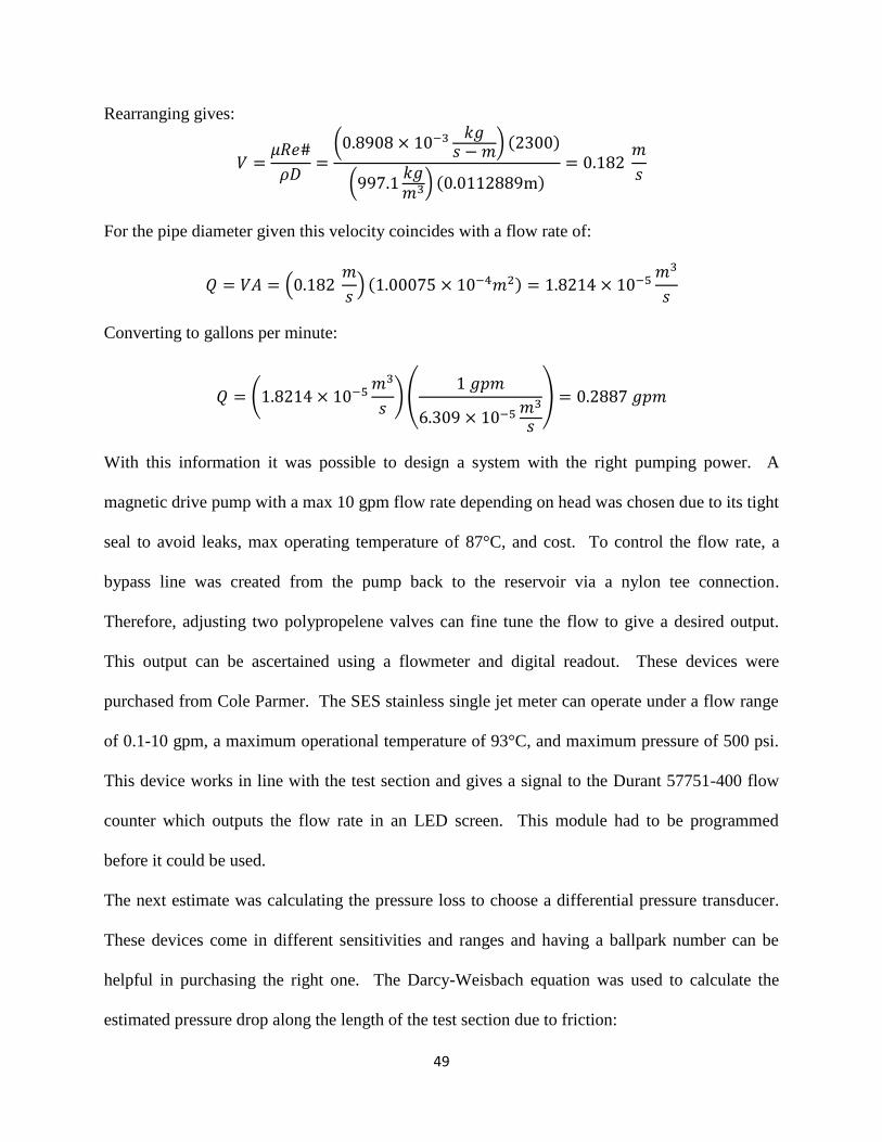
Rearranging gives:
For the pipe diameter given this velocity coincides with a flow rate of:
Converting to gallons per minute:
With this information it was possible to design a system with the right pumping power. A
magnetic drive pump with a max 10 gpm flow rate depending on head was chosen due to its tight
seal to avoid leaks, max operating temperature of 87°C, and cost. To control the flow rate, a
bypass line was created from the pump back to the reservoir via a nylon tee connection.
Therefore, adjusting two polypropelene valves can fine tune the flow to give a desired output.
This output can be ascertained using a flowmeter and digital readout. These devices were
purchased from Cole Parmer. The SES stainless single jet meter can operate under a flow range
of 0.1-10 gpm, a maximum operational temperature of 93°C, and maximum pressure of 500 psi.
This device works in line with the test section and gives a signal to the Durant 57751-400 flow
counter which outputs the flow rate in an LED screen. This module had to be programmed
before it could be used.
The next estimate was calculating the pressure loss to choose a differential pressure transducer.
These devices come in different sensitivities and ranges and having a ballpark number can be
helpful in purchasing the right one. The Darcy-Weisbach equation was used to calculate the
estimated pressure drop along the length of the test section due to friction:
50
Where:
= pressure drop (Pa)
f = friction factor (from Moody's diagram)
L = pipe length (m)
D = diameter (m)
ρ = density (
V = fluid velocity (
)
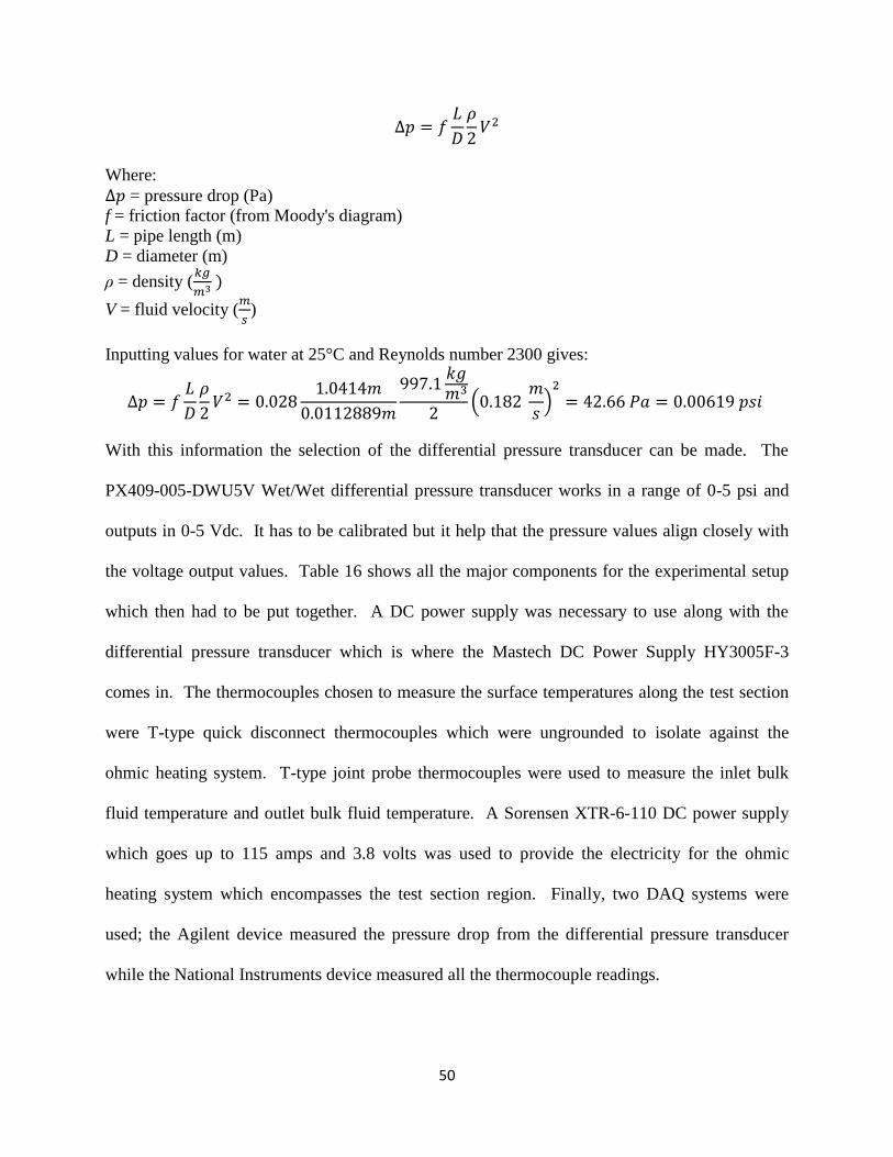
Inputting values for water at 25°C and Reynolds number 2300 gives:
With this information the selection of the differential pressure transducer can be made. The
PX409-005-DWU5V Wet/Wet differential pressure transducer works in a range of 0-5 psi and
outputs in 0-5 Vdc. It has to be calibrated but it help that the pressure values align closely with
the voltage output values. Table 16 shows all the major components for the experimental setup
which then had to be put together. A DC power supply was necessary to use along with the
differential pressure transducer which is where the Mastech DC Power Supply HY3005F-3
comes in. The thermocouples chosen to measure the surface temperatures along the test section
were T-type quick disconnect thermocouples which were ungrounded to isolate against the
ohmic heating system. T-type joint probe thermocouples were used to measure the inlet bulk
fluid temperature and outlet bulk fluid temperature. A Sorensen XTR-6-110 DC power supply
which goes up to 115 amps and 3.8 volts was used to provide the electricity for the ohmic
heating system which encompasses the test section region. Finally, two DAQ systems were
used; the Agilent device measured the pressure drop from the differential pressure transducer
while the National Instruments device measured all the thermocouple readings.
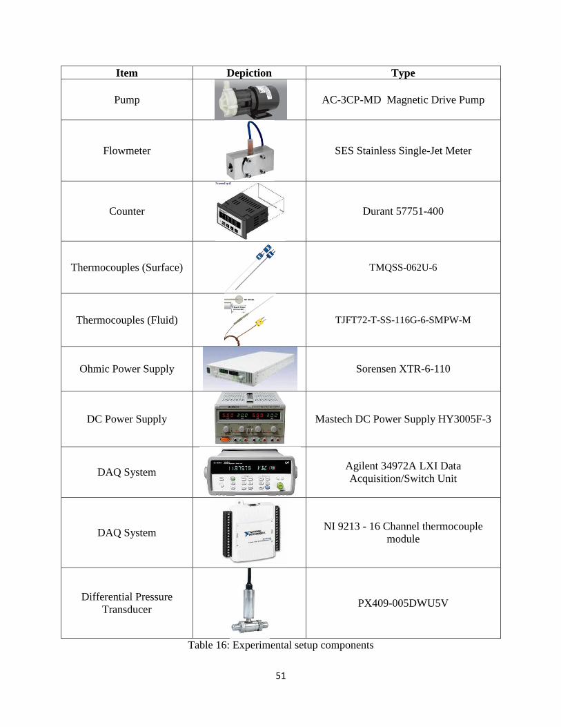
51
Item Depiction Type
Pump
AC-3CP-MD Magnetic Drive Pump
Flowmeter
SES Stainless Single-Jet Meter
Counter
Durant 57751-400
Thermocouples (Surface)
TMQSS-062U-6
Thermocouples (Fluid)
TJFT72-T-SS-116G-6-SMPW-M
Ohmic Power Supply
Sorensen XTR-6-110
DC Power Supply
Mastech DC Power Supply HY3005F-3
DAQ System
Agilent 34972A LXI Data
Acquisition/Switch Unit
DAQ System
NI 9213 - 16 Channel thermocouple
module
Differential Pressure
Transducer
PX409-005DWU5V
Table 16: Experimental setup components

52
4.2. Experimental setup construction
After the major components of the experiment were chosen, sizing of the system was underway.
A tabletop setup was the goal with materials and equipment which could operate at and above
the melting temperature of the beeswax PCM. Figure 33 shows the schematic diagram of the
experimental apparatus. The major components are the PCS reservoir, pump, bypass line,
flowmeter, power supply for ohmic heating, differential pressure transducer, T-type
thermocouples (surface and joint probe), and DAQ system for data logging.
reservoir
valve
valvepump
flowmeterPower supply
Bypas
s li
ne
Differential
pressure
transducer
P
DAQ
System
2 Bulk fluid
thermocouples
6 surface
thermocouples
Figure 33: Schematic diagram of experimental apparatus
The main concern is the test section which is monitored by thermocouples. It will have 6 evenly
spaced thermocouples touching the surface of the stainless steel pipe and 2 thermocouples in the
bulk fluid inlet and outlet. The setup is made to take advantage of heat transfer equations already
established. As with any experiment, a number of minor tweaks had to be made in order to
optimize the system and decrease error in DAQ system readouts. Simple checks had to be
performed periodically to determine the accuracy of the system which will be discussed in the
next chapter. With the components selected and preliminary sizing complete, it was time to
construct the system in a cost effective and efficient manner.

53
Figure 34 shows a Solidworks depiction of the actual experimental apparatus which drew from
the schematic shown earlier. The spacing and geometry of each component is very truthful to
the real setup. Material wise, plywood was used as the base from which to attach components
and structural members. Wood was chosen instead of metal to avoid any interference with the
ohmic heating system along with having high workability. Balsa blocks were appended to the
wood and used as a platform to setup the piping system including test section and flowmeter. An
acrylic stand was made to house the reservoir and pump as well as serve as the basis for many
quick connection points including bypass and resupply lines. Major material choices are shown
in yellow in Figure 34 with temperature and ease of use significant factors.
Figure 34: SolidWorks assembly of experimental apparatus
reservoir
counter Differential
pressure
transducer
power
supply
pump
T-type
thermocouples
test section
wood
balsa
acrylic
PVC
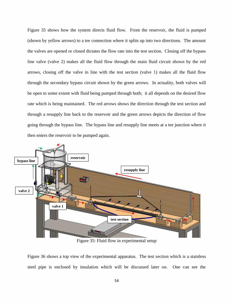
54
Figure 35 shows how the system directs fluid flow. From the reservoir, the fluid is pumped
(shown by yellow arrows) to a tee connection where it splits up into two directions. The amount
the valves are opened or closed dictates the flow rate into the test section. Closing off the bypass
line valve (valve 2) makes all the fluid flow through the main fluid circuit shown by the red
arrows, closing off the valve in line with the test section (valve 1) makes all the fluid flow
through the secondary bypass circuit shown by the green arrows. In actuality, both valves will
be open to some extent with fluid being pumped through both; it all depends on the desired flow
rate which is being maintained. The red arrows shows the direction through the test section and
through a resupply line back to the reservoir and the green arrows depicts the direction of flow
going through the bypass line. The bypass line and resupply line meets at a tee junction where it
then enters the reservoir to be pumped again.
Figure 35: Fluid flow in experimental setup
Figure 36 shows a top view of the experimental apparatus. The test section which is a stainless
steel pipe is enclosed by insulation which will be discussed later on. One can see the
reservoir
resupply line
bypass line
valve 1
valve 2
test section
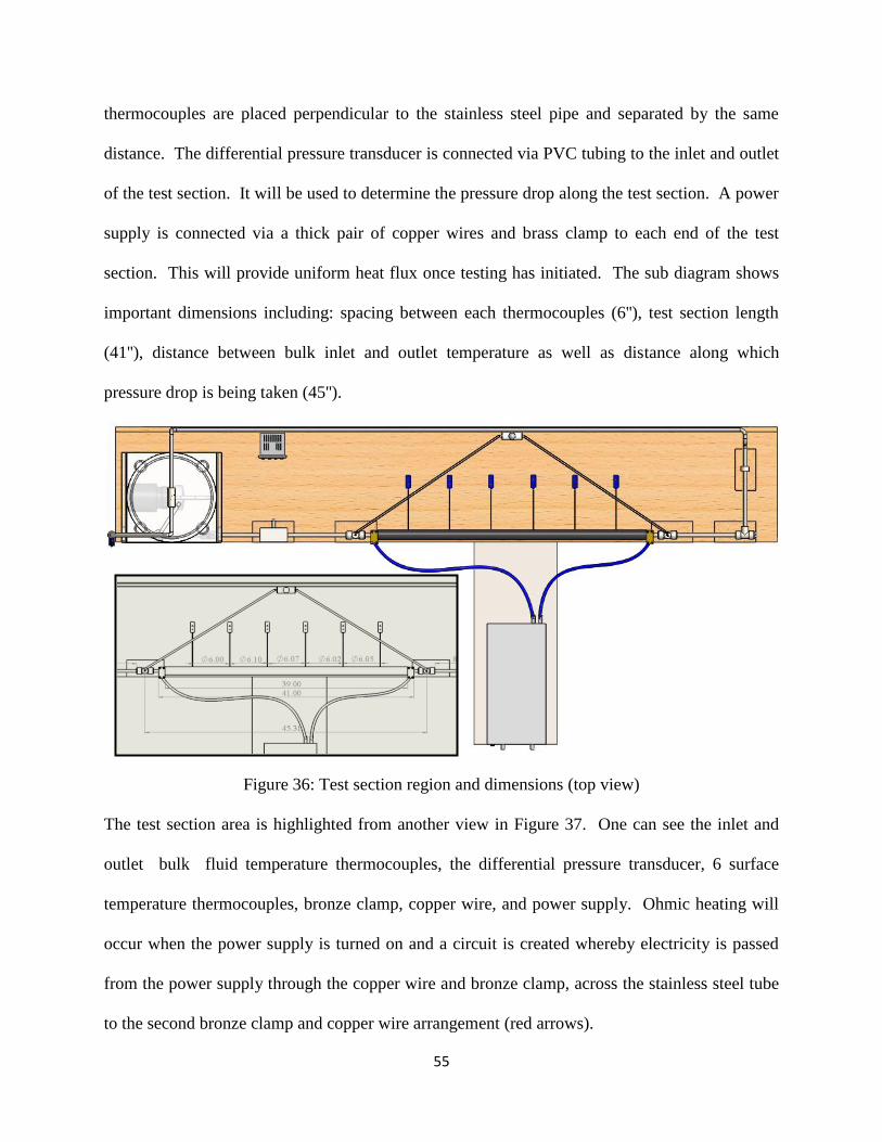
55
thermocouples are placed perpendicular to the stainless steel pipe and separated by the same
distance. The differential pressure transducer is connected via PVC tubing to the inlet and outlet
of the test section. It will be used to determine the pressure drop along the test section. A power
supply is connected via a thick pair of copper wires and brass clamp to each end of the test
section. This will provide uniform heat flux once testing has initiated. The sub diagram shows
important dimensions including: spacing between each thermocouples (6''), test section length
(41''), distance between bulk inlet and outlet temperature as well as distance along which
pressure drop is being taken (45'').
Figure 36: Test section region and dimensions (top view)
The test section area is highlighted from another view in Figure 37. One can see the inlet and
outlet bulk fluid temperature thermocouples, the differential pressure transducer, 6 surface
temperature thermocouples, bronze clamp, copper wire, and power supply. Ohmic heating will
occur when the power supply is turned on and a circuit is created whereby electricity is passed
from the power supply through the copper wire and bronze clamp, across the stainless steel tube
to the second bronze clamp and copper wire arrangement (red arrows).
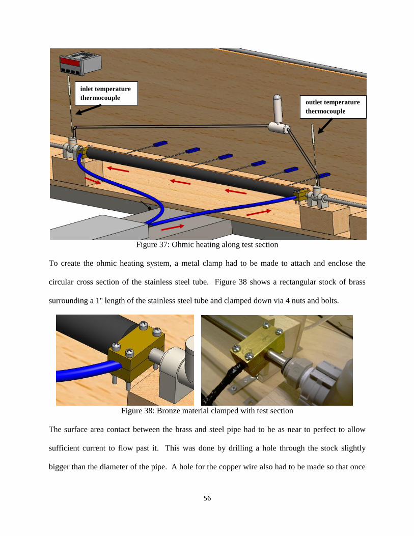
56
Figure 37: Ohmic heating along test section
To create the ohmic heating system, a metal clamp had to be made to attach and enclose the
circular cross section of the stainless steel tube. Figure 38 shows a rectangular stock of brass
surrounding a 1'' length of the stainless steel tube and clamped down via 4 nuts and bolts.
Figure 38: Bronze material clamped with test section
The surface area contact between the brass and steel pipe had to be as near to perfect to allow
sufficient current to flow past it. This was done by drilling a hole through the stock slightly
bigger than the diameter of the pipe. A hole for the copper wire also had to be made so that once
inlet temperature
thermocouple outlet temperature
thermocouple
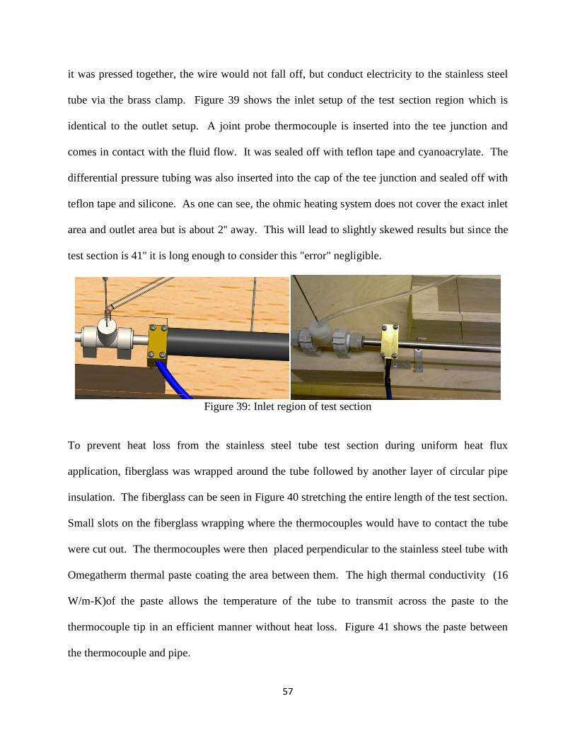
57
it was pressed together, the wire would not fall off, but conduct electricity to the stainless steel
tube via the brass clamp. Figure 39 shows the inlet setup of the test section region which is
identical to the outlet setup. A joint probe thermocouple is inserted into the tee junction and
comes in contact with the fluid flow. It was sealed off with teflon tape and cyanoacrylate. The
differential pressure tubing was also inserted into the cap of the tee junction and sealed off with
teflon tape and silicone. As one can see, the ohmic heating system does not cover the exact inlet
area and outlet area but is about 2'' away. This will lead to slightly skewed results but since the
test section is 41'' it is long enough to consider this "error" negligible.
Figure 39: Inlet region of test section
To prevent heat loss from the stainless steel tube test section during uniform heat flux
application, fiberglass was wrapped around the tube followed by another layer of circular pipe
insulation. The fiberglass can be seen in Figure 40 stretching the entire length of the test section.
Small slots on the fiberglass wrapping where the thermocouples would have to contact the tube
were cut out. The thermocouples were then placed perpendicular to the stainless steel tube with
Omegatherm thermal paste coating the area between them. The high thermal conductivity (16
W/m-K)of the paste allows the temperature of the tube to transmit across the paste to the
thermocouple tip in an efficient manner without heat loss. Figure 41 shows the paste between
the thermocouple and pipe.
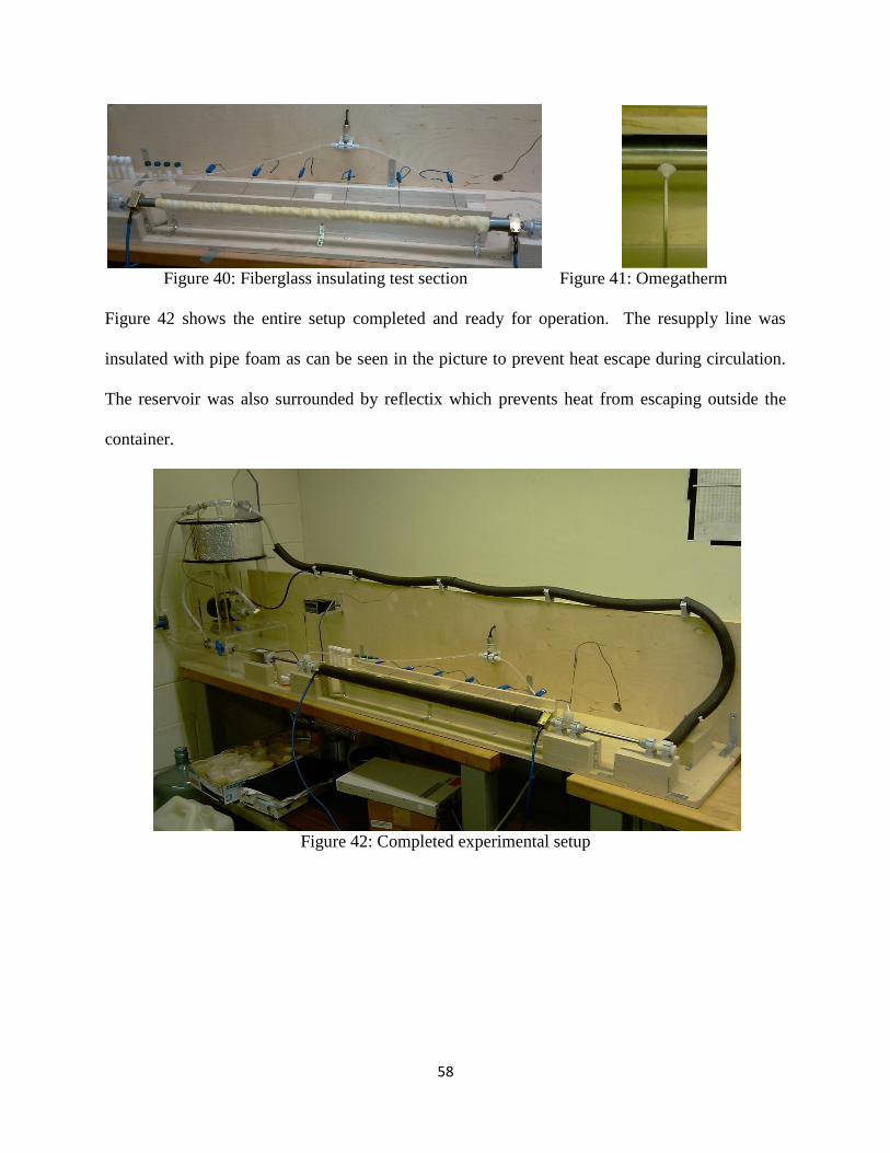
58
Figure 40: Fiberglass insulating test section Figure 41: Omegatherm
Figure 42 shows the entire setup completed and ready for operation. The resupply line was
insulated with pipe foam as can be seen in the picture to prevent heat escape during circulation.
The reservoir was also surrounded by reflectix which prevents heat from escaping outside the
container.
Figure 42: Completed experimental setup
59
5. Results for Water & Beeswax microemulsion
5.1. Setting up data collection & analysis
After the experimental setup was complete, it was time to run experiments with water as the
working fluid. The results from water will be compared to those expected from heat transfer
equations for uniform heat flux. If they "match up" then one can proclaim that the experimental
setup is adequate to determine the heat transfer coefficient for the beeswax microemulsion. To
obtain results, the pump was plugged in, and the desired flow rate was established by adjusting
the bypass valves. Once a fixed flow rate was reached, it was then time to turn on the power
supply to the desired power output. This was accomplished by adjusting the amperage and
voltage. As expected, increasing the power increases the surface heat flux over the test section
which leads to an increasing temperature change from inlet to outlet. Since the first scenario was
just distilled water without a phase change, there was no need to reach a certain melting
temperature. The experiment was run by gradually increasing the power to the test section and
recording the thermocouple readings, both bulk fluid and surface temperature. One problem
which occurred often was a changing flow rate as the HTF temperature increased. As the
temperature of the water increased, the viscosity decreased and thus there was less friction
between the pipe wall and fluid. Constant adjusting of the valves had to be made to keep the
flow rate constant otherwise the results would be meaningless. The governing equation which
will be used is found in any heat transfer textbook [24]:
Where:
= Power input (W)
= bulk fluid temperature at location x from Tmi (°C)
= surface temperature of test section at location x from Tmi (°C)
= surface area of test section ( )
= local heat transfer coefficient at distance x from test section (
)

60
Rearranging, we can get the local heat transfer coefficient as:
Where:
=VI= surface heat flux (
)
The heat transfer coefficient is time dependent since the working fluid will be heating up
throughout the course of the experiment and specific heat values will be changing. Power input
into the test section will also change as the voltage and amperage are adjusted which will lead to
temperature and surface heat flux changes. Figure 43 shows the thermocouple designations
which includes two end joint probe thermocouples and six surface probe thermocouples.
Figure 43: Thermocouple designations
In this investigation, the local heat transfer coefficients will be calculated for each zone or
section of the test section where thermocouples are present. Basically, h values will be
determined at each thermocouple location from the inlet and averaged over time to give an h for
the entire test section. T2 is located 4.75'' away from Tmi, T3 is 10.75'' away, T4 is 16.75'' away,
T5 is 22.75'' away, T6 is 28.75'' away, and T7 is 34.75'' away from Tmi. The following procedure
will be used to determine the heat transfer coefficients for each test scenario:
1. HTF is placed into the reservoir and settles throughout the system.
2. Pump is powered on and a flow rate in gpm is set and maintained throughout the experiment
by adjusting the flow valves.
Tmi Tmo
T2 T3 T4 T5 T6 T7
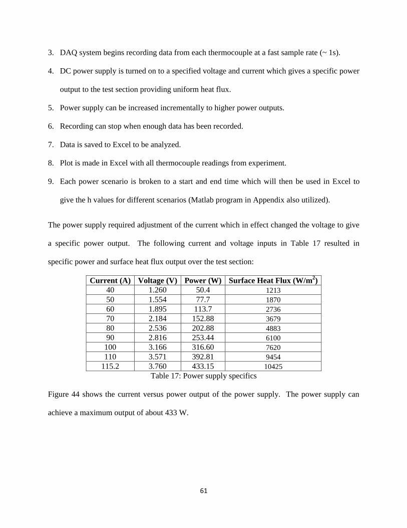
61
3. DAQ system begins recording data from each thermocouple at a fast sample rate (~ 1s).
4. DC power supply is turned on to a specified voltage and current which gives a specific power
output to the test section providing uniform heat flux.
5. Power supply can be increased incrementally to higher power outputs.
6. Recording can stop when enough data has been recorded.
7. Data is saved to Excel to be analyzed.
8. Plot is made in Excel with all thermocouple readings from experiment.
9. Each power scenario is broken to a start and end time which will then be used in Excel to
give the h values for different scenarios (Matlab program in Appendix also utilized).
The power supply required adjustment of the current which in effect changed the voltage to give
a specific power output. The following current and voltage inputs in Table 17 resulted in
specific power and surface heat flux output over the test section:
Current (A) Voltage (V) Power (W) Surface Heat Flux (W/m2)
40 1.260 50.4 1213
50 1.554 77.7 1870
60 1.895 113.7 2736
70 2.184 152.88 3679
80 2.536 202.88 4883
90 2.816 253.44 6100
100 3.166 316.60 7620
110 3.571 392.81 9454
115.2 3.760 433.15 10425
Table 17: Power supply specifics
Figure 44 shows the current versus power output of the power supply. The power supply can
achieve a maximum output of about 433 W.
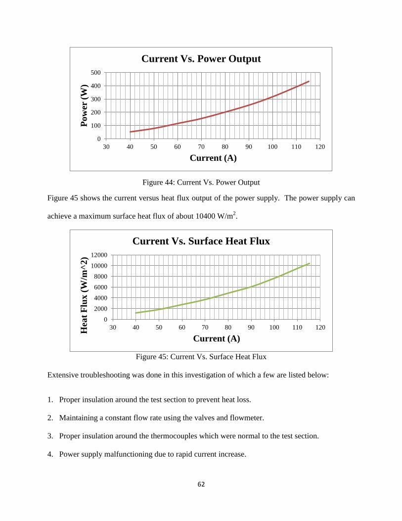
62
Figure 44: Current Vs. Power Output
Figure 45 shows the current versus heat flux output of the power supply. The power supply can
achieve a maximum surface heat flux of about 10400 W/m2.
Figure 45: Current Vs. Surface Heat Flux
Extensive troubleshooting was done in this investigation of which a few are listed below:
1. Proper insulation around the test section to prevent heat loss.
2. Maintaining a constant flow rate using the valves and flowmeter.
3. Proper insulation around the thermocouples which were normal to the test section.
4. Power supply malfunctioning due to rapid current increase.
0
100
200
300
400
500
30 40 50 60 70 80 90 100 110 120
Po
wer
(W
)
Current (A)
Current Vs. Power Output
0
2000
4000
6000
8000
10000
12000
30 40 50 60 70 80 90 100 110 120
Hea
t F
lux
(W
/m^
2)
Current (A)
Current Vs. Surface Heat Flux
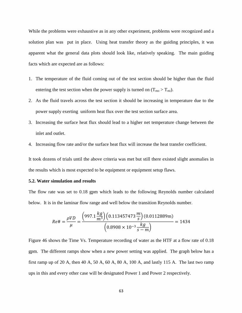
63
While the problems were exhaustive as in any other experiment, problems were recognized and a
solution plan was put in place. Using heat transfer theory as the guiding principles, it was
apparent what the general data plots should look like, relatively speaking. The main guiding
facts which are expected are as follows:
1. The temperature of the fluid coming out of the test section should be higher than the fluid
entering the test section when the power supply is turned on (Tmo > Tmi).
2. As the fluid travels across the test section it should be increasing in temperature due to the
power supply exerting uniform heat flux over the test section surface area.
3. Increasing the surface heat flux should lead to a higher net temperature change between the
inlet and outlet.
4. Increasing flow rate and/or the surface heat flux will increase the heat transfer coefficient.
It took dozens of trials until the above criteria was met but still there existed slight anomalies in
the results which is most expected to be equipment or equipment setup flaws.
5.2. Water simulation and results
The flow rate was set to 0.18 gpm which leads to the following Reynolds number calculated
below. It is in the laminar flow range and well below the transition Reynolds number.
Figure 46 shows the Time Vs. Temperature recording of water as the HTF at a flow rate of 0.18
gpm. The different ramps show when a new power setting was applied. The graph below has a
first ramp up of 20 A, then 40 A, 50 A, 60 A, 80 A, 100 A, and lastly 115 A. The last two ramp
ups in this and every other case will be designated Power 1 and Power 2 respectively.
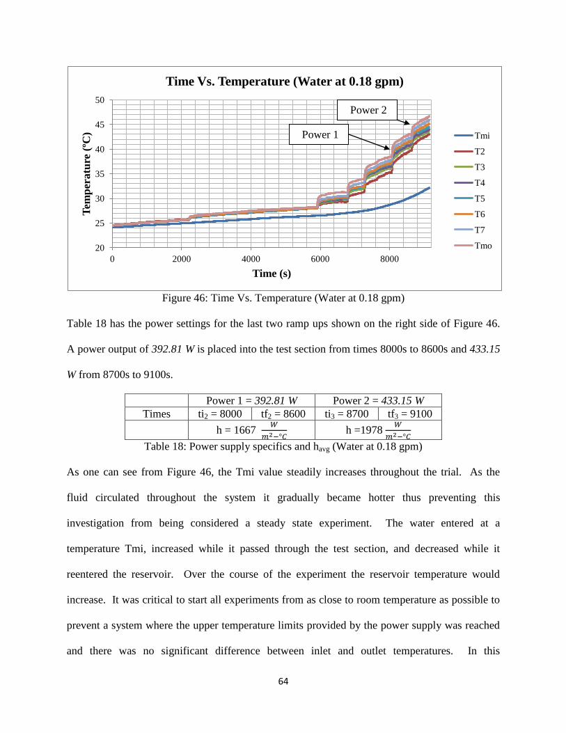
64
Figure 46: Time Vs. Temperature (Water at 0.18 gpm)
Table 18 has the power settings for the last two ramp ups shown on the right side of Figure 46.
A power output of 392.81 W is placed into the test section from times 8000s to 8600s and 433.15
W from 8700s to 9100s.
Power 1 = 392.81 W Power 2 = 433.15 W
Times ti2 = 8000 tf2 = 8600 ti3 = 8700 tf3 = 9100
h = 1667
h =1978
Table 18: Power supply specifics and havg (Water at 0.18 gpm)
As one can see from Figure 46, the Tmi value steadily increases throughout the trial. As the
fluid circulated throughout the system it gradually became hotter thus preventing this
investigation from being considered a steady state experiment. The water entered at a
temperature Tmi, increased while it passed through the test section, and decreased while it
reentered the reservoir. Over the course of the experiment the reservoir temperature would
increase. It was critical to start all experiments from as close to room temperature as possible to
prevent a system where the upper temperature limits provided by the power supply was reached
and there was no significant difference between inlet and outlet temperatures. In this
20
25
30
35
40
45
50
0 2000 4000 6000 8000
Tem
per
atu
re (
ºC)
Time (s)
Time Vs. Temperature (Water at 0.18 gpm)
Tmi
T2
T3
T4
T5
T6
T7
Tmo
Power 2
Power 1
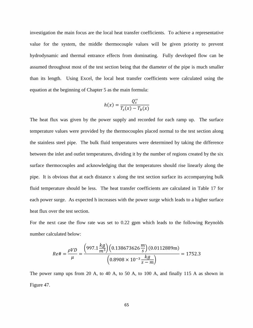
65
investigation the main focus are the local heat transfer coefficients. To achieve a representative
value for the system, the middle thermocouple values will be given priority to prevent
hydrodynamic and thermal entrance effects from dominating. Fully developed flow can be
assumed throughout most of the test section being that the diameter of the pipe is much smaller
than its length. Using Excel, the local heat transfer coefficients were calculated using the
equation at the beginning of Chapter 5 as the main formula:
The heat flux was given by the power supply and recorded for each ramp up. The surface
temperature values were provided by the thermocouples placed normal to the test section along
the stainless steel pipe. The bulk fluid temperatures were determined by taking the difference
between the inlet and outlet temperatures, dividing it by the number of regions created by the six
surface thermocouples and acknowledging that the temperatures should rise linearly along the
pipe. It is obvious that at each distance x along the test section surface its accompanying bulk
fluid temperature should be less. The heat transfer coefficients are calculated in Table 17 for
each power surge. As expected h increases with the power surge which leads to a higher surface
heat flux over the test section.
For the next case the flow rate was set to 0.22 gpm which leads to the following Reynolds
number calculated below:
The power ramp ups from 20 A, to 40 A, to 50 A, to 100 A, and finally 115 A as shown in
Figure 47.
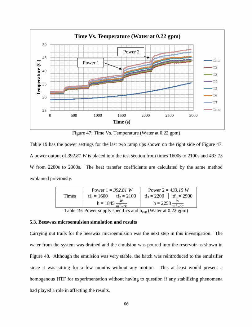
66
Figure 47: Time Vs. Temperature (Water at 0.22 gpm)
Table 19 has the power settings for the last two ramp ups shown on the right side of Figure 47.
A power output of 392.81 W is placed into the test section from times 1600s to 2100s and 433.15
W from 2200s to 2900s. The heat transfer coefficients are calculated by the same method
explained previously.
Power 1 = 392.81 W Power 2 = 433.15 W
Times ti2 = 1600 tf2 = 2100 ti3 = 2200 tf3 = 2900
h = 1845
h = 2253
Table 19: Power supply specifics and havg (Water at 0.22 gpm)
5.3. Beeswax microemulsion simulation and results
Carrying out trails for the beeswax microemulsion was the next step in this investigation. The
water from the system was drained and the emulsion was poured into the reservoir as shown in
Figure 48. Although the emulsion was very stable, the batch was reintroduced to the emulsifier
since it was sitting for a few months without any motion. This at least would present a
homogenous HTF for experimentation without having to question if any stabilizing phenomena
had played a role in affecting the results.
25
30
35
40
45
50
0 500 1000 1500 2000 2500 3000
Tem
per
atu
re (
C)
Time (s)
Time Vs. Temperature (Water at 0.22 gpm)
Tmi
T2
T3
T4
T5
T6
T7
Tmo
Power 2
Power 1
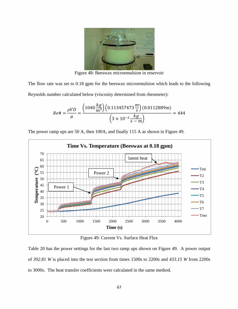
67
Figure 48: Beeswax microemulsion in reservoir
The flow rate was set to 0.18 gpm for the beeswax microemulsion which leads to the following
Reynolds number calculated below (viscosity determined from rheometer):
The power ramp ups are 50 A, then 100A, and finally 115 A as shown in Figure 49.
Figure 49: Current Vs. Surface Heat Flux
Table 20 has the power settings for the last two ramp ups shown on Figure 49. A power output
of 392.81 W is placed into the test section from times 1500s to 2200s and 433.15 W from 2200s
to 3000s. The heat transfer coefficients were calculated in the same method.
20
25
30
35
40
45
50
55
60
65
70
0 500 1000 1500 2000 2500 3000 3500 4000
Tem
pera
ture
(°
C)
Time (s)
Time Vs. Temperature (Beeswax at 0.18 gpm)
Tmi
T2
T3
T4
T5
T6
T7
Tmo
Power 2
Power 1
latent heat
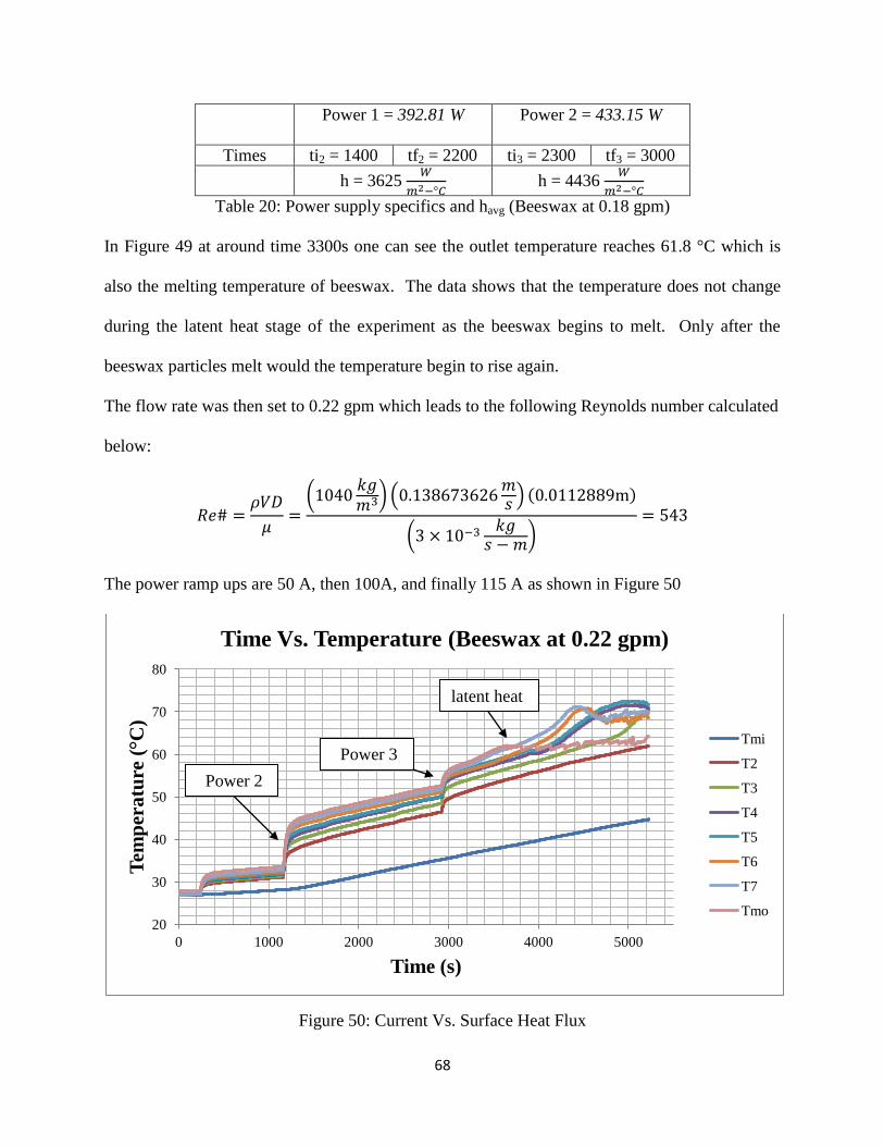
68
Power 1 = 392.81 W Power 2 = 433.15 W
Times ti2 = 1400 tf2 = 2200 ti3 = 2300 tf3 = 3000
h = 3625
h = 4436
Table 20: Power supply specifics and havg (Beeswax at 0.18 gpm)
In Figure 49 at around time 3300s one can see the outlet temperature reaches 61.8 °C which is
also the melting temperature of beeswax. The data shows that the temperature does not change
during the latent heat stage of the experiment as the beeswax begins to melt. Only after the
beeswax particles melt would the temperature begin to rise again.
The flow rate was then set to 0.22 gpm which leads to the following Reynolds number calculated
below:
The power ramp ups are 50 A, then 100A, and finally 115 A as shown in Figure 50
Figure 50: Current Vs. Surface Heat Flux
20
30
40
50
60
70
80
0 1000 2000 3000 4000 5000
Tem
per
atu
re (°C
)
Time (s)
Time Vs. Temperature (Beeswax at 0.22 gpm)
Tmi
T2
T3
T4
T5
T6
T7
Tmo
Power 3
Power 2
latent heat
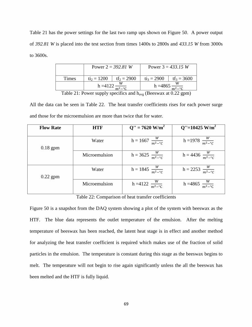
69
Table 21 has the power settings for the last two ramp ups shown on Figure 50. A power output
of 392.81 W is placed into the test section from times 1400s to 2800s and 433.15 W from 3000s
to 3600s.
Power 2 = 392.81 W Power 3 = 433.15 W
Times ti2 = 1200 tf2 = 2900 ti3 = 2900 tf3 = 3600
h =4122
h =4865
Table 21: Power supply specifics and havg (Beeswax at 0.22 gpm)
All the data can be seen in Table 22. The heat transfer coefficients rises for each power surge
and those for the microemulsion are more than twice that for water.
Flow Rate HTF Q'' = 7620 W/m2 Q''=10425 W/m
2
0.18 gpm
Water h = 1667
h =1978
Microemulsion h = 3625
h = 4436
0.22 gpm
Water h = 1845
h = 2253
Microemulsion h =4122
h =4865
Table 22: Comparison of heat transfer coefficients
Figure 50 is a snapshot from the DAQ system showing a plot of the system with beeswax as the
HTF. The blue data represents the outlet temperature of the emulsion. After the melting
temperature of beeswax has been reached, the latent heat stage is in effect and another method
for analyzing the heat transfer coefficient is required which makes use of the fraction of solid
particles in the emulsion. The temperature is constant during this stage as the beeswax begins to
melt. The temperature will not begin to rise again significantly unless the all the beeswax has
been melted and the HTF is fully liquid.
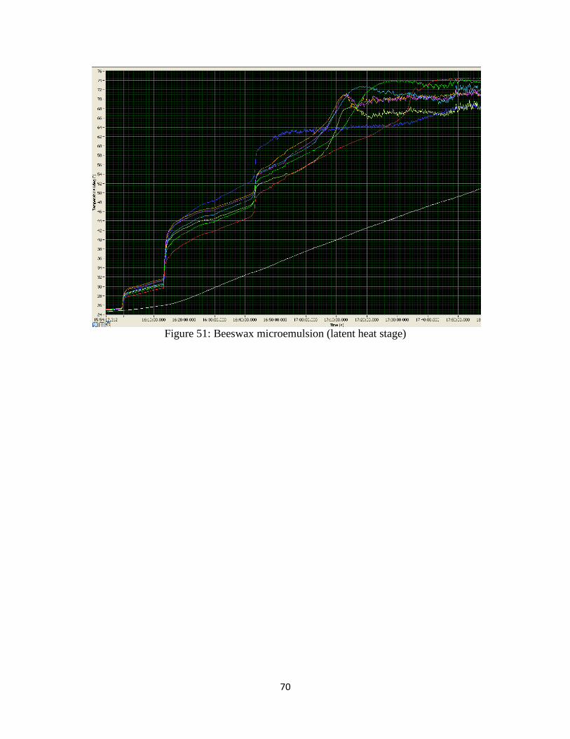
70
Figure 51: Beeswax microemulsion (latent heat stage)
71
6. Conclusion
This investigation saw the formulation of a Phase Change Slurry, the analysis of its stability
characteristics and thermophysical properties, and the calculation of its heat transfer coefficient.
The emulsion created in this experiment had 10% beeswax by weight with stabilizing surfactants
surrounding it in a distilled water environment. The emulsion was pumpable and possessed low
viscosity. An experimental setup was created to determine the heat transfer coefficient of this
microemulsion and comparing it to water in the sensible heat range. The setup employed
thermocouples to record temperature data which may then be used to calculate the heat transfer
coefficient. The result showed that the heat transfer coefficients of the beeswax microemulsion
was more than two times that of water at the same flow rate. Two cases in the laminar flow
region were done, one at 0.18 gpm and the other at 0.22 gpm. The experiment also proved that
the latent heat abilities were inherent in the emulsion. Once the temperature of the system
reached the melting temperature of beeswax, there was little to no temperature change for some
time. All the beeswax particles needed to melt before the temperature of the emulsion would
further increase. Further work is necessary to determine the charging and discharging rates of
this emulsion in comparison to water and also the heat transfer coefficient during the latent heat
stage. PCMs are proving to be very fruitful for thermal energy storage and once its economical
ability has been reached, one can expect widespread implementation in residential, commercial,
and other applications.
72
References
[1] M. Ravikumar and Dr. Pss. Srinivasan, “Phase change material as a thermal energy storage
material for cooling of building,” Journal of Theoretical and Applied Information Technology,
(2008)
[2] Atul Sharma, V.V. Tyagi, C.R. Chen, and D. Buddhi, “Review on thermal energy storage
with phase change materials and applications,” Renewable and Sustainable Energy Reviews, Vol.
13, pp. 318-345, (2009)
[3] A. Pasupathy, R. Velraj, and R.V. Seeniraj, “Phase change material-based building
architecture for thermal management in residential and commercial establishments,” Renewable
and Sustainable Energy Reviews, Vol. 12, pp. 39-64, (2008)
[4] A. Heinz and W. Streicher, “Application of phase change materials and PCM-slurries for
thermal energy storage,” Institute of Thermal Engineering, (2006)
[5] Justin Ning-Wei Chiu, Dr. Viktoria Martin, and Prof. Fredrik Setterwall, “A review of
thermal energy storage systems with salt hydrate phase change materials for comfort cooling,”
KTH – Department of Energy Technology, Sweden
[6] Murat Kenisarin and Khamid Mahkamov, “Solar energy storage using phase change
materials,” Renewable and Sustainable Energy Reviews, Vol. 11, pp. 1913-1965, (2007)
[7] A. Abhat, “Short term thermal energy storage,” Revue Phys. Appl., Vol 15, pp 477-501,
(1980)
[8] Astrid Wille and Volkmar Lottner, “R & D programme on thermal energy storage in
Germany,” 10th
Int. Conference on Thermal Energy Storage, Ecostock 2006
[9] Manish Goel, S.K. Roy, and S. Sengupta, “Laminar forced convection heat transfer in
microencapsulated phase change material suspensions,” International Journal of Heat Mass
Transfer, Vol. 37, No. 4, pp. 593-604, (1994)
[10] Li Huang and Christian Dotsch, “Paraffin/Water emulsion for cold storage and distribution
applications,” IEA/ECES Annex 18, The Fifth Workshop and Expert Meeting, (2008)
[11] Hiveharvest.com. "Beeswax, honey, and beeswax candles made by honeybees at Tahuya
River Apiaries
[12] Richard Grove. "Notes on making cola," Issue 2, Wilmington, Delaware, (2005)
[13] ICI Americas Inc. "The HLB system a time saving guide to emulsifier selection,"
Chemmunique, (1980)

73
[14] W.M. Wan Rusmawati, K. Dzulnmkefly, W.H. Lim, and S. Hamdan. "Emulsion properties
of mixed Tween20-Span20 in non-aqueous system," Pertanika J. Sci. & Technol, Vol. 10. pp.
153-160, (2002)
[15] Silverson. "Multi-Purpose High Shear Laboratory Mixers," Silverson Machines Ltd. pp. 4-
5, (2011)
[16] Dispersion Analyser LUMiSizer. "The complete Dispersion Lab in one Instrument," L.U.M.
GmbH, (2011)
[17] Gonul Kocak. 2010. “Producing micro and nano fibers having high water holding capacity
from tomato and wheat waste products and using them in model foods,” Master’s Thesis, Middle
East Technical University, Turkey
[18] "Methods to measure stability of dispersions: Adaptive Instruments," Benelux Scientific lab
technology for research and innovation
[19] Torsten Detloff, Titus Sobisch, and Dietmar Lerche. "Particle size distribution by space or
time dependent extinction profiles obtained by analytical centrifugation (concentrated systems),"
Powder Technology, Vol. 174, pp. 50-55, (2007)
[20] V. Andre, N. Willenbacher, H. Debus, L. Borger, P. Fernandez, T. Frechen, and J. Rieger,
“Prediction of emulsion stability: facts and myth,” Cosmetics and Toiletries Manufature
Worldwide
[21] Jorge L. Alvarado, Barclay G. Jones, Charles P. Marsh, David A. Kessler, Chang W. Sohn,
Carl A. Feickert, Gary E. Phetteplace, Eric D. Crowley, Ryan J. Franks, and Thomas A. Carlson
2008. “Thermal performance of microencapsulated phase change material slurry,” Construction
Engineering Research Laboratory, US Army Corps of Engineers, Washington D.C.
[22] Pruitipong Thaicham, “Heat transport in a three-stage thermal energy system using phase
change material slurries,” ScienceAsia, Vol. 34, pp. 223-228, (2008)
[23] Destinee R. Anderson 2008. “Ohmic heating as an alternative food processing technology,”
Master’s Thesis, Kansas State University, Kansas
[24] Latif M. Jji. "Heat Transfer Essentials: A Textbook," Begell House, Inc, New York, 2nd
Edition, (2002)

74
Appendix
MATLAB PROGRAM clear clc
%Section Properties% di=4/9*0.0254; %Inner Pipe Diameter [m]% do=0.5*0.0254; %Outer Pipe Diameter [m]% L=39.5*0.0254; %Length of Section [m]% P=pi*do; %Perimeter [m]% As=P*L; %Surface Area [m^2]; Ac=pi*di^2/4; %Cross-Sectional Area [m^2]% delx=[4.75,10.75,16.75,22.75,28.75,34.75]*0.0254; %Distance of Each %Thermocouple to Tmi%
%Flow Properties% rho=990; %Density of HTF [kg/m^3]% Vdot=0.18*6.30901964*10^-5; %Volume Flow Rate [m^3/s]; mdot=rho*Vdot; %Mass Flow Rate [kg/s]% A = input('Input value for A: ');%Start of first heat flux value B = input('Input value for B: ');%End of first heat flux value C = input('Input value for C: ');%Start of second heat flux value D = input('Input value for D: ');%End of second heat flux value E = input('Input value for E: ');%Start of third heat flux value F = input('Input value for F: ');%End of third heat flux value
Bee=xlsread('Thesis_water_0.18.xlsx'); t=Bee(:,1); Tmi=Bee(:,2); Ts1=Bee(:,3); Ts2=Bee(:,4); Ts3=Bee(:,5); Ts4=Bee(:,6); Ts5=Bee(:,7); Ts6=Bee(:,8); Tmo=Bee(:,9);
tq1=zeros(length(A:B),1); Tmiq1=zeros(length(A:B),1); Ts1q1=zeros(length(A:B),1); Ts2q1=zeros(length(A:B),1); Ts3q1=zeros(length(A:B),1); Ts4q1=zeros(length(A:B),1); Ts5q1=zeros(length(A:B),1); Ts6q1=zeros(length(A:B),1); Tmoq1=zeros(length(A:B),1); cpq1=zeros(length(A:B),1); htaq1Ts1=zeros(length(A:B),1); htaq1Ts2=zeros(length(A:B),1); htaq1Ts3=zeros(length(A:B),1); htaq1Ts4=zeros(length(A:B),1); htaq1Ts5=zeros(length(A:B),1); htaq1Ts6=zeros(length(A:B),1);

75
%First Heat Flux% j=0; for i=A:B j=j+1; I1=80; %Current First Jump [A]% V1=2.6634; %Voltage First Jump [V]% Q1=I1*V1; %First Power Input into Section [W]% Qs1=Q1/As; %First Heat Flux [W/m^2]% tq1(j)=t(i); %First Heat Flux Time Period [s]% Tmiq1(j)=Tmi(i); %First Heat Flux Tmi [C]% Ts1q1(j)=Ts1(i); %First Heat Flux Ts1 [C]% Ts2q1(j)=Ts2(i); %First Heat Flux Ts2 [C]% Ts3q1(j)=Ts3(i); %First Heat Flux Ts3 [C]% Ts4q1(j)=Ts4(i); %First Heat Flux Ts4 [C]% Ts5q1(j)=Ts5(i); %First Heat Flux Ts5 [C]% Ts6q1(j)=Ts6(i); %First Heat Flux Ts6 [C]% Tmoq1(j)=Tmo(i); %First Heat Flux Tmo [C]% cpq1(j)=Q1/mdot/(Tmoq1(j,1)-Tmiq1(j,1)); %First Heat Flux Cp [J/Kg-K]% htaq1Ts1(j)=((Ts1q1(j)-Tmiq1(j))/Qs1-P*delx(1)/mdot/cpq1(j))^(-1); %Heat
Transfer Coefficient for First Heat Flux Case at Each Time at Ts1 [W/m-K]% htaq1Ts2(j)=((Ts2q1(j)-Tmiq1(j))/Qs1-P*delx(2)/mdot/cpq1(j))^(-1); %Heat
Transfer Coefficient for First Heat Flux Case at Each Time at Ts2 [W/m-K]% htaq1Ts3(j)=((Ts3q1(j)-Tmiq1(j))/Qs1-P*delx(3)/mdot/cpq1(j))^(-1); %Heat
Transfer Coefficient for First Heat Flux Case at Each Time at Ts3 [W/m-K]% htaq1Ts4(j)=((Ts4q1(j)-Tmiq1(j))/Qs1-P*delx(4)/mdot/cpq1(j))^(-1); %Heat
Transfer Coefficient for First Heat Flux Case at Each Time at Ts4 [W/m-K]% htaq1Ts5(j)=((Ts5q1(j)-Tmiq1(j))/Qs1-P*delx(5)/mdot/cpq1(j))^(-1); %Heat
Transfer Coefficient for First Heat Flux Case at Each Time at Ts5 [W/m-K]% htaq1Ts6(j)=((Ts6q1(j)-Tmiq1(j))/Qs1-P*delx(6)/mdot/cpq1(j))^(-1); %Heat
Transfer Coefficient for First Heat Flux Case at Each Time at Ts6 [W/m-K]% end
htaveq1Ts1=0; %Time-Averaged Heat Transfer Coefficient for First Heat Flux
Case at Ts1 [W/m-K]% htaveq1Ts2=0; %Time-Averaged Heat Transfer Coefficient for First Heat Flux
Case at Ts2 [W/m-K]% htaveq1Ts3=0; %Time-Averaged Heat Transfer Coefficient for First Heat Flux
Case at Ts3 [W/m-K]% htaveq1Ts4=0; %Time-Averaged Heat Transfer Coefficient for First Heat Flux
Case at Ts4 [W/m-K]% htaveq1Ts5=0; %Time-Averaged Heat Transfer Coefficient for First Heat Flux
Case at Ts5 [W/m-K]% htaveq1Ts6=0; %Time-Averaged Heat Transfer Coefficient for First Heat Flux
Case at Ts6 [W/m-K]%
for j=1:length(A:B)-1 htaqTs1=(tq1(length(A:B))-tq1(1))^(-
1)*0.5*(htaq1Ts1(j)+htaq1Ts1(j+1))*(tq1(j+1)-tq1(j)); htaqTs2=(tq1(length(A:B))-tq1(1))^(-
1)*0.5*(htaq1Ts2(j)+htaq1Ts2(j+1))*(tq1(j+1)-tq1(j)); htaqTs3=(tq1(length(A:B))-tq1(1))^(-
1)*0.5*(htaq1Ts3(j)+htaq1Ts3(j+1))*(tq1(j+1)-tq1(j)); htaqTs4=(tq1(length(A:B))-tq1(1))^(-
1)*0.5*(htaq1Ts4(j)+htaq1Ts4(j+1))*(tq1(j+1)-tq1(j)); htaqTs5=(tq1(length(A:B))-tq1(1))^(-
1)*0.5*(htaq1Ts5(j)+htaq1Ts5(j+1))*(tq1(j+1)-tq1(j));

76
htaqTs6=(tq1(length(A:B))-tq1(1))^(-
1)*0.5*(htaq1Ts6(j)+htaq1Ts6(j+1))*(tq1(j+1)-tq1(j)); htaveq1Ts1=htaveq1Ts1+htaqTs1; htaveq1Ts2=htaveq1Ts2+htaqTs2; htaveq1Ts3=htaveq1Ts3+htaqTs3; htaveq1Ts4=htaveq1Ts4+htaqTs4; htaveq1Ts5=htaveq1Ts5+htaqTs5; htaveq1Ts6=htaveq1Ts6+htaqTs6; end htxaveq1=1/30*0.5*(htaveq1Ts1+2*(htaveq1Ts2+htaveq1Ts3+htaveq1Ts4+htaveq1Ts5)
+htaveq1Ts6)*6 %Time & Space-Averaged Heat Transfer Coefficient for First
Heat Flux Case [W/m-K]%
tq2=zeros(length(C:D),1); Tmiq2=zeros(length(C:D),1); Ts1q2=zeros(length(C:D),1); Ts2q2=zeros(length(C:D),1); Ts3q2=zeros(length(C:D),1); Ts4q2=zeros(length(C:D),1); Ts5q2=zeros(length(C:D),1); Ts6q2=zeros(length(C:D),1); Tmoq2=zeros(length(C:D),1); cpq2=zeros(length(C:D),1); htaq2Ts1=zeros(length(C:D),1); htaq2Ts2=zeros(length(C:D),1); htaq2Ts3=zeros(length(C:D),1); htaq2Ts4=zeros(length(C:D),1); htaq2Ts5=zeros(length(C:D),1); htaq2Ts6=zeros(length(C:D),1);
j=0;
%Second Heat Flux% for i=C:D j=j+1; I2=100; %Current Second Jump [A]% V2=3.24; %Voltage Second Jump [V]% Q2=I2*V2; %Second Power Input into Section [W]% Qs2=Q2/As; %Second Heat Flux [W/m^2]% tq2(j)=t(i); %Second Heat Flux Time Period [s]% Tmiq2(j)=Tmi(i); %Second Heat Flux Tmi [C]% Ts1q2(j)=Ts1(i); %Second Heat Flux Ts1 [C]% Ts2q2(j)=Ts2(i); %Second Heat Flux Ts2 [C]% Ts3q2(j)=Ts3(i); %Second Heat Flux Ts3 [C]% Ts4q2(j)=Ts4(i); %Second Heat Flux Ts4 [C]% Ts5q2(j)=Ts5(i); %Second Heat Flux Ts5 [C]% Ts6q2(j)=Ts6(i); %Second Heat Flux Ts6 [C]% Tmoq2(j)=Tmo(i); %Second Heat Flux Tmo [C]% cpq2(j)=Q2/mdot/(Tmoq2(j,1)-Tmiq2(j,1)); htaq2Ts1(j)=((Ts1q2(j)-Tmiq2(j))/Qs2-P*delx(1)/mdot/cpq2(j))^(-1); htaq2Ts2(j)=((Ts2q2(j)-Tmiq2(j))/Qs2-P*delx(2)/mdot/cpq2(j))^(-1); htaq2Ts3(j)=((Ts3q2(j)-Tmiq2(j))/Qs2-P*delx(3)/mdot/cpq2(j))^(-1); htaq2Ts4(j)=((Ts4q2(j)-Tmiq2(j))/Qs2-P*delx(4)/mdot/cpq2(j))^(-1); htaq2Ts5(j)=((Ts5q2(j)-Tmiq2(j))/Qs2-P*delx(5)/mdot/cpq2(j))^(-1); htaq2Ts6(j)=((Ts6q2(j)-Tmiq2(j))/Qs2-P*delx(6)/mdot/cpq2(j))^(-1); end

77
htaveq2Ts1=0; htaveq2Ts2=0; htaveq2Ts3=0; htaveq2Ts4=0; htaveq2Ts5=0; htaveq2Ts6=0; for j=1:length(C:D)-1 htaqTs1=(tq2(length(C:D))-tq2(1))^(-
1)*0.5*(htaq2Ts1(j)+htaq2Ts1(j+1))*(tq2(j+1)-tq2(j)); htaqTs2=(tq2(length(C:D))-tq2(1))^(-
1)*0.5*(htaq2Ts2(j)+htaq2Ts2(j+1))*(tq2(j+1)-tq2(j)); htaqTs3=(tq2(length(C:D))-tq2(1))^(-
1)*0.5*(htaq2Ts3(j)+htaq2Ts3(j+1))*(tq2(j+1)-tq2(j)); htaqTs4=(tq2(length(C:D))-tq2(1))^(-
1)*0.5*(htaq2Ts4(j)+htaq2Ts4(j+1))*(tq2(j+1)-tq2(j)); htaqTs5=(tq2(length(C:D))-tq2(1))^(-
1)*0.5*(htaq2Ts5(j)+htaq2Ts5(j+1))*(tq2(j+1)-tq2(j)); htaqTs6=(tq2(length(C:D))-tq2(1))^(-
1)*0.5*(htaq2Ts6(j)+htaq2Ts6(j+1))*(tq2(j+1)-tq2(j)); htaveq2Ts1=htaveq2Ts1+htaqTs1; htaveq2Ts2=htaveq2Ts2+htaqTs2; htaveq2Ts3=htaveq2Ts3+htaqTs3; htaveq2Ts4=htaveq2Ts4+htaqTs4; htaveq2Ts5=htaveq2Ts5+htaqTs5; htaveq2Ts6=htaveq2Ts6+htaq2Ts6; end
htxaveq2=1/30*0.5*(htaveq2Ts1+2*(htaveq2Ts2+htaveq2Ts3+htaveq2Ts4+htaveq2Ts5)
+htaveq2Ts6)*6
j=0;
%Third Heat Flux% for i=E:F j=j+1; I3=115.2; %Current Third Jump [A]% V3=3.74; %Voltage Third Jump [V]% Q3=I3*V3; %Second Power Input into Section [W]% Qs3=Q3/As; %Second Heat Flux [W/m^2]% tq3(j)=t(i); %Second Heat Flux Time Period [s]% Tmiq3(j)=Tmi(i); %Second Heat Flux Tmi [C]% Ts1q3(j)=Ts1(i); %Second Heat Flux Ts1 [C]% Ts2q3(j)=Ts2(i); %Second Heat Flux Ts2 [C]% Ts3q3(j)=Ts3(i); %Second Heat Flux Ts3 [C]% Ts4q3(j)=Ts4(i); %Second Heat Flux Ts4 [C]% Ts5q3(j)=Ts5(i); %Second Heat Flux Ts5 [C]% Ts6q3(j)=Ts6(i); %Second Heat Flux Ts6 [C]% Tmoq3(j)=Tmo(i); %Second Heat Flux Tmo [C]% cpq3(j)=Q3/mdot/(Tmoq3(j,1)-Tmiq3(j,1)); htaq3Ts1(j)=((Ts1q3(j)-Tmiq3(j))/Qs3-P*delx(1)/mdot/cpq3(j))^(-1); htaq3Ts2(j)=((Ts2q3(j)-Tmiq3(j))/Qs3-P*delx(2)/mdot/cpq3(j))^(-1); htaq3Ts3(j)=((Ts3q3(j)-Tmiq3(j))/Qs3-P*delx(3)/mdot/cpq3(j))^(-1); htaq3Ts4(j)=((Ts4q3(j)-Tmiq3(j))/Qs3-P*delx(4)/mdot/cpq3(j))^(-1); htaq3Ts5(j)=((Ts5q3(j)-Tmiq3(j))/Qs3-P*delx(5)/mdot/cpq3(j))^(-1); htaq3Ts6(j)=((Ts6q3(j)-Tmiq3(j))/Qs3-P*delx(6)/mdot/cpq3(j))^(-1);

78
end
htaveq3Ts1=0; htaveq3Ts2=0; htaveq3Ts3=0; htaveq3Ts4=0; htaveq3Ts5=0; htaveq3Ts6=0; for j=1:length(E:F)-1 htaqTs1=(tq3(length(E:F))-tq3(1))^(-
1)*0.5*(htaq3Ts1(j)+htaq3Ts1(j+1))*(tq3(j+1)-tq3(j)); htaqTs2=(tq3(length(E:F))-tq3(1))^(-
1)*0.5*(htaq3Ts2(j)+htaq3Ts2(j+1))*(tq3(j+1)-tq3(j)); htaqTs3=(tq3(length(E:F))-tq3(1))^(-
1)*0.5*(htaq3Ts3(j)+htaq3Ts3(j+1))*(tq3(j+1)-tq3(j)); htaqTs4=(tq3(length(E:F))-tq3(1))^(-
1)*0.5*(htaq3Ts4(j)+htaq3Ts4(j+1))*(tq3(j+1)-tq3(j)); htaqTs5=(tq3(length(E:F))-tq3(1))^(-
1)*0.5*(htaq3Ts5(j)+htaq3Ts5(j+1))*(tq3(j+1)-tq3(j)); htaqTs6=(tq3(length(E:F))-tq3(1))^(-
1)*0.5*(htaq3Ts6(j)+htaq3Ts6(j+1))*(tq3(j+1)-tq3(j)); htaveq3Ts1=htaveq3Ts1+htaqTs1; htaveq3Ts2=htaveq3Ts2+htaqTs2; htaveq3Ts3=htaveq3Ts3+htaqTs3; htaveq3Ts4=htaveq3Ts4+htaqTs4; htaveq3Ts5=htaveq3Ts5+htaqTs5; htaveq3Ts6=htaveq3Ts6+htaqTs6; end
htxaveq3=1/30*0.5*(htaveq3Ts1+2*(htaveq3Ts2+htaveq3Ts3+htaveq3Ts4+htaveq3Ts5)
+htaveq3Ts6)*6