universita degli studi di ´ napoli federico ii differential equations...universita degli studi di´...
TRANSCRIPT
UNIVERSITA DEGLI STUDI DI NAPOLI FEDERICO II
Dottorato in matematica per l’analisi economica e la finanza (XXV ciclo)
SPLINES, DIFFERENTIAL EQUATIONS, AND OPTIMALSMOOTHING
Gianluca Frasso
Aprile, 2013

CONTENTS
Contents i
1 General introduction and overview 11.1 Introduction . . . . . . . . . . . . . . . . . . . . . . . . . . . . . 11.2 Differential equations . . . . . . . . . . . . . . . . . . . . . . . . 21.3 Data description and dynamic models . . . . . . . . . . . . . . 41.4 Thesis outline . . . . . . . . . . . . . . . . . . . . . . . . . . . . 8
2 Preliminary tools and concepts 112.1 A short excursus on B-splines . . . . . . . . . . . . . . . . . . . 112.2 Penalized splines . . . . . . . . . . . . . . . . . . . . . . . . . . 14
3 The L-curve for optimal smoothing 193.1 Introduction . . . . . . . . . . . . . . . . . . . . . . . . . . . . . 193.2 P-splines, Whittaker smoother and Hodrick-Prescott filter . . 223.3 L-curve selection method . . . . . . . . . . . . . . . . . . . . . 243.4 The shape of the L-curve . . . . . . . . . . . . . . . . . . . . . . 293.5 Applications . . . . . . . . . . . . . . . . . . . . . . . . . . . . . 343.6 Conclusions . . . . . . . . . . . . . . . . . . . . . . . . . . . . . 42
4 The L-surface for non-isotropic optimal smoothing 454.1 Introduction . . . . . . . . . . . . . . . . . . . . . . . . . . . . . 454.2 The L-surface . . . . . . . . . . . . . . . . . . . . . . . . . . . . 484.3 The V-valley procedure . . . . . . . . . . . . . . . . . . . . . . . 494.4 The shape of the L-surface . . . . . . . . . . . . . . . . . . . . . 504.5 Some examples . . . . . . . . . . . . . . . . . . . . . . . . . . . 574.6 Conclusions . . . . . . . . . . . . . . . . . . . . . . . . . . . . . 59
5 The B spline collocation procedure 65
i
ii Contents
5.1 Introduction . . . . . . . . . . . . . . . . . . . . . . . . . . . . . 655.2 Collocation solution of ordinary differential equations . . . . . 675.3 Collocation solution of partial differential equations . . . . . . 715.4 Option pricing through B-spline collocation . . . . . . . . . . . 755.5 Conclusions . . . . . . . . . . . . . . . . . . . . . . . . . . . . . 79
6 Differential penalized smoothing 816.1 Introduction . . . . . . . . . . . . . . . . . . . . . . . . . . . . . 816.2 Smoothing with ordinary differential penalties . . . . . . . . . 836.3 The role of the smoothing parameter . . . . . . . . . . . . . . . 886.4 Smoothing with unknown differential penalties . . . . . . . . 896.5 Application: stomach contractions . . . . . . . . . . . . . . . . 946.6 Conclusions . . . . . . . . . . . . . . . . . . . . . . . . . . . . . 98
7 Differential operator penalties with mixed parameters 1017.1 Introduction . . . . . . . . . . . . . . . . . . . . . . . . . . . . . 1017.2 Penalized least squares and mixed models . . . . . . . . . . . . 1037.3 Two stage estimate of mixed DE parameters . . . . . . . . . . . 1047.4 Simulations . . . . . . . . . . . . . . . . . . . . . . . . . . . . . 1077.5 A real data example . . . . . . . . . . . . . . . . . . . . . . . . . 1127.6 Conclusions . . . . . . . . . . . . . . . . . . . . . . . . . . . . . 115
8 Differential penalized smoothing in two dimensions 1198.1 Introduction . . . . . . . . . . . . . . . . . . . . . . . . . . . . . 1198.2 PDE-based penalized smoothing . . . . . . . . . . . . . . . . . 1208.3 Two-dimensional smoothing with unknown partial differen-
tial penalties . . . . . . . . . . . . . . . . . . . . . . . . . . . . . 1248.4 Simulations . . . . . . . . . . . . . . . . . . . . . . . . . . . . . 1268.5 Conclusions . . . . . . . . . . . . . . . . . . . . . . . . . . . . . 128
9 Generalizations of collocation based procedures 1319.1 Introduction . . . . . . . . . . . . . . . . . . . . . . . . . . . . . 1319.2 B-spline collocation solution of differential equations with un-
conventional conditions . . . . . . . . . . . . . . . . . . . . . . 1329.3 B-spline collocation solution of delay differential equations . . 1379.4 Nonlinear ODEs . . . . . . . . . . . . . . . . . . . . . . . . . . . 139

Contents iii
9.5 Smoothing with delay differential penalties . . . . . . . . . . . 1409.6 Conclusions . . . . . . . . . . . . . . . . . . . . . . . . . . . . . 142
10 Concluding comments 14510.1 Further research . . . . . . . . . . . . . . . . . . . . . . . . . . . 147
A Formal discussion about the shape of the L-curve 149
Bibliography 157

GENERAL INTRODUCTION AND OVERVIEW 11.1 Introduction
In many scientific areas it is of primary interest to describe the dynamics ofa system, that is, how it evolves over time and/or space. In the simple one-dimensional case the state of a system at any time can be represented by afunction u(t) which’ values track the evolution of a given phenomenon overtime. It is also possible to consider phenomena evolving in time and spaceby using a function u(t, x) depending on two independent variables.
Thus knowing t and/or x it is possible to evaluate the state of the systemat at a given point in space and/or time. One way to obtain u(·) is takingmeasurements at different values of the independent variable(s) and fit thedata in order to estimate a formula for u. This is the point of view exploited instatistical data analysis. Overparametric regression (smoothing) techniquesare usually applied in this kind of studies.
On the other hand it is clear that such a model would tell us how thesystem evolves but is not able to clarify why the system behaves as has beenobserved. Therefore we try to formulate mathematical models summarizingthe understanding we seek. Often these models are dynamic equations thatrelate the state function to one or more of its derivatives w.r.t. the indepen-dent variable(s). Such equations are called differential equations (or abbrevi-ated as DE). Differential equations are common analytic tools in physics andengineering.
The first approach we have cited has the advantage to make the descrip-tion of an observed phenomenon really flexible, being able to exploit all theinformation provided by the observed measurements. It becomes clear if weconsider the applicability of overparametric smoothing techniques. Theseapproaches, by the way, do not allow for a physical interpretation of the ob-
1
2 Chapter 1. General introduction and overview
served dynamics. On the other hand, the main advantage of a differentialmodeling point of view is to highlight the physical determinants of a givenphenomenon but completely ignore what has been observed.
The aim of this work is to present a flexible way to combine the statis-tical and the dynamic modeling points of view. To reach this goal we com-bine in a convenient way the flexible data description provided by a semi-parametric regression analysis and the physical interpretability of dynamicssummarized by differential equations.
1.2 Differential equations
A differential equation is an equation for an unknown state function u thatconnects it to some of its derivatives. A distinction is usually made betweenordinary and partial differential equations. An ordinary differential equation(ODE) describes the relationship between a state function depending on aunique independent variable and some of its derivatives. On the other handa partial differential equation (PDE) relates the state function depending onmore than one independent variables and its partial derivatives. We referto the specialized literature about differential equations for a more extensivedescription (see Coddington and Levinson, 1984 and Evans, 1998).
Differential equations are usually classified according to three character-istics: order, functional form and scalar versus systems of DEs. The firstclassification is according to the order of the equation. The order is definedto be the order of the highest derivative in the equation. Another classifica-tion divides DEs into two groups: linear and nonlinear. An equation is linearif the formulation relating the derivatives of u is a linear function of the un-known state function and its derivatives. Nonlinear equations are usuallyfurther subclassified according to the type of nonlinearity. In this work wemostly deal with linear DEs even if some of the concepts that are illustratedin the further chapters can be applied to non-linear problems, as we will see.Another classification distinguish between constant and varying coefficientDEs according to the fact that the parameters involved in the equation varyover time/space or ar fixed.
A function u = u(t) is a solution of an ODE on an interval I : a < t < b
if it is differentiable on I and if satisfies it identically for all t ∈ T , when
1.2. Differential equations 3
substituted into the equation:
u(d) = f(t, u(t)) ∀ t ∈ I.
The function u(t) that satisfies the equation above is not unique. The familyof solutions of a DE is usually named ”general solution”. A unique solutionof a differential problem can be found if some conditions are imposed to thegeneral solution. This is true also for PDEs having a general solution that isa function of more than one independent variable.
An initial value problem (or compactly IVP) is a problem in which thedifferential equation has to be solved taking into account one or more condi-tions imposed to the state function and/or its derivative(s) at a given (initial)value of the domain. The initial condition determines the starting state of thesystem. This information becomes fundamental when we apply step-basednumerical procedures such as the Runge-Kutta method (Golub and Ortega,1992). These procedures approximate the state function using the numericalapproximation to u and its derivatives from the previous step. On the otherhand, a boundary value problem (BVP) is a differential problem that has tobe solved taking into account a set of constraints called boundary conditions.These conditions are imposed at the boundaries of the domain of the solu-tion.
Analytic solutions of differential equations may exist in a restricted num-ber of cases. In many circumstances it is necessary to approximate the statefunction through some numerical procedure. These methods usually sug-gest to solve the differential problem substituting the continuous variablesinvolved in it by some discretized version (see for example Golub and Or-tega, 1992). Thus the continuum problem represented by the DE is trans-formed into a discrete problem in a finite set of variables.
In this work we will concentrate on the collocation procedure. Colloca-tion belongs to the more general class of projection methods. The rationalebehind all those methods is to approximate the solution of a differential prob-lem by a finite linear combination of basis functions. Conceptually, the solu-tion is represented as lying in some appropriate functional space and a pro-jection method attempts to obtain an approximation on a finite-dimensionalsubspace defined by basis functions. The projection of the solution onto thissubspace gives the numerical solution. In other words, if we define a basis
4 Chapter 1. General introduction and overview
function φj(t), a projection method suggests to approximate the state func-tion and the initial/boundary conditions by a linear combination of the φjs:
u(t) =
n∑j
cjφj(t). (1.1)
It is clear that, in order to obtain a numerical solution, we need to determinethe coefficients in equation (1.1). The collocation approach suggests to lookfor a vector of coefficients guaranteeing that the numerical solution approxi-mates the exact one on a grid of values t1, ..., tn not necessarily equally spaceddefined ”collocation points”. The numerical procedure reduces to the solu-tion of a system of linear equations in the case of linear DE problems. Differ-ently from explicit multi-step approaches the collocation method attempts toapproximate the state function over the entire domain at once. In the comingchapters, we will discuss a collocation procedure based on B-splines.
1.3 Data description and dynamic models
In the previous section we introduced the collocation scheme for the numer-ical solutions of DEs. Consider now a different problem. Suppose to observea set of data which signal is compatible with a dynamic system described bya differential equation. We might know the DE and its coefficients, or justthe DE and be interested in estimating them from the raw observations. Is itpossible to exploit these information to obtain an appropriate description ofthe observed measurements?
For example, we may suppose to be interested in summarizing a set ofdata showing an oscillatory behavior. This dynamics is described by an or-dinary differential equation even if our reasoning can be generalized to phe-nomena evolving in more than one direction.
A possible approach to describe what we observe is to define a suitableODE and use its state function. On the other hand we can suppose to ignorewhere the measurements come from and so to ignore the differential lawdescribing them. In this case an appropriate description of the observed datadynamics could be provided, for example, by a nonlinear regression tool.
In both cases the data dynamics is efficiently separated from the erraticcomponent and a model describing the dynamic is approximated. Which oneis more appropriate? The statistical approach has the advantage to be really
1.3. Data description and dynamic models 5
flexible. Indeed, as will be also shown in the coming chapters, a smoothingfunction is able to summarize the data trend imposing a limited number ofhypotheses on its functional form. A strong disadvantage of this approach isthat the information extracted by smoothing function is hard to interpret.
The state function solving the appropriate second order ODE gives a re-ally compact and easy to interpret summary of the observed dynamics. If,for example, our oscilloscope indicates an harmonic behavior with a periodclose to 2.1 the phenomenon under consideration could be described solvingthe following BVP:
d2y(t)
dt2− 9y(t) = 0,
y(min(t)) = b1, y(max(t)) = b2.
One disadvantage of this approach is its rigidity. The final estimates arestrictly related to the form of the differential problem. Even small changesof the DE parameters or of the boundary conditions lead to really differentresults. This becomes an important issue if we consider that in many caseswe have a vague or incomplete knowledge about a differential model suit-able to describe the observed dynamics. It becomes clear that a frameworkexploiting the flexibility of the statistical approach and the interpretability ofthe differential equation formulation would be ideal.
A first attempt could be done defining flexible prescribed conditions as-sociated to the differential equation. Consider to have a precise idea aboutthe differential equation describing the measured dynamics but to ignore theboundary values of the state function. The collocation procedure can be usedto impose ”soft conditions” on the state function. Those are conditions de-fined w.r.t. the observed data behavior and that have to hold in a least squaressense. In this case our problem could be solved estimating, from the raw ob-servations, boundary conditions providing a numerical solution able to de-scribe appropriately (in a least squares sense) the observed data. The resultwill be a curve describing the exact solution of the DE taking into account theestimated conditions.
A further generalization is also possible. Consider to know the differ-ential equation that approximately describes the data behavior. We want toapproximate the state function in such a way to give an appropriate descrip-tion, in a least squares sense, of what we observe. This goal can be achieved
6 Chapter 1. General introduction and overview
through a smoothing approach penalized by the differential operator V (w, t)
we have in mind. This approach is known in the statistical literature asL-spline smoothing (see for example Schumaker, 1981, Ramsay and Silver-man, 2005 and many others). Roughness penalized smoothing splines can beviewed as a special case of L-splines considering a DE solved by a straightline state function.
We are looking for a function able to balance between a fidelity to the datacriterion (expresses in terms of residual sums of squares) and a collocationscheme for the solution of the differential equation:
minc‖y −
n∑j
φj(t)cj‖2 + λ‖n∑j
2∑d=0
wdφ(d)j (t)cj‖2, (1.2)
where w is a vector of parameters defining the differential operator and issupposed to be known for the moment and the index d indicates the dth orderderivative of the state function involved in the DE. This approach can be seenas a limit case of soft constrained collocation procedure where the constraintis represented by a sum of squares minimization criterion. The result in thiscase is a curve providing an approximation of the state function solving theDE.
The smoothing parameter λ in (1.2) balances between the goodness of fitand the fidelity to the DE solution. It represents the relative importance ofthe data driven criterion over the numerical one. In principle this parameterindicates the appropriateness of the hypothesized differential model in de-scribing the observed measurements. It can be imposed a priori or selectedthrough an automatic procedure. A high optimal smoothing parameter tes-tifies the adherence of the observed data to the hypothesized differential dy-namics. On the other hand, for λ→ 0 the estimation the estimation proceduretends to emphasize the role of the residual sum of squares criterion leadingto a rough fitting function. For this reason it is of crucial interest in many caseto select this parameter in an automatic manner exploiting the data informa-tion. In this work we mainly deal with two smoothing parameter selectionprocedure: the mixed model approach proposed by Schall, 1991 and the ro-bust and computationally efficient L-curve procedure.
Once that the data and the differential equation have been combined fur-ther developments of this framework are possible. Indeed, it can happen that
1.3. Data description and dynamic models 7
we don’t have a precise knowledge about the differential law governing theobserved measurements. If the considered differential equation has an ana-lytic solution it is simple to infer the values of the unknown parameters fromthe raw data. It is often the case, for example, dealing with linear ODE. Acommon approach is to write the solution of the equation as explicit functionof the parameter which are fitted to the data. Generally this leads to a nonlin-ear regression problem even if the DEs are linear. Also in these simple casesthe application of a collocation procedure results convenient allowing for theavoidance of nonlinear data fitting.
On the other hand the information provided by the data can also be ex-ploited in a penalized smoothing framework in order to estimate the un-known DE parameters. Suppose to observe the harmonic oscillatory dynam-ics already introduced and to ignore the parameters w defining the differ-ential operator V (·). The optimization problem to be solved in this case be-comes:
minc,w‖y −
n∑j
φj(t)cj‖2 + λ‖∑j
2∑d=0
wφ(d)j (t)cj‖2. (1.3)
The unknowns c and w can be estimated jointly or by a generalized cascad-ing procedure exploiting the hierarchy existing between them (see Cao andRamsay, 2007).
In this work we present an alternative P-splines-based two stage ap-proach for the estimation of the unknown w. We move form the consider-ation that the state function solving the DE describing the observed data hasto be consistent with the data signal if the differential model is appropriate.The signal can be separated from the noisy measurements using a P-splinesmoother. The optimal penalized spline coefficients, giving a compact repre-sentation of the state function, can be multiplied by the set of basis functionsdefining the penalty term in (1.3). In this way we an approximation the func-tions involved in the differential law is obtained. These approximations canthen be used to estimate the vector w through least squares.
The reconstructed DE penalty helps in interpreting the estimated smooth-ing function. In the hypothetical oscillatory dynamics we are considering weexpect to estimate period approximately equal to 2.1 (this means that the pa-rameter associated to the state function in the equation has to be close to 9)and an approximately null damping ratio (the parameter associated to the
8 Chapter 1. General introduction and overview
first derivative of u(t) has to be close to zero). On the other hand an highlevel of λ would prove the appropriateness of the hypothesized differentiallaw in describing the observed dynamics.
We may also be interested in analyze grouped data series, each driven bythe same differential equation. In these cases the DE parameters can be con-sidered in a mixed model formulation. The two stage procedure introducedabove can also be applied to estimate mixed differential parameters. It be-comes convenient in those circumstances in which raw data are grouped insome way. The grouping factors call for the consideration of the intra classcorrelation. Typical examples are represented by the data referred to differ-ent subjects or collected by repeated measurements over time. In the case ofdynamic systems described by a differential law these considerations call forthe estimation of fixed and random differential parameters.
1.4 Thesis outline
This thesis consists of eight chapters. In chapter 2 the basic building blocks ofour dissertation are introduced. In particular we briefly discuss the conceptsof B-spline, tensor products of B-splines and the penalized spline smoothingprocedure in one and two dimensions.
In chapter 3 we discuss some smoothing parameter selection procedures.We mostly concentrate on the introduction of a selection criterion based onthe ”L-curve”. The applicability of the L-curve framework to smoothingproblems together with a novel and simpler selection criterion based on the”V-curve” is illustrated. The L-curve procedure has some advantages if com-pared to the classical ones being computationally more convenient and ro-bust to serial correlation in the noise component of the data. This approachsuggests to select the λ parameter balancing the goodness of fit and the sizeof the penalty applied in the estimation procedure. The performance is eval-uated analyzing simulated and real data examples.
Chapter 4 generalizes the L-curve procedure introducing its two-dimensional extension: the L-surface. We discuss the applicability of the L-surface framework to non-isotropic multidimensional smoothing problemsand also propose a novel selection criterion based on the ”V-valley”. The L-surface procedure shares the advantages of its one-dimensional analogous.
1.4. Thesis outline 9
Its efficiency becomes an important issue considering that the computationaleffort easily increases analyzing multi-dimensional data. The performancesof the L-surface procedure is evaluated analyzing simulated and real dataexamples.
In chapter 5 we introduce another building block useful for the presentdissertation: the B-spline collocation procedure for the solution of differen-tial equations. We focus on the numerical approximation of state functionsdescribed by linear DEs. In this chapter we consider both ordinary and par-tial differential equations, discussing the solution of initial and boundaryvalue problems. A practical application of the B-spline collocation schemewe present an example based on the solution of the Black and Scholes (Blackand Scholes, 1973) equation for the pricing of European options.
Chapter 6 links numerical analysis of differential problems and datasmoothing. In this chapter we introduce a differential penalized smooth-ing approach. We focus on one-dimensional data which dynamics is ap-proximately described by ODEs. The penalty term is defined to be consis-tent with a collocation representation of the differential problem. We startconsidering known differential penalties without taking into account the ini-tial/boundary conditions. Then we show how known or unknown condi-tions can introduced in the smoothing problem as ”hard constraints”. Thena P-splines-based two stage procedure is introduced to estimate the optimaldifferential parameters to be plugged into the penalty term. We evaluate theperformance of the proposed method considering simulation studies. A realdata analysis of the stomach contraction dynamics is discussed as applicativeexample.
In chapter 7 we introduce a different point of view for the ODE parameterestimation problem treating it as the sum of a fixed and a random (subject-specific) component. A generalization of the P-splines based two stage pro-cedure introduced in the previous chapter is proposed for the estimation ofthe unknown mixed DE parameters and variance component. In particularwe suggest to exploit the relationship between penalized least squares andmixed models to obtain an efficient estimation of these unknowns. The vari-ance components are estimated through the optimization of the smoothingparameter exploiting its variance ratio interpretation (see Schall, 1991 andPawitan, 2001). The performances of the proposed framework are again eval-

10 Chapter 1. General introduction and overview
uated through simulation studies. As real data application the stomach con-traction MRI data introduced in chapter 6 are analyzed.
In chapter 8 we generalize the framework described in chapter 6, dis-cussing a two-dimensional smoothing approach penalized by partial differ-ential operators. We first consider the case of known DE parameters. A ten-sor product P-spline-based two stage approach is then introduced for theestimation of the differential parameters from the raw observations. The per-formance is evaluated through simulation studies.
In chapter 9 more advanced topics are treated. We introduce a (symmet-rically and asymmetrically) weighted penalized least squares approach forthe solution of differential problems with unconventional constraints. Weanalyze example related to both ordinary and partial differential equations.We also discuss a possible generalization of the collocation procedure for thesolution of nonlinear differential problems and delay differential equations.The penalized smoothing approach discussed in the previous chapter is thengeneralized in order to analyze dynamics summarized by these particularclasses of differential problems.
Chapter 10 concludes this thesis discussing the possible future prospec-tive of our research.
PRELIMINARY TOOLS AND CONCEPTS 2This chapter introduces some preliminary concepts that will be useful in our
dissertation. The concepts of B-splines and penalized splines in one and two di-mensions are introduces.Keywords: B-splines, tensor products of B-splines, P-splines, tensor products ofP-splines.
2.1 A short excursus on B-splines
Basis splines (or simply B-splines) represent one of the basic building blockfor our further discussion. Well known references about this topic are thework by de Boor, 1978 and Dierckx, 1995.
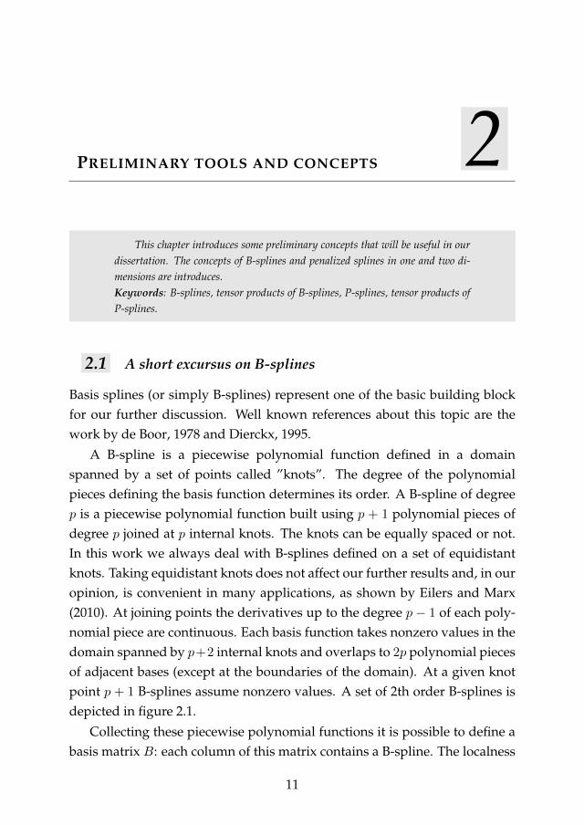
A B-spline is a piecewise polynomial function defined in a domainspanned by a set of points called ”knots”. The degree of the polynomialpieces defining the basis function determines its order. A B-spline of degreep is a piecewise polynomial function built using p + 1 polynomial pieces ofdegree p joined at p internal knots. The knots can be equally spaced or not.In this work we always deal with B-splines defined on a set of equidistantknots. Taking equidistant knots does not affect our further results and, in ouropinion, is convenient in many applications, as shown by Eilers and Marx(2010). At joining points the derivatives up to the degree p − 1 of each poly-nomial piece are continuous. Each basis function takes nonzero values in thedomain spanned by p+2 internal knots and overlaps to 2p polynomial piecesof adjacent bases (except at the boundaries of the domain). At a given knotpoint p + 1 B-splines assume nonzero values. A set of 2th order B-splines isdepicted in figure 2.1.
Collecting these piecewise polynomial functions it is possible to define abasis matrix B: each column of this matrix contains a B-spline. The localness
11
12 Chapter 2. Preliminary tools and concepts
0.0 0.2 0.4 0.6 0.8 1.0
0.0
0.2
0.4
0.6
0.8
x
0.0 0.2 0.4 0.6 0.8 1.0
0.0
0.2
0.4
0.6
0.8
Figure 2.1: One 3th order B-spline with its polynomial components. The second panelshown five 3th order B-splines.
of the polynomials defining the bases makes the B matrix really sparse sothat each of its row contains only few nonzero elements. This sparseness is animportant feature making B-splines computationally convenient for functioninterpolation and approximation.
B =
B1(x1) B2(x1) B3(x1) ... Bn(x1)
B1(x2) B2(x2) B3(x2) ... Bn(x2)...
......
......
B1(xn) B2(xn) B3(xn) ... Bn(xn)
.
Several algorithms can be adopted to compute the basis spline functionsforming the B matrix. A not convenient way is to evaluate the polynomialsegments forming the basis functions analytically. A more practical approachis represented by the algorithm proposed by de Boor, 1978. The last alterna-tive that can be mentioned consists in computing the spline functions using

2.1. A short excursus on B-splines 13
differences between truncated power functions (Schumaker, 1981; Eilers andMarx, 2010).
The B-spline matrix B can be used to interpolate or approximate any un-known function. Suppose that we want to approximate the values y assumedby an unknown function f(x) for some values of x. If we denote withBj(x, p)the value of the jth B-spline at point x we can represent y using a linear com-bination of B-splines y(x) =
∑j cjBj(x, p) where cj is the jth B-spline coeffi-
cient.As shown by de Boor (1978), there is a convenient relationship between
the dth derivative of a B-spline of order p and a B-spline of reduced orderp − d. Indeed, if h is the distance between two adjacent knots, the followingrelation holds:
y(d) =∑j
cjB(d)j (x, p) =
∑j ∆(d)cjBj(x, p− d)
hd, (2.1)
where ∆(d)cj is a dth order difference operator applied to the B-spline coeffi-cients. So, if we define the dth order difference matrix D(d) the dth derivativebasis matrix can be defined as:
B(d)(x, p) =B(x, p− d) D(d)
hd.
A useful issue of B-splines is their direct generalizability to higher di-mensions. Higher dimensional basis matrices can be computed using tensorproducts of one dimensional B-splines.
Consider a x, y grid of values. If we define the B-splines Bx and By,the two-dimensional basis matrix is obtained as Kronecker product betweenthem:
Bxy = Bx ⊗By.
This formulation is valid only for x, y values defined on a regular grid. Inthe opposite case the two-dimensional basis matrix can be built using row-wise tensor products Bxy = (Bx ⊗ 1TL) (1TK ⊗By).
In analogy with the unidimensional case it is possible to exploit a usefulrelationship to compute partial derivatives basis splines:
∂p+qBxy∂xpyq
=∑i
∑j
cijB(p)i,xB
(q)j,y , (2.2)
14 Chapter 2. Preliminary tools and concepts
x
0.00.5
1.0
1.5
2.0
y
0.00.5
1.0
1.5
2.0
z
0.0
0.1
0.2
0.3
0.4
Figure 2.2: A tensor product B Spline.
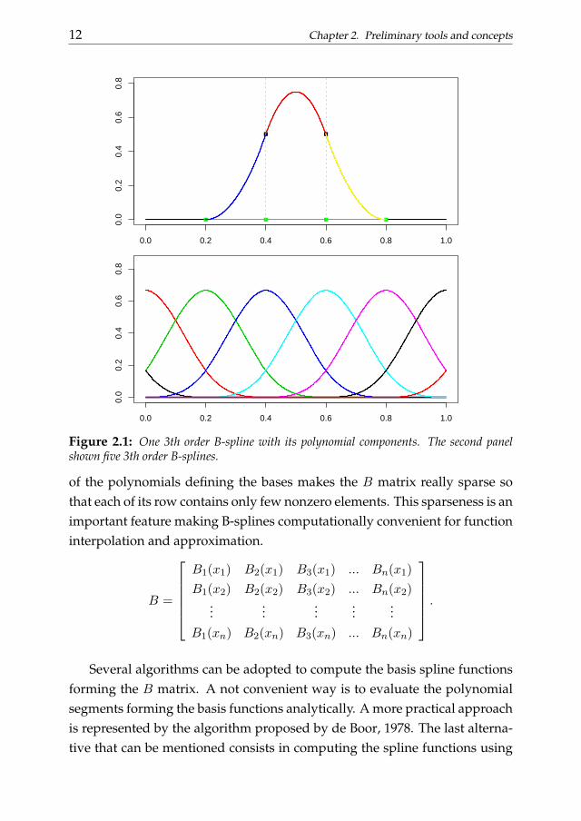
where B(p)x and B(q)
y represent the pth and qth order derivatives of Bx and Byrespectively. Figure 2.2 shows a single tensor product B-spline.
2.2 Penalized splines
P-splines have been introduced by Eilers and Marx (1996) as flexible smooth-ing procedures combining B-splines and difference penalties. Suppose that aset of data x, y, where x represents the independent (explanatory) vari-able and y the dependent variable, has been observed. We want to de-scribe y through an appropriate smooth function. Denote Bj(x; p) the valueof the jth B-spline of degree p defined on a domain spanned by equidis-tant knots (in case of not equally spaced knots our reasoning can be gen-eralized using divided differences). A curve that fits the data is given byy(x) =
∑nj=1 cjBj(x; q) where cj (with j = 1, ..., n) are the estimated B-splines
coefficients. Unfortunately this curve, obtained minimizing ‖y − Bc‖2 w.r.t.
2.2. Penalized splines 15
c, shows more variation than is justified by the data if the number of splinefunctions is too large. To avoid this overfitting tendency it is possible to es-timate c using a generous number of bases in a penalized regression frame-work:
c = argminc‖y −Bc‖2 + λ‖Dc‖2, (2.3)
where D is a dth order difference penalty matrix and λ is a smoothing pa-rameter. Second or third order difference penalties are suitable in many ap-plications. A second order difference matrix appears as follows:
D2 =
1 −2 1 0 0
0 1 −2 1 0
0 0 1 −2 1
.The optimal spline coefficients follow from (2.3) as:
c = (BTB + λDTD)−1BT y. (2.4)
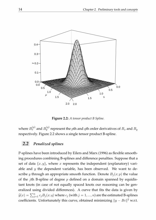
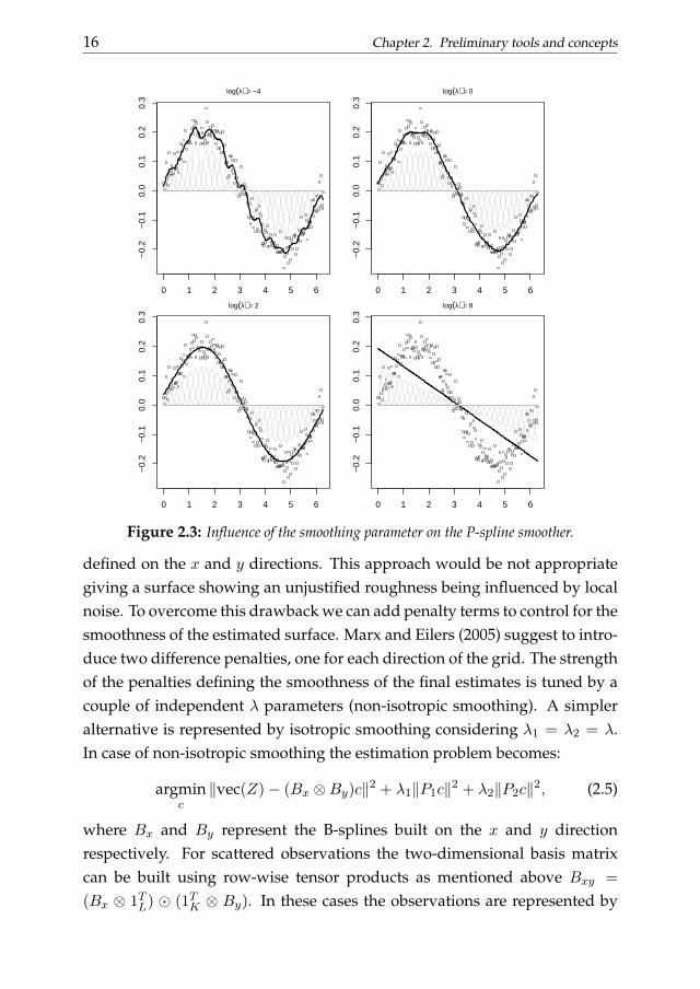
The smoothing parameter λ controls the trade-off between smoothnessand goodness of fit. For λ →∞ the final estimates tend to be constant whilefor λ → 0 the smoother tends to interpolate the observations. Figure 2.3shows how different values of the smoothing parameter influence the esti-mated smoother (for brevity only four λ values are shown). The data weresimulated by adding a Gaussian noise to a sine wave trend (200 observa-tions). The B-spline matrix has 30 equidistant knots. Cubic B-splines andsecond order difference penalties have been used to estimate the smoothingfunctions.
A P-spline smoother has some desirable properties. One of them is theconservation of moments. If we define vik = xki with integer k, the innerproduct yT vk defines the kth moment of y. A nice property of penalizedsplines built using a mth order difference penalty is that, for 0 < k < m, it istrue that yT vk = yT vk for each value of λ.
P-splines are easily generalizable to analyze multidimensional data. Sup-pose to have a dataset represented by a triplet x, y, Z where x and y in-dicate a grid of x, y values defining the domain over which the matrix Zhave been observed. Our aim is to efficiently summarize this 2D cloud ofpoints. To reach this purpose we could use a tensor product of B-splines
16 Chapter 2. Preliminary tools and concepts
0 1 2 3 4 5 6
−0.
2−
0.1
0.0
0.1
0.2
0.3
x
log(λ) = −4
0 1 2 3 4 5 6
−0.
2−
0.1
0.0
0.1
0.2
0.3
x
y
log(λ) = 0
0 1 2 3 4 5 6
−0.
2−
0.1
0.0
0.1
0.2
0.3
log(λ) = 2
0 1 2 3 4 5 6
−0.
2−
0.1
0.0
0.1
0.2
0.3
y
log(λ) = 8
Figure 2.3: Influence of the smoothing parameter on the P-spline smoother.
defined on the x and y directions. This approach would be not appropriategiving a surface showing an unjustified roughness being influenced by localnoise. To overcome this drawback we can add penalty terms to control for thesmoothness of the estimated surface. Marx and Eilers (2005) suggest to intro-duce two difference penalties, one for each direction of the grid. The strengthof the penalties defining the smoothness of the final estimates is tuned by acouple of independent λ parameters (non-isotropic smoothing). A simpleralternative is represented by isotropic smoothing considering λ1 = λ2 = λ.In case of non-isotropic smoothing the estimation problem becomes:
argminc‖vec(Z)− (Bx ⊗By)c‖2 + λ1‖P1c‖2 + λ2‖P2c‖2, (2.5)
where Bx and By represent the B-splines built on the x and y directionrespectively. For scattered observations the two-dimensional basis matrixcan be built using row-wise tensor products as mentioned above Bxy =
(Bx ⊗ 1TL) (1TK ⊗ By). In these cases the observations are represented by

2.2. Penalized splines 17
three x, y, z vectors of same length. The P1 and P2 penalty matrices aredefined as follows:
P1 =
1 0 0
0 1 0
0 0 1
⊗D(d)1
and
P2 = D(d)2 ⊗
1 0 0
0 1 0
0 0 1
,whereD(d)
1 andD(d)2 are two dth order difference matrices. LetBxy = Bx⊗By
(or Bxy = (Bx ⊗ 1TL) (1TK ⊗ By) if we observe scattered observations) thenthe solution of the minimization problem in (2.5) is the coefficient matrix:
c = (BTxyBxy + λ1P
T1 P1 + λ2P
T2 P2)−1BTvec(Z). (2.6)
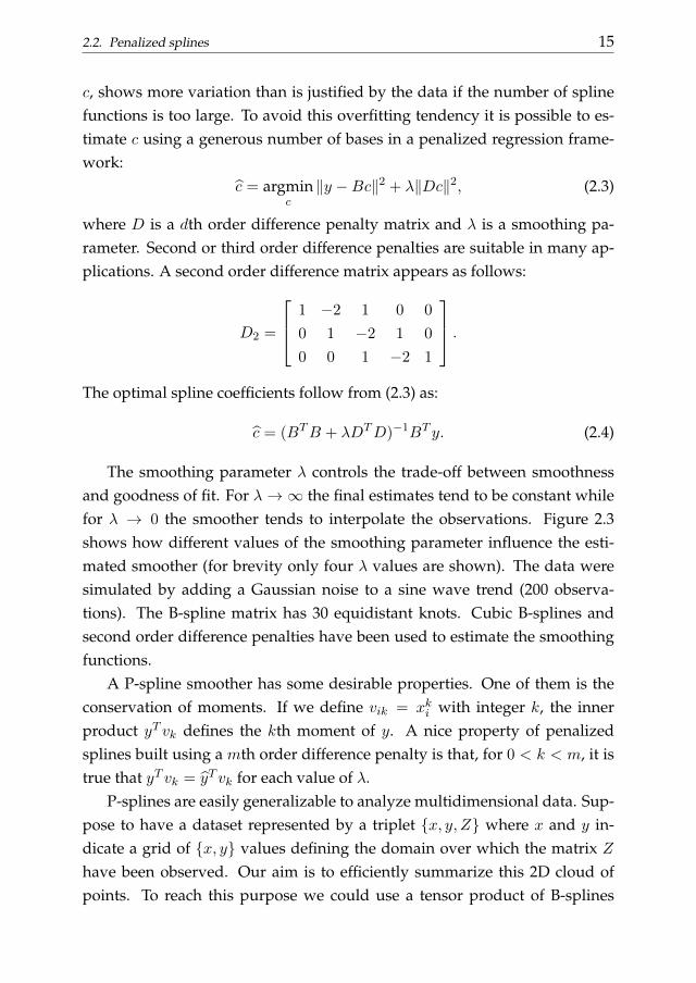
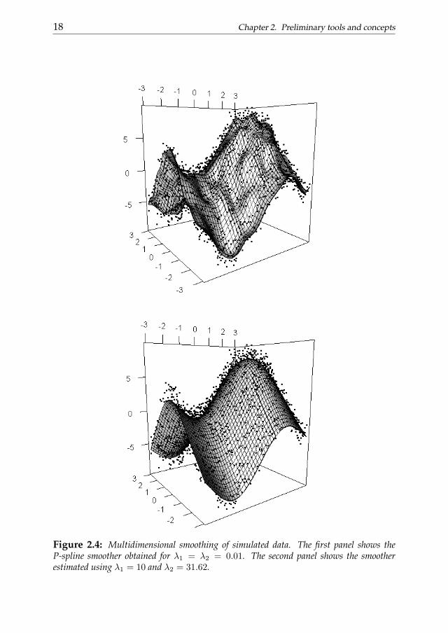
Figure2.4 shows a simulated non.isotropic two-dimensional P-splinesmoothing example. The computational effort needed to perform the esti-mates described above becomes quickly prohibitive as the number of obser-vations increases. An efficient algorithm (GLAM) has been proposed by Eil-ers et al. (2006). The cited algorithm have been used in every 2D applicationsdiscussed in this work.
18 Chapter 2. Preliminary tools and concepts
Figure 2.4: Multidimensional smoothing of simulated data. The first panel shows theP-spline smoother obtained for λ1 = λ2 = 0.01. The second panel shows the smootherestimated using λ1 = 10 and λ2 = 31.62.
THE L-CURVE FOR OPTIMAL SMOOTHING 3The L-curve, adopted for the selection of the regularization parame-
ter in ill-posed inverse problems, shows a parametric plot of the residualsvs the penalty. The corner of the L indicates the right amount of regu-larization. The L-curve is easy to compute and works surprisingly wellalso for smoothing data with correlated noise. We present the theoreticalbackground, an alternative criterion to find the corner automatically, andapplications to real data.Keywords: Whittaker and P-spline smoothers, L-curve, cross validation.
3.1 Introduction
Penalized regression has a prominent place in modern smoothing. It com-bines a rich set of basis functions with a roughness penalty, to tune smooth-ness of the estimated curve. B-splines are a popular choice for the basis func-tions, but others prefer truncated power functions. The penalty can be de-rived from classical roughness measures, like the integrated squared secondderivative, or it can be discrete, working directly on the regression coeffi-cients. An extensive discussion is presented by Eilers and Marx (2010).
P-splines (Eilers and Marx, 1996) combine a B-spline matrix with apenalty on (higher order) differences of their coefficients. If we have dataon equally spaced positions and go to the limit, we will have a basis functionfor each observation and the regression basis will be the identity matrix. Thisbrings us back to the Whittaker’s smoother (Whittaker, 1922; Eilers, 2003),which became popular in the econometric literature as the Hodrick-Prescottfilter (Hodrick and Prescott, 1997). It is an attractive smoother, because effec-tively the basis functions disappear and with just one smoothing parameterone can move all the way from a straight line fit to essentially reproducing
19

20 Chapter 3. The L-curve for optimal smoothing
the data themselves. On the other hand sparse matrix algorithms allow fastcomputations.
It is desirable to have an automatic procedure for selecting a value forthe smoothing parameter. In principle many choices are available. The moststraightforward ones are leave-one-out cross-validation (LOO-CV), general-ized cross-validation (Wahba, 1990) and AIC (Akaike’s Information Crite-rion) or BIC (Bayesian Information Criterion). It is also possible to exploitthe similarity between penalized regression and mixed models and then thesmoothing parameter becomes a ratio of variances (Schall, 1991; Ruppert,2003).
The established method for selection of the smoothing parameter havetwo things in common: 1) they require the computation of the effective modeldimension, and 2) they are sensitive to serial correlation in the noise aroundthe trend. The effective dimension is equal to the trace of the smoother ma-trix, and so inversion of a large matrix is required; for long data series thisis prohibitive. Serial correlation generally leads to under-smoothing. At firstsight this is surprising, but it is not hard to see why it happens. Indeed crossvalidation methods assume data with independent noise. If f(xk) is the esti-mated value taking into account the leave-out procedure yk is an observation:
E[(f(xk)− yk)2
]= E
[(f(xk)− f(xk))
2]
+ σ2 − 2Cov[f(xk), yk],
which shows that the expected squared error for a cross validation term isequal to the true expected squared error plus the noise variance σ2 minustwo times the covariance between the observed data and the estimates. Evenif this last term is not zero (as in the case of serial dependence in the noisecomponent) the cross validation misspecifies it to be equal to zero. (see Car-mack et al. (Carmack et al., 2012)). This leads to a smoothing function thattends to consider the correlated errors as a part of the wanted signal.
In this chapter we present and alternative approach, based on the L-curvemethod for ill-posed inverse problems (Hansen, 1992; Hansen and O’Leary,1993; Hansen, 2000). The L-curve is a plot of the logarithm of the magni-tude of the penalty term against the log of the sums of squares of the residu-als, parameterized by the regularization parameter λ. In the case of inverseproblems a very pronounced L-shape is obtained and a good value of theregularization parameter is found in its corner. As far as we know, the L-
3.1. Introduction 21
curve has not been used for smoothing, but it turns out to be very valuablethere. The shape is less pronounced that of an L, but a corner is present andit can easily be located numerically by following the path parameterized thesmoothing parameter λ.
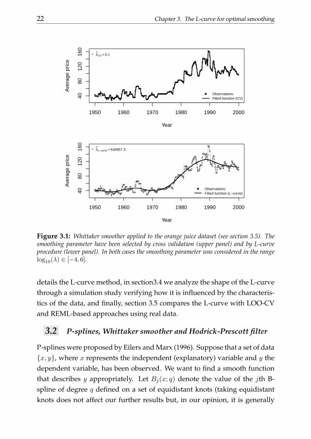
There is no need to compute the effective model dimension, so using theL-curve makes smoothing of long data series practical. And, very surpris-ingly, it is not affected by correlated noise as already noticed by Hansen forTikhonov regularization applications. This is illustrated in figure 3.1, show-ing historical data of the price of orange juice (Stock and Watson, 2003), withvery strong serial correlation. For the upper panel the amount of smoothingwas chosen automatically by LOO-CV, while for the lower panel the L-curvewas used. It is quite clear that no meaningful trend can be obtained withLOO-CV; GCV, AIC and the mixed model approach lead to very similar re-sults (not shown). On the other hand the trend in the lower panel of the figureappears to summarize the data well. We have no compelling explanations ofwhy the L-curve works so well.
Of course, the corner of an L-shaped curve is a special point, but it isnot clear why it marks a good choice of smoothing parameter. The relativechanges of both the penalty and the size of the residuals are small there, andapproximately equal, and apparently that matters. The insensitivity to serialcorrelation in the noise is also hard to explain but it is significant that theL-curve that does not rely on any statistical model. This method shows ex-cellent performance in practice, so we like to share our experiences with thestatistical community.
Krivobokova and Kauermann (2007) approach smoothing as a mixedmodel with correlated noise and present a REML estimation algorithm. Wecompare their results with those obtained using the L-curve and find thatthe latter performs better and faster (especially when complex covariancestructure are needed to describe the data). It is necessary to clarify that theevaluations about the computational efficiency of the methods discussed areobtained considering an high-level programming language such as R and us-ing its stand alone functions.
This chapter is organized as follows: in section 3.2 we introduce thesmoothing procedures that will be used in our discussion, together withsome standard smoothing selection procedures, section 3.3 describes in more
22 Chapter 3. The L-curve for optimal smoothing
1950 1960 1970 1980 1990 2000
4080
120
160
Year
Ave
rage
pric
e
ObservationsFitted function (CV)
* λCV = 0.1
1950 1960 1970 1980 1990 2000
4080
120
160
Year
Ave
rage
pric
e
ObservationsFitted function (L−curve)
* λL−curve = 630957.3
Figure 3.1: Whittaker smoother applied to the orange juice dataset (see section 3.5). Thesmoothing parameter have been selected by cross validation (upper panel) and by L-curveprocedure (lower panel). In both cases the smoothing parameter was considered in the rangelog10(λ) ∈ [−4, 6].
details the L-curve method, in section3.4 we analyze the shape of the L-curvethrough a simulation study verifying how it is influenced by the characteris-tics of the data, and finally, section 3.5 compares the L-curve with LOO-CVand REML-based approaches using real data.
3.2 P-splines, Whittaker smoother and Hodrick-Prescott filter
P-splines were proposed by Eilers and Marx (1996). Suppose that a set of datax, y, where x represents the independent (explanatory) variable and y thedependent variable, has been observed. We want to find a smooth functionthat describes y appropriately. Let Bj(x; q) denote the value of the jth B-spline of degree q defined on a set of equidistant knots (taking equidistantknots does not affect our further results but, in our opinion, it is generally
3.2. P-splines, Whittaker smoother and Hodrick-Prescott filter 23
a good idea, see Eilers and Marx, 2010). A curve that fits the data is givenby y(x) =
∑nj=1 zjBj(x; q) where zj (with j = 1, ..., n) are the estimated B-
splines coefficients. Unfortunately this curve, that is obtained minimizing‖y −Bz‖2 w.r.t. z, usually shows more variation than is justified by the data.to avoid this phenomenon it is possible to estimate z using a penalized linearregression approach:
z = argminz‖y −Bz‖2 + λ‖Dz‖2, (3.1)
where D is a mth order difference penalty matrix and λ is the smoothingparameter that controls the trade-off between smoothness and goodness offit. Solving (3.1) for the spline coefficients we get:
z = (BTB + λDTD)−1BT y. (3.2)
The Whittaker smoother (Whittaker, 1922) can be viewed as a special caseof the P-spline smoother. It arises when the observations are located on anequally-spaced grid, a knot is placed at each abscissa point, and B = I , theidentity matrix. In the econometric literature this smoother is also known asthe Hodrick-Prescott filter (Hodrick and Prescott, 1997). It was proposed byHodrick and Prescott as a tool to separate the cyclical component of a timeseries from raw data in order to obtain a smoothed version of the series. Thesmoothed time series has the advantage to be less influenced by short termfluctuations than by long term ones. In their paper Hodrick and Prescottsuggest a λ = 1600 as a good choice. Eilers (2003) uses a leave-one-out cress-validation. Kauermann et al. (2011), work in the other direction, replacingthe H-P filter with a penalized spline smoother.
Popular methods for smoothing parameter selection are: the Akaike In-formation Criterion, Cross Validation. AIC estimates the predictive log like-lihood, by correcting the log likelihood of the fitted model (Λ) by its effectivedimension (ED): AIC = 2ED − 2Λ. Following Hastie and Tibshirani (1990)we can compute the effective dimension as ED = tr[(BTB + λDTD)−1BTB]
for the P-spline smoother while ED = tr[(I + λDTD)−1] is the effective di-mension of the Whittaker smoother, and
2` = −2n ln σ2n∑i=1
(yi − yi)2
σ20
,
24 Chapter 3. The L-curve for optimal smoothing
where σ is the maximum likelihood estimate of σ. But σ2 =∑
i(yi − y2i )
2/n,so the second term of ` is a constant. Hence the AIC can be written as:
AIC(λ) = 2ED + 2n ln σ. (3.3)
The optimal parameter is the one that minimizes the value of AIC(λ). LOO-CV chooses the value of λ that minimizes:
CV (λ) =
n∑i=1
[yi − yi1− hii
]2
, (3.4)
where hii is the ith diagonal entry of H = B(BTB + λDTD)−1BT for P-splines or H = (I + λDTD)−1 in case of the Whittaker smoother. Analogousto CV is the generalized cross validation measure (Wahba, 1990):
GCV (λ) =n∑i=1
[yi − yin− ED
]2
, (3.5)
whereED = tr(H). In analogy with cross validation we select the smoothingparameter that minimizes GCV (λ).
Related to this last method is the Generalize Correlated Cross Validationprocedure proposed by Carmack et al. This method exploits the possibilityto modify the definition of the degrees of freedom to be taken into accountin computing the GCV including the (estimated or a priori known) correla-tion structure in the noise component. If we denote with C this correlationmatrix and with S the smoothing matrix this modified GCV approach can becomputed as follows:
GCCV (λ) =
n∑i=1
1
n
[yi − yi
1− tr[2SC − SCST ]
]2
. (3.6)
3.3 L-curve selection method
The L-curve is a parameterized curve showing the two ingredients of everyregularization or smoothing procedure: the goodness of fit and the rough-ness of the final estimate. This approach was originally proposed by Hansen(1992) for the selection of the regularization parameter in ill-posed inverseproblems. Regularization arises both in statistics and inverse problems ap-plications even if the aim of the latter is slightly different. Indeed, in statis-tical modeling one posits a true data generating model and aims to estimate
3.3. L-curve selection method 25
it, in inverse problems one simply look for a ’good’ approximate solution ofa given equation without taking into account any data generating process.Also the errors are considered differently. An important parameter for thesolution of inverse problems is the error upper bound level while in statis-tical applications the error it treated as an exogenous component (see Vogel,1996).
In this section we study its applicability to statistical models and in par-ticular we focus on smoothing applications.
3.3.1 The L-curve in ridge regression
Ridge regression is a common regularization tool in statistics. It adds apenalty term to the standard regression problem to shrink the coefficients:
argminβ
‖y −Xβ‖2 + λ‖β‖2
β = (XTX + λI)−1XT y. (3.7)
The strength of the shrinkage depends on λ. Define:
ω(λ); θ(λ) = ‖y −Xβ‖2; ‖β‖2 and ψ(λ);φ(λ) = log(ω); log(θ).
The L-curve is a plot of φ(λ) vs. ψ(λ), parameterized by λ. the name.Figure 3.2 shows a toy example. A sample of 200 realizations of 50 ex-
planatory variables was drawn from a multivariate normal distribution withmean vector µi = 1 with high correlation (ρ ∈ 0.7, 0.8, 0.9, 0.99). The de-pendent variable was obtained as a linear combination of the 50 independentvariables plus a random noise yi = cX +N(0, 0.2) (where cj is the regressionparameter associated to each independent variable randomly drawn from auniform distribution). The shape of the curve is true to its name. It shows acorner in a region characterized by intermediate values of ψ, φ and λ. Hansensuggested to select the regularization parameter that corresponds to the cor-ner, the point of maximum curvature. The curvature can be computed using:
k(λ) =ψ′φ′′ − ψ′′φ′
[(ψ′)2 + (φ′)2]3/2. (3.8)
The maximization of k(λ) requires the computation of the first and secondderivatives but the computations can be simplified in some cases as will be

26 Chapter 3. The L-curve for optimal smoothing
2.5 3.5 4.5 5.5
−0.
50.
51.
52.
5
ρ = 0.7
ψ = log(∑(yi − zi)2)
φ=
log(
∑(z
i)2 )
00.5 1
3.25
5
4.5
4
* log(λ) = 3.25
2.5 3.5 4.5 5.5
−0.
50.
51.
52.
5
ρ = 0.8
ψ = log(∑(yi − zi)2)
φ=
log(
∑(z
i)2 )
00.51
3
5
4.5
4
* log(λ) = 3
2.5 3.5 4.5 5.5
−0.
50.
51.
52.
5
ρ = 0.9
ψ = log(∑(yi − zi)2)
φ=
log(
∑(z
i)2 )
00.51
2.75
5
4.5
4
* log(λ) = 2.75
2.5 3.5 4.5 5.5
−0.
50.
51.
52.
5
ρ = 0.99
ψ = log(∑(yi − zi)2)
φ=
log(
∑(z
i)2 )
0
0.5
1
2
5
4.5
4
* log(λ) = 2
Figure 3.2: Four L-curves obtained for simulated ridge regression examples with differ-ent degrees of correlation between the explanatory variables. The corner point representsthe point of maximum curvature while the other points represent the points used to drawthe curve. For some points the associated logarithmic value of the parameter is shown(log10(λ) ∈ [0, 5]).
shown in what follows. It is important to notice that that while methods suchas cross validation optimize the smoothing parameter minimizing a measureof the prevision accuracy, the L-curve suggests to look for the λ parameterthat guarantees an optimal compromise between the residual sum of squaresand the amount of penalty.
The L-curve is usually characterized by two components: a vertical andan horizontal part (consider the fourth panel of figure 3.2). The vertical partis drawn for small values of the regularization parameter. In this region theresidual sum of squares is small while the amount of penalty tends to be high.The second component is the horizontal one: it is drawn for increasing valuesof the smoothing parameter leading to higher residual sum of squares. This
3.3. L-curve selection method 27
flat part of the curve is characterized by a rather constant amount of penalty.If we think about an ideal L plot we can say that for a constant amount ofpenalty we could tune the residual sum of squares along the horizontal partof the plot. It is an ideal situation but it holds till we reach the corner of theL. At the corner we obtain the best goodness of fit for the smallest possibleprice (smallest penalty).
3.3.2 The L-curve in penalized smoothing
In section 3.2 we briefly introduced the P-spline and the Whittakersmoothers. Consider a P-spline smoother. Taking z = Bα, the followingquantities can be defined:
ω(λ); θ(λ) = ‖y −Bz‖2; ‖Dz‖2,
and the L-curve is given by:
L = ψ(λ);φ(λ) = log(ω); log(θ). (3.9)
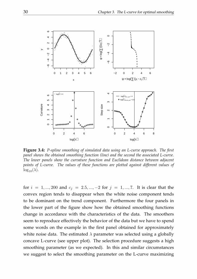
The L-curve for a simple smoothing problem is depicted in figure 3.4.These results were obtained from 200 observations simulated using the fol-lowing scheme: y = 5 sin(x) +N(0, 0.5) where x ∈ [0, 2π].
The lower panel of figure 3.4 shows the pointwise curvature function andthe Euclidean distance between adjacent points of the L-curve of the upperpanel. We notice that the smoothing parameters selected maximizing thecurvature and minimizing the Euclidean distance between adjacent pointsare the same. To understand why it is the case we can look at the L-curveclosely (see figure 3.2 or the second panel of figure 3.4). The density of thepoints defining the curve tends to increase moving from the tail to the cornerof the L. We can exploit this characteristic to simplify the selection procedure.
3.3.3 A new selection criterion
The curvature function can be computed using (3.8) per each λ parameter ona given grid. If we set ` = log(λ), the rate of change of the arc length distancebetween each point on the curve w.r.t. ` is given by:
ds
d`=
√(dψ
d`
)2
+
(dφ
d`
)2
. (3.10)
28 Chapter 3. The L-curve for optimal smoothing
Minimizing it we obtain a good approximation of maxk(λ) when the L-curve shows a clear convex area (i.e. when there is a corner). This means thatwe can simplify the selection procedure. The corner, if it exists, coincides (atleast approximately) with the point satisfying:
min√
(∆ψ)2 + (∆φ)2. (3.11)
The criterion in (3.11) suggests that the best smoothing parameter can beselected minimizing the Euclidean distance between adjacent points on theL-curve. The Euclidean distance between these points describes a U-shapedas shown in the last panel of figure 3.4. Shahrak (2013) already coined thename U-curve, although with a different definition. To avoid confusion, wechristened our procedure the ”V-curve”.
It is possible to use a more precise criterion based on an algorithm tocompute the gradient ∇`i(L) on a really fine grid of smoothing parameter.Indeed, using the well known equation for the computation of the B-splinesderivatives (de Boor, 1978), we can look for the λ satisfying (3.11) on a finegrid of candidate parameters. The optimal smoothing parameter is then theλ on the this grid that minimizes the magnitude of the gradient.
First of all we can approximate the functions ψ and φ using basis func-tions. If we define the matrix L = [ψ φ]T , we can estimate a matrix of suitableB-spline coefficients as follows:
C =(BTB + kDTD
)−1BTL, (3.12)
where, in analogy with what we already discussed in the previous sections,Bis a B-spline basis matrix,D is a difference penalty matrix and we introduce areally small regularization parameter k (for instance k = 10−6) to ensure thewell-poseness of the problem. Given the B-spline coefficients matrix C it ispossible to estimate the derivatives of ψ and φw.r.t. ` using a derivative basismatrix B(`, p). This matrix can be obtained not only considering the originalgrid but also on a finer one. Indeed, in order to obtain B(`, p), we need to setonly the extreme values for ` being possible to make the grid as fine as weprefer.
The final estimates of the derivatives are the matrix G = BC. The rowsof this matrix represent the gradient of the L-curve for each value of `: G =
3.4. The shape of the L-curve 29
0 2 4 6 8
01
23
4
log(λ)
ψ⋅φ⋅
Wood surface: squared gradient components
0 2 4 6 8
12
34
log(λ)
* log(λ) = 6.7
Wood surface: squared gradient
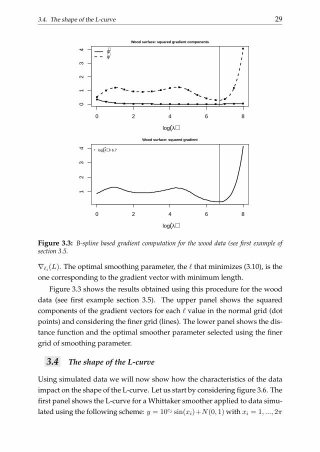
Figure 3.3: B-spline based gradient computation for the wood data (see first example ofsection 3.5.
∇`i(L). The optimal smoothing parameter, the ` that minimizes (3.10), is theone corresponding to the gradient vector with minimum length.
Figure 3.3 shows the results obtained using this procedure for the wooddata (see first example section 3.5). The upper panel shows the squaredcomponents of the gradient vectors for each ` value in the normal grid (dotpoints) and considering the finer grid (lines). The lower panel shows the dis-tance function and the optimal smoother parameter selected using the finergrid of smoothing parameter.
3.4 The shape of the L-curve
Using simulated data we will now show how the characteristics of the dataimpact on the shape of the L-curve. Let us start by considering figure 3.6. Thefirst panel shows the L-curve for a Whittaker smoother applied to data simu-lated using the following scheme: y = 10cj sin(xi)+N(0, 1) with xi = 1, ..., 2π
30 Chapter 3. The L-curve for optimal smoothing
0 1 2 3 4 5 6
−6
−4
−2
02
46
x
y
−2 0 2 4 6
−6
−4
−2
0
ψ = log(∑(yi − z1)2)
φ=
log(
∑(D
z i)2 )
0 2 4 6
01
23
45
6
log(λ)
Cur
vatu
re
* log(λ) = 4
0 2 4 6 8
01
23
4
log(λ)
Ste
p si
ze
log(λ)finer_grid = 4
log(λ)normal_grid = 3.9
Figure 3.4: P-spline smoothing of simulated data using an L-curve approach. The firstpanel shows the obtained smoothing function (line) and the second the associated L-curve.The lower panels show the curvature function and Euclidean distance between adjacentpoints of L-curve. The values of these functions are plotted against different values oflog10(λ).
for i = 1, ..., 200 and cj = 2.5, ...,−2 for j = 1, ..., 7. It is clear that theconvex region tends to disappear when the white noise component tendsto be dominant on the trend component. Furthermore the four panels inthe lower part of the figure show how the obtained smoothing functionschange in accordance with the characteristics of the data. The smoothersseem to reproduce effectively the behavior of the data but we have to spendsome words on the example in the first panel obtained for approximatelywhite noise data. The estimated λ parameter was selected using a globallyconcave L-curve (see upper plot). The selection procedure suggests a highsmoothing parameter (as we expected). In this and similar circumstanceswe suggest to select the smoothing parameter on the L-curve maximizing

3.4. The shape of the L-curve 31
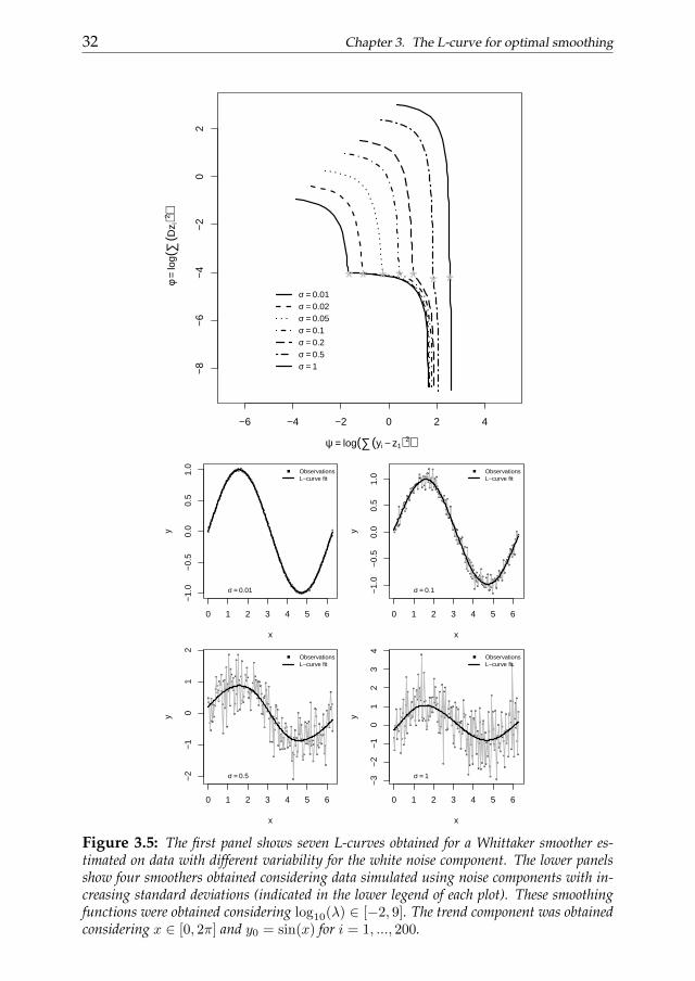
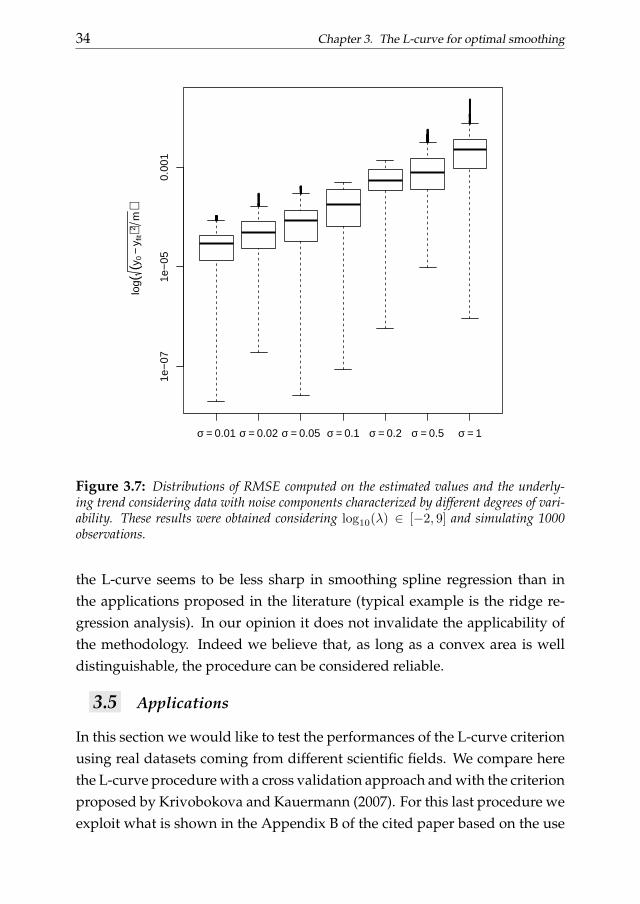
the curvature function. Indeed, even if the results cannot be considered reli-able because there is not a clear convex region on the L-curve, the curvatureselection criterion suggests a regularization parameter as large as possiblecorresponding to an area of the curve with a curvature as close as possi-ble to be positive. Also the characteristics of the error component influencethe shape of the L-curve. First of all the the variability of the white noisecomponent plays a role. Figure 3.5 shows that higher the variability is, lesssharp the L-curve appears. These results where obtained using 200 obser-vation simulated as follows: y = sin(x) + N(0, σj) with x = 1, ..., 2π andσj ∈ 0.01, 0.02, 0.05, 0.1, 0.2, 0.5, 1. All the smoothing functions shown inthe lower panels seem to efficiently catch the behavior of the data. Figure 3.7reproduces the distributions of residual mean square errors computed com-paring the fitted values and the underlying trend component consideringdata with random noise showing different standard deviations (we consid-ered now 1000 simulated observations). As we can notice the mean devia-tions for each variability level is close to zero even if those with a less variablenoise are smaller.
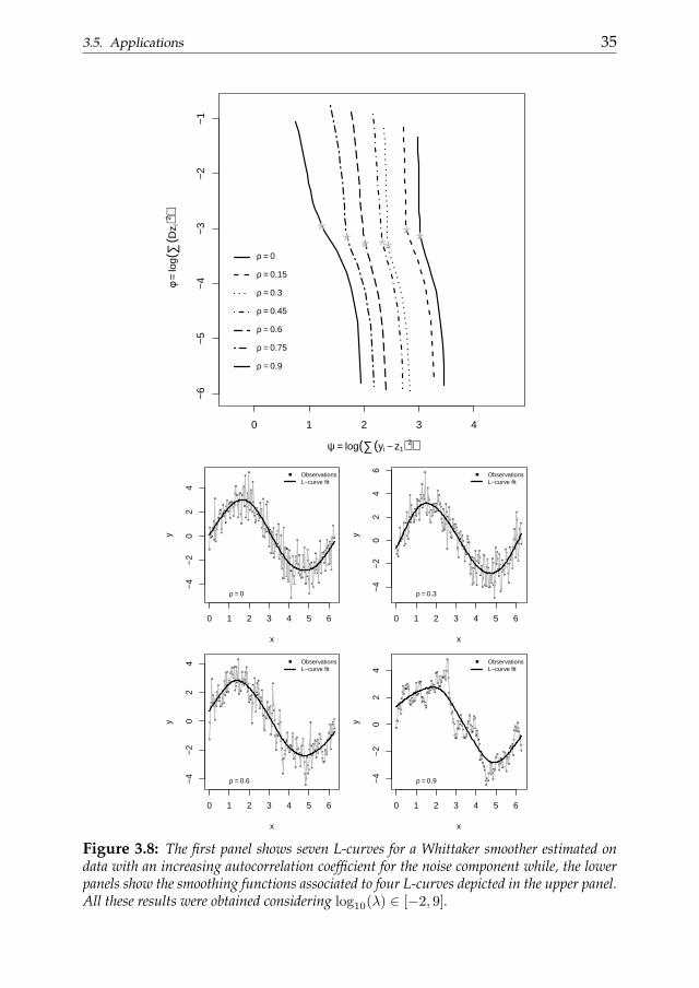
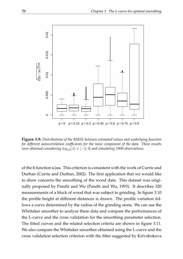
The L-curve turns out to be particularly useful when smoothing datawith autocorrelated noise. However the shape of the curve depends on thestrength of the serial correlation of the error component. Figure 3.8 showssome results obtained using the Whittaker smoother on a set of data sim-ulated as follows: y = 3 sin(xi) + AR(1, ρj , σ = 1) with xi = 1, ..., 2π fori = 1, ..., 200 and ρj = 0, ..., 0.9 for j = 1, ..., 7 where ρ indicates the auto-correlation coefficient. Slightly autocorrelated noise produces really sharpL-curves while higher degrees of serial correlation reduce the sharpness. Inany case the curves show clear convex areas. The lower part of figure 3.8shows some smoothing functions associated to some of the L-curves plottedin the upper part. It is possible to appreciate how well they reproduce the un-derlying data behavior in each scenario. Furthermore figure 3.9 summarizesthe performances obtained using a larger set of data (1000 observations) sim-ulated as before. It shows the distributions of the scaled squared deviationsof the estimated smoothing functions from the underlying trend componentfor each simulation setting. The mean deviations are all close to zero evenif the variability of the distributions seem to be influenced by the autocor-relation of the noise. In addition to these considerations we found also that
32 Chapter 3. The L-curve for optimal smoothing
−6 −4 −2 0 2 4
−8
−6
−4
−2
02
ψ = log(∑(yi − z1)2)
φ=
log(
∑(D
z i)2 )
*σ = 0.01
*σ = 0.02
*
σ = 0.05
*
σ = 0.1
*
σ = 0.2
*
σ = 0.5
*
σ = 1
0 1 2 3 4 5 6
−1.
0−
0.5
0.0
0.5
1.0
x
y
ObservationsL−curve fit
σ = 0.01
0 1 2 3 4 5 6
−1.
0−
0.5
0.0
0.5
1.0
x
y
ObservationsL−curve fit
σ = 0.1
0 1 2 3 4 5 6
−2
−1
01
2
x
y
ObservationsL−curve fit
σ = 0.5
0 1 2 3 4 5 6
−3
−2
−1
01
23
4
x
y
ObservationsL−curve fit
σ = 1
Figure 3.5: The first panel shows seven L-curves obtained for a Whittaker smoother es-timated on data with different variability for the white noise component. The lower panelsshow four smoothers obtained considering data simulated using noise components with in-creasing standard deviations (indicated in the lower legend of each plot). These smoothingfunctions were obtained considering log10(λ) ∈ [−2, 9]. The trend component was obtainedconsidering x ∈ [0, 2π] and y0 = sin(x) for i = 1, ..., 200.

3.4. The shape of the L-curve 33
−4 −2 0 2 4 6
−8
−6
−4
−2
02
ψ = log(∑(yi − z1)2)
φ=
log(
∑(D
z i)2 )
*
c1 = 0.01
*
c2 = 0.1
*
c3 = 1
*c4 = 5*
c5 = 10
*
c6 = 50
*
c7 = 100
0 1 2 3 4 5 6
−4
−3
−2
−1
01
23
x
y
ObservationsL−curve fit
c = 0.01
0 1 2 3 4 5 6
−3
−2
−1
01
23
x
y
ObservationsL−curve fit
c = 1
0 1 2 3 4 5 6
−10
−5
05
10
x
y
ObservationsL−curve fit
c = 10
0 1 2 3 4 5 6
−10
0−
500
5010
0
x
y
ObservationsL−curve fit
c = 100
Figure 3.6: The first panel shows seven L-curves obtained for a Whittaker smoother es-timated on data with different weights for the signal component while, the lower panelsshow four smoothers obtained considering data simulated using different weights for the thiscomponent (indicated in the lower legend of each plot). All these results were obtained con-sidering log10(λ) ∈ [0, 9].
34 Chapter 3. The L-curve for optimal smoothing
log(
(y0
−y f
it)2m
)
σ = 0.01 σ = 0.02 σ = 0.05 σ = 0.1 σ = 0.2 σ = 0.5 σ = 1
1e−
071e
−05
0.00
1
Figure 3.7: Distributions of RMSE computed on the estimated values and the underly-ing trend considering data with noise components characterized by different degrees of vari-ability. These results were obtained considering log10(λ) ∈ [−2, 9] and simulating 1000observations.
the L-curve seems to be less sharp in smoothing spline regression than inthe applications proposed in the literature (typical example is the ridge re-gression analysis). In our opinion it does not invalidate the applicability ofthe methodology. Indeed we believe that, as long as a convex area is welldistinguishable, the procedure can be considered reliable.
3.5 Applications
In this section we would like to test the performances of the L-curve criterionusing real datasets coming from different scientific fields. We compare herethe L-curve procedure with a cross validation approach and with the criterionproposed by Krivobokova and Kauermann (2007). For this last procedure weexploit what is shown in the Appendix B of the cited paper based on the use
3.5. Applications 35
0 1 2 3 4
−6
−5
−4
−3
−2
−1
ψ = log(∑(yi − z1)2)
φ=
log(
∑(D
z i)2 )
*ρ = 0
*
ρ = 0.15
*
ρ = 0.3
*
ρ = 0.45
*
ρ = 0.6
*
ρ = 0.75
*
ρ = 0.9
0 1 2 3 4 5 6
−4
−2
02
4
x
y
ObservationsL−curve fit
ρ = 0
0 1 2 3 4 5 6
−4
−2
02
46
x
y
ObservationsL−curve fit
ρ = 0.3
0 1 2 3 4 5 6
−4
−2
02
4
x
y
ObservationsL−curve fit
ρ = 0.6
0 1 2 3 4 5 6
−4
−2
02
4
x
y
ObservationsL−curve fit
ρ = 0.9
Figure 3.8: The first panel shows seven L-curves for a Whittaker smoother estimated ondata with an increasing autocorrelation coefficient for the noise component while, the lowerpanels show the smoothing functions associated to four L-curves depicted in the upper panel.All these results were obtained considering log10(λ) ∈ [−2, 9].
36 Chapter 3. The L-curve for optimal smoothing
(y0
−y f
it)2m
ρ = 0 ρ = 0.15 ρ = 0.3 ρ = 0.45 ρ = 0.6 ρ = 0.75 ρ = 0.9
00.
005
0.01
0.01
50.
02
Figure 3.9: Distributions of the RMSE between estimated values and underlying functionfor different autocorrelation coefficients for the noise component of the data. These resultswere obtained considering log10(λ) ∈ [−2, 9] and simulating 1000 observations.
of the R function nlme. This criterion is consistent with the work of Currie andDurban (Currie and Durban, 2002). The first application that we would liketo show concerns the smoothing of the wood data. This dataset was origi-nally proposed by Pandit and Wu (Pandit and Wu, 1993). It describes 320measurements of a block of wood that was subject to grinding. In figure 3.10the profile height at different distances is drawn. The profile variation fol-lows a curve determined by the radius of the grinding stone. We can use theWhittaker smoother to analyze these data and compare the performances ofthe L-curve and the cross validation for the smoothing parameter selection.The fitted curves and the related selection criteria are shown in figure 3.11.We also compare the Whittaker smoother obtained using the L-curve and thecross validation selection criterion with the filter suggested by Krivobokova
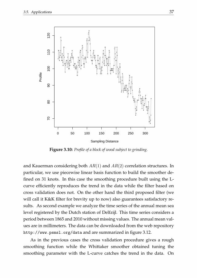
3.5. Applications 37
0 50 100 150 200 250 300
7080
9010
011
012
0
Sampling Distance
Pro
file
Figure 3.10: Profile of a block of wood subject to grinding.
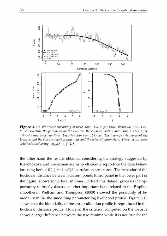
and Kauerman considering both AR(1) and AR(2) correlation structures. Inparticular, we use piecewise linear basis function to build the smoother de-fined on 31 knots. In this case the smoothing procedure built using the L-curve efficiently reproduces the trend in the data while the filter based oncross validation does not. On the other hand the third proposed filter (wewill call it K&K filter for brevity up to now) also guarantees satisfactory re-sults. As second example we analyze the time series of the annual mean sealevel registered by the Dutch station of Delfzijl. This time series considers aperiod between 1865 and 2010 without missing values. The annual mean val-ues are in millimeters. The data can be downloaded from the web repositoryhttp://www.psmsl.org/data and are summarized in figure 3.12.
As in the previous cases the cross validation procedure gives a roughsmoothing function while the Whittaker smoother obtained tuning thesmoothing parameter with the L-curve catches the trend in the data. On
38 Chapter 3. The L-curve for optimal smoothing
0 50 100 150 200 250 300
7080
9010
012
0
Sampling Distance
Pro
file
ObservationsL−curve fitK&K filter AR1K&K filter AR2CV fit
−2 0 2 4 6 8
0.8
1.0
1.2
1.4
1.6
log(λ)
log(
CV
(λ))
* log(λ)CV = −1.4
−2 0 2 4 6
−4
−2
02
4
ψ
φ
* log(λ)L−curve = 6.4
Figure 3.11: Whittaker smoothing of wood data. The upper panel shows the results ob-tained selecting the parameter by the L-curve, the cross validation and using a K&K filterdefined using piecewise linear basis functions on 31 knots. The lower panels represent theL-curve and the cross validation functions and the selected parameters. These results wereobtained considering log10(λ) ∈ [−2, 8].
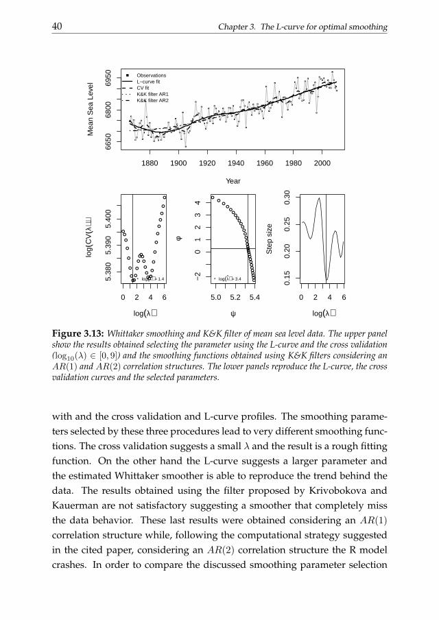
the other hand the results obtained considering the strategy suggested byKrivobokova and Kauerman seems to efficiently reproduce the data behav-ior using both AR(1) and AR(2) correlation structures. The behavior of theEuclidean distance between adjacent points (third panel in the lower part ofthe figure) shows some local minima. Indeed this dataset gives us the op-portunity to briefly discuss another important issue related to the P-splinesmoothers. Welham and Thompson (2009) showed the possibility of bi-modality in the the smoothing parameter log likelihood profile. Figure 3.13shows that the bimodality of the cross validation profile is reproduced in theEuclidean distance profile. However the criterion computed on the L-curveshows a large difference between the two minima while it is not true for the

3.5. Applications 39
1880 1900 1920 1940 1960 1980 2000
6650
6700
6750
6800
6850
6900
6950
Year
Mea
n se
a le
vel
Figure 3.12: Annual mean sea level registered in Delfzijl for the period 1865-2010.
cross validation criterion. The last example that we would like to discussis the orange juice price data already introduced in section 3.1. The originaldataset contains three time series: the average producer price for frozen or-ange juice, the producer price index for finished goods and the number offreezing degree days at the Orlando airport. The orange juice price serieswas divided by the overall Producer Price Index for finished goods to adjustfor general price inflation. As we did before, we will concentrate only onthe monthly series of the prices. From figure 3.1 it appeared clear that thisdataset represents a really hard smoothing exercise. We again compare theL-curve procedure with a cross validation approach and with the criterionproposed by Krivobokova and Kauerman. Following the cited paper we usepiecewise linear basis functions defined on 63 knots to build the smoother.In figure 3.14 the results obtained smoothing the orange juice prices time se-ries with a Whittaker smoother and the K&K procedure are shown together
40 Chapter 3. The L-curve for optimal smoothing
1880 1900 1920 1940 1960 1980 2000
6650
6800
6950
Year
Mea
n S
ea L
evel
ObservationsL−curve fitCV fitK&K filter AR1K&K filter AR2
0 2 4 6
5.38
05.
390
5.40
0
log(λ)
log(
CV
(λ))
* log(λ) = 1.4
5.0 5.2 5.4
−2
01
23
4
ψ
φ
* log(λ) = 3.4
0 2 4 6
0.15
0.20
0.25
0.30
log(λ)
Ste
p si
ze
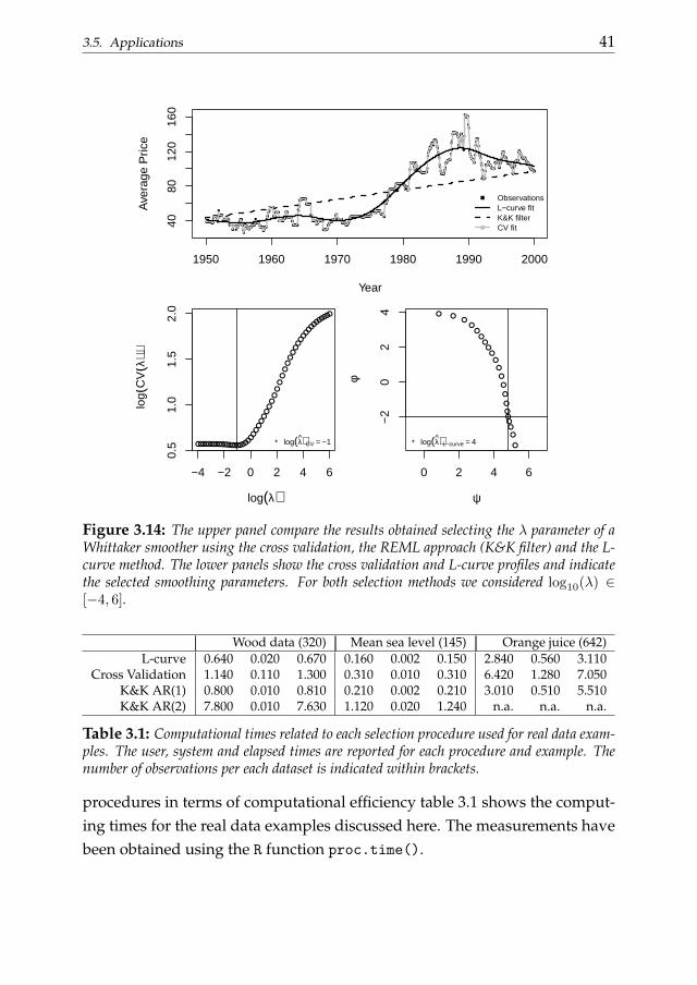
Figure 3.13: Whittaker smoothing and K&K filter of mean sea level data. The upper panelshow the results obtained selecting the parameter using the L-curve and the cross validation(log10(λ) ∈ [0, 9]) and the smoothing functions obtained using K&K filters considering anAR(1) and AR(2) correlation structures. The lower panels reproduce the L-curve, the crossvalidation curves and the selected parameters.
with and the cross validation and L-curve profiles. The smoothing parame-ters selected by these three procedures lead to very different smoothing func-tions. The cross validation suggests a small λ and the result is a rough fittingfunction. On the other hand the L-curve suggests a larger parameter andthe estimated Whittaker smoother is able to reproduce the trend behind thedata. The results obtained using the filter proposed by Krivobokova andKauerman are not satisfactory suggesting a smoother that completely missthe data behavior. These last results were obtained considering an AR(1)
correlation structure while, following the computational strategy suggestedin the cited paper, considering an AR(2) correlation structure the R modelcrashes. In order to compare the discussed smoothing parameter selection
3.5. Applications 41
1950 1960 1970 1980 1990 2000
4080
120
160
Year
Ave
rage
Pric
e
ObservationsL−curve fitK&K filterCV fit
−4 −2 0 2 4 6
0.5
1.0
1.5
2.0
log(λ)
log(
CV
(λ))
* log(λ)CV = −1
0 2 4 6
−2
02
4
ψ
φ
* log(λ)L−curve = 4
Figure 3.14: The upper panel compare the results obtained selecting the λ parameter of aWhittaker smoother using the cross validation, the REML approach (K&K filter) and the L-curve method. The lower panels show the cross validation and L-curve profiles and indicatethe selected smoothing parameters. For both selection methods we considered log10(λ) ∈[−4, 6].
Wood data (320) Mean sea level (145) Orange juice (642)L-curve 0.640 0.020 0.670 0.160 0.002 0.150 2.840 0.560 3.110
Cross Validation 1.140 0.110 1.300 0.310 0.010 0.310 6.420 1.280 7.050K&K AR(1) 0.800 0.010 0.810 0.210 0.002 0.210 3.010 0.510 5.510K&K AR(2) 7.800 0.010 7.630 1.120 0.020 1.240 n.a. n.a. n.a.
Table 3.1: Computational times related to each selection procedure used for real data exam-ples. The user, system and elapsed times are reported for each procedure and example. Thenumber of observations per each dataset is indicated within brackets.
procedures in terms of computational efficiency table 3.1 shows the comput-ing times for the real data examples discussed here. The measurements havebeen obtained using the R function proc.time().
42 Chapter 3. The L-curve for optimal smoothing
3.6 Conclusions
In this chapter we introduced an L-curve procedure for the selection of thesmoothing parameter in a P-splines framework. This approach selects thesmoothing parameter through a direct comparison between the goodnessof fit and the smoothness of the estimates. It was showed that the optimalsmoothing parameter can be selected by locating the point of maximum cur-vature, i.e. the corner, of the L-curve as was originally argued in the worksof Hansen (Hansen, 1992; Hansen and O’Leary, 1993). We also proposed analternative selection procedure based on the minimization of the Euclideandistance between the adjacent points of the curve: the V-curve criterion.
Using several simulation strategies it has been explained how the shapeof the L-curve is influenced by the underlying characteristics of the data andhow the selection procedure performs.
A comparison between the L-curve and the cross validation approacheswas examined using real data. It was highlighted that, selecting the smooth-ing parameter with a LOO-CV strategy, can suggest a too small λ parameterleading an under-smoothing of the data. This is true especially in the caseof data with a noise component showing serial correlation. In such cases,on the other hand, the L-curve procedure was found to be a robust selectionprocedure.
The same comparison was made to the strategy proposed byKrivobokova and Kauerman. It was found that the L-curve ensures resultsconsistent with those obtained using the K&K filter in two well behavedexamples over three. On the other hand it fails in a really extreme cases(i.e. the orange juice example). We also found that the L-curve procedureguarantees good results and a relatively lower computational effort in theanalysis of long data series.
Other REML-based approaches have been proposed in the literature.Currie and Durban (2002) also suggested to use a REML approach in order totake into account the correlation structure of the data. In their work the au-thors successfully analyzed the wood dataset modeling the correlation struc-ture through aAR(2) model showing results really close to what we obtainedin section 3.5. However we believe that our approach, besides being compu-tationally more convenient, guarantees good performances also in extreme
3.6. Conclusions 43
situations in which a suitable correlation structure is hard to define (such asthe orange juice price data).
From our discussion in this chapter appears also that the L-curve is a com-putationally efficient selection procedure if compared with standard proce-dures. Indeed it does not require the computation of the effective dimensionof the smoother at each step. In addition in some cases it is also possible tosimplify the selection procedure minimizing the Euclidean distance betweenadjacent points of the L-curve. This allows to avoid the computation of thefirst and second derivatives that appear in the curvature function. These fac-tors make this procedure computationally faster than those based on a leave-out or a mixed model framework. This is not a secondary feature especiallyin those cases in which the amount of data tends to increase the computa-tional cost of the entire statistical analysis.
It is necessary to underline that in some cases, the L-curve criterion couldnot lead to reliable results. It happens smoothing data that approach to apure white noise or when the signal component under the data tends to dis-appear. As shown in figure 3.15 and in the discussion of section 3.5 in thesecases the L-curve does not show a convex area and selecting the smooth-ing parameter through the minimization of the Euclidean distances leads tolight smoothing parameters. In these cases the curvature approach has to bepreferred because it tends to suggest a λ as close as possible to the optimalone. For this reason we recommend to use this procedure after a preliminary(also visual) inspection of the data. The L-curve procedure offers margins forfurther research. Indeed, in our opinion, it is not still clear why the cornercontains information about the optimal smoothing parameter and why it is arobust selection method in the case of data with correlated noise.
Furthermore we believe that the L-curve can also be generalized. Ourfuture research will concentrate on an L-curve criterion for multivariatesmoothing analyzes and on an L-curve based procedure suitable for expectilesmoothing problems.
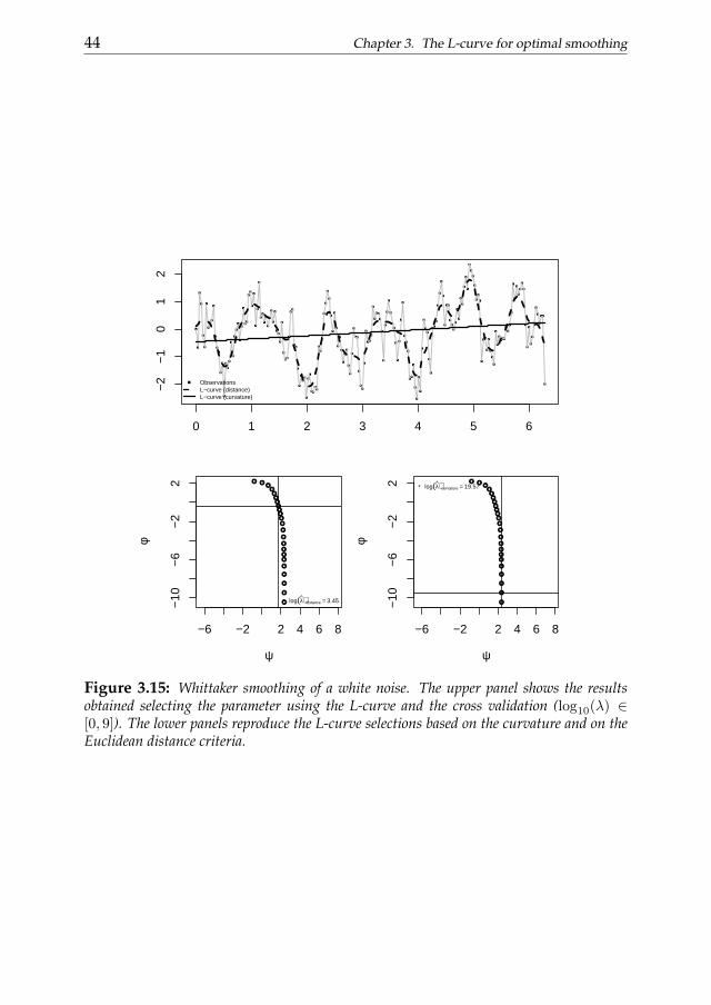
44 Chapter 3. The L-curve for optimal smoothing
0 1 2 3 4 5 6
−2
−1
01
2
x
y
ObservationsL−curve (distance)L−curve (curvature)
−6 −2 2 4 6 8
−10
−6
−2
2
ψ
φ
* log(λ)distance = 3.45
−6 −2 2 4 6 8
−10
−6
−2
2
ψ
φ
* log(λ)curvature = 19.57
Figure 3.15: Whittaker smoothing of a white noise. The upper panel shows the resultsobtained selecting the parameter using the L-curve and the cross validation (log10(λ) ∈[0, 9]). The lower panels reproduce the L-curve selections based on the curvature and on theEuclidean distance criteria.
THE L-SURFACE FOR NON-ISOTROPIC OPTI-MAL SMOOTHING 4
The L-surface is an attractive two-dimensional generalization of theL-curve procedure for optimal smoothing. However, one has to locate thepoint of maximal curvature of the surface, which is not easy. We introducea simplified procedure that replaces maximum curvature by a distance tobe minimized.Keywords: P-splines, L-curve, tensor products, penalties
4.1 Introduction
The L-curve criterion was proposed by Hansen (1992) and Hansen andO’Leary (1993) for selection of the regularization parameter in ill-conditionedinverse problems. In chapter 2 we have shown that it is an efficient and ro-bust method to select the penalty parameter in smoothing applications. TheL-curve does not require the computation of the effective model dimensionand is insensitive to correlated noise.
Here we discuss a generalization, the L-surface, for non-isotropic two-dimensional smoothing. It is a plot of the logarithm of the residual sum ofsquares against the logarithms of the sizes of the penalty terms, parameter-ized by the smoothing parameters. It appears as a surface with a nook and,in analogy with the L-curve, the optimal pair of smoothing parameters islocated in the deepest point of the nook. This is the point of maximum Gaus-sian curvature, as defined in differential geometry. Unfortunately, locatingthis point is a non-trivial computational task.
In the nook changes of parameters lead to small displacements on theL-surface. We compute the surface for a grid of values of the two smooth-ing parameters. Over this grid we search for the points on the surface thatare closest to each other. If we do this for the L-curve, in the case of one-
45
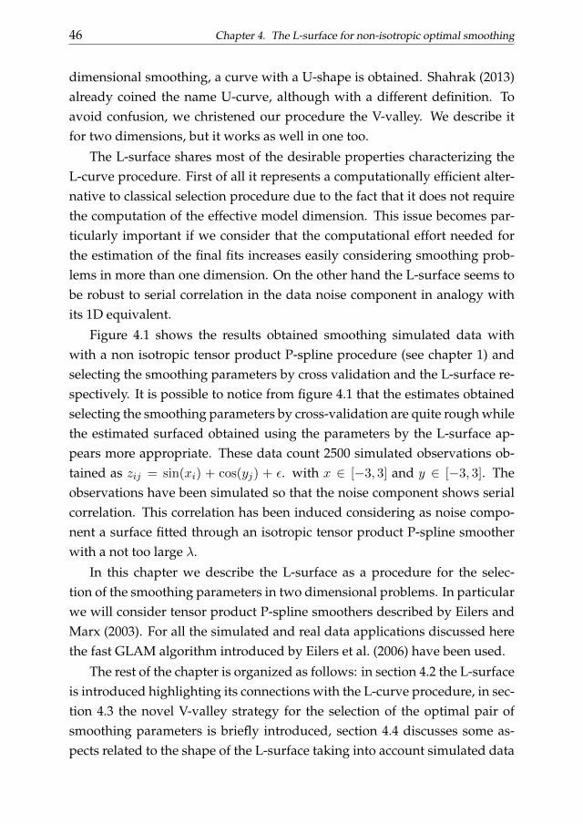
46 Chapter 4. The L-surface for non-isotropic optimal smoothing
dimensional smoothing, a curve with a U-shape is obtained. Shahrak (2013)already coined the name U-curve, although with a different definition. Toavoid confusion, we christened our procedure the V-valley. We describe itfor two dimensions, but it works as well in one too.
The L-surface shares most of the desirable properties characterizing theL-curve procedure. First of all it represents a computationally efficient alter-native to classical selection procedure due to the fact that it does not requirethe computation of the effective model dimension. This issue becomes par-ticularly important if we consider that the computational effort needed forthe estimation of the final fits increases easily considering smoothing prob-lems in more than one dimension. On the other hand the L-surface seems tobe robust to serial correlation in the data noise component in analogy withits 1D equivalent.
Figure 4.1 shows the results obtained smoothing simulated data withwith a non isotropic tensor product P-spline procedure (see chapter 1) andselecting the smoothing parameters by cross validation and the L-surface re-spectively. It is possible to notice from figure 4.1 that the estimates obtainedselecting the smoothing parameters by cross-validation are quite rough whilethe estimated surfaced obtained using the parameters by the L-surface ap-pears more appropriate. These data count 2500 simulated observations ob-tained as zij = sin(xi) + cos(yj) + ε. with x ∈ [−3, 3] and y ∈ [−3, 3]. Theobservations have been simulated so that the noise component shows serialcorrelation. This correlation has been induced considering as noise compo-nent a surface fitted through an isotropic tensor product P-spline smootherwith a not too large λ.
In this chapter we describe the L-surface as a procedure for the selec-tion of the smoothing parameters in two dimensional problems. In particularwe will consider tensor product P-spline smoothers described by Eilers andMarx (2003). For all the simulated and real data applications discussed herethe fast GLAM algorithm introduced by Eilers et al. (2006) have been used.
The rest of the chapter is organized as follows: in section 4.2 the L-surfaceis introduced highlighting its connections with the L-curve procedure, in sec-tion 4.3 the novel V-valley strategy for the selection of the optimal pair ofsmoothing parameters is briefly introduced, section 4.4 discusses some as-pects related to the shape of the L-surface taking into account simulated data

4.1. Introduction 47
Figure 4.1: Multidimensional smoothing of simulated data. The first panel shows a nonisotropic tensor product P-spline smoother obtained selecting the λ parameters by cross val-idation (λ1 = λ2 = 0.01). The second panel shows the smoother obtained selecting thetuning parameters through the L-surface procedure (λ1 = 10 and λ2 = 31.62).
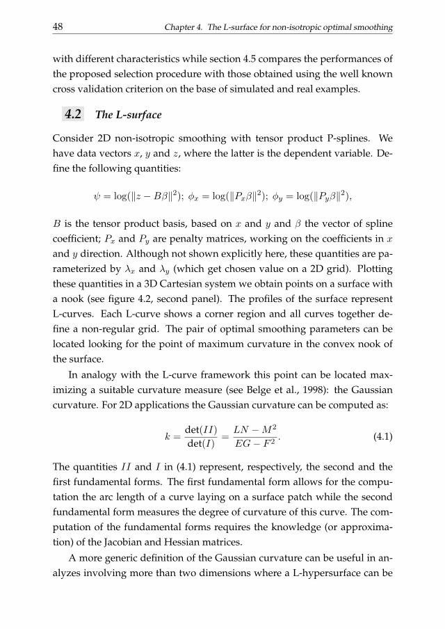
48 Chapter 4. The L-surface for non-isotropic optimal smoothing
with different characteristics while section 4.5 compares the performances ofthe proposed selection procedure with those obtained using the well knowncross validation criterion on the base of simulated and real examples.
4.2 The L-surface
Consider 2D non-isotropic smoothing with tensor product P-splines. Wehave data vectors x, y and z, where the latter is the dependent variable. De-fine the following quantities:
ψ = log(‖z −Bβ‖2); φx = log(‖Pxβ‖2); φy = log(‖Pyβ‖2),
B is the tensor product basis, based on x and y and β the vector of splinecoefficient; Px and Py are penalty matrices, working on the coefficients in x
and y direction. Although not shown explicitly here, these quantities are pa-rameterized by λx and λy (which get chosen value on a 2D grid). Plottingthese quantities in a 3D Cartesian system we obtain points on a surface witha nook (see figure 4.2, second panel). The profiles of the surface representL-curves. Each L-curve shows a corner region and all curves together de-fine a non-regular grid. The pair of optimal smoothing parameters can belocated looking for the point of maximum curvature in the convex nook ofthe surface.
In analogy with the L-curve framework this point can be located max-imizing a suitable curvature measure (see Belge et al., 1998): the Gaussiancurvature. For 2D applications the Gaussian curvature can be computed as:
k =det(II)
det(I)=LN −M2
EG− F 2. (4.1)
The quantities II and I in (4.1) represent, respectively, the second and thefirst fundamental forms. The first fundamental form allows for the compu-tation the arc length of a curve laying on a surface patch while the secondfundamental form measures the degree of curvature of this curve. The com-putation of the fundamental forms requires the knowledge (or approxima-tion) of the Jacobian and Hessian matrices.
A more generic definition of the Gaussian curvature can be useful in an-alyzes involving more than two dimensions where a L-hypersurface can be
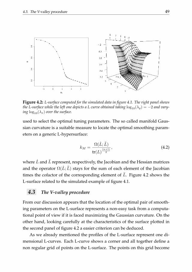
4.3. The V-valley procedure 49
−1 0 1 2 3
3.2
3.4
3.6
3.8
ψx
φ
Figure 4.2: L-surface computed for the simulated data in figure 4.1. The right panel showsthe L-surface while the left one depicts a L curve obtained taking log10(λy) = −2 and vary-ing log10(λx) over the surface.
used to select the optimal tuning parameters. The so called manifold Gaus-sian curvature is a suitable measure to locate the optimal smoothing param-eters on a generic L-hypersurface:
kM =Ω(L; L)
tr(L)(n+1)
2
, (4.2)
where L and L represent, respectively, the Jacobian and the Hessian matricesand the operator Ω(L; L) stays for the sum of each element of the Jacobiantimes the cofactor of the corresponding element of L. Figure 4.2 shows theL-surface related to the simulated example of figure 4.1.
4.3 The V-valley procedure
From our discussion appears that the location of the optimal pair of smooth-ing parameters on the L-surface represents a non-easy task from a computa-tional point of view if it is faced maximizing the Gaussian curvature. On theother hand, looking carefully at the characteristics of the surface plotted inthe second panel of figure 4.2 a easier criterion can be deduced.
As we already mentioned the profiles of the L-surface represent one di-mensional L-curves. Each L-curve shows a corner and all together define anon regular grid of points on the L-surface. The points on this grid become

50 Chapter 4. The L-surface for non-isotropic optimal smoothing
−2 −1 0 1 2 3 4
0.4
0.6
0.8
1.0
1.2
log10(λx)
D(λ
x)
Figure 4.3: V-valley computed for the simulated data in figure 4.1. The right panel showsthe V-valley while the left one depicts a V-curve obtained taking log10(λy) = −2 and varyinglog10(λx) over the surface.
closest in the corner (right panel of figure 4.2). Plotting the distances betweenthese adjacent points, a V-shaped curve is obtained (left panel of figure 4.3).All V-curves combined define the ”V-valley” shown in the right panel of fig-ure 4.3. The optimal pair (λx, λy) is located at the bottom of the valley. Soan approximation of the maximum curvature point can be obtained search-ing for the minimum of (4.3). The V-valley procedure have the advantageto avoid the tedious and some times demanding computations related to thenumerical estimation of the Jacobian and Gaussian matrices.
D(λx, λy) =√
(∇λψ)2 + (∇λφx)2 + (∇λφy)2. (4.3)
4.4 The shape of the L-surface
The L-surface depicted in figure 4.2 shows a clear area characterized by apositive curvature where the optimal smoothing parameters have been lo-cated. We can investigate, through simulations, how the shape of the L-surface depends on the characteristics of the data. For all the simulationshowed in this section we used tensor product P-splines built consideringcubic basis functions defined on 20 equally spaced knots and second orderdifference penalties in each direction. First of all we evaluate how the L-
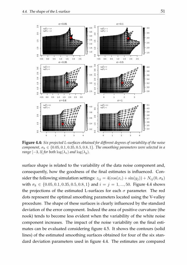
4.4. The shape of the L-surface 51
−0.5 0.0 0.5 1.0 1.5 2.0 2.5
0.5
1.0
1.5
2.0
2.5
σ = 0.05
xlim
1.0
1.5
2.0
2.5
3.0
3.5
4.0
log(λ)x = −1.5
log(λ)y = −1.5
−0.5 0.0 0.5 1.0 1.5 2.0 2.5
0.5
1.0
1.5
2.0
2.5
σ = 0.1
xlim
ylim
1.5
2.0
2.5
3.0
3.5
4.0
log(λ)x = −1
log(λ)y = −1
−0.5 0.0 0.5 1.0 1.5 2.0 2.5 3.0
0.5
1.0
1.5
2.0
2.5
3.0
σ = 0.35
xlim
2.5
3.0
3.5
4.0
log(λ)x = 0
log(λ)y = 0
0 1 2 30.
51.
01.
52.
02.
53.
03.
5
σ = 0.5
xlim
ylim
2.8
3.0
3.2
3.4
3.6
3.8
4.0
log(λ)x = 0
log(λ)y = 0
0 1 2 3 4
0.5
1.5
2.5
3.5
σ = 0.8
3.2
3.4
3.6
3.8
4.0
log(λ)x = 0.5
log(λ)y = 1
0 1 2 3 4
0.5
1.5
2.5
3.5
σ = 1
ylim
3.4
3.5
3.6
3.7
3.8
3.9
4.0
4.1
log(λ)x = 0.5
log(λ)y = 1
Figure 4.4: Six projected L-surfaces obtained for different degrees of variability of the noisecomponent, σk ∈ 0.05, 0.1, 0.35, 0.5, 0.8, 1. The smoothing parameters were selected in arange [−3, 3] for both log(λx) and log(λy).
surface shape is related to the variability of the data noise component and,consequently, how the goodness of the final estimates is influenced. Con-sider the following simulation settings: zij = 4(cos(xi) + sin(yj)) +Nij(0, σk)
with σk ∈ 0.05, 0.1, 0.35, 0.5, 0.8, 1 and i = j = 1, ..., 50. Figure 4.4 showsthe projections of the estimated L-surfaces for each σ parameter. The reddots represent the optimal smoothing parameters located using the V-valleyprocedure. The shape of these surfaces is clearly influenced by the standarddeviation of the error component. Indeed the area of positive curvature (thenook) tends to become less evident when the variability of the white noisecomponent increases. The impact of the noise variability on the final esti-mates can be evaluated considering figure 4.5. It shows the contours (solidlines) of the estimated smoothing surfaces obtained for four of the six stan-dard deviation parameters used in figure 4.4. The estimates are compared

52 Chapter 4. The L-surface for non-isotropic optimal smoothing
with the raw data (background of each plot). It appears that, even if theassociated L-surfaces are different, the smoothing surfaces efficiently catchthe data behavior. In order to better evaluate the impact of the variabilityof the noise component on the goodness of the final estimates we can use abigger simulation and evaluate the distributions of the (log) standardized de-viations of the estimated surfaces from the simulated data trend. Figure 4.6shows these distributions obtained for a grid of 10000 noisy points per eachσ parameter mentioned above. The mean deviations in figure 4.6 are all closeto zero but the variability of the distributions seems to increase together withthe variability of the noise component.
In analogy with the L-curve method, its multidimensional analogous,is robust to data with correlated noise (an example has been shown in fig-ure 4.1). In order to evaluate this feature we can consider a simulatedexperiment: generate 2500 observations according to zij = 4 cos(xi) +
4 sin(yj) + Eij(ρk) where x = y = −3, ..., 3 and Eij(ρ) represents the noiseterm. This noise component has been simulated in such a way to showserial correlation (in analogy with what we did for the example of fig-ure 4.1). The correlation structure has been induced considering smoothsurface obtained using a isotropic tensor product P-spline smoother. Hereρk = 0, 0.1, 0.3, 0.5, 0.75, 0.9 indicates the strength of the penalty imposedin the smoothing procedure used to obtain the noise component. The pro-jections of the L-surfaces resulting from these simulations are depicted infigure 4.7. All the surfaces of figure 4.7 show an area characterized by a clearnook where the optimal smoothing parameters have been located by a V-valley procedure (red dots). In addition, the smoothing surfaces in figure 4.8show how the estimated smoothers reproduce the underlying behavior forfour of the simulated data clouds. In order to evaluate how the goodnessof the final estimates is influenced by the degree of serial correlation in thenoise component, in analogy with what we did before, we can consider alarger simulation procedure. Figure 4.9 shows the distributions of the stan-dardized deviations of the final estimates from the underlying data trend fordifferent degree of serial correlation of the noise component. These boxplotshave been obtained considering a grid of 10000 observations. The standard-ized mean deviations are all close to zero and the shape of the distributionsis almost equal for each ρ parameter.
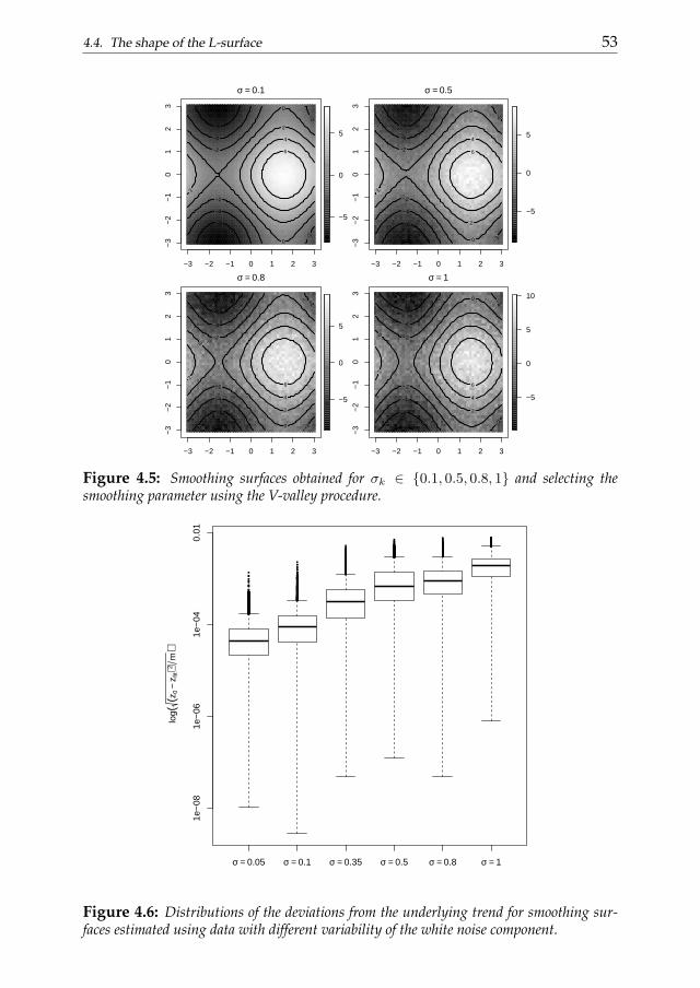
4.4. The shape of the L-surface 53
−3 −2 −1 0 1 2 3
−3
−2
−1
01
23
σ = 0.1
−5
0
5 −6
−6
−4
−4
−2
−2
−2
−2
0
0
2
2
4
6
−3 −2 −1 0 1 2 3
−3
−2
−1
01
23
σ = 0.5
−5
0
5
−6
−6
−4
−4
−2
−2
−2
−2 0
0
2
2
4
6
−3 −2 −1 0 1 2 3
−3
−2
−1
01
23
σ = 0.8
−5
0
5
−6
−6
−4
−4
−2
−2
−2
−2
0
0
2
2
4
6
−3 −2 −1 0 1 2 3
−3
−2
−1
01
23
σ = 1
−5
0
5
10
−8
−8
−6
−6
−4
−4
−2
−2
−2
−2
0
0
2
2
4
6
Figure 4.5: Smoothing surfaces obtained for σk ∈ 0.1, 0.5, 0.8, 1 and selecting thesmoothing parameter using the V-valley procedure.
log(
(z0
−z f
it)2m
)
σ = 0.05 σ = 0.1 σ = 0.35 σ = 0.5 σ = 0.8 σ = 1
1e−
081e
−06
1e−
040.
01
Figure 4.6: Distributions of the deviations from the underlying trend for smoothing sur-faces estimated using data with different variability of the white noise component.
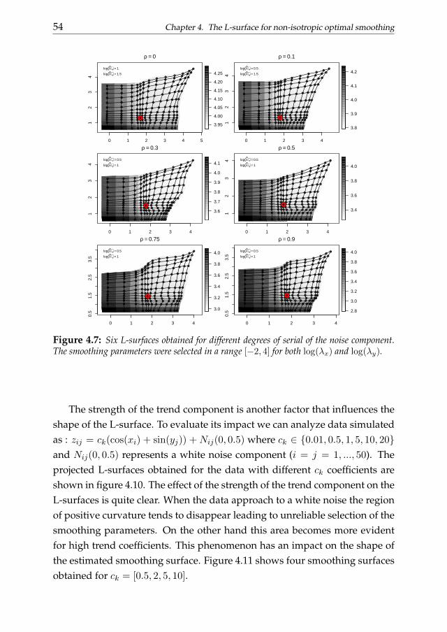
54 Chapter 4. The L-surface for non-isotropic optimal smoothing
0 1 2 3 4 5
12
34
ρ = 0
xlim
3.95
4.00
4.05
4.10
4.15
4.20
4.25
log(λ)x = 1
log(λ)y = 1.5
0 1 2 3 4
12
34
ρ = 0.1
xlim
ylim
3.8
3.9
4.0
4.1
4.2
log(λ)x = 0.5
log(λ)y = 1.5
0 1 2 3 4
12
34
ρ = 0.3
xlim
3.6
3.7
3.8
3.9
4.0
4.1
log(λ)x = 0.5
log(λ)y = 1
0 1 2 3 41
23
4
ρ = 0.5
xlim
ylim
3.4
3.6
3.8
4.0
log(λ)x = 0.5
log(λ)y = 1
0 1 2 3 4
0.5
1.5
2.5
3.5
ρ = 0.75
3.0
3.2
3.4
3.6
3.8
4.0
log(λ)x = 0.5
log(λ)y = 1
0 1 2 3 4
0.5
1.5
2.5
3.5
ρ = 0.9
ylim
2.8
3.0
3.2
3.4
3.6
3.8
4.0
log(λ)x = 0.5
log(λ)y = 1
Figure 4.7: Six L-surfaces obtained for different degrees of serial of the noise component.The smoothing parameters were selected in a range [−2, 4] for both log(λx) and log(λy).
The strength of the trend component is another factor that influences theshape of the L-surface. To evaluate its impact we can analyze data simulatedas : zij = ck(cos(xi) + sin(yj)) + Nij(0, 0.5) where ck ∈ 0.01, 0.5, 1, 5, 10, 20and Nij(0, 0.5) represents a white noise component (i = j = 1, ..., 50). Theprojected L-surfaces obtained for the data with different ck coefficients areshown in figure 4.10. The effect of the strength of the trend component on theL-surfaces is quite clear. When the data approach to a white noise the regionof positive curvature tends to disappear leading to unreliable selection of thesmoothing parameters. On the other hand this area becomes more evidentfor high trend coefficients. This phenomenon has an impact on the shape ofthe estimated smoothing surface. Figure 4.11 shows four smoothing surfacesobtained for ck = [0.5, 2, 5, 10].

4.4. The shape of the L-surface 55
−3 −2 −1 0 1 2 3
−3
−2
−1
01
23
ρ = 0
−10
−5
0
5
10
−8
−6
−6
−4
−4
−2
−2
−2
0
0
2
4
6
−3 −2 −1 0 1 2 3
−3
−2
−1
01
23
ρ = 0.3
−10
−5
0
5
10
−8
−8
−6
−6
−4
−4
−2
−2
−2
0
0
2
4
6
−3 −2 −1 0 1 2 3
−3
−2
−1
01
23
ρ = 0.75
−5
0
5
−6
−6
−4
−4
−2
−2
−2
−2
0
0
2
2
4
6
−3 −2 −1 0 1 2 3
−3
−2
−1
01
23
ρ = 0.9
−5
0
5
−8
−6
−6
−4
−4
−2
−2
−2
−2
0
0
2
2
4
6
8
Figure 4.8: Contours of the smoothing surfaces obtained for ρk ∈ 0, 0.3, 0.75, 0.9. Thebackground of each plot represents the raw data.
log(
(z0
−z f
it)2m
)
ρ = 0 ρ = 0.1 ρ = 0.3 ρ = 0.5 ρ = 0.75 ρ = 0.9
1e−
061e
−05
1e−
040.
001
0.01
Figure 4.9: Distributions of the deviations from the underlying trend for smoothing sur-faces estimated using data with different serial correlation of the noise component.
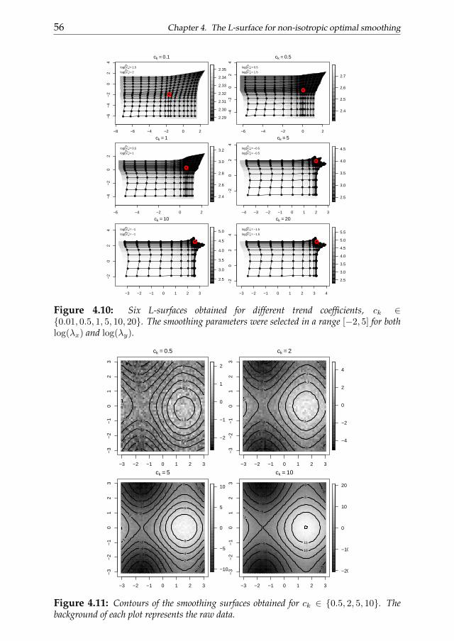
56 Chapter 4. The L-surface for non-isotropic optimal smoothing
−8 −6 −4 −2 0 2
−6
−4
−2
02
4
ck = 0.1
xlim
2.29
2.30
2.31
2.32
2.33
2.34
2.35
log(λ)x = 1.5
log(λ)y = 2
−6 −4 −2 0 2
−4
−2
02
4
ck = 0.5
xlim
ylim
2.4
2.5
2.6
2.7
log(λ)x = 0.5
log(λ)y = 1.5
−6 −4 −2 0 2
−4
−2
02
ck = 1
xlim
2.4
2.6
2.8
3.0
3.2
log(λ)x = 0.5
log(λ)y = 1
−4 −3 −2 −1 0 1 2 3
−2
02
4
ck = 5
xlimyl
im
2.5
3.0
3.5
4.0
4.5
log(λ)x = −0.5
log(λ)y = −0.5
−3 −2 −1 0 1 2 3
−2
02
4
ck = 10
2.5
3.0
3.5
4.0
4.5
5.0
log(λ)x = −1
log(λ)y = −1
−3 −2 −1 0 1 2 3 4
−2
02
4
ck = 20yl
im
2.5
3.0
3.5
4.0
4.5
5.0
5.5
log(λ)x = −1.5
log(λ)y = −1.5
Figure 4.10: Six L-surfaces obtained for different trend coefficients, ck ∈0.01, 0.5, 1, 5, 10, 20. The smoothing parameters were selected in a range [−2, 5] for bothlog(λx) and log(λy).
−3 −2 −1 0 1 2 3
−3
−2
−1
01
23
ck = 0.5
−2
−1
0
1
2
−1
−0.8
−0.8
−0.6
−0.6
−0.4
−0.4
−0.2
−0.2
0
0
0.2
0.2
0.4
0.6
0.8
−3 −2 −1 0 1 2 3
−3
−2
−1
01
23
ck = 2
−4
−2
0
2
4
−4
−4
−3
−3
−2
−2
−1
−1
−1
−1
0
0
1
1
2
3
−3 −2 −1 0 1 2 3
−3
−2
−1
01
23
ck = 5
−10
−5
0
5
10
−8
−8
−6
−6
−4
−4
−2
−2
−2
−2
0
0
2
2
4
6
8
−3 −2 −1 0 1 2 3
−3
−2
−1
01
23
ck = 10
−20
−10
0
10
20
−15
−15
−10
−10
−5
−5
−5
−5
0
0
5
5
10
15
Figure 4.11: Contours of the smoothing surfaces obtained for ck ∈ 0.5, 2, 5, 10. Thebackground of each plot represents the raw data.

4.5. Some examples 57
4.5 Some examples
In this section some application of the L-surface selection procedure areshown. We consider both simulated and real data examples. As first appli-cation we consider the de-noise of a simulated image. The left upper panelof figure 4.12 depicts a a grid of 90 × 90 pixels describing a quarter of circleto whom a random noise have been added. This example is analogous to theexperiment proposed by Eilers et al. (2006). The height of the simulated sur-face is indicated by the intensity of the image with a light color indicating agreater height. The right upper panel of the same figure shows the enhancedimage obtained using a P-spline smoother built on a grid of 22 × 22 tensorproduct B-splines and applying third order penalty matrices to both direc-tions. The optimal smoothing parameters have been selected using the L-surface criterion: log(λx) = 1.5 and log(λy) = 1.5 (see right panel of the lowerpart of the figure obtained considering a log(λx) = log(λy) ∈ −1, 3 grid ofpossible smoothing parameter). The left lower panel shows the residuals be-tween the original and the smoothed image. The results obtained selectingthe smoothing parameter by cross validation on the same grid of candidateλs are shown in figure 4.13. The two selection procedures give comparableresults given that the cross validation suggests log(λx) = log(λy) = 1.
As second example we analyze the monthly total precipitation (mm) forApril 1948 in the contiguous United States described in a dataset discussedin Johns et al. (2003). The data and the smoothed precipitation over theUS are showed in figure 4.14. The upper panels of this figure show theraw data (left panel) and the smoothed data obtained without consideringthe boundaries. In the lower panels the smoothed data and the projectedL-surface associated are shown. The smoothed image have been obtainedconsidering 10 cubic bases on the x and y directions and the penalties werebuilt using 3th order difference matrices. The optimal smoothing parame-ter on the L-surface has been selected using the V-valley criterion describedabove computed over a grid of candidate parameters defined in the inter-val log(λx) = log(λy) ∈ −1, 4. The selected smoothing parameters wereλx = 0.5 and λy = −0.5. Figure 4.15 shows the results obtained for thesame data smoothing the raw observations using the λ parameters selectedby cross validation. As we can see the cross validation surface appears flat
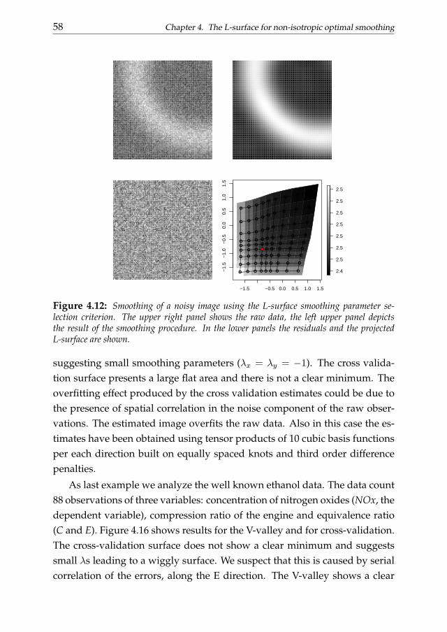
58 Chapter 4. The L-surface for non-isotropic optimal smoothing
−1.5 −0.5 0.0 0.5 1.0 1.5
−1.
5−
1.0
−0.
50.
00.
51.
01.
5
ylim
2.49
2.50
2.51
2.52
2.53
2.54
2.55
2.56
Figure 4.12: Smoothing of a noisy image using the L-surface smoothing parameter se-lection criterion. The upper right panel shows the raw data, the left upper panel depictsthe result of the smoothing procedure. In the lower panels the residuals and the projectedL-surface are shown.
suggesting small smoothing parameters (λx = λy = −1). The cross valida-tion surface presents a large flat area and there is not a clear minimum. Theoverfitting effect produced by the cross validation estimates could be due tothe presence of spatial correlation in the noise component of the raw obser-vations. The estimated image overfits the raw data. Also in this case the es-timates have been obtained using tensor products of 10 cubic basis functionsper each direction built on equally spaced knots and third order differencepenalties.
As last example we analyze the well known ethanol data. The data count88 observations of three variables: concentration of nitrogen oxides (NOx, thedependent variable), compression ratio of the engine and equivalence ratio(C and E). Figure 4.16 shows results for the V-valley and for cross-validation.The cross-validation surface does not show a clear minimum and suggestssmall λs leading to a wiggly surface. We suspect that this is caused by serialcorrelation of the errors, along the E direction. The V-valley shows a clear

4.6. Conclusions 59
325
330
335
340
345
350
−1 0 1 2 3
−1
01
23
Figure 4.13: Smoothing of a noisy image using the cross validation smoothing parameterselection criterion. The upper right panel shows the raw data, the left upper panel depicts theresult of the smoothing procedure. In the lower panels the residuals and the cross validationsurface are shown.
minimum and leads to a smooth surface with intuitive appeal.
4.6 Conclusions
We have shown how the concept of the L-curve can be extended to two-dimensional smoothing with tensor product P-splines. A natural two dimen-sional generalization of the L-curve is represented by the L-surface. The L-surface is defined by a set of 1D L-curve computed in the x and y directions.Each L-curve has a convex area and the points defining them become closerand in the proximity of the corner. The Euclidean distance between adjacentpoints on a single L-curve is described by a V-shaped curve and the singledimensional optimal smoothing parameter is located at the minimum of theV-curve.
This combination of L-curves generates the characteristic shape of the L-surface. The L-surface has a nook in which the right balance between theresidual sum of squares and two penalties is found. This nook corresponds
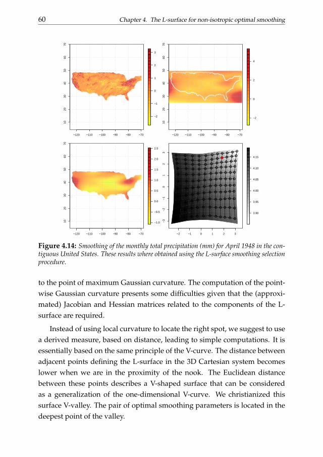
60 Chapter 4. The L-surface for non-isotropic optimal smoothing
−120 −110 −100 −90 −80 −70
1020
3040
5060
70
Longitude
−2
−1
0
1
2
3
−120 −110 −100 −90 −80 −70
1020
3040
5060
70
Longitude
Latit
ude
−2
0
2
4
−120 −110 −100 −90 −80 −70
1020
3040
5060
70
−1.0
−0.5
0.0
0.5
1.0
1.5
2.0
2.5
−2 −1 0 1 2 3
−3
−2
−1
01
23
Ψ2
3.90
3.95
4.00
4.05
4.10
4.15
Figure 4.14: Smoothing of the monthly total precipitation (mm) for April 1948 in the con-tiguous United States. These results where obtained using the L-surface smoothing selectionprocedure.
to the point of maximum Gaussian curvature. The computation of the point-wise Gaussian curvature presents some difficulties given that the (approxi-mated) Jacobian and Hessian matrices related to the components of the L-surface are required.
Instead of using local curvature to locate the right spot, we suggest to usea derived measure, based on distance, leading to simple computations. It isessentially based on the same principle of the V-curve. The distance betweenadjacent points defining the L-surface in the 3D Cartesian system becomeslower when we are in the proximity of the nook. The Euclidean distancebetween these points describes a V-shaped surface that can be consideredas a generalization of the one-dimensional V-curve. We christianized thissurface V-valley. The pair of optimal smoothing parameters is located in thedeepest point of the valley.
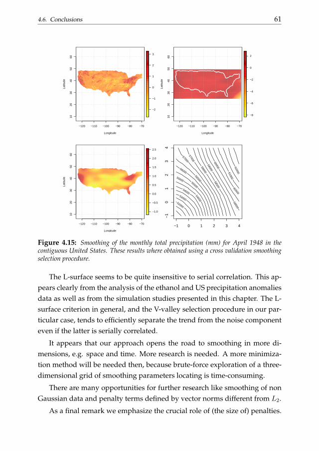
4.6. Conclusions 61
−120 −110 −100 −90 −80 −70
1020
3040
5060
Longitude
Latit
ude
−2
−1
0
1
2
3
−120 −110 −100 −90 −80 −70
1020
3040
5060
Longitude
Latit
ude
−8
−6
−4
−2
0
2
−120 −110 −100 −90 −80 −70
1020
3040
5060
Longitude
Latit
ude
−1.0
−0.5
0.0
0.5
1.0
1.5
2.0
2.5
52000
53000
54000 54500
55000 55500
56000
56500
57000 57500
58000
58500
59000
59500
60000
60500
61000 62000
−1 0 1 2 3 4
−1
01
23
4
Figure 4.15: Smoothing of the monthly total precipitation (mm) for April 1948 in thecontiguous United States. These results where obtained using a cross validation smoothingselection procedure.
The L-surface seems to be quite insensitive to serial correlation. This ap-pears clearly from the analysis of the ethanol and US precipitation anomaliesdata as well as from the simulation studies presented in this chapter. The L-surface criterion in general, and the V-valley selection procedure in our par-ticular case, tends to efficiently separate the trend from the noise componenteven if the latter is serially correlated.
It appears that our approach opens the road to smoothing in more di-mensions, e.g. space and time. More research is needed. A more minimiza-tion method will be needed then, because brute-force exploration of a three-dimensional grid of smoothing parameters locating is time-consuming.
There are many opportunities for further research like smoothing of nonGaussian data and penalty terms defined by vector norms different from L2.
As a final remark we emphasize the crucial role of (the size of) penalties.
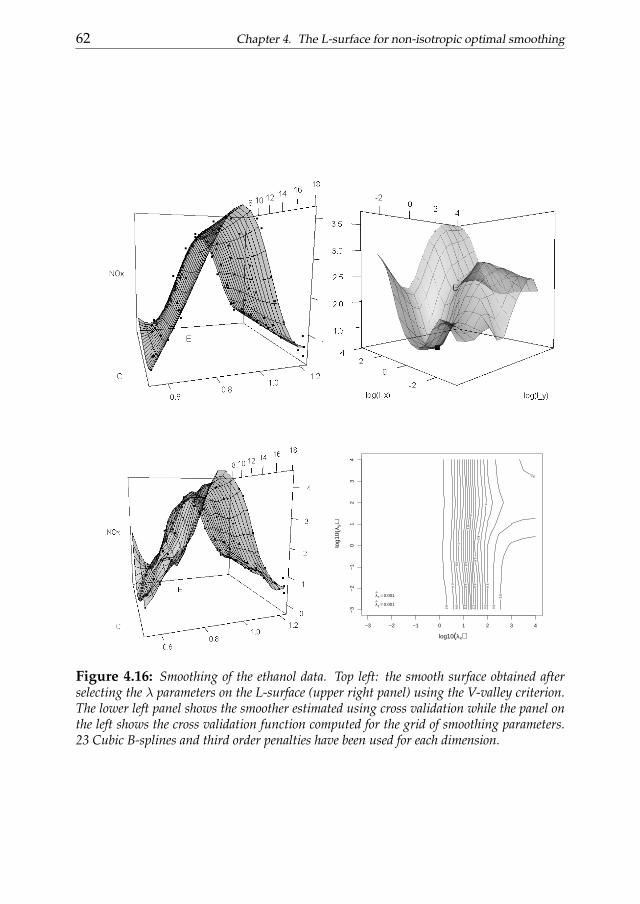
62 Chapter 4. The L-surface for non-isotropic optimal smoothing
log10(λx)
log1
0(λ y
)
0.2
0.4 0.6
0.8
1
1.2 1.4
1.6
1.8
2
2.2 2.4
2.6
2.8
3
3.2
3.4
3.6
3.6
3.8
−3 −2 −1 0 1 2 3 4
−3
−2
−1
01
23
4
λx = 0.001
λy = 0.001
Figure 4.16: Smoothing of the ethanol data. Top left: the smooth surface obtained afterselecting the λ parameters on the L-surface (upper right panel) using the V-valley criterion.The lower left panel shows the smoother estimated using cross validation while the panel onthe left shows the cross validation function computed for the grid of smoothing parameters.23 Cubic B-splines and third order penalties have been used for each dimension.

4.6. Conclusions 63
Smoothing methods like kernels and local likelihood do not have an equiva-lent and so they cannot profit from the L-curve and its extensions.

THE B SPLINE COLLOCATION PROCEDURE 5In this chapter we introduce the B-spline collocation procedure. We
treat both ordinary and partial differential problems with initial andboundary conditions. The collocation scheme is applied to the Black andScholes equation for the pricing of European option contracts. The ap-proximated prices are compared with the analytic solution of the cited dif-ferential problem to evaluate the performance of the proposed numericalscheme.Keywords: Ordinary/partial differential equations, collocation, B-splines, European option pricing.
5.1 Introduction
Differential equations are powerful tools for describing system’s dynamics.In many circumstances it is advantageous to have at our disposal a proce-dure to numerically approximate the solution. This is the case when dealingwith problems that cannot be solved analytically or if we are interested ininferring the characteristics of a phenomenon which’ dynamics is describedby observed data, as introduced in chapter 1.
Several numerical procedures have been proposed in the literature tosolve ordinary and partial differential problems. The main idea of a nu-merical method is to replace the DE, formulated for one unknown real val-ued function, by a discrete equation in finitely many unknowns. The dis-crete problem defines the so called ”numerical scheme”. For a completeoverview about the different numerical methods proposed in the literaturea well known reference is Ascher and Petzold (1998).
Here we introduce the collocation method and discuss it in the case of lin-ear differential problems. The collocation method belongs to the more gen-
65
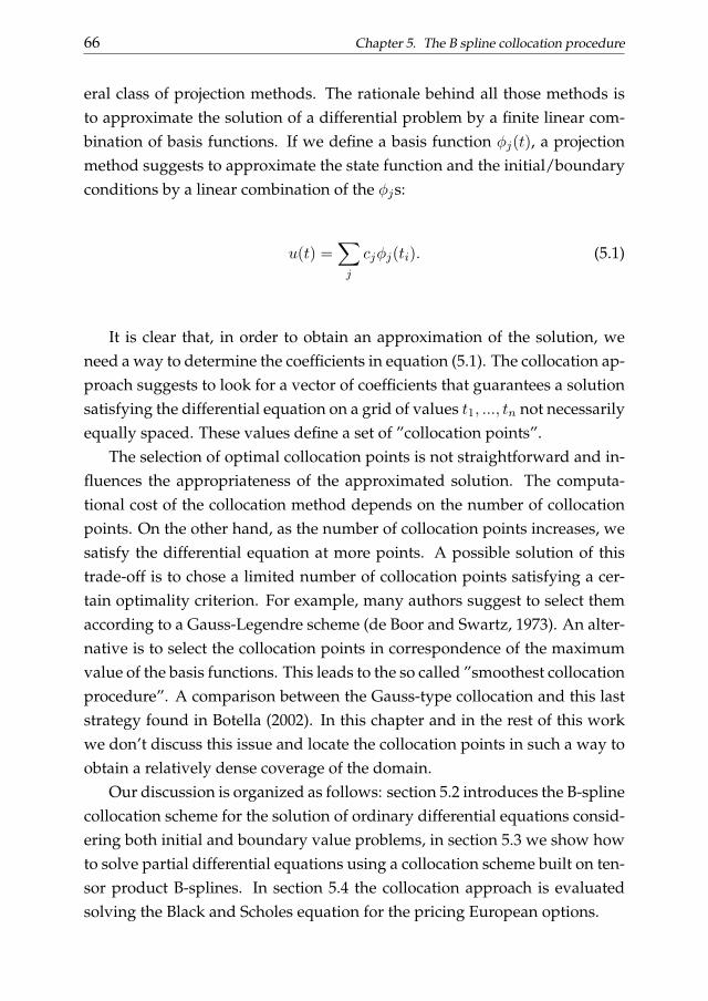
66 Chapter 5. The B spline collocation procedure
eral class of projection methods. The rationale behind all those methods isto approximate the solution of a differential problem by a finite linear com-bination of basis functions. If we define a basis function φj(t), a projectionmethod suggests to approximate the state function and the initial/boundaryconditions by a linear combination of the φjs:
u(t) =∑j
cjφj(ti). (5.1)
It is clear that, in order to obtain an approximation of the solution, weneed a way to determine the coefficients in equation (5.1). The collocation ap-proach suggests to look for a vector of coefficients that guarantees a solutionsatisfying the differential equation on a grid of values t1, ..., tn not necessarilyequally spaced. These values define a set of ”collocation points”.
The selection of optimal collocation points is not straightforward and in-fluences the appropriateness of the approximated solution. The computa-tional cost of the collocation method depends on the number of collocationpoints. On the other hand, as the number of collocation points increases, wesatisfy the differential equation at more points. A possible solution of thistrade-off is to chose a limited number of collocation points satisfying a cer-tain optimality criterion. For example, many authors suggest to select themaccording to a Gauss-Legendre scheme (de Boor and Swartz, 1973). An alter-native is to select the collocation points in correspondence of the maximumvalue of the basis functions. This leads to the so called ”smoothest collocationprocedure”. A comparison between the Gauss-type collocation and this laststrategy found in Botella (2002). In this chapter and in the rest of this workwe don’t discuss this issue and locate the collocation points in such a way toobtain a relatively dense coverage of the domain.
Our discussion is organized as follows: section 5.2 introduces the B-splinecollocation scheme for the solution of ordinary differential equations consid-ering both initial and boundary value problems, in section 5.3 we show howto solve partial differential equations using a collocation scheme built on ten-sor product B-splines. In section 5.4 the collocation approach is evaluatedsolving the Black and Scholes equation for the pricing European options.
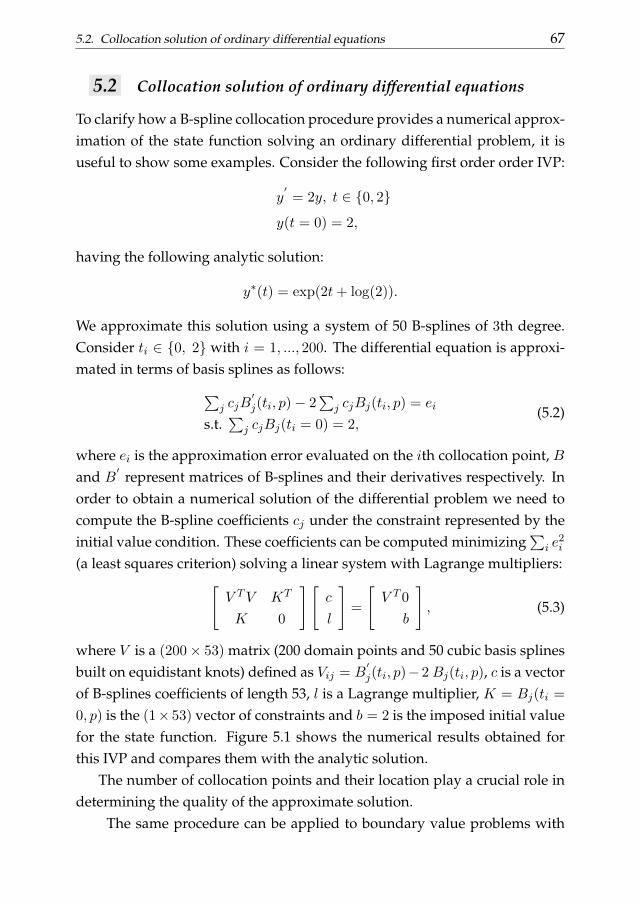
5.2. Collocation solution of ordinary differential equations 67
5.2 Collocation solution of ordinary differential equations
To clarify how a B-spline collocation procedure provides a numerical approx-imation of the state function solving an ordinary differential problem, it isuseful to show some examples. Consider the following first order order IVP:
y′
= 2y, t ∈ 0, 2
y(t = 0) = 2,
having the following analytic solution:
y∗(t) = exp(2t+ log(2)).
We approximate this solution using a system of 50 B-splines of 3th degree.Consider ti ∈ 0, 2 with i = 1, ..., 200. The differential equation is approxi-mated in terms of basis splines as follows:∑
j cjB′j(ti, p)− 2
∑j cjBj(ti, p) = ei
s.t.∑
j cjBj(ti = 0) = 2,(5.2)
where ei is the approximation error evaluated on the ith collocation point, Band B
′represent matrices of B-splines and their derivatives respectively. In
order to obtain a numerical solution of the differential problem we need tocompute the B-spline coefficients cj under the constraint represented by theinitial value condition. These coefficients can be computed minimizing
∑i e
2i
(a least squares criterion) solving a linear system with Lagrange multipliers:[V TV KT
K 0
][c
l
]=
[V T 0
b
], (5.3)
where V is a (200× 53) matrix (200 domain points and 50 cubic basis splinesbuilt on equidistant knots) defined as Vij = B
′j(ti, p)−2 Bj(ti, p), c is a vector
of B-splines coefficients of length 53, l is a Lagrange multiplier, K = Bj(ti =
0, p) is the (1× 53) vector of constraints and b = 2 is the imposed initial valuefor the state function. Figure 5.1 shows the numerical results obtained forthis IVP and compares them with the analytic solution.
The number of collocation points and their location play a crucial role indetermining the quality of the approximate solution.
The same procedure can be applied to boundary value problems with
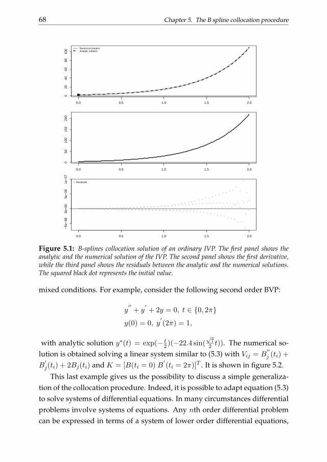
68 Chapter 5. The B spline collocation procedure
0.0 0.5 1.0 1.5 2.0
020
4060
8010
0 Numerical solutionAnalytic solution
0.0 0.5 1.0 1.5 2.0
050
100
150
200
0.0 0.5 1.0 1.5 2.0
−5e
−08
0e+
005e
−08
1e−
07
Residuals
Figure 5.1: B-splines collocation solution of an ordinary IVP. The first panel shows theanalytic and the numerical solution of the IVP. The second panel shows the first derivative,while the third panel shows the residuals between the analytic and the numerical solutions.The squared black dot represents the initial value.
mixed conditions. For example, consider the following second order BVP:
y′′
+ y′+ 2y = 0, t ∈ 0, 2π
y(0) = 0, y′(2π) = 1,
with analytic solution y∗(t) = exp(− t2)(−22.4 sin(
√7
2 t)). The numerical so-lution is obtained solving a linear system similar to (5.3) with Vij = B
′′j (ti) +
B′j(ti) + 2Bj(ti) and K = [B(ti = 0) B
′(ti = 2π)]T . It is shown in figure 5.2.
This last example gives us the possibility to discuss a simple generaliza-tion of the collocation procedure. Indeed, it is possible to adapt equation (5.3)to solve systems of differential equations. In many circumstances differentialproblems involve systems of equations. Any nth order differential problemcan be expressed in terms of a system of lower order differential equations,
5.2. Collocation solution of ordinary differential equations 69
0 1 2 3 4 5 6
−10
−5
0
Numerical solutionAnalytic solution
0 1 2 3 4 5 6
−30
−10
010
0 1 2 3 4 5 6
−10
010
2030
0 1 2 3 4 5 6
0e+
001e
−03 Residuals
Figure 5.2: B-splines collocation solution of an ordinary second order BVP. The first panelshows the analytic and the numerical solution of the differential problem. The second andthird panels show the first and second derivatives respectively, while the fourth panel showsthe residuals between the analytic and the numerical solutions. The squared blacks dot in-dicate the boundary values. The approximate solution has been obtained using 50 equallyspaced cubic B-splines.
and in many cases it is convenient to deal with lower order derivatives. TheBVP above can be translated in the following system:
x′1 = x2
x′2 = −2x1 − x2
x1(0) = 0, x2(2π) = 1,
(5.4)
where the change of variables y = x1, y′
= x2 has been applied.In this case the least squares system in (5.3) can be generalized. Each of
the two top equations in (5.4) leads to residuals as in (5.2) that have to beminimized through leasr squares. One way to compute the optimal splinecoefficients is to define the linear system in terms of Kronecker products. In
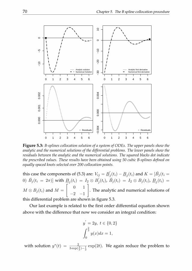
70 Chapter 5. The B spline collocation procedure
0 1 2 3 4 5 6
−10
−5
0
x
Analytic solutionNumerical Solution
0 1 2 3 4 5 6
−30
−20
−10
010
x
y1
Analytic first derivativeNumerical first derivative
0 1 2 3 4 5 6
0.00
00.
001
0.00
2
Residuals
0 1 2 3 4 5 6
−0.
004
0.00
00.
004
fit[,
2] −
y1
Residuals
Figure 5.3: B-splines collocation solution of a system of ODEs. The upper panels show theanalytic and the numerical solutions of the differential problems. The lower panels show theresiduals between the analytic and the numerical solutions. The squared blacks dot indicatethe prescribed values. These results have been obtained using 50 cubic B-splines defined onequally spaced knots selected over 200 collocation points.
this case the components of (5.3) are: Vij = B′j(ti)−Bj(ti) and K = [Bj(ti =
0) Bj(ti = 2π)] with Bj(ti) = I2 ⊗ B′j(ti), Bj(ti) = I2 ⊗ Bj(ti), Bj(ti) =
M ⊗ Bj(ti) and M =
[0 1
−2 −1
]. The analytic and numerical solutions of
this differential problem are shown in figure 5.3.Our last example is related to the first order differential equation shown
above with the difference that now we consider an integral condition:
y′
= 2y, t ∈ 0, 2∫ 23
0y(x)dx = 1,
with solution y∗(t) = 23 exp( 2
3)− 1
2
exp(2t). We again reduce the problem to
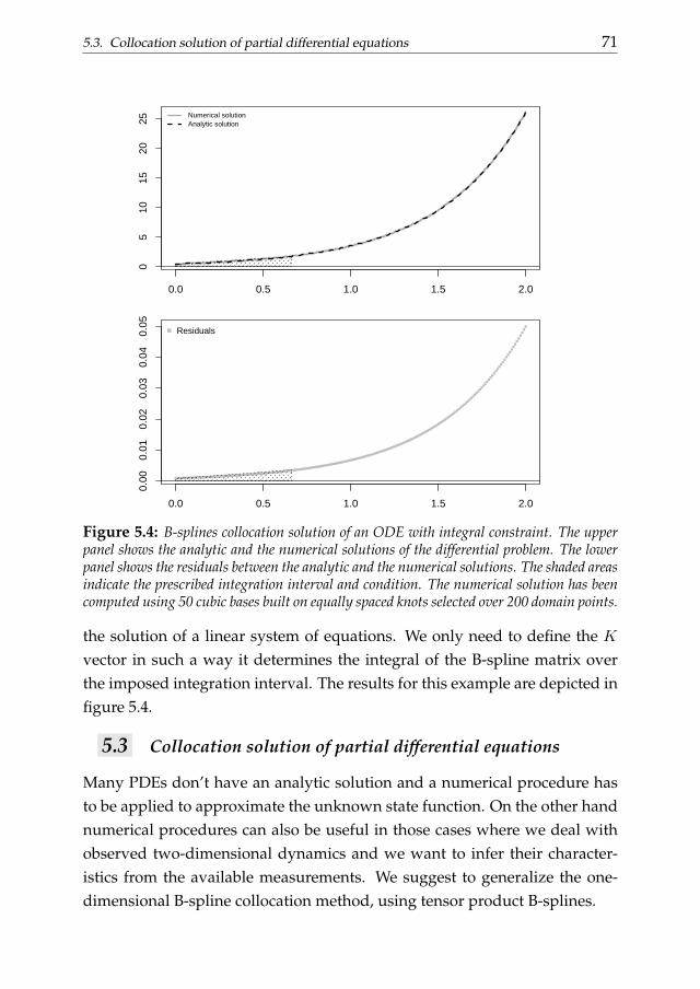
5.3. Collocation solution of partial differential equations 71
0.0 0.5 1.0 1.5 2.0
05
1015
2025
Numerical solutionAnalytic solution
0.0 0.5 1.0 1.5 2.0
0.00
0.01
0.02
0.03
0.04
0.05
Residuals
Figure 5.4: B-splines collocation solution of an ODE with integral constraint. The upperpanel shows the analytic and the numerical solutions of the differential problem. The lowerpanel shows the residuals between the analytic and the numerical solutions. The shaded areasindicate the prescribed integration interval and condition. The numerical solution has beencomputed using 50 cubic bases built on equally spaced knots selected over 200 domain points.
the solution of a linear system of equations. We only need to define the Kvector in such a way it determines the integral of the B-spline matrix overthe imposed integration interval. The results for this example are depicted infigure 5.4.
5.3 Collocation solution of partial differential equations
Many PDEs don’t have an analytic solution and a numerical procedure hasto be applied to approximate the unknown state function. On the other handnumerical procedures can also be useful in those cases where we deal withobserved two-dimensional dynamics and we want to infer their character-istics from the available measurements. We suggest to generalize the one-dimensional B-spline collocation method, using tensor product B-splines.
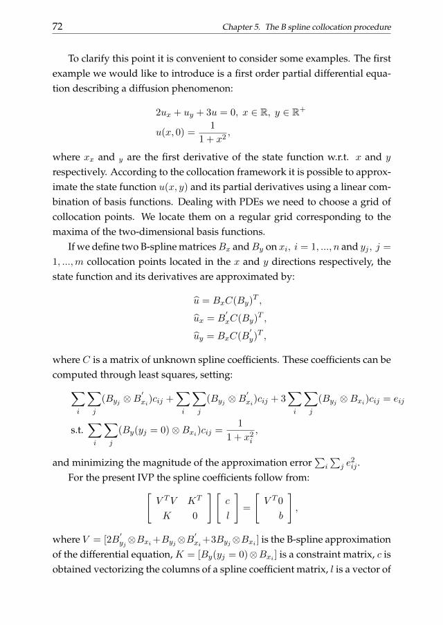
72 Chapter 5. The B spline collocation procedure
To clarify this point it is convenient to consider some examples. The firstexample we would like to introduce is a first order partial differential equa-tion describing a diffusion phenomenon:
2ux + uy + 3u = 0, x ∈ R, y ∈ R+
u(x, 0) =1
1 + x2,
where xx and y are the first derivative of the state function w.r.t. x and y
respectively. According to the collocation framework it is possible to approx-imate the state function u(x, y) and its partial derivatives using a linear com-bination of basis functions. Dealing with PDEs we need to choose a grid ofcollocation points. We locate them on a regular grid corresponding to themaxima of the two-dimensional basis functions.
If we define two B-spline matricesBx andBy on xi, i = 1, ..., n and yj , j =
1, ...,m collocation points located in the x and y directions respectively, thestate function and its derivatives are approximated by:
u = BxC(By)T ,
ux = B′xC(By)
T ,
uy = BxC(B′y)T ,
where C is a matrix of unknown spline coefficients. These coefficients can becomputed through least squares, setting:∑
i
∑j
(Byj ⊗B′xi)cij +
∑i
∑j
(Byj ⊗B′xi)cij + 3
∑i
∑j
(Byj ⊗Bxi)cij = eij
s.t.∑i
∑j
(By(yj = 0)⊗Bxi)cij =1
1 + x2i
,
and minimizing the magnitude of the approximation error∑
i
∑j e
2ij .
For the present IVP the spline coefficients follow from:[V TV KT
K 0
][c
l
]=
[V T 0
b
],
where V = [2B′yj⊗Bxi+Byj⊗B
′xi+3Byj⊗Bxi ] is the B-spline approximation
of the differential equation, K = [By(yj = 0)⊗Bxi ] is a constraint matrix, c isobtained vectorizing the columns of a spline coefficient matrix, l is a vector of
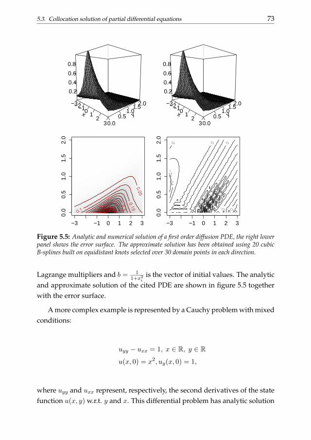
5.3. Collocation solution of partial differential equations 73
x
−3−2−101
23
y
0.00.5
1.01.5
2.0
0.2
0.4
0.6
0.8
x
−3−2−101
23
y
0.00.5
1.01.5
2.0
0.2
0.4
0.6
0.8
−3 −1 0 1 2 3
0.0
0.5
1.0
1.5
2.0
−3 −1 0 1 2 3
0.0
0.5
1.0
1.5
2.0
Figure 5.5: Analytic and numerical solution of a first order diffusion PDE, the right lowerpanel shows the error surface. The approximate solution has been obtained using 20 cubicB-splines built on equidistant knots selected over 30 domain points in each direction.
Lagrange multipliers and b = 11+x2i
is the vector of initial values. The analyticand approximate solution of the cited PDE are shown in figure 5.5 togetherwith the error surface.
A more complex example is represented by a Cauchy problem with mixedconditions:
uyy − uxx = 1, x ∈ R, y ∈ R
u(x, 0) = x2, uy(x, 0) = 1,
where uyy and uxx represent, respectively, the second derivatives of the statefunction u(x, y) w.r.t. y and x. This differential problem has analytic solution

74 Chapter 5. The B spline collocation procedure
x
−20−10
010
20
y
05
1015
20
200
400
600
800
1000
x
−20−10
010
20
y
05
1015
20
200
400
600
800
1000
−20 −10 0 10 20
05
1015
20
−20 −10 0 10 20
05
1015
20
Figure 5.6: Analytic and numerical solution of a second order Cauchy PDE, the right lowerpanel shows the error surface. The state function has been approximated using fourth orderbasis splines defined on 15 equally spaced knots in each direction.
u∗(x, y) = x2 + y + 1.5y2. We now have:
u = BxC(By)T ,
uxx = B′′xC(By)
T ,
uyy = BxC(B′′y )T ,
uy = BxC(B′y)T .
The optimal spline coefficients c are computed solving a system of equationssimilar to (5.3), with Vij = [B
′′yj ⊗ Bxi − Byj ⊗ B
′′xi − 1], K = [By(yj = 0) ⊗
Bx B′y(yi = 0) ⊗ Bxi ]
T , b = [x2 1]T . Figure 5.6 compares the analytic andnumerical solutions.
5.4. Option pricing through B-spline collocation 75
5.4 Option pricing through B-spline collocation
To evaluate the performance of the B-spline collocation scheme introducedin the previous section we propose to solve the Black and Scholes equation(Black and Scholes, 1973) and compare the approximated and the exact solu-tions.
The B&S equation is the most famous mathematical pricing model forEuropean style financial options. Quoting Cox et al. (1979), an option is acontract that gives the right, but not the obligation, to buy or sell a risky assetat a predetermined fixed price within a specified period. This contract allowsto bet about the future evolution of the price of the underlying asset. Theunderlying can be a financial instrument (a stock for example), a financialindex and also a commodity. Options and other related contracts are oftendefined financial ”derivatives”. It is because their price is derived from themarket value of the underlying risky asset.
Two different kinds of option contracts are distinguished according to theright that they give to the holder. A ”call” is a contract that gives the rightto buy the underlying asset while a ”put” gives the right to sell it. Thesecharacteristics can be summarized in the payoffs function at expiration (ma-turity) time T associated to these two different contracts. If we indicate withC(S, T ) the payoff of a call at maturity and with P (S, T ) the payoff of a put,the definition above can be summarized as follows:
C(S, T ) =
0 if ST ≤ EST − E if ST > E,
P (S, T ) =
0 if ST ≥ EE − ST if ST < E,
where with E we indicate the strike price (the predetermined price of theunderlying at expiration time) and ST represents its market price at maturity.
The Black and Scholes model moves from the assumption that the dy-namics of the price of the underlying risky asset follows a geometric Brown-ian motion in the instantaneous time dt with mean µ and standard deviationσ√dt. Consider a option written on a share. If, in analogy with the previous
notation, we indicate with S the stock price this assumption implies that:
dS
S∼ φ
(µdt, σ2dt
), (5.5)
76 Chapter 5. The B spline collocation procedure
where dS is the stock price variation at instant dt and φ(·) indicates a Gaus-sian probability density function. If ST is the stock price at maturity time thisdynamics implies that:
ln(ST )− ln(S0) ∼ φ[(µ− σ2
2
)T, σ2T
],
(5.6)
ln(ST ) ∼ φ[ln(S0) +
(µ− σ2
2
)T, σ2T
].
This implies that ST follows a log-normal distribution such that E(ST ) =
S0 expµT and Var(ST ) = S20 exp2µT[expσ2T − 1]. The dynamic of S
under these assumptions are then described by:
dS = µSdt+ σSdz. (5.7)
Let V (S, t) be the value of the derivative contract. Following the defini-tion of an option contract its price depends on: the maturity date T (or betterof the time to maturity t− T ), the risk free interest rate r, the volatility of theunderlying asset σ, the strike price E and the spot price of the underlying S.Those variables are all included in the B&S model. Indeed, this model statesthat the mathematical law governing the value of the option can be writtenas the PDE:
∂V
∂t+ rS
∂V
∂S+
1
2σ2S2∂
2V
∂S2= rV. (5.8)
The solution depends on the boundary conditions that define the valueof the derivative contract for extreme values of S and t. The boundary condi-tions are defined to be consistent with the payoff functions. Consider a plainvanilla (which price does not depends on accessory rights) European call op-tion written on a stock that does not pay dividends. In this case the boundaryconditions for the differential problem (5.8) are:
C(0, t) = 0
C(S, t) = S − E exp−r(T − t) for large S
On the other hand the terminal condition, the boundary condition de-fined for t = T , can be written as:
C(S, T ) = max(S − E, 0) = (S − E)+
5.4. Option pricing through B-spline collocation 77
Analogous terminal and boundary conditions hold for a vanilla Europeanput option. Given those conditions the solution of (5.8), for a call and a putoption respectively is:
C(S, t) = S0Φ(d1)− E exp−rtΦ(d2)
(5.9)
P (S, t) = E exp−rtΦ(−d2)− S0Φ(−d1)
where Φ(·) indicates the standard normal cumulative distribution functionand:
d1 =ln(S0/E) + (rtσ2/2)T
σ√T
,
d2 = d1 − σ√T .
5.4.1 Pricing a plain vanilla European call option
An European vanilla call option is a contract giving to the owner the rightto buy a share of a specific common stock (whose price is S(t) at time t) ata fixed price E at a certain date T . In the previous introduction we havedefined the Black and Scholes equation for the value C(S, t) of an Europeancall option on an asset of value of value with a given volatility and interestrate. As we showed there exists a closed form solution of the B&S equationfor this kind of option contract. It gives us the possibility to test the qualityof the numerical solution achieved through the proposed B-spline collocationscheme.
As an example, we consider an European vanilla call option with exerciseprice E = 100, volatility σ2 = 0.32, risk free rate r = 0.1, and exercise time1 year. The change of variables U(x, τ) = 1
EV (E exp(Lx), k) with τ = T − t,x ∈ [−1, 1], k = 2τ/σ2 and L = −r(T−t) leads to the following reformulationof (5.8):
∂U
∂τ= −L−2∂
2U
∂x2− (k − 1)L−1∂U
∂x+ kU, (5.10)
with terminal conditionU(x, σ2T/2) = max(exp(Lx)−1, 0) and the boundaryconditions U(−1, τ) = 0, and U(1, τ) = exp(L)− exp(−k(Tσ2/2− τ)).
Following the framework described in the previous sections we computethe basis matricesBxi , Bτj , B
′′τj , B
′′xi , B
′τj andBxi,τj = Bτj⊗Bxi and the par-
tial derivatives basis matricesUx = Bτj⊗B′xi , Uxx = Bτj⊗B
′′xi , Ut = B
′τj⊗Bxi .
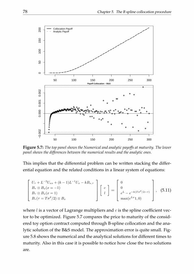
78 Chapter 5. The B spline collocation procedure
50 100 150 200 250 300
050
100
150
200
S
Collocation PayoffAnalytic Payoff
50 100 150 200 250 300
−0.
002
0.00
00.
001
0.00
2
Payoff Collocation − B&S
Figure 5.7: The top panel shows the Numerical and analytic payoffs at maturity. The lowerpanel shows the differences between the numerical results and the analytic ones.
This implies that the differential problem can be written stacking the differ-ential equation and the related conditions in a linear system of equations:
Uτ + L−2Uxx + (k − 1)L−1Ux − kBx,τ
Bτ ⊗Bx(x = −1)
Bτ ⊗Bx(x = 1)
Bτ (τ = Tσ2/2)⊗Bx
[ c
l
]=
0
0
eL − e−k(Tσ2/2−τ)
max(eLx1, 0)
, (5.11)
where l is a vector of Lagrange multipliers and c is the spline coefficient vec-tor to be optimized. Figure 5.7 compares the price to maturity of the consid-ered toy option contract computed through B-spline collocation and the ana-lytic solution of the B&S model. The approximation error is quite small. Fig-ure 5.8 shows the numerical and the analytical solutions for different times tomaturity. Also in this case it is possible to notice how close the two solutionsare.
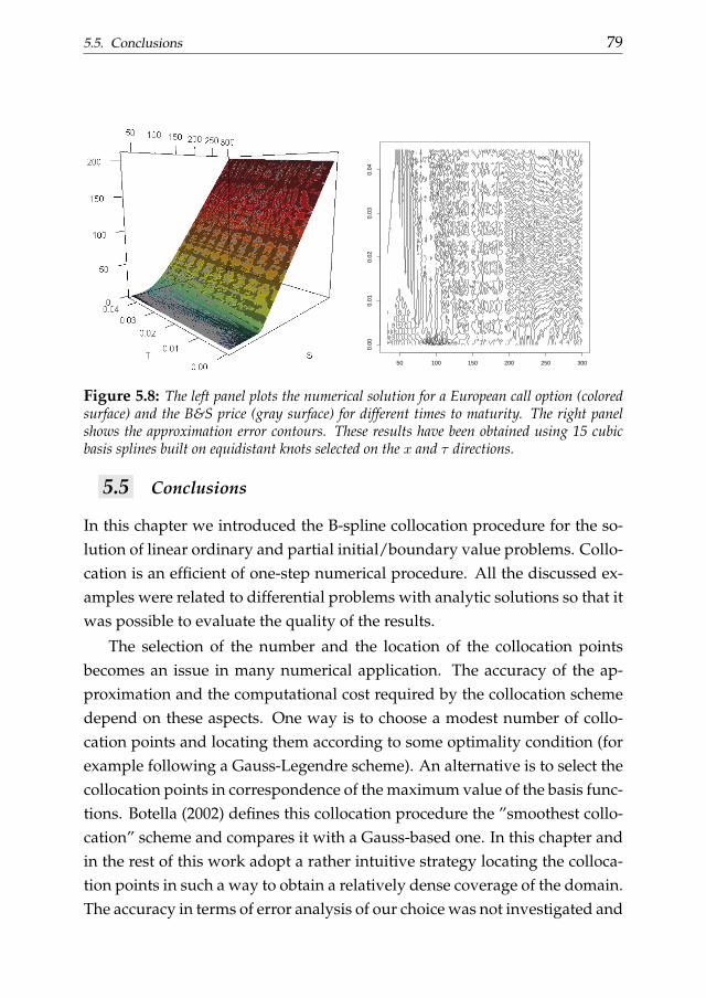
5.5. Conclusions 79
τ
−0.
005
0
0
0
0
0 0
0
0 0
0
0
0
0 0
0
0
0
0
0
0
0 0
0
0
0
0
0
0
0
0
0
0
0
0 0
0 0
0
0
0
0
0
0
0
0
0
0
0
0
0
0
0
0
0
0
0
0
0
0
0
0
0
0 0
0
0
0
0
0
0
0
0
0
0
0
0
0
0
0
0
0
0 0
0
0
0 0
0
0 0
0 0
0
0
0
0
0
0
0
0 0
0
0
0
0
0
0
0
0
0
0
0
0
0
0
0
0
0
0
0
0
0
0
0
0
0
0
0 0
0
0
0
0
0
0
0
0
0
0
0
0
0 0
0
0
0
0
0
0
0
0
0
0
0
0
0
0
0
0
0
0
0
0
0
0
0
0
0
0 0
0
0
0
0
0
0
0
0
0
0 0
0
0
0
0
0
0
0
0
0
0 0
0
0
0
0
0
0
0
0
0
0
0
0
0
0
0
0
0
0
0
0
0
0
0
0
0
0
0
0
0
0 0
0 0
0.0
05
50 100 150 200 250 3000.
000.
010.
020.
030.
04
Figure 5.8: The left panel plots the numerical solution for a European call option (coloredsurface) and the B&S price (gray surface) for different times to maturity. The right panelshows the approximation error contours. These results have been obtained using 15 cubicbasis splines built on equidistant knots selected on the x and τ directions.
5.5 Conclusions
In this chapter we introduced the B-spline collocation procedure for the so-lution of linear ordinary and partial initial/boundary value problems. Collo-cation is an efficient of one-step numerical procedure. All the discussed ex-amples were related to differential problems with analytic solutions so that itwas possible to evaluate the quality of the results.
The selection of the number and the location of the collocation pointsbecomes an issue in many numerical application. The accuracy of the ap-proximation and the computational cost required by the collocation schemedepend on these aspects. One way is to choose a modest number of collo-cation points and locating them according to some optimality condition (forexample following a Gauss-Legendre scheme). An alternative is to select thecollocation points in correspondence of the maximum value of the basis func-tions. Botella (2002) defines this collocation procedure the ”smoothest collo-cation” scheme and compares it with a Gauss-based one. In this chapter andin the rest of this work adopt a rather intuitive strategy locating the colloca-tion points in such a way to obtain a relatively dense coverage of the domain.The accuracy in terms of error analysis of our choice was not investigated and
80 Chapter 5. The B spline collocation procedure
will be part of our future research.As practical application we have shown how to solve the Black and Sc-
holes differential problem for pricing European options using a B-spline col-location procedure. A plain vanilla call option has been considered. Thenumerical approximation of the price to maturity has been compared withthe analytic solution of the B&S model. The same comparison has been per-formed computing the price of an analogous option contracts with differenttimes to maturity. In all the cases the price approximated by collocation hasbeen found really close to the price computed using the analytic solution ofthe differential problem.
Further generalizations of the collocation scheme are possible and will beillustrated in the coming chapters. We will show, for example, that it is possi-ble to define a collocation procedure able to take into account inequality con-straints imposed on the state function or on one (or more) of its derivative(s).Analogously, using a B-spline collocation procedure, it is possible to approx-imate state functions imposing irregularities on its domain or codomain. Fi-nally, the collocation approach is flexible enough to be adopted to approx-imate the solution of different classes of differential problems such as timevarying parameter, non linear and delayed equations.
DIFFERENTIAL PENALIZED SMOOTHING 6Smoothing procedures driven by differential equations have gained
popularity in the last few years. These methods combine basis functionsand differential operators in a penalized estimation setting. The results ofthe analysis are interpretable in relation to the dynamics described by thedifferential law taken into account. In this chapter we show an approachfor functional smoothing able to take into account not only the differen-tial operator but also initial/boundary conditions. We also propose a two-stage procedure based on P-splines for the estimation of the unknown DEparameters.Keywords: B-splines, collocation method, P-splines, Ordinary Differen-tial Equations, generalized conditions.
6.1 Introduction
Penalized smoothing techniques have a prominent place in modern over-parametric regression analysis. The penalty term determines the character-istics of the final fit, balancing between smoothness and fidelity to the dataof the estimated curves. In this chapter we formulate a penalized smoothingproblem based on B-spline functions guaranteeing a certain degree of flexi-bility to the final estimates.
Different definitions of the penalty term have been proposed in the liter-ature. Smoothing splines are based on a penalty term representing the inte-grated second derivative of the final fit. On the other hand penalized splines(P-splines), introduced by Eilers and Marx in 1996, define a penalty term ob-tained as differences between the spline coefficients.
More general penalties are possible. L-spline smoothing techniques con-sider penalty terms combining the derivatives of the final estimates defining
81
82 Chapter 6. Differential penalized smoothing
a differential operator. The idea is to smooth the raw data penalizing the leastsquares problem taking into account a model for the underlying dynamics.Examples of this kind of approach have been discussed by Schumaker (1981),Ramsay and Silverman (2005), Welham et al. (2006), Wood et al. (2008) andmany others. In this framework the observed data can be viewed as a sortof generalized conditions applied to a numerical scheme for the numericalsolution of a differential equation.
This approximation is obtained by balancing between two conflictingaims: the fidelity to the data (measured by the residual sum of squares) andthe fidelity to the approximate solution of the differential problem behindthem (obtained integrating the differential operator included in the penalty):
minc‖y − x(t, c)‖2 + λ
∫[L(x(t, c), w)]2dt,
where c is the vector of of basis coefficients determining the smoothing func-tion, L(x(t, c), w) is a differential operator that depends on the differentialparameters vector w and λ is a smoothing parameter determining the em-phasis given to the numerical scheme in the estimation procedure.
In practical applications the parameters w have to be estimated from theavailable observations. A possibility is to estimate them minimizing a jointpenalized log-likelihood. The penalized minimization problem can be sim-plified, exploiting the hierarchy existing between the unknowns and consid-ering the basis coefficients as nuisance parameters, leading to the so called”generalized profiling technique” proposed by Cao and Ramsay (2007).
In this chapter we propose to estimate the unknown DE parameters usinga P-spline-based two-stage approach moving from the consideration that, ifthe differential problem represents a good description of the observed mea-surements, the signal has to be consistent with the state function.
This chapter is organized as follows: in section 6.2 the differential pe-nalized smoothing approach is introduced in the case of known differentialoperators. We also discuss the introduction of known and unknown ini-tial/boundary conditions defining the differential problem clarifying the roleof Lagrange multipliers in the estimation procedure. In section 6.3 we focuson the role of the smoothing parameter introducing an EM-based algorithm(see Schall, 1991) for its optimization. In section 6.4 we deal with smooth-ing problems driven by unknown linear differential operators introducing

6.2. Smoothing with ordinary differential penalties 83
a P-spline-based two-stage approach to estimate the unknown DE parame-ters. The performance of this procedure is evaluated through two simulationstudies. Finally, in section 6.5, a real data example is analyzed.
6.2 Smoothing with ordinary differential penalties
Suppose we observe a set of noisy data described, at least approximatively,by a differential model and have an idea about the ODE describing the dy-namic underlying the observations What happens if our knowledge aboutthe differential equation describing the observed dynamics is not precise oreven not correct? In this case the solution of the differential problem wouldprovide an inadequate description of the observed measurements. It is pos-sible to overcome this problem forcing the solution of the DE we have inmind to give an appropriate description of the data. This can be achievedusing a smoothing approach penalized by a differential operator approxi-mated using a collocation scheme. If we define u(t) =
∑ni Bj(t)cj the ap-
proximated state function computed using a B-spline collocation procedureand V (w, t) =
∑nj
∑md=0wdB
(d)j cj the approximated differential operator, our
estimation problem is summarized by:
minc‖y −
n∑j
Bjcj‖2 + λ‖n∑j
m∑d=0
wdB(d)j cj‖2, (6.1)
where λ is a smoothing parameter balancing between the residual sum ofsquares and the collocation approximation of the observed dynamics, c is avector of unknown spline coefficients, w is a vector of m DE parameters thatwe consider, for the moment, known (m indicates the order of the differentialoperator that we consider to be linear in this chapter).
In the formulation above we used the breve accent to distinguish twosets of points on which the basis functions are evaluated. The B-splines in-volved in the penalty term are evaluated on an ”enlarged” set of N collo-cation points. On the other hand the basis functions in B are evaluated atobserved domain points. This definition of the penalty term is convenientin those cases a moderate number of observations is available providing amore precise definition of the collocation solution of the hypothesized differ-ential problem. This issue is particularly relevant when we are interested inestimating the DE parameters from the data, as we discuss later.
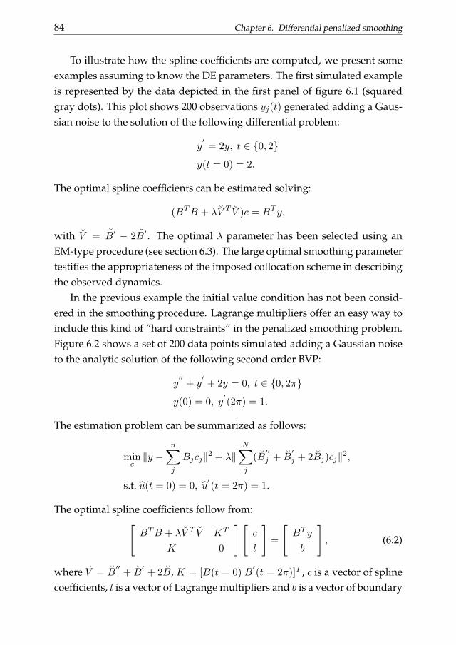
84 Chapter 6. Differential penalized smoothing
To illustrate how the spline coefficients are computed, we present someexamples assuming to know the DE parameters. The first simulated exampleis represented by the data depicted in the first panel of figure 6.1 (squaredgray dots). This plot shows 200 observations yj(t) generated adding a Gaus-sian noise to the solution of the following differential problem:
y′
= 2y, t ∈ 0, 2
y(t = 0) = 2.
The optimal spline coefficients can be estimated solving:
(BTB + λV T V )c = BT y,
with V = B′ − 2B′ . The optimal λ parameter has been selected using anEM-type procedure (see section 6.3). The large optimal smoothing parametertestifies the appropriateness of the imposed collocation scheme in describingthe observed dynamics.
In the previous example the initial value condition has not been consid-ered in the smoothing procedure. Lagrange multipliers offer an easy way toinclude this kind of ”hard constraints” in the penalized smoothing problem.Figure 6.2 shows a set of 200 data points simulated adding a Gaussian noiseto the analytic solution of the following second order BVP:
y′′
+ y′+ 2y = 0, t ∈ 0, 2π
y(0) = 0, y′(2π) = 1.
The estimation problem can be summarized as follows:
minc‖y −
n∑j
Bjcj‖2 + λ‖N∑j
(B′′j + B
′j + 2Bj)cj‖2,
s.t. u(t = 0) = 0, u′(t = 2π) = 1.
The optimal spline coefficients follow from:[BTB + λV T V KT
K 0
][c
l
]=
[BT y
b
], (6.2)
where V = B′′
+ B′+ 2B, K = [B(t = 0) B
′(t = 2π)]T , c is a vector of spline
coefficients, l is a vector of Lagrange multipliers and b is a vector of boundary
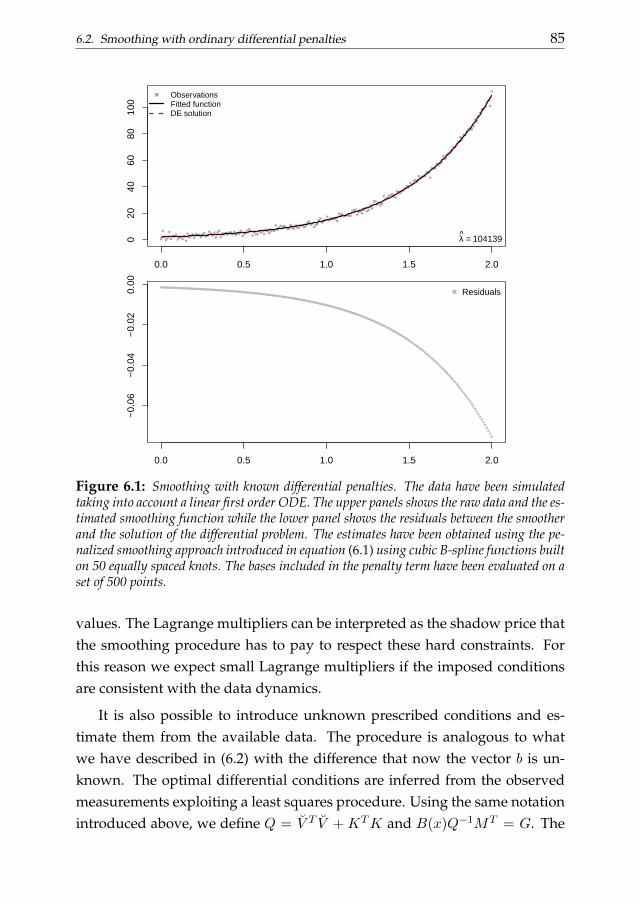
6.2. Smoothing with ordinary differential penalties 85
0.0 0.5 1.0 1.5 2.0
020
4060
8010
0
x
ObservationsFitted functionDE solution
λ = 104139
0.0 0.5 1.0 1.5 2.0
−0.
06−
0.04
−0.
020.
00
Residuals
Figure 6.1: Smoothing with known differential penalties. The data have been simulatedtaking into account a linear first order ODE. The upper panels shows the raw data and the es-timated smoothing function while the lower panel shows the residuals between the smootherand the solution of the differential problem. The estimates have been obtained using the pe-nalized smoothing approach introduced in equation (6.1) using cubic B-spline functions builton 50 equally spaced knots. The bases included in the penalty term have been evaluated on aset of 500 points.
values. The Lagrange multipliers can be interpreted as the shadow price thatthe smoothing procedure has to pay to respect these hard constraints. Forthis reason we expect small Lagrange multipliers if the imposed conditionsare consistent with the data dynamics.
It is also possible to introduce unknown prescribed conditions and es-timate them from the available data. The procedure is analogous to whatwe have described in (6.2) with the difference that now the vector b is un-known. The optimal differential conditions are inferred from the observedmeasurements exploiting a least squares procedure. Using the same notationintroduced above, we define Q = V T V + KTK and B(x)Q−1MT = G. The

86 Chapter 6. Differential penalized smoothing
0 1 2 3 4 5 6
−10
−5
05
x
ObservationsFitted functionDE solutionBoundary condition
λ = 6661
l 1 = 0.016
0 1 2 3 4 5 6
−30
−20
−10
010
x
Approximated first derivativeBoundary condition
l 2 = 0.069
0 1 2 3 4 5 6
−0.
0025
−0.
0015
−0.
0005
0.00
05 Residuals
Figure 6.2: Smoothing with known differential penalties and boundary conditions. Thedata have been simulated taking into account a linear second order ODE. The upper panelsshows the raw data and the estimated smoothing function while the lower panel shows theresiduals between the smoother and the solution of the differential problem. These estimateshave been obtained considering 50 cubic spline functions built on equally spaced knots. Thebases involved in the penalty term have been evaluated on a grid of 500 domain points.
optimal prescribed values follow from:
(GTG)b = GT y.
Once that these values have been estimated they can be plugged in (6.2) tofind the spline coefficients minimizing the constrained penalized smoothingproblem.
Figure 6.3 shows the results obtained smoothing a series of data describedby the system of ODEs:
x′1 = x2
x′2 = −x1 − 0.5x2
s.t. x1(0) = 0, x2(0) = 2
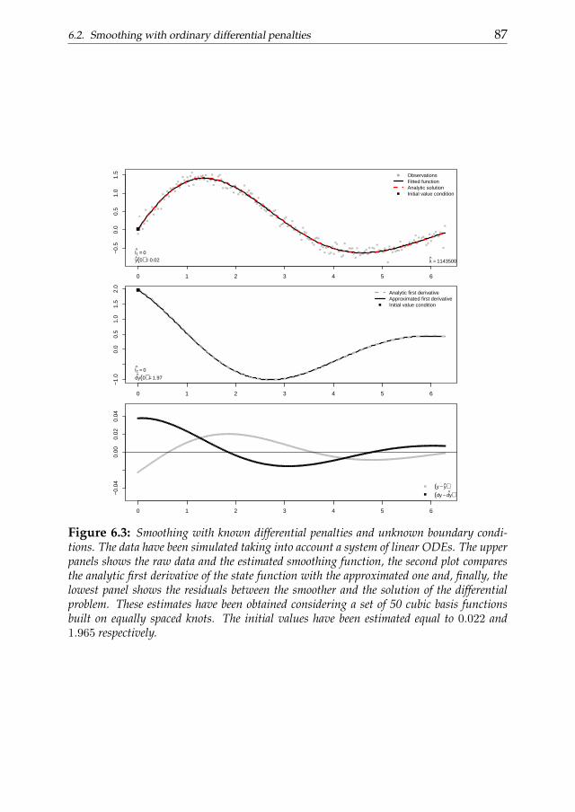
6.2. Smoothing with ordinary differential penalties 87
0 1 2 3 4 5 6
−0.
50.
00.
51.
01.
5
x
ObservationsFitted functionAnalytic solutionInitial value condition
λ = 1143500
l1^ = 0
y(0) = 0.02
0 1 2 3 4 5 6
−1.
00.
00.
51.
01.
52.
0
x
Analytic first derivativeApproximated first derivativeInitial value condition
l2^ = 0
dy(0) = 1.97
0 1 2 3 4 5 6
−0.
040.
000.
020.
04
(y − y)(dy − dy)
Figure 6.3: Smoothing with known differential penalties and unknown boundary condi-tions. The data have been simulated taking into account a system of linear ODEs. The upperpanels shows the raw data and the estimated smoothing function, the second plot comparesthe analytic first derivative of the state function with the approximated one and, finally, thelowest panel shows the residuals between the smoother and the solution of the differentialproblem. These estimates have been obtained considering a set of 50 cubic basis functionsbuilt on equally spaced knots. The initial values have been estimated equal to 0.022 and1.965 respectively.
88 Chapter 6. Differential penalized smoothing
The high value of the optimal smoothing parameter (selected again throughan EM-type algorithm) testifies that the differential problem penalizing thesmoothing procedure is appropriate to describe the observed dynamics. Thesame aspect can be evaluated considering the residuals between the analyticsolution and the smoothing function plotted in the lowest panel of the figure.
6.3 The role of the smoothing parameter
The smoothing parameter λ plays a crucial role in the evaluation of the ap-propriateness of the differential operator included in the penalty term. Thisparameter sets the balance between to the data and the fidelity to the DE.
For λ→∞ fidelity to the DE becomes all-important and the data provideonly generalized boundary conditions. On the other hand when λ → 0 weget a B-spline fit which may lead to trouble because support might be missingfor some basis functions.
It is attractive to use the data to set an appropriate value of λ. In principle,all the automatic selection criteria introduced in chapter 3 can be used. Herewe introduce a different procedure based on an EM-type algorithm that willbe crucial for the mixed model framework we will present in the next chapter.
This algorithm was originally proposed by Schall (1991) as an iterativeestimation procedure for mixed effects and dispersion components in gener-alized linear models with random effects (mixed models). This approachmoves from the formal equivalence between penalized least squares andmixed models (we will discuss this topic in more details in the next chap-ter). The same equivalence can be exploited to select the optimal smoothingparameter.
The optimization algorithm consists of two alternating steps. In the firststep the optimal spline coefficients are estimated considering a given value ofλ. In a second step the variance components of the errors (σ2
ε ) and the penaltyvariance (σ2
p) are estimated. Then the value of the smoothing parameter isupdated taking it equal to the ratio between the current estimates of thesevariances: λ = σ2
ε /σ2p . The procedure is iterated until convergence of the
smoothing parameter.
The two variance components are functions of the effective model dimen-

6.4. Smoothing with unknown differential penalties 89
0.0 0.5 1.0 1.5 2.0
020
4060
8010
0
1y' −2y=0
x
λ = 1820.88
ObservationsSmoother
0.0 0.5 1.0 1.5 2.0
020
4060
8010
0
−1y' −2y=0
λ = 1.9e−05
ObservationsSmoother
Figure 6.4: smoothing data described by a linear first order ODE (exponential growth).Each plot shows the results obtained for different DE parameters. In the legend of each panelthe optimal smoothing parameter is indicated.
sion ED = tr[B(BTB + λV T V )−1BT ]:
σ2ε = ‖y−Bc‖2
n−ED
σ2p = ‖V (w)c‖2
ED
(6.3)
Figure 6.4 clarifies the impact of the parameters of the DE on the optimalvalue of λ selected through an EM-algorithm. If the penalty is close to the DEthe optimal λ is large; otherwise it is small.
6.4 Smoothing with unknown differential penalties
It is possible to estimate the unknown DE parameters. A common approachis to write the (analytic or numerical) solution of the equation as explicit func-tion of the unknown parameters to be estimated from the data. This generally

90 Chapter 6. Differential penalized smoothing
leads to a nonlinear regression problem even if the DE is linear. An alter-native approach is to incorporate the differential equation as a penalty in asmoothing framework as suggested by Ramsay and Silverman (2005). Theoptimal DE parameters and smoothing coefficients are then estimated min-imizing the penalized joint log-likelihood. A more convenient estimationprocedure exploiting a generalized profiling likelihood criterion has beenproposed by Cao and Ramsay (2007). Here we propose a two-stage P-spline-based estimation of the unknown DE parameters.
We start from the consideration that the state function solving the DEdescribing the observed will be consistent with the data signal if the DE isappropriate. First the signal is extracted from the noisy measurements usinga P-spline smoother. The optimal amount of smoothing is determined by theEM-algorithm. The estimated spline coefficients are then used to estimate theparameter vector w through least squares.
Once the differential parameters have been estimated we define thepenalty term V and use it to estimate the optimal spline coefficients:
c = (BTB + λV T V )−1BT y. (6.4)
Figure 6.5 shows an example based on 200 observations generated takinginto account the analytic solution of following the system of first order ODEs:
x′1 = x2
x′2 = −x1 − 1
2x2
x1(0) = 0; x2(0) = 2.
6.4.1 Simulations
We propose two simulation studies related to a first and a second order DE.We want to evaluate the influence of the sample size, the number of subjectsand the variance of the noise component on the estimates.
The first order differential problem that we take into account is:
y′
= y
y(0) = 2.
This IVP has analytic solution y∗(t) = 2 exp(−x). We perform our simula-tions for 4 different sample sizes: N = 20, 50, 100, 200 and 4 noise standard
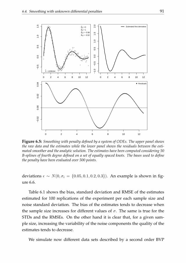
6.4. Smoothing with unknown differential penalties 91
0 2 4 6 8 10 12
−0.
50.
00.
51.
01.
5
x
λ = 1208164
w1 = 0w2 = 1w3 = −0.98
w4 = −0.52
0 2 4 6 8 10 12
−1.
0−
0.5
0.0
0.5
1.0
1.5
2.0
x
(KB
1 %
*% a
)[1:
200]
Estimated first derivative
0 2 4 6 8 10 12
−0.
020.
000.
020.
04 Residuals
Figure 6.5: Smoothing with penalty defined by a system of ODEs. The upper panel showsthe raw data and the estimates while the lower panel shows the residuals between the esti-mated smoother and the analytic solution. The estimates have been computed considering 50B-splines of fourth degree defined on a set of equally spaced knots. The bases used to definethe penalty have been evaluated over 500 points.
deviations ε ∼ N(0, σi = 0.05, 0.1, 0.2, 0.3). An example is shown in fig-ure 6.6.
Table 6.1 shows the bias, standard deviation and RMSE of the estimatesestimated for 100 replications of the experiment per each sample size andnoise standard deviation. The bias of the estimates tends to decrease whenthe sample size increases for different values of σ. The same is true for theSTDs and the RMSEs. On the other hand it is clear that, for a given sam-ple size, increasing the variability of the noise components the quality of theestimates tends to decrease.
We simulate now different data sets described by a second order BVP
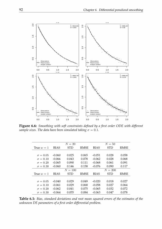
92 Chapter 6. Differential penalized smoothing
0.0 0.5 1.0 1.5 2.0
0.5
1.0
1.5
2.0
N = 20
x
λ = 8534.635w = 0.964
ObservationsFitted functionAnalytic soluiton
0.0 0.5 1.0 1.5 2.0
0.5
1.0
1.5
2.0
N = 50
xy
λ = 9996.457w = 0.98
ObservationsFitted functionAnalytic soluiton
0.0 0.5 1.0 1.5 2.0
0.5
1.0
1.5
2.0
N = 100
λ = 9999.766w = 0.983
ObservationsFitted functionAnalytic soluiton
0.0 0.5 1.0 1.5 2.0
0.5
1.0
1.5
2.0
N = 200
yλ = 9999.937w = 0.978
ObservationsFitted functionAnalytic soluiton
Figure 6.6: Smoothing with soft constraints defined by a first order ODE with differentsample sizes. The data have been simulated taking σ = 0.1.
N = 20 N = 50True w = 1 BIAS STD RMSE BIAS STD RMSE
σ = 0.05 -0.060 0.025 0.065 -0.051 0.028 0.058σ = 0.10 -0.066 0.043 0.078 -0.062 0.028 0.068σ = 0.20 -0.065 0.090 0.111 -0.068 0.061 0.091σ = 0.30 -0.060 0.146 0.158 -0.076 0.090 0.117
N = 100 N = 200True w = 1 BIAS STD RMSE BIAS STD RMSE
σ = 0.05 -0.040 0.029 0.049 -0.020 0.018 0.027σ = 0.10 -0.061 0.029 0.068 -0.058 0.027 0.064σ = 0.20 -0.062 0.041 0.075 -0.065 0.032 0.072σ = 0.30 -0.064 0.055 0.084 -0.063 0.047 0.078
Table 6.1: Bias, standard deviations and root mean squared errors of the estimates of theunknown DE parameters of a first order differential problem.

6.4. Smoothing with unknown differential penalties 93
0 1 2 3 4 5
−1.
5−
1.0
−0.
50.
00.
51.
01.
5
N = 20
x
λ = 287.748w1 = 8.902w2 = −0.02
ObservationsFitted functionAnalytic soluiton
0 1 2 3 4 5
−1.
5−
1.0
−0.
50.
00.
51.
01.
5
N = 50
x
y
λ = 419.879w1 = 9.086w2 = 0.016
ObservationsFitted functionAnalytic soluiton
0 1 2 3 4 5
−1.
5−
1.0
−0.
50.
00.
51.
01.
5
N = 100
λ = 591.575w1 = 9.181w2 = 0.054
ObservationsFitted functionAnalytic soluiton
0 1 2 3 4 5
−1.
5−
0.5
0.0
0.5
1.0
1.5
N = 200
y
λ = 581.898w1 = 9.196w2 = 0.008
ObservationsFitted functionAnalytic soluiton
Figure 6.7: Smoothing with soft constraints defined by a second order order ODE withdifferent sample sizes.
(harmonic oscillatory system):
y′′
+ 9y = 0
y(0) = 0, y(5) = 1.
Figure 6.7 shows the estimates obtained generating noisy data of 4 samplesizes from the analytic solution of this BVP: y∗(t) = sin(3t)/ sin(15). The er-ror component was considered normally distributed with standard deviationequal to 0.1.
For the simulations we used the same settings discussed in the previ-ous example and the same number of replications. The results are shownin table 6.2. An increasing sample size tends to guarantee more precise, lessvariable and more robust estimates. Also the amount of variability of theerror component has an impact on the quality of the final estimates. As weexpected, for a given sample size the robustness, the variability and the pre-
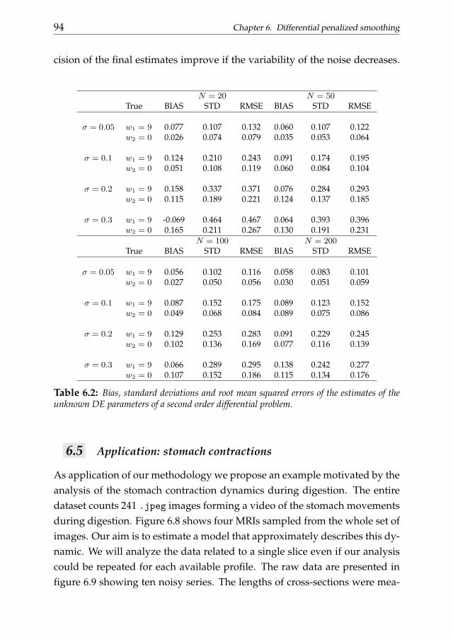
94 Chapter 6. Differential penalized smoothing
cision of the final estimates improve if the variability of the noise decreases.
N = 20 N = 50True BIAS STD RMSE BIAS STD RMSE
σ = 0.05 w1 = 9 0.077 0.107 0.132 0.060 0.107 0.122w2 = 0 0.026 0.074 0.079 0.035 0.053 0.064
σ = 0.1 w1 = 9 0.124 0.210 0.243 0.091 0.174 0.195w2 = 0 0.051 0.108 0.119 0.060 0.084 0.104
σ = 0.2 w1 = 9 0.158 0.337 0.371 0.076 0.284 0.293w2 = 0 0.115 0.189 0.221 0.124 0.137 0.185
σ = 0.3 w1 = 9 -0.069 0.464 0.467 0.064 0.393 0.396w2 = 0 0.165 0.211 0.267 0.130 0.191 0.231
N = 100 N = 200True BIAS STD RMSE BIAS STD RMSE
σ = 0.05 w1 = 9 0.056 0.102 0.116 0.058 0.083 0.101w2 = 0 0.027 0.050 0.056 0.030 0.051 0.059
σ = 0.1 w1 = 9 0.087 0.152 0.175 0.089 0.123 0.152w2 = 0 0.049 0.068 0.084 0.089 0.075 0.086
σ = 0.2 w1 = 9 0.129 0.253 0.283 0.091 0.229 0.245w2 = 0 0.102 0.136 0.169 0.077 0.116 0.139
σ = 0.3 w1 = 9 0.066 0.289 0.295 0.138 0.242 0.277w2 = 0 0.107 0.152 0.186 0.115 0.134 0.176
Table 6.2: Bias, standard deviations and root mean squared errors of the estimates of theunknown DE parameters of a second order differential problem.
6.5 Application: stomach contractions
As application of our methodology we propose an example motivated by theanalysis of the stomach contraction dynamics during digestion. The entiredataset counts 241 .jpeg images forming a video of the stomach movementsduring digestion. Figure 6.8 shows four MRIs sampled from the whole set ofimages. Our aim is to estimate a model that approximately describes this dy-namic. We will analyze the data related to a single slice even if our analysiscould be repeated for each available profile. The raw data are presented infigure 6.9 showing ten noisy series. The lengths of cross-sections were mea-
6.5. Application: stomach contractions 95
sured at 10 positions along the stomach, at each point in time. This gives 10time series of 300 measurements showing a rather oscillatory behavior. Wetake into account the dynamics described by the linear second order ODE:
y′′
+ w1y′+ w2y = 0.
This model is really simple but gives us the possibility to evaluate two impor-tant characteristics of the observed data: the period (π) of the oscillations andthe damping factor (ζ) associated to them. These characteristics are definedby the free response of the system, defined by the DE. It is a damped cosinefunction. The period is two times the distance between zero crossings. Thedamping is the ratio of two peaks separated by one period. The period of os-cillation is the smallest interval of time in which an oscillating system returnsto the sate it was at a time arbitrarily chosen. If the amplitude of the oscilla-tions decreases in time the system is defined ”damped”. Damping effects areusually induced by frictional forces and are measured by the damping ratio.The damping ratio is the dimensionless measure describing how oscillationsdecay after that a source of disturbance is applied. These quantities can beexpressed in terms of the DE parameters (w1 and w2) and are computed asfollows:
π = 2π
√1
w2; ζ =
w2
2√w1.
The solid lines in figure 6.9 depict the final estimates obtained using thepenalized smoothing procedure described above. The optimal smoothingparameters have been selected through an EM-type algorithm. The estimatedDE coefficients and the smoothing parameters per each curve are shown intable 6.3 and in the legends of each panel of figure 6.9.
From table 6.3 we deduce some information about the models that havebeen estimated per each profile. The optimal λ parameters are high for fewwaves showing a large period and are relatively small for the rest of thecases. Small smoothing parameters indicate low congruence of the data withthe imposed differential penalty. This seems reasonable looking at the data.It is evident from the smoothing curves that the oscillatory behavior of thedata presents an asymmetric pattern: the peaks are sharper than the valleys.This asymmetry is not consistent with the linear differential model used aspenalty in the smoothing procedure. Probably a nonlinear equation would
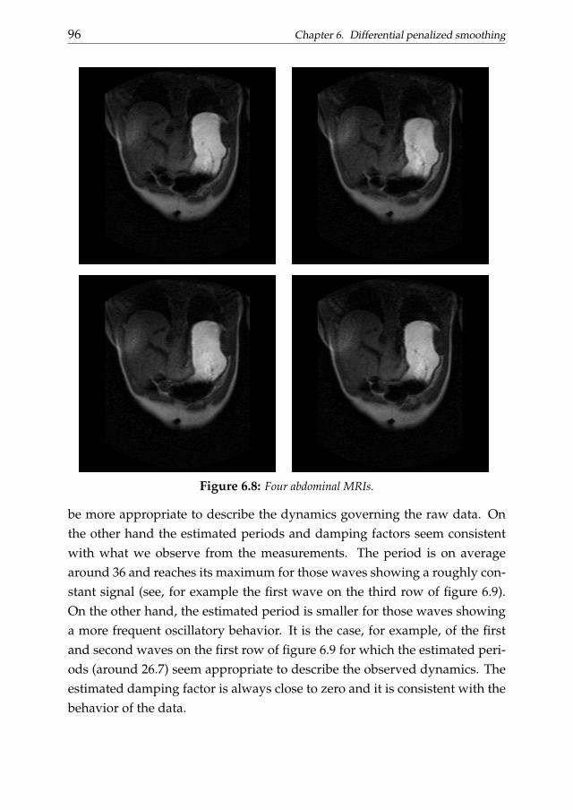
96 Chapter 6. Differential penalized smoothing
Figure 6.8: Four abdominal MRIs.
be more appropriate to describe the dynamics governing the raw data. Onthe other hand the estimated periods and damping factors seem consistentwith what we observe from the measurements. The period is on averagearound 36 and reaches its maximum for those waves showing a roughly con-stant signal (see, for example the first wave on the third row of figure 6.9).On the other hand, the estimated period is smaller for those waves showinga more frequent oscillatory behavior. It is the case, for example, of the firstand second waves on the first row of figure 6.9 for which the estimated peri-ods (around 26.7) seem appropriate to describe the observed dynamics. Theestimated damping factor is always close to zero and it is consistent with thebehavior of the data.

6.5. Application: stomach contractions 97
0 50 100 150 200 250 300
−2
02
4
x
λ = 8.751 w1 = 0.055
w2 = 0
0 50 100 150 200 250 300
−2
02
4
x
y
λ = 17.168 w1 = 0.055
w2 = −0.001
0 50 100 150 200 250 300
−2
02
4
x
λ = 247.476 w1 = 0.024
w2 = 0.012
0 50 100 150 200 250 300
−2
02
4
x
y
λ = 266.28 w1 = 0.031
w2 = 0.015
0 50 100 150 200 250 300
−2
02
4
x
λ = 1153.892 w1 = 0.012
w2 = 0.015
0 50 100 150 200 250 300−
20
24
x
y
λ = 31.056 w1 = 0.023
w2 = 0
0 50 100 150 200 250 300
−2
02
4
x
λ = 32.735 w1 = 0.026
w2 = 0.02
0 50 100 150 200 250 300
−2
02
4
x
y
λ = 121.653 w1 = 0.042
w2 = 0.004
0 50 100 150 200 250 300
−2
02
4 λ = 111.592 w1 = 0.044
w2 = 0.005
0 50 100 150 200 250 300
−2
02
4
y
λ = 31.04 w1 = 0.035
w2 = 0.005
Figure 6.9: Smoothing of 10 stomach profiles. The black lines represent the estimatesobtained with the procedure described above. The estimated DE coefficients, the smoothingparameters and the Lagrange multipliers are shown in the legend of each plot. The estimateshave been obtained using 100 fourth order B-splines built on equally spaced knots. The basesdefining the penalty term have been evaluated over 500 domain points.
Wave w1 w2 λ π ζ
1 0.055 0.001 8.7 26.7 0.0012 0.055 -0.001 17.2 26.7 -0.0023 0.024 0.012 247.5 40.4 0.0374 0.031 0.015 266.3 35.5 0.0435 0.012 0.015 1153.9 57.5 0.0696 0.023 0.001 31.1 41.3 -0.0017 0.026 0.020 32.7 39.1 0.0618 0.042 0.004 121.6 30.6 0.0109 0.044 0.005 111.6 29.9 0.011
10 0.035 0.005 31.0 33.5 0.013
Table 6.3: Estimated DE components and optimal λ for each stomach wave.
98 Chapter 6. Differential penalized smoothing
6.6 Conclusions
In this chapter we introduced an ODE-based penalized smoothing approachusing a linear combination of basis spline functions for the approximationof the state function in analogy with a B-spline collocation scheme. Penal-izing the smoothing procedure by a linear differential operator we imposedconsistency between the estimated smoothing function and the state functionapproximating the solution of the ODE-based penalty.
A smoothing parameter (λ) regulates the fidelity of the final estimatesto the DE. This parameter, if selected using an automatic procedure, can beinterpreted as a data-based measure of the appropriateness of the differen-tial operator penalty. We suggested to select this parameter through an EM-type algorithm exploiting the mixed model interpretation of penalized leastsquares.
Initially we have supposed to know exactly the form of the DE governingthe observed dynamics. This is an unrealistic hypothesis in real data anal-yses. For this reason we introduced a two-stage P-spline-based procedureto estimate the unknown DE parameters, parameters following these steps:1) smooth the raw data using a P-spline smoother able to separate the datatrend from the noise component, 2) estimate the unknown DE parametersfrom the fitted curve through least squares. This simplifies, in our opinion,the estimation task separating the computation of the DE parameters fromthe data smoothing problem. The performances of this approach have beenevaluated through simulations.
We also analyzed a real data example based on a set of time series describ-ing the contraction movements of a stomach cross-section extracted fromMRI images. A second order linear differential model has been proposedto describe this dynamics. The estimated differential parameters seem con-sistent with the data evidence even if the proposed linear differential modelappears too simple to describe the observed asymmetric oscillatory behav-ior. A nonlinear differential equation should give more appropriate resultsbut we did not evaluate yet the possibility to generalize our approach to non-linear differential equations.
Further generalizations are possible. First of all, it is possible to allow formixed effect DE parameters (we will discuss this topic in the next chapter).
6.6. Conclusions 99
This generalization is useful when the available observations are groupedaccording to some factor. On the other hand, it is possible to extend the pro-posed procedure to smooth data representing system dynamics evolving inmore than one dimension combining tensor product smoothing splines andpartial differential penalties.


DIFFERENTIAL OPERATOR PENALTIES WITH
MIXED PARAMETERS 7Smoothing techniques able to take into account the dynamics of sys-
tems described by differential problems have been proposed in the literatureby many authors. Most of these approaches consider the unknown differ-ential parameters as fixed effects. In many applications it is interesting tostudy the relationship between measurements grouped according to one ormore factors. This leads to a mixed model formulation. In this chapter wepropose an ODE-based penalized smoothing spline approach to analyzethe measurements of dynamic systems described by differential equationswith mixed parameters.Keywords: Penalized least squares, smoothing splines, random effects,differential problems.
7.1 Introduction
Differential equations (DEs) are powerful tools for describing dynamic sys-tems. In practical applications the values of their parameters have to be es-timated from observed data. The common approach is to write the solutionof the equation as an explicit function of the parameters and fit them to thedata. Generally this leads to a nonlinear regression problem even if the DEsare linear. If no explicit solution is available a similar approach can be usedbased on numerical solution of the DE.
An alternative is to incorporate the differential equation as a penalty ina smoothing framework (Ramsay and Silverman, 2005). In this case a jointpenalized log-likelihood has to be minimized in order to estimate a smoothversion of the raw data together with the unknown DE parameters. The pe-nalized minimization problem can be simplified exploiting the hierarchy ex-isting between the unknowns and considering the basis coefficients as nui-
101
102 Chapter 7. Differential operator penalties with mixed parameters
sance parameters. This leads to the so called generalized profiling techniqueproposed by Cao and Ramsay (2007). In the previous chapter we have pro-posed an alternative P-spline-based two stage procedure.
In many data analyses the data are grouped in some way. Typical ex-amples are measurements on different subjects or collected repeatedly overtime. A mixed model is a natural way to analyze grouped data. In the caseof dynamic systems it would be a mixed model for the DE parameters.
A classical procedure for the estimation of a random and a fixed com-ponent of the DE parameters involves a nonlinear mixed model approach.Given the analytic or numerical solution of the DE, the related parameterscan be estimated using nonlinear mixed models. This is the rationale behindmany well known software packages like NONMEM and MONOLIX.
An alternative is a semiparametric approach including the DE in asmoothing framework as a penalty term. The mixed DE parameters are thenestimated minimizing the penalized joint log-likelihood or a restricted likeli-hood function. A generalized profiling approach to solve this estimation taskhas been proposed by Wang et al. (2012).
In this chapter we extend our discussion about differential penalizedsmoothing allowing for a mixed model formulation of the differential pa-rameters. We propose to adopt a P-spline-based two-stage procedure for theestimation of the fixed and random components, exploiting the link betweenpenalized regression and mixed model framework, in order to estimate theresidual and random effects variance components (Pawitan, 2001).
This chapter is organized as follows: in section 7.2 the relationship be-tween penalized least squares and mixed models is reviewed; in section 7.3we introduce the two-stage procedure for the estimation of mixed DE param-eters analyzing a simulated example; in section 7.4 two simulation studies arediscussed in order to evaluate the performance of our proposals while in sec-tion 7.6 our approach is used to analyze the stomach MRI data introduced inthe previous chapter.
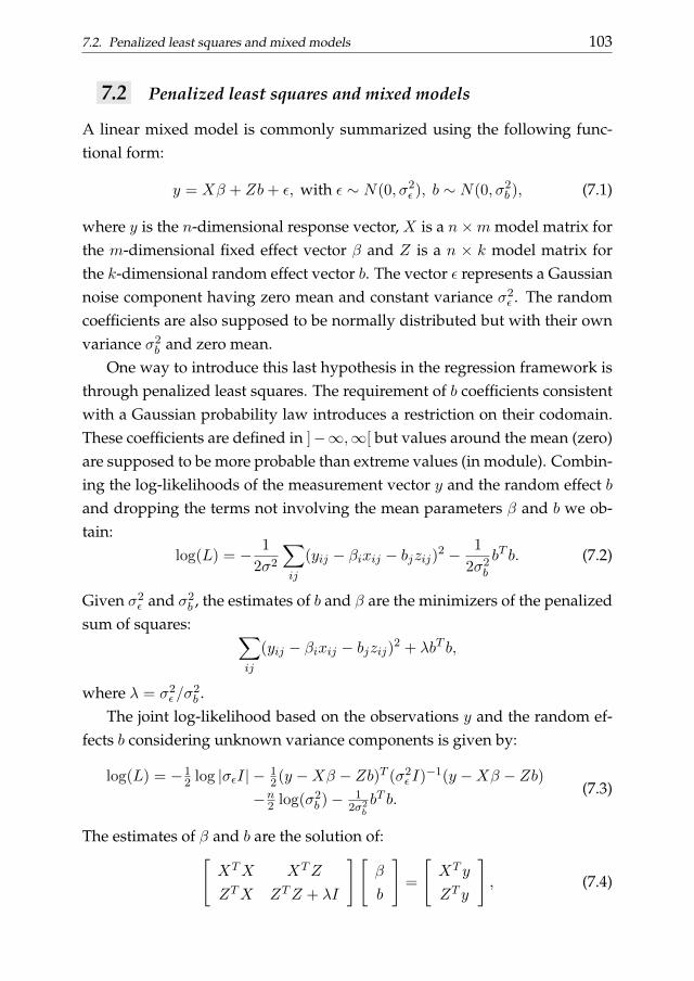
7.2. Penalized least squares and mixed models 103
7.2 Penalized least squares and mixed models
A linear mixed model is commonly summarized using the following func-tional form:
y = Xβ + Zb+ ε, with ε ∼ N(0, σ2ε ), b ∼ N(0, σ2
b ), (7.1)
where y is the n-dimensional response vector, X is a n×m model matrix forthe m-dimensional fixed effect vector β and Z is a n × k model matrix forthe k-dimensional random effect vector b. The vector ε represents a Gaussiannoise component having zero mean and constant variance σ2
ε . The randomcoefficients are also supposed to be normally distributed but with their ownvariance σ2
b and zero mean.One way to introduce this last hypothesis in the regression framework is
through penalized least squares. The requirement of b coefficients consistentwith a Gaussian probability law introduces a restriction on their codomain.These coefficients are defined in ]−∞,∞[ but values around the mean (zero)are supposed to be more probable than extreme values (in module). Combin-ing the log-likelihoods of the measurement vector y and the random effect band dropping the terms not involving the mean parameters β and b we ob-tain:
log(L) = − 1
2σ2
∑ij
(yij − βixij − bjzij)2 − 1
2σ2b
bT b. (7.2)
Given σ2ε and σ2
b , the estimates of b and β are the minimizers of the penalizedsum of squares: ∑
ij
(yij − βixij − bjzij)2 + λbT b,
where λ = σ2ε /σ
2b .
The joint log-likelihood based on the observations y and the random ef-fects b considering unknown variance components is given by:
log(L) = −12 log |σεI| − 1
2(y −Xβ − Zb)T (σ2ε I)−1(y −Xβ − Zb)
−n2 log(σ2
b )−1
2σ2bbT b.
(7.3)
The estimates of β and b are the solution of:[XTX XTZ
ZTX ZTZ + λI
][β
b
]=
[XT y
ZT y
], (7.4)
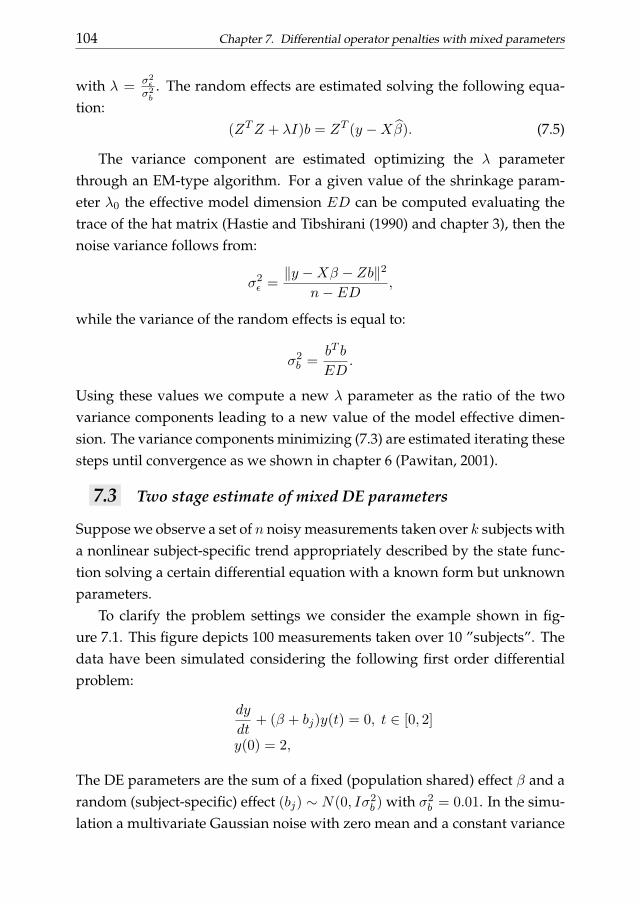
104 Chapter 7. Differential operator penalties with mixed parameters
with λ = σ2ε
σ2b
. The random effects are estimated solving the following equa-tion:
(ZTZ + λI)b = ZT (y −Xβ). (7.5)
The variance component are estimated optimizing the λ parameterthrough an EM-type algorithm. For a given value of the shrinkage param-eter λ0 the effective model dimension ED can be computed evaluating thetrace of the hat matrix (Hastie and Tibshirani (1990) and chapter 3), then thenoise variance follows from:
σ2ε =‖y −Xβ − Zb‖2
n− ED,
while the variance of the random effects is equal to:
σ2b =
bT b
ED.
Using these values we compute a new λ parameter as the ratio of the twovariance components leading to a new value of the model effective dimen-sion. The variance components minimizing (7.3) are estimated iterating thesesteps until convergence as we shown in chapter 6 (Pawitan, 2001).
7.3 Two stage estimate of mixed DE parameters
Suppose we observe a set of n noisy measurements taken over k subjects witha nonlinear subject-specific trend appropriately described by the state func-tion solving a certain differential equation with a known form but unknownparameters.
To clarify the problem settings we consider the example shown in fig-ure 7.1. This figure depicts 100 measurements taken over 10 ”subjects”. Thedata have been simulated considering the following first order differentialproblem:
dy
dt+ (β + bj)y(t) = 0, t ∈ [0, 2]
y(0) = 2,
The DE parameters are the sum of a fixed (population shared) effect β and arandom (subject-specific) effect (bj) ∼ N(0, Iσ2
b ) with σ2b = 0.01. In the simu-
lation a multivariate Gaussian noise with zero mean and a constant variance

7.3. Two stage estimate of mixed DE parameters 105
equal to 0.07 has been added to the numerical solution of the differentialmodel. The fixed effects have been considered equal to β1 = 1.
Our aim is to estimate the unknown fixed and random DE parametersstarting from the subject specific measurements. We propose a two-stageapproach to get these estimates. We suggest to proceed as follows: 1) fit a P-spline smoother for each subject specific measurement set such that to sepa-rate the trend component from the random noise, 2) use the estimated penal-ized spline coefficients to approximate the state function and its derivatives.The unknown mixed DE and the variance components are estimated througha linear mixed model approach. These estimates can be conveniently ob-tained exploiting the relationship between LMM and penalized least squaresdiscussed above.
For the example that we are considering the linear model to be estimatedis:
y = Xβ + Zb+ ε, ε ∼ N(0, σ2ε I), b ∼ N(0, σ2
b I),
with y a (1000× 1) vector of y′
estimated over all the subjects, X a (1000× 1)
matrix containing y estimated for each subject and Z a (1000×10) block diag-onal matrix with each block representing the approximated subject-specificy:
Z =
Z1 0 · · · 0
0 Z2 · · · 0...
. . . . . ....
0 · · · · · · Zm
.The fixed and random effects are estimated solving:[
XTX XTZ
ZTX ZTZ + λI
][β
b
]=
[XT y
ZT y
].
The estimates of the random coefficients depend on the value of the shrink-age parameter. In the mean time this parameter is used to estimate the vari-ance of the random effect. These unknowns are estimated together optimiz-ing the value of λ through an EM-algorithm in analogy with what we dis-cussed in the previous section. On the other hand the error variance cannotbe estimated in this step given that we are using a smooth version of the datato approximate the DE parameters. This variance component is obtained in
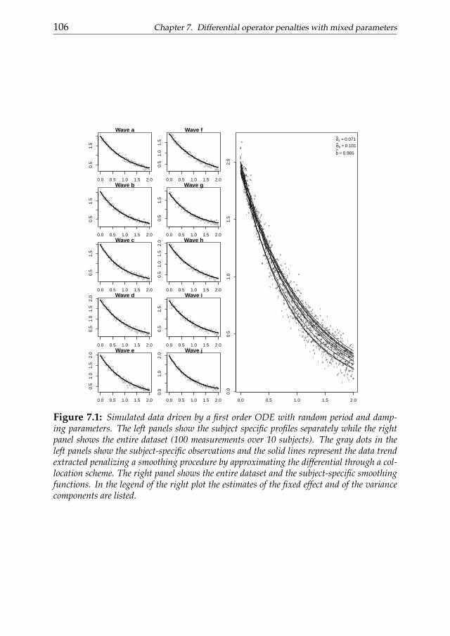
106 Chapter 7. Differential operator penalties with mixed parameters
0.0 0.5 1.0 1.5 2.0
0.5
1.5
Wave a
x
0.0 0.5 1.0 1.5 2.0
0.5
1.5
Wave b
x
0.0 0.5 1.0 1.5 2.0
0.5
1.5
Wave c
x
0.0 0.5 1.0 1.5 2.0
0.5
1.0
1.5
2.0 Wave d
x
0.0 0.5 1.0 1.5 2.0
0.5
1.0
1.5
2.0 Wave e
0.0 0.5 1.0 1.5 2.0
0.5
1.0
1.5
Wave f
x
y
0.0 0.5 1.0 1.5 2.0
0.5
1.5
Wave g
x
y
0.0 0.5 1.0 1.5 2.0
0.5
1.0
1.5
2.0 Wave h
x
y
0.0 0.5 1.0 1.5 2.0
0.5
1.5
Wave i
x
y
0.0 0.5 1.0 1.5 2.0
0.0
1.0
2.0
Wave j
ya
a
a
a
a
aa
a
aa
aa
a
a
a
a
aaa
aa
a
a
a
a
a
aa
aa
aa
a
a
aa
a
aa
a
a
aaa
aa
a
aa
a
a
a
a
a
a
aa
a
a
aa
a
a
a
a
aaa
a
a
a
a
a
a
aa
a
aa
a
a
a
aa
a
a
a
a
a
a
a
a
a
aa
aa
a
aa
0.0 0.5 1.0 1.5 2.0
0.0
0.5
1.0
1.5
2.0
dat
b
b
bb
b
b
b
b
b
bb
b
b
b
b
b
b
b
b
b
bb
b
b
b
b
b
b
b
b
b
b
b
b
b
b
b
b
b
b
b
b
bbb
b
b
b
bb
b
b
b
b
b
bb
b
b
b
b
b
b
bb
b
bb
b
b
b
b
b
bb
bb
bb
b
b
b
b
bb
b
b
b
b
b
b
b
b
b
b
bbb
b
b
ccc
c
c
c
c
ccc
cc
cc
c
c
cc
c
c
c
c
c
c
cc
c
c
c
cc
c
c
c
c
c
c
c
c
c
c
c
c
c
c
c
c
c
c
c
c
c
cc
c
c
c
c
c
c
c
c
c
c
c
c
c
c
c
c
cc
c
c
c
c
c
c
c
c
c
c
c
c
c
c
c
c
c
cc
c
c
c
c
c
c
c
c
c
d
d
ddd
d
d
dd
d
dd
d
d
d
dd
d
d
dd
d
ddd
d
d
dd
dd
d
d
d
ddd
ddd
d
d
d
d
dd
d
dd
d
dd
d
d
dd
d
d
dd
d
d
d
d
d
dd
d
dd
d
d
d
d
d
d
d
dd
dd
d
d
d
dddd
d
d
d
d
d
d
dd
d
d
dd
e
ee
e
e
e
ee
e
e
e
ee
eee
e
e
e
e
e
e
e
e
e
e
e
e
e
ee
eeee
e
e
e
e
e
ee
eee
e
e
e
ee
e
ee
e
e
e
e
e
e
e
e
e
ee
e
ee
e
e
e
e
ee
e
ee
e
e
e
e
e
e
e
ee
e
e
e
e
e
e
e
eee
e
e
ee
e
f ff f
f
f
f
f
f
f
f
f
f
f
f
f f
f
f
f
ff
f
f
f
ff
f
f
f
f
f
f
f
f
f
f
f
f
f
f
f
f
f
f
f ff
ff
f
f
f
f
f
f
f
f
f f
f
f
f
f
f
fff
f
f
f
f
f
f
f
f
f
f
f
ff
f
f
f
f
f
f
f
fff
f
f
f
ff f
f
f
f
g
g
g
g
g
g
g
g
gg
gg
g
g
g
g
g
g
g
g
gg
g
g
g
g
g
g
g
g
g
g
g
g
gg
g
g
g
ggg
g
g
g
g
g
g
g
g
gg
g
g
g
g
g
g
g
g
g
g
g
g
g
gg
g
g
g
gg
g
g
g
g
g
g
gg
g
g
g
g
g
g
g
g
gg
g
g
g
g
g
g
g
g
g
g
h
h
h
h
h
h
h
h
h
h
h
hh
h
h
h
h
h
hh
h
h
h
h
h
h
h
hh
hh
h
h
hh
h
h
h
h
hh
h
h
h
h
h
h
h
h
hh
h
hh
h
h
h
h
h
h
h
hh
h
h
h
h
h
h
hhhhh
hh
h
h
h
hh
h
h
h
h
h
hhh
h
h
h
hh
h
h
hh
hh
i
i
i
i
i
i
i
i
i
i
ii
ii
ii
i
ii
i
i
i
i
i
i
i
i
i
i
i i
i
i
i
ii
i
ii
ii
ii
i
i
i
i
i
i
i
i
i
i
i
i
ii i
i
iii
i
i
i
i
i i
i
i i i
i
i i
i
iii
i
i
i
ii i
i
i
ii i
i
iii
i
i
i
i
i
i
j
j
j
j j
j
j
j j
j
jj
j j
j j
j
jj j
jj j
j
jj
j
j
j
j
j
j
j
j
j
j j
j
j j
j
j
j
j
j
j
j
j
j
j j
j
j
j
j
j
j
j
j
j
j
j
jj
j
j
j j
j
j
j
j
jj
j
j
j
j
j
j
j
j
j
j
j
jj
j
j
j
j
j
jj
j
jj
j
j
j
σε = 0.071σb = 0.101
b = 0.965
Figure 7.1: Simulated data driven by a first order ODE with random period and damp-ing parameters. The left panels show the subject specific profiles separately while the rightpanel shows the entire dataset (100 measurements over 10 subjects). The gray dots in theleft panels show the subject-specific observations and the solid lines represent the data trendextracted penalizing a smoothing procedure by approximating the differential through a col-location scheme. The right panel shows the entire dataset and the subject-specific smoothingfunctions. In the legend of the right plot the estimates of the fixed effect and of the variancecomponents are listed.
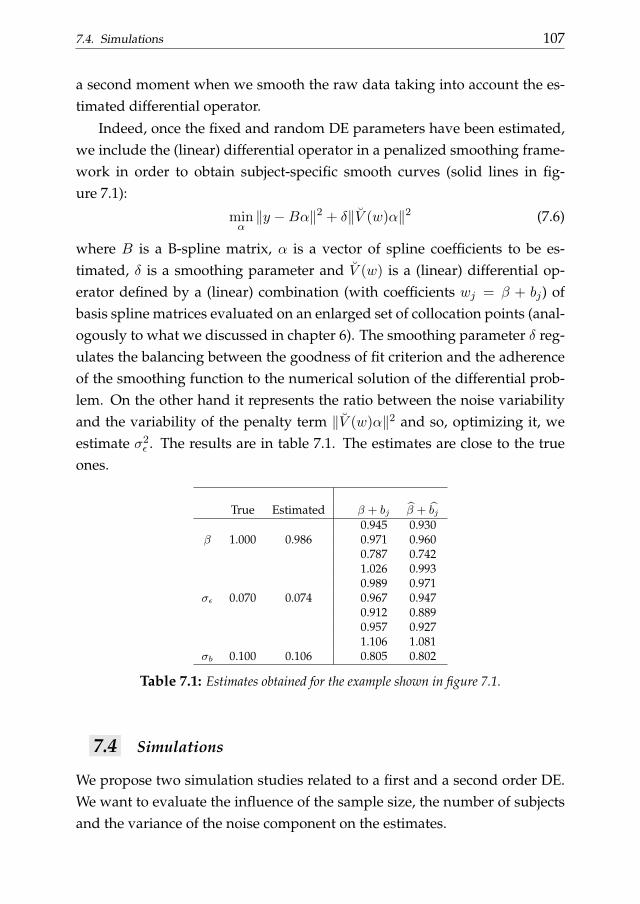
7.4. Simulations 107
a second moment when we smooth the raw data taking into account the es-timated differential operator.
Indeed, once the fixed and random DE parameters have been estimated,we include the (linear) differential operator in a penalized smoothing frame-work in order to obtain subject-specific smooth curves (solid lines in fig-ure 7.1):
minα‖y −Bα‖2 + δ‖V (w)α‖2 (7.6)
where B is a B-spline matrix, α is a vector of spline coefficients to be es-timated, δ is a smoothing parameter and V (w) is a (linear) differential op-erator defined by a (linear) combination (with coefficients wj = β + bj) ofbasis spline matrices evaluated on an enlarged set of collocation points (anal-ogously to what we discussed in chapter 6). The smoothing parameter δ reg-ulates the balancing between the goodness of fit criterion and the adherenceof the smoothing function to the numerical solution of the differential prob-lem. On the other hand it represents the ratio between the noise variabilityand the variability of the penalty term ‖V (w)α‖2 and so, optimizing it, weestimate σ2
ε . The results are in table 7.1. The estimates are close to the trueones.
True Estimated β + bj β + bj0.945 0.930
β 1.000 0.986 0.971 0.9600.787 0.7421.026 0.9930.989 0.971
σε 0.070 0.074 0.967 0.9470.912 0.8890.957 0.9271.106 1.081
σb 0.100 0.106 0.805 0.802
Table 7.1: Estimates obtained for the example shown in figure 7.1.
7.4 Simulations
We propose two simulation studies related to a first and a second order DE.We want to evaluate the influence of the sample size, the number of subjectsand the variance of the noise component on the estimates.
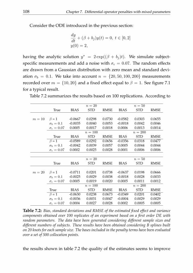
108 Chapter 7. Differential operator penalties with mixed parameters
Consider the ODE introduced in the previous section:
dy
dt+ (β + bj)y(t) = 0, t ∈ [0, 2]
y(0) = 2,
having the analytic solution y∗ = 2 exp((β + bj)t). We simulate subject-specific measurements and add a noise with σε = 0.07. The random effectsare drawn from a Gaussian distribution with zero mean and standard devi-ation σb = 0.1. We take into account n = 20, 50, 100, 200 measurementsrecorded over m = 10, 20 and a fixed effect equal to β = 1. See figure 7.1for a typical result.
Table 7.2 summarizes the results based on 100 replications. According to
n = 20 n = 50True BIAS STD RMSE BIAS STD RMSE
m = 10 β = 1 -0.0667 0.0298 0.0730 -0.0582 0.0303 0.0655σb = 0.1 -0.0035 0.0040 0.0053 -0.0018 0.0042 0.0046σε = 0.07 0.0005 0.0017 0.0018 0.0006 0.0013 0.0014
n = 100 n = 200True BIAS STD RMSE BIAS STD RMSE
β = 1 -0.0589 0.0292 0.0656 -0.0356 0.0318 0.0477σb = 0.1 -0.0042 0.0039 0.0057 0.0005 0.0044 0.0044σε = 0.07 0.0002 0.0025 0.0028 0.0001 0.0006 0.0006
n = 20 n = 50True BIAS STD RMSE BIAS STD RMSE
m = 20 β = 1 -0.0711 0.0201 0.0738 -0.0637 0.0198 0.0666σb = 0.1 -0.0025 0.0029 0.0038 -0.0018 0.0028 0.0033σε = 0.07 0.0005 0.0019 0.0020 0.0005 0.0011 0.0012
n = 100 n = 200True BIAS STD RMSE BIAS STD RMSEβ = 1 -0.0630 0.0238 0.0673 -0.0349 0.0201 0.0402σb = 0.1 -0.0036 0.0031 0.0047 -0.0004 0.0029 0.0029σε = 0.07 0.0004 0.0027 0.0028 0.0002 0.0005 0.0005
Table 7.2: Bias, standard deviations and RMSE of the estimated fixed effect and variancecomponents obtained over 100 replicates of an experiment based on a first order DE withrandom parameters. The data have been generated considering different sample sizes anddifferent numbers of subjects. These results have been obtained considering B splines builton 20 knots for each sample size. The bases included in the penalty terms have been evaluatedover a set of 500 collocation points.
the results shown in table 7.2 the quality of the estimates seems to improve
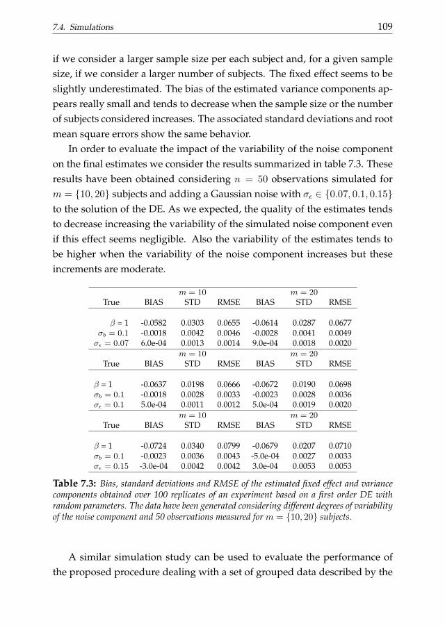
7.4. Simulations 109
if we consider a larger sample size per each subject and, for a given samplesize, if we consider a larger number of subjects. The fixed effect seems to beslightly underestimated. The bias of the estimated variance components ap-pears really small and tends to decrease when the sample size or the numberof subjects considered increases. The associated standard deviations and rootmean square errors show the same behavior.
In order to evaluate the impact of the variability of the noise componenton the final estimates we consider the results summarized in table 7.3. Theseresults have been obtained considering n = 50 observations simulated form = 10, 20 subjects and adding a Gaussian noise with σε ∈ 0.07, 0.1, 0.15to the solution of the DE. As we expected, the quality of the estimates tendsto decrease increasing the variability of the simulated noise component evenif this effect seems negligible. Also the variability of the estimates tends tobe higher when the variability of the noise component increases but theseincrements are moderate.
m = 10 m = 20True BIAS STD RMSE BIAS STD RMSE
β = 1 -0.0582 0.0303 0.0655 -0.0614 0.0287 0.0677σb = 0.1 -0.0018 0.0042 0.0046 -0.0028 0.0041 0.0049σε = 0.07 6.0e-04 0.0013 0.0014 9.0e-04 0.0018 0.0020
m = 10 m = 20True BIAS STD RMSE BIAS STD RMSE
β = 1 -0.0637 0.0198 0.0666 -0.0672 0.0190 0.0698σb = 0.1 -0.0018 0.0028 0.0033 -0.0023 0.0028 0.0036σε = 0.1 5.0e-04 0.0011 0.0012 5.0e-04 0.0019 0.0020
m = 10 m = 20True BIAS STD RMSE BIAS STD RMSE
β = 1 -0.0724 0.0340 0.0799 -0.0679 0.0207 0.0710σb = 0.1 -0.0023 0.0036 0.0043 -5.0e-04 0.0027 0.0033σε = 0.15 -3.0e-04 0.0042 0.0042 3.0e-04 0.0053 0.0053
Table 7.3: Bias, standard deviations and RMSE of the estimated fixed effect and variancecomponents obtained over 100 replicates of an experiment based on a first order DE withrandom parameters. The data have been generated considering different degrees of variabilityof the noise component and 50 observations measured for m = 10, 20 subjects.
A similar simulation study can be used to evaluate the performance ofthe proposed procedure dealing with a set of grouped data described by the
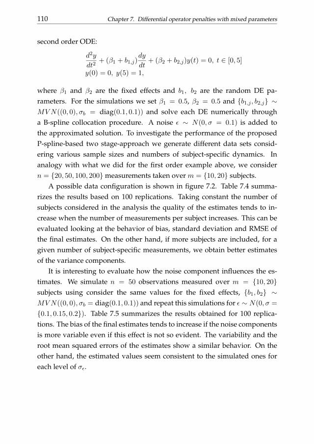
110 Chapter 7. Differential operator penalties with mixed parameters
second order ODE:
d2y
dt2+ (β1 + b1,j)
dy
dt+ (β2 + b2,j)y(t) = 0, t ∈ [0, 5]
y(0) = 0, y(5) = 1,
where β1 and β2 are the fixed effects and b1, b2 are the random DE pa-rameters. For the simulations we set β1 = 0.5, β2 = 0.5 and b1,j , b2,j ∼MVN((0, 0), σb = diag(0.1, 0.1)) and solve each DE numerically througha B-spline collocation procedure. A noise ε ∼ N(0, σ = 0.1) is added tothe approximated solution. To investigate the performance of the proposedP-spline-based two stage-approach we generate different data sets consid-ering various sample sizes and numbers of subject-specific dynamics. Inanalogy with what we did for the first order example above, we considern = 20, 50, 100, 200measurements taken over m = 10, 20 subjects.
A possible data configuration is shown in figure 7.2. Table 7.4 summa-rizes the results based on 100 replications. Taking constant the number ofsubjects considered in the analysis the quality of the estimates tends to in-crease when the number of measurements per subject increases. This can beevaluated looking at the behavior of bias, standard deviation and RMSE ofthe final estimates. On the other hand, if more subjects are included, for agiven number of subject-specific measurements, we obtain better estimatesof the variance components.
It is interesting to evaluate how the noise component influences the es-timates. We simulate n = 50 observations measured over m = 10, 20subjects using consider the same values for the fixed effects, b1, b2 ∼MVN((0, 0), σb = diag(0.1, 0.1)) and repeat this simulations for ε ∼ N(0, σ =
0.1, 0.15, 0.2). Table 7.5 summarizes the results obtained for 100 replica-tions. The bias of the final estimates tends to increase if the noise componentsis more variable even if this effect is not so evident. The variability and theroot mean squared errors of the estimates show a similar behavior. On theother hand, the estimated values seem consistent to the simulated ones foreach level of σε.
7.4. Simulations 111
n = 20 n = 50True BIAS STD RMSE BIAS STD RMSE
m = 10 β1 = 0.5 -0.0185 0.0368 0.0410 -0.0205 0.0325 0.0383β2 = 0.5 -0.0138 0.0341 0.0366 -0.0184 0.0295 0.0347σb1 = 0.1 -0.0016 0.0044 0.0047 -0.0013 0.0049 0.0050σb2 = 0.1 -0.0025 0.0037 0.0044 -0.0011 0.0059 0.0060σε = 0.1 0.0019 0.0045 0.0049 0.0003 0.0022 0.0022
n = 100 n = 200True BIAS STD RMSE BIAS STD RMSE
β1 = 0.5 -0.0237 0.0335 0.0409 -0.0063 0.0341 0.0345β2 = 0.5 -0.0230 0.0319 0.0392 -0.0025 0.0348 0.0347σb1 = 0.1 -0.0011 0.0048 0.0049 -0.0014 0.0043 0.0046σb2 = 0.1 -0.0013 0.0045 0.0047 -0.0012 0.0039 0.0041σε = 0.1 -0.0001 0.0014 0.0014 1.2e-05 0.0011 0.0011
n = 20 n = 50True BIAS STD RMSE BIAS STD RMSE
m = 20 β1 = 0.5 -0.0216 0.0225 0.0311 -0.0235 0.0218 0.0320β2 = 0.5 -0.0063 0.0224 0.0232 -0.0131 0.0244 0.0276σb1 = 0.1 -0.0007 0.0034 0.0035 9.5e-05 0.0035 0.0035σb2 = 0.1 -0.0017 0.0031 0.0035 -0.0014 0.0029 0.0032σε = 0.1 0.0026 0.0081 0.0085 0.00010 0.0022 0.0022
n = 100 n = 200True BIAS STD RMSE BIAS STD RMSE
β1 = 0.5 -0.0214 0.0217 0.0305 -0.0088 0.0199 0.0217β2 = 0.5 -0.0227 0.0202 0.0304 -0.0084 0.0218 0.0232σb1 = 0.1 -0.0009 0.0030 0.0031 -0.0007 0.0036 0.0036σb2 = 0.1 -0.0008 0.0026 0.0028 -5.2e-05 0.0036 0.0036σε = 0.1 -0.0002 0.0015 0.0015 -5.6e-05 0.0009 0.0009
Table 7.4: Bias, standard deviations and RMSE of the estimated fixed effect and variancecomponents obtained over 100 replicates of an experiment based on a second order DE withrandom parameters. The data have been generated considering different sample sizes anddifferent number of subjects.
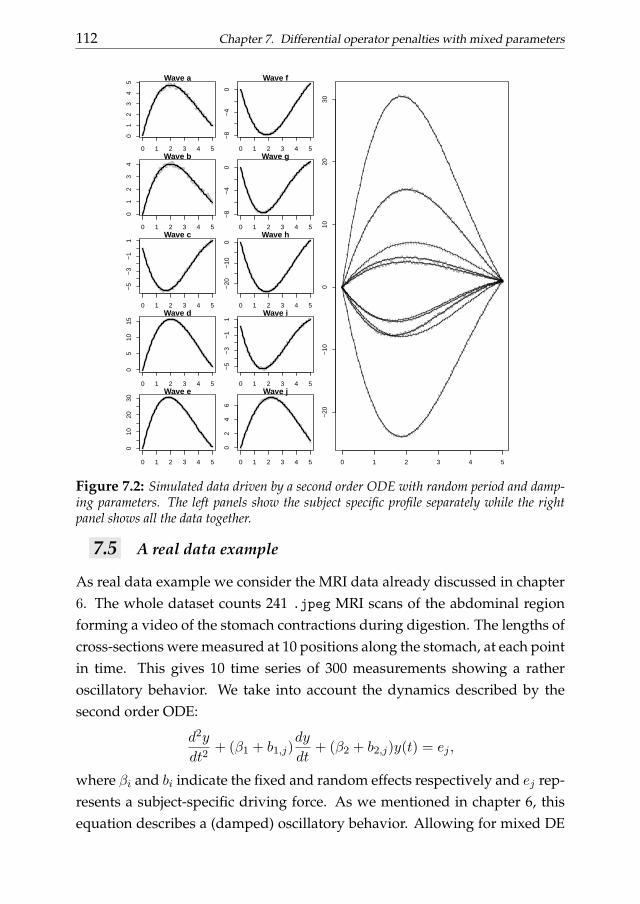
112 Chapter 7. Differential operator penalties with mixed parameters
0 1 2 3 4 5
01
23
45 Wave a
x
0 1 2 3 4 5
01
23
4
Wave b
x
0 1 2 3 4 5
−5
−3
−1
1
Wave c
x
0 1 2 3 4 5
05
1015
Wave d
x
0 1 2 3 4 5
010
2030
Wave e
0 1 2 3 4 5
−8
−4
0
Wave f
x
y
0 1 2 3 4 5−
8−
40
Wave g
x
y
0 1 2 3 4 5
−20
−10
0
Wave h
x
y
0 1 2 3 4 5
−5
−3
−1
1
Wave i
x
y
0 1 2 3 4 5
02
46
Wave j
y
aaaa
aaaaaaaaaaaa
aaaaaaaaaaaaaaaaaaaaaaaaaaaaaaaaaaaaaaaaaaaaaa
aaaaaaaaaaaaaa
aaaaaaaaaaaaaaaaaaaaaaaa
0 1 2 3 4 5
−20
−10
010
2030
dat
bbbbbb
bbbbbbb
bbbbbbbbbbbbbbbbbbbbbbbbbbbbbb
bbbbbbbbbbbbbbbbbbbbbbbbbbbbbbbbbbbbbbbbbbbbbbbbbbbbbbbbb
cccc
cccc
cccc
ccccccccccccccccccccccccccccccccccccccccccccccccccccccccccccccccccccc
ccccccccccccccccccc
d
d
dd
d
dd
ddd
dddddd
dddd
dddd
dddddd
ddddddddddddddddddddd
dddddddddd
dddd
ddddd
ddddd
ddddddd
dddddd
ddddd
ddddddd
e
e
e
e
e
e
e
e
e
e
e
e
e
e
e
e
ee
ee
eeeeeeeeeeeeeee
eeeeeeeeeee
eeeeeee
eeeeeeeee
eee
ee
eeee
eeeeee
eeeeeeeeeeee
eeeee
eeeeee
f ffff f
ff f
ffff f f f
f ff f
ff f f f
f f f f f f f f f f f f f f f f f f f f f f f f f f f f f f f f f f f f f f f f f f f ff f f
f ff f f f
f f f ff f
f f f f ff f
f f f f f f f f f
ggggggg
gggg
ggg
gggggggggg
ggggggggggggggggggggggggggg
gggg
gggg
gggggggggg
ggggggggggggggggggggggggggggg
gg
h
h
h
h
h
h
h
h
h
h
h
h
hh
h
hhh
hhhhhhhhhhhhhhhhhhhhhhhhhhh
hhhhhhhhhhhhhhhhhh
hhh
hhhhhhhhhhhhhhh
hhhh
hhhhhhhhhhhh
hhh
iiiii i
ii i
ii i
i ii i i i i i i i i i i i i i i i i i i i i
i i i i i i i ii i i i i i i i i i i i i i i i i i i i i i i
i i i i i i i i i i i i i i i i i i i i i i i i i i i i i i i i i i
jjjjjj j j
jj j j
j j jj j
j j j j jjj j j
j j j jj j j j j j j j j j j j j j j j j j j j j j j
j j j j j j j j jj j j j j j j j j j j j j j j j j j j j j j j j j
j j j j j j jj j j j j
j
Figure 7.2: Simulated data driven by a second order ODE with random period and damp-ing parameters. The left panels show the subject specific profile separately while the rightpanel shows all the data together.
7.5 A real data example
As real data example we consider the MRI data already discussed in chapter6. The whole dataset counts 241 .jpeg MRI scans of the abdominal regionforming a video of the stomach contractions during digestion. The lengths ofcross-sections were measured at 10 positions along the stomach, at each pointin time. This gives 10 time series of 300 measurements showing a ratheroscillatory behavior. We take into account the dynamics described by thesecond order ODE:
d2y
dt2+ (β1 + b1,j)
dy
dt+ (β2 + b2,j)y(t) = ej ,
where βi and bi indicate the fixed and random effects respectively and ej rep-resents a subject-specific driving force. As we mentioned in chapter 6, thisequation describes a (damped) oscillatory behavior. Allowing for mixed DE
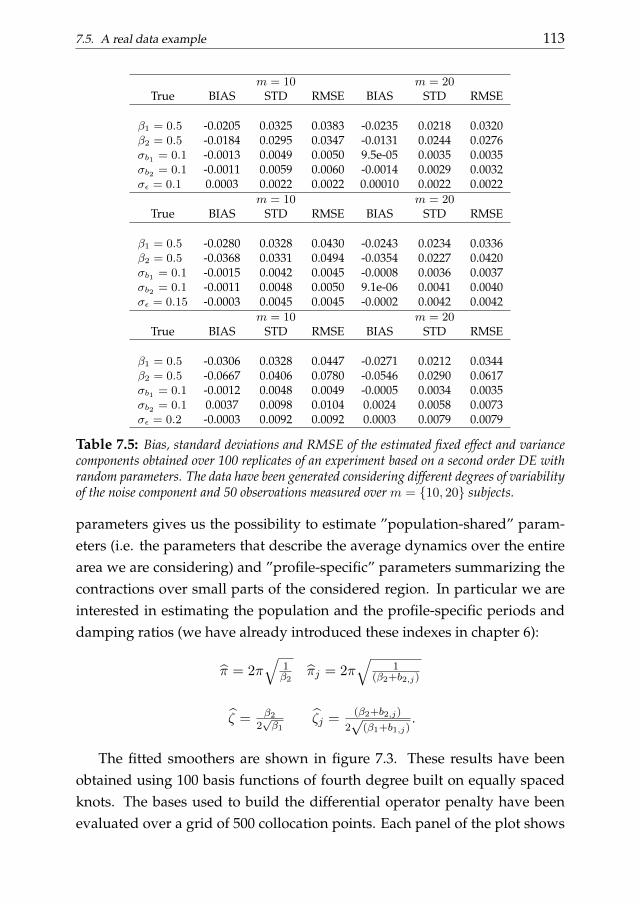
7.5. A real data example 113
m = 10 m = 20True BIAS STD RMSE BIAS STD RMSE
β1 = 0.5 -0.0205 0.0325 0.0383 -0.0235 0.0218 0.0320β2 = 0.5 -0.0184 0.0295 0.0347 -0.0131 0.0244 0.0276σb1 = 0.1 -0.0013 0.0049 0.0050 9.5e-05 0.0035 0.0035σb2 = 0.1 -0.0011 0.0059 0.0060 -0.0014 0.0029 0.0032σε = 0.1 0.0003 0.0022 0.0022 0.00010 0.0022 0.0022
m = 10 m = 20True BIAS STD RMSE BIAS STD RMSE
β1 = 0.5 -0.0280 0.0328 0.0430 -0.0243 0.0234 0.0336β2 = 0.5 -0.0368 0.0331 0.0494 -0.0354 0.0227 0.0420σb1 = 0.1 -0.0015 0.0042 0.0045 -0.0008 0.0036 0.0037σb2 = 0.1 -0.0011 0.0048 0.0050 9.1e-06 0.0041 0.0040σε = 0.15 -0.0003 0.0045 0.0045 -0.0002 0.0042 0.0042
m = 10 m = 20True BIAS STD RMSE BIAS STD RMSE
β1 = 0.5 -0.0306 0.0328 0.0447 -0.0271 0.0212 0.0344β2 = 0.5 -0.0667 0.0406 0.0780 -0.0546 0.0290 0.0617σb1 = 0.1 -0.0012 0.0048 0.0049 -0.0005 0.0034 0.0035σb2 = 0.1 0.0037 0.0098 0.0104 0.0024 0.0058 0.0073σε = 0.2 -0.0003 0.0092 0.0092 0.0003 0.0079 0.0079
Table 7.5: Bias, standard deviations and RMSE of the estimated fixed effect and variancecomponents obtained over 100 replicates of an experiment based on a second order DE withrandom parameters. The data have been generated considering different degrees of variabilityof the noise component and 50 observations measured over m = 10, 20 subjects.
parameters gives us the possibility to estimate ”population-shared” param-eters (i.e. the parameters that describe the average dynamics over the entirearea we are considering) and ”profile-specific” parameters summarizing thecontractions over small parts of the considered region. In particular we areinterested in estimating the population and the profile-specific periods anddamping ratios (we have already introduced these indexes in chapter 6):
π = 2π√
1β2
πj = 2π√
1(β2+b2,j)
ζ = β22√β1
ζj =(β2+b2,j)
2√
(β1+b1,j).
The fitted smoothers are shown in figure 7.3. These results have beenobtained using 100 basis functions of fourth degree built on equally spacedknots. The bases used to build the differential operator penalty have beenevaluated over a grid of 500 collocation points. Each panel of the plot shows
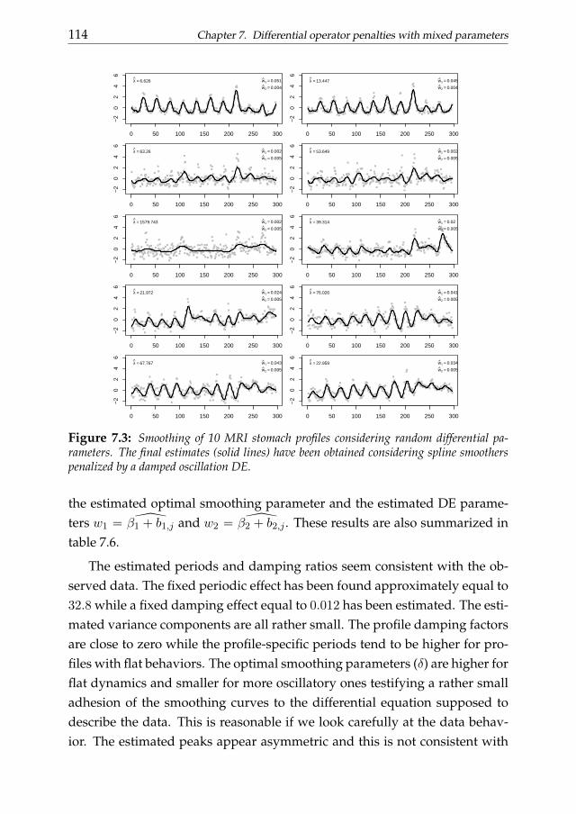
114 Chapter 7. Differential operator penalties with mixed parameters
0 50 100 150 200 250 300
−2
02
46
x
λ = 6.626 w1 = 0.051
w2 = 0.004
0 50 100 150 200 250 300
−2
02
46
x
y
λ = 13.447 w1 = 0.045
w2 = 0.004
0 50 100 150 200 250 300
−2
02
46
x
λ = 63.26 w1 = 0.002
w2 = 0.005
0 50 100 150 200 250 300
−2
02
46
x
y
λ = 53.649 w1 = 0.002
w2 = 0.005
0 50 100 150 200 250 300
−2
02
46
x
λ = 1579.743 w1 = 0.002
w2 = 0.005
0 50 100 150 200 250 300
−2
02
46
x
y
λ = 39.314 w1 = 0.02
w2 = 0.005
0 50 100 150 200 250 300
−2
02
46
x
λ = 21.972 w1 = 0.024
w2 = 0.005
0 50 100 150 200 250 300
−2
02
46
x
y
λ = 76.026 w1 = 0.041
w2 = 0.005
0 50 100 150 200 250 300
−2
02
46
λ = 67.767 w1 = 0.043
w2 = 0.005
0 50 100 150 200 250 300
−2
02
46
y
λ = 22.959 w1 = 0.034
w2 = 0.005
Figure 7.3: Smoothing of 10 MRI stomach profiles considering random differential pa-rameters. The final estimates (solid lines) have been obtained considering spline smootherspenalized by a damped oscillation DE.
the estimated optimal smoothing parameter and the estimated DE parame-ters w1 = β1 + b1,j and w2 = β2 + b2,j . These results are also summarized intable 7.6.
The estimated periods and damping ratios seem consistent with the ob-served data. The fixed periodic effect has been found approximately equal to32.8 while a fixed damping effect equal to 0.012 has been estimated. The esti-mated variance components are all rather small. The profile damping factorsare close to zero while the profile-specific periods tend to be higher for pro-files with flat behaviors. The optimal smoothing parameters (δ) are higher forflat dynamics and smaller for more oscillatory ones testifying a rather smalladhesion of the smoothing curves to the differential equation supposed todescribe the data. This is reasonable if we look carefully at the data behav-ior. The estimated peaks appear asymmetric and this is not consistent with
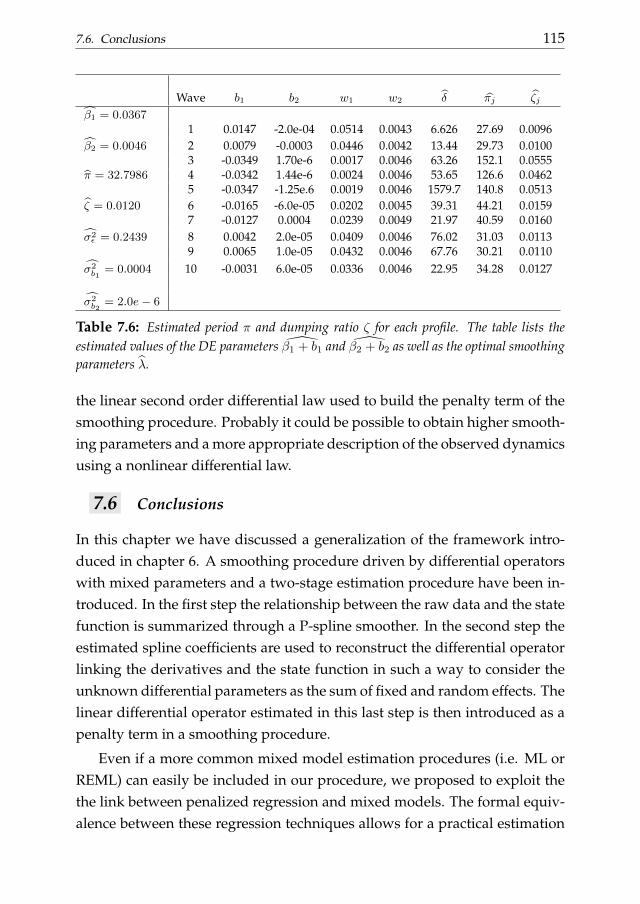
7.6. Conclusions 115
Wave b1 b2 w1 w2 δ πj ζj
β1 = 0.03671 0.0147 -2.0e-04 0.0514 0.0043 6.626 27.69 0.0096
β2 = 0.0046 2 0.0079 -0.0003 0.0446 0.0042 13.44 29.73 0.01003 -0.0349 1.70e-6 0.0017 0.0046 63.26 152.1 0.0555
π = 32.7986 4 -0.0342 1.44e-6 0.0024 0.0046 53.65 126.6 0.04625 -0.0347 -1.25e.6 0.0019 0.0046 1579.7 140.8 0.0513
ζ = 0.0120 6 -0.0165 -6.0e-05 0.0202 0.0045 39.31 44.21 0.01597 -0.0127 0.0004 0.0239 0.0049 21.97 40.59 0.0160
σ2ε = 0.2439 8 0.0042 2.0e-05 0.0409 0.0046 76.02 31.03 0.0113
9 0.0065 1.0e-05 0.0432 0.0046 67.76 30.21 0.0110σ2b1
= 0.0004 10 -0.0031 6.0e-05 0.0336 0.0046 22.95 34.28 0.0127
σ2b2
= 2.0e− 6
Table 7.6: Estimated period π and dumping ratio ζ for each profile. The table lists theestimated values of the DE parameters β1 + b1 and β2 + b2 as well as the optimal smoothingparameters λ.
the linear second order differential law used to build the penalty term of thesmoothing procedure. Probably it could be possible to obtain higher smooth-ing parameters and a more appropriate description of the observed dynamicsusing a nonlinear differential law.
7.6 Conclusions
In this chapter we have discussed a generalization of the framework intro-duced in chapter 6. A smoothing procedure driven by differential operatorswith mixed parameters and a two-stage estimation procedure have been in-troduced. In the first step the relationship between the raw data and the statefunction is summarized through a P-spline smoother. In the second step theestimated spline coefficients are used to reconstruct the differential operatorlinking the derivatives and the state function in such a way to consider theunknown differential parameters as the sum of fixed and random effects. Thelinear differential operator estimated in this last step is then introduced as apenalty term in a smoothing procedure.
Even if a more common mixed model estimation procedures (i.e. ML orREML) can easily be included in our procedure, we proposed to exploit thethe link between penalized regression and mixed models. The formal equiv-alence between these regression techniques allows for a practical estimation
116 Chapter 7. Differential operator penalties with mixed parameters
and interpretation of the variance of the random effects. Indeed we suggest toestimate this variance component optimizing the shrinkage parameter λ bal-ancing between the residual sum of squares criterion and the distributionalhypothesis formulated on the random parameter(s) (induced by a penaltyterm).
The variance of the noise component is estimated using the estimatedsubject-specific differential operators as penalty term in a smoothing proce-dure. This value is obtained optimizing the smoothing parameter (δ) balanc-ing between the fidelity of the final estimates to the data and to a collocationscheme. This smoothing parameter has also another convenient interpreta-tion clarifying the appropriateness of the hypothesized ODE in describingthe data dynamics.
The performance of the proposed procedure has been evaluated consid-ering both simulated and real data. A simulation studies based on first andsecond order differential problems have been discussed. Through simula-tions we have evaluated the influence of the data characteristics on the es-timates obtained using the two stage procedure. We have found that, in-creasing the number of measurements available for each subject and/or thenumber of considered subjects, the bias, the standard deviation and the rootmean squared errors of the estimated fixed effects and variance componentstend to decrease. On the other we found that, even if a moderate number ofobservations and subjects is available, the quality of the estimates obtainedusing the proposed procedure is quite high.
We also discussed a real data example, stomach contractions during di-gestion. In this case we used a linear second order differential equation withmixed parameters to investigate the global and profile-specific contractioncharacteristics. The estimated DE parameters have been found consistentwith the observed data behavior. On the other hand rather small optimalsmoothing parameters have been found using an EM-type procedure. Thisis probably due to the fact that the considered linear DE is not appropriate todescribe the asymmetric oscillations characterizing the observed data behav-ior.
One of the major limitation of our discussion lies in the fact that only lin-ear differential problems have been considered. From a theoretical point ofview the two stage procedure for the estimation of the unknown DE param-

7.6. Conclusions 117
eters can be easily adapted in order to deal with nonlinear mixed effect mod-els. The definition of a nonlinear differential operator penalty can be obtainedadopting some linearization strategy of the differential problem. Smoothingprocedures penalized by nonlinear differential operators will represent oneof the major topic of our future research.

DIFFERENTIAL PENALIZED SMOOTHING IN
TWO DIMENSIONS 8Partial differential equations (PDEs) are common tools to describe dy-
namic systems evolving in more than one dimension. In real data applica-tions the parameters of suitable differential models are usually unknownand need to be estimated from the available measurements of a given phe-nomenon. In this chapter we propose a two-dimensional smoothing ap-proach including a partial differential penalty for the analysis of two-dimensional data approximatively described by PDEs. We also proposea P-spline-based two-stage procedure for the estimation of the unknownDE parameters.Keywords: Partial differential equations, tensor product B-spline collo-cation, tensor product P-splines, penalized smoothing.
8.1 Introduction
Partial differential equations (PDEs) are commonly used to describe dynamicsystems evolving in more than one dimension. In many circumstances, it isdifficult to have a precise knowledge of the differential law governing an ob-served dynamics. Fortunately many two-dimensional phenomena that aredescribed, at least approximately, by partial differential equations can bemeasured. For this reason it is convenient to combine the observed infor-mation with the theoretical behavior of the phenomenon.
In this chapter we propose a differential operator smoothing procedurefor the analysis of data which dynamic is well described by a partial differen-tial equations. We follow the framework defined by Ramsay and Silverman(2005) based on the definition of a penalized smoothing procedure involvingB-spline functions. We suggest to include a penalty term in the smoothingframework approximated by a tensor product B-spline collocation scheme.
119
120 Chapter 8. Differential penalized smoothing in two dimensions
As we already discussed for ODEs, it is not realistic to hypothesize a per-fect knowledge of the differential law governing the observed dynamic andit becomes necessary to reconstruct this mathematical model using the avail-able observations. We propose to estimate the unknown parameters definingthe differential penalty term, using a two-stage approach based on tensorproduct P-splines. In a first step the two-dimensional data trend is sepa-rated from the noise of the observed measurements through a suitable non-isotropic smoother. Then the optimal spline coefficients estimated in the firststep are used to approximate the functions defining the PDE and to estimatethe best differential parameters through least squares. Once the differentialoperator has been reconstructed it is used as penalty in the smoothing proce-dure. The balance between the fidelity to the data and to the approximatedsolution of the PDE is tuned by a smoothing parameter.
This chapter is organized as follows: section 8.2 introduces the PDE-basedpenalized smoothing approach considering known differential operators, insection 8.3 we abandon the unrealistic hypothesis of knowledge of the differ-ential law and introduce a two-stage procedure for the estimation of the un-known DE parameters while in section 8.4 the performance of the proposedprocedure is evaluated through simulations.
8.2 PDE-based penalized smoothing
Suppose we observe a set of data (z) which dynamics is well described by apartial differential equation. What happens if our knowledge about the dif-ferential equation describing the observed dynamic is not precise or even notcorrect? In this case the solution of the differential problem would provide aninadequate description of the observed measurements. Unfortunately, this isnot a remote eventuality given that small changes of the parameters or ofthe conditions defining the differential problem can lead to really differentnumerical solutions
It is possible to overcome this problem forcing the solution of the DEwe have in mind to give an appropriate description of the data. Thiscan be achieved using a smoothing approach penalized by a differentialoperator consistent with a collocation scheme. If we define as u(x, y) =∑n
i
∑mj (Byj ⊗ Bxi)cij the approximated two-dimensional state function
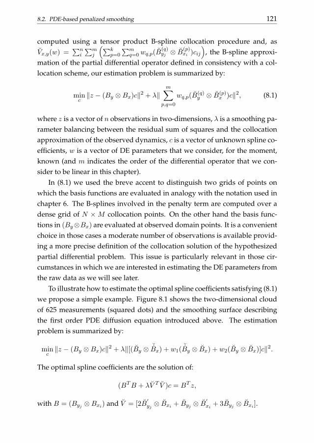
8.2. PDE-based penalized smoothing 121
computed using a tensor product B-spline collocation procedure and, asVx,y(w) =
∑ni
∑mj
(∑kp=0
∑mq=0wq,p(B
(q)yj ⊗ B
(p)xi )cij
), the B-spline approxi-
mation of the partial differential operator defined in consistency with a col-location scheme, our estimation problem is summarized by:
minc‖z − (By ⊗Bx)c‖2 + λ‖
m∑p,q=0
wq,p(B(q)y ⊗ B(p)
x )c‖2, (8.1)
where z is a vector of n observations in two-dimensions, λ is a smoothing pa-rameter balancing between the residual sum of squares and the collocationapproximation of the observed dynamics, c is a vector of unknown spline co-efficients, w is a vector of DE parameters that we consider, for the moment,known (and m indicates the order of the differential operator that we con-sider to be linear in this chapter).
In (8.1) we used the breve accent to distinguish two grids of points onwhich the basis functions are evaluated in analogy with the notation used inchapter 6. The B-splines involved in the penalty term are computed over adense grid of N ×M collocation points. On the other hand the basis func-tions in (By⊗Bx) are evaluated at observed domain points. It is a convenientchoice in those cases a moderate number of observations is available provid-ing a more precise definition of the collocation solution of the hypothesizedpartial differential problem. This issue is particularly relevant in those cir-cumstances in which we are interested in estimating the DE parameters fromthe raw data as we will see later.
To illustrate how to estimate the optimal spline coefficients satisfying (8.1)we propose a simple example. Figure 8.1 shows the two-dimensional cloudof 625 measurements (squared dots) and the smoothing surface describingthe first order PDE diffusion equation introduced above. The estimationproblem is summarized by:
minc‖z − (By ⊗Bx)c‖2 + λ‖[(By ⊗ ˘Bx) + w1( ˘By ⊗ Bx) + w2(By ⊗ Bx)]c‖2.
The optimal spline coefficients are the solution of:
(BTB + λV T V )c = BT z,
with B = (Byj ⊗Bxi) and V = [2B′yj ⊗ Bxi + Byj ⊗ B
′xi + 3Byj ⊗ Bxi ].
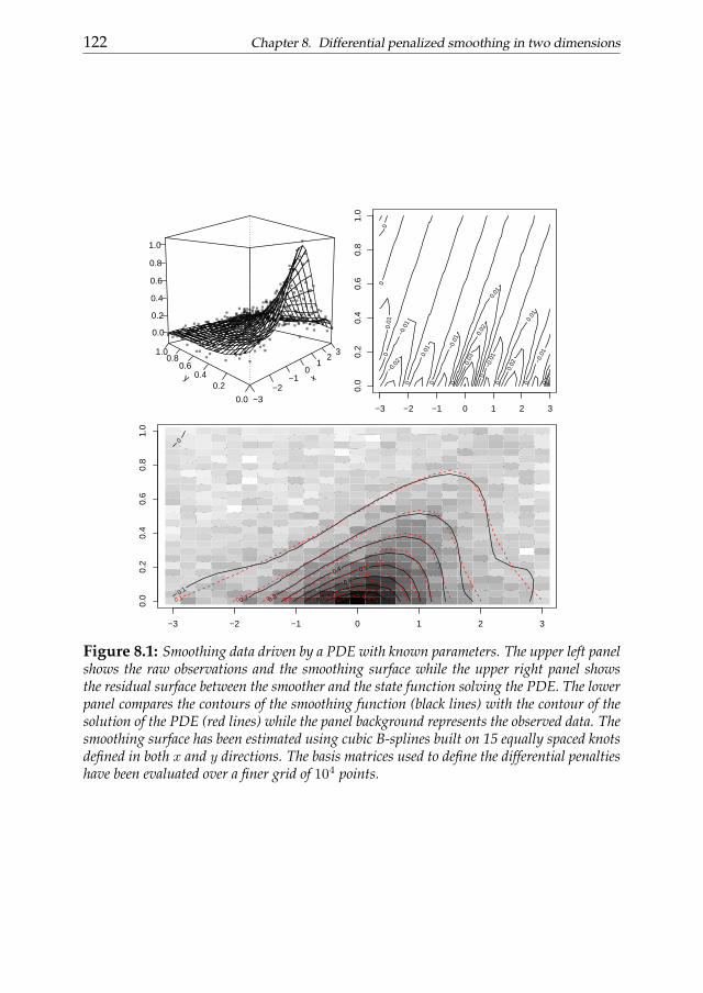
122 Chapter 8. Differential penalized smoothing in two dimensions
x
−3−2
−10
12
3
y
0.0
0.20.4
0.60.8
1.0
0.0
0.2
0.4
0.6
0.8
1.0
−0.
02
−0.
01
−0.
01
−0.
01
−0.
01
0
0
0
0
0
0 0
0
0
0
0.0
1
0.0
1
0.0
1
0.0
1
0.0
2
0.0
2 0.0
3
−3 −2 −1 0 1 2 3
0.0
0.2
0.4
0.6
0.8
1.0
−0.05
−0.05
0
0
0
0
0
0
0
0
0
0
0
0
0
0
0
0
0.05
0.05
0.0
5
0.05
0.05
0.05
0.05
0.05
0.05
0.05
0.05
0.1
0.1
0.1 0.1
0.1
0.15
0.15
0.15
0.2
0.2
0.2 0.25
0.3
0.35 0.4 0.45
0.5
0.55
0.6
0.65
0.75
−3 −2 −1 0 1 2 3
0.0
0.2
0.4
0.6
0.8
1.0
0
0.1
0.2 0.3
0.4 0.5
0.6
0.7 0.8
0.1 0.2
0.3 0.4
0.5
0.6 0.7
0.8 0.9
Figure 8.1: Smoothing data driven by a PDE with known parameters. The upper left panelshows the raw observations and the smoothing surface while the upper right panel showsthe residual surface between the smoother and the state function solving the PDE. The lowerpanel compares the contours of the smoothing function (black lines) with the contour of thesolution of the PDE (red lines) while the panel background represents the observed data. Thesmoothing surface has been estimated using cubic B-splines built on 15 equally spaced knotsdefined in both x and y directions. The basis matrices used to define the differential penaltieshave been evaluated over a finer grid of 104 points.
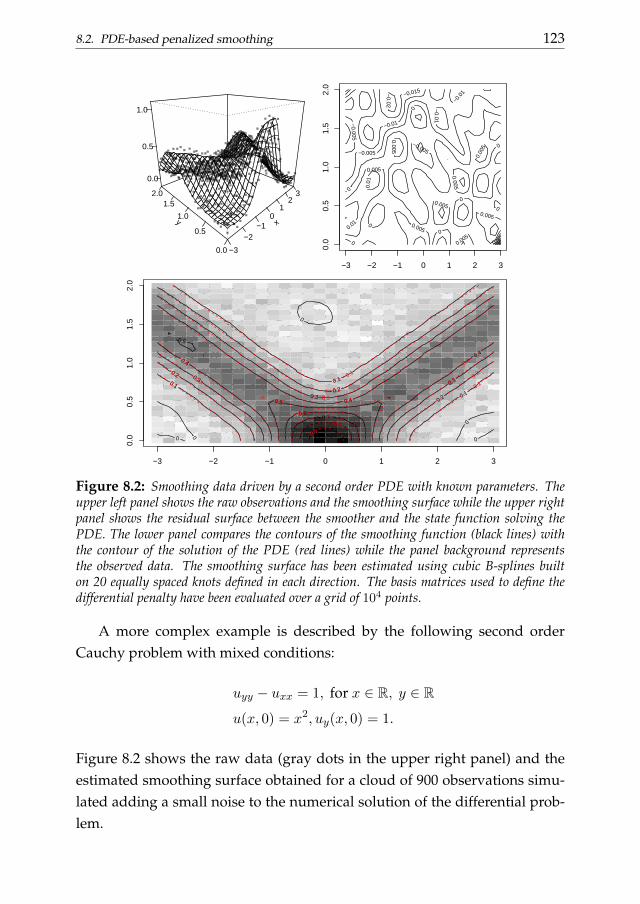
8.2. PDE-based penalized smoothing 123
x
−3
−2−1
01
23
y
0.0
0.5
1.0
1.52.0
0.0
0.5
1.0
−0.02
−0.015
−0.01
−0.01
−0.
01
−0.005
−0.005
−0.005
0
0
0
0
0
0
0
0
0
0.005
0.005
0.005
0.005
0.005
0.005
0.005
0.0
05
0.01
0.0
1
−3 −2 −1 0 1 2 3
0.0
0.5
1.0
1.5
2.0
−0.05
−0.05
0
0
0
0
0
0
0
0
0
0
0
0
0
0
0 0
0
0
0
0
0
0
0
0.05
0.05
0.05
0.05
0.05
0.05 0.1
0.1
0.1
0.15
0.15
0.15
0.2
0.2
0.2 0.25
0.25 0.25
0.3
0.3
0.3
0.35
0.35
0.35
0.4
0.4
0.4
0.45
0.45
0.45
0.45
0.5
0.5
0.5
0.5
0.5
0.5
0.5
0.5
0.55
0.55
0.6 0.65 0.7 0.75
0.8
0.85 0.9
−3 −2 −1 0 1 2 3
0.0
0.5
1.0
1.5
2.0
0
0
0
0
0
0.1 0.1
0.1
0.2
0.2
0.2
0.3
0.3
0.3
0.4
0.4
0.4
0.5
0.5
0.6 0.7
0.8
0.9
0.1
0.1
0.1
0.2
0.2
0.2 0.3
0.3
0.3
0.4
0.4
0.4
0.5
0.6 0.7
0.8
0.9
Figure 8.2: Smoothing data driven by a second order PDE with known parameters. Theupper left panel shows the raw observations and the smoothing surface while the upper rightpanel shows the residual surface between the smoother and the state function solving thePDE. The lower panel compares the contours of the smoothing function (black lines) withthe contour of the solution of the PDE (red lines) while the panel background representsthe observed data. The smoothing surface has been estimated using cubic B-splines builton 20 equally spaced knots defined in each direction. The basis matrices used to define thedifferential penalty have been evaluated over a grid of 104 points.
A more complex example is described by the following second orderCauchy problem with mixed conditions:
uyy − uxx = 1, for x ∈ R, y ∈ R
u(x, 0) = x2, uy(x, 0) = 1.
Figure 8.2 shows the raw data (gray dots in the upper right panel) and theestimated smoothing surface obtained for a cloud of 900 observations simu-lated adding a small noise to the numerical solution of the differential prob-lem.
124 Chapter 8. Differential penalized smoothing in two dimensions
8.3 Two-dimensional smoothing with unknown partialdifferential penalties
In many applications we have only a vague idea about the differentiallaw that could approximate a set of measurements describing a given phe-nomenon. A possibility consists in reconstructing the mathematical law wehave in mind using the available observations.
This problem leads to the estimation of the unknown parameters definingthe PDE. A possible approach consists in writing the analytic or numericalsolution of the equation as explicit function of the unknown parameters esti-mated from the data. This generally leads to a nonlinear regression problemeven if the PDE is linear. An alternative approach is to incorporate the partialdifferential equation as a penalty in a smoothing framework as suggested byRamsay (2002) and Wood et al. (2008). This second approach is the one wefollow here suggesting a tensor product P-spline-based two-stage procedurefor the estimation of the unknown DE parameters.
We want to approximate the observed measurements in such a way thefinal estimates are consistent with the solution of the PDE. To reach this goalwe need to estimate its unknown parameters. Our estimation problem canbe summarized as follows:
minw,c‖z − (By ⊗Bx)c‖2 + λ‖V c‖2, (8.2)
where By ⊗ Bx = B is a tensor product basis matrix, c is a vector of splinecoefficients, λ is a smoothing parameter controlling the amount of penaltyapplied to the least squares criterion, V is the B-spline approximation of a(linear) partial differential operator defined using a collocation scheme. Thisoperator depends on the vector of weights w.
The unknown DE parameters can be estimated through a two-stage pro-cedure. In analogy with what we discussed in chapter 6, we move from theconsideration that the approximated state function implied in the PDE in thepenalty term has to be consistent with the signal behind the observationsif the differential model we have in mind is appropriate. This signal canbe extracted from the noisy measurements using a tensor product P-spline.This smoother has to be able to separate the signal from the noise compo-nent of the raw observations. A possibility is to select the couple of optimal
8.3. Two-dimensional smoothing with unknown partial differential penalties 125
smoothing parameter through an automatic procedure. The optimal splinecoefficients defining the two-dimensional smoother provide a compact rep-resentation of the state function. Multiplying these coefficients by the basismatrices defining V we obtain an approximation of the functions involvedin the differential law. Once these functions have been approximated the pa-rameter vector w can be estimated using least squares.
The smoothing parameter in (8.2) plays a crucial role. It regulates the rel-ative importance of the residual sum of squares criterion over the collocationsolution of the differential equation in determining the shape of the final fit.For λ→ 0 the smoothing surface tends to be rough given that the estimationprocedure is driven exclusively by a residual sum of squares. On the otherhand, for λ→∞ the estimated surface tends to mimic the numerical solutionof the differential equation included in the penalty term.
Given the estimated differential parameters, it is possible to define thepenalty term V and estimate the optimal spline coefficients:
c = (BTB + λV T V )−1BT z (8.3)
The optimal smoothing parameter λ can be selected using an automatic pro-cedure. In the examples shown in this chapter we use an EM-type approach.
Figure 8.3 shows an example of the results obtained using the describedapproach. The top panels show the estimated smoother and the residualsbetween the fitting surface and the analytic solution of the differential prob-lem while the lower panel shows a contour representation of the data and thesmoothing function. The data have been generated taking into account thefollowing PDE:
uyy − 4uxx = 0, ∀x ∈ R, y ∈ R+
u(x, 0) = exp(−x2), uy(x, 0) = 0.
The observations (squared dots in the left upper panel of figure 8.3) havebeen simulated adding a Gaussian noise to the approximated solution of thisdifferential problem computed over xi ∈ [−3, 3], yj ∈ [0, 2]. The DE parame-ter has been estimated equal to w = −4.067.
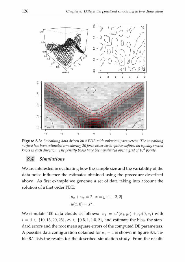
126 Chapter 8. Differential penalized smoothing in two dimensions
x
−3
−2−1
01
23
y
0.0
0.5
1.0
1.52.0
0.0
0.5
1.0
−0.
01
−0.
01
−0.01
−0.01
−0.01
−0.01
0
0
0
0
0
0
0
0
0
0
0.0
1
0.01
0.01
0.0
1
−3 −2 −1 0 1 2 3
0.0
0.5
1.0
1.5
2.0
−0.05
−0.05
0
0
0
0
0
0
0
0
0
0
0
0
0
0
0 0
0
0
0
0
0
0
0
0.05
0.05
0.05
0.05
0.05
0.05 0.1
0.1
0.1
0.15
0.15
0.15
0.2
0.2
0.2 0.25
0.25 0.25
0.3
0.3
0.3
0.35
0.35
0.35
0.4
0.4
0.4
0.45
0.45
0.45
0.45
0.5
0.5
0.5
0.5
0.5
0.5
0.5
0.5
0.55
0.55
0.6 0.65 0.7 0.75
0.8
0.85 0.9
−3 −2 −1 0 1 2 3
0.0
0.5
1.0
1.5
2.0
0
0
0
0
0
0.1 0.1
0.1
0.2
0.2
0.2
0.3
0.3
0.3
0.4
0.4
0.4
0.5
0.5
0.6 0.7
0.8
0.9
0.1
0.1
0.1
0.2
0.2
0.2 0.3
0.3
0.3
0.4
0.4
0.4
0.5
0.6 0.7
0.8
0.9
Figure 8.3: Smoothing data driven by a PDE with unknown parameters. The smoothingsurface has been estimated considering 20 forth order basis splines defined on equally spacedknots in each direction. The penalty bases have been evaluated over a grid of 104 points.
8.4 Simulations
We are interested in evaluating how the sample size and the variability of thedata noise influence the estimates obtained using the procedure describedabove. As first example we generate a set of data taking into account thesolution of a first order PDE:
ux + uy = 2, x = y ∈ [−2, 2]
u(x, 0) = x2.
We simulate 100 data clouds as follows: zij = u∗(xj , yj) + εij(0, σε) withi = j ∈ 10, 15, 20, 25, σε ∈ 0.5, 1, 1.5, 2, and estimate the bias, the stan-dard errors and the root mean square errors of the computed DE parameters.A possible data configuration obtained for σε = 1 is shown in figure 8.4. Ta-ble 8.1 lists the results for the described simulation study. From the results

8.4. Simulations 127
N=100
−2 −1 0 1 2
−2
−1
01
2
N=225
−2 −1 0 1 2
−2
−1
01
2
N=400
−2 −1 0 1 2
−2
−1
01
2
N=625
−2 −1 0 1 2
−2
−1
01
2
Figure 8.4: Smoothing data driven by a first order PDE with unknown parameters. Eachpanel describes the smoothing surface obtained for different sample sizes. The estimates havebeen performed considering cubic B-splines built on 10 equally spaced knots selected on bothx and y directions.
it is possible to notice that the quality of the estimates tends to be lower iflower sample sizes are considered. Indeed, for larger sample sizes the bias,the standard deviation and the root mean square errors tend to be smallertaking constant the variability of the noise component. On the other hand,for a given sample size, the quality of the estimates tends to decrease if weconsider a higher noise variability.
A similar simulation study can be conducted taking into account a morecomplex PDE:
uyy − uxx = 1, x = y ∈ [−2, 2]
u(x, 0) = x2, uy(x, 0) = 1.
We simulate 100 series of data: zij = u∗(xj , yj) + εij(0, σε) with i = j ∈10, 15, 20, 25, σε ∈ 0.5, 1, 1.5, 2, and estimate the bias, the standard errors

128 Chapter 8. Differential penalized smoothing in two dimensions
i = j = 10 i = j = 15True w = 1 BIAS STD RMSE BIAS STD RMSE
σε = 0.5 0.0019 0.0232 0.0232 -0.0023 0.0170 0.0171
σε = 1 -0.0114 0.0568 0.0577 -0.0125 0.0394 0.0412
σε = 1.5 -0.0255 0.0669 0.0712 -0.0055 0.0475 0.0476
σε = 2 -0.0455 0.1039 0.1130 -0.0090 0.0755 0.0757
i = j = 20 i = j = 25True w = 1 BIAS STD RMSE BIAS STD RMSE
σε = 0.5 -2.0e-04 0.0138 0.0137 0.0018 0.0122 0.0123
σε = 1 0.0031 0.0307 0.0307 0.0040 0.0274 0.0276
σε = 1.5 -0.0073 0.0439 0.0443 -9.0e-04 0.0383 0.0381
σε = 2 -0.0172 0.0549 0.0573 0.0025 0.0545 0.0543
Table 8.1: Bias, standard deviation and RMSE of the DE parameter estimated for a firstorder partial differential problem.
and the root mean square errors of the computed DE parameters. A possibledata configuration obtained considering σε = 1 is shown in figure 8.5. Ta-ble 8.2 summarizes the results obtained for the described experiment. Againthe quality of the estimates seems to be higher for larger sample sizes andto decrease if we consider more variable noise components for each samplesize.
8.5 Conclusions
In this chapter we have introduced a PDE-based penalized smoothing ap-proach for the analysis of two-dimensional data which dynamics is approxi-mately described by a partial differential law. Our approach involves a com-bination of tensor product basis spline functions for the approximation ofthe differential penalty in analogy with a tensor product B-spline collocationscheme.
In presence of unknown PDE parameters we adopt a two stage estima-tion procedure: 1) smooth the raw data using a P-spline smoother able toremove the noise, 2) estimate the DE parameters through least squares. Thissimplification separates the computation of the DE parameters from the data
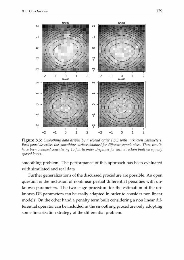
8.5. Conclusions 129
N=100
−2 −1 0 1 2
−2
−1
01
2
N=225
−2 −1 0 1 2
−2
−1
01
2
N=400
−2 −1 0 1 2
−2
−1
01
2
N=625
−2 −1 0 1 2
−2
−1
01
2
Figure 8.5: Smoothing data driven by a second order PDE with unknown parameters.Each panel describes the smoothing surface obtained for different sample sizes. These resultshave been obtained considering 15 fourth order B-splines for each direction built on equallyspaced knots.
smoothing problem. The performance of this approach has been evaluatedwith simulated and real data.
Further generalizations of the discussed procedure are possible. An openquestion is the inclusion of nonlinear partial differential penalties with un-known parameters. The two stage procedure for the estimation of the un-known DE parameters can be easily adapted in order to consider non linearmodels. On the other hand a penalty term built considering a non linear dif-ferential operator can be included in the smoothing procedure only adoptingsome linearization strategy of the differential problem.

130 Chapter 8. Differential penalized smoothing in two dimensions
i = j = 10 i = j = 15True w = −1 BIAS STD RMSE BIAS STD RMSE
σε = 0.5 0.0863 0.0252 0.0899 0.067 0.021 0.0702
σε = 1 0.0894 0.0506 0.1026 0.0599 0.0451 0.0748
σε = 1.5 0.0680 0.0685 0.0963 0.0572 0.0668 0.0877
σε = 2 0.0576 0.1143 0.1275 0.0491 0.0873 0.0998
i = j = 20 i = j = 25True w = −1 BIAS STD RMSE BIAS STD RMSE
σε = 0.5 0.0529 0.0182 0.0559 0.0433 0.015 0.0458
σε = 1 0.0489 0.0361 0.0607 0.0401 0.031 0.0505
σε = 1.5 0.0412 0.0518 0.0660 0.0399 0.0407 0.0569
σε = 2 0.0480 0.0741 0.0880 0.0440 0.0632 0.0767
Table 8.2: Bias, standard deviation and RMSE of the DE parameter estimated for a secondorder partial differential problem.
GENERALIZATIONS OF COLLOCATION BASED
PROCEDURES 9In this chapter we briefly discuss some generalizations of the frame-
work introduced in the previous chapters. The following sections presenta sort of overview of the state of our art in analyzing more complex dy-namics. In particular, we extend the collocation scheme for the solution ofdifferential problems involving some kind of nonlinearity. We deal withdifferential problems involving inequality conditions, delay differentialequations (DDEs) and nonlinear DEs. We also introduce a DDE-basedpenalized smoothing procedure.Keywords: Inequality conditions, asymmetric least squares, delay differ-ential equations, nonlinear ODE, DDE-based penalized smoothing.
9.1 Introduction
The B-spline collocation approach is flexible enough to allow for the solutionof several classes of differential problems. In the previous chapters we fo-cused on linear ordinary and differential equations. Here we concentrate onmore complicated problems: ODE with inequality constraints, delay differ-ential equations (DDE) and nonlinear ODEs.
Inequality constraints can be included in the collocation scheme withasymmetrically weighted penalties. In particular, in this chapter, we dealwith constraints limiting the codomain of the state function and with mono-tonicity constraints.
Delay differential equations or difference differential equations (DDEs)have been introduced in the previous century in the field of automatic con-trol. Any system with a feedback control involves time delays. A time delayarises because a finite time is required to sense information and then to reactto it. In this chapter we evaluate the appropriateness of the B-spline colloca-
131
132 Chapter 9. Generalizations of collocation based procedures
tion scheme for solving this kind of differential equations. We also introducea DDE-based smoothing procedure to analyze data described by delayed dy-namics.
Furthermore, the B-spline collocation scheme can also be applied to non-linear differential equations. In particular we focus on ordinary differentialequations. In order to solve a nonlinear problem through collocation someiterative linearization of the differential operator is needed. In this chapter,we suggest to use a Newton-type linearization method.
This chapter is organized as follows: in section 9.2 we introduce a B-splinecollocation scheme for the solution of ordinary and partial DEs with uncon-ventional conditions through weighted least squares. In section 9.5 the the-oretical aspects about are briefly introduced and a simple problem is solved.In section 9.4 we deal with nonlinear ODEs. In section 9.5 we introduce aDDE-based penalized smoothing procedure for the analysis of data drivenby delay dynamics.
9.2 B-spline collocation solution of differential equations withunconventional conditions
Suppose we are interested in obtaining a numerical solution for a given dif-ferential equation with a set of inequality constraints. An example is thesecond order harmonic oscillation problem described by:
y′′
+ 9y = 0, t ∈ [0, 5]
y(1) = 0, y(5) = 1,
y(t) ≥ −1.
This problem does not have an analytic solution and the inequality constraintmakes it nonlinear. A possible strategy is to face the problem without the lastconstraint and impose that the inequality holds in a least square sense. Inother words it is possible to impose this constraint to the state function usingasymmetrically penalized least squares. The penalty controls for violations
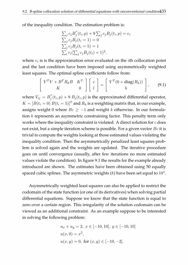
9.2. B-spline collocation solution of differential equations with unconventional conditions133
of the inequality condition. The estimation problem is:∑j cjB
′′j (ti, p) + 9
∑j cjBj(ti, p) = ei∑
j cjBj(ti = 1) = 0∑j cjBj(ti = 5) = 1∑i ri(
∑j cjBj(ti) + 1)2.
where ei is is the approximation error evaluated on the ith collocation pointand the last condition have been imposed using asymmetrically weightedleast squares. The optimal spline coefficients follow from:[
V TV +BTRkB KT
K 0
][c
l
]=
[V T (0 + diag(Rk))
b
], (9.1)
where Vij = B′′j (ti, p) + 9 Bj(ti, p) is the approximated differential operator,
K = [B(ti = 0)B(ti = 5)]T andRk is a weighting matrix that, in our example,assigns weight 0 where Bc ≥ −1 and weight k otherwise. In our formula-tion k represents an asymmetric constraining factor. This penalty term onlyworks where the inequality constraint is violated. A direct solution for c doesnot exist, but a simple iteration scheme is possible. For a given vector Bc it istrivial to compute the weights looking at those estimated values violating theinequality condition. Then the asymmetrically penalized least squares prob-lem is solved again and the weights are updated. The iterative proceduregoes on until convergence (usually, after few iterations no more estimatedvalues violate the condition). In figure 9.1 the results for the example alreadyintroduced are shown. The estimates have been obtained using 50 equallyspaced cubic splines. The asymmetric weights (k) have been set equal to 104.
Asymmetrically weighted least squares can also be applied to restrict thecodomain of the state function (or one of its derivatives) when solving partialdifferential equations. Suppose we know that the state function is equal tozero over a certain region. This irregularity of the solution codomain can beviewed as an additional constraint. As an example suppose to be interestedin solving the following problem:
ux + uy = 2, x ∈ [−10, 10], y ∈ [−10, 10]
u(x, 0) = x2,
u(x, y) = 0, for (x, y) ∈ [−10,−2].
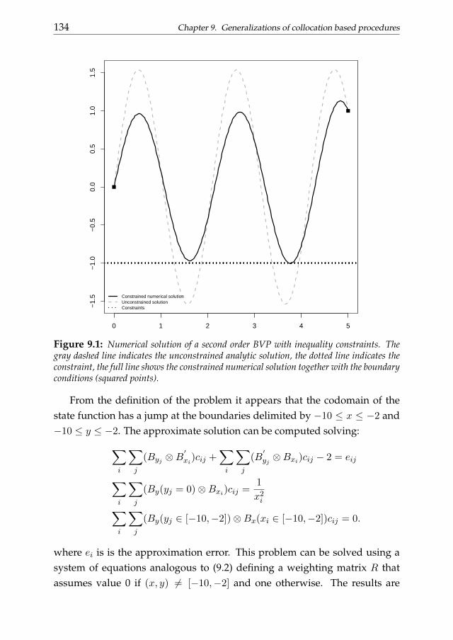
134 Chapter 9. Generalizations of collocation based procedures
0 1 2 3 4 5
−1.
5−
1.0
−0.
50.
00.
51.
01.
5
Constrained numerical solutionUnconstrained solutionConstraints
Figure 9.1: Numerical solution of a second order BVP with inequality constraints. Thegray dashed line indicates the unconstrained analytic solution, the dotted line indicates theconstraint, the full line shows the constrained numerical solution together with the boundaryconditions (squared points).
From the definition of the problem it appears that the codomain of thestate function has a jump at the boundaries delimited by −10 ≤ x ≤ −2 and−10 ≤ y ≤ −2. The approximate solution can be computed solving:∑
i
∑j
(Byj ⊗B′xi)cij +
∑i
∑j
(B′yj ⊗Bxi)cij − 2 = eij
∑i
∑j
(By(yj = 0)⊗Bxi)cij =1
x2i∑
i
∑j
(By(yj ∈ [−10,−2])⊗Bx(xi ∈ [−10,−2])cij = 0.
where ei is is the approximation error. This problem can be solved using asystem of equations analogous to (9.2) defining a weighting matrix R thatassumes value 0 if (x, y) 6= [−10,−2] and one otherwise. The results are
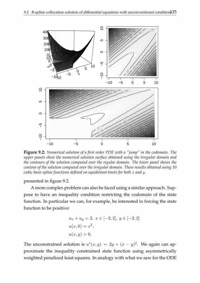
9.2. B-spline collocation solution of differential equations with unconventional conditions135
x−10
−50
510y
−10
−50
510
0100
200
300
400
−10 −5 0 5 10
−10
−5
05
10
−10 −5 0 5 10
−10
−5
05
10
Figure 9.2: Numerical solution of a first order PDE with a ”jump” in the codomain. Theupper panels show the numerical solution surface obtained using the irregular domain andthe contours of the solution computed over the regular domain. The lower panel shows thecontour of the solution computed over the irregular domain. These results obtained using 10cubic basis spline functions defined on equidistant knots for both x and y.
presented in figure 9.2.A more complex problem can also be faced using a similar approach. Sup-
pose to have an inequality condition restricting the codomain of the statefunction. In particular we can, for example, be interested in forcing the statefunction to be positive:
ux + uy = 2, x ∈ [−2, 2], y ∈ [−2, 2]
u(x, 0) = x2,
u(x, y) > 0.
The unconstrained solution is u∗(x, y) = 2y + (x − y)2. We again can ap-proximate the inequality constrained state function using asymmetricallyweighted penalized least squares. In analogy with what we saw for the ODE
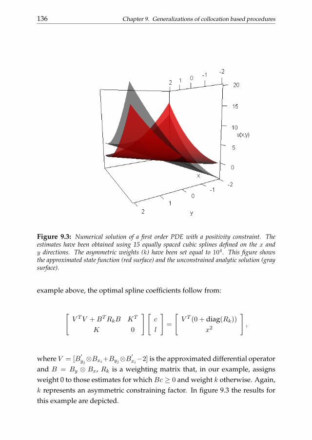
136 Chapter 9. Generalizations of collocation based procedures
Figure 9.3: Numerical solution of a first order PDE with a positivity constraint. Theestimates have been obtained using 15 equally spaced cubic splines defined on the x andy directions. The asymmetric weights (k) have been set equal to 104. This figure showsthe approximated state function (red surface) and the unconstrained analytic solution (graysurface).
example above, the optimal spline coefficients follow from:
[V TV +BTRkB KT
K 0
][c
l
]=
[V T (0 + diag(Rk))
x2
],
where V = [B′yj⊗Bxi+Byj⊗B
′xi−2] is the approximated differential operator
and B = By ⊗ Bx, Rk is a weighting matrix that, in our example, assignsweight 0 to those estimates for which Bc ≥ 0 and weight k otherwise. Again,k represents an asymmetric constraining factor. In figure 9.3 the results forthis example are depicted.
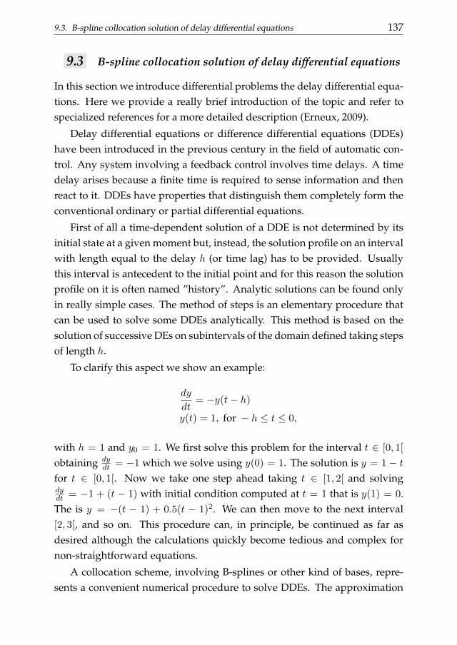
9.3. B-spline collocation solution of delay differential equations 137
9.3 B-spline collocation solution of delay differential equations
In this section we introduce differential problems the delay differential equa-tions. Here we provide a really brief introduction of the topic and refer tospecialized references for a more detailed description (Erneux, 2009).
Delay differential equations or difference differential equations (DDEs)have been introduced in the previous century in the field of automatic con-trol. Any system involving a feedback control involves time delays. A timedelay arises because a finite time is required to sense information and thenreact to it. DDEs have properties that distinguish them completely form theconventional ordinary or partial differential equations.
First of all a time-dependent solution of a DDE is not determined by itsinitial state at a given moment but, instead, the solution profile on an intervalwith length equal to the delay h (or time lag) has to be provided. Usuallythis interval is antecedent to the initial point and for this reason the solutionprofile on it is often named ”history”. Analytic solutions can be found onlyin really simple cases. The method of steps is an elementary procedure thatcan be used to solve some DDEs analytically. This method is based on thesolution of successive DEs on subintervals of the domain defined taking stepsof length h.
To clarify this aspect we show an example:
dy
dt= −y(t− h)
y(t) = 1, for − h ≤ t ≤ 0,
with h = 1 and y0 = 1. We first solve this problem for the interval t ∈ [0, 1[
obtaining dydt = −1 which we solve using y(0) = 1. The solution is y = 1 − t
for t ∈ [0, 1[. Now we take one step ahead taking t ∈ [1, 2[ and solvingdydt = −1 + (t − 1) with initial condition computed at t = 1 that is y(1) = 0.The is y = −(t − 1) + 0.5(t − 1)2. We can then move to the next interval[2, 3[, and so on. This procedure can, in principle, be continued as far asdesired although the calculations quickly become tedious and complex fornon-straightforward equations.
A collocation scheme, involving B-splines or other kind of bases, repre-sents a convenient numerical procedure to solve DDEs. The approximation
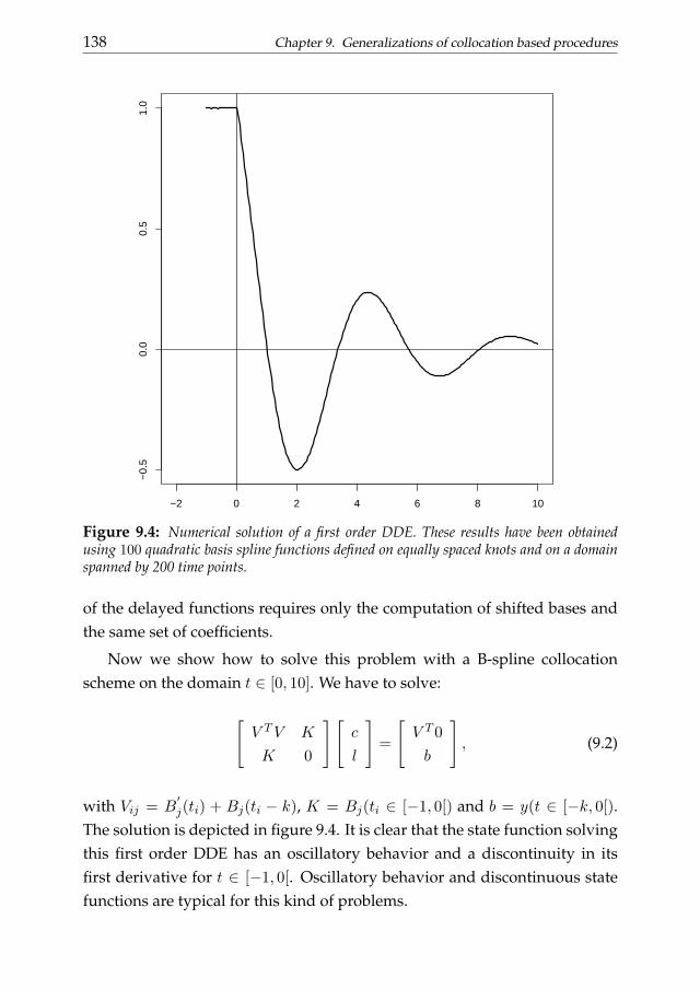
138 Chapter 9. Generalizations of collocation based procedures
−2 0 2 4 6 8 10
−0.
50.
00.
51.
0
Figure 9.4: Numerical solution of a first order DDE. These results have been obtainedusing 100 quadratic basis spline functions defined on equally spaced knots and on a domainspanned by 200 time points.
of the delayed functions requires only the computation of shifted bases andthe same set of coefficients.
Now we show how to solve this problem with a B-spline collocationscheme on the domain t ∈ [0, 10]. We have to solve:
[V TV K
K 0
][c
l
]=
[V T 0
b
], (9.2)
with Vij = B′j(ti) + Bj(ti − k), K = Bj(ti ∈ [−1, 0[) and b = y(t ∈ [−k, 0[).
The solution is depicted in figure 9.4. It is clear that the state function solvingthis first order DDE has an oscillatory behavior and a discontinuity in itsfirst derivative for t ∈ [−1, 0[. Oscillatory behavior and discontinuous statefunctions are typical for this kind of problems.
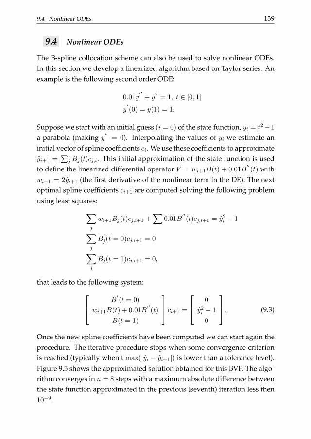
9.4. Nonlinear ODEs 139
9.4 Nonlinear ODEs
The B-spline collocation scheme can also be used to solve nonlinear ODEs.In this section we develop a linearized algorithm based on Taylor series. Anexample is the following second order ODE:
0.01y′′
+ y2 = 1, t ∈ [0, 1]
y′(0) = y(1) = 1.
Suppose we start with an initial guess (i = 0) of the state function, yi = t2−1
a parabola (making y′′
= 0). Interpolating the values of yi we estimate aninitial vector of spline coefficients ci. We use these coefficients to approximateyi+1 =
∑j Bj(t)cj,i. This initial approximation of the state function is used
to define the linearized differential operator V = wi+1B(t) + 0.01B′′(t) with
wi+1 = 2yi+1 (the first derivative of the nonlinear term in the DE). The nextoptimal spline coefficients ci+1 are computed solving the following problemusing least squares:∑
j
wi+1Bj(t)cj,i+1 +∑
0.01B′′(t)cj,i+1 = y2
i − 1
∑j
B′j(t = 0)cj,i+1 = 0
∑j
Bj(t = 1)cj,i+1 = 0,
that leads to the following system: B′(t = 0)
wi+1B(t) + 0.01B′′(t)
B(t = 1)
ci+1 =
0
y2i − 1
0
. (9.3)
Once the new spline coefficients have been computed we can start again theprocedure. The iterative procedure stops when some convergence criterionis reached (typically when t max(|yi − yi+1|) is lower than a tolerance level).Figure 9.5 shows the approximated solution obtained for this BVP. The algo-rithm converges in n = 8 steps with a maximum absolute difference betweenthe state function approximated in the previous (seventh) iteration less then10−9.
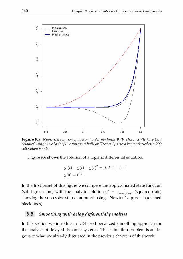
140 Chapter 9. Generalizations of collocation based procedures
0.0 0.2 0.4 0.6 0.8 1.0
−1.
2−
1.0
−0.
8−
0.6
−0.
4−
0.2
0.0 Initial guess
IterationsFinal estimate
Figure 9.5: Numerical solution of a second order nonlinear BVP. These results have beenobtained using cubic basis spline functions built on 50 equally spaced knots selected over 200collocation points.
Figure 9.6 shows the solution of a logistic differential equation.
y′(t)− y(t) + y(t)2 = 0, t ∈ [−6, 6]
y(0) = 0.5.
In the first panel of this figure we compere the approximated state function(solid green line) with the analytic solution y∗ = 1
1+exp(−t) (squared dots)showing the successive steps computed using a Newton’s approach (dashedblack lines).
9.5 Smoothing with delay differential penalties
In this section we introduce a DE-based penalized smoothing approach forthe analysis of delayed dynamic systems. The estimation problem is analo-gous to what we already discussed in the previous chapters of this work.
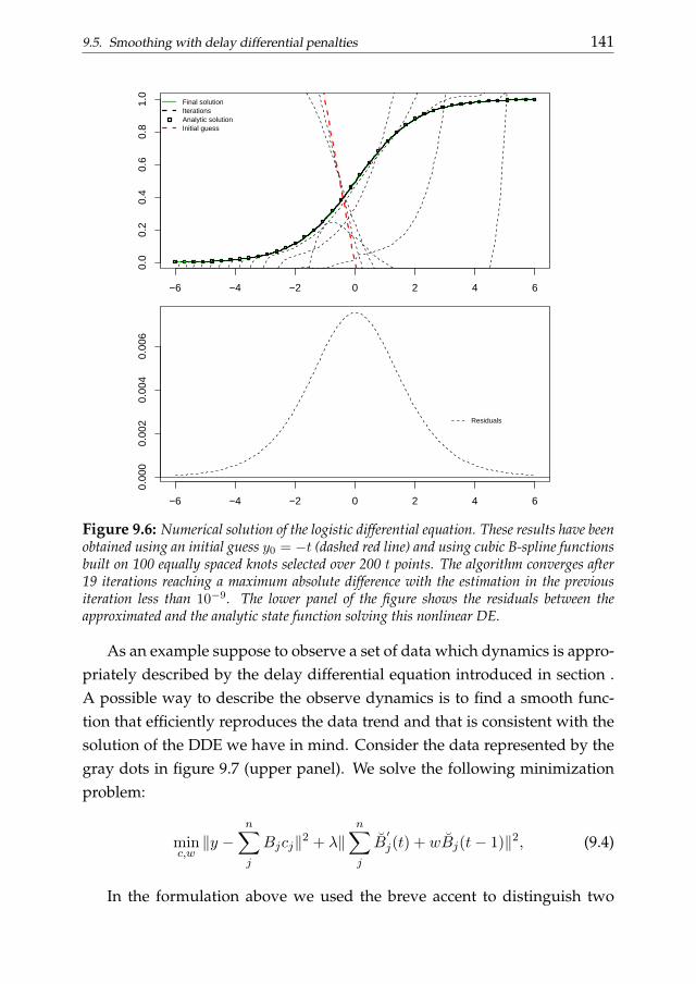
9.5. Smoothing with delay differential penalties 141
−6 −4 −2 0 2 4 6
0.0
0.2
0.4
0.6
0.8
1.0
xs
Final solutionIterationsAnalytic solutionInitial guess
−6 −4 −2 0 2 4 6
0.00
00.
002
0.00
40.
006
Residuals
Figure 9.6: Numerical solution of the logistic differential equation. These results have beenobtained using an initial guess y0 = −t (dashed red line) and using cubic B-spline functionsbuilt on 100 equally spaced knots selected over 200 t points. The algorithm converges after19 iterations reaching a maximum absolute difference with the estimation in the previousiteration less than 10−9. The lower panel of the figure shows the residuals between theapproximated and the analytic state function solving this nonlinear DE.
As an example suppose to observe a set of data which dynamics is appro-priately described by the delay differential equation introduced in section .A possible way to describe the observe dynamics is to find a smooth func-tion that efficiently reproduces the data trend and that is consistent with thesolution of the DDE we have in mind. Consider the data represented by thegray dots in figure 9.7 (upper panel). We solve the following minimizationproblem:
minc,w‖y −
n∑j
Bjcj‖2 + λ‖n∑j
B′j(t) + wBj(t− 1)‖2, (9.4)
In the formulation above we used the breve accent to distinguish two

142 Chapter 9. Generalizations of collocation based procedures
sets of points on which the basis functions are evaluated. The B-splines in-volved in the penalty term are evaluated on an ”enlarged” set of N collo-cation points. On the other hand the basis functions in B are evaluated atobserved domain points. This definition of the penalty term is convenient inthose cases where a moderate number of observations is available.
The parameter w is estimated using two-stage approach. In the first stagewe smooth the observations using a P-spline with an appropriate amount ofpenalty. Then, the optimal penalized coefficients can be used to approximatethe functions included in the differential penalty of (9.4). Once these approx-imated functions are obtained the optimal DE parameter can be computedusing least squares.
It is possible to notice that the DDE-based penalized smoothing estimatesare really close to the collocation approximation of the state function (seealso lower panel of figure 9.7). The optimal DE parameter has been foundapproximately equal to 1 (i.e. the value that we used to simulate the data). Avaluable feature is the reproduction of the discontinuity at t = 0.
9.6 Conclusions
In this chapter we have introduced some topics that will be part of our futureresearch.
Our discussion started with possible generalizations of the B-spline col-location scheme. First of all we have shown how to approximate the statefunction solving differential problems with nonconventional differential con-ditions. These conditions also have application in DE-based data smoothing.We could be interested, for example, in monotone smoothing applications orin smoothing data observed over irregular domains.
Then we introduced a collocation scheme for the solution of delayed dif-ferential equations which are common in many scientific fields studying dy-namic systems with feedbacks.
Furthermore we introduced a DDE-based penalized spline approach forthe analysis of observed phenomenon driven by delayed evolutions. In casedelayed dynamics, possible discontinuities in the state function call for a flex-ible smoothing approaches.
Finally, the collocation scheme has been adopted for the solution of non-
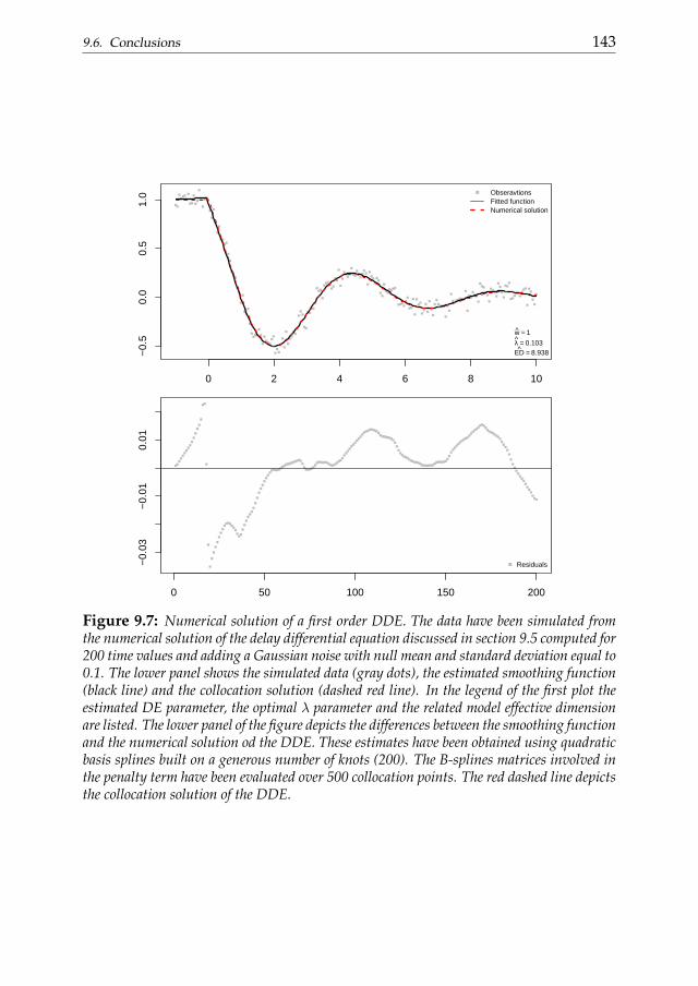
9.6. Conclusions 143
0 2 4 6 8 10
−0.
50.
00.
51.
0
x − 1
ObseravtionsFitted functionNumerical solution
w = 1
λ = 0.103ED = 8.938
0 50 100 150 200
−0.
03−
0.01
0.01
Residuals
Figure 9.7: Numerical solution of a first order DDE. The data have been simulated fromthe numerical solution of the delay differential equation discussed in section 9.5 computed for200 time values and adding a Gaussian noise with null mean and standard deviation equal to0.1. The lower panel shows the simulated data (gray dots), the estimated smoothing function(black line) and the collocation solution (dashed red line). In the legend of the first plot theestimated DE parameter, the optimal λ parameter and the related model effective dimensionare listed. The lower panel of the figure depicts the differences between the smoothing functionand the numerical solution od the DDE. These estimates have been obtained using quadraticbasis splines built on a generous number of knots (200). The B-splines matrices involved inthe penalty term have been evaluated over 500 collocation points. The red dashed line depictsthe collocation solution of the DDE.

144 Chapter 9. Generalizations of collocation based procedures
linear ODEs using an iterative linearization scheme.
CONCLUDING COMMENTS 10The aim of this thesis is to introduce advanced methods for of complexsmoothing problems. We mainly treat two aspects: the selection of the opti-mal weight of the roughness penalty and the definition of differential opera-tor penalty terms. Here we review shortly the topics treated in the previouschapters and introduce the directions of our future research.
With respect to the first topic, in chapter 3, we introduce the L-curvesmoothing parameter selection procedure. It selects the smoothing parame-ter through a direct comparison between the goodness of fit and the smooth-ness of the estimates. The optimal smoothing parameter can be selected bylocating the point of maximum curvature, i.e. the corner, of the L-curve aswas originally argued in the works of Hansen (Hansen, 1992; Hansen andO’Leary, 1993). We also propose an alternative selection procedure based onthe minimization of the Euclidean distance between the adjacent points ofthe curve: the V-curve criterion.
In chapter 4, the L-curve procedure is generalized to select the optimalamount of penalty in two-dimensional non-isotropic tensor product P-splinesmoothing. A natural two dimensional generalization of the L-curve is rep-resented by the L-surface, defined by a set of 1D L-curve computed in the xand y directions. Each L-curve has a convex region and the points definingthem become closer to each other in the proximity of the corner. The Eu-clidean distance between adjacent points on a single L-curve is described bya V-shaped curve and the single dimensional optimal smoothing parameteris located at the minimum of the V-curve.
In the next chapter we concentrate on smoothing procedures that use dif-ferential operator penalties. In particular we move from the introduction ofa B-spline collocation procedure for ordinary and partial differential equa-tions. As practical application we show how to solve the Black and Scholes
145
146 Chapter 10. Concluding comments
differential equation for pricing European options using a B-spline colloca-tion procedure.
In chapter 5, the B-spline collocation scheme an be adopted to definesmoothing procedures penalized by ordinary and partial differential opera-tors. In our approach the penalty term involves a combination of basis splinefunctions for the approximation of the differential operator in analogy with aB-spline collocation scheme. Penalizing the smoothing procedure by a lineardifferential operator consistency between the estimated smoothing functionand the state function approximating the solution of the DE-based penalty.Our aim can be viewed in terms of generalized differential conditions. Welook for a solution of the DE such to optimally describe the observed datain a least squares sense. On the other hand conventional initial/boundaryconditions as well as integral conditions can be included in the estimationprocedure through Lagrange multipliers.
A smoothing parameter regulates the fidelity of the final estimates to theapproximated state function. This parameter, if selected using an automaticprocedure, can be interpreted as a data-based measure of the appropriate-ness of the differential operator penalty. In particular we suggested to selectthis parameter through an EM-type algorithm exploiting the mixed modelinterpretation of penalized least squares.
In presence of unknown DE parameters we adopt a two stage estima-tion procedure: 1) smooth the raw data using a P-spline smoother able toremove the noise, 2) estimate the DE parameters through least squares. Thissimplification separates the computation of the DE parameters from the datasmoothing problem. The performance of this approach has been evaluatedwith simulated and real data.
In many applications, the data are grouped with respect to some factor.This leads to dynamic systems described by DEs with similar parameters. Inchapter 7, our DE-based penalized smoothing approach has been generalizedto take into account mixed DE parameters in one dimensional applications.In order to estimate the mixed effect model defining the DE hypothesized togovern the observed data we combine the two-stage P-spline-based proce-dure with a ridge regression framework. In this way we exploit the link be-tween penalized regression and mixed models (Pawitan, 2001). This allows apractical estimation and interpretation of the variance components. In mixed
10.1. Further research 147
models two variance parameters occur: one for the observation noise andone related to the random effects. Both can be estimated from the marginallikelihood, using an EM algorithm.
In the last chapter we introduce some topics that will be part of our futureresearch. We consider possible generalizations of the B-spline collocationscheme. We show how to approximate the state function solving differen-tial problems with inequality and shape constraints. An example is forcingthe numerical solution to be nonnegative or convex. Then we generalize theB-spline collocation framework for the solution of nonlinear ODEs and de-lay differential equations (DDEs) introducing also a DDE-based smoothingprocedure based on the same framework illustrated for the smoothing of dy-namic systems data described by ODEs and PDEs.
10.1 Further research
Our further research will develop in two directions and can be summarizedas follows:
• The first challenge we will face is related to the definition of a formalstatistical framework for the L-curve smoothing parameter selectionprocedure. Indeed, deeper studies on the non-statistical foundationsand interpretation of this selection procedure are needed. First of all itis of primary interest to give a formal explanation of its robustness tocorrelated noise. On the other hand we believe that a generalization ofthe L-curve (for one and two dimensional applications) for smoothingproblems with non Gaussian data and penalty terms defined by vectornorms different from the Euclidean one. Our future research will alsoconcentrate on an L-curve criterion for adaptive smoothing problemsand on L-curve suitable for expectile smoothing problems.
• A second line of research will be related to the B-spline collocationscheme. In particular we believe that the identification of the optimalcollocation points can represent an important issue in many applica-tions, especially dealing with observed data. Indeed, the accuracy ofthe approximation and the computational cost required by the colloca-tion scheme depend also on this aspect. In this work we adopt a ratherintuitive strategy locating the collocation points on a dense grid cover-
148 Chapter 10. Concluding comments
ing of the domain. The accuracy in terms of error analysis of our choicewas not investigated but it will be part of our future research.
• We will also focus on nonlinear DE-based penalized smoothing proce-dure. The requirement for linear differential penalties represents a biglimitation for the applicability of the procedures presented in this the-sis. A quasi-linearization Newton-type approach looks promising. Theintroduction of a nonlinear DE-based penalized smoothing approachcould represent an opportunity for a more appropriate description ofthe MRI-based stomach contractions analysis proposed in chapters 6and 7 of this thesis.
• In chapter 9 we proposed a DDE-based smoothing procedure show-ing a two-stage P-spline based procedure for the estimation of the un-known DDE parameters. We implicitly supposed to know the size ofthe delay h. In man application h is unknown and has to be estimatedfrom the data. The study of an appropriate procedure to estimate thedelay parameter will also be part of our further research.
• In this thesis, we supposed to observe data with exogenous source ofnoise. We did not deal with those circumstances in which the modelerrors are part of the dynamics. In this case modeling errors are intro-duced by systematic noise characterizing the differential model. Thisconsideration leads to the definition of stochastic differential basedpenalties in the smoothing settings. The differential operator penaliz-ing the smoothing procedure would represent the system noise in thesecases.
• Finally, an obvious subject would be to combine the L-curve procedureand differential operator penalties in a smoothing setting.
FORMAL DISCUSSION ABOUT THE SHAPE OF
THE L-CURVE AIt is possible to show some analytical results about the shape of the L-curve.These results can be useful to understand why, for well behaved curves, wecan simplify the selection procedure avoiding the computation of the cur-vature. In particular it is possible to show that the L-curve has a negativefirst derivative and that it has a convex region if some condition on the firstderivative of its components hold. We also show that if a convex area ex-ists the point of maximum curvature is well approximated minimizing theEuclidean distance between adjacent points on the curve.
In order to keep the mathematics as simple as possible let consider theWhittaker smoother even if our further reasoning can be generalized to othersmoothing procedures. In this case zλ = (I + λDTD)−1y represents the vec-tor of regularized fitted values (from this moment we will omit the hat andthe subscript symbols in order to simplify the notation). Plugging zλ in theexpressions for ω(λ) and θ(λ) we get:
ω(λ) = ‖y − (I + λP )−1y‖2
θ(λ) = ‖D(I + λP )−1y‖2.
where P = DTD.For our discussion it is necessary do determine the first derivative of z
with respect to λ. We can compute this derivative using implicit differentia-tion as follows:
y = (I + λP )z
0 = (I + λP )dz
dλ+ Pz
dz
dλ= −(I + λP )−1Pz.
Let H = (I + λP )−1 and differentiate ω and θ with respect to λ:
149
150 Appendix A. Formal discussion about the shape of the L-curve
dω
dλ=
(dω
dz
)T dzdλ
= −2(y − z)T dzdλ
= 2(zTPz − zTHPz)
= 2[zT (I −H)Pz]
= 2λzTPHPz, (A.1)
dθ
dλ=
(dθ
dz
)T dzdλ
= (2Pz)Tdz
dλ
= −2zTP THPz, (A.2)
and, given that P T = P , it is easy to notice that:
dω
dλ= −λdθ
dλ. (A.3)
From (A.3) we deduce that θ is a decreasing function of ω. Consideringrelation (A.3) we can analyze the convexity of the curve:
dω
dλ
dλ
dθ= −λ
dθ
dω= − 1
λd2θ
dω2=
d
dω
(− 1
λ
)=
(1
λ2
)dλ
dω
=
(λ2dω
dλ
)−1
=(2λ3zTP THPz
)−1. (A.4)
Equation (A.4) shows that the curve in normal scale is a convex function.As we said before the L-curve is defined in log-log scale. Let define the fol-lowing quantities:
ψ = log(ω); φ = log(θ),
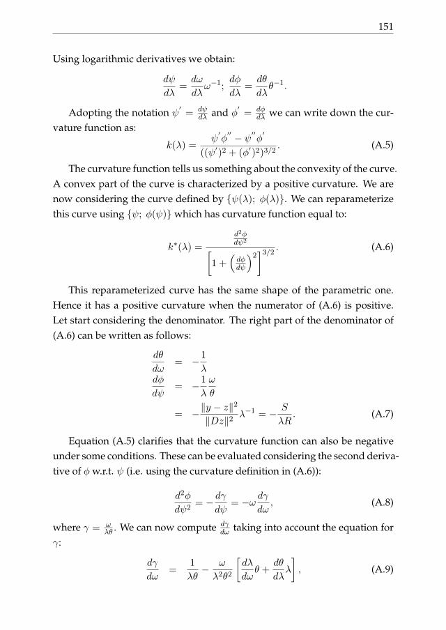
151
Using logarithmic derivatives we obtain:
dψ
dλ=dω
dλω−1;
dφ
dλ=dθ
dλθ−1.
Adopting the notation ψ′
= dψdλ and φ
′= dφ
dλ we can write down the cur-vature function as:
k(λ) =ψ′φ′′ − ψ′′φ′
((ψ′)2 + (φ′)2)3/2. (A.5)
The curvature function tells us something about the convexity of the curve.A convex part of the curve is characterized by a positive curvature. We arenow considering the curve defined by ψ(λ); φ(λ). We can reparameterizethis curve using ψ; φ(ψ)which has curvature function equal to:
k∗(λ) =
d2φdψ2[
1 +(dφdψ
)2]3/2
. (A.6)
This reparameterized curve has the same shape of the parametric one.Hence it has a positive curvature when the numerator of (A.6) is positive.Let start considering the denominator. The right part of the denominator of(A.6) can be written as follows:
dθ
dω= − 1
λdφ
dψ= − 1
λ
ω
θ
= −‖y − z‖2
‖Dz‖2λ−1 = − S
λR. (A.7)
Equation (A.5) clarifies that the curvature function can also be negativeunder some conditions. These can be evaluated considering the second deriva-tive of φ w.r.t. ψ (i.e. using the curvature definition in (A.6)):
d2φ
dψ2= − dγ
dψ= −ω dγ
dω, (A.8)
where γ = ωλθ . We can now compute dγ
dω taking into account the equation forγ:
dγ
dω=
1
λθ− ω
λ2θ2
[dλ
dωθ +
dθ
dλλ
], (A.9)

152 Appendix A. Formal discussion about the shape of the L-curve
but we know that dθdλ = − 1
λ and dλdφ = −θ dλdωλ. So we can write equation (A.9)
as follows:dγ
dω=
1
λθ− ω
λ2θ2
[− 1
λ
dλ
dφ− 1
]. (A.10)
The numerator of the curvature function (A.6) is then equal to:
d2φ
dψ2=dφ
dψ+
(dφ
dψ
)2 [− 1
λ
dλ
dφ− 1
]. (A.11)
The L-curve procedure suggests to locate the optimal smoothing param-eter in the point of maximum curvature. For this reason it is convenient tofind a condition for which d2φ
dψ2 assumes positive values. Given that dφdψ < 0,
in order to have a positive curvature the following inequality has to hold:(dφ
dψ
)2 [− 1
λ
dλ
dφ− 1
]> −dφ
dψ
dφ
dψ
[− 1
λ
dλ
dφ− 1
]< −1
− 1
λ
dλ
dφ> −dψ
dφ+ 1
− 1
λ
dλ
dφ>−dψ + dφ
dφ1
λdλ > dψ − dφ. (A.12)
Differentiating both sides of (A.12) w.r.t. λ and considering that ψ and φ
are in log scale and that dλλ = d log(λ) we get the final relation (considering
log(λ) = `):
1 >dψ
d`− dφ
d`. (A.13)
This condition can be verified numerically. Consider as examples twocases showed above. In particular we take a case in which a clear corner ispresent and another in which the convex region of the L-curve is not pro-nounced. The first case is given by the example in figure 3. Figure A.1 showsthe curvature function related with this example. The smaller segments un-der this curve show the positive curvature points found using (A.13). Thesecond panel of figure A.1 plots the numerator of the curvature function andthe vertical lines indicate the points of positive curvature found applying thecriterion in (A.13). On the other hand figure A.2 shows the results obtained
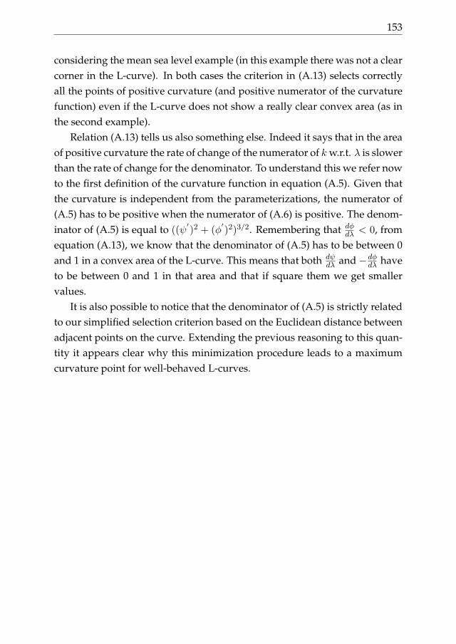
153
considering the mean sea level example (in this example there was not a clearcorner in the L-curve). In both cases the criterion in (A.13) selects correctlyall the points of positive curvature (and positive numerator of the curvaturefunction) even if the L-curve does not show a really clear convex area (as inthe second example).
Relation (A.13) tells us also something else. Indeed it says that in the areaof positive curvature the rate of change of the numerator of k w.r.t. λ is slowerthan the rate of change for the denominator. To understand this we refer nowto the first definition of the curvature function in equation (A.5). Given thatthe curvature is independent from the parameterizations, the numerator of(A.5) has to be positive when the numerator of (A.6) is positive. The denom-inator of (A.5) is equal to ((ψ
′)2 + (φ
′)2)3/2. Remembering that dφ
dλ < 0, fromequation (A.13), we know that the denominator of (A.5) has to be between 0and 1 in a convex area of the L-curve. This means that both dψ
dλ and −dφdλ have
to be between 0 and 1 in that area and that if square them we get smallervalues.
It is also possible to notice that the denominator of (A.5) is strictly relatedto our simplified selection criterion based on the Euclidean distance betweenadjacent points on the curve. Extending the previous reasoning to this quan-tity it appears clear why this minimization procedure leads to a maximumcurvature point for well-behaved L-curves.
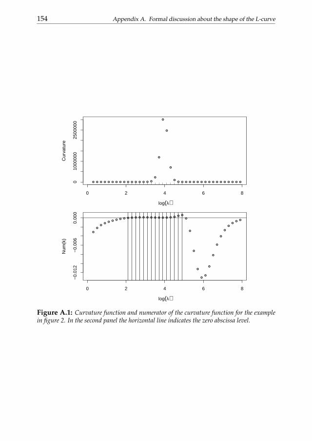
154 Appendix A. Formal discussion about the shape of the L-curve
0 2 4 6 8
010
0000
025
0000
0
log(λ)
Cur
vatu
re
0 2 4 6 8
−0.
012
−0.
006
0.00
0
log(λ)
Num
(k)
Figure A.1: Curvature function and numerator of the curvature function for the examplein figure 2. In the second panel the horizontal line indicates the zero abscissa level.
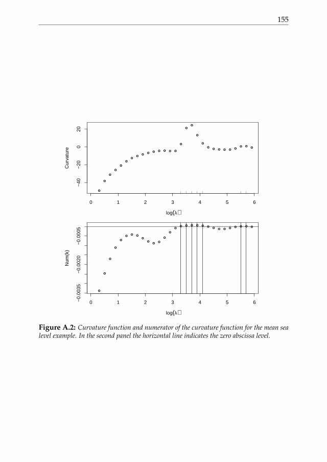
155
0 1 2 3 4 5 6
−40
−20
020
log(λ)
Cur
vatu
re
0 1 2 3 4 5 6−0.
0035
−0.
0020
−0.
0005
log(λ)
Num
(k)
Figure A.2: Curvature function and numerator of the curvature function for the mean sealevel example. In the second panel the horizontal line indicates the zero abscissa level.

BIBLIOGRAPHY
Ascher, U. M. and Petzold, L. R. (1998). Computer Methods for Ordinary Dif-ferential Equations and Differential-Algebraic Equations. Society for Industrialand Applied Mathematics, Philadelphia, PA, USA, 1st edition.
Belge, M., Kilmer, M., and Miller, E. L. (1998). Simultaneous multiple regu-larization parameter selection by means of the l-hypersurface with appli-cations to linear inverse problems posed in the wavelet transform domain.
Black, F. and Scholes, M. (1973). The pricing of options and corporate liabili-ties. Journal of Political Economy, 81(3):637–654.
Botella, O. (2002). On a collocation B-spline method for the solution of theNavier–Stokes equations. Computers and Fluids, 31(4-7):397–420.
Cao, J. and Ramsay, J. O. (2007). Parameter cascades and profiling in func-tional data analysis. Comput. Stat., 22(3):335–351.
Carmack, P. S., Spence, J. S., and Schucany, W. R. (2012). Generalised corre-lated cross-validation. Journal of Nonparametric Statistics, 24(2):269–282.
Coddington, E. A. and Levinson, N. (1984). Theory of Ordinary DifferentialEquations. Robert E. Krieger, Malabar, Florida.
Cox, J. C., Ross, S. A., and Rubinstein, M. (1979). Option pricing: A simplifiedapproach. Journal of Financial Economics, 7(3):229–263.
Currie, I. D. and Durban, M. (2002). Flexible smoothing with P-splines: aunified approach. Statistical Modelling, 4:pp. 333–349.
de Boor, C. (1978). A Practical Guide to Splines. Springer-Verlag.
de Boor, C. and Swartz, B. (1973). Collocation at Gaussian Points. SIAMJournal on Numerical Analysis, 10(4).
157
158 Bibliography
Dierckx, P. (1995). Curve and Surface Fitting with Splines. Oxford UniversityPress.
Eilers, P., Currie, I., and Durban, M. (2006). Fast and compact smoothingon large multidimensional grids. Computational Statistics & Data Analysis,50(1):61–76.
Eilers, P. H. (2003). A perfect smoother. Analytical chemistry, 75(14):3631–3636.
Eilers, P. H. C. and Marx, B. D. (1996). Flexible smoothing with B-splines andpenalties. Statistical Science, 11(2):pp. 115–121.
Eilers, P. H. C. and Marx, B. D. (2003). Multivariate calibration with tem-perature interaction using two-dimensional penalized signal regression.Chemometrics and Intelligent Laboratory Systems, 66:159–174.
Eilers, P. H. C. and Marx, B. D. (2010). Splines, knots, and penalties. WileyInterdisciplinary Reviews: Computational Statistics, 2(6):637–653.
Erneux, T. (2009). Applied Delay Differential Equations. Surveys and tutorialsin the applied mathematical sciences. Springer-Verlag New York.
Evans, L. C. (1998). Partial Differential Equations (Graduate Studies in Mathe-matics, V. 19) GSM/19. American Mathematical Society.
Golub, G. H. and Ortega, J. M. (1992). Scientific Computing and DifferentialEquations. Academic Press, New York and London.
Hansen, P. C. (1992). Analysis of Discrete Ill-Posed Problems by Means of theL-curve. SIAM Review, 34(4):pp. 561–580.
Hansen, P. C. (2000). The L-curve and its use in the numerical treatment ofinverse problems. In Computational Inverse Problems in Electrocardiology, ed.P. Johnston, Advances in Computational Bioengineering, pages 119–142. WITPress.
Hansen, P. C. and O’Leary, D. P. (1993). The use of the L-Curve in the regu-larization of discrete ill-posed problems. SIAM J. SCI. COMPUT., 14(6):pp.1487–1503.
Bibliography 159
Hastie, T. J. and Tibshirani, R. J. (1990). Generalized additive models. London:Chapman & Hall.
Hodrick, R. J. and Prescott, E. C. (1997). Postwar U.S. Business Cycles: AnEmpirical Investigation. Journal of Money, Credit and Banking, 29(1):pp. 1–16.
Johns, C., Nychka, D., T.G.F., K., and Daly, C. (2003). Infilling sparse recordsof spatial fields. Journal of the American Statistical Association, 98:796–806.
Kauermann, G., Krivobokova, T., and Semmler, W. (2011). Filtering time se-ries with penalized splines. Studies in Nonlinear Dynamics & Econometrics,15(2):2.
Krivobokova, T. and Kauermann, G. (2007). A note on penalized splinesmoothing with correlated errors. Journal of the American Statistical Asso-ciation, 102:1328–1337.
Marx, B. D. and Eilers, P. H. (2005). Multidimensional penalized signal re-gression. Technometrics, 47(1):13–22.
Pandit, S. M. and Wu, S. M. (1993). Time series and system analysis with applica-tions. Krieger.
Pawitan, Y. (2001). In All Likelihood: Statistical Modelling and InferenceUsing Likelihood.
Ramsay, J. O. and Silverman, B. W. (2005). Functional Data Analysis. SpringerSeries in Statistics. Springer, 2nd edition.
Ramsay, T. (2002). Spline smoothing over difficult regions. Journal of the RoyalStatistical Society: Series B (Statistical Methodology), 64(2):307–319.
Ruppert, D., W. M. C. R. (2003). Semiparametric Regression. Cambridge Seriesin Statistical and Probabilistic Mathematics (No. 12).
Schall, R. (1991). Estimation in generalized linear models with random ef-fects. Biometrika, 78(4):719–727.
Schumaker, L. L. (1981). Spline Functions: Basic Theory. John Wiley and Sons,New York.
160 Bibliography
Shahrak, N. M., S. A. O. (2013). Robust psd determination of micro and meso-pore adsorbents via novel modified u curve method. Chemical EngineeringResearch and Design, 1(91):51–62.
Stock, J. and Watson, M. (2003). Introduction to econometrics. The Addison-Wesley series in economics. Addison-Wesley, Boston, Mass. [u.a.], internat.ed edition.
Vogel, C. R. (1996). Non-convergence of the l-curve regularization parameterselection method. Inverse Problems, 12(4):535.
Wahba, G. (1990). Spline models for observational data, volume 59 of CBMS-NSFRegional Conference Series in Applied Mathematics. Society for Industrial andApplied Mathematics (SIAM), Philadelphia, PA.
Wang, L., Cao, J., Ramsay, J. O., Burger, D. M., Laporte, C. J. L., and Rock-stroh, J. K. (2012). Estimating mixed-effects differential equation models.Statistics and Computing, pages 1–11.
Welham, S. J., Cullis, B. R., Kenward, M. G., and Thompson, R. (2006). Theanalysis of longitudinal data using mixed model l-splines. Biometrics,62(2):392–401.
Welham, S. J. and Thompson, R. (2009). A note on bimodality in the log-likelihood function for penalized spline mixed models. Comput. Stat. DataAnal., 53:920–931.
Whittaker, E. T. (1922). On a new method of graduation. Proceedings of theEdinburgh Mathematical Society, 41:63–75.
Wood, S. N., Bravington, M. V., and Hedley, S. L. (2008). Soap film smoothing.Journal Of The Royal Statistical Society Series B, 70(5):931–955.