universal smoothing factor selection in density...
TRANSCRIPT

Sociedad de Estad(stica e Investigacidn Operativa Test (1997) Vol. 6, No. 2, pp. 223-320
Universal smoothing factor selection in density estimation" theory and practice L u c D e v r o y e
School of Computer Science, McGill University Montreal, Canada H3A 2K6. [email protected]
A b s t r a c t
In earlier work with Gabor Lugosi, we introduced a method to select a smoothing factor for kernel density estimation such that, for all densities in all dimensions, the L1 error of the corresponding kernel estimate is not larger than 3 + e times the error of the estimate with the optimal smoothing factor plus a constant times Ov~--~-n/n, where n is the sample size, and the constant only depends on the complexity of the kernel used in the estimate. The result is nonasymptotic, that is, the bound is valid for each n. The estimate uses ideas from the minimum distance estimation work of Yatracos. We present a practical implementation of this estimate, report on some comparative results, and highlight some key properties of the new method.
K e y W o r d s : Density estimation, kernel estimate, convergence, smoothing factor, minimum distance estimate, asymptotic optimality, simulation study.
A M S s u b j e c t c l a s s i f i c a t i o n : 62G05.
1 I n t r o d u c t i o n
W e a r e g i v e n an i . i .d , s a m p l e X 1 , . . . , X ~ d r a w n f r o m a n u n k n o w n d e n s i t y
f on ]R d, a n d c o n s i d e r t h e A k a i k e - P a r z e n - R o s e n b l a t t d e n s i t y e s t i m a t e
f h(x) = a ' h ( X - i= l
where K : IR d --+ lR is a fixed kernel with f K = l, Kh(x) = (1/hd)K(x/h) , and h > 0 is the smoothing factor (Akaike, 1954; Parzen, 1962; Rosenblatt, 1956). In this paper, we focus on density estimation without restrictions on the densities. The fundamental problem in kernel density estimation is that of the joint choice of h and K in the absence of a priori information regarding f . Watson and Leadbetter (1963) show that the choice of h and K should not be split into two independent subproblems. Also, the choice
The author 's work was supported by NSERC Grant A3456 and by FCAR Grant 90-ER-0291.

224 L. Devroye
of K largely depends upon the smoothness of f . However, the choice of K will only be of secondary interest in this paper.
All global smoothing factors can be written in the general form H = H~(X1, . . . ,Xn). A selection method is thus nothing but a sequence of fufictions {H~, n >_ 1}. If we let jr denote the class of all densities o n IR d, and let f~H denote a kernel estimate with data-based bandwidth H, we look at
limsup E f If,~H - flf[ s sup inV. - -
and its non-asymptotic counterpart
E f [fnH - - f[ sup Se~- infh E f [fnh - fl
The boundedness of these suprema shows that the bandwidth selector works well for all f , without exception.
Recently, Devroye and Lugosi (1996) introduced a data-dependent smooth- ing factor H for which
E f iAi_ t - flf[ suplimsupy n - ~ in~hEf[-fn-h --- < 3 ,
whenever the kernel K is nonnegative, Lipschitz, and of compact support. The estimate of that paper requires various parameter choices which in turn are used to define the procedure for finding H. A related estimate was proposed in Devroye and Lugosi (1997) that comes with explicit non- asymptotic performance guarantees. Both estimates will be revisited in this paper.
We define various classes of bandwidth selectors as follows:
A. UNIVERSALLY CONSISTENT BANDWIDTHS. Bandwidths for which for all f ,
lim E / I f r i l l - f 1 = 0 $
n - - ~ o o J
Bandwidths that are not universally consistent are called inconsistent.
B. SUITABLE BANDWIDTHS. Bandwidths for which for all f ,
E f - f l lim sup n-~o~ infh E f [f~h -- f[
< c(f) <

Universal smoothing .factor 225
for some finite constant C(f) . Bandwidths outside this class are said to be unsuitable.
C. UNIVERSALLY SUITABLE BANDWIDTHS. Suitable bandwidths for which the constant C(f ) is universally bounded for all f . Smoothing factors not in this class are called "not universally suitable".
D. ASYMPTOTICALLY OPTIMAL BANDWIDTHS. Suitable bandwidths for which for all f , C( f ) = 1.
One can classify bandwidths into one of the four nested classes. We are interested in this paper in universally suitable bandwidths for all dimensions d. We will therefore only briefly review bandwidths that are not in this class. More complete surveys may be found in Devroye and GySrfi (1985), Marron (1987, 1988, 1989a), Izenman (1991), Jones, Marron and Sheather (1992), Park and Turlach (1992), Titterington (1985), Turlach (1993), Cao, Cuevas and Gonzs (1994), Berlinet and Devroye (1994), and Wand and Jones (1995).
A S Y M P T O T I C A L O P T I M A L I T Y AND AN OPEN P R O B L E M . We will n o t fo-
CUS on asymptotically optimal bandwidths, simply because we do not know if this class is nonempty. This remains one of the most compelling open problems in the field. It should be noted however that there are many pub- lished bandwidths that are asymptotically optimal for given subclasses. For example, if f is restricted to a class of univariate densities in which only a translation and scale parameter is unknown, using h -- a , ~ for a func- tion a,~ (depending upon the family), where ~ is a data-based estimate of the scale factor, will do (see Deheuvels (1977a, 1977b) or Deheuvels and Hominal, 1980). The smoothing factor h can also be based upon a plug-in of estimates of unknown functionals into a given formula. This method has the given property if the supremum is taken over classes of univariate densities restricted by smoothness and small tails (Hall and Wand, 1988). The double kernel estimate (Devroye, 1989) satisfies the property men- tioned above when the supremum is restricted as in the work of Hai land Wand. Except for trivially restricted classes of densities, none of the L2 cross-validated estimates in the literature (see Rudemo (1982), Bowman (1984) or Stone (1984) for the early papers on this) possesses the property mentioned above.

226 L. Devroye
RELATED KERNEL ESTIMATES. It is necessary to limit the scope of the paper. We are deliberately not considering local bandwidth selectors or variable kernel methods, although some of these have proven track records. One should also keep in mind that we may always transform the data, apply a fixed kernel est imate such ms the estimates discussed in this paper, and then retransform the kernel estimate (see chapter 9 of Devroye and GySrfi, 1985). This has the effect of introducing variable bandwidths.
2 T h e f i r s t b a n d w i d t h
Split the da ta set into a test set of size m ~< n and a remainder. The first bandwidth of Devroye and Lugosi (1996) uses Yatracos' minimum distance projection of the empirical measure based upon these m points to the class of densities defined by the kernel estimates based on the remaining n - m points to find an optimal h (Yatracos, 1985). This is at tractive because it directly relates a density estimate to the s tandard empirical measure.
Let m < n be a positive integer, let K be a nonnegative kernel with f K(x)dx = 1, and let ~'n be the class of densities
n - - m
fn:m,h(X)- 1 ~ Kh(X- Xi) n - - m
i=1
with h E [an, bn], where the nonnegative numbers an, bn will be specified later such that the optimal smoothing factor eventually falls in [an, bn] for all densities. Next we cover the class ~'n by finitely many densities as follows: let (f n > 0 be a parameter to be specified later, let hi : an, and hi = hi_l(1 + 5n) for all i -~ 2 , . . . , N, where N is the largest integer with an(1 + ~n) N - I ~_ bn. The finite class of densities {fn-m,h, : i = 1, . . . , N) is denoted by ~n. Our est imate will be drawn from this finite class!
Let #m be the empirical measure defined by the rest of the da ta points: X n - m + l , . . . ,X~, i.e., for any Borel set A C_ IR d,
1 n
= - IA(X,), urn(A) m i=n--m+l
where IA denotes the indicator function of A. As is well-known, the L1 distance is equivalent to the twice the total variation distance. If we are to

Universal smoothing factor 227
use the empirical measure, we would thus be tempted to select h so as to minimize the total variation
T de----fSUPA fA f n - m ' h - - # m ( A ) l "
As #m is an atomic measure, T = 1 for all h. Following a clever idea of Yatracos (1985), we take the supremum instead over a specially picked rich class of subsets .4, defined as the family of sets
{x : .f~-m,h~(x) > fn-m,h~(x)}, i , j <_ N.
The est imate fn is defined to be that fn-,~,h, E ~,~ for which
sup fA fn-m,h, -- #m(A) AEA
is minimal. If the minimum is not unique, we choose among the minimizing densities according to a prespecified rule, e.g., we choose the one with smallest index. Note that in any case, our est imate optimizes over a given finite set, and is thus defined with computional efficiency in mind.
~} CHOICE OF THE PARAMETERS. It helps at this stage to pin down choices for a~, bn and 5n. The choice is determined by the choice of the kernel K. We assume the following: a kernel is said to be elegant if it is nonnegative, if it is Lipschitz of constant C (i.e., I g ( x ) - K(y)I <_ CIIx - Yll for all x ,y) , and if K = 0 outside [ -1 , 1] d. Then define an = e -n, bn = e n, 5n = c / x /~ for a fixed constant c. This class contains the s tandard Deheuvels kernel tha t is optimal in IR d and is of the form C'(1 - I Ix l ld)+, where (u)+ = max(u, 0). For more general classes, we will show how to take the parameters in remarks below.
0 A COMPUTATIONAL REMARK. In most univariate cases, the sets A above are finite unions of intervals. The number of such intervals can be rigorously controlled if the kernel is polynomial on a compact set (such as with the celebrated Epanechnikov-Bartlet t kernel 3/4(1 - x 2 ) + ) . The computat ions are much more involved for d > 1, unless K is the indicator function of a unit square. The class .,4 has N 2 members. A quick calculation shows that
log(bn/an) n(2 + ~n) N - 1 _< log(1 + ~,,) -< 6n
-- n + 2n3/2/c .

228 L. Devroye
A lower bound on the number of integrals over sets A (if we were to naively minimize) would be of the order of n 3. However, clever shortcuts are pos- sible.
THE SET ,4. The set ,4 cannot be replaced by the set of all rectangles of IR d. This class is simply not rich enough, and Lemma 2 below would not be valid.
T h e o r e m 2.1. (Devroye and Lugosi, 1996). Let K be an elegant kernel.
Let an, bn be such that na,~ --+ 0 and bn --+ oo. A s s u m e that 5,~ = c / v ~ for some cons tant c and that l o g ( b J a n ) < cln a for some f ini te c I, a > O. I f
m m - - - + 0 and ~ oo as n - + oo, n n4/5 log n
then the es t imate f,~ defined above satisfies
E f IA - fl sup lira sup f ,,~o~ i n f h E f l A , h - - f l <3"
This result is valid for any multivariate density. It may be possible to improve the constant in the bound. With a bit of work, one may also be able to replace f~ in the result by fnH, where H is the smoothing factor used in fn- The difference here is that f n H u s e s all n da ta points, while fn is the kernel est imate based on H and X 1 , . . . , Xn-,~.
One may argue that the selected smoothing factor is not scale-invariant. This is easily taken care of by letting Mn denote the median of the (~2 TM) distances ]]Xi - Xj]], 1 <_ i , j <_ n - m, and setting a,~ = Mne -n and bn = M,~e ~. As M,~ is almost surely bounded away from 0 and infinity, one can verify that the Theorem holds for this choice of interval.
For convenience we assumed tha t the kernel K is nonnegative. It is well known, however, tha t some kernels taking negative values provide smaller L1 errors for smooth densities. The above theorem is easily extended" to such kernels at the expense of further restrictions on the growth of m, depending on the order of the kernel.
Finally, there is quite a bit of freedom in the choice of all the parameters. For example, 5n does not have to tend to zero at the rate 1/v/-n. A practical implementation is described in the next section.

Universal. smoothing factor 229
The universality of Theorem 2.1 can only be achieved thanks to combi- natorial arguments. Error analysis based on Taylor series expansions of f are simply out of the question, as such expansions may not exist. For the proof of Theorem 2.1, we refer to Devroye and Lugosi (1996a). However, we will s ta te four lemmas, which each contribute key elements to the proof.
L e m m a 2.1. (Devroye and Lugosi, 1996). For each density f and elegant kernel K, C' = c2dv/-d + d, the estimate fn(E Gn) satisfies
I f . - f l < 3 inf I f . - m , h - f l + + 4 s u p - f �9 - he[an,bn] ~ AeA
The middle term accounts for a Lipschitz effect between nearby kernel estimates. The last term resembles a total variation distance between an empirical measure and a density. If .A were the class of all Borel sets, this term would take the value 4. Fortunately, ,4 is finite, so that we may bound the expected value of the last term by
8v/log c" + (2a + 1) logn + 1
provided log(bJa, ) <_ c'n a for positive constants c ' ,a . Thus, the right hand side in Lemma 1 is easily bounded. Now the range outside [a,, b,] is uninteresting because of the following result (a version in which h is a random variable is given by Broniatowski, Devroye and Deheuvels, 1989).
L e m m a 2.2. (Devroye, 1983). Assume K >_ O. If E f [ f , h - fl -'+ 0 for some density f and some sequence h, then h -+ 0 and nh d --+ cx). Conversely, if h -+ 0 and nh d -4 oc, then E f ]fnh - f] --+ 0 for all densities
f .
Finally, the ratio result in Theorem 2.1 follows from the following two lemmas.
L e m m a 2.3. (Devroye and Penrod, 1984). Assume K >_ O. Then
g
inf lim inf n 2/5 inf E / Ifnh -- f l > 0.86. ] n-+cr h J
We note tha t Lemma 2.3 was only proved in the cited paper for d = 1. However, if f and fnh a r e a density and a kernel density est imate on IR d,

230 L. Devroye
and if g and gnh denote the marginal densities for f and f~h (with respect to any fixed component) , then,
E / 'gnh -- g' <_ E / 'f,~h -- f '
(Devroye and GySrfi, 1985). Interestingly, gnh itself is a valid univariate kernel est imate with as kernel the marginal density of the original kernel. Therefore, a universal lower bound for d = 1 of the type shown in Lemma 5 then applies equally for all dimensions d.
L e m m a 2.4. (Devroye and Lugosi, 1996). Let K be a bounded kernel. Define
= J If h - II @
If m > 0 is a positive integer such that 2m <_ n, then
in fhEJn-m,h <_ 1 + 2m + 8, [-m 1 _< infhEJn,h n~--m V n "
Theorem 2.1 deals with f~ = fn-m,H, not f n H . In other words, the est imate does not use the full sample. In fact, in Theorem 2.1, we may replace f~ by f~H without harm.
3 A n i m p l e m e n t a t i o n o f t h e f i r s t b a n d w i d t h
For one-dimensional densities, we propose a practical implementation. With- out loss of generality, we consider the Epanechnikov-Bartlet t kernel K(x) = ( 3 / 4 ) ( 1 - x2)+. Our method (with bandwidth called hdl) has the following parameter settings:
m A. m -- [n~ Note that ~ -+ oc as required. For n = 100, m = 50.
B. t - 1.5: t > 1 is a threshold to be discussed further on. As t ap- proaches 1, the algorithm slows down but will give increasingly accu- rate results.
C. k = 10: k is the number of intervals considered in a global search for the optimum.

Universal smoothing factor 231
The algorithm may be described in a few steps:
.
.
.
Split the da ta into two sets, A' and Y, where A' = (X1 , . . . , Xn-r , ) and y = (X ,~ -m+l , . . . ,Xn ) .
Compu te h and H: h is the minimum distance between consecutive
points in X, H = X(f3(~-m)/41) - X([(,~-m)/4J), and X(j) is the j - th smallest of the values in A'. Observe tha t h < H, and tha t for n - m large enough, the optimal bandwidth is almost surely in the range [h, H]. Define ~* = hv/-h-H. Define T = U/h.
While T > t do:
3.1. Define ~ = T 1/k. Let 7/ be the set of k + 1 candidate bandwidths h~ i for 0 < i < k. Observe that the first and last bandwidths are h and H respectively.
3.2. For all ~ r ( ' �9 7/ compute A(~,~') = {fn-m,~ > f,~-m,~'}- The collection of these sets is called .4. Observe that IAI = k(k - 1).
1 3.3. For all ~ �9 7/ compute J(~) = maxaEA Ira fn-m,~ -- "~ E x E y I*ea l" 3.4. Let ~* be that value in 7/for which J(~) is minimal.
3.5. Set (h,H) = (~*/(f,~*~). Set T = $2.
4. Return ~*.
The choice of the parameters is motivated by computat ional considera- tions. Assume a nice unimodal density with peak value M and with spread
a, where spread is measured as the difference between third and first quar- tiles. Then h is of the order of 1 / ( M n 2) and H is initially close to a, so tha t at the outset, T ,~ a M n 2. After i iterations, we have T ~ (aMn2) 2i/k. We stop as soon as this drops below the threshold t. This occurs roughly when
k log(t) i ~ - •
2 log(aMn 2) "
The influence of a M is moderated by a logarithm. For the uniform density, a M = 1/2. If we fill in the other parameter choices and set n = 100, we obtain
5 log 1.7
log 5000 '
tha t is, i ,~ 0.31. In fact, it is likely that only one while loop is executed, which in turn requires computation proportional to k'2n because IAI =

232 L. Devroye
k(k + 1)/2 and because each integral takes time bounded by n if the da ta are storedproperly. Discounting the dependence upon the distribution, the time grows roughly as
k 2 n m a x ( i , l o g ~ ) �9
Taking k very small does help, but reduces the quality of the solution, as the optimization is done over a rougher grid.
4 T h e s e c o n d b a n d w i d t h
The second bandwidth of Devroye and Lugosi (1997) does not use a finite interval [an, b,~] for the optimization, and thus eliminates the need to pick these parameters. The second difference is that the class .A is infinite. This eliminates the need for a third parameter, 5,,, but renders the optimization a bit more problematic. Introduce the class /~k of kernels of the form
k
= i=1
where IA denotes the indicator function of a set A, k < oc, ~1, �9 �9 �9 , ~k E ]R, and A I , . . . , Ak are Borel sets in IR d with the following property: the intersection of an infinite ray {x : x -- txo, t _> 0}, anchored at the origin, with any Ai is an interval. Examples of such A~s include all convex sets and all star-shaped sets (a set A is star-shaped if x E A implies Ax E A for all )~ E [0, 1]). The Ai's need not be disjoint. However, if the Ai's are disjoint rectangles, the sum looks a bit like a Riemann approximation of a function. Thus, kernels of the type given here are called Riemann kernels of parameter k. Denote the class of all such functions by T~k. The most important examples include the uniform densities on ellipsoids, balls, and hypercubes.
We first select k and K ~ E/~k such that
f lK - K'l _< 1 - - .
7~
Note that this is always poasible if K is Riemann integrable. The size k as a function of n will be discussed further on. A kernel est imate with kernel K ~ is piecewise constant and thus easy to work with in simulations.

Universal smoothing factor 233
The second and last choice is that of a parameter m <_ n/2 tha t will be used to split the da ta set into a small test set of size m and a large main sample of size n - m. Define the kernel est imates
n - - m
, _ _I ~ KIh(X- X~) ( x ) n m
i=l
for all h > 0. Let #m be the empirical measure defined by the rest of the da ta points: Xn-m+l , . . . , X,~, tha t is, for any Borel set A C_ IR d,
#re(A) = --i ~ IA(Xi). m .
~ = n - m + l
Let H be that smoothing factor for which the quanti ty
- I sup #re(A) AEA
is minimal over h E (0, c~), where A is a special collection of sets to be defined below. If the minimum is not unique, we choose among the mini- mizing densities according to a prespecified rule, for example, we choose the smallest one. Observe that since f / is piecewise constant and K ' E T~k, n - m , h a minimum always exists.
As #m(A) is close to fA f for all A, one may expect that fA f~ is n - m , h
close to fA f as well if A is not too large. If ,4 is the class of all Borel sets, the criterion to be minimized is equal to 1 for all h and becomes useless. If .4 is too small, the closeness of fA f~ to f A f does not imply the n - m , h closeness of f / to f . Thus, a compromise must be struck. Based on n - m , h ideas from Yatracos (1985), for each u, v > 0, we define the set A~,~ by
A~,~ = x E IRd : y~ K~(x- X~) >_ y~ K',,(x- Xi) i =1 i=1
= {x: f_m,u(x) >_
We call the class of sets
A = { A u , v : u > O , v > O }
a Yatracos class. This class becomes very rich, yet remains reasonably simple (even though it has an infinite number of members) .

234 L. Devroye
Finally, our est imate is
A d~2 A-m,H �9
Note that we have replaced K ' by K again. The kernel K ' is no longer needed. We may also use fn = f,~,H and refer to Devroye and Lugosi (1996) for afialysis of this situation.
Let K be Riemann integrable kernel, and let n be a positive integer. The kernel complexity of precision 1/n of K is defined by
a = = m i n { k : there exists a K' E Tik such that f lK - K'I <_ I } ,
that is, a~ is the smallest integer k such that there exists a Riemann kernel with parameter k whose L1 distance from K is at most 1/n. Clearly, if K is Riemann integrable, then a~ < oo for all n.
T h e o r e m 4.1. (Devroye and Lugosi, 1997). Let K be a bounded (but not necessarily nonnegative) kernel, and m < n/2. If a~ is the kernel complexity of K of precision 1/n, then there exists a Riemann kernel K t of parameter an such that if K' is used in the estimate described in the previous section, then for all densities f ,
g t L < - f l _~ 3 1 + - - + 8 i~fS If~t~-/I n - m
i 4 log (4e8(m 2 + 1)(1 + 2n~m2(n - m)) 2)
+ 4 + - - .
2m n
C o r o l l a r y 4.1. If we take m = [n/2J, then
I i /log(~,%) E I L - f l <_ 43i~fE IAh - f l + c v ~ ,
where c is a universal constant, independent of f and K.
Corollary 4.2. I f ,n = o(n), , ,d(n4/~logn) - ~ ~ , and ~ = O(n ~) for some finite (~, then
E S l f ~ - f l _< (3+ o(1)) i fES f t + ~ �9

Universal smoothing factor 235
As l i m i n f n ~ n 2 / S i n f h E f l f ~ h - fl > 0 for any f , K _> 0 and d (see Devroye and GySrfi, 1985), we have
E f If,, - fl s u p l i m s u p < 3 . f n - ~ i n f h E f l f ~ h - - f l -
This universal asymptot ic bound is shared with the first bandwidth . How- ever, Theorem 4.1 differs because it is entirely non-asymptot ic . Every fac- tor on the right-hand-side of the inequality is explicit and easy to control. Note tha t tradit ional Taylor series expansions to compute or bound errors in function approximat ions are no longer useful. The arguments are en- tirely combinatorial . Below, we briefly indicate the key building blocks in the proof.
L e m m a 4.1. (Devroye and Lugosi, 1997). bbr each n, m, and for all f ,
/ [ f i ~ - f] _< 3i~f f ] f~- , , , ,h - f[ + 4 AEAsup /A f -- #re(A) + 4 f ] K - K~].
The first term on the r ight-hand side of the inequality of Lemlna 4.1 may be bounded by the following result:
L e m m a 4.2. (Devroye and Lugosi, 1996). Let K be a bounded kernel. If m > 0 is a positive integer such that 2m <_ n, then
2 m ?V~ ~ i n f h E f l f , ~ - m , h - - f l < 1 + - - + 8 . 1 _< infh E f If~,h - f l - n - m
Therefore,
infh E / - fl < / ( i n f E [f,~,h-- f[ 1 + - - + 8 h n - - 77~
A suitable upper bound for suPA~. 4 IrA f - - ~ m ( A ) l ,nay be obtained via the inequality of Vapnik and Chervonenkis (1971) (see also Devroye, 1982) for uniform deviations of the empirical measure #m over the Yatracos class of sets .A. For e > 0 and ~/,(n,m,k,e) = 4eS(m 2 + 1)(1 + 2 k m 2 ( n - nt))2e -2mr , we have in fact
P{sup fAf >e X 1 , . . . , X n - m } <_~/~(n,m,k,e), AEA
when K t is a Riemann kernel with parameter k.

236 L. Devroye
5 K e r n e l c o m p l e x i t y
In this section we obtain bounds for ~,~, the kernel complexity of precision 1In appearing in the theorem, for several examples of kernels. Note that the theorem has the form
E S i f , ~ - f i < - 3 ( l + - - + 8 W / - ~ - ) i ~ f n _ m
Such kernels are polynomially All kernels that we have found in papers are in
whenever n,~ = O (n ~) for some a < oc. Riemann approximable. this class.
UNIFORM KERNELS. If K(x) = IA(X) for a star-shaped set A, then obviously am = 1 for all n > 1.
ISOSCELES TRIANGULAR DENSITY. If K(x) = ( 1 - Ixl)+, then elementary calculation shows that for all n, ~,, _< n + 1.
SYMMETRIC UNIMODAL KERNELS. As a first main example, consider symmetr ic unimoda[ densities (i.e., K >_ 0 and f K = 1) on the real line. Let/7 be the last positive value for which f~o K _< 1/(4n). Parti t ion [0,/7]
and [-/3, 0] into N = [4nK(0)/~] equal intervals. On each interval, let K r be constant with value equal to the average of K over that interval. Let 7 = tS+f~ ~ K/K(t3), and set K'(x) = K(tS) on [/3,/~ +7] and [ - / 7 - 7 , - / 7 ] .
Note tha t f If r = 1, f l K - Krl <_ l /n , and that K r is Riemann with parameter k = 2N + 2 <_ 8nK(0)~ + 10. Thus, a,, <_ 8nK(0)/~ + 10.
E x a m p l e 5.1. BOUNDED COMPACT SUPPORT DENSITIES. If K is symmet- ric, nonnegative, unimodal (such as the Epanechnikov-Bartlett kernel) and
K(x) <_ al[_b,b](X), then an _< 8nab + 10.
E x a m p l e 5.2. THE NORMAL DENSITY. When K(x) = ( V ~ -1 e -=212,
we h a v e K ( 0 ) - - ( v ~ -1 Since f o r / ~ > 1
S C~ 1 _=2 1 1 2 I _/~212 _ ~ c - ~ 12 < ,

Universal smoothing factor 237
we may take/~ = V/2 log(4n/x/~Tr). Thus, for all n > 1,
8 n ~ ~n<_ ~ + 1 0 .
E x a m p l e 5.3. THE CAUCHY DENSITY. Take K(x) = 1/(lr(1 + x2)). Note that K(0) .= 1/Tr, and that ~ = 7r/(4n) will do. Therefore,
32n 2 ~n_< 2+10.
E x a m p l e 5.4. DENSITIES WITH POLYNOMIAL TAILS. Note that if K is a symmetr ic unimodal density, and [K(x)l < c/(1 + [xp +1) for some c < oc, 7 > 0, then an = O (hi+l/w). In fact, for most cases of interest, ten = O (n ~) for some finite constant t~ > 0. This remains so even for d dimensions.
~> KERNELS OF BOUNDED VARIATION. If K is symmetr ic and a difference of two monotone functions, that is, K = K 1 - K2, K1 $ 0, K2 $ 0 on [0, oo), then each K1, K2 may be approximated as above. Thus, in particular, if K is of bounded variation, and IK(x)l < c/(1 + Ixl ~+a) for some c < oc, 7 > 0, then we may approximate with aN = O (n1+1/'~). Nearly every one-dimensional kernel falls in this class.
<> PRODUCT KERNELS. If K = K~ • - ' - • Kd is a product of d univariate
kernels, and if we approximate Ki with K~ with parameter ~(i),~e for all
i (where ~(i) is the kernel complexity of Ki of precision nd) and form ? l , d '
K' = K~ x . . . • K~, then K ' is a weighted sum of indicators of product sets,
and it is Riemann with parameter not exceeding IIi~=l ~(i) Furthermore, rid"
f [K-KII < f lI(1x...XKd_I•215
+ .. . + f IK1 • K ; . . . • - K~ • K;-- . •
< - - - - n �9
Thus, it suffices to replace ~n throughout by ~i~=l N (i) and only worry nd' about univariate kernel approximations.

238 L. Devroye
<~ KERNELS THAT ARE FUNCTIONS OF ]iX H. A s s u m e t h a t K(x) = M(IIxlI), where M is a bounded nonnegative monotone decreasing function on [0, oc). Then we may approximate M by a stepwise constant function M ~, and use the Riemann kernel K'(x) = M'(l lxl l ) in the est imate as an approximation of K. Clearly,
i IK(x)- K'(x) ldx = L ~176 - M'(u) ldu'
where C d is d times the volume of the unit ball in IR d. We may define M p as follows. Let DI be the largest positive number for which f~o cdud_~M(u)d u <_
1/(2n). Parti t ion [0, D1] into N = [2ncdM(O)/J d] equal intervals. On each interval, let M p equal to the average of M over tha t interval. Let 7 = t~+f~o cdud_lM(u)du/M(t3), and set M'(u) = M(/3) on u E [/7,/7+7],
and let M~(u) = Ofor u > % Clearly f K ~= 1, and tha t K ~is Riemann with parameter k = N + 1 < 2ncdK(O)~ d -I- 2. Moreover,
S 'K(x)-l%''(x)idx -- L cdud-liM(u)-Mt(u)idu
/; + Cdud-llM(u ) - M'(u) ldu
fo < 2-~ + cdC~d-I IM(u) - M ' (u ) ldu
1 M(0)/3 < 1 <- 2n "4- Cd~ d-1 N n
Thus, ~ <_ 2ncdM(O)t3 d + 2 .
T H E MULTIVARIATE STANDARD NORMAL KERNEL. We may apply the bound of the previous paragraph to the multivariate normal density. First note tha t it suffices to take/7 = 2 ~ - i ~ n . From this, we deduce that the kernel complexity is
~ = O(n log d/2 n) .
6 I m p r o v e m e n t s and new m e t h o d s
The est imate probably improves if we average h over several or all subsets of subsamples of size 7n drawn from X a , . . . , Xn. So, rotat ing the held out

Universal smoothing factor 2 3 9
sample may stabilize the bandwidth .
The opt imizat ion is t ime-consuming and requires fur ther investigation. This compels us to see if perhaps simple iterative methods exist t ha t give acceptable results in reasonable time. Define A = [fn-m,h > fn-m,h'], B = [f~-m,h < f~-m,h']" Note tha t
1 ~A(fn-m,h-- fn-m,h')= ~ / 'fn-m,h-- fn-m,h'
Define quality indices
Q(h) = max ( /Afn-m,h - #m(A)
THE RECURSIVE ALGORITHM.
C o m p u t e [a, b], a range for h picked as for the first bandwidth . Set
Repeat forever:
. h' = ~ he'~N if h E [a,b]
t al-Vb v i f h • [ a , b ]
where a > 0, g is normal (0, 1), and U is uniform [0, 1]. A fixed value a = 1.6 was used in the experiments tha t follow.
2. Set h if Q(h) ~_ Q(h')
h = h t otherwise.
W h a t is the asymptot ic behavior of h and of f I f n h - f l as we continue doing this? Prel iminary experiments reported below suggest tha t the method is relatively robust .

240 L. Devroye
THE ITERATED BANDWIDTH. Let hdl,it be the bandwidth obtained for ra n ~ (m = 50 when n = 100) after 4 v ~ iterations (40 when n = 100).
THE ROTATED BANDWIDTH. If the above method is applied with the held out sample rotated, then the geometric average of the bandwidths will be denoted by hdl,rot.
7 T h e d o u b l e k e r n e l e s t i m a t e
In this section, we familiarize the user with the double kernel estimate (Devroye, 1989b) and return temporarily to dimension d = 1. Standard asymptotic theory in L2 (Bartlett , 1963; Epanechnikov, 1969) and L1 (De- vroye and GySrfi, 1985) shows that for smooth densities, the asymptotically optimal nonnegative kernel is given by
K(x) = ~(1 - x2)+ .
This kernel is inadmissible in the expected L2 norm. By that we mean that there exists another kernel L and corresponding density est imate gnh such that , with the same h in both estimates,
E / ( g n h - f ) 2 _< E / ( f n h - f ) 2
for all n, all h and all densities. This follows from the expressions given in Watson and Leadbetter (see Cline, 1988): it suffices to choose L such that its Fourier transform is max(0, ~b(t)), where g) is the characteristic function for K:
~b(t) = 3(sin t - t cos t) t 3
However, L takes negative values, and hence, the comparison ofgnh with fnh is not considered "fair" by some. This interesting anomaly can also be put another way: if we use K and pick h such that l imsup n 2 / S E f If,~h -- f l < oc, then there exists another kernel L and another sequence h ~ such that the kernel est imate gnh, with (L, h ~) is asymptotically infinitely superior:
E / Ignh' -- fl : o(7~-2/5) �9
For this existence result, see section 7.5 of Devroye (1987). It suffices to take a symmetr ic kernel L integrating to one, having compact support,

Universal smoothing factor 241
possessing a zero second moment. We cannot in general tell how to choose h ~. This is frustrating, because nobody likes to work with the knowledge tha t there is something bet ter out there. However, it is also a blessing, as we will use this property to our advantage to design an automatic smoothing factor selector.
In the double kernel method, one takes two different kernels K and L whose characteristic functions do not coincide on any open neighborhood of the origin. The kernel est imate with smoothing factor h and kernel K is denoted by fnh, while for kernel L, we will write gnh. The smoothing factor that will be employed in practice is H, where
= arg rain f [fnh - gnh[ �9 H
h>O J
There are two fundamental properties that make this est imate useful. First of all, for any density f , the est imate is consistent:
E f [fnH -- f[ -+ O.
This feature distinguishes it from many other bandwidth selectors, which fail to yield consistent estimates in all cases unless the bandwidth is un- naturally restricted to a deterministic interval. Note that the minimization above is performed over the entire positive hairline.
The second property goes to the heart of the mat ter . Assume that K is a symmetr ic positive kernel with f xK = 0 and tha t L is a symmetr ic kernel with f xL = f x2L = f x3L = 0, f x4L ~ O. Such kernels are called fourth-order kernels. Examples include Mtiller's kernel (105/64)(1 - - 5x2 + 7 x 4 - 3 , _< 1 (Stiller, 1984), the Gasser-Mtil ler-Sammitzsch kernel (75/16)(1 - x 2) - (105/32)(1 - x 4) , Ixl <_ 1 (Gasser, Sti l ler and Mammitzsch, 1985; see also Scott, 1992 and Devroye, 1989b), and the simple kernel ( 9 - 15x2)/8 , Ixl _< 1 (Berlinet and Devroye, 1994). There are simple ways of constructing fourth-order kernels from s tandard second- order kernels K: Stuetzle and Mittal (1979) suggest twicing: 2K - K �9 K. Schucany and Sommers (1977) propose the kernel (31( + xK')/2 (see alsb Jones, 1990). If r represents the normal density with variance a, then one could also use 2r - r (Su-Wong, Prasad and Singh, 1982) or (1/2)(3 - x2)r (Wand and Schucany, 1990; Deheuvels, 1977a,b).
Assume that both K and L are symmetric, bounded, and have compact support. Also, both K and L must be L1 Lipschitz ( that is, f [K1 - Kh[ is

242 L. Devroye
{f.h}
O f f
F i g u r e 1: We show two families of density est imates in the set of all densities. The double kernel bandwidth minimizes the L1 distance between
fnh and gnh.
bounded by C (h - 1) for some constant C and all h > 1, and similarly for L). In tha t case, E f [gnh -- f[ = o(E f [fnh -- f[) when f is smooth enough: more precisely, when f is absolutely continuous with derivative f~, which in turn is absolutely continuous, and when
f . f ( x + y ) < oo /sup dx
VIyI<~ (a tail condition on f ) , then the following property holds true:
E f [fnH -- f[ 1 + e lim sup -- 1 -- e
n-+oo infh E f [f~h -- f[ <

Universal smoothing factor 243
where
(Devroye, 1989b). The upper bound can be pushed as close to one as
desired by stretching L out. One may obtain a limit of one if L is fixed and we replace gnh by gnh', where h~/h --4 oc in a prescribed manner.
The sheer simplicity of the estimate, and its versat i l i ty-- there are in- finitely many pairs K and L one may choose f rom--should make this an at t ract ive alternative. The greatest drawback is that the method is numer- ically slow, as we need to minimize a multimodal function, whose values are computed as integrals. We also note that it is unknown if the double kernel est imate is suitable, let alone universally suitable. As shown above, it is suitable uniformly over large subclasses of densities.
CONNECTION WITH THE BOOTSTRAP METHOD. When L = 2 K - K * K, it is easy to see that H is identical to the H obtained if we had taken L = K , K. This has an intriguing interpretation, as gnh : fnh * K h in the lat ter case: H minimizes
/ Ifn+~ - fn~ * Khl �9
The density fi~h * Kh is that of a sample drawn from fnh (as one would draw in a smoothed boots t rap) , in which each observation receives an additional per turbat ion in the form of h W , where W has density K. In other words, we are minimizing the distance between the density of X N + h W and that of X N + h W + h W ~, where N is a random integer between 1 and n, and W, W ~ are i.i.d, per turbat ions with density K. This sort of criterion is closely linked to the criteria proposed in the boots t rap literature.
(~ A STABILITY CRITERION. Continuing in the same vein, we note that formally, if #n is the s tandard empirical measure, f n h = #n * K h . We are thus looking for the operator * K h that yields the most stable solution: one application of the operation yields fi~h = #n * Kh, while two applications yields gnh = #n * Kh * K h , which is by definition very close to fnh.

244 L. Devroye
8 S u r v e y of o t h e r u n i v a r i a t e b a n d w i d t h s
8.1 L1 plug-in methods
Consider the class .7" of all densities f with compact support, such that f is absolutely continuous, f ' is absolutely continuous and there exists a version of f " that is bounded and continuous on the real line. Define
-: 71-', ,-- i.'-<.>'. and A(K) = ~415fl115. We also introduce the function V(u) dz--f EIN - ul, where N is a normal (0, 1) random variable. If f E P and
then
lira h = O , lim nh=oc , n- .4 -oo n - - t o o
EJnh - O~ / i - -~b ( nV~ fllf"l "~ o(h'2) + o(l/v:n-h) \ <-
(Devroye and GySrfi, 1985). As noted by Hall and Wand (1988), this implies the following. For f E ~-,
where
n 2/5 inf EJnh -+ 2-1/SA(K)Q(f) , h
Q(f) de=fin ~ ~ .
A generalization of this result that is valid even if f ~ jc, e.g., when f is the isosceles triangular density or the Laplace density, is given in De- vroye and Wand (1993). For f E ~', we note among other things that the asymptotically optimal formula for h is given by h = (c2/n) 1/5, where
c = argmin,>0 e k, ~ ] "
Needless to say, this is a cumbersome formula to work with. An adaptive method by Hall and Wand (1988) based on good pointwise estimates of f " and vff was shown to yield asymptotic optimality for a subclass of Jr.

Universal smoothing factor 245
Devroye and Gy5rfi (1985) elected to pick h so as to minimize a simple but more manageable upper bound for the expected L1 error: for f E 9 r , if
then
B(/)= ( f ( f ,/",) 1" ,
inf r dee Q(f) u>0 --= "/---- 1.028493... _~ ~ <_ 5(87r) -2/5 --= 1.3768102 . . . .
The choice of h for which we have
n2/SEj,~h ~ 2-1/SA(K) • 1.3768102... B(f)
is given in Devroye and Gy5rfi (1985, p. 107): for the Epanechnikov kernel, with ~ = x / ~ and/3 = 1/5, this yields
h= \ - ~ f ~f-~ n -1/ ~ . (8.1)
This h is often, but not always, close to the true optimal h. A bandwidth obtained by estimating f V~ and f If"] and plugging the estimates back into (8.1) is called an L1 plug-in method.
8.2 L1 r e f e r ence density method
If (8.1) (or a similar asymptotic formula for h) is applied based upon a parametric assumption of f , we obtain the reference density method. For example, if we (usually, incorrectly) assume that f is the normal (#, a 2) density, the bandwidth in (8.1) can be written as
-~) 1/5
h = a \ 8n ] = 1 . 6 6 4 4 . . . a n -1/5. (8.2)
Hall and Wand (1988, Table 4.1) report that the optimal h for this family of densities varies asymptotically as
h = 2 . 2 7 9 . . . a n -l/S .

246 L. Devroye
The parameter a is easily estimated by ordinary statistical methods. For the normal reference density, Deheuvels (1977a,b) suggests using
~2 1 n -- n ~ E ( X i - ~-)2 (8.3)
i----1
as an est imate of a 2. A robust method advocated by many uses the in- terquarti le est imate
---- X[an /4 ] - X[n /4 ] X[3n/41 - X[n/4] ( 8 . 4 ) Finv(3/4) -- Finv(1/4) ---- 1 .35. . . '
where F is the s tandard normal distribution function. One really needs a scale est imate that is less sensitive to outliers than averages and more accurate than quantile-based quick-and-dirty estimates. Janssen, Marron, Veraverbeke and Sarle (1992) tackle this problem head-on, and make several interesting suggestions, some of which were implemented by Jones, Marron and Sheather (1992) in an L2 setting.
More versatility could be created by considering a large reference family such as Pearson's or Johnson's that covers all possible combinations of skewness and kurtosis (see Devroye, 1986, for descriptions). We are not aware of any a t t empt along these lines in the literature, except for a passage in Scott (1992, p. 56-57) where lognormal and t families were considered ms reference densities.
The reference density method with a normal reference density leads to the following bandwidths in our simulations.
�9 href,L1 = 2 .279an -1/5, where ~ is defined in (8.4).
�9 hDH,L1 = 2 .279an -1/5, where ~ is defined in (8.3). DH is a mnemonic for Deheuvels and Hominal.
�9 href,ll = 1 .6644an -1/5, where ~ is defined by (8.4).
8.3 L2 plug-in methods
The plug-in method for obtaining an L2-optimal smoothing factor was in- troduced by Woodroofe (1970), who obtained an asymptotically optimal expression for the optimal h ms a function of f and n, and, in a second

Universal smoothing factor 247
step, estimated the unknown functional of f (in this case, f f,,2) from the data in a nonparametric manner using a pilot bandwidth. For a similar idea, see Nadaraya (1974) and Deheuvels and Hominal (1980). To mini- mize E f ( L - f)2 when f is sufficiently smooth and K is a nonnegative kernel, the asymptotically optimal h has the following form:
{ A(K)~'/5 h= ~ 7 ] ~ : , (s.5)
F - where A ( K ) = (~/~)~, ~ = ~ / : K~ and ~ = : x '~K(x ) dx. The kernel K
asymptotically minimizing E f ( f n - f)2 among nonnegative kernels is the Epanechnikov kernel (3 /4 ) (1 - x2)+ (Bartlett, 1963; Epanechnikov, 1969). With this kernel, the formula reduces to
15 (8.6) h : ( T t f - ~ ) 1/5
(see for example Watson and Leadbetter (1963), Rosenblatt (1971), or De- heuvels (1977a,b)).
Ways of estimating the unknown factor f f,2 in the formula above abound: see Park and Matron (1990), Park (1989), Hall and Marron (1990), Sheather and Jones (1991), Hall and Marron (1987a,b), and Hall, Sheather, Jones and Matron (1991). We include in our experiments the method of Sheather and Jones (1991), which performed very well in the studies of Cao et al. (1994), Park and Turlach (1992), and Jones, Marron and Sheather (1992). In the last paper, one also finds comparisons with related band- width selectors suggested by Engel, Herrmann and Gasser (1992). Sheather and Jones suggest estimating f f ,2 by
. z . ' " : i,j i,j
where h ~ is yet another bandwidth, and L is a smooth kernel, for which we will take standard normal, as in Cao et al. (1994). Theoretical considera- tions suggest that the optimal h ~ here is given by the formula
{ 2L"(o) ~,/7 ~"-~-~-- 2 \nff fx L]

248 L. Devroye
Cao et al. (1994) suggest estimating f fro2 by the reference density method based upon the normal density. Mimicking them, we estimate f f,,2 by
15 16v/-~ ~7 ,
where ~ is the robust interquartile estimate of the standard deviation. Re- placement shows then that
(" 32 ,~1/7
The resulting bandwidth is called
hpi,L2 = min hms,L2, ~pp
where hms,L2 ---- 3(3/7n)1/sa ---- 2.532362... ~n -1/5
is a safe "maximal" bandwidth (Terrell, 1990; Scott and Terrell, 1985), and ~ is as in (8.3). It is easy to show that for all densities, hpi,L2 ----> 0 and nhpi,L2 --> oc in probability whenever L " is uniformly bounded. This implies that hpi,L2 is universally consistent.
Other L2 plug-in methods were developed by Chiu (1991), Scott and Factor (1981), Scott, Tapia and Thompson (1977), Park and Marron (1990), Park (1989) and Sheather and Jones (1991).
The formulae at the basis of most plug-in methods are valid under certain conditions on the density that are difficult to verify in practice. For example, the standard formulae for L1 and L2 plug-in smoothing factors are not valid for uniform or exponential densities. If the formulae were valid, one should still remember that they are only valid asymptotically, with no guarantees regarding the applicability for finite n.
Even if we accept that n is large enough such that the asymptotics may kick in, using a formula designed for L2 provides us with little clues as to its suitability for L1. Nevertheless, as the L2 plug-in methods are very popular, it is necessary to see how they perform even if L1 is the criterion that is considered.

Universal smoothing factor 249
Even if we accept the formula and its validity, one typically needs ad- ditional guarantees in order to insure the convergence of the estimates of factors such as f If"l or f f , a .
On the other hand, nearly all comparative simulations indicate that plug-in methods are competitive. In their favor, one might argue that small samples from arbitrarily ill-behaved densities are all but indistin- guishable from same-sized samples drawn from smooth small-tailed densi- ties, for which the plug-in formulae are approximately valid. Finally, one should not forget that plug-in methods do not require any optimization at all. This may be important when designing real-time software.
8.4 L2 reference density methods
The reference density method with a normal reference density used in (8.5) leads to the formula
h : o- ( ~ - ~ ) 1/5
This suggests the bandwidths
�9 hDH,L2 = 2-345an -1/5, where ~ is (8.3).
�9 h r e f , I , 2 = 2.345 ~ n -1/5, where ~ is (8.4).
= 2 . 3 4 5 . . . a n -1/5 .
8.5 L2 cross-validation
Rudemo (1984) and Bowman (1984) proposed picking h so as to minimize an estimate of
An unbiased estimate of this is given by
M,h = ]2 h n (n - - l) Z K h ( X i - X j ) . iCj
The smoothing factor for which Mnh is minimal is called the L2 cross-valid- ation estimate. Asymptotically equivalent criteria have been proposed by

250 L. Devroye
many. An example includes
f 2 7l
7~
fnhi (X,) , i=1
where f,~hi is the kernel estimate with Xi deleted. The optimality of the L2 cross-validation estimate H was established in Hall (1983), Burman (1985) and Stone (1984). From the latter paper, we retain that
f (f2H _ f)2 ---+ I a.s.
infh(f~h -- f)2
under the sole condition that f is bounded. The L2 cross-validation method is too volatile,, leading often to undersmoothing (Hall and Marron, 1987a,b; Scott and Terrell, 1987; Hall, Marron and Park, 1992; Marron (1987)). Hall and Marron (1991) found that the L2 criterion that is minimized typically shows many local minima. Devroye (1989d) points out that for any constant a > 1, one can find a density f such that with probability tending to one, H _< n -a. The smoothing factor is thus much too small, leading to a divergent estimator. The densities in this class of counterexamples all have infinite peaks.
Modifications proposed later include biased cross-validation (Scott and q~rrell (1987)), Stute's modified cross-validation (Stute, 1992), smoothed cross-validation (Jones, Marron and Park (1990)), presmoothed cross-valid- ation (Hall, Marron and Park (1992)), and the method of Jones and Kap- penman (1992). All methods essentially minimize
f K 2 1 n----h + --n2 E M h ( X i - Xj) (8.7)
i#j
for some function M. We conjecture that for any pair (M, K), the mini- mizer of (8.7) is not universally consistent.
8.6 T h e bootstrap method
In the bootstrap, one picks h so as to minimize
E* f (ff~h(X) -- Ah,(X)) 2 J
d x

Universal smoothing factor 251
where h I is some pilot bandwidth, f*h is the kernel estimate with bandwidth h based upon a bootstrap sample X~ ' , . . . , X~, and E* denotes expected value with respect to this bootstrap sample. The choice of h t and the boot- strap sample distribution have been the subject of various recent research projects: see Taylor (1989), Mihoubi (1992), Faraway and Jhun (1990), Cao (1990), Hall (1990), Cao et al. (1994) and Marron (1992). None of the bootstrap methods deals directly with the L1 error and for this reason, the method is not included in this study.
8.7 O t h e r m e t h o d s
The idea of using spacings to select parameters has been explored by many researchers, both in a finite parameter setting (Cheng and Amin, 1983; Ranneby, 1984) and in a more general context (Roeder, 1990). Two band- width selectors based upon statistics related to spacings are studied and compared by Berlinet and Devroye (1994).
The number h > 0 maximizing
(X0, i-----1
where f~hi is the kernel estimate based upon a sample of size n - 1 with Xi deleted from X 1 , . . . , Xn, is called the maximum likelihood cross-validation method. It was introduced by Duin (1976) and Habbema, Hermans and van den Broek (1974), and was later modified by Marron (1985). Conver- gence conditions were established by Chow, Geman and Wu (1983) and Devroye and GyJrfi (1985). Unfortunately, when the distribution has tails that decrease exponentially quickly or slower, the estimator is not consis- tent. This phenomenon was first observed by Schuster and Gregory (1981), while necessary and sufficient conditions of convergence are given by Bro- niatowski, Deheuvels and Devroye (1989). For the size of the smoothing factor, see Hall (1982) and van Es (1988, 1989). The estimate tends to min- imize the Kullback-Leibler distance between f~ and f, and has no direct relationship to the L1 error. A universally consistent estimate can be ob- tained by transforming the data to [-1, 1] via a monotone transformation like x :--+ x/(1 + Ixl), applying the maximum likelihood cross-validation method, and re-transforming the data (Devroye and GyJrfi, 1985). In most studies carried out to date, and in particular in the study of Cao et

252 L. Devroye
al (1994), the maximum-likelihood cross-validation method performed very poorly. For this reason, it is not included in our simulation experiment.
Other interesting estimates based upon a Kolmogorov-Smirnov type criterion or penalized likelihoods were proposed by Eggermont and LaRiccia (1995, 1996).
8.8 D o u b l e ke rne l -doub le h m e t h o d (Ber l ine t and D e v r o y e , 1994)
If K and L are a pair of kernels of second and fourth order respectively, we may define the double kernel-double h method by
(H, H') = arg m i n / I f n h - - g n h ' l ,
where the kernel estimates are based upon the same data but different kernels K and L respectively. The optimization is not a sinecure, of course, but we believe that this method is asymptotically optimal in the sense that E f I f u l l - fl ~" infh E f lfnh - - f l for all smooth densities with a small tail. For small sample sizes, h ~ tends to hover around the value that makes f IKh - Lh, I smallest, and thus, h'/h tends to remain fairly constant. The effect of the double optimization is only felt at larger sample sizes. The theoretical properties of this method remain largely unknown.
9 P r a c t i c a l i m p l e m e n t a t i o n of t h e d o u b l e k e r n e l m e t h o d
It is computationally interesting to work with kernels that are piecewise polynomials of low order. For this reason, we suggest the double kernel pair
3(1_x 2) , Ix l<l K ( x ) = _ ,
L(x) { 7-31x2 if Ixl < 1/2
4
= ~2-1 if 1/2 < Ixl < 1 0 if 1 < Ixl
In our simulation study we will use four kernels defined from L by rescaling:
L(x) L2I(x) = 21 -~ '

Universal smoothing factor 253
with l = (1.2),(1.2)2,(1.2) 3 and (1.2) 4 . We denote the double kernel
smoothing factor by hdk,1, hdk,2, hdk,3 and hdk,4 respectively. The the- ory tells us tha t for large n, the scale factor of L should exceed that of K. This is why we do not consider the case I <_ 1.
When minimizing either J,~h = f If~h -- f l or J~h = f tfnh -- g~hl with respect to h, we are faced with a multimodal optimization problem over an unbounded interval. The optimization is greatly facilitated by two al- gorithmic tricks:
F I R S T T R I C K : QUICK D E T E C T I O N OF A F INITE INTERVAL [a, b] TO WHICH
WE MAY RESTRICT THE SEARCH. It is possible to find simple functions x(h) and ~(h) with the following property: x(h) $, X(0) = 2, ~(h) 1" 2 as h 1" co, and
J~h >_ m a x ( x ( h ) , ~ ( h ) ) �9
The constant a is then easily determined as the largest number of the form href,h/2 i with the property that x(a) > Jnhrof.h, and b as the smallest
number of the form href,ll • 2 i with the property that ~(a) > J~hrefla �9 This procedure works with any start ing point, not just href,hJ1865. For J~h, the same thing is valid, except that the limits of the functions X and are f IK - LI, not 2. The following functions are valid for J~h when f is unimodal with mode at m. We let s be the upper bound of the suppor t of the kernel K (one, for the Epanechnikov kernel). In what follows, F and F~ are the distribution functions for f and f~h respectively, X(o) = - c o and X(~+I) = co. We also assume that K has a mode at zero, and define u < v as the two roots
U = inf{x : x <_ m; f ( x ) >_ K ( 0 ) / h } ,v = s u p { x : x >_ m; f ( x ) >_ K ( O ) / h } ,
These numbers are on both sides of the mode of f .
x (h ) m a x (2 - + 1 - F ( m + ,
;
i=0
~(h) = max (2 (F(v) - F (u ) - ( v - u ) K ( O ) / h ) ,
2 ( F n ( X o ) ) + 1 - Fn(X(n))) - 2 ( F ( X o ) ) + 1 - F ( X ( ~ ) ) ) ) .

254 L. Devroye
For J~ ~h, we cannot use the unimodality of f , and are therefore somewhat more restricted. Let ~ be the sample mean, and let C be the Lipschitz constant for K - L. Then
4 ( h ) = i l K - L I - 1 n
E m i n 2 iK- LI, i=1
+ ix<,) \{_l)clz<,)-
n - 1
l i lK-- Ll {~=2 I[x(,-1)2h<_X(i) <_X(,+~}-2h] ~ ( h ) - n
+ I[x(1)+2h<X(2)] + I[x(._~)+2h<X(~)] } �9
These bounds are used in all our computat ions of inf Jnh and inf J'nh"
<~ S E C O N D T R I C K : AVOID LOCAL MINIMA BY P R O F I T I N G FROM L I P S C H I T Z
C O N T I N U I T Y . The minimization is also simplified because J,~h and J~nh satisfy the following simple Lipschitz condition:
S Clh - h'l I J .h - -a .h ' l < IKh-gh, I <_ max(h ,h ' ) '
where C is some finite constant depending upon the kernel. Also,
S CIh- h'l ]Jtnh -- J~h,I < I ( K - L)h - ( K - L)h,I <_ max(h ,h ' ) '
where C is some finite cons t an t depending upon K - L. Therefore, the minimization can be carried out on a grid designed for a certain accuracy.
10 A m o d i f i e d d o u b l e k e r n e l m e t h o d
Berlinet and Devroye (1994) introduce two versions of the plug-in method for use in an L1 context. Both are based upon the approximately asymptot- ically optimal formula for h given in the section on the L1 plug-in method:
(j15/(2~ -) f C-i) ~i~ n -ll~ h = f If"l
Let K, L, f,~h and gnh be as in the previous section. Here gnh uses LI.~, L with a stretch of 1.5. Also hdk represents the double kernel bandwidth based

Universal smoothing factor 255
h
0 a h b 0
F i g u r e 2: A hypothetical L1 error J,~h is shown as a function of h. Also shown are the lower bounds x(h) and ~(h). The figure illustrates how one computation of J,~h directly leads to an interval [a,b] that contains the overall minimum, and yet stays bounded away from 0 and oc.
upon (K, LI.s). In algorithmic format, the bandwidths hpi,ll and hpi,L 1 are defined as follows. The former will be referred to as the L1 plug-in method. The latter will be called the improved L1 plug-in method.
h' +--- href,L, (hdk) A:yvT
Av~f (K-L)~ R = ~Y~-Kf If.h,--g.h'l
h" = h'm x @,
h" f x2K
256 L. Devroye
is defined by (8.3) hms,L1 -= 2 .71042. . .~n -1/5
hpi,ll(hpi,L1) = min .4 n -1/5 , hms,L1
R e m a r k 10.1. A is an estimate of f x/~, and B is an estimate of f If"l. hms,L1 is a safe "maximal" bandwidth derived on page 113 of Devroye and GySrfi (1985). The coefficient 2.71042.. . is computed for the Epanechnikov kernel and is equal to (984157r4/65536) 1/5. Note also that both bandwidths are universally consistent (Berlinet and Devroye, 1994). Finally, both band- widths are rather robust in practice.
11 C o m p a r i s o n s a n d s i m u l a t i o n s
The extensive comparative simulations carried out by Cao, Cuevas and Gonzs (1994) reveal that the time-honored plug-in method is exceptionally good. Some modifications of the L2 cross-validation method are not far behind, and the double kernel method typically ends up third or four th out of ten methods. After their simulation, Berlinet and Devroye (1994) proposed the modified double kernel estimate, a hybrid between L1 plug-in and double kernel methods, and found this modification to be excellent against 18 methods for 28 different test densities. Another conclu- sion of the Spanish study is that the double kernel method never performs poorly--i t is very robust.
In the determination of bandwidths, some believe that scale is impor- tant, as measured by the collection of values {IXi - X j l ) . This is false. A density is only a tool for computing probabilities. Hence good bandwidth design should be based on probabilities. The double kernel method, the L1 plug-in method, the spacings method, the modified double kernel method and the bandwidths of Devroye and Lugosi (1996, 1997) do just that.
Cao, Cuevas and Gonzs (1994) consider L1, L2 and L~ error criteria, and provide us with a wealth of practical information. Fe~v other studies offer practical experiments with the L1 criterion. An example is Bean and Tsokos (1982), who are mainly concerned with penalized or smoothed maximum-likelihood estimation. Various L2 cross-validation and L2-based plug-in methods are compared from an L1 point of view on six normal mixture test densities in Park and Turlach (1992).

Universal smoothing factor 257
Define f ,
JnH = ] ]fnH -- f[ I
We will compare this with the best possible error,
Qn = i ~ f / [ f n h -- f[
which measures the quality of the sample (hence the choice of the symbol Qn). To partially offset the variablity in Q~ and J~H, one might look at quantities such as J ~ H - Q ~ , ( J n H - Q ~ ) / Q ~ or JnH/Q~. Especially the last two quantities are convenient as they allow a comparison across different densities on a more or less absolute scale. Note that we do not a t tach a lot of importance to E f [f~h -- f[ per se, as the E averages over many data sets, and this clearly is not something one would have in practice.
For a fair comparison, all the kernels are the same--we pick Epanech- nikov's kernel because of its optimality property among positive kernels.
The twenty-eight test densities are those from Berlinet and Devroye (1994). Par t of the results given here are borrowed from that study. Ran- dom variate generation is trivial in all cases--see Devroye (1986) for a gen- eral description of non-uniform random variate generation. Throughout , we have n = 100. The group of densities contains several smooth bell-shaped ones with varying tail sizes and asymmetries, five densities with an infinite peak at the origin, many discontinuous densities and continuous densities with discontinuous first derivatives, as well a~s eight multimodal densities with varying modal structures.
1. The uniform density on [0, 1].
2. The s tandard exponential density f ( x ) = e -x, x > O.
3. Maxwell's density f ( x ) = xe -~2/2, x > O.
4. The Laplace density f ( x ) = (1 /2 )e -N .
5. The logistic density f ( x ) = e-~ / (1 + e-~) 2.
6. The Cauchy density f ( x ) = (1/Tr)(1 q-x2) -1.
7. The extreme value distribution. The distribution function is F(x) = e x p ( - e x p ( - x ) ) .

258 L. Devroye
8. The infinite peak distribution, having density f(x) = 1 / ( 2 v ~ ) on [0,1].
9. The asymmetric Pareto distribution with parameter 3/2: it has den- sity f (x )= 1/(2x 3/2) on [1, oo).
10. The symmetric Pareto distribution with parameter 3/2: it has density f(x) = 1/(4(1 + Ixl) 3/2) on the real line.
11. The standard normal density.
12. The standard lognormal density: f ( x )= ( 1 / x v / ~ ) e x p ( - ( l o g x ) 2 / 2 ) on [0, cxD).
13. A uniform mixture: 50% weight is put on a uniform [ -1 /2 , 1/2] dis- tribution, and 50% weight on a uniform [-5, 5] distribution.
14. The Matterhorn: an incredibly peaked density defined as the density of Se -2/U, where S is a random sign, and U is uniformly distributed on [0, 1]. The density has support on [ - 1 / e 2, 1/e 2] and is given by
f(z) = 1/(Izl(log(Ixl)2)). 15. The density of UV, the product of two independent uniform [0, 1]
random variables: f(x) = - l o g ( x ) on [0, 1].
16. The isosceles triangular density: f(x) = (1 - Ixl)+.
17. The beta (2, 2) density f(x) = 6x(1 - x), 0 _< x _< 1.
] e-X/2 18. The chi-square density with one degree of freedom: f (x) = ~ , x > 0 .
19. The normal cubed distribution: the distribution of N 3, where N is a s tandard normal random variable.
20. The inverse exponential distribution: the distribution of 1/E 2, where E is a s tandard exponential random variable. The distribution func- tion is F(z) = e -l/v~.
21. The marronite density: if r denotes the normal density with mean # and standard eviation a, define
f : ~ r 1/4)q- 32--r 1) .

Universal smoothing factor 259
22. The skewed bimodal density: another normal mixture (density # 8 in Marron and Wand, 1992), with
f = 3r 1') + 1r 1/3).
23. The claw density: a normal mixture (density # 10 in Marron and Wand, 1992), with
= 1r 1) -4- ]-~r 0.1) A- r 0.1)
1 + 1-~r ~6r ]-~r
24. The smooth comb: a normal mixture (density # 14 in Marron and Wand, 1992), with
f 32 ( 3 1 32) 16 (17 16) ~3 (41 8 )
- ~ r 2 1 ' ~ + ~ r ~ ' ~ + r ~ ' 4( 4) (0 1) + r 25--31,~ + ~ r ~, + ~ r ~ , ~ �9
25. The caliper: The density of S(X + 0.1), where S is a random sign, and X has density f(x) = 4(1 - x 1/3) on [0, 1].
26. The trimodal uniform density:
27.
28.
f = 0.5f[_l,1] -4- 0.25f[2o,20.1] -1- 0.25f[-2o.1,-2o],
where f[a,b] denotes the uniform density on [a, b].
The sawtooth density: the density of N -4- X, where N is uniformly distributed in {-9, -7, -5, -3, -1, 1, 3, 5, 7, 9}, and X has the isosce- les triangular density on [-1, 1].
The bilogarithmic peak: f (x) = -(1/2)log(x(1 - x ) ) on [0, 1]. This is the only density with two separated infinite peaks, and an outspoken U-shape in the middle. It also is the mixture of two logarithmic peak densities.

260 L. Devroye
1.2 1.1 0.7
--:--. 4}.1 (1): uniform I.I
0 .55
-3 (4): thmble exponential 3 0.4
-3 (7): extrenm value 5 0.25
-5 (10): symmeuic Pamto 5
(2): exponential
-5 (5): logistic
(8): infinite peak
-3 ( I1) : normal
0.3
0 (3): Maxwr 4 0 .35
-4 (6): Cauvhy 0.6
(12): Iognormal
F i g u r e 3: The unimodal densities in our collection (first part).
I. 1 (9): Parcto 10 0.45 0.7

Universal smoothing factor 261
I I -6 (13): unifm'm scale mixture
0.6
-I (16): isosceles triangle
(19): mn'malcubod 5 -5
l.I
I I -0.15 (14): M atte, rhla'n (I. 15
1.6
0 (17): beta (2,2) 0.7
(20): inverse cxponcntial
(15): logarithmic peak
(Ig): chi-squarr (1)
F i g u r e 4: The unimodal densities in our collection (second part).

0.6 0.45
A -22 (21): macronite
0.4
-3 (24): smooth comb 4 0.15
-10 (27): sawmolh 10
-3 (22): skewed bimodal
y -I.I (25): caliper
-3 (23): claw
1,1
5
J (28): bilogarithmic peak
2 6 2 L. DeVroye
H -21 (26): trimlxial-umfin'm
0.6
3
2
2l
F i g u r e 5: The multimodal densities in our collection.

Universal smoothing factor 263
For each of the 28 densities, Berlinet and Devroye (1994) generated 20 samples of size 100 each, and tried 17 different bandwidth selectors. By reporting results for the basket of densities, it is rather difficult to fine- tune bandwidths for all of them at once. For some densities n = 100 is a reasonable sample size, while for others it obviously is too small. Thus, it really is not a drawback to perform simulations for one value of n provided the basket is big enough. The program was written in PASCAL and then translated into C by the filter p2c. The computat ion of f [.[ needed in various places was done with great care as s tandard numerical integration routines are unsatisfactory under the extreme circumstances encountered here, especially when h is extremely small or very large. For example, if we have two density functions f and g, and if we can identify a finite number of intervals A~ = (aj, bj) for the set
(f > g} k = Uj= 1Aj
(by solving f = g), then we have
k
f i r - gl = 2 Z ( F ( b j ) - - G(bj) + G(aj)) F(aj) j = l
where F and G are the distribution functions for f and g respectively. This sort of property aids tremendously in getting precise numerical re- sults. Densities with infinite peaks and large tails are easy to deal with in this setting, while numerical integration is known to be problematic. The following quantities are est imated for each density:
A. The average L1 error, i.e., the average value of f If - f n H ] , where H is the (random) bandwidth. In one case, hop, we take for H the optimal bandwidth:
hop a r g m i n / I f - f, hl �9 h>O
B. The average relative L] error, i.e., the average value of
f I / - A-I = infh>o / I / - Ahl
- 1 .
C. The probability that the relative L1 e r r o r P~ exceeds 0.1: P{P~ > 0.1}.

264 L. Devroye
D. The probability that the relative L1 error P,, exceeds 0.5: P{Pn :> o.5).
E. The maximal value of Pn observed over the runs.
Our-experiments shows why density estimation is fascinating--every method seems to "like" certain types of densities. The Ll-based plug-in methods are admissible with respect to the basket of criteria given above for 16 out of the 28 densities. Of these 16, 10 are densities for which the rate n -2/5 is not achievable because of either a big tail or a discontinuity. We provide a method-by-method discussion.
The conclusions of the study may be summarized as follows:
For smooth unimodal densities (grouped on top in the figures), the reference density and plug-in methods perform better than the op- timization methods (L2 cross-validation, double kernel, hdl, hdl,it, hall,rot), simply because the plug-in formula is relatively accurate in such situations.
The reference density methods are clearly not useful in general as they fail abysmally for long-tailed and multimodal densities (which are grouped near the midle and bottom of the figures respectively).
Most plug-in methods fail as well for multimodal densities with the notable exception of the improved L1 plug-in method hpi,L1, which has the best overall performance.
The new methods hdl, hdl,it, hdl,rot are robust across the spectrum and seem at par or slightly better than the double kernel methods.
The plug-in, reference density and double kernel methods typically oversmooth, the L2 cross-vMidation method usually undersmooths, while the new methods hdl , hdl,it, hdl,rot undersmooth and oversmooth about equally often. For this reason, rotating the sample as is done in hall,rot, should reduce the variation in H and stabilize the performance.
The variability of the results may be measured by the ratio of the worst relative error over the average relative error, although some may argue that this criterion itself is too "variable". As a measure of general trends, it will do. We found the reference methods and the plug-in methods to be amazingly stable in this respect.

Universal smoothing factor 265
~ . . . .
~.~ ~ ~ ~ ~ ~ ~ @
= = = = = N" N" N"
~nli ~ :~~ l lnu l l l l ;,~i NU~i~ a m - - I
..=::,:....-,.,.. mm . ,.nnmnmmm
normal
triangle
beta(2,2)
extreme value
double exponential
Maxwell
logistic
Cauchy
symmetric Pareto
Pareto
Iognormal
uniform mixture
inverse exponential
infinite peak
logarithmic peak
normal cubed
Matterhorn
chi-square (1)
exponential
uniform
skewed bimodal
claw
caliper
sawtooth
bilogarithmic peak
smooth comb
marronite
trimodal uniform
OVERALL
F i g u r e 6: T h e ave rage re la t ive e r ror (P~) is shown for all densi t ies .

2 6 6 L. Devroyc
"1 tO
. . . . . .
" 7 ~ ,~ ~ ~ ~ ~ ~ . . . . . . _.-~ ~ . ~ .~ , , . , $ . . . . . . . . . .
-~. ~ ----
normal
triangle
beta(2,2)
extreme value
double exponential
Maxwell
logistic
Cauchy
symmetric Pareto
Pareto
Iognormal
uniform mixture
inverse exponential
infinite peak
logarithmic peak
normal cubed
Matterhorn
chi-square (1)
exponential
uniform
skewed bimodal
claw
caliper
sawtooth
bilogarithmic peak
smooth comb
marronite
trimodal uniform
OVERALL
F i g u r e 7: T h e ave rage abso lu te error , defined as the ave r age of f I f n i l -- f ]
minus infh f ]fnh -- fl, is shown for a[l densit ies.

Uni~:ersal smoothing factor 2 6 7
o * m .
. . ' ~ ~
0 0
., = ~ = = ~" ~" ="
~ oo oo oo o ~ ~ , J ~ ~
Figure 8: P{I~ > 0.1}.
normal
triangle
beta(2,2)
extreme value
double exponential
Maxwell
logistic
Cauchy
symmetric Pareto
Pareto
lognormal
uniform mixture
inverse exponential
infinite peak
logarithmic peak
normal cubed
Matterhorn
chi-square (1)
exponential
uniform
skewed bimodal
claw
caliper
sawtooth
bilogarithmic peak
smooth comb
marronite
trimodal uniform
OVERALL

268 L. Devroye
@
@
t ~
@
~ ~ ~ = ~. [. [.
:normal
triangle
beta(2,2)
extreme value
double exponential
Maxwell
logistic
Cauchy
symmetric Pareto
Pareto
lognormal
uniform mixture
inverse exponential
infinite peak
logarithmic peak
normal cubed
Matterhorn
chi-square (1)
exponential :
uniform
skewed bimodal
claw
caliper
' sawtooth
bilogarithmic peak
smooth comb
marronite
trimodal uniform
OVERALL
F i g u r e 9: P { P n > 0.5}.

Universal smoothing factor 269
. . ~ ~
normal triangle
beta(2,2)
extreme ~,alue
double exponential
Maxwell logistic
Cauchy
symmetric Pareto Pareto
Iognormal uniform mixture
inverse exponential
infinite peak
logarithmic peak
normal cubed
Matterhorn
chi-square (1)
exponential
uniform
skewed bimodal
claw caliper
sawtooth
bilogarithmic peak
smooth comb
marronite trimodal uniform
OVERALL
F i g u r e 10: The probability of oversmoothing.

270 L. Devroye
Table 1 below gives the performances, averaged over the set of 28 den- sities. This includes the average L1 error, the average relative error, the average worst relative error, the est imate of the probability that the relative error exceeds 10% and 50%.
A summary of the results, averaged over 28 test densities and 20 repe- titions each, with n = 100.
plug-in: L1
plug-in: L1 improved
plug-in: Sheather-Jones
ref: L1, large
ref: L2, quartile
ref: L1, small
ref: L1, std. dev.
ref: L2, std. dev.
L2, cross validation
double kernel 1.20
double kernel 1.44
double kernel 1.73
double kernel 2.07
Devroye-lugosi: global
new iterative
iterative with rotation
average worst probability pr bability
average relative relative of relative of relative e r r o r
e r r o r eFFOF e r r o r > e F r o r >
10% 50% 0.429 0.345 0.784 0.583 0.185 0.366 0.146 0.613 0.391 0.075 0.448 0.421 0.935 0.594 0.196 0.491 0.563 1.137 0.680 0.275 0.495 0.576 1.157 0.685 0.280 0.459 0.472 1.069 0.610 0.216 0.643 0.843 1.501 0.789 0.446 0.647 0.859 1.526 0,798 0.453 0.480 0.472 1.496 0.639 0.298 0.375 0.237 0.811 0.467 0.164 0.379 0.220 0.931 0.467 0.137 0.386 0.239 0.963 0.480 0.137 0.404 0.301 1.055 0.525 0.166 0.388 0.303 1.229 0.541 0.166 0.385 0.249 1.229 0.483 0.130 0.388 0.217 0.863 0.480 0.105
T a b l e 1: A summary of the results, averaged over 28 test densities and 20 repetitions each, with n = 100.
11.1 C a t a s t r o p h i c b e h a v i o r
Our experiments are too limited to properly illustrate several important issues in density estimation. Most software users will undoubtedly be ab- horred by possible catastrophic behavior of an estimate. Foremost among this is the consistency: is there a nonempty subclass P of densities for

Universal smoothing factor 271
which
inf l i m s u p E ] ] f n H - f ] > 0 ? ] E ~ n--+oo J
All methods that rely somewhere on a scale factor computed as an av- erage (such as hDH,L1, hDH,L2) fail this test whenever the scale est imate diverges (i.e., when f has a long tail). Many estimates we did not consider (including most bootstrap estimates) are ill-defined as the criterion to be minimized would yield H = co. Strictly speaking, they are not consis- tent. The maximum likelihood method is inconsistent whenever the tail of the distribution is at least as big ms an exponential tail (Broniatowski, Deheuvels and Devroye, 1989). As pointed out in Devroye (1989d), the choice hey is inconsistent when the densities have too large infinite peaks. The double kernel and plug-in bandwidths as well as hdl are universally consistent.
Another important point, also discussed in Jones, Marron and Sheather (1992), is that some methods do not pass a bimodality test. To put it simply, let g be a fixed unimodal density on [0, 1], and consider the family of bimodal densities
f ( x ) = pg(x) + (1 - p)g(x - 5) ,
where 5 > 1. Create an infinite family of samples from f as follows: s tar t with n i.i.d, pairs drawn from (Y, U), where Y has density g and U is uniform [0, 1]. Define
Y + 5 otherwise
Then X has density f . Fix n. A kernel density est imate fnH does not pass the bimodality test if for some g, almost surely,
f sup I ]fnH -- f] = 2 p,5 J
for the given sample. This would happen if as 5 -+ 0o, we have H -+ 0o. Densities that fail the bimodality test are typically based upon the reference density method in one step of the definition. These can be made to perform arbitrarily poorly in the sense given above. As such, the parameters href,Ll, href,ll, href,L:, hDH,L1, hou,L2 are inadmissible. Plug-in methods invariably require the estimation of certain functionals. This typically forces one to

272 L. Devroye
solve another nonparametric estimation problem. A pilot bandwidth is introduced, which in turn depends upon an unknown functional. One may continue this chain, but eventually it has to come to an end (for a simulation that involves a variable number of layers in this chain, see Park and Marron, 1992). If a reference method is used at the end of the chain, then bimodal examples may be constructed that for sufficiently large n make the whole procedure useless. Absolute methods are those that end the estimation chain by appealing to an absolute principle, such as minimization by L2 or L ~ cross-validation, or the double kernel method. Only those will be totally immune against bimodal separation viruses, hpi,l 1 and hpi,L2 are not immune. Among the tested bandwidths, only hdk,1, hdk,2, hdk,3, hdk,4, hpi,L1, hdl and hey are absolute and pass our bimodality test.
Robustness may be measured in many ways. Perhaps the most trivial way of measuring it is by what happens if we move one da ta point to different locations: we say that the density est imate is sensitive to one point if
J IfnH - fl = 2 sup
almost surely, where H = H(Xl, X 2 , . . . , Xn). This would occur for exam- ple if with probability one, infxl H(xl , X2, X 3 , . . . , X,~) = 0 (as in the case of hcv) or supx I H(x~,X2, X 3 , . . . , X n ) = cc (as in the case of hDH,L1 or hDH,L2). This idea may be generalized to insensitivity with respect to an e-fraction of the sample.
11 .2 E x p e d i e n c y
The previous sections describe scenarios for catastrophic behavior that must be avoided at all costs. So, to narrow the scope, let us look at the behavior of the bandwidth selectors on the class N of nice densities, tha t is, all densities on [0, 1] that have infinitely many continuous bounded derivatives on the real line. We say that H is expedient if
E f If,~n -- fl sup lim sup ]c~V n - ~ infh E f Ifnh - - fl
This criterion says that we come within a finite constant of the optimal performance for large n, uniformly over all nice densities. All L2-based methods, including hpi,L1, fail this test. While it is true that for all nice

Universal smoothing factor 273
densities, the optimal L1 and L2 choices for h differ by a constant factor only, the ratio is not uniformly bounded. The bandwidths hpi,h, hpi,L1, and the double kernel choices hdk,1, hdk,2, hdk,3, hdk,4 are expedient. And of course, hdl is expedient because it is universally suitable (so, Af in the supremum may be replaced by the class of all densities).
12 Adaptat ion for min imax criteria
In a minimax setting, a subclass 9 v of densities of interest is given, and the minimax risk is commonly defined by
d~f inf sup E [ IA - fl R,~(~-) fn fEY J
where the infimum is over all density estimates. For many smoothness classes it is known that if fi~h is the kernel est imate with an appropriate kernel K, then
/ b
inf E [ [.f,~h -- fl < C R n ( 7 ) sup f E ~ h J
for some universal constant (! > 1 (see, e.g., Devroye, 1987). In fact, the proof of such a result usually reveals a formula for h as a function of f E ~ . However, we do not know f , and so we are stuck. If we use the data-dependent II,+ of Devroye and Lugosi (1997), then with m = o(n) and t% = O(n ~) for some finite a, we have
sup E f l fall -- fl < (3C + o(1))R=(~-) -4- O( l v ~ n l m ) . fE~ r J
In many cases, the last term is negligible. Thus, our results may be used for existence proofs of minilnax optimal estimators; if one can find a formula h = h(f , n) for the bandwidth that gives a certain rate, then that same rate will be achieved with II.
A more interesting problem occurs when we define ~- up to a parameter, such a,s the class of all Lipschitz densities on [0, 1] with unknown Lipschitz constant a. I~br fixed a, the class is denoted by J-~,. Assume that we know that for each a,
i n f e r Ifnh - fl < Cc, R,n(.~o~) " (8) Slip f E 3 r h J

274 L. Devroye
When c~ is not given beforehand, the challenge is to find a data-dependent H,, such that
sup supj'eT~ E f IfnH,, - f l < C'
for some suitable constant (Y. In that case, we may say that H,~ adapts itself nicely to the union of the classes 9vr Such a point of view is not without merit. Assume that H,~ is picked by the second method of 1)evroye and Lugosi (1997). Then, using the inequalities of Theorem 4.1 and its second corollary, assuming ~,~ = O(n ~) for solne finite a > 0, we see that there exist universal constants D and E such that
s u p l e 7 ~ E f If,~H. - f l sup/e~-o D infh E f Ifi,/~ - f] + E,v fi-~''' sup R,~ (t',~) < sup
DC~,Rn(.F~,) + E I~
< supr R,~(Y~)
= D s u p C ~ + inf~ R,~(.Ur
In the majori ty of the interesting cases, this is Dsup~Cr + o(1). Indeed, then, one may use H,~ and be assured of good adaptive capabilities whenever (8) holds and the constants (.',~ are uniformly bounded. Typically, (8) is easy to verify, so that one need not be concerned with the details of the random bandwidth Hn. Furthermore, the universal nature of the above result says something very powerful about the kernel est imate and about the bandwidths described in the first part of the paper.
R e f e r e n c e s
Akaike H. (1954). An approximation to the density flmction. Annals of the Insti- tute of Statistical Mathematics, 6, 127-132.
Bartlett M.S. (1963). Statistical estimation of density fimctions. Sankhya Series A, 25,245-254.
Bean S.J. and C.P. Tsokos (1980). Developments in nonparametric density esti- mation. International Statistical Review, 48, 267-287.
Berlinet A. and L. Dcvroye (1994). A comparison of kernel density estimates Publications de l'Institut de ,qtatistique de l'Universitd de Paris, 38(3), 3-59.

Universal smoothing factor 275
Bosq D. and J.P. Lecoutre (1987). Thdorie de l' estimation fonctionnelle, Eco- nomica, Paris.
Bowman A.W. (1984). An alternative method of cross-validation for the smoothing of density estimates. Biometrika, 71,353-360.
Bowman A.W. (1985). A comparative study of some kernel-based non-parametric density estimators. Journal of Statistical Computation and Simulation, 21, 313-327.
Bretagnolle J. and C. Huber (1979). Estimation des densit~s: risque minimax. Zeitschrift fiir Wahrscheinlichkeitstheorie und verwandte Gebiete, 47, 119-137.
Broniatowski M., P. Deheuvels and L. Devroye (1989). On the relationship be- tween stability of extreme order statistics and convergence of the maximum likelihood kernel density estimate. Annals of Statistics, 17, 1070-1086.
Burman P. (1985). A data dependent approach to density estimation. Zeitschrift f(ir Wahrscheinlichkeitstheorie und verwandte Gebiete, 69,609-628.
Cao R., A. Cuevas and W. Gonzs (1994). A comparative study of several smoothing methods in density estimation. Computational Statistics and Data Analysis, 17, 153-176.
Cao-Abad R. (1990). Aplicaciones y nuevos resultados del mdtodo bootstrap en la estimaci6n no paramdtrica de curvas. Ph.D. Dissertation, University of Santiago de Compostela, Spain.
Cheng R.C.H. and N.A.K. Amin (1983). Estimating parameters in continuous univariate distributions with a shifted origin. Journal of the Royal Statistical Society, B45, 394-403.
Chiu S.T. (1991). Bandwidth selection for kernel density estimation. Annals of Statistics, 19, 1883-1905.
Chow Y.S., S. Geman and L.D. Wu (1983). Consistent cross-validated density estimation. Annals of Statistics, 11, 25-38.
Cline D.B.H. (1988). Admissible kernel estimators of a multivariate density. An- nals of Statistics, 16, 1421-1427.
Cline D.B.H. (1990). Optimal kernel estimation of densities. Annals of the Insti- tute of Statistical Mathematics, 42,287-303.
Deheuvels P. (1977a). Estimation non param~trique de la densit~ par histogrammes generalis~s. Revue de Statistique Appliqude, 25, 5-42.
Deheuvels P. (1977b). Estimation nonparam~trique de la densitg par histogrammes generalis~s. Publications de l'Institut de Statistique de l'Universitg de Paris, 22, 1-23.

276 L. Devroye
Deheuveis P. and P. Hominal (1980). Estimation automatique de la densitY. Revue de Statistique Appliqude, 28, 25-55.
Dcvroye L. (1983). The equivalence of weak, strong and complete convergence in Ll for kernel density estimates. Annals of Statistics, 11,896-904.
Devroye L. (1986). Non-Uniform Random Variate Generation, Springer-Verlag, New York.
Devroye L. (1987). A Course in Density Estimation, Birkhguser, Boston.
Devroye L. (1988). Asymptotic performance bounds for the kernel estimate. An- nals of Statistics, 16, 1162-1179.
Devroye L. (1988a). The kernel estimate is relatively stable. Probability Theory and Related Fields, 77, 521-536.
Devroye L. (1988b). Asymptotic performance bounds for the kernel estimate. Annals of Statistics, 16, 1162-1179.
Devroye L. (1989a). Nonparametric density estimates with improved performance on given sets of densities. Statistws (Mathematische Operationsforschung und Statistik), 20, 357-376.
Devroye L. (1989b). The double kernel method in density estimation. Annales de l'Institut Henri Poincar~, 25, 533-580.
Devroye L. (1989c). A universal lower bound for the kernel estimate. Statistics and Probability Letters, 8,419-423.
Devroye L. (1989d). On the non-consistency of the L2 cross-validated kernel den- sity estimate. Statistics and Probability Letters, 8,425-433.
Devroye L. (1991). Exponential inequalities in nonparametric estimation. In: Nonparametric Functional Estimatwn and Related Topics, ed. G. Roussas, 31-44, NATO ASI Series, Kluwer Academic Publishers, Dordrecht.
Devroye L. (1992). A note on the usefulness of superkernels in density estimation. Annals of Statistzcs, 20, 2037-2056.
Devroye L. (1994). On the non-consistency of an estimate of Chiu. Statistics and Probability Letters, 20, 183-188.
Dcvroye L. (1994). On good deterministic smoothing sequences for kernel density estimates. Annals of Statistics, 22, 886-889.
Devroye L. and L. (lySrfi (1985). Nonparametric Density Estimation: The L1 View, John Wiley, New York.
Devroye L., L. GySrfi and G. Lugosi (1996). A Probabilistic Theory of Pattern Recognitzon, Springer-Verlag, New York.

Universal smoothing factor 277
Devroye L. and G. Lugosi (1996). A universally acceptable smoothing factor for kernel density estimation. Annals of Statistics, 24, 2499-2512.
Devroye L. and G. Lugosi (1997). Nonasymptotic universal smoothing factors, kernel complexity, and Yatracos classes. Annals of Statistics, 25, to appear.
Devroye L. and M. P. Wand (1993). On the effect of density shape on the perfor- mance of its kernel estimate. Statistics, 24, 215-233.
Duin, R.P.W. (1976). On the choice of smoothing parameters for Parzen esti- mators of probability density functions. IEEE Transactions on Computers, C~ 1175-1179.
Eggermont P.P.B. and V.N. LaRiccia (1995). Maximum smoothed likelihood den- sity estimation for inverse problems. Annals of Statistics, 23(1), 199-220.
Eggermont P.P.B. and V.N. LaRiccia (1996). A simple and effective bandwidth selector for kernel density estimation. Scandinavian Journal of Statistics, 23, 285-301.
Engel J., E. Herrmann and T. Gasser (1992). An iterative bandwidth selector for kernel estimation of densities and derivatives. Technical Report, University of Heidelberg.
Epanechnikov V.A. (1969). Nonparametric estimation of a multivariate probabil- ity density. Theory of Probability and its Applications, 14, 153-158.
Falk M. (1992). Bootstrap optimal bandwidth selection for kernel density estima- tion. Journal of Statistical Planning and Inference, 30, 13-22.
Fan J. and J. S. Marron (1992). Best possible constant for bandwidth selection. Annals of Statistics, 20, 2057-2070.
Faraway J. and M. Jhun (1990). Bootstrap choice of bandwidth for density esti- mation. Journal of the American Statistical Association, 85, 1 ll9-1122.
Gasser T., H.G. Miiller and V. Mammitzsch (1985). Kernels for nonparametric curve estimation. Journal of the Royal Statistical Society, Series B, 47, 238- 252.
Habbema J.D.F., J. Hermans and K. Vandenbroek (1974). A stepwise discrimi- nant analysis program using density estimation. In: COMPSTAT 1974, ed. G. Bruckmann, 101-110, Physica Verlag, Wien.
Hall P. (1982). Cross-validation in density estimation. Biometrika, f69, 383-390.
Hall P. (1983). Large-sample optimality of least squares cross-validation in density estimation. Annals of Statistics, 11, 1156-1174.
Hall P. (1985). Asymptotic theory of minimum integrated square error for multi- variate density estimation, in: Multivariate Analysis VI, ed. P. R. Krishnaiah,

278 L. Devroye
289-309, North-Holland, Amsterdam.
Hall P. (1989). On convergence rates in nonparametric problems. International Statistical Review, 57, 45-58.
Hall P. (1990). Using the bootstrap to estimate mean squared error and select smoothing parameter in nonparametric problems. Journal of Multivariate Analysis, 32, 177-203.
Hall P., T.J. DiCiceio and J.P. Romano (1989). On smoothing and the bootstrap. Annals of Statistics, 17,692-704.
Hall P. and I.M. Johnstone (1992). Empirical functionals and efficient smoothing parameter selection. Journal of the Royal Statistical Society, B54, 475-530.
Hall P. and J.S. Marron (1987a). On the amount of noise inherent in bandwidth selection of a kernel density estimator. Annals of Statistics, 15, 163-181.
Hall P. and J.S. Marron (1987b). Extent to which least-squares cross-validation minimises integrated square error in nonparametric density estimation. Prob- ability Theory and Related Fields, 74, 567-581.
Hall P. and J.S. Marron (1990). Lower bounds for bandwidth selection in density estimation. Probability Theory and Related Fields, 90, 149-173.
Hall P. and J.S. Marron (1991). Local minima in cross-validation functions. Jour- nal of the Royal Statistical Association, B53,245-252.
Hall P., J.S. Matron and B. Park (1992). Smoothed cross-validation. Probability Theory and Related Fields, 92, 1-20.
Hall P., S.J. Sheather, M.C. Jones and J.S. Marron (1992). On optimal data-based bandwidth selection in kernel density estimation. Biometrika, 78, 263-269.
Hall P. and M.P. Wand (1988). Minimizing L1 distance in nonparametric density estimation. Journal of Multivariate Analysis, 26, 59-88.
Hoeffding W. (1963). Probability inequalities for sums of bounded random vari- ables. Journal of the American Statistical Association, 58, 13-30.
Izenman A.J. (1991). Recent developments in nonparametric density estimation. Journal of the American Statistical Association, 86,205-225.
Janssen P., J.S. Marron, N. Veravereke and W. Sarle (1992). Scale measures for bandwidth selection. Technical Report, University of Limburg, Belgium.
Jones M.C. (1990). Changing kernels' orders. Technical Report, Department of Statistics, The Open University, Milton Keynes, U.K.
Jones M.C. (1991a). The roles of ISE and MISE in density estimation. Statistics and Probability Letters, 12, 51-56.

Universal smoothing factor 279
Jones M.C. (1991b). Prospects for automatic bandwidth selection in extensions to basic kernel density estimation. In: Nonparametric Functional Estimation and Related Topics, ed. G. Roussas, 241-250, NATO ASI Series, Kluwer Academic Publishers, Dordrecht.
Jones M.C. and R.F. Kappenman (1992). On a class of kernel density estimate bandwidth selectors. Scandinavian Journal of Statistics, 19, 337-349.
Jones M.C., J.S. Marron and B.U. Park (1991). A simple root n bandwidth selector. Annals of Statistics, 19, 1919-1932.
Jones, M.C., J.S. Marron and S. J. Sheather (1992). Progress in data-based band- width selection for kernel density estimation. Mimeo series 2088, Department of Statistics, University of North Carolina.
Jones M.C. and S.J. Sheather (1991). Using non-stochastic terms to advantage in kernel-based estimation of integrated squared density derivatives. Statistics and Probability Letters, 11,511-514.
Kim W.C., B.U. Park and J.S. Marron (1994). Asymptotically best bandwidth selectors in kernel density estimation. Statistics and Probability Letters, 19, 119-127..
Mammen E. (1990). A short note on optimal bandwidth selection for kernel esti- mators. Statistics and Probability Letters, 9, 23-25.
Marron J.S. (1985). An asymptotically efficient solution to the bandwidth problem of kernel density estimation. Annals of Statistics, 13, 1011-1023.
Marron J.S. (1986). Will the art of smoothing ever become a science? Contempo- rary Mathematics, 59, 169-178.
Marron J.S. (1987). A comparison of cross-validation techniques in density esti- mation. Annals of Statistics, 15, 152-162.
Marron J.S. (1988). Automatic smoothing parameter selection: a survey. Empir- ical Economics, 13, 187-208.
Marron J.S. (1989). Comments on a data based bandwidth selector. Computa- tional Statistics and Data Analysis, 8, 155-170.
Marron J.S. (1991). Root n bandwidth selection. In: Nonparametric Functional Estimation and Related Topics, ed. G. Roussas, 251-260, NATO ASI Series, Kluwer Academic Publishers, Dordrecht.
Marron J.S. (1992). Bootstrap bandwidth selection. In: Exploring the Limits of the Bootstrap, ed. R. LePage and L. Billard, 249-262, John Wiley, New York.
Matron J.S. and M.P. Wand (1992). Exact mean integrated square error. Annals of Statistics, 20,712-736.

280 L. Devroye
McDiarmid C. (1989). On the method of bounded differences. In: Surveys in Com- binatorics 1989, 141, 148-188, London Mathematical Society Lecture Notes Series, Cambridge University Press, Cambridge.
Mihoubi A. (1992). Bootstrap et validation croisde en estimation non paramdtrique de la densitd. Th~se de doctorat; Universit~ Paris VI.
M/iller H.G. (1984). Smooth optimum kernel estimators of densities, regression curves and modes. Annals of Statistics, 12, 766-774.
Nadaraya E.A. (1974). On the integral mean square error of some nonparametric estimates for the density function. Theory of Probability and its Applications, 19, 133-141.
Park B.U. (1989). On the plug-in bandwidth selectors in kernel density estimation. Journal of the Korean Statistical Society, 18, 107-117.
Park B.U. and J.S. Matron (1990). Comparison of data-driven bandwidth selec- tors. Journal of the American Statistical Association, 85, 66-72.
Park B.U. and J.S. Marron (1992). On the use of pilot estimators in bandwidth selection. Journal of Nonparametrie Statistics, 1,231-240.
Park B.U. and B.A. Turlach (1992). Practical performance of several data driven bandwidth selectors (with discussion). Computational Statistics, 7, 251-270.
Parzen E. (1962). On the estimation of a probability density function and the mode. Annals of Mathematical Statistics, 33, 1065-1076.
Ranneby B. (1984). The maximum spacings method: an estimation method. Scandinavian Journal of Statistics, 11, 93-112.
Roeder K. (1990). Density estimation with confidence sets exemplified by su- perclusters and voids in the galaxies. Journal of the American Statistical Association, 85, 617-624.
Rosenblatt M. (1956). Remarks on some nonparametric estimates of a density function. Annals of Mathematical Statistics, 27, 832-837.
Rosenblatt M. (1979). Global measures of deviation for kernel and nearest neigh- bor density estimates. In: Proceedings of the Heidelberg Workshop, 181-190, Springer Lecture Notes in Mathematics 757, Springer-Verlag, Berlin.
Rudemo M. (1982) Empirical choice of histograms and kernel density estimators. Scandinavian Journal of Statistics, 9, 65-78.
Schueany W.R. and J.P. Sommers (1977). Improvement of kernel type density estimators. Journal of the American Statistical Association, 72, 420-423.
Schuster E.F. and G.G. Gregory (1981). On the nonconsistency of maximum like- lihood nonparametric density estimators, in: Computer Science and Statistics:

Universal smoothing factor 281
Proceedings of the 13th Symposium n the Interface, ed. W. F. Eddy, 295-298, Springer-Verlag, New York.
Scott D.W. (1992). Multivariate Density Estimation, John Wiley, New York.
Scott D.W., Tapia R.A. and J.R. Thompson (1977). Kernel density estimation revisited. Nonlinear Analysis, 1,339-372.
Scott D.W. and G.R. Terrell (1987). Biased and unbiased cross-validation in density estimation. Journal of the American Statistical Association, 82, 1131- 1146.
Sheather S.J. (1993). The performance of six popular bandwidth selection methods on some real data sets (with discussion). Computational Statistics, 11, 180- 215.
Sheather S.J. and M.C. Jones (1991). A reliable data-based bandwidth selection method for kernel density stimation. Journal of the Royal Statistical Society, B53,683-60.
Stone C.J. (1984). An asymptotically optimal window selection rule for kernel density estimates. Annals of Statistics, 12, 1285-1297.
Stuetzle W. and Mittal Y. (1979). Some comments on the asymptotic behavior of robust smoothers. In: Proceedings of the Heidelberg Workshop, ed. T. Gasser and M. Rosenblatt, 191-195, Springer Lecture Notes in Mathematics 757, Springer-Verlag, Heidelberg.
Stute W. (1992). Modified cross-validation in density estimation. Journal of Statistical Planning and Inference, 30, 293-305.
Su-Wong H.Y., B. Prasad and R.S. Singh (1982). A comparison between two kernel estimators of a probability density function and its derivatives. Scandinavian Actuarial Journal, O, 216-222.
Terrell G.R. (1990). The maximal smoothing principle in density estimation. Jour- nal of the American Statistical Association, 85,470-477.
Terrell G.R. and D.W. Scott (1985). Oversmoothed nonparametric density esti- mates. Journal of the American Statistical Association, 80, 209-214.
Titterington D.M. (1985). Common structure of smoothing techniques in statis- tics. International Statistical Review, 53, 141-170.
Turlach B.A. (1993). Bandwidth selection in kernel density estimation: a review. Technical Report, Universit~ Catholique de Louvain.
van Es B. (1988). Aspects of Nonparametric Density Estimation. Ph.D. Disserta- tion, University of Amsterdam, The Netherlands.
van Es B. (1989). Likelihood cross-validation bandwidth selection for nonpara-
282 L. Devroye
metric kernel density estimators. Technical Report 89-10, Faculty of Technical Mathematics and Informatics, University of Delft, The Netherlands.
Vapnik V.N. and A.Ya. Chervonenkis (1971). On the uniform convergence of relative frequencies of events to their robabilities. Theory of Probability and its Applications, 16,264-280.
Wand M.P. and L. Devroye (1993). How easy is a given density to estimate? Computational Statistics and Data Analysis, 16, 311-323.
Wand M.P. and M.C. Jones (1995). An Introduction to Kernel Smoothing, Chap- man and Hall, London.
Wand M.P. and W.R. Sehucany (1990). Gaussian-based kernels. Canadian Jour- nal of Statistics, 18, 197-204.
Watson G.S. and M.R. Leadbetter (1963). On the estimation of the probability density. Annals of Mathematical Statistics, 34, 480-491.
Woodroofe M. (1970). On choosing a delta sequence. Annals of Mathematical Statistics, 41, 1665-1671.
Y'atracos Y.G. (1985). Rates of convergence of minimum distance estimators and Kolmogorov's entropy. Annals of Statistics, 13,768-774.
Young G.A. (1990). Alternative smoothed bootstraps. Journal of the Royal Sta- tistical Society, B52,477-484.
D I S C U S S I O N
J. Be ir lant Katholieke Universiteit Leuven, Belgium
Luc Devroye is to be congratulated for his review of the s ta te of the art on the illustrous problem of selecting the smoothing factor in nonparametric density estimation. I enjoyed the graphical procedure presenting the results from the simulation experiments. Figures 5-9 provide an efficient way to reduce the information and to show important trends.
The author has spent quite some of his research time focusing on density estimation in the true nonparametric sense: putt ing no restrictions on the densities. As such, from the theoretical point of view, the results presented

Universal smoothing factor 283
in Devroye and Lugosi (1996A and B) are really remarkable. The practical implementations of the corresponding bandwidths are quite involved and time-consuming, which constitutes an intrinsic drawback. However, the simulation results show that these new techniques have important potential in practical analysis, next to e.g. the popular plug-in methods, certainly in case of small and moderate sample sizes.
Next to the conclusions stated by the author as a consequence of the simulation study, I would like to add a few concerning the Devroye-Lugosi algorithms:
�9 they seem to have some trouble in case of densities with important discontinuities of the first kind at the border of the support. Their performance in case of the uniform and Matterhorn densities seems to indicate this.
�9 they perform especially well in case of smooth subexponential distri- butions, satisfying
lim e x p ( A x ) f ( x ) = co x---~ o o
for any A> 0.
This last observation is really intriguing to me. Any explanation is welcome here. These remarks make me conjecture that the choice of a bandwidth selection method could be combined with the estimation of the extreme value index of the underlying distribution at specific points, e.g. at infinity. For an expose on the latter see e.g. Beirlant et al. (1996). More study is needed here however.
Let me end with two comments. In view of my earlier comment on the performance of selectors for heavy tailed distributions, I wished the author had incorporated the transformation technique introduced by Wand et al.
(1991). These authors proposed to combine any suitable bandwidth selec- tion method for a normal distribution with the transformation to normal- ity induced by the normal quantile plot. Finally, Devroye's paper makes it clear once more that enormous challenges lie ahead, not the least in gaining some theoretical insight in the global performance of the different selection methods.

284 L. Devroye
R e f e r e n c e s
Beirlant, J., P. Vynckier and J.L. Teugels (1996). Excess functions and estimation of the extreme value index. Bernoulli, 2, 293-318.
Wand, M.P., J.S. Marron and D. Ruppert (1991). Transformations in density estimation. Journal o/ the American Statistical Association, 86,343-353.
R. C a o Universidad de la Corufia, Spain
In this paper Luc Devroye gives an excellent survey of Ll-oriented methods for bandwidth selection, having in mind the universal suitability of the selectors. Two different versions of a new selector presented in Devroye and Lugosi (1996a) are developed and compared, via a simulation study, with many other existing competitors (even some L2-oriented methods!).
The main idea behind the new selector is to split the sample into two parts and then select the smoothing parameter in order to minimize some total variation-like quantity:
s u p /A fn-'~'h-- #m(A)i' (1) AEA
where the class A is a strict subclass of the whole Borel class.
In my view, the richness of this class ( that in the paper was fixed to be the Yatracos class) is a kind of new smoothing parameter , whose effect is also very important . In other terms, a kind of "pilot smoothing class". If .4 is too rich -let us assume, for instance, that it is the Borel class- the supremum would be equal to 2, since ]~m is atomic, and every possible bandwidth would be equally recommendable.. On the opposite side, for very poor choices of .4, such as a single or thant set, the method would be lead by the L1 error of the cumulative distribution function estimation at a single point.
If we replace ~,~ with #, fn-ra.h with f~,h and the Yatracos class with the Borel class in (1), we get one half of the L1 distance between the kernel

Universal smoothing factor 285
est imator, fn,h, and the underlying density, f . The relation between the L1 distance and the total variation distance is a key idea in the definition of the new selector. I wonder if the idea behind this new selector can be still extended to an L2 bandwidth selection setting.
When some preliminary information is assumed for f , one could incor- porate it in the empirical measure, #m, in (1). For instance, if we happen to know that the underlying density is symmetric around the origin, one could reflect the last m da ta points and use the empirical measure pertaining to this reflected sample:
1 n
#~m(A) = 2m i=n-m+l
(IA(Xd + IA(-Xd)
instead of the #m in expression (1). When the preliminary information reduces the class of densities to a parametric family, #m may be replaced by the closest measure in the class (performing then a minimization in two "parameters": h and #) and fr~-m,h with fn,h. This leads to L1 minimum distance kernel estimation.
I also would like to comment a couple of things, concerning other aspects of the paper. The connection between the double kernel method and the boots t rap method is not very clear to me. As stated by Luc, the choice L = 2 K - K �9 K leads to the selection of the bandwidth that minimizes in h
f lf,~h fnh * Iihl.
The minimizer of this quanti ty is a degenerate bandwidth H = 0!
It should be mentioned that also the boots t rap bandwidth selectors are close related to expression (8.7) in the paper. In fact, most of these methods can be expressed as minimizers of
f K 2 1 1 + M IX - xj) + N (xi- xj),
n---h iT~j iCj
for some functions M and N.

286 L. Devroye
R. Fraiman Universidad de la Repdblica, Uruguay
I would like to congratulate Professor Luc Devroye for this seminal paper. He analyzes two "universally suitable bandwidths", introduced in recent work by himself and Lugosi, solving one of the most compelling problems in density estimation. These are the first published smoothing factors that have been proved to have the property of been universally suitable, i.e. they found universal results for global smoothing factors selection for the first time. Moreover, they also obtained non asymptotic results for one of those proposals.
In this paper we found the result of several years of reflection about the problem of finding a method to select a bandwidth for kernel density estimation such that, for all densities in all dimensions, the L1 error of the corresponding kernel estimate can be bounded in terms of the error of the estimate with the optimal smoothing factor. The problem of imple- mentation of the proposed methods is also solved and a huge simulation to compare the performance of different bandwidth selection methods is included.
As usual in Devroye's work, I find here a lot of stimulating ideas. The way they define the bandwidths is somewhat related to the double kernel method (Devroye, 1989) but now looking at the distance to the empirical distribution over a "specially picked rich enough class".
Some nice new tools, like the use of Vapnik and Chervonenkis (1971) inequalities over Yatracos classes of sets, seem to be the key for these new results, and open the possibility to extend them to other nonparametric problems. Indeed, as an example, the extension of the results to nearest neighbor (and nearest neighbor with kernel) density estimates seems to be possible as follows.
Let us define Hn,k = IIX (k) - xl]
be the distance from x to its k-nearest neighbor among X1, . . . , X~-m, and
k 1 7~--m
f n - m , k ( x ) - nHd,kA 1 -- ~1 : nHn, ~i=1 IB(x,Hn,k)(Xi)

Universal smoothing factor 287
where )~l stands for the volume of the unit ball in R k, IA stands for the indicator function of the set A and B(x, t) for the closed ball centered at x and radius t. The Yatracos class A for this problem would be the collection of sets
k k r Ak,k, = {x E R d: H 7 > ~ )
n,k -- Hn,k~
for k, k r nonnegative integers, while the smoothing factor K can be defined as the random value for which the supremum
supAeXl /A f~_.~,k(t)dt #m(A) l
is minimal, #m being the empirical measure based on the sample Xn-m+l, �9 . . ~ X T b .
Once we know that it is possible to find universally suitable bandwidths for kernel based density estimates, one could try to solve the same problem for other nonparametric estimates. Devroye-Lugosi method seems to be a powerful tool in order to find universally suitable smoothing factors for his- tograms, Fourier-series density estimates and for nonparametric regression problems
R e f e r e n c e s
Devroye, L. (1989). The double kernel method in density estimation. Annales de l'Institut Henri Poincard, 25,533-580.
Vapnik, V. and A. Chervonenkis (1971). On the uniform convergence of rela- tive frequencies of events to their probabilities. Theory of Probability and its Applications, 16, 264-280.
P. Hal l The Australian National University, Australia
The literature contains quite a few comparative studies of bandwidth choice for density estimation, but none that approaches the breadth of this remark- able paper. Devroye's work blends deep theoretical insight with detailed
288 L. Devroye
numerical analysis, for a range of densities and bandwidth selectors that is so vast that it takes us well beyond the sort of problems that most of us have in mind when we study methods for smoothing papameter choice.
The very breadth of Devroye's view, in terms of both target densi,ty and bandwidth choice method, argue in favour of a revised approach to bandwidth choice. As Devroye notes, no method works well across the spectrum of different targets, simpler, less variable bandwidth selectors are good performers for simple densities, but lack the adaptivity to deal with complex cases such as multimodal targets.
It is perhaps possible that good local bandwidth choice methods will produce respectable performance in complex cases. However, high com- plexity usually means that the target density changes fast in a local sense, and so local bandwidth selectors would often have only a small amount of information on which to base a local bandwidth function. This would inevitably lead to high variability, and most likely to poor performance. Perhaps more promising is a general method for global bandwidth choice which, before taking the plunge and computing the bandwidth, assessed the complexity of the target density.
Imagine that a software package first estimated a measure of the den- sity's complexity, and then effectively "looked up a table" to find the band- width selector that was most appropriate for the level of complexity. In general, complexity could be at lea.st a vector-valued quantity, but more siply, standar scalar measures suggest themselves.
Thus, while in Section 8.7 Devroye is rightly critical of so-called "entropy- based" methods for bandwidth choice, it is possible that a statistical esti- mate of entropy could be a valuable predictor of the relative performance of different bandwidth selectors. The densities in Devroye's tables are very roughly ordered in terms of increasing entropy, with the high-entropy den- sities generally doing better with double-kernel or Devroye-Lugosi methods than simpler bandwidth selectors. Therefore, Figures 6 to 10 tend to be lighter in top right-hand and bottom left-hand corners than elsewhere. Per- haps there would be more "light" in the table if entropy were estimated first, and bandwidth selectors assigned to data sets according to the estimated degree of complexity.

Universal smoothing factor 289
M.C. J o n e s The Open University, United Kingdom
It is good to see the recent work of Luc Devroye on bandwidth selection for kernel density estimation gathered together in an interesting single source, and a pleasure to have the opportunity to comment upon it. The paper has three distinct phases. The first is the 'universal' theory which displays the author 's superb mathematical virtuosity, and which I can only admire. The second is the suggestion of practical bandwidth selectors, those developed with Lugosi along with the double kernel methods. Most of these results and ideas have been published before, but it is very helpful to have them reviewed in one place. The third phase of the paper is a large, thorough and impor tant simulation study.
To take the third phase first, the simulation results for individual den- sities are wide-ranging and very informative. As the author is well aware, any a t t empt to summarise the results in terms of single overall numbers (here by equally weighted averaging over the set of 28 chosen test densi- ties) is open to criticism, and criticise it I shall. For example, in Figure 5, I suspect tha t I should be more concerned about the relatively poor per- formance of the lower block of methods for some of the eas ier- to-es t imate densities than about the apparently even worse performance of the upper block of methods for the more eccentric of the multimodal densities. Can the author reassure me (by showing typical actual density estimates) that performance on the easier estimates is still acceptably good for the lower block of methods? The relatively good performance of the same methods for the eccentric multimodals may well be illusory; are the results of these methods acceptable or are they, as I suspect, just the best of a very bad lot?
In fact, Professor Devroye has rightly pointed out that for some of the lat ter densities, there is just not enough information in a sample of size 100 to be able to est imate them well nonparametrically at all. For many other densities, it would seem also that a basic kernel density estimate, however well the bandwidth is chosen, will provide quite poor density estimates, for example due to long tails, and more sophisticated methods might be considered (although I have my doubts about the practical usefulness of many of the ' improved bias' estimates, see Jones ~ Signorini, 1997~. ~ It seems tha t all 28 densities were considered as densities on the whole real

290 L. Devroye
line, yet surely many of those with bounded suppor t are usually used as models for s i tuat ions where boundaries are known (e.g. values on a known interval, or nonnegative values). In such cases, it seems more realistic to t reat t hem not as 'discontinuous densities' but as densities on a known finite suppor t , assessing them only over tha t suppor t and using appropr ia te forms of boundary correction in the est imates themselves.
I think some insight can be given into the interesting double kernel me thod of Professor Devroye by looking at the obvious L2 modification of it. In Jones (1997), I show tha t when h ~ = h, the L2 double kernel method provides (essentially) a raft of methods of the form (7) in the paper. Indeed, in the case L = 2K - K �9 K, the L2 double kernel method is precisely Taylor 's smoothed boots t rap approach. Intriguing things happen in the L2 version when h ~ > > h. We do not get the improved rate of convergence of ]~ to h0, the minimiser of the mean integrated squared error (MISE), tha t we have come to expect from using the same trick in the plug-in literature. But we do seem, potentially, to get a particularly good es t imate of ]~0, the minimiser of ISE (within the well known l imitat ions of the problem).
The au thor follows Cao et al (1994) in utilising a modified, and infe- rior, form of Shea ther / Jones bandwidth selector. But in Sheather & Jones (1991), We recommended the choice of two kernel est imation steps (not one) before employing a normal reference density, and of solving the defining equation for the opt imal h and not directly plugging-in (admit tedly losing the simplicity of an explicit formula). These were not arbi t rary choices but the results of considerable practical work in which such choices were found to be much the better. (In fact, theory also dictates both tha t two stages are necessary, Sheather &= Jones, 1991, and tha t so lve- the-equat ion is bet ter , Park, 1989.)
I was intrigued by the s t a t emen t in Section 11 tha t "A density is only a tool for comput ing probabilities. Hence good bandwidth design should be based on probabilities." I suggest tha t the density also has major roles in envisaging and interpret ing the properties of a distr ibution and in compar- ing different distributions. But if it really is probabilities tha t are wanted, why is it not the distr ibution function F itself, ra ther than the density f , t ha t is the pr imary target? The L2 theory clearly demonst ra tes tha t dis tr ibut ion function est imation is a much easier smooth ing problem, tha t bandwidths need be of a considerably smaller size (often zero), and tha t - - in my interpreta t ion of recent work on bandwidth selection for est imation

Universal smoothing factor 291
of F - - any reasonable method of bandwidth selection tailored to F esti- marion will perform just about as well. Questions truly about probabilities only do not require this paper 's paraphernalia.
The Epanechnikov kernel is a reasonable choice for simulation studies because of computat ional ease, but I would not wish its use to be encour- aged in practice. This is because the lack of continuous differentiability of the kernel is clearly visible as kinks in the est imated function. A good illustration of this can be found in Figure 7 of Keiding (1991). By the way, while the Epanechnikov kernel does appear in Bart le t t (1963), I find it hard to interpret the latter paper as recognising the s tandard optimality property of the kernel. The paper referred to as Jones (1990) has since metamorphosed into Jones &: Foster (1993).
R e f e r e n c e s
Jones, M.C. (1997). On some kernel density estimation bandwidth selectors related to the double kernel method. Submitted.
Jones, M.C. and P.J. Foster (1993). Generalized jackknifing and higher order kernels. Journal of Nonparametric Statistics, 3, 81-94.
Jones, M.C. and D.F. Signorini (1997). A comparison of higher order bias kernel density estimators. Journal of the American Statistical Association, to appear.
Keiding, N. (1991). Age specific incidence and prevalence: a statistical perspective (with discussion). Journal of the Royal Statistiacl Society. Set. A, 154, 371- 412.
Park, B.U. (1989). On the plug-in bandwidth selectors in kernel density estima- tion. Journal of the Korean Statistical Society, 18, 107-17.
G~bor Lugosi Universitat Pornpeu Fabra, Spain
It was a pleasure to read this great survey on kernel smoothing in density estimation.
For me the greatest surprise was that the new methods proposed in Devroye and Lugosi (1996a,b) and their variants introduced in this paper,

292 L. Devroye
even in their raw form, perform comparably well in the simulations with the fine-tuned bandwidths matured over the years of the long history of the field. I suspected tha t - -even though finite-sample performance guarantees exist for these est imates their advantages s tar t to show at ' significantly larger sample sizes than 100, for which the simulations were made.
Also, the simulation results provide empirical evidence that the factor of 3 appearing in the asymptot ic performance bounds is an artifact of the analysis, and it is not an inherent property of the new methods, since for very small sample sizes even the best smoothing factor gives a large L1 error, and a factor of 3 would push the error up to meaninglessly large levels. Another promising sign is that the new methods do not have a tendency for under or over smoothing, so their error may be credited to the variability resulting from the smM1 sample size.
The paper concentrates on choosing the smoothing factor h once the kernel K has been fixed, and it is not concerned with the choice of K. However, the new methods may be adapted in a straightforward way to the data-dependent choice of a kernel. Consider the following situation: let C = {Ko : 8 E O} be a class of kernels on T4 d, where O is some set of parameters and f Ke = 1 for each 0 C O. The class C may possibly vary with the sample size n. Each kernel in the class defines a kernel est imate
1 Ke(x - Xi). = g
i=1
The goal is to select a parameter On based on the available da ta such that the L1 error f ]f,~,e,~ - f[ is close to the optimal L1 error in the class infeeo f ]f,~,o - fl. In the special case when C is the "one-dimensionM" class containing Kh(x) = (1/hd)Ii(x/h), h > 0 for some fixed kernel K, we are back in the situation of selecting a smoothing factor, as discussed in the paper in great detail. The estimate, called "the first bandwidth" in the paper, may be adapted to this more general situation in a straightforward way as follows. Choose an n-U2-covering of the class C of kernels, that is, let C be a finite set Of functions of cardinality N such that for each Ko E C there exists an Lj C g ( f o r some j < N) such that f ILj -Ke] _< 1/x/-~. (We implicitly assume here that such a finite covering is possible, otherwise the est imate is undefined.) Then split the da ta into two parts, and based on the first (larger) part form N kernel estimates using the kernels L1,.. �9 , LN

Universal smoothing factor 293
in the class C':
n - - m
f i~-m,j(x) - 1 E L j ( x - Xi ) , j = 17.. . ,N . n - m
i----1
Among these N est imates we choose the one which minimizes
sup I f fn-m,j(x)- #m(A) , j = 1 , . . . ~N~ AEA IJA
where #m is the s tandard empirical measure defined on the second (small) part of the da ta X~-m+l , �9 �9 �9 , X~ and .4 is the class of sets containing all sets of the form
{x: A-m,j(x) > i , j<_ N.
Let f~ denote the obtained kernel estimate.
Now it is easy to see that most of the analysis of Devroye and Lugosi (1996a) can be repeated for this more general situation. In particular with small s traightforward modifications one can prove the following:
T h e o r e m 1. Assume that the covering numbers satisfy N = O(n a) for some a < ec and that for some b < 1/2 and c > O,
in f l iminf n b inf Ef Ifn,o- f] > c. f n~c~ OEO J
Then if m /n - -+ 0 and 'm/(n2b log n) ---)- (X), then
sup l imsup E f IL - fl < 3. (1) ] ~ - ~ i n f o ~ o E f l A , o - f [ -
Thus, the choice of the kernel is "universally suitable" within the class C of kernels if two properties are satisfied: (i) C should be "finite-dimensional" in the sense that the 1/x/~ covering numbers do not grow faster than a polynomial of n; (ii) the L1 error of the best est imate in the class does not decrease too rapidly. This second condition assures that the denominator in (1) does not get smaller than the inevitable estimation error of order n-1/2.

294 L. Devroye
While the first condition is quite easy to check in many cases, checking, the second condition may not be trivial for specific situations. Devroye (1988b) provides several such examples. Here we provide one simple case.
E x a m p l e . Let K be a fixed elegant kernel on 7~ (i.e., satisfying the Lip- schitz condition ]K(x) - K(y)] < C]x - y] and vanishing outside [ -1 , 1]), and introduce the class C of kernels on 7~ d as the class of product kernels
;: (x#) K o ( x ) = l - I K ,
j = l
h i , . . . , hd E [e -n, e~],
where 0 = ( h l , . . . , h d ) is a vector of smoothing factors and X l , . . . , x d are the components of the vector x E T~ d. Thus, here we are allowed to select a different smoothing factor in each coordinate direction. Just like in the single-smoothing-factor case, the restriction of the range of the hj's is necessary to make sure that the class of kernels has finite covering numbers. Clearly, this restriction is insignificant in an asymptot ic sense since the optimal smoothing factors eventually all fall in this interval.
To see why condition (i) is satisfied, consider the set of O's whose coor- dinates are all of the form e-m(1 + ~ ) k for some nonnegative integer k such that e -n(1 + 3n)k _< e ~, where (~n : 1 / ( 2 d c d - l ( d + 1)v/~) �9 The number of
possible k's is at most
log(bn/an) 4n log(1 + 6n) + 1 < ~ ,
( 4 n ) d = O(n3d/2) , a so the number N of different such O's is at most \ a n ]
polynomial in n. To see that the kernels with such O's indeed form an n-1/2-covering of C note that if 0 -- ( h l , . . . , h d ) E 0 is arbi trary and
is the 0' -- ( h l , . . . ,h l ) is the element in the finite subset such that hj smallest "discretized" value which is at least as large as hi, j -- 1 , . . . , d,

Universal smoothing factor 295
then
fl K o - Ko, l j= l
(where bj = h}/hj)
j=I-~l d j=l
j=l d +/ . . . I ,Xl...,x,. j= l
By applying the inequality [ac - bd I <_ aic - d I + cla - b I and the fact that elegant kernels are bounded by C, it is easy to see that for each x E 7~ d,
FI~=I K(x j ) d K(bjxj) _ C ~-' - - N j = I < ~ j = l ( b j - 1), which implies that
the first term on the right-hand side is at most 2tic d- ' ~J=~ (bj - 1). On the other hand, the second term is easily seen to be bounded above by
d FIj=I (bj - 1), and therefore
f lKo- Ko,[ d d
~ 2 d e d-1 ~-~(bj - 1) + H ( b j - 1) ~ 2dcd-adSn + 5~ j=l j=a
1 <_ 2 d c d - l (d + 1)5,~ -- V/~,
as desired.
To check condition (ii) just note that if g and g~,o denote the marginal densities of f and f~,o with respect to the first component of x, then by an inequality mentioned in the paper,
E f lfn,o - fh >_ E S Ig~,o - gl.
Moreover, it is easy to see that g,~,o is just the univariate kernel est imate of g with kernel K and smoothing factor hi, so the cited result of Devroye and Penrod (1984) implies that
infliminf n 2 / ~ ] ,~oo 0~oinf Ef Ifn,o - f [ >_ 0.86,

296 L. Devroye
and therefore the conditions of the theorem are satisfied with a = 3d/2, b = 2/5, and c = 0.86.
It seems probable that this is just one of many interesting examples, and the full potential of the new new methods is yet to be explored.
E. M a m m e n Universiffit Heidelberg, Germany
I enjoyed reading this paper. It is very impressive to have a density est imate f~ whose Ll-risk is universally bounded for all densities. At first sight the construction of this estimate suggested that this result was mainly of theoretical interest. Now, it is nice to see in the simulations of this paper that this was not true. In fact, the idea is very applied and it leads to an est imate with a very good practical performance.
I have some remarks on the practical use of the proposed kernel density est imate ]~. In particular, I would like to highlight that it is very important to develop some asymptotic distribution theory for ]~.
Kernel density estimation offers a tool box for statistical inference on the shape of the underlying density f . Inference on many practically relevant questions can be based on the inspection of kernel density estimates. This broad area of applications makes kernel density estimation so important and attractive. Examples of applications are the following questions: Is f a normal density or does it belong to another parametric class? Is f skewed? Does f have heavy tails? How many modes does f have? How do the densities of several samples compare?
A first mathematical check on the statistical performance of a density est imate is to s tudy its asymptoti c or finite sample risk. In this paper and in related work of L. Devroye and G. Lugosi this has been done for the Ll-risk of ]~. However a good risk performance does not guarantee that a density est imate is suitable for a specific inference problem. For a rigorous t rea tment of a statistical inference problem, visual inspection of the plot of the density est imate does not suffice and for a more reliable approach one should consider test statistics (or other statistical procedures, e.g. confi- dence intervals or bands) based on the density estimate. Judgement on the

Universal smoothing factor 297
observed value of a test statistic requires some (asymptotic) distribution theory on fn.
There is another motivation to look at the distribution of f~. It is given by the simulations of this paper. Here, asymptotic knowledge would help to understand the results of the simulations. For instance, in the simulations the estimate ]~ was outperformed by plug-in estimates for smooth unimodal densities. Intuitively, this would have been expected (as mentioned in the paper). However, more insight would be given by knowing the asymptotic distribution of f~ for smooth densities f .
For many kernel density estimates fnHn [with data adaptive bandwidth selector H~] asymptotics is based on the following considerations. First it is shown that H~/h~(f) = 1 + op(1) for a deterministic sequence hn(f) depending on the underlying density f . In general, this implies that the asymptotic behaviour of fnHn coincides with that of fnh~(])" In particular, typically test statistics based on fi~H~ will have the same asymptotics as the test statistic where fi~H~ is replaced by fnh~(]). So it is a very inter- esting research problem to study the following questions for the bandwidth selector H that has been proposed by L. Devroye and G. Lugosi
(1) Does it hold for the bandwidth selector H that H/hn(f) = 1 + op(1) ?
(2) How does hn(f) depend on f? [for densities f for which the first question can be answered positively].
(3) What is the speed of convergence of H/hn(f) to 1? [if it converges at all].
Study of the third question for other bandwidth selectors has been one of the major topics in the smoothing literature of the latest years. Clearly, fast convergence of H/hn(f) suggests that the approximation of fi~Hn by fnh,~(l) is accurate. On the other hand it has been argued that it implies more "stable" estimates f, mn.
Study of questions (1) - (3) for the bandwidth selector H of L. Devroye and G. Lugosi may be rather complicated. I conjecture that in particular the random nature of the family of sets ,4 makes a mathematical analysis difficult. This may be the case even under restrictive assumptions on the density f . It is possible that modifications of H or related methods can be treated more easily. A promising related approach has been proposed

298 L. Devroye
by Lepski (1990). He suggests to use the largest bandwidth H such that the absolute differences If,~I-I - fnhl are not "significantly" large. For an implementation of this method for local bandwidth choice in a white noise model see Lepski, Mammen and Spokoiny (1997). There it has been shown tha t the relative pointwise risk of this estimate is uniformly bounded in 9C(L) = { f : s u p x f ( x ) - i n f x f ( x ) <_ L} for each L > 0. This result can be interpreted ~s a pointwise analogue of the results of L. Devroye and G. Lugosi.
References
Lepski, O.V. (1990). One p rob lem of adap t ive e s t ima t ion in Gauss i an whi te noise. Theory of Probability and its Applications, 35, N. 3 ,459-470.
Lepski , O.V., E. M a m m e n and V.G. Spokoiny (1997). O p t i m a l spa t i a l a d a p t a t i o n to inhomogeneous smoothness : an approach based on kernel e s t ima te s with var iab le b a n d w i d t h selectors. Annals of Statistics, 25, 929-947.
3. S. M a r r o n University of North Carolina, U.S.A.
Abst rac t
The author is to be congratulated on yet another deep and interesting paper on bandwidth selection. This discussion comes in two parts. The first is for "mass consumption", i.e. is mostly addressed to non-experts in bandwidth selection and tries to make clear my view of the big picture of this area, and how the approaches described in the present paper fit into that. The second is of a much more esoteric nature, and is intended for experts on bandwidth selection.
1 Big Pic ture Discussion
This is a nice paper with both the deep mathematics, and also the enter- taining personal style, which characterize so many of this author 's papers. It is also very good to see the author 's continuing interest in how well his suggested methods actually work (beyond what is learned from the asymp- totics), via a very detailed and informative simulation study.

Universal smoothing factor 299
Because I have not yet experienced religious conversion to the L 1 norm as a means of measuring error, the promising results indicated in the present paper, motivated me to test these methods myself, from other viewpoints.
A very important way to test is to actually look at density estimates, and I was pleased to see that the L 1 hnproved Plug-In bandwidth, which performed very well in the present simulations, gave quite good perfor- mance. In my view, in this important respect, this method is in the same general range of effectiveness as a group of others tha t have been called "modern methods" in Jones, Marron and Sheather (1996). A number of other methods in this group have been discussed in the present paper, but note tha t this does not include cross-validation type methods, which I view as "unacceptably noisy".
However, as noted in the present paper, not all these methods are the same. My point is that in the "big picture sense for da ta analysis" I view these as close enough that differences between them are mostly esoteric in nature. In the next section I take a more microscopic look at a few of these methods, and show that these differences boil down to personal preference. In particular, I show that when the author 's favorite L 1 norm is replaced by the "Visual Error Criterion" of Matron and Tsybakov (1995), then the Sheather Jones Plug In method becomes "superior". Hence the lat ter method remains my personal recommendation (and what I use first on a new da ta set). However I can understand how others would prefer to recommend other modern methods, and respect that choice.
While it is fun to debate exactly what is the "best bandwidth" (I heartily take this up in the next section), it is important to keep in mind the big picture: for practical use, most "modern" bandwidth selection methods, including the L 1 Improved Plug In, are quite useful.
2 E s o t e r i c D e t a i l s
This section discusses several fairly minor points, on some of which I take issue with the author.

300 L. Devroye
2.1 R e l a t e d k e r n e l d e n s i t y e s t i m a t e s
In Section 1, the author gives a good overview of density estimation. Here are a few interesting new things it might be good to add to the list of things mentioned in the present paper.
.
.
Transformations combined with density estimation. This idea was made practical by Wand, Marron and Ruppert (1991), who devel- oped a da ta based method for choosing among a parametric family of transformations. Yang (1997a) worked out the asymptotics of that approach, and also showed how it could be improved. Much larger families of transformations were shown to be useful in Yang and Mar- ron (1997b). The Yang papers give several other references to work in this area.
Interesting unpublished work on location adaptive density estimation include the work of Farmen (1997), who shows tha t many of the com- mon methods are often inferior to a well chosen constant bandwidth. The "zero bias" ideas of Sain and Scott (1996) are surprising and deep.
2.2 C h o i c e o f k e r n e l f u n c t i o n
The author continues his traditional use of flowery terminology, with a def- inition of "elegant" for a certain class of kernel functions in Section 2. I agree tha t "elegant" kernels should be nonnegative and at least Lipschitz continuous. However in my view a better use of that term would include much more smoothness, and allow infinite support, and in fact be a syn- onym for the Gaussian kernel.
In an upcoming paper by Chaudhuri and Matron, "elegance of kernels" is explored using some ideas from scale space theory in computer vision. In several senses, the Gaussian kernel is much more "natural and elegant", than any which satisfy the currently stated definition of "elegance". For example the Gaussian kernel is the only kernel for which "features", such as modes, in the density estimate monotonically diminish with increasing bandwidth. In addition, a set of "smoothing axioms" result in the family of smooths (indexed by the bandwidth) being a solution to the heat equation, which also essentially results in the Gaussian kernel. See Lindeberg (1994).

Universal smoothing factor 301
The Epanechnikov kernel has its advantages in some ways, but other kernels are quite competitive in other ways. A strong case can be made for the Gaussian kernel, especially on "elegance" grounds. Furthermore, the supposed computational advantages of compact support are negligible if a fast computational method such as binning is used. See, for example, Fan and Marron (1994).
2.3 A s y m p t o t i c a p p r o x i m a t i o n s
Near the end of Section 8.1, the author points out that the asymptotically optimal bandwidth given in (1) is "often, but not always, close to the true optimal h ' . In fact, given any sample size n, it is straightforward to construct examples where these bandwidths can be arbitrarily far apart, as shown by Matron and Wand (1992). The idea discussed there (adapted here to the L 1 norm) is that there may not be enough information in the data so that f If"l is practically relevant to the smoothing problem at hand. In particular, if f has features which cannot be discerned from the data (because the sample is too "small"), then f If"l will be unrealistically large, resulting in (1) being far too small.
This point is illustrated in Figure 1, using the Double Claw target den- sity from Matron and Wand (1992). The underlying density has small spikes that represent only two percent of the probability mass, and are thus indistinguishable from the n = 100 observations available. Yet the asymp- totically optimal bandwidth formula (1) "feels" these spikes (because f has very strong curvature at those points), resulting in serious undersmoothing. The estimate resulting from the bandwidth (1) is interesting in that it seems to have spikes of the requested size, it is not reasonable in any other sense. The bandwidth that is optimal in the L 1 sense is much more reasonable for this pseudo data set. The poor recovery of the large left hand mode is quite common for any density estimate, because only n = 100 observations don' t contain too much information about this density.
2.4 W h y do d e n s i t y e s t i m a t i o n ?
In the second paragraph of Section 11, the author states "A density is only a tool for computing probabilities." I have a much different view on this point. First off, if one only cares about computing probabilities, then those

3 0 2 L. Devroye
0 .6
0 .5
0 .4
>.,
c 0 .3
0.2
0.1 oX/ q/f v - 3 -1 0 1
X
,#
- 2
I
I1~
- - f - - L1 ~r-- AO
2 3
F i g u r e 1: For the Double claw density, shown as the solid heavy curve, and a pseudo da ta set of size n = 100, this shows an Epanechnikov ker- nel est imator, with the L 1 optimal bandwidth as the heavy dashed curve, and the asymptotically optimal bandwidth as the thin solid curve. The asymptotical ly optimal bandwidth is grossly undersmoothed.

Universal smoothing factor 303
based on the empirical cumulative distribution function will typically be far more accurate than those optimally tuned for the L 1 norm. Even with a much different choice of bandwidth, there is no scope to do considerably better with a kernel estimator (following what has been called "deficiency theory") .
But a much more important issue is: what is the motivation for studying density estimation? More mathematical researchers draw their motivation purely from the intellectual exercise, which is sensible because kernel den- sity estimation really is fun. However, more statistically minded researchers draw motivation from the fact that kernel density estimation provides a powerful da ta analytic tool. In particular, it can allow the statistician to immediately discover features of the da ta that are much harder (if even possible) to find by other methods. A particularly compelling example of this type is the United Kingdom income data set, perhaps best analyzed in Schmitz and Matron (1992). See the monographs Silverman (1986), Scott (1992) and Wand and Jones (1995) for many more such examples.
2.5 B e s t b a n d w i d t h s e l e c t o r ?
The author concludes that the L 1 Improved Plug In bandwidth is a very good choice, and I generally agree. However, I would not agree to sugges- tions that this is "best", for several reasons.
One place where different views can lead to different answers is in the design of the simulation study. Here the choice gets quite personal, and different motivations yield different preferences. Based on my personal mo- tivation of da ta analysis experience, I find the present set of target densities to be "too unimodal". In particular, my personal interest is in finding fea- tures like bumps and modes, so I prefer more densities of this type, than the examples with poles and heavy tails that are predominantly studied here. The author may answer that my recommended bandwidth above fared the worst in such cases, but see below for another way of looking at this. However, this issue of target curves is not very important , unless one looks at summaries, as in Figure 10.
Another point which affects one's conclusions is the method tha t error is measured. This author and various co-authors have presented many interesting reasons as to why the L 1 norm is "most natural", especially in comparison to L 2. Many of these are quite interesting and compelling.

304 L. Devroye
However, other methods of measuring errors have their relative advantages as well. For example, L 2 is enduring in the literature, doubtless because of its mathematical tractabili ty (in fact many key ideas in density estimation are developed first in the simple L 2 context, and then after the idea is clear, the much harder L 1 version is developed, very often by this author). But recently several researchers have realized that none of the usual norms give the same bandwidth as "what one would choose by eye". See Matron and Tsybakov (1995) for further discussion, and development of an error measure which does work in this way. Marron (1997) applies this error me~sure to bandwidth selection.
This error measure is used in a few additional simulations, to investigate how much the conclusions can change, depending on the error measure. For simplicity, just the L 1 Improved Plug In, and the Sheather Jones Plug In, are compared, using average (over 500 pseudo da ta sets) L 1 norm, and the average of Marron and Tsybakov 's VE, on the Smooth Comb target density, for n = 100. The results are summarized in Table 1 (these are not normalized as done in the major study, because only a single example is considered here). The results for the L 1 norm are consistent with those
L 1 Improved Plug In Sheather Jones Plug In
Avg. L 1 (CI rad.) 0.357 (o.oo3) 0.371 (0.002)
1 0 . Avg V E (CI rad) 0.316(0.005) 0.266(0.003)
Table 1: Simulation results for n = 100, Smooth Comb density. Average errors over pseudo data sets are reported with simple 95Uo Confidence Interval radii in parentheses to indicate Monte Carlo error.
presen ted by the author, with the L 1 Improved Plug In appearing to be substantial ly bet ter than Sheather Jones. However, when the error criterion shifts to VE, the ordering also shifts, and now Sheather Jones looks better. Insight into this apparent contradiction comes from Figure 2.
Figure 2a shows that these two bandwidth selection methods have rather different characteristics. For example the Sheather Jones Plug In is much more stable across different pseudo da ta sets, and there is a small proportion of da ta sets for which the L 1 Improved Plug In is surprisingly large. Figure 2c shows that the L 1 and V E performances are rather 'dif- ferent as well. In particular, the Sheather Jones Plug In fares bet ter with
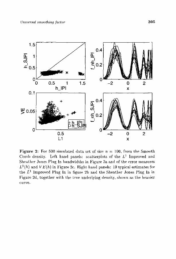
Universal smoothing factor 305
1.5
a. 1 - - j
cO 1 0.5
0
0.1
0 0.5 1 1.5 h_lPI
uJ > O.O5
0
~ + ~ -
0.5 L1
_ 0 . 4
I r
~10.2
0 -2 0 2
x
�9 . 0"4 I 0.2
....I
0 -2 0 2
x
F i g u r e 2: For 500 simulated data set of size n = 100, from the Smooth Comb density. Left hand panels: scatterplots of the L 1 Improved and Sheather Jones Plug In bandwidths in Figure 2a and of the error measures L 1 (h) and VE(h) in Figure 2c. Right hand panels: 10 typical estimates for the L 1 Improved Plug In in figure 2b and the Sheather Jones Plug In in Figure 2d, together with the true underlying density, shown as the heavier curve.

306 L. Devroye
respect to V E mostly by avoiding the proportion of quite large values that the L 1 Plug In suffers. On the other hand the L 1 Improved Plug In is bet ter in the L 1 sense, because the L 1 error is often slightly smaller. Note that most of the time each method is quite acceptable with respect to both measures.
An important way of comparing the performance of different bandwidth selection methods is to look at the resulting density estimates, as done in the right hand panels, Figures 2b and 2d. Again personal opinions will vary, but I much prefer the Sheather Jones in this case, because I am most interested in finding features such as bumps, and prefer not to see "bumps that are not really there". The L 1 Improved Plug In has too many spurious bumps in the region of the first large peak, although there is improved performance in other regions. This density would be most effectively est imated by a location varying bandwidth, which is large on the left hand side, and smaller on the right, but it is still interesting to see how well a constant bandwidth method can perform, especially as location varying bandwidths are not so well understood yet.
2.6 F i n a l r e m a r k s
It has been fun both reading this deep and informative paper, and also writing up this discussion. I am sure the author 's response will also be interesting. Again, I would like to stress the point from Section 1 above, that I view all of these "modern" bandwidth selectors as being effective da ta analysis tools.
R e f e r e n c e s
Fan, J. and J.S. Marron (1994). Fast implementations of nonparametric curve estimators. Journal of Computational and Graphical Statistics, 3, 35-56.
Farmen, M. (1997). An assessment of finite sample performance of adaptive meth- ods in density estimation. Unpublished manuscript.
Jones, M.C., J.S. Marron and S.J. Sheather (1996). A brief survey of bandwidth selection for density estimation. Journal of the American Statistical Associa- tion, 91,401-407.
Lindeberg, T. (1994). Scale-space theowin computer vision, Kluwer, Boston.

Universal smoothing factor 307
Marron, J.S. (1997). Assessing bandwidth selectors with visual error criteria, to appear in Computational Statistics.
Marron, J.S. and A.B. Tsybakov (1995). Visual error criteria for qualitative smoothing, Journal of the American Statistical Association, 90,499-507.
Sain, S.R. and D.W. Scott (1996). Zero-bias locally adaptive density estimators. Technical Report, Rice University, Available at: ftp.stat.rice.edu.
Schmitz, H.P. and J.S. Marron (1992). Simultaneous estimation of several size distributions of income. Econometric Theory, 8,476-488.
Silverman, B. W. (1986). Density estimation for statistics and data analysis, Chapman and Hall, London.
Wand, M. P., J.S. Marron and D. Ruppert (1991). Transformations in density estimation. Journal of the American Statistical Association, 86,343-361 (with discussion).
Yang, L. (1997). Root n convergent transformation kernel density estimation. Un- published manuscript, available at: http://www.wiwi.hu-berlin.de/pub/papers/ sfb373/sfb 1997/dpsfb970006.ps.Z.
Yang, L. and J.S. Marron (1997). Iterated transformation kernel density estima- tion. To appear in Journal of the American Statistical Association. Available at: http: / /www.wiwi.hu-berlin.de/pub /papers/sfb373 /sfb1996 / dpsfb960094.ps.Z.
C. SAnchez-Sellero Universidad de Santiago de Compostela, Spain
J. de Ufia Universidad de Vigo, Spain
This paper provides a review of the new methodology developed by Luc Devroye and Gabor Lugosi for smoothing factor selection and a compari- son with some of its best competitors. We would like to congratulate the author for the comprehensive s tudy accomplished here and for the graphi- cal presentation of the simulation results. We also admire the introduction of the minimum distance principle in the problem of density estimation and the appeal of establishing a relationship with the empirical measure. With respect to the theoretical results, we emphasize their application to all densities in all dimensions and their nonasymptotic character.

308 L. Devroye
The author has developed this methodology in two steps, published in two different papers, and here defined as "first and second bandwidths". In this paper an implementation of the first bandwidth is provided, but not of the second one. We wonder whether the first bandwidth could in fact be considered as an implementation of the second one.
We would like to raise two points regarding the application of the method. First, the parameter bn, that is, the upper bound of the can- didate bandwidths is assumed to go to infinity in Theorem 1. We think that it is enough to require the convergence to a constant. In fact, this upper bound is taken as the interquartile distance in the implementation. Second, the possibility of nonuniqueness of the minimum is pointed out. We feel this as a drawback of the method. How often does this happen?
In the practical implementation of the double kernel method, the author proposes four rescaling values for the second kernel L and asserts: "The theory tells us that for large n, the scale factor of L should exceed that of K" . This is nothing but a second bandwidth for the second kernel. We think that double kernel requires double bandwidth and we think that the author is of the same opinion.
According to the simulation study, the Ll-plug-in improved selector seems to be the best one. The new methods, at the bo t tom of the figures, have an overall good performance. However, we are worried about their problems with the simpler densities, most of them at the left side of the figures. We also observe in the simulation results that the iteration and rotation do not supply significant improvements to the Devroye-Lugosi se- lector. Given the increase in the computat ional cost that these procedures imply, we are not sure about their usefulness.
This methodology can and should be adapted to obtain two main pur- poses: To take advantage of some known properties of the da ta (for in- stance, knowledge of the support) , and to deal with special types of data. Regarding this lat ter case we have in mind the many types of incomplete data. In particular, we have designed a new bandwidth selector for random right censored data. This was done defining the total variation in this way:
^
where fn-m,h is the convolution of the rescaled kernel with the product- limit est imate under random censorship constructed with the first n - m

Universal smoothing factor 309
data points, and F,~ is the product-limit estimate with the test set of m data points. We stress the fact that suitable estimators of the distribution function could substitute the empirical estimate in order to obtain selec- tors adapted to many other contexts. In this sense, still under the model of random censorship, if we want to take advantage of the hypothesis of pro- portional censorship (submodel of the previous one), we could replace the product-limit estimator by the ACL estimator of the distribution function.
We carried out a small simulation study to assess the behavior of this selector and to compare it with a plug-in selector. We have chosen the plug-in selector adapted to censorship by Ss Sellero, Gonzs Man- teiga and Cao (1997). Weibull distributions with scale parameter 1 and shape parameters 1, 2 and 3 were chosen for the variable of interest and a proportional censoring model was simulated with a probability of cen- soring of 25%. One thousand samples of size 100 were generated. The numbers represent the averages over the one thousand samples of the ISE and the IAE (the values were multiplied by 1000 for ease of presentation). We can observe that the Devroye-Lugosi bandwidth adapted to censoring is perfectly competitive. We also point out that the introduction of the proportional censoring information gives place to an improvement in the performance. This was expected. Finally, in our experience we noted that the kernel density estimate with DL bandwidth has a better performance when it is constructed with the whole sample than when it is computed using only the first n - m data points.
Means of the ISE Means of the IAE Selector W(1, 1) W(2, 1) W(3, 1) W(1, 1) W(2, 1) W(3, 1)
DL with PLE 39.6 20.0 10.6 189 113 74.9 DL with ACL 34.3 16.9 8.98 176 103 68.6
Plug-in 44.1 21.0 8.85 181 109 65.3
Table 1: Results of the simulation study.
R e f e r e n c e s
Ss C., W. Gonzs and R. Cao (1997). Bandwidth selec- tion in density estimation with truncated and censored data. Preprint.

310 L. Devroye
F. U d i n a Univers~tat Pompeu Fabra, Spain
1 I n t r o d u c t i o n
I would like first to thank the editors for setting up this forum around the very interesting paper written by Luc Devroye and giving myself the opportunity to participate in it.
As I knew about the new methodology for bandwidth selection devel- oped by Devroye and Lugosi (DL), I was attracted by both the elegance and simplicity of the involved ideas and, of course, by the universality they achieve. My second thought was about the practical performance of these selectors. Luc Devroye has made a really great work by comparing the new methods with the classical ones and showing that they are very competi- tive. It would be very interesting to extend it to include sample sizes other than N -- 100.
In the following lines I want to discuss how Devroye-Lugosi bandwidth selectors behave in practice when facing real data sets. This concern two main issues: how to adapt the method to work in a binned data com- putational setting and how to protect the method against typical data manipulation such as rounding or sorting.
2 B i n n e d v e r s i o n of D e v r o y e - L u g o s i s e l e c t o r
Using kernel estimation techniques in practice means to use some discretiza- tion technique like binning as described, for example, in Fan and Mar- ron (1993) or, under the name of warping in Hgrdle and Scott (1992). It is the only practical way to deal with big or moderately big data sizes. For a given grid gk, {J = 1 . . .G) , bin counts ck are computed for the first n - m data points using linear binning. Then approximated estimates for density values are computed for every gk needing only a few kernel function values. The finite convolution needed can be computed even faster using fast Fourier transform techniques. We use in this quick study the global version of the "First bandwidth" as described in Devroye's paper. The slight changes we make to the algorithm will be commented. In this binned context, the approximated Yatracos set Aij is simply a union of bins (the

Unwersal smoothing factor 311
ones where fh, (gk) > f% (gk)) that can be coded as a bit vector of length G. Yatracos distance computat ion is really fast and simple in this situation.
A potential problem that would need some study appear: 'al though binning gives very good approximated density values we have no guarantee of having good approximation to the true Yatracos sets (whatever this means) and this can distort the distances to be minimized. Our experience show that the choice of G and the binning width w do not affect the selected bandwidth, provided that G is big enough and the width is small. We usually take G in the hundreds. Once w is fixed, we use it to decide the minimum bandwidth to be considered, because it makes no sense to take bandwidth values that would include less than several grid values in the computat ion.
3 D e a l i n g w i t h real d a t a s e t s
When we deal with real da ta sets we must be careful about how da ta has been transferred to the analyst. It's quite usual, for example, that da ta have been collected in rounded form or have been rounded a posteriori. Some bandwidth selectors are robust against any small change in da ta values, but the Devroye-Lugosi universal selector can have problems with repeated values. We will discuss some examples below.
Another source of problems can come from data being arranged in some way before arriving to the algorithm. Some of my time was spent inves- tigating strange behavior in the algorithms proposed by the paper. The reason was tha t the da ta were sorted in increasing order in the file where it came to me. Obviously the method doesn' t work at all with sorted data if split is done in the usual way, taking the first m values. Similar problems can appear if da ta are collected or t ransmit ted in a non-random ordering, by different categories, for example. Even in some Monte-Carlo simulations I found tha t some of my algorithms were generating da ta from normal mix- tures in a component-by-component way. This normally doesn' t have any consequence but when splitting the da ta set to apply the Devroye-Lugosi procedures, problems arose.
The strategy to follow when data is suspected to have been sorted is not easy to devise. One possibility is to shuffle randomly the da ta set and then to take the first m da ta values to build the empirical measure. This

312 L. Devroye
has the problem of producing a different selected bandwidth every time the algorithm is applied. As we will see in the examples, changing the m length subsample introduces a lot of variability in the selected bandwidth. In the paper, Devroyein t roduces the rotation idea to compensate it. The obvious drawback is that computat ion time grows, as the method itself is quite time consuming. Another possibility could be extracting the m da ta points in some systematic way. For example, a simple scheme could be, to take m elements out of n, sort the da ta set and take those with ordered index [ni/m] for i = 1 . . . m. But this needs some theoretical justification because violates the independence assumption and in case of repeated values would favor even more coincidences between the two subsamples.
4 S o m e r e a l d a t a s e t s
I was trying first to work with the Miguel Hidalgo s tamps da ta set brought to the density estimation area by lzenmann and Sommer (1988). It 's a da ta set that presents both a rich s tructure to s tudy and a reliable sample size (n---485). Da ta comes from thickness measured from a collection of old s tamps issued in 1872-74 in Mexico. But unfortunately, da ta is heavily rounded to thousandth of millimeters resulting in a high proportion of repeated data. This results in the impossibility to apply the described techniques to it. The Sheather-Jones plug-in bandwidth, for example, is 0.00272 for this da ta set, so it is in the same order of the resolution of the data. To select this bandwidth, DL would need to fix a minimum bandwidth so small that the estimates will result a series of single value peaks. When splitting the data, the m subsample results to be a subsample of the n - m one. The result is that the minimum bandwidth is selected most of the times the algorithm is run. Probably Devroye-Lugosi theory might be modified to work with smoothed discrete distributions and then some work could be done with this da ta set.
Postman, Huchra and Geller (1986) studied the velocities of 82 galaxies moving away form our galaxy. The da ta set was deeply analyzed from the kernel smoothing point of view in Park and Turlach (1992). They gave bandwidth values selected by several automatic selectors. Translated to our kernel, they found from 1.37 for least squares cross-validation to 3.48 for biased cross-validation. For the Sheather-Jones plug-in they gave 1.44 and 2.72 for the normal-reference rule-of-thumb. The da ta set arrived to

Universal smoothing factor 313
me sorted in increasing order, so the re-shuffling strategy was applied.
# of h values m/n 10 20 30 40 0.1 0.2 0.3 0.4 0.5
1.339 1.686 2.543 2.626 1.928 1.418 1.811 1.724 2.777 3.365 3.189 3.107 2.777 2.382 2.271 2.414 1.928 1.686 1.811 1.724
F i g u r e 1: Values selected by the DL algorithm as described in the text, for several values of m/n and of the number of estimators in contest.
Applying the version of DL selector described above we obtained values around 2.0, depending on parameter choice. To show how the value selected depends on these parameters, we shuffled the da ta set once (it arrived to me sorted in increasing order again) and we run the algorithm with 7n being 10%, 20%, 30%, 40%, and 50% of the da ta size n = 82 and taking the number of different values for h in the range [0.15, 4.0] as 10, 20, 30, and 40. The minimum bandwidth is fixed as 1.5 times the binning width (so ensuring that at least three bins are involved in any computat ion). The maximum bandwidth is chosen to be the interquartilic range. The resulting values are shown in the table in figure 1. The variability of the selected parameter is noticeable. As expected, higher values of the ratio m/n give less variability. But even using the same pair of parameters, shuffling da ta can give very different values for the selected bandwidth. For example, with m/n = .3 and 20 bandwidth values, we obtained 0.423, 1.418, 1.418, 1.686, and 1.193 in five runs of the algorithm with re shuffling. To test the rotation idea suggested by Devroye, we took m = n/2 and computed the geometric mean of the two selected bandwitdhs obtained using both halves alternately as m subsample. Number of bandwidths in contest were 20 in the range [0.15, 4.0]. The values obtained were 0.775, 1.004, 1.094, 1.546, 1.546. We see tha t variability has not improved so much. As a mat te r of curiosity, we also show in figure 2 the shape that Yatracos sets appear to have. For 10 bandwidth values (from .15 to 4.0 in geometric steps) we generated 10 density estimates f l , . . . , fl0 and computed the Yatracos sets Aij = {xlfi(x ) > fj(x)} Each horizontal line in figure 2 represent a set. The lower band composed by nine lines corresponds, as going up, to Alj, j = 2 , . . . , 10 and so the other 10 bands.

314 L. Devroye
~ ' i I - - - - - - ~ - - Z Z . . . .
. I _ . . . . . . . . . . . . . . . .
: : : : : : I : 2 : : : : : : : : : . . . .
i I - - ~ = i
- - - : : - - ' : 2 - - - - = " - - - - - _ - - - - - - - - : . . . . . . . . . . . . . . . . . . . . . . . .
_ - - - _ :~_~__--:'I: -
: : : : = = _ - : : : : : : : : : : - : : - : . - - : : - _ - : : :
: : _: : : y : : i . - : . . : : - : " Z
- - - - . : : . . ~ i : : . : ' Z - : I Z - Z " Z X Z Z Z - - i
: _ - - Z : Z Z : : --- : - - . Z Z--- Z Z Z Z Z
I I I I I
0 10 20 30 40
Figure 2: Yatracos sets for galaxies data
Most of the variability found in the selected bandwidths for the galaxies da ta can be explained by the sample size being too small. We decided to contrast it with the case of a very big da ta set, also well known in the smoothing literature. The net income of 7201 British households in the year 1975 was studied in Schmitz and Marron (1992) and also discussed in Wand, Marron and Ruppert (1991). Data range goes from 0.026 to 9.1225 the unit being the average income. Despite the da ta range and resolution, the set contains a quite high number of repeated values, namely 1357. We took a grid size of 800 in the range -1 to 10, so the minimum bandwidth to be considered is approx .022. The maximum was taken here as half the interquartilic range and 25 bandwidth values were taken in the resulting interval [.022, .4]. m was chosen to be 25% of the sample size. In figure 3 we plot Yatracos distance over (logarithm of) bandwidth values. 8 different runs are plotted resulting from re shuffling before split. The selected bandwidths were 0.051, 0.058 twice, 0.065 three times, 0.094 twice, 0.106 and 0.152. We see that variability is somewhat reduced but it's still quite high. Applying the systematic split discussed in section 2 selected a bandwidth of 0.025, clearly too small. The reason can be the relatively

Universal smoothing factor 315
high percentage of repeated values. Applying the rotation algorithm in this setting resulted to more reasonable and stable values, we got 0.10, 0.094, .081 in three different runs.
o o
r
o (5
t~
o
o
o d
- 3 , 8 1 7
Income 75 data
4' ~x
W I I ~ \A . 'I i x
i l 1 I
- 3 . 0 9 2 - - 2 . 3 6 7 - 1 . 6 4 1 - 0 . 9 1 6
F i g u r e 3: Values for the Yatracos distance in vertical axis. In horizontal axis, log of bandwidth. Each line is a diferent run of the algorithm with previous data shuffling.
5 C o n c l u s i o n
We have seen that to use the DL selectors with real data, binning techniques can be used but some problems must be faced. The main one is how to deal with repeated values - this seems to need some theoretical adjustment. The other problem is to protect the algorithm against data that can be sorted or arranged in some non-random way. It looks like the shuffling-then-rotate approach is the safer one but further study is needed.

316 L. Devroye
R e f e r e n c e s
Fan, J. and J.S. Marron (1992). Best possible constant for bandwidth selection. Annals of Statistics, 20, 2057-2070.
Hs W. K. and D.W. Scott (1992). Smoothing by Weighted Averaging of Rounded Points. Computational Statistics, 7, 97-128.
Izenman, A. J. and C. Sommer (1988). Philatelic Mixtures and Multimodal den- sities. Journal of the American Statistical Association, 83, 941-953.
Postman, M., J.P. Huehra and M.J. Geller (1986). Probes of large scale structures in the Corona Borealis region. The Astronomical Journal, 92, 1238-1247.
Park, B. U. and B.A. Turlach (1992). Practical Performance of Several Data driven bandwidth selectors. Computational Statistics, 7, 251-270.
Schmitz, H.P. and J.S. Marron (1989). Simultaneous estimation of several Size Distributions of Income. Discussion paper A-186, SFB 303, University of Bonn, Dept. of Economics.
Wand, M. P., J.S. Marron and D. Ruppert (1991). Transformations in Density Estimation. Journal of the American Statistical Association , 86,414,343-361.
Rejoinder by L. Devroye
Sometimes, researchers charge ahead like young bulls in a bullring, hit- ting anything tha t moves in the arena, but oblivious to the sword that will eventually kill them. That is exactly how I feel after reading some of the comments. If the newly proposed methods are to be used in practice, as Frederic Udina points out, more work is needed to address the problems of the selection of a random subset and of real da ta with repeated values. On his transparencies, Frederic used the phrase "repeated values kill Devroye- Lugosi ' . C~sar and Jacobo correctly point out tha t our work on the double kernel is unfinished: the unstudied double kernel/double h method is likely the one tha t will survive most matadorial attacks.
Many comments relate to generalizations of the new estimates or im- provements of the kernel estimate. These include transformed kernel esti- mates (Steve and Jan), locally adaptive estimates (Steve again), support-

Universal smoothing factor 317
sensitive estimates (C~sar and Jacobo), symmetry-sensitive estimates (Ri- cardo Cao), generalizations to censoring (C~sar and Jacobo), and param- eter selection in nearest neighbor estimates (Ricardo Fraiman)., All these comments are pertinent and show real concern regarding the kernel esti- mate's performance. We are pleased that our study has uncovered new problems related to kernel density estimates. The existence of just a few patterns of behavior across the spectrum of densities (figures 6 through 10) prompted Peter Hall to suggest the automatic selection of a bandwidth selector based upon entropy estimates. This could also be done based on spacings. Indeed, if we had a further i.i.d, sample Z 1 , . . . , Zk with order s t a t i s t i c s Z(1 ) < . . . < Z(k), then fzZ~_l f,,, 1 < i < k + 1, with Z(0) = - o c and Z(k+D = oc should ideally be distributed as uniform spacings. A stan- dard spacings test may be used to identify the best bandwidth selector. A related method was included in the simulations of Berlinet and Devroye (1994) to select the best h in the kernel method, but it yielded mediocre results. Nevertheless, this avenue of research should prove useful.
No simulation study can ever be conclusive. Both Chris Jones and Steve Marron point out some problems with the selection of our test densities and with the interpretation of the results. For example, it is clear that all bandwidths that optimize some criterion perform rather abysmally on near-normal densities relative to plug-in methods. To expose behavior of this sort was precisely one of our goals. One should not forget that we set out to develop bandwidths with new broad performance guarantees, and that the simulation study came later. The instability of the Ll-improved plug-in method discovered by Steve is indeed puzzling. To make matters worse, the second bandwidth of Devroye and Lugosi (1997) is simply un- implementable as it involves minimization of a function over an infinite space, and each function value requires a supremum over an uncountably infinite ensemble. At this stage, we should take the bull by the horns and place the selectors in the hands of agile bandwidth engineers to fine-tune, adjust, modify, robustize and tame.
Chris Jones mentions that we should have used a fuller version of the Sheather-Jones bandwidth. We picked the one used in the study by Cao, Cuevas and Gonzs (1994), in part to have a standard of com- parison with that study. In his comment, Steve Matron confirms our sim- ulation results with respect to the Sheather-Jones bandwidth, but it was not clear which version Steve used.

318 L. Devroye
Chris Jones and to some extent Steve Marron wave the red banner for the choice of the Bartlett-Epanechnikov kernel in the simulation study. There were various reasons for our decision. Among positive kernels, it is optimal for L1 and L 2. It is computationally convenient as the kernel est imate is piecewise parabolic. We also suspect that the relative perfor- mance of various bandwidth selectors will not change much among smooth unimodal positive kernels. However, more importantly, one might consider the joint data-based choice of K and h. This should improve the absolute performance, but perhaps not for small sample sizes. If the complexity of the family of kernels K can be controlled (in the computat ion of the Vapnik-Chervonenkis shat ter coefficient), then methods similar to those of Devroye and Lugosi (1997) may be useful. Gs comments in fact read as a mini-paper in which he shows the way for parametr ic families of ker- nels. We thank him in particular for working out a d-dimensional example in which the kernel est imate has d scale parameters.
Steve sticks his banderilla in the right spot when he remarks that n -- 100 is too small for some densities in our study. But that is precisely our point too. Those are the densities that can be classified as difficult. Thus, our simulation study covers many different virtual (or relative) sample sizes. We can get more information either by changing n or by adding more densities and keeping n fixed. Eventually, if we increase n, all densities will appear easy, so increasing n alone will not be sufficient in a study.
The choice of the L1 criterion is based on arguments related to the estimation of probabilities, generating new approximate samples from the unknown density, invariance under monotone transformations, visual dis- tance between curves, and the universality of the error scale. Our band- widths are designed with the L1 criterion in mind. Matron and Tsybakov's VE is different and requires appropriate and new bandwidth selectors. We unfairly threw sand in the readers' eyes by comparing the Sheather-Jones bandwidth with the Ll-improved plug-in method (as the former was de- signed for L2). In the same vain, one should not compare our bandwidths with other ones based on VE, for example. It is also unclear whether in his comparison, Steve used VE(1), an L1 version of VE, or VE(2), which by definition should favor L2 bandwidth selectors such as Sheather-Jones. If f is Lipschitz, then VE(1) (f~ --~ f ) divided by f Ifn - f] is always be- tween 1 /v / i -+ C 2 and 1~ so tha t we suspect VE(2) was used. Much blood can be spilled over the question of why we do density estimation. Chris Jones points out that if we are interested in probabilities, we should stick

Umversal smoothing factor 319
to empirical distribution functions. These are only good for probabilities of intervals, not probabilities of Borel sets. Indeed, the finite set of the data receives mass one from the empirical distribution function but has in fact zero probability whenever a density exists. Density estimates with good L1 properties provide good probability estimates uniformly over all (possibly data-dependent!) sets.
The paper builds on experiments first reported by Berlinet and De- vroye (1994) and on theoretical results with Gs Lugosi (1996, 1997). Alain's cooperation during the last few years is gratefully acknowledged, while Gs should have been a coauthor of the present paper (l asked him but he refused to enter the ring). Various commenters refer to equa- tion (7), which was changed to (8.7) in the final printed version. We also corrected typographical errors reported by C@sar and Jacobo. We changed only one sentence in the original manuscript after a comment by Steve that (8.1) is not always close to the optimum, as we hastily and incorrectly claimed. We thank Domingo Morales for a thorough job as editor and we thank Test for allowing us to publish five color figures. Finally, we thank Antonio Cuevas and Wenceslao Gonzs for the warm reception in Santiago, where we read our paper on September 11, 1997, and hit all moving objects thrown at us by Ricardo Cao, Frederic Udina and C~sar Sanchez-Sellero. They stopped just short of singing the Malaguefia.
Let me conclude with a few open problems of my own. These show a strong personal bias and may be the last nervous jerks of an impetuous but wounded bull.
. (1) Establish if the class of asymptotically optimal bandwidths is empty. Can the 3 in the bounds be replaced by 1 for some bandwidth selector?
. (2) If the answer to (1) is negative, one should develop asymptotically optimal bandwidths for all densities in certain subclasses. We do not know for example how to pick an asymptotically optimal bandwidth for all monotone densities on the positive halfline. As there are in- finitely many classes of densities, this is like letting the prize bull loose in the cow barn.
3. (3) Is the double kernel bandwidth suitable?

320 L. Devroye
4. (4) Study the double kernel/double h method. Is it universally suit- able?
5. (5) Study the properties of the iterative method of section '6.
6. (6) Study the sensitivity with respect to changes in subsets of the data of size k. That means studying the supremum of the L1 error after the supremum is taken over all subsets of k out of n and all values on the real line for the k selected data points.