1196432:

UNIUERSITV DF SURREY LIBRRRY

ProQuest Number: All rights reserved

INFORMATION TO ALL USERS The quality of this reproduction is dependent upon the quality of the copy submitted.

In the unlikely event that the author did not send a com plete manuscript and there are missing pages, these will be noted. Also, if material had to be removed,

a note will indicate the deletion.

uestProQuest 10130240

Published by ProQuest LLO (2017). Copyright of the Dissertation is held by the Author.

All rights reserved.This work is protected against unauthorized copying under Title 17, United States C ode

Microform Edition © ProQuest LLO.

ProQuest LLO.789 East Eisenhower Parkway

P.Q. Box 1346 Ann Arbor, Ml 4 81 06 - 1346

A RADIO WAVE PROPAGATION STUDY USING THE OLYMPUS BEACON Bi

BilaS Ahmed Centre for Satellite Engineering Research

University of Surrey

Thesis submitted to the University of Surrey for the Degree of Master of Philosophy

April 1993

In the name o f God? Most Gracious, Most Merciful

I1. Proclaim ! In the name of your Lord and Cherisher Who created

2. Created man, out of a mere clot of § LlX l* J 1 icongealed blood: y

3. Proclaim ! And your Lord is Most Bountiful,-

4. He Who taught the use of the Pen,-

5. Taught man that which he knew not.

00 hU Jk__V

Allah the Greatest Says the Truth

Dedicated to the Unique Creator for His unique creation "The Universe"

ABSTRACTRapidly growing demand for channel capacity and limitations in satellite power and frequency spectrum is urging the utilisation of higher frequency bands. Attentions are focused on 20/30 GHz and above which will provide many services due to large the available bandwidth and small size of earth segment. However, the main problem revolves around the severe attenuation by hydrometeors, specifically rain which significantly degrades communications quality.

The available propagation data in 20/30 GHz bands in Europe is not sufficient for designing reliable communication systems. Olympus provides a unique opportunity for collection of long term propagation data to investigate the effects of hydrometeors at12.5, 20 and 30 GHz. An experimental arrangement has been established for 20 GHz beacon measurements at the University of Surrey. Copolar and cross polar measurements were taken but only the copolar attenuation data has been analysed.

On 29th May 1991 Olympus lost attitude and orbit control. In its absence the Russian satellite (MAYAK) transmission was recorded, after modification in the receiving equipment. Data recorded from the MAYAK beacon had large cyclic variation, a peak to peak variation of several decibels was observed which were removed at the data pre­processing stage. A limited data was collected from MAYAK since Olympus was restored in mid August 1991 and beacon measurements were continued as before. A few significant propagation events recorded using MAYAK are also presented in the thesis. Olympus showed peak to peak diurnal variation of few decibels which was removed by the data pre-processing software before any statistical analysis of the data.

Another experimental arrangement for collection of weather data has also been established. A new time integration technique for calculation of rain rate using low resolution rain gauge has been introduced which produced better results and they were verified using rain attenuation prediction models.

The limited data set obtained from Olympus and MAYAK beacons was compared with rain attenuation models as well as European and UK experimental results. Cranes rain attenuation prediction for Guilford yielded best fit to the measured data. There is also a good correlation with the other European measurements. However, comparison with the

BTRL was not in full agreement because the BTRL measurements were taken uninterruptedly over a period of one year while the measurements taken at Guildford were short term and interrupted several times due to loss of Olympus, software and hardware development for alternative satellite. Long term data is required for more meaningful comparison. The system has been developed to receive and record data reliably. Data recording is in continuous progress more than one year's data has been obtained but only preliminary recorded data is analysed in this thesis.

LIST OF CONTENTS

ABSTRACT ............................... (i)

LIST OF CONTENTS .................... . (iii)

ACKNOWLEDGEMENT .......... ..... (vSi)

ABBREVIATIONS ................ ............ (viii)

CHAPTER 1INTRODUCTION

1.1. DEVELOPMENT IN SATELLITE COMMUNICATION ...... (1)1.2. PROBLEMS WITH THE AVAILABLE FREQUENCY BANDS . (2)1.3. SATELLITE BEACONS ABOVE 10 GHz ................ (3)1.4. 20/30 GHz MEASURMENTS ................ (9)1.5. UTILISATION OF OLYMPUS BEACON PACKAGE ...... (10)1.6. AIM OF RESEARCH .......................... (11)1.7. OUTLINE OF THE THESIS .......................... (11)

CHAPTER 2RADIO WAVE PROPAGATION THROUGH THE TROPOSPHERE

2.1. TYPES AND FEATURES OF RAINFALL ............... (12)2.1.1. Stratiform Rain (12)2.1.2. Convective Rain (13)2.1.3. Spatial Distribution Of Rain ..................... (13)2.1.4. Measurement Of Rain Cell Extent ................ (13)

2.2. TROPOSPHERIC ATTENUATION ..................... (13)2.2.1. Rain Attenuation (14)2.2.2. Gaseous Attenuation (16)2.2.3. Hydrometeor Attenuation ..................... (19)2.2.4. Attenuation Due To Other Factors ................ (20)

2.3. SCINTILLATION (20)2.3.1. Ionospheric Scintillations ..................... (21)2.3.2. Tropospheric Scintillations ..................... (21)2.3.3. Wet And Dry Scintillations ..................... (23)2.3.4. Tropospheric Scintillations Characteristics ........... (24)

2.4. DEPOLARISATION (25)2.4.1. Rain Depolarisation .......................... (26)2.4.2. Ice Depolarisation .......................... (26)

2.5. RADIO NOISE (26)2.5.1. Solar Noise ............................... (27)2.5.2. Atmospheric Gaseous Noise ..................... (27)2.5.3. Hydrometeor Noise (27)

CHAPTER 3RAIN ATTENUATION PREDICTION MODELS

3.1. CCIR RAIN ATTENUATION MODEL ................ (35)

3.2. CRANE RAIN ATTENUATION MODEL ................ (41)

3.3. THE SIMPLE ATTENUATION MODEL ................ (44)

3.4. LIN RAIN ATTENUATION MODEL (46)

iv

3.5. COMPARATIVE EVALUATION OF MODELS (48)

CHAPTER 4MODIFICATION IN THE EXPERIMENTAL ARRANGEMENT FOR Ka BAND MEASUREMENTS4.1. OLYMPUS BEACON PAYLOAD ..................... (64)

4.2. OLYMPUS LINK BUDGET (64)

4.3. SYSTEM CONFIGURATION FOR B j MEASUREMENTS ...... (66)4.3.1. Development Of The Down Converter ........... (67)

4.3.1.1. Filters and test performances ........... (68)4.3.1.2. Amplifiers and test performances ........... (69)4.3.1.3. Mixer and oscillator (70)

4.3.2. Down Converter As A Subsystem (70)

4.4. BEACON RECEIVER AND TEST PERFORMANCE ...... (71)

4.5. WEATHER STATION (74)4.5.1. Data Logging And Display ..................... (75)4.5.2. An Adaptive Time Based Technique to Determine Rain Rate (76)

4.6. LOSS AND RECOVERY OF OLYMPUS (77)

4.7. MAYAIC AS AN ALTERNATIVE SATELLITE ........... (79)

CHAPTER 5RESULTS OF MEASUREMENTS TAKEN USING ka BAND BEACONS5.1. OLYMPUS B j DATA COLLECTION.................... (91)

V

5.2. B i DATA PRE-PROCESSING.......................... (92)

5.3. B i DATA PRESENTATION .......................... (93)

5.4. B i DATA ANALYSIS .......................... (94)5.4.1. Fade Duration (95)5.4.2. Rate Of Change Of Attenuation ................ (96)

5.5. PERCENT OF TIME PERFORMANCE ................ (97)

5.6. EXPERIMENTAL RESULTS AND DISCUSSION ........... (98)

CHAPTER 6CONCLUSION AND FUTURE W O R K ........... (136)

REFERENCES .. ..... (140)A PPEN D IX IBAND PASS FILTER (147)

A PPEND IX IIPCW INTERFACING CARD ........... (149)

A PPEND IX IIINPCW DATA ACQUISITION .......................... (151)

APPEND IX IVDATA PRE-PROCESSING AND ANALYSIS PROGRAMMES ..... (157)

A PPEND IX VPUBLICATIONS (166)

vi

ACKNOWLEDGEMENTI would like to sincerely thank Almighty God (Allah). Who taught us with pen and through other means. Who kept me physically fit all the way through this course. Who gave me strength to face difficulties appeared from time to time during the experimental measurement and writing up of this thesis and otherwise. Who gave me caring and loving parents and a very understanding wife. (Then which of the favours Of your Lord will you deny; Al Qur'an, chapter 55: Rahmaan).I would like to thank Professor B. G. Evans and Dr. M. S. Mahmoud for accepting me as a research student and the guidance which they offered me when ever required.My best regards and thanks to my elder brothers Z. Ahmed, F. Ahmed, I. Ahmed and sisters for their financial support. I received a lot of moral support from my parents and in laws and friends such as K. Hafeez, R. M. Suddle, S. M. Athar, G. Butt and J. Ahmed, thanks to all of them.During the course I learned a lot and missed a lot. Finally my all thanks to Allah for His bounties and blessings.

vii

ABBREVIATIONS

ACTS Advanced Communication Technology SatelliteAve AverageApprox ApproximatelyArtemis Advanced rely and technology missionASCII American Standard Code for Information InterchangeATS Application Technology SatelliteAT&T American Telephone and TelegraphAug AugustBPF Band Pass FilterBSE Broadcasting Satellite ExperimentBTRL British Telecommunication Research LaboratoryB W BandwidthCCIR International Radio Consultive CommitteCODE CO-operative Data Experimentcs Communication SatelliteCTS Communication Technology SatelliteCW Contineous WaveDAPPER Data Analysis and Pre-Processing Effects ResearchdB DecibelDBR Digital Beacon ReceiverDFS Deutsche Fernmelde Satellitedia DiameterE EastEIRP Equivalent Isotropically Radiated PowerESA European Space AgencyETS Engineering Test SatelliteFig FigureFreq FrequencyGHz Geiga Hertz (10 Hertz)gm Gramshex HexadecimalHHI Horizontally transmitted Horizontally received In phaseHHQ Horizontally transmitted Horizontally received Quadrature phase

hrs HoursH-Sat Heavy Telecommunication SatelliteIF Intermediate FrequencyIL Insertion Lossrr Integration TimeK KelvinKHz Kilo Hertz (103 Hertz)Km Kilo meter (103 meters)LNA Low Noise AmplifierLO Local OscillatorLPF Low Pass FilterL-Sat Large telecommunication SatelliteMHz Mega Hertz (10 Hertz)min Minutem m Millimetremm/hr Millimetre per hourM P C W Modified Personal Computer WeatherN NorthNASA National Aeronautics and Space AdministrationOct OctoberOPEX Olympus Propagation ExperimentOTS Orbit Test SatellitePC Personal ComputerPCW Personal Computer WeatherPLL Phase Lock LoopPPM Parts Per MillionRAM Read Access MemoryRep ReportRF Radio FrequencyS SouthSAM Simple Attenuation ModelSec SecondSep SeptemberTemp TemperatureUHF Ultra High FrequencyUK United Kingdom

USA United States of AmericaUTC Coordinated Universal TimeUnlv UniversalVHF Very High FrequencyVHI Vertically transmitted Horizontally received In phaseVHQ Vertically transmitted Horizontally received Quadrature phaseW West

X

CHAPTER 1

INTRODUCTION

Artificial satellites which man first constructed in the later half of this century have been able to play a significant role in the peaceful social development of mankind. Earth orbiting satellites are employed extensively for the relay of information in a vast array of telecommunications, meteorological and scientific applications. These satellite systems rely on the transmission of radio waves to and from the satellite, which is dependent on the propagation characteristics of the medium. Radio wave propagation thus plays an important part in the design and ultimate performance of satellite communication systems.

This chapter describes briefly the early developments of satellite communication. Also discussed is the need for characterisation of radio wave propagation medium at 20 GHz, which is the aim of this study work. An outline of the thesis will also be given.

l . L D E V E L O P M E N T IN S A T E L L IT E C O M M U N IC A T IO N

The moon as a passive reflector has been used by the US Navy in the 1950s for a low data rate communications link between Washington DC and Hawaii [Pratt, 1986]. This can be regarded as the first operational communication satellite link, In 1957 the Soviet satellite Sputnik-1 was launched. Since then numerous results have been achieved in space exploration, communication, meteorology, and geodesy.

The National Aeronautics and Space Administration (NASA) launched the first meteorological satellite, Tairos I in a circular orbit of about 700Km altitude, with a 48.3° inclination and a 99.2 minute period in April 1960. This can be regarded as the first man made satellite communication experiment in the world in passive relaying where no amplifier was used on board the satellite.

The American Telephone and Telegraph company (AT&T) launched Telstar I satellite in July 1962, and NASA launched Relay I satellite in December 1962. These satellites had disadvantages such as the short communication periods due to low altitude and the tendency of shifting in accordance with their apogee period. The possibility of global satellite communications was enhanced after the successful launching of Syncom II, the

l

first geostationary satellite by NASA in July 1963. In August 1964 another satellite, Syncom III, was launched and utilised for television transmission of the Tokyo Olympic Games [Miya, 1985]. A remarkable result was achieved in satellite communications nearly 20 years after A. C. Clark [Clark, 1945] suggested three geostationary satellites in the three ocean region for global coverage.

The communication via satellites and its applications in other fields progressed in the intervening period. The success of satellites created more demands for communications with the inevitable trend of moving towards higher operating frequencies. A series of experimental satellites opened the way for later operational satellites and demonstrated the new technology in space.

1.2. PROBLEM S W IT H TH E A V A ILA B L E FR EQ U EN C Y BANDS

Atmospheric effects on earth-space links are of prime concern in the design and performance of satellite communication links. The problems become more acute for systems operating in the frequency bands above 10 GHz. Satellite communication links operating above 10 GHz can be adversely affected by precipitation, atmospheric gases, clouds and fog. These conditions, when present alone or in combination on the radio wave link, can degrade the link quality and result in outage.

The major drivers in the development of satellite communications, which have increased the need for a further awareness and understanding of the propagation factors are:

© Rapid utilisation of frequency spectrum below 20 GHz .© Increasing demand for more bandwidth.© Limited number of orbital slots.(a). Rapid utilisation of frequency spectrum below 20 GHzSatellite communication services providers traditionally operating below 10 GHz have had to move to higher allocated frequency bands because of the lack of frequency allocations.

2

(b). Increasing demand for more bandwidthSatellite communications applications are requiring larger information rates to meet the needs of expanding telecommunications services. The frequency bands above 10 GHz have much larger bandwidth allocations.(c). Limited number of orbital slotsSpacing requirements for satellites operating in the same frequency band impose upper limits on the number of satellites that can occupy geostationary arc. Presently there are more than two hundred satellites in the geostationary orbit operating at different frequencies which is a clear sign of orbital slots limitation. Table (1.2.1) gives the total number of geosynchronous satellites currently in operation and will be operational at different frequency bands in future [Rees, 1990; Chetty, 1991 and Martin, 1991].

Table(1.2.1)Total number of satellites in operation and will be operational in future.

Presently in operation Planned for futureI Frequency bands Frequency bands

L C ku ka L C ku ka14 109 89 14 11 89 120 4

1.3. S A T E L L IT E BEACONS ABOVE 10 GHz

In this section an overview of satellites offering beacon measurements above 10 GHz in the past is described, also discussed the present and future possibilities of propagation measurements using geosynchronous satellites.

Atmospheric effects in the 4 to 8 GHz bands are relatively mild. Measurements in this frequency range have been accomplished using the regular equipment on communication satellites. The need for more bandwidth is causing systems to be designed using allocated bands above 10 GHz. Above this frequency, both atmospheric gases and rain can have significant effects on communication links. Many experiments are being conducted, particularly to quantify the attenuation and polarisation effects of rain in the 10 to 30

3

GHz range of frequencies. Table (1.3.1) gives details of the main satellites which have been used for beacon measurements above 10 GHz.

Table(1.3.1).Satellites used for radio wave propagation measurements above 10 GHz

Satellite Beacon (s) GHz

Initialorbitallocation

Launchingdate

DesignLife

Stationkeeping

ATS-5 15.3 70° W 12.08.1969 3 yearsATS-6 20, 30 940 W 30.05.1974 2 years -CTS 11.7 116° W 17.01.1976 2 years ±0.2 E/W

COMSTAR 19.04, 28.5 76°W 22.06.1976 7 years ± 0.1 N/S and E/W

ETS-II 11.5, 34.5 130° E 23.02.1977 2 years ± 0.5 E/W! SIRIO 11.6 15° W 25.08.1977 2 years _

CS 19.45 136° E 15.12.1977 3 years ±0.1 E/W and N/S

BSE 12 110° E 07.04.1978 3 years ± 0.1° E/W and N/S

OTS 11 10° E 11.05.1978 3 years ± 0.1° E/W and N/S

First generation NASA Application Technology Satellite (ATS) evolved from the Syncom study. ATS-5 was the first satellite to have equipment for propagation measurements above 10 GHz, experiments were designed to measure atmospheric effects in radio wave propagation. ATS-5 was successfully placed into synchronous orbit. The satellite was to be spinning upon injection and then despun. During orbital injection the satellite developed a spin about an axis normal to the intended spin axis. In this orientation, the satellite could not be despun. Because of the spinning condition the satellite antennas pointed toward the earth only a small portion of revolution. Hence, the experiments were operated with limited success in a pulse type of operation synchronised with the periods of correct antenna orientation.

4

ATS-6 satellite was the second generation of the NASA's ATS program. Experiments on ATS-6 were for communications and propagation that covered a frequency range from 860 MHz to 30 GHz. ATS-6 was launched in May 1974. It was originally positioned at 94° W longitude. During June 1975, it was moved to 35°E longitude for the instructional television experiment broadcasts to India. At the same time, the NASA millimetre wave experiment was used in conjunction with several European ground terminals [ATS-6, 1977]. In the fall of 1976, the satellite was slowly returned to the Western hemisphere and located at 140° W longitude. It was turned off in the summer of 1979.

ATS-6 had two millimetre wave experiments. The NASA's propagation experiment used a C band uplink and 20 and 30 GHz down links, where as the communication satellite corporation propagation experiment used 13 and 18 GHz uplink and a C band down link [Hyde, 1975]. The continuous wave propagation tests had sufficient power to accommodate fades as deep as 60 dB.

CTS (communication technology satellite), formerly called Co-operative Application Satellite (CAS-C), was a joint effort of the Canadian department of communication and NASA. In May 1976, the CTS was renamed Hermes in Canada. It was used until November 1979. Beacon measurements at 12 GHz were taken and results have been described in [Ippolito, 1976].

The AT&T system started operating in 1976 using the COMSTAR satellites. COMSTAR was a dual spin type satellite. The communication subsystem and antennas were mounted on a despun shelf, which was oriented to keep the antennas earth pointing. In addition to the communication subsystem, all satellites had beacon transmitters for use in propagation measurements. Four satellites were launched, the orbital history of these satellites is as follows:

© Launched 13th May 1976, moved above synchronous orbit 1988.© Launched 22nd July 1976, 76° W longitude, spare, 6° inclination in 1991.© Launched 29th June 1978, turned off 1984 and moved above synchronous orbit.© Launched 21st February 1981, 76° W longitude, spare, 5° inclination in 1991.

Some results of COMSTAR beacon measurements have been documented in [Harris et al., 1977].

5

Japan's Engineering Test Satellite-II (ETS-II or Kilcu-II) was a beacon satellite whose objectives were to develop and test Japan's ability to launch and control a synchronous orbit satellite and to make propagation measurements. It was a spin stabilised satellite with a set of three antennas that were despun. Each antenna was used for one of the beacon transmission, which were at 1.7, 11.5 and 34.5 GHz. All three frequencies were derived by multiplication from a common oscillator at about 213 MHz. The propagation measurements in the ETS-II program were signal level and cross polarised level at each frequency and phase differences between several pairs of signals and cross polarised components. Some results have been documented in [Fugono et al., 1978 and 1980].

Italian industrial research satellite (SIRIO) was launched for use in propagation and communication experiments, 17.4 GHz frequency was the uplink while 11.6 GHz was the down link. Attenuation measurements were made on 11.6 GHz [Ramat, 1979]. Initially the SIRIO was positioned 15° W, later moved to 12° E longitude and in the first term of 1983 positioned at 65° E longitude and was in use until 1985.

Japan's Communication Satellite (CS) was used for a variety of tests and pre-operational system demonstration. Activities included transponder characterisation, tests of several transmission and multiple access techniques, gaining satellite control experience and propagation measurements. After launch the CS was renamed as Sakura which translates to cherry blossom. Sakura was moved above the synchronous orbit in early 1983.

Japan launched a medium scale Broadcasting Satellite for Experimental purpose (BSE) in April 1978. The BSE was three axis stabilised with deployed solar arrays. It was renamed Yuri (Lily) after launch. A series of experiments using this satellite was started in July 1978. Propagation measurements were carried out at 12 GHz on the down link [Fukuchi et al., 1983; Tsukamoto, 1978].

Orbit Test Satellite (OTS) was basically experimental in nature and had the following objectives:

© Demonstrate the performance and reliability of the satellite subsystem.© Demonstrate the proposed operational capabilities and provide the capacity for pre-

operational transmissions.© Gain experience in communication satellite system operation.© Perform propagation measurements at 11 and 14 GHz.

6

The satellite was three axis stabilised with two solar arrays that deployed after synchronous orbit had been achieved. The solar arrays rotated about their axis to track the sun. Initially OTS was placed in synchronous orbital position of 10° E longitude in 1978, moved to 5° E longitude in 1982 where it stayed until the end of 1983 later moved above the synchronous orbit. Some propagation measurements taken were analysed [Dintelmann, 1981].

European researchers had availed the limited opportunity of 20/30 GHz beacon measurements in the mid 70s when the ATS-6 satellite was moved to 35° E longitude for one year. Thirteen years later propagation measurements started again after launching ofthe Olympus satellite. Italsat and DFS-Kopernilcus are the other two satellites presentlyhaving beacon signals on board the satellites. The data collected from these three satellites by several experimenters in Europe will be useful for future communication systems designing in the ka frequency band.

The Olympus development began in 1982. Former program names include Large Telecommunication Satellite (L-Sat), Heavy Telecommunication Satellite (H-Sat) and Phebus. The objectives of the Olympus program are to:

© develop and demonstrate a large satellite platform© develop communications hardware and provide an orbital demonstration of new

communication services.© provide propagation measurements facility to meet future needs.

The European Space Agency (ESA) launched the Olympus in geosynchronous orbital location of 19° W longitude in June 1989. Olympus is a three axis stabilised satellite. In January 1991, one of the two solar arrays failed, but the satellite continued in service. This led to more complex satellite operations, which combined with the failure of the sensor and some operational error, caused loss of attitude and orbit control in May 1991. Soon after, in summer 1991, a team of engineers was formed and the recovery of the satellite made in August 1991. Olympus has a beacon payload which provides three linearly polarised beacon signal B0, B and B2 at 12.5, 19.77 and 29.77 GHz, respectively. The Bj is a switched beacon switching between two linear polarisation, horizontal and vertical. The switching frequency is 933 Hz. It is expected the Olympus will be operational till 1994 [Belshaw, 1992].

7

Italsat is part of an Italian national space plan; the plan defines objectives in space research and space technology [Martinino et al., 1992]. Italsat is based on experience gained in SIRIO. It is a pre-operational satellite and have the following objectives;

© To prove the national capability of design and develop a medium size satellite.© To demonstrate, in orbit, most of the techniques required for the operational system.© To demonstrate advanced telecommunication services to users.© To support millimetre wave propagation experiments.

Italsat was launched at 13° E longitude synchronous equatorial position on 15th January 1991. Italsat is a three axis stabilised with expected design life of seven years, regular station keeping gives N/S and E/W ±0.1° stability. It is carrying on board the satellite three payloads. The largest payload is for point to point domestic communications and the smallest is for propagation measurements. The propagation experiment payload has beacons at 18.7, 39.6 and 49.5 GHz generated from a common oscillator [Giannone et al., 1986]. The 40 and 50 GHz frequencies were selected, because there are several international allocations for communications and broadcasting satellites near these two frequencies.

Development of the DFS (Deutsche Fernmeldesatellite, German Telecommunication Satellite) system started in 1983. It includes the Kopernikus satellite. Three satellites were built and subsystem testing was completed in first half of 1986 [Tremurici, 1990; Schmeller, 1986]. Two of them have been launched and the third is spare on ground. Both satellites have linearly polarised beacon signal transmission at 11.45 and 19.70 GHz, the later is horizontally and former is vertically polarised. The first DFS- Kopernikus was launched on 5th June 1989 in geostationary orbital location of 23.5° E longitude and the second DFS-Kopernikus was launched on 24th July 1990 at 29° E longitude. Station keeping window N/S and E/W for both the satellites is ±0.07 degree.

Advanced Communication Technology Satellite (ACTS) has recently been launched by NASA and in future ESA will launch Advanced Relay and Technology Mission (Artemis). These satellites will also offer radio wave propagation measurements. The ACTS launchwasplanned for February 1993 at 100° W longitude synchronous equatorial location. Expected design life of the Artemis is four years. Propagation beacon measurements can be made at 20.185, 20.195 and 27.505 GHz. Artemis is a communications technology satellite, its purpose is to demonstrate new technologies in

orbit which can then be transferred to operational satellites later in the 1990s. The satellite is planned to have propagation beacons at 45, 90 and 135 GHz. Spacecraft development began in 1990 and it will probably be launched in 1995.

1 A 20/30 GHz M EASUREM ENTS

At present there is a shortage of 20/30 GHz propagation data in UK. Much research has been under taken at ku band (11/14 GHz) and the results of these studies have been used to predict the attenuation at higher frequencies.

Measurements in UK have been taken during 4th August 1975 to 1st August 1976 at British Telecommunication Research Laboratory (BTRL), Martlesham, when ATS-6 was moved to 35° E longitude. Geographical location of BTRL is 1.29° E longitude and 52.06° N latitude. The elevation angle to ATS-6 from BTRL was 22.7° and 139.8° azimuth. Measurements were also taken during the satellite drift period to 130° W until it disappeared below the local horizon on 18th October 1976 [Thirlwell, 1980].

Propagation data with ATS-6 have been collected from other sites using beacon receivers as well as radiometers for rain attenuation measurements at 20/30 GHz. Results of this study are presented [Watson, 1978] below:

Table (1.4.1)Summary of ATS-6 measurements at 20 GHz.

Measurementsites

Observation in hours

Percentage of time attenuation exceeded0.1 % 0.03% 0.01%

Attenuation dBMartlesham 1025 6.0 8.0 9.0Martlesham* 6096 6.0 8.2 15Bradford 920 4.0 5.0 6.5

Gometz-Ville 1100 4.0 6.0 8.5

9

Table (1.4.2)Summary of ATS-6 measurement at 30 GHz.

Measurement I site

Observation in hours

Percentage of time attenuation exceeded1.0% 0.3% 0.1% 0.03%

Attenuation dB1 Martlesham 1141 5.0 7.5 11.0 17.0Martlesham* 6569 3.0 6.0 9.5 14.5L _ Slough 1742 3.0 5.0 10.0 11.0

Langley 1742 3.0 6.0 10.0 13.0Langley* 9528 3.0 5.0 9.0 -

1 Winkfield 1742 3.0 7.0 11.0 14.0| Winkfield* 9528 3.0 6.0 11.0 -

Leeheim 1200 3.0 6.0 10.0 17.5I Eindhoven 262 8.0 9.5 11.0 12.0Asterisks '*' in the above tables denote radiometer measurements.

1.5. U T IL IS A T IO N OF O LYM PUS BEACON PACKAG E

Since the campaign of 20/30 GHz propagation experiments started in Europe using the ATS-6 satellite, the need for a systematic exploration of these bands has been felt. The limited experimentation period with ATS-6 did not allow a representative sample of propagation phenomena to be taken. Attenuation and depolarisation play a dominant role in the design of 20/30 GHz satellite communication services. The establishment of reliable link budgets and the evaluation of various system design options such as frequency reuse, earth station diversity operation and uplink power control will rely on an accurate knowledge of the statistical characteristics of atmospheric propagation and its variability over the coverage area of an operational system employing 20/30 GHz bands.

The propagation beacon package of Olympus has been designed to provide an opportunity for long term investigations into the propagation characteristics of the atmosphere at 20/30 GHz. This will allow an extension of the existing data-base of propagation effects for satellite systems by augmenting the existing data at ka frequency

10

bands already obtained from ATS-6. The propagation data available in Europe at 20/30 GHz [ATS-6, 1977] has been taken in an unusually dry period. Utilisation of the Olympus beacon package will enhance the development of prediction models. To relate the atmospheric characteristics to lower frequencies a 12.5 GHz beacon has also been included in the package.

The overall objective of the propagation campaign is to produce reliable information on slant path, depolarisation and any other signal impairments introduced by the propagation of radio waves through the earth's atmosphere. To observe the effects of rain at 20 GHz, using Olympus beacon B(, arrangements have been made at Guildford for copolar attenuation measurements.

1.6. A IM OF RESEARCH

The main aim of the research was to collect propagation data using the Olympus beacon Bj and carry out some statistical analysis of the captured data. The project involved the following sections:

© To establish an experimental arrangements for Olympus beacon measurements as well as weather information specifically for rain.

© To collect beacon and weather data.© Carry out some statistical analysis of the preliminary recorded data.All the above mentioned objectives have been achieved.

1.7. O U T L IN E OF T H E THESIS

The first chapter gives brief history of satellite development and also highlights the need for the characterisation of higher frequency bands and aim of the research. Chapter 2 deals with rain features, attenuation, scintillation, depolarisation and radio noise. Chapter 3 briefly describes some of the well known rain attenuation models. Chapter 4 describes in detail the experimental arrangements for beacon measurements as well as for weather data recording and display; in the same chapter also mentioned are the beacon payload, link budgets, loss and recovery of Olympus and the Russian satellite (MAYAK) as an alternative. Chapter 5 deals with the measurements taken using ka beacons, Olympus and MAYAK, data analysis and discussion of the results. Chapter 6 presents the main conclusion of the study conducted at Guildford. Five appendices are incorporated in the thesis which give more information about the relevant section.

11

RADIO WAVE PROPAGATION THROUGH THETROPOSPHERE

CHAPTER 2

In order to evaluate the capabilities and performance of a satellite communication system, it is necessary to consider the signal degradation brought about by the propagating medium. Radio waves when propagated through the atmosphere are generally affected by two distinctly separate stratified regions, the ionosphere and the troposphere. The two regions exhibit differing properties at different microwave frequencies. For low frequencies, the troposphere has little effect but the ionospheric effects predominate. For medium frequencies (VHF) both the ionosphere and the troposphere affect radio wave propagation. For higher frequencies (UHF and above), the troposphere has the predominant effect. Therefore, at 20/30 GHz only the tropospheric effects need to be considered. Some of the propagation anomalies which prevail are attenuation, scintillation and depolarisation. In addition, the presence of sun and natural occuring phenomena such as rain introduce noise interference.

2.1. TYPES AND FEATURES OF R A IN F A L L

The rainfall is one of the most variable element of weather. It varies in intensity, duration, frequency and spatial pattern. The highest rainfall intensities, those of convective precipitations, are of short duration and the medium or low rainfall intensities, those of stratiform precipitations, have longer duration. Rainfall intensity is therefore an inverse function of its duration and can vary considerably with duration from one region to another or from storm to storm. Generally, meteorologists classify rain into two groups stratiform rain and convective rain [Moupfouma, 1987], which belong to different cloud families.

2.1.1. Stratiform Rain

This rain type usually occurs during the Spring and Fall months due to the cooler temperatures in vertical heights of 4 to 6 1cm. Stratiform rain falls in the mid latitude regions, and typically shows stratified horizontal extents of hundreds of kilometres, durations exceeding one hour and rain rates less than about 25 mm/hr [Ippolito, 1989]. For various communication applications, these stratiform rains represent a rain rate

12

which occurs for a sufficiently long period such that the link margin may be required to exceed the attenuation associated with 25 mm/hr rain rate.

2.1.2. Convective RainConvective rain arises because of vertical atmospheric motion resulting in vertical transport and mixing. The convective flow occurs in a cell whose horizontal extent is usually several kilometres. The cell usually extends to heights greater than the average freezing layer at a given location because of the convective up welling. The cell may be isolated or embedded in a thunderstorm region associated with a passing weather front. Because of the motion of the front and the sliding motion of the cell along the front, the high rain rate duration is usually for only several minutes [Ippolito, 1989].

2.1.3. Spatial Distribution Of RainThe stratiform and cyclonic rain types cover large geographic locations and so the spatial distribution of total rainfall from one of these storms is expected to be uniform. Likewise the rain rate averaged over several hours is expected to be rather similar for ground sites located up to tens of kilometres apart [Ippolito, 1989]. Convective storms, however, are localised and tend to give rise to spatially non uniform distribution of rainfall and rain rate for a given storm.

2.1.4. Measurements Of Rain Cell ExtentThere are many devices in use for measuring the rain cell extent. For example, radars operating at non attenuating frequencies are used to study both the horizontal and vertical spatial components of convective rain systems. Rain rate variations of 100:1 were observed over a range of 10 km [Crane et al., 1979]. Another radar type, the calibrated radars are suitable for measuring exclusively the vertical profiles of rain events. Whereas, the horizontal rain extent can be estimated by operating a network of rain gauges along the path of earth to satellite radio link. Also, the effective rain height can be measured by using a zenith pointing radiometer [CCIR Rep. 564-4,1990].

2.2. TRO PO SPHERIC A T TE N U A T IO N

Propagation of radio waves through the troposphere is subjected to signal attenuation. The tropospheric attenuation is due to atmospheric gases, hydrometeors and some other factors such as cloud, fog and dust.

13

2.2.1. Rain Attenuation

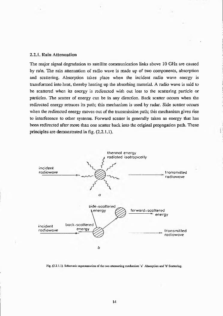
The major signal degradation to satellite communication links above 10 GHz are caused by rain. The rain attenuation of radio wave is made up of two components, absorption and scattering. Absorption takes place when the incident radio wave energy is transformed into heat, thereby heating up the absorbing material. A radio wave is said to be scattered when its energy is redirected with out loss to the scattering particle or particles. The scatter of energy can be in any direction. Back scatter occurs when the redirected energy retraces its path; this mechanism is used by radar. Side scatter occurs when the redirected energy moves out of the transmission path; this mechanism gives rise to interference to other systems. Forward scatter is generally taken as energy that has been redirected after more than one scatter back into the original propagation path. These principles are demonstrated in fig. (2.2.1.1).

thermal energy radiated isotropically

incidentradiowave transmitted

radiowave

a

s id p -f t rn tfp r p r lf orwa rd -sca t tered

energy

incidentradiowave

back-scattered energy > transmitted*o- , .radiowave

b

Fig. (2.2.1.1). Schematic representation of the two attenuating mechanism 'a' Absorption and 'b' Scattering.

14

Note that side scatter usually contains a component in either the forward direction or the back direction.

Mathematically the signal attenuation on a path, referred here as the extinction, is the algebraic sum of the components due to scattering and absorption [Allnutt, 1989]:

4. = 4*+4. (2-2. l.i)Where the subscripts ex, ab and sc refer to extinction, absorption and scattering respectively and Aex is the total attenuation or extinction along the path.

The relative importance of scattering and absorption is a function of complex index of refraction of the absorbing/scattering particles. Which is itself a function of signal wavelength, temperature and the size of the particles relative to the wavelength of the radio wave.

Theoretical models use scattering theory and adopt suitable values for the physical parameters such as shape and distribution of rain drops. To calculate the attenuation of a radio wave as it passes through rain it is necessary to aggregate individual extinction contribution of each rain drop encountered along the path. Since the drops are all of different sizes, it is necessary to introduce a drop size distribution Np> and integrate the extinction contributions as [Allnutt, 1989]:

Aex=4.343 xLjcm NDdD dB (2.2.1.2)0

Where OpD is the total extinction cross section of a diameter D and L is the length of the path through the rain. If the length of the path through the rain is set equal to 1 km, eq. (2.2.1.2) gives the specific attenuation , as:

7 = 4.343J CmNDdD dB/km (2.2.1.3)0

The characteristics of rain vary so much in both space and time that it is necessary to resort to either empirical methods or statistical averaging in order to reduce the range of the variables in the attenuation calculation procedures. Simple procedures, which are not always very accurate, can some times obtain results well within the accuracy achievable in most measurements. One such simplification is the power law relationship. So equation

15

(2.2.1.3) can be approximated in rain attenuation prediction models as:

y = aRb dB/km (2.2.1.4)

Where a and b are frequency dependent coefficients. In some rain attenuation models 7 is replaced by a (R) and a and b by k and a respectively (see chapter 3). In CCIR documents the above eq. (2.2.1.4) is written as [CCIR Rep. 564-4, 1990]:

The coefficients k and a have been calculated at a number of frequencies and are shown in Table (3.1.2).

2.2.2. Gaseous AttenuationGaseous attenuation is a molecular absorption process which results in amplitude

change in the rotational energy of the molecule and occurs at a specific resonance frequency or narrow band of frequencies [Ippolito, 1986].

Oxygen and water vapour have resonance frequencies in the bands of interest for satellite communication. Oxygen has a series of very close absorption lines near 60 GHz and an isolated absorption line at 118.74 GHz. Water vapour has lines at 22.3 GHz, 183.3 GHz and 323.8 GHz (fig. 2.2.2.1). The oxygen peak at 60 GHz is rather broad and actually consists of a closely spaced collection of absorption lines extending from around 57 to 63 GHz in all. The attenuation level within this is so severe that it renders communication through the atmosphere almost impossible. For this reason the 60 GHz band is being considered for inter-satellite links, certainly, where the communication environment is free from earth borne interference.

The attenuation produced by the resonance effects of water vapour and oxygen are described by the specific attenuation, in dB/km. The total atmospheric attenuation is found by integration of the specific attenuation value along the slant path, i.e

y = /cRa dB/km (2.2.1.5)

reduction of radio signals. This absorption of radio waves is caused by a quantum level

R

dB (2.2.2.1)0

16

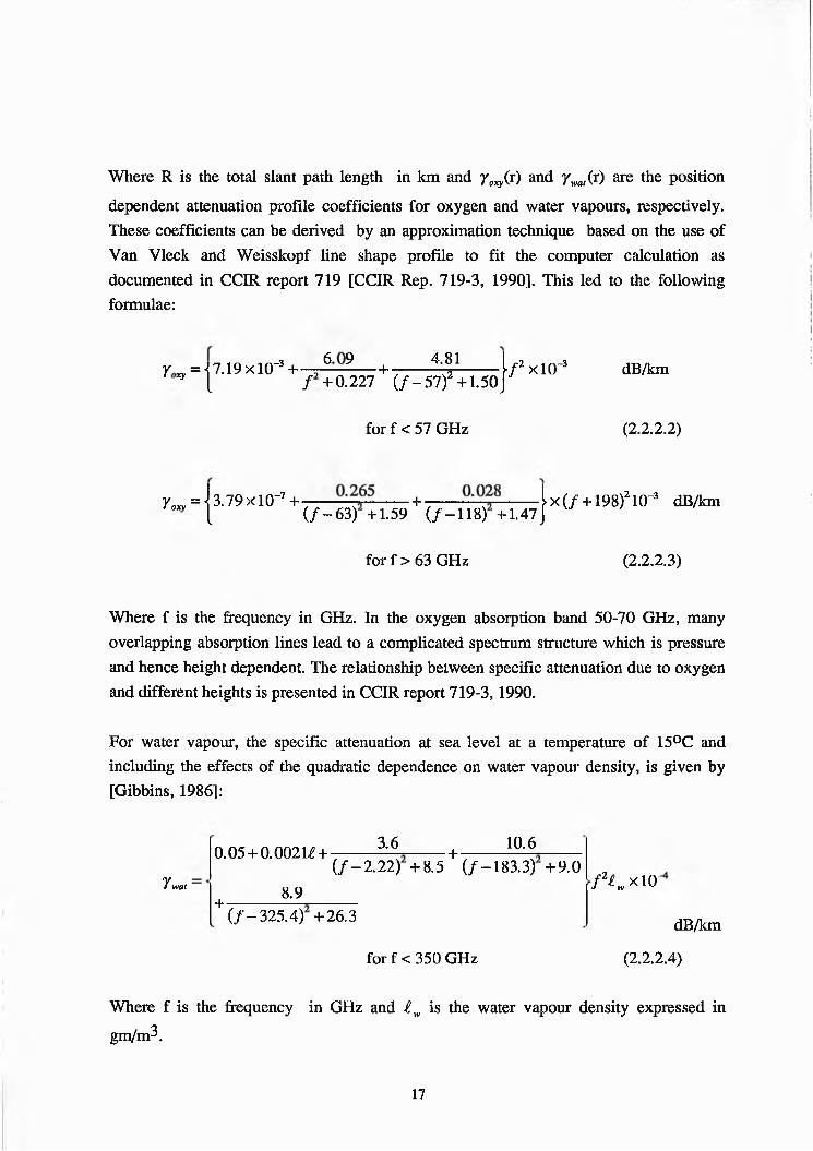
Where R is the total slant path length in 1cm and y oxy(v) and y wal(r) are the positiondependent attenuation profile coefficients for oxygen and water vapours, respectively. These coefficients can be derived by an approximation technique based on the use of Van Vleclc and Weisskopf line shape profile to fit the computer calculation as documented in CCIR report 719 [CCIR Rep. 719-3, 1990]. This led to the following formulae:

r = m 9 x l ( r 3 + ,6--9— •+----^ ----|/2xl0-3 dB/km^ I / +0.227 (/-57) +1.50J

for f < 57 GHz (2.2.2.2)

7„„ = j 3.79 x 1 O'7 + ------ +-- I x (/ +198)21 O'3 dB/km1 (/—63) +1.59 (y —118) +1.47 J

for f> 63 GHz (2.2.2.3)

Where f is the frequency in GHz. In the oxygen absorption band 50-70 GHz, many overlapping absorption lines lead to a complicated spectrum structure which is pressure and hence height dependent. The relationship between specific attenuation due to oxygen and different heights is presented in CCIR report 719-3,1990.

For water vapour, the specific attenuation at sea level at a temperature of 15°C and including the effects of the quadratic dependence on water vapour density, is given by [Gibbins, 1986]:

Y wat

0.05 + 0.002U + 3.6 ■ + 10.6(/-2.22) +8.5 (/-183.3) +9.0

+ 8.9(/-325.4) +26.3

/2/„x 10'

for f< 350 GHzdB/km

(2.2.2.4)

Where f is the frequency in GHz and £w is the water vapour density expressed in gm/m3.

17

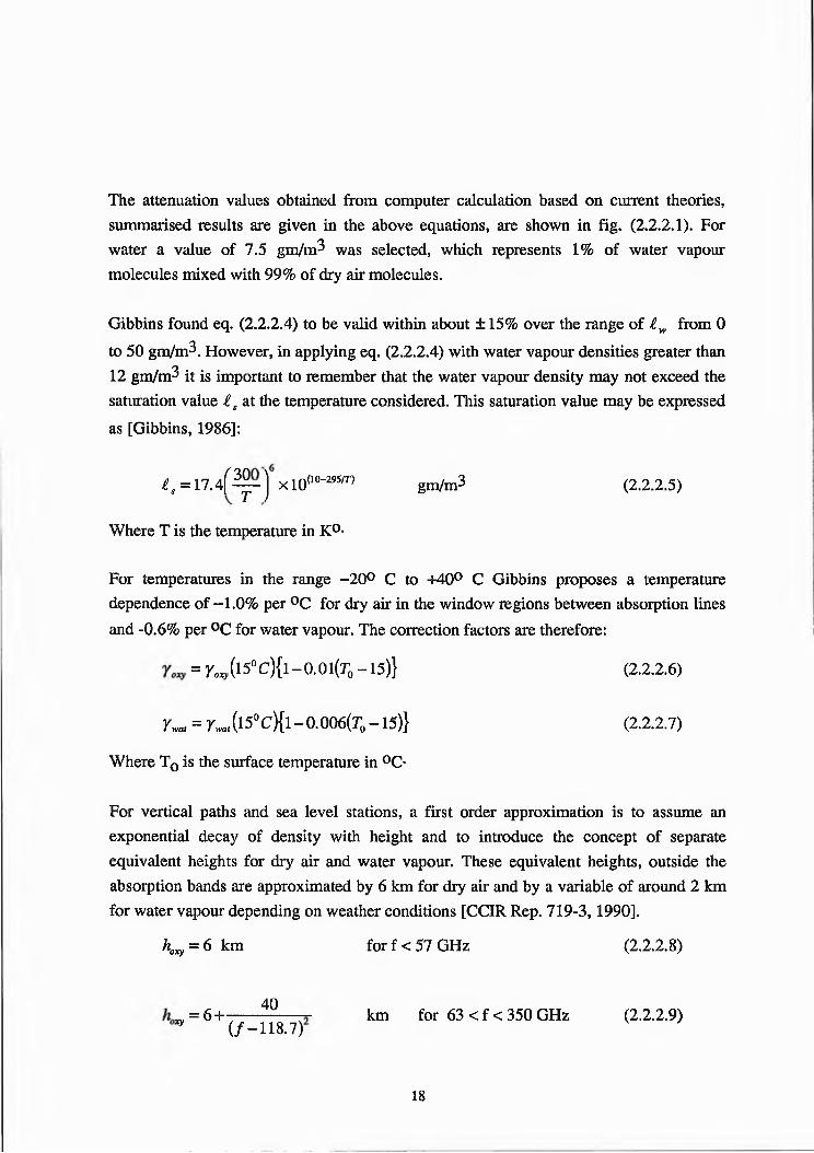
The attenuation values obtained from computer calculation based on current theories, summarised results are given in the above equations, are shown in fig. (2.2.2.1). For water a value of 7.5 gm/m8 was selected, which represents 1% of water vapour molecules mixed with 99% of dry air molecules.

Gibbins found eq. (2.2.2.4) to be valid within about ±15% over the range of £w from 0 to 50 gm/m8. However, in applying eq. (2.2.2.4) with water vapour densities greater than 12 gm/m8 it is important to remember that the water vapour density may not exceed the saturation value i s at the temperature considered. This saturation value may be expressed as [Gibbins, 1986]:

^ = 17-4f^r) X 1 0 " > gm/m 3 (2.2.2.5)

Where T is the temperature in K°-

For temperatures in the range -20° C to +40° C Gibbins proposes a temperature dependence of —1.0% per °C for dry air in the window regions between absorption lines and -0.6% per °C for water vapour. The correction factors are therefore:

= r J i 5°c){i-o.oi(r0 -15)} (22.2.6)

r™, = 7TO,(l5°c){l-0.006(7’0- 15)} (22.2.1)

Where T0 is the surface temperature in °C-

For vertical paths and sea level stations, a first order approximation is to assume an exponential decay of density with height and to introduce the concept of separate equivalent heights for dry air and water vapour. These equivalent heights, outside the absorption bands are approximated by 6 km for dry air and by a variable of around 2 km for water vapour depending on weather conditions [CCIR Rep. 719-3, 1990].

hoxy = 6 km for f < 57 GHz (2.2.2.S)

=6+ 40 km for 63 < f < 350 GHz (2.2.2.9)^ (/-118.7)

18

3.0 5.0 2.5 Ion(/ - 22.2)2 + 5 + (/ -183.3)2 + 6 + (/ - 325.4)2 + 4 for f < 350 GHz (2.2.2.10)

Wherehw is water vapour equivalent height in the window region hw = 1.6 km in clear air and hw = 2.1 km in rain.

These equivalent heights for water vapour were determined at a ground level temperature of 15° C. For other temperatures the equivalent heights may be corrected by 0.1% per °C in clear weather or rain respectively, in the window regions, and by 0.2% or 2% per °C in the absorption bands.

The concept of equivalent height is based on the assumption of an exponential atmosphere specified by a scale height to describe the decay in density with altitude. The scale height for both dry air and water vapour may vary with latitude, season and/or climate, and that water vapour distributions in the real atmosphere may deviate considerably from the exponential, with corresponding changes in equivalent heights.

As an example, the total one way zenith attenuation through the atmosphere is shown in fig.(2.2.2.2) [after CCIR Rep. 719-3, 1990]. This plot vividly points out the atmospheric regions where communications are practical and not practical. It is interesting to note that water vapour attenuation at 30 GHz is .25 dB and for 20 GHz is nearly .3 dB. The reason is that water vapour has resonance frequency at 22.3 GHz which is more closer to 20 than 30 GHz. The attenuation is 1 dB at 50 GHz, where as it rapidly increases to over 200 dB at the oxygen absorption band around 60 GHz.

2.2.3. Hydrometeor AttenuationHydrometeors are the products formed by the condensation of atmospheric water vapours and which cause reduction in radio wave signal amplitude. They exist in several distinct forms such as rain, fog, cloud, snow and ice. Attenuation through these media involves both absorption and scattering processes. Rain attenuation the most severe effect and is the major signal impairment to satellite communication links, particularly in the

19

frequency bands above 10 GHz. Attenuation due to dry ice particles is usually so low that it is insignificant for satellite communication links operating below 30 GHz.

2.2.4. Attenuation Due To Other FactorsThere are other sources of attenuation such as cloud and fog which contribute towards the signal degradation at ka band. Attenuation due to cloud of different types have been documented [Slobin, 1982] which were divided into twelve categories. The presence of clouds in space-earth down link antenna beams have two primary effects. Signal attenuation and an increase in system noise temperature. Stratocumulus cloud can cause total 0.24 dB signal attenuation at 20 and 30 GHz. On the other hand cumulus clouds, especially, large cumulonimbus and cumulus congestus can result approx. 3.8 and i.8dB total signal attenuation at 20 and 30 GHz, respectively.

Fog and mist are essentially supersaturated air in which some of the water has precipitated out to form small droplets of water. The droplets are usually smaller than 0.1 mm in diameter. Attenuation due to fog is a complex function of the particle size, distribution, density, extent, index of refraction and wavelength. A regression analysis on the theoretical attenuation which is good between wavelength 3 mm and 3 cm and for temperature between -8 < T < + 25 °C shows the variation of attenuation with temperature and wavelength [Altshuler, 1984]. For 20 and 30 GHz at 20° C the attenuation due to fog can be inferred from regression fit as 0.2 and 0.5 dB/km/gm/m3 respectively.

Cloud and fog attenuation at 20/30 GHz is very low compare to rain. When any communication system is designed having availability link margin for rain naturally incorporates the less severe attenuation due to other atmospheric effects. Therefore the cloud and fog signal impairment are not significant at ka band. However, clouds must be considered for systems with minimal margin that are intended for continuos use such as deep space link receiving unrepeatable spacecraft data.

2.3. S C IN T IL L A T IO N

Scintillation describes the condition of rapid fluctuation of the signal parameters of a radio wave caused by time dependent irregularities in the transmission path. Scintillation effects can be produced in both the ionosphere and the troposphere. Electron density irregularities occurring in the ionosphere can affect frequencies up to about 6 GHz

20

[Xppolito, 1986]. Scintillation occurring in the presence of rain are termed as wet scintillations.

The amplitude and phase of electromagnetic waves propagating through a turbulent medium, such as the troposphere, suffer from fluctuations caused by small variation of the refractive index. Amplitude scintillation of microwave signals received from a satellite show marked enhancement during hot weather [Merlo et al., 1985]. Maximum scintillation amplitude is generally reached when high temperature, humidity and atmospheric instabilities are present across the path. When the satellite signal is received at low antenna elevation angle, the radio path passes through a long atmospheric segment. These conditions further enhance the scintillation phenomenon which may cause severe impairment to telecommunication systems operating with a low fading margin.

2.3.1. Ionospheric Scintillations

In the ionospheric region of the earth free ions and electrons exist in abundance to affect the properties of electromagnetic waves that are propagated within and through it. Owing to a combination of gravitational forces and heating by the sun, the ionosphere will tend to move in a horizontal direction, much like the wind in the troposphere and stratosphere [Allnutt, 1989]. Since the ionospheric wind contains electrically charged particles and as it passes through the magnetic field lines of the earth, a current will be generated. The movement of this current is west to east at the geomagnetic equator, where the current is at a maximum. This peak current is referred to as equatorial electrojet and it flows at a height of about 110 km [Allnutt, 1989]. The generation of the current is at maximum on the side of the earth exposed to the sun.

Scintillation has primarily been considered only as a low frequency effect, however, ionospheric scintillation have been observed on microwave frequency links. Equatorial scintillation have been measured on INTELSAT satellite links at 6 GHz [Tuar, 1973],

2.3.2. Tropospheric Scintillations

When the troposphere is still, the refractive index varies slowly with height and even more slowly in the horizontal plane. Ray bending and the multipath at low elevation angels are likely to occur in these still air situations. The presence of wind makes the atmosphere to become mixed rather than stratified and causes relatively rapid variations

21

in refractive index to occur over small intervals. Earth station operating at low path elevation angles may encounter significant signal impairments due to tropospheric scintillation. Variation in the tropospheric refractive index may induce both amplitude and phase scintillations on slant paths under clear sky, cloudy or rainy conditions. Unlike ionospheric scintillation, the tropospheric scintillation effects increase as the frequency increases. This type of scintillation is caused by high humidity gradient temperature inversion layers. The effects are seasonally dependent, vary day to day and with the local climate.

The first tropospheric scintillation measurements at low elevation angels using a frequency above 1 GHz have been reported in Canada in 1970 by McCormick using the 7.3 GHz beacon from the US satellite TACSATCOM-1 [Allnutt, 1989]. TACSATCOM- 1 was drifting westerly and measurements were made over a period of 22 days. During the time, the satellite moved from an elevation angle of 6° to 0°. Two antennas, spaced 23m apart, were used for the experiment. The diameters of the antennas were 9m and 18m. The recorded data showed good correlation between the scintillations occurring along the paths, A typical data segment is shown in fig. (2.3.2.1)

GMT 1 November 1970

Fig. (2.3.2.1). Signal strength versus time for a 15 min period(a). 9 m antenna(b). 18 m antenna [after Allnutt, 1989J.

22

The presence of rain along the path was thought to reduce the amplitude of tropospheric scintillations significantly at all fade levels. Some measurements taken using OTS and INTELSAT V satellites have demonstrated that rain along the path produced no net reduction in the amplitude of the scintillations [Allnutt, 1989] [Karasawa et al., 1988], at least until the mean path attenuations were in excess of about 5 dB. Figure (2.3.3.1) shows the original and smoothed data with the net scintillations.

2.3.3. Wet And Dry Scintillations

20-10-m-o

S: o-

«- 2 0 -

-30' * * * * * -*-----■_time (2 min/div)

Fig. (2.3.3.1). Separation of atmospheric scintillation and rain attenuation using a moving 1 min averaging technique, 29th July 1982 [after Karasawa et al., 1988].(a). Original 11 GHz data at Yamaguchi.(b). Data smoothed by 1 min moving average.(c). Difference between original and smoothed data.

23

Supplementary analysis showed that the amplitude distribution of the same percentage of time the wet scintillation had a higher amplitude than dry scintillations [Allnutt, 1989].

2.3.4. Tropospheric Scintillations Characteristics

Although, the world wide data base is inadequate for long term measurement (more than 1 year), the general characteristics of tropospheric scintillation have been identified and summarised [Alluntt, 1989] as follows:(I). Meteorological dependence

A strong correlation is found in between temperature and humidity, that is, high temperature and high humidity give rise to high scintillation amplitudes for a given path. The presence of rain does not significantly effect the amplitude of the scintillations until the path attenuation exceed about 5 dB.(ii). Temporal dependence

Tropospheric scintillations are seasonally dependent. Variations occur diurnally. Peaks of activity are in the early afternoon and mid summer for temperate latitudes.(iii). Geographical dependence

As a significant correlation exists with temperature and humidity, thus there is a dependence on latitude. The higher the latitude, the colder is the average temperature of the atmosphere and so the lower will be the amplitude of scintillations over a given path.(iv). Frequency dependence

When the same antenna is used to measure the tropospheric scintillation at two, or more, frequencies high correlation have been reported [Karasawa et al., 1988].(v). Systematic dependence

Tropospheric scintillations are location dependent, they change with the change of earth station location. As the diameter decreases for a given path:

© Scintillation amplitude increases.

As the elevation angle decreases for a given location:

24

© Scintillation amplitude on average increases.© Period of scintillation increases.

Separation of diversity antennas horizontally by about 500 m effectively decorrelates the scintillation effect along the two paths. Separating the two antennas vertically produces a greater decorrelation than separating the same distance horizontally [Allnutt, 1989].

During 1975-76 , a number of experimenters undertook the opportunity to measure low elevation angle tropospheric scintillation effects at 20 and 30 GHz when the ATS-6 satellite was shifted to 35° East. Unfortunately, the limited observation time available did not allow to obtain any statistically meaningful results. In another experiment, high latitude measurements were made at frequencies 4 and 6 GHz at elevation angles down to 1° using signals from ANIK and LES satellites in Canada and INTELSAT and SYMPHONE satellites in Norway. All the measurements showed that the cold, less humid climate at high latitudes significantly reduced the tropospheric scintillation effects [Allnutt, 1989].

2.4. D E P O LA R IS A TIO N

Depolarisation occurs due to anisotropy of the propagation medium. If the medium (for example, rain) is composed of symmetrical particles (i.e. perfectly spherical raindrops), no signal depolarisation would occur. However the rain drop shape distorts owing to hydrodynamic forces. The drops not only become non-symmetrical in shape, but, also tend to be tilted away from the local horizontal and vertical axes of symmetry due to wind gusting in heavy rainstorms. Usually, a linearly polarised signal from a satellite is not aligned with the local vertical and horizontal axes of symmetry. This tilt of the incident electric vector away from the axes of symmetry of the rain drop causes signal depolarisation [Allnutt, 1989].

Depolarisation measurements have been made on terrestrial radio paths [Hogg et al., 1975] and have been extrapolated to provide estimates of depolarisation for earth space paths. The results manifest itself as cross talk between transmission made in orthogonally polarised channels. In ka frequency bands depolarisation effects are predominant due to hydrometeor, primarily rain and ice crystals.

25

2.4.1. Raimi DepolarisationRain induced depolarisation is generated by differential attenuation and differential phase shift in the incident radio wave caused by the non-sphericity of rain drops. As the rain drop size increases, their shape tends to change from spherical to oblate spheroid, eventually exhibiting a flattened or concave base [Pruppacher and Fitter, 1971]. Rain drops generally canted at angles with respect to the horizontal, hence the level of depolarisation experienced by the incident wave will be dependent on its polarisation with respect to the drop canting angles [Saunders, 1971; Oguchi, 1983].

Measurements taken from satellite beacon have shown that on average the vertically and horizontally polarised wave experience much less depolarisation than circular polarisation or linear polarisation at 45°. Maximum depolarisation is expected for signals which are circularly polarised and signals which are linearly polarised and oriented at an angle of 45° to horizontal [Cox et al., 1978; Arnold et al., 1978].

2.4.2. Ice DepolarisationIce is a very weak attenuator of radio waves compared to liquid water [Evans and Holt, 1977]. Ice particles (non-spherical crystals and snow flakes) were not considered seriously in earth-space propagation prior to early satellite beacon measurements even though their anisotropic differential phase shifting properties had been measured in the atmosphere using dual polarisation radar [McCormick and Hendry, 1977]. Earth space ice depolarisation was observed in the measurements by ATS-6 beacon [Bostain et al., 1975; Bostain and Allnutt, 1979] but was not identified as a significant propagation effect until the results obtained from the ATS-6 measurements in Europe and the CTS and COMSTAR measurements in USA. Winter observations [Arnold et al., 1977; Cox et al., 1978] confirmed that ice crystals and snow flakes are strong depolarisers.

2.5. R A D IO NO ISE

Radio noise, whether it is natural or man made, is considered to be a limiting factor in communication systems. The significant contribution which are likely to affect the ka band link performance originates from the sun or atmospheric gases. Noise from galactic sources and the background cosmic black body effective noise temperature of 2.7 K are of negligible significance relative to normal communications satellite usage within the geostationary orbit.

26

2.5.1. Solar Noise

The sun is a strong variable noise source offering an equivalent noise temperature of around 104 K at ka band [Meredith, 1987]. An outage may result at ground station whenever the sun crosses receiver antenna beam. These occasions are, obviously, of limited duration.

2.5.2. Atmospheric Gaseous NoiseAtmospheric gaseous noise is a molecular absorption phenomenon which results reduction in radio wave energy and offers a thermal noise power radiation. Oxygen and water vapours are major contributors to increase in radio noise from the atmosphere. [CCIR Rep. 720-2, 1990] provide plots of effective noise temperature or brightness temperature of the atmosphere as seen from a ground based receiver for various elevation angles. Figure (2.5.2.1), (2.5.2.2) and (2.S.2.3) show these curves for water vapour concentration levels of 3 gm/m , 7.5 gm/m9 and 17 gm/m9 corresponding to relative humidity of 17%, 50% and 98%, respectively. It can be seen that the shape of the curves closely resembles to zenith attenuation (see fig. 2.2.2.2). An expanded plot of relevant frequencies is shown in fig. (2.5.2.4) at 7.5 gm/m9 vapour concentration. The curves exclude the contributions due to black body cosmic radiation (2.7 K) and other extra­terrestrial sources.

2.5.3. Hydrometeor NoiseHydrometeor are water constituents found in the atmosphere in a solid or liquid states in the form of rain, snow, hail, clouds or fog. Unlike the gases where the absorption of microwave occurs by rotational and vibrational transitions of the molecules, in case of hydrometeors, the absorption occurs by reaction with the free and bound charged particles of the medium [CCIR Rep. 720-2, 1990] and this absorption, especially at higher frequencies, contributes to the emission of noise [Crane, 1971]. It is interesting to note that in hydrometeor absorption there is no resonance, but a continuous increase of attenuation with frequency until there is a saturation in the millimetre wave region.

As attenuation produced by rain is the most significant contribution to link degradation at ka band, so the increase in effective sky noise temperature due to rain causes much of the increase in system noise temperature of the satellite link. The noise power increase occurs simultaneously with signal loss due to fading and therefore a dual effect reduces

27

the overall carrier to noise ratio of the link. The following Table (2.5.3.1) shows the increase in system noise figure experienced with given depth of rain fade [after Ippolito, 1986].

Table (2.53.1)Increase in receiver system noise figure caused

by noise contribution from a rain fade.

Rain fade level

Noise due to rain

Effective noise figure for given j system noise figure (dB) |

(dB) °K 2170° K

3290°K

4438°K

6865°K

102610°K

1 56 2.50 3.41 4.32 6.21 10.083 137 3.12 3.92 4.74 6.48 10.205 188 3.47 4.21 4.98 6.65 110.2710 247 3.85 4.53 5.25 6.83 10.35

1 15 266 3.96 4.62 5.33 6.89 10.371 20 272 3.99 4.65 5.35 " . .6.91 10.381 30 274 4.01 4.67 5.37 6.91 10.39 1

28

29

< r

Z E N I T H A T T E N U A T I O N

Frequency (G i ls )

Figure (2.2.2.2)* T otal zenithal attenuation at ground level.

Pressure: 1013 mb

Temperature: 15°C

A for a dry atmosphere

B with water vapour; 7.5 g /m 3 at ground level.

J30

31

( f

8 8CM «—

OH 3 «n iV H 3 d lA I31 3SION-A>lS

o o ° ° .— co co cn

8CO

XO>

° z o *<-CM UJ3a

HiCCUL

t»0CniPO'-ua}>

.-C3CumO6«3f-i<DndO6cC

Po3(-<<yaa<yoa>»CO<Ncicrje<u!3bOfH

32

(>0 3U n iVy3dW 3JL 3SI0N-AM S

33

34

CHAPTER 3

RAIN ATTENUATION PREDICTION MODELS

Several models for estimation of cumulative attenuation statistics on the earth space paths have been developed. Each of these models appear to have advantages and disadvantages depending on the specific application. In this chapter an attempt is made to briefly discuss and summarise the key features of some of the well known rain attenuation models.

In the development of a rain attenuation prediction model the essential steps are described [Leitao et al., 1986] as:

© Characterisation of the statistical properties of rainfall and path attenuation onhorizontal paths, leading to determination of the rainfall rate reduction factor and an attenuation conversion factor for widespread and showery rain.

© Evolution of relationships between attenuation on horizontal and slant paths forwidespread and showery rain, including the effects of elevation dependence, melting band and variation in rain height.

© Climatic characteristics of rainfall types and freezing heights including the seasonal dependence of rain intensity and rain height.

® Determination of the freezing layer height during rain.

3.L CCIR RAIN ATTENUATION MODEL

The original CCIR procedure has undergone several modifications. The rain characterisation and attenuation prediction procedures described in this chapter are the latest version [CCIR Rep. 563-4 and 564-4, 1990].

The first element of the CCIR model involves a global map of fifteen rain climatic zones with associated rainfall intensity cumulative distributions for each specified region [CCIR Rep. 563-4, 1990]. Average annual rain rates are given for exceedance times from 0.001 to 1.0 percent. The global map of CCIR climatic zones are presented in fig. (3.1.1)

35

to (3.1.3), ranging from A (light rain) to Q (heavy rain). Table (3.1.1) lists the rain rate distribution for the fifteen rain climatic zones.

The CCIR model assumes that the horizontal, extent of the rain is coincident with the ambient 0° C isotherm height. An average value of 0° C isotherm height is used in the CCIR model, obtained from [CCIR Rep. 564-4, 1990]

hR - 3.0 + 0.028(0) O<0<36° 1cm (3.1.1)

hR = 4 .0 - 0 .075(0-36) <p >36° 15111 (3.1.1 A)

Where hR is the effective rain height in km and 0 is the latitude of the location of earth station in degrees. The geographical location of Guildford is 51.25° N and 0.3° W, hence the effective rain height is:

hR =2.86 km (3.1.1a)

slant path length, Ls, for 0 > 5° can be obtained from figure (3.1.4) as:

L (A/lzM lcm (3.1.2)sin a

For 0 < 5, a more accurate formula should be used:

2 { h ,-h s)

sin2+ 2 (hR- h skm (3.1.3)

R.+ sin0

)

Where Re is the effective radius of earth ( 8500 km), hs is the earth station height above sea level in km and 0 is elevation angle in degrees. Equation (3.1.2) is applicable to University of Surrey measurement site since 0=28.8°. The earth station height, hs, is

0.07 km also using eq. (3.1.1a) gives slant path length as:

Ls = 5.78 km (3.1.2a)

The horizontal projection, LG, of the slant path length is found from fig.(3.1.4) as:

Lg - LsCos0 km (3.1.4)

Substituting the value of Ls and 0 from above equations gives

36

Lg = 5,07 km (3.1.4a)

The rain intensity, , exceeded for 0.01% of an average year can be obtained from the

CCIR maps [CCIR Rep. 563-4,1990] as shown in fig. (3.1.2). Guildford falls in zone E of CCIR global climatic division maps, table (3.1.1) gives

^ 0 ^ = 2 2 mm/hr (3.1.4b)

The reduction factor, rQ.oi* f°r 0.01% of the time, which adjusts the effective rain height of slant path corresponding to different rain rates, can be calculated from [Yamada et al., 1987]:

^01= — T ~ r (3-1-5)1+ %/ b'o

Where L0 is the characteristic length of a rain cell and is given as:

L„ = 35 exp(-0.015/?aol) (3.1.5a)

Utilising eq. (3.1.4b) and (3.1.5.a) in eq. (3.1.5) yields:

r001 = 0.83 (3.1.5b)

The specific attenuation, jp , exceeded for 0.01% of an average year is given by the following equation:

YP = k(Roo,)0 dB/km (3.1.6)

Where k and a are frequency dependent coefficient. These coefficients have been calculated at a number of frequencies between 1 and 1000 GHz for several drop temperatures and drop size distribution [Olsen et al., 1978]. For linear and circular polarisation, the coefficients in eq. (3.1.6) can be calculated from the values in Table(3.1.2) by using the approximate eq. (3.1.7) and (3.1.8) given below [CCIR Rep. 721-3,1990]:

_ [kH +kv + (kK - K )C os2eCos2T]2

37

\kHa H +kva v +(kHa H - kva v)Cos26Cos2t ]

(3.1.8)

Where 0 is the path elevation angle and x is the polarisation tilt angle relative to the horizontal (x=45° for circular polarisation). The subscripts H and V represent horizontal and vertical polarisation, respectively.

If the desired frequency, f, is intermediate between frequencies (say f j and f2 ) in Table(3.1.2) kH, kv and a H and a v can be interpolated in the following way (f2 > fi):

Wherelatgg = Latitude of the earth station in degrees.l°ndi = Difference between satellite and earth station longitude in degrees.

Guildford ground station location is given earlier as 51.25° N and 0.3° W. Olympus satellite is in the geostationary orbit location of 19° W. Thus for the Olympus the polarisation tilt angle is calculated as:

log * = (log *2 - log A lQgjl + log /qlog / 2- log f

(3.1.7a)

a = (a2- a ]) log f ~ log f\ ] a log f i - log fi

(3.1.8a)

The polarisation tilt angle,x, is obtained from the following equation (3.1.9):

(3.1.9)

T = 14.23° (3.1.9a)

For 20 G H z: =0.0751

a H =1.099

k = 0.07412 a = 1.10

a v = 1.065

=0.0691

38

The specific attenuation, y , exceeded for 0.01% of an average year can be calculated

from eq. (3.1.6) as:

y001 = 2.22 dB/km (3.1.6a)

The total rain attenuation exceeded for 0.01% of an average year may then be obtained from:

A.oi ~ To.oiAs o.oi tiB (3.1.10)

Using the values y001, Ls and r001 from equations (3.1.6a), (3.1.2a) and (3.1.5b)

respectively gives rain attenuation as:

Am =10.65 dB (3.1.10a)

The attenuation to be exceeded for other percentages of an average year, in the range 0.001% to 1.0% is estimated from the attenuation to be exceeded for 0.01% for an average year by using :

A_ Q n p - i 0 M ^ O&P)

4™ (3.1.11)

The CCIR reports that when the above prediction method was tested the results differed between high and low latitudes. For latitudes above 30°, the prediction was found to be in good agreement with available measured data in the range 0.001% to 0.1% with a standard deviation of some 35% when used with simultaneous rain rate measurements. Figure (3.1.5) shows CCIR prediction for Guildford.

Table (3.1.1)CCIR rain climatic zones.

Rainfa 1 intensity exceeded (mm/hr)% A B c D E F G H J K L M N P1.0 < .1 0.5 0.7 2.1 0.6 1.7 3 2 8 1.5 2 4 5 12 240.3 0.8 2.0 2.8 4.5 2.4 4.5 7 4 13 4.2 7 11 15 34 490.1 2 3 5 8 6 8 12 10 20 12 15 22 35 65 72.03 5 6 9 13 12 15 20 18 28 23 33 40 65 105 96.01 8 12 15 19 22 28 30 32 35 42 60 63 95 > 115.003 14 21 26 29 41 54 45 55 45 70 105 95 140 200 142.001 22 32 42 42 70 78 65 83 55 100 150 120 180 250 170

39

Table (3.1.2)Regression coefficients for estimating specific attenuation [after CCIR Rep. 721].

Freq. (f) GHz Kh Kv «//

1 0.0000387 0.0000352 0.912 0.8802 0.000154 0.000138 0.963 0.9234 0.000650 0.000591 1.121 1.0756 0.00175 0.00155 1.308 1.2657 0.00301 0.00265 1.332 1.3128 0.00454 0.00395 1.327 1.31010 0.0101 0.00887 1.276 1.26412 0.0188 0.0168 1.217 1.20015 0.0367 0.0335 1.154 1.128 - |20 0.0751 0.0691 1.099 1.06525 0.124 0.113 1.061 1.03030 0.187 0.167 1.021 1.00035 0.263 0.233 0.979 0.96340 0.350 0.310 0.939 0.92945 0.442 0.393 0.903 0.89750 0.536 0.479 0.873 0.86860 0.707 0.642 0.826 0.82470 0.851 0.784 0.793 0.79380 0.975 0.999 0.769 0.76990 1.06 0.999 0.753 0.754100 1.12 1.06 0.743 0.744120 1.18 1.13 0.731 0.732150 1.31 1.27 0.710 0.711200 1.45 1.42 0.689 0.690300 1.36 1.35 0.688 0.689400 1.32 1.31 0.683 0.684

40

3.2. CRANE RAIN ATTENUATION MODEL

This model is a regional model presenting the expected rain rate distribution for each region. The intent of the model is to provide a procedure for prediction of attenuation distribution and its possible variation at any point within the region [Crane, 1978]. The latter form [Crane, 1980] includes path averaging and adjusts the isotherm height for various percentages of time to account for the types of rain structures which dominate the cumulative statistics for the respective percentage of time.

The model provides median distribution estimates for broad geographical regions. Eight climate regions A through H are designated to classify regions covering the entire globe. Figure (3.2.1) and (3.2.2) show the geographic rain climate regions for the continental and ocean areas of the earth. The first step in the application of this global attenuation prediction model is the estimation of the instantaneous point rain rate, Rp, distribution. The values of Rp may be obtained from the rain rate distribution curves of fig. (3.2.3), however, the numerical values are tabulated for all regions in Table (3.2.1).

Table (3.2.1) [after Ippolito, 1989]

Rain rate distribution value (mm/hr) for Crane model.

Rain climate regions% of year A B C D E F ! G H

0.001 28.5 54.7 78 108 165 66 185 2530.002 21 44 62 89 144 51 157 220.50.005 13.5 28.5 41 64.5 118 34 120.5 1780.01 10 19.5 28 49 98 23 94 1470.02 7.0 13.5 18 35 78 15 72 1190.05 4.0 8.0 11 22 52 8.3 47 860.1 2.5 5.2 7.2 14.5 35 5.2 32 640.2 1.5 3.4 4.8 9.5 21 3.1 21.8 43.50.5 0.7 1.9 2.7 5.2 10.2 1.4 12.2 22.51.0 0.4 1.3 1.8 3.0 6.0 0.7 8.0 12.02.0 0.1 0.7 1.1 1.5 2.9 0.2 5.0 5.2

41

The atmospheric temperature decreases with height, and above some height, the precipitation particles becomes ice. The ice does not produce significant attenuation, however, the regions with liquid water precipitation particles are of interest in the estimation of attenuation. Measurement made using weather radar [Crane, 1982] show that the reflectivity of a rain volume may vary with height but, on average, the reflectivity is roughly constant with height to the height of 0° C isotherm and decreases above that height. The rain rate may be assumed to be constant to the height of the 0° C isotherm at low rates, this height may be used to define the upper boundary of the attenuating region. A high correlation between the 0° C height and the height to which liquid rain exists in the atmosphere should not be expected for the higher rain rates because large liquid water droplets are carried aloft above the 0° C height in the strong updraft cores of intense rain cells [Ippolito, 1989].

The following are the required input parameters for Crane global rain attenuation prediction model:

f: Frequency (GHz)0: Elevation angle to satellitehs: Ground station height above mean sea level (km)

<|): Ground station latitude (degrees)

Guildford lies in climate zone C of the Crane global rain distribution maps. For different percentage of an average year the rain rate distribution values can be taken from Table(3.2.1). The rain layer height from the height of the 0° C isotherm hR at the path latitude can be worked out from fig. (3.2.4). For the values of other percentages which are not shown in this fig. (3.2.4) can be interpolated. The horizontal path projection, L,G of the

slant path length can be found from fig. (3.1.4) as:

L0 = — ~ — km (3.2.1)tan 0

Where hR - h R(p) is the height of isotherm for probability p in km, hs is the ground station elevation above sea level in km and 0 is the elevation angle to satellite in degrees.

42

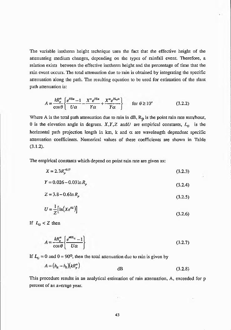
The variable isotherm height technique uses the fact that the effective height of the attenuating medium changes, depending on the types of rainfall event. Therefore, a relation exists between the effective isotherm height and the percentage of time that the rain event occurs. The total attenuation due to rain is obtained by integrating the specific attenuation along the path. The resulting equation to be used for estimation of the slant path attenuation is:

kR“A = — p-

,UZa -1cos 6 Ua

XaeYZa XaeYL(/x + ■Ya Ya

for 0>1OC (3.2.2)

Where A is the total path attenuation due to rain in dB, Rp is the point rain rate mm/hour, 0 is the elevation angle in degrees. X,Y,Z andU are empirical constants, LG is the

horizontal path projection length in km, lc and a are wavelength dependent specific attenuation coefficients. Numerical values of these coefficients are shown in Table(3.1.2).

The empirical constants which depend on point rain rate are given as:

-0.17X = 2 3 R

Y = 0.026 — 0.03 In R„

Z = 3.8~0.61n i?

£/ = i[ ln (X e K )]

If LG < Z then

(3.2.3)

(3.2.4)

(3.2.5)

(3.2.6)

!di“ [ eceL‘— P

cos 6 I U a

If Lg = 0 and 0 = 90°, then the total attenuation due to rain is given by

A = (ht -h s){kR°) dB

(3.2.7)

(3.2.8)

This procedure results in an analytical estimation of rain attenuation, A, exceeded for p percent of an average year.

43

The model described above has been used for rain attenuation prediction for Guildford. The result obtained is presented in fig. (3.2,5).

3.3. THE SIMPLE ATTENUATION MODEL

The Simple Attenuation Model (SAM) is a rain attenuation prediction model. It can be used to obtain rain attenuation statistics on earth space communication links operating in 10-35 GHz band. Previously this model was known as Piecewise uniform model. The latest SAM [Stutzman et al., 1986] includes the effect of wave polarisation. Simple calculations produce attenuation values as a function of average rain rate. These together with rain rate statistics (either measured or predicted) can be used to predict annual rain rate attenuation statistics.

The SAM [Stutzman and Dishman 1982 and 1984] is a semiempirical model. It is basedon an effective rain rate profile that is exponential in shape. The model consists of threeparts:

© The relationship between specific attenuation and rain rate.• The statistics of point rainfall intensity.© The spatial distribution of rainfall.

The specific attenuation can be related to rainfall rate by the following power law:

Since this model is for average yearly rain attenuation, measured average rainfall rate statistics for the earth terminal site should be used [Stutzman et al., 1986]. If these are unavailable, the CCIR rain rate model [CCIR Rep. 564] can be used. The SAM describes spatial rainfall distribution along the slant path, (/), as :

y(R) ~ I<Ra dB/km (33.1)

*(/) = *. Ra < 10 mm/hr (3.3.2)

Ra > 10 mm/hr

for I < Ls, where Ls is the slant path length given in eq. (3.1.2) as:

(3.3.3)

f a - a )s sin 6 (3.3.4)

44

Rq mentioned in the above equations is the point rain fall intensity in (mm/hr), hs is the earth station altitude in km, 0 is the slant path elevation angle in degrees, ! is a parametercontrolling the decay rate of horizontal rain profile and hR is the effective rain height inkm and approximated as:

h* = h‘ Ra < 10 mm/hr (3.3.5)

hR — + l o g R0 > 10 mm/hr (3.3.6)

Where h[ is the 0° C isotherm height in km.

The height of 0° C isotherm depends primarily on latitude. The dependence of height on latitude is approximated in [Crane, 1978] as:

^ = 4-8 km I0l< 30° (3.3.7)

^ - 7.8-0.1101 km I0I>3O<? (3 3 3 )

Where (j) is the latitude in degrees. The total attenuation due to a point rainfall rate R0 is found by integrating eq. (3.3.2) and (3.3.3) over the path integral

(3.3.9)

Evaluation of this integral yields the final expression:

A(Ra) = kRaaLs Ro < 10 mm/hr (3.3.10)

1 - expf- a t ln(/? / 10)Ln cos 0]A(RJ = / < PL ’ s------ 1 R > 10 mm/hr (33.11)

aq\n(R0 /lO )cos0

Where k and a specific attenuation coefficients for spherical rain drops [Olsen et al., 1978] and the path length, Ls, is given by eq. (3.3.4).

The only remaining undefined parameter in eq. (3.3,11) is The value of ^ in the original SAM model with spherical rain drop specific attenuation coefficients was 1/22. After changing the specific attenuation coefficients which includes the polarisation state, the value of £ was optimised with the expanded data base. A value ^=1/14 was found to

-give the best fit to different data sets for which both attenuation and rain rate data were

45

available. The functional dependence is such that large changes in t; do not produce large changes in attenuation [Stutzman et al., 1986]. This model has been used for rain attenuation prediction for Guildford at 28.8° elevation angle as shown in fig. (3.3.1). The dashed curve has been achieved using model parameter, £=1/22 while the optimised value of ^ has been utilised in obtaining the continuos curve. The figure shows that the low value of £ produced slightly higher attenuation value for low percentage of year.

3.4. LIN RAIN ATTENUATION MODEL

The set of empirical formulas presented here for earth satellite path attenuation is an extension of terrestrial microwave radio paths. First the terrestrial microwave radio path will be discussed briefly and later it will be extended to the earth satellite path attenuation.

In the case of terrestrial paths, the calculation of the expected rain attenuation distribution from a long term (>20 years) distribution of 5 minute point rain rates were accomplished using empirical formulas deduced from rain rate and rain attenuation measured data at five different locations in United States of America on nine radio paths (5-43 km) at 11 GHz [Lin, 1978]. These empirical formulas for terrestrial paths are:

y(R) = kRa dB/km (3.4.1)

A{R,L) = y (R )x L x dB (3.4.2)1 + -=/

L(R)

L(R) = 2636R -6 .2

km (3.4.3)

R is the 5 minute point rain rate in mm/hr, L is the radio path length in km, A(R, L) is the path rain attenuation in dB at the same probability level as that of R, the parameters lc and a are functions of the radio frequency, rain temperature and drop size distribution [Olsen et al., 1978].

If the rain rates were uniform over a radio path of length L, the path rain attenuation (R,L) woukL bs^jmply, -Y(R)L, representing a linear relationship between A and L.

46

However actual rainfalls are not uniform over the entire radio path and therefore the increase of A(R, L) with L is non-linear.

Two factors in the empirical method account for the radio path averaging effect. First, the method is based upon the long term distribution of 5 minute point rain rates in which the 5 minute time averaging partially accounts for the fact that the radio path performs a spatial averaging of non-uniform rain rates. The 5 minute average of the rain rate seen at a point corresponds to spatially averaging approximately 2.1 km of vertically variable rain rates, assuming 7 meters/sec. average descent velocity of rain drops [Ippolito, 1989].

If the radio paths of interest are longer than 2.1 km, the fixed 5 minute average interval can not adequately account for all the path length variations. This deficiency is compensated by the factor

l- j - (3.4.4)1+-=F—

U R )

To extend the method to earth satellite paths, the height of the freezing level (hR) in the atmosphere be the long term average rain height measured relative to sea level. The effective average length of the earth satellite path affected by rain is then

, (hs ~hs)Ls = . J km (3.4.5)

smo

Where 0 is the satellite elevation angle as viewed from the earth station in degrees and hs is the ground elevation measured from the sea level in km. The radar measurements of rainfall reflectivity have revealed that on the average rainy day hR is given as [CCIR Rep. 564-3, 1986]:

hR- 4 km (3.4.6)

Thus given the elevation angle 0, the ground elevation hs and the distribution of 5 minute point rain rates, the rain attenuation on the earth satellite path can be calculated through the use of eq. (3.4.1), (3.4.2) and (3.4.5). These formulas are valid only on the long term average. The short term relationship between the surface point rain rate and the earth satellite path rain attenuation, on a storm by storm basis, have been observed to be erratic and difficult to predict [Lin, 1978].

47

This model has been used for the attenuation prediction for Guildford as shown in fig.(3.4.1). Two values of effective rain heights has been used in the model for rain attenuation prediction. The solid line has been obtained with effective rain height value of 4 km as recommended [Lin, 1978] and the dashed line presents the rain attenuation for Guildford with effective rain height value of 2.86 km [CCIR Rep. 564-4, 1990]. Fig.(3.4.1) clearly shows the difference of effective rain height on signal attenuation level. The value, hR, of 4 km gives much higher attenuation at low percentage of time; while using the CCIR equation for hR the rain attenuation along the radio path are more comparable to other models.

3.5. COM PARATIVE EVALUATION OF MODELS

A number of rain attenuation prediction models have been developed. Some of those are semi empirical in nature. These models have been compared to different measured data which revealed that one model performed better than others and showed good correlation with the measured data at one percentage of time while the other model yielded better performance at different percentage of time. In this section a comparative evaluation of these models is presented.

All rain attenuation prediction models require long term measured rainfall intensity for different percentage of time for the final computation of attenuation. The CCIR and Global models are more independent in world wide application as no measured rainfall data for prediction of rain attenuation is required. These models have divided the world into different climatic zones. However, long term measured rainfall data is recommended for more accurate predictions.

A comparative evaluation of CCIR and Global models is presented [Crane, 1985]. In this evaluation study rain rate distribution of one or more than one years of observations at 52 locations were employed. The comparison have shown that the Global model performed better than the CCIR model for world wide application.

The Simple attenuation model has been tested [Stutzman et al., 1986] against the measured data bases of 62 experiments performed in the United States of America, Europe and Japan. A subset of 36 experiments were used for the optimisation of model parameter, The value of £ in the original SAM model was 1/22 which has been

48

optimised to 1/44. Using the optimised value of ^ yielded best fit to 36 data sets. In this study of evaluation the CCIR and Global models were also incorporated.

In first comparison the measured attenuation and rain data were used and deviation or difference between predicted and measured attenuation was computed on a percentage basis. This indicated that SAM provided the best fit to the data base but all three models performed well. These data were examined for three frequency bands (below 15, 15 to 25 and above 25 GHz) and similar results were obtained. This might be expected since the model parameter t, was optimised against that set of data. For the second comparison the data set of 62 sites were selected and predicted rather than measured rain rate was used. All these three models showed larger deviations. The large deviations resulted due to the fact that predicted rather than measured rain rate was used. The overall performance results revealed that the SAM yielded the best results. The Global model was slightly better for high percentages, but it was poor for low percentages. The CCIR model was better than SAM for low percentages but it was poor for high percentages. Furthermore all these models gave better predictions for long term (> 2 years) rather than short term (about one year) data sets.

A comparison of measured and predicted rain attenuation using Lin rain attenuation model have been made [Lin, 1978] for different frequencies and elevation angles in United States of America. The point rain rate distribution of 5 minute for 20 years were used for rain attenuation prediction. Two beacon measured data of 1 year, COMSTAR 19 GHz and 28.56 GHz and CTS 11.7 GHz, and radiometer data at 13.6 GHz of 1 year and 17.8 GHz of 2 years were used. The comparison revealed that there was close agreement between calculated results and measured data. The effective rain height, hR, of 4 km provided good approximation for eastern USA. The small differences between the measured and the calculated results for different earth stations might have been caused by the factors mentioned [Lin, 1978] below:

© The measured attenuation data (1 to 2 years) were shorter than those (20 years) of point rain rate data.

© The value of hR might not be exactly 4 km and may vary slightly from one location to another.

49

Lin rain attenuation model is valid only as a long term average. The short term relationships between the surface point rain rate and the earth satellite path rain attenuation, on storm by storm basis, are erratic and difficult to predict [Lin, 1978].

The models described above have been used for rain attenuation prediction for Guildford. CCIR rain climatic zones have also been employed for SAM and Lin rain attenuation model. In the case of SAM two values of model parameter ^ (1/22 and 1/44) were utilised and the Lin model predictions have been made with two different effective rain heights. The model itself employed an average value of 4 km. However, the effective rain height for Guildford has been estimated using the latest CCIR model equation [CCIR Rep. 564-4, 1990] as 2.86 km.

The above described models have been used for a comparative study of rain attenuation prediction for Guildford. Different rain attenuation prediction curves obtained, for 20 GHz at 28.8° elevation angle using CCIR climatic regions, are shown in fig. (3.5.1). All models yielded comparable attenuation values at high percentage of time and gradually departed towards low percentage of time. The CCIR, SAM and Lin (with effective rain height of 2.86 km) rain attenuation models show good correlation upto 0.01% of an average year and for 0.001% of time the Lin model prediction of attenuation due to rain is much higher than the CCIR and SAM results. On the other hand a good correlation exists between Lin (with effective rain height of 4 km) and Crane model predictions for Guildford. However for 0.001% of time the Lin model attenuation prediction is not only higher than Crane's but also higher than rest of the models.

The CCIR, SAM and Lin (with effective rain height of 2.86 km) models have shown good correlation of attenuation prediction because CCIR global rain maps have been used in these three models. In the second comparison, global rain maps as described by Crane [Crane, 1980] have been used for SAM and Lin rain attenuation prediction models for Guildford. Results are shown in fig. (3.5.2) which reveals SAM and Lin attenuation prediction are moving away from the CCIR attenuation prediction, this was expected, since Crane and CCIR global rain maps have different regional rain distribution. It would be interesting to compare the rain attenuation prediction of all these models with long term observed rain and beacon measured data.

50

<? '

165® 115* 105® 15* 45® ti®

Figure (3.1.1). CCIR climatic zones.

L — ............

51

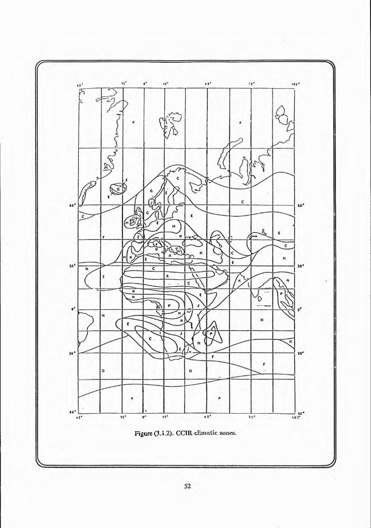
Figure (3.1.2). CCIR climatic zones.

53

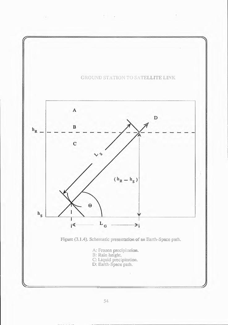
GROUND STATION TO SATELLITE LINK

Figure (3.1.4). Schem atic presentation o f an Earth-Space path.

A: Frozen precipitation.B: Rain height.C: Liquid precipitation.D: Earth-Space path.

54

( T

C C IR RAIN A TT EN U A TIO N M O D E L

0.001 0 .0 1 0 .1 1 P e rc e n ta g e o f a n a v e rag e y e a r a t t e n u a t io n e x c eed ed

Figure (3.1.5). Application of CCIR rain attenuation model for Guildford.

V : J

55

< r

uxncw

©w©

8 ©2 $

CD I

S B

0 0

2:o 2

< CD

0 0

d V IO d

V

o><DQLLIQ3H;O2O

oco

oCM

c6X>_oO

<NC O

o:3E

oCO

(6aa) 3 a n in v j

J56

< r

UVlOd

<1) ■ — 5 <

0 0

a |

< 00 0 0

d V lO d

O)d)QIDOID

CD2O

oCM

bOC"3ss

.2'3i -

-Qjd3CM

CM*CO<u£M\U

(6aa> aan i i iv i

V^= J57

R A IN R A T E D IS T R IB U T IO N C U R V E S

O.OOI 0 . 0 1 0 . 1 1P e r c e n t a g e o f year rain r a t e v a l u e exceeded

Figure (3.2.3). Rain rate distribution for all regions.

< r

C R A N E R A IN A T T E N U A T IO N P R E D IC T IO N

P e rc e n ta g e o f a n a v e rag e y e a r a t te n u a t io n ex ceed ed

Figure (3.2.5). Application of Crane rain attenuation model for Guildford.

J

60

< r

S IM P L E A T T E N U A T IO N M O D E L P R E D IC T IO N

0.001 0.01P e rc e n ta g e o f a n av e rag e

0.1 1a t te n u a t io n

Figure (3.3.1). Application of SAM model for Guildford.

61

( T =%

L IN R A IN A T T E N U A T IO N P R E D IC T IO N

0.001 0.01 0.1 1 P ercen tag e of an average y ea r a tte n u a tio n exceeded

Figure (3.4.1). Application of Lin rain attenuation model for Guildford.

J

62

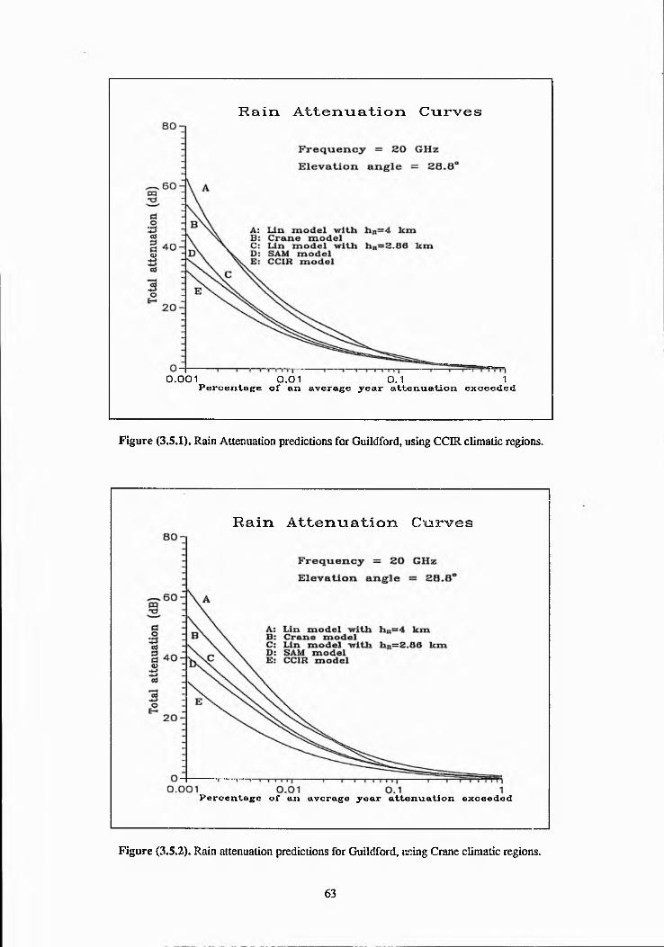
R a i n A t t e n u a t i o n C u r v e s

0 . 0 0 1 0 . 0 1 0 .1 1P e rc e n ta g e o f a n av e rag e y e a r a t te n u a t io n ex ceed ed

Figure (3.5.1). Rain Attenuation predictions for Guildford, using CCIR climatic regions.

Rain Attenuation Curves

P e rc e n ta g e of a n average y e a r a t te n u a t io n ex ceeded

Figure (3.5.2). Rain attenuation predictions for Guildford, using Crane climatic regions.

63

CHAPTER 4

MODIFICATION IN THE EXPERIMENTAL ARRANGEMENT FOR ka BAND MEASUREMENTS

In order to monitor the B j beacon signal an experimental arrangement was developed which is described in this Chapter. The Olympus signal was measured by extracting the beacon signal from front end of the CODE terminal as explained in Chapter 1. The B\ signal of 19770.39357 MHz (some times referred as 20 GHz) is then translated to 70 MHz IF by implementing a second down converter (see chapter 1 figure 1.4.1). The weather data was also recorded to observe the effects of rain on radio wave signal at 20 GHz.

A L OLYMPUS BEACON PAYLOAD

The 20/30 GHz Olympus payload was eagerly awaited by many experimenters and scientists. The complete beacon payload or package is providing a unique opportunity to users to carry out long term statistical evaluation of radio wave propagation at 12.5, 20 and 30 GHz. This also provides the first opportunity of radio wave propagation measurements at ka frequency band in Europe after ATS-6 since 1975-76. As the modelling of the dependence on the climatic and meteorological parameters is a prime requirement, a programme of intense co-operation and information exchange has been set up under the name of OPEX (Olympus Propagation Experiments).

A block diagram of the Olympus beacon payload is shown in fig. (4.1.1) and the foot print of beacon B^and B2 is given in fig. (4.1.2).

4.2, OLYMPUS LINK BUDGET

The European Space Agency (ESA) launched Olympus in geostationaiy orbit in July 1989 to carry out various experiments regarding the feasibility of future earth space communication links in ka band. On board is a beacon package having three beacon signals for propagation studies. The three beacons 12.5, 20 and 30 GHz are referred as B0> and B2 respectively. The 20 GHz is a switched beacon signal switching between two orthogonal polarisations, horizontal and vertical, with a rate of 1866 Hz. The link budget for the 20 GHz is given in table (4.2.1) and 30 GHz link budget is presented in Table (4.2.2). In these tables some of the figures were taken from [ESA Doc., 1990] and

64

calculations were performed using link budget equations [Morgan, et al., 1988; Evans, 1991].

Table (4.2.1)Link budget for Olympus beacon B \

Earth station location (Guildford) 51.24° N, 0.58° WEarth station antenna 1.2 m (diamond shape)Down link frequency 19770.3935 MHz !Signal polarisation Horizontal and VerticalPolarisation switching cycle 933.000525 HzFrequency stability over 24 hrs ±2 KHzFrequency stability over any year ±60 KHzFrequency stability over 7 years ±200 KHz JSatellite beacon EIRP 31.7 dBW JEIRP Variation:Over any 1 second ±0.05 dBOver any 24 hrs ±0.5 dBOver any year ±1.0 dBOver 7 years ±2.0 dBEarth station antenna gain 46.4 dBFree space path loss 210.2 dBEarth station G/T 26.4 dB/k

O N o ......... 68.8 dB Hz |Power received at ground station -139.8 dBW !

65

Table (4.2.2)Link budget for Olympus beacon B2 .

Earth station location (Guildford) 51.24° N, 0.58° WEarth station antenna 1.2 m (diamond shape)Down link frequency 29655.5915 MHzSignal polarisation VerticalFrequency stability over 24 hrs ±3 KHz

Frequency stability over any year ±90 KHzFrequency stability over 7 years ±300 KHzSatellite beacon EIRP 27.7 dB WEIRP Variation:Over any 1 second ±0.05 dBOver any 24 hrs ±0.5 dBOver any year ±1.0dBOver 7 years ±2.0 dBEarth station antenna gain 46.4 dBFree space path loss 213.6 dBEarth station G/T<> 29.9 dB/k

C/Nn 68.9 dB HzPower received at ground station -139.7 dB W I

4.3. SYSTEM CONFIGURATION FOR B j M EASUREM ENTS

The Ferranti International designed 20/30 GHz transmitter/receiver which would be used as a small ground station terminal that would allow participation in Co-operative Data Experimental (CODE) trials. The experimental trials would utilise a 20/30 GHz transponder on the Olympus satellite to facilitate data communication between a large number of small ground stations and a central common terminal.

The front end of CODE terminal which consists of © Antenna system © 20/30 GHz transmitter receiverwere used for the Olympus beacon B j measurements as show in fig. (4.3A).

66

(a). Antenna system

The antenna used was a 1.2 metre diamond shaped model 12 KA manufactured by ERA Technology limited. The antenna feed assembly associated with this antenna contained an orthomode polarisation filter which provided good isolation between the transmitted North/South (30 GHz) polarised microwave signal and the received East/West (20 GHz) polarised microwave signals. The 30 GHz transmission was used for other experiments and the 20 GHz receiving section was used for the beacon measurements. Connections between the antenna feed assembly and the transmitter receiver unit was via two low loss flexible wave guides, one wave guide for reception while other for transmission as show in fig. (4.3.1).

(b). 20/30 GHz transm itter receiver

The 20/30 GHz transmitter receiver was contained in two separate units. One unit type K/U/DCR/2305 was located outside with the antenna while the second unit type U/DCR/2101 was located inside. These two units were electrically inter-connected via three independent electrical cables.

Within the outdoor unit the received 20 GHz signal from the antenna was first amplified by a solid state low noise amplifier (LNA) as shown in fig. (4.3.1). The LNA output was down converted to a frequency of 750 MHz and conveyed via a coaxial cable to the indoor unit for further conversion down to 70 MHz. This 70 MHz signal was input to a fade counter measure system. At this stage the beacon B j signal was translated to1045.393 MHz.

The outdoor unit of the CODE terminal was used for radio wave propagation study using the Olympus beacon Bj at 19.77 GHz for single polarisation only. The feed at the antenna was capable of receiving horizontally polarised signal, therefore the switched transmission of B j could be monitored with a beacon receiver for horizontal polarisation after some modification at the indoor section by implementing a down converter which could translate 1045.393 MHz to 70 MHz suitable for the beacon receiver.

4.3.1. Development Of The Down Converter

A hardware modification was carried out in the CODE terminal for extraction of the beacon signal and fitting of the beacon receiver. The local oscillator of the terminal was

67

at 18.725 GHz which translated the beacon signal of 19770.39357 MHz to an IF of1045.393 MHz. Another down converter was necessary, as shown in fig. (4.3.1) in order to down convert the first IF (1045.393 MHz) to 70 MHz.

The suppression of unwanted signal and amplification to the required power level (-10 dBm) for the beacon receiver were essential. A down converter was developed as shown in fig. (4.3.1.1). Individual modules of indoor down converter are discussed in the following subsections.

4.3.1.1. Filters and test performances

A Band Pass Filter (BPF) with narrow band width and low insertion loss was needed for suppression of unwanted signals present at the input of second down converter. The desired BPF centre frequency, f0, was 1045 MHz. A design of BPF with low insertion loss and narrow band properties with f0=1223 MHz was available [Weiner, 1982] which was scaled to bring the resonance frequency down to 1045 MHz. The original design of BPF and its frequency characteristics is given in appendix I. Here the main principal of this resonance band pass filter is described.

Principle of microwave resonatorsA section of coaxial transmission line short circuited at one end and open circuited at the other, will behave as a resonator at a frequency for which its electrical length is A/4. At this frequency a standing wave can be supported such that the electric field at the open end and the magnetic field at the short circuited end will show a maximum. This type of resonant behaviour also occurs when the transmission line electrical length is

— — ( 2 n + l ) X I ry 9 M T i i n. » . ................. , n 1,2,3,...... (4.3.1.1.1)4 4 4

The higher order harmonics are eventually damped out by dielectric losses and higher order modes which do not show the right field distribution for supporting a standing wave at odd multiples of the fundamental A/4 resonance. Higher order modes are introduced at both the shorted and open ends because these points represent discontinuities in the basic coaxial or helical structure having dimensions which are no longer small with respect to wavelength at high frequencies. It is to be expected, then, that a filter constructed of such resonators will also show multiple pass bands with insertion loss steadily increasing with frequency. This means that the modified BPF

68

would also resonate at 836 MHz and 1393 MHz and so on. However those frequencies were not present in the system.

The BPF was tested its characteristics are shown in fig. (4.3.1.L I) and (4.3.1.1.2). Figure(4.3.1.1.1) is a typical frequency response curve and figure (4.3.1.1.2) gives the bandwidth response which show that this BPF has suppressed all unwanted signals.

In addition a Low Pass Filter (LPF) was also required to eliminate high frequency signals emerging as a result of beacon translation to the second IF of 70 MHz. A Microphase Corporation model IT 400 CC was utilised as a LPF after the frequency mixer. This LPF has a cut off frequency, fc, at 400 MHz. Figure (4.3.1.1.3) gives the low pass filter response. The frequency response of the LPF shows that all the high frequency signals were attenuated and the following amplifier was able to work according to its specifications as it was protected from saturation which otherwise would have resulted in some loss of signal pow er.

4.3.I.2. Amplifiers and test performances

As mentioned earlier, it was needed to amplify the translated beacon signal to -10 dBm at frequency of 1.045 GHz. Also giving consideration to frequency mixer, filters and cable losses the required gain value was around 80 dB which is difficult to achieve. In the absence of a commercially available amplifier to provide a gain of 80 dB working at1.045 GHz, hence, it was required to develop a two stage amplifier unit as shown in fig.(4.3.1.1). In this procedure, two amplifiers were used at two different frequencies to amplify the beacon signal to -10 dBm. This was achieved by using the first amplifier at1.045 GHz and the second amplifier at 70 MHz. The 1 GHz amplifier (model UTC 10- 210) was used to boost the 1.045 GHz before its down conversion to 70 MHz. The final amplification was done by using another amplifier (model UTC5- 202) at 70 MHz.

These two amplifiers were available commercially. The test results of both amplifiers are shown in fig. (4.3.1.2.1) and (4.3.1.2.2) and the noise figure given by the manufacturer for 1 GHz and 70 MHz were 3.5 and 2 dB, respectively. The output characteristics show that the gain amplification is quite linear which is very important in propagation measurements.

69

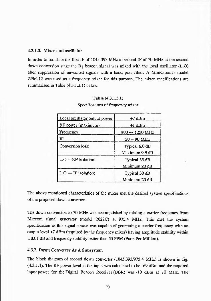
4.3.1.3. Mixer and oscillator

In order to translate the first IF of 1045.393 MHz to second IF of 70 MHz at the second down conversion stage the beacon signal was mixed with the local oscillator (L.O) after suppression of unwanted signals with a band pass filter. A MiniCircuit's model ZFM-12 was used as a frequency mixer for this purpose. The mixer specifications are summarised in Table (4.3.1.3.1) below:

Table (4.3.1.3.1) Specifications of frequency mixer.

Local oscillator output power +7 dBmRF power (maximum) +1 dBmFrequency 800 — 1250 MHzIF 50 - 90 MHzConversion loss: Typical 6.0 dB j

Maximum 9.5 dB (L.O —RF isolation: Typical 35 dB |

Minimum 20 dB \L .0 — IF isolation: Typical 30 dB |

Minimum 20 dB \

The above mentioned characteristics of the mixer met the desired system specifications of the proposed down converter.

The down conversion to 70 MHz was accomplished by mixing a carrier frequency from Marconi signal generator (model 2022C) at 975.4 MHz. This met the system specification as this signal source was capable of generating a carrier frequency with an output level +7 dBm (required by the frequency mixer) having amplitude stability within ±0.01 dB and frequency stability better than 55 PPM (Parts Per Million).

4.3.2. Down Converter As A Subsystem

The block diagram of second down converter (1045.393/975.4 MHz) is shown in fig.(4.3.1.1). The RF power level at the input was calculated to be -69 dBm and the required input power for the Digital Beacon Receiver (DBR) w as-10 dBm at 70 MHz. The

70

down conversion of Bj signal 1.045 GHz to 70 MHz was done in one stage while the required amplification was achieved at two different frequencies.

At point A in fig. (4.3.1.1) there were other undesired signals emerging after down conversion by the first down converter (19770.393/18725 MHz), located outdoor by the antenna. These undesired signals were suppressed by the band pass filter. The Band Pass Filter (BPF) offered 2.2 dB insertion loss at centre frequency, f0= 1.045 GHz. The use of this BPF not only filtered the unwanted signals but also protected the first amplifier from saturation. The beacon signal was amplified around 1 GHz between point B and C and in the following stage was mixed with 975.4 MHz from the local oscillator for down conversion to 70 MHz . A low pass filter was introduced between point D and E at the second IF to remove the undesired high frequency signals arriving from the local oscillator. The reason for implementation of the low pass filter before the final amplification was to protect the 70 MHz amplifier from saturation when operating between points E and F. Finally the beacon signal was interfaced to the DBR through an adjustable attenuator with a flexible 50 ohms coaxial cable.

The second down converter which acts as a subsystem in the whole beacon transmission reception chain (presently only for single polarisation) was placed in a temperature controlled unit, like the first down converter, to minimise equipment performance variation due to temperature changes.

The development of the down converter was necessary as part of the radio wave propagation study at ka frequency band making use of the front end of the CODE terminal. The complete experimental arrangement is shown in fig. (4.3.2.1). The developed part of second down converter is marked with dashed lines.

4,4, BEACON RECEIVER AND TEST PERFORMANCE

In conventional high performance satellite beacon receivers the tracking circuits are based around Phase Lock Loops (PLL) with bandwidths of few tens of Hz. On occurrence of the most interesting propagation events, for example very deep fades, the performance of a PLL receiver degrades drastically due to its inherent carrier/noise density threshold. Moreover, as the propagation path recovers, the PLL has to either re­acquire the signal or to have previously stored parameters of the unfaded signal as an aid to reacquisition [Ransome, 1990], The loop bandwidth of the PLL is typically 50 Hz,

71

giving a carrier/noise density (C/N0) tracking threshold of 25 to 30 dB Hz [DBR1-S Manual, 1991].

The DBR1-S (Digital Beacon Receiver for Switched beacon B^) developed by Signal Processors Ltd. was designed to overcome the above mentioned problem in addition to maintaining lock down to a point 15 dB below the typical C/N0 limit for a PLL. This was achieved by the elimination of feedback loops with a feed forward architecture. Digital processing implies stability, accuracy and repeatability. The tracking of the beacon carrier is achieved by tracking the carrier frequency independently of its phase. Instead of PLL, the carrier frequency tracking is performed by a digital Fourier transform processor, with a bin bandwidth of approximately 2 Hz. As the beacon signal fades, accuracy degrades gracefully, and is restored immediately on signal recovery, even if the signal has faded into noise (i.e. loss of lock).

Benefits of this digital processing approach include the minimisation of operator adjustments, stability of measuring circuit with time and repeatability. In the following Table (4.4.1) performance specifications are summarised [DBR1-S Manual, 1991; Ransome, 1990].

Table (4.4.1)Beacon receiver performance specifications.

Nominal input frequency 70 MHz

Receiver bandwidth ±400 KHzNoise figure -16 dBInput power level -10 dBmC/Nn Dynamic range limits 69 dB Hz (over load)Carrier acquisition level 41 dB Hz C/Nn± 2 ° Phase accuracy point 30 dB Hz C/NnCarrier phase measurement threshold 23dB H zC /N nCarrier frequency tracking threshold 9 dB Hz C/NnOutput signals HHI HHQ

VHI VHQ

Output sample rate 99.96 HzOperating temperature 0 - 40°C

72

The beacon measurement reliability of the receiver was quantified by carrying out a linearity test. The test procedures are given [Ransome, 1989] below as:

A CW signal at 70 MHz, -10 dBm total power (66 dB Hz C/N0), was applied through a 50 O coaxial cable. DBR1-S was reset via the front panel. When "carrier frequency" and "carrier phase" were locked the signal level was decreased in steps of 1 dB to -46 dB (30 dB Hz C/N0). For each step the PC display of power was recorded. The mean displayed figure was found within 0.2 dB. The results are summarised in Table (4.4.2) below:

Table (4.4.2)Linearity test results of the beacon receiver.

Signal power (dBm) PC display (dBm) Error (dB)

-10 -9.87 0.13-11 -10.85 0.15 |-12 -11.84 0.16 |-13 -12.82 0.18 j

-14 -13.80 0.20-15 -14.82 0.18 !-16 -15.80 0.20 |-17 -16.81 0.19 j-18 -17.80 0.20-19 -18.87 0.13

■ to O -19.83 0.17-21 -20.84 0.16-23 -22.83 0.17-24 -23.80 0.20-25 -24.80 0.20-26 -25.80 0.20-27 -26.80 0.20-28 -27.80 0.20-29 -28.97 0.03

73

Table (4.4.2). Continued

Signal power (dBm) PC display (dBm) Error (dB)

-30 -29.90 0.10

-31 -30.90 0.10-32 -31.94 0.06-33 -32.88 0.12-34 -33.93 0.07-35 -34.87 0.13-36 -35.92 0.08

-37 -36.90 0.10-38 -37.90 0.10-39 -38.90 0.10-40 39.80 0.20-41 -40.87 0,13-42 -41.89 0.11-43 -42.86 0.14-44 -43.82 0.18-45 I 00 u> U* 1 /

4,5, WEATHER STATION

The impairments introduced by atmospheric turbulence to radio wave signals could be correlated by operating a weather station in the vicinity of the radio wave measurement site. Therefore, a weather station was installed to observe the effects of rain on radio wave signals transmitted from Olympus at 20 GHz.

A Personal Computer Weather (PCW) station was installed as a part of the equipment used in this project. This small unit plugs into the expansion slot of an IBM compatible PC. It was interfaced to a PC (ISIS 400), as shown in fig. (4.5.1). This weather station is composed of the followings units:

© Rain collector, RG-2.® Two temperature sensors; temperature A and temperature B.© Anemometer.

74

® Weather station interfacing card to PC.

(a). Rain collectorThe RG-2 rain collector is a syphon rainguage. In this type of rainguage the water is funnelled to a special reservoir containing a measuring device, such as a floater, to continuously measure the total volume of the received water.

The RG-2 unit measured rain with a resolution of 1/10 inch (approx. 2.5 mm) with good accuracy. The water is funnelled to a small reservoir which contained a special floating device. When this reservoir collected a measurable quantity of water, the unit recorded the quantity and then drained the water out.

(b). Temperature sensorsTwo temperature probes were also included in the PCW weather station. These two temperature sensors could be used to measure the outdoor temperature A and the indoor temperature B with a resolution of ±0.1° C.

(c). AnemometerThe anemometer included in the weather station measured wind speed and direction with high accuracy. Note that the wind speed and direction generally has only a limited effect on the radio wave signal for satellite communication. So the effects of gust were not incorporated in this study of radio wave propagation.

(d). Weather station interfacing card to PCA half slot PC board interfacing card with weather data acquisition software was also available with the PCW station. The interfacing card was set on port address 300 hex. by the manufacturer. Modification in the hardware was made to change the port address to 340 hex. since there was already another card used by another user with the 300 hex. port address. The hardware port selection changes are outlined in appendix (II).

4.5.1. Data Logging And Display

The PCW station also included data acquisition software called PCW. The weather data can be acquired either in the foreground or background mode. The background data acquisition mode was preferred due to the following reasons:

(i). Data backup was done without loss of any event.

75

(ii). In the foreground the modified program (MPCW) remained in operation.

In the background (RAM resident) mode the software, PCW, updated the registers present in the weather station data collection hardware for each interval of one minute. Whereas, in the foreground mode, the PCW displayed the instantaneous weather changes on the PC screen. However, in either of these two modes, the PCW stored the weather information in a data file every half an hour.

In the RAM resident mode, the current weather status could be visualised by pressing a user defined key. The PCW software provides a graphical presentations of weather events such as rainfall, temperature and wind in a weather bulletin on the screen. The PCW also allows to plot the current data together with the previous day's data at the same time on the screen. The data was stored in the ASCII format.

4.5.2. An Adaptive Time Based Technique To Determine Rain Rate

The rain rate measurement is an inexact process because of the discrete nature of rainfall [Ippolito, 1989]. The rain rate is computed by measuring the rain accumulation per given area for a known period of time at a given point.

There were two problems associated with the PCW weather station:

(i). The rain gauge, RG -2, available with the weather station had a resolution of 0.1 inch or 2.5 mm, which limited the measurement of light rain events.

(ii). The data acquisition software, PCW, had the data logging interval of half an hour. The same interval time, eventually, would have been used for the integration purpose to calculate the rain rate.

Suppose that there was a heavy burst of rain for sufficient length of time to measure 2.5 mm rain. This would be recorded after 30 min. in RAM resident mode. In the foreground mode it would be displayed instantaneously on the screen but would be stored on the hard disk in a data file after 30 minutes. If there was another burst of rain in the same 30 minute interval, than the measurement of the two rain events would have not been independent. Therefore, the correlation between the particular rain events and the

76

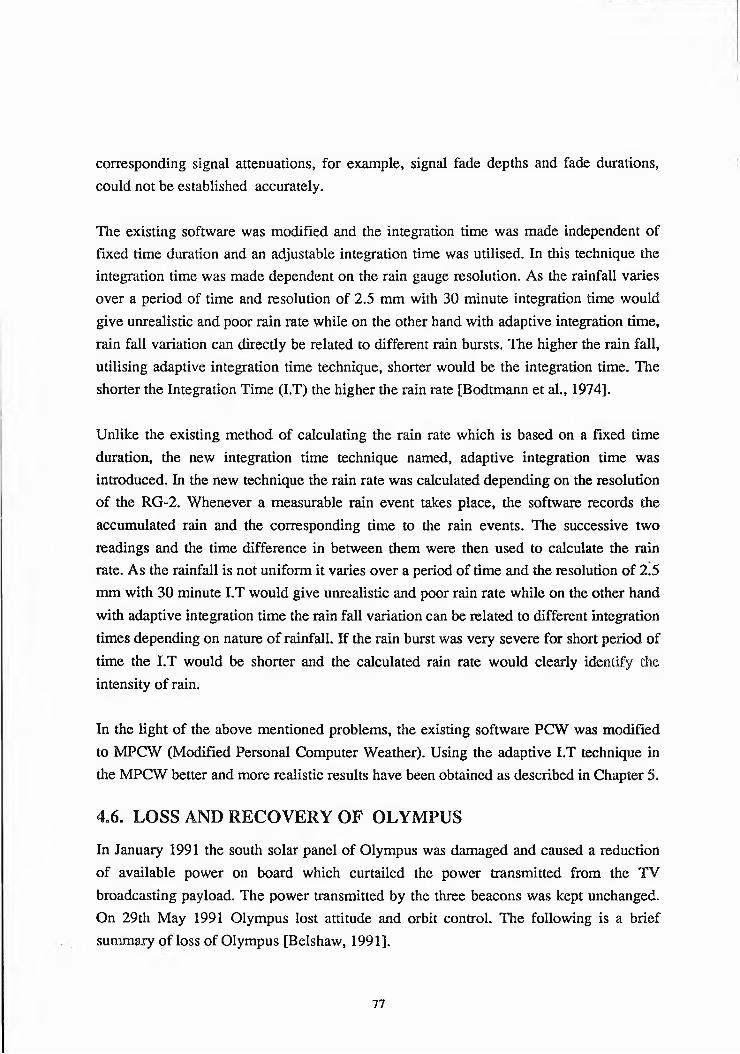
corresponding signal attenuations, for example, signal fade depths and fade durations, could not be established accurately.

The existing software was modified and the integration time was made independent of fixed time duration and an adjustable integration time was utilised. In this technique the integration time was made dependent on the rain gauge resolution. As the rainfall varies over a period of time and resolution of 2.5 mm with 30 minute integration time would give unrealistic and poor rain rate while on the other hand with adaptive integration time, rain fall variation can directly be related to different rain bursts. The higher the rain fall, utilising adaptive integration time technique, shorter would be the integration time. The shorter the Integration Time (I.T) the higher the rain rate [Bodtmann et al., 1974].

Unlike the existing method of calculating the rain rate which is based on a fixed time duration, the new integration time technique named, adaptive integration time was introduced. In the new technique the rain rate was calculated depending on the resolution of the RG-2. Whenever a measurable rain event takes place, the software records the accumulated rain and the corresponding time to the rain events. The successive two readings and the time difference in between them were then used to calculate the rain rate. As the rainfall is not uniform it varies over a period of time and the resolution of 2.5 mm with 30 minute I.T would give unrealistic and poor rain rate while on the other hand with adaptive integration time the rain fall variation can be related to different integration times depending on nature of rainfall. If the rain burst was very severe for short period of time the I.T would be shorter and the calculated rain rate would clearly identify die intensity of rain.

In the light of the above mentioned problems, the existing software PCW was modified to MPCW (Modified Personal Computer Weather). Using the adaptive I.T technique in the MPCW better and more realistic results have been obtained as described in Chapter 5.

4,6, LOSS AND RECOVERY OF OLYMPUS

In January 1991 the south solar panel of Olympus was damaged and caused a reduction of available power on board which curtailed the power transmitted from the TV broadcasting payload. The power transmitted by the three beacons was kept unchanged. On 29th May 1991 Olympus lost attitude and orbit control. The following is a brief summary of loss of Olympus [Belshaw, 1991].

77

Some time before its loss, British Aerospace introduced a new attitude control software. It was designed, specially, to save some fuel and extend the satellite life time. This software caused contradictory telemetry to be transmitted by the satellite. Meanwhile an urgent resumption of earth pointing was required owing to a high definition television demonstration. The repointing manoeuvre was undertaken, but something, caused a loss of satellite control.

The result of this anomalous satellite manoeuvre was that a thruster was fired for 28 minutes (used approximately 6 months fuel supply) and caused the satellite to spin in the x-axis, with the solar array edgeways to the sun. The spin rate was 90 seconds per revolution with an orbital drift of 5° per day towards East. The temperature fell to a very low level (-60° C) and telemetry was only sent once per revolution when the arrays received enough power.

By June 1991 Olympus had drifted around the geostationary orbit to a position giving better solar illumination and the command station was able to receive continuous telemetry and diagnose the satellite status. Olympus responded to the control commands and the power system was heated and the batteries were slowly charged to 25 % capacity. On 1st July 1991 the working solar panel was rotated to improve the sun angle which resulted in power increase of 1.6 Kilo Watts. By 3rd July the batteries were fully charged and 100 W of heater power was switched in an attempt to defrost the fuel system. The Hydrazine propellant forms a slush when frozen and expands on melting. Hence the fuel was slowly defrosted to allow expansion into empty tanks and prevent burst pipe. This had never been done before; fortunately, the critical stage was successfully completed.

The optimistic hopes of Olympus recovery were justified and finally it was restored and recommissioned on 14th August 1991. It resumed its beacon transmission, after an absence of about three months, on 16th August, The amplitude stability of the beacon was not as good as before. A cyclic variation of up to 4 dB peak to peak was observed at the University of Surrey site. This diurnal amplitude variation could limit the validity of statistical analysis, however, with data pre-processing software more meaningful results were obtained.

78

4.7. M AYAK AS AN ALTERNATIVE SATELLITE

In the absence of Olympus other satellites such as DFS-Kopemicus, Italsat and MAYAK were considered. A comparison table between these satellites [Jeay, 1991] showed that reception of MAYAK beacon transmission was possible. MAYAK was the only one that allowed meaningful fade measurements.

The beacon data acquisition software, written in "C language" [Jeay, 1991] was under development at time of the Olympus disappearance. Nevertheless the software was developed for the Olympus beacon B j and slightly modified later for the MAYAK beacon and few events were recorded which are also presented in chapter 5.

The MAYAK was located at 14° W in geostationary orbit and was transmitting three beacon signals at 11.542 GHz, 19.237 GHz and 28.856 GHz with EIRP of 20 dB W each which was 12 dB down compared to Olympus beacon B k The coverage area of the circularly polarised beacon signal at 19.237 GHz is shown in fig. (4.7.1). As mentioned earlier in section (4.3) that with the present system configuration only horizontally polarised transmission could be received. Tire reception of circularly polarised signal would mean loss of 3 dB in received signal power level. However the necessary modifications were made at the second down converter after the calculation of link budget for MAYAK measurements. The link budget for MAYAK is presented in the following Table (4.7.1).

79

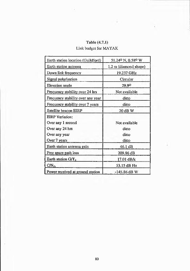
Table (4.7.1)Link budget for MAYAK

Earth station location (Guildford) 51.24° N, 0.58° WEarth station antenna 1.2 m (diamond shape)Down link frequency 19.237 GHzSignal polarisation CircularElevation angle 29.9°Frequency stability over 24 hrs Not availableFrequency stability over any year dittoFrequency stability over 7 years dittoSatellite beacon EIRP 20 dB WEIRP Variation: Over any 1 second Over any 24 hrs Over any year Over 7 years

Not available ditto ditto ditto

Earth station antenna gain 46.1 dBFree space path loss 209.86 dBEarth station G/TQ 17.01 dB/k

C/Nn 53.15 dB HzPower received at ground station “145.86 dB W

80

(T

03 co

mP

§

o

sz;o

Q

O

< dPmZOucw£Q

t\j CDJ:kVQohv.vooqouocm

CD4—> C—03 CD

C/0• o

OC/0

C l

E<

CMX

<_o

4—>03 CO4-J 1—-CO 'X CJc_ 03

(_ ) o

3 :£xLON -cdxr><;vo

CO<_CD

Q .

<

Nl

ILO05iniriinvo05CM

(NCD

A

K )X

X COCJc

c_CD

K ) CD ,— ^ rT -sgg— ■ 3 C l —— K)

X CTCD 4—> Xt_Ll_ 3

7 "

"Oc3_o■>,03CXCo8<DCQ00acxE

bb•S3•a

83<

1boE

\x__

81

82

83

84

B a n d p a s s F i l t e r R e s p o n s e

F r e q u e n c y (M H z )

Figure (4.3.1.1.1). Frequency response of bandpass filter.

BW Vs IL

Figure (4.3.1.1.2). A graphical presentation of bandwidth response.

85

FR E Q U E N C Y R ESPO N SE O F LO W PASS F IL T E R

F re q u e n c y (M H z)

Figure (4.3.1.1.3). A graphical presentation of Iowpass filter response.

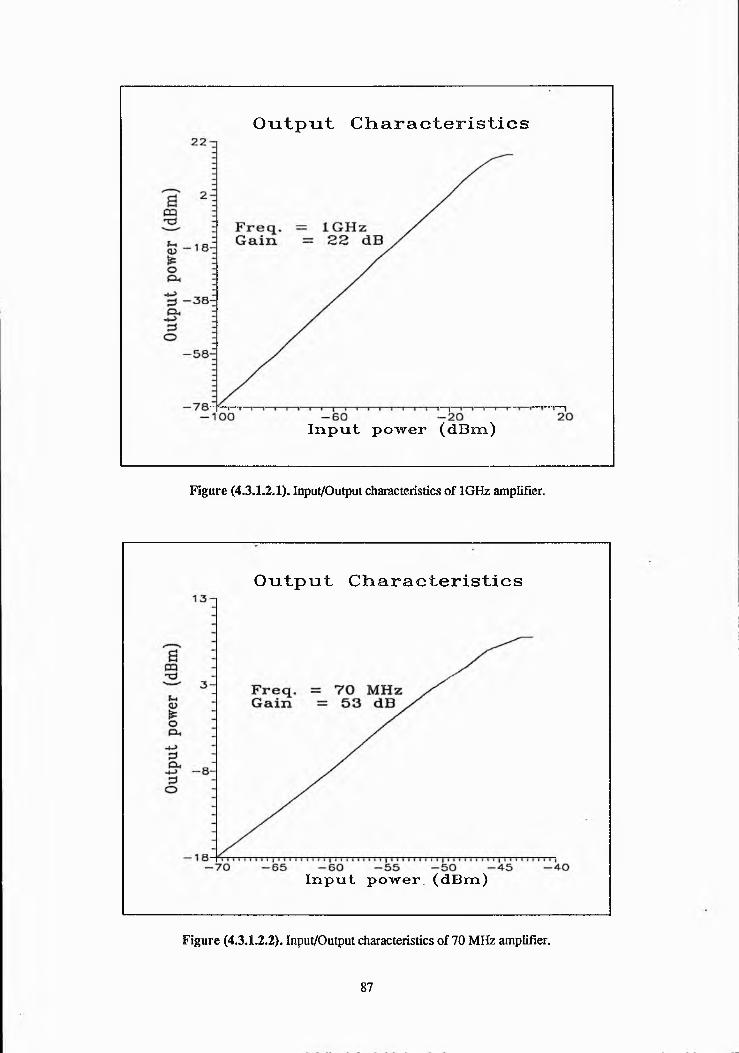
O u t p u t C h a r a c t e r i s t i c s

I n p u t p o w e r ( d B m )

Figure (4.3.1.2.X). Input/Output characteristics of 1GHz amplifier.

O u t p u t C h a r a c t e r i s t i c s

I n p u t power . ( d B m )

Figure (4.3.1.2.2). Input/Output characteristics of 70 MHz amplifier.

87

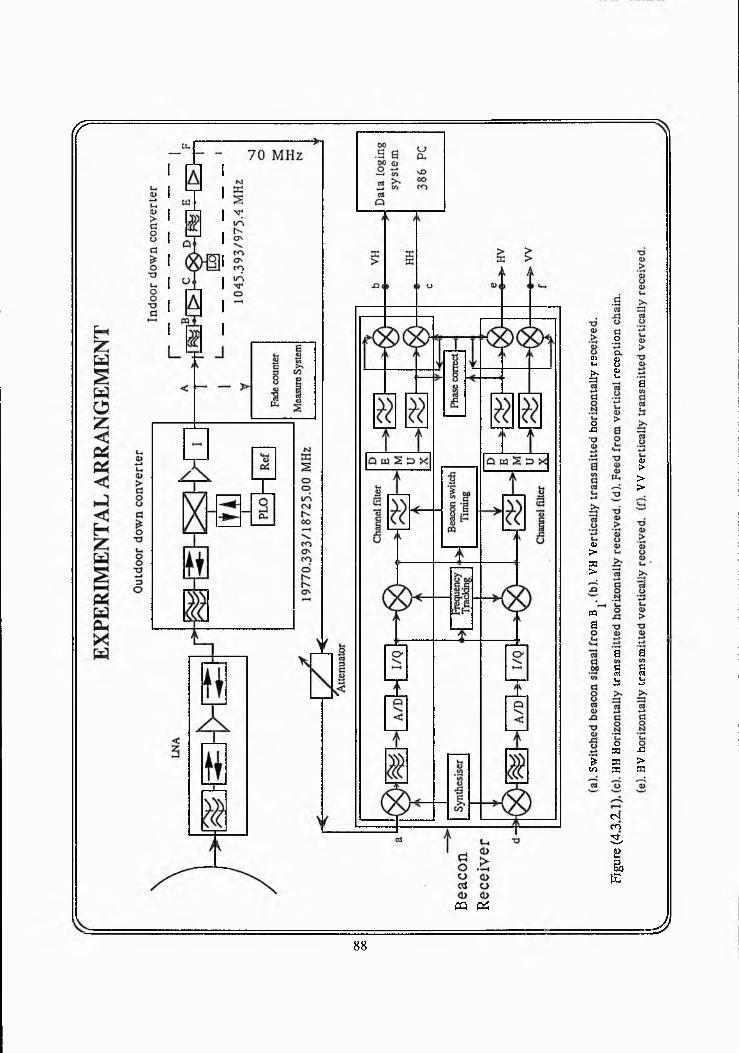
< r

PQ Pi

oQ> Q>l* oi- t

oXI

Q>>ft>

PQ

a

*V)

a

a>>>>

a ae gra rais is

oft33ft

CScnS¥S)E

ft>ft

A 188

*\

CS.2 •s—Iod

u,<D"3ed<D£

OC/3 +~» • *—Nc BuOo“O<—>3O

t=<ooX3.aocso

• a5CS<l>C/32p ,

38<DJ3O

^ 2

iqs£¥3W>• «=*=*tL,

89

CHAPTER 5

RESULTS OF MEASUREMENTS TAKEN USING ka BAND BEACONS

Olympus was launched by an Ariane vehicle on 12th July 1989. Its geostationary orbital position is 19° West. It has been maintained in an operational state for two years until, on 29th May 1991, the satellite was manoeuvred into an uncontrollable position. It has been restored and recommissioned on 14th August 1991. Olympus beacon at 19.77 GHz was continued to be measured after its recovery. In its absence ka beacon transmission from the Russian satellite MAYAK was measured at 19.23 GHz. In this chapter some of the measurements taken using ka band beacons are presented. Data analysis of few significant events were carried out. Although the objective of this work was to study the Olympus beacon B j, however, the experimental arrangement was altered for MAYAK beacon due to the problems with Olympus. Later on the Olympus was restored and once again the experimental arrangement was modified.

5.1. OLYM PUS B i DATA COLLECTION.

The beacon package on board the Olympus is providing a unique opportunity to carry out long term statistical evaluation of radio wave propagation at 12.5, 20 and 30 GHz. In Europe before Olympus satellite, beacon measurements were taken using ATS-6 satellite in ka frequency band during 1975-76. The available data [ATS-6, 1977] was recorded over a short period of time. In addition, 1975-76 was a year with low average rainfall and therefore is not a true representative of a typical year. During the Olympus measurement campaign, a large amount of data will be collected by experimenters at different locations. This long term measured propagation data may then be utilised for the performance evaluation of existing models. In addition, more regional rain attenuation prediction models can be developed on the basis of the measurements which will be useful in designing future satellite communication links above 10 GHz.

The three beacon signals were again available after the restoration of Olympus in August 1991. Experimental arrangements for radio wave propagation study using Olympus beacon ®i has been established. The campaign of long term data collection, using Olympus, has been started at Guildford earth station since 20th August 1991. The

91

measured rain attenuation data set at Guildford along with other OPEX members can be incorporated in the existing data in Europe.

5.2. B i DATA PRE-PROCESSING

Data pre-processing is an essential part to be carried out before data analysis as the raw data usually contains unwanted information, in some cases, redundant information. Therefore the duplicate information should be eliminated from the original data file in order to produce more reliable results.

Although, Olympus was retrieved and the beacon payload is transmitting three signals at specified power levels, the performance of Olympus has not been as good as before the loss of the satellite. A regular station keeping (±0.07° N/S and E/W) was carried out before the loss of the satellite. After the recovery the station keeping has been relaxed to 0.1° N/S [Belshaw, 1992] which is 1.4 times worse than before. A peak to peak cyclic variation of up to 4 dB has been observed in the received beacon signal over 24 hours, as shown fig. (5.2.2). The cyclic variation in the MAYAK beacon transmission was many times higher than the Olympus. The station keeping for MAYAK was ± 2 ° N/S [Jeay,1991]. The maximum variation of upto 18 dB has been recorded, as shown in fig. (5.2.1). This undesired variation of the beacon transmissions for propagation measurements can be compensated in the data pre-processing software.

The option of software compensation of diurnal variation of the beacons signal has been utilised at the pre-processing stage. Several programmes have been written in computer language C which were used for the elimination of the unwanted cyclic variations of the Olympus and the MAYAK beacon transmissions (data pre-processing programmes are given in appendix IV).

The cyclic variations of the beacons have been compensated by taking the average diurnal variation of several dry days as a mean daily variation. The average variation was then subtracted from the data files which contained significant attenuation events. Typical sunny day's beacon signal variation of the Russian satellite MAYAK and the Olympus is shown in fig. (5.2.1) and (5.2.2), respectively.

92

5.3. B i DATA PRESENTATION

The measured propagation data can be presented in many ways. One of the ways is via diurnal variation and monthly statistics [Ippolito, 1989]. CCIR report [CCIR Rep. 564- 4,1990] outlines the cumulative distribution presentation. Some ways of data presentation in tabular and graphical form are also given in [Larsen, 1991]. For graphical presentation Quattro Pro software was used.

For Olympus propagation data analysis a software called DAPPER (Data Analysis and Pre-Processing Effects Research) has been developed. This is the standard form of data analysis and presentation agreed by all OPEX members. Unfortunately, the DAPPER analysis package could not be used for the initially recorded data due to the fact that the captured raw data files were not compatible with the DAPPER format. The Quattro Pro was not available as well, therefore, other software packages such as Matlab and Grapher has been used for Olympus beacon B \ and MAYAK data presentation.

The above mentioned packages have limitations in terms of data points, therefore, for some analysis only the more interesting events were selected. Two methods of rain attenuation data presentation were adopted :

(a). Time plot

These type of graphs are very useful in understanding the general behaviour of the received signal and in identifying the number of events in a day. Furthermore, the start and the end time of events can also be calculated from these kind of graphs. One minute averaging has been chosen for the following reasons:

© Acceptable to all OPEX members.© The accepted way of attenuation data presentation is 1 min average [Rucker, 1991],

as defined by the CCIR.® Limitations of software package. The Matlab/Grapher is restricted to limited number

of input data points, i.e, 8192 elements or 4096 vectors. This means twenty four hours data with 10 second averaging could not be presented.

93

The time plot graphical presentation of preliminary recorded data using the Olympus and the MAYAK beacons have been presented in fig. (5.3.1) through (5.3.14). Some expanded views of events are also given.

(b). Histograms

This is a conventional way of presenting statistical data. Presentation of this kind is more useful than a time plot due to the fact that only the wanted events are generally selected which yields the basic information about the signal fluctuation and fade depth.

The data acquisition software has employed a wait state [Jeay, 1991]. If the attenuation level is below certain threshold level, presently 0.1 dB, the acquisition software waits until 10 seconds before storing the attenuation value and the corresponding time. However, during fade events the attenuation level and the corresponding time is recorded every second. Histograms of all events presented are given, in fig. (5.3.16) through (5.3.22), and a 10 seconds time averaging has been taken since the acquisition software has a waiting time of 10 seconds.

5 .4 B i DATA ANALYSIS

The aim of the OPEX group is to aggregate the propagation data of individual ground stations into a large common data base. Project COST 205 has the same objectives and has shown that propagation data of different sources forming input for the data base must be of high quality. Moreover, the data should be comparable and compatible [CCIR Rep. 564-4, 1990]. Therefore standardisation of procedures for the data treatment performed by individual experimenters operating different ground stations is important.

The main objective of standardised data pre-processing is to achieve more reliable data ready for scientific analysis between different users or suitable for a centralised data bank. Data analysis and pre-processing package DAPPER is a suitable package for this purpose. However, this package could not be used at this stage as mentioned earlier.

Other standard analysis methods were investigated. Several analysis programmes were written (see appendix IV) which were used in conjunction with Matlab for data analysis of preliminary recorded propagation events.

94

5.4.1. Fade Duration

In satellite communication systems the maintenance of a fixed large fade margin to overcome, occasional deep fades, may result in an excessive satellite power. This large satellite power will not be required for a large percentage (e.g 99%) of the time. An effective method to overcome this problem is the dynamic power control technique [Lin et al., 1980]. In this approach a small fade margin of the radio link is increased during heavy rain periods by increasing the transmitted power. The increased transmitter power on board the satellite during rain is supported by batteries which are usually provided to cover the eclipse periods. However, prolonged and repeated use of these batteries during heavy rain period may exhaust the battery capacity and result in an outage.

In addition to fade depth, fade slope and duration were considered to be two of the key parameters in an adaptive power control system [Dintelmann, 1981]. The statistics of duration of rain attenuation fade are, therefore, important in the optimal design of a dynamic power control system involving trade-offs between battery size, fade margin, transmission capacity and satellite cost etc.

Investigations into the duration of fades have been made at several locations, frequencies and elevations. Unfortunately, very few statistical data are available [CCIR Rep. 564-4, 1990] according to which duration of fades exceeding certain levels seem to have a log­normal distribution [Dintelmann, 1981; Lin et al., 1980] with median values of the order of several minutes. For fade levels of less than 20 dB, no significant dependence of these distributions on the fade level is evident from the measurements. This would mean that the large total time percentage of fades observed e.g for lower fade levels are made up from a large number of individual fades having more or less the same distribution of durations. However, measurements taken in 1985 during the COST 205 project suggest significant departures from a log-normal distribution for fade duration less than about half a minute [CCIR Rep. 564-4, 1990].

Fading durations have been obtained experimentally in ka band using satellite beacons such as ATS-6 and ETS-II. The ATS-6 measurements in England are summarised in a review of the slant path work at Slough by Davies and Mackenzie [1981]. The ETS-II measurements carried out by Japanese researchers are described in a NASA publication flppolito, 1989].

95

Fade duration distributions can be presented in many ways and these are well described in [Lin, 1980; Dintelmann, 1981; Ippolito, 1989; CCIR Rep. 564-4, 1990]. In this thesis the CCIR method of presentation is adopted as it is well accepted world wide. Fade duration distribution of the MAYAK and the Olympus beacons have been presented in fig. (5.4.1.1) through (5.4.1.7). Event based cumulative fade duration distribution for the Olympus beacon is shown in fig. (5.4.1.7). The overall fade duration distribution, given in fig. (5.4.1.8), has been obtained by incorporating the data collected using the MAYAK beacon.

The limited rain attenuation data recorded at Guildford, in the first two months after the restoration of the Olympus, has been analysed for cumulative fade interval distribution. Fade interval or fade frequency analysis has been documented, from January to March 1990, using data from the Swedish/Danish Olympus measurements for 1, 2, 3 and 5 dB fade levels in [Larsen, 1991]; 7 dB fade occurrence reported only once. A software package called Quattro Pro was used for graphical presentation of cumulative interval distribution. As described earlier this software package was not available. However, for the sake of comparison the 50% or median durations for the four attenuation levels with the corresponding mean durations are given in Table (5.4.1.1). Only events >2 seconds were considered.

Table (5.4.1.1). Statistics on fade duration, based on number of events.

j Swedis h/Danish measurements Guildford MeasurementsAttenuation level (dB)

Median fade duration (Sec.)

Mean fade duration (Sec.)

Median fade duration (Sec.)

Mean fade duration (Sec.)

1 4.5 47.8 2.3 54.02 4.5 27.4 15.3 50.93 5.0 19.4 7.3 29.55 9.0 27.5 9.0 42.0

5.4.2. Rate Of Change Of Attenuation

In future satellite communications systems uplink power control can be employed to reduce link degradation by monitoring down link signals and predicting appropriate counter measures. The systems should be designed such that situations of deep fade, for which normal resoarcss^^srteu^cient*- will take place within. .the time required to

96

switch from one system configuration to another suited to meet the new demand. This calls for information on the rate of change of the rain induced attenuation, which in turn depends on the attenuation level [Matricciani, 1981].

In practice, the electric field strength observed on the down link may fluctuate around a certain fade threshold, which would cause frequent power switching. Therefore if the decision when to increase or to decrease the uplink power were based on the fade level alone, this would result in a poor system performance [Dintelmann, 1981]. Monitoring the fade slope is considered to improve the decision making process by providing information on the rate of change of signal amplitude and possibly enabling forward predictions to be made.

Within the frame work of the OTS propagation experiments, fade slope data at 11.8 GHz were analysed at a fade level of 5 dB [Dintelmann, 1981]. Fade slopes were found to be log-normally distributed and the distribution was symmetric for the starting slopes and the ending slopes with a median value of 0.12 dB/s. Similar results were obtained for various fade levels in America using CTS 11.7 GHz beacon [CCIR Rep. 564-4, 1990]. The fade slope was found to be only slightly dependent on fade level. Observation made at a frequency of 11.6 GHz using SIRIO in Italy [Matricciani', 1981] have shown th a t:

© The higher the attenuation, the higher the rate of change of attenuation.© Positive and negative rates of change have very similar distributions.© The distribution function is not affected by assuming different values of the

separation between successive attenuations used to determine the rate of change.

There is broad agreement that distribution of positive and negative slopes are log-normal and very similar to each other.

5.5. PERCEN T OF TIM E PERFORM ANCEIt is often necessary and advantageous to specify certain communications link system

parameters on a statistical basis. This is particularly required when considering parameters affected by propagation factors, since the basic propagation mechanism are not deterministic and can only be described on a statistical basis [Ippolito, 1986].

97

Statistically based performance parameters are usually specified on a percent of time basis that is the percentage of time in a year, or a month, that the parameter is equal or exceeds a specific value. In this thesis so far event based analysis has been presented, therefore percent of event time attenuation exceeded ordinate is shown in fig. (5.5.1) for 1st August, 1991. Two day's data were combined for better result, as shown in fig.(5.5.4) and (5.5.5). Figure (5.5.6) represents cumulative distribution of all events recorded using the Olympus beacon and the fig. (5.5.7) gives the over all cumulative distribution obtained by incorporating the measurements taken from the MAYAK beacon.

5.6. EXPERIM ENTAL RESULTS AND DISCUSSIONBeacon measurements are in progress since the return of Olympus. The weather station was not operational until 25th July 1991. Some preliminary recorded propagation events and corresponding rain are presented in this chapter. In the absence of the Olympus ka band beacon, measurement was continued using the Russian satellite, MAYAK. A peak to peak variation of several decibels was observed in the MAYAK beacon transmissions as shown in fig. (5.2.1). Such large daily variations can make any statistical analysis of this data invalid from a systems design engineers point of view.

The data recorded from the MAYAK beacon has large cyclic variation which has been removed at the data pre-processing stage. Few propagation events recorded using MAYAK are also presented in the thesis. A limited data was collected from MAYAK because of two reasons. Firstly, the data acquisition software was under development [Jeay, 1991]. Secondly, the Olympus was restored in mid August, 1991 and ka band data collection campaign continued using ESA's satellite.

The beacon receiver, DBR1-S, could measure signal fade depth up to 35 dB [DBRl-S Manual, 1991]. In the case of the MAYAK beacon it is interesting to observe, in the early twelve hours of the day, the dynamic range of the DBRl-S. In the first half of the day the effective dynamic range was limited to 17 dB because of the peak variation of as high as 18 dB. During the peak variation (at 6:30) the fluctuation rate was low but on either sides of the peak the variation rate was high; nevertheless, on either sides the effective dynamic range of the beacon receiver was better than 17 dB. Although the cyclic variation can be eliminated in the pre-processing software doubt remains in the

98

pure fade depth in case when the signal fade is greater than the dynamic range of DBR1-S.

The beacon receiver can measure a maximum fade step of 5 dB [Ransome, 1989] which means that any abrupt fade depth of greater than 5 dB will result in loss of lock. Now consider fig. (5.3.1), unfortunately, the weather data was not available but some event in conjunction with the cyclic variation must have caused signal attenuation in step of greater than 5 dB which resulted in loss of lock. The loss of lock effect can be seen from fig. (5.3.1a) and (5.3.1b). This is the reason the 4th July's data has not been processed any further. On the other hand data of 1st August, after the eradication, has been incorporated in the cumulative distributions, as shown in fig. (5.4.1.8) and (5.5.7). Event based analysis of 1st August has also been done. Figure (5.4.1.1) shows fade duration distribution which reveals that 5, 10, 20 and 35 dB fade lasted about 15, 9, 6 and 5 minutes, respectively. The maximum positive fade rate, defined as the maximum attenuation difference between two fade levels, was 4.65 dB/sec and the maximum recovery or negative fade rate was 3.18 dB/sec. Figure (5.5.1) is the percent of event time presentation of 1st August which reveals that 2% of event time the fade level was greater than 35 dB while 50% the fade level was higher than 1 dB and 100% of the event time the fade level was above 0.5 dB.

Similar, analysis has been carried out for the data recorded after the recovery of Olympus. In the case of Olympus, relatively, better and wider data set was obtained. As mentioned earlier Olympus beacon Bj exhibited a maximum peak to peak variation of 4 dB. This unwanted non atmospheric fluctuation has been eliminated by the pre­processing software. Fade duration distribution of 22nd August is given in fig. (5.4.1.2) which shows that the signal remained in fade depth of 5 and 10 dB for about 11 and 5 minutes, respectively. The maximum positive fade rate was 0.96 dB/sec while the maximum negative fade rate observed as 0.88 dB/sec. Figure (5.5.2) is the percent of event time presentation of 22nd August.

Now consider Figure (5.3.8) and (5.3.9) which are time plot of 23rd August beacon data and corresponding rain events, respectvely. A good correlation exits between the recorded signal attenuation and the rain rate. On the 23rd August the rain started around 11:30 and after mid day it intensified gradually. At 13:57 it became a heavy thunder storm which resulted in a very deep fade. As described in the previous chapter that the rain gauge was a slow rain gauge with 2.54 mm resolution. Furthermore, the data logging

99

interval of weather data acquisition software (PCW) was thirty minutes. This time, eventually, was utilised for the computation of rain rate, which turned out to be 18 mm/hr as shown in fig. (5.3.9). The modified weather data acquisition software (MPCW) has overcome the delayed storing but it cannot cure the deficiency of the rain gauge resolution. However, with the new integration time technique termed as "adaptive integration time" the same rain events were calculated in terms of rain rate as 76 mm/hr and is shown in fig. (5.3.9).

The rain attenuation models predictions (see chapter 3) were used for the verification of this technique by comparing the rain rate and the corresponding fade depth. The CCIR rain attenuation prediction corresponding to 76 mm/hr was grater than 35 dB. The Crane rain attenuation prediction for the same rain rate was even higher than CCIR, SAM and Lin rain attenuation prediction for the above mentioned rain rate was more than 36 and 45 dB, respectively. On the other hand, all models predicted fade depth corresponding to rain rate of 18 mm/hr was less than 15 dB.

Fade duration distribution curve for 22nd and 23rd August is shown in fig. (5 A 1.2) and(5.4.1.3), respectively. Figure (5.4.1.3) shows that 5, 10, 20 and 35 dB fade duration was about 11, 5 ,2 and 0.5 min., respectively. Maximum positive fade rate cannot be calculate accurately because the last valid value of attenuation before the loss of lock was about 24 dB, as can be seen from fig. (5.3.8b), after that no valid value was recorded until the signal recovered from deep fading. Therefore, it can be inferred that the maximum fade rate was >5 dB/sec. The same argument holds for the maximum negative fade rate. Figure (5.4.1.4) is an average fade duration distribution of two consecutive days Le 22nd and 23rd August which gives 5, 10 and 20 dB fade duration of about 9, 3 and 1 minute, respectively; while the average fade duration of 35 dB was around 12 seconds. Cumulative percentage of event time distribution of these two days is presented in fig.(5.5.4) which shows that 0.3% signal attenuation was more than 35 dB while 50% and 100% the fade level was above 0.5 dB.

Time plots of attenuation and the corresponding accumulated rain for 22nd and 28 th September are shown in fig. (5.3.10), (5.3.11) and (5.3.13), (5.3.14), respectively. Figure (5.3.14) is a typical example of a scattered shower. There is not a good correlation between fade occurrence and the rain data due to the reasons:

@ The rain gauge has low resolution and

100

© The data storing interval was 30 min.The MPCW software has not been very effective in this case due to the following two reasons:

© The rainfall was very light.© The rainfall was scattered over long period of time. Hence the effectiveness of

adaptive integration was greatly affected.

Fade duration distribution of 28th September is presented in fig. (5.4.1.5) which shows that 5 and 10 dB fade lasted around 21 and 4 minutes, respectively. The maximum positive and negative fade rate was 1.35 and 1.41 dB/sec, respectively. A cumulative fade duration distribution of 22nd and 28th September is given in fig. (5.4.1.6) which reveals that 5 and 10 dB fade duration was about 11 and 2 minutes, respectively. The percent of event time presentation of these events is given in fig. (5.5.5), which shows that 0.001% the fade depth was above 15 dB, 50% and 100% of the event time the signal attenuation level was greater 1 than and 0.5 dB, respectively.

The cumulative fade duration and time percent distribution of Olympus beacon B is shown in fig. (5.4.1.7) and (5.5.6), respectively. The fig. (5.4.1.7) reveals that the average fade duration of 5, 10, 20 and 35 dB was around 12, 6, 4 and 3 minutes respectively. Figure (5.5.6) shows that about 0.1% the attenuation level was above 35 dB while 50% and 100% of event time fade level was greater than 1 and 0.5 dB, respectively.

MAYAK beacon data was also incorporated in the cumulative distributions as shown in fig. (5.4.1.8) and (5.5.7). Figure (5.4.1.8) gives 5, 10, 20 and 35 dB average fade duration of nearly 12, 6, 3.5 and 3 minutes, respectively. Figure (5.5.7) shows that 1% of the event time the fade level was higher than 35 dB while 50% and 100% the signal attenuation level was above 1 and 0.5 dB, respectively.

The data of 20 GHz, obtained from Olympus and MAYAK, has been analysed at a fade level of 5 dB for positive and negative fade slopes. Fade events >3 dB were considered. The following Table (5.6.1) gives the positive and the negative fade slopes.

101

Table (5.6.1). Positive and negative fade slope statistics.

Positive fade slope dB/sec Negative fade slo pe dB/secDate 5 dB fade Median 5 dB fade Median

1st Aug. 91 0.02 0.11 0.03 0.0422nd Aug. 91 0.01 0.03 0.01 0.0223rd Aug. 91 0.01 0.1 0.02 0.1522nd Sep. 91 0.02 0.05 0.01 0.0128th Sep. 91 0.02 0.06 0.01 0.01

Fade slope given in second and fourth column was obtained between 3 and 8 dB fade depth while the third and fifth column gives the median fade slope distribution, obtained with 5 dB fade step.

Fade slopes appears to be log-normally distributed. The distribution is symmetric for the starting and the ending slopes.

Event based analysis of the preliminary recorded data available has presented so far. Now let us suppose that the data was recorded over a period of one year so that the measured data can be compared with the rain attenuation models, described in chapter 3, and with the other OPEX group members in UK. Figures (5.6.1) through (5.6.4) give a comparison of ka beacons measured data with the model predictions. The measured data agrees at high percent of time to all models prediction but for low percentage of time the measured data differs greatly. This type of behaviour was expected due to the two reasons:

© All rain attenuation model predictions are not comparable for low percentage of time. © The data set selected for the comparison contains few very deep fades.

Crane and Lin attenuation predictions are more comparable with the measured data than the CCIR and the Simple Attenuation Model (SAM).

A comparison of this small data set with the Olympus beacon measurements of one year [Howell et al., 1991] at British Telecom Research Laboratory (BTRL) is shown in fig. (5.6.5). Once again, as expected, the small data set agrees at high percentage of time but differs largely at low percentages. It has been reported that the BTRL measurements were more comparable with the CCIR rain attenuation prediction model [Howell et al.,

102

1991]. More propagation data can be collected for further comparisons as the Olympus life expectancy is until the summer 1994 [Belshaw, 1992; Wilkins, 1992].

103

MAYAK B e a c o n

Figure (5.2.1). Cyclic signal variation of M A Y A K beacon.

104

MAYAK B e a c o n

Figure (5.3.1). Before cyclic variation compensation.

MAYAK B e a c o n

Figure (S.3.2). After cyclic variation compensation.

105

4 0MAYAK B e a c o n

3 5 -E

0Q^ 3 0£3O<&&do>

2 5 -

20-

15

10 20100 2 0 2 5 0

UTC ( S e c o n d s )TTTTT-H—H T T |

2 0 4 0 0 2 0 5 5 0

Figure (5.3.1a). A n expanded view of event A.

MAYAK B e a c o n

UTC ( S e c o n d s )

Figure (5.3.1b). An expanded view o f event B.

106

MAYAK B e a c o n

Figure (5.3.3). Before cyclic variation compensation.

Figure (5.3.4). Rain events giving daily accumulated rain.

107

MAYAK B e a c o n

Figure (5.3.3a). An expanded view o f event A.

108

MAYAK B e a c o n

PQ■*3

Go0 t=x* j

c&3Go

8-1

6 -

4 -

2 -

-o-

-2' t rTTTTTTTTp13.1 13.2 i i t | i i i i i i i iT| r r i it |"-,-h-| t r rn i i i t | 1 Trrr i r i i

1 3 .3 1 3 .4 1 3 .5 1 3 .6 1 3 .7Univ. Time (H onrs )

Figure (5.3.3b). An expanded view of event B.

MAYAK B e a c o n

Univ. Time (Honrs )

Figure (5.3.3c). An expanded view o f event C.

109

O ly m p u s B e a c o n Bi

Figure (5.3.6). With out cyclic variation compensation.

C o r r e s p o n d in g r a in even ts3 .0 q

B 2 .5 — : . ft ft t» l» 4» » ft ' ft <»'«*a ='— :

.a 2.0 -o3s - j i 2 2 n d A ug . 91

nd ;^ 1.5 ::3 ;| 1.0 ^c> ~a■< r

0 .5 ■=n n ~~I U.U ^ ^ f ..p T ' r ? t ' t ’t t " t T Y" T Y ? -r“f—■ i "i™i

O 6 12 18 24U n iv . T i m e ( H o n r s )

Figure (5.3.7). Rain events giving accumulated rain.

110

PQ 10-E 't3

'f"i n m m n r ,i~i- n ~TT"ynpn > i » i i » i \ t i r r r n r r n m n~T~n~7 ~ r~ n ~ rrn rr~|

.8 1 6 .0 1 6 .2 1 6 .4 1 6 .6 1 6 .B 1 7 .0Univ. Time (H onrs )

O l y m p u s B e a c o n Bi

Figure (5.3.6a). An expanded view of event A.

O ly m p u s B e a c o n Bi

U n iv . T i m e ( H o u r s )

Figure (5.3.6b). An expanded view o f event B.

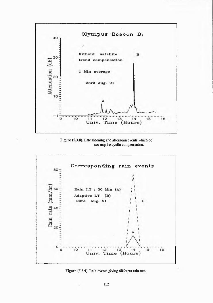
O ly m p u s B e a c o n Bj

Figure (5.3.8). Late morning and afternoon events which do not require cyclic compensation.

C o r r e s p o n d i n g r a i n e ven ts

Figure (5.3.9). Rain events giving different rain rate.

112

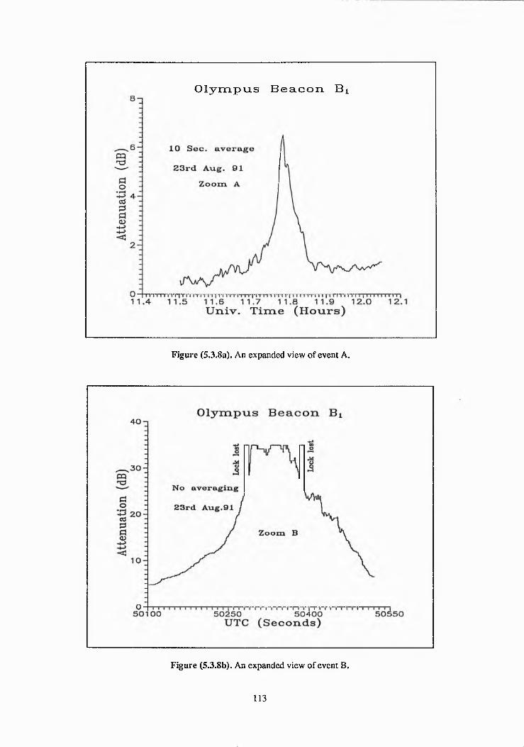
O l y m p u s B e a c o n B ±

Figure (5.3.8a). An expanded view of event A.

Figure (5.3.8b). An expanded view o f event B.

113

O ly m p u s B e a c o n Bi

Univ. Time (H onrs )

Figure (5.3.10). Before cyclic variation compensation.

Figure (5.3.11). Rain events giving accumulated rain.

114

O ly m p u s B e a c o n B A

Figure (5.3.12). After cyclic variation compensation.

Univ. T im e (H on rs )

Figure (5.3.10a). An expanded view o f event A.

115

O ly m p u s B e a c o n Bi

Figure (5.3.13). Before cyclic variation compensation.

C o r r e s p o n d in g r a i n e v e n t s

Figure (5.3.14). Rain events giving accumulated rain.

116

O ly m p u s B e a c o n Bi

U n i v . T i m e ( H o n r s )

Figure (5.3.15). After cyclic variation compensation.

2 0 - i

16-P3"ft

ftoftftft<D

1 2

8 -

Olyixipus B e a c o n

10 S e c . a v e r a g e

"i—i—i— \—r* 1 6.0

t— i— |— i— i— i— i— r

1 6 .5n— r~ i— i ■ r~ i— r i — |—n — i—i— m — r~ i—

17.0 1 7 .5 1 8 .0U n i v . T i m e ( H o n r s )

• Figure (5.3.13a). An expanded view o f eyent A.

117

No. o

f oc

cure

nce

f 1

HISTOGRAM PRESENTATION

90

80

70

60

50

40

30

20

10

0-5 0 5 10 15 20 25 30 35 40

Attenuation (dB)

Figure (5.3.16). A histogram presentation of fade events.

118

Date: 1st Aug. 91

Satellite drift error +2 dB

No. o

f oc

curr

ence

f F

250

200

150

100

50

H I S T O G R A M P R E S E N T A T I O N

“i---------- 1----------1---------- r

Date: 22nd Aug. 91

Satellite drift error +2 dB

_ i________|_____________u0 2 4 6 8 10 12 14

Attenuation (dB)

Figure (5.3.17):. A histogram presentation of fade events.

J119

HISTOGRAM PRESENTATION

Date: 23rd Aug. 91

Satellite drift error +2 dB

■5 0 5 10 15 20 25 30 35 40

Attenuation (dB)

Figure (5.3.18)i A histogram presentation of fade events.

No.

of oc

cure

nce

//

HISTOGRAM PRESENTATION

350

300 -

2 5 0 -

200 -

150-

100 -

50

Date: 22nd and 23rd Aug. 91

Satellite drift error +2 d B

0 10 15 20

Attenuation (dB)

Figure (5.3.19). A histogram presentation of fade events.

25 30 35 40

J121

25

H IST O G R A M P R E SE N T A T IO N

o

o*5

20-

15-

10

Date: 22nd Sep. 91

Satellite drift error +2 dB

1 2 3 4

Attenuation (dB)

Figure (5.3.20). A histogram presentation of fade events.

J122

HISTOGRAM PRESENTATION

900

800

700

600

500

400

300

200

100

0

Date: 28th Sep. 91

Satellite drift error +2 d B

t— r2 4 6 8 10 12 14 16 18

Attenuation (dB)

Figure (5.3.21). A histogram presentation of fade events.

V5: J123

(F

H IST O G R A M P R E S E N T A T IO N

1000

900

800

700<DI 600g

8 500 *oo 400Z

300

200

100

0-2 0 2 4 6 8 10 12 14 16 18

Attenuation (dB)Figure (5.3.22). A histogram presentation of fade events.

Date: 22nd and 28th Sep.91

Satellite drift error +2 dB

J124

MAYAK B e a c o n

Figure (5.4.1.1). Event based fade duration distribution.

O ly m p u s B e a c o n Bi

Figure (5.4.1.2). Event based fade duration distribution.

125

jI

O ly m p u s B e a c o n

Figure (5.4.1.3). Event based fade duration distribution.

O ly m p u s B e a c o n Bi

Figure (5.4 J. 4)&Eveo.Lb&sed-fade duration distribution.

126

O ly m p u s B e a c o n Bj

Figure (5.4.1.5). Event based fade duration distribution.

Figure (5.4X 6)..E vent based fade duration distribution.

127

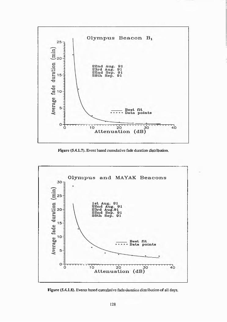
Figure (5.4.1.7). Event based cumulative fade duration distribution.

O ly m p u s a n d MAYAK B e a c o n s

Figure (5.4.1.8). Events based cumulative distribution-of all days.

128

MAYAK Beacon.

10 100P e r c e n t a g e o f e v e n t t i m e a t t e n u a t i o n e x c e e d e d

Figure (5.5.1). Event based attenuation distribution.

O ly m p u s B e a c o n B.

P e r c e n t a g e o f e v e n t t i m e a t t e n u a t i o n e x c e e d e d

Figure (5.5.2). Events based attenuation distribution.

129

O ly m p u s B e a c o n B x

1 10 1 o oP e r c e n t a g e o f e v e n t t i m e a t t e n u a t i o n e x c e e d e d

Figure (5.5.3). Event based attenuation distribution.

O ly m p u s B e a c o n

P e r c e n t a g e o f e v e n t t i m e a t t e n u a t i o n e x c e e d e d

Figure (5.5.4). Events based attenuation distribution o f two days.

130

O ly m p u s B e a c o n Bt

0.001 0.01 0.1 1 10 iooP e r c e n t a g e o f e v e n t t i m e a t t e n u a t i o n e x c e e d e d

Figure (5.5.5). Event based attenuation distribution of two days.

Figure (5.5.6). Events based cumulative attenuation distribution o f two days.

131

<r

CUMULATIVE ATTENUATION DISTRIBUTION

O ly m p u s a n d MAYAK B e a c o n s

Figure (5.5.7). Events based cumulative attenuation distribution of all days.

J

132

P r e d i c t e d a n d M e a s u r e d D a t a

Figure (5.6.1). A comparison between measured beacons data and C C I R rain attenuationmodel prediction for Guildford.

P r e d i c t e d a n d M e a s u r e d D a t a

P e rc e n ta g e of a n average y e a r a t t e n u a t i o n e x ceed ed

Figure (5.6.2). A comparison between measured beacons data and Crane's rain attenuatioQ^^-.^^..prediction for Guildford.

133

P r e d i c t e d a n d M e a s u r e d D a t a

P e rc e n ta g e of an average y e a r a t t e n u a t i o n exceeded

Figure (5.6.3). A comparison between measured beacons data and S A M ’s rain attenuationprediction for Guildford.

P r e d i c t e d a n d M e a s u r e d D a ta

0.01 0.1 1 P e r c e n t a g e o f a n a v e ra g e y e a r a t t e n u a t io n e x c e e d e d

Figure between measured beacons data and Lin's rain attenuationprediction for Guildford.

134

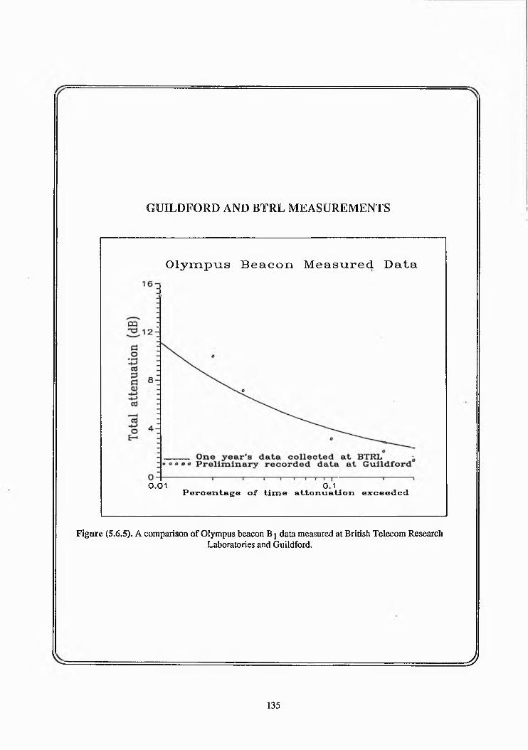
GUILDFORD AND BTRL MEASUREMENTS

O ly m p u s B e a c o n M e a s u r e d D a t a

0.01 0.1P e r c e n t a g e o f t i m e a t t e n u a t i o n e x c e e d e d

Figure (5.6.5). A comparison of Olympus beacon B j data measured at British Telecom ResearchLaboratories and Guildford.

J

135

CHAPTER 6

CONCLUSION AND FUTURE WORK

In this thesis a brief history of satellite communication developments is presented, including the latest work on radio wave propagation studies in ka frequency band. The design and testing of the experimental arrangement for receiving and down converting of the B\ beacon signal together with the weather station arrangement for data logging, display, and analysis is described. Some analysis of segmented recorded data, over a period of four months, is also discussed.

The weather data acquisition software (PCW) was supplied with the weather station. It has been modified (MPCW) and a new time integration method has been introduced, called adaptive integration time, for better results. This method has proved useful for the calculation of rain rate from the recorded data of high rainfall (for longer duration) using low resolution rain gauge, RG2, (see fig. 5.3.9). However, this time integration technique could not be used for scattered showers because of the resolution limitation of the rainguage (see fig. 5.3.14). A good correlation between rain and corresponding fade depth can be seen from the beacon data and the weather station data, as shown in fig.(5.3.3), (5.3.4), (5.3.8), and (5.3.9). On the other hand there is not a good correlation between accumulated rain recorded and rain attenuation in fig. (5.3.10), (5.3.11) and fig. (5.3.13), (5.3.14). There are two reasons for this disagreement:

© The RG2 was a slow rain gauge with 2.54 mm resolution.© Data logging intervals for rain were 30 minutes.

Olympus orbit control system had problems which resulted in the loss of the satellite, this caused interruption in the propagation data collection. In its absence transmission from the Russian satellite, MAYAK, was received at elevation angle of 29.9°; receiving equipment for beacon measurements was modified accordingly. A limited propagation data was collected due to the short time availability of the satellite. However, during this brief period of time rain attenuation of greater than 35 dB was recorded, as shown in fig.(5.3.3). Clear sky peak to peak diurnal variation of about 18 dB was observed, as shown in fig. (5.2.1). This diurnal variation can be divided into two equal sections. The maximum cyclic variation existed in the first twelve hours of the day while in the second

136

half relatively little variation of about 6 dB was present. Large variation of this type could make statistical analysis unproductive. Nevertheless, compensation of the cyclic variation at the data pre-processing stage has yielded more meaningful results.

Olympus was restored on 14th August 1991, the experimental arrangement was again modified and the data collection campaign continued as initially planed. Olympus showed cyclic variation after its recovery like MAYAK but the maximum clear sky peak to peak variation was about 4 dB as shown in fig. (5.2.2). Once again, the software compensation of unwanted daily variation was utilised. Event based analysis of the preliminary recorded data, after compensation for the cyclic variation, was carried out.

Fade events >35 dB were observed from MAYAK as well as Olympus beacons. Rain fade statistics obtained were compared with some rain attenuation prediction models, discussed in chapter 3. The measurements taken have shown good agreement at high percentage of time while agreed less well at low percentages with prediction models, due to the following reasons:

© The recorded data was limited.• Deep fades occurred for high percentage of event time which normally take place

rarely and contribute towards low percentage of the year.

However, Crane rain attenuation prediction is in good agreement with the limited measured data, as shown in fig. (5.6.2). It would be interesting to compare the min attenuation prediction of all models, mentioned above, with long term observed rain and beacon measured data.

The limited data set was compared with the one year’s data collected at BTRL, as shown in fig. (5.6.5). Once again both measurements are comparable for high percentage of time but do not agree at low percentages; the fore mentioned reasons seems the most likely cause for disagreement. More data is needed for better comparison with other UK experimenters. This is quite possible since the experimental arrangement has been established and Olympus will be in the geostationary orbital location of 19° W for approximately one more year. Moreover, the data recording is in progress.

Fade interval or fade frequency statistics was compared with the Swedish/Danish measurements at 1, 2, 3 and 5 dB fade levels. The results showed good agreement. The

137

reason of such correlation is that both measurements were taken over short period of time.

Positive and negative fade rate statistics were obtained which revealed that both had similar distributions. The DBR1-S cannot measure fade rate greater than 5 dB. Therefore, maximum fade rate of >5 dB/sec can be inferred from the measurements. It was also observed that higher attenuation resulted in higher fade rate. Beacon measurements were taken over a period of about four months which were interrupted several times due to the loss of Olympus and hardware and software developments for alternative satellite. During this period of four months only fifteen significant propagation events were recorded and analysed. Some of the fade events were as deep as 35 dB. This time of the year can be declared as quite significant from propagation measurements point of view. However, the measurements taken so far can be concluded as:

Table (6.1). Statistics obtained over a period of four months.% of event time 0.1 1 10Attenuation (dB) >35 13.5 3

Table (6.2). Fade duration statistics.Mean fade duration

3 dB 5 dB 10 dB 20 dB 30 dB 35 dB> 20 min 9 min 3 min 1 min 30 sec < 30 sec 1

Table (6.3). Positive and negative fade rates.Fade rate Positive Negative

Maximum >5 dB/sec >5 dB/sec

................ TyP'ca* 1.3 dB/sec 1.2 dB 1

Until now only copolar attenuation measurements have taken and analysed. Although cross polar measurements of Bj were taken these have not been analysed due to some problems with the beacon receiver which resulted in spikes in the cross polar measurements. Furthermore, no scintillations were observed so far. Scintillations can be a problem at ka bands. More propagation data and analysis is required in order to quantify the scintillations effect at 20 GHz.

138

In May 1992 a new beacon data acquisition software was introduced [Otung, 1993] which allows data recording in DAPPER's format. Measurement of relative humidity is required for DAPPER pre-processing and analysis package.

No measurements of relative humidity have been made. Its effects on radio waves at 20 GHz can be of some interest as this frequency is near the water absorption peak at 22.3 GHz.

It is mentioned earlier that rain gauge RG2 is useful for high rainfall with MPCW weather data acquisition software but light rainfall, as shown in fig. (5.3.14), cannot be recorded meaningfully. Deficiency of this type can be compensated by operating a fast rain gauge in conjunction with RG2. Horizontal rain extent can be obtained with a network of rain gauges along the slant path. The data from the network can be used for a feasibility of installing another antenna tens of meters from the first antenna as a form for site diversity; this may prove to be an economical and effective form of fade counter measure. Moreover, long term rain and beacon measurements can be continued, and the data will be very useful for empirical rain attenuation models development.

139

REFERENCES

Allnutt. J. E [1989]"Satellite to Ground Radiowave Propagation".IEE Electromagnetic waves series 29. Published by Peter Peregrinus Ltd.

Altshuler. E.E [1984]"A simple expression for estimating attenuation by fog at millimetre wavelength".IEEE Trans, on Antenna and propagation. Vol. AP-32, No. 7 P 757-758.

Arnold. H. W , Cox. D. C and Hoffman. H. H [1977]"Attenuation and depolarisation measurements at Crawford Hill using the C O M S T A R beacons".Paper presented at commission F, UNSC/URSI meeting, Union Radio Sci. Inst Stanford University of Stanford, California, June 23,1977.

Arnold. H .W and Cox. D. C [1978]."Dependence of depolarisation on incident polarisation for 19 G H z satellite signals".Bell system Technical Journal Vol. 57, P 3267-3276.

ATS-6 [1977]Proceedings of ATS-6 meeting E S T E C (ESA SP-131, Oct. 1977), 6th-7th Sep. 1977.

Belshaw. J. C [1991].Private Communication.

Belshaw. J. C [1992].Private Communication.

Bodtmann. W. F and Ruthroff. C. L [1974]"Rain attenuation on short radio paths: Theory, experiment and design".Bell System Technical Journal Sep. 1974 P 1329-1349.

Bostain. C. W et al [1975]"Depolarisation measurements on the A T S -6 20 G H z down link".IEEE Trans. M T T - 23, P 1049-1053.

Bostain. C. W and Allnutt. J. E [1979]"Ice-Crystal depolarisation on satellite-earth microwave radio paths".Proc. IEE Vol. 126, No. 10, P 951-960.

CCIR Report 564- 3 [1986]"Propagation in non ionised media".Recommendations and Reports of the CCIR, 1986, ITU, Geneva Volume 5, P 389-431.

CCIR Report 563-4 [1990]"Propagation in non ionised media".Recommendations and Reports of the CCIR, 1986, ITU, Geneva Volume 5, P 105-148.

CCIR Report 564-4 [1990]"Propagation in non ionised media".Recommendations and Reports of the CCIR, ITU, Geneva Volume 5, P 447-505.

140

CCIR Report 719-3 [1990]"Propagation in non ionised media".Recommendations and Reports of the CCIR, ITU, Geneva Volume 5, P 189-204.

CCIR Report 720-2 [1990]"Propagation in non ionised media".Recommendations and Reports of the CCIR, ITU, Geneva Volume 5, P 205-225.

CCIR Report 721-3 [1990]"Propagation in non ionised media".Recommendations and Reports of the CCIR, ITU, Geneva Volume 5, P 226-245.

Chetty, P. R. K [1991]"Satellite Technology and its application".2nd edition T A B Professional and Reference Book.

Clark, A. C [1945]"Extra terrestrial relays".Wireless world October, P305-308.

Cox. D. C, Arnold. H. W. and Hoffman [1978]"Depolarisation of 19 and 28 G H z earth-space signals by ice particles".Radio Science Vol. 13, P 511-517.

Crane. R. K [1971]"Propagation phenomena affecting millimetre wavelength bands".Proc. IEEE Vol. 59, No. 2, P 173-188.

Crane. R. K [1978]"A Global model for rain attenuation prediction".E A S C O N Record P 391-395.

Crane. R. K and Blood. D [1979]"Hand book for the estimation of microwave propagation effects-Link calculations for earth space paths". Environment Research and Technology Report No. 1, P 7373-TRL.

Crane. R. K [1980]"Prediction of attenuation by rain".IEEE Trans. C O M -28 (9), P 1717-1733.

Crane. R. K [1982]"A two component rain model for the prediction of attenuation statistics".Radio Science Vol. 17, No. 6, P 1371-1387.

Crane. R. K [1985]"Evaluation of Global and CCIR models for estimation of rain rate statistics".Radio Science Vol. 20, No. 4, P 865-879.

Davies. P. G and Mackenzie. E. C [1981]Review of S H F and E H F slant path propagation measurements made near Slough".Proc. IEE Vol. 128, Part H, No. 1, P 53-65.

DBRl-S Manual [1991]"DBR1 -S Digital Beacon Receiver Manual".

141

Dintelmann. F [1981]Analysis of 11 G H z slant path fade duration and fade slope".Electronic Letters Vol. 17, No. 7, P 267-268.

E S A Doc. [1990]"Olympus in orbit testing final report".CCE/54507/CM/AP Issue No. 1.European Space Research and Technology Centre (ESTEC), Noordwijk, Netherlands.

Evans. B . G [1991]"Satellite Communication systems".EEE Telecommunication Series No. lS.Published by Peter Peregrinus Limited.

Evans. B. G and Holt. A. R [1977]"Scattering amplitude and cross polarisation of ice particles".Electronic Letters Vol. 13, P 342-344.

Fugono, N and Hayashi, R [1978]"Propagation Experiment in 1.7,11.5 and 34.5 G H z with Engineering Test Satellite Type II".Paper 78-623, A I A A 7th Communication Satellite Systems Conference (April).

Fugono, N. Hayashi, R et al. [1980]"ETS-II Experiments Part I: Japan's First Geostationary Satellite".IEEE Trans, on Aerospace and Electronic Systems, Vol. AES-16 no. 5, P549-557.

Fukuchi, H. Kozu, T et al [1983]"Centimetre W a v e Propagation Experiments Using the Beacon Signals of CS and B S E Satellites”.IEEE Trans, on antennas and propagation, Vol. AP-31, P603-613.

Giannone, B et al. [1986]"Exploitation of the 20-40-50 G H z Bands: Propagation Experiments with Italsat".Paper 86-0650, A I A A 11th Communication Satellite Systems Conference (March).

Gibbins. C. J [1986]"Improved algorithms for the determination of specific attenuation at sea level by dry air and water vapour, in the frequency range 1-350 GHz".Radio Science Vol. 21, No. 6, P 945-954.

Harris, J. M and Hyde, Y [1977]"Preliminary results of C O M S T A R 19/29 G H z beacon measurements at Clarksburg, Maryland". C O M S T A R Technical Review Vol 7, No. 2 P599-623.

Hogg. D. C and Chu. T. S [1975]"The role of rain in satellite communications".IEEE Trans, on Antenna and Propagation Vol. 63, No. 9, P 1309-1351.

Howell, R. G, Harris, J. W et al. [1991]" O L Y M P U S 12, 20 and 30 G H z slant path attenuation and radiometric measurements at B T R L Martlesham".Proc. EEE Conf. ICAP91, IEE Conf. Pub. No. 333.

Issue No. 1, Jan. 1991. Signal Processors Limited, Cambridge, UK.

142

Hyde, K. G [1975]"ATS-6 preliminary results from the 13/18 G H z C O M S T A R propagation experiment".Special issue on ATS-6 IEEE Trans, on Aerospace and Electronic System Vol. 11, No.6.

Ippolito, L. J [1976]"Characterisation of the CT S 12 and 14 G H z communication iinks-Preliminary Measurements and Evaluation".International Conference on Communications: ICC 76 (June).

Ippolito. L. J. [1986]"Radiowave Propagation in Satellite Communication".Published by Van Nostrard Reirhold, USA.

Ippolito. L. J [1989]"Propagation Effects Handbook for Satellite System Design".Published by NASA, Publication No. 1082(04), Feb. 1989.

Jeay, Y [1991]"Propagation experimentM. Sc. (Thesis). University of Surrey, UK.

Karasawa. Y, Yasukawa. IC and \ amada. M [1988]Tropospheric scintillation in the 14/11 G H z bands on earth-space paths with low elevation angles".IEEE Trans, on Antenna and Propagation AP-36, P 563-569.

Larsen. J. R [1991]"Duration and interval data on attenuation and X P D ”.Paper presented on first O P E X workshop held between 23rd -24th April 1991 at ESTEC, Netherlands. P 4.1.1-4.1.7.

Leitao. M. J and Watson. P. A [1986]"Method for prediction of attenuation on earth-space links based on radar measurements of the physical structure".Proc. IEE Vol. 133, Part F, No. 4, P 429-440.

Lin, S. H [1978]"Empirical calculations of microwave rain attenuations on earth-space satellite paths".Record E A S C O N ’ 78 held Arlington, V A P 372-378.

Lin. S. H, Bergmann. H. J and Pursley. M. V [1980]"Rain attenuation on earth-satellite paths-Summary of 10 years experiments and studies".Bell System Technical Journal Vol. 59, No. 2, P 183-228.

Martin, D. H [1991]"Communication satellites 1958-1992".The Aerospace corporation, El Segundo, California 90245.

Martinino. F et al. [1992]"The I T A L S A T system: current applications and future trends".Space Communications Vol. 10, P67-82.

Matricciani. E [1981]Rate of change of signal attenuation from SIRIO at 11.6 GHz".Electronic Letters Vol. 17, No. 3, P 139-141.

143

McCormick. G. C and Hendry. A [1977]"Depolarisation by solid hydrometeors".Electronic Letters Vol. 13, P 83-84.

Meredith. A. H [1987]"Considerations in the development of a communications network employing satellites operating in the 20/30 G H z frequency band".M. Sc. (Thesis) University of Surrey.

Merlo. U. E and Macchetti. P. G [1985]Amplitude scintillation cycles in a SIRIO satellite earth link".Electronic Letters Vol. 21, No. 23, P 1049-1096.

Miya. K [1985]"Satellite Communication Technology"."Published by K D D Engineering and Consulting Inc. Tokyo.

Morgan. W . L and Gordon. G. D [1988]"Communication Satellite Handbook".Published by John Wiley and Sons, USA.

Moupfouma. F [1987]"More about rainfall rates and their predictions for radio system engineering".Proc. IEE Vol. 134, Part H, No. 6, P 527-537.

Oguchi. T [1983]"Electromagnetic wave propagation and scattering in rain and other hydrometeors".Proc. IEEE Vol. 71, No. 9, P 1029-1078.

Olsen. R. L [1978]" The aRB in the calculation of rain attenuation".IEEE Trans, on Antennas and Propagation Vol. AP-26, P 318-329.

Otung, I [1993]Private communication.

Pratt, T and Bostain, C. W [1986]"Satellite Communication".John Wiley and Sons Inc.

Pruppacher. H. R and Pitter. R. L [1971]"A semi-empirical determination of the shape of the cloud and rain drops".Journal of the Atmospheric Science Vol. 28, P 86-94.

Ramat, P [1979]"Propagation measurements on a satellite earth path through SIRIO Experimental satellite".Alta frequenza Vol. 48, no. 6 (June)

Ransome. P. D [1989]"Prototype digital beacon receiver for the Olympus satellite".Final Report of ESA, E S T E C contract no. 6910/86/NL/JG(SC).

144

Ransome. P. D [1990]Private Communication.

Ransome. P. D [1992]Private Communication.

Rees, D. W,E[1990]"Satellite Communication".

Rucker. F [1991]"Description of the dynamic behaviour of the Olympus beacon signals by the signal variance and fade slope".Not published. Author is working in Forschungsinstitut. der Deutschen Bundespost Telekom D-6100 Darmstadt. Federal Republic of Germany.

Saunders. M. J [1971]"Cross polarisation at 18 and 30 G H z due to rain".EEEE Trans, on Antennas and Propagation Vol. 19, Part 2, P 273-277.

Schmeller, O [1986]"The German Telecommunication Satellite System DFS-Kopemikus".Paper 86-0695, A I A A 11th Communication Satellite System Conference (March).

Slobin. S. D [1982]"Microwave noise temperature and attenuation of clouds".Radio Science Vol. 17, No. 6, P 1443-1454.

Stutzman. W. L and Dishman. W. IC [1982]"A simple model for the estimation of rain induced attenuation along earth space paths at millimetre wavelengths".Radio Science Vol. 17, No. 6, P 1465-1476.

Stutzman. W. L and Dishman. W. IC [1984]Correction to "A simple model for the estimation of ram induced attenuation along earth space paths at millimetre wavelengths".Radio Science Vol. 19, No. 3, P 946.

Stutzman. W. L and Yon. K. M [1986]"A simple rain attenuation model for earth space radio link operating at 10-35 GHz".Radio Science Vol. 21, No. 1, P 65-72.

Thirlwell. J and Howell. R. G [1980]"20 and 30 G H z slant-path propagation measurements at Martlesham Heath, UK".A G A R D Conference Proc. No. 284, P 10.1-10.9.

Tremurici, D [1990]"Payload Design and Repeater Performance of DF S Kopemikus 1".Space Communications Vol. 7, no. 4-6 (November).

Tsukamoto, IC [1978]"Technical Aspects of the Japanese Broadcasting Satellite Experiments".IEEE Trans, on Broadcasting, Vol. 24, no. 4 (December).

145

Tuar. R. R [1973]"Ionospheric Scintillation at 4 and 6 GHz". C O M S T A R Technical Review Vol. 3, P 145-163.

Watson. P. A [1978]"A summary and assessment of the 20/30 G H z ATS-6 propagation data collected during the European phase".Proc. of symposium on Advanced Satellite Communications System, Genoa, Italy, 14th -16th Dec. 1977. (ESA SP-138 Jan. 1978) P 245-249.

Weiner. K [1982]"The UHF-Compendium".Part 1 and Part 2.Published by Radio Society Great Britain.

Wilkins. D. E. B [1992]Private Communication

Yamada. M, Karasawa. Y and Yasunaga. M et al [1987]"An improved prediction method for rain attenuation in satellite communication operating at 10-20 GHz".Radio Science Vol. 22, P 1053-1062.

146

APPENDIX I

B A N D P A S S F I L T E R

This filter has narrow-band properties and was intended to be used as bandpass (1223 MHz) or to fdter out other undesired frequencies. Optimized coupling and the specific arrangement of the lines ensure minimum losses in conjection with narrow bandwidth. The filter construction is governed by the internal dimensions which were 60x60x20 mm. LI, L2 and L3 (6 m m dia.) and die case consists of solid brass. LI and L3 measures 54.4 m m each and L2 is 50 m m long, as shown in fig. (A-I 1). Again all components are assembled by means of bolts inserted from the outside. Capacitive tuning is provided through SI, S2 and S3 bolts and lock-nuts. Soldering tags were inserted at the cold ends of LI and L3. Both cover plates (measuring 70x75 m m ) were screwed to the frame which is composed of four parts using twelve screws per coverJFrequency response of the filter is shown in fig. (A-I 2).

The filter design was altered in order to be used as bandpass (1045 MHz) or to filter out the bulk of the other frequencies arriving as a result of the first downconversion. Internal dimensions of the filter were modified as 72x72x20 mm, which was quarter wavelength of centre frequency, i.e 1045 MHz.

147

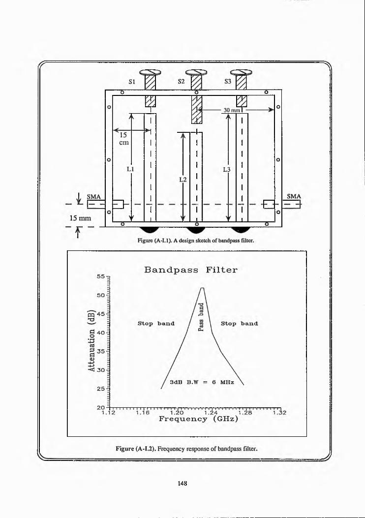
148

APPENDIX II

PCW INTERFACING CARD

A description about the port selection and modification, which was carried out, is presented in this section. A sketch of Personal Computer Weather (PCW) interfacing card is shown in fig. (A-II. 1) and fig. (A-ll. 2) gives an expanded view of port selection area marked with 1 to 7 as trace reference. The default base address for P C W was 300 (hex). Since another peripheral was already present with the same base address, therefore trace 3 was selected and trace 5 was disconnected. A list of base address for other selection lines is given in Table (A-II. 1). Any port can be selected by connecting one of the seven vertical traces to the horizontal trace and M P C W (Modified Personal Computer Weather; modified weather data acquisition, see appendix III) programme can be executed followed by forward slash and port address, e.g. MPCW/280. Table (A-II. 1). List of ports address.

Table (A-II. 1). List of ports address.

Trace Ports address I B M use1 200 Game port2 240 Unused3 280 Proto card4 2C0 Unused5 300 Unused6 340 Unused7 380 Unused

149

1 5 0

APPENDIX IIIM P C W D A T A A C Q U I S I T I O N

/* The name of the programme is: N P C W (New Personal Computer Weather *//* The existing weather acquisition software called P C W (Personal Computer Weather ) was modified */

#include <dos.h> /* Contains R E G S definition for calls to M S - D O S or *//* video interrupts; also contains MK_FP() which is */I* used to create the pointers to the P C W data block. */

#include <stdio.h> /* Basic screen I/O */

#define D A T A _ O F F S E T 516 #define U P D A T E _ O F F S E T 514 #defme V I D E O 0x10

/* Offset of data in P C W program */ /* Offset of update control byte */

/* BIOS video interrupt number */

union R E G S regs; /* register pack for interrupt calls */

*//* P C W keeps its passable data in a collective memory block./* In Turbo-C we can define this block as a single structure *//* with d u m m y variables covering what is not normally accessed. */ /* W e can then access the data using the pointer->field method. */ I* Should we want to access only a few registers, each may have- */ /* its own pointer. Note that all pointers into the P C W block *//* must be declared as being of far or huge type. See below. */

typedef struct /* For separate pointers, each would add its offset */ /* listed below to the basic pcwsegment():DATA_OFFSET

{ /* pointer: */*/

*/int hour; /* +0 : Time of day; hour (24 hour format) int minute; /* +2 : Time of day: minutes */int second; /* +4 : Time of day: seconds*/int day; /* +6 : Day of the month*/ int month; /* +8 : Month of the year */ int year; /* +10 : Year */ int dO; /* (not accessed) */int relbar; /* +14 : Relative barometric pressure (in inches x 100) */ int dl; /* (not accessed) */int d2; /* (not accessed) */int templ;/*+20: Temperature l(in xF X 10) */ int templlo; /* +22: Lowest reading of temperature 1 (in 10) int tempi hi; /* +24 : Highest reading of temperature 1 (in 10) int temp2; /* +26 : Temperature 2 (in 10)*/ int temp21o; /* +28 ; Lowest reading of temperature 2 (in int temp2hi; /* +30 ; Highest reading of temperature 2 (in 10) int windsp; /* +32 : Wind speed (in M P H ) */int windav; /* +34 ; Average of 60 wind speed samples */int windhi; /* +36 : Highest recorded wind speed (in M P H ) */ int windch; /* +38 : Wind chill factor (in 10) */int windchlo; /* +40 : Lowest recorded wind chill factor (in 10) */ int d3; /* (not accessed) */int winddir; /* +44 : Wind direction (in degrees) */

10) */10) */

10) */10) */

151

int raindly; /* +46 : Accumulated daily rainfall (in inches x 10) */int rainann; /* +48 : Accumulated annual rainfall (in inches x 10) */

} pcwdata;

pcwdata far *dblk; /* dblk is pointer to PCW's datablock. *//* It is defined in initptrs(). */

/* Note the definition of the datablock pointer above as a far pointer *//* to a structure. As an example of separate pointers, die three time of *//* day registers could be accessed with far pointers to integers, which *//* might be defined as follows: */j*/* int far * t im e _ h o u r , *tirne_minute, *time_second; */

j/* or whatever labels you prefer. */

char far *update; /* Actual machine address of timing register. */ /* The background routine will continue *//* to refresh data once per second while *//* this register is non-zero. Each second *//* the routine decrements this register *//* until it reaches zero. Once the register *//* reaches zero, updates are once per minute. *//* To request updates every second for the *//* next 30 seconds, just put the value 30 in */!* this register. */

/* Function declarations */

int pcwsegment(void); int pcwthere(void); void initptrs(void); void cursoroff(void); void cursoron(void); void clrscr( void);

/* find segment for pointers */ /* see if pew is installed *//* initialize pointers *//* turn cursor off *//* turn cursor on */

/* clear the screenvoid cursorto(int row, int column); /* position cursor on screen */

/* The following program simply reads the time of day, barometer, and */ /* temperature 1, and displays them on the screen. The cursor control *//* and clear-screen functions are not defined in Turbo-C and must be */ /* supplied by the user, either explicitly or from within a library. */ int newtime, oldtime=00; float newtempl, oldtemp 1=0.0; float newtemp2, oldtemp2=0.0; float newArain, oldArain=0.0; float Hour, Min, Sec, time; float Rltime=0.00; float RBtime=0.00; float Rrate, tflag; mainO (

clrscrO; if (pewthereQ)

152

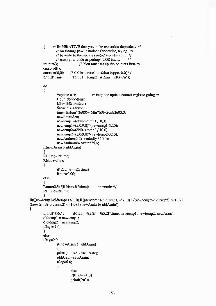
{ /* I M P E R A T I V E that you make execution dependent *//* on finding pew installed! Otherwise, trying *//* to write to the update control register could *//* trash your code or perhaps D O S itself. */

initptrsQ; /* You must set up the pointers first. */cursoroffO;cursorto(0,0); /* 0,0 is "home" position (upper left) */ printf("Time Tempi Temp2 ARain RRateXn");

do{

^update = 4; /* keep the update control register going */Hour=dblk->hour;Min=dblk->minute;Sec=dblk->second;time=((Hour*3600)+(Min*60)+Sec)/3600.0;newtime=Sec;newtemp l=(dblk->temp I / 10.0); newtemp 1=(5.0/9.0)* (ne wtemp 1 -32.0); newtemp2=(dblk->temp2 / 10.0); newtemp2=(5.0/9.0)*(newtemp2-32.0); newArain=(dblk->raindly / 10.0); newArain=newArain*25.4;

if(newArain > oldArain){RBtime=RItime;RItime=time;}

if(RItime=RBtime)Rrate=0.00;

else{Rrate=2.54/(RItime-R Btime); /* mra/hr */RBtime=RItime;}

if(((newtempl-oldtempl) > 1.0) II ((newtemp 1-oldtempl) < -1.0) II ((newtemp2-oldtemp2) > 1.0) II ((newtemp2-oldtemp2) < -1.0) II (newArain != oldArain)){

printf("%6.4f %5.2f %5.2f %5.2f,time, newtemp 1, newtemp2, newArain);oldtempl = newtemp 1; oldtemp2 = newtemp2; tflag = 1.0;}elsetflag=0.0;

if(newArain != oldArain){printf(" %5.2f\n",Rrate);oIdArain=newArain;tflag=0.0;}

elseif(tflag==1.0)printf('tNn");

153

}whilc(!(kbhitO));

) /* all this if pew is installed in background */elseputs("PROGRAM A B O R T E D : P C W program did not respond to function calls.");

cursoronQ;

/*PCW P R O G R A M F U N C T I O N S */

/* D O S C A L L 70(HEX) IS U S E D B Y P C W F O R PA S S I N G P C W */ f* I N F O R M A T I O N . THIS IS (SO FAR) U N U S E D B Y DOS. (IF A L L *//* T H E C P U R E GISTERS A R E N O T A S DEFINED, T H E N T H E F U N C T I O N /* C A L L IS P A S S E D T O DOS.) */

___________________________ *i/* B X = $6060 ( R E T U R N S E G M E N T IN AX) *//* B X = $7070 ( C H A N G E A L L $7070 REG. T O $0070) *//* ( U S E D T O VERI F Y T H A T P C W IS INSTALLED) *//* B X = $8080 ( U N I NSTALL P C W A N D F R E E M E M O R Y ) *//* *//* A X = $7070 *//* C X = $7070 *//* D X = $7070 *//* SI = $7070 *//* DI = $7070 *//* BP,SP,CS,DS & ES A R E N O T D E F I N E D */

j* pcwsegmentO uses the "return segment" function of pew program. */ f* B X = $6060 requests this function. The other registers are set *//* to $7070 so that the pew program recognizes the function request. */

int pcwsegment(void){regs.x.ax = 0x7070; /* set all registers prior to dos call */regs.x.bx = 0x6060;regs.x.cx = 0x7070;regs.x.dx = 0x7070;regs.x.si = 0x7070;regs.x.di = 0x7070;

/* interrupt call returns segment *//* of P C W datablock in ax register, *//* which is passed as return value *//* of intdosO function, and is in *//* turn passed as return value of *//* pcwsegmentO* */

retum(intdos(&regs, &regs));}

/* pcwthereQ uses the "acknowledge presence" function of pew program. */ /* B X = $7070 requests this function. The other registers are set to */

154

/* $7070 so that the pew program recognizes the function request. */ int pcwthere(void){regs.x.ax = 0x7070; /* set all registers prior to dos call */regs.x.bx = 0x7070;regs.x.cx = 0x7070;regs.x.dx = 0x7070;regs.x.si = 0x7070;regs.x.di = 0x7070;intdos(&regs, &regs);

/* Returns 0 if any of the six *//* registers is not 0x70, and *//* nonzero if all six are 0x70 */

retum((regs.x.bx == regs.x.cx) & &(regs.x.cx == regs.x.dx) & &

(regs.x.dx == regs.x.si) & &(regs.x.si == regs.x.di) & &

(regs.x.di == 0x70));)

/* initptrsO uses pcwsegment() to find the segment to be used for the */ /* pointers to the pew data block and the update control register. It */ /* then combines this segment with the individual offsets to initialize */ /* the two pointers. */

void initptrs(void){unsigned int i;

update - MKJFP((i = pcwsegmentO), UPDATE_OFFSET); dblk = MK_FP(i, D A T A _ O F F S ET);

}

/* Turn off cursor using BIOS set cursor type routine */

void cursoroff(void){regs.h.ah = 1; /* Select SET C U R S O R T Y P E call */regs.x.cx = 0x2000; /* ch bit 5: cursor off. */int86(VIDEO, &regs, &regs); /* process video call */

}

/* Turn on cursor using BIOS set cursor type routine */

void cursoron(void){regs.h.ah = 1; /* Select SET C U R S O R T Y P E call */regs.x.cx = 0x0607; /* ch lo byte: cursor starts on */

/* character scan line 6 *//* cl lo byte: cursor ends with *//* character scan line 7 */

int86(VIDEO,&regs, &regs); /* process video call */}

155

void clrscr(void){regs.h.ah = 6; /* Select S C R O L L U P call */regs.h.al = 0; /* empty all lines in window */regs.h.bh = 7; /* line fill attribute: */

/* light grey on black. *//* Define scroll window: */

regs.h.ch = 0; /* topmost row: 0 */regs.h.cl = 0; /* leftmost column: 0 */regs.h.dh = 24; /* bottom row; 24 */regs.h.dl = 79; /* rightmost column: 79 */

/* (specifies full screen) */ int86(VIDEO, &regs, &regs); /* process video call */ cursorto(0,0); /* go to top left corner */

}

/* Position the cursor using the BIOS set cursor routine. */

void cursorto(int row, int column){regs.h.ah = 2; /* Select S E T C U R S O R call */regs.h.dh = row; regs.h.dl = column;regs.h.bh = 0; /* Set page number */int86(VIDEO, &regs, &regs); /* process video call */

}

/* Clear the screen using BIOS scroll up routine */

156

APPENDIX IV

DATA PR E -PR O C E SSIN G A ND ANALYSIS PR O G R A M M ES

/* This programme reads two columns and alternative rows. The name of the programme is: Iqra */ #include <stdio.h> /* Calls to M S - D O S */#include <dos.h> /* Basic screen I/O */main Q {

char Infile[20], Outfile[20];float p,q; /* variable names */int n=0,nl-0,rc=0;FILE *a,*b;puts("Input filename:");gets(Infile);a=fopen(Infile,"r");puts("Output filename:");gets(Outfile);b=fopen(OutfiIe,''w“);while(fscanf(a," %I\i\%f\n" ,&p,&q) !=EOF) (/* Scaning I/p file */

{

n+— 1;

if(n-nl>=l) /* Reading alternate rows */{

rc+=l;

if(rc~l)

{

fprintf(b," %f\t\%f\n" ,p,q);

)

else

{

rc=0;

}

nl=n;

}else

{

157

}}}

/* This programme compensates the diurnal variation of OlympusThe name of the programme is : ALFURQAN */

#include <stdio.h>#include <maih.h>

mainO{

float x,w,y;char infile[ 10],outfile[ 10];FILE *f ,*g;

puts("Enter input file name:"); gets(infile);puts("Enter output file name:");gets(outfile);f=fopen(infile, "r");g=fopen(outfile, "w");while (fscanf(f," %l\t%l\s i" (&x,&y) !=EOF)

{ /* Scaning file and removing average daily variation */

w=0.0;w=L00?.e“6*po\v(xs6)"5.56458e~5*pQw(x}5)+Q.Q0Q933665*powk1.4}; w+=”0.00501878*pow(x,3)+0.0320749*pow(x,2)-0.292881!!tx-0.111812; y=y-w;fprintf(g,"%fi%e\n",x>y);}

fclose(0;

fclose(g);}

158

/* This programme divides the data File with required interval. The name of the programme: (dats) data section */

#include <stdio.h>#include <math.h>#include<ctype.h>

mainO{

float x,w,y;char infile[12],outfile[12];FILE *a,*b,*c,*d,*e,*f,*g,*h;puts("Enter input File name:");gets(infile);

a=fopen(infile, "r");b=fopen("h05", "w"); /*0 to 5 dB interval assignment for data file h05 */c=fopen("h610", "w"); /*6 to 10 dB interval assignment for data file h610 */d=fopen("hl 115","w"); /* 11 to 15 dB interval assignment for data file hi 115 */e=fopen("hl620", "w”); /*16 to 20 dB interval assignment for data file hl620 */f=fopen("h2125", "w"); /*21 to 25 dB interval assignment for data file h2125 */g=fopen("h2630", "w"); /*26 to 30 dB interval assignment for data file h2630 */h=fopen("h3135", "w"); /*31 to 35 dB interval assignment for data file h3135 */while (fscanf(a,"%f\n",&x) 1-EOF)

{

if (x>=0 && x<=5) fprintf(b,,,%f\n",x); if (x>=6 && x<-10) fprintf(c,"%f\n",x); if (x>=ll && x<=15) fprintf(d,"%f\n"5x); if (x>=16 && x<-20) fprintf(e," %f\n" ,x); if (x>=21 && x<=25) fprintf(f,"%f\n",x); if (x>=26 && x<=30) fprintf(g,"%f\n",x); if (x>=31 && x<=35)

fprintf(h," %f\n" ,x);)

fclose(f);fclose(g);

159

/* This programme divides the data fde with required duration interval. The name of the programme: fadallr,col. 1 = t31, col. 2 = t32, col. 3 = t33 =t32 -t31, col. 4 = total duration*/

#include <stdio.h> #include <math.h> #include<ctype.h>

mainO{

float x,y;float 131=0.0,151=0.0,tlOl = 0.0,tl51=0.0; float t201=0.0,t251=0.0,t301=0.0,1351=0.0; float t3 2=0.0,t5 2=0.0,tl02=0.0,tl 52=0.0; float t202=0.0,t252=0.0,t302=0.0,t352=0.0; float t33,t53,tl03,tl53,t203,t253,t303,t353; int flag3 = 0, flagS = 0; int flag 10 = 0, flaglS = 0.0, flag20 = 0; int flag25=0, flag30=0, flag35 = 0; float dur3=0.0,dur5 = 0.0,durl0 = 0.0; float durl5=0.0, dur20=0.0, dur25=0.0; float dur30 = 0.0, dur35 = 0.0; char inflle[12],outfile[12];FILE *a,*b,*c,*d,*e,*f,*g,*h,*i,*j; clrscr();printf("\n\t\IN THE NAME OF ALLAH THE BENEFICENT THE MOST MERCIFULNnW);printf("\t\PROCLAIM IN THE NAME OF THY LORD WHO CREATED .\n\n\n\n\n\n");

puts("Enter input file name:"); gets(infile); a=fopen(infile, "r");b=fopen("d03", "w"); f* Opening a file for 3 dB duration */puts("Enter output file name for fade rate:");gets(outfile);

printf("\n\n\n\t SUB_HAAN ALLAH\t\tSUB„HAAN ALLAH\t\tSUB_HAAN ALLAHNn"); c=fopen(outfile,"w");d=fopen("d05","w"); /* Opening a file for 5 dB duration */e=fopen("dlO","w"); /* Opening a file for 10 dB duration */f=fopen("dl5","w"); /* Opening a file for 15 dB duration */g=fopen("d20","w"); /* Opening a file for 20 dB duration */h=fopen("d25","w"); /* Opening a file for 25 dB duration */i=fopen("d30","w"); /* Opening a file for 30 dB duration */j=fopen("d35","w"); /* Opening a file for 35 dB duration */

while (fscanf(a,"%f\t\%f\n",&x,&y) !=EOF){

if (y>=1.5){fprintf(c,"%f\t\%l\n",x,y);]if(y>=3.0)[

if(flag3!=l) (/* Setting a flag for 3 dB fade level */(flag3=l;

160

t31=x;fprintf(b,"%f\T,t31);}

}

else if (flag3==l){t32=x;t33 = t32 - 131;dur3 = dur3 + t33; (/* Total fade duration */fprintf(b,"%f\t",t32);fprintf(b,"%f\t",t33);fprintf(b," %f\n" ,dur3);fprintf(c,“%f\t\%f\n",x,y);flag3 = 0;}

if (y>=5.0) (J* Fade depth */{ 'if(flag5!=l) (J* Setting a flag for 3 dB fade level */

{flag5=l;t51=x;fprintf(d,"%f\t",t51);}

else if (flag5==l) {t52=x;t53 = t52 - t5T;

/* All t..„2 and L..3 are time corresponding to fade depth */ /* for example t51 is tlie time tl when fade is > 5 dB *//* t52 is time t2 when fade level is ^ 5 dB and t53 *//* is t3 when fade level is > 5 dB and so on */

/* Total fade duration of 5 dB */dur5 = dur5 + t53; fprintf(dv"%fvt"st52); fprintf(d,"% fst" ,t53); fprintf(d,"%f\n",dur5); flag5 = 0;}

if (y>=10.0){if(flaglO!=l)

{flag 10=1; tl01=x;fprintf(e,"%l\t",tl01);)

}

(/* Setting a flag for 10 dB fade level */

else if (flagl0==l){

tl02=x;t!03 = tl02 - tlOl;

161

durlO = durlO + 1103; fprintf(e,"%f\t",tl02); fprintf(e,"%l\t",tl03); fprintf(e,"%f\n",durlO); flaglO = 0;

if (y>= 15.0){

/* Total fade duration of 10 dB */

if(flagl5!=l){flagl5=l;tl51=x;fprintf(f,"%f\t",tl51);}

/* Setting a flag for 15 dB fade level */

else if (flag 15— 1){tl52=x;tl53 = tl52 - tl51; durl5 = durl5 + tl53; fprintf(f,"%f\t",tl52); fprintf(f," %f\t" ,t 153); fprintf(f,"%f\n",durl5); flag 15 = 0;}

if (y>=20.0){

/* Total fade duration of 15 dB */

}

if(flag20!=l){flag20=l;t201=x;fprintf(g,,,%f\T,t201);}

(J* Setting a flag for 20 dB fade level */

else if (flag20==l){

t202=x;t203 = t202 - 1201; dur20 = dur20 t203; fprintf(g,"%fvt"st202); fprintf(g,"%f\t",t203); fprintf(g,,,%fin",dur20); flag20 = 0;

(/* Total fade duration of 20 dB */

}if (y>=25.0){

if(flag25!=l){flag25=l;t251=x;fprintf(h,"%f\t",t251); }

(/* Setting a flag for 25 dB fade level */

162

else if (flag25==l){

t252=x;t253 = 1252 -1251;dur25 = dur25 + t253; (/* Total fade duration of 25 dB */fprintf(h,"%f\t",t252);fprintf(h,"%f\t",t253);fprintf(h,"%f\n",dur25);flag25 = 0;

)if (y>=30.0){

if(flag30!=l) (/* Setting a flag for 30 dB fade level */{flag30=l;t301=x;fprintf(i,"%f\t",t301);

}}

else if (flag30“ l){t302=x;t303 = t302 - 1301;dur30 = dur30 + t303; (/* Total fade duration of 30 dB */fprintf(i,"%f\t",t302);fprintf(i,"%lNt",t303);fprintf(i,''%f\n’',dur30);flag30 =s 0;}

if (y>=35.0){

if(fiag35!=1) (J* Setting a flag for 35 dB fade level */{flag35=l;t351=x;fprintf(j,"%f\t",t351);}

}

else if (flag35==l)(

t352=x;t353 = t352-t351;dur35 = dur35 + t353; (/* Total fade duration of 35 dB*/fprintf(j,"%f\t",t352);fprintf(j,”%l\t,,,t353);fprintf(j,"%f\n",dur35);flag35 = 0;

})

fc!ose(b);fclose(c);fclose(d);

163

fclose(e);fclose(f);fclose(g);fclose(h);fclose(i);fclose(j);printf("\n\t\t you will be successful (INSHALLAH)\ii\n\n1!);

}

164

/*This programme reads alternative rows and two columns and ask to subtract the baseline value. The name of the programme is:IQRAFR */

#include <stdio.h>#include <dos.h>#include <dir.h>

main 0 {

char Infile[20], Outfile[20]; float p,q,base; int n=0,nl=0;FILE *a,*b; clrscr( );puts("\n\n\n\t IN THE NAME OF ALLAH THE BENEFICENT THE MOST MERCIFULW);puts('M READ IN THE NAME OF YOUR LORD (Allah) WHO CREATED .\n \n W );puts("Input file name: "); gets(Infile); a=fopen(Infile,"r"); puts("Out put file name:"); gets(Outfile); puts("Enter baseline:"); scanf("%f',&base); b=fopen(Outfile," w");puts("\n\n\t It is He Who teaches us the knowledge which we know not.\n"); puts("\t It is He Who taught us with pen and through other means....’V ); while(fscanf(a,"%f\t%f\n",&p,&q) S-EOF)

{

n+=l;if(n-nl>=2){fprintf(b," %f\t\%f\n" ,p,q-base); nl=n;}

else{}

}puts("\t\tYou will be successful (INSHALLAH)");

}

165

APPENDIX V

PUBLICATIONS

Fade charateristics at 20 GHz for satellite communicationsB. Ahmed, M. S. Mahmoud and Y. Jeay

Centre for satellite engineering researchUniversity of Surrey, Guildford, U. K

AbstractThe need for more communication capacity necessitates the use of higher frequencies bands, ka band for satellite communication has one draw back, namely attenuation due to hydrometeors. For reliable system design, it is neccessary to have sufficient propagation data. Attenuation studies from Olympus and Mayak satellites have been made, and some results of attenuation and fade profile are presented. These results are useful for reliable system design and fade counter measures.

1. IntroductionIncreasing demand for communication requires additional capacity, the move into higher frequency bands is one suitable answer. Future earth-satellite communication systems are planned to use first 20/30 GHz and later 40/50 GHz. The fast growing demand for communication is already causing congestion in the lower frequency spectrum. Attentions are focused on the ka frequency band which can not only overcome this problem but will also provide economical and (terrestrial) interference free communication. However, the major problem in the utilization of ka band revolves around the severe attenuation by hydrometeors, specifically rain which degrades communications quality and as a result causes high link outage.

The available propagation data in 20-30 GHz bands[3], in Europe obtained during 1975-76 using American satellite ATS-6, is not sufficient for rain attenuation prediction models. Cumulative statistics of several years are required for meaningful statistics suitable for system design.

Olympus satellite provides a good opportunity to investigate the effects of hydrometeors regarding future earth space communication links in ka band. On board Olympus is a beacon package consisting of B0, B j and B2 at 12.5, 20 and 30 GHz respectively. These beacons are derived from one source. The B j (19.77 GHz) is a switched beacon signal between two polarisations (horizontal and vertical) switching at rate of1866.001 Hz [2], The Bj beacon signal is monitored at the University of Surrey, Guildford (51.24°N,0.58° W).

A digital beacon receiver (DBR1-S) is used to measure the copolar and cross polar components of Bj, also a weather station is operated to monitor relevant meteorological parameters. Although the cross polar channel is continously received beside the copolar channel, it appears there is some software problem with the beacon receiver which caused a lot of variations in XPD measurements; this problem is being addressed and we expect it to be resolved soon.

Some interesting fade events are presented which were recorded, in the absence of Olympus, using the Russian satellites Mayak; further events were recorded after Olympus recovery.

2. Attenuation due to rainRain is the major reason for excessive attenuation above 10 GHz for satellite communication. This attenuation of radiowave is due to absorption and scattering [1 j.

166

The raindrop size are distributed widely between 0.1 mm in diameter, as in fog, and several millimeters in high rate-rain. Hence for radio frequencies above 10 GHz rain is an important factor to be considered for reliable communication links.

The attenuation due to rainfall is determined by the total ammount of water, its rate and the sizes of raindrops along the length of the path. The rainfall phenomena itself is unstable, both spatially and temporally, and it is very hard to extract the influential factor quantitatively. In practice the attenuation is estimated on the basis of statistical Figures on average rainfall intensity for certain period such as 1 or half an hour, 10 min or 1 min.

3. Experimental arrangementAt the University of Surrey, we are participating in the Cooperative Data Experiment (CODE) in conjunction with Olympus. The satellite signal is extracted from the CODE terminal as shown in fig.(l). The Bj signal of 19.77 GHz was further translated to 70 MHz IF by implementing another downconverter chain, shown with dashed line.

A digital beacon receiver, DBRl-S, was used to measure the copolar and crosspolar components of switched beacon Bj. The receiver output was connected to a 386 personal computer for monitoring, storage, and analysis.

The weather data was also recorded to observe the atmospheric effects on radiowave singal. The weather station record many parameters including accumulated rain which is the main factor relevant to attenuation. The rain gauge gives a reading every 0.1 inch increase in level; this rain gauge is not ideal for the purpose, but it givesan indication of rain rate. Low rain rate and light drizzle which are common in Western Europe require fast rain gauges.

The weather station output was recorded using a separate 286 personel computer. The use of two separate computers simplifies the experimental arrangement and increases reliability, and although these two computers are not synchronised, the difference in time is negligible.

4, ResultsOlympus was launched in the summer of 1989, we started the measurements in mid 199L In late May 1991, Olympus started to have problems and went out of control, consequently we could not observe its beacon. To utilise our equipment and to continue our experiment we considered other satellites, Italsat, Kopemicus and Mayak. Italsat is operating at 40 and 50 GHz which is beyond our equipment range. The German satellite Kopemicus was designed to cover Germany, the signal level in the U.K is very low. The Russian satellite was in a suitable position, its frequency (19.237 GHz) was slightly different from that of Olympus Bj beacon.

Our efforts were directed towards attenuation measurements via Mayak, the equipments were adjusted to the new frequency and power level. Throughout all our measurements calibaration was made using clear weather; we are in the process of acquiring a radiometer.

It is interesting to note that Olympus was back to its position (19° W) in mid August 1992 and it is expected that it will be operating until 1994. This should provide further data towards the objective of supplying the communication system designers with reliable propagation statistics.

Some interesting deep fades events are presented in fig.(2) and (6) from Mayak. The beacon receiver lost lock (see Fig. (2)) corresponding to light rain mainly becasue the effective dynamic range of beacon receiver was limited, to 19 dB only, due to the large RF cyclic variation in the satellite. A diurnal variation of upto 16 dB peak to peak were observed from Russian satellite. On the other hand figure (6) presents loss of lock case after the cyclic variation period corresponding to rain event shown in Figure(7).

167

Since the resolution of the rain gauge is 2.54mm and integration time is 30 min, it would not yield a realistic rain rate which has caused attenuation of more than 35 dB (beacon receivers dynamic range), therefore accumulated rain is shown.

A maximum of 4 dB peak to peak daily variation has been observed for Olympus after its recovery. This cyclic variation of Mayak and Olympus makes statistical analysis meaningless. Such large variation (16 dB) is compensated in the data preprocessing software for more reliable and meaningful analysis as shown in fig.(3) and (8). Furthermore, some selected expanded views of few events are also given in fig.(4), (5), (9), (10) and (11) for Mayak satellite and for Olympus expanded views are presented in fig.(14) and (15) respectively which give some more infomation about fade depth profile.

5. ConclusionIt is clear that the last three years have had unusually low rain fall, consequently fewer events were recorded. This is in addition to the technical problems experienced with Olympus and switching to Mayak and back to Olympus.

The use of Mayak is better than no observation, however, it had larger variation in its RF signal level compared with Olympus. Furthermore, Mayak has shown less stability of its beacon frequency, 4000 Hz per day compared with Olympus 200 Hz per day [4]. The diurnal variation in the case of Mayak was approximately 16 dB peak to peak compared with about a maximum of 4 dB peak to peak for Olympus. Clearly Mayak performance is not as good as Olympus, however, software cancellation of the daily RF signal variation improves the reliability of the data.

Fade depths exceeding 35 dB were observed few times a year, however, the average event had a fade depth of 8 to 10 dB lasting about 5 minutes. Further analysis of the results is continuing.

The fade rate, which is an important parameter for Fade Counter Measure (FCM) system was observed to have a maximum value of 1.16 dB/sec. This is not a severe constraint on FCM systems. Further measurements will clarify whether higher fade rate is observed.

References[1]. Allnutt, J. E (1989) - '"Satellite to ground radiowave propagation".IEE Electromagnetic wave series 29. Published by Peregrinus Ltd.

[2]. ESA Doc. (1990)"Olympus in orbit testing final report".CCE/54507/CM/AP Issue No. 1.

[3]. Watson P. A (1978)"A summary and assesment of the 20/30 GHz ATS-6 propagation data collected during the European phase"’.Proc. of symposium on advanced satellite communication systems, Geneva, Italy, 14th-16th Dec. 1977 (ESA SP-138, Jan. 1978) P245-249.

168

[4]. Yves. J (1990)"Propagation experiment'".M. Sc Thesis. University of Surrey, Guildford. U.K.

169

HZWs1*1oz«d

ps5<

<1HZw

03wPhXEs)

.5 >.

oft

>ft>

tL

a> n

> £« >.2>»

<H ♦"*

>ft

PQJ 1

170

Russian Satellite (Mayak)

Figure (2). Before cyclic variation compensation.

Figure (3). After cyclic variation compensation.

171

4 0 -3

35 -=

CQ3 . 30Go

25-03 G GQJ

23 20 4

1 5 -

Russian Satellite (Mayak)

1 0 - t~ T— n r — r 20100

< » i i 'i ' i20250 20400 20550U T C ( S e c o n d s )

Figure (4). An expanded view of event A.

40

35 -E

,-^30-g CQ -Gw 2 5 ^ G o

20 -3CD 0G , H o 1 5 -

1 0 -=

5 ■=

R u ss ia n S a t e l l i t e (M a y a k )

uT m rTTTTTTTTTfTTTTI40800 41100 41400 41 700U T C (Seconds) 42000

Figure (5). An expanded view of event B.

172

Russian Satellite (Mayak)

Figure (6). Before cyclic variation compensation.

C o r r e s p o n d in g r a in e v e n t s

Figure (7). Rain events giving daily accumulated rain.

173

Russian Satellite (Mayak)

Figure (8). After cyclic variation compensation.

R u s s ia n S a t e l l i t e (M a y a k )

Figure (9). An expanded view of event A.

174

Russian Satellite (Mayak)

Figure (10). An expanded view of event B.

R u s s ia n S a t e l l i t e (M a y a k )

Univ . T im e (H o u r s )

Figure (11). An expanded view of event C.

175

Olympus Beacon Signal Bj

Figure (12). With out cyclic variation compensation.

Figure (13). Rain events giving accumulated rain.

176

14-3

1 2 t

PQ 1 ° f t

g 8* r H

ftg a.ft

£-C 4 t

2-E

Olympus Beacon Bi

O ~) i i i i i i i i i | i i i i i nrriTi rm n'i | i i"i’t n I'ntTrnm i r; i i r i i i ti i ]15.8 16.0 16.2 16.4 16.6 16.8 17.0

U n iv . T im e ( H o u r s )

Figure (14). An expanded view of event A.

4.0

3.5 -

PQ3 , 3 . 0

fto*-£> 2.5 J ftft ftft ^ 2.0

1.5 —

O lym p u s B e a c o n Bj

1 . 0 J r r i i i r i i t | i i i i m-TTTTT i i i i i r i | nr-m t i t it t t i r r r m i16.5 17.0 17.5 18.0 18.5 19.0

Univ. T im e (H o u r s )

Figure (15). An expanded view of event B.

177

Satellite Communication Channel Long term Fade Characteristics at 20 GHz M. S. Mahmoud, B. Ahmed, and M. J Willis

Centre for satellite engineering researchUniversity of Surrey, Guildford, U. K

IntoductionThe main propagation data in the 20 and 30GHz bands for use in satellite communication was collected using the ATS-6 satellite in europe [1] and in North America using the COMSTAR Satellite. In Japan similer data was obtained with ETS II. From a communication system standpoint, there was little propagationdata available for reliable system design. In europe, the year 1975/76 were of low rain fall in general, the sites of the experimental data had a particularly low rain fall.

Watson [2] summarised the European propagation expariments in connection with ATS-6.The experiments in japan in connection with ETS II were described in reference [3]. Mullar [4] described propagation experimants with COMSTAR with additional equipment permitting simultaneous fade and radiometer observations, and comparison was made between beacon and radiometer measurements; also reference was made to earlier work for radiometer measurements to give further insight into long term attenuation measurements at 13, 19 and 28 GH z. Attanuation at 20 and 30 GHz can be predicted using CCIR models [5], with a typical european angle of 30 and average climate conditions this predicts a fade margin of 15.5 and 27 dB, for 0.015 link outage. Clearly fade counter measures (FCM) must be used if high availability service conditions are to be retained. FCM systems require information on fade rates Typical fades were recorded and analysed, in addition to those from some high fade event. Fade rates have been calculated bearing in mind the limitations of the receiver. Rain rates were recorded to give an indication of the attenuation expected. Due to the loss of OLYMPUS, the experiment switched to die Russion satellite, MAYAK, for three months, and then returned to OLYMPUS on its resumption of service.

Experimental ArrangementThe experimental earth-station consists of three sections, front end and beacon receiver, on site weather station, data logging and analysis.

Front End and Beacon ReceiverThe front-end in which use of the exisiting Surrey CODE (Cooperative Data Experiment) terminal [9] receives the 20 GHz signal form OLYMPUS, as shown in Fig. 1. A separate down converter was designed and constructed to convert the 1 GHz signal to 70 MHz and input to a Digital Beacon Receiver DBR-1 (manufactured by signal processors Ltd.). The beacon receiver measures the copolar and corsspolar signal levels and samples the signals at 100 Hz using advanced digtal signal processing techniques. The whole receive chain was temerature stabilised using oven control, and the receiver output was connected to a 386 Personal Computer for data logging.

The equipment was modified during the MAYAK monitoring period to cope with a beacon at 19.237 GHz, with less stability and a large satellite diurnal variation.

Weather StationA small weather station was installed close to the earth-station. The parameters measured were:1. Rain rate2. Wind speed (including gusting) and direction3. Atmospheric pressure4. TemperatureThe weather station was data logged via a separate personal computer which provided a display of mean, minimum values of the all parameters.

178

The orignial weather station did not have a humidity sensor which would have been useful to detect changes of attenuation due to variations in water vapour. This has been added togetter with a more precise rain gauge.

Data Logging and AnalysisData acquisition software was written to enable display in real time, storing, and analysis of data from the beacon receiver. A modified data acquisition software is being implemented to enable one personal computer to deal with the data from the beacon receiver and the weather station.

ResultsA typical severe fade event for MAYAK is shown in Fig. 2, such events were few. The diurnal signal level variation inMAYAK was much more than that in OLYMPUS, however, these variations were removed by the software in both cases. It is worth pointing out that the signal level of MAYAK was approximately 20 dB below that of OLYMPUS at Guildford, also the MAYAK beacon frequency variation was about 200 Hz per day for OLYMPUS. It is to be noted that the receiver loses lock on the beacon signal when attenuation exceeds about 30 dB.

Around one year of data has been recorded but only a few months of this has so far been analysed. Typical fades are below 7 dB this is agreement with European data, e.g. Larsen [7]. Table 1 shows fade duration (>2 sec.) for the limited data analysed.

Attenuation (dB) Median Fade duration (sec) Mean Fade duration (sec)1 2.3 54.02 15.3 50.93 7.3 29.55 9.0 42.0

Table 1. Typical fade duration statistics

The results of the limited data analysed so far is shown in fig. 3. The data was also used for a comparison with other rain attenuation prediction models [1). The agreement with the Crane model is good, however the agreement with other models is limited. Similar agreement has been observed with the one year data collected by British Telecom Reseach Laboratories [8].

Fade rate is an important factor for fade counter measure systems [6]. Fade rates were calculated from events recorded with very high fades. As mentioned earlier, limitation of the receiver dynamic and the fact that it cannot rates > 5 dB/sec limited the range of observed fade rates. Maximum positive fade rates 5 dB/sec were similar. Typical fade rates were < 1 .3 dB/sec. Such fade rates should be considered for an effective counter measure system. The data recording and analysis are continuing.

ConclusionThe data provided by OLYMPUS will be useful for future satellite communication system at 20 GHz; the problems associated with the satellite caused some delay and caused the search for another suitable satellite to monitor. This invloved some equipment modifiction, thus the equipment was usefully employed, and the experience was worthwhile.

Fade rates < 1 .3 dB/sec as typical values are tolerable for FCM systems, much higher fade rates may well limit thier performance. Positive and negative fade rates were similar in magnitude. Some attenuation events have been analysed to determine fade duration and the data given, further analysis is taking place to provide additional data at the conference.

179

Due to the difficulties of use of the DAPPER (data analysis and pre-processing for propagation effects reseach) software, the University of Surrey results have been analysed using an inhouse software. We hope to provide both analysis of Surrey and Rutherford Appleton Laboratory collected data using DAPPER at the conference. It is expected that further analysis of data will lead to a better agreement with other measured results in similar environments.

Scintillations and cross-polarisation results have not been produced, this is due to a problem with the beacon receiver which produces rapid fluctuations (spikes). The data is stored and processing is being performed to remove these fluctuations before further analysis. Againresults will be presented at the conference.

References[1]. L. J IppolitoRadiowave propagation in satellite communications Van Nostrand Reinhold, 1986

[2]. P. A WatsonA summary and assessment of the 20/30 GHz ATS-6 propagation data collected during the European phase.Proc. of Symp. on Advanced Satellite Communication Systems, Genoa, Italy 14-16 Dec. 1977 (ESASP- 138 Jan. 1978) pp 245- 249

[3]. K. TaoPresent status of Japanese satellite communications systems, ibid

[4]. E. E. MullerLong term rain attenuation observations at 13,19 and 28 GHz ibid

[5]. CCIR Handbook on satellite communications (fixed satellite service), ITU, 1986

[6j. M. J. WillisFade Counter Measures applied to transmission at 20/30 GHz, Elec. and Com. Eng. J. April 1991, pp SB- 96.

[7].J. R. LarsenDuration and interval data on attenuation and XPD, CPEX 1st workshop, 23-24 April 1991, ESTEC, Netherlands, pp 4.1.1 - 4.1.7

[8].R. G Howell etalOlympus 12, 20, 30 GHz slant path attenuation and radiometric measurements at BTRL, ICAP91, IEE Conf. pub. no. 333, April 1991.

[9].CODEEuropean space agency CCE/45870/CDH/MT/STF/ap issue 7, 1990.

180

EXPERIMENTAL ARRANGEMENTO utdoor dow n c o n v e r te r

(a). Switched beacon lignal from B . (b). VH Vertically transm itted horizontally rtceivad.

F igure (1). (c). HH Horizontally transm itted horizonlalty received, (d). Feed from vertical reception chain.

(e). HV horizontally transm itted vertically received, (f). VV vertically transm itted vertically received.

MAYAK Beacon O ly m p u s and MAYAK B e a c o n s

Fig. 2 Severe fade event (MAYAK) Fig. 3 Events based cumulative attenution disbritution

jNNERSfTf or Bu . Ulio181