unit i introduction - google search

CS6504 Computer Graphics | Unit I

Page | 1

UNIT I INTRODUCTION

Survey of computer graphics, Overview of graphics systems – Video display devices, Raster

scan systems, Random scan systems, Graphics monitors and Workstations, Input devices,

Hard copy Devices, Graphics Software; Output primitives – points and lines, line drawing

algorithms, loading the frame buffer, line function; circle and ellipse generating algorithms;

Pixel addressing and object geometry, filled area primitives.

1.1 Survey of Computer graphics

Computer graphics is the pictorial representation of information using a computer

program.

Graphics are visual presentations on some surface such as wall, canvas, computer

screen, paper, etc.,

In computer graphics, pictures as graphical subjects are represented as a

collection of discrete picture element called pixels. Pixel is smallest addressable

screen element.

Computer Graphics

The computer is an information processing machine. It is a tool for storing,

manipulating and correlating data. There are many ways to communicate the

processed information to the user.

The computer graphics is one of the most effective and commonly used way to

communicate the processed information to the user.

The computer graphics is the use of computers to display and manipulate

information in graphical or pictorial form, either on a visual-display unit or via a

printer or plotter.

Classification of Computer Graphics

Based on type of object (Dimensionality)

• 2D Graphics

• 3D Graphics

Based on kind of picture

• Symbolic Graphics

• Realistic Graphics

Based on type of interaction

• Controllable

• Non-Controllable


Page | 2

Based on role of picture

• Use for representation

• Use as an end product such as drawing

Based on type of pictorial representation

• Line Drawing

• Black and White Image

• Colour Image

Application/Strength of Computer Graphics

User Interfaces, Office Automation, Simulation and Animation

Presentation graphics software

Animation software

CAD software, Cartography

Desktop Publishing

Weather Maps, Satellite Imaging, Photo Enhancement

Medical Imaging

Engineering drawings

Typography, Architecture, Art

2D Computer Graphics

A Picture that has height and weight but no depth is two-dimensional (2-D).

2D Computer graphics are the computer-based generation of digital images

mostly from two-dimensional models such as 2D geometric models, text, and

digital images and by techniques specific to them.

2D Graphics are mainly used in applications that were originally developed upon

traditional printing and drawing technologies such as typography, cartography,

technical drawing, advertising, etc.,

3D Computer Graphics

A picture that has height, weight and depth is three-dimensional (3D).

3D Graphics compared to 2D Graphics are graphics that use a three-dimensional

representation of geometric data.

3D computer graphics are essential to realistic computer games, simulators and

objects.

Computer Animation

Computer Animation is the art of creating moving images via the use of

computers. It is a subfield of computer graphics and animation.


Page | 3

3

2

1

3 1

3

0

3 1

2

3

2

3 3

0

3

1

3

2

Y co-oridnate

X co-oridnate

Y pixel row 2

X Pixel row 3

It is also referred to as CGI (Computer-Generated Imagery or Computer-

Generated Imaging), especially when used in films.

To create the illusion of movement, an image is displayed on the computer screen

then quickly replaced by a new image that is similar to the previous image but

shifted slightly. This technique is identical to the illusion of movement in

television and motion pictures.

Digital Image

A Digital image is a representation of a two-dimensional image using ones and

zeros (binary). Depending on whether or not the image resolution is fixed, it may be

of vector or raster type.

Pixel

In computer graphics, pictures or graphics objects are presented as a collection

of discrete picture elements called pixels.

The pixel is the smallest addressable screen element. It is the smallest piece of

the display screen which we can control.

The control is achieved by setting the intensity and colour of the pixel which

compose the screen.

0 1 2 3 4

Pixel display area of 4 x 3

Overview of Graphics Systems

It consists of input and output devices, graphics systems, application program

and application model.

A computer receives input from input devices and output images to a display

device.

The input and output devices are called the hardware components of the

conceptual framework.

There are three software components of conceptual framework. These are,

Application model – The application model captures all the data and

objects to be pictured on the screen. It also captures the relationship


Page | 4

among the data and objects these relationship are stored in the database

called application database and referred by the application programs.

Application Program – It creates the application model and

communicates with it to receive and store the data and information of

objects’ attributes. The application program also handles user input.

Graphics System – It is an intermediately between the application

program and the display hardware. It accepts the series of graphics output

commands from application program.

The output commands contain both a detailed geometric description of

what is to be viewed and the attributes describing how the objects should

appear.

1.2 Video Display Devices:

Basically Display Devices are the Devices or else known as output devices for

showing the information in visual form. So Video Display Devices are nothing but

Display or output devices which present Videos in various forms.

Most of the display devices are based on the standard CRT design. There are

several Video Display Devices in Computer Graphics. Important Video display

Devices are provided below. They are,

i) Cathode Ray Tube (CRT):

We often use Computer Monitors and Televisions in our regular life. So CRT

technology is employed in these output devices. These CRT Displays are used mostly

by Graphic professionals. Because CRT Technology offers good vibrant and very good

accurate colour.

ii) Monitor or Display:

Monitor is also referred as Visual Display Unit. Monitor is an electronic output

device where we can see entire output through this device.

iii)Random Scan Display:

Random Scan Display is formed by using various geometrical primitives. So

they are formed using Curves, Points, Lines, and Polygons

iv).Raster Scan Display:

In the name Raster Scan Display, the Raster word means a rectangular array of

points. or else array of dots. So Group of dots are known as Pixels, and image is sub

grouped in to a sequence of stips. These are called Scan lines, and these scan lines are

further divided in to Pixels.


Page | 5

v) Flat Panel Display:

This kind of Flat Panel Display surrounds number of various electronics visual

display techniques or methods. So that it obviously become lighter and very thinner

about 100mm.These kind of Flat Panel Displays are used in many portable devices.

They are,

Ex: Digital Cameras, Phone, Laptops, Compact Cameras and Camcorders like wise

1.2.1 Refresh Cathode Ray Tube: (Refresh CRT)

A beam of Cathode rays discharged by an Electron gun moves through some

deflection systems.

So these deflection systems which direct the beam towards a described specified

position on the Screen.

This Screen is Phosphor coated, and this Phosphor discharges a mark of light at

each position where it is contacted by the Electron beam

To maintain the screen picture we need some process, as the light discharged by

the phosphor fades with very high speed.

That method we require is “To keep up the phosphor glowing is to draw up again

(redraw) the picture repeatedly by quickly directing this electron beam back on to

the same points which were resulted in first time path. This kind of Display is

called “Refresh CRT”

Working:

Electron Gun Components:

i) Heated Metal Cathode

ii) Control Grid

Cathode gets heated by directing “Current” using wire coil, which is also called

Filament


Page | 6

So obviously this causes electrons to be boiled off the very hot cathode surface. In

the Cathode ray tube vacuum, already negative charged electrons are then

accelerated towards the Coating by positive voltage

Accelerating voltage will be generated with a positively charged metal which is

coated on the inside CRT envelope near the Phosphor screen

On the Phosphor screen, various marks or spots of light are produced on the screen

by the transfer of CRT beam energy to screen

So soon after electrons in the beam collide with the phosphor coating, they are

stopped. Now kinetic energy (K.E) is absorbed by the Phosphor. And some part of

the beam energy is converted to heat energy because of Friction takes place. And

the remaining energy causes electrons in the phosphor atoms to move up to the

various higher of its quantum energy levels.

After some time, the excited phosphor electrons come back to their previous stable

ground state.

Make note of this, the Frequency of the light emitted by the Phosphor is directly

proportional to the energy difference between “excited quantum state” and “the

Ground previous state”

1.2.2 Raster Scan Display

In a raster scan system, the electron beam is swept across the screen, one row at a

time from top to bottom. As the electron beam moves across each row, the beam

intensity is turned on and off to create a pattern of illuminated spots.

Picture definition is stored in memory area called the Refresh Buffer or Frame

Buffer. This memory area holds the set of intensity values for all the screen points.

Stored intensity values are then retrieved from the refresh buffer and “painted” on

the screen one row (scan line) at a time.

Each screen point is referred to as a pixel (picture element) or pel. At the end of

each scan line, the electron beam returns to the left side of the screen to begin

displaying the next scan line.


Page | 7

1.2.3 Random Scan Display

In this technique, the electron beam is directed only to the part of the screen where

the picture is to be drawn rather than scanning from left to right and top to bottom

as in raster scan. It is also called vector display, stroke-writing display, or

calligraphic display.

Picture definition is stored as a set of line-drawing commands in an area of

memory referred to as the refresh display file. To display a specified picture, the

system cycles through the set of commands in the display file, drawing each

component line in turn.

After all the line-drawing commands are processed, the system cycles back to the

first line command in the list.

Random-scan displays are designed to draw all the component lines of a picture

30 to 60 times each second.

1.3 Output primitives

A picture is completely specified by the set of intensities for the pixel positions in

the display.

Shapes and colors of the objects can be described internally with pixel arrays into

the frame buffer or with the set of the basic geometric – structure such as straight

line segments and polygon color areas. To describe structure of basic object is

referred to as output primitives.

Each output primitive is specified with input co-ordinate data and other

information about the way that objects is to be displayed. Additional output

primitives that can be used to constant a picture include circles and other conic

sections, quadric surfaces, Spline curves and surfaces, polygon floor areas and

character string.


Page | 8

Points and Lines

Point plotting is accomplished by converting a single coordinate position

furnished by an application program into appropriate operations for the output

device. With a CRT monitor, for example, the electron beam is turned on to

illuminate the screen phosphor at the selected location

Line drawing is accomplished by calculating intermediate positions along the line

path between two specified end points positions. An output device is then directed

to fill in these positions between the end points

Digital devices display a straight line segment by plotting discrete points between

the two end points. Discrete coordinate positions along the line path are calculated

from the equation of the line. For a raster video display, the line color (intensity)

is then loaded into the frame buffer at the corresponding pixel coordinates.

Reading from the frame buffer, the video controller then plots “the screen pixels”.

Pixel positions are referenced according to scan-line number and column number

(pixel position across a scan line). Scan lines are numbered consecutively from 0,

starting at the bottom of the screen; and pixel columns are numbered from 0, left

to right across each scan line

To load an intensity value into the frame buffer at a position corresponding to column x along scan line y,

setpixel (x, y)

To retrieve the current frame buffer intensity setting for a specified location we use a low level function

getpixel (x, y)

1.4 Line Drawing Algorithms

Digital Differential Analyzer (DDA) Algorithm

Bresenham’s Line Algorithm

Parallel Line Algorithm

The Cartesian slope-intercept equation for a straight line is

y = m . x + b (1)

Where m as slope of the line

b as the y intercept

Given that the two endpoints of a line segment are specified at positions (x1,y1) and

(x2,y2) as in figure we can determine the values for the slope m and y intercept b with

the following calculations


Page | 9

Line Path between endpoint positions (x1,y1) and (x2,y2)

m = ∆y / ∆x = y2-y1 / x2 - x1 (2)

b= y1 - m . x1 (3)

For any given x interval ∆x along a line, we can compute the corresponding y interval

∆y= m ∆x (4)

We can obtain the x interval ∆x corresponding to a specified ∆y as

∆ x = ∆ y/m (5)

For lines with slope magnitudes |m| < 1, ∆x can be set proportional to a small

horizontal deflection voltage and the corresponding vertical deflection is then set

proportional to ∆y as calculated from Eq (4).

For lines whose slopes have magnitudes |m | >1 , ∆y can be set proportional to a

small vertical deflection voltage with the corresponding horizontal deflection

voltage set proportional to ∆x, calculated from Eq (5)

For lines with m = 1, ∆x = ∆y and the horizontal and vertical deflections voltage

are equal.

Straight line Segment with five sampling positions along the x axis between x1 and x2


Page | 10

1.4.1 Digital Differential Analyzer (DDA) Algortihm

The digital differential analyzer (DDA) is a scan-conversion line algorithm based

on calculation either ∆y or ∆x

The line at unit intervals in one coordinate and determine corresponding integer

values nearest the line path for the other coordinate.

A line with positive slop, if the slope is less than or equal to 1, at unit x intervals

(∆x=1) and compute each successive y values as

yk+1 = yk + m (6)

Subscript k takes integer values starting from 1 for the first point and increases by

1 until the final endpoint is reached. m can be any real number between 0 and 1

and, the calculated y values must be rounded to the nearest integer

For lines with a positive slope greater than 1 we reverse the roles of x and y, (∆y=1)

and calculate each succeeding x value as

xk+1 = xk + (1/m) (7)

Equation (6) and (7) are based on the assumption that lines are to be processed

from the left endpoint to the right endpoint.

If this processing is reversed, ∆x=-1 that the starting endpoint is at the right

yk+1 = yk – m (8)

When the slope is greater than 1 and ∆y = -1 with

xk+1 = xk-1(1/m) (9)

If the absolute value of the slope is less than 1 and the start endpoint is at the left,

we set ∆x = 1 and calculate y values with Eq. (6)

When the start endpoint is at the right (for the same slope), we set ∆x = -1 and

obtain y positions from Eq. (8). Similarly, when the absolute value of a negative

slope is greater than 1, we use ∆y = -1 and Eq. (9) or we use ∆y = 1 and Eq. (7).

Algorithm:

#define ROUND(a) ((int)(a+0.5))

void lineDDA (int xa, int ya, int xb, int yb)

{

int dx = xb - xa, dy = yb - ya, steps, k;

float xIncrement, yIncrement, x = xa, y = ya;

if (abs (dx) > abs (dy) steps = abs (dx) ;

else steps = abs dy);

xIncrement = dx / (float) steps;

yIncrement = dy / (float) steps


Page | 11

setpixel (ROUND(x), ROUND(y) ) :

for (k=0; k<steps; k++)

{

x += xIncrement;

y += yIncrement;

setpixel (ROUND(x), ROUND(y));

}

}

Algorithm Description:

Step 1: Accept Input as two endpoint pixel positions

Step 2: Horizontal and vertical differences between the endpoint positions are assigned to

parameters dx and dy (Calculate dx=xb-xa and dy=yb-ya).

Step 3: The difference with the greater magnitude determines the value of parameter steps.

Step 4: Starting with pixel position (xa, ya), determine the offset needed at each step to

generate the next pixel position along the line path.

Step 5: loop the following process for steps number of times

a. Use a unit of increment or decrement in the x and y direction

b. if xa is less than xb the values of increment in the x and y directions are 1 and m

c. if xa is greater than xb then the decrements -1 and – m are used.

Example: Consider the line from (0,0) to (4,6)

1. xa=0, ya =0 and xb=4 yb=6

2. dx=xb-xa = 4-0 = 4 and dy=yb-ya=6-0= 6

3. x=0 and y=0

4. 4 > 6 (false) so, steps=6

5. Calculate xIncrement = dx/steps = 4 / 6 = 0.66 and yIncrement = dy/steps =6/6=1

6. Setpixel(x,y) = Setpixel(0,0) (Starting Pixel Position)

7. Iterate the calculation for xIncrement and yIncrement for steps(6) number of times

8. Tabulation of the each iteration

K x Y Plotting points (Rounded to Integer)

0 0+0.66=0.66 0+1=1 (1,1) 1 0.66+0.66=1.32 1+1=2 (1,2) 2 1.32+0.66=1.98 2+1=3 (2,3) 3 1.98+0.66=2.64 3+1=4 (3,4) 4 2.64+0.66=3.3 4+1=5 (3,5) 5 3.3+0.66=3.96 5+1=6 (4,6)


Page | 12

Result :

Advantages of DDA Algorithm

1. It is the simplest algorithm

2. It is a is a faster method for calculating pixel positions

Disadvantages of DDA Algorithm

1. Floating point arithmetic in DDA algorithm is still time-consuming

2. End point accuracy is poor

1.4.2 Bresenham’s Line Algorithm

An accurate and efficient raster line generating algorithm developed by

Bresenham, that uses only incremental integer calculations.

In addition, Bresenham’s line algorithm can be adapted to display circles and other

curves.

To illustrate Bresenham's approach, we- first consider the scan-conversion

process for lines with positive slope less than 1.

Pixel positions along a line path are then determined by sampling at unit x

intervals. Starting from the left endpoint (x0,y0) of a given line, we step to each

successive column (x position) and plot the pixel whose scan-line y value is closest

to the line path.

To determine the pixel (xk,yk) is to be displayed, next to decide which pixel to plot

the column xk+1=xk+1.(xk+1,yk) and .(xk+1,yk+1). At sampling position xk+1, we label

vertical pixel separations from the mathematical line path as d1 and d2. The y

coordinate on the mathematical line at pixel column position xk+1 is calculated as

y =m(xk+1)+b (1) Then

d1 = y-yk = m(xk+1)+b-yk

d2 = (yk+1)-y = yk+1-m(xk+1)-b


Page | 13

To determine which of the two pixel is closest to the line path, efficient test that is

based on the difference between the two pixel separations

d1- d2 = 2m(xk+1)-2yk+2b-1 (2)

A decision parameter Pk for the kth step in the line algorithm can be obtained by

rearranging equation (2). By substituting m=∆y/∆x where ∆x and ∆y are the

vertical and horizontal separations of the endpoint positions and defining the

decision parameter as

pk = ∆x (d1- d2) = 2∆y xk.-2∆x. yk + c (3)

The sign of pk is the same as the sign of d1- d2,since ∆x>0. Parameter C is constant

and has the value 2∆y + ∆x(2b-1) which is independent of the pixel position and

will be eliminated in the recursive calculations for Pk.

If the pixel at yk is “closer” to the line path than the pixel at yk+1 (d1< d2) than

decision parameter Pk is negative. In this case, plot the lower pixel, otherwise plot

the upper pixel.

Coordinate changes along the line occur in unit steps in either the x or y directions.

To obtain the values of successive decision parameters using incremental integer

calculations. At steps k+1, the decision parameter is evaluated from equation (3)

as

Pk+1 = 2∆y xk+1-2∆x. yk+1 +c

Subtracting the equation (3) from the preceding equation

Pk+1 - Pk = 2∆y (xk+1 - xk) -2∆x(yk+1 - yk)

But xk+1= xk+1 so that

Pk+1 = Pk+ 2∆y-2∆x(yk+1 - yk) (4)

Where the term yk+1-yk is either 0 or 1 depending on the sign of parameter Pk

This recursive calculation of decision parameter is performed at each integer x

position, starting at the left coordinate endpoint of the line.

The first parameter P0 is evaluated from equation at the starting pixel position

(x0,y0) and with m evaluated as ∆y/∆x

P0 = 2∆y-∆x (5)

Bresenham’s line drawing for a line with a positive slope less than 1 in the following

outline of the algorithm.

The constants 2∆y and 2∆y-2∆x are calculated once for each line to be scan

converted.


Page | 14

Bresenham’s line Drawing Algorithm for |m| < 1

1. Input the two line endpoints and store the left end point in (x0,y0)

2. load (x0,y0) into frame buffer, ie. Plot the first point.

3. Calculate the constants ∆x, ∆y, 2∆y and obtain the starting value for the decision

parameter as P0 = 2∆y-∆x

4. At each xk along the line, starting at k=0 perform the following test

i. If Pk < 0, the next point to plot is(xk+1,yk) and

1. Pk+1 = Pk + 2∆y

ii. otherwise, the next point to plot is (xk+1,yk+1) and

1. Pk+1 = Pk + 2∆y - 2∆x

5. Perform step4 ∆x times.

Implementation of Bresenham Line drawing Algorithm

void lineBres (int xa,int ya,int xb, int yb)

{

int dx = abs( xa – xb) , dy = abs (ya - yb);

int p = 2 * dy – dx;

int twoDy = 2 * dy, twoDyDx = 2 *(dy - dx);

int x , y, xEnd;

/* Determine which point to use as start, which as end * /

if (xa > x b )

{

x = xb;

y = yb;

xEnd = xa;

}

else

{

x = xa;

y = ya;

xEnd = xb;

}


Page | 15

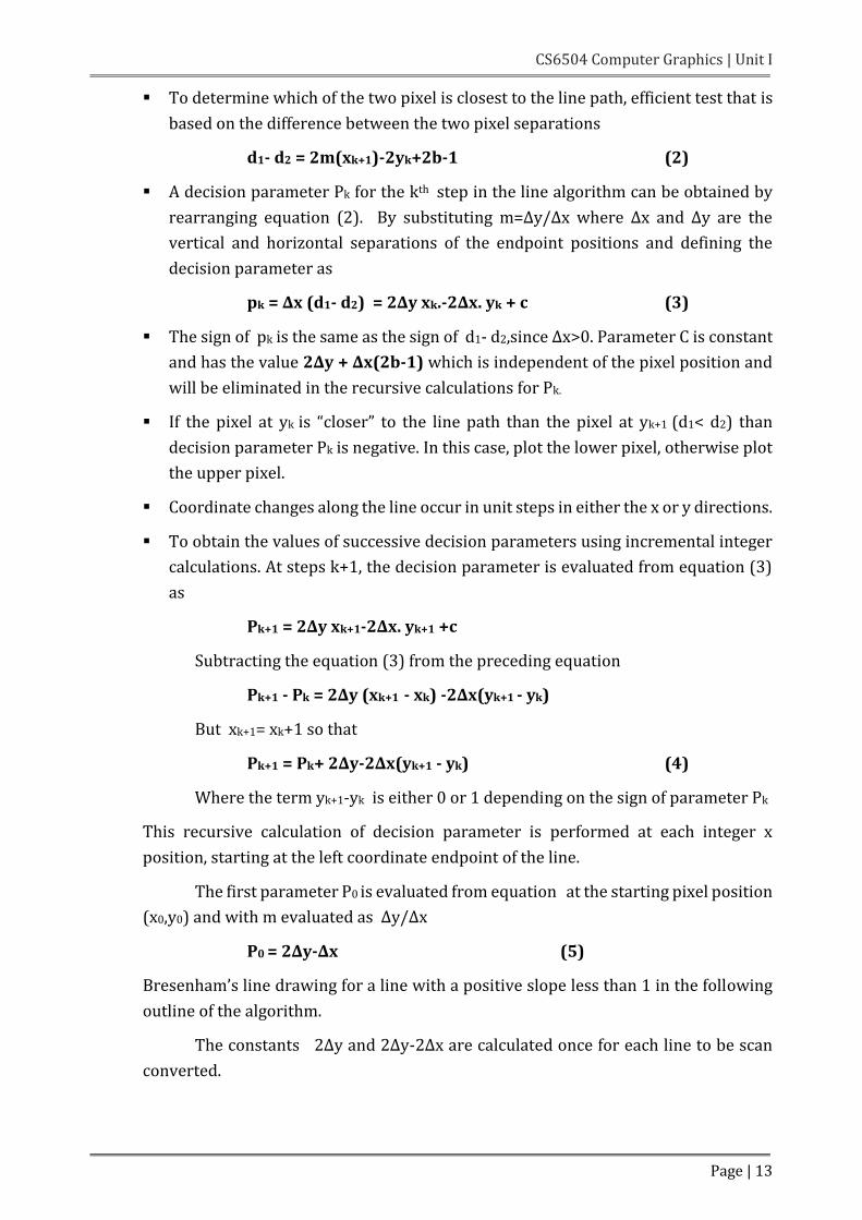
setPixel(x,y);

while(x<xEnd)

{

x++;

if (p<0)

p+=twoDy;

else

{

y++;

p+=twoDyDx;

}

setPixel(x,y);

}

}

Example : Consider the line with endpoints (20,10) to (30,18)

The line has the slope m= (18-10)/(30-20)=8/10=0.8

∆x = 10 ∆y=8

The initial decision parameter has the value

p0 = 2Δy- Δx = 6

and the increments for calculating successive decision parameters are

2Δy=16 2Δy-2 Δx= -4

We plot the initial point (x0,y0) = (20,10) and determine successive pixel positions

along the line path from the decision parameter as

Tabulation

k pk (xk+1, yK+1)

0 6 (21,11)

1 2 (22,12)

2 -2 (23,12)

3 14 (24,13)

4 10 (25,14)

5 6 (26,15)


Page | 16

6 2 (27,16)

7 -2 (28,16)

8 14 (29,17)

9 10 (30,18)

Result

Advantages

Algorithm is Fast

Uses only integer calculations

Disadvantages

It is meant only for basic line drawing.

1.4.3 Line Function

The two dimension line function is Polyline(n,wcPoints) where n is assigned an

integer value equal to the number of coordinate positions to be input and

wcPoints is the array of input world-coordinate values for line segment

endpoints.

polyline function is used to define a set of n – 1 connected straight line segments

To display a single straight-line segment we have to set n=2 and list the and y

values of the two endpoint coordinates in wcPoints.

Example: following statements generate 2 connected line segments with endpoints at

(50, 100), (150, 250), and (250, 100)

typedef struct myPt{int x, y;};

myPt wcPoints[3];

wcPoints[0] .x = 50; wcPoints[0] .y = 100;


Page | 17

wcPoints[1] .x = 150; wcPoints[1].y = 50;

wcPoints[2].x = 250; wcPoints[2] .y = 100;

polyline ( 3 , wcpoints);

1.5 Circle-Generating Algorithms

General function is available in a graphics library for displaying various kinds

of curves, including circles and ellipses.

Properties of a circle

A circle is defined as a set of points that are all the given distance (xc,yc).

This distance relationship is expressed by the pythagorean theorem in Cartesian coordinates as

(x – xc)2 + (y – yc) 2 = r2 (1)

Use above equation to calculate the position of points on a circle circumference by

stepping along the x axis in unit steps from xc-r to xc+r and calculating the

corresponding y values at each position as

y = yc +(- ) (r2 – (xc –x )2)1/2 (2)

This is not the best method for generating a circle for the following reason

o Considerable amount of computation

o Spacing between plotted pixels is not uniform

To eliminate the unequal spacing is to calculate points along the circle boundary using

polar coordinates r and θ. Expressing the circle equation in parametric polar from

yields the pair of equations

x = xc + rcos θ y = yc + rsin θ

When a display is generated with these equations using a fixed angular step size, a

circle is plotted with equally spaced points along the circumference. To reduce

calculations use a large angular separation between points along the circumference

and connect the points with straight line segments to approximate the circular path.


Page | 18

Set the angular step size at 1/r. This plots pixel positions that are

approximately one unit apart. The shape of the circle is similar in each

quadrant.

To determine the curve positions in the first quadrant, to generate he circle

section in the second quadrant of the xy plane by nothing that the two circle

sections are symmetric with respect to the y axis and circle section in the third

and fourth quadrants can be obtained from sections in the first and second

quadrants by considering symmetry between octants.

Circle sections in adjacent octants within one quadrant are symmetric with

respect to the 450 line dividing the two octants. Where a point at position (x, y)

on a one-eight circle sector is mapped into the seven circle points in the other

octants of the xy plane.

To generate all pixel positions around a circle by calculating only the points

within the sector from x=0 to y=0. the slope of the curve in this octant has an

magnitude less than of equal to 1.0. at x=0, the circle slope is 0 and at x=y, the

slope is -1.0.

Bresenham’s line algorithm for raster displays is adapted to circle generation

by setting up decision parameters for finding the closest pixel to the

circumference at each sampling step. Square root evaluations would be

required to computer pixel siatances from a circular path.

Bresenham’s circle algorithm avoids these square root calculations by

comparing the squares of the pixel separation distances. It is possible to

perform a direct distance comparison without a squaring operation.

In this approach is to test the halfway position between two pixels to determine

if this midpoint is inside or outside the circle boundary. This method is more

easily applied to other conics and for an integer circle radius the midpoint

approach generates the same pixel positions as the Bresenham circle

algorithm.


Page | 19

For a straight line segment the midpoint method is equivalent to the

bresenham line algorithm. The error involved in locating pixel positions along

any conic section using the midpoint test is limited to one half the pixel

separations.

1.5.1 Midpoint circle Algorithm:

In the raster line algorithm at unit intervals and determine the closest pixel

position to the specified circle path at each step for a given radius r and screen

center position (xc,yc) set up our algorithm to calculate pixel positions around a

circle path centered at the coordinate position by adding xc to x and yc to y.

To apply the midpoint method we define a circle function as

fcircle(x,y) = x2+y2-r2

Any point (x,y) on the boundary of the circle with radius r satisfies the equation

fcircle (x,y)=0. If the point is in the interior of the circle, the circle function is

negative. And if the point is outside the circle the, circle function is positive

fcircle (x,y) <0, if (x,y) is inside the circle boundary

=0, if (x,y) is on the circle boundary

>0, if (x,y) is outside the circle boundary

The tests in the above eqn are performed for the midposition sbteween pixels near

the circle path at each sampling step. The circle function is the decision parameter

in the midpoint algorithm.

Midpoint between candidate pixels at sampling position xk+1 along a circular path.

Fig -1 shows the midpoint between the two candidate pixels at sampling position

xk+1. To plot the pixel at (xk,yk) next need to determine whether the pixel at position

(xk+1,yk) or the one at position (xk+1,yk-1) is circular to the circle.

Our decision parameter is the circle function evaluated at the midpoint between

these two pixels

Pk = fcircle (xk+1,yk-1/2) = (xk+1)2+(yk-1/2)2-r2

If Pk <0, this midpoint is inside the circle and the pixel on scan line yk is closer to

the circle boundary. Otherwise the mid position is outside or on the circle

boundary and select the pixel on scan line yk -1.

Successive decision parameters are obtained using incremental calculations. To

obtain a recursive expression for the next decision parameter by evaluating the

circle function at sampling position xk+1+1= xk+2

Pk = fcircle (xk+1+1,yk+1-1/2) = [(xk+1)+1]2+(yk+1-1/2)2-r2


Page | 20

or

Pk+1=Pk+2(xk+1)+(y2k+1-y2 k )-(yk+1-yk)+1

Where yk+1 is either yk or yk-1 depending on the sign of Pk .

Increments for obtaining Pk+1 are either 2xk+1+1 (if Pk is negative) or

2xk+1+1-2 yk+1.

Evaluation of the terms 2xk+1 and 2 yk+1 can also be done incrementally as

2xk+1=2xk+2

2 yk+1=2 yk-2

At the Start position (0,r) these two terms have the values 0 and 2r respectively.

Each successive value for the 2xk+1 term is obtained by adding 2 to the previous

value and each successive value for the 2yk+1 term is obtained by subtracting 2

from the previous value.

The initial decision parameter is obtained by evaluating the circle function at the

start position (x0,y0)=(0,r)

P0 = fcircle (1,r-1/2) = 1+(r-1/2)2-r2

or

P0=(5/4)-r

If the radius r is specified as an integer

P0=1-r(for r an integer)

Algorithm: Midpoint circle Algorithm

1. Input radius r and circle center (xc,yc) and obtain the first point on the

circumference of the circle centered on the origin as

(x0,y0) = (0,r)

2. Calculate the initial value of the decision parameter as P0=(5/4)-r

3. At each xk position, starting at k=0, perform the following test. If Pk <0 the next point

along the circle centered on (0,0) is (xk+1,yk) and Pk+1=Pk+2xk+1+1

Otherwise the next point along the circle is (xk+1,yk-1) and Pk+1=Pk+2xk+1+1-2 yk+1

Where 2xk+1=2xk+2 and 2yk+1=2yk-2

4. Determine symmetry points in the other seven octants.

5. Move each calculated pixel position (x,y) onto the circular path centered at (xc,yc)

and plot the coordinate values.

x=x+xc y=y+yc

6. Repeat step 3 through 5 until x>=y.


Page | 21

Example: Midpoint Circle Drawing

Given a circle radius r=10

The circle octant in the first quadrant from x=0 to x=y. The initial value of the decision

parameter is P0=1-r = - 9

For the circle centered on the coordinate origin, the initial point is (x0,y0)=(0,10) and

initial increment terms for calculating the decision parameters are

2x0=0 , 2y0=20

Successive midpoint decision parameter values and the corresponding coordinate

positions along the circle path are listed in the following table.

k pk (xk+1, yk-1) 2xk+1 2yk+1 0 -9 (1,10) 2 20 1 -6 (2,10) 4 20 2 -1 (3,10) 6 20 3 6 (4,9) 8 18 4 -3 (5,9) 10 18 5 8 (6,8) 12 16 6 5 (7,7) 14 14

Implementation of Midpoint Circle Algorithm

void circleMidpoint (int xCenter, int yCenter, int radius)

{

int x = 0, y = radius, p = 1 - radius;

void circlePlotPoints (int, int, int, int);

circlePlotPoints (xCenter, yCenter, x, y);

while (x < y)


Page | 22

{

x++ ;

if (p < 0)

p +=2*x +1;

else

{

y--;

p +=2* (x - Y) + 1;

}

circlePlotPoints(xCenter, yCenter, x, y)

}

}

void circlePlotPolnts (int xCenter, int yCenter, int x, int

y)

{

setpixel (xCenter + x, yCenter + y ) ;

setpixel (xCenter - x. yCenter + y);

setpixel (xCenter + x, yCenter - y);

setpixel (xCenter - x, yCenter - y ) ;

setpixel (xCenter + y, yCenter + x);

setpixel (xCenter - y , yCenter + x);

setpixel (xCenter t y , yCenter - x);

setpixel (xCenter - y , yCenter - x);

}

1.6 Ellipse-Generating Algorithms

An ellipse is an elongated circle. Therefore, elliptical curves can be generated by

modifying circle-drawing procedures to take into account the different dimensions of

an ellipse along the major and minor axes.


Page | 23

Properties of ellipses

An ellipse can be given in terms of the distances from any point on the ellipse to

two fixed positions called the foci of the ellipse. The sum of these two distances is

the same values for all points on the ellipse.

If the distances to the two focus positions from any point p=(x,y) on the ellipse are

labeled d1 and d2, then the general equation of an ellipse can be stated as

d1+d2=constant

Expressing distances d1 and d2 in terms of the focal coordinates F1=(x1,y2) and

F2=(x2,y2)

sqrt((x-x1)2+(y-y1)2)+sqrt((x-x2)2+(y-y2)2)=constant

By squaring this equation isolating the remaining radical and squaring again.

The general ellipse equation in the form

Ax2+By2+Cxy+Dx+Ey+F=0

The coefficients A,B,C,D,E, and F are evaluated in terms of the focal coordinates

and the dimensions of the major and minor axes of the ellipse.

The major axis is the straight line segment extending from one side of the

ellipse to the other through the foci. The minor axis spans the shorter

dimension of the ellipse, perpendicularly bisecting the major axis at the

halfway position (ellipse center) between the two foci.

An interactive method for specifying an ellipse in an arbitrary orientation is to

input the two foci and a point on the ellipse boundary.

Ellipse equations are simplified if the major and minor axes are oriented to

align with the coordinate axes. The major and minor axes oriented parallel to

the x and y axes parameter rx for this example labels the semi major axis and

parameter ry labels the semi minor axis

((x-xc)/rx)2+((y-yc)/ry)2=1


Page | 24

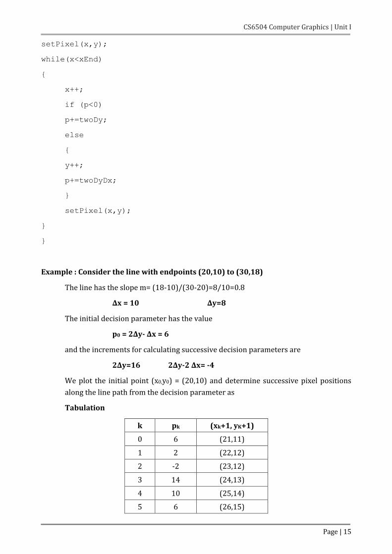
Using polar coordinates r and θ, to describe the ellipse in Standard position

with the parametric equations

x=xc+rxcos θ

y=yc+rxsin θ

Angle θ called the eccentric angle of the ellipse is measured around the

perimeter of a bounding circle.

We must calculate pixel positions along the elliptical arc throughout one

quadrant, and then we obtain positions in the remaining three quadrants by

symmetry

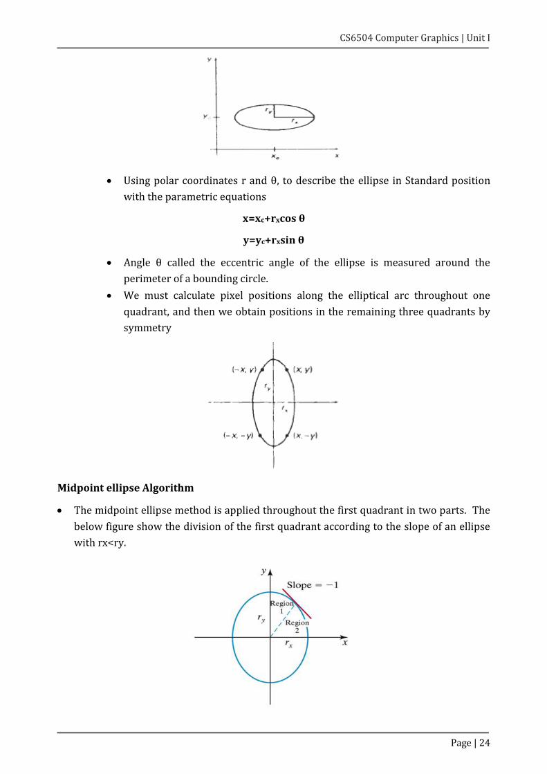
Midpoint ellipse Algorithm

The midpoint ellipse method is applied throughout the first quadrant in two parts. The

below figure show the division of the first quadrant according to the slope of an ellipse

with rx<ry.


Page | 25

In the x direction where the slope of the curve has a magnitude less than 1 and unit

steps in the y direction where the slope has a magnitude greater than 1.

Region 1 and 2 can be processed in various ways

1. Start at position (0,ry) and step clockwise along the elliptical path in the first

quadrant shifting from unit steps in x to unit steps in y when the slope becomes less

than -1

2. Start at (rx,0) and select points in a counter clockwise order.

2.1 Shifting from unit steps in y to unit steps in x when the slope becomes

greater than -1.0

2.2 Using parallel processors calculate pixel positions in the two regions

simultaneously

3. Start at (0,ry)

step along the ellipse path in clockwise order throughout the first quadrant ellipse

function (xc,yc)=(0,0)

fellipse (x,y)=ry2x2+rx2y2 –rx2 ry2

which has the following properties:

fellipse (x,y) <0, if (x,y) is inside the ellipse boundary

=0, if(x,y) is on ellipse boundary

>0, if(x,y) is outside the ellipse boundary

Thus, the ellipse function fellipse (x,y) serves as the decision parameter in the midpoint

algorithm.

Starting at (0,ry):

Unit steps in the x direction until to reach the boundary between region 1 and region

2. Then switch to unit steps in the y direction over the remainder of the curve in the first

quadrant.

At each step to test the value of the slope of the curve. The ellipse slope is calculated

dy/dx= -(2ry2x/2rx2y)

At the boundary between region 1 an region 2

dy/dx = -1.0 and 2ry2x=2rx2y

to more out of region 1 whenever

2ry2x>=2rx2y


Page | 26

The following figure shows the midpoint between two candidate pixels at sampling

position xk+1 in the first region.

To determine the next position along the ellipse path by evaluating the decision

parameter at this mid point

P1k = fellipse (xk+1,yk-1/2)

= ry2 (xk+1)2 + rx2 (yk-1/2)2 – rx2 ry2

if P1k <0, the midpoint is inside the ellipse and the pixel on scan line yk is closer

to the ellipse boundary. Otherwise the midpoint is outside or on the ellipse

boundary and select the pixel on scan line yk-1

At the next sampling position (xk+1+1=xk+2) the decision parameter for region 1 is

calculated as

p1k+1 = fellipse(xk+1 +1,yk+1 -½ )

=ry2[(xk +1) + 1]2 + rx2 (yk+1 -½)2 - rx2 ry2

Or

p1k+1 = p1k +2 ry2(xk +1) + ry2 + rx2 [(yk+1 -½)2 - (yk -½)2]

Where yk+1 is yk or yk-1 depending on the sign of P1k.

Decision parameters are incremented by the following amounts

increment = { 2 ry2(xk +1) + ry2 if p1k <0 }

{ 2 ry2(xk +1) + ry2 - 2rx2 yk+1 if p1k ≥ 0 }

Increments for the decision parameters can be calculated using only addition and

subtraction as in the circle algorithm.

The terms 2ry2 x and 2rx2 y can be obtained incrementally. At the initial position

(0,ry) these two terms evaluate to

2 ry2x = 0


Page | 27

2rx2 y =2rx2 ry

x and y are incremented updated values are obtained by adding 2ry2to the

current value of the increment term and subtracting 2rx2 from the current

value of the increment term. The updated increment values are compared at

each step and more from region 1 to region 2. when the condition 4 is satisfied.

In region 1 the initial value of the decision parameter is obtained by evaluating

the ellipse function at the start position

(x0,y0) = (0,ry)

region 2 at unit intervals in the negative y direction and the midpoint is now

taken between horizontal pixels at each step for this region the decision

parameter is evaluated as

p10 = fellipse(1,ry -½ )

= ry2 + rx2 (ry -½)2 - rx2 ry2

Or

p10 = ry2 - rx2 ry + ¼ rx2

over region 2, we sample at unit steps in the negative y direction and the

midpoint is now taken between horizontal pixels at each step. For this region,

the decision parameter is evaluated as

p2k = fellipse(xk +½ ,yk - 1)

= ry2 (xk +½ )2 + rx2 (yk - 1)2 - rx2 ry2

1. If P2k >0,

the midpoint position is outside the ellipse boundary, and select the pixel at xk.

2. If P2k <=0,

the midpoint is inside the ellipse boundary and select pixel position xk+1.

To determine the relationship between successive decision parameters in region

2 evaluate the ellipse function at the sampling step : yk+1 -1= yk-2.

P2k+1 = fellipse(xk+1 +½,yk+1 -1 )

=ry2(xk +½) 2 + rx2 [(yk+1 -1) -1]2 - rx2 ry2

or

p2k+1 = p2k -2 rx2(yk -1) + rx2 + ry2 [(xk+1 +½)2 - (xk +½)2]


Page | 28

With xk+1set either to xkor xk+1, depending on the sign of P2k. when we enter region

2, the initial position (x0,y0) is taken as the last position. Selected in region 1 and

the initial decision parameter in region 2 is then

p20 = fellipse(x0 +½ ,y0 - 1) = ry2 (x0 +½ )2 + rx2 (y0 - 1)2 - rx2 ry2

To simplify the calculation of P20, select pixel positions in counter clock wise order

starting at (rx,0). Unit steps would then be taken in the positive y direction up to

the last position selected in region 1.

Algorithm: Midpoint Ellipse Algorithm

1. Input rx,ry and ellipse center (xc,yc) and obtain the first point on an ellipse

centered on the origin as

(x0,y0) = (0,ry)

2. Calculate the initial value of the decision parameter in region 1 as

P10=ry2-rx2ry +(1/4)rx2

3. At each xk position in region1 starting at k=0 perform the following test. If P1k<0,

the next point along the ellipse centered on (0,0) is (xk+1, yk) and

p1k+1 = p1k +2 ry2xk +1 + ry2

Otherwise the next point along the ellipse is (xk+1, yk-1) and

p1k+1 = p1k +2 ry2xk +1 - 2rx2 yk+1 + ry2

with

2 ry2xk +1 = 2 ry2xk + 2ry2

2 rx2yk +1 = 2 rx2yk + 2rx2

And continue until 2ry2 x>=2rx2 y

4. Calculate the initial value of the decision parameter in region 2 using the last

point (x0,y0) is the last position calculated in region 1.

p20 = ry2(x0+1/2)2+rx2(yo-1)2 – rx2ry2

5. At each position yk in region 2, starting at k=0 perform the following test, If

p2k>0 the next point along the ellipse centered on (0,0) is (xk,yk-1) and

p2k+1 = p2k – 2rx2yk+1+rx2

Otherwise the next point along the ellipse is (xk+1,yk-1) and

p2k+1 = p2k + 2ry2xk+1 – 2rx2yk+1 + rx2

Using the same incremental calculations for x any y as in region 1.

6. Determine symmetry points in the other three quadrants.


Page | 29

7. Move each calculate pixel position (x,y) onto the elliptical path centered on (xc,yc)

and plot the coordinate values

x=x+xc, y=y+yc

8. Repeat the steps for region1 unit 2ry2x>=2rx2y

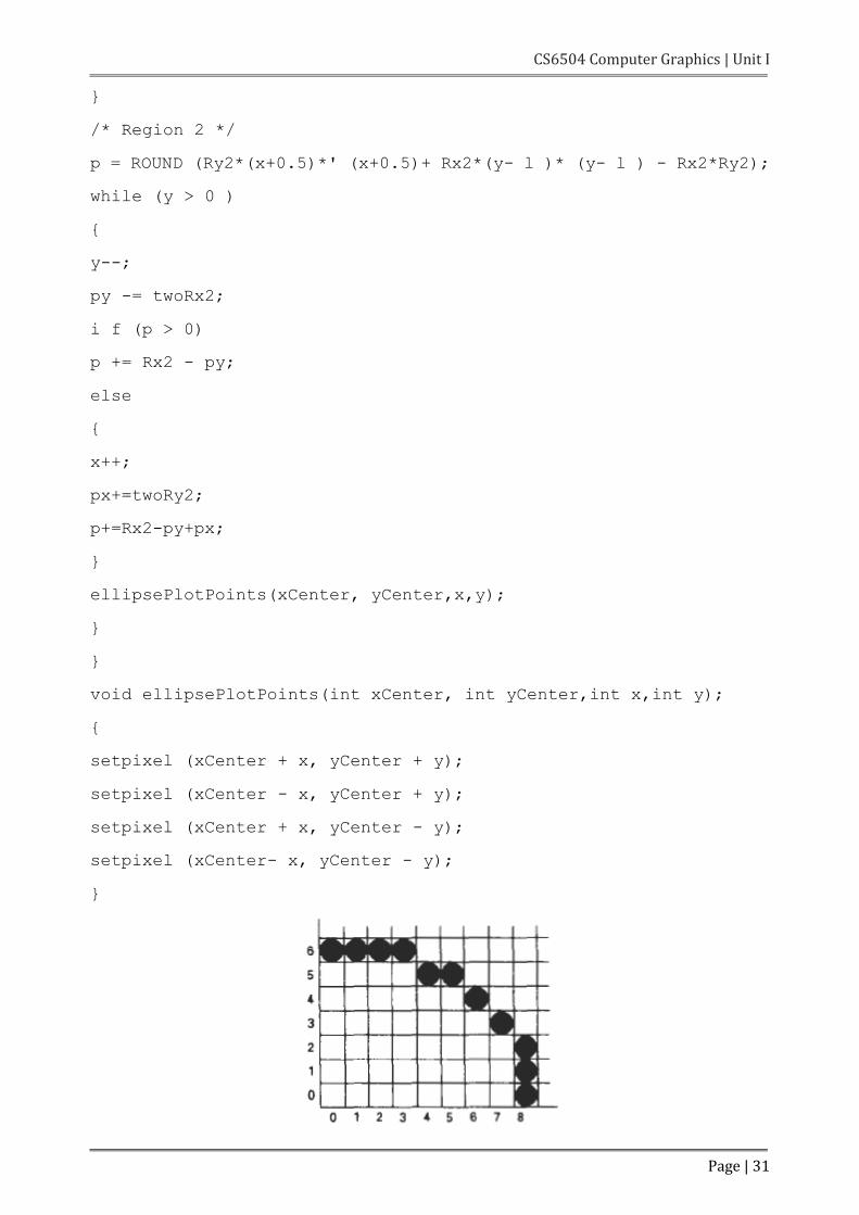
Example : Mid point ellipse drawing

Input ellipse parameters rx=8 and ry=6 the mid point ellipse algorithm by determining

raster position along the ellipse path is the first quadrant. Initial values and increments for

the decision parameter calculations are

2ry2 x=0 (with increment 2ry2=72 )

2rx2 y=2rx2 ry (with increment -2rx2= -128 )

For region 1 the initial point for the ellipse centered on the origin is (x0,y0) = (0,6) and the

initial decision parameter value is

p10=ry2-rx2ry2+1/4rx2=-332

Successive midpoint decision parameter values and the pixel positions along the ellipse are

listed in the following table.

K p1k xk+1,yk+1 2ry2xk+1 2rx2yk+1

0 -332 (1,6) 72 768

1 -224 (2,6) 144 768

2 -44 (3,6) 216 768

3 208 (4,5) 288 640

4 -108 (5,5) 360 640

5 288 (6,4) 432 512

6 244 (7,3) 504 384

Move out of region 1, 2ry2x >2rx2y .

For a region 2 the initial point is (x0,y0)=(7,3) and the initial decision parameter is

p20 = fellipse(7+1/2,2) = -151

The remaining positions along the ellipse path in the first quadrant are then

calculated as

K P2k xk+1,yk+1 2ry2xk+1 2rx2yk+1

0 -151 (8,2) 576 256

1 233 (8,1) 576 128

2 745 (8,0) - -


Page | 30

Implementation of Midpoint Ellipse drawing

#define Round(a) ((int)(a+0.5))

void ellipseMidpoint (int xCenter, int yCenter, int Rx, int Ry)

{

int Rx2=Rx*Rx;

int Ry2=Ry*Ry;

int twoRx2 = 2*Rx2;

int twoRy2 = 2*Ry2;

int p;

int x = 0;

int y = Ry;

int px = 0;

int py = twoRx2* y;

void ellipsePlotPoints ( int , int , int , int ) ;

/* Plot the first set of points */

ellipsePlotPoints (xcenter, yCenter, x,y ) ;

/ * Region 1 */

p = ROUND(Ry2 - (Rx2* Ry) + (0.25*Rx2));

while (px < py)

{

x++;

px += twoRy2;

i f (p < 0)

p += Ry2 + px;

else

{

y - - ;

py -= twoRx2;

p += Ry2 + px - py;

}

ellipsePlotPoints(xCenter, yCenter,x,y);


Page | 31

}

/* Region 2 */

p = ROUND (Ry2*(x+0.5)*' (x+0.5)+ Rx2*(y- l )* (y- l ) - Rx2*Ry2);

while (y > 0 )

{

y--;

py -= twoRx2;

i f (p > 0)

p += Rx2 - py;

else

{

x++;

px+=twoRy2;

p+=Rx2-py+px;

}

ellipsePlotPoints(xCenter, yCenter,x,y);

}

}

void ellipsePlotPoints(int xCenter, int yCenter,int x,int y);

{

setpixel (xCenter + x, yCenter + y);

setpixel (xCenter - x, yCenter + y);

setpixel (xCenter + x, yCenter - y);

setpixel (xCenter- x, yCenter - y);

}


Page | 32

1.6 Pixel Addressing and Object Geometry

There are two ways to adjust the dimensions of displayed objects in finite pixel areas,

1. The dimensions of displayed objects are adjusted according to the amount

of overlap of pixel areas with the object boundaries

2. We align object boundaries with pixel boundaries instead of pixel centers.

Advantages of pixel-addressing scheme:

1. It avoids half-integer pixel boundaries

2. It facilitates precise object representations

3. It simplifies the processing involved in many scan-conversion algorithms

and in other raster procedures.

Maintaining Geometric: Properties of displayed objects

When we convert geometric descriptions of objects into pixel representations, we

transform mathematical points and lines into finite screen areas.

During this transformation, if we are to maintain the original geometric

measurements specified by the geometric descriptions for an object, we need to

consider the finite size of pixels.

1.6.1 Antialiasing and Antialiasing Techniques

In the line drawing algorithms, we have seen that all rasterized locations do not

match with the true line and we have to select the optimum raster locations to

represent a straight line.

This problem is severe in low resolution screens. In such screen, line appears like

a stair-step. This effect is known as Aliasing. It is dominant for lines having gentle

and sharp slopes.

Antialiasing:

The aliasing effect can be reduced by adjusting intensities of the pixels along the

line. The process of adjusting intensities of the pixels along the line to minimize

the effect of aliasing is called antialiasing.

The aliasing effect can be reduced by increasing resolution of the raster display.

With raster systems that are capable of displaying more than two intensity levels,

we can apply antialiasing methods to modify pixel intensities.

Antialiasing methods are basically classified as,

1. Supersampling or Postfiltering

2. Area Sampling or Prefiltering

3. Filtering Techniques

4. Pixel Phasing


Page | 33

1.7 Filled Area Primitives

Introduction

A Ployline is a chain of connected line segments.

It is specified by giving the verties(nodes) P0, P1, P2,… and so on.

The first vertex is called the initial or starting point and the last vetex is known as

the final or terminal point.

When starting point and terminal point of any polyline is same, then it is known

as polygon.

Ployline Polygon

Types of Ploygons

The classification of polygons is based on where the line segment joining any two

points within the polygon is going to be:

1. Convex Polygon

A Convex Ploygon is a polygon in which the line segment joining any

two points within the polygon lies completely inside the polygon.

2. Concave Plygon

A Convex Ploygon is a polygon in which the line segment joining any two

points within the polygon may not lie completely inside the polygon.


Page | 34

Representation of Polygons

There are three approaches to represent polygons according to the graphics

systems:

1. Ploygon drawing primitive approach

2. Trapezoid primitive approach

3. Line and point approach

Some graphics devices supports polygon drawing primitive approach and they

can directly draw the polygon shapes.

Some devices support trapezoid primitives. In such devices, trapezoid is formed

when two scan lines and two line segments.

Ploygon Ploygon as a series of trapezoids

Most of the devices do not provide any polygon support at all. In such devices

polygons are represented using lines and points.

A polygon is represented as a unit and it is stored in the display file.

Ploygon Algorithm:

1. Read AX and AY of length N

[AX and AY are arrays containing the vertices of the polygon and N is the number

of polygon sides]

2. i = 0 [Initialize counter to count number of sides]

DF_OP [ i ] = N

DF_x [ i ] = AX [ i ]

DF_y [ i ] = AY [ i ]

i = i + 1


Page | 35

3. do

{

DF_OP [ i ] = 2

DF_x [ i ] = AX [ i ]

DF_y [ i ] = AY [ i ]

i = i + 1

} while (i<N)

4. DF_OP [ i ] = 2

DF_x [ i ] = AX [ 0 ]

DF_y [ i ] = AY [ 0 ]

5. Stop

Ploygon Filling

Fille the polygon means highlighting all pixels which lie inside the polygon with

any colour other than background colour.

Ploygons are easier to fill since they have linear boundaries. There are two basic

approaches to fill the polygon such as,

1. Seed Fill Algorithm

One way to fill a polygon is to start from a given ‘seed; point known

to be inside the polygon and highlight outward from this point that

is neighbouring pixels until we encounter the boundary pixels.

This approach is known as seed fill because colour flows from the

sead point until reaching the polygon boundary, like water flooding

on the surface of the container.

The seed fill algorithm is further classified as Flood Fill Algorithm

and Boundary Fill Algorithm.

Algorithms that fill interior-defined regions are called flood-fill

algorithms. Those that fill boundary-defined regions are called

boundary-fill algorithms or edge-fill algorithms.


Page | 36

2. Scan-Line Algorithm

In this approach, inside test will be applied to check whether the

pixel is inside the polygon or outside the polygon and then highlight

pixels which lie inside the polygon.

This approach is known as scan-line algorithm. It avoids the need

for a seed pixel but it requires some computation.

This algorithm solves the hidden surface problem while generating

display scan line.

It is used in orthogonal projection and it is non-recursive algorithm.

In scan line algorithm, we have to stack only a beginning position for

each horizontal pixel scan, instead of stacking all unprocessed

neighbouring positions around the current position.

PART-A

1. Define Computer graphics.

2. What are the video display devices

3. Define refresh buffer/frame buffer.

4. What is meant by scan code?

5. List out the merits and demerits of Penetration techniques?

6. List out the merits and demerits of DVST

7. What do you mean by emissive and non-emissive displays

8. List out the merits and demerits of Plasma panel display

9. What is raster scan and Random scan systems

10. What is pixel?

11. What are the Input devices and Hard copy devices?

12. Define aspect ratio.

13. What is Output Primitive? What is point and lines in the computer graphics system?

14. What is DDA? What are the disadvantages of DDA algorithm?

15. Digitize a line from (10,12) to (15,15) on a raster screen using Bresenhams straight line

Algorithm what are the various line drawing algorithms

16. What is loading a frame buffer?


Page | 37

17. What is meant by antialiasing?

18. What is a filled area primitive?

19. What are the various for the Filled area Primitives

20. What is pixel addressing and object addressing

PART-B

1. Explain the following Video Displays Devices (a) refresh cathode ray tube(b)raster Scan

Displays (c) Random Scan Displays (d)Color SRT Monitors

2. Explain Direct View Storage Tubes(b) Flat Panel Displays (c)Liquid Crystal Displays

3. Explain Raster scan systems and Raster Scan Systems

4. Explain the Various Input Devices

5. Explain (a) Hard Copy devices(b)Graphics Software

6. Explain in detail about the Line drawing DDA scan conversion algorithm?

7. Write down and explain the midpoint circle drawing algorithm. Assume 10 cm as the radius

and co-ordinate as the centre of the circle.

8. Calculate the pixel location approximating the first octant of a circle having centre at (4,5)

and radius 4 units using Bresenham’s algorithm

9. Explain Ellipse generating Algorithm?

10. Explain Boundary Fill Algorithm?

unit i introduction - google search

Documents