unit 7: minimizing costs and maximizing …personal.unizar.es/jamolina/_/microeconomia/unit...

UNIT 7: MINIMIZING COSTS AND MAXIMIZING PROFITS

J. Alberto Molina – J. I. Giménez Nadal

UNIT 7: MINIMIZING COSTS AND MAXIMIZING PROFITS

1. Minimizing costs

2. Conditional factor demands

3. Cost functions

4. Long‐run and short‐run costs

5. Marginal income, marginal cost and maximizingprofits

Unit 7 – Pg. 1

Unit 6: How to produce…– Technically efficient combination of factors

Unit 7: …at the minimum cost?– Combination of production factors that, at given prices, lead to the

minimum cost

Example: Productive processes that are technically efficient, aimed at producing 10 units of output. Prices of production factors: w=1, r=3

Process Labour (L) Capital (K) Output Cost= w·L+r·KA 2 3 10 11 = 1·2+3·3B 3 2 10 9 = 1·3+3·2D 1 4 10 13 = 1·1+3·4

The production process B is economically efficient: it allows a given amountof output at the minimum cost.

1. MINIMIZING COSTS

Unit 7 – Pg. 2

The firm’s goal is maximization of profits, determining theamount of output (q) and the necessary quantities of inputs (Land K). In doing so, the firm proceeds in 2 steps:

1. Cost‐minimization

The optimum quantity of Labour (L*) and capital (K*), subjectto a given amount of output, are determined, as well as the costfunction.

2. Profit‐maximization

Following the previous step, the optimum quantity of output(q*) is determined.

1. MINIMIZING COSTS

Unit 7 – Pg. 3

We analyze the cost minimization by the firm from a long‐run pespective. Thatis, considering that all the productive factors are variable (freely eligible)

Knowing the production function q=f(L,K), which covers all the productionprocesses that are technically efficient, we assume that the firm combines labour and capital to produce a given amount of output q0.

Given the prices of labour (w=w0) and capital (r=r0), the production cost of each combination of productive factors (L,K) is given by:

C = w0 ∙ L + r0 ∙ KThe firm aims to produce the amount of output q0 by choosing thecombination of inputs that minimizes the production cost (economicallyefficient):

0 0

L,K 0min C w L r Ks.t. q f(L,K)

1. MINIMIZING COSTS

Unit 7 – Pg. 4

We can represent graphically the solution of the cost‐minimization problem:The objective function of the problem of cost minimization can be

represented with the map of isocost lines(Isocost line: set of combinations of productive factors that, given w0 and r0

leads to the same production cost):

Lrw

rCKKrLwC 0

0

0

0000

)tg(rw

dLdK

0

0

CC 0

This is a linear equation, whoseslope measures the substitutionrate between labour and capital, sothat the cost is constant:

1. MINIMIZING COSTS

Unit 7 – Pg. 5

• Prices of productive factors • Cost level

1 01

0

w (w w )wsloper

1 00

0

C (C C )wsloper

1. MINIMIZING COSTS

Unit 7 – Pg. 6

Map of isocost lines: given the prices of the productive factors (w0 and r0), we consider all the posible costs of production for the firm. There is a different

isocost line for each combination of productive factors:

012 CCC

)tg(rw0

0

1. MINIMIZING COSTS

Unit 7 – Pg. 7

The constraint of the problem of cost‐minimization by the firm is the isoquantcurve corresponding to the production level q0. That is to say, all thecombinations of labour and capital that are technically efficient to obtain q0

1. MINIMIZING COSTS

Unit 7 – Pg. 8

B

L*

K*

A

L

K

qº

E

Given the production function, the isoquant curve of level q0 represents all thecombinations of inputs that are technically efficient.

If we know the prices of the productive factors, w0 and r0, producing q0 at point A meansthat the isocost line that crosses at point A has a slope measured by the relative price: tg=w0/r0

Producing q0 at point B means a lower cost compared to point A. There is an isocost line thatcrosses at point B and is closer to the origin.

The combination E=(L*, K*) minimizes the cost of producing q0

at the relative price tg

E is the tangent point between the isoquant of level q0 and the isocost line with slope tg

For any absolute prices of the productivefactors, if the relative price is tg thenE=(L*,K*) will always be the combination thatminimizes the cost of producing q0

1. MINIMIZING COSTS

Unit 7 – Pg. 9

The isocost line that is closest to the origin is tangent to the isoquantcorresponding to q0 : their slopes are equal at the combination of inputs that minimize the cost (L*,K*)

Slope of the isoquant:

Slope of the isocost:

At minimum cost, that is to say, at the equilibrium (L*, K*):

Tangency condition:

Production restriction:

0

KL

q q

f (L,K)dK RTS (L,K)dL f (L,K)

L

K

M

0

0

CC rw

dLdK

0

* *KL * *

f (L ,K ) wºMRTS (L*,K*)f (L ,K ) rº

º ( *, *)

L

Kq f L K

1. MINIMIZING COSTS

Unit 7 – Pg. 10

Analytically, the problem of cost‐minimization consists,of solving the followingconditioned optimization problem:

0 0

L,K 0min C w L r Ks.t. q f(L,K)

K)f(L,qμKrLwμ)K,(L, 000

where:• Endogenous variables: L y K• Exogenous variables: w0, r0 y q0

To solve this problem, we need to formulate the following Lagrangian:

and, consequently, the problem becomes:

μ)K,(L,minμK,L,

1. MINIMIZING COSTS

Unit 7 – Pg. 11

The first‐order conditions (FOCs) form a system of 3 equations with 3 unknown quantities(L,K,µ):

K)f(L,q0K)f(L,q0μ

fμr0Kfμr0

K

fμw0Lfμw0

L

00μ

K00

K

L00

L

The second‐order condition (SOC) is automatically fulfilled under the strictconvexity of the isoquant curves

K)f(L,qμKrLwμ)K,(L, 000 Min

1. MINIMIZING COSTS

Unit 7 – Pg. 12

Using the first two FOCs we can formulate the Law of Equality of the WeightedMarginal Productivity (LEWMP), equivalent to the tangency condition beweenthe isocost line and the isoquant curve:

K * * LL

K

f wºRTS (L , K )f rº

M

)K,L(K)f(L,qrw

ff

**

0

0

0

K

L

The firm minimizes its cost when the additional output generated by the last monetaryunit spent on each input is the same. From the LEWMP and the expression of the isoquant curve of level qº we obtain thesolution to the problem of cost‐minimization: given the prices, the quantities of labour(L*) and capital (K*) that must be used to produce q0 at the minimum cost:

L Kf fLEWMP:wº rº

1. MINIMIZING COSTS

We can then determine the lowest cost of producing q0 at the given prices:

C*=wº.L* + rº. K*

Unit 7 – Pg. 13

For each pair of input prices, the economically efficient combination to produce q0 is unique

Lº

Kº

L

K

qº

Eº

L’

K’

Given the production function, the isoquant curve of level q0 contains all theinput combinations that are technically efficient to produce q0

The combination E0 =(L0, K0) minimizes the cost of producing qº at the relative price tg

E’

The combination E’=(L’, K’) minimizes the cost of producing q0 at the relative price tg

E’’The combination E’’=(L’’, K’’) minimizes the cost of producing qºat the relative price tg

L’’

K’’

1. MINIMIZING COSTS

Unit 7 – Pg. 14

L,Kmin C w L r Ks.t. q f(L,K)

q)r,K(w,Kq)r,L(w,L

We can formulate the problem of cost-minimization without giving specific values to the exogenous variables (w,r,q):

Applying the usual solution method, we obtain the Conditional Factor Demands(CFDs):

that determine the quantities of labour and capital needed to obtain, at any given prices, a specific level of production at the minimum cost.

2. CONDITIONAL FACTOR DEMANDS

Unit 7 – Pg. 15

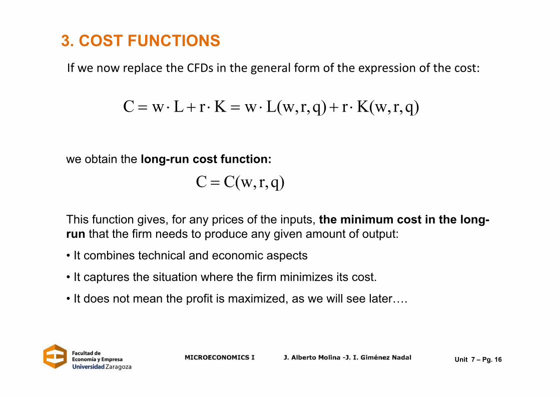
If we now replace the CFDs in the general form of the expression of the cost:

q)r,K(w,rq)r,L(w,wKrLwC

q)r,C(w,C we obtain the long-run cost function:

This function gives, for any prices of the inputs, the minimum cost in the long-run that the firm needs to produce any given amount of output:

• It combines technical and economic aspects

• It captures the situation where the firm minimizes its cost.

• It does not mean the profit is maximized, as we will see later….

3. COST FUNCTIONS

Unit 7 – Pg. 16

Some properties of the cost function in the long‐run:

1. It is increasing with the price of the inputs (w y r)– If the price of any of the inputs increases, the firm will have a higher

cost to produce the same amount of output

2. It is increasing with the quantity of output (q), for given prices of the inputs– Given w and r, a higher quantity of output can be produced only if the

firm assumes a higher cost.

3. It is homogeneous of degree 1 in the input prices

q)r,C(w,C

q)r,C(w,λq)r,λw,C(λ :0λq,w,r,

3. COST FUNCTIONS

Unit 7 – Pg. 17

Taking the conditional factor demands (CFD) L=L(w,r,q), K=K(w,r,q), weobtain the cost function in the long-run C=C(w,r,q) and, if we know theprice of the inputs (w=w0,r=r0), we will obtain the Conditional Factor Demands at the given prices:

Then, we can obtain the cost function in the long‐run:

The cost function in the long-run measures, for any given prices of inputs, the

minimum cost that is needed to produce any amount of output in the long-run

(when L and K are considered to be variable).

(q)LCC

L(q)L K(q)K

3. COST FUNCTIONS

Unit 7 – Pg. 18

The EXPANSION PATH connects optimal input combinations as the scale of production expands. It is a line that connects the combination of inputs that minimize the cost of producing eachamount of output at the given relative prices.

L’Lº

K’’

Kº

L

K

qº

q’’

q’

K’

L’’

EP(tg)

Given the production function and the relative price tg, for each amountof output, the combination of inputs that minimizes the cost is determined

Combination of inputs where:

( , )KL

wMRTS L K tg

r

3. COST FUNCTIONS

Unit 7 – Pg. 19

We obtain the COST CURVE in the long‐run thatassigns, to each level of output, the minimumcost to produce it, at the given prices of theinputs

L’Lº

K’’

Kº

L

K

qº

q’’

q’

K’

L’’

TE(tg)

qqº q’’q’

C

CºC’

C’’

Given the production function and the price of the inputs, theexpansion path can be determined as follows:

3. COST FUNCTIONS

Unit 7 – Pg. 20

Considering the cost function in the long‐run, we can define:

Average cost: cost per unit of produced output

– It is the slope of the vector which links each point of the cost curve in the long‐run to the origin

– It reaches its optimum (minimum) when the vector is tangent to the curve

– Minimum Efficient Scale (qMES): amount of output that minimizes the averagecost

Marginal cost: the change in cost when the output changes by one unit:

– It measures the slope of the cost curve in the long‐run

– It reaches its minimum at the inflexion point

CL(q)AC (q)qL

Δq 0L L

LΔC (q) dC (q)MC (q)Δq dq

3. COST FUNCTIONS

Unit 7 – Pg. 21

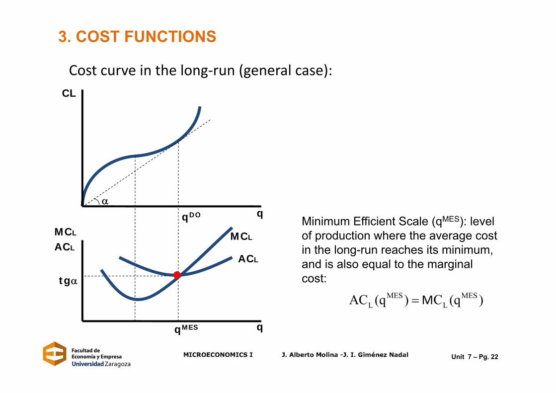
Cost curve in the long‐run (general case):

q

CL

qDO

tg

MCL MCL

q

Minimum Efficient Scale (qMES): level of production where the average cost in the long-run reaches its minimum, and is also equal to the marginal cost:

MES MESL LAC (q ) C (q )M

ACL

qMES

ACL

3. COST FUNCTIONS

Unit 7 – Pg. 22

q

CL

CL(qº)

ACL(qº)

qqº

LL

C (qº)AC (qº)qº

The total cost of producing q0 is the area of base q0 and height ACL(q0):

L LC (qº) C (qº) qºA

3. COST FUNCTIONS

MCL

ACL

MCL

ACL

Unit 7 – Pg. 23

q

CL

CL(qº)

MCL

ACLMCL

q

AML

qº

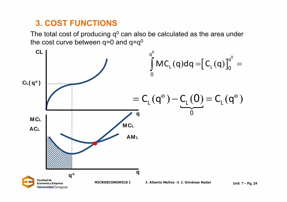
The total cost of producing q0 can also be calculated as the area under the cost curve between q=0 and q=q0

( ) ( )q

qL LMC q dq C q

00

00

( º ) ( ) ( º )L L LC q C C q 0

0

3. COST FUNCTIONS

Unit 7 – Pg. 24

If there are technological improvements, with the same quantities of inputs, the firm will obtain a higher amount of output (to produce any amount of output the firm will need fewer units of inputs) ⇒ the production function changes ⇒ the isoquant map changes ⇒ the MRTS changes ⇒ the Expansion Path changes ⇒ the cost function changes:

3. COST FUNCTIONS

a a a a

L

K

EP (Initial technology)

EP (after the technological change)

qºqº

q’ q’

Now any amount of output can be produced with fewer units of inputs

and hence with a lower cost

Unit 7 – Pg. 25

If there is a change in the relative price of the inputs ⇒ the Expansion Path changes ⇒ the cost function changes:

3. COST FUNCTIONS

a

Lº

Kº

L

K

qº

q’’

q’

b

With the same cost needed to produce qº, now q’ can be produced

a

L’Lº L

K

qº

q’’

q’

b b

K’

To produce qº with minimum cost, (L’,K’) must be used now, leading to a lower cost

Unit 7 – Pg. 26

Technical improvement or decrease in the price of any of the inputs ⇒ the cost function moves downwards:

3. COST FUNCTIONS

Unit 7 – Pg. 27

The form of the cost curves is related to the type of returns to scale of theproduction function:

1. If the technology has constant returns to scale:0 1

0 1L L1 0 1 0

L L

q f(L,K) q f(λ L,λ K)C w L r K C w λ L r λ Kso that q λ q , and thus C λ C

ACL

MCL

MCL=ACL

3. COST FUNCTIONS

Unit 7 – Pg. 28

2. If the technology presents increasing returns to scale:

0 10 1

L L1 0 1 0L L

q f(L,K) q f(λ L,λ K)C w L r K C w λ L r λ Kso that q λ q , and thus C λ C

ACL

MCL

ACL

MCL

3. COST FUNCTIONS

Unit 7 – Pg. 29

3. In the case that the technology presents decreasing returns to scale:

0 10 1

L L1 0 1 0L L

q f(L,K) q f(λ L,λ K)C w L r K C w λ L r λ Kso that q λ q ,and thus C λ C

ACL

MCL

ACL

MCL

3. COST FUNCTIONS

Unit 7 – Pg. 30

We have analyzed the problem of cost‐minimization, considering thatall the productive factors are variable (long‐run). We have obtainedthe Conditioned Factor Demands (CFD) and the cost function in thelong‐run.

We now suppose we are in the short‐run. That is, we also want to minimize the production cost, but now we assume that the firm has a certain quantity of capital (fixed factor) available, and that the firmcannot modify it, and thus the firm is able to decide only the amountof labour (variable factor). We formulate the problem as follows:

Lmin C w L r Ks.t. q f(L,K)

4. LONG-RUN AND SHORT-RUN COSTS

Unit 7 – Pg. 31

L’Lº L

K

qº

q’’

q’

Kº

L’’

Given the production functionand the size of the firm: Kº,

for each amount of output, the firm can determine the unique technically efficient combination of inputs that allows it to produce the given amount of output

for any given relative price, it will be the chosen combination, and the isocost line related to this combination will measure the minimum cost in the short-run with a firm size of Kº:

and, given that it is unique,


Unit 7 – Pg. 32

L’Lº L

K

qº

q’’

q’

Kº

L’’

Given the production function, the size of the firm: Kº and the input prices wº, rº (wº/rº=tg

To each output, we associate the cost in the short-run of producing it for a firm of size Kº :

For any output the firm wants to produce, its cost in the short run is Cc=CFº+ CV(q)

For any given amount of output (even if the firm does not produce), the firm always incurs the fixed cost: FCº= wº.Kº

qqº q’’q’

CT

CºC’

C’’

CFº

4. LONG‐RUN AND SHORT‐RUN COSTS

Unit 7 – Pg. 33

L’Lº L

K

qº

q’’

q’

Kº

L’’

We obtain the COST CURVE IN THE SHORT-RUN, that links to each amount of output the minimum cost of production for a firm of size Kº, at the given prices of the inputs

qqº q’’q’

CT

CºC’

C’’

CFº

Given the production function, the size of the firm: Kº and the input prices wº, rº (wº/rº=tg

To each output we associate the cost in the short-run of producing it for a firm of size Kº:


Unit 7 – Pg. 34

Analytically, under this framework of short‐run, from the production functionthe conditioned demand of the variable input can be determined:

)KL(q,L)Kf(L,qK)f(L,qKK

)Kq,r,CT(w,Kr)KL(q,wCT

If we substitute the conditioned demand in the expression of the cost, we obtain the cost function in the short-run:

•It is increasing in the price of the inputs and the amount of output

TC(q) VC(q) FC and, given the input prices, the cost curve in the short-run can be obtained:

where:

• TC is the total cost (depends on the level of production)

• VC is the variable cost (depends on the level of production)

• Fc is the fixed cost (does not depend on the level of production)


Unit 7 – Pg. 35

It can be shown that, given the law of diminishing marginal returns, the cost curve in the short run goes from concave to convex:

q

TCVCFC

FC

VC

TC=VC+FC

FC


Unit 7 – Pg. 36

VC(q)AVC(q)q

TC(q) VC(q) FCATC(q)q q q

d VC(q) FCdTC(q) dVC(q)MC(q)dq dq dq

MAVC MAVCMC(q ) (q )AVC

MC(q ) TC(q )MATC MATCA

Minimum average variable cost (qMAVC): amount of output that minimizes the average variable cost:

Minimum average total cost (qMATC): amount of output that minimizes the average total cost:

q

CT

q

MCAC

ATC

MCqME

tg

AVCtg

qOE

FC

qME qOE


Unit 7 – Pg. 37

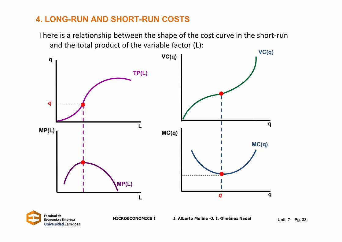
There is a relationship between the shape of the cost curve in the short‐run and the total product of the variable factor (L):

q

L

TP(L)

MP(L)

L

MP(L)

q

VC(q)

q

MC(q)

MC(q)

q

VC(q)

q


Unit 7 – Pg. 38

Changes in the prices of the inputs move the cost curves in the short‐run:

The fixed cost held constant, the variable cost increases

The variable cost held constant, the fixedcost increases.

Increasing w: Increasing r:

FC 0FC 0

lFC


Unit 7 – Pg. 39

Given the input prices wº, rº (wº/rº=tg), the minimun cost in the short-run will be different for each size of the firm.

L’Lº

Kº

L

K

qº

q’’

q’

K’

L’’

Given the production functionand the size of the firm: Kº

For each amount of output, the combination of inputs that minimize the cost in the short run can be determined

for any other size of the firm: K’

the production will require a different combination of inputs.


Unit 7 – Pg. 40

q

Cc

FC’

FCº

TC(Kº) TC(K’)

Given the production function (the same for all firms) and the price of the inputs wº, rº (the same for all firms), we obtain, for each size of the firm, the corresponding cost function in the short-run, which minimizes the short-run cost of producing the output:

In the short-run, there is only one cost function for a given size of the firm, and there will be as many cost functions as possible firm sizes

For a firm of size Kº:

For a firm of size K’:


Unit 7 – Pg. 41

L

K

qº

EP(tg)

Eº

Lº L’

q’q’’

E’E’’

L’’

K’

Kº

K’’

q

CL

qº q’ q’’

Cº

C’C’’

CLGiven the production function and the input prices wº, rº, we obtain the EP, and from this…

we obtain the cost function in the long run

If we consider a firm of size K’:


Unit 7 – Pg. 42

L

K

qº

TE(tg)

Eº

Lº L’

q’q’’E’

E’’

L’’

AK’

Kº

K’’

q

CLTC

qº q’ q’’

Cº

C’C’’

CL

to produce qº

To produce qº with minimum cost in the short-run, the firm will use the combination A

that is linked to the cost measured by the isocost line, that is higher than the cost in

the long-run in Eº

The cost in the short-run is larger than the cost in

the short-run



Unit 7 – Pg. 43

L

K

qº

TE(tg)

Eº

Lº L’

q’q’’E’

E’’

L’’

A BK’

Kº

K’’

q

CLTC

qº q’ q’’

Cº

C’C’’

CL

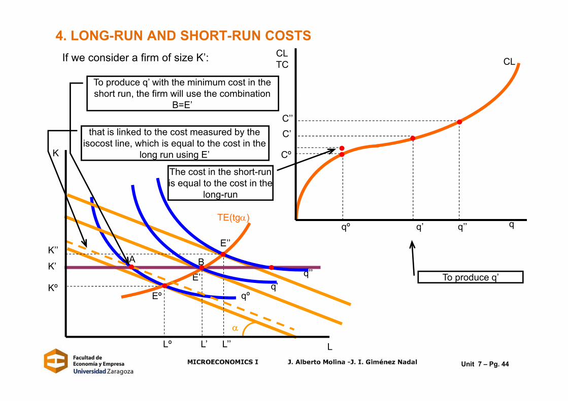
To produce q’

To produce q’ with the minimum cost in the short run, the firm will use the combination

B=E’

that is linked to the cost measured by the isocost line, which is equal to the cost in the

long run using E’

The cost in the short-run is equal to the cost in the

long-run



Unit 7 – Pg. 44

Only for q’ costs in the‐short and long‐run are equal, for any other amount of input the cost in the short‐run is larger than the cost in the short‐run, as there is a size of the firm that better suits, compared to K’

L

K

qº

TE(tg)

Eº

Lº L’

q’q’’E’

E’’

L’’

A B CK’

Kº

K’’

q

CLTC

qº q’ q’’

Cº

C’

C’’

TC(K’) CL

to porduce q’’

To produce q’’ with the minimum cost in the short run, the firm will use the combination C

that is linked to the cost measured by the isocost line, that is higher than the cost in the long-run in E’’

The cost in the short-run is larger than the cost in the

short-run

The cost function in the short-run for a firm of size K’ has been obtained, in relation to the cost function in the long-run

4. LONG-RUN AND SHORT-RUN COSTSIf we consider a firm of size K’:

Unit 7 – Pg. 45

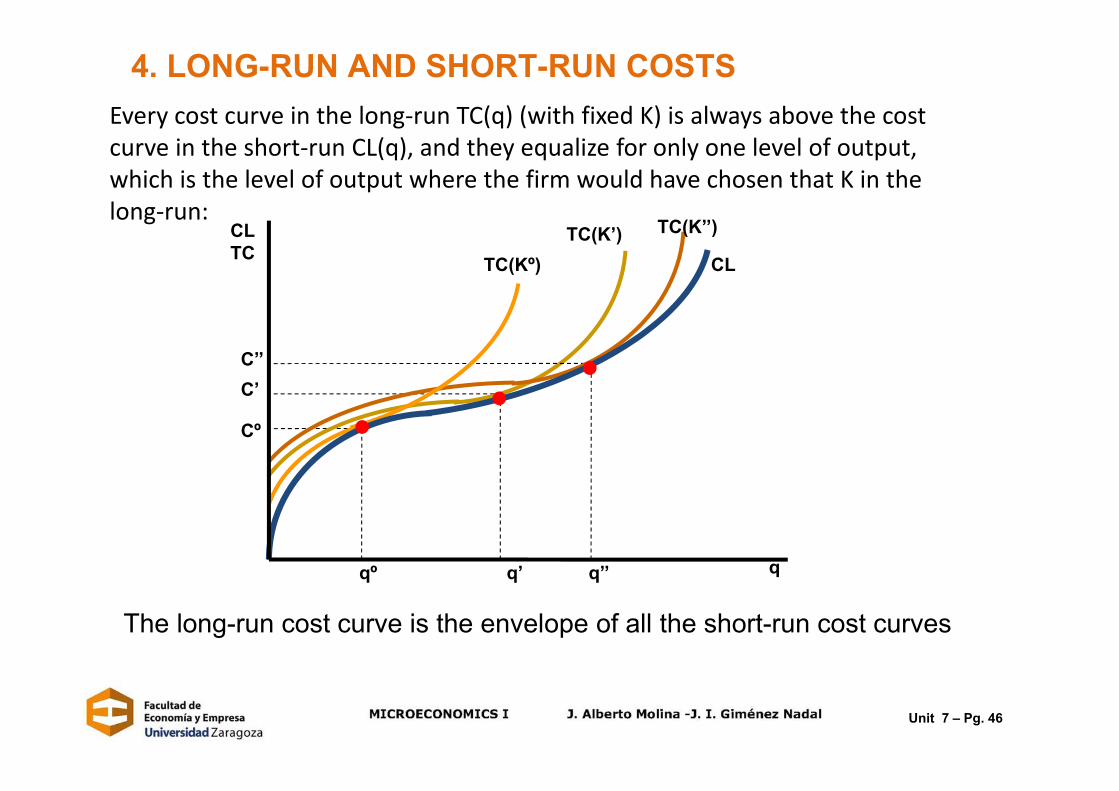
Every cost curve in the long‐run TC(q) (with fixed K) is always above the costcurve in the short‐run CL(q), and they equalize for only one level of output, which is the level of output where the firm would have chosen that K in thelong‐run:

q

CLTC

qº q’ q’’

Cº

C’C’’

TC(K’)CLTC(Kº)

TC(K’’)

The long-run cost curve is the envelope of all the short-run cost curves


Unit 7 – Pg. 46

We have analyzed the problem of cost‐minimization. If we solve it, for a givenamount of output (q), we can determine, given the technology and theprice of the inputs:

• The combination of inputs that minimize the cost• The minimum cost

The next step consists of, assuming that the goal of the firm is to maximizeits profit, in order to answer the following questions:

• How much to produce?• At what prices?That is, what is the amount of production q* that maximizes the profit?The profit function (revenue minus costs):

P(q)=R(q)‐C(q)

5. MARGINAL REVENUE, MARGINAL COST AND PROFIT MAXIMIZATION

Unit 7 – Pg 47

qmax (q) R(q) C(q)

The elements to solve the profit-maximization problem are:

1.The technology

2.The price of the inputs

3.The market demand

4.The type of competition [Micro II]

Independently of the type of competition, the firm always has a Revenue function, which links, to each amount of output q, the income generated by the sale of the output (sell price x produced units):

R=p.q=R(q)


Goal: maximize the profit:

•Optimization problem without restrictions

•There is only one decision variable (q)

Unit 7 – Pg. 48

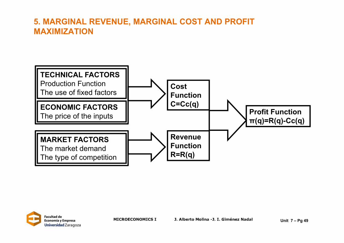
TECHNICAL FACTORSProduction FunctionThe use of fixed factors

ECONOMIC FACTORSThe price of the inputs

MARKET FACTORSThe market demandThe type of competition

Cost FunctionC=Cc(q)

Revenue FunctionR=R(q)

Profit Functionπ(q)=R(q)-Cc(q)


Unit 7 – Pg 49

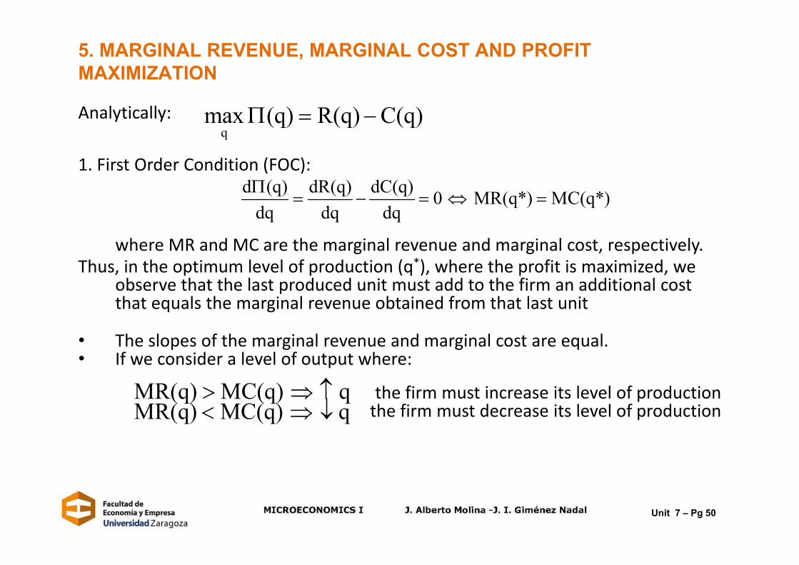
Analytically:

1. First Order Condition (FOC):

where MR and MC are the marginal revenue and marginal cost, respectively.Thus, in the optimum level of production (q*), where the profit is maximized, we

observe that the last produced unit must add to the firm an additional costthat equals the marginal revenue obtained from that last unit

• The slopes of the marginal revenue and marginal cost are equal.• If we consider a level of output where:

the firm must increase its level of productionthe firm must decrease its level of production

d (q) dR(q) dC(q) 0 MR(q*) MC(q*)dq dq dq

MR(q) MC(q) qMR(q) MC(q) q

qmax (q) R(q) C(q)


Unit 7 – Pg 50

q

q

R(q)CL(q)

π(q)

R(q)CL(q)

π(q)

q*

q*


Unit 7 – Pg. 51

2. Second Order Condition (SOC):

• The profit function must be concave

3. Economic condition: the firm will produce only if the profit from producing ishigher than or equal to the profit from no production (shutting down)

2 2 2 * *

2 2 2

d Π(q) d R(q) d C(q) dMR(q ) dMC(q )0 0 0dq dq dq dq dq

If (q*) (q 0) firm must produce q*the

If (q*) (q 0) the firm should shut down


Unit 7 – Pg. 52

Exercises1.- Consider the following production function: where K is capital and Lis labor. The prices of the inputs are r=2 and w=1, respectively:

a)Define the concept of economic efficiency.b)Obtain the Conditional Factor Demands and the cost curve. What is the

minimum cost in the long-run to produce 10 units of output? How manyunits of K and L must the firm use in order to be economically efficient?

c) Represent graphically the cost curve in the long-run, and the Average Costand Marginal Cost curves. Is there any relationship between the returns toscale of the technology and the form of these curves?

d)Determine the elasticity function of the total cost.

2.- Consider the following production function: where K is capital and Lis labor. The prices of the inputs are r=1 and w=2, respectively:

a)Represent graphically the cost curve in the long-run, and the Average Costand Marginal Cost curves.

b)Explain the relationship between the returns to scale and the cost curve inthe long-run of the firm.

Unit 7 – Pg. 53

3.- The production function of a firm is given by . Currently the firm isproducing a level of q=100, but due to a large increase in demand the firm wantsto increase production by 300 units (q=400). The firm has predicted that such anincrease will lead to an increase of the long-run cost of 14,000 m.u. Is thisprediction correct, knowing that the price of the inputs are w=r=1? What is thecombination of inputs that will allow the firm to obtain that increase in the output?

4.- Consider a firm that employs capital K and labor L. The price of the inputs is 1.Define the concept of Conditional Factor Demands. If the Conditional FactorDemands in the long-run of the firm are , explain the type of returns toscale of the production function.

5.- The competitive firm CONSULTING&YOU is in the marketing business. Theproduction cost in the long-run is given by the function(where q indicates the number of monthly reports). Due to a large increase indemand, the firm wants to double its production and has decided to double all itsinputs. Is this correct?

Unit 7 – Pg. 54

6.- Let be the production function of a firm, where K is capital and L is labor. Theprices of the inputs are r=2 and w=2:

a) Assume that in the short-run the input K is fixed at K=2. Obtain the cost curve in theshort-run. Does the Law of Diminishing Returns applied?

b) Obtain the Marginal Cost, Average Variable Cost, and Average Total Cost curves.c) What is the maximum level of output that in the short-run could be produced with

204 m.u.?d) Assume that the firm wants to produce 50 units of output. What is the minimum cost

that allows the firm to produce that level in the short-run? How many units of K andL should the firm employ?

7.- Let be the production function of a firm. The price of K is r=4 and of L is w=1.a) Assume that in the short-run the input K is fixed at K=2. Obtain the cost curve in the

short-run, and the Marginal Cost, Average Variable Cost, and Average Total Costcurves.

b) Obtain the cost curve in the long-run, and the Average Cost and Marginal Costcurves.

c) Will the firm have a higher cost in the long-run or in the short-run if it wants toproduce q=100?

d) What is the maximum level of output that in the long-run can be produced with 3,000m.u.? What combination of factors should the firm employ?

Unit 7 – Pg. 55

8.- Obtain the Fixed Cost (FC) of a firm that in the Optimum EfficientScale (qOES) produces q=5, knowing that the Marginal Cost is:MC = 9q2 - 30q + 50

9.- Given that the Marginal Cost function for a firm is MC = 3 + 8q +15q2,obtain the corresponding total cost curve if it is known that in q=4, thetotal cost of production is 896 m.u.

10.- A firm has a production technology represented by the function:

The prices of the inputs are: w=10 and r=2. Determine the minimum costthe firm will have to produce 160,000 units of output.

Unit 7 – Pg. 56

11.- A firm has a production technology represented by the function .The prices of the inputs are w=5 and r=20.

a)Determine the minimum cost that allows the firm to produce 3,400 units ofoutput. Represent it graphically.

b)Obtain the Expansion Path. Represent it graphically.c) Obtain the Conditional Factor Demands functions.d)Obtain the cost functions. Represent them graphically.e)Answer the previous questions if now w=48 and r=3.

12.- A firm has a production technology represented by the function . Theprices of the inputs are w=32 and r=2.

a) Determine the minimum cost that allows the firm to produce 20 units ofoutput.

b) Obtain the maximum level of output that in the long-run can be producedwith 6,400 m.u.

c) Answer the previous questions if now w=8 and r=2.

Unit 7 – Pg. 57

13.- Explain whether the following statements are true or false:a) A firm can be economically efficient and technically inefficient.b) A firm can be economically inefficient and technically efficient.c) If the prices of the inputs a firm employs are equal, cost-minimization will lead the firm to

use equal amounts of inputs.d) The cost-minimization condition is characterized by the fact that the last monetary unit

spent in each input increases the output by the same proportion.e) The Conditional Factor Demands functions indicate, given the price of the inputs, the units

of inputs K and L that minimize the production cost of the firm, for each level of output.f) Any change in the price of one of the inputs will affect the production technology and the

cost curve.g) For any level of output lower than the output associated with the Minimum Average Total

Cost (qMATC), the Marginal Cost is higher than the Average Variable Cost.h) Since the Fixed Cost (FC) does not depend on the level of output, the average fixed cost

is constant.i) With constant returns to scale, the Average Cost function is perfectly elastic.j) According to the “Law of Equality of the Weighted Marginal Productivity (LEWMP)” a firm

minimizes its cost when the expenditure on each of the inputs is equal (the firm spendsthe same monetary units on each factor).

k) The level of output associated with the Minimum Average Variable Cost (qMAVC)represents the output from where the Marginal Cost is higher than the Average VariableCost.

l) The area under the Marginal Cost function in the short-run measures the variable cost.m) The area under the Marginal Cost function in the long-run measures the total cost.

Unit 7 – Pg. 58

14.- Explain whether the following statements are true or false. With increasingreturns to scale:

a) If all the inputs, except one, increase by a given proportion, the outputincreases by a higher proportion.

b) If the employment level of all the inputs is reduced by 50%, the outputalso decreases, but by a proportion less than 50%.

c) The Law of Diminishing Returns can never be satisfied.

15.- A competitive firm produces a good “Q” employing two variable inputs, X1 andX2 whose prices are r1=2, r2=6. As a consultant, the producer tells you: “currently,I am producing 100 units of output, employing 10 units of X1 and 20 of X2. Withthe last employed unit of X1 the production increased by 4 units, while with thelast employed unit of X2 the production increased by 8 units.” With thisinformation, what would you recommend the producer do regarding thecombination of employed inputs?

Unit 7 – Pg. 59

16.- Given a firm whose Marginal Product for inputs X1 and X2 are f1=8, f2=4 ,and the prices of the inputs are r1=4, r2=2. Explain the statement(s) you thinkis(are) true:

a) It cannot produce more output at the same cost.b) It must increase X2 and decrease X1 in order to minimize costs.c) It must decrease X2 and increase X1 in order to minimize costs.d) It cannot produce the same level of output at a lower cost.

17.- A firm is able to produce 20 units of a good Q at minimum cost, employingthe inputs K and L, whose prices are r=3 and w=2, respectively. The firm arguesthat the increase in the production associated with the last monetary unit spent ininput L is equal to 6:

a) Calculate the Marginal Product of the last monetary unit spent in input L.b) Calculate the increase in the output associated with the last employed

unit of L.

Unit 7 – Pg. 60

18.- A firm is producing 18,000 units of output per month, employing acombination of inputs that has a Marginal Rate of Technical Substitution(MRTS) lower than the ratio of the input prices. How is the firm able toreduce its costs?

19.- The combination of inputs that allows the firm to minimize theproduction cost is the one where:

a)the isoquant curve and the isocost line are tangent.b)the value of the MRTS is equal to the ratio of prices.c)the last monetary unit spent in each input increases the outputequally.d)the last unit employed of each input increases the output equally.

20.- Explain the “Law of Equality of the Weighted Marginal Productivity(LEWMP)”

Unit 7 – Pg. 61

21.- If the prices of the inputs employed by a firm are equal, cost-minimization will lead the firm to:

a) employ the same units of all inputs.b) increase the level of input L so that the last monetary unit spent on

it produces a greater increase in the level of output.c) employ a combination of inputs that makes equal the Marginal

Product.d) increase the level of the input with the lowest Marginal Product.e) increase the level of the input with the highest Marginal Product.

22.- Explain which of the previous statements are true when the prices ofthe inputs are not equal.

Unit 7 – Pg. 62

23.- Consider a firm that has a production function q=f(L,K) presenting constantreturns to scale. It is known that to produce 10 units of output the firm employs 6units of K and 4 of L.

a) If the prices of the inputs are r=2 and w=2, respectively, how many unitsof K and L will the firm employ when its total cost is 100 m.u., and howmuch will it produce?

b) Assume that the technology presents decreasing returns to scale. Will thefirm be able to produce 15 units of output with a cost of 30 m.u.? And witha cost of 40 m.u?

24.- a) Explain the conditions that determine the level of production thatmaximizes the revenue of a firm in the short-run and the long-run, for any type ofmarket structure.

b) Consider a firm that in the short-run is producing a level of output sothat MR>MC, and obtains a profit of 30,000 monetary units. Is the firm maximizingits profit? Why? Would you recommend the firm increase or decrease its level ofproduction?

Unit 7 – Pg. 63

25.- Assume that you must advise a firm about the volume of output thatmaximizes the firm’s profit in the short-run. The firm gives you thefollowing information:

Level of Output………….. 100 unitsMarginal Revenue…………10 €urosMarginal Cost……………...10 €urosTotal Revenue……………..1000 €urosTotal Cost…………………..1200 €urosFixed Cost…………………..300 €urosWhat should you advise the firm?

1) Increase the level of output.2) Decrease the level of output (to a level q>0).3) Stop producing.4) Do not change the level of output.

Unit 7 – Pg. 64

26.- Assume the production function q=f(L,K) is known, and also the prices of theinputs: w0 and r0. Show graphically how the Expansion Path and the cost functionin the long-run are affected if:

a) W increases.b) R increases.

27.- Assume the production function q=f(L,K) is known, and also the prices of theinputs: w0 and r0. Determine how the Conditional Factor Demand of the variableinput in the short-run is affected, and show graphically how the cost functions inthe short-run are affected for a firm of size K=K0:

a) W increases.b) R increases.

28.- Assume the production function q=f(L,K) is known, and also the prices of theinputs: w0 and r0. Determine and show graphically how the Expansion Path, theConditional Factor Demand, and the cost functions in the long-run are affected byan increase in the price of the inputs in the same proportion.

Unit 7 – Pg. 65

unit 7: minimizing costs and maximizing …personal.unizar.es/jamolina/_/microeconomia/unit...

Documents