uniform flow and flow resistance copyright © 2009. oxford...
TRANSCRIPT

6
Uniform Flow and FlowResistance
6.0 Introduction and Overview
The central problem of open-channel-flow hydraulics can be stated as follows: Givena channel reach with a specified geometry, material, and slope, what are the relationsamong flow depth, average velocity, width, and discharge? Solutions to this problemare essential for solving important practical problems, including 1) the design ofchannels and canals, 2) the areal extent of flooding that will result from a storm orsnowmelt event, 3) the rate of travel of a flood wave through a channel network, and4) the size and quantity of material that can be eroded or transported by various flows.
The characterization of flow resistance (defined precisely in section 6.4) is essentialto the solutions of this central problem, because it provides the relation betweenvelocity (usually considered the dependent variable) and 1) specified geometricand boundary characteristics of the channel, usually considered to be essentiallyconstant; and 2) the flow magnitude expressed as discharge or depth, considered asthe independent variable that may change with time in a given reach.
The definition of flow resistance is developed from the concepts of uniform flow(section 4.2.1.2) and force balance (section 4.7). Recall that in a steady uniform flow,there is no acceleration; thus, by Newton’s second law of motion, there is no net forceacting on the fluid. Although uniform flow is an ideal state seldom strictly achievedin natural flows, it is often a valid assumption because open-channel flows are self-adjusting dynamic systems (negative feedback loops) that are always tending towarda balance of driving and resisting forces: an increase (decrease) in velocity producesan increase (decrease) in resistance tending to decrease (increase) velocity.
211
Copyright © 2009. Oxford University Press. All rights reserved. May not be reproduced in any form without permission from the publisher, except fair uses permitted under
U.S. or applicable copyright law.
EBSCO Publishing : eBook Academic Collection (EBSCOhost) - printed on 2/19/2017 4:55 PM viaUNIV OF CHICAGOAN: 271150 ; Dingman, S. L..; Fluvial HydraulicsAccount: s8989984

212 FLUVIAL HYDRAULICS
To better appreciate the basic concepts underlying the definition and determinationof resistance, this chapter begins by reviewing the basic geometric features of riverreaches and reach boundaries presented in section 2.3. We then adapt the definition ofuniform flow as applied to a fluid element to apply to a typical river reach and derivethe Chézy equation, which is the basic equation for macroscopic uniform flows. Thisderivation allows us to formulate a simple definition of resistance. We then undertakean examination of the factors that determine flow resistance; this examination involvesapplying the principles of dimensional analysis developed in section 4.8.2 and thevelocity-profile relations derived in chapter 5. The chapter concludes by exploringresistance in nonuniform flows and practical approaches to determining resistance innatural channels.
As we will see, there is still much research to be done to advance our understandingof resistance in natural rivers.
6.1 Boundary Characteristics
As noted above, the nature as well as the shape of the channel boundary affectsflow resistance. The classification of boundary characteristics in figure 2.15 providesperspective for the discussion in the remainder of this chapter: Most of the analyticalrelations that have been developed and experimental results that have been obtainedare for rigid, impervious, nonalluvial or plane-bed alluvial boundaries, while many,if not most, natural channels fall into other categories.
In this chapter, we consider cross-section-averaged or reach-averaged conditionsrather than local “vertically” averaged velocities (Uw) and local depths (Yw), andwill designate these larger scale averages as U and Y , respectively. Figure 6.1shows the spatial scales typically associated with these terms. Since our analyticalreasoning will be based on the assumption of prismatic channels, there is no distinctionbetween cross-section averaging and reach averaging. We will often invoke the wide
Reach (U, Y )
Cross section (U, Y )
Local (Uw, Yw)
10−3 10−2 10−1 100 101 102 103 104 105
Spatial scale (m)
Figure 6.1 Spatial scales typically associated with local, cross-section-averaged, and reach-averaged velocities, depths, and resistance. After Yen (2002).
Copyright © 2009. Oxford University Press. All rights reserved. May not be reproduced in any form without permission from the publisher, except fair uses permitted under
U.S. or applicable copyright law.
EBSCO Publishing : eBook Academic Collection (EBSCOhost) - printed on 2/19/2017 4:55 PM viaUNIV OF CHICAGOAN: 271150 ; Dingman, S. L..; Fluvial HydraulicsAccount: s8989984

UNIFORM FLOW AND FLOW RESISTANCE 213
open-channel concept to justify applying the local, two-dimensional “vertical”velocity distributions discussed in chapter 5 [especially the Prandtl-von Kármán(P-vK) law] to entire cross sections.
We saw in section 5.3.1.6 that channel boundaries can be hydraulically “smooth”or “rough” depending on whether the boundary Reynolds number Reb is greater orless than 5, where
Reb ≡ u∗·yr
�(6.1)
u∗ is shear velocity, � is kinematic viscosity, and yr is the roughness height, that is,the characteristic height of roughness elements (projections) on the boundary (seefigure 5.7). In natural alluvial channels, the bed material usually consists of sedimentgrains with a range of diameters (figure 2.17a). For a particular reach the characteristicheight yr is usually determined as shown in figure 2.17b:
yr = kr ·dp, (6.2)
where dp is the diameter of particles larger than p percent of the particles on theboundary surface and kr is a multiplier ≥1. Different investigators have used differentvalues for p and kr (see Chang 1988, p. 50); we will generally assume kr = 1 andp = 84 so that yr = d84.
Of course, other aspects of the boundary affect the effective roughness height,especially the spacing and shape of particles. And, as suggested in figure 2.15, theappropriate value for yr is affected by the presence of bedforms, growing and deadvegetation, and other factors.
6.2 Uniform Flow in Open Channels
6.2.1 Basic Definition
The concepts of steady flow and uniform flow were introduced in section 4.2.1.2 inthe context of the movement of a fluid element in the x-direction along a streamline:
If the element velocity u at a given point on a streamline does not change withtime, the flow is steady (local acceleration du/dt = 0); otherwise, it isunsteady.If the element velocity at any instant is constant along a streamline, the flow isuniform (convective acceleration du/dx = 0); otherwise, it is nonuniform.
In the remainder of this text we will be concerned with the entirety of a flowwithin a reach of finite length rather than an individual fluid element flowing alonga streamline. Furthermore, in turbulent flows, which include the great majority ofnatural open-channel flows, turbulent eddies preclude the existence of strictly steadyor uniform flow. To account for these conditions we must modify the definition of“steady” and “uniform.” To do this, we first designate the X-coordinate direction as thedownstream direction for a reach and define U as the downstream-directed velocity,
Copyright © 2009. Oxford University Press. All rights reserved. May not be reproduced in any form without permission from the publisher, except fair uses permitted under
U.S. or applicable copyright law.
EBSCO Publishing : eBook Academic Collection (EBSCOhost) - printed on 2/19/2017 4:55 PM viaUNIV OF CHICAGOAN: 271150 ; Dingman, S. L..; Fluvial HydraulicsAccount: s8989984

214 FLUVIAL HYDRAULICS
1) time-averaged over a period longer than the time scale of turbulent fluctuationsand 2) space-averaged over a cross section. Then,
• In steady flow, dU/dt = 0 at any cross section.• In uniform flow, dU/dX = 0 at any instant.
As noted by Chow (1959, p. 89), unsteady uniform flow is virtually impossible ofoccurrence. Thus, henceforth, “uniform flow” implies “steady uniform flow.” Note,however, that a nonuniform flow may be steady or unsteady.
We will usually assume that the discharge, Q, in a reach is constant in space andtime, where
Q = W ·Y ·U, (6.3)
W is the water-surface width, and Y is average depth.In uniform flow with spatially constant Q, it must also be true that depth and width
are constant, so “uniform flow” implies dY /dX = 0 and dW /dX = 0.1 And, sincethe depth does not change, “uniform flow” implies that the water-surface slope isidentical to the channel slope. Thus, it must also be true that for strictly uniform flow,cross-section shape is constant through a reach (i.e., the channel is prismatic).
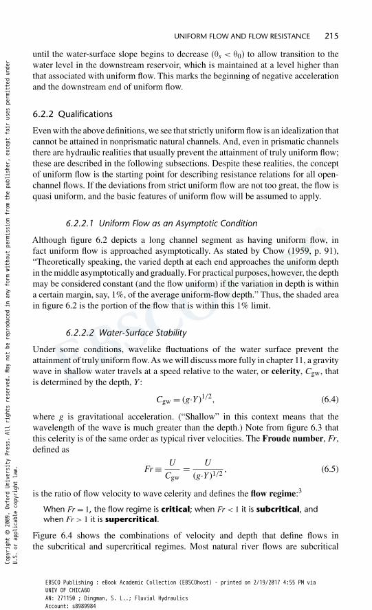
Figure 6.2 further illustrates the concept of uniform flow. Here, a river or canal withconstant channel slope �0, geometry, and bed and bank material, and no other inputsof water, connects two large reservoirs that maintain constant surface elevations.Under these conditions, the discharge will be constant along the entire channel.As the water leaves the upstream reservoir, it accelerates from zero velocity dueto the downslope component of gravity, g·sin�s, where �s is the local slope of thewater surface. As it accelerates, the frictional resistance of the boundary is transmittedinto the fluid by viscosity and turbulence (as in figure 3.28). This resistance increasesas the velocity increases and soon balances the gravitational force,2 at which pointthere is no further acceleration. Downstream of this point, the water-surface slope �s
equals the channel slope �0, the cross-section-averaged velocity and depth becomeconstant, and uniform flow is established. The velocity and depth remain constant
θS
θ0
Figure 6.2 Idealized development of uniform flow in a channel of constant slope, �0, geometry,and bed material connecting two reservoirs. The shaded area is the region of uniform flow, wherethe downstream component of gravity is balanced by frictional resistance and the water-surfaceslope �S equals �0.
Copyright © 2009. Oxford University Press. All rights reserved. May not be reproduced in any form without permission from the publisher, except fair uses permitted under
U.S. or applicable copyright law.
EBSCO Publishing : eBook Academic Collection (EBSCOhost) - printed on 2/19/2017 4:55 PM viaUNIV OF CHICAGOAN: 271150 ; Dingman, S. L..; Fluvial HydraulicsAccount: s8989984
UNIFORM FLOW AND FLOW RESISTANCE 215
until the water-surface slope begins to decrease (�s < �0) to allow transition to thewater level in the downstream reservoir, which is maintained at a level higher thanthat associated with uniform flow. This marks the beginning of negative accelerationand the downstream end of uniform flow.
6.2.2 Qualifications
Even with the above definitions, we see that strictly uniform flow is an idealization thatcannot be attained in nonprismatic natural channels. And, even in prismatic channelsthere are hydraulic realities that usually prevent the attainment of truly uniform flow;these are described in the following subsections. Despite these realities, the conceptof uniform flow is the starting point for describing resistance relations for all open-channel flows. If the deviations from strict uniform flow are not too great, the flow isquasi uniform, and the basic features of uniform flow will be assumed to apply.
6.2.2.1 Uniform Flow as an Asymptotic Condition
Although figure 6.2 depicts a long channel segment as having uniform flow, infact uniform flow is approached asymptotically. As stated by Chow (1959, p. 91),“Theoretically speaking, the varied depth at each end approaches the uniform depthin the middle asymptotically and gradually. For practical purposes, however, the depthmay be considered constant (and the flow uniform) if the variation in depth is withina certain margin, say, 1%, of the average uniform-flow depth.” Thus, the shaded areain figure 6.2 is the portion of the flow that is within this 1% limit.
6.2.2.2 Water-Surface Stability
Under some conditions, wavelike fluctuations of the water surface prevent theattainment of truly uniform flow.As we will discuss more fully in chapter 11, a gravitywave in shallow water travels at a speed relative to the water, or celerity, Cgw, thatis determined by the depth, Y :
Cgw = (g·Y )1/2, (6.4)
where g is gravitational acceleration. (“Shallow” in this context means that thewavelength of the wave is much greater than the depth.) Note from figure 6.3 thatthis celerity is of the same order as typical river velocities. The Froude number, Fr,defined as
Fr ≡ U
Cgw= U
(g·Y )1/2, (6.5)
is the ratio of flow velocity to wave celerity and defines the flow regime:3
When Fr = 1, the flow regime is critical; when Fr < 1 it is subcritical, andwhen Fr > 1 it is supercritical.
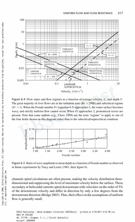
Figure 6.4 shows the combinations of velocity and depth that define flows inthe subcritical and supercritical regimes. Most natural river flows are subcritical
Copyright © 2009. Oxford University Press. All rights reserved. May not be reproduced in any form without permission from the publisher, except fair uses permitted under
U.S. or applicable copyright law.
EBSCO Publishing : eBook Academic Collection (EBSCOhost) - printed on 2/19/2017 4:55 PM viaUNIV OF CHICAGOAN: 271150 ; Dingman, S. L..; Fluvial HydraulicsAccount: s8989984

216 FLUVIAL HYDRAULICS
1
10
100
1001010.1Depth, Y (m)
Cel
erity
,Cg
w (
m/s
)
Figure 6.3 Celerity of shallow-water gravity waves, Cgw, as a function of flow depth, Y(equation 6.4). Note that Cgw is of the same order of magnitude as typical river velocities.
(Grant 1997), but when the slope is very steep and/or the channel material isvery smooth (as in some bedrock channels and streams on glaciers, and at localsteepenings in mountain streams), the Froude number may approach or exceed 1.When Fr approaches 1, waves begin to appear in the free surface, and strictlyuniform flow is not possible. In channels with rigid boundaries, the amplitudeof these waves increases approximately linearly with Fr (figure 6.5). When Frapproaches 2 (Koloseus and Davidian 1966), the flow will spontaneously formroll waves—the waves you often see on a steep roadway or driveway duringa rainstorm (figure 6.6). However, this situation is unusual in natural channels.In channels with erodible boundaries (sand and gravel), wavelike bedforms calleddunes or antidunes begin to form when Fr approaches 1. The water surfacealso becomes wavy, either out of phase (dunes) or in phase (antidunes) with thebedforms; these are discussed further in section 6.6.4 and in sections 10.2.1.5and 12.5.4.
In situations where surface instabilities occur, it may be acceptable to relax thedefinition of “uniform” by averaging dU/dX and dY /dX over distances greater thanthe wavelength of the surface waves.
6.2.2.3 Secondary Currents
The concept of uniform flow as described in section 6.2.1 implicitly assumes thatflow is the downstream direction only, and this assumption underlies most of theanalyses in this text. However, as we saw in section 5.4.2, even in straight rectangular
Copyright © 2009. Oxford University Press. All rights reserved. May not be reproduced in any form without permission from the publisher, except fair uses permitted under
U.S. or applicable copyright law.
EBSCO Publishing : eBook Academic Collection (EBSCOhost) - printed on 2/19/2017 4:55 PM viaUNIV OF CHICAGOAN: 271150 ; Dingman, S. L..; Fluvial HydraulicsAccount: s8989984
UNIFORM FLOW AND FLOW RESISTANCE 217
0.001
0.01
0.01 0.1 1 10
0.1
1
10
100
Velocity, U (m s–1)
TURBULENTSUBCRITICAL
TURBULENTSUPERCRITICAL
LAMINARSUBCRITICAL
TRANSITIONALSUBCRITICAL
TRANSITIONALSUPERCRITICAL
LAMINARSUPERCRITICAL
Fr = 1
Fr = 2 Re = 2000
Re = 500
Dep
th,Y
(m
)
Figure 6.4 Flow states and flow regimes as a function of average velocity, U, and depth Y .The great majority of river flows are in the turbulent state (Re > 2000) and subcritical regime(Fr < 1). When the Froude number Fr (equation 6.5) approaches 1, the water surface becomeswavy, and strictly uniform flow cannot occur. When Fr approaches 2, pronounced waves arepresent. Note that some authors (e.g., Chow 1959) use the term “regime” to apply to one ofthe four fields shown on this diagram rather than to the subcritical/supercritical condition.
Am
plit
ude/
Dep
th 0.10
0.05
0
Froude number
1.00 1.50 2.00 2.50 3.00 3.50 4.00
Figure 6.5 Ratio of wave amplitude to mean depth as a function of Froude number as observedin flume experiments by Tracy and Lester (1961, their figure 6).
channels spiral circulations are often present, making the velocity distribution three-dimensional and suppressing the level of maximum velocity below the surface. Thesesecondary or helicoidal currents spiral downstream with velocities on the order of 5%of the downstream velocity and differ in direction by only a few degrees from thedownstream direction (Bridge 2003). Thus, their effect on the assumptions of uniformflow is generally small.
Copyright © 2009. Oxford University Press. All rights reserved. May not be reproduced in any form without permission from the publisher, except fair uses permitted under
U.S. or applicable copyright law.
EBSCO Publishing : eBook Academic Collection (EBSCOhost) - printed on 2/19/2017 4:55 PM viaUNIV OF CHICAGOAN: 271150 ; Dingman, S. L..; Fluvial HydraulicsAccount: s8989984

218 FLUVIAL HYDRAULICS
Roll waves
Figure 6.6 Roll waves on a steep driveway during a rainstorm. These waves form when theFroude number approaches 2. Photo by the author.
6.3 Basic Equation of Uniform Flow: The Chézy Equation
In this section, we derive the basic equation for strictly uniform flow. Thisequation forms the basis for understanding fundamental resistance relations and otherimportant aspects of flows in channel reaches.
Because there is no acceleration in a uniform flow, Newton’s second law statesthat there are no net forces acting on the fluid and that
FD = FR, (6.6)
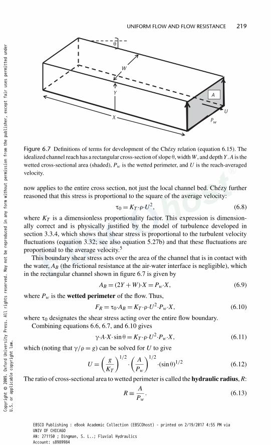
where FD represents the net forces tending to cause motion, and FR represents thenet forces tending to resist motion. The French engineer Antoine Chézy (1718–1798)was the first to develop a relation between flow velocity and channel characteristicsfrom the fundamental force relation of equation 6.6.4 Referring to the idealizedrectangular channel reach of figure 6.7, Chézy expressed the downslope componentof the gravitational force acting on the water in a channel reach, FD, as
FD = �·W ·Y ·X·sin� = �·A·X·sin�, (6.7)
where � is the weight density of water, A is the cross-sectional area of the flow,and � denotes the slope of the water surface and the channel, which are equal inuniform flow.
Chézy noted that the resistance forces are due to a boundary shear stress �0 [F L−2]caused by boundary friction. This is the same quantity defined in equation 5.7, but
Copyright © 2009. Oxford University Press. All rights reserved. May not be reproduced in any form without permission from the publisher, except fair uses permitted under
U.S. or applicable copyright law.
EBSCO Publishing : eBook Academic Collection (EBSCOhost) - printed on 2/19/2017 4:55 PM viaUNIV OF CHICAGOAN: 271150 ; Dingman, S. L..; Fluvial HydraulicsAccount: s8989984
UNIFORM FLOW AND FLOW RESISTANCE 219
θ
W
Y
U X Pw
A
Figure 6.7 Definitions of terms for development of the Chézy relation (equation 6.15). Theidealized channel reach has a rectangular cross-section of slope �, width W , and depth Y . A is thewetted cross-sectional area (shaded), Pw is the wetted perimeter, and U is the reach-averagedvelocity.
now applies to the entire cross section, not just the local channel bed. Chézy furtherreasoned that this stress is proportional to the square of the average velocity:
�0 = KT ·�·U2, (6.8)
where KT is a dimensionless proportionality factor. This expression is dimension-ally correct and is physically justified by the model of turbulence developed insection 3.3.4, which shows that shear stress is proportional to the turbulent velocityfluctuations (equation 3.32; see also equation 5.27b) and that these fluctuations areproportional to the average velocity.5
This boundary shear stress acts over the area of the channel that is in contact withthe water, AB (the frictional resistance at the air-water interface is negligible), whichin the rectangular channel shown in figure 6.7 is given by
AB = (2Y + W )·X = Pw·X, (6.9)
where Pw is the wetted perimeter of the flow. Thus,
FR = �0·AB = KT ·�·U2·Pw·X, (6.10)
where �0 designates the shear stress acting over the entire flow boundary.Combining equations 6.6, 6.7, and 6.10 gives
�·A·X·sin� = KT ·�·U2·Pw·X, (6.11)
which (noting that �/� = g) can be solved for U to give
U =(
g
KT
)1/2
·(
A
Pw
)1/2
·(sin�)1/2 (6.12)
The ratio of cross-sectional area to wetted perimeter is called the hydraulic radius, R:
R ≡ A
Pw. (6.13)
Copyright © 2009. Oxford University Press. All rights reserved. May not be reproduced in any form without permission from the publisher, except fair uses permitted under
U.S. or applicable copyright law.
EBSCO Publishing : eBook Academic Collection (EBSCOhost) - printed on 2/19/2017 4:55 PM viaUNIV OF CHICAGOAN: 271150 ; Dingman, S. L..; Fluvial HydraulicsAccount: s8989984

220 FLUVIAL HYDRAULICS
Incorporating equation 6.13 and defining
S ≡ sin�, (6.14)
We can write the Chézy equation as
U =(
1
KT
)1/2
·(g·R·S)1/2. (6.15a)
For “wide” channels we can approximate the hydraulic radius by the average depth.Thus, we can usually write the Chézy equation as
U =(
1
KT
)1/2
·(g·Y ·S)1/2. (6.15b)
In engineering contexts, the Chézy equation is usually written as described in box 6.1.The Chézy equation is the basic uniform-flow equation and is the basis for
describing the relations among the cross-section or reach-averaged values of thefundamental hydraulic variables velocity, depth, slope, and channel characteristics.It provides a partial answer to the central question posed at the beginning of thechapter, as we have found that
The average velocity of a uniform open-channel flow is proportional to thesquare root of the product of hydraulic radius (R) and the downslopecomponent of gravitational acceleration (g·S).
Also note that the Chézy equation was developed from force-balance considerationsand is a macroscopic version of the general conductance relation (equation 4.54,section 4.7). The Chézy equation was derived by considering the water in the channelas a “block” interacting with the channel boundary; we did not consider phenomenawithin the “block” except to justify the relation between �0 and the square of thevelocity (equation 6.8).
A more complete answer to the central question posed at the beginning of thischapter requires some way of determining the value of KT . This quantity is theproportionality between the shear stress due to the boundary and the square of thevelocity; thus, presumably it depends in some way on the nature of the boundary.Most of the rest of this chapter explores the relation between this proportionality andthe nature of the boundary. We will see that the velocity profiles derived in chapter 5along with experimental observations provide much of the basis for formulating thisrelation. But before proceeding to that exploration, we use the Chézy derivation toformulate the working definition of resistance.
6.4 Definition of Reach Resistance
By comparison with equation 5.24, the quantity (g·R·S)1/2 can be considered to bethe reach-averaged shear velocity, so henceforth
u∗ ≡ (g·R·S)1/2. (6.16a)
Again, we have seen that we can usually approximate this definition as
u∗ = (g·Y ·S0)1/2. (6.16b)
Copyright © 2009. Oxford University Press. All rights reserved. May not be reproduced in any form without permission from the publisher, except fair uses permitted under
U.S. or applicable copyright law.
EBSCO Publishing : eBook Academic Collection (EBSCOhost) - printed on 2/19/2017 4:55 PM viaUNIV OF CHICAGOAN: 271150 ; Dingman, S. L..; Fluvial HydraulicsAccount: s8989984
UNIFORM FLOW AND FLOW RESISTANCE 221
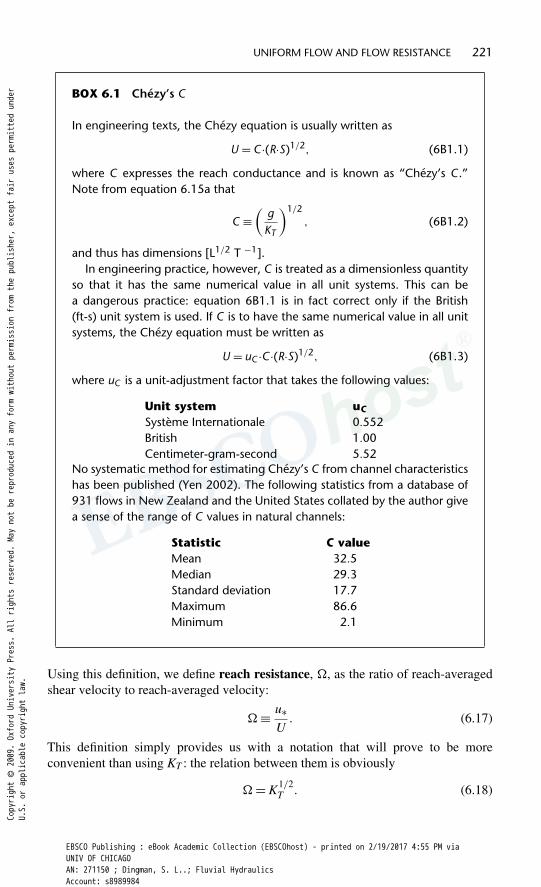
BOX 6.1 Chézy’s C
In engineering texts, the Chézy equation is usually written as
U = C ·(R·S)1/2, (6B1.1)
where C expresses the reach conductance and is known as “Chézy’s C .”Note from equation 6.15a that
C ≡(
gKT
)1/2, (6B1.2)
and thus has dimensions [L1/2 T −1].In engineering practice, however, C is treated as a dimensionless quantity
so that it has the same numerical value in all unit systems. This can bea dangerous practice: equation 6B1.1 is in fact correct only if the British(ft-s) unit system is used. If C is to have the same numerical value in all unitsystems, the Chézy equation must be written as
U = uC ·C ·(R·S)1/2, (6B1.3)
where uC is a unit-adjustment factor that takes the following values:
Unit system uCSystème Internationale 0.552British 1.00Centimeter-gram-second 5.52
No systematic method for estimating Chézy’s C from channel characteristicshas been published (Yen 2002). The following statistics from a database of931 flows in New Zealand and the United States collated by the author givea sense of the range of C values in natural channels:
Statistic C valueMean 32.5Median 29.3Standard deviation 17.7Maximum 86.6Minimum 2.1
Using this definition, we define reach resistance, �, as the ratio of reach-averagedshear velocity to reach-averaged velocity:
� ≡ u∗U
. (6.17)
This definition simply provides us with a notation that will prove to be moreconvenient than using KT : the relation between them is obviously
� = K1/2T . (6.18)
Copyright © 2009. Oxford University Press. All rights reserved. May not be reproduced in any form without permission from the publisher, except fair uses permitted under
U.S. or applicable copyright law.
EBSCO Publishing : eBook Academic Collection (EBSCOhost) - printed on 2/19/2017 4:55 PM viaUNIV OF CHICAGOAN: 271150 ; Dingman, S. L..; Fluvial HydraulicsAccount: s8989984
222 FLUVIAL HYDRAULICS
Box 6.2 defines the Darcy-Weisbach friction factor, a dimensionless resistancefactor that is commonly used as an alternative to KT and �.
Note that using equation 6.17, we can rewrite the Chézy equation as
U = �−1·u∗. (6.19)
BOX 6.2 The Darcy-Weisbach Friction Factor
In 1845 Julius Weisbach (1806–1871) published the results of pioneeringexperiments to determine frictional resistance in pipe flow (Rouse andInce 1963) and formulated a dimensionless factor, fDW, that expresses thisresistance:
fDW ≡ 2·(
he
X
)·(
D·gU2
), (6B2.1)
where he (L) is the loss in mechanical energy per unit weight of water, or head(see equation 4.45) in distance X, D is the pipe diameter, U is the average flowvelocity, and g is gravitational acceleration. In 1857, the same Henry Darcy(1803–1858) whose experiments led to Darcy’s law, the central formula ofgroundwater hydraulics, published the results of similar pipe experiments,and fDW is known as the Darcy-Weisbach friction factor.
The pipe diameter D equals four times the hydraulic radius, R, so
fDW ≡ 8·(
he
X
)·(
R·gU2
). (6B2.2)
The quantity he/X in pipe flow is physically identical to the channel andwater-surface slope, S ≡ sin �, in uniform open-channel flow, so the frictionfactor for open-channel flow is
fDW ≡ 8·g·R·SU2 . (6B2.3a)
From the definition of shear velocity, u∗ (equation 6.16a), 6B2.3a can alsobe written as
fDW = 8· u2∗U2 , (6B2.3b)
and from the definition of � (equation 6.17), we see that
fDW = 8·�2; (6B2.4a)
� =(
fDW
8
)1/2= 0.354·fDW
1/2. (6B2.4b)
The Darcy-Weisbach friction factor is commonly used to express resistancein open channels as well as pipes. However, the � notation is used hereinbecause it is simpler: It does not include the 8 multiplier and is written interms of u∗ and U rather than the squares of those quantities.
Copyright © 2009. Oxford University Press. All rights reserved. May not be reproduced in any form without permission from the publisher, except fair uses permitted under
U.S. or applicable copyright law.
EBSCO Publishing : eBook Academic Collection (EBSCOhost) - printed on 2/19/2017 4:55 PM viaUNIV OF CHICAGOAN: 271150 ; Dingman, S. L..; Fluvial HydraulicsAccount: s8989984
UNIFORM FLOW AND FLOW RESISTANCE 223
The inverse of a resistance is a conductance, so we can define �−1 as thereach conductance, and we can use the two concepts interchangeably. The centralproblem of open-channel flow can now be stated as, “What factors determine thevalue of �?”
6.5 Factors Affecting Reach Resistance in Uniform Flow
In section 4.8.2.2, we used dimensional analysis to derive equation 4.63:
U = f�
(Y
yr,
Y
W,Re
)·(g·Y ·S)1/2 = f�
(Y
yr,
Y
W,Re
)·u∗, (6.20)
where Re is the flow Reynolds number. Thus, we see that the Chézy equation isidentical in form to the open-channel flow relation developed from dimensionalanalysis.And, comparing 6.19 and 6.20, we see that the dimensional analysis providedsome clues to the factors affecting resistance/conductance:
� = f�
(Y
yr,
Y
W,Re
), (6.21)
where f� denotes the resistance/conductance function. Thus, we have reason tobelieve that, in uniform turbulent flow, resistance depends on the relative smoothnessY/yr (or its inverse, relative roughness yr/Y ),6 the depth/width ratio Y/W (orW/Y ), and the Reynolds number, Re. However, as we saw in section 2.4.2, mostnatural channels have small Y/W values, so the effects of Y/W should usuallybe minor; thus, we focus here on the effects of relative roughness and Reynoldsnumber.
The nature of f� has been explored experimentally in pipes and wide openchannels and can be summarized as in figure 6.8. Here, � (y-axis) is shown asa function of Re (x-axis) and Y/yr (separate curves at high Re) for wide openchannels with rigid impervious boundaries. Graphs relating resistance to Re andY/yr are called Moody diagrams because they were first presented, for flow inpipes, by Moody (1944). The original Moody diagrams were based in part onexperimental data of Johann Nikuradse (1894–1979), who measured resistancein pipes lined with sand particles of various diameters. These relations havebeen modified to apply to wide open channels (Brownlie 1981a; Chang 1988;Yen 2002).
Figure 6.8 reveals important aspects of the resistance relation for uniform flow.First, note that, overall, � tends to decrease with Re and that the �− Re relation f�differs in different ranges of Re. For laminar flow and hydraulically smooth turbulentflow, � depends only on Reynolds number:
Laminar flow (Re < 500):
� =(
3
Re
)1/2
= 1.73
Re1/2. (6.22)
Copyright © 2009. Oxford University Press. All rights reserved. May not be reproduced in any form without permission from the publisher, except fair uses permitted under
U.S. or applicable copyright law.
EBSCO Publishing : eBook Academic Collection (EBSCOhost) - printed on 2/19/2017 4:55 PM viaUNIV OF CHICAGOAN: 271150 ; Dingman, S. L..; Fluvial HydraulicsAccount: s8989984

224 FLUVIAL HYDRAULICS
0.01
0.1
1
Reynolds Number, Re
Resi
stan
ce,Ω
100
Fully rough flow (Reb
Smooth turbulentflow,Eqn. (6.23)
Laminarflow,Eqn. (6.22)
Y/yr102050
200500
1000
10 100 1000 10000 100000 1000000
> 70)
Figure 6.8 The Moody diagram: Relation between resistance, �; Reynolds number, Re; andrelative smoothness, Y/yr , for laminar, smooth turbulent, and rough turbulent flows in wideopen channels. Y/yr affects resistance only for rough turbulent flows (Re > 2000 and Reb > 5).The effect of Re on resistance in rough turbulent flows decreases with Re; resistance becomesindependent of Re for “fully rough” flows (Reb > 70).
Smooth turbulent flow (Re > 500;Reb < 5):
� = 0.167
Re1/8. (6.23)
For turbulent flow in hydraulically rough channels (Reb > 5), the relation depends onboth Re and Y/yr and can be approximated by a semiempirical function proposed byYen (2002):
� = 0.400·[− ln
(yr
11·Y + 1.95
Re0.9
)]−1
(6.24)
Note that at very high values of Re, the second term in 6.24 becomes very smalland resistance depends only on Y/yr (i.e., the curves become horizontal); this is theregion of fully rough flow, Reb > 70. The transition to fully rough flow occurs atlower Re values as the boundary gets relatively rougher (i.e., as Y/yr decreases).Figure 6.9 shows the relation between � and Y/yr given by 6.24 for fully rough flow,that is, where
�∗ = 0.400·[− ln
( yr
11·Y)]−1 = 0.400·
[ln
(11·Y
yr
)]−1
. (6.25)
Copyright © 2009. Oxford University Press. All rights reserved. May not be reproduced in any form without permission from the publisher, except fair uses permitted under
U.S. or applicable copyright law.
EBSCO Publishing : eBook Academic Collection (EBSCOhost) - printed on 2/19/2017 4:55 PM viaUNIV OF CHICAGOAN: 271150 ; Dingman, S. L..; Fluvial HydraulicsAccount: s8989984

0.0400 100
100
200 300 400 500 600 700 800 900 1000
100010
0.045
0.050
0.055
0.060
0.065
0.070
0.075
0.080
0.085
0.090
Relative Smoothness, Y/yr
Relative Smoothness, Y/yr
Res
ista
nce
,Ω*
Res
ista
nce
,Ω*
0.040
0.045
0.050
0.055
0.060
0.065
0.070
0.075
0.080
0.085
0.090
(a)
(b)
Figure 6.9 Baseline resistance, �∗, as a function of relative smoothness, Y/yr , for fullyrough turbulent flow in wide channels as given by equation 6.25. This is identical to therelation given by the integrated P-vK velocity profile (equation 6.26). (a) Arithmetic plot; (b)semilogarithmic plot.
Copyright © 2009. Oxford University Press. All rights reserved. May not be reproduced in any form without permission from the publisher, except fair uses permitted under
U.S. or applicable copyright law.
EBSCO Publishing : eBook Academic Collection (EBSCOhost) - printed on 2/19/2017 4:55 PM viaUNIV OF CHICAGOAN: 271150 ; Dingman, S. L..; Fluvial HydraulicsAccount: s8989984
226 FLUVIAL HYDRAULICS
In the reminder of this chapter, we designate the resistance given by 6.25 as �∗and use it to represent a baseline resistance value that applies to rough turbulent flowin wide channels.
In general, natural channels will have a resistance greater than �∗ due to thecomplex effects of many factors that affect resistance in addition to Y/yr and Re.These additional factors are explored in section 6.6.
For fully rough flow and very large values of Re, equation 6.25 can be invertedand written as
U = 2.50·u∗· ln(
11·Yyr
), (6.26)
a form that looks similar to the vertically integrated P-vK velocity profile (equa-tion 5.34a–d). In fact, if we combine equations 5.39–5.41 and recall from equa-tion 5.32b that y0 = yr /30 for rough flow, the integrated P-vK law is identical toequation 6.26. This should not be surprising, given that the integrated P-vK profilegives the average velocity for a wide open channel. Equation 6.26 is often called theKeulegan equation (Keulegan 1938); we will refer to it as the Chézy-Keulegan orC-K equation.
We can summarize resistance relations for uniform turbulent flows in wide openchannels with rigid impervious boundaries as follows:
• Although width/depth ratio potentially affects reach resistance, most natural flowshave width/depth values so high that the effect is negligible.
• In smooth flows, resistance decreases as the Reynolds number increases.• In rough flows with a given relative roughness, resistance decreases as the
Reynolds number increases until the flow becomes fully rough, beyond which itceases to depend on the Reynolds number.
• In rough flows at a given Reynolds number, resistance increases with relativeroughness.
• In wide fully rough flows, resistance depends only on relative roughness andthe relation between resistance and relative roughness is given by the integratedP-vK profile (C-K equation).
6.6 Factors Affecting Reach Resistance in Natural Channels
The analysis leading to equation 6.21 indicates that resistance in uniform flows inprismatic channels is a function of the relative smoothness, Y/yr ; the Reynoldsnumber, Re; and the depth/width ratio, Y/W . Because flow resistance is determinedby any feature that produces changes in the magnitude or direction of the velocityvectors, we can expect that resistance in natural channels is also affected by additionalfactors. We will use the quantity (�−�∗)/�∗ to express the dimensionless “excess”resistance in a reach, that is, the difference between actual resistance � and theresistance computed via equation 6.25. Figure 6.10 shows this quantity plotted againstY/W for a database of 664 flows in natural channels.Although for many of these flowsactual resistance is close to that given by 6.25 [i.e., (�−�∗)/�∗ = 0], a great majority(86%) have higher resistance, and some have resistances several times �∗. This plot
Copyright © 2009. Oxford University Press. All rights reserved. May not be reproduced in any form without permission from the publisher, except fair uses permitted under
U.S. or applicable copyright law.
EBSCO Publishing : eBook Academic Collection (EBSCOhost) - printed on 2/19/2017 4:55 PM viaUNIV OF CHICAGOAN: 271150 ; Dingman, S. L..; Fluvial HydraulicsAccount: s8989984

UNIFORM FLOW AND FLOW RESISTANCE 227
–1
0
1
2
3
4
5
6
7
8
9
0.00 0.05 0.10 0.15 0.20 0.25Y/W
(Ω
− Ω
∗)/Ω
∗
Figure 6.10 Ratio of “excess” resistance to baseline resistance computed from equation 6.25,(� − �∗)/�∗, plotted against Y/W for a database of 664 flows in natural channels. Most(86%) of these flows have resistance greater than �∗. Clearly, the additional resistance is dueto factors other than Y/W .
clearly indicates that, in general, factors other than Y/W cause “excess” resistance innatural channels.
The following subsections discuss, for each of four classes of factors that mayproduce this excess resistance, 1) approaches to quantifying its contribution, and 2)evidence from field and laboratory studies that gives an idea of the magnitude of theexcess resistance produced. Keep in mind, however, that the variability of naturalrivers makes this a very challenging area of research and that the approaches andresults presented here are not completely definitive.
6.6.1 Effects of Channel Irregularities
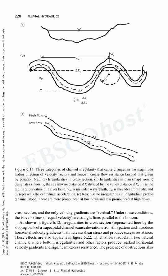
Clearly, any irregularities in channel geometry will cause velocity vectors to deviatefrom direct downstream flow, producing accelerations and concomitant increases inresisting forces. Figure 6.11 shows three categories of geometrical irregularities: incross section, in plan (map) view, and in reach-scale longitudinal profile (slope).These geometrical irregularities are usually the main sources of the excess resistanceapparent in figure 6.10.
6.6.1.1 Cross-section Irregularities
Equation 6.25 gives resistance in hydraulically rough flows in wide open channels inwhich the depth is constant, the P-vK velocity profile applies at all locations in the
Copyright © 2009. Oxford University Press. All rights reserved. May not be reproduced in any form without permission from the publisher, except fair uses permitted under
U.S. or applicable copyright law.
EBSCO Publishing : eBook Academic Collection (EBSCOhost) - printed on 2/19/2017 4:55 PM viaUNIV OF CHICAGOAN: 271150 ; Dingman, S. L..; Fluvial HydraulicsAccount: s8989984
228 FLUVIAL HYDRAULICS
(a)
(b)
rc
ac
ζ ≡ΔXV
ΔXV
λm
αm
ΔX
ΔX
(c) High flow
Low flow
Figure 6.11 Three categories of channel irregularity that cause changes in the magnitudeand/or direction of velocity vectors and hence increase flow resistance beyond that givenby equation 6.25. (a) Irregularities in cross-section. (b) Irregularities in plan (map) view. �
designates sinuosity, the streamwise distance �X divided by the valley distance �Xv; rc is theradius of curvature of a river bend, m is meander wavelength, am is meander amplitude, andac represents the centrifugal acceleration. (c) Reach-scale irregularities in longitudinal profile(channel slope); these are more pronounced at low flows and less pronounced at high flows.
cross section, and the only velocity gradients are “vertical.” Under these conditions,the isovels (lines of equal velocity) are straight lines parallel to the bottom.
As shown in figure 6.12, irregularities in cross section (represented here by thesloping bank of a trapezoidal channel) cause deviations from this pattern and introducehorizontal velocity gradients that increase shear stress and produce excess resistance.These effects are also apparent in figure 5.22, which shows isovels in two naturalchannels, where bottom irregularities and other factors produce marked horizontalvelocity gradients and significant excess resistance. The presence of obstructions also
Copyright © 2009. Oxford University Press. All rights reserved. May not be reproduced in any form without permission from the publisher, except fair uses permitted under
U.S. or applicable copyright law.
EBSCO Publishing : eBook Academic Collection (EBSCOhost) - printed on 2/19/2017 4:55 PM viaUNIV OF CHICAGOAN: 271150 ; Dingman, S. L..; Fluvial HydraulicsAccount: s8989984

UNIFORM FLOW AND FLOW RESISTANCE 229
0.05.0 5.5 6.0 6.5 7.0 7.5 8.0 8.5 9.0 9.5 10.0
0.5
1.0
1.5
2.0
2.5
3.0
Distance from Center, (m)
Elev
atio
n (m
)
1.9 1.0 0.8
Figure 6.12 Isovels in the near-bank portion of an idealized flow in a trapezoidal channel.The P-vK vertical velocity distribution applies at all points; contours are in m/s. Cross-section irregularities, represented here by the sloping bank, induce horizontal velocity gradientsthat increase turbulent shear stress and therefore resistance.
induces secondary circulations and tends to suppress the maximum velocity belowthe surface (see figures 5.17, 5.19, and 5.20), further increasing resistance.
These effects are very difficult to quantify. However, the effects of cross-section irregularity should tend to diminish as depth increases in a particular reach,so at least to some extent these effects are accounted for by the inclusion of therelative smoothness Y/yr in equation 6.25. Apparently, there been no systematicstudies attempting to relate resistance to some measure of the variation of depth ina reach or cross section (e.g., the standard deviation of depth).
Bathurst (1993) reviewed resistance equations for natural streams in which graveland boulders are a major source of cross-section irregularity. For approximatelyuniform flow in gravel-bed streams, he found that resistance could be estimated with±30% error as
� = 0.400·[− ln
(d84
3.60·R)]−1
, (6.27)
for reaches in which 39 mm ≤ d84 ≤ 250 mm and 0.7 ≤ R/d84 ≤ 17. For boulder-bedstreams, Bathurst (1993) suggested the following equation, which is based on datafrom flume and field studies:
� = 0.410·[− ln
(d84
5.15·R)]−1
, (6.28)
for reaches in which 0.004 ≤ S ≤ 0.04 and R/d84 ≤ 10. Note that the form ofequations 6.27 and 6.28 is identical to that of equation 6.25, assuming yr = d84.
Copyright © 2009. Oxford University Press. All rights reserved. May not be reproduced in any form without permission from the publisher, except fair uses permitted under
U.S. or applicable copyright law.
EBSCO Publishing : eBook Academic Collection (EBSCOhost) - printed on 2/19/2017 4:55 PM viaUNIV OF CHICAGOAN: 271150 ; Dingman, S. L..; Fluvial HydraulicsAccount: s8989984

230 FLUVIAL HYDRAULICS
Figure 6.13 shows that excess resistance for gravel and boulder-bed streams givenby equations 6.27 and 6.28 is typically in the range of 20% to well more than 50%.However, it seems surprising that resistance in gravel-bed streams is larger than inboulder-bed streams, and this result may reflect the very imperfect state of knowledgeabout resistance in natural streams, as Bathurst (1993) emphasizes. In some recentstudies, Smart et al. (2002) developed similar relations for use in the relative-roughness range 5 ≤ R/d84 ≤ 20, and Bathurst (2002) recommended computingresistance as a function of R/d84 via the formulas shown in table 6.1 as minimumvalues for resistance in mountain rivers with R/d84 < 11 and 0.002 ≤ S0 ≤ 0.04.
0.00 2 4 6 8 10 12 14 16 18 20
0.1
0.2
0.3
0.4
0.5
0.6
0.7
0.8
0.9
1.0
R/d84
GravelEquation (6.27)
BouldersEquation (6.28)
(Ω −
Ω∗)
/Ω∗
Figure 6.13 Ratio of excess resistance to baseline resistance for gravel and boulder-bedstreams according to Bathurst (1993) (equations 6.27 and 6.28). Values are typically in therange of 20% to well more than 50%.
Table 6.1 Minimum values of resistance recommended by Bathurst(2002) for mountain rivers with R/d84 < 11 and 0.002 ≤ S0 ≤ 0.04.a
Slope range Resistance (�)
0.002 ≤ S0 ≤ 0.008 3.84·(
Y
d84
)0.547
0.008 ≤ S0 ≤ 0.04 3.10·(
Y
d84
)0.93
aThese values apply to situations in which resistance is primarily due to bed roughness;variations in planform, longitudinal profile, vegetation, and so forth, increase � beyond valuesgiven here.
Copyright © 2009. Oxford University Press. All rights reserved. May not be reproduced in any form without permission from the publisher, except fair uses permitted under
U.S. or applicable copyright law.
EBSCO Publishing : eBook Academic Collection (EBSCOhost) - printed on 2/19/2017 4:55 PM viaUNIV OF CHICAGOAN: 271150 ; Dingman, S. L..; Fluvial HydraulicsAccount: s8989984
UNIFORM FLOW AND FLOW RESISTANCE 231
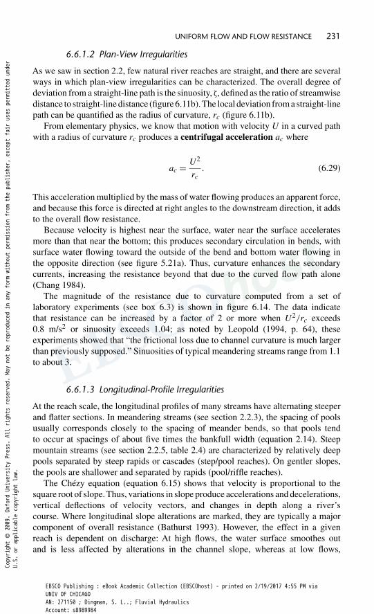
6.6.1.2 Plan-View Irregularities
As we saw in section 2.2, few natural river reaches are straight, and there are severalways in which plan-view irregularities can be characterized. The overall degree ofdeviation from a straight-line path is the sinuosity, �, defined as the ratio of streamwisedistance to straight-line distance (figure 6.11b).The local deviation from a straight-linepath can be quantified as the radius of curvature, rc (figure 6.11b).
From elementary physics, we know that motion with velocity U in a curved pathwith a radius of curvature rc produces a centrifugal acceleration ac where
ac = U2
rc. (6.29)
This acceleration multiplied by the mass of water flowing produces an apparent force,and because this force is directed at right angles to the downstream direction, it addsto the overall flow resistance.
Because velocity is highest near the surface, water near the surface acceleratesmore than that near the bottom; this produces secondary circulation in bends, withsurface water flowing toward the outside of the bend and bottom water flowing inthe opposite direction (see figure 5.21a). Thus, curvature enhances the secondarycurrents, increasing the resistance beyond that due to the curved flow path alone(Chang 1984).
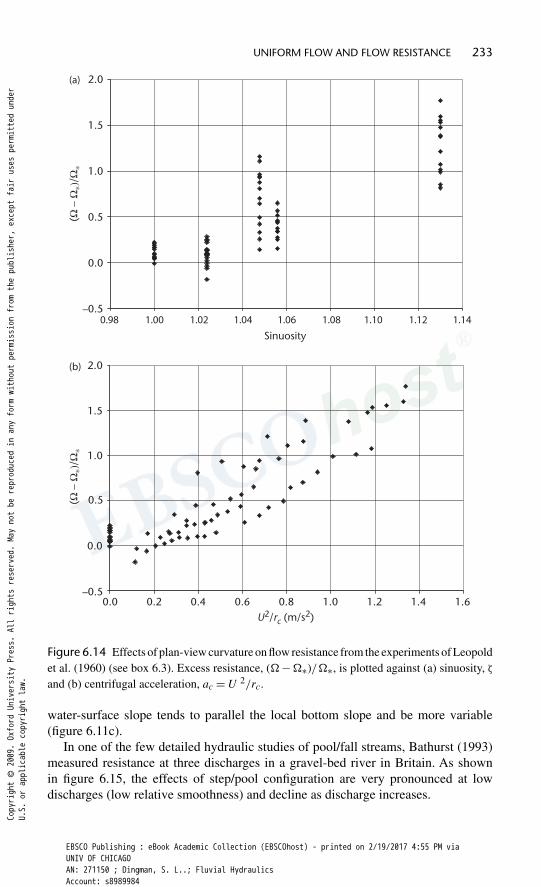
The magnitude of the resistance due to curvature computed from a set oflaboratory experiments (see box 6.3) is shown in figure 6.14. The data indicatethat resistance can be increased by a factor of 2 or more when U2/rc exceeds0.8 m/s2 or sinuosity exceeds 1.04; as noted by Leopold (1994, p. 64), theseexperiments showed that “the frictional loss due to channel curvature is much largerthan previously supposed.” Sinuosities of typical meandering streams range from 1.1to about 3.
6.6.1.3 Longitudinal-Profile Irregularities
At the reach scale, the longitudinal profiles of many streams have alternating steeperand flatter sections. In meandering streams (see section 2.2.3), the spacing of poolsusually corresponds closely to the spacing of meander bends, so that pools tendto occur at spacings of about five times the bankfull width (equation 2.14). Steepmountain streams (see section 2.2.5, table 2.4) are characterized by relatively deeppools separated by steep rapids or cascades (step/pool reaches). On gentler slopes,the pools are shallower and separated by rapids (pool/riffle reaches).
The Chézy equation (equation 6.15) shows that velocity is proportional to thesquare root of slope. Thus, variations in slope produce accelerations and decelerations,vertical deflections of velocity vectors, and changes in depth along a river’scourse. Where longitudinal slope alterations are marked, they are typically a majorcomponent of overall resistance (Bathurst 1993). However, the effect in a givenreach is dependent on discharge: At high flows, the water surface smoothes outand is less affected by alterations in the channel slope, whereas at low flows,
Copyright © 2009. Oxford University Press. All rights reserved. May not be reproduced in any form without permission from the publisher, except fair uses permitted under
U.S. or applicable copyright law.
EBSCO Publishing : eBook Academic Collection (EBSCOhost) - printed on 2/19/2017 4:55 PM viaUNIV OF CHICAGOAN: 271150 ; Dingman, S. L..; Fluvial HydraulicsAccount: s8989984

BOX 6.3 Flume Experiments on Resistance in Sinuous Channels
Leopold et al. (1960) conducted a series of experiments in a tiltable flumewith a length of 15.9 m. Sand with a median diameter of 2 mm was placed inthe flume, and a template was designed that could mold straight or curvedtrapezoidal channels in the sand. Once the channels were molded, theywere coated with adhesive to prevent erosion. Plan-view geometries were asin table 6B3.1.
Table 6B3.1
Wavelength (m) Radius of curvature rc (m) Sinuosity �
Straight Straight 1.0001.22 1.01 1.0241.18 0.58 1.0560.65 0.31 1.0480.70 0.19 1.130
Flows were run at two depths; cross-section geometries were as intable 6B3.2.
Table 6B3.2
MaximumdepthYm(m)
BottomwidthWb(m)
Water-surfacewidthW (m)
AveragedepthY (m)
Cross-sectionalarea A (m2)
WettedperimeterPw (m)
HydraulicradiusR (m)
0.027 0.117 0.191 0.020 0.00418 0.209 0.0200.041 0.117 0.224 0.027 0.00697 0.252 0.028
For each run, slope (S) and discharge (Q) could be set to obtain constantdepth (uniform flow) throughout. The ranges of velocities (U), Reynoldsnumbers (Re) and Froude numbers (Fr ) observed are listed in table 6B3.3.
Table 6B3.3
S Q (m3/s) U (m/s) Re Fr
Maximum 0.0118 0.00326 0.466 12100 0.970Minimum 0.00033 0.00048 0.097 2130 0.187
The results of these experiments were used to plot figure 6.14 and gainquantitative insight on the effects of curvature on resistance.
232
Copyright © 2009. Oxford University Press. All rights reserved. May not be reproduced in any form without permission from the publisher, except fair uses permitted under
U.S. or applicable copyright law.
EBSCO Publishing : eBook Academic Collection (EBSCOhost) - printed on 2/19/2017 4:55 PM viaUNIV OF CHICAGOAN: 271150 ; Dingman, S. L..; Fluvial HydraulicsAccount: s8989984
UNIFORM FLOW AND FLOW RESISTANCE 233
–0.5
0.0
0.5
1.0
1.5
2.0
Sinuosity
0.98 1.00 1.02 1.04 1.06 1.08 1.10 1.12 1.14
(Ω
− Ω
∗)/Ω
∗
–0.50.0 0.2 0.4 0.6 0.8 1.0 1.2 1.4 1.6
0.0
0.5
1.0
1.5
2.0
(Ω
− Ω
∗)/Ω
∗
U2/rc (m/s2)
(a)
(b)
Figure 6.14 Effects of plan-view curvature on flow resistance from the experiments of Leopoldet al. (1960) (see box 6.3). Excess resistance, (�−�∗)/�∗, is plotted against (a) sinuosity, �
and (b) centrifugal acceleration, ac = U 2/rc.
water-surface slope tends to parallel the local bottom slope and be more variable(figure 6.11c).
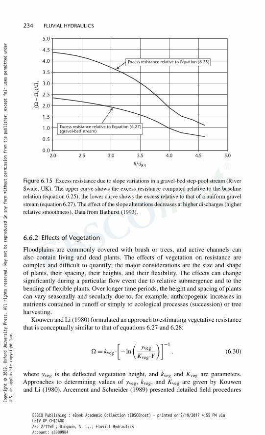
In one of the few detailed hydraulic studies of pool/fall streams, Bathurst (1993)measured resistance at three discharges in a gravel-bed river in Britain. As shownin figure 6.15, the effects of step/pool configuration are very pronounced at lowdischarges (low relative smoothness) and decline as discharge increases.
Copyright © 2009. Oxford University Press. All rights reserved. May not be reproduced in any form without permission from the publisher, except fair uses permitted under
U.S. or applicable copyright law.
EBSCO Publishing : eBook Academic Collection (EBSCOhost) - printed on 2/19/2017 4:55 PM viaUNIV OF CHICAGOAN: 271150 ; Dingman, S. L..; Fluvial HydraulicsAccount: s8989984
234 FLUVIAL HYDRAULICS
0.0
0.5
1.0
1.5
2.0
2.5
3.0
3.5
4.0
4.5
5.0
R/d84
Excess resistance relative to Equation (6.25)
Excess resistance relative to Equation (6.27)(gravel-bed stream)
(Ω
− Ω
∗)/Ω
∗
2.0 2.5 3.0 3.5 4.0 4.5 5.0
Figure 6.15 Excess resistance due to slope variations in a gravel-bed step-pool stream (RiverSwale, UK). The upper curve shows the excess resistance computed relative to the baselinerelation (equation 6.25); the lower curve shows the excess relative to that of a uniform gravelstream (equation 6.27). The effect of the slope alterations decreases at higher discharges (higherrelative smoothness). Data from Bathurst (1993).
6.6.2 Effects of Vegetation
Floodplains are commonly covered with brush or trees, and active channels canalso contain living and dead plants. The effects of vegetation on resistance arecomplex and difficult to quantify; the major considerations are the size and shapeof plants, their spacing, their heights, and their flexibility. The effects can changesignificantly during a particular flow event due to relative submergence and to thebending of flexible plants. Over longer time periods, the height and spacing of plantscan vary seasonally and secularly due to, for example, anthropogenic increases innutrients contained in runoff or simply to ecological processes (succession) or treeharvesting.
Kouwen and Li (1980) formulated an approach to estimating vegetative resistancethat is conceptually similar to that of equations 6.27 and 6.28:
� = kveg·[− ln
(yveg
Kveg·Y)]−1
, (6.30)
where yveg is the deflected vegetation height, and kveg and Kveg are parameters.Approaches to determining values of yveg, kveg, and Kveg are given by Kouwenand Li (1980). Arcement and Schneider (1989) presented detailed field procedures
Copyright © 2009. Oxford University Press. All rights reserved. May not be reproduced in any form without permission from the publisher, except fair uses permitted under
U.S. or applicable copyright law.
EBSCO Publishing : eBook Academic Collection (EBSCOhost) - printed on 2/19/2017 4:55 PM viaUNIV OF CHICAGOAN: 271150 ; Dingman, S. L..; Fluvial HydraulicsAccount: s8989984

UNIFORM FLOW AND FLOW RESISTANCE 235
0.03020000 40000 60000 80000 100000 120000 140000 160000 1800000
0.035
0.040
0.045
0.050
0.055
Re
Ω
Equation (6.25)
Fr > 3.5
Figure 6.16 Plot of flow resistance, �, versus Reynolds number, Re, showing the effect ofsurface instability on flow resistance. The curve is the standard resistance relation for smoothchannels given in equation 6.25; the points are resistance values measured in flume experimentsof Sarma and Syala (1991). The points clustering close to the curve have 1 < Fr < 3.5; thoseplotting substantially above the curve have Fr > 3.5.
for estimating resistance due to vegetation on floodplains. Recent analyses andexperiments evaluating resistance due to vegetation are given by Wilson and Horritt(2002) and Rose et al. (2002) and summarized by Yen (2002).
6.6.3 Effects of Surface Instability
As noted in section 6.2.2.2, wavelike fluctuations begin to appear in the surfacesof open-channel flows as the Froude number Fr approaches 1. A few experi-mental studies in flumes have examined the effects of these instabilities on flowresistance.
Figure 6.16 summarizes measurements of supercritical flows in a straight, smooth,rectangular flume (Sarma and Syala 1991). It shows that for flows with 1 <
Fr < 3.5, flow resistance is essentially as predicted by the standard relation forsmooth turbulent flows (equation 6.25). However, when Fr exceeds a thresholdvalue of about 3.5, there is a discontinuity, and resistance jumps to a valueabout 10% larger than the standard value. Because Froude numbers in naturalchannels seldom exceed 1, Sarma and Syala’s (1991) results suggest that one canusually safely ignore the effects of surface instabilities on resistance in straightchannels.
However, the experiments of Leopold et al. (1960) described in box 6.3 indicate theexistence of discontinuities in resistance that they attributed to surface instabilities
Copyright © 2009. Oxford University Press. All rights reserved. May not be reproduced in any form without permission from the publisher, except fair uses permitted under
U.S. or applicable copyright law.
EBSCO Publishing : eBook Academic Collection (EBSCOhost) - printed on 2/19/2017 4:55 PM viaUNIV OF CHICAGOAN: 271150 ; Dingman, S. L..; Fluvial HydraulicsAccount: s8989984

236 FLUVIAL HYDRAULICS
at channel bends and called spill resistance. These sudden increases in resistanceoccurred at Froude numbers in the range of 0.4−0.55, much lower than found bySarma and Syala (1991) in straight smooth flumes. Thus, spill resistance may bea significant contributor to excess resistance at high flows in channel bends.
6.6.4 Effects of Sediment
Sediment transport affects flow resistance in two principal ways: 1) the effects ofsuspended sediment on turbulence characteristics, and 2) the effects of bedforms thataccompany sediment transport on channel-bed configuration.
6.6.4.1 Effects of Sediment Load
As noted in section 5.3.1.4, there is evidence that suspended sediment suppressesturbulence and causes the value of von Kármán’s constant, �, to decrease belowits clear-water value of � = 0.4. Evidence analyzed by Einstein and Chien (1954)suggested values as low as � = 0.2 at high sediment concentrations. Because thecoefficient in equation 6.25 is �, this suggests that resistance could be as little as 50%of its clear-water value in flows transporting sediment.
However, some researchers contend that � remains constant and the observedresistance reduction in flows transporting sediment is due to an altered velocitydistribution such that, in sediment-laden flows, velocities near the bed are reducedand those near the surface increased compared with the values given by the P-vKlaw (Coleman 1981; Lau 1983). Other studies have even suggested that resistance isgenerally increased sediment-laden flows compared with clear-water flows underidentical conditions (Lyn 1991). Clearly this is a question that requires furtherresearch.
6.6.4.2 Effects of Bedforms
Observations of rivers and experiments in flumes (e.g., Simons and Richardson1966) have revealed that in flows over sand beds, there is a typical sequence ofbedforms that occurs as discharge changes. These forms are intimately related toprocesses of erosion that begin when the critical value of boundary shear stress, �0, isreached,7 and in turn they strongly affect the velocity because of their effects on flowresistance.
The bedforms are described and illustrated in table 6.2 and figures 6.17–6.19,and figure 6.20 shows qualitatively how resistance changes through the sequence. Ingeneral, resistance increases directly with bedform height (amplitude) and inverselywith bedform wavelength.
Bathurst (1993) developed an approach to accounting for these effects that involvescomputing the effective roughness height of the bedforms, ybf, as a function of grainsize, d84; bedform amplitude, Abf; and bedform wavelength, bf:
ybf = 3 · d84 + 1.1 · Abf · [1 − exp(−25 · Abf/bf)] (6.31)
Copyright © 2009. Oxford University Press. All rights reserved. May not be reproduced in any form without permission from the publisher, except fair uses permitted under
U.S. or applicable copyright law.
EBSCO Publishing : eBook Academic Collection (EBSCOhost) - printed on 2/19/2017 4:55 PM viaUNIV OF CHICAGOAN: 271150 ; Dingman, S. L..; Fluvial HydraulicsAccount: s8989984

Table 6.2 Bedforms in sand-bed streams (see figures 6.17–6.20).
MigrationBedform Description Amplitude Wavelength velocity (mm/s) �bf
Lower flowregime, Fr < 1
Plane bed Generally flat bed, often with irregularities due todeposition; occurs in absence of erosion.
0.05–0.06
Ripples Small wavelike bedforms; may be triangular tosinusoidal in longitudinal cross section. Crests aretransverse to flow and may be short and irregular tolong, parallel, regular ridges; typically migratedownstream at velocities much lower than streamvelocity; may occur on upslope portions of dunes.
< 40 mm; mostly10–20 mm
< 60 mm 0.1–1 0.07–0.1
Dunes Larger wavelike forms with crests transverse to flow,out of phase with surface waves; generally triangularin longitudinal cross section with gentle upstreamslopes and steep downstream slopes. Crest lengths areapproximately same magnitude as wavelength;migrate downstream at velocities much lower thanstream velocity.
0.1–10 m; usually≈ 0.1 × Y to0.3 × Y
0.1–100 m,usually ≈ 2 × Yto 10 × Y
0.1–1 0.07–0.14
Upper flowregime, Fr > 1
Plane bed Often occurs with heterogeneous, irregular forms;a mixture of flat areas and low-amplitude ripplesand/or dunes.
< 3 mm Irregular 10 0.05–0.06
Antidunes Large wavelike forms with triangular to sinusoidallongitudinal cross sections that are in phase withwater-surface waves. Crest lengths approximatelyequal wavelength; may migrate upstream ordownstream or remain stationary.
30–100 mm 2· ·Y Variable 0.05–0.06
Chutes and pools Large mounds of sediment that form steep chutes inwhich flow is supercritical, separated by pools inwhich flow may be subcritical or supercritical.Hydraulic jumps (see chapter 10) form atsupercritical-to-subcritical transitions; migrate slowlyupstream.
1–50
After Task Force on Bed Forms in Alluvial Channels (1966) and Bridge (2003).
237
Copyright © 2009. Oxford University Press. All rights reserved. May not be reproduced in any form without permission from the publisher,
except fair uses permitted under U.S. or applicable copyright law.
EBSCO Publishing : eBook Academic Collection (EBSCOhost) - printed on 2/19/2017 4:55 PM via UNIV OF CHICAGOAN: 271150 ; Dingman, S. L..; Fluvial HydraulicsAccount: s8989984

238 FLUVIAL HYDRAULICS
(a)
(b)
Figure 6.17 Ripples. (a) Side view of ripples in a laboratory flume. The flow is from left toright at a mean depth of 0.064 m and a mean velocity of 0.43 m/s (Fr = 0.54). Aluminumpowder was added to the water to make the flow paths visible. Note that the water surfaceis unaffected by the ripples. Photograph courtesy of A. V. Jopling, University of Toronto. (b)Ripples on the bed of the Delta River in central Alaska. Flow was from left to right.
Resistance is then computed as
� = 0.400 ·[− ln
( ybf
12.1·R)]−1
, (6.32)
where R is hydraulic radius (≈ Y for wide channels).In another approach, the resistance is separated into 1) that due to the bed
material (the plane-bed resistance �∗ given by equation 6.25) and 2) that due tothe bedforms, �bf:
� = �∗ +�bf. (6.33)
Copyright © 2009. Oxford University Press. All rights reserved. May not be reproduced in any form without permission from the publisher, except fair uses permitted under
U.S. or applicable copyright law.
EBSCO Publishing : eBook Academic Collection (EBSCOhost) - printed on 2/19/2017 4:55 PM viaUNIV OF CHICAGOAN: 271150 ; Dingman, S. L..; Fluvial HydraulicsAccount: s8989984

UNIFORM FLOW AND FLOW RESISTANCE 239
(a)
(b)
Figure 6.18 Dunes. (a) Side view of dunes in a laboratory flume. The flow is from left toright at a mean depth of 0.064 m and a mean velocity of 0.67 m/s (Fr = 0.85). Aluminumpowder was added to the water to make the flow paths visible. Note that the water surface isout of phase with the bedforms. Photograph courtesy of A.V. Jopling, University of Toronto.(b) Dunes in a laboratory flume. Flow was toward the observer at a mean depth of 0.31 m and amean velocity of 0.85 m/s (Fr = 0.49). Note ripples superimposed on some dunes. Photographcourtesy of D.B. Simons, Colorado State University.
Yen (2002) reviews several approaches to estimating �bf; some typical values areindicated in table 6.2.
6.6.5 Effects of Ice
As noted in section 3.2.2.3, the presence of an ice cover or frazil ice can significantlyincrease resistance. For a uniform flow in a rectangular channel (figure 6.7), the effect
Copyright © 2009. Oxford University Press. All rights reserved. May not be reproduced in any form without permission from the publisher, except fair uses permitted under
U.S. or applicable copyright law.
EBSCO Publishing : eBook Academic Collection (EBSCOhost) - printed on 2/19/2017 4:55 PM viaUNIV OF CHICAGOAN: 271150 ; Dingman, S. L..; Fluvial HydraulicsAccount: s8989984

240 FLUVIAL HYDRAULICS
Figure 6.19 Side view of antidunes in a laboratory flume The flow is from left to right ata mean depth of 0.11 m and a mean velocity of 0.79 m/s (Fr = 0.76). Note that the surfacewaves are approximately in phase with the bedforms, which are also migrating to the right.Photograph courtesy of J. F. Kennedy, University of Iowa.
BED FORM
STREAM POWER
Lower regime
Bed
Plain bed Ripples Dunes Transition Plain bed Standing wavesand antidunes
Watersurface
Transition Upper regime
Resistance to flow(Manning’s roughnesscoefficient)
Figure 6.20 Sequence of bedforms and flow resistance in sand-bed streams. From Arcementand Schneider (1989). See table 6.2 for typical � values.
of an ice cover can be included in formulating the expression for the resisting forces,so that equation 6.10 becomes
FR = �B·(2·Y + W )·X + �I ·W ·X, (6.34)
where �B is the shear stress on the bed and �I is the shear stress on the ice cover. If thisforce balances the downstream-directed force (equation 6.7) and we assume a widechannel (i.e., Pw = W ), the modified Chézy equation becomes
U = (�2B +�2
I )−1/2·u∗, (6.35)
where �B and �I are the resistances due to the bed and the ice cover, respectively.One would expect �I to vary widely in natural streams due to 1) variations in
the degree of ice cover, 2) development of ripplelike and dunelike bedforms on theunderside of the ice cover (Ashton and Kennedy 1972), 3) development of partial orcomplete ice jamming, and 4) the concentration of frazil ice in the flow. An analysisof ice resistance on the St. Lawrence River by Tsang (1982) indicates that �I is on
Copyright © 2009. Oxford University Press. All rights reserved. May not be reproduced in any form without permission from the publisher, except fair uses permitted under
U.S. or applicable copyright law.
EBSCO Publishing : eBook Academic Collection (EBSCOhost) - printed on 2/19/2017 4:55 PM viaUNIV OF CHICAGOAN: 271150 ; Dingman, S. L..; Fluvial HydraulicsAccount: s8989984

UNIFORM FLOW AND FLOW RESISTANCE 241
the order of 0.7−1.5 times �B, and data presented by Chow (1959) suggest values inthe range from �I = 0.03 for smooth ice without ice blocks to �I = 0.085 for roughice with ice blocks. White (1999) and Brunner (2001b) summarized resistance due toice given by several studies; these cover a very wide range of values.
6.7 Field Computation of Reach Resistance
Validation of methods of determining reach resistance requires comparison withactual resistance values. The method developed here to compute resistance in natural,nonprismatic channels is based closely on the concepts used to derive the Chézyequation for uniform flow in prismatic channels in section 6.3.
Designating X as the distance measured along the stream course, the cross-sectional area, A, wetted perimeter, Pw, hydraulic radius, R, and water-surfaceslope, SS , vary through a natural-channel reach (figure 6.21) and so are written asfunctions of X: A(X), Pw(X), R(X), and SS(X) respectively. With this notation, thedownstream-directed force, FD, is
FD = �·∫ XN
X0
A(X)·SS(X)·dX, (6.36)
where X0 and XN are the locations of the upstream and downstream boundaries ofthe reach, respectively. Note that this expression is analogous to equation 6.7, but fornonprismatic rather than prismatic channels.
Similarly, the upstream-directed resistance force, FR in a nonprismatic channel is
FR = KT ·�·U2·∫ XN
X0
Pw(X)·dX, (6.37)
where U is the reach-average velocity. This expression is analogous to equation 6.10.For a given discharge, Q, the reach-average velocity is
U = Q(1
�X
)·∫ XN
X0A(X)·dX
. (6.38)
where �X ≡ XN − X0.Equating FD and FR as in equation 6.6, substituting equations 6.36–6.38, and
solving for KT gives
KT =g·∫ XN
X0A(X)·SS(X)·dX ·
[∫ XNX0
A(X)·dX]2
Q2·�X2·∫ XNX0
Pw(X)·dX= �2; (6.39a)
� =g1/2·
[∫ XNX0
A(X)·SS(X)·dX]1/2 ·∫ XN
X0A(X)·dX
Q·�X·[∫ XN
X0 Pw(X)·dX]1/2
. (6.39b)
Copyright © 2009. Oxford University Press. All rights reserved. May not be reproduced in any form without permission from the publisher, except fair uses permitted under
U.S. or applicable copyright law.
EBSCO Publishing : eBook Academic Collection (EBSCOhost) - printed on 2/19/2017 4:55 PM viaUNIV OF CHICAGOAN: 271150 ; Dingman, S. L..; Fluvial HydraulicsAccount: s8989984

242 FLUVIAL HYDRAULICS
PLAN SKETCH1
2 3 4 56
7
1
1
2
15
10
5
0
15
10
5
0
15
10
5
0
ELEV
ATIO
N IN
FEE
T, G
AG
E D
ATU
M
15
10
5
0
3
3
45
5
11816
7
7
CROSS SECTIONS
Water surface 12/28/58
1180
–50 40 80 120 160 200 240 280
WIDTH, IN FEET
Figure 6.21 Plan view and cross sections of the Deep River at Ramseur, North Carolina,showing typical cross-section variability. From Barnes (1967).
In practice, the geometric functions A(X), SS(X), and so on, can be approximatedonly by measurements at specific cross sections within the reach. Thus. for practicalapplication, equation 6.39b becomes
� =g1/2·
[N∑
i = 1Ai·SSi·�Xi
]1/2
·N∑
i = 1Ai·�Xi
Q·�X·[
N∑i = 1
Pwi·�Xi
]1/2, (6.39c)
where the subscripts indicate the measured value of the variable at cross section i, i =1,2, . . .,N , and �Xi is the downstream distance between successive cross sections.
Copyright © 2009. Oxford University Press. All rights reserved. May not be reproduced in any form without permission from the publisher, except fair uses permitted under
U.S. or applicable copyright law.
EBSCO Publishing : eBook Academic Collection (EBSCOhost) - printed on 2/19/2017 4:55 PM viaUNIV OF CHICAGOAN: 271150 ; Dingman, S. L..; Fluvial HydraulicsAccount: s8989984

UNIFORM FLOW AND FLOW RESISTANCE 243
Box 6.4 shows how field computations are used to compute resistance. It isimportant to be aware that careful field measurements are essential for accuratehydraulic computations. The manual by Harrelson et al. (1994) is an excellentillustrated guide to field technique.
6.8 The Manning Equation
6.8.1 Origin
In the century following the publication of the Chézy equation in 1769, Europeanhydraulic engineers did considerable field and laboratory research to develop practicalways to estimate open-channel flow resistance (Rouse and Ince 1963; Dooge 1992).In 1889, Robert Manning (1816–1897), an Irish engineer, published an extensivereview of that research (Manning 1889). He concluded that the simple equation thatbest fit the experimental results was
U = KM ·R2/3·S1/2S , (6.40a)
where KM is a proportionality constant representing reach conductance. For historicalreasons (see Dooge 1992), subsequent researchers replaced KM by its inverse, 1/nM ,and wrote the equation as
U =(
1
nM
)·R2/3·S1/2
S , (6.40b)
called Manning’s equation, where the resistance factor nM is calledManning’s n.
Manning’s equation has come to be accepted as “the” resistance equation foropen-channel flow, largely replacing the Chézy equation in practical applications.The essential difference between the two is that the hydraulic-radius exponent is2/3 rather than 1/2. This difference is important because it makes the Manningequation dimensionally inhomogeneous.8 As with Chézy’s C (see box 6.1), values ofnM are treated as constants for all unit systems, and in order to give correct results,the Manning equation must be written as
U = uM ·(
1
nM
)·R2/3·S1/2, (6.40c)
where uM is a unit-adjustment factor that takes the following values:
Unit system uM
Système Internationale 1.00British 1.49Centimeter-gram-second 4.64
Copyright © 2009. Oxford University Press. All rights reserved. May not be reproduced in any form without permission from the publisher, except fair uses permitted under
U.S. or applicable copyright law.
EBSCO Publishing : eBook Academic Collection (EBSCOhost) - printed on 2/19/2017 4:55 PM viaUNIV OF CHICAGOAN: 271150 ; Dingman, S. L..; Fluvial HydraulicsAccount: s8989984
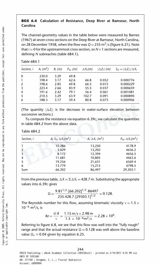
BOX 6.4 Calculation of Resistance, Deep River at Ramseur, NorthCarolina
The channel-geometry values in the table below were measured by Barnes(1967) at seven cross sections on the Deep River at Ramseur, North Carolina,on 28 December 1958, when the flow was Q = 235 m3/s (figure 6.21). Notethat i = 0 for the upstreammost cross section, so N+1 sections are measured,defining N subreaches (table 6B4.1).
Table 6B4.1
Section, i Ai (m2) Ri (m) Pwi (m) �Xi (m) |�Zi | (m) SSi = |�Zi |/�Xi
0 230.0 3.29 69.81 198.4 3.17 62.6 66.8 0.052 0.0007762 198.6 2.85 69.8 66.5 0.015 0.0002293 223.4 2.66 83.9 55.5 0.037 0.0006594 191.6 2.42 79.1 56.4 0.061 0.0010815 210.5 3.29 63.9 102.7 0.091 0.0008906 188.3 3.17 59.4 80.8 0.073 0.000906
(The quantity |�Zi | is the decrease in water-surface elevation betweensuccessive sections.)
To compute the resistance via equation 6.39c, we calculate the quantitiesin table 6B4.2 from the above data.
Table 6B4.2
Section, i Ai ·SSi ·�Xi (m3) Ai ·�Xi (m3) Pwi ·�Xi (m3)
1 10.286 13,250 4178.92 3.029 13,202 4636.23 8.172 12,394 4656.54 11.681 10,805 4463.65 19.256 21,631 6569.46 13.779 15,215 4798.5Sum 66.202 86,497 29,303.1
From the previous table, �X =��Xi =428.7 m. Substituting the appropriatevalues into 6.39c gives
� = 9.811/2· [66.202]1/2 ·86497
235·428.7· [29303.1]1/2 = 0.128.
The Reynolds number for this flow, assuming kinematic viscosity � = 1.5 ×10⁻⁶ m2/s, is
Re = U·R�
= 1.15 m/s ×2.98 m1.5 × 10−6m2/s
= 2.28×10⁶.
Referring to figure 6.8, we see that this flow was well into the “fully rough”range and that the actual resistance � = 0.128 was well above the baselinevalue �∗ ≈ 0.04 given by equation 6.25.
244
Copyright © 2009. Oxford University Press. All rights reserved. May not be reproduced in any form without permission from the publisher, except fair uses permitted under
U.S. or applicable copyright law.
EBSCO Publishing : eBook Academic Collection (EBSCOhost) - printed on 2/19/2017 4:55 PM viaUNIV OF CHICAGOAN: 271150 ; Dingman, S. L..; Fluvial HydraulicsAccount: s8989984

UNIFORM FLOW AND FLOW RESISTANCE 245
From equations 6.12, 6.19, 6B1.3, and 6.40c, we see that
nM = uM ·R1/6·K1/2T
g1/2= uM ·R1/6
uC ·C = uM ·R1/6·�g1/2
. (6.41)
A major justification for using the Manning equation instead of the Chézyequation has been that, because nM depends on the hydraulic radius, it accountsfor relative submergence effects and tends to be more constant for a given reach(i.e., changes less as discharge changes) than is C. However, this reasoning may notbe compelling, because we have seen that we can write the Chézy equation using�−1 instead of uC ·C (equation 6.19) and that �, in fact, depends in large measureon relative submergence (equation 6.24). Another reason for the popularity of theManning equation is that a number of methods have been developed that provideexpedient (i.e., “quick-and-dirty”) estimates of the resistance coefficient nM . Thesemethods are discussed in the following section.
6.8.2 Determination of Manning’s nM
In order to apply the Manning equation in practical problems, one must be able todetermine a priori values of nM . An overview of approaches to doing this are listedin table 6.3 and briefly described in the following subsections.
6.8.2.1 Visual Comparison with Photographs
Table 6.4 summarizes publications that provide guidance for field determination ofnM by means of photographs of reaches in which nM values have been determinedby measurement for one or more discharges. The books by Barnes (1967) and Hicksand Mason (1991) are specifically designed to provide visual guidance for the fielddetermination of nM for in-bank flows in natural rivers. Examples from Barnes (1967)are shown in figure 6.22.
6.8.2.2 Tables of Typical nM Values
Chow (1959) provides tables that give a range of appropriate nM values for varioustypes of human-made canals and natural channels; the portions of those tablescovering natural channels are reproduced here in table 6.5.
6.8.2.3 Formulas That Account for Components ofReach Resistance
Cowan (1956) introduced a formula that allowed for explicit consideration of manyof the factors that determine resistance (see section 6.6) in determining an appropriatenM value:
nM = (n0 + n1 + n2 + n3 + n4)·m�, (6.42)
where n0 is the base value for straight, uniform, smooth channel in naturalmaterial; n1 is the factor for bed and bank roughness; n2 is the factor for effect of
Copyright © 2009. Oxford University Press. All rights reserved. May not be reproduced in any form without permission from the publisher, except fair uses permitted under
U.S. or applicable copyright law.
EBSCO Publishing : eBook Academic Collection (EBSCOhost) - printed on 2/19/2017 4:55 PM viaUNIV OF CHICAGOAN: 271150 ; Dingman, S. L..; Fluvial HydraulicsAccount: s8989984

Table 6.3 General approaches to a priori estimation of Manning’s nM .
Approach Comments References
1. Visual comparison withphotographs of channelsfor which nM has beenmeasured (see table 6.4)
Expedient method; subjective, dependent onoperator experience; subject toconsiderable uncertainty
Faskin (1963), Barnes(1967), Arcement andSchneider (1989),Hicks and Mason(1991)
2. Tables of typical nM
values for reaches ofvarious materials andtypes (see table 6.5)
Expedient method; subjective, dependent onoperator experience; subject toconsiderable uncertainty
Chow (1959), French(1985)
3. Formulas that account forcomponents of reachresistance (see table 6.6)
Expedient method; more objective thanapproaches 1 and 2 but lacks theoreticalbasis
Cowan (1956), Faskin(1963), Arcement andSchneider (1989)
4. Formulas that relate nM tobed-sediment grain size dp
(see table 6.7)
Require measurement of bed sediment;reliable only for straight quasi-prismaticchannels where bed roughness is thedominant factor contributing to resistance
Chang (1988), Marcuset al. (1992)
5. Formulas that relate nM tohydraulic radius andrelative smoothness
Require measurement of bed sediment,depth, and slope; forms are based ontheory; coefficients are based on fieldmeasurement; can give good results inconditions similar to those for whichestablished
Limerinos (1970),Bathurst (1985)
6. Statistical formulas thatrelate nM to measurableflow parameters(see table 6.8)
Can provide good estimates, especiallyuseful when bed-material information islacking, as in remote sensing, but subjectto considerable uncertainty
Riggs (1976), Jarrett(1984), Dingman andSharma (1997),Bjerklie et al. (2003)
Table 6.4 Summary of reports presenting photographs of reaches for which Manning’s nM
has been measured.
Types of reach No. of reaches No. of flows Minimum nM Maximum nM Reference
Canals anddredgedchannels (USA)
48 326 0.014 0.162 Faskin (1963)
Natural rivers(USA)
51 62 0.024 0.075 Barnes (1967)
Flood plains(USA)
16 16 —a —a Arcement andSchneider(1989)
Natural rivers(New Zealand)
78 559 0.016 0.270 Hicks and Mason(1991)
a See reference for methodology for computing composite (channel plus flood plain) nM values.
246
Copyright © 2009. Oxford University Press. All rights reserved. May not be reproduced in any form without permission from the publisher, except fair uses permitted under
U.S. or applicable copyright law.
EBSCO Publishing : eBook Academic Collection (EBSCOhost) - printed on 2/19/2017 4:55 PM viaUNIV OF CHICAGOAN: 271150 ; Dingman, S. L..; Fluvial HydraulicsAccount: s8989984

(a) (b)
(c) (d)
(e) (f)
(g) (h)
Figure 6.22 Photographs of U.S. river reaches covering a range of values of Manning’s nM ,computed from measurements. (a) Columbia River at Vernita, Washington: nM = 0.024; (b)West Fork Bitterroot River near Conner, Montana: nM = 0.036; c) Moyie River at Eastport,Idaho: nM = 0.038; (d) Tobesofkee Creek near Macon, Georgia: nM = 0.041; (e) Grande RondeRiver at La Grande, Oregon: nM = 0.043; (f) Clear Creek near Golden, Colorado: nM = 0.050;(g) Haw River near Benaja, North Carolina: nM = 0.059; (h) Boundary Creek near Porthill,Idaho: nM = 0.073. From Barnes (1967); photographs courtesy U.S. Geological Survey.
247
Copyright © 2009. Oxford University Press. All rights reserved. May not be reproduced in any form without permission from the publisher, except fair uses permitted under
U.S. or applicable copyright law.
EBSCO Publishing : eBook Academic Collection (EBSCOhost) - printed on 2/19/2017 4:55 PM viaUNIV OF CHICAGOAN: 271150 ; Dingman, S. L..; Fluvial HydraulicsAccount: s8989984
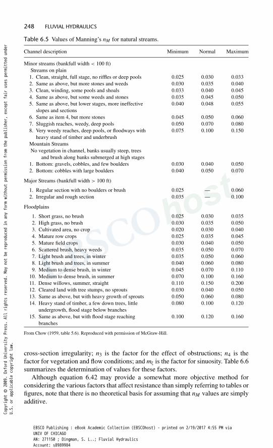
248 FLUVIAL HYDRAULICS
Table 6.5 Values of Manning’s nM for natural streams.
Channel description Minimum Normal Maximum
Minor streams (bankfull width < 100 ft)Streams on plain1. Clean, straight, full stage, no riffles or deep pools 0.025 0.030 0.0332. Same as above, but more stones and weeds 0.030 0.035 0.0403. Clean, winding, some pools and shoals 0.033 0.040 0.0454. Same as above, but some weeds and stones 0.035 0.045 0.0505. Same as above, but lower stages, more ineffective
slopes and sections0.040 0.048 0.055
6. Same as item 4, but more stones 0.045 0.050 0.0607. Sluggish reaches, weedy, deep pools 0.050 0.070 0.0808. Very weedy reaches, deep pools, or floodways with
heavy stand of timber and underbrush0.075 0.100 0.150
Mountain StreamsNo vegetation in channel, banks usually steep, trees
and brush along banks submerged at high stages1. Bottom: gravels, cobbles, and few boulders 0.030 0.040 0.0502. Bottom: cobbles with large boulders 0.040 0.050 0.070
Major Streams (bankfull width > 100 ft)
1. Regular section with no boulders or brush 0.025 — 0.0602. Irregular and rough section 0.035 — 0.100
Floodplains
1. Short grass, no brush 0.025 0.030 0.0352. High grass, no brush 0.030 0.035 0.0503. Cultivated area, no crop 0.020 0.030 0.0404. Mature row crops 0.025 0.035 0.0455. Mature field crops 0.030 0.040 0.0506. Scattered brush, heavy weeds 0.035 0.050 0.0707. Light brush and trees, in winter 0.035 0.050 0.0608. Light brush and trees, in summer 0.040 0.060 0.0809. Medium to dense brush, in winter 0.045 0.070 0.110
10. Medium to dense brush, in summer 0.070 0.100 0.16011. Dense willows, summer, straight 0.110 0.150 0.20012. Cleared land with tree stumps, no sprouts 0.030 0.040 0.05013. Same as above, but with heavy growth of sprouts 0.050 0.060 0.08014. Heavy stand of timber, a few down trees, little
undergrowth, flood stage below branches0.080 0.100 0.120
15. Same as above, but with flood stage reachingbranches
0.100 0.120 0.160
From Chow (1959, table 5.6). Reproduced with permission of McGraw-Hill.
cross-section irregularity; n3 is the factor for the effect of obstructions; n4 is thefactor for vegetation and flow conditions; and m� is the factor for sinuosity. Table 6.6summarizes the determination of values for these factors.
Although equation 6.42 may provide a somewhat more objective method forconsidering the various factors that affect resistance than simply referring to tables orfigures, note that there is no theoretical basis for assuming that nM values are simplyadditive.
Copyright © 2009. Oxford University Press. All rights reserved. May not be reproduced in any form without permission from the publisher, except fair uses permitted under
U.S. or applicable copyright law.
EBSCO Publishing : eBook Academic Collection (EBSCOhost) - printed on 2/19/2017 4:55 PM viaUNIV OF CHICAGOAN: 271150 ; Dingman, S. L..; Fluvial HydraulicsAccount: s8989984
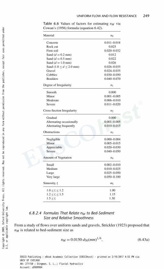
UNIFORM FLOW AND FLOW RESISTANCE 249
Table 6.6 Values of factors for estimating nM viaCowan’s (1956) formula (equation 6.42).
Material n0
Concrete 0.011–0.018Rock cut 0.025Firm soil 0.020–0.032Sand (d = 0.2 mm) 0.012Sand (d = 0.5 mm) 0.022Sand (d = 1.0 mm) 0.026Sand (1.0 ≤ d ≤ 2.0 mm) 0.026–0.035Gravel 0.024–0.035Cobbles 0.030–0.050Boulders 0.040–0.070
Degree of Irregularity n1
Smooth 0.000Minor 0.001–0.005Moderate 0.006–0.010Severe 0.011–0.020
Cross-Section Irregularity n2
Gradual 0.000Alternating occasionally 0.001–0.005Alternating frequently 0.010–0.015
Obstructions n3
Negligible 0.000–0.004Minor 0.005–0.015Appreciable 0.020–0.030Severe 0.040–0.050
Amount of Vegetation n4
Small 0.002–0.010Medium 0.010–0.025Large 0.025–0.050Very large 0.050–0.100
Sinuosity, � m�
1.0 ≤ � ≤ 1.2 1.001.2 ≤ � ≤ 1.5 1.151.5 ≤ � 1.30
6.8.2.4 Formulas That Relate nM to Bed-SedimentSize and Relative Smoothness
From a study of flows over uniform sands and gravels, Strickler (1923) proposed thatnM is related to bed-sediment size as
nM = 0.0150·d50(mm)1/6, (6.43a)
Copyright © 2009. Oxford University Press. All rights reserved. May not be reproduced in any form without permission from the publisher, except fair uses permitted under
U.S. or applicable copyright law.
EBSCO Publishing : eBook Academic Collection (EBSCOhost) - printed on 2/19/2017 4:55 PM viaUNIV OF CHICAGOAN: 271150 ; Dingman, S. L..; Fluvial HydraulicsAccount: s8989984
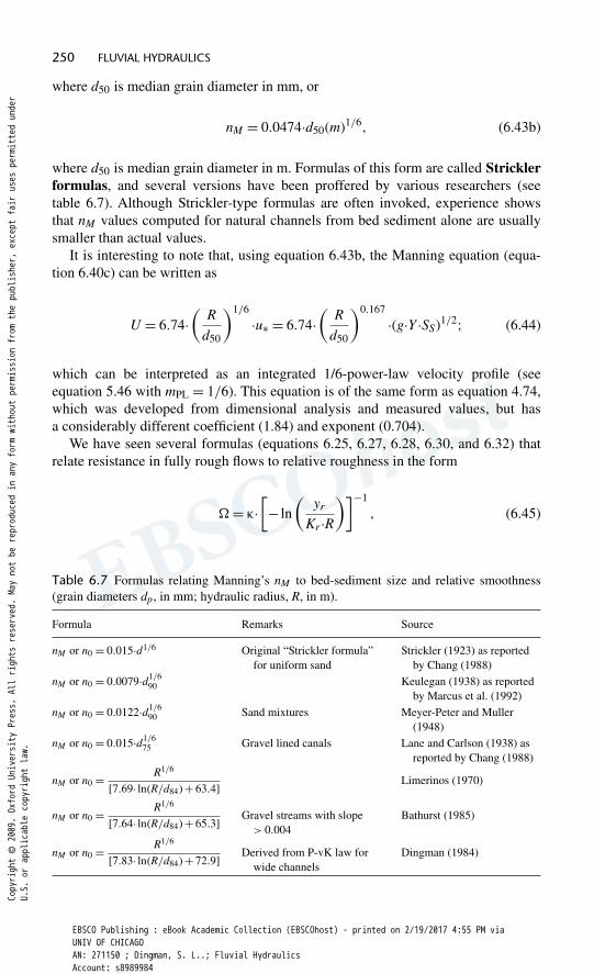
250 FLUVIAL HYDRAULICS
where d50 is median grain diameter in mm, or
nM = 0.0474·d50(m)1/6, (6.43b)
where d50 is median grain diameter in m. Formulas of this form are called Stricklerformulas, and several versions have been proffered by various researchers (seetable 6.7). Although Strickler-type formulas are often invoked, experience showsthat nM values computed for natural channels from bed sediment alone are usuallysmaller than actual values.
It is interesting to note that, using equation 6.43b, the Manning equation (equa-tion 6.40c) can be written as
U = 6.74·(
R
d50
)1/6
·u∗ = 6.74·(
R
d50
)0.167
·(g·Y ·SS)1/2; (6.44)
which can be interpreted as an integrated 1/6-power-law velocity profile (seeequation 5.46 with mPL = 1/6). This equation is of the same form as equation 4.74,which was developed from dimensional analysis and measured values, but hasa considerably different coefficient (1.84) and exponent (0.704).
We have seen several formulas (equations 6.25, 6.27, 6.28, 6.30, and 6.32) thatrelate resistance in fully rough flows to relative roughness in the form
� = �·[− ln
(yr
Kr ·R)]−1
, (6.45)
Table 6.7 Formulas relating Manning’s nM to bed-sediment size and relative smoothness(grain diameters dp, in mm; hydraulic radius, R, in m).
Formula Remarks Source
nM or n0 = 0.015·d1/6 Original “Strickler formula”for uniform sand
Strickler (1923) as reportedby Chang (1988)
nM or n0 = 0.0079·d1/690 Keulegan (1938) as reported
by Marcus et al. (1992)
nM or n0 = 0.0122·d1/690 Sand mixtures Meyer-Peter and Muller
(1948)
nM or n0 = 0.015·d1/675 Gravel lined canals Lane and Carlson (1938) as
reported by Chang (1988)
nM or n0 = R1/6
[7.69· ln(R/d84) + 63.4] Limerinos (1970)
nM or n0 = R1/6
[7.64· ln(R/d84) + 65.3] Gravel streams with slope> 0.004
Bathurst (1985)
nM or n0 = R1/6
[7.83· ln(R/d84) + 72.9] Derived from P-vK law forwide channels
Dingman (1984)
Copyright © 2009. Oxford University Press. All rights reserved. May not be reproduced in any form without permission from the publisher, except fair uses permitted under
U.S. or applicable copyright law.
EBSCO Publishing : eBook Academic Collection (EBSCOhost) - printed on 2/19/2017 4:55 PM viaUNIV OF CHICAGOAN: 271150 ; Dingman, S. L..; Fluvial HydraulicsAccount: s8989984

UNIFORM FLOW AND FLOW RESISTANCE 251
0.0000.0 0.5 1.0 1.5 2.0 2.5 3.0 3.5
0.010
0.020
0.030
0.040
0.050
0.060
0.070
R (m)
5 mm
R/d84 = 10
d
100 mm
50 mm
20 mm 10 mm
5 mm
2 mm
1 mm
n M
84 = 200 mm
Figure 6.23 Variation of Manning’s nM (or n0 in equation 6.42) with hydraulic radius, R,and bed grain diameter d84 as predicted by the Dingman (1984) version of equation 6.46 (seetable 6.7). Manning’s nM is effectively independent of depth for R/d84 > 10.
where the values of �, Kr , and yr take different values in different contexts. Ifequation 6.45 is substituted into equation 6.41, we find that
nM = uM ·�·R1/6
g1/2· ln(
Kr ·Ryr
) . (6.46)
Thus, equation 6.46 can be used to provide estimates of nM (or n0 in equation 6.42)in those contexts. Table 6.7 lists versions of equation 6.46 derived by various authors,and figure 6.23 shows the relation of nM to relative smoothness for various bed-sediment sizes in gravel-bed streams as given by the Dingman (1984) version ofthat equation. Note that the formula predicts little dependence of nM on R/d84 whenR/d84 > 10.
6.8.2.5 Statistically Derived Formulas That Relate nMto Hydraulic Variables
A number of researchers have used statistical analysis (regression analysis, asdescribed in section 4.8.3.1) to develop equations to predict nM based on measurableflow variables. Three of these equations are listed in table 6.8. There is considerableuncertainty associated with estimates from such equations: The equation of Dingmanand Sharma (1997), which is based on the most extensive data set, was found to give
Copyright © 2009. Oxford University Press. All rights reserved. May not be reproduced in any form without permission from the publisher, except fair uses permitted under
U.S. or applicable copyright law.
EBSCO Publishing : eBook Academic Collection (EBSCOhost) - printed on 2/19/2017 4:55 PM viaUNIV OF CHICAGOAN: 271150 ; Dingman, S. L..; Fluvial HydraulicsAccount: s8989984

252 FLUVIAL HYDRAULICS
Table 6.8 Statistically derived formulas for estimating Manning’s nM [A = cross-sectionalarea (m2); R = hydraulic radius (m); S =slope].
Formula Remarks Source
nM = 0.210·A−0.33·R0.667·S0.095 Based on 62 flows in Barnes (1967);0.024 ≤ nM ≤ 0.075
Riggs (1976)
nM = 0.32·R−0.16·S0.38 Mountain streams with 0.17 m ≤ R ≤ 2.13 mand 0.002 ≤ S ≤ 0.052
Jarrett (1984)
nM = 0.217·A−0.173·R0.267·S0.156 Based on 520 flows from Hicks and Mason(1991); 0.015 ≤ nM ≤ 0.290
Dingman andSharma (1997)
discharge estimates within ±50% of the true value 77% of the time. This topic isaddressed further in section 6.9.
6.8.2.6 Field Measurement of Discharge andHydraulic Variables
The only way that the value of Manning’s nM can be established with certaintyis by measuring the discharge and hydraulic variables at a given time in a givenreach, determining the prevailing reach-average velocity, and solving the Manningequation for nM . Ideally, one would repeat the calculations over a range of dischargesin a particular reach and use the nM values so determined in future a priori estimatesof velocity or discharge for that reach.
Barnes (1967) and Hicks and Mason (1991) give equations for direct computationof nM from measured values of discharge and surveyed values of cross-sectional area,hydraulic radius, reach length, and water-surface slope at several cross sections withina reach. However, their methodology is based on energy considerations (sections 4.5and 8.1), whereas the Manning equation is a modification of the Chézy equation,which was derived from momentum considerations (sections 4.4 and 8.2).9 Thus,it is preferable to compute resistance via the method described in section 6.7 forcomputing � (equation 6.39c); if desired, the corresponding nM value can then bedetermined via equation 6.41. In most cases, the two methods give very similar nM
values (within ±0.002).
6.8.3 Summary
As noted above, the Manning equation has been the most commonly used resistancerelation for most engineering and many scientific purposes. It is common to usethe expedient methods described in approaches 1–3 of table 6.3 to estimate nM inthese applications. However, it has been shown that even engineers with extensivefield experience generate a wide range of nM estimates for a given reach usingthese methods (Hydrologic Engineering Center 1986). Approach 4 is not usuallyappropriate for natural rivers because, as we have seen, resistance depends on manyfactors in addition to bed material. The various equations developed for approach5 can be used for conditions similar to those for which the particular equation wasestablished. Approach 6 can be useful, especially when trying to estimate discharge
Copyright © 2009. Oxford University Press. All rights reserved. May not be reproduced in any form without permission from the publisher, except fair uses permitted under
U.S. or applicable copyright law.
EBSCO Publishing : eBook Academic Collection (EBSCOhost) - printed on 2/19/2017 4:55 PM viaUNIV OF CHICAGOAN: 271150 ; Dingman, S. L..; Fluvial HydraulicsAccount: s8989984
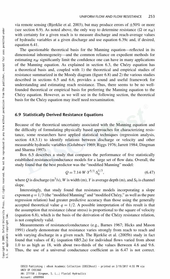
UNIFORM FLOW AND FLOW RESISTANCE 253
via remote sensing (Bjerklie et al. 2003), but may produce errors of ±50% or more(see section 6.9). As noted above, the only way to determine resistance (� or nM )with certainty for a given reach is to measure discharge and reach-average valuesof hydraulic variables at a given discharge and use equation 6.39c and, if desired,equation 6.41.
The questionable theoretical basis for the Manning equation—reflected in itsdimensional inhomogeneity—and the common reliance on expedient methods forestimating nM significantly limit the confidence one can have in many applicationsof the Manning equation. As explained in section 6.3, the Chézy equation hasa theoretical basis and, coupled with 1) the theoretical and empirical studies ofresistance summarized in the Moody diagram (figure 6.8) and 2) the various studiesdescribed in sections 6.5 and 6.6, provides a sound and useful framework forunderstanding and estimating reach resistance. Thus, there seems to be no well-founded theoretical or empirical basis for preferring the Manning equation to theChézy equation. However, as we will see in the following section, the theoreticalbasis for the Chézy equation may itself need reexamination.
6.9 Statistically Derived Resistance Equations
Because of the theoretical uncertainty associated with the Manning equation andthe difficulty of formulating physically based approaches for characterizing resis-tance, some researchers have applied statistical techniques (regression analysis,section 4.8.3.1) to identify relations between discharge or velocity and othermeasurable hydraulic variables (Golubtsev 1969; Riggs 1976; Jarrett 1984; Dingmanand Sharma 1997).
Box 6.5 describes a study that compares the performance of five statisticallyestablished resistance/conductance models for a large set of flow data. Overall, thestudy found that the best predictor was the “modified Manning” model:
Q = 7.14·W ·Y5/3·S1/30 , (6.47)
where Q is discharge (m3/s), W is width (m), Y is average depth (m), and S0 is channelslope.
Interestingly, that study found that resistance models incorporating a slopeexponent q = 1/3 (the “modified Manning” and “modified Chézy,” as well as the pureregression relation) had greater predictive accuracy than those using the generallyaccepted theoretical value q = 1/2. A possible interpretation of this result is thatthe assumption that resistance (shear stress) is proportional to the square of velocity(equation 6.8), which is the basis of the derivation of the Chézy resistance relation,is not completely valid.
Measurements of resistance/conductance (e.g., Barnes 1967; Hicks and Mason1991) clearly demonstrate that resistance varies strongly from reach to reach andwith varying discharge in a given reach. The Bjerklie et al. (2005b) study in factfound that values of K2 (equation 6B5.2a) for individual flows varied from about1.0 to as high as 18, with about two-thirds of the values Between 4.6 and 9.6.Thus, the use of a universal conductance coefficient as in 6.47 is not correct.
Copyright © 2009. Oxford University Press. All rights reserved. May not be reproduced in any form without permission from the publisher, except fair uses permitted under
U.S. or applicable copyright law.
EBSCO Publishing : eBook Academic Collection (EBSCOhost) - printed on 2/19/2017 4:55 PM viaUNIV OF CHICAGOAN: 271150 ; Dingman, S. L..; Fluvial HydraulicsAccount: s8989984
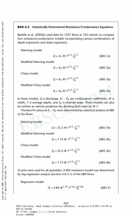
BOX 6.5 Statistically Determined Resistance/Conductance Equations
Bjerklie et al. (2005b) used data for 1037 flows at 103 reaches to comparefour resistance/conductance models incorporating various combinations ofdepth exponents and slope exponents.
Manning model:
Q = K1·W ·Y 5/3·S1/20 (6B5.1a)
Modified Manning model:
Q = K2·W ·Y 5/3·S1/30 (6B5.2a)
Chézy model:
Q = K3·W ·Y 3/2·S1/20 (6B5.3a)
Modified Chézy model
Q = K4·W ·Y 3/2·S1/30 (6B5.4a)
In these models, Q is discharge, K1 − K4 are conductance coefficients, W iswidth, Y is average depth, and S0 is channel slope. These models can alsobe written as velocity predictors by dividing both sides by W ·Y .
The best-fit values of K1 −K4 were determined by statistical analysis of 680of the flows.
Manning model:
Q = 23.3·W ·Y 2/3·S1/20 (6B5.1b)
Modified Manning model:
Q = 7.14·W ·Y 5/3·S1/30 (6B5.2b)
Chézy model:
Q = 25.2·W ·Y 3/2·S1/20 (6B5.3b)
Modified Chézy model:
Q = 7.73·W ·Y 3/2·S1/30 (6B5.4b)
SI units were used for all quantities. A fifth resistance model was determinedby log-regression analysis (section 4.8.3.1) of the 680 flows.
Regression model:
Q = 4.84·W1.10·Y 1.63·S0.3300 (6B5.5)
254
Copyright © 2009. Oxford University Press. All rights reserved. May not be reproduced in any form without permission from the publisher, except fair uses permitted under
U.S. or applicable copyright law.
EBSCO Publishing : eBook Academic Collection (EBSCOhost) - printed on 2/19/2017 4:55 PM viaUNIV OF CHICAGOAN: 271150 ; Dingman, S. L..; Fluvial HydraulicsAccount: s8989984
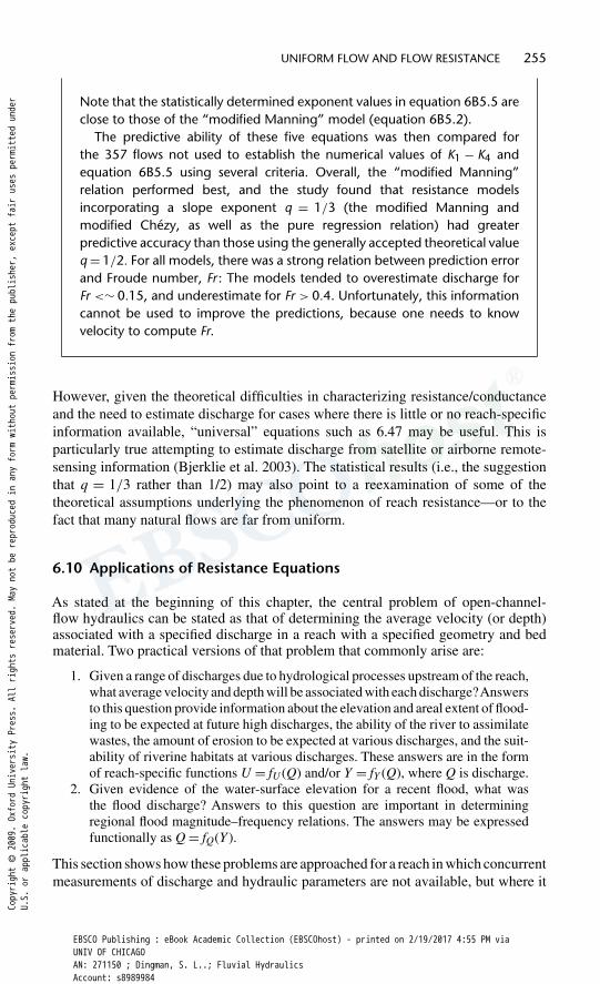
UNIFORM FLOW AND FLOW RESISTANCE 255
Note that the statistically determined exponent values in equation 6B5.5 areclose to those of the “modified Manning” model (equation 6B5.2).
The predictive ability of these five equations was then compared forthe 357 flows not used to establish the numerical values of K1 − K4 andequation 6B5.5 using several criteria. Overall, the “modified Manning”relation performed best, and the study found that resistance modelsincorporating a slope exponent q = 1/3 (the modified Manning andmodified Chézy, as well as the pure regression relation) had greaterpredictive accuracy than those using the generally accepted theoretical valueq = 1/2. For all models, there was a strong relation between prediction errorand Froude number, Fr : The models tended to overestimate discharge forFr <∼ 0.15, and underestimate for Fr > 0.4. Unfortunately, this informationcannot be used to improve the predictions, because one needs to knowvelocity to compute Fr.
However, given the theoretical difficulties in characterizing resistance/conductanceand the need to estimate discharge for cases where there is little or no reach-specificinformation available, “universal” equations such as 6.47 may be useful. This isparticularly true attempting to estimate discharge from satellite or airborne remote-sensing information (Bjerklie et al. 2003). The statistical results (i.e., the suggestionthat q = 1/3 rather than 1/2) may also point to a reexamination of some of thetheoretical assumptions underlying the phenomenon of reach resistance—or to thefact that many natural flows are far from uniform.
6.10 Applications of Resistance Equations
As stated at the beginning of this chapter, the central problem of open-channel-flow hydraulics can be stated as that of determining the average velocity (or depth)associated with a specified discharge in a reach with a specified geometry and bedmaterial. Two practical versions of that problem that commonly arise are:
1. Given a range of discharges due to hydrological processes upstream of the reach,what average velocity and depth will be associated with each discharge?Answersto this question provide information about the elevation and areal extent of flood-ing to be expected at future high discharges, the ability of the river to assimilatewastes, the amount of erosion to be expected at various discharges, and the suit-ability of riverine habitats at various discharges. These answers are in the formof reach-specific functions U = fU (Q) and/or Y = fY (Q), where Q is discharge.
2. Given evidence of the water-surface elevation for a recent flood, what wasthe flood discharge? Answers to this question are important in determiningregional flood magnitude–frequency relations. The answers may be expressedfunctionally as Q = fQ(Y ).
This section shows how these problems are approached for a reach in which concurrentmeasurements of discharge and hydraulic parameters are not available, but where it
Copyright © 2009. Oxford University Press. All rights reserved. May not be reproduced in any form without permission from the publisher, except fair uses permitted under
U.S. or applicable copyright law.
EBSCO Publishing : eBook Academic Collection (EBSCOhost) - printed on 2/19/2017 4:55 PM viaUNIV OF CHICAGOAN: 271150 ; Dingman, S. L..; Fluvial HydraulicsAccount: s8989984
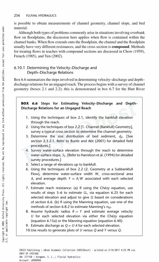
256 FLUVIAL HYDRAULICS
is possible to obtain measurements of channel geometry, channel slope, and bedmaterial.
Although both types of problems commonly arise in situations involving overbankflow on floodplains, the discussion here applies when flow is contained within thechannel banks. When flow extends onto the floodplain, the channel and the floodplainusually have very different resistances, and the cross section is compound. Methodsfor treating flows in reaches with compound sections are discussed in Chow (1959),French (1985), and Yen (2002).
6.10.1 Determining the Velocity–Discharge andDepth–Discharge Relations
Box 6.6 summarizes the steps involved in determining velocity–discharge and depth–discharge relations for an ungaged reach. The process begins with a survey of channelgeometry (boxes 2.1 and 2.2); this is demonstrated in box 6.7 for the Hutt River
BOX 6.6 Steps for Estimating Velocity–Discharge and Depth–Discharge Relations for an Ungaged Reach
1. Using the techniques of box 2.1, identify the bankfull elevationthrough the reach.
2. Using the techniques of box 2.2 [1. Channel (Bankfull) Geometry],survey a typical cross section to determine the channel geometry.
3. Determine the size distribution of bed sediment, dp. [Seesection 2.3.2.1. Refer to Bunte and Abt (2001) for detailed fieldprocedures.]
4. Survey water-surface elevation through the reach to determinewater-surface slope, SS . [Refer to Harrelson et al. (1994) for detailedsurvey procedures.]
5. Select a range of elevations up to bankfull.6. Using the techniques of box 2.2 (2. Geometry at a Subbankfull
Flow), determine water-surface width W , cross-sectional areaA, and average depth Y ≡ A/W associated with each selectedelevation.
7. Estimate reach resistance: (a) If using the Chézy equation, useresults of steps 3–6 to estimate �∗ via equation 6.25 for eachselected elevation and adjust to give � based on considerationsof section 6.6. (b) If using the Manning equation, use one of themethods of section 6.8.2 to estimate Manning’s nM .
8. Assume hydraulic radius R = Y and estimate average velocityU for each selected elevation via either the Chézy equation(equation 6.15a) or the Manning equation (equation 6.40).
9. Estimate discharge as Q = U·A for each selected elevation.10.Use results to generate plots of U versus Q and Y versus Q.
Copyright © 2009. Oxford University Press. All rights reserved. May not be reproduced in any form without permission from the publisher, except fair uses permitted under
U.S. or applicable copyright law.
EBSCO Publishing : eBook Academic Collection (EBSCOhost) - printed on 2/19/2017 4:55 PM viaUNIV OF CHICAGOAN: 271150 ; Dingman, S. L..; Fluvial HydraulicsAccount: s8989984

BOX 6.7 Example Computation of Channel Geometry: Hutt River atKaitoke, New Zealand
The line of a cross section is oriented at right angles to the general flowdirection. An arbitrary zero point is established at one end of the line; byconvention, this is usually on the left bank (facing downstream), but it canbe on either bank. Points are selected along the line to define the cross-section shape; these are typically “slope breaks”—points where the ground-surface slope changes. An arbitrary elevation datum is established, and theelevations of these points above this datum are determined by surveying(see Harrelson et al. 1994). To illustrate the computations, we use data fora cross section of the Hutt River in New Zealand (figure 6.24). Section surveyresults are recorded as elevations, zi , at distances along the section line, wi .At each point, the local bankfull depth YBFi can be calculated as
YBFi = �BF − zi , (6B7.1)
where �BF is the bankfull maximum depth. The data for the Hutt Riversection are given in table 6B7.1 and are plotted in figure 6.25.
Table 6B7.1
wi (m) 0.0 1.0 5.5 7.5 9.0 10.0 11.2 13.3 13.4 14.5zi (m) 3.78 3.71 2.72 2.18 1.92 1.50 0.96 0.86 0.85 0.54YBFi (m) 0.00 0.07 1.06 1.60 1.86 2.28 2.82 2.92 3.13 3.24
wi (m) 17.5 19.8 19.9 20.6 21.3 24.0 25.8 27.7 28.8 30.0zi (m) 0.53 0.58 0.32 0.28 0.41 0.30 0.44 0.12 0.00 0.24YBFi (m) 3.25 3.20 3.46 3.50 3.37 3.49 3.34 3.66 3.78 3.54
wi (m) 32.3 34.3 35.1 38.4 39.9 41.2 42.5 43.5 44.8 45.0zi (m) 0.23 0.29 0.50 0.64 0.80 1.84 2.41 2.90 3.71 3.78YBFi (m) 3.55 3.49 3.28 3.14 2.98 1.94 1.37 0.88 0.07 0.00
Once the section is plotted, several arbitrary elevations are identified torepresent water-surface elevations (the horizontal lines in figure 6.25). Foreach level, the horizontal positions of the left- and right-bank intersectionsof the level line with the channel bottom are determined and identifiedas wL and wR, respectively. For each selected elevation, the water-surfacewidth W is
W = |wR − wL|. (6B7.2)
Selecting the level � = 2 m in the Hutt River cross section for examplecalculations, we see from figure 6.25 that
W = |41.5 − 8.5| = 33.0 m.(Continued)
257
Copyright © 2009. Oxford University Press. All rights reserved. May not be reproduced in any form without permission from the publisher, except fair uses permitted under
U.S. or applicable copyright law.
EBSCO Publishing : eBook Academic Collection (EBSCOhost) - printed on 2/19/2017 4:55 PM viaUNIV OF CHICAGOAN: 271150 ; Dingman, S. L..; Fluvial HydraulicsAccount: s8989984

BOX 6.7 Continued
The cross-sectional area A associated with a given level is found as
A =N∑
i = 1
Ai =N∑
i = 1
Wi ·Yi , (6B7.3)
where Wi is the incremental width associated with each surveyed depth Yi , Nis the number of points for which we have observations, and i = 1,2, . . .,N. Ifwe start from the left bank, W1 = wL, WN = wR, and Y1 = 0, YN = 0 in all cases.The values of the incremental widths are determined as
W1 = |w2 − w1|2
; (6B7.4a)
Wi = |wi + 1 − wi − 1|2
, i = 2,3, . . .,N −1; (6B7.4b)
WN = |wN − wN − 1|2
. (6B7.6c)
Note that �Wi = W .Table 6B7.2 gives the data for the � = 2 m elevation in the Hutt River cross
section.
Table 6B7.2
i wi (m) Yi (m) Wi (m) Ai (m2)
1 8.5 0.00 0.25 0.0002 9.0 0.08 0.75 0.0633 10.0 0.50 1.10 0.5534 11.2 1.04 1.65 1.7215 13.3 1.14 1.10 1.2536 13.4 1.35 0.60 0.8097 14.5 1.46 2.05 2.9998 17.5 1.47 2.65 3.9039 19.8 1.42 1.20 1.708
10 19.9 1.68 0.40 0.67111 20.6 1.72 0.70 1.20612 21.3 1.59 1.70 2.70113 24.0 1.71 2.25 3.83614 25.8 1.56 1.85 2.88215 27.7 1.88 1.50 2.81716 28.8 2.00 1.15 2.30017 30.0 1.76 1.75 3.08018 32.3 1.77 2.15 3.81219 34.3 1.71 1.40 2.39520 35.1 1.50 2.05 3.07321 38.4 1.36 2.40 3.25722 39.9 1.20 1.40 1.68023 41.2 0.16 0.80 0.13024 41.5 0.00 0.15 0.000Sum 33.00 = W 46.851 = A
258
Copyright © 2009. Oxford University Press. All rights reserved. May not be reproduced in any form without permission from the publisher, except fair uses permitted under
U.S. or applicable copyright law.
EBSCO Publishing : eBook Academic Collection (EBSCOhost) - printed on 2/19/2017 4:55 PM viaUNIV OF CHICAGOAN: 271150 ; Dingman, S. L..; Fluvial HydraulicsAccount: s8989984
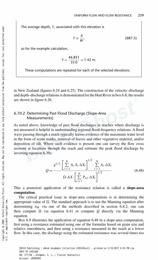
UNIFORM FLOW AND FLOW RESISTANCE 259
The average depth, Y , associated with this elevation is
Y ≡ AW
, (6B7.5)
so for the example calculation,
Y = 46.85133.0
= 1.42 m.
These computations are repeated for each of the selected elevations.
in New Zealand (figures 6.24 and 6.25). The construction of the velocity–dischargeand depth–discharge relations is demonstrated for the Hutt River in box 6.8; the resultsare shown in figure 6.26.
6.10.2 Determining Past Flood Discharge (Slope-AreaMeasurements)
As noted above, knowledge of past flood discharges in reaches where discharge isnot measured is helpful in understanding regional flood-frequency relations. A floodwave passing through a reach typically leaves evidence of the maximum water levelin the form of scour marks, removal of leaves and other vegetative material, and/ordeposition of silt. Where such evidence is present one can survey the flow crosssections at locations through the reach and estimate the peak flood discharge byinverting equation 6.39c:
Q =g1/2·
[N∑
i = 1Ai·Si·�Xi
]1/2
·N∑
i = 1Ai·�Xi
�·�X·[
N∑i = 1
Pwi·�Xi
]1/2(6.48)
This a posteriori application of the resistance relation is called a slope-areacomputation.
The critical practical issue in slope-area computations is in determining theappropriate value of �. The standard approach is to use the Manning equation afterdetermining nM via one of the methods described in section 6.8.2; one canthen compute � via equation 6.41 or compute Q directly via the Manningequation.
Box 6.9 illustrates the application of equation 6.48 in a slope-area computation,first using a resistance estimated using one of the formulas based on grain size andrelative smoothness, and then using a resistance measured in the reach at a lowerflow. In this case, the discharge using the estimated resistance was several times too
Copyright © 2009. Oxford University Press. All rights reserved. May not be reproduced in any form without permission from the publisher, except fair uses permitted under
U.S. or applicable copyright law.
EBSCO Publishing : eBook Academic Collection (EBSCOhost) - printed on 2/19/2017 4:55 PM viaUNIV OF CHICAGOAN: 271150 ; Dingman, S. L..; Fluvial HydraulicsAccount: s8989984

260 FLUVIAL HYDRAULICS
Figure 6.24 The Hutt River at Kaitoke, New Zealand. (a) View downstream at middle ofreach. (b) View upstream at middle of reach. From Hicks and Mason (1991); reproduced withpermission of New Zealand National Institute of Water and Atmospheric Research Ltd.
large (i.e., resistance was severely underestimated), while the discharge using themeasured resistance was within 2% of the actual value. However, such good resultsmay not always be obtained even with resistance values measured in the reach ofinterest, because one or more of the factors discussed in section 6.6 may have beensignificantly different at the time of the peak flow than at the time of measurement(Kirby 1987):
Cross-section geometry: The peak flow may have scoured the channel bed andsubsequent lower flows deposited bed sediment. If this happened, the cross-sectional area that existed at the time of the peak flow was larger than the surveyedvalues and the peak discharge will be underestimated.
Plan-view irregularity: In meandering streams, high flows may “short-circuit” thebends, leading to lower resistance at the high flow than when measured at lowerflows.
Copyright © 2009. Oxford University Press. All rights reserved. May not be reproduced in any form without permission from the publisher, except fair uses permitted under
U.S. or applicable copyright law.
EBSCO Publishing : eBook Academic Collection (EBSCOhost) - printed on 2/19/2017 4:55 PM viaUNIV OF CHICAGOAN: 271150 ; Dingman, S. L..; Fluvial HydraulicsAccount: s8989984

0.00 5 10 15 20 25 30 35 40 45 50
0.5
1.0
1.5
2.0
2.5
3.0
3.5
4.0
Distance from Left Bank (m)
Elev
atio
n (m
)
ψ = 0.50 m
ψ = 1.00 m
ψ = 1.50 m
ψ = 2.00 m
ψ = 2.50 m
ψ = 3.00 m
ψBF = 3.78 m
ψ = 3.50 m
Figure 6.25 Surveyed cross section in the center of the Hutt River reach shown in figure 6.24.Elevations are relative to the lowest elevation in the cross section. The dashed lines are thewater levels at the maximum depths (�) indicated; �BF is the bankfull maximum depth. Noteapproximately 10-fold vertical exaggeration.
BOX 6.8 Example Computation of Velocity–Discharge and Depth–Discharge Relations for an Ungaged Reach: Hutt River at Kaitoke,New Zealand
Using the procedure described in boxes 6.6 and 6.7, the following values ofaverage depth Y have been computed for selected maximum-depth levels �
for the cross section of the Hutt River at Kaitoke, New Zealand, shown infigure 6.25:
Ψ (m) 0.50 1.00 1.50 2.00 2.50 3.00 3.50 3.78Y (m) 0.22 0.55 1.01 1.42 1.77 2.11 2.44 2.57
The bed-sediment material consists of gravel, cobbles, and boulders; d84 =212 mm. The average channel slope through the reach is S = 0.00539. Weestimate the velocity–discharge and depth–discharge relations for this crosssection via 1) the Chézy equation and 2) the Manning equation.
Chézy Equation
There is a range of bed-material sizes; we select the resistance relationfor gravel-bed streams suggested by Bathurst (1993) (equation 6.27).
(Continued)
Copyright © 2009. Oxford University Press. All rights reserved. May not be reproduced in any form without permission from the publisher, except fair uses permitted under
U.S. or applicable copyright law.
EBSCO Publishing : eBook Academic Collection (EBSCOhost) - printed on 2/19/2017 4:55 PM viaUNIV OF CHICAGOAN: 271150 ; Dingman, S. L..; Fluvial HydraulicsAccount: s8989984

BOX 6.8 Continued
We assume R = Y and estimate � as
� = 0.400·[− ln
(0.2123.60·R
)]−1.
Values of u∗ are determined via equation 6.16:
u∗ = (9.81·R·0.00539)1/2
Average velocity U is then computed via equation 6.19 and discharge Q viaequation 6.3. The results are tabulated in table 6B8.1.
Table 6B8.1
� (m) 0.50 1.00 1.50 2.00 2.50 3.00 3.50 3.78R (m) 0.22 0.55 1.01 1.42 1.77 2.11 2.44 2.57� 0.301 0.179 0.141 0.126 0.118 0.112 0.107 0.106U (m/s) 0.359 0.956 1.642 2.180 2.603 2.988 3.344 3.480Q (m3/s) 1.19 15.3 50.9 102 167 249 348 404
Manning Equation
In practice, one would use one of the approaches listed in table 6.3 anddiscussed in section 6.8.2 to estimate the appropriate nM for this reach. Inthis example, we will use the value determined for the reach by measurementand reported in Hicks and Mason (1991): nM = 0.037. Using this value andthe measured slope in the Manning equation (equation 6.40c), we computethe values in table 6B8.2.
Table 6B8.2
� (m) 0.50 1.00 1.50 2.00 2.50 3.00 3.50 3.78R (m) 0.22 0.55 1.01 1.42 1.77 2.11 2.44 2.57U (m/s) 0.727 1.335 2.000 2.507 2.903 3.264 3.596 3.723Q (m3/s) 2.42 21.4 61.9 118 187 272 374 432
Comparison of Estimates with Measured Values
Hicks and Mason (1991) provided measured values of R, U, and Q for thisreach, so we can compare the two estimates with actual values, as shown infigure 6.26. The Chézy estimate, which uses only measured quantities (R, S,d84) fits the measured values very closely except at the highest flow, whilethe Manning estimate of velocity is slightly too high (and depth too low)over most of the range. Recall though that the Manning estimate is basedon a value of nM determined by measurement in the reach; in many actualapplications, such measurements would not be available, and we would beforced to estimate nM by other means (section 6.8.2), probably leading togreater error.
In this example, the Chézy relation appears to give better results than theManning relation.
262
Copyright © 2009. Oxford University Press. All rights reserved. May not be reproduced in any form without permission from the publisher, except fair uses permitted under
U.S. or applicable copyright law.
EBSCO Publishing : eBook Academic Collection (EBSCOhost) - printed on 2/19/2017 4:55 PM viaUNIV OF CHICAGOAN: 271150 ; Dingman, S. L..; Fluvial HydraulicsAccount: s8989984
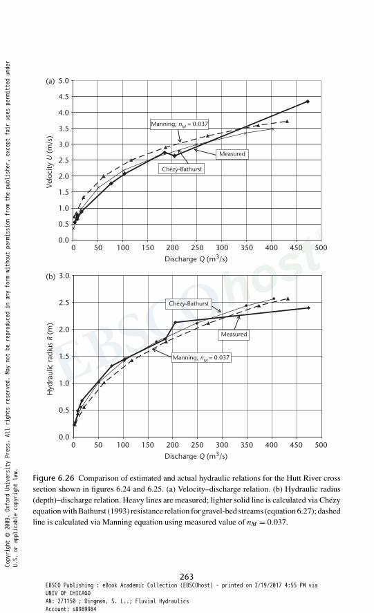
0.00 50 100 150 200 250 300 350 400 450 500
0.5
1.0
1.5
2.0
2.5
3.0
3.5
4.0
4.5
(a)
(b)
5.0
Discharge Q (m3/s)
0 50 100 150 200 250 300 350 400 450 500
Discharge Q (m3/s)
Velo
city
U (
m/s
)
Manning; nM = 0.037
Chézy-Bathurst
Measured
0.0
0.5
1.0
1.5
2.0
2.5
3.0
Hyd
raul
ic r
adiu
s R
(m)
Manning; nM = 0.037
Chézy-Bathurst
Measured
Figure 6.26 Comparison of estimated and actual hydraulic relations for the Hutt River crosssection shown in figures 6.24 and 6.25. (a) Velocity–discharge relation. (b) Hydraulic radius(depth)–discharge relation. Heavy lines are measured; lighter solid line is calculated via Chézyequation with Bathurst (1993) resistance relation for gravel-bed streams (equation 6.27); dashedline is calculated via Manning equation using measured value of nM = 0.037.
263
Copyright © 2009. Oxford University Press. All rights reserved. May not be reproduced in any form without permission from the publisher, except fair uses permitted under
U.S. or applicable copyright law.
EBSCO Publishing : eBook Academic Collection (EBSCOhost) - printed on 2/19/2017 4:55 PM viaUNIV OF CHICAGOAN: 271150 ; Dingman, S. L..; Fluvial HydraulicsAccount: s8989984

BOX 6.9 Slope-Area Computations, South Beaverdam Creek NearDewy Rose, Georgia
A peak flood on 26 November 1957 left high water marks in a reach of SouthBeaverdam Creek near Dewy Rose, Georgia. The peak flood discharge wasmeasured at Q = 23.2 m3/s. The cross-sectional area, width, average depth,hydraulic radius, wetted perimeter, and water-surface slope defined by thesehigh-water marks were surveyed by Barnes (1967) at five cross sections andare summarized in table 6B9.1.
Table 6B9.1
Section, i Ai (m2) Wi (m) Yi (m) Ri (m) Pwi (m) �Xi (m) �Zi (m) SSi = |�Zi |/�Xi
0 24.9 21.6 1.16 1.10 22.61 26.8 17.1 1.55 1.52 17.7 21.6 0.043 0.001972 25.8 18.0 1.43 1.32 19.5 20.1 0.037 0.001823 26.1 18.0 1.46 1.34 19.4 24.7 0.040 0.001614 24.2 17.7 1.37 1.26 19.2 19.5 0.018 0.00094
Averageor sum
A =25.6
W =18.5
Y =1.40
R =1.31
Pw =19.7
�X =85.9
�Z =0.137
SS = 0.00160
To illustrate slope-area computations, we assume the discharge is unknownand apply three approaches that could be used to estimate a past flooddischarge from high-water marks.
Standard Approach
This is the method described in section 6.8.2. We first assume we do nothave a resistance determined by measurement in the reach. Table 6B9.2gives the values of the quantities that are summed in equation 6.39c.
Table 6B9.2
Section, i Ai ·SSi ·�Xi (m3) Ai ·�Xi (m3) Pwi ·�Xi (m3)
1 1.143 579 3822 0.945 520 3933 1.035 645 4804 0.442 472 375Sum 3.465 2216 1630
The channel bed “consists of sand about 1 ft deep over clay and rock. Banksare irregular with trees and bushes growing down to the low water line”Barnes (1967, p. 142). Because this is a sand-bed reach, we estimate � viaequation 6.25 assuming Y = R and yr = d84 = 0.002 m (the upper limit forsand), and compute
� = 0.400·[− ln
(0.002
11·1.31
)]−1= 0.045.
264
Copyright © 2009. Oxford University Press. All rights reserved. May not be reproduced in any form without permission from the publisher, except fair uses permitted under
U.S. or applicable copyright law.
EBSCO Publishing : eBook Academic Collection (EBSCOhost) - printed on 2/19/2017 4:55 PM viaUNIV OF CHICAGOAN: 271150 ; Dingman, S. L..; Fluvial HydraulicsAccount: s8989984

Substituting the appropriate values into equation 6.48 gives
Q = 9.811/2· [3.465]1/2 ·2216
0.045·85.9· [1630]1/2 = 82.8 m3/s
as our estimate of peak discharge.This estimate is several times too high. Thus, it appears that we severely
underestimated the resistance using equation 6.25. Some of the “excess”resistance probably comes from the bank vegetation that extended into theflow, and some may be due to the development of ripples or dunes on the sandbed. Perhaps we could have come up with a better estimate using another ofthe approaches of section 6.8.2, or had accounted for effects of bedforms onthe resistance (see section 6.6.4.2).
A better approach would be to determine the reach resistance viameasurement before applying equation 6.48. On the day after the 26November flood, when the flow was Q = 6.26 m3/s, Barnes (1967) surveyedthe same cross sections and obtained the values in table 6B9.3.
Table 6B9.3
Section, i Ai (m2) Ri (m) Pwi (m) �Xi (m) |�Zi |(m) SSi = |�Zi |/�Xi
0 8.5 0.62 13.71 11.9 0.82 14.5 21.6 0.034 0.001552 10.0 0.61 16.5 20.1 0.030 0.001523 10.0 0.60 16.6 24.7 0.024 0.000994 9.4 0.62 15.1 19.5 0.043 0.00219Averageor sum
A = 9.96 R = 0.65 Pw = 15.3 �X = 85.9 |�Z| = 0.131 SS = 0.00153
We want to determine the value of � for this flow and use that value to estimatethe flood peak on 26 November 1957. Table 6B9.4 gives the values of thequantities that are summed in equation 6.39c.
Table 6B9.4
Section, i Ai ·SSi ·�Xi (m3) Ai ·�Xi (m3) Pwi ·�Xi (m3)
1 0.399 258 3142 0.306 202 3313 0.245 248 4114 0.401 183 295
Sum 1.351 891 1351
Substituting the appropriate values into equation 6.39c yields
� = 9.811/2· [1.351]1/2 ·891
6.26·85.9· [1351]1/2 = 0.164.
(Continued)
265
Copyright © 2009. Oxford University Press. All rights reserved. May not be reproduced in any form without permission from the publisher, except fair uses permitted under
U.S. or applicable copyright law.
EBSCO Publishing : eBook Academic Collection (EBSCOhost) - printed on 2/19/2017 4:55 PM viaUNIV OF CHICAGOAN: 271150 ; Dingman, S. L..; Fluvial HydraulicsAccount: s8989984

BOX 6.9 Continued
Thus, the measured reach resistance is several times higher than that basedon equation 6.25. Finally, we use this measured value of � to estimate thepeak discharge of 26 November 1957 via equation 6.48:
Q = 9.811/2· [3.465]1/2 ·2216
0.164·85.9· [1630]1/2 = 22.7 m3/s
The value of Q estimated using the � value measured in the reach is within2% of the actual value.
Application of General Statistically Derived Relation
It is of interest to see how well the statistically developed “modifiedManning” equation (equation 6.47) does in estimating the peak flooddischarge from the high-water marks. Using values from table 6B9.1, thatequation gives
Q = 7.14·18.5·1.405/3·0.001601/3 = 27.1 m3/s.
The estimate for this case is quite good, about 17% higher than actual. TheFroude number for this flow can be calculated from data in table 6B9.1:
Fr = U(g·Y )1/2 = Q/A
(g·Y )1/2 = 23.2/25.6(9.81·1.40)1/2 = 0.24
This value is in the range where equation 6.47 was found to give generallygood predictions.
Application of Relation Developed from Dimensional Analysis
It is also of interest to see how well equation 4.74, developed by dimensionalanalysis and measurement data from New Zealand rivers, does in predictingthe flood-peak discharge. Recall that that relation, written in terms ofdischarge, is
Q = 1.84·(
Yyr
)0.704·g1/2·W ·Y 3/2·S1/2
0 ,Y/yr ≤ 10; (6B9.1a)
Q = 9.51·g1/2·W ·Y 3/2·S1/20 ,Y/yr > 10. (6B9.1b)
Since yr = 0.002 m, Y/yr > 10, and we use equation 6B9.1b with data fromtable 6B9.1:
Q = 9.51·9.811/2·18.5·1.403/2·0.001601/2 = 36.5 m3/s
This estimate is 57% greater than actual, suggesting that equation 4.74 isnot sufficiently precise to use for prediction (note the scatter in figure 4.14).
266
Copyright © 2009. Oxford University Press. All rights reserved. May not be reproduced in any form without permission from the publisher, except fair uses permitted under
U.S. or applicable copyright law.
EBSCO Publishing : eBook Academic Collection (EBSCOhost) - printed on 2/19/2017 4:55 PM viaUNIV OF CHICAGOAN: 271150 ; Dingman, S. L..; Fluvial HydraulicsAccount: s8989984

UNIFORM FLOW AND FLOW RESISTANCE 267
Longitudinal-profile irregularity: At high flows, the pool/riffle alteration tends tobecome submerged, tending to decrease resistance at higher flows (figure 6.11c).
Vegetation: Resistance may decrease at higher flows because flexible vegetationis bent further or because low vegetation becomes more submerged, or increasebecause more of the flow encounters bank and floodplain vegetation.
Surface stability: Resistance may increase at higher flows due to surfaceirregularities, particularly at bends or abrupt obstructions.
Sediment: In sand-bed streams, bedforms may be different at high flows than whenflow is measured, leading to higher or lower resistance (figure 6.20).
Ice: During breakup of an ice cover, there may be large and unknown differencesin resistance between the time of a high flow and when reach resistance ismeasured.
6.11 Summary
The standard approach to open-channel flow resistance is usually presented in termsof the Manning equation, with focus on determining appropriate values of Manning’snM in various applications. However, the Manning equation was not derived from firstprinciples, nor was it established by rigorous statistical analysis. Thus, this chapter hasexplored the fundamentals and practical aspects of resistance via the Chézy equation,which is derived from straightforward macroscopic force-balance considerations.This approach is consistent with fundamental fluid-mechanics principles:
• The Chézy derivation incorporates assumptions consistent with the models ofturbulence presented in section 3.3.4 .
• Formulating the resistance as the dimensionless quantity � allows us to considerthe subject in a way that is consistent with theoretical and observationalapproaches that are applicable in a wide range of fluid-mechanics contexts(summarized by the Moody diagram, figure 6.8).
• At least for the simplest flow situations, resistance can be related to measurablevariables via physically based expressions for the velocity profile discussed inchapter 5 (equation 6.25).
As noted at the beginning of this chapter, our goal has been to develop relationsfor computing the average velocity U in a channel reach given the reach geometry,material, and slope and the depth or discharge. We expressed this relation as
U = �−1·u∗ = �−1·(g·R·S)1/2 ≈ �−1·(g·Y ·S)1/2 (6.49)
and explored the factors that control �. Following Rouse (1965) and Yen (2002), wecan summarize these factors for quasi-uniform flows in natural channels:
� = f�(Y/yr,Re,Y/W ,�,ζ,�,V,Fr,�,I), (6.50a)
where � represents the effects of cross-section irregularities, ζ the effects ofplanform irregularities, � the effects of longitudinal-profile irregularities, V theeffects of vegetation, � the effects of sediment transport, and I the effects of ice.
Copyright © 2009. Oxford University Press. All rights reserved. May not be reproduced in any form without permission from the publisher, except fair uses permitted under
U.S. or applicable copyright law.
EBSCO Publishing : eBook Academic Collection (EBSCOhost) - printed on 2/19/2017 4:55 PM viaUNIV OF CHICAGOAN: 271150 ; Dingman, S. L..; Fluvial HydraulicsAccount: s8989984

268 FLUVIAL HYDRAULICS
Considering only ice-free channels and noting that the effects of Y/W are generallyminor in natural channels (figure 6.10), we can write
� ≈ f�(Y/yr,Re,�,ζ,�,V,Fr,�). (6.50b)
Further simplification may be possible if we recall that the effects of cross-sectionalvariability � and longitudinal variability � are at least in part captured by the relativesubmergence Y/yr , so that
� ≈ f�(Y/yr,Re,ζ,V,Fr,�). (6.50c)
One barrier to using 6.50c to determine velocity via 6.49 is that Re, ζ, Fr, �, andto some extent V all depend on velocity—so we are faced with a logical circularity.However, if we confine ourselves to fully rough flows in wide, reasonably straightchannels at low to moderate Froude numbers and insignificant sediment transport,the problem becomes more tractable:
� ≈ f�(Y/yr). (6.50d)
Based on the P-vK law and the analyses in section 6.6, we can be reasonably confidentthat the form of this relation is given by
� ≈ �·[
ln
(Kr ·Y
yr
)]−1
. (6.51)
The standard form of this relation is the C-K equation, in which �= 0.400 and Kr = 11.However, as we have seen in equations 6.27, 6.28, 6.30, and 6.32, the values of � andKr may vary from reach to reach—and maybe even for different flows in the samereach.
We saw in box 6.7 that the Chézy approach incorporating an appropriate resistancerelation can provide good estimates of velocity-discharge and depth-dischargerelations that can be used to solve practical problems.
Approaching resistance via the Chézy equation also provides a straightforwardformula for computing reach resistance from field data (equation 6.39). This formulacan be inverted to give a relation for estimating past flood discharges in slope-areacomputations (equation 6.48). However, we saw in box 6.9 that such estimates canbe erroneous in the absence of appropriate resistance estimates.
Clearly, although we have learned much about the factors that determine reachresistance, there are still many uncertainties to be faced in obtaining reliable a prioriand a posteriori resistance estimates for practical use and much need for additionalresearch in this area.
Copyright © 2009. Oxford University Press. All rights reserved. May not be reproduced in any form without permission from the publisher, except fair uses permitted under
U.S. or applicable copyright law.
EBSCO Publishing : eBook Academic Collection (EBSCOhost) - printed on 2/19/2017 4:55 PM viaUNIV OF CHICAGOAN: 271150 ; Dingman, S. L..; Fluvial HydraulicsAccount: s8989984

7
Forces and Flow Classification
7.0 Introduction and Overview
The forces involved in open-channel flow are introduced in section 4.2.2.1. Thegoals of this chapter are 1) to develop expressions to evaluate the magnitudes ofthose forces at the macroscopic scale, 2) to examine the relative magnitudes of thevarious forces in natural channels and show how they change with the flow scale, and3) to show that the Reynolds number (introduced in section 3.4.2) and the Froudenumber (introduced in section 6.2.2.2) can be interpreted in terms of force ratios.Understanding the relative magnitudes of forces provides a helpful perspective fordeveloping quantitative solutions to practical problems.
Open-channel flows are induced by gradients of potential energy proportional to thesine of the water-surface slope (section 4.7). This chapter shows that the water-surfaceslope reflects the magnitude of the driving forces due to gravity and pressure. Oncemotion begins, frictional forces resisting the flow arise due to molecular viscosity and,usually, turbulence; these forces are increasing functions of velocity. In steady uniformflow, which was assumed in the developments of chapters 5 and 6, the gravitationaldriving force is balanced by the frictional forces, so there is no acceleration and noother forces are involved. However, in general, the forces affecting open-channelflows are not in balance, so the flow experiences convective acceleration (spatialchange in velocity) and/or local acceleration (temporal change in velocity)—conceptsintroduced in section 4.2.1.2 at the “microscopic” scale (fluid elements).
In this chapter, as in chapters 5 and 6, we continue to analyze the flow on amacroscopic scale; that is, the physical relations are developed for the entire flow ina reach in an idealized channel rather than for a fluid element. We consider changesonly in time and in one spatial dimension (the downstream direction), so the resultingequations are characterized as “one-dimensional.”
269
Copyright © 2009. Oxford University Press. All rights reserved. May not be reproduced in any form without permission from the publisher, except fair uses permitted under
U.S. or applicable copyright law.
EBSCO Publishing : eBook Academic Collection (EBSCOhost) - printed on 2/19/2017 4:55 PM viaUNIV OF CHICAGOAN: 271150 ; Dingman, S. L..; Fluvial HydraulicsAccount: s8989984

270 FLUVIAL HYDRAULICS
The chapter begins by reviewing the forces that induce and oppose fluid motionin open channels and presenting the basic force-balance equations for various flowcategories. Next we lay out the basic geometry of an idealized reach and then formulatequantitative expressions for the magnitudes of the various forces as functions of fluidproperties and flow parameters. We also develop expressions for the convective andlocal accelerations so that we can ultimately formulate the complete macroscopicforce-balance equation for one-dimensional open-channel flow.
Using data for a range of flows, we examine the typical values of each of theforces in natural streams and compare their magnitudes. We also compare the relativemagnitudes of the forces as a function of scale, from small laboratory flumes to theGulf Stream. This comparison provides guidance for identifying conditions underwhich the force balance may be simplified by omitting particular forces due to theirrelative insignificance. The chapter concludes by showing how the Reynolds andFroude numbers can be interpreted in terms of force ratios.
7.1 Force Classification and the Overall Force Balance
In this section we formulate the overall force-balance relations for flows of variouscategories. To simplify the development, these relations are formulated for the simpleopen-channel flow shown in figure 7.1: a wide rectangular channel (Y = R) withconstant width (W1 = W2 = W ) but spatially varying depth. At any instant, the reachcontains a spatially constant discharge Q, so
Q = W · Y1 · U1 = W · Y2 · U2, (7.1)
where Yi is the average depth and Ui is the average velocity at section i.
Y1
Y2
U1
U2
Z1
Z2
θS
ΔX
θ0
Datum
Figure 7.1 Definition diagram for deriving expressions to calculate force magnitudes for anonuniform flow in a prismatic channel. Width and discharge are assumed constant.
Copyright © 2009. Oxford University Press. All rights reserved. May not be reproduced in any form without permission from the publisher, except fair uses permitted under
U.S. or applicable copyright law.
EBSCO Publishing : eBook Academic Collection (EBSCOhost) - printed on 2/19/2017 4:55 PM viaUNIV OF CHICAGOAN: 271150 ; Dingman, S. L..; Fluvial HydraulicsAccount: s8989984