Understanding Equity Option Prices�

Peter Christo¤ersen Mathieu Fournier Kris Jacobs

University of Toronto University of Toronto University of Houston

CBS and CREATES and Tilburg University

April 13, 2012

Abstract

Principal component analysis of equity options on Dow-Jones �rms reveals a strong factor

structure. The �rst principal component explains 66% of the variation in equity volatility

level, 65% of the variation in the equity option skew and 61% of the implied volatility term

structure across equities. Furthermore, the �rst principal component has an 88% correlation

with S&P500 index option volatility, an 83% correlation with the index option skew, and a 66%

correlation with the index option term structure. Based on these �ndings we develop an equity

option valuation model that captures the cross-sectional market factor structure as well as sto-

chastic volatility through time. The model assumes a Heston (1993) style stochastic volatility

model for the market return but additionally allows for stochastic idiosyncratic volatility for

each �rm. The model delivers theoretical predictions consistent with the empirical �ndings in

Duan and Wei (2009). We provide a tractable approach for estimating the model on index

and equity option data. The model provides a good �t to a large panel of options on stocks in

the Dow-Jones index.

JEL Classi�cation: G10; G12; G13.

Keywords: Factor models; equity options; implied volatility; option-implied beta.

�We are grateful to Redouane Elkamhi, Jason Wei, and Alan White for helpful discussion and to SSHRC for�nancial support. Contact: Peter Christo¤ersen, Rotman School of Management, 105 St. George Street Toronto,Ontario, Canada M5S 3E6. E-mail: peter.christo¤ersen@rotman.utoronto.ca.

1

1 Introduction

While factor models are standard for understanding equity prices, classic equity option valuation

models make no attempt at modeling a factor structure in the underlying equity prices.1 Typically,

a stochastic process is assumed for each underlying equity price and the option is priced on this

stochastic process ignoring any links the underlying equity price may have with other equity prices

through common factors.

When considering a single stock option, ignoring an underlying equity factor structure may be

relatively harmless. However, in portfolio applications it is crucial to understand links between the

underlying stocks: Risk managers need to understand the total exposure to the underlying risk

factors in a portfolio of stocks and stock options. Equity portfolio managers who use equity options

to hedge large downside moves in individual stocks need to know their overall market exposure.

Dispersion traders who sell (expensive) index options and buy (cheaper) equity options to hedge

need to understand the market exposure of individual equity options.2

Our empirical analysis of over two hundred thousand index options and close to one million

equity option contracts reveals a very strong factor structure. We study three aspects of option

prices: short-term implied volatility (IV) levels, the slope of IV curves across option moneyness,

and the slope of IV curves across option maturity.

First, we construct daily time series of short-term at-the-money implied volatility (IV) on the

stocks in the Dow Jones Industrials Average and extract their principal components. The �rst

common component explains roughly 66% of the cross-sectional variation in IV and the common

component has an 88% correlation with the short-term implied volatility constructed from S&P500

index options. Short term equity option IV appears to have a very strong common market factor.

Second, a principal component analysis of equity option IV across moneyness (the option �skew�)

reveals a surprisingly strong common component as well. Roughly 65% of the variation in the skew

across equities is captured by the �rst principal component. Furthermore, this common component

has a correlation of 83% with the skew of market index options.

Third, when looking for a common component in the term structure of equity IV we �nd that

61% of the variation is explained by the �rst principal component. This component has a correlation

of 66% with the term slope of the option IV from S&P500 index options.

We use the �ndings from the principal component analysis to develop a structural model of

equity option prices that incorporates a market factor structure. In line with well-known empirical

1Notable examples include Black and Scholes (1973), Wiggins (1987), Hull and White (1987), Heston (1993) andmany others.

2See Driessen, Maenhout and Vilkov (2009).

2

facts in the literature on index options,3 our model allows for mean-reverting stochastic volatility

and correlated shocks to return and volatility. Motivated by our principal component analysis, we

allow for idiosyncratic shocks to equity prices which also have mean-reverting stochastic volatility

and a separate leverage e¤ect. Individual equity returns are linked to the market index using a

standard linear factor model with a constant �beta�factor loading. Our model belongs to the a¢ ne

class which enables us to derive closed-form option pricing formulas. The model can be extended

to allow for market-wide and idiosyncratic jumps.4

We develop a convenient option-based approach to estimating the model. When estimating the

model on the �rms in the Dow we �nd that it provides a good �t to observed equity option prices.

Beta is a central concept both in asset pricing and corporate �nance. Multiple applications

require estimates of beta such as cost of capital estimation, performance evaluation, portfolio selec-

tion, and abnormal return measurement. While it is not the focus of this paper, our model can be

used to extract option-implied estimates of beta which is a topic of recent interest.5

Our paper is related to the recent empirical literature on equity options including Dennis and

Mayhew (2002) who investigate the ability of �rm characteristics to explain the variation in risk-

neutral skewness. Bakshi and Kapadia (2003) investigate the volatility risk premium for equity

options. Bakshi, Kapadia, and Madan (2003) derive a skew law for individual stocks decomposing

individual return skewness into a systematic and idiosyncratic component. Perhaps most relevant

for our work, Duan and Wei (2009) demonstrate empirically that systematic risk matters for the

observed prices of equity options on the �rm�s stock.

Our paper is also related to recent theoretical advances. Mo and Wu (2007) develop an inter-

national CAPM model which has features similar to our model. Elkamhi and Ornthanalai (2010)

develop a bivariate discrete-time GARCH model to extract the market jump risk premia implicit in

individual equity option prices. Finally, Serban, Lehoczky, and Seppi (2008) develop a non-a¢ ne

model to investigate the relative pricing of index and equity options.

The reminder of the paper is organized as follows. In Section 2 we describe the data set and

present the principal components analysis. In Section 3 we develop the theoretical model. Section

4 highlights a number of implications and properties of the model. In Section 5 we estimate the

model and investigate its �t to observed index and equity option prices. Section 6 concludes.

3See for example Bakshi, Cao and Chen (1997), Heston and Nandi (2000), Bates (2000), Jones (2003).4See for example Pan (2002), Broadie, Chernov and Johannes (2007), and Bates (2008) for the importance of

jumps in index options.5See Chang, Christo¤ersen, Jacobs, and Vainberg (2012), and Buss and Vilkov (2012).

3

2 Common Factors in Equity Option Prices

In this section we �rst introduce the data set used in our study. We then look for evidence of

commonality in three crucial features of equity options: Implied volatility levels, moneyness slopes

(or skews), and volatility term structures. We will rely on a principal component analysis (PCA)

of the �rm-speci�c levels of short-term at-the-money implied volatility (IV), the slope of IV with

respect to option moneyness, and the slope of IV with respect to option maturity. The results from

this model-free investigation will help determine desirable features of a structural model of equity

option prices.

2.1 Data

We rely on end-of-day option data from OptionMetrics starting on January 2, 1996 and ending on

October 29, 2010, which was the time span available at the time of writing. We use the S&P500

index to proxy for the market factor. For our sample of individual equities we choose the �rms in

the Dow Jones Industrial Average index. Of the 30 �rms in the index we excluded Kraft Foods for

which OptionMetrics only has data from 2001. We �lter out bid-ask option pairs with missing quotes

or zero bids, and options that violate standard arbitrage restrictions. For each option maturity,

interest rates are estimated by linear interpolation using zero coupon Treasury yields. Dividends

are obtained from OptionMetrics and are assumed to be known during the life of the options.

Our study focuses on medium-term options, i.e. options having more than 20 days and less than

365 days to maturity (DTM). Following Bakshi, Cao and Chen (1997), we use mid-quotes (average

bid-ask spread) in all computations, and eliminate options with moneyness (S=K) less than 0:9 and

greater than 1:1. We also �lter out quotes smaller than $3=8 and for which the present value of

dividends are larger than 4% of the stock price.

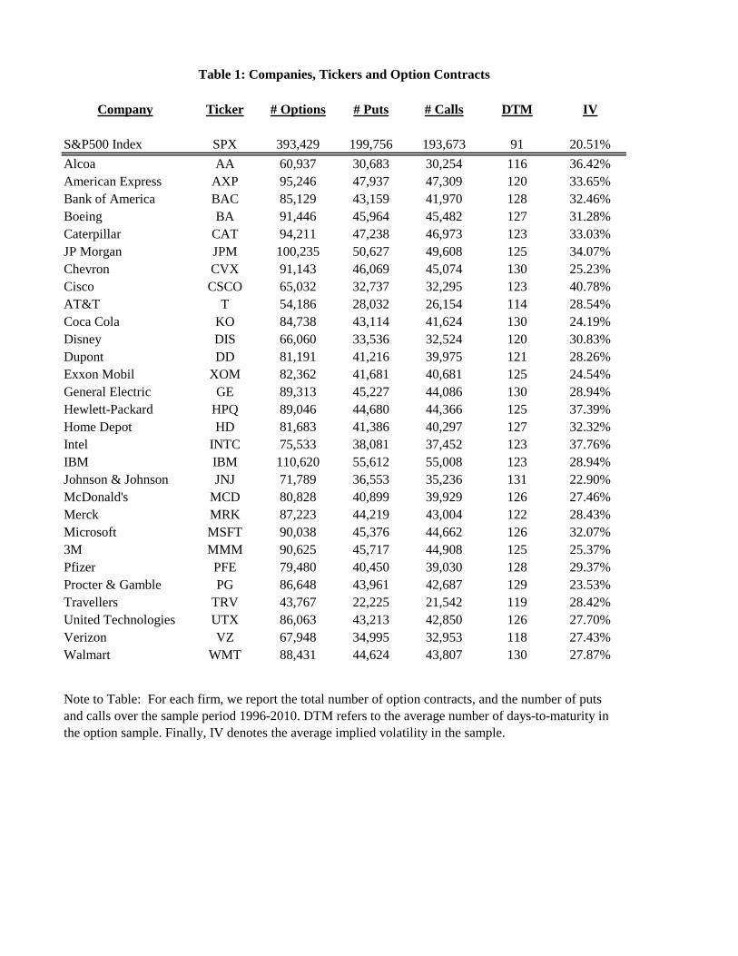
Table 1 presents the number of option contracts, the number of calls and puts, the average days-

to-maturity, and the average implied volatility. The S&P500 index has by far the greatest number

of option contracts. We have a total of 393; 429 index option contracts and 2; 370; 951 equity option

contracts across the 29 �rms. The market average implied volatility is 20:51% during the study

period. Cisco has the highest average implied volatility (40:78%) while Johnson & Johnson has the

smallest (22:89%). Table 1 also shows that our data set is balanced with respect to the number of

OTM calls and puts retained.

Table 2 reports the average, minimum, and maximum implied volatility, as well as the average

option vega. Note that apart from Cisco the average implied volatilities of OTM puts are always

higher than the average implied volatilities of OTM calls.

Figure 1 plots the daily average short-term (9 < DTM < 60) at-the-money (0:95 < S=K < 1:05)

4

implied volatility (IV) for six �rms (black lines) as well as for the S&P500 index (grey lines). Figure

1 shows that the short-term at-the-money (ATM) equity volatility for each �rm has a large part of

its variation driven by the S&P500 index

2.2 Methodology

We want to assess the extent to which the time-varying volatilities of equities share one or more

common components. In order to gauge the degree of commonality in risk-neutral volatilities, we

need daily estimates of the level and slope of the implied volatility curve, and slope of the term

structure of implied volatility for all �rms and the index. For each day t we run the following

regression for �rm j

IVj;l = aj;t + bj;t ��Sjt =Kj;l

�+ cj;t � (DTMj;l) + �j;l

where l denotes the contracts available for �rm j on day t, and for which the regressors are stan-

dardized daily (i.e. we subtract the mean and divide by the standard deviation). We interpret aj;tas a measure of the level of implied volatilites of �rm j on day t. Similarly, bj;t captures the slope

of implied volatility curve while cj;t proxies for the slope of the term structure of implied volatility.

Once we obtain the aj;t, bj;t and cj;t for every day t and �rm j, we then match our daily estimates

for the 29 �rms. In order to reduce the noise in our measures of the slope of implied volatility curve

and term structure, we construct a 10-day moving-average of the bj;t and cj;t. We repeat the same

procedure for the index. Armed with our equity time-series proxies for the level, and slopes of

implied volatility curve and term structure, we rely on principal component analysis (PCA) to

extract common factors. For each proxies (i.e. a, b, and c), we investigate the extent to which the

S&P500 corresponding time-series relate to the �rst three principal components exctracted.

2.2.1 Common Factors in the Level of Implied Equity Volatility

Table 3 contains the results. We report the loading of each equity IV on the �rst three compo-

nents. At the bottom of the table we show the average, min and max loading across �rms for each

component. We also report the total variation captured as well as the correlation of each compo-

nent with the S&P500 IV. The results in Table 3 are quite striking. The �rst component captures

66% of the total cross-sectional variation in short-term IV and it has an 88% correlation with the

S&P500 index IV. This suggests that the equity IVs have a very strong common component which

is well-captured by index option IV. Note that the loadings on the �rst component are positive for

all 29 �rms illustrating the pervasive nature of the common factor.

The top panel of Figure 2 shows the time series of short-term IV for index options. The bottom

5

panel plots the time series of the �rst PCA component of equity IV. The strong relationship between

the two series is readily apparent.

The second PCA component in Table 3 explains 21% of the total variation and the third compo-

nent explains 4%. The average loadings on these two components are close to zero and the loadings

take on a wide range of positive and negative values. The sizable second PCA component and

the wide range of loadings show the need for a second source of �rm speci�c variation in equity

volatility.

2.2.2 Common Factors in the Moneyness Slope

Table 4 contains the results. The moneyness slopes contain a perhaps surprisingly high degree

of comovement. The �rst principal component explains 65% of cross-sectional variation in the

moneyness slope. The second and third components explain 15% and 8% respectively. The �rst

component has positive loadings on all 29 �rms where as the second and third components have

positive and negative loadings across �rms, and average loadings very close to zero.

Table 4 also shows that the �rst principal component has an 83% correlation with the moneyness

slope of S&P500 implied volatility. The second and third components have slopes of 2% and 8%

respectively. Equity moneyness slope dynamics clearly seem driven to an important extent by a

market slope factor.

Figure 3 plots the S&P500 index IV moneyness slope in the top panel and the �rst principal

component from the equity moneyness slopes in the bottom panel. While deviations between the

top and bottom panel are apparent the overall relationship is strong. The common component in

equity moneyness slopes is quite closely related to the moneyness slope of index options.

2.2.3 Common Factors in the Term Structure of Implied Equity Volatility

Table 5 contains the results. The term slope variation captured by the �rst principal component is

61%, which is lower than for spot volatility (Table 3) and moneyness slope (Table 4). The loadings

on the �rst component are positive for all 29 �rms. The correlation between the �rst component

and the term slope of S&P500 index option IV is 66% which is quite high but again lower than the

correlations found in Tables 3 and 4. The second and third components capture 16% and 5% of the

variation respectively and the wide range of loadings suggest a scope for �rm-speci�c variation in

the IV term structure for equity options.

Figure 4 plots the S&P500 index IV term structure slope in the top panel and the �rst principal

component from the equity term slopes in the bottom panel. Some of the spikes in S&P500 mon-

eyness slopes are clearly evident in the �rst principal component but the relationship between two

6

series is not as strong as that found for spot volatility (Figure 2) and moneyness slope (Figure 3).

We conclude that while the market volatility term structure captures a substantial share of the

variation in equity volatility term structures, the scope for a persistent �rm-speci�c volatility factor

seems clear.

2.3 Other Stylized Facts of Equity Option Prices

The literature on equity options has documented a number of important stylized facts that are

complementary to our �ndings above.

Dennis and Mayhew (2002) �nd that option-implied skewness tends to be more negative for

stocks with larger betas. Bakshi, Kapadia and Madan (2003) show that the market index volatil-

ity smile is on average more negatively sloped than individual smiles. They also show that the

more negatively skewed the risk-neutral distribution, the steeper the volatility smile. Finally, they

�nd that the risk-neutral equity distributions are on average less skewed to the left than index

distributions.

Duan and Wei (2009) �nd that the level of implied equity volatility is related to the systematic

risk of the �rm and that the slope of the implied volatility curve is related to systematic risk as

well. Driessen, Maenhout and Vilkov (2009) �nd a large negative index variance risk premium, but

�nd no evidence of a negative risk premium on individual variance risk.

We next outline a structural equity option modeling approach that is able to capture these

well-know stylized facts as well as the results from the analysis outlined above.

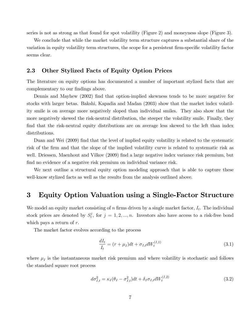
3 Equity Option Valuation using a Single-Factor Structure

We model an equity market consisting of n �rms driven by a single market factor, It. The individual

stock prices are denoted by Sjt , for j = 1; 2; :::; n. Investors also have access to a risk-free bond

which pays a return of r.

The market factor evolves according to the process

dItIt= (r + �I)dt+ �I;tdW

(I;1)t (3.1)

where �I is the instantaneous market risk premium and where volatility is stochastic and follows

the standard square root process

d�2I;t = �I(�I � �2I;t)dt+ �I�I;tdW(I;2)t (3.2)

7

As in Heston (1993), �I denotes the long-run variance, �I captures the speed of mean reversion

of �2I;t to �I and �I measures volatility of volatility. The innovations to market factor return and

volatility are correlated with coe¢ cient �I . Conventional estimates of �I are negative and large

capturing the so-called leverage e¤ect in aggregate market returns.

Individual equity prices are driven by the market factor as well as an idiosyncratic term which

also has stochastic volatility

dSjt

Sjt� rdt = �jdt+ �j

�dItIt� rdt

�+ �j;tdW

(j;1)t (3.3)

d�2j;t = �j(�j � �2j;t)dt+ �j�j;tdW(j;2)t (3.4)

where �j denotes the excess return and �j is the market beta of �rm j.

The innovations to idiosyncratic return and volatility are correlated with coe¢ cient �j. As

suggested by the skew laws derived in Bakshi, Kapadia, and Madan (2003), asymmetry of the idio-

syncratic return component is required to explain the di¤erences in the price structure of individual

equity versus market index options.

Note that our model of the equity market has a total of 2 (n+ 1) innovations.

3.1 Risk Neutral Distribution

In order to use our model of the equity market to value derivatives we need to assume a change

of measure from the physical (P -measure) distribution developed above to the risk-neutral (Q-

measure) distribution. Following the literature, we assume the a stochastic exponential change-of-

measure of the form

dQ

dP(t) = exp

��

tR0

udWu �1

2

tR0

0

udDW;W

0Eu u

�(3.5)

whereWu is a vector containing the 2(n+1) innovations and u is a vector of market prices of risk.6

In the spirit of Cox, Ingersoll, and Ross (1985) and Heston (1993) among others, we assume a

price of market variance risk of the form �I�I;t. We also assume that idiosyncratic variance risk is

not priced. These assumptions enable the following

Proposition 1 Given the change-of-measure in (3.5) the Q-process of the market factor is given

6The exact form of Wu and u are given in Appendix A.

8

by

dItIt

= rdt+ �I;td ~W(I;1)t (3.6)

d�2I;t = ~�I

�~�I � �2I;t

�dt+ �I�I;td ~W

(I;2)t (3.7)

where ~�I = �I + �I�I ; and ~�I =�I�I~�I

(3.8)

and the Q-processes of the individual equities are given by

dSjt

Sjt= rdt+ �j

�dItIt� rdt

�+ �j;td ~W

(j;1)t (3.9)

d�2j;t = �j��j � �2j;t

�dt+ �j�j;td ~W

(j;2)t (3.10)

where d ~Wt denotes the risk-neutral version of dWt

Proof. See Appendix A.These propositions provide several insights. Note that the market factor structure is preserved

under Q. Consequently, the market beta is the same under the risk-neutral and physical dis-

tributions. This is consistent with Serban, Lehoczky, and Seppi (2008) who document that the

risk-neutral and objective betas are economically and statistically close for most stocks.

It is also important to note that in our modeling framework, higher moments (variance, skewness,

and kurtosis) and their premiums, as de�ned by the di¤erence between the level of the moment

under Q with the level under P , are all a¤ected by the drift adjustment in the variance processes.

We will discuss this further below.

3.2 Closed-Form Option Valuation

Our model has been cast in an a¢ ne framework which implies that the characteristic function for

the log market value and the log equity price can both be derived analytically. The market index

characteristic function will be exactly identical to that in Heston (1993). Consider now individual

equity options. We need the following

Proposition 2 The risk-neutral conditional characteristic function ~�t;T (u) for the equity price isgiven by

~�t;T (u) � EQt�exp

�iu ln

�SjT���

(3.11)

=�Sjt�iuexp

�iur (T � t)� AI

��S; u

��BI

��S; u

��2I;t � Aj

��S; u

��Bj

��S; u

��2j;t�

9

where the expressions for �S; AI��S; u

�, BI

��S; u

�, Aj

��S; u

�, and Bj

��S; u

�are provided in

Appendix C.

Proof. See Appendix B.Given the log spot price characteristic function under Q, the price of a European equity call

option with strike price K and maturity T � t is

Cjt (K;T � t) = Sjt�1 �Ke�r(T�t)�2 (3.12)

where the risk-neutral probabilities �1 and �2 are de�ned by7

�1 =1

2+e�r(T�t)

�Sjt

1R0

Re

"e�iu lnK~�t;T (u� i)

iu

#du (3.13)

�2 =1

2+1

�

1R0

Re

"e�iu lnK~�t;T (u)

iu

#du (3.14)

While these integrals must be evaluated numerically, they are well-behaved and can be computed

quickly.

4 Model Properties and Implications

In this section we derive a number of important implications from our model and assess if the model

captures the stylized facts observed in equity option prices in Section 2. For convenience we will

assume that beta is positive for each �rm below. This is not required by the model but it simpli�es

certain expressions.

4.1 Equity Option Volatility Level

Duan and Wei (2009) show empirically that �rms having a higher systematic risk tend to have

a higher level of risk-neutral variance. We now investigate if our model is consistent with this

empirical �nding.

First, de�ne total spot variance for �rm j at time t

Vj;t � �2j�2I;t + �2j;t7A formal proof of this result can be found in Wu (2008).

10

and de�ne the corresponding integrated variance by

Vj;t:T �Z T

t

Vj;sds

Given our model, the integrated total variance for equity j under Q is

~Vj;t:T = �2j ~�2I;t:T + ~�

2j;t:T = �

2j ~�2I;t:T + �

2j;t:T

where ~Vj;t:T , ~�2I;t:T , and �2j;t:T correspond to the integrated variances from t to T . Note that the

second equation holds as long as idiosyncratic risk is not priced.

For any two �rms having the same level of total variance under the P -measure (V1;t:T = V2;t:T )

we have

�21;t:T � �22;t:T = �(�21 � �22)�2I;t:T

As a result:

~V1;t:T � ~V2;t:T = (�21 � �22)~�2I;t:T +��21;t:T � �22;t:T

�= (�21 � �22)

�~�2I;t:T � �2I;t:T

�When the market variance premium is negative, we have ~�I > �I which implies that ~�2I;t:T > �

2I;t:T .

We therefore have that

�1 > �2 , ~V1;t:T > ~V2;t:T

We conclude that our model predicts the �nding in Duan and Wei (2009) that �rms with high betas

tend to have a high level of risk-neutral variance.

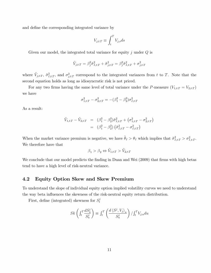
4.2 Equity Option Skew and Skew Premium

To understand the slope of individual equity option implied volatility curves we need to understand

the way beta in�uences the skewness of the risk-neutral equity return distribution.

First, de�ne (integrated) skewness for Sjt

Sk

�R Tt

dSjuSju

��R Tt

�d hSj; Vjiu

Sju

�=R TtVj;udu

11

and let the proportion of systematic risk in �rm j be de�ned by

Aj;t:T ��2j�

2I;t:T

Vj;t:T

Our model implies that the total skewness of individual equity Sjt takes the form

TSkj = SkI � A3=2j;t:T + Skj � (1� Aj;t:T )3=2 (4.1)

where TSkj = Sk�R T

tdSjsSjs

�; SkI = Sk

�R TtdIsIs

�; and Skj = Sk

�R Tt�j;sdW

(j;1)s

�.

The TSkj expression shows that �j determines the loading of security j on market skewness

by a¤ecting how total variance is decomposed into systematic and idiosyncratic risk. Therefore, �ja¤ects the slope of implied volatility curve for the equity. The expression also shows how changes

in market skewness will a¤ect the slope of individual equity implied volatility curve.

The market variance risk premium is negative and as a result, the proportion of systematic risk

strictly increases going from P to Q. This in turn suggests that equity return moments are more

a¤ected by changes in the systematic skewness under the Q measure than under the P measure.

Consequently, the market variance premium can potentially explain the co-movements in the equity

implied volatility slopes found for individual equity options in Section 2.

Consider two �rms having the same quantity of total physical variance and �1 > �2 then

A1;t:T > A2;t:T . As a result, �rm 1 has a greater loading on the index skewness than �rm 2. In a

market where the index Q-distribution is highly negatively skewed while the idiosyncratic equity

distribution is only mildly negatively skewed, we will have the following cross-sectional prediction:

higher-beta �rms will have more negatively skewed Q-distributions. Note that this prediction is in

line with the cross-sectional empirical �ndings of Duan and Wei (2009) and Dennis and Mayhew

(2002).

Using the model we can show that the skewness premium of an individual equity Sjt takes the

form gTSkj � TSkj = hfSkI � Skji ~A3=2j;t:T � [SkI � Skj]A3=2j;t:TRecall that when the market variance risk premium is negative, we have ~Aj;t:T > Aj;t:T . Beta

increases the proportion of systematic risk, Aj;t:T . A negative market skewness premium combined

with the fact that ~Aj;t:T > Aj;t:T implies that when controlling for total variance, high-beta �rms

will have low skewness premiums.

Figure 5 plots the implied Black-Scholes volatility from model option prices. Each line has a

di¤erent beta but the same amount of unconditional total equity variance Vj = �2j�I + �j = 0:1. We

12

set the current spot variance to �2I;t = 0:01 and Vj;t = 0:05, and de�ne the idiosyncratic variance as

the residual �2j;t = Vj;t��2j�2I;t. The market index parameters are �I = 5; �I = 0:04; �I = 0:5; �I =�0:8; and the individual equity parameters are �j = 1; �j = 0:4; and �j = 0. The risk-free rate is4% per year and option maturity is 3 months. Figure 5 shows that beta has a substantial impact

on the moneyness slope of equity IV even when keeping the total variance constant: The higher the

beta the larger the moneyness slope.

4.3 Equity Volatility Term-Structure

We next investigate the model�s implication for the term structure of equity volatility. The role of

the market beta turns out to be crucial.

Our model implies the following two-component term-structure of equity variance

Et( ~Vj;t:T ) =��2j~�I + �j

�+ �2j

��2I;t � ~�I

�e�~�I(T�t) +

��2j;t � �j

�e��j(T�t) (4.2)

This expression shows how the market variance term-structure a¤ects the variance term-structure

for the individual equity. Given di¤erent systematic and idiosyncratic mean reverting speeds (~�I 6=�j), we see that �j has important implications on the term-structure of volatilities. When the

idiosyncratic variance process is more persistent (~�I > �j), higher values of beta imply a faster

reversion toward the long-term total variance horizon (~Vj = �2j~�I + �j). As a result, when the

market variance process is less persistent than the idiosyncratic variance, in the cross-section, �rms

having higher betas are likely to have steeper volatility term-structure. In other words, higher

beta �rms are expected to have a greater positive (resp. negative) slope when the market variance

term-structure is upward (resp. downward) sloping.

Figure 6 plots the implied Black-Scholes volatility from model prices against option maturity.

Each line has a di¤erent beta but the same amount of unconditional total equity variance Vj =

�2j�I + �j = 0:1. We set the current spot variance to �2I;t = 0:01 and Vj;t = 0:05, and de�ne the

idiosyncratic variance as the residual �2j;t = Vj;t � �2j�2I;t. The parameter values are as in Figure 5.Figure 6 shows that beta has a non-trivial e¤ect on the IV term structure: The higher the beta the

steeper the term structure when the term structure is upward sloping.

4.4 Equity Option Risk Management

In classic equity option valuation models, partial derivatives are used to assess the sensitivity of

the option price to the underlying stock price (delta) and equity volatility (vega). In our model

the equity option price additionally is exposed to changes in the market level and market variance.

13

Portfolio managers with well-diversi�ed equity option holdings need to know the sensitivity of the

equity option price to these market level variables in order to properly manage risk. The following

proposition provides the model�s implications for market level sensitivity and market volatility

sensitivity.

Proposition 3 For a derivative contract f j written on the stock price, Sjt , the sensitivity of f j

with respect to market value, It (market delta) is given by:

@f j

@It=@f j

@Sjt

SjtIt�j

The sensitivity of f j with respect to market variance (market vega) takes the form:

@f j

@�2I;t=@f j

@Vj;t�2j

Proof. See Appendix C.

This proposition shows that the beta of the �rm in a straightforward way provides the link

between the usual stock price delta @fj

@Stand the market delta, @f

j

@It, as well as the link between the

usual equity vega, @fj

@Vj;t, and the market vega @fj

@�2I;t.

4.5 Equity Option Expected Returns

So far our model implications have focused on option prices. In certain applications, such as option

portfolio management, option returns are of interest as well. Our �nal proposition provides an

expression for the expected (P -measure) equity option return as a function of the expected market

return.

Proposition 4 For a derivative f j written on the stock price, Sjt , the expected excess return on thederivative contract is given by

1

dtEPt�df j=f j � rdt

�=@f j

@It

Itf j�I =

@f j

@Sjt

Sjtf j�j�I

where @fj

@Itand @fj

@�2I;tare from the Proposition 3.

Proof. See Appendix D.

This proposition reveals that the beta of the stock provides a simple link between the expected

return on the market index and the expected return on the equity option via the delta of the option.

14

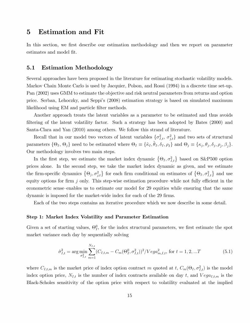
5 Estimation and Fit

In this section, we �rst describe our estimation methodology and then we report on parameter

estimates and model �t.

5.1 Estimation Methodology

Several approaches have been proposed in the literature for estimating stochastic volatility models.

Markov Chain Monte Carlo is used by Jacquier, Polson, and Rossi (1994) in a discrete time set-up.

Pan (2002) uses GMM to estimate the objective and risk neutral parameters from returns and option

price. Serban, Lehoczky, and Seppi�s (2008) estimation strategy is based on simulated maximum

likelihood using EM and particle �lter methods.

Another approach treats the latent variables as a parameter to be estimated and thus avoids

�ltering of the latent volatility factor. Such a strategy has been adopted by Bates (2000) and

Santa-Clara and Yan (2010) among others. We follow this strand of literature.

Recall that in our model two vectors of latent variables f�2I;t, �2j;tg and two sets of structuralparameters f�I , �jg need to be estimated where �I � f~�I ; ~�I ; �I ; �Ig and �j � f�j; �j; �j; �j; �jg.Our methodology involves two main steps.

In the �rst step, we estimate the market index dynamic��I ; �

2I;t

based on S&P500 option

prices alone. In the second step, we take the market index dynamic as given, and we estimate

the �rm-speci�c dynamics��j; �

2j;t

for each �rm conditional on estimates of

��I ; �

2I;t

and use

equity options for �rm j only. This step-wise estimation procedure�while not fully e¢ cient in the

econometric sense�enables us to estimate our model for 29 equities while ensuring that the same

dynamic is imposed for the market-wide index for each of the 29 �rms.

Each of the two steps contains an iterative procedure which we now describe in some detail.

Step 1: Market Index Volatility and Parameter Estimation

Given a set of starting values, �0I , for the index structural parameters, we �rst estimate the spot

market variance each day by sequentially solving

�̂2I;t = argmin�2I;t

NI;tXm=1

(CI;t;m � Cm(�0I ; �2I;t))2=V ega2m;I;t, for t = 1; 2; :::T (5.1)

where CI;t;m is the market price of index option contract m quoted at t, Cm(�I ; �2I;t) is the model

index option price, NI;t is the number of index contracts available on day t; and V egaI;t;m is the

Black-Scholes sensitivity of the option price with respect to volatility evaluated at the implied

15

volatility. These vega-weighted dollar price errors are a good approximation to implied volatility

errors and they are much more quickly computed.8

Once the set of T market spot variances have be obtained we solve for the set of market para-

meters as follows

�̂I = argmin�I

NIXm;t

(CI;t;m � Cm(�I ; �̂2I;t))2=V ega2I;t;m, (5.2)

where NI �PT

t NI;t represents the total number of index option contracts available.

We iterate between (5.1) and (5.2) until the improvement in �t is negligible which typically

requires 5-10 iterations.

Step 2: Equity Volatility and Parameter Estimation

Given an initial value �0j and using the estimated �̂2I;t and �̂I we can estimate the spot equity

variance each day by sequentially solving

�̂2j;t = argmin�2j;t

Nj;tXm=1

(Cj;t;m � Cm(�0j ; �̂I ; �̂2I;t; �2j;t))2=V ega2j;t;m, for t = 1; 2; :::T (5.3)

where Cj;t;m is the price of equity option m for �rm j quoted at t, Cm(�j;�I ; �2I;t; �2j;t) is the model

equity option price, Nj;t is the number of equity contracts available on day t; and V ega;j;t;m is the

Black-Scholes Vega of the equity option.

Once the set of T market spot variances have be obtained we solve for the set of market para-

meters as follows

�̂j = argmin�j

NjXm;t

(Cj;t;m � Cm(�j; �̂I ; �̂2I;t; �̂2j;t))=V ega2j;t;m (5.4)

where Nj �PT

t Nj;t is the total number of contract available for security j.

We again iterate between (5.3) and (5.4) until the improvement in �t is negligible.

5.2 Estimation Results

This section presents results from the market index and 29 equity option model estimations. The

nonlinear least squares estimation is computationally intensive and so we use option data for 2002-

2005 only. For equity options we use contracts on each trading day. For index options we estimate

8This approximation has been used in Carr and Wu (2007) and Trolle and Schwartz (2009) among others.

16

the structural parameters in (5.2) on Wednesday data only because the computational burden is

exorbitantly large if all trading days are used.

Our S&P500 index options are European, but our individual equity options are American style.

As a result, their prices are in�uenced by early exercise premiums. To circumvent possible biases

in our implied volatility estimates due to the presence of both early exercise premia and dividends,

we eliminate in-the-money (ITM) options for which the early exercise premium matters most.9

Table 6 reports estimates of the structural parameters that describe the dynamic of the system-

atic variance, the beta of each �rm, as well as the idiosyncratic variance dynamics. The top row

shows estimates for the S&P500 index.

The unconditional market variance ~�I = 0:0403 corresponds to 20% volatility per year. The

idiosyncratic �j estimates range from 0:0101 for Dupont to 0:0996 for Microsoft.

The market index variance speed of mean-reversion parameter ~�I = 3:20 corresponds to a daily

variance persistence of 1 � 3:20=365 = 0:991. The idiosyncratic �j range from 0:42 for United

Technologies to 3:29 for P�zer showing that idiosyncratic volatility is highly persistent as well.

Interestingly, Dupont and P�zer are the only two �rms of our cross-section having an idiosyncratic

variance process less persistent than the market one.

As typically found in the literature, �I = �0:736 is strongly negative capturing the so-calledleverage e¤ect in the market index. The idiosyncratic �j are also strongly negative ranging from

�0:947 for Hewlett-Packard to �0:579 for Bank of America. The equity option data clearly requireadditional option skewness from the idiosyncratic volatility component.

The estimates of beta vary from 0:75 for Microsoft to 1:33 for Alcoa. The average beta across

the 29 �rms is 1:03.

5.3 The Cross-Section of Volatility, Skewness, and the Slope of the

Volatility Term Structure

The three central predictions of our model, as discussed in Section 4, are as follows:

1. Firms with higher betas have higher risk-neutral variance.

2. Firms with higher betas have larger moneyness slopes. This is equivalent to stating that �rms

with higher betas are characterized by more negative skewness.

9Table 2 in Bakshi, Kapadia, and Madan (2003) shows that for OTM calls and puts, the di¤erence betweenBlack-Scholes implied volatilities and American option implied volatilities (early excercise premia) are negligible.Elkamhi and Ornthanalai (2010) get a similar result. See also Duan and Wei (2009).

17

3. Firms with higher betas have steeper positive volatility term structures when the term struc-

ture is upward sloping, and steeper negative volatility term structures when the term structure

is downward sloping.

We now document how these theoretical model implications are captured by the estimates for

the 29 Dow-Jones �rms. Table 7 reports the relevant estimates. The �rst column of Table 7 lists

the betas for the 29 �rms. The second column of Table 7 reports the average spot volatility for

each �rm de�ned by

ASVj �r1

T

XT

t=1

��2j�

2I;t + �

2j;t

�The average total spot volatility ranges from 19:13% for Procter & Gamble to 42:16% for Cisco.

The top panel of Figure 7 graphically represents the relationship between �j and ASVj. The

cross-sectional relationship is clearly positive. This is con�rmed by the slope of the regression line

(b=0:22). Note the 57% correlation between �j and ASVj (see Table 7) which con�rms that higher

beta �rms have higher total variance.

We now document the cross-sectional relation between beta and the moneyness slope. Because

computing the slope necessitates ancillary assumptions, we document the relationship between beta

and skewness, which is the main determinant of the moneyness slope. The third column of Table 7

reports the average instantaneous skewness de�ned by

AISKj �1

T

XT

t=1

�3j�I�I�

2I;t + �j�j�

2j;t

Vj;t

!

Note that this measure is a function of both the structural parameters as well as the estimated

path of the spot variances. The correlation between skewness and beta is �43%. This negative linkbetween the steepness of the implied volatility curve and beta is evident from the middle panel of

Figure 7 with an estimated slope of �0:12. This negative relationship between skewness and betacon�rms the second model implication that �rms with higher betas have larger moneyness slopes.

Finally, the bottom panel of Figure 7 documents the cross-sectional link between beta and the

steepness of the volatility term structure. As previously mentioned, the model makes predictions

for both upward and downward sloping term-structures. In order to capture the e¤ect of beta

on the slope of the term-structure into one testable hypothesis, we de�ned the average absolute

term-structure slope for each �rm (fourth column in Table 7). This measure is constructed as

follow

AATSj �1

T

XT

t=1abs[�~�I�2j

��2I;t � ~�I

�e�~�I0:25 � �j

��2j;t � �j

�e��j0:25]

18

where the term inside the absolute operator corresponds to a daily estimate of the slope of the

variance term-structure evaluated at T = 0:25 (i.e. @Et( ~Vj;t:T )

@T T=0:25). For every �rm and every day,

we compute the absolute term-structure slope. We then average our daily estimates over the entire

sample period. The cross-sectional correlation between �j and AATSj is 55%. The bottom panel

of Figure 7 visually represents this cross-sectional relationship with an estimated slope of 0:08.

We conclude that our estimates strongly con�rm the three main model implications. We next

address the important question how well we �t the data while capturing these cross-sectional rela-

tionships.

5.4 Model Fit

Wemeasure model �t using the vega root mean squared error (RMSE) de�ned from the optimization

criteria function as

Vega RMSE �r1

N

XN

m;t(Cm;t � Cm;t(�))2=V ega2m;t

We also report the implied volatility RMSE de�ned as

IVRMSE �r1

N

XN

m;t(IVm;t � IV (Cm;t(�)))2

where IVm;t denotes market IV for option m on day t and IV (Cm;t(�)) denotes model IV. Finally,

we report IV bias de�ned by

IV Bias � 1

N

XN

m;tIVm;t �

1

N

XN

m;tIV (Cm;t(�))

We use Black-Scholes to compute IV everywhere in this section.

Table 8 reports model �t for the market index and for each of the 29 �rms. We report results for

all contracts as well as for our OTM calls and puts separately. Several interesting �ndings emerge.

First, the vega RMSE approximates the IVMRSE closely for the index and for all �rms. Second,

the S&P500 index has a good �t with an IVRMSE of 0:91%: Third, the best pricing performance

for equity options is obtained for Coca Cola with an IVRMSE of 1:20%. The worst �t is for JP

Morgan where the IVRMSE is 2:21%. Part of this result is driven by relatively high IVs for JP

Morgan and low IVs for Coca Cola as Table 1 showed.

Fourth, the average IVRMSE �t across �rms for calls is 1:45% and for puts it is 1:55%. Using

this metric the model �ts OTM calls and puts roughly equally well. Fifth, the IV Bias results show

that the model tends to overprice OTM equity calls and underprice OTM equity puts. This could

19

be driven by an insu¢ cient adjustment for the early exercise premium which a¤ects mostly puts or

alternatively absence of jumps in returns in the model. Allowing for return jumps in the model is

a worthy topic for future study.

6 Summary and Conclusions

Our principal component analysis has revealed a strong factor structure in equity option prices.

The �rst common component explains roughly 66% of the cross-sectional variation in IV and the

common component has an 88% correlation with the short-term implied volatility constructed from

S&P500 index options. Roughly 65% of the variation in the equity skew is captured by the �rst

principal component. This common component has a correlation of 83% with the skew of market

index options. When looking for a common component in the term structure of equity IV we �nd

that 61% of the variation is explained by the �rst principal component. This component has a

correlation of 66% with the term slope of the option IV from S&P500 index options.

Motivated by the �ndings from the principal component analysis, we develop a structural model

of equity option prices that incorporates a market factor. Our model allows for mean-reverting

stochastic volatility and correlated shocks to return and volatility. Motivated by our principal com-

ponents analysis we allow for idiosyncratic shocks to equity prices which also have mean-reverting

stochastic volatility and a separate leverage e¤ect. Individual equity returns are linked to the

market index using a standard linear factor model with a constant beta factor loading. We de-

rive closed-form option pricing formulas as well as results for option hedging and option expected

returns.

We have also developed a convenient estimation method for estimation and �ltering based on

option prices. When estimating the model on the �rms in the Dow we �nd that it provides a good

�t to observed equity option prices. Moreover, we show that our estimates strongly con�rm the

three main cross-sectional model implications.

Several issues are left for future research. First, it would be interesting to allow for two stochastic

volatility factors in the market price process. Second, allowing for jumps in the market price as well

as in the idiosyncratic shock would be relevant. Finally, using the model to construct option-implied

betas for use in cross-sectional equity pricing could be of substantial interest.

Appendix

This appendix collects the proofs of our four propositions.

20

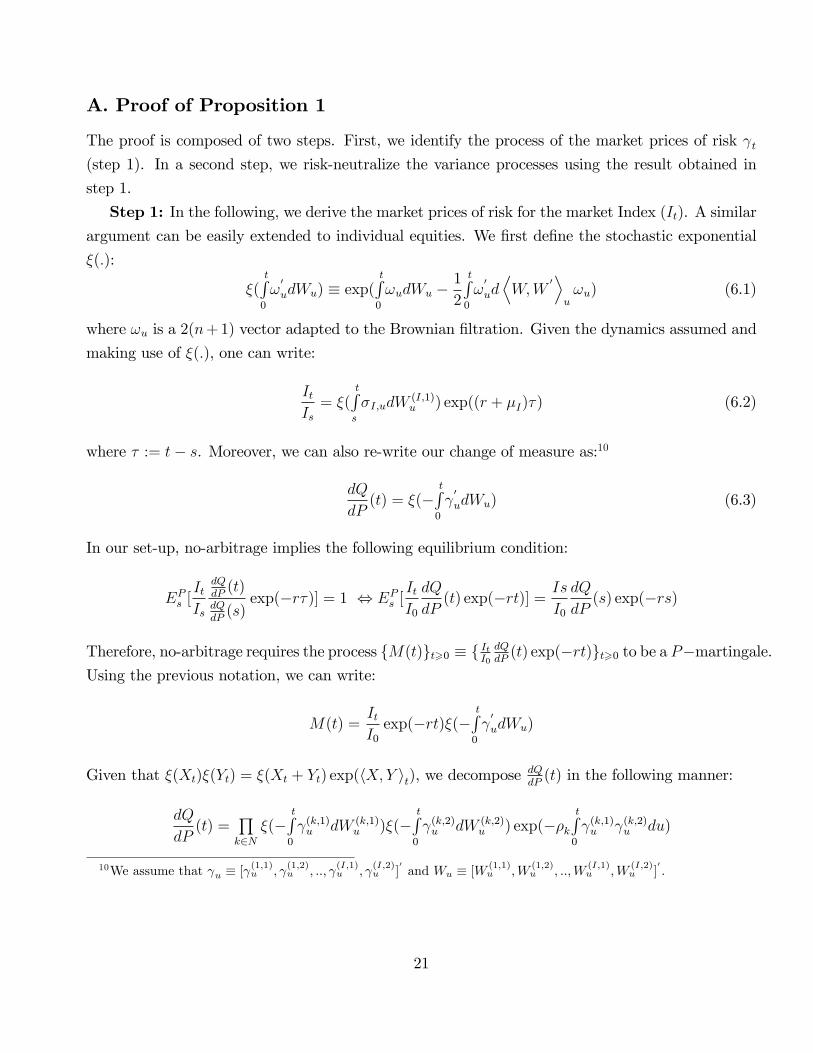
A. Proof of Proposition 1

The proof is composed of two steps. First, we identify the process of the market prices of risk t(step 1). In a second step, we risk-neutralize the variance processes using the result obtained in

step 1.

Step 1: In the following, we derive the market prices of risk for the market Index (It). A similarargument can be easily extended to individual equities. We �rst de�ne the stochastic exponential

�(:):

�(tR0

!0

udWu) � exp(tR0

!udWu �1

2

tR0

!0

udDW;W

0Eu!u) (6.1)

where !u is a 2(n+1) vector adapted to the Brownian �ltration. Given the dynamics assumed and

making use of �(:), one can write:

ItIs= �(

tRs

�I;udW(I;1)u ) exp((r + �I)�) (6.2)

where � := t� s. Moreover, we can also re-write our change of measure as:10

dQ

dP(t) = �(�

tR0

0

udWu) (6.3)

In our set-up, no-arbitrage implies the following equilibrium condition:

EPs [ItIs

dQdP(t)

dQdP(s)exp(�r�)] = 1 , EPs [

ItI0

dQ

dP(t) exp(�rt)] = Is

I0

dQ

dP(s) exp(�rs)

Therefore, no-arbitrage requires the process fM(t)gt>0 � f ItI0dQdP(t) exp(�rt)gt>0 to be a P�martingale.

Using the previous notation, we can write:

M(t) =ItI0exp(�rt)�(�

tR0

0

udWu)

Given that �(Xt)�(Yt) = �(Xt + Yt) exp(hX;Y it), we decomposedQdP(t) in the following manner:

dQ

dP(t) =

Qk2N

�(�tR0

(k;1)u dW (k;1)u )�(�

tR0

(k;2)u dW (k;2)u ) exp(��k

tR0

(k;1)u (k;2)u du)

10We assume that u � [ (1;1)u ;

(1;2)u ; ::;

(I;1)u ;

(I;2)u ]

0and Wu � [W (1;1)

u ;W(1;2)u ; ::;W

(I;1)u ;W

(I;2)u ]

0.

21

Let us de�ne dQdP(t)?It the orthogonal part of the Radon-Nikodym derivative to It:

dQ

dP(t)?It �

Qk2NnfIg

�(�tR0

(k;1)u dW (k;1)u )�(�

tR0

(k;2)u dW (k;2)u ) exp(��k

tR0

(k;1)u (k;2)u du)

Note that dQdP(t)?It is itself a P�martingale. We can now write dQ

dP(t) as:

dQ

dP(t) = �(�

tR0

(I;1)u dW (I;1)u )�(�

tR0

(I;2)u dW (I;2)u ) exp(��I

tR0

(I;1)u (I;2)u du)dQ

dP(t)?It

Using previous notations M(t) can be easily re-written as:

M(t) = F (t)dQ

dP(t)?It

where

F (t) � exp(�It)�(tR0

�I;udW(I;1)u )�(�

tR0

(I;1)u dW (I;1)u )�(�

tR0

(I;2)u dW (I;2)u ) exp(��I

tR0

(I;1)u (I;2)u du)

For M(t) to be a P�martingale, it must be that F (t) is itself a P�martingale. Given the aboveproperty of stochastic exponentials:

�(tR0

�I;udW(I;1)u )�(�

tR0

(I;1)u dW (I;1)u ) = �(

tR0

(�I;u � (I;1)u )dW (I;1)u ) exp(�

tR0

(�I;u (I;1)u )du)

and

�(tR0

(�I;u � (I;1)u )dW(I;1)u )�(�

tR0

(I;2)u dW

(I;2)u ) = �(

tR0

f(�I;u � (I;1)u )dW(I;1)u � (I;2)u dW

(I;2)u g):::

exp(��ItR0

(I;2)u (�I;u � (I;1)u )du)

As a result, F (t) can be expressed as

F (t) = �(tR0

f(�I;u � (I;1)u )dW (I;1)u � (I;2)u dW (I;2)

u g) exp(tR0

f�I � �I;u( (I;1)u + �I (I;2)u )gdu)

Therefore, using previous results a su¢ cient condition for M(t) to be a P�martingale is

�I � �I;t( (I;1)t + �I

(I;2)t ) = 0 dP dt a:s: (6.4)

22

As mentioned earlier, this economy is incomplete and there exist a multitude of combinations

f (I;1)t ; (I;2)t gt>0 satisfying the previous restriction and the Novikov condition.11 In order to obtain

closed-form solution for the characteristic function of f�I;tgt>0 , the literature has imposed themarket price of variance risk (W (I;2)

t ) to be proportional to �I;t :

(I;2)t + �I

(I;1)t = �I�I;t (6.5)

The two last equations uniquely de�ne (I;1)t and (I;2)t . A similar argument can be used for individual

equity with the restriction: (j;2)t + �j (j;1)t = 0. Combining previous results, the Girsanov theorem

and the properties of Lévy processes implies that the vector ~Wt of Q-Brownian motions satis�ed

the following dynamic

d ~Wt = dWt + dDW;W

0Et t (6.6)

where the prices of systematic risk are

(I;1)t =

�I � �I�I�2I;t�I;t(1� �2I)

and (I;2)t =

�I�2I;t � �I�I

�I;t(1� �2I)

and the prices of idiosyncratic risk are

(j;1)t =

�j�j;t(1� �2j)

and (j;2)t = �

�j�j

�j;t(1� �2j)

Step 2: In the following, we present the index return and variance processes risk-neutralization.The same argument applies in regards of individual equities. We know that the index P -dynamic

isdItIt= (r + �I)dt+ �I;tdW

(I;1)t

Making use of the expressions de�ning the Q-Brownian motions, we can re-write this SDE as

dItIt= (r + �I)dt+ �I;t(d ~W

(I;1)t � ( (I;1)t + �I

(I;2)t ))

where (I;1)t and (I;2)t are de�ned in step 1. As a result,

) dItIt= rdt+ (�I � �I;t(

(I;1)t + �I

(I;2)t ))dt+ �I;td ~W

(I;1)t

11We further assume the (su¢ cient) Novikov criterion EP [exp(12tR0

0

udDW;W

0Eu u)] <1 P�a:s: for all t implying

that dQdP (t) is uniformly integrable which ensures the equivalence of the two laws: P � Q, see Protter (1990) III Chp8.

23

and since

(I;1)t + �I

(I;2)t =

�I�I;t

we havedItIt= rdt+ �I;td ~W

(I;1)t

The P -dynamic for the systematic variance process is:

d�2I;t = �I(�I � �2I;t)dt+ �I�I;tdW(I;2)t

By the Girsanov theorem d ~W(I;2)t = (

(I;2)t + �I

(I;1)t )dt+ dW

(I;2)t and therefore:

d�2I;t = �I(�I � �2I;t)dt+ �I�I;t(d ~W(I;2)t � ( (I;2)t + �I

(I;1)t ))

or given

(I;2)t + �I

(I;1)t = �I�I;t

) d�2I;t = ~�I(~�I � �2I;t)dt+ �I�I;td ~W

(I;2)t

where

~�I = �I + �I�I and ~�I =�I�I~�I

B. Proof of Proposition 2

In the following, we focus on the derivation of the call option price for individual equity. Note that

the model of Heston (1993) can be obtained by setting �j = 0, Sjt = It, and all the idiosyncratic

variance parameters equal to the market variance ones. For ease of notation, we de�ne Lkt;T �TRt

�2k;udu and WmLkt;T

�TRt

�k;ud ~W(k;m)u for m 2 f1; 2g and k 2 N . Given the Q -processes, one can

apply Ito�s lemma to obtain the following expression for the individual equity log-returns under Q:

log(SjTSjt) = r (T � t)� 1

2(Ljt;T + �2jLIt;T ) +W 1

Ljt;T+ �jW

1LIt;T

(6.7)

We begin by setting-up the required notation. ~�LR

t;T (:) represents the conditional characteristic

function of the risk-neutral process followed by the log-returns ln(SjT

Sjt). Moreover, we de�ne �S �

24

f~�I ; ~�I ; �I ; �I ; �j; �j; �j; �j; �j; r; T � tg, and

~�LR

t;T (�S; u; �2I;t; �

2j;t) � E

Qt [exp(iu ln(

SjTSjt))]

Using 6.7, one may write

, ~�LR

t;T (�S; u; �2I;t; �

2j;t) = E

Qt [exp(iu(r(T � t)�

1

2(Ljt;T + �2jLIt;T ) +W 1

Ljt;T+ �jW

1LIt;T))]

making use of the stochastic exponential �(:) as de�ne in Appendix A:

, ~�LR

t;T (�S; u; �2I;t; �

2j;t) = exp(iur(T�t))E

Qt [�(iu�jW

1LIt;T) exp(�g1(u)LIt;T )�(iuW 2

Ljt;T) exp(�g2(u)Ljt;T )]

, ~�LR

t;T (�S; u; �2I;t; �

2j;t) = exp(iur(T�t))E

Qt [�(iu�iW

1LIt;T) exp(�g1(u)LIt;T )]E

Qt [�(iuW

1Ljt;T) exp(�g2(u)Ljt;T )]

where g1(u) = iu2�2j(1� iu) and g2(u) = iu

2(1� iu). In the spirit of Carr and Wu (2004) or Detemple

and Rindisbacher (2010), we de�ne the following measure change:

C(t) � EQt [dC

dQ] = �(iu�jW

1LIt)�(iuW 1

Ljt)

where

�(iu�W 1Lkt) = exp(iu�W 1

Lkt� (iu�)

2

2

W 1Lk ;W

1Lk�t) = exp(iu�W 1

Lkt� 12(iu�)2Lkt )

for � 2 R and k 2 fI; jg. Note that C(t) is aQ-martingale with respect to the �ltration generated byf(W 1

LIt;LIt ); (W 1

Ljt;Ljt)gt>0 and is de�ned on the complex plane (see Carr andWu (2004) for a rigorous

treatment of this result for Lévy processes). The fact thatW 1LI ;LI

�t6= 0 and

W 1Lj ;Lj

�t6= 0

renders the search for ~�LR

t;T (:) non-trivial under Q. However, under the C-measure the problem is

greatly simpli�ed. This new measure allows us to write:

, ~�LR

t;T (�S; u; �2I;t; �

2j;t) = exp(iur(T � t))E

Qt [C(T )

C(t)�(iu�iW

1LIt;T) exp(�g1(u)LIt;T )]:::

EQt [C(T )

C(t)�(iuW 1

Ljt;T) exp(�g2(u)Ljt;T )]

) ~�LR

t;T (�S; u; �2I;t; �

2j;t) = exp(iur(T � t))ECt [exp(�g1(u)LIt;T )]ECt [exp(�g2(u)L

jt;T )] (6.8)

25

Given an extension of the Girsanov-Meyer theorem to the complex plane, under the C-measure we

have:

dWC;(I;2)t = d ~W

(I;2)t � (iu�I�j�I;t)dt

dWC;(j;2)t = d ~W

(j;2)t � (iu�j�j;t)dt

As a result, for all k 2 N

d�2k;t = �Ck (�

Ck � �2k;t)dt+ �k�k;tdW

C;(k;2)t (6.9)

where

�CI = ~�I � iu�I�j�I ; �CI =~�I~�I�CI

; �Cj = �j � iu�j�j; and �Cj =�j�j�Cj

Wemake use of the closed-form for the moment generating function of ECt [exp(�g(u)Lt;T )] to obtainan expression for ~�

LR

t;T (:):

~�LR

t;T (�S; u; �2I;t; �

2j;t) = exp(iur(T�t)�AI(�S; u)�BI(�S; u)�2I;t�Aj(�S; u)�Bj(�S; u)�2j;t) (6.10)

with

BI(�S; u) =2g1(u)(1� e�

I(�S ;u)(T�t))

2I(�S; u)� (I(�S; u)� �CI )(1� e�I(�S ;u)(T�t))

(6.11)

AI(�; u) =~�I~�I

�2I

�2 ln(1� (

I(�S; u)� �CI )2I(�S; u)

(1� e�I(�S ;u)(T�t))) + (I(�S; u)� �CI )(T � t)�(6.12)

and

Bj(�S; u) =2g2(u)(1� e�

j(�S ;u)(T�t))

2j(�S; u)� (j(�S; u)� �Cj )(1� e�j(�S ;u)(T�t))

(6.13)

Aj(�S; u) =�j�j

�2j

(2 ln(1�

(j(�S; u)� �Cj )2j(�S; u)

(1� e�j(�S ;u)(T�t))) + (j(�S; u)� �Cj )(T � t))

(6.14)

and where

I(�S; u) =q(�CI )

2 + 2�2Ig1(u) and j(�S; u) =q(�Cj )

2 + 2�2jg2(u)

with

g1(u) =iu

2�2j(1� iu) and g2(u) =

iu

2(1� iu)

Using the fact that ~�t;T (u) = eiu ln(St)~�

LR

t;T (u) then one can use the previous equations to compute

26

the price of a call written on Sjt .

C. Proof of Proposition 3

Within our model, the index price (IT ) take the form:

ItI0= B(t)k(�2I;0:t) exp(X0;t)

where

B(t) � exp(rt), k(a) � exp(�a2); and X0;t �

Z t

0

�I;udW(I;1)u

Taking the derivative of the index price It with respect to �jX0;t gives:

@It@�jX0;t

=It�j

Moreover, within our model the equity price is given by:

Sjt

Sj0= B(t)k(Vj;0:t) exp(�jX0;t) exp(

Z t

0

�j;udW(j;1)u )

Therefore,@Sjt

@�jX0;t

= Sjt

Note that chain rule implies@Sjt@It

=@Sjt

@�jX0;t

@�jX0;t

@It

We know from Malliavin calculus that It is a di¤erentiable function with respect to �jX0;t (see Di

Nunno, Øksendal, Proske, 2008) with non-zero derivative. As a result, the inverse function theorem

implies that:@�jX0;t

@It=

1@It

@�jX0;t

)@�jX0;t

@It=�jIt

Therefore,@Sjt@It

=SjtIt�j )

@f j

@It=@f j

@Sjt

@Sjt@It

=@f j

@Sjt

SjtIt�j

27

From a vega point of view, we have:

@f j

@�2I;t=@f j

@Vj;t

@Vj;t@�2I;t

=@f j

@Vj;t

@(�2j�2I;t + �

2j;t)

@�2I;t=@f j

@Vj;t�2j

D. Proof of Proposition 4

Before deriving the main result of the proposition, we de�ne the required notation. Let f jx � @fj

@x,

f jxx � @2fj

@x2and f jxy � @2fj

@x@ydenote the partial derivative with respect to x, the second derivative

with respect to x, and the cross-derivative with respect to x and y. Ito lemma implies that:

df j = f jt dt+1

2f jSSd

Sj; Sj

�t+ f jSVjd

Sj; Vj

�t

+1

2f jVjVjd hVj; Vjit + f

jSd~Sjt + f

jVjdVj;t

Or the Feynman-Kac formula results in

rf j = f jt + fjS

EQt [dSjt ]

dt+ f jVj

EQt [dVj;t]

dt+1

2f jSS

d hSj; Sjitdt

+f jSVjd hSj; Vjit

dt+1

2f jVjVj

d hVj; Vjitdt

whereEQt [dS

jt ]

dt= rSjt

EQt [dVj;t]

dt= �2j~�I(

~�I � �2I;t) + ~�j(~�j � �2j;t)dhSj ;Sji

t

dt= �2j�

2I;t + �

2j;t = Vj;t

dhSj ;Vjit

dt= (�3j�I�I�

2I;t + �j�j�

2j;t)S

jt

dhVj ;Vjitdt

= (�4j�2I�2I;t + �

2j�2j;t)

Using previous expressions, the dynamic of df j can therefore also be written:

df j = frf j � f jSrSt � fjVj(�2j~�I(

~�I � �2I;t) + ~�j(~�j � �2j;t)gdt+f jSdS

jt + f

jVjdVj;t

Moreover, under the objective probability measure (P ), we have the following equalities:

EPt [dSjt ]

dt= (r + �j�I)S

jt

EPt [dVj;t]

dt= �2j�I(�I � �2I;t) + �j(�j � �2j;t)

28

Consequently,

1

dtEPt [

df j

f j� rdt] = f jS

f jEPt [dS

jt � rSjt dt] +

f jVjf j�2jE

Pt [d�

2I;t � ~�I(~�I � �2I;t)dt]

+f jVjf jEPt [d�

2j;t � ~�j(~�j � �2j;t)dt]

which simpli�es to:

1

dtEPt [

df j

f j� rdt] = f jS

Sjtf j�j�I + f

jVj

�2jf j(~�I~�I � �I�I) + f jVj

1

f j(~�j~�j � �j�j) (6.15)

In the previous expression, Q is the risk-neutral distribution de�ned by 3.5. Consistent with Ap-

pendix A, we risk-neutralize the market variance process such that ~�I~�I = �I�I while idiosyncratic

risk is assumed to be not priced (i.e. ~�j = �j and ~�j = �j). Consequently, we obtain:

1

dtEPt [

df j

fE� rdt] = f jS

Sjtf j�j�I = f

jI

Itf j�I

where the second equation makes use of the result in proposition 3.

Note that part of the literature (see Broadie, Chernov, and Johannes, 2009), risk-neutralize the

variance process such that ~�I = �I . Given such a restriction, 6.15 would become

1

dtEP [

df j

fE� rdt] = f jS

Sjtf j�j�I + f

jVj

�2jf j�I(~�I � �I)

Note that the market variance risk-premium is equal to:

EP [d�2I;t]� EQ[d�2I;t] = �I�I�2I;tdt

Therefore, we have:

) �I(~�I � �I) = �I�I�2I;t

Combining the previous results, we �nally obtain:

1

dtEP [

df j

f j� rdt] = f jS

Sjtf j�j�I + f

jVj

�2jf j�I�I�

2I;t:

29

References

[1] Bakshi, G., Cao, C., Z. Chen, Z. (1997) Empirical performance of alternative option pricing

models, Journal of Finance, 52, 2003�2050.

[2] Bakshi, G., Kapadia, N. (2003) Delta-hedged gains and the negative market volatility risk

premium, Review of Financial Studies, 16, 527�566.

[3] Bakshi, G., Kapadia, N., Madan, D. (2003) Stock return characteristics, skew laws, and di¤er-

ential pricing of individual equity options, Review of Financial Studies, 10, 101�143.

[4] Bates, D. (2000) Post-�87 crash fears in the S&P500 futures option market, Journal of Econo-

metrics, 94, 181-238.

[5] Bates, D. (2008) The market for crash risk, Journal of Economic Dynamics and Control, 32,

2291-2321.

[6] Black, F., Scholes, M. (1973) Valuation of options and corporate liabilities, Journal of Political

Economy, 81, 637�654.

[7] Broadie, M., Chernov, M., Johannes, M. (2007) Model speci�cation and risk premiums: evi-

dence from futures options, Journal of Finance, 62, 1453-1490.

[8] Broadie, M. Chernov, M., Johannes, M. (2009) Understanding index option returns, Review of

Financial Studies, 22, 4493-4529.

[9] Buss, A., Vilkov, G., (2012) Measuring equity risk with option-implied correlations, Manu-

script, Goethe University, Frankfurt.

[10] Carr, P., Wu, L. (2004) Time-changed Lévy processes and option pricing, Journal of Financial

Economics, 71, 113�141.

[11] Carr, P., Wu, L. (2007) Stochastic skew in currency options, Journal of Financial Economics,

86, 213�247.

[12] Carr, P., Wu, L. (2009) Variance risk premiums, Review of Financial Studies, 22, 1311�1341.

[13] Chang, B.Y, Christo¤ersen, P., Jacobs, K., Vainberg, G. (2012) Option-implied measures of

equity risk, Review of Finance. forthcoming.

[14] Christensen, B., Prabhala, N. (1998) The relation between implied and realized volatility,

Journal of Financial Economics, 50, p 125�150.

30

[15] Cox, J.C., Ingersoll, J.E., Ross, S.R. (1985) A theory of the term structure of interest rates,

Econometrica, 53, 385�408.

[16] Dennis, P., Mayhew, S. (2002) Risk-neutral skewness: evidence from stock options, Journal of

Financial and Quantitative Analysis, 37, 471�93.

[17] Detemple, J. B., Rindisbacher, M. (2010) Dynamic asset allocation: portfolio decomposition

formula and applications, Review of Financial Studies, 23, p 25�100.

[18] Di Nunno, G., Øksendal, B., Proske, F. (2008) Malliavin calculus for Lévy processes with

applications to Finance, Springer-Verlag.

[19] Driessen, J., Maenhout, P., Vilkov, G. (2009) The price of correlation risk: evidence from

equity options, Journal of Finance, 64, 1377-1406.

[20] Duan, J-C., Wei, J. (2009) Systematic risk and the price structure of individual equity options,

Review of Financial Studies, 22, 1981�2006.

[21] Du¢ e, D., Kan, R. (1996) A yield-factor model of interest rates, Mathematical Finance, 6,

379�406.

[22] Elkamhi, R., Ornthanalai, C. (2010) Market jump risk and the price structure of individual

equity options, Working Paper, Rotman School, University of Toronto.

[23] Heston, S. (1993) Closed-form solution for options with stochastic volatility, with application

to bond and currency options, Review of Financial Studies, 6, 327�343.

[24] Heston, S., Nandi, S. (2000) A closed-form GARCH option pricing model, Review of Financial

Studies, 13, 585�626.

[25] Hull, J., White, A. (1987) The pricing of options on assets with stochastic volatilities, Journal

of Finance, 42, 281�300.

[26] Jacquier, E., Polson, N.G., Rossi, P.E. (1994) Bayesian analysis of stochastic volatility models

(with discussion), Journal of Business and Economic Statistics, 12, 371-417.

[27] Jones, C.S. (2003) The dynamics of stochastic volatility: evidence from underlying and options

markets, Journal of Econometrics, 116, 181�224.

[28] Mo, H., Wu, L. (2007) International capital asset pricing: evidence from options, Journal of

Empirical Finance, 14, 465-498.

31

[29] Pan, J. (2002) The jump risk premia implicit in options: Evidence from an integrated time

Series Study, Journal of Financial Economics, 63, p. 3-50.

[30] Protter, P. (1990) Stochastic integration and di¤erential equations, Springer-Verlag.

[31] Santa-Clara, P., Yan, S. (2010) Crashes, volatility, and the equity premium: lessons from

S&P500 options, Review of Economics and Statistics, 92, 435-451.

[32] Serban, M., Lehoczky, J., Seppi, D. (2008) Cross-sectional stock option pricing and factor

models of returns, Working Paper, CMU.

[33] Trolle, A., Schwartz, E. (2009) Unspanned stochastic volatility and the pricing of commodity

derivatives, Review of Financial Studies, 22, 4423-4461.

[34] Wiggins, J. (1987) Option values under stochastic volatility: theory and empirical evidence,

Journal of Financial Economics, 19, 351-372.

[35] Wu, L. (2008) Modeling �nancial security returns using Lévy processes, Handbooks in Oper-

ations Research and Management Science: Financial Engineering, J. Birge and V. Linetsky

(eds.), Elsevier.

32

Figure 1: Short-Term At-the-money Implied Volatility. Six Equities and the S&P500 Index

1996 2003 2010

20

40

60

80

100Boeing

1996 2003 2010

20

40

60

80

100Coca Cola

1996 2003 2010

20

40

60

80

100Home Depot

1996 2003 2010

20

40

60

80

100Merck

1996 2003 2010

20

40

60

80

100Proctor and Gamble

1996 2003 2010

20

40

60

80

100Walmart

Notes to Figure: We plot the time series of implied volatility for six equities (black) and S&P500

index (grey). On each day we use contracts with between 9 and 60 days to maturity and a moneyness

(S=K) between 0.95 and 1.05. For every trading day and every security, we average the available

implied volatilities to obtain an estimate of short-term at-the-money implied volatility.

33

Figure 2: S&P500 Index Implied Volatility

and the First Principal Component of Implied Equity Volatility

1996 1998 2000 2002 2004 2006 2008 2010

0.2

0.4

0.6

IV L

evel

S&P500 Implied Volatility Level

1996 1998 2000 2002 2004 2006 2008 2010

0.2

0.4

0.6

IV L

evel

First Principal Component of Equity Implied Volatility Level

Notes to Figure: The top panel plots implied volatility from short-term at-the-money (ATM)

S&P500 index options. The bottom panel plots the �rst principal component of implied short-

term ATM implied volatility from options on 29 equities in the Dow.

34

Figure 3: Implied Volatility Moneyness Slopes:

S&P500 Index and Equity First Principal Component

1996 1998 2000 2002 2004 2006 2008 2010

0.015

0.02

0.025

0.03

0.035

IV M

oney

ness

 Slo

peS&P500 Implied Volatility Moneyness Slope

1996 1998 2000 2002 2004 2006 2008 2010

0.015

0.02

0.025

0.03

0.035

IV M

oney

ness

 Slo

pe

First Principal Component of Equity Implied Volatility Moneyness Slope

Notes to Figure: The top panel plots over time the slope of implied volatility with respect to

moneyness from short-term S&P500 index options. The bottom panel plots the �rst principal

component of the implied volatility moneyness slopes from options on 29 equities in the Dow.

35

Figure 4: Implied Volatility Term Structure Slopes:

S&P500 Index and Equity First Principal Component

1996 1998 2000 2002 2004 2006 2008 2010­0.03

­0.02

­0.01

0

0.01

0.02

IV T

erm

 Slo

peS&P500 Implied Volatility Term Slope

1996 1998 2000 2002 2004 2006 2008 2010­0.03

­0.02

­0.01

0

0.01

0.02

IV T

erm

 Slo

pe

First Principal Component of Equity Implied Volatility Term Slope

Notes to Figure: The top panel plots the slope of the implied volatility term structure from S&P500

index options. The bottom panel plots the �rst principal component of the implied volatility term

structure from options on 29 equities in the Dow.

36

Figure 5: Beta and Implied Volatility Across Moneyness. 3-month Equity Options

0.8 0.85 0.9 0.95 1 1.05 1.1 1.15 1.20.23

0.24

0.25

0.26

0.27

0.28

0.29

0.3

0.31

Moneyness (S/K)

 Impl

ied 

Vol

atili

ty

 Beta = 1.4 Beta = 1.2 Beta = 1 Beta = 0.8 Beta = 0.6

Notes to Figure: We plot implied Black-Scholes volatility from model prices. Each line has a

di¤erent beta but the same amount of unconditional total equity variance Vj = �2j�I + �j = 0:1. We

set the current spot variance to �2I;t = 0:01 and Vj;t = 0:05, and de�ne the idiosyncratic variance as

the residual �2j;t = Vj;t��2j�2I;t. The market index parameters are �I = 5; �I = 0:04; �I = 0:5; �I =�0:8; and the individual equity parameters are �j = 1; �j = 0:4; and �j = 0. The risk-free rate is4% per year and option maturity is 3 months.

37

Figure 6: Beta and the Implied Volatility Term Structure. At-the-money Options

0.5 1 1.5 2 2.5 30.22

0.23

0.24

0.25

0.26

0.27

0.28

0.29

0.3

0.31

Years

 Impl

ied 

Vol

atili

ty T

erm

­Stru

ctur

e Term­Structure of Implied Volatility

 Beta = 1.4 Beta = 1.2 Beta = 1 Beta = 0.8 Beta = 0.6

Notes to Figure: We plot implied Black-Scholes volatility from model prices. Each line has a

di¤erent beta but the same amount of unconditional total equity variance Vj = �2j�I + �j = 0:1. We

set the current spot variance to �2I;t = 0:01 and Vj;t = 0:05, and de�ne the idiosyncratic variance as

the residual �2j;t = Vj;t��2j�2I;t. The market index parameters are �I = 5; �I = 0:04; �I = 0:5; �I =�0:8; and the individual equity parameters are �j = 1; �j = 0:4; and �j = 0. The risk-free rate is4% per year.

38

Figure 7: Cross-Section of Volatility, Skewness, and the Slope of the Volatility Term Structure

0.7 0.8 0.9 1 1.1 1.2 1.3 1.40.1

0.2

0.3

0.4

0.5

Beta

ASV

ObservationsASV = a + b * beta

0.7 0.8 0.9 1 1.1 1.2 1.3 1.4­0.4

­0.35

­0.3

­0.25

­0.2

Beta

AISK

ObservationsAISK = a + b * beta

0.7 0.8 0.9 1 1.1 1.2 1.3 1.40.02

0.04

0.06

0.08

0.1

0.12

Beta

AATS

ObservationsAATS  = a + b * beta

Notes to Figure: We plot the cross-sectional regressions of the 29 model implied measures of average

total spot volatility (ASV - top panel), average instantaneous skewness (AISK - middle panel), and

average absolute term-structure slope (AATS - bottom panel) against the estimated betas.

39

Company Ticker # Options # Puts # Calls DTM IV

S&P500 Index SPX 393,429 199,756 193,673 91 20.51%

Alcoa AA 60,937 30,683 30,254 116 36.42%

American Express AXP 95,246 47,937 47,309 120 33.65%

Bank of America BAC 85,129 43,159 41,970 128 32.46%

Boeing BA 91,446 45,964 45,482 127 31.28%

Caterpillar CAT 94,211 47,238 46,973 123 33.03%

JP Morgan JPM 100,235 50,627 49,608 125 34.07%

Chevron CVX 91,143 46,069 45,074 130 25.23%

Cisco CSCO 65,032 32,737 32,295 123 40.78%

AT&T T 54,186 28,032 26,154 114 28.54%

Coca Cola KO 84,738 43,114 41,624 130 24.19%

Disney DIS 66,060 33,536 32,524 120 30.83%

Dupont DD 81,191 41,216 39,975 121 28.26%

Exxon Mobil XOM 82,362 41,681 40,681 125 24.54%

General Electric GE 89,313 45,227 44,086 130 28.94%

Hewlett-Packard HPQ 89,046 44,680 44,366 125 37.39%

Home Depot HD 81,683 41,386 40,297 127 32.32%

Intel INTC 75,533 38,081 37,452 123 37.76%

IBM IBM 110,620 55,612 55,008 123 28.94%

Johnson & Johnson JNJ 71,789 36,553 35,236 131 22.90%

McDonald's MCD 80,828 40,899 39,929 126 27.46%

Merck MRK 87,223 44,219 43,004 122 28.43%

Microsoft MSFT 90,038 45,376 44,662 126 32.07%

3M MMM 90,625 45,717 44,908 125 25.37%

Pfizer PFE 79,480 40,450 39,030 128 29.37%

Procter & Gamble PG 86,648 43,961 42,687 129 23.53%

Travellers TRV 43,767 22,225 21,542 119 28.42%

United Technologies UTX 86,063 43,213 42,850 126 27.70%

Verizon VZ 67,948 34,995 32,953 118 27.43%

Walmart WMT 88,431 44,624 43,807 130 27.87%

Table 1: Companies, Tickers and Option Contracts

Note to Table: For each firm, we report the total number of option contracts, and the number of puts

and calls over the sample period 1996-2010. DTM refers to the average number of days-to-maturity in

the option sample. Finally, IV denotes the average implied volatility in the sample.

Ticker Avg IV max(IV) min(IV) Avg IV max(IV) min(IV)

SPX 0.20 0.83 0.05 172.00 0.22 0.84 0.05 181.58

AA 0.35 1.43 0.12 8.12 0.37 1.43 0.18 8.07

AXP 0.34 1.50 0.09 12.40 0.35 1.43 0.12 12.38

BAC 0.30 1.50 0.05 11.31 0.32 1.50 0.10 11.44

BA 0.30 0.92 0.11 12.69 0.32 0.93 0.15 12.67

CAT 0.32 1.06 0.15 12.56 0.34 1.14 0.17 12.61

JPM 0.34 1.49 0.07 11.06 0.36 1.49 0.12 11.03

CVX 0.24 0.98 0.07 15.68 0.27 1.00 0.12 15.85

CSCO 0.41 1.09 0.16 9.34 0.41 1.11 0.15 9.19

T 0.27 1.00 0.07 7.05 0.31 0.90 0.10 7.10

KO 0.23 0.69 0.05 10.79 0.25 0.71 0.09 10.85

DIS 0.30 1.02 0.07 8.06 0.31 1.05 0.14 7.94

DD 0.27 0.92 0.07 9.82 0.30 0.94 0.13 9.80

XOM 0.23 0.89 0.06 13.26 0.26 0.97 0.08 13.31

GE 0.29 1.47 0.06 11.51 0.31 1.45 0.07 11.46

HPQ 0.36 1.13 0.12 11.28 0.37 0.94 0.14 11.19

HD 0.31 0.98 0.09 8.55 0.32 1.06 0.12 8.45

INTC 0.39 0.93 0.10 12.06 0.39 0.91 0.16 11.91

IBM 0.29 0.88 0.07 22.08 0.30 0.87 0.12 22.06

JNJ 0.23 0.71 0.05 13.93 0.25 0.77 0.09 13.91

MCD 0.26 0.91 0.07 9.44 0.28 0.74 0.11 9.45

MRK 0.27 0.85 0.10 12.48 0.30 0.94 0.12 12.25

MSFT 0.33 0.91 0.08 13.55 0.34 0.94 0.11 13.32

MMM 0.25 0.83 0.07 17.95 0.27 0.84 0.12 18.04

PFE 0.30 1.23 0.07 10.20 0.31 0.75 0.13 10.01

PG 0.23 0.72 0.06 15.44 0.25 0.73 0.09 15.43

TRV 0.27 1.45 0.07 9.42 0.29 1.13 0.13 9.45

UTX 0.26 0.90 0.08 15.59 0.29 0.88 0.12 15.59

VZ 0.25 0.91 0.07 8.94 0.29 0.90 0.11 8.90

WMT 0.27 0.71 0.10 10.39 0.28 0.71 0.11 10.39

Table 2: Summary Statistics on Implied Volatility. 1996-2010

Note to Table: For each firm, we report the average, max, and min of implied volatility. We use Black-Scholes to

compute implied volatility (IV) for index, and we use binomial trees with 100 steps for equity options. Option

vega is computed using Black-Scholes.

Call Options Put Options

Avg Vega Avg Vega

Company 1st Component 2nd Component 3rd Component

Alcoa 0.10 -0.03 0.17

American Express 0.18 0.25 -0.15

Bank of America 0.15 0.28 -0.02

Boeing 0.09 0.23 -0.17

Caterpillar 0.13 0.02 0.02

JP Morgan 0.12 0.18 -0.08

Chevron 0.14 -0.01 0.03

Cisco 0.11 -0.08 0.19

AT&T 0.26 -0.09 -0.29

Coca Cola 0.15 0.02 0.04

Disney 0.13 0.22 0.22

Dupont 0.13 0.22 -0.12

Exxon Mobil 0.31 -0.15 -0.06

General Electric 0.41 -0.29 -0.39

Hewlett-Packard 0.14 0.04 0.27

Home Depot 0.19 -0.04 -0.06

Intel 0.18 0.03 0.30

IBM 0.14 0.12 -0.13

Johnson & Johnson 0.29 -0.12 0.05

McDonald's 0.24 -0.37 0.16

Merck 0.16 -0.03 -0.09

Microsoft 0.19 -0.13 -0.07

3M 0.08 0.11 0.25

Pfizer 0.17 0.00 0.10

Procter & Gamble 0.17 0.23 0.05

Travellers 0.15 0.00 0.37

United Technologies 0.14 0.31 0.05

Verizon 0.16 0.44 -0.06

Walmart 0.18 -0.10 0.37

Average 0.17 0.04 0.03

Min 0.08 -0.37 -0.39

Max 0.41 0.44 0.37

Variation Captured 65.63% 20.64% 4.28%

88.15% -7.19% -9.53%

Table 3: Principal Component Analysis of Short-Term Implied Equity Volatility.

Component Loadings and Properties

Note to Table: This table present the loading of each individual company short term IV on the first three

principal components. The estimates are obtained by regressing each individual equity short-term ATM

implied volatility proxy on the components obtained from the PCA. We also report the Average, Min and

Max of component loadings across firms. Finally we report the total cross sectional variation captured by

each of the first three components as well as their correlation with the S&P500 short-term IV.

Correlation with S&P500 Short-

Term Implied Volatility

Company 1st Component 2nd Component 3rd Component

Alcoa 0.23 -0.02 0.11

American Express 0.04 0.20 0.01

Bank of America 0.16 0.12 0.03

Boeing 0.01 0.27 0.10

Caterpillar 0.22 0.03 -0.12

JP Morgan 0.17 0.03 0.12

Chevron 0.14 0.14 -0.06

Cisco 0.27 -0.09 0.01

AT&T 0.16 0.33 0.08

Coca Cola 0.24 -0.20 -0.08

Disney 0.12 -0.05 0.16

Dupont 0.07 0.33 0.02

Exxon Mobil 0.32 -0.09 0.01

General Electric 0.29 0.17 0.10

Hewlett-Packard 0.01 0.12 0.59

Home Depot 0.20 0.12 -0.05

Intel 0.15 -0.05 -0.13

IBM -0.05 0.40 -0.23

Johnson & Johnson 0.34 -0.03 0.05

McDonald's 0.14 0.01 -0.07

Merck 0.21 -0.03 -0.13

Microsoft 0.26 -0.08 -0.14

3M 0.10 -0.03 0.02

Pfizer 0.19 0.10 -0.16

Procter & Gamble 0.09 0.18 -0.02

Travellers 0.03 0.07 0.61

United Technologies 0.17 -0.03 -0.05

Verizon 0.08 0.37 -0.11

Walmart 0.25 -0.40 0.15

Average 0.16 0.07 0.03

Min -0.05 -0.40 -0.23

Max 0.34 0.40 0.61

Variation Captured 64.90% 14.71% 7.50%

83.35% 1.65% 7.65%

Table 4: Principal Component Analysis of Equity IV Moneyness Slope.

Component Loadings and Properties

Note to Table: For the first three principal components of implied volatility (IV) moneyness slope we report

the loadings of each firm as well as the average, min and max loading across firms. The time series of

moneyness slopes are obtained by regressing equity IV on moneyness for each firm on each day. We also

report the total cross sectional variation captured by each of the first three components as well as their

correlation with the S&P500 moneyness slope.

Correlation with S&P500

Moneyness Slope

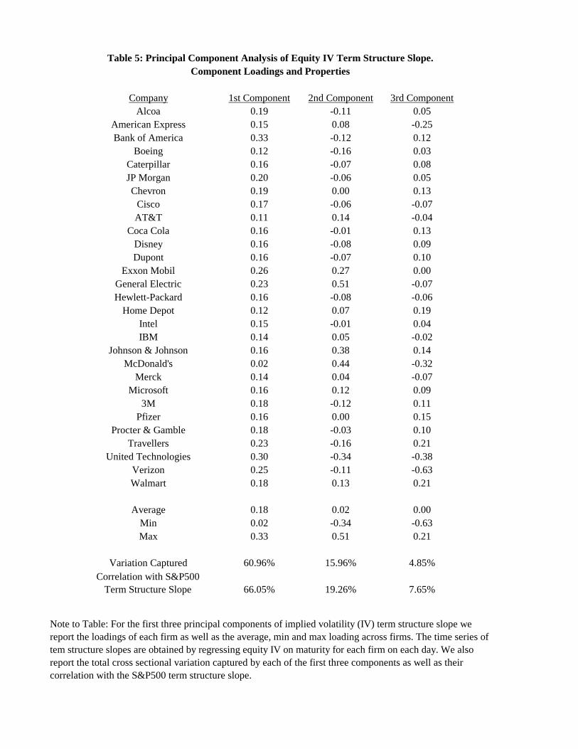
Company 1st Component 2nd Component 3rd Component

Alcoa 0.19 -0.11 0.05

American Express 0.15 0.08 -0.25

Bank of America 0.33 -0.12 0.12

Boeing 0.12 -0.16 0.03

Caterpillar 0.16 -0.07 0.08

JP Morgan 0.20 -0.06 0.05

Chevron 0.19 0.00 0.13

Cisco 0.17 -0.06 -0.07

AT&T 0.11 0.14 -0.04

Coca Cola 0.16 -0.01 0.13

Disney 0.16 -0.08 0.09

Dupont 0.16 -0.07 0.10

Exxon Mobil 0.26 0.27 0.00

General Electric 0.23 0.51 -0.07

Hewlett-Packard 0.16 -0.08 -0.06

Home Depot 0.12 0.07 0.19

Intel 0.15 -0.01 0.04

IBM 0.14 0.05 -0.02

Johnson & Johnson 0.16 0.38 0.14

McDonald's 0.02 0.44 -0.32

Merck 0.14 0.04 -0.07

Microsoft 0.16 0.12 0.09

3M 0.18 -0.12 0.11

Pfizer 0.16 0.00 0.15

Procter & Gamble 0.18 -0.03 0.10

Travellers 0.23 -0.16 0.21

United Technologies 0.30 -0.34 -0.38

Verizon 0.25 -0.11 -0.63

Walmart 0.18 0.13 0.21

Average 0.18 0.02 0.00

Min 0.02 -0.34 -0.63

Max 0.33 0.51 0.21

Variation Captured 60.96% 15.96% 4.85%

66.05% 19.26% 7.65%

Table 5: Principal Component Analysis of Equity IV Term Structure Slope.

Component Loadings and Properties

Note to Table: For the first three principal components of implied volatility (IV) term structure slope we

report the loadings of each firm as well as the average, min and max loading across firms. The time series of

tem structure slopes are obtained by regressing equity IV on maturity for each firm on each day. We also

report the total cross sectional variation captured by each of the first three components as well as their

correlation with the S&P500 term structure slope.

Correlation with S&P500

Term Structure Slope

Average Total

Ticker Kappa Theta Delta Rho Beta Spot Volatility

SPX 3.20 0.0403 0.508 -0.736 20.02%

AA 2.37 0.0293 0.373 -0.725 1.33 26.56%

AXP 0.81 0.0316 0.227 -0.781 1.13 22.59%

BAC 0.99 0.0204 0.202 -0.882 0.96 19.19%

BA 0.79 0.0462 0.270 -0.579 1.21 24.20%

CAT 3.07 0.0348 0.463 -0.645 1.06 21.16%

JPM 1.59 0.0247 0.280 -0.908 1.16 23.22%

CVX 2.65 0.0185 0.313 -0.729 0.85 17.03%

CSCO 0.71 0.0611 0.294 -0.930 1.15 23.05%

T 0.62 0.0656 0.286 -0.695 0.98 19.62%

KO 0.62 0.0219 0.165 -0.707 0.88 17.65%

DIS 0.85 0.0348 0.243 -0.762 1.12 22.43%

DD 3.25 0.0101 0.257 -0.832 1.12 22.49%

XOM 2.41 0.0129 0.249 -0.701 0.93 18.69%

GE 0.62 0.0332 0.203 -0.799 1.02 20.32%

HPQ 1.39 0.0534 0.386 -0.947 0.91 18.23%

HD 1.23 0.0133 0.180 -0.648 1.24 24.76%

INTC 1.39 0.0750 0.394 -0.975 1.17 23.35%

IBM 0.76 0.0175 0.163 -0.582 1.02 20.47%

JNJ 2.00 0.0164 0.256 -0.822 0.88 17.56%

MCD 2.47 0.0310 0.391 -0.623 1.04 20.73%

MRK 2.57 0.0424 0.467 -0.795 0.91 18.24%

MSFT 1.19 0.0996 0.486 -0.861 0.75 14.97%

MMM 1.96 0.0375 0.383 -0.775 0.87 17.38%

PFE 3.29 0.0286 0.434 -0.739 0.97 19.33%

PG 0.53 0.0505 0.231 -0.775 0.79 15.76%

TRV 2.50 0.0164 0.286 -0.759 1.17 23.46%

UTX 0.42 0.0376 0.177 -0.656 1.10 22.00%

VZ 1.00 0.0341 0.261 -0.935 1.13 22.71%

WMT 1.70 0.0165 0.237 -0.605 1.01 20.24%

Note to Table: We use option data from 2002 to 2005 to estimate risk-neutral

parameter values for the market index as well as the 29 individual equities. The

individual equity parameters are estimated taking the market index parameter

values as given. The last column report the average spot volatility through the

sample.

Table 6: Model Parameters and Properties

Average Average Absolute

Average Instantaneous Term-Structure

Ticker Beta Spot Volatility Skewness Slope

(ASV) (AISK) (AATS)

AA 1.33 0.33 -0.39 0.07

AXP 1.13 0.29 -0.33 0.07

BAC 0.96 0.22 -0.31 0.05

BA 1.21 0.30 -0.32 0.07

CAT 1.06 0.30 -0.34 0.04

JPM 1.16 0.34 -0.36 0.11

CVX 0.85 0.23 -0.28 0.03

CSCO 1.15 0.42 -0.32 0.09

T 0.98 0.30 -0.28 0.06

KO 0.88 0.21 -0.25 0.04

DIS 1.12 0.32 -0.29 0.07

DD 1.12 0.26 -0.36 0.05

XOM 0.93 0.24 -0.28 0.04

GE 1.02 0.27 -0.30 0.06

HPQ 0.91 0.39 -0.36 0.08

HD 1.24 0.32 -0.31 0.08

INTC 1.17 0.40 -0.40 0.11

IBM 1.02 0.28 -0.25 0.05

JNJ 0.88 0.22 -0.28 0.04

MCD 1.04 0.30 -0.31 0.06

MRK 0.91 0.26 -0.36 0.05

MSFT 0.75 0.30 -0.36 0.08

MMM 0.87 0.23 -0.31 0.05

PFE 0.97 0.28 -0.34 0.05

PG 0.79 0.19 -0.25 0.04

TRV 1.17 0.30 -0.35 0.07

UTX 1.10 0.27 -0.29 0.06

VZ 1.13 0.30 -0.36 0.08

WMT 1.01 0.25 -0.28 0.05

100% 57% -43% 55%

Table 7: In-Sample Correlations of Beta with Model Implied

Volatility Level, Skewness, and Term-Structure Slope.

Correlation with

Beta Estimates

Note to Table: We use the market index as well as the 29 individual equity parameter

estimated to compute the average of the model implied spot volatility (ASV - column 2),

instantaneous skewness (AISK - column 3), and absolute slope of the term-structure for

each firm (AATS - column 4). The correlation estimates represent the correlation of the

betas with the measure considered. We report the estimated betas in column 1 for

convenience. Note that all quantities are estimated over the 2002-2005 sample period.

Ticker IVRMSE Vega RMSE IVRMSE IV Bias IVRMSE IV Bias

SPX 0.91% 0.87% 0.98% 0.03% 0.82% 0.27%

AA 1.28% 1.28% 1.29% -0.36% 1.26% 0.57%

AXP 1.26% 1.26% 1.25% -0.50% 1.27% 0.61%

BAC 1.83% 1.83% 1.75% -1.18% 1.91% 1.40%

BA 1.41% 1.40% 1.33% -0.55% 1.49% 0.83%

CAT 1.32% 1.32% 1.23% -0.58% 1.44% 0.83%

JPM 2.21% 2.20% 2.07% -1.31% 2.35% 1.59%

CVX 1.45% 1.45% 1.32% -0.72% 1.61% 1.08%

CSCO 1.34% 1.34% 1.42% -0.02% 1.25% 0.14%

T 1.77% 1.77% 1.77% -1.13% 1.77% 1.02%

KO 1.20% 1.20% 1.17% -0.57% 1.23% 0.75%

DIS 1.30% 1.30% 1.30% -0.26% 1.31% 0.40%

DD 1.63% 1.63% 1.51% -0.78% 1.78% 1.15%

XOM 1.25% 1.25% 1.20% -0.65% 1.29% 0.69%

GE 1.50% 1.50% 1.39% -0.89% 1.60% 0.94%

HPQ 1.28% 1.28% 1.32% -0.11% 1.24% 0.17%

HD 1.28% 1.28% 1.26% -0.48% 1.30% 0.64%

INTC 1.41% 1.41% 1.45% -0.16% 1.37% 0.10%

IBM 1.47% 1.46% 1.45% -0.42% 1.50% 0.66%

JNJ 1.59% 1.59% 1.46% -0.83% 1.73% 1.08%

MCD 1.51% 1.51% 1.42% -0.49% 1.61% 0.70%

MRK 1.52% 1.52% 1.45% -0.88% 1.59% 1.08%

MSFT 1.80% 1.79% 1.94% -0.09% 1.63% 0.21%

MMM 1.56% 1.56% 1.44% -0.72% 1.69% 1.13%

PFE 1.29% 1.28% 1.21% -0.65% 1.37% 0.82%

PG 1.61% 1.61% 1.47% -0.65% 1.76% 0.95%

TRV 1.50% 1.50% 1.45% -0.63% 1.56% 0.83%

UTX 1.30% 1.30% 1.23% -0.48% 1.39% 0.83%

VZ 2.19% 2.20% 2.10% -1.30% 2.28% 1.56%

WMT 1.31% 1.32% 1.31% -0.43% 1.31% 0.51%

Table 8: Model Fit. Index and Equity Options

All Contracts OTM Calls OTM Puts

Note to Table: For the S&P500 index and for each firm we compute the implied volatility root mean

squared error (IVRMSE) along with the vega-based approximation used in estimation. We also report

IVRMSE as well as IV bias (market less model) for call and put options separately.