prices of state-contingent claims implicit in option prices€¦ · · 2011-10-31prices of...

Prices of State-Contingent Claims Implicit in Option PricesAuthor(s): Douglas T. Breeden and Robert H. LitzenbergerSource: The Journal of Business, Vol. 51, No. 4 (Oct., 1978), pp. 621-651Published by: The University of Chicago PressStable URL: http://www.jstor.org/stable/2352653Accessed: 29/08/2010 11:06

Your use of the JSTOR archive indicates your acceptance of JSTOR's Terms and Conditions of Use, available athttp://www.jstor.org/page/info/about/policies/terms.jsp. JSTOR's Terms and Conditions of Use provides, in part, that unlessyou have obtained prior permission, you may not download an entire issue of a journal or multiple copies of articles, and youmay use content in the JSTOR archive only for your personal, non-commercial use.

Please contact the publisher regarding any further use of this work. Publisher contact information may be obtained athttp://www.jstor.org/action/showPublisher?publisherCode=ucpress.

Each copy of any part of a JSTOR transmission must contain the same copyright notice that appears on the screen or printedpage of such transmission.

JSTOR is a not-for-profit service that helps scholars, researchers, and students discover, use, and build upon a wide range ofcontent in a trusted digital archive. We use information technology and tools to increase productivity and facilitate new formsof scholarship. For more information about JSTOR, please contact [email protected].

The University of Chicago Press is collaborating with JSTOR to digitize, preserve and extend access to TheJournal of Business.

http://www.jstor.org

http://www.jstor.org/action/showPublisher?publisherCode=ucpress

http://www.jstor.org/stable/2352653?origin=JSTOR-pdf

http://www.jstor.org/page/info/about/policies/terms.jsp

http://www.jstor.org/action/showPublisher?publisherCode=ucpress

Douglas T. Breeden University of Chicago

Robert H. Litzenberger Stanford University

Prices of State-contingent Claims Implicit in Option Prices*

the absence of a natural, agreed upon, and manageably small set of state defini- tions puts severe obstacles in the way of examining data about observable security behavior in terms of underlying choices for sequences of time state claims. [Hirshleifer 1970, p. 277]

While the state-preference approach is perhaps more general than the mean- variance approach and provides an elegant framework for investigating theoretical is- sues, it is unfortunately difficult to give it empirical content. [Jensen 1972, p. 357]

I. Introduction

The time-state preference approach to general equilibrium in an economy as developed by Arrow (1964) and Debreu (1959) is one of the most general frameworks available for the theory of finance under uncertainty. Given the prices of primitive securities (a security that pays $1.00 contingent upon a given state of the world at a given date, and zero otherwise, is a primitive

This paper implements the time-state preference model in a multiperiod economy, deriving the prices of primitive securities from the prices of call options on aggregate consumption. These prices permit an equilibrium valuation of assets with uncertain payoffs at many future dates. Furthermore, for any given portfolio, the price of a $1.00 claim received at a future date, if the portfolio's value is between two given levels at that time, is derived explicitly from a second partial derivative of its call- option pricing function. An intertemporal capital asset pricing model is derived for payoffs that are jointly lognormally distributed with aggregate consumption. It is shown that using the Black-Scholes equation for options on aggregate consumption implies that individuals' preferences aggregate to isoelastic utility.

(Journal of Business, 1978, vol. 51, no. 4) ? 1978 by The University of Chicago 0021-9398/78/5104-0005$02.21

621

* Research support for this paper was provided by the Stanford Program in Finance. The authors gratefully ac- knowledge helpful comments on earlier drafts by many of our colleagues in seminars and conversations, especially those of Sudipto Bhattacharya, Michael Brennan, Paul Cootner, John Cox, Jon Ingersoll, Merton Miller, Steve Ross, and Mark Rubinstein. Of course, the authors are solely responsible for any remaining errors.

622 Journal of Business

security), the value of any uncertain stream of cash flows is easily calculated. However, the two quotes above indicate that the application of the time-state preference model to practical problems in finance, such as capital budgeting, is not at all immediate. This paper may be viewed as an attempt to make the state preference model operational in a multiperiod economy by deriving the prices of primitive securities from the prices of European call options on aggregate-consumption expenditures at each date.

The papers of Wilson (1970), Schrems (1973), Friesen (1974), and Ross (1976) have shown in a single-period context that the vector space of contingent claims on a given portfolio is spanned by options on that portfolio with various exercise prices. In Section II, the price of a security paying $1.00 in T periods if the value of a given portfolio (e.g., the market) is MT at that time, and zero otherwise, is derived from the prices of European call options on the portfolio with various exercise prices and with T periods to maturity.' If the portfolio's value in T periods has a continuous probability distribution, then the price of such an "elementary claim" on the given portfolio is determined by the second partial derivative (assuming it exists) of the European call- option pricing function for the portfolio with respect to the exercise price, evaluated at an exercise price of MT. From these elementary- claim prices, the value of any asset whose payoffs are known functions of the portfolio's values at future dates (derivative assets) is derived.

As an example, the call-option pricing equation of Black and Scholes (1973) is used in Section III to derive the value of a security that pays $1.00 if the given portfolio is between two stated levels in T periods, for example, if the market portfolio in 1 year is between 10% and 20% higher than its current level. The prices of these "delta securities" for a plausible set of parameters are presented in tables 2 and 3. Delta- security prices may be used to determine the prices of "complex options and corporate liabilities" given in Black's (1974) note, and they may be used to find values for Hakansson's (1977) "supershares," as given in Garman (1976). However, unlike Black's and Garman's pricing equations, the methods of this paper do not depend upon the continuous-time model of prices as diffusion processes, nor upon the Black-Scholes option-pricing equation.

An alternative set of estimates of delta-security prices for the market portfolio (corresponding to tables 2 and 3) is given by Banz and Miller (1978). They use the Black-Scholes model in a sequential manner to estimate call-option prices on the market portfolio when the interest rate is stochastic. Of course, as noted in Section III, the Black-Scholes equation is consistent with a stochastic interest rate for certain prefer-

1. The analysis is quite general in that the price of an elementary contingent claim on any portfolio may be determined from the appropriate call options on that portfolio.

State-contingent Claims in Option Prices 623

ence and/or probabilistic assumptions, eliminating the need for a sequential approach in those cases. In general, however, option pricing with a stochastic interest rate remains an unsolved problem, and the Banz-Miller estimates may approximate this unknown solution. From an equilibrium-valuation standpoint, their estimates may only be used to value derivative assets of the market portfolio since, with a stochastic interest rate, there exist random returns that have zero expectations, conditional upon various market levels, that have positive prices. This fact may be seen from Section V or from Merton's (1973a) analysis of hedging against opportunity set changes in an intertemporal model.

Anticipating the proof in Section V that the prices of elementary claims on aggregate consumption (or, in one case, the market portfolio) are essential to the pricing of all securities, Section IV presents a comparative statics analysis of the elementary-claim pricing function. In the context of the Black-Scholes option equation, changes in the market's dividend yield, current value, and variance rates are shown to affect elementary-claim prices in economically explicable directions. The structures of elementary-claims prices with respect to their times to maturity and with respect to their values upon which payment is contingent are also examined in Section IV.

In Section V, it is proven that if individuals have time-additive and state-independent lifetime utility functions for consumption expenditures, and, conditional upon each potential level of aggregate consumption, all agree upon the probabilities of states of the world, then each individual's optimal consumption at each date may be expressed as a function of (only) aggregate consumption at that date. Thus it is shown that any Pareto-optimal allocation of time-state-contingent claims to consumption among individuals can be attained by a securities market consisting only of European call options on aggregate consumption at each date. It is then shown that the prices of primitive securities may be expressed in terms of the prices of elementary claims on aggregate consumption, which may be obtained from prices of call options on aggregate consumption by the method of Section II. From this derivation of primitive-security prices, a valuation equation is obtained for all existing securities and capital-budgeting projects in terms of the prices of European call options on aggregate consumption. It is shown that knowledge of an asset's entire pattern of time-state-contingent payoffs is not required for valuation; only the expected payoffs on the asset, conditional upon aggregate consumption at each date, are required by the valuation equation.

The portfolio result of Section V is the appropriate multiperiod generalization of a similar single-period result obtained by Mossin (1973) and Hakansson (1977). Their single-period result that each individual' s optimal state-contingent wealth is a function of only aggregate


wealth is seen to be nonoptimal in a general multiperiod economy. However, if it is further assumed that there exists a one-to-one correspondence between aggregate real consumption and aggregate real wealth (the market portfolio),2 then European call options on the market portfolio maturing at each future date may effect any Pareto- optimal allocation of time-state-contingent claims to consumption. In this case, with the assumptions required for the option-pricing theory of Black and Scholes (1973) and its extensions by Merton (1973b), the prices of primitive securities may be derived in terms of market data that are known or may be estimated and in terms of the probability distribution of states. However, the required one-to-one' mapping of aggregate consumption onto aggregate wealth will exist only for specific preference assumptions, for example, logarithmic utility functions. Therefore, the prices of primitive securities determined from the prices of options on aggregate consumption are of considerably greater generality, as this derivation requires much weaker restrictions on individuals' preferences.

In Section VI, assuming that the Black-Scholes equation correctly prices options on aggregate consumption, equilibrium values are determined for the class of assets with payoffs that are jointly lognormally distributed with aggregate consumption at a future date. These assets are shown to be appropriately priced in a multiperiod context by a capital asset pricing model similar to that derived by Sharpe (1964) and Lintner (1965) in a single-period economy.3 However, the relevant "beta" of an asset's payoff that is necessary for pricing should be measured with respect to aggregate consumption, rather than with respect to the market portfolio.4 Implications of this result for capital budgeting are discussed in Section VIII.

Section VII demonstrates that probabilistic assumptions about the pricing process for claims on consumption cannot be made independently of preference assumptions. Specifically, under certain assumptions, it is shown that the Black-Scholes formula prices options on aggregate consumption correctly if and only if individuals' prefer-

2. This paper deals with a single-good model which could be extended to the multi- good case if all individuals have the same price index. The existence of a price index that is independent of an individual's wealth requires that all income elasticities of demand be unitary. (See Grauer and Litzenberger [1974] for a discussion of valuation in a multicommodity world.) For the single-good case of this paper, since individuals will be assumed to have preferences that are state independent in terms of the good, consumption and wealth should be thought of as real magnitudes.

3. As this multiperiod model may have stochastic investment opportunities, it is entirely consistent with Merton's (1973a) "multifactor" intertemporal capital asset pricing model (CAPM).

4. The beta of a security with respect to aggregate consumption is equal to its payoff's covariance at time t with aggregate consumption at time t, divided by the variance of aggregate consumption at time t.


ences aggregate to a function displaying constant relative risk aversion (CRRA).5

Finally, Section VIII summarizes the major results of the paper and emphasizes their implications for capital budgeting.

II. Pricing Elementary Contingent Claims from Option Prices

An "elementary claim" on any security or portfolio of securities is defined here as a security that pays $1.00 at a given date, that is, in T periods, if the value of the portfolio is M at that time; if the value of the portfolio is not M in T periods, the elementary claim expires paying nothing. This section derives the price, P(M, T), of such an elementary contingent claim in terms of the prices of European call options on the underlying portfolio. The elementary claim may be created by long and short positions in call options having various exercise prices, each with a time to maturity of T; the price of the elementary claim must then be the cost of the portfolio of calls that gives the desired payoff. Under certain assumptions, it is shown in Section V that only the values of such elementary claims on aggregate consumption, that is, $1.00 if aggregate consumption is C in T periods, are essential to the pricing of primitive securities in the state preference model of Arrow and Debreu. For the special case where there exists a one-to-one mapping between aggregate consumption at a given time and the level of the market portfolio at that time, the price on an elementary claim on aggregate consumption will equal the price of an elementary claim on the corresponding level of the market portfolio. For this reason, the analysis will proceed with the underlying security being denoted as "the market" or as "aggregate wealth," although the method of pricing of this section is valid for claims on any security or portfolio. Throughout this paper, it is assumed that there are no restrictions on short sales, that there are no transactions costs or taxes, and that investors may borrow at the riskless rates of interest.

Initially, suppose that the value of the market portfolio in T periods has a discrete probability distribution with possible values of: M = $1.00, $2.00, . . . , $N. Denote the vector of payoffs of a European call option on the market with T periods to maturity and with an exercise price of X as c(X, T); its price will be denoted by c(X, T). For calls with exercise prices of $0, $1.00, and $2.00, the state-contingent payoffs at T, c(X, T) are as shown in table 1.

Note that as the exercise price of a call option is increased from X to

5. In a later paper, derived independently of this paper, Brennan (1977) proves the same theorem with respect to wealth by assuming that aggregate consumption follows a random walk. He also shows that normality implies an assumption of constant absolute risk aversion.


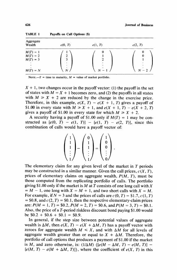
TABLE 1 Payoffs on Call Options ($)

Aggregate Wealth c(0, T) c(1, T) c(2, T)

M(T)=1 / 1 0 0 M(T) = 2 2 1 0 M(T) = 3 t 3 S t( 2 (12)

M(T) = N N N- I N-2

NOTE.-T = time to maturity, M = value of market portfolio.

X + 1, two changes occur in the payoff vector: (1) the payoff in the set of states with M = X + 1 becomes zero, and (2) the payoffs in all states with M : X + 2 are reduced by the change in the exercise price. Therefore, in this example, c(X, T) - c(X + 1, T) gives a payoff of $1.00 in every state with M : X + 1, and c(X + 1, T) - c(X + 2, T) gives a payoff of $1.00 in every state for which M ? X + 2.

A security having a payoff of $1.00 only if M(T) = 1 may be constructed as [c(0, T) - c(l, T)] - [c(l, T) - c(2, T)], since this combination of calls would have a payoff vector of:

1'-1?~~ 1)

The elementary claim for any given level of the market in T periods may be constructed in a similar manner. Given the call prices, c (X, T), prices of elementary claims on aggregate wealth, P(M, T), must be those computed from the replicating portfolio of calls. The portfolio giving $1.00 only if the market is M at T consists of one long call with X = M - 1, one long with X = M + 1, and two short calls with X = M. For example, if N = 3 and the prices of calls are c (0, T) = $1.7, c (1, T) = $0.8, and c (2, T) = $0. 1, then the respective elementary-claim prices are: P(M = 1, T) = $0.2, P(M = 2, T) = $0.6, andP(M = 3, T) = $0.1. Also, the price of a T-period riskless discount bond paying $1.00 would be $0.2 + $0.6 + $0.1 = $0.9.

In general, if the step size between potential values of aggregate wealth is AM, then c(X, T) - c(X + AM, T) has a payoff vector with zeroes for aggregate wealth M - X, and with AM for all levels of aggregate wealth greater than or equal to X + AM. Therefore, the portfolio of call options that produces a payment of $1.00 if the market is M, and zero otherwise, is: (1/AM) {[c(M - AM, T) - c(M, T)] - [c(M, T) - c(M + AM, T)]}, where the coefficient of c(X, T) in this


expression is the number of calls with exercise price of X and time to maturity of T that should be held in the portfolio.

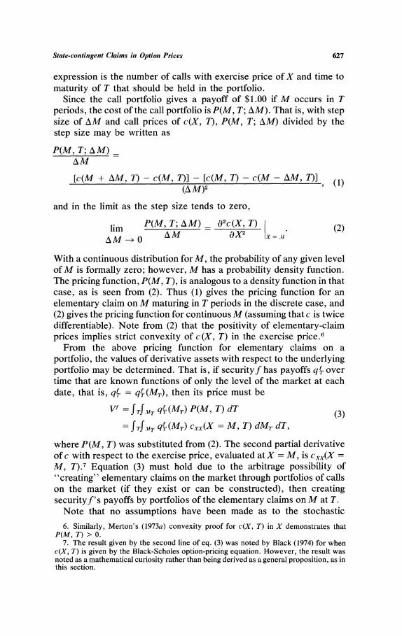
Since the call portfolio gives a payoff of $1.00 if M occurs in T periods, the cost of the call portfolio is P(M, T; AM). That is, with step size of AM and call prices of c(X, T), P(M, T; AM) divided by the step size may be written as

P(M, T; AM) -

AM

[c(M + AM, T) - c(M, T)] - [c(M, T) - c(M - AM, T)] (AM)2 , (1)

and in the limit as the step size tends to zero,

lim P(M, T; AM) a2c(X, T) AMM->0 AM Ix2 (x=2)

With a continuous distribution for M, the probability of any given level of M is formally zero; however, M has a probability density function. The pricing function, P(M, T), is analogous to a density function in that case, as is seen from (2). Thus (1) gives the pricing function for an elementary claim on M maturing in T periods in the discrete case, and (2) gives the pricing function for continuous M (assuming that c is twice differentiable). Note from (2) that the positivity of elementary-claim prices implies strict convexity of c (X, T) in the exercise price.

From the above pricing function for elementary claims on a portfolio, the values of derivative assets with respect to the underlying portfolio may be determined. That is, if security has payoffs qf over time that are known functions of only the level of the market at each date, that is, qf = qf (MT), then its price must be

= I Tf qf (MT) P(M, T) dT

= I TfMT qf (MT) cxx(X = M, T) dMT dT,

where P(M, T) was substituted from (2). The second partial derivative of c with respect to the exercise price, evaluated at X = M, is cxx(X =

M, T).9 Equation (3) must hold due to the arbitrage possibility of "creating" elementary claims on the market through portfolios of calls on the market (if they exist or can be constructed), then creating securityf's payoffs by portfolios of the elementary claims on M at T.

Note that no assumptions have been made as to the stochastic 6. Similarly, Merton's (1973a) convexity proof for c(X, T) in X demonstrates that

P(M, T) > 0. 7. The result given by the second line of eq. (3) was noted by Black (1974) for when

c(X, T) is given by the Black-Scholes option-pricing equation. However, the result was noted as a mathematical curiosity rather than being derived as a general proposition, as in this section.


process governing the movement of the underlying security's price or of the option's price. Aside from the perfect-markets assumption, the only requirement is that c(X, T) be twice differentiable for (3); even this differentiability assumption is not necessary for the discrete valuation equation obtainable from (1). Individuals' preferences and beliefs have not been restricted, as they will be reflected in the call-option prices.

There may be many different states of the world with the same level of aggregate consumption or aggregate wealth. For example, the distribution of total output among firms may vary over a group of states with the same level of aggregate output. Also, the state description at any date may include the history of events prior to that date. Thus there may be many interesting securities and capital-budgeting projects that are not proper derivative securities and whose values may not be determined by the valuation equation (3). It is shown in Section V that if, conditional upon any given level of aggregate consumption at time T, individuals agree upon the probabilities of states, if they have time- additive and state-independent utility functions for consumption, and if there is a correspondence between aggregate consumption and aggregate wealth, the same valuation formula (3) is obtained for all assets, with cash flows in the formula replaced by their expected values conditional upon the level of the market, E(qf I MT). When the first two of these conditions are met, but there is not a one-to-one mapping between aggregate consumption and aggregate wealth, Section V derives a general valuation equation similar to (3) in terms of prices of elementary claims on aggregate consumption and expected payoffs conditional upon levels of aggregate consumption. In that more general case,8 it is not appropriate to value all assets by using (3) with qT(MT)

being replaced by securities' expected payoffs, conditional upon the various levels of the market portfolio.9

III. An Example of Valuation Using the Black-Scholes Equation

An explicit formula for the value of a European call option, c (X, T), in a continuous-time economy when the underlying asset follows a diffusion process has been obtained by Black and Scholes (1973) and generalized by Merton (1973b). Also in a continuous-time economy, Cox and Ross (1975) and Merton (1976) obtained explicit valuation formulae for a European call option when the underlying asset's price follows a jump process. The Black-Scholes option-pricing formula has been derived in a discrete-time economy for individuals whose utility functions

8. The conditions for a one-to-one mapping are quite stringent, e.g., logarithmic utility.

9. This fact considerably restricts the classes of assets and capital-budgeting projects for which the Banz-Miller valuation results are valid.


are isoelastic (CRRA) by Rubinstein (1976). For their respective economies, each of these formulae may be used to evaluate cXx and, hence, the prices of elementary contingent claims on the underlying asset, P(M, T).

In this section and the next, prices of elementary claims on a portfolio are examined under conditions that permit the derivation of the Black-Scholes call-option pricing equation as generalized by Mer- ton. That equation is

c(X, T) = Moe-8T N(dl) -B(T) X N(d2), (4)

where

2 - --~~~~~~~~~~

and d, = d2 + O-T\I; rT = -{In [B(T)]}IT is the (continuously com- pounded) yield to maturity available on T-period riskless bonds and -T- is the average variance rate for (In M), that is, o-r = var (In MT)IT; MO is the current value of the optioned portfolio and 5 is the portfolio's continuously paid dividend yield.10 The standard normal cumulative distribution function is N(d), which is tabulated.

The European call-option pricing function given by (4) is the same as the original Black-Scholes solution when there are no dividends, 5 = 0, when the term structure is flat, B(T) = e-rT, and when the variance of (In M) is proportional to time, o- 2 = o-2. Merton generalized the Black- Scholes solution to the case of a proportional dividend rate and to a particular stochastic process for interest rates. To incorporate the latter generalization, OT in (4) should be interpreted as oT- T =fT (0 +

7B2- 2PIBo-ImoB) dt, where o-B is the variance rate on the discount bond maturing at T. Also, the Black-Scholes equation correctly values options on aggregate consumption, even with a fairly general form of stochastic interest rates, if it is assumed that individuals' preferences aggregate to a utility function displaying CRRA and if consumption is lognormally distributed at each future date." While the CRRA assumption is quite strong, it is shown in Section VI to be a necessary condition for pricing options on aggregate consumption via the Black- Scholes formula. The importance of pricing options on aggregate consumption will be shown in Section V. However, at this point we return to the simpler task of pricing elementary claims on any portfolio when the Black-Scholes equation is just assumed to correctly value options

10. With discrete proportional dividends paid n times between now and T, e-8T would be replaced by (1 - 8)n and the analysis would be unchanged. See Geske (1976) for a CRRA treatment of stochastic dividend yield.

11. In this model aggregate consumption may follow a discontinuous stochastic process.


on that portfolio. Again, the market portfolio is used for illustrative purposes.

By differentiating the call-option pricing function, (4), twice with respect to the exercise price and evaluating the resulting function at X = M, the price of $1.00 contingent upon aggregate wealth being M in T periods (scaled up by dividing by dM) is found from (2) and (4):

dMT MT O CT\ / n[d2(X = MT)] (5)

where n(d) is the standard normal probability density function n(d) =

(2,)-1/2e-d212.12

By substituting (5) into (3), the valuation equation for all assets with cash flows that are known functions of the market level and time (derivative assets) is obtained. The needed parameters for valuation are the cash flows of the security over time, conditional upon the level of the market, the market's dividend yield, and its variance of rate of return, which may be estimated. The term structure of interest rates is observable. As the analysis of Section II and the present section is valid for derivative securities of any security or portfolio that meets the Black-Scholes assumptions, the valuation equation from (5) and (3) may be quite useful. A numerical example of the general method of pricing elementary claims and derivative assets of a portfolio follows, using the Black-Scholes call-option pricing equation for c(X, T).

Consider a security that pays $1.00 at t* if aggregate wealth at t* is greater than or equal to a prespecified level Y and zero otherwise. The time to maturity of this security is T t* - t. Let the value of this security be G(Y, T), the cumulative of the pricing function (from the right), since G(Y, T) = fy P(M, T), which is from (5):

G(Y, T) = K B(T) n[d2(X = Mt*)] dMt* jy Mt *0uVT (6)

= B(T)N[d2(X = Y)

where the solution given in the second line was obtained by changing variables from Mt* to d2 by the following relation:

Mt* =Moexp[(r-, - '2 ) T-d2&vIr1

with JacobianJ= -Moo-V7 exp [(r - 8 T - d2o I 13

For a time period of 1 year, T = 1, the values of G(Y, T) were

12. By a transformation of variables from MT to d2, it is seen that P(M, T)Idd2 =

B(T)n(d2), which is the price of a discount bond times the risk-neutral density of Cox and Ross (1976).

13. Note that for Yt = 0, the cumulative pricing function gives the price of a riskless discount bond with t periods to maturity, since receipt of $1.00 is certain.


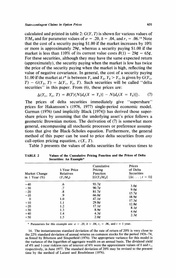
calculated and printed in table 2: G(Y, T) is shown for various values of Y/Mo and for parameter values of C = .20, 8 = .04, and r, = .06.14 Note that the cost of a security paying $1.00 if the market increases by 10% or more is approximately 29?, whereas a security paying $1.00 if the market is less than 110% of its current value costs B(1) - 29? = 65?. For these securities, although they may have the same expected return (approximately), the security paying when the market is low has twice the price of the security paying when the market is high, reflecting the value of negative covariance. In general, the cost of a security paying $1.00 if the market at t* is between Y1 and Y2, Y2 > Y1, is given by G(Y1, T) - G(Y2, T) = A(Y1, Y2, T). Such securities will be called "delta securities" in this paper. From (6), these prices are:

A (Y1, Y2, T) = B(T){N[d2(X = Y})] - N[d2(X = Y2)]}. (7)

The prices of delta securities immediately give "supershare" prices for Hakansson's (1976, 1977) single-period economic model. Garman (1976) (and implicitly Black [1974]) has derived those supershare prices by assuming that the underlying asset's price follows a geometric Brownian motion. The derivation of (7) is somewhat more general, encompassing all stochastic processes or preference assumptions that give the Black-Scholes equation. Furthermore, the general method of this paper can be used to price delta securities from any call-option pricing equation, c(X, T).

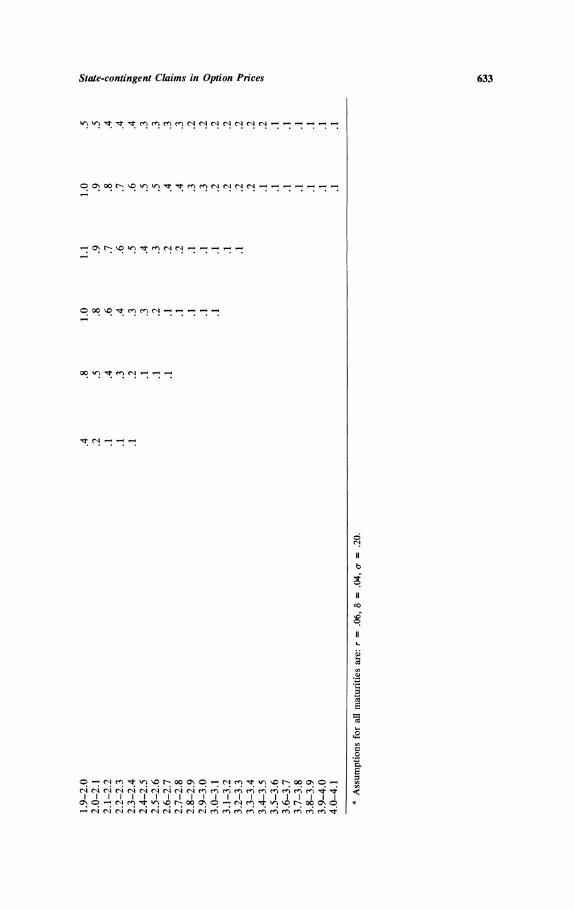
Table 3 presents the values of delta securities for various times to

TABLE 2 Values of the Cumulative Pricing Function and the Prices of Delta Securities: An Example*

Cumulative Prices 1-Year Price Pricing of Delta

Market Change Relatives Function Securities in 1 Year (%) (Y11Mo) [G(Y11M0)] ... .; t = 1)]

-40 .6 93.70 3.0 -30 .7 90.70 9.00 -20 .8 81.70 15.70 -10 .9 66.0? 18.90

0 1.0 47.10 17.30 +10 1.1 29.80 12.80 +20 1.2 17.10 8.1? +30 1.3 8.90 4.60 +40 1.4 4.30 2430 +50 1.5 2.0?

* Parameters for this example are: a- .20, 8 = .04, r, = .06, and t = 1 year.

14. The instantaneous standard deviation of the rate of return of 20% is very close to the 22% standard deviation of annual returns on common stocks for the period 1926-74, as found by Ibbotson and Sinquefield (1976). The appropriate variance for this model is the variance of the logarithm of aggregate wealth on an annual basis. The dividend yield of 4% and 1-year riskless rate of interest of 6% were the approximate values of 8 and r1, respectively, in June 1977. The standard deviation of 20% may be revised to the present time by the method of Latan6 and Rendelman (1976).


C- \ "C \ C) o o t- "C , t m C' o) CN CN r c c

~~~~~~~~CN CIW -

N CI" '"t

~~~~~~~~W N ,t It 11 W) 00 C'I r', M

m~~~~~Ci- 1, 06 06 t-t- r-: 16 W; - e; cl C-i

0 00 e'i '--e' e;i W~06r- ci 6-4 -

;^ ; v C O 00 00 O m N W C004

0

C) C-4 mt WC " ON - O N bC - t W N C 0 C

Ev~~~~ . . . . .............14 4

> v ~O ONbO ef00 ? ' 1

C1N ?C ON 000 N

o~~~~ N ~C- ~N e-

*;

0

'0 t N

ON N

I o 'fN 00 ?boo ; - '1o} PN 0 toNo4

- l l l l l l l l < 00 o N ^t f bo ooN 00 bo


W) W) "t "t "t M M M M C1 C1 CT CT CT CT C

o O\ 00 N "C e' ' e e" " - I I

t - O, N <, e' e'

0)00 IC ,I, C-

Ci

b

Cd

04

I I i

I l I I

Ii I~ Ii Ii Ii el el el el el el el el I

l I

. *


maturity ranging from 3 months to 5 years, using the same parameters as in table 2. Note that the number of rows in this price matrix can be as great or as small as desired since equation (7) is quite general. As a practical matter, the number of rows chosen should depend upon the range and variability of the uncertain cash flows to be valued.t5 The value of assetf with payoff qf(Yi, Yi+1, T) when the underlying portfolio is between Yi and Yi+ in T periods is

Vf = YTZiA(Yi, Yi+, T)qf(Yi, Yi+l, T). (8)

Equivalently, arranging the asset's contingent payoffs in a matrix of the form of table 3, the asset's value is the box product of its payoff matrix with the matrix of delta prices. This technique has implications for capital-budgeting decisions that are discussed in Section VIII. Of course, as the underlying asset's price changes, or as other parameters change, the delta price matrix will change, causing corresponding changes in the values of derivative assets. An example of this effect is given by Banz and Miller (1978).

IV. Properties of Elementary Contingent-Claim Prices

The pricing function for $1.00 contingent upon a given level of the market in T periods, P(M, T), as given by equation (5), is the subject of the analysis of this section.t6 In particular, the elasticities of the pricing function with respect to its parameters are determined and interpreted. Note that, since the price of a riskless discount bond is an argument of P(M, T) andf MTP(M, T) = B(T), the partial derivatives of P(M, T) with respect to its other arguments must increase P(M, T) at some levels of MT and decrease P(M, T) at other levels of MT, since the sum over MT

remains constant. As the initial level of the market, MO, is increased, ceteris paribus,

the probability distribution for future levels of the market is shifted upward. The increased probabilities of "high" levels of MT and the decreased probabilities of "low" levels of MT increase and decrease, respectively, their contingent-claim prices given by P(M, T). This is stated by the elasticity

O ln P(M, T) _ d2 (9) ln MO (9)'

where

d2 - l(MTn ) (rT 2 )

15. If qf is a continuous function of the portfolio value, rather than a step function as in (8), then Vf is given by the direct integration in (3).

16. The analysis of this section anticipates the utility implications of some of the results of Sections V and VI.


assuming 0-2 is constant. To verify that an increase in MO increases prices at high levels of MT and decreases P(M, T) for low levels of MT, note that d2 approaches -Xo as MT approaches +00 and d2 approaches +oo as MT approaches 0.

The elasticity of the pricing function with respect to the instantaneous standard deviation of the rate of growth of aggregate wealth is

Ol in P = d1d2 -1, (10) OIn o-

where d, = d2 + o-NV/T. This elasticity will be positive for very large and very small levels of MT and will be negative for MT near the center of its distributions This is explained by the fact that an increase in variance increases the probability of extreme observations relative to the probability of central observations.

The elasticity of P(M, T) with respect to the price of a T-period riskless discount bond, B(T), is:

lnB(T) o-V(T Therefore, an increase in B(T) lowers the prices of claims that pay when MT is very high and raises the prices of claims that pay when MT is very low. Since B(T) is such that B(T) = f MTP(M, T), the increase in B(T) must increase the sum of all claim prices maturing in T periods.

The price of a T-period discount bond in equilibrium is equal to each individual's ratio of expected marginal utility of consumption in T periods to his current marginal utility of consumption. Thus, an increase in B(T) may be associated with a diminished growth rate for consumption, which would decrease the probabilities (and prices of elementary claims) of high levels of the market in T periods. Alterna- tively, holding the expected growth rate of the market constant while decreasing the T-period riskless interest rate would indicate an increase in risk aversion as measured by individuals' utility functions for consumption in T periods. This would also explain the described effects of a change in B(T) on elementary-claim prices.

As the dividend rate is increased, the distribution of the level of the market at time T is shifted downward, ceteris paribus; corre- spondingly, the prices of securities that pay when MT is low are increased by an increase in the dividend rate, whereas the prices of securities that pay when MT is high are reduced. Mathematically,

a In P _ DeT (12)

which supports the preceding interpretation.

17. Since the mean of the distribution of MT is not a parameter for P(M, T), the phrase "near the center of its distribution" is used loosely; those levels of M for which Iln(MO/MT) I is not much larger than I (r - 8 - o-212)T I will be denoted as near the center of M's distribution.


The previous analyses have considered comparative statics changes in elementary-security prices due to changes in the parameters of P(M, T). These served to illustrate the functional form of the elementary- claim pricing equation. Now, consider the structure of elementary- security prices at a given point in time for various levels of the arguments of P(M, T), namely, the time to maturity, T, and the level of the market at maturity upon which payment is contingent, MT. These will be denoted the "maturity structure" and the "market-value structure" of elementary-security prices, respectively. Observe that the maturity structure is defined for a given market value (payoff level) M, and the market-value structure is defined for a given maturity T. In table 3 of the previous section, the maturity structure reflects movement across a row and the market-value structure is given by movement down a column.

As the level of the market upon which the claim is contingent increases, there are two essential effects on the price of the claim, P(M, T): (1) the probability of the payoff being received may increase or decrease, thereby increasing or decreasing, respectively, the claim price, and (2) the increased wealth of the economy in the payoff states will decrease the marginal utility of wealth, thereby decreasing the claim price. The elasticity of the claim price with respect to the level of the market that it is contingent upon (its exercise price) is

O InMT 1. (13)

For very low levels of MT (relative to its initial level), the elasticity will be positive due to the increasing probability of payoff as MT increases from a very improbable low level. For wealth levels of MT that are large, the elasticity of P with respect to MT will be negative due to the effects of both diminishing probability of payoff and of diminishing marginal utility.

The logarithm of P is concave in the logarithm of MT as

O2In P I <KO. (14) a(ln MT)2 T2 T

To verify the statement that, for a given probability of occurrence, as aggregate wealth in the payoff state increases the price of the state- contingent claim decreases due to the effects of diminishing marginal utility, assume that aggregate wealth follows a geometric Brownian motion and consider the following. Under this assumption, the ratio of P(M, T) to the probability of MT at T, IT(M, T) is18

18. With geometric Brownian motion for MT, the probability of MT at T, given MO, is

vr(M, T) = (27roT exp |- 1 [in (M - (a - a - 2/2)T1 . MT MO 2nd e M5).

Eq. (15) follows from this fact and eq. (5).


Pr(M, T) -B(T) exp a -t r In MO

T(a-r)(a + r-2-- 2-) (15)

where a is the expected total return on the market. Thus, the elasticity of the ratio of price to probability with respect to MT is

O In [P(M, T)/IT(M, T)] - _ --r < ? (16) OIn MT . (16

This proves the statement that, holding probabilities of MT at T constant, the prices of elementary claims on the market are a decreasing function of aggregate wealth.t9 As will be argued in Section VI, the fact that the right-hand side of (16) is independent of MT implies that use of the Black-Scholes option equation for pricing options on consumption requires an implicit assumption of preferences that aggregate to a function that exhibits constant relative risk aversion.

By examining the partial of P(M, T) with respect to the time to maturity, T, the maturity structure of elementary claim prices is obtained. Since B(T) = f MT P(M, T) = e-rTT is decreasing in T if all interest rates implicit in the term structure are positive, the sum of the claim prices must decrease as the time to maturity increases. However, the effects of a changing probability of the given level of M at T as T changes are evident in the following:

8In P = -r - 1 - - (r8 2 2 (17) OT ~27' /I 2~ 29

assuming that r is constant over time. The first term in (17) reflects the time effect on the value of $1.00. If

(r - 8 - o-2/2) is positive, then payoff levels of MT that are lower than the current level of the market MO will decrease in value with an increased time to maturity due to their diminished probabilities of occurrence. For payoff levels of aggregate wealth that are extremely high or low relative to the current level, the d2 term dominates (17), increasing the prices of payoffs at both extremes. This effect is due to the increased variance of aggregate wealth as time to maturity is increased, thus increasing the probabilities of extreme observations relative to the probabilities of more central observations.

V. Primitive Security Pricing in a Multiperiod Economy

In this section, the prices of primitive securities (each paying $1.00 contingent upon a given state at a given date) in a general multiperiod

19. In (16) it is assumed that (a - r)/o-2 > 0, which will be true if the return on the market portfolio is positively correlated with aggregate consumption. See Section VI for more explanation in terms of the CAPM. For options on aggregate consumption P(C, T)I vr(C, T) is shown in Section V to be proportional to social marginal utility.


state preference model are derived from the prices of call options on aggregate consumption maturing at each point in time, with exercise prices equal to the various possible levels of aggregate consumption at those points in time. Given these primitive-security prices, the prices of all assets may be calculated from their state-contingent payoffs. In fact, it will be shown that each security price may be determined from its expected payoffs, conditional upon aggregate consumption, and the prices of call options on aggregate consumption.

The economic model is of a multiperiod exchange economy with a single "real" good; there are F productive units (firms) in the economy whose output decisions are taken as predetermined. Contingent upon the occurrence of time-state ts, defined here as the occurrence of state s at time t, where s E St, the output of unit f is qf5 units of the consumption good. There are K consumers, each of whose preferences for state-contingent consumption allocations, {Ctk}, are assumed to be representable by the expected value of a von Neumann-Morgenstern utility function of the following form:20

Uk(ck, ci1, . . * , Ct%) = Xt~seSt 7TkUk(Ck), (18)

where u () is assumed to be monotonically increasing and strictly concave for each t. Individual k's subjective probability assessment for the occurrence of state s at time t is 7Tk , and Ctk is his consumption in period t if state s occurs. Note that individuals' preferences for lifetime consumption are assumed to be time additive and state independent, in that their utilities at t depend only on the amounts of the good con- sumed at that time, not on the state of the world or past or future consumption levels. It is assumed that all individuals have an infinite lifetime in (18), but their respective utilities for consumption may depend quite generally on time, that is, u(Ctk) = u(Ct, t).

Debreu (1959) has shown that there is a correspondence between Pareto-optimal allocations of contingent claims on consumption over dates and states among individuals and the allocations achieved by a competitive equilibrium with complete markets. Thus the equilibrium prices of securities in any competitive capital market that attains the same allocation of time-state-contingent claims on consumption as a complete market may be examined by analyzing the Lagrange multi- pliers (shadow prices for primitive securities for each time and state) of the corresponding Pareto-optimal allocation.2t In the following theorem and corollary, it is proven that a securities market consisting only of options on aggregate consumption at each date is sufficient for

20. For a model with continuous time and states, the summations in (18) would be integrals. A countably infinite number of states is permissible in a state preference model.

21. Debreu (1959) showed the correspondence between Pareto-optimal allocations and those of a competitive equilibrium with complete markets. See Nielsen (1974) for a discussion of the relation between pricing in Pareto-optimal capital markets and pricing in complete markets.


the attainment of an unconstrained Pareto optimum, given the following two assumptions: (Al) each individual has a time-additive, state- independent utility function for time-state contingent consumption allocations, and (A2) all individuals agree on the probabilities of states, conditional upon the level of aggregate consumption at the time.22 Therefore, individuals may disagree about the entire probability distribution for aggregate consumption at each date, but they must agree on the conditional probability distribution for states, for each given level of aggregate consumption. Mathematically, A2 implies that irks =

iTrcirtsic, where tk is individual k's probability for aggregate consumption being C at time t, and rtslc is his probability that state s occurs at time t, conditional upon consumption C at t.

Theorem 1. Intertemporal diversification: If (Al) each individual has a time-additive, state-independent utility function for lifetime consumption and (A2) all individuals agree upon the probabilities of states at any given date, conditional upon aggregate consumption at that date, then any unconstrained Pareto-optimal allocation of time-state- contingent consumption claims is such that, at each date, all states with the same level of aggregate consumption supplies have the same allocation. Furthermore, given (Al), (A2) is both necessary and sufficient for the theorem.23

An immediate corollary to theorem 1 is the following:

Corollary. Pareto-optimal capital markets: If assumptions (Al) land (A2) are satisfied, then a securities market consisting only of European call options on aggregate consumption at each date is sufficient to achieve any unconstrained Pareto-optimal allocation of time-state- contingent claims to consumption.24

22. These conditions are equivalent to assuming that the allocation between present consumption and future consumption is ex post Pareto optimal, as defined by Starr (1973). These conditions are also equivalent to the Jaffee and Rubinstein (1975) condition that the equilibrium be full-information efficient with respect to contingent probabilities.

23. In general, with heterogeneous beliefs and time- and state-dependent utility of consumption, the necessary and sufficient condition for theorem 1 may be stated as follows in terms of the inverses of individuals' marginal utility function:

ulk-1 (At, /ak tk)

= c%,Vff1= U(tsulak 49%) for all k. I sk- (Xts2/a k7rTks

Note that the assumption of state-independent preferences in theorem 1 (and subsequent theorems) may be replaced by the weaker assumption that "utility" may depend upon the level of aggregate consumption as well as upon c,.

24. If the assumptions of the original Black-Scholes model hold for the set of securities paying aggregate consumption at the various dates, then only two securities for each date would be necessary for any Pareto-optimal allocation. With continuous trading and the Black-Scholes assumptions, call options can be created by holdings of the underlying security and the riskless bond of appropriate maturity.


Proof of theorem 1. For a Pareto-optimal allocation, the marginal rates of substitution between any two time-state-contingent claims on consumption are equal for any two individuals, k andj. Letting XtS be the shadow price of a primitive security for time-state ts and using A2, we have:25

xtis1 __ iC17Tt1sliclu tl (S 1) 1 c1rtC rt1s1 llU t' (S1)

Xt2s2 7Tt2C27Tt2s21C2U t2 (S2) 'rt2C27rt2s21C2U t (s2)

K lk (

A ) ((19) rt2C2 ty a2 7t2C2 a t s2)

where U k(S) = auk(Ctk)IOCtk. Consider two states of the world at a given date that have the same level of aggregate consumption, that is, t1 = t2 = t and C1 = C2 = C in (19). From the first-order conditions for a Pareto-optimal allocation given by (19), the allocation in these time- states must satisfy the following (by canceling the probabilities in the second line of [19]):

Utk(SO) _ Utt(s) for all individuals, k and (20) Utk(s2) Ut(S2) for any two states s1, S2 E Stc,

where Stc is the set of states at time t with aggregate consumption of C. The conservation equation implies that XkCtks = YkCts2 for all s1, S2 E stc.

Since each individual has a state-independent, strictly concave utility function for consumption at each date, utk(S)Itk(S2) = 1 iff ctks =

Ct.2. Also, utk(s)Itk(S2) > (<) 1 iff ct1 < (>) ct2. Thus for (20) to be satisfied, Ctk - ck2 must be of the same sign for all individuals k. However, this and the conservation relation cannot be satisfied unless Cks = C k2 for all k and for any two states sl, s2 E S Thus, sufficiency of Al and A2 is proven.

The necessity of A2 for the theorem, given Al, is seen as follows. Since Ctks = C 2 implies that (k Z1Iu 72) = 1, for Ck1 = k

25. Eq. (19) is derived as follows. Any efficient (Pareto-optimal) allocation of time- state-contingent claims to consumption among individuals solves: max IkakUk, for a set of positive constants {ak}, where the maximum is taken over all feasible time-state- contingent allocations of consumption, subject to resource constraints. Thus, a central planner (competitive equilibrium) would maximize the Lagrangian

max L = I uo(ct%)] + EtSEsSt XA(yfqfts - Ykts),

{CfkS }

where Xts is the Lagrange multiplier (shadow price of $1.00 at time t, contingent upon state s at t) for the resource constraint in time-state ts. These shadow prices must satisfy the first-order conditions Xts = aktiCTrtsic uk(s), for all k, and each ts. Eq. (19) follows directly from this relation. It is assumed that the nonnegativity constraints on consumption by individuals are not binding. The analysis is unchanged when the nonnegativity constraints are imposed, as demonstrated by Litzenberger and Sosin (1977).


for all s , S2 E Stc, to be consistent with the first-order conditions for a Pareto-optimal allocation, it must be that (irc1 /tS21C1) =

(1itsC17rs2ic2) for all so, 1 2 E Stc, and for all j, k. Since ISEStC7k IC = 1 for all k, this condition implies A2. (Q.E.D.)

Proof of corollary. Theorem 1 implies that when assumptions Al and A2 are satisfied a characteristic of all Pareto-optimal allocations of time-state-contingent claims to consumption among individuals is that, at each date, each individual has the same consumption for all states having the same aggregate-consumption endowment. Since, for each date, elementary securities that pay $1.00 conditional upon each level of aggregate consumption can be created (as in Schrems 1973, Ross 1976, and Section II) from linear combinations of call options on aggregate consumption, the sufficiency of Al and A2 in the corollary is established. (Q.E.D.)

Theorem 1 may be viewed as a diversification theorem. Consump- tion paths are the primitive objects of choice for individuals, and theorem 1 states that social risk may be summarized by the distribution of aggregate consumption supplies over time. If the aggregate- consumption endowment at a given date in two states is the same, but the distribution of payoffs across securities is different between the two states, it is not optimal for individuals to vary their consumption between the two states as they would be "creating" risk unnecessarily. Without assumption A2 of conditionally homogeneous beliefs, individuals would wish to speculate on the occurrence of the various states. With A2, the desired speculation by individuals due to diversity of beliefs may be achieved by trading only in options on aggregate consumption supplies, since it is the probability distribution of those supplies about which individuals may disagree.

The corollary states that the allocation achieved by complete capital markets in a competitive equilibrium may be achieved by a capital market consisting only of options on the level of aggregate consumption for each date. Of course, any securities market that spans the vector space of payoffs from these options can also achieve the unconstrained Pareto-optimal allocation of complete markets for time-state- contingent claims.

In an explicitly single-period context where individuals were assumed to have state-independent preferences defined over wealth and homogeneous probability beliefs, Mossin (1973) informally proved a theorem similar to theorem 1. In particular, he demonstrated in that world that each individual's state-contingent wealth will be a function of only aggregate wealth.26 Furthermore, Hakansson (1977), again in a

26. See Mossin 1973, pp. 108-9.


single-period model, demonstrated formally that Mossin's result holds with the less restrictive assumption of conditionally homogeneous beliefs. Hakansson also demonstrated in that world that elementary claims on the market portfolio or, alternatively, supershares, comprise a Pareto-optimal capital market. As shown in this section, their results do not follow in a muiltiperiod economy, except for the special case of a one-to-one mapping between aggregate consumption and aggregate wealth. In the general multiperiod economy (without a one-to-one mapping), the results of theorems 1 and 2, the corollary, and the lemmas will hold.

Now, consider the pricing of securities in an economy with Pareto- optimal capital markets. "Pareto-optimal capital markets" (POCM) are structures of securities markets that permit all ex ante Pareto-optimal allocations of time-state-contingent claims to consumption by trading in only those securities. The price of any security in a POCM is equal to YTYseST qfTsTs = Vf, where XTs is the shadow price of consumption at time T in state s in the central planner's problem. However, since the definition of states of the world is unrestricted in this paper, this general valuation equation is not very useful in its present form. The following theorem on security valuation in a Pareto-optimal capital market makes the state-preference valuation equation more easily ap- plicable.

Theorem 2. Valuation: In a capital market that spans the vector space of payoffs from options on aggregate consumption at each date, the value of any security may be determined from its expected payoffs, conditional upon each possible level of aggregate consumption at each date, and from the prices of options on aggregate consumption if assumptions Al and A2 are met. The valuation equation for any security f is

Vf = YTYCT E(qTICT) P(CT, T), (21)

where P(CT, T) is the price of an elementary claim on aggregate consumption in T periods, which may be obtained from the prices of options on aggregate consumption.

The following two lemmas, which are instructive in themselves, will prove theorem 2.

Lemma 1. In a Pareto-optimal capital market, the value of a security with an arbitrary pattern of time-state-contingent payoffs may be determined from its expected payoffs, conditional upon the level of aggregate consumption, as in (21), if and only if the shadow prices of primitive securities are proportional to their respective state prob-


abilities for all states at a given date with the same level of aggregate consumption. That is, (21) holds iff

XTsi _ ~Ts~I C ,for all si, sj E STC. (22) XTSj 7rTS;IC

Proof of lemma 1. To establish sufficiency of (22) and (21), substitute (22) into the general valuation equation and sum over sj E STC:

V= YTYSEST qT XTs =ITIC2TYSjESTC [ * ] 77TsTIC

= STECT [ |rT~t I E(qf |CT), 7r Tsilc C

which implies that P(C, T) = (XTs)I(7rTsjc). Substituting P(C, T) into the previous expression gives (21).

To establish necessity, assume the contrary, that is, that (22) does not hold but (21) does. Let securities i andj be the primitive securities for states si and sj in STC, for which (22) does not hold. Clearly, Vi = XTsj and V3 = XTS3. However, E(q I|C) = lTTsilC and E(q I|C) = 7TTsjlCg which implies from (21) that Vi = 7rTS~IcP(C, T) and Vj = TrTsj3cP(C, T). These values are consistent with the shadow prices as values iff (22) holds.

(Q.E.D.)

Lemma 2. In a Pareto-optimal capital market, the shadow prices of primitive securities are proportional to their respective state probabilities for all states at a given date with the same level of aggregate consumption if assumptions Al and A2 obtain.

Proof of lemma 2. Sufficiency of Al and A2 for the proposition (22) is immediate from theorem 1 and the first-order condition, (19). (Q.E.D.)

Proof of theorem 2. Lemmas 1 and 2 imply the theorem. (Q.E.D.)

From the valuation equation of theorem 2 (21), it is seen that the entire pattern of state-contingent payoffs over time on a security is not required for valuation: Only expected payoffs on the security, conditional upon the possible levels of aggregate consumption at each point in time, are needed. Given these conditional expectations for cash flows, any asset may be valued in terms of the prices of options on aggregate consumption for each date by combining equations (1) or (2) and (21). Note that the price of a real discount bond and, thus, the real term structure of interest rates, could be determined if there existed call options of various maturities and exercise prices that were de-


nominated in real dollars. Of course, the value of any assetf that is held for one period and then sold at its new value (including any dividend) Vf is the same as its value if it is held forever. Thus a special case of theorem 2 is the following corollary, which states the relation between present value and the equilibrium expected one-period return on any security in the multiperiod economy.

Corollary 2. When the assumptions of theorem 2 are met, the value of any securityf may be expressed as: Vf = Sal E(VfjCIP(C1, 1).

Finally, consider a security that pays some fraction, for example, one, of aggregate consumption in T periods. Let the current price of this security be SO. By the analysis of Section II, elementary claims on aggregate consumption in T periods could be constructed from call options on the specified security. If the assumptions required for the Black-Scholes/Merton option-pricing model to obtain as presented in Section III are met for the security paying aggregate consumption, then P(C, T)IdCT = cxx(X = C, T), where c(X, T) is the European call- option pricing formula for the aggregate consumption security as given by equation (4). Substituting for P(C, T) in (21), a very useful valuation equation is obtained that rests only upon assumptions Al and A2, the Black-Scholes/Merton assumptions for the aggregate-consumption security, and the existence of Pareto-optimal capital markets:

f= TI CT E(qf |CT ) B(T) nI[d2(X = CT)]dCTdT, (23) CTOTV7/

where

In ( .o)+ Tr -

UT

d2(CT) CTn( +( 2~~ OTVT

and S-2 = var (In CT)IT. In the next section, it is shown that a capital asset pricing model (CAPM) exists for securities whose returns are jointly lognormally distributed with aggregate consumption. This "single-factor" CAPM, with betas measured relative to the aggregate- consumption security's payoffs, is entirely consistent with Merton's (1973a) two-factor CAPM and its multifactor generalization, since Mer- ton's betas are measured with respect to the market portfolio and the elements changing the investment opportunity set.

Typically, options are written on securities, rather than on aggregate consumption. In the two-period economy, aggregate consumption is aggregate wealth in the second period. Thus, in a two-period economy, options on the market portfolio maturing at period 2 are sufficient for an efficient allocation, and the valuation equation given by (23) would obtain with the conditioning and elementary claim prices being on the


market portfolio. In the multiperiod and continuous-time economies, if it is assumed that there exists a function at each point in time, t, that gives a one-to-one mapping of aggregate real wealth at that time to aggregate real consumption at that time, that is,ft: Mt - Ct andf't1: Ct -- Mt, then options on the market portfolio of assets are sufficient for a Pareto-optimal allocation of state-contingent claims to consumption. In this case, the valuation equations (21) and (23) may be rewritten with the conditioning and call options being on the market portfolio. It should be noted, however, that such one-to-one mappings will exist only for specific preference assumptions, for example, logarithmic utility. For this reason, the valuation equation given by (23) (or [21]), which requires only the restrictions of Al on preferences, is of considerably greater generality.

VI. A Capital Asset Pricing Model for a Class of Assets

In this section, the valuation relations found in Sections II and V are used to derive the values of assets with payoffs that are jointly lognormally distributed with aggregate consumption at any future date t. It is shown that the values of such assets are appropriately found by a multiperiod version of the CAPM of Sharpe (1964) and Lintner (1965). However, the relevant risk of an asset's payoff is shown to be measured by its covariance with aggregate consumption, rather than with the market portfolio.

Let security f have a cash flow at time t that is jointly lognormally distributed with aggregate consumption at time t, that is, In qf and In Ct are jointly normally distributed at t. The distribution of In qf, conditional upon a given level of (In Ct) is normal with the following mean and variance:27

In qf Iln Ct - normal {G(y - f12)t + (ln Vf) + /f[ln Ct - In SO - (wy - o'f12)t], (oj'- fffC)t}, (24)

where Lf and y, are the average instantaneous expected rates of return on securityf and on the security paying aggregate consumption at time t, respectively. The unconditional variances of (In qf) and (In Ct) are o-lt and o- 2t, respectively, and aift is the covariance of (In qf ) with (In Ct.); 13f = OfC.c The current price of the security paying aggregate consumption at time t is SO.

Since the expected value of a lognormally distributed variable x is E(x) = exp (kin 1 + i-ln xI2), the expected value of the cash flow at t,

27. If the price of securityf and the price of the aggregate consumption security each followed a geometric Brownian motion, uf, u, and of and O- would appear as dVflVf = /ufdt + o-f(dzf) and dSIS = udt + o-,(dz,), where zf and j, are Wiener processes. Ito's lemma would imply that d In Vf = (,uf - o-2f2)dt + o-f(dzf) and d In S = (yu - o-I2)dt + OC(dzc).


E(qf), conditional upon aggregate consumption of Ct at t is (from [24])

E(q{ICt) = exp I(ln Vf) + ptft + 13f[ln( st |( I L\

0/~~~~~~ (25) - C - OIC )tj - 1f0-fct/2j.

From the expectation of cash flows conditional on the possible levels of aggregate consumption at t as given by (25), the valuation equation (23) may be applied to find the correct value of the set of cash flows, qf. Substituting (25) into (23) and integrating gives

Vf = Zt{e-[rt + 6f(tkc - rt)]t E(qf)}. (26)

Alternatively, the valuation (26) implies the capital-asset pricing relation:

ptf - rt = 1ff(uc - rt). (27)

Equation (26) states that the CAPM may be used to find a risk- adjusted discount rate that appropriately discounts expected cash flows to an asset. Each cash flow at a future date to a given asset should be discounted at a rate appropriate to its particular volatility with respect to aggregate consumption at the time of its flow. As previously noted, the correct beta to be used in finding the risk-adjusted discount rate is the cash flow's volatility with respect to aggregate consumption, not with respect to the market portfolio. For capital budgeting, these betas may be easier to estimate than "market" betas, since the cash flows of many projects may be more closely related to GNP or aggregate consumption than to the level of the market portfolio. Furthermore, na- tional income measures of aggregate consumption may be better estimates of "true" consumption than stock prices are of the "true" market portfolio. Irrespective of empirical benefits or difficulties, the multiperiod equilibrium model clearly denotes the relevant risk of a payoff as its covariance with consumption.

Two other differences in the multiperiod version of the CAPM of (26) and (27) from the single-period version of Sharpe and Lintner are notable. The appropriate riskless rate of interest for finding the risk- adjusted discount rate is the rate of interest on riskless discount bonds that mature at the time of the cash flow, not the current instantaneous interest rate. Also, the expected excess return on the market portfolio in the single-period CAPM is replaced by the expected excess return on the security that pays aggregate consumption at the date of the cash flow.

Finally, it should be noted that the CAPM derived here is valid only for securities with payouts that are jointly lognormally distributed with aggregate consumption. However, the general valuation equations (21) and (23) may be used to value securities with arbitrary (nonnormal)


patterns of cash flows over time. No assumption has been made that investment opportunities are stationary over time, or that aggregate consumption changes have a stationary distribution over time.28

VII. The Pricing of Options on Aggregate Consumption

In Section V, under rather weak assumptions, it was shown that the prices of elementary claims (or call options via Section II) on aggregate consumption are fundamental to asset valuation in a multiperiod equilibrium model. This section briefly examines the use of the Black- Scholes (1973) option-pricing equation for options on consumption. The principal result of this section is the following theorem.29

Theorem 3. Constant relative risk aversion and options on consumption: With assumptions Al, A2, and Pareto-optimal capital markets, if the probability distribution of aggregate consumption at each future date is lognormal, a necessary and sufficient condition for the Black- Scholes option-pricing formula to correctly price options on aggregate consumption is that individuals' preferences aggregate to a utility function displaying constant relative risk aversion.

Proof of theorem 3. Under the assumptions of the theorem, the elasticity of the ratio of an elementary-claim price to its corresponding probability was found in Section IV (eq. [16]) to be

I ln [P(C, T)i7r(C, T)] _- - rT (28 a In CT UT

which is independent of the level of CT. The ratio of price to probability is seen from (19) of Section V to be proportional to the social marginal utility of consumption at the level of CT. The negative of the elasticity of aggregate marginal utility with respect to aggregate consumption is precisely the level of relative risk aversion in aggregate. Thus (28) implies that using Black-Scholes for pricing options on consumption is tantamount to assuming that aggregate relative risk aversion is constant.

The proof of sufficiency of CRRA for the theorem requires only a very modest extension of Rubinstein's (1976) proof,30 and will not be reproduced here. (Q.E.D.)

28. The original derivations of the CAPM were in a single-period context; however, Merton derives the CAPM in a continuous-time context under the assumption that all asset prices follow diffusion processes with nonstochastic drift rates and diffusion coefficients for dPIP. These stationarity assumptions are not needed here. For a generalization of this section's results to the nonlognormal case, see Breeden (1978).

29. See n. 5 above. 30. See Rubinstein 1976, pp. 416-24.


This theorem proves that assumptions about pricing processes are definitely not preference-free assumptions. The pricing process is en- dogenous and, ultimately, must be related to the preferences of individuals. Theorem 3 implies that the same degree of approximation is involved by assuming that the Black-Scholes model can be used to price options on consumption as is involved in the CRRA-lognormal model.31 Note that the proven relationship between the Black-Scholes equation and CRRA is only required when pricing options on aggregate consumption or aggregate wealth by their equation. When pricing other securities' options by the Black-Scholes equation, (28) will hold, but P17T cannot be identified with the marginal utility of consumption.

Assuming that the Black-Scholes equation correctly prices options on aggregate consumption, the implied degree of aggregate relative risk aversion b is given by (28) as

b - ILT rT (29) 2 UT

where ps is the expected T-period rate of return on a security paying aggregate consumption in T periods and o-2 is the variance of the logarithm of consumption in T periods. From the intertemporal asset- pricing model of Section VI, if the market's value in T periods is jointly lognormally distributed with aggregate consumption, then from (27),

T rT 1 M,C(PIT

- rT), (30).

and, from (29), MM

b= LT rT - gm (31) 1M ,CUT CM,C

Thus, although returns on the aggregate-consumption securities may not be presently observable, the level of aggregate relative risk aversion may be estimated as the T-period expected excess return on the market portfolio divided by the covariance of the market in T periods with aggregate consumption in T periods. This estimate of relative risk aversion from a multiperiod model differs from that calculated by Blume and Friend (1975), which was based upon a single-period economy. In particular, (31) differs from their estimate by having 0M,C in the denominator rather than SM2. An estimate of b as in (31) permits a direct application of the intertemporal asset-pricing model of Section VI.

VIII. Summary and Implications for Capital Budgeting

Throughout this paper, most results have been stated in terms of their implications for asset valuation; in summarizing the major results, the implications for capital budgeting will be explicitly stated.

31. Similarly, Merton's (1973a) assumption of stationarity of the investment opportunity set in deriving the CAPM can be shown to imply CRRA preferences.


Sections II, III, and IV derived and analyzed the price of a security paying $1.00 at a given future date if an underlying asset had a given value at that date. From these elementary claim or delta-security prices, the value of any stream of uncertain cash flows (such as those of a capital-budgeting project) that depend only on the (uncertain) levels of the underlying asset at future dates may be determined from equation (3). As an example, the value of any asset whose value at a future date depends only on the level of the market portfolio at that future date is easily determined. The relation between the future cash flow and the underlying portfolio may be of any type-not necessarily linear or jointly normal. By multiplying each contingent cash flow by its corresponding elementary price and summing, the "present certainty- equivalent value" (see Hirshleifer 1970, p. 261) of a stream of cash flows is obtained. As usual, firms should choose projects that maximize their present values, net of inputs.

Sections V and VI take cognizance of the fact that not all cash-flow streams can be valued by such arbitrage relationships. In particular, (1) how would the "underlying assets" be priced, and (2) how would streams of cash flows that are not exact functions of another asset's future value be priced? The theory of Section V answers both ques- tions in the time-state preference model of Arrow and Debreu by making a preference assumption and a probabilistic assumption. It is shown that, given the prices of options on aggregate consumption, every asset may be valued in terms of its expected payoffs at future dates, conditional upon the various levels of aggregate consumption at the same dates. Thus, a valid computation formula for the net present value of a set of cash flows has been obtained in a multiperiod equilibrium model in terms of option prices for aggregate consumption. Some estimates of the prices of elementary claims on aggregate consumption will be an object of future research.

Section VI demonstrates that, if the Black-Scholes formula can be used to correctly value options on aggregate consumption, then the present value of a stream of cash flows that are jointly lognormally distributed with future consumption may be obtained by a consumption-oriented CAPM. This result is, of course, entirely consistent with the time-state preference theory of Section V, which permits stochastic investment opportunities. Operationally, the set of "betas" of future dates' cash flows with respect to aggregate consumption at the same dates must first be determined. Then, using the derived multiperiod CAPM, risk-adjusted discount rates for the various dates' cash flows may be determined. Of course, the discount rates for cash flows at different dates will differ according to the differential risks of the cash flows at those dates. Having obtained these discount rates, each period's (unconditional) expected cash flow is discounted by the corresponding rate to find present values. To use the multiperiod CAPM, expected excess returns on securities perfectly correlated with aggre-


gate consumption are necessary, similar to the expected excess return on the market portfolio in the single-period CAPM.

Section VII investigated the conditions under which the Black- Scholes formula could be used to value options on aggregate consumption. It was shown that, under certain assumptions, use of their formula for these options is correct if and only if individuals' preferences exhibit constant relative risk aversion in aggregate.

References Arrow, K. J. 1964. The role of securities in the optimal allocation of risk-bearing. Review

of Economic Studies 31, no. 2 (April): 91-96. Banz, R. W., and Miller, M. H. 1978. Prices for state-contingent claims: some estimates

and applications. Journal of Business 51, no. 4 (October): 653-72. Black, F. 1974. The pricing of complex options and corporate liabilities. Mimeographed.

Chicago: University of Chicago. Black, F., and Scholes, M. 1973. The pricing of options and corporate liabilities. Journal

of Political Economy 81, no. 3 (May/June): 637-54. Blume, M., and Friend, I. 1975. The asset structure of individual portfolios and some

implications for utility functions. Journal of Finance 30, no. 2 (May): 585-603. Breeden, D. T. 1978. An intertemporal asset pricing model with stochastic investment

opportunities. Mimeographed. Chicago: University of Chicago. Brennan, M. J. 1977. The pricing of contingent claims in discrete time models. Mimeo-

graphed. Vancouver: University of British Columbia. Cox, J. C., and Ross, S. A. 1975. The pricing of options for jump processes. Rodney L.

White Center Working Paper no. 2-75, University of Pennsylvania. Cox, J. C., and Ross, S. A. 1976. The valuation of options for alternative stochastic

processes. Journal of Financial Economics 3, nos. 1-2 (January): 145-66. Debreu, G. 1959. Theory of Value. New York: Wiley. Fama, E. F. 1970. Multiperiod consumption-investment decisions. American Economic

Review 60 (March): 163-74. Friesen, P. 1974. A re-interpretation of the equilibrium theory of Arrow and Debreu in

terms of financial markets. Ph.D. dissertation, Stanford University. Garman, M. B. 1976. The pricing of supershares. Mimeographed. Berkeley: Center for

Research in Management Science, University of California. Geske, R. 1976. The pricing of options with stochastic dividend yield. Mimeographed.

Berkeley: University of California. Grauer, F. L. A., and Litzenberger, R. H. 1974. The pricing of nominal bonds and

commodity futures contracts under uncertainty. Research Paper no. 220, Graduate School of Business, Stanford University.

Hakansson, N. H. 1976. The purchasing power fund: a new kind of financial intermediary. Financial Analysts Journal 32, no. 6 (November/December): 2-12.

Hakansson, N. H. 1977. Efficient paths toward efficient capital markets in large and small countries. In H. Levy and M. Sarnat (eds.), Financial Decision Making under Uncertainty. New York: Academic Press.

Hirshleifer, J. H. 1970. Investment, Interest and Capital. Englewood Cliffs, N.J.: Prentice-Hall.

Ibbotson, R. G., and Sinquefield, R. A. 1976. Stocks, bonds, bills, and inflation: year- by-year historical returns (1926-1974). Journal of Business 49, no. 1 (January): 11-47.

Ingersoll, J. E. 1977. A contingent-claims valuation of convertible securities. Journal of Financial Economics 4, no. 3 (May): 289-322.

Jaffee, J. F., and Rubinstein, M. 1975. The value of information in impersonal and personal markets. Rodney L. White Center Working Paper no. 16-75, University of Pennsylvania.

Jensen, M. C. 1972. Capital markets: theory and evidence. Bell Journal of Economics and Management Science 3, no. 2 (Autumn): 357-98.


Latan6, H. J., and Rendelman, R. J., Jr. 1976. Standard deviations of stock price ratios implied in option prices. Journal of Finance 31, no. 2 (May): 369-82.

Lintner, J. 1965. Valuation of risk assets and the selection of risky investments in stock portfolios and capital budgets. Review of Economics and Statistics 47, no. 1 (Feb- ruary): 13-37.

Litzenberger, R. H., and Sosin, H. 1977. The theory of recapitalizations under incom- plete capital markets and the evidence of dual purpose funds. Journal of Finance 33, no. 5 (December): 1433-56.

Merton, R. C. 1973a. An intertemporal capital asset pricing model. Econometrica 41 (September): 867-87.

Merton, R. C. 1973b. Theory of rational option pricing. Bell Journal of Economics and Management Science 4 (Spring): 141-83.

Merton, R. C. 1976. Option pricing when underlying stock returns are discontinuous. Journal of Financial Economics 3, nos. 1-2 (January): 125-44.

Mossin, J. 1973. Theory of Financial Markets. Englewood Cliffs, N.J.: Prentice-Hall. Nielsen, N. C. 1974. The firm as an intermediary between consumers and production

functions under uncertainty. Ph.D. dissertation, Stanford University. Ross, S. A. 1976. Options and efficiency. Quarterly Journal of Economics 90 (February):

75-89. Rubinstein, M. 1974. An aggregation theorem for securities markets. Journal of Finan-

cial Economics 1 (January): 225-44. Rubinstein, M. 1976. The valuation of uncertain income streams and the pricing of

options. Bell Journal of Economics and Management Science 7, no. 2 (Autumn): 407-25.

Schrems, E. L. 1973. The sufficiency of existing financial instruments for Pareto-optimal risk allocation. Ph.D. dissertation, Stanford University.

Sharpe, W. F. 1964. Capital asset prices: a theory of market equilibrium under conditions of risk. Journal of Finance 19, no. 4 (September): 429-42.

Smith, C. W. 1976. Option pricing: a review. Journal of Financial Economics 3, nos. 1-2 (January): 3-52.

Starr, R. M. 1973. Optimal production and allocation under uncertainty. Quarterly Journal of Economics 87 (February): 81-95.

Wilson, R. W. 1970. The structure of incentives for decentralization under uncertainty. In M. Guilband (ed.), La Decision. Paris: Centre Nationale de la Recherche Scien- tifique.

prices of state-contingent claims implicit in option prices€¦ · · 2011-10-31prices of...

Documents