JAM for LORAJAM for LORACommon ProblemsCommon Problems

&&SolutionsSolutions

Including other useful information

{Note to all users: All LORA data appearing in this document is used to demonstrate the capabilities of the model; no classified, restricted, or proprietary data has been used.}

6 May, 2023

2

Part IGeneral JAM for LORA Problems/Solutions............................................................................4

Q #1 - What is the maximum number of “Items” or “Systems” in one input file?........................................4Q #2 - Changing the size, location, or view of windows..................................................................................5Q #3 - What are the options for editing “input data fields”?..........................................................................6Q #4 - “FoxPro” quirks when displaying data:...............................................................................................6Q #5 - Why can’t I type data into my input fields?.........................................................................................7Q #6 - The “Automatic Data Paths” in the model do not appear to be operating properly...........................8Q #7 - What is the best screen setup for my input windows?........................................................................10Q #8 - Where are the definitions for the data elements? Is there a “user’s guide’?....................................14Q #9 - Can I copy an entire “record” or several fields?................................................................................15Q #10 - “Deleted” fields or records do not disappear from the screen.........................................................15Q #11 - What information is on the bottom of the input screen?..................................................................15Q #12 - How to select more than one item from “LIST”?-------------------------------------------------------------16Q #13 - Divide by zero or overflow error when using JAM in an NT environment. ---------------------------16

Using JAM for LORA for Trade-off Studies and Sensitivity Analyses.......................................17Sensitivity Analysis......................................................................................................................................... 18Trade-off Analysis.......................................................................................................................................... 19Breakpoint Analysis....................................................................................................................................... 19

EXAMPLES............................................................................................................................. 20Sensitivity analysis run without re-optimization...........................................................................................21Sensitivity Analysis with Re-Optimization....................................................................................................25Determining break points using JAM for LORA and MSExcel.....................................................................28Future planned improvements to the JAM for LORA...................................................................................32

Cost of Ownership LORA Data Elements and Algorithms.......................................................................32Advanced Sensitivity Analysis.................................................................................................................... 32Readiness Based Sparing............................................................................................................................ 32Automatic Data Paths................................................................................................................................. 32Number of Operating Systems................................................................................................................... 32Long Term Objective................................................................................................................................. 32

How the JAM for LORA may be used to help make Commercial -vs- Organic Depot site selections..........34Interpreting JAM for LORA stacked bar charts...................................................................39Internal workings of JAM for LORA.....................................................................................42

Updating WIN.INI to MSgraph 5.0............................................................................................................... 42How to change a bar chart to a pie chart in MSGraph 5.0...........................................................................44Notes on the Sensitivity Analysis of the LORA model...................................................................................45

CONCERN #1 - How do the Default Data Guide entries affect the results of the LORA model?.................45CONCERN #2 - Identify the ten most important LORA data elements used by the model other than those considered by the DDG study....................................................................................................................... 46

Location of data in JAM for LORA files........................................................................................................ 47List of Figures.......................................................................................................................... 48

3

Part IPart IGeneral JAM for LORA Problems/Solutions

[NOTE: These problems/solutions apply to all JAM for LORA input windows.]

Q #1 - What is the maximum number of “Items” or “Systems” in one input file?

The “JAM for LORA” is written in “FoxPro” database language. FoxPro has a limit of one million records; however, the limiting feature of JAM for LORA is the “Genetic Algorithm.” Or more correctly, how long it takes for the Genetic Algorithm to determine the optimal maintenance alternative. The total number of possible maintenance alternatives for any input file is equal to:

# _ _ int # _ _ int #_ _of Ma

Alternativesof Ma

Levels

of Items

Equation 1 - Number of Maintenance Alternatives

The actual number of “valid” alternatives is much lower when this total is corrected to remove alternatives that violate rules established by the Department of Defense. Under the rules, an item may not be sent to a lower indenture level for repair than its next higher assembly (e.g. it is either repaired at the same level or sent to a higher level); and all lower indenture level items must be discarded when their next higher assembly is discarded. As you can see below (Table 1). The point of all this is the number of possible alternatives gets very big, very quickly. You should limit the number of items in any LORA model run. If your file is too large, limit it to the items that use a “peculiar” piece of support equipment. The practical limit for the JAM for LORA is between 30-50 items in a single model run; however, more may be entered if you are willing to let the model run for an extended period.

Number of Items Number of “Possible” solutions1 35 24310 59,04915 14,348,90720 3,486,784,40125 847,288,609,44330 2.058911320946e+01440 1.215766545906e+01950 7.178979876919e+02375 6.082667877134e+035100 5.15377520732e+047

Table 1 - Number of “Possibilities”

The actual running time for any file depends on several factors including, but not limited to: The number of items The speed of your PC (RAM and clock speed)

4

Each item’s indenture level The “stop condition(s)” entered by the user (cycles, time, dollars) The size of your PC’s “swap” file

Q #2 - Changing the size, location, or view of windows.

Move

Size

Minimize

Maximize

Split window Horizontal Scroll

VerticalScroll

Record

Field

Selected Field

Scrollbutton

Figure 1 - Window control features

Using the mouse, click and hold on the window edges. Move the sides until the window is the desired size.

Size each widow so the maximum number of data fields can be seen. For windows smaller than the screen width, show only data fields, do not show empty space to the right of the last data field. For instance the window above (Figure 1) should be sized so the “Vertical Scroll” bar is right up against the “Notes” field. And the length should be shortened so it shows all “Systems,” but no more. It should look like this...

Figure 2 - Sizing a window

5

Q #3 - What are the options for editing “input data fields”?

Clear and Edit - When the entire field is highlighted (Figure 2), all existing data in the field is erased as the new data is entered; beginning on the left for character fields and on the right for numeric fields. A field may be highlighted by moving to that field using the arrow keys, or by “double clicking” in the field with the mouse.

Character edit - This type of editing is used to change or modify an existing field entry. Place the cursor over the desired field and click once. The field is outlined with a highlight color band and an “I bar” appears. Place the bar in the desired editing location (Figure 3).

Figure 3 - Character Editing

Q #4 - “FoxPro” quirks when displaying data:.

A quirk of using “FoxPro” is when windows are first opened only the last portion of the data in window appears on the screen. If you think you have more data on the screen than is shown, use the “vertical scroll” to reveal it.

Figure 4 - (left) Window when it is opened; (right) window scrolled up

Another interesting quirk of “FoxPro” windows is the “vertical scroll bar” button remains at the bottom of its track until enough records with data in them are shown to fill the window (Figure 5(left)). When there are enough records with data to fill the window, the button indicates where in the data list the displayed records are (Figure 5 (right)).

6

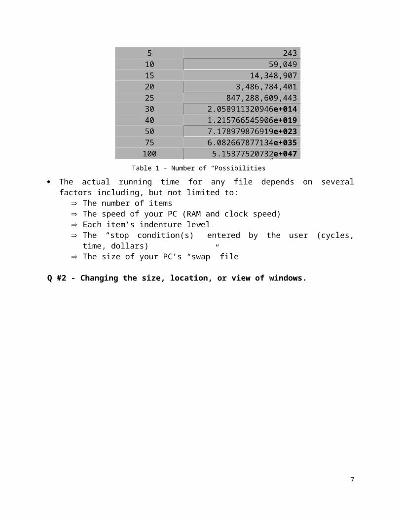
Figure 5 - Scroll button location without "full" window (left); button location with "full" screen (right)

Q #5 - Why can’t I type data into my input fields?

The data input windows listed below require the user to “append” a record before data can be entered. Select “Record” from the Main Menu bar; then select “Append” from the menu...OR...Hit “Ctrl-Enter”:

Y1 - System List E1 - System on End Item S1 - Site List I1 - Item List T2 - Resource List

These data input windows do not require the user to “append” records: G1 - Analysis Parameters G2 - Services G3 - Site Types S2 - Site Setup L1 - Item Characteristics R1 - Repair Site Data T1 - Task Identification T3 - SE at Site

The other most common reason that data cannot be typed into an input field is the field is a “List”. These fields require the data be entered using the “List” command. Whenever “List” appears in the Main Menu bar, you must use it to enter data into that data field (see Figure 6, notice the only difference between the top and bottom screens is the location of the cursor). The following data fields require data entry using the “List” command (the designation code of the input data window is listed in parenthesis after the field name):

System ID (E1) End Item (S2) Next Higher Assembly (I1) Distant Repair Site (R1)

7

Joint Repair Site (R1) Rescue (T1) Support Equipment (T3)

Figure 6 - Normal Main Menu bar (top); Menu bar with "List" (bottom)

Q #6 - The “Automatic Data Paths” in the model do not appear to be operating properly.

There are several instances when the model is suppose to send data automatically from one data field to another or calculate and display a value using several data entries; however, the data is not shown on the screen (see Figure 7 Note that in the top window, the “A-6 Intruders” at “NAS Non-Conus” the model has not made the connection between the “A-6” and “System 2” nor has it calculated the “System Utilization” even though it has all the required data). This happens because the model has not “refreshed” its screen. There are two ways to correct this problem:

1. “Scroll” the record to where the data is suppose to be displayed off the screen and when you scroll back the data will appear...OR

2. “Close” the window where the data should be displayed; when that window is reopened the data will appear.

8

Figure 7 - "Site Utilization" not calculated (top); Same window after "Close" and reopening" (bottom)

9

Q #7 - What is the best screen setup for my input windows?

We recommend “moving” your “System List” to the upper right-hand corner of your screen by placing the cursor in the window “title bar,” click and hold, and drag the window to the position you desire. This allows you to switch between “systems” when required, without having to reopen the System List window.

Size the rest of your input windows so they fit most economically on your screen without blocking “System List,” but displaying as many data fields as possible. The following are examples of how we set up our screen when using JAM for LORA:

Figure 8 - Screen configuration for "System Parameters"

10

Figure 9 - Screen configuration for "System on End Item"

Figure 10 - Screen configuration for "Site Data"

11

Figure 11 - Screen configuration for "Item List"

Figure 12 - Screen configuration for "Item Characteristics"

12

Figure 13 - Screen configuration for "Distant Repair Site" data

Figure 14 - Screen configuration for "Task Data"

13

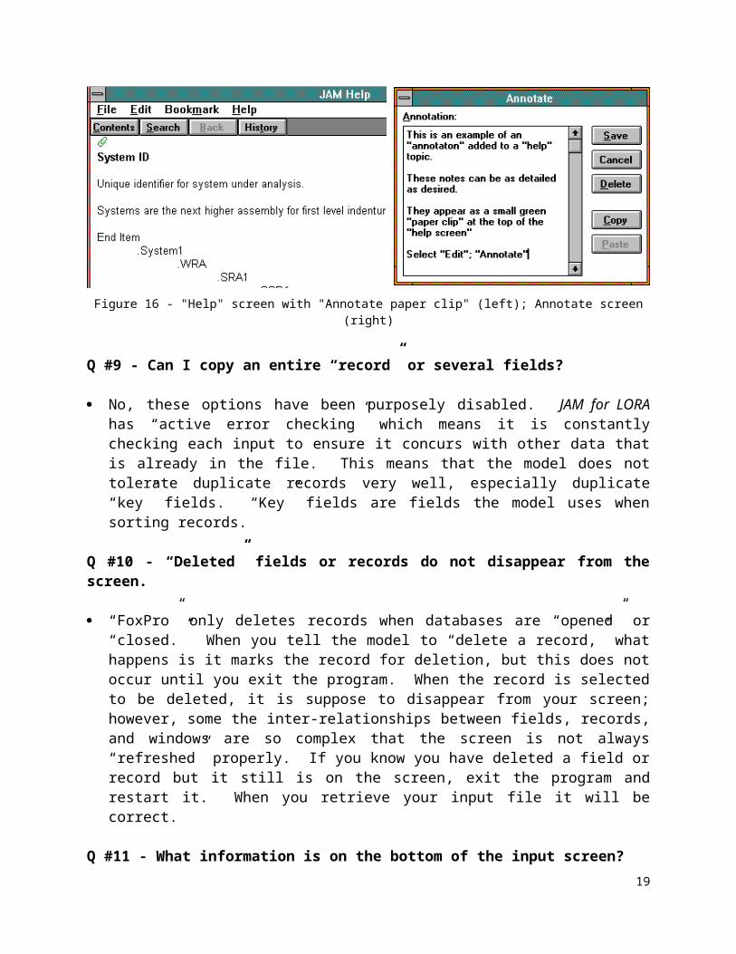
Q #8 - Where are the definitions for the data elements? Is there a “user’s guide’?

A definition for each data element is available via the “Help” feature on the “Main Menu” Bar or by hitting “F1” when the cursor is in the field to be defined.

Figure 15 - Use "Help,” "Search for help on..." or hit "F1"

This software is designed to operate without a user’s guide. Most technical questions concerning data elements or operation of the model should be in the on-line help. If it cannot be found contact us.

Users may add more detail or personal notes to each “help” topic using the “bookmark” and “annotate” features. “Bookmarks” help you quickly locate frequently used help screens. “Annotate” lets the user add detail to data elements definitions that apply to the project they are working on.

14

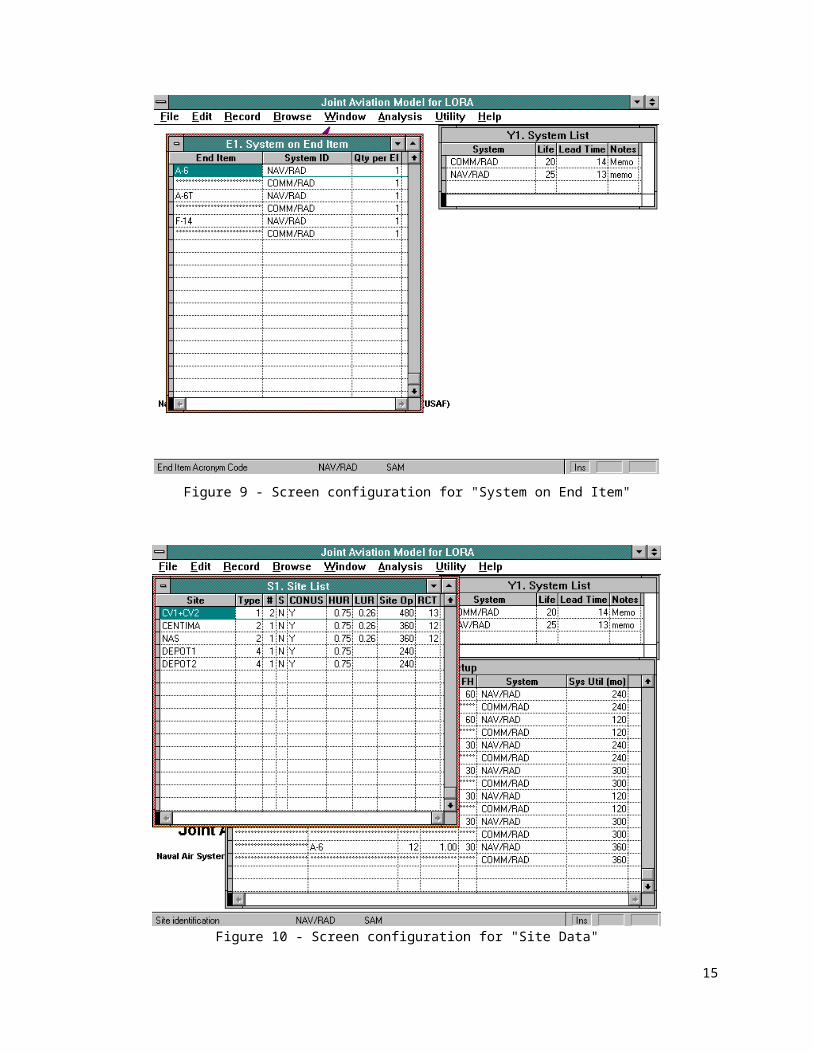
Figure 16 - "Help" screen with "Annotate paper clip" (left); Annotate screen (right)

Q #9 - Can I copy an entire “record” or several fields?

No, these options have been purposely disabled. JAM for LORA has “active error checking” which means it is constantly checking each input to ensure it concurs with other data that is already in the file. This means that the model does not tolerate duplicate records very well, especially duplicate “key” fields. “Key” fields are fields the model uses when sorting records.

Q #10 - “Deleted” fields or records do not disappear from the screen.

“FoxPro” only deletes records when databases are “opened” or “closed.” When you tell the model to “delete a record,” what happens is it marks the record for deletion, but this does not occur until you exit the program. When the record is selected to be deleted, it is suppose to disappear from your screen; however, some the inter-relationships between fields, records, and windows are so complex that the screen is not always “refreshed” properly. If you know you have deleted a field or record but it still is on the screen, exit the program and restart it. When you retrieve your input file it will be correct.

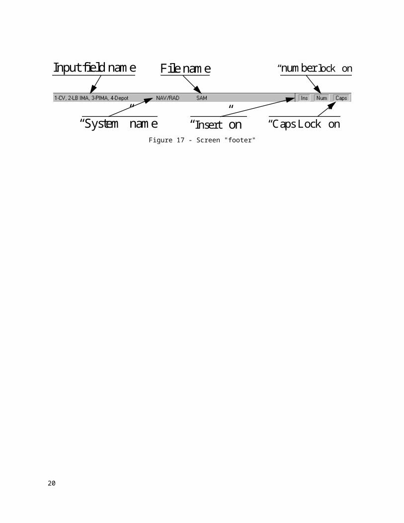
Q #11 - What information is on the bottom of the input screen?

Input field name

“System” name

File name

“Insert” on

“number lock” on

“Caps Lock” onFigure 17 - Screen "footer"

15

Q #12 - How to select more than one item from “LIST”?

There are two ways to select more than one element from a “List” command menu: To select several elements in a row:

place the cursor on the first element to be selected; hit the left mouse button; place the cursor on the last element to be selected; hold down the “shift” key; hit the left mouse button.

Figure 18 - Selecting several "resources" from "List" using the "Shift" key (left); selecting scattered elements using the "Ctrl" key (right)

To select several scattered elements: hold the “Ctrl” key down until all selections are made; place the cursor on the first item to be selected; hit the left mouse button; place the cursor on the next element to be selected; hit the left mouse button; continue in this fashion until all the desired elements have been selected; release the “Ctrl” key.

Q #13- Divide by zero or overflow error when using JAM in an NT environment.

Usually the problem is the security setup on your PC. NT has a switch that does not allow users to copy *.EXE files to the hard disk. This switch must be turned off. On some NT machines an error is displayed when the model is first stated, but if you hit “OK” the model will run properly.

16

Part IIPart II

Using JAM for LORA for Trade-off Studies and Sensitivity Analyses

The Joint Aviation Model for Level Of Repair Analysis is designed to determine the best and most economical maintenance level for corrective maintenance items. The main purpose of the JAM for LORA is to provide a “rational basis” for making the repair level decisions that go into a maintenance plan. It is usually performed early in Engineering Manufacturing Development (EMD) and provides recommendations to APML’s or program offices on how to fashion a maintenance plan for a system. LORA does not determine the maintenance plan.

The model calculates the cost of several “standard” maintenance alternatives, including “discard of all items,” “repair all items at depot,” and “repair all items at IMA.” Additionally, the model estimates the “optimal” maintenance alternative for each input file. The “LORA Life Cycle Cost” of these alternatives and the model’s “Sensitivity Analysis” can be used to perform “regression” analyses to predict when changes in the optimal maintenance alternative will occur. Among the other benefits of collecting all of the data used by JAM is it may be used for studies to determine:

- the minimum required “MTBF” to make an item economically “depot” repair;- the number of pieces of “support equipment” required for each repair site;- if the workload at the depot supports the purchase of new “support equipment” or if the existing equipment can handle additional workload;- the cost difference, over the life cycle of the equipment, if the “MTBF” or some other important parameter changes significantly;- if and how the maintenance plan should change if there are any significant changes to important input parameters;- the difference in LORA life cycle cost of using an alternative other than the “optimal” LORA alternative;- the cost of a “user determined maintenance alternative.”

JAM for LORA uses logistics parameters to estimate the differences in life cycle cost between various maintenance alternatives. The user enters data that describes:

the “sites” where the “items” will be repaired; the interrelationship of the “repair sites”; the “items” being studied; the “item hierarchy”; the characteristics of the “items”; and the “support equipment,” “documentation,” “facilities,” and “training” required

to perform the assigned maintenance tasks.

17

The model uses this data to determine the number of failures for each item at each site, the quantity and cost of support equipment required at each site, and the number of spares required at each site over the life cycle for each maintenance alternatives by calculating:

the number of “failures,” “removals,” “scraps,” and “discards” that occur at each site; the of number of pieces of “support equipment” required for each site; the cost for “inventory,” “labor,” “material,” “transportation,” “AVDLR,” and

“facility space” at each site; and the number of replacement spares required for each site (the number of spares at

each site can be adjusted by setting the “Spares Confidence Level,” a feature unique to this model).

The model uses these calculations to show the differences in cost over the life cycle among different maintenance alternatives. All costs are categorized as either “item costs,” “site costs,” or “system costs.” “Item costs” are costs that are directly attributable to the items under analysis including “inventory,” “labor,” “material,” “transportation,” “scrap rate” and “salvage value”. “Site costs” are those costs that may be influenced by the items but are more directly related to the sites where the items are repaired like “support equipment costs,” “training costs,” and “documentation costs”. “System costs” are those costs incurred regardless of the number of items or sites including “support equipment development costs” and “documentation developments costs.”

All of the model results are printed in output reports or displayed on the screen for the user (see the examples on the following pages). The “Item Disposition Reports” show the number of repairs, discards, scraps, BCM’s, etc... for each site. The report shows how many times each of these actions occur. The “Life Cycle Cost Reports” show the cost by item and site for inventory, labor, transportation, support equipment, etc...These reports show how much each alternative costs. The “Resource Requirements and Support Equipment Utilization” report shows support equipment “loading” calculation results. The “Inventory” reports show costs and number of items required either by site or collectively for each maintenance alternative.

The model also produces graphs directly on the screen. These graphs show the LORA life cycle cost for each alternative broken out by cost category. The user may choose to display either a graph of the “top ten” alternatives as “stacked bars,” a single alternative as a bar chart (not stacked), or the user may edit the graphic using “MSgraph” as desired. The model operates in “Windows” environment the graphs can be copied and printed in other “Windows” compatible word processors or graphic packages.

In addition to the standard uses of the model discussed above the model has many optional uses. The most important alternative uses of the JAM for LORA are:

(1) Sensitivity Analysis - This process tests the susceptibility of the “least cost maintenance alternative” or another specified maintenance alternative to change when an input parameter is varied over a given range. The user selects one of the two types of analyses:

18

(a) “Non-Reoptimize” - which holds the current “maintenance alternative” stable and studies the change in cost of the alternative as the sensitivity parameter is varied; or(b) “Reoptimize” - which allows the model to change the “alternative” as well as cost while the “sensitivity parameter” changes.

(2) Trade-off Analysis - This analysis studies the impact of changing the value of an input parameter on a known maintenance alternative. “Trade-off’s” can be used to study the best distribution of “operating systems,” the “number of sites,” use a “PIMA” or a “depot” as the “final repair site,” use of a “commercial” or “organic” depot, the kind and cost of “support equipment” to be used, etc. “Trade-off analysis” differs from “sensitivity analysis” in that it is done when the user knows the value of the input parameter they wish to study. For instance “what is the impact of 20 IMA sites instead of 30 IMA sites.” “Sensitivity analyses” are performed when the user wants to study the impact of a parameter varying over a wide range.

(3) Breakpoint Analysis - This analysis is used to determine the value of an input parameter at which the “most economical” maintenance alternative switches from one maintenance alternative to another (e.g. it can determine at what “MTBF” does the optimal decision become “repair at depot”) using “regression analysis” techniques.

[The following pages are standard outputs from the JAM for LORA, explanatory notes are in square braces.]

19

EXAMPLESSystemid Item FM LOR

COMM/RAD -> Radar/Rec I -> Rec/Trans I --> Trans/Mod I ---> Blnk/Gen/Ckt/crd I ---> Mod/Ckt/Card I NAV/RAD -> Radio/Rec I --> Corr/Ckt/Crd/Assy I --> IF Proc I --> Pwr/Supp/Subassy 1 X -> Rec/Trans I --> Pwr/Supp/Subassy I ---> Pwr/Supp/Cktassy I ---> Pwr/Supp/Cktassy 1 I -> Rec/Trans 1 X

[These are the items studied in this “sample” model run, their indenture level, and the least cost maintenance alternative for each item as determined by the optimization.]

1 2 3 4 5 6 7 8 9 10-2000

0

2000

4000

6000

8000

10000

12000

14000

16000

18000

1 2 3 4 5 6 7 8 9 10

Optimization ResultsDOC_DEVSE_DEVDOCTRAININGREP_SPACESE_SPACESE_SUPPSESALVAGEAVDLRREP_SCRAPTRANSMATLLABORINV_STORAGINV_ADMININV

[This chart is a “stacked bar” graph. It shows the results of the optimization run using the JAM for LORA for a “sample” data set. Each color represents a different cost category (see legend on the right of the graph). This chart helps determine the most important costs. All of the subsequent data, graphs, and output reports where produced from this data.]

20

Report : Optimization Top Ten Plan : Optimized Run ID : Sam1

PLAN $$ MAINT ALT. 1 14955.0 IIIIIIIIXIIIIX 2 16590.7 IIIDIIIIXIIIIX 3 16592.1 IIIDIIIIXIIIXX 4 16650.7 IIIIDIIIXIIIIX 5 16652.0 IIIIDIIIXIIIXX 6 16656.6 IIIDDIIIXIIIIX 7 16657.9 IIIDDIIIXIIIXX 8 16742.0 IIIDIIIIXIIIII 9 16743.4 IIIDIIIIXIIIXI10 16803.4 IIIIDIIIXIIIXI

[Each bar above corresponds to a “plan” or “maintenance alternative” listed in this report. Each alternative is unique. Each alternative has one cost; however, more than one alternative may have the same cost. These ten alternatives are the “ten best” calculated by the model so far.]

1. Sensitivity analysis run without re-optimization

[The following chart displays the results of a “sensitivity analysis” run by the model using “MTBF”. The MTBF’s in the input file are varied from their original values to 10 times the original values in ten “increments”. All other input parameters remain the same for each increment. Each bar represents one increment of the “sensitivity analysis” run. Each color on the bar indicates the relative contribution of each cost category for that increment. The maintenance alternative is held stable for all increments. This type of sensitivity analysis shows the impact on an existing maintenance plan if an input parameter changes, but the items are repaired at their original maintenance levels. ]

21

1 2 3 4 5 6 7 8 9-2000

0

2000

4000

6000

8000

10000

12000

14000

16000

1 2 3 4 5 6 7 8 9

Sensitivity Results (MTBF)DOC_DEVSE_DEVDOCTRAININGREP_SPACESE_SPACESE_SUPPSESALVAGEAVDLRREP_SCRAPTRANSMATLLABORINV_STORAGINV_ADMININV

[The “Sensitivity Results” list (below) shows the “increment number,” the “LORA life cycle cost” for that increment, and the “sensitivity analysis value”.]

Report : Sensitivity ResultsAnalyzing : Life Cycle Cost of 14955.0 varying MTBF from 1.00 to 50.0

Inc# $$$$$ SA value 1 5273.1 50.00 2 5276.6 44.56 3 5280.6 39.11 4 5305.5 33.67 5 5492.8 28.22 6 5630.5 22.78 7 6007.7 17.33 8 6069.8 11.89 9 6955.5 6.4410 14955.0 1.00

22

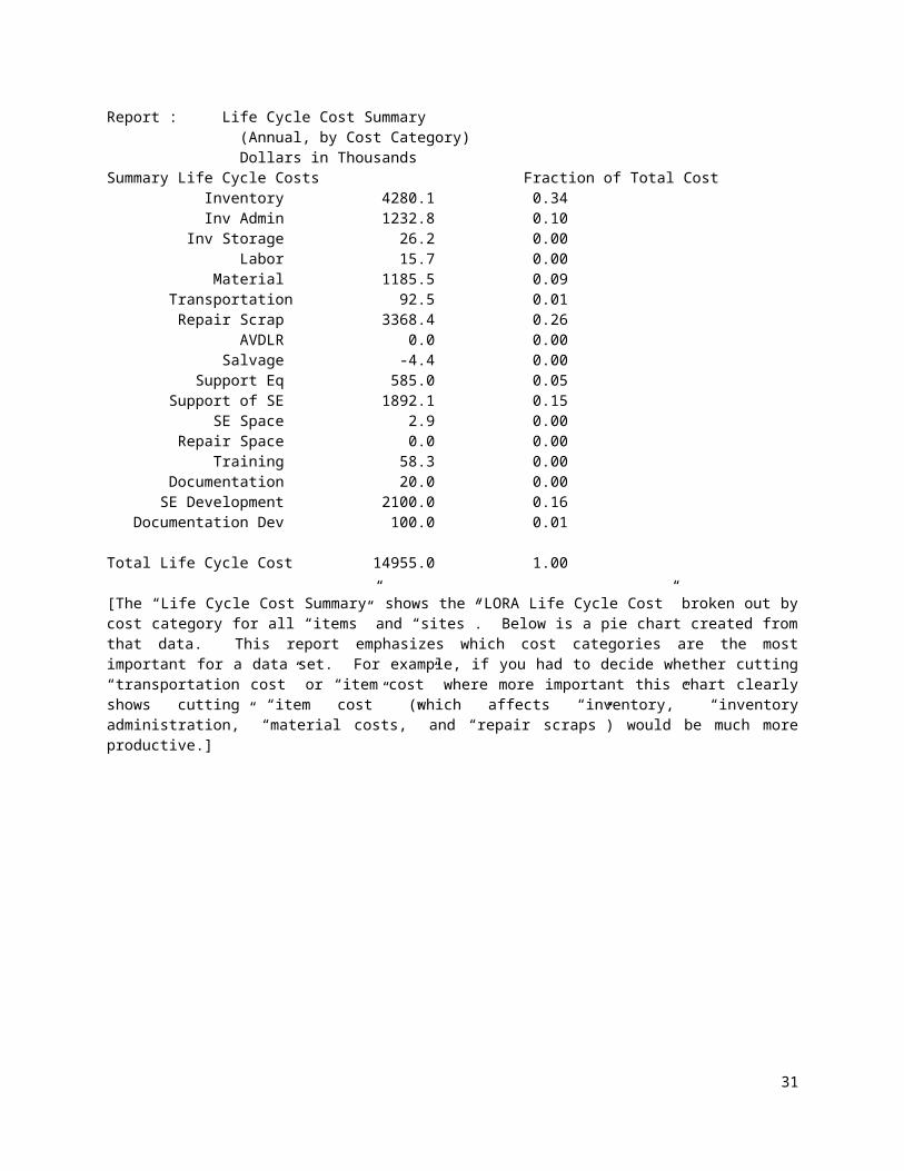
Report : Life Cycle Cost Summary (Annual, by Cost Category) Dollars in ThousandsSummary Life Cycle Costs Fraction of Total Cost Inventory 4280.1 0.34 Inv Admin 1232.8 0.10 Inv Storage 26.2 0.00 Labor 15.7 0.00 Material 1185.5 0.09 Transportation 92.5 0.01 Repair Scrap 3368.4 0.26 AVDLR 0.0 0.00 Salvage -4.4 0.00 Support Eq 585.0 0.05 Support of SE 1892.1 0.15 SE Space 2.9 0.00 Repair Space 0.0 0.00 Training 58.3 0.00 Documentation 20.0 0.00 SE Development 2100.0 0.16 Documentation Dev 100.0 0.01

Total Life Cycle Cost 14955.0 1.00

[The “Life Cycle Cost Summary” shows the “LORA Life Cycle Cost” broken out by cost category for all “items” and “sites”. Below is a pie chart created from that data. This report emphasizes which cost categories are the most important for a data set. For example, if you had to decide whether cutting “transportation cost” or “item cost” where more important this chart clearly shows cutting “item cost” (which affects “inventory,” “inventory administration,” “material costs,” and “repair scraps”) would be much more productive.]

Life Cycle Cost Breakdown (Bar 1)

INV28%

INV_ADMIN8%

INV_STORAG 0%LABOR 0%

MATL8%

TRANS1%

REP_SCRAP23%

AVDLR 0%SALVAGE 0%

SE4%

SE_SUPP13%

SE_SPACE 0%

REP_SPACE 0%TRAINING 0%

DOC 0%SE_DEV

14%DOC_DEV

1%

INVINV_ADMININV_STORAGLABORMATLTRANSREP_SCRAPAVDLRSALVAGESESE_SUPPSE_SPACEREP_SPACETRAININGDOCSE_DEVDOC_DEV

23

Report : Resource Requirements and Support Equipment Utilization (Annual, by Resource/Site) Dollars in Thousands Plan : Optimized Run ID : Sam1Site:DEPOT2 Oper Hrs : 240 SE High Use Rate : 0.75 SE Low Use Rate : 0.00

Resource Type Available Required Utilized Qty Total Remaining ID Hrs Hrs Procured Cost Hrs on SE ---------- ---- --------- --------- ---------- ---------- ---------- ---------- 1SRATPS S 216.0 0.8 0.000 0 0.0 215.2 1WRATPS S 0.0 1.0 0.001 1 40.0 2159.0 2SRATPS S 0.0 3.6 0.002 1 35.0 2156.4 2WRATPS S 432.0 4.0 0.002 0 0.0 428.0 75.0

Report : Inventory Summary (Life Cycle Requirements by Item) Dollars in Thousands Plan : Optimized Run ID : Sam1

Life Life Cycle Unit Init Annual Cycle Level 1/Level 2/Level 3 ( $ ) Cost Stock Acq. Procured

System: COMM/RAD -> Radar/Rec a 50.6 4.6 3.3 2.3 11.0 -> Rec/Trans a 31.5 10.5 0.6 1.0 3.0 --> Trans/Mod 10.3 5.2 0.2 0.6 2.0 ---> Blnk/Gen/Ckt/crd 9.7 4.9 0.0 0.0 2.0 ---> Mod/Ckt/Card 5.0 2.5 0.2 0.6 2.0 System: NAV/RAD -> Radio/Rec a 1710.0 30.0 4.4 1.7 57.0 --> Corr/Ckt/Crd/Assy 95.0 5.0 1.8 1.3 19.0 --> IF Proc 620.0 10.0 5.8 2.2 62.0 --> Pwr/Supp/Subassy 1 0.0 50.0 0.0 0.0 0.0 -> Rec/Trans a 1300.0 100.0 0.9 0.9 13.0 --> Pwr/Supp/Subassy 400.0 50.0 0.6 0.9 8.0 ---> Pwr/Supp/Cktassy 48.0 16.0 0.7 1.1 3.0 ---> Pwr/Supp/Cktassy 1 0.0 16.0 0.0 0.0 0.0 -> Rec/Trans 1 0.0 100.0 0.0 0.0 0.0 --------- -------- --------- --------- --------- Total=> 4280.3 4280.1 18.6 12.8 182.0'a' beside item indicates user selected maintenance alternative.Date: 04/15/96 15:28:38 Dataset: C:\JAM\DATA\SAM

[These pages contain output reports generated by the data in the “sample” input file. The model calculates this data for every maintenance alternative it considers. The “Optimization Top Ten” (above) lists the ten best maintenance alternatives considered by the optimization routine. Each alternative is unique and has one cost. Duplicate maintenance alternatives are “screened out.” “Resource Requirements and Support Equipment Utilization” shows the support equipment “loading” for each site. It shows how many more hours are available on the equipment before another is required at a site. The “Inventory Summary” shows how many items are required for all sites and their cost.]

2. Sensitivity Analysis with Re-Optimization

1 2 3 4 5 6 7 8 9-2000

0

2000

4000

6000

8000

10000

12000

14000

16000

18000

1 2 3 4 5 6 7 8 9

Sensitivity Results (MTBF)DOC_DEVSE_DEVDOCTRAININGREP_SPACESE_SPACESE_SUPPSESALVAGEAVDLRREP_SCRAPTRANSMATLLABORINV_STORAGINV_ADMININV

Report : Level of Repair Decisions Plan : Optimized Run ID : Sam1

Systemid Item FM LOR

COMM/RAD -> Radar/Rec I -> Rec/Trans I --> Trans/Mod I ---> Blnk/Gen/Ckt/crd I ---> Mod/Ckt/Card I NAV/RAD -> Radio/Rec I --> Corr/Ckt/Crd/Assy I --> IF Proc I --> Pwr/Supp/Subassy 1 X -> Rec/Trans I --> Pwr/Supp/Subassy I ---> Pwr/Supp/Cktassy I ---> Pwr/Supp/Cktassy 1 I -> Rec/Trans 1 X

[This is the “optimal” maintenance alternative calculated by the model.]

25

[A Sensitivity Analysis with Re-optimization” is very similar to the previous analysis except the model looks at each alternative in the “Optimization Top Ten” for each increment of the analysis and determines if any are cheaper than the original maintenance alternative. If one of the other alternatives on the “Optimization Top Ten” are cheaper than the original maintenance plan at any increment, the model will indicate it, as seen below.]

Report : Optimization Top Ten Plan : Optimized Run ID : Sam1

PLAN $$ MAINT ALT.

1 14955.0 IIIIIIIIXIIIIX 2 16590.7 IIIDIIIIXIIIIX 3 16592.1 IIIDIIIIXIIIXX 4 16650.7 IIIIDIIIXIIIIX 5 16652.0 IIIIDIIIXIIIXX 6 16656.6 IIIDDIIIXIIIIX 7 16657.9 IIIDDIIIXIIIXX 8 16742.0 IIIDIIIIXIIIII 9 16743.4 IIIDIIIIXIIIXI10 16803.4 IIIIDIIIXIIIXI

Report : Sensitivity Results

Plan : Optimized Run ID : Sam1

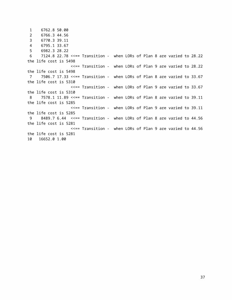
Analyzing : Life Cycle Cost of 16652.0 varying MTBF from 1.00 to 50.0

1 6762.8 50.00 2 6766.3 44.56 3 6770.3 39.11 4 6795.1 33.67 5 6982.3 28.22 6 7124.8 22.78 <<== Transition - when LORs of Plan 8 are varied to 28.22 the life cost is 5498 <<== Transition - when LORs of Plan 9 are varied to 28.22 the life cost is 5498 7 7506.7 17.33 <<== Transition - when LORs of Plan 8 are varied to 33.67 the life cost is 5310 <<== Transition - when LORs of Plan 9 are varied to 33.67 the life cost is 5310 8 7578.1 11.89 <<== Transition - when LORs of Plan 8 are varied to 39.11 the life cost is 5285 <<== Transition - when LORs of Plan 9 are varied to 39.11 the life cost is 5285 9 8489.7 6.44 <<== Transition - when LORs of Plan 8 are varied to 44.56 the life cost is 5281 <<== Transition - when LORs of Plan 9 are varied to 44.56 the life cost is 528110 16652.0 1.00

26

Increment # 1 2 3 4 5 6 7 8 9 10Value (1.00) (6.44) (11.89) (17.33) (22.78) (28.22) (33.67) (39.11) (44.56) (50.00)

Plan # LOR Assignments1 IIIIIIIIXIIIIX 14955.0 ***** ***** ***** ***** ***** ***** ***** ***** *****

2 IIIDIIIIXIIIIX 16590.7 ***** ***** ***** ***** ***** ***** ***** ***** *****

3 IIIDIIIIXIIIXX 16592.1 ***** ***** ***** ***** ***** ***** ***** ***** *****

4 IIIIDIIIXIIIIX 16650.7 ***** ***** ***** ***** ***** ***** ***** ***** *****

5 IIIIDIIIXIIIXX 16652.0 8489.7 7578.1 7506.7 7124.8 6982.3 6795.1 6770.3 6766.3 6762.8

6 IIIDDIIIXIIIIX 16656.6 ***** ***** ***** ***** ***** ***** ***** ***** *****

7 IIIDDIIIXIIIXX 16657.9 ***** ***** ***** ***** ***** ***** ***** ***** *****

8 IIIDIIIIXIIIII 16742.0 ***** ***** ***** ***** 5498 5310 5285 5281 *****

9 IIIDIIIIXIIIXI 16743.4 ***** ***** ***** ***** 5498 5310 5285 5281 *****

10 IIIIDIIIXIIIXI 16803.4 ***** ***** ***** ***** ***** ***** ***** ***** *****

[This chart is an easier way of displaying the results of the “Sensitivity Analysis with Re-optimization”. The first column is the “Optimization Top Ten” alternative number, next is each item’s disposition for each alternative, followed by the LORA Life Cycle Cost for each alternative and increment. “*****” indicates the “LORA life cycle cost” is higher than the “selected” maintenance alternative for that increment (in this case the sensitivity analysis was run for “Plan #5”). The cost for the selected maintenance alternative is shown for all increments. The cost for other increments is shown only if the cost is lower than the “selected” maintenance alternative for a particular increment.]

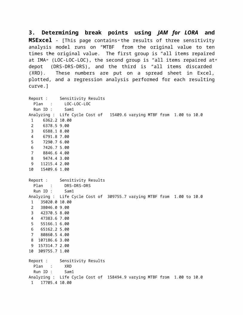
3. Determining break points using JAM for LORA and MSExcel - [This page contains the results of three sensitivity analysis model runs on “MTBF” from the original value to ten times the original value. The first group is “all items repaired at IMA” (LOC-LOC-LOC), the second group is “all items repaired at depot” (DRS-DRS-DRS), and the third is “all items discarded” (XRD). These numbers are put on a spread sheet in Excel, plotted, and a regression analysis performed for each resulting curve.]

Report : Sensitivity Results Plan : LOC-LOC-LOC Run ID : Sam1 Analyzing : Life Cycle Cost of 15409.6 varying MTBF from 1.00 to 10.0 1 6362.2 10.00 2 6378.5 9.00 3 6588.1 8.00 4 6791.8 7.00 5 7290.7 6.00 6 7426.7 5.00 7 8846.6 4.00 8 9474.4 3.00 9 11215.4 2.0010 15409.6 1.00

Report : Sensitivity Results Plan : DRS-DRS-DRS Run ID : Sam1 Analyzing : Life Cycle Cost of 309755.7 varying MTBF from 1.00 to 10.0 1 35020.0 10.00 2 38046.0 9.00 3 42370.5 8.00 4 47383.6 7.00 5 55166.1 6.00 6 65162.2 5.00 7 80860.5 4.00 8 107186.6 3.00 9 157314.7 2.0010 309755.7 1.00

Report : Sensitivity Results Plan : XRD Run ID : Sam1 Analyzing : Life Cycle Cost of 158494.9 varying MTBF from 1.00 to 10.0 1 17705.4 10.00 2 19309.8 9.00 3 21406.8 8.00 4 24052.6 7.00 5 28093.0 6.00 6 32936.0 5.00 7 41308.0 4.00 8 54407.0 3.00 9 80255.5 2.0010 158494.9 1.00

LORA LCC vs MTBF

y = 305253x-0.9509

R2 = 0.9997

y = 156184x-0.9556

R2 = 0.9997y = 14900x-0.393

R2 = 0.9868

0

50,000

100,000

150,000

200,000

250,000

300,000

350,000

33,388 66,776 100,164 133,552 166,940 200,328 233,716 267,104 300,492 333,880

MTBF

LORA

LCC

IMA RepDep Rep

DiscardPower (Dep Rep)

Power (Discard)Power (IMA Rep)

[This chart shows the “data points” from JAM for LORA and the Excel calculated regression curves. “R2” indicates the “quality” of

the fit between the “data points” and the calculated “regression curve”. “1.0” is perfect. You should choose the regression type that provides the “best fit”. The formula shown is the formula for the curve that is drawn.]

30

[To determine at what value of “MTBF” the “least cost alternative” would switch from “repair at IMA” to “repair at Depot” (i.e. the lowest curve on the chart), otherwise known as the “Crossover” point; use the formulas of the lines displayed by Excel. The formula for “Repair at IMA” is set equal to the formula for “Repair at Depot” and solved for the value of “x,” which in this case represents MTBF. In other words we looking for the value of “x” where “y” is equal for both formulas. For this chart the “IMA Repair” line and the “Discard” line cross when x=64 hours; however, these lines are very close to each other, so close that if you assume a 20% margin around the “Repair at IMA” line, as long as the “MTBF” is greater than 161 hours any of these maintenance alternatives is acceptable. A similar set of analyses can be run for “Life cycle,” “Number of Aircraft,” “Operating Hours,” “Number of sites,” etc.. almost any model entry.]

[The following pages contain the “item identification,” “item cost” and “failure” data used to produce the results displayed above. This report shows the “Item Hierarchy” and cost. “Unit Price” is the cost of purchasing a new item. “Net Price” is the “average depot repair cost”. The symbol “->“ indicates the item is a “WRA,” “-->“ means the items is a “SRA,” and “--->“ denotes a “SSRA.”]

Item Identification ==================== System/Item FM Unit Net Qty/ Part # Nomenclature Price Price Sys -------------------- -- -------- -------- ---- --------------- --------------- COMM/RAD -> Radar/Rec 4600 3220 1 xx1 Radar Receiver -> Rec/Trans 10500 7500 1 xx2 Receiver Transmitter --> Trans/Mod 5150 3500 1 xx3 Transmitter Modulator ---> 4850 3300 1 xx4 Blanking Generator Blnk/Gen/Ckt/crd Circuit Card ---> Mod/Ckt/Card 2500 1800 1 xx5 Modulator Circuit Card NAV/RAD -> Radio/Rec 30000 22500 1 x1 Radio Receiver --> 5000 3750 1 x2 Correlator Circuit Corr/Ckt/Crd/Assy Card Assembly --> IF Proc 10000 7500 1 x3 IF Processor --> 1 50000 37500 1 x4 Power Supply Pwr/Supp/Subassy Subassembly -> Rec/Trans 100000 75000 1 x5 Receiver Transmitter --> 50000 37500 1 x6 Power Supply Pwr/Supp/Subassy Subassembly ---> 16000 12000 1 x7 Power Supply Circuit Pwr/Supp/Cktassy Assembly ---> 1 16000 12000 1 x8 Power Supply Circuit Pwr/Supp/Cktassy Assembly -> Rec/Trans 1 100000 75000 1 x9 Receiver Transmitter __________________________________________________________________________

Item Characteristics ==================== System/Item FM Wt (lbs) Vol PPP MTBF OH/FH False FR (cu in) Rem Detect Rate -------------------- -- ---------- ---------- ---- ---------- ----- ------ ------ COMM/RAD -> Radar/Rec 6.00 5184.00 1 2400 1.10 0.03 0.04 -> Rec/Trans 17.00 8640.00 1 800 1.20 0.02 0.03 --> Trans/Mod 5.00 3456.00 4 2500 1.05 0.01 0.02 ---> 5.00 3456.00 10 8000 1.10 0.03 0.04 Blnk/Gen/Ckt/crd ---> Mod/Ckt/Card 2.00 1728.00 8 2600 1.05 0.02 0.03 NAV/RAD -> Radio/Rec 5.00 3456.00 1 638 1.15 0.02 0.03 --> 1.50 1728.00 1 2550 1.00 0.01 0.01 Corr/Ckt/Crd/Assy --> IF Proc 1.50 1728.00 1 850 1.10 0.01 0.02 --> 1 2.00 1728.00 2 1200 1.17 Pwr/Supp/Subassy -> Rec/Trans 5.00 3456.00 1 850 1.20 0.02 0.03 --> 2.00 1728.00 2 2550 1.17 0.02 0.03 Pwr/Supp/Subassy ---> 10.00 6912.00 3 2600 1.10 0.01 0.02 Pwr/Supp/Cktassy ---> 1 10.00 6912.00 3 5000 1.10 Pwr/Supp/Cktassy -> Rec/Trans 1 5.00 3456.00 1 850 1.20 __________________________________________________________________________

[“Item Characteristics” extends the “Item Hierarchy” window. This data defines the size, weight, and failure characteristics for all items. The data in these input windows is “made-up.” It is intended to show what data looks like when loaded in the model. It does not represent any known or planned operating system. It is for demonstration only.]

32

4. Future planned improvements to the JAM for LORA.

Cost of Ownership LORA Data Elements and Algorithms - Identify and incorporate additional data elements and algorithms required to make the JAM for LORA a more “Cost of Ownership” model, including direct and indirect costs. The goal is to create a tool that program managers can use to perform “trade-off studies.” This tool studies the impact of changes in various logistics parameters to reflect how “real world” dollars will be spent.

Advanced Sensitivity Analysis - The sensitivity analysis now used is two dimensional, it varies just one parameter over a given range and the LORA cost at a time. The advanced sensitivity analysis improvement would allow the model to vary two or more input parameters at one time and determine the changes to both the life cycle cost and the least cost maintenance alternative’s decisions. The output would be shown using a color screen or color printer as the output device. This chart must be produced as early in the acquisition process as possible so it may be used to help guide maintenance, logistics, and design engineers.

Readiness Based Sparing - Using RBS, the model would buy spares more closely resembling how ASO (Aviation Supply Office) actually purchases them, trading off an item’s failure rate vs. its cost and indenture level to determine the optimal mix of spares for a system. The Army uses “Availability Based Sparing” in their LORA model called “COMPASS”. This model allows the user to set a “readiness goal”. When the model runs, it determines if the goal can be reached and determines how many spares would be required to obtain that goal. If the ASO model cannot be adapted, COMPASS would make a good starting point.

Automatic Data Paths - Select data elements for the LORA model that are part of another database and create a data path from that location to the LORA model. Identify sources for as many data elements as possible that are reliable, repeatable, available, and accurate. Then develop procedures for collecting this data and updating the LORA database.

Ramp Up\Down the Number of Operating Systems - The current models assume “steady state” aircraft operations over a system’s life cycle. This is a simplistic representation of how operating systems are deployed and retired from the fleet. The model will get better answers if it knows how the systems would be deployed as they arrive in the fleet and begin to operate (ramp up). The model would also keep track of the number of systems as they are withdrawn from the fleet (ramp down).

Long Term Objective - Develop a model that considers and keeps track of the “capacities” of all Naval Aviation maintenance sites (it should be noted however, that defining “capacity” is very difficult). This model would feed data to the LORA model to help determine the “optimal” operational scenario. This “Site Loading” model would have an up-to-date database of each site’s available “capacities” in “support equipment,” “hanger space,” “storage space,” and “man-loading”. The model would identify sites with “existing capacity” and where new systems would “fit” best, that is, cause the Navy to purchase the least amount of “infrastructure” to accommodate the new systems. Or the model could be given an “operational scenario” of a new system and would calculate the infrastructure impact (availability, new hangers, runways, personnel, support equipment, etc...) Unlike LORA models, the “Site Loading” model could

33

keep track of “common” support equipment and how much new equipment would have to be purchased because of the new systems being added to a site. Once the impact of a “site scenario” was determined, it could be sent to the LORA model so the “optimal” decisions could be determined.

34

How the JAM for LORA may be used to help make Commercial -vs- Organic Depot site selections

This section will explain how the JAM for LORA may be used to help determine if the depot for a system should be an “organic” or a “commercial” site. An “organic” depot is any government owned and operated depot including those operated by the Navy, Air Force, or Army. A “commercial” depot is any privately owned site that has won a contract with the Navy, Air Force, or Army to perform depot level maintenance on the system under analysis. A “commercial” site may be either the Original Equipment Manufacturer (OEM) or some third party.

The user should be aware that the JAM for LORA, like any LORA model, has a limited scope. LORA models compare “corrective maintenance” actions performed and the “peculiar” resources (support equipment, documentation, facilities, direct labor, training, etc...) required to perform them. This comparison is based on the cost; to repair an item at an IMA, to repair that item at depot, and to discard that item at depot. The model does not consider “preventive maintenance” tasks or “common” resources (common support equipment, indirect labor, common repair space, etc...). A LORA candidate must be capable of being repaired or discarded at any of the sites listed in the model run. This means that “depot maintenance tasks” cannot be entered into the model. The JAM for LORA is not a absolute life cycle cost model, it compares the relative costs of the one maintenance alternative to another. The analyst and their customer must be aware of these limitations when conducting a “commercial” versus “organic” depot site selection study or reviewing the results.

The method for choosing one depot site over another is to run the model once for each depot site being considered. Each time with data describing a different depot. For example, the first time the data could be for an “organic” or Navy operated depot, and for the second run the data elements would be changed to reflect the costs of a commercial depot. When considering an organic site versus the OEM versus another commercial depot the model would have to be run at least of 3 times.

The steps for determining which depot is best are: Complete the input file for the first depot site. Run the model’s optimization routine to determine the “optimal maintenance alternative”,

another “user specified maintenance alternative”, or “standard alternative” should be selected as a baseline for the comparison.

“optimal” maintenance alternative - the least cost maintenance alternative for a given input file. If any parameter changes, the optimal solution may change.

“user specified” maintenance alternative - the user assigns a maintenance level to one or more items. All other items maintenance level is determined by the optimization routine.

“standard” maintenance alternative - an alternative where all items are assigned a maintenance level by their item indenture level. For example standard alternative (1) is “discard all WRA’s,” (6) is “all WRA’s, SRA’s, and SSRA’s repaired at depot.” There are six standard maintenance alternatives.

35

Print the model’s output reports so the differences created in the analysis can be studied in detail later.

Select the next depot site to be studied and enter its values and repeat the process described above.

Compare the results of each model run. The run with the lowest life cycle cost for the selected maintenance alternative is the preferred depot site.

The input data fields that describe a depot are listed below. These data elements may vary from one depot site to another and may be used to distinguish one depot from another in the JAM for LORA are:

Depot Labor Rate (System Parameters - G3. Site Types) - The cost per hour for direct labor on a LORA candidate. This cost does not include any overhead or indirect costs associated with “depot labor rates.” This data element is ignored by the model if the “AVDLR” switch (AViation Depot Level Repairables) is set to “Y.”

Distant Repair Site Repair Cycle Time (Repair Site Data - R1. Repair Site) - The average total time in days for a LORA candidate to be sent to a depot from an IMA, be repaired, and be returned “ready-for-issue” to the supply system.

Support Equipment already exists at the Depot (Task Data - T3. SE at Site) - A depot may already have a piece of support equipment that any other prospective depot would have to purchase in order to perform the required maintenance tasks in support of the system under analysis. If this is true, use the “SE at Site” window to identify the site, the support equipment, and how much time is left on it before it is fully “loaded.”

Depot Site Operating Hours per Month (Site List - S1. Site List) - The average number hours per month that a particular site is operating (open for business) and available to perform maintenance. It is possible for one depot site to be available significantly less time than a rival. This can affect number of pieces of support equipment required at a site.

Depot Space Cost (System Parameters - G3. Site Types) - The average cost to use a square foot of floor space. This cost measures the relative cost of using floor space for maintenance on aircraft carriers and land based sites. The JAM for LORA Default Data Guide estimates this cost by adding up the annual average all the operating costs of a hanger or other work space (water, power, snow removal, etc...) and dividing by the total area available for maintenance work. This data element is ignored by the model if the “AVDLR” switch is set to “Y.”

Depot Inventory Storage Space Cost (System Parameters - G3. Site Types) - The average cost for a cubic foot of storage space. This cost measures the relative cost of storing spares and equipment for maintenance on aircraft carriers and land based sites. The JAM for LORA Default Data Guide measures this by dividing the “Space Cost” by the average deck height (floor to ceiling height) of a storage area. This data element is ignored by the model if the “AVDLR” switch is set to “Y.”

Depot Attrition Rate (System Parameters - G3. Site Types) - The average annual fraction of personnel turnover. This number is used to determine how many people must be trained each year at a site.

36

When performing a “commercial versus organic” depot site selection LORA, the only differences that can be shown in the JAM for LORA are the in the magnitude of the data elements discussed above. The number of operating aircraft, number of failures, and all other model inputs that may affect the outcome of the model must remain the same for all the depot sites studied. Be aware that the variations in the value of these data elements may cause a change in the least cost maintenance alternative if you are using the “optimal” LORA decision as the decision baseline. If you are doing this, make sure that the optimization routine is run long enough to determine if the “optimal” maintenance alternative has changed.

Persons performing or reviewing this type of analysis should be aware of attempts to “cook the books,” especially those inputs used to distinguish one depot from another. Be aware of any interest or bias an analyst or reviewer may have for selecting one depot over another. This may influence how model runs are performed. All the values for the inputs that affect the depot selection must be verified. It is very easy for one party or the other to enter data elements with a lower value than a competing depot site; however, it may be much more difficult to actualize those numbers in practice.

The final depot sight selection decision should include considerations and costs that are not part the JAM for LORA. These include: number of additional people needed at each site required to support the system under analysis, additional facility costs, overhead costs, and other indirect costs. Non-LORA maintenance actions may have a significant impact on which depot site is best for a particular system. Consider the consequences of any depot site selection on the results of the system’s Reliability Center Maintenance (RCM) program, the Aircraft Service Period Adjustment (ASPA) inspections, and Standard Depot Level Maintenance (SDLM) program.

EXAMPLE

JAM for LORA data elements Depot #1 (organic) Depot #2 (commercial)Depot Labor Rate $30.00 $50.00

Distant Repair Site Repair Cycle Time 55 days 30 daysSupport Equipment already exists N Y

Depot Site Operating Hours per Month 240 100Depot Space Cost $4.50 $10.00

Depot Inventory Storage Space Cost $.45 $.45Depot Attrition Rate .04 .03

AVDLR N N

37

Figure 19 - Examples of the Input Data Fields that can be changed when performing a Commercial vs. Organic Depot Site Selection

Report : Level of Repair Decisions Plan : Optimized Run ID : Joint Sample Problem

Systemid Item FM LOR

AN/ASH-37 (C-130) -> Data Entry Keyboad D --> Front Panel Assmbl D --> Rear Case Assembly D -> Memory Unit D --> Memory PWB Assemby D -> Motion Pickup Tras D -> Recorder Converter D --> Analog I PWB Assy D --> Analog II PWB Assy D --> CPU PWB Assembly DAN/ASH-37 (F-14A) -> Power Supply PWB A D --> Power Supply CCA D

Note: The items listed above from top to bottom are in the same order in each of the “Item Dispositions” from left to right.

38

Organic Depot Commercial DepotTop TenList

Cost($K)

ItemDispositions

Cost($K)

ItemDispositions

1 8454.0 DDDDDDDDDDDD 8467.9 DDDDDDDDDDDD2 8539.2 DDXDDDDDDDDD 8555.0 DDXDDDDDDDDD3 8578.0 DDDDDDDDXDDD 8580.1 DDDDDDDDDDXX4 8609.4 DDDDDDDXDDDD 8594.8 DDDDDDDDXDDD5 8646.8 DDDDDDDDXDDX 8623.1 DDDDDDDXDDDD6 8663.2 DDXDDDDDXDDD 8681.9 DDXDDDDDXDDD7 8685.9 DDDDDDDDXDXX 8693.4 DDDDDDDXDDDX8 8694.5 DDXDDDDXDDDD 8707.0 DDDDDDDDXDXX9 8717.2 DDDDDDDXDDXX 8710.3 DDXDDDDXDDDD10 8731.9 DDXDDDDDXDDX 8735.3 DDDDDDDXDDXX

Notes concerning this example Organic vs. Commercial Depot JAM for LORA site selection: No proprietary data has been used. A full optimization was performed for each data set. The Top Ten Lists are similar but not the same. Each letter position in each Item Disposition corresponds to the same item. The Level Of Repair Dissociation report on the previous page indicates which item

each letter position corresponds to.

Conclusions:

The JAM for LORA may be use to perform Organic versus Commercial Depot Site Selections.

The analysis is limited in scope. The final depot site selection decision should be based on more than just the results of the

JAM for LORA comparison.As you can see from the example model runs, the cost difference between depots may not be large.

39

Part IIIPart IIIInterpreting JAM for LORA stacked bar charts

1 2 3 4 5 6 7 8 9 10-1000

0

1000

2000

3000

4000

5000

6000

7000

8000

9000

1 2 3 4 5 6 7 8 9 10

Optimization ResultsDOC_DEVSE_DEVDOCTRAININGREP_SPACESE_SPACESE_SUPPSESALVAGEAVDLRREP_SCRAPTRANSMATLLABORINV_STORAGINV_ADMININV

This graph shows the results of a JAM for LORA Genetic Algorithm optimization. These are the “Top Ten” maintenance alternatives, also called the “Hall of Fame,” calculated by the model during the most recent optimization run.

The Y-axis shows the life cycle cost in thousands of dollars. Each bar shows the relative value of each of the cost categories listed below.

Please note that the costs appear in the bar in the order in which they are shown in the legend, except “Salvage” which appears as a negative value. All costs are calculated for each bar; however, some costs may be too small to appear on a particular bar.

You may change the format of this chart by placing your mouse anywhere on the chart and double clicking. This calls Microsoft Graph 5.0 (if you get an error message you need to edit your WIN.INI file; see details by selecting “Help” from the main menu and searching on “MSGraph 5.0”). Changing the format of the graph will change the graph that appears in JAM for LORA during a Genetic Algorithm run. The original graph can be reset by reloading the model using the “setup” routine

40

DOC_DEV

SE_DEV

DOC

TRAINING

REP_SPACE*

SE_SPACE

SE_SUPP

SE

SALVAGE*

AVDLR*

REP_SCRAP

TRANS*

MATL

LABOR*

INV_STORAG*

INV_ADMIN

INV

* Indicates that these cost categories are not proportionally large enough to appear on this bar

41

Costcategory

Category Name Definition

DOC_DEV document development cost to develop all documents; non-recurring costSE_DEV support equipment development cost to develop support equipment; non-recurring costDOC documentation document unit cost; per site costTRAINING training cost to provide training; number of people to be

trained times the training costREP_SPACE repair working space cost to use floor space; site type space cost times the

number of square feet required

SE_SPACE support equipment space cost to use/store support equipment; site type space cost times the number of square feet required

SE_SUPP support equipment support cost of support of support equipment; SE unit cost times Support of SE fraction times life cycle

SE support equipment support equipment unit cost times the number of sites using the SE times the number of SE required per site

SALVAGE salvage value total scrapped and discarded items times each item’s unit cost times the salvage rate

AVDLR aviation depot level repairables total cost to repair items at the depot less the cost of SE

REP_SCRAP repair scrap cost to replace scrapped items; total failures times scrap rate times the unit cost

TRANS transportation cost to ship items; item weight times distance between sites times shipping rate

MATL material cost of non-LORA items/ equipment/ material; item cost times material rate

LABOR labor cost of direct labor; labor rate times maintenance time times number of maintenance actions

INV_STRORAG inventory storage cost to store spares; volume times number of item spares

INV_ADMIN inventory administration cost administrative support for spares; field supply admin cost times number of items times total number of sites

INV inventory spares cost; item cost times number of spares required

42

Part IVPart IVInternal workings of JAM for LORA

1. - Updating WIN.INI to MSgraph 5.0

If you get this error message when you double click on a graph...

You will get slightly different error messages from Windows 95, but the process should be very similar. (See the end of this message for details.)

Explanation: Windows has a built-in graphics package that programs may use to create charts and graphs called “MSgraph.” Unfortunately, there are two versions of “MSgraph”; “MSgraph” and “MSgraph 5.0.”

“MSgraph 5.0” is, by far, the better of the two programs. “MSgraph 5.0” is compatible with “MSgraph” and does everything it does, plus “MSgraph 5.0” does more. The problem is “MSgraph” will not read “MSgraph 5.0” files. JAM for LORA creates its charts using “MSgraph 5.0” so it can take advantage of the greater capabilities, however some PC’s are not setup to use 5.0.

Follow these steps to setup your PC so you can edit JAM for LORA graphs/charts.

1. If you are still inside JAM for LORA:

a. - Print this page.b. - Save the model run.c. - Exit JAM for LORA to Windows.

2. Start SYSEDIT (from Program Manager).

a. - Select FILE.

43

b. - Select RUN...c. - Enter “Sysedit”; this opens several windows in the Sysedit program.d. - Close all windows except WIN.INI, including AUTOEXEC.BAT, CONFIG.SYS, and SYSTEM.INI. Sysedit is a text editor and we do not want to make any changes to these other files by accident.

3. Change “MSgraph” to “MSgraph 5.0”

a. - Select SEARCH.b. - Select FIND...c. - Enter “msgraph”; hit enter.d. - Hit F3 until the cursor is on a line that looks like the following (usually just once more):

MSGraph=Microsoft Graph,MSGraph,C:\WINDOWS\msapps\msgraph\graph.exe,pictureMSGraph.Chart.5=Microsoft Graph 5.0,Microsoft Graph5.0,C:\WINDOWS\MSAPPS\MSGRAPH5\GRAPH5.EXE,picture

[Note: Both lines end with the word “picture”. These lines may differ in some details because your file path may not be the same as mine.]

e. - Change each file path from “MSgraph” to the path for “MSgraph 5.0” by adding a “5” after “MSGRAPH” and after “GRAPH”. The new lines should look like this:

MSGraph=Microsoft Graph 5.0,MS Graph,C:\WINDOWS\msapps\msgraph5\graph5.exe,pictureMSGraph.Chart.5=Microsoft Graph 5.0,Microsoft Graph 5.0,C:\WINDOWS\MSAPPS\MSGRAPH5\GRAPH5.EXE,picture

4. Save and initialize:

a. - Select FILE.b. - Select SAVE.c. - Select FILE.d. - Select EXIT.e. - Select FILE (you must exit Windows to DOS and reenter to initialize the changes we just made).f. - Select EXIT WINDOWS...g. - Click OK.

You may now re-enter Windows, run the same JAM for LORA file, and now you will be able to edit the graphs produced when the Genetic Algorithm is run.

44

2. - How to change a bar chart to a pie chart in MSGraph 5.0

a. Begin from JAM for LORA with a stacked bar chart showing (default):

b. - Select the maintenance plan that you wish to convert to a pie chart (in the figure above, maintenance alternative #5 is selected).

c. - Select GRAPHICS.

d. - Select DETAIL, then DONE; this changes the displayed chart to the following (see Figure 32 on the next page):

e. - Double click on this chart to enter MSGraph 5.0; notice there are two windows in MSGraph, one with displays the data and the other that shows the chart. To create a pie graph in the chart window we are going to use both the menu and the data window.

45

5-500

0

500

1000

1500

2000

2500

3000

3500

4000

5

Life Cycle Cost Breakdown (Bar 1)INVINV_ADMININV_STORAGLABORMATLTRANSREP_SCRAPAVDLRSALVAGESESE_SUPPSE_SPACEREP_SPACETRAININGDOCSE_DEVDOC_DEV

Figure 20 - JAM for LORA "Detail" graphic for a maintenance alternative

f. - Change from “Series in Columns” (right button - “by column”) to “Series in Rows” (left button - “by rows”).

g. - Select the “Chart type” button. Then select the type of chart you wish to display. For this example, choose the 3-D pie from the menu.

3. - Notes on the Sensitivity Analysis of the LORA model

CONCERN #1 - How do the Default Data Guide (DDG) entries affect the results of the LORA model?

The DDG entries have an impact, but not a decisive impact on the results of the LORA model. These entries set up a framework that the more important model entries operate on.

The value of DDG entries do not tend to change by any significant amount over time.

The regressions performed on this model were extended to the maximum size the field definition the data element would allow. This was done to study the effect of the input over the widest possible range on the output of the model.

46

The DDG inputs can be divided into three categories that show there relative impact on the results of the model. Although none of these data elements are decisive in determining the LORA, some of the elements have a greater impact than others. Each DDG data element was designated to have either a “strong” influence, a “weak” influence, or a “marginal” influence. “Strong” indicates the data element had a relatively larger impact on the model results that the other data elements that were studied. “Weak” means the data element had a relatively smaller impact that the other data elements. Those elements listed as “marginal” had an impact greater than the “weak” elements but less than the “strong” data elements.

Strong data elements [The Default Data Guide provides a method for estimating the cost of these data elements, but does not provide a value for them.]

Documentation Cost Packaging Cost Transportation Cost

Marginal data elements Item Entry & Retention Cost Field Supply Administration Cost Space Cost Inventory Cost Labor Rate Training Cost Local Repair Cycle Time Depot Repair Cycle Time

Weak data elements Required Days of Stock Support Equipment High Use Rate Net Price Surcharge Attrition Rate

CONCERN #2 - Identify the ten most important LORA data elements used by the model other than those considered by the DDG study.

Strong data elements Mean Time Between Failure Mean Time Between Failure Degradation Factor Life cycle Number of Aircraft Number of Aircraft Flight Hours

Marginal data elements Item Cost Support Equipment Cost Material Rate

47

Weak data elements BCM Rate Net Price

Although “Item Cost” and “Support Equipment Cost” are both identified as “marginal” data elements they are extremely important to the model in determining the optimal LORA results. Both of these data elements are strongly effected by the number of IMA sites, number of failures, number of aircraft, and number of flight hours identified in the input file. They are usually identified as the most important LORA data elements along with the MTBF. This is because these three data elements not only have a relatively greater influence on the model results than most inputs, they are also the most volatile inputs the model uses (i.e. likely to change).

4. - Location of data in JAM for LORA files

Table Name Alias(s) Description

file01.JDF System Call up the filefile02.DBF Item [I1, L1] Item/ System/ Next Higher Assembly

file03.DBF EI_Site [S1] End Item at Sitefile04.DBF Odrs [R1] Distant Repair Sitefile05.DBF Jdrs [R1] Joint Distant Repair Site

file06.DBF Res_Site [T3] SE Availability at a Sitefile07.DBF Task [T1] Task Identificationfile08.DBF Task_Res [T1] Task Identification (cont)file09.DBF Sys_EI [E1] System on End Items

file10.DBF End Item [Y1] End Item Listfile11.DBF Site [S1] Site Definitionfile12..DBF Resource [T2] Task Resource Listfile13.DBF Service [G2] Service Specific Datafile14.DBF SiteType [G3] Site Type Attributesfile15.DBF Parm [G1] Analysis parameters and global data

Note: “File” is user entered name when creating a new dataset. Datasets may contain one or more systems. End Items placed at Sites within the dataset contain the systems identified. Files 16.dbf - 19.dbf contain results of the model’s preliminary calculations.

48

List of FiguresFigure 1 - Window control features_________________________________________________________________Figure 2 - Sizing a window_______________________________________________________________________Figure 3 - Character Editing______________________________________________________________________Figure 4 - (left) Window when it is opened; (right) window scrolled up____________________________________Figure 5 - Scroll button location without "full" window (left); button location with "full" screen (right)__________Figure 6 - Normal Main Menu bar (top); Menu bar with "List" (bottom)___________________________________Figure 7 - "Site Utilization" not calculated (top); Same window after "Close" and reopening" (bottom)__________Figure 8 - Screen configuration for "System Parameters"_______________________________________________Figure 9 - Screen configuration for "System on End Item"_______________________________________________Figure 10 - Screen configuration for "Site Data"______________________________________________________Figure 11 - Screen configuration for "Item List"______________________________________________________Figure 12 - Screen configuration for "Item Characteristics"_____________________________________________Figure 13 - Screen configuration for "Distant Repair Site" data__________________________________________Figure 14 - Screen configuration for "Task Data"_____________________________________________________Figure 15 - Use "Help,” "Search for help on..." or hit "F1"_____________________________________________Figure 16 - "Help" screen with "Annotate paper clip" (left); Annotate screen (right)_________________________Figure 17 - Screen "footer"_______________________________________________________________________Figure 18 - Selecting several "resources" from "List" using the "Shift" key (left);____________________________Figure 19 - Examples of the Input Data Fields that can be changed when performing a Commercial vs. Organic

Depot Site Selection_______________________________________________________________________38Figure 20 - JAM for LORA "Detail" graphic for a maintenance alternative_______________________________46

49