uncertainty, sensitivity analysis and the role of data based ... · hydrology and earth system...

Hydrol. Earth Syst. Sci., 11, 1249–1266, 2007www.hydrol-earth-syst-sci.net/11/1249/2007/© Author(s) 2007. This work is licensedunder a Creative Commons License.

Hydrology andEarth System

Sciences

Uncertainty, sensitivity analysis and the role of data basedmechanistic modeling in hydrology

M. Ratto1, P. C. Young2,3, R. Romanowicz2, F. Pappenberger2,4, A. Saltelli1, and A. Pagano1

1Joint Research Centre, European Commission, Ispra, Italy2Centre for Research on Environmental Systems and Statistic, Lancaster University, Lancaster, UK3Centre for Resource and Environmental Studies, Australian National University, Canberra, Australia4European Centre for Medium-Range Weather Forecasts, Reading, UK

Received: 7 April 2006 – Published in Hydrol. Earth Syst. Sci. Discuss.: 25 September 2006Revised: 14 March 2007 – Accepted: 29 March 2007 – Published: 3 May 2007

Abstract. In this paper, we discuss a joint approach to cal-ibration and uncertainty estimation for hydrologic systemsthat combines a top-down, data-based mechanistic (DBM)modelling methodology; and a bottom-up, reductionist mod-elling methodology. The combined approach is applied tothe modelling of the River Hodder catchment in North-WestEngland. The top-down DBM model provides a well identi-fied, statistically sound yet physically meaningful descrip-tion of the rainfall-flow data, revealing important charac-teristics of the catchment-scale response, such as the na-ture of the effective rainfall nonlinearity and the partition-ing of the effective rainfall into different flow pathways.These characteristics are defined inductively from the datawithout prior assumptions about the model structure, otherthan it is within the generic class of nonlinear differential-delay equations. The bottom-up modelling is developed us-ing the TOPMODEL, whose structure is assumed a prioriand is evaluated by global sensitivity analysis (GSA) in or-der to specify the most sensitive and important parameters.The subsequent exercises in calibration and validation, per-formed with Generalized Likelihood Uncertainty Estimation(GLUE), are carried out in the light of the GSA and DBManalyses. This allows for thepre-calibrationof the the priorsused for GLUE, in order to eliminate dynamical features ofthe TOPMODEL that have little effect on the model outputand would be rejected at the structure identification phaseof the DBM modelling analysis. In this way, the elementsof meaningful subjectivity in the GLUE approach, whichallow the modeler to interact in the modelling process byconstraining the model to have a specific form prior to cali-bration, are combined with other more objective, data-basedbenchmarks for the final uncertainty estimation. GSA playsa major role in building a bridge between the hypothetico-deductive (bottom-up) and inductive (top-down) approaches

Correspondence to:M. Ratto([email protected])

and helps to improve the calibration of mechanistic hydro-logical models, making their properties more transparent. Italso helps to highlight possible mis-specification problems,if these are identified. The results of the exercise show thatthe two modelling methodologies have good synergy; com-bining well to produce a complete joint modelling approachthat has the kinds of checks-and-balances required in prac-tical data-based modelling of rainfall-flow systems. Such acombined approach also produces models that are suitablefor different kinds of application. As such, the DBM modelconsidered in the paper is developed specifically as a vehi-cle for flow and flood forecasting (although the generalityof DBM modelling means that a simulation version of themodel could be developed if required); while TOPMODEL,suitably calibrated (and perhaps modified) in the light of theDBM and GSA results, immediately provides a simulationmodel with a variety of potential applications, in areas suchas catchment management and planning.

1 Introduction

Uncertainty estimation is a fundamental topic in hydrologyand hydraulic modelling (see discussion in Pappenberger andBeven (2006) and Pappenberger et al. (2006a)). Mathemat-ical models are always an approximation to reality and theevaluation of the uncertainties is one of the key research pri-orities in every modelling process. The most widely used ap-proach to modelling is based on the description of physicaland natural systems by deterministic mathematical equationsbased on well known scientific laws: the so-called reduc-tionist (bottom-up) approach. Uncertainty estimation is dealtwith via calibration and estimation procedures that insert thedeterministic approach into a stochastic framework (see a re-cent review in Romanowicz and Macdonald (2005) and thereferences cited therein).

Published by Copernicus GmbH on behalf of the European Geosciences Union.

1250 M. Ratto et al.: Uncertainty, sensitivity analysis and the role of data

A widely used approach to calibration in hydrology, andenvironmental sciences in general, is the Generalised Like-lihood Uncertainty Estimation (GLUE, Beven and Binley,1992). This is a very flexible, Bayesian-like approach to cal-ibration, which is based on the acceptance that different pa-rameterisations, as well as different model structures, can beequally likely simulators of the observed systems (referred tovariously as “ambiguity”, “unidentifiability” or “model equi-finality”). In GLUE, model realisations are weighted andranked on a likelihood scale, via conditioning on observa-tions, and the weights are used to formulate a cumulativedistribution of predictions.

In the calibration (model identification and estimation)framework, the understanding, rather than just the evalua-tion of the influence of different uncertainties on the mod-elling outcome, becomes a fundamental question. This is es-pecially the case if the modelling goal is to reduce the modeluncertainties and resources for this task are limited. Globalsensitivity analysis (GSA) can play an important role in thisframework: it can help in better understanding the modelstructure, the main sources of model output uncertainty andthe identification issues (Ratto et al., 2001). For instance,Pappenberger et al. (2006b, c, 2007) and Hall et al. (2005)have recently presented cases that achieve such an under-standing for flood inundation models, using sensitivity anal-ysis to support their analysis. Tang et al. (2006) also providean interesting review of GSA methods within the context ofhydrologic modelling.

The GLUE approach provides a methodology for cop-ing with the problems of lack of identification and over-parameterisation inherent in the reductionist approach, whilea detailed GSA can make these problems more transparent.Neither of the two approaches, however, can provide a fullsolution of these problems.

Another approach to coping with uncertainty in envi-ronmental processes is the “top-down” Data-Based Mech-anistic (DBM) method of modelling, introduced by Youngover many years (see Young, 1998, and the prior referencestherein). Here, the approach is inductive: the models arederived directly from the data based on a generic class ofdynamic models (here, differential-delay equations or theirdiscrete-time equivalents). In particular, the DBM approachis based on the statistical identification and estimation of astochastic dynamic relationship between the input and outputvariables using advanced time series analysis tools, with pos-sible non-linearities introduced by means of non-linear State-Dependent Parameter (SDP) transformation of the modelvariables. Unlike “black-box” modelling, however, DBMmodels are only accepted if the estimated model form can beinterpreted in a physically meaningful manner. This DBMmethodology can also be applied to the analysis and sim-plification of large deterministic models (e.g., Young et al.,1996).

In contrast to the GLUE technique, the DBM approachchooses, from amongst all possible model structures, only

those that are clearly identifiable: i.e., those that have aninverse solution in which the model parameters are welldefined in statistical terms. Moreover, this technique es-timates the uncertainty associated with the model parame-ters and variables, normally based on Gaussian assumptions.If the Gaussian assumptions are strongly violated, however,the DBM analysis exploits Monte Carlo Simulation (MCS)to evaluate the uncertainty. For instance, it is common inDBM analysis to estimate the uncertainty in derived physi-cally meaningful model parameters, such as residence timesand flow partition parameters, using MCS analysis. Also,when the identified model is nonlinear, then the uncertaintyin the state and output variables (e.g. internal, unobservedflow variables and their combination in the output flow) isnormally evaluated using MCS analysis.

In this paper, we will discuss the problems of calibrationand uncertainty estimation for hydrologic systems from aunified point of view, combining the bottom-up, reduction-ist TOPMODEL with the top-down, DBM approach, whichplays the role of an “independent” benchmark. Note that,in this respect, we do not pursue any competitive compari-son, to judge or prove one type of model to be “better” thanthe other. Our choice of DBM modelling as the right can-didate for benchmarking, is based on its capability of pro-viding a meaningful description of observations, in additionto its simplicity, ease of interpretation and rapidity of imple-mentation. We will also highlight the role of GSA in build-ing a bridge between the two approaches by assisting in theimproved calibration of reductionist models and highlight-ing both their weaknesses and strengths. Initially, however,we will compare and contrast the two modelling approachesused in the paper.

2 The Different Modelling Approaches

Data-based Mechanistic (DBM) modelling is a methodolog-ical approachto model synthesis from time-series data and itis not restricted to rainfall-flow modelling; nor, indeed, to thespecific rainfall-flow model identified in the present paper.Its application to rainfall-flow processes goes back a longway (Young, 1974) but the more powerful technical tools forits application have been developed much more recently (seee.g. Young, 1998, 2003 and the prior references therein).

DBM models are obtained by a relatively objective induc-tive analysis of the data, with prior assumptions kept to theminimum but with the aim of producing a model that can beinterpreted in a reasonable, physically meaningful manner.Essentially, DBM modelling involves four stages that exploitadvanced methods of time series analysis: data-based identi-fication of the model structure based on the assumed genericmodel form; estimation of the parameters that characterizethis identified model structure; interpretation of the estimatedmodel in physically meaningful terms; and validation of theestimated model on rainfall-flow data that is different from

Hydrol. Earth Syst. Sci., 11, 1249–1266, 2007 www.hydrol-earth-syst-sci.net/11/1249/2007/

M. Ratto et al.: Uncertainty, sensitivity analysis and the role of data 1251

the calibration data used in the identification and estimationanalysis.

In the case of thespecificDBM model used in the presentpaper, the identification stage of the modeling is based on thenon-parametric estimation of a nonlinear State-DependentParameter (SDP) transfer function model, where the SDP re-lationships that define the nonlinear dynamic behaviour ofthe model are estimated initially in a non-parametric, graph-ical form, with the SDPs plotted against the states on whichthey are identified to be dependent. In the case of rainfallflow models, there is normally only one such SDP relation-ship: this is associated with the rainfall input and the statedependency is identified, paradoxically at first, in terms ofthe measured flow variable (see later). In physical terms,this nonlinear function defines the connection between themeasured rainfall and the “effective rainfall”, i.e. the rainfallthat is effective in causing flow variations. The relationshipbetween this effective rainfall and the flow is then normallyidentified as a linear, constant coefficient, dynamic processand is estimated in the form of a 2nd (or on rare occasions3rd) order Stochastic Transfer Function (STF) model, whoseimpulse response represents the underlying unit hydrographbehaviour. This STF model is the discrete-time equivalent ofa continuous-time differential-delay equation and it could beidentified in this form, if required (e.g. Young, 2005).

In the estimation stage of the DBM modelling, the non-parametric SDP nonlinearity is parameterised in a parsimo-nious (parametrically efficient) manner. Normally, this pa-rameterisation is in terms of a power law or an exponen-tial function, although this depends upon the results of thenon-parametric identification, as discussed in the later ex-ample. The approach used in this paper has been devel-oped in the previously published DBM modeling of rainfallflow processes. Here, the STF model and the power law pa-rameters, are estimated simultaneously using a special, non-linear least squares optimisation procedure that exploits theRefined Instrumental Variable (RIV) transfer function esti-mation algorithm in the CAPTAIN Toolbox for Matlab (seehttp://www.es.lancs.ac.uk/cres/captain/). Depending on theapplication of the DBM model, this simple optimisation pro-cedure can be extended to handle a more sophisticated modelof the additive noise process that includes allowance for bothautocorrelation and heteroscedasticity (changing variance).In the case of the heteroscedasticity, the variance is normallyconsidered as a SDP function of the flow, with higher vari-ance operative at higher flows.

The physical interpretation of this estimated DBM modelis normally straightforward. As pointed out above, the in-put SDP function can be considered as an effective rainfallnonlinearity, in which the SDP is dependent on the flow. Al-though unusual at first sight, this state dependency makesphysical sense because the flow is acting simply as a surro-gate for the soil moisture content in the catchment (catch-ment storage: see the previously cited references). Thus,when the flow is low, implying low soil moisture, the rainfall

is multiplied by a small gain and the effective rainfall is at-tenuated; whilst at high flow and soil moisture, this gain andthe associated effective rainfall are large, so that the rainfallhas a much larger effect on the flow.

The effective rainfall is the input to the STF part of themodel, which characterises the dominant catchment dynam-ics and defines the underlying catchment scale hydrograph.Typically, this 2nd order STF model can be decomposed intoa parallel form that reveals the major identified flow path-ways in the effective rainfall-flow system. These normallyconsist of a “quick” flow component, with a short residencetime (time constant) that seems to account for the surface andnear surface processes; and a “slow” component with a longresidence time, that often can be associated with the replen-ishment of the groundwater storage and the consequent dis-placement of groundwater into the river channel. Of course,it must be emphasised that these components are unobserved(not measured directly) and so their identification is done viastatistical inference based on the specific model form: in thiscase, a generic nonlinear differential equation, the specificstructure of which is identified from the data with the mini-mum of a priori assumptions.

The situation is quite different in the case of TOPMODEL(Beven and Kirkby, 1979), which has the specific modelstructure that is assumed a priori and so constrains the es-timation of the component flows. Consequently, the flowdecompositions of the DBM model and TOPMODEL arequite different. Moreover, in both cases, the interpretationof the decomposed flow components is subjective, depend-ing not only on the model form but also on how the modellerviews the unobserved flow components within the hydrolog-ical context.

Any model of a real system is only acceptable in tech-nical terms if it can be well validated. The final validationstage in DBM modelling is similar to that used for TOP-MODEL and most other hydrological modelling exercises.The model estimated on the calibration data set is applied,without re-estimation, to a new set (or sets) of rainfall-flowdata from the same catchment. If this validation is successful,in the sense that the simulated output of the model matchesthe measured flow to within the uncertainty levels quantifiedduring the model estimation (calibration), then the model isdeemed “conditionally valid” and can be used in whatevercapacity it is intended.

It must be emphasized again that DBM modelling is a sta-tistical approachto model building and any specific DBMmodel will depend upon the objectives of the modelling ex-ercise. For instance, the DBM model for the River Hodder, asconsidered in this paper, is intended primarily for use in dataassimilation and flow forecasting (see Young, 1998, 2003),rather than simulation (see later). However, it does definethe dominant dynamic characteristics of the catchment, asinferred from the data alone, and so these can be comparedwith those inferred by the alternative TOPMODEL. The lat-ter model is obtained from the rainfall-flow data by a process

www.hydrol-earth-syst-sci.net/11/1249/2007/ Hydrol. Earth Syst. Sci., 11, 1249–1266, 2007

http://www.es.lancs.ac.uk/cres/captain/


of hypothesis and deduction (i.e. the hypothetico-deductiveapproach of Karl Popper), with the model evaluation assistedby the application of GSA and with the uncertainty estima-tion provided by the DBM analysis used as a benchmarkwithin the GLUE calibration. In order to help clarify thiscombined approach, the calibration and validation analysesare carried out using the same data sets.

In combining and comparing the models and their asso-ciated modelling methodologies (see e.g. Young, 2002), theinductive and relatively objective procedure behind the DBMmodelling implies that the sensitivity analysis in DBM is animplicit part of the statistical identification and estimationanalysis. Indeed, sensitivity functions computed within theestimation process are influential in identifying the modelstructure and order. In particular, the process of model struc-ture identification ensures that the model is identifiable andminimal: i.e. it is the simplest model, within the genericmodel class, that is able to adequately explain the data. Assuch, the identified DBM model provides a parametrically ef-ficient (parsimonious) description of the data in which all theparameters, by definition, are important in sensitivity terms,thus negating the need for GSA.

On the other hand, the TOPMODEL structure representsone particular hypothesis about the nature of the hydrologicalprocesses involved in the transfer of rainfall into river flowand the model synthesis follows the hypothetico-deductiveapproach. In this case, the pre-defined model structure isevaluated critically by overt GSA, which is used to specifythe most sensitive and important parameters. The subsequentexercises in calibration and validation, as performed here byGLUE, are carried out in the light of this GSA and the DBMresults.

It is important to note that the DBM model developed inthe present paper and TOPMODEL are quite different repre-sentations of the rainfall flow dynamic behaviour. Althoughunusual in some ways, the DBM model quite closely resem-bles conventional, conceptual hydrological models that usea “bucket” analogy. The idea of an “effective rainfall” inputis common in such models: indeed, the catchment storagemodel used for effective rainfall generation in the DBM sim-ulation model of Young (2003) can be related to the conven-tional Antecedent Precipitation Index (API) approach. More-over, the impulse response of its STF component is directlyinterpretable in terms of the unit hydrograph; while the par-allel decomposition of this STF reveals first order dynamicelements that can be interpreted in conventional “bucket” andmass conservation terms.

TOPMODEL has quite differentnonlinearhydrograph dy-namics, being formulated as the nonlinear differential equa-tion where the outflow is calculated as an exponential func-tion of the changing catchment average soil moisture deficit(see later, Eq. (9)). As a result, TOPMODEL has nonlinearrecession behaviour that is dependent on the soil moisturedeficit and so will change as the deficit changes. In contrastto this, the recession part of the underlying hydrograph, that

characterises the linear STF component of the DBM model,is of a conventional form (in the case of a second order STF,a combination of two decaying exponential curves) becausethe only significant nonlinearity identified from the rainfall-flow data by the DBM analysis is connected with the effec-tive rainfall transformation at the input to the model. Ofcourse, another of TOPMODEL’s differences, in relation tothe specific DBM model used in the present paper, lies inits ability to exploit Digital Terrain Map (DTM) data and toestimate the spatial distribution of soil moisture in the catch-ment.

Finally, it seems to us that the use of the elements of rel-ative objectivity inherent to the DBM approach provides auseful contribution within the GLUE context. GLUE intro-duces elements of meaningful subjectivity, so allowing themodeller to interact in the modelling process by constrain-ing the model to have a specific form prior to calibration.This is of course, both a strength and a weakness, and it isachieved by relaxing some elements of full Bayesian estima-tion. One qualifying element of our paper is that we providean objective benchmark for uncertainty prediction, which, inconjunction with GSA, allows us topre-calibrate priorsforthe GLUE calibration of TOPMODEL in order to eliminatedynamical features that have little effect on the model outputand would be rejected by the DBM approach.

3 Global sensitivity analysis and model calibration

Since some aspects of sensitivity analysis are not broadlyknown, this section will provide an outline of the main topicsin GSA that are important within the context of the presentpaper, i.e. with particular attention to the links with calibra-tion. All the GSA methods mentioned here will be sub-sequently applied for the calibration exercise of the TOP-MODEL. Any mathematical or computational model can beformalised as a mappingY=f (X1, ..., Xk), whereXi are theuncertain input factors. A factor is anything that can be sub-ject to some degree of uncertainty in the model. AllXi ’sare treated as random variables characterised by specifieddistributions, implying that the outputY is also a randomvariable, with a probability distribution whose characterisa-tion is the object of uncertainty analysis. Sensitivity analy-sis is “The study of how the uncertainty in the output of amodel (numerical or otherwise) can be apportioned to dif-ferent sources of uncertainty in the model input” (Saltelli etal., 2000). This definition is general enough to cover a va-riety of strategies for sensitivity analysis, while committingthe strategy to some sort of quantitative partition of the outputuncertainty (however this uncertainty is defined) into factors-related components.

In the history of GSA, hydrologists and environmentalscientists have contributed with one of the strategies to-day considered as a good practice and named by its propo-nents “regionalised sensitivity analysis”, RSA (Young et al.,



1978, 1996; Hornberger and Spear, 1981; Spear et al., 1994;Young, 1999). Beside RSA, we would also like to outline,in this section, other strategies that have received acceptanceamongst practitioners, together with a discussion of the “set-tings” for sensitivity analysis. This is because, as Saltelli etal. (2004) have argued, the effectiveness of a sensitivity anal-ysis is greater if the purpose of the analysis is specified un-ambiguously beforehand. Over time, practitioners have iden-tified cogent questions for sensitivity analysis. These ques-tions define the setting, which in turn allows for the selectionof the strategy. These settings and the associated methodsare described succinctly in the next sub-sections, pointing outtheir role in the context of calibration.

3.1 Variance based methods

Variance-based sensitivity indices are the most popular mea-sures of importance used in GSA. The two key measures arethe main effect

Vi = V [E(Y |Xi)] (1)

and the total effect

VT i = E[V (Y |X−i)] (2)

whereX−i indicates the array of all input factors exceptXi ,V andE denote variance and expectation operators. All mea-sures are usually normalised by the unconditional variance ofY , to obtain the sensitivity indices, scaled between 0 and 1:

Si = Vi/V (Y )

ST i = VT i/V (Y )(3)

TheSi spectrum is sufficient to characterise the entire sensi-tivity pattern ofY only for additive models, for which∑k

i=1Si = 1 (4)

Equation (4) tells us that all the variance of the modelY canbe explained in terms of first order effects. Models for which(4) does not hold are termed non-additive. For non-additivemodels

∑rj=1

(Sj

)≤1 and these models are characterised by

the existence of interaction effects, leading to the most gen-eral variance decomposition scheme (Sobol’, 1990),∑

i

Si +

∑i

∑j>i

Sij +

∑i

∑j>i

∑l>j

Sij l + ....S12...k =1 (5)

The complete decomposition (5) comprises an array of 2k−1

sensitivity terms, giving rise to the so-called “curse of di-mensionality”, since the expression and its decomposition isneither cheap to compute, nor does it provide a succinct andeasily readable portrait of the model characteristics. In thiscontext, total indices provide the major part of the informa-tion needed to complement the main effects, with onlyk ad-ditional indices to be estimated. Total indices measure theoverall effect of input factors, including both main effects

and all possible interactions with any other input factor. Re-turning to the additivity of models, when a model is additive,we will haveSi=ST i for all Xi ’s; while, in general,Si≤ST i

and the difference between main and total effects is due toall interaction terms involvingXi . The main effects and to-tal effects are also strictly linked to two sensitivity settingsthat are extremely relevant in the calibration context: factorsprioritisation and fctors fixing.

– Factors prioritization (FP)

Assume that, in principle, the uncertain input factorsXi

can be “discovered”, i.e. determined or measured, so asto find their true value. One legitimate question is then“which factor should one try to determine first in orderto have the largest expected reduction in the varianceof Y ”? This defines the “factors prioritization” setting.Saltelli and Tarantola (2002) have shown that the maineffect provides the answer to the FP setting, so that rank-ing input factors according to theSi values allows theanalyst to guide research efforts that reduce the uncer-tainty in Y , by investing resources on the factor havingthe largestSi .

– Factors fixing (FF)

Another aim of GSA is to simplify models. If a modelis used systematically in a Monte Carlo framework, sothat input uncertainties are systematically propagatedinto the output, it might be useful to ascertain whichinput factors can be fixed, anywhere in their range ofvariation, without sensibly affecting a specific output ofinterest,Y . This may be useful for simplifying a modelin a larger sense, because we may be able then to con-dense entire sections of our models if all factors enter-ing in a section are non-influential. Saltelli and Taran-tola (2002) also showed that the total effect providesthe answer to the FF setting, and the ranking of inputfactors according to theST i values allows us to restrictthe research efforts by “fixing” the factors having nullST i ’s. It is useful to note here that the conditionSi=0alone is not sufficient for fixing factorXi . This factormight be involved in interactions with other factors, sothat although its first order term is zero, there might benon-zero higher order terms.

Both the FP and the FF settings are extremely important inthe calibration context: FP matches the need of highlightingthe most clearly identifiable input factors driving the uncer-tainty of the model predictions and possibly reducing them;while FF matches the need to identify irrelevant compart-ments of the model that, subsequently, can be simplified. Forexample, when applied to the likelihood weights in a GLUEprocedure, as in Ratto et al. (2001), input factors can be clas-sified as:

– factors with high main effect: such a situation flags aclearly identifiable influence on the output and the ana-



lyst has to concentrate on these to reduce the predictionuncertainty (FP);

– factors with small total effect: such factors have a negli-gible effect on the model performance and can be fixedat a nominal value (FF).

– factors with small main effect but high total effect: here,such a situation flags an influence mainly through inter-action, implying lack of identification.

The latter situation, when it characterises the entire spectrumof input factors, would flag a particularly badly defined cali-bration problem, whereby the analyst is not allowed to iden-tify any prioritisation to reduce prediction uncertainty; norintroduce any fixing to simplify the model structure. Thisusually corresponds to a highly over-parameterised, uniden-tifiable model.

3.2 Monte Carlo filtering and Regionalised SensitivityAnalysis

We now present an altogether different setting for sensitivityanalysis, strictly related to calibration. We call this “FactorsMapping” and it relates to the situations where we are espe-cially concerned with particular points or portions of the dis-tribution of the outputY . For example, we are interested inY being above or below a given threshold: e.g.Y could be adose of contaminant and we are interested in how much (howoften) a threshold level for this dose level is being exceeded;or Y could be a set of constraints, based on the informationavailable on observed systems. The latter situation is typi-cal in calibration. In these settings, we will naturally tendto partition the realisation ofY into “good” and “bad”. Thisleads very naturally to Monte Carlo Filtering (MCF), whereone runs a Monte Carlo experiment producing realisations ofthe output(s) of interest corresponding to different sampledpoints in the input factors space. Having done this, one “fil-ters” the realisations ofY .

Regionalised Sensitivity Analysis (RSA, see Young et al.,1978, 1996; Hornberger and Spear, 1981; Spear et al., 1994;Young 1999, and the references cited therein) is a MCF pro-cedure that aims to identify which factors are most impor-tant in leading to realisations ofY that are either in the “be-haviour” or “non-behaviour” regions. Note that, in this con-text, one is not interested in the variance ofY but in whichfactors produce realisations ofY in the specified zone. In thesimplest cases, RSA can answer this question by examining,for each factor, the subset corresponding to “behaviour” and“non-behaviour” realisations. It is intuitive that, if the twosubsets are dissimilar from one another (as well as dissimi-lar, one would expect, from the initial marginal distributionof that factor), then that factor is influential. Standard statis-tical tests such as the Smirnov test are usually applied for thispurpose.

The GLUE technique can be seen as an extension of theRSA methodology where, instead of the binary classification

behaviour/non-behaviour, model realisations are weightedand ranked on a likelihood scale via conditioning on obser-vations

3.3 Other methods

In general, the variance-based measures constitute goodpractice for tackling settings. The main problem is computa-tional cost. Estimating the sensitivity coefficients takes manymodel realisations. Accelerating the computation of sensi-tivity indices of all orders, or even simply of theSi, ST i cou-ple, is the most intensely researched topic in GSA. Recently,various authors presented efficient techniques for estimatingmain effects and low order effects up the 3rd level, using asingle Monte Carlo sample of sizeN (Li et al, 2002, 2006;Oakley and O’Hagan, 2004; Ratto et al., 2004, 2006). Thismakes the estimation of main effects very efficient (N=250to 1000). However, the estimation of total effects still re-quires a larger number of runs:Ntot=Nk+2, wherek is thenumber of input factors andN is as large as 500–1000. So,it would be useful to have methods capable of providing ap-proximate sensitivity information at lower sample sizes. Onesuch simple method, the Elementary Effect Test, is to aver-age the absolute value of derivatives over the space of factors.Elementary effects are defined as

EEji =

∣∣∣Y j (1ji ) − Y j

∣∣∣1

ji

(6)

with,

Y j (1ji ) = Y

(Xj

1, Xj

2, ... Xj

i−1, Xi + 1

ji , X

ji+1

, ... Xjk

)Y j

= Y(X1

j , Xj2, ... Xj

k

)where, for each factorXi and selected grid pointsj , a modu-lus incremental ratio is computed. Then, for each factor, theEE

ji computed at different grid points are averaged and the

factors ranked based on:

EET i =

∑r

j=1EE

ji , (7)

wherer is the sample size for each factor, usually of the or-der of 10, for an overall cost ofr(k+1)<<N tot. EETi isa useful measure as it is efficient numerically and it is verygood for factor fixing: indeed, it is a good proxy forST i .Moreover,EET is rather resilient against type II errors, i.e. ifa factor is seen as non-influential byEET , it is unlikely tobe seen as influential by any other measure (see Saltelli et al.,2004, 2005; Campolongo et al., 2006).

The Elementary Effect Test is a development and refine-ment of the Morris (1991) method. It departs from “Morris”original idea in two ways (Campolongo et al., 2006):

– the sampling strategy of Morris is improved as fol-lows: once the number of trajectoriesr has been cho-sen, we generate a numberr∗>>r of trajectories apply-ing “standard” Morris (1991) design and retaining for



model evaluation the subsetr that provides the best ex-ploration of the input space, i.e. to avoid oversamplingof some levels and undersampling of others that oftenoccurs in the standard Morris procedure;

– the standard “Morris” procedure computes the mean (µ)and standard deviation (σ ) of elementary effects, whilewe only compute the mean of the absolute values of theelementary effects (EET). For screening purposes, thisis actually the only measure needed, since this aloneis able to provide negligible input factors (EET ≈0)while, in the standard Morris approach, one has to lookat the bi-dimensional plot in the (µ, σ ) plane and se-lectively screen the parameters lying towards the origin.Of course,µ andσ can be used to make some guessabout non-linearities or interaction effects, but this goesbeyond the scopes of screening applied in the currentpaper.

4 A practical example

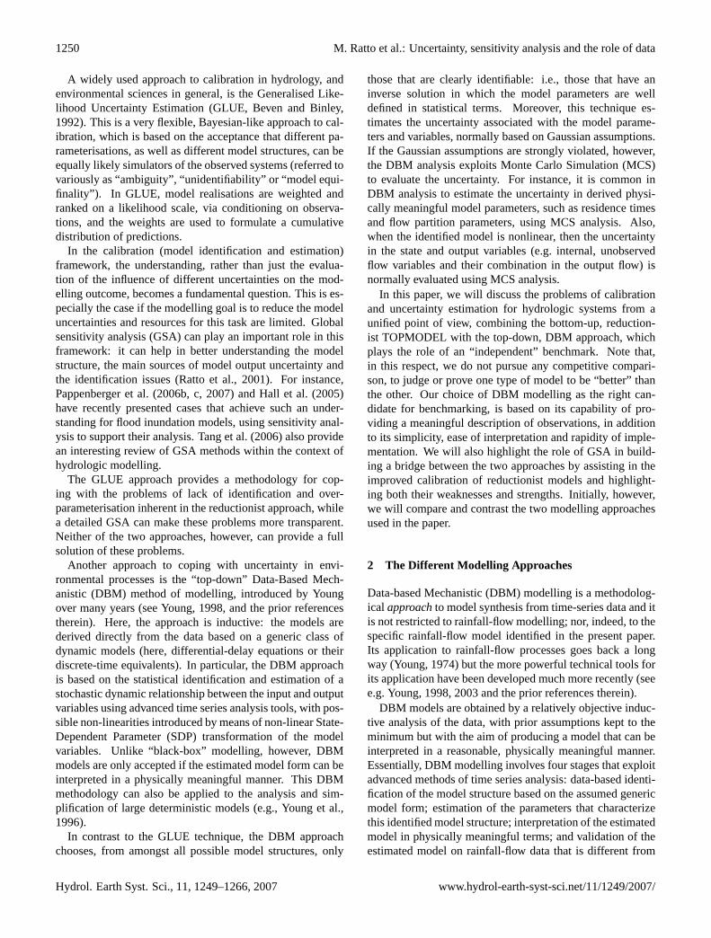
The data set used in this example contains hourly data forrainfall, evaporation and flow observations for the River Hod-der at Hodder Place, North West England, 1991. The RiverHodder has a catchment area of 261 km2 and it forms part ofthe larger River Ribble catchment area of 456 km2. The Hod-der rises in the Bowland Fells and drains a thinly populated,entirely rural catchment and, together with the River Calder,it joins the River Ribble just downstream of a flow gaugingstation at Henthorn. There is a reservoir in the catchmentwhich alters the water regime on a seasonal basis.

Data from the Hodder catchment have been analysed be-fore using DBM modelling: first, with the objective of adap-tive forecasting, using the flow measurement as a surrogatefor catchment storage (Young, 2002); and second, as a simu-lation model (Young, 2003), where the catchment storage ismodelled as a first order dynamic system with rainfall as theonly input. In both cases the data set used is quite short: itconsists of 720 and 480 hourly samples, respectively, withthe rainfall series based on the Thiessen polygon averageof 3 tipping bucket rain gauges. Based on these data, thelatter model, in particular, achieves excellent validation per-formance, with the model output explaining 94% of the ob-served flow, only marginally less than the 95% achieved incalibration.

In the present example, we have chosen a data set that issomewhat longer, with 1200 hourly samples, but the rain-fall measurements are from a single rain gauge. Probablyas a result of this and other inconsistencies in the data dueto a reservoir operation (see later discussion in Sect. 4.1),the rainfall-flow data used for calibration and validation ex-hibit some problems from a modelling standpoint and, as weshall see, the validation performance of both the DBM modeland TOPMODEL is considerably worse than that achievedin the previous DBM modelling studies. However, this has

the virtue of allowing us to see how the modelling method-ologies function when confronted with data deficiency andhow our proposed combined approach, involving GSA, canprovide useful results, even when using relatively poor datasuch as these, which are similar to those often experienced inpractical hydrological applications.

Only the rainfall-flow data are used in the DBM mod-elling; while the TOPMODEL calibration uses the DTMand evaporation data, in addition to the rainfall-flow mea-surements. The January–March 1991 rainfall-flow data areused for the identification and estimation (calibration) ofboth models; while the second part of the data (October–December) is used for the validation. The catchment is pre-dominantly covered by grassland and, during summer time,the flow is affected by abstractions from the reservoir situ-ated in the catchment. Therefore, for simplicity and to makethe model comparisons more transparent, it will be noted thatonly Autumn–Winter months are used for the modelling. Ofcourse, both models would require further evaluation, basedon a much more comprehensive data set, before being usedin practice.

4.1 DBM rainfall-flow model for Hodder catchment

Following the DBM modelling procedure outlined in Sect. 2,the first model structure identification stage of the modellingconfirms previous research and suggests that the only signif-icant SDP nonlinearity is associated with the rainfall input.This “effective rainfall” nonlinearity is identified from thedata in the following form:

uet = f (yt ) × rt

whereuet denotes effective rainfall,rt denotes rainfall andf (yt ) denotes an estimated non-parametric (graphical) SDPfunction in which, as pointed out in Sect. 2, the flowyt is act-ing as a surrogate for the soil moisture content in the catch-ment (catchment storage).

The non-parametric estimate of the state-dependent func-tion f (yt ) is plotted as the full line in Fig. 1, with the stan-dard error bounds shown dotted. The shape of the graphicalSDP function suggests that it can be parameterised as eithera power law or an exponential growth relationship. However,in accordance with previous research (see above references),the more parsimonious power law relationshipf (yt )=g y

βt

is selected for the subsequent “parametric estimation” stageof the DBM modelling, whereg is a scale factor selected tomake the the SDP coefficientf (yt )=1.0 at maximum flow.

The best identified linear STF model between the effectiverainfall uet=g y

βt ×rt and flow is denoted by the usual triad,

as [2 2 0]; i.e. a TF model with 2nd order denominator, 2ndorder numerator and no advective time delay. This results in



0 0.5 1 1.5 2 2.5 3

x 10−3

−0.4

−0.2

0

0.2

0.4

0.6

0.8

1

1.2

Flow (acting as surrogate for catchment storage)

Sta

te D

epen

dent

Par

amet

er e

stim

ate

Fig. 1. This graph shows the estimated non-parametric SDP rela-tionship (full line) between measured flow and the effective rainfallparameter, where the flow is acting as a surrogate for catchment soilmoisture. The 95% confidence bands are shown by the dotted linesand the dash-dot line is a parametric estimate of the SDP relation-ship obtained in the later estimation stage of the modelling using apower law approximation.

the following, nonlinear DBM model between the rainfallrtand flowyt :

uet = 10.258y0.411t × rt

x̂t =

[0.0045

1−0.9903z−1 +0.1269

0.86821z−1

]uet

yt = x̂t + ξt ; var(ξt ) = 0.042x̂2t

(8)

whereξt represents the estimated noise on the relationshipwhich, as shown, is modelled as a (state-dependent) het-eroscedastic process with variance proportional to the squareof the estimated flow,̂x2

t , andz−1 is the backward shift oper-ator: i.e.z−syt=yt−s .

Concerning the expressionuet=f (yt )×rt , it is worth not-ing that, in its present, purely surrogate role, the flow seriesis not being used as an additional input to the model (i.e. inaddition to the rainfall) in the normal sense: rather, at eachtime point, it simply affects the value of the state-dependentgain coefficientf (yt ) that multiplies the rainfall in its con-version to effective rainfall. Therefore, no dynamic systemis involved as there would be if one used the modelled flowrather than the measured flow in this equation. The resultingeffective rainfall occurs on the same time point as the realrainfall and just the level of rainfall at this time is changed.In other words,no flow feedbackoccurs at all in the model.

However, this exploitation of the flow measurement as asurrogate measure of soil moisture content in the catchmentdoes restrict the present model’s use to defining the dom-inant dynamic characteristics of the catchment, as well asfor data assimilation and flow forecasting applications. Itcannot be used for simulation, although an alternative DBM

0 200 400 600 800 1000 12000

1

2

3x 10

−3

slow

com

pone

nt [m

/h]

0 200 400 600 800 1000 12000

1

2

3x 10

−3

fast

com

pone

nt [m

/h]

time [h]

Fig. 2. The estimated slow (upper panel) and quick (lower panel)flow components of the DBM model output. The most likely in-terpretation of these component flows is that the slow componentrepresents the “groundwater” (baseflow) effects and the quick com-ponent represents the “surface and near-surface” process effects.

simulation model has been developed by introducing a parsi-monious model for catchment storagest (e.g. Young, 2003).This replaces the flowyt in the above definition ofuet , and,if required, a similar model could involve temperature and/orevapo-transpiration data, when these are available (see e.g.the rainfall-flow models developed by Whitehead and Young,1975; Jakeman et al., 1990).

The noiseξt identified in DBM modelling represents thatpart of the data not explained by the model. It can be quan-tified in various ways: e.g. simply by its variance; by itsvariance in relation to that of the model output; by a het-eroscedastic process, where the variance is modulated insome state-dependent manner, as in the present paper; by acoefficient of determination; by a stochastic model, if such amodel is applicable; by its probability distribution; or by itsspectral properties. Of course, it can be due to various rea-sons: measurement inaccuracies, limitations in the model asa representation of the data, the effects of unmeasured inputs,etc. Sometimes, if it has rational spectral density, this noisecan be modelled stochastically, e.g. by an Auto-Regressive(AR) or an AutoRegressive, Moving Average (ARMA) pro-cess, but this is not always applicable when dealing with realdata (see later). Consequently, the “instrumental variable”identification and estimation methods used for DBM mod-elling are robust in the face of noise that does not satisfy suchassumptions (see e.g. Young, 1984).

In order to reveal the most likely mechanistic interpreta-tion of the model, the [2 2 0] STF relationship in the model(8) is decomposed by objective continued fraction expan-sion (calculus of residues) into a parallel form that revealsthe major identified flow pathways in the rainfall-flow sys-tem: namely, a “slow” component whose flow response isshown in the upper panel of Fig. 2, with a residence time(time constant) equal to 103 h; and a “quick” flow compo-nent, with a residence time of 7.1 h, whose flow response is



Table 1. Synthetic table of main calibration and validation results.

CalibrationR2T

ValidationR2T

DBM 0.928 0.79DBM (CT) 0.917 0.838TOPMODEL (base) 0.905 0.747TOPMODEL (pre-calib.)

case (a) 0.883 0.766case (b) 0.880 0.762case (c) 0.53 < 0

shown in the lower panel of Fig. 2. However, it should benoted that, while the quick residence time is estimated well,with narrow uncertainty bounds (95 percentile range between7.2 h and 6.9 h), the slow residence time is poorly estimatedwith a skew distribution (95 percentile range between 81 hand 136 h). This is due to the residence time being relativelylarge in relation to the observation interval of 1200 h, so thatthe information in the data on this slow mode of behaviour israther low.

The partition of flow between these quick and the slowcomponents, respectively, is identified from the decomposedmodel with about 68% of the total flow appearing to arrivequickly from surface and near surface processes; while about32% appears as the slow-flow component, probably due, atleast in part, to the displacement of groundwater into theriver channel (base flow). The decomposition and its asso-ciated partitioning are a natural mathematical decompositionof the estimated model which has a nice interpretation inboth dynamic systems and in hydrological terms (see e.g.Young, 2005). It is a function of two mathematical prop-erties of model: the eigenvalues, which define the residencetimes of the “stores” in the parallel pathways; and the steadystate gains of these stores, that define how much flow passesthrough each store1. However, it must be emphasised that theuncertainty associated with the partitioning in this particularexample is high because of the uncertainty in the estimationof the slow residence time.

It is clear from this analysis that the partitioning of theDBM model, as identified in this manner, is inferred fromthe data by the DBM modelling methodology and it is notimposed on the model in any way by the modeller, as inother approaches to rainfall-flow modelling. For example,the interested reader might compare the HyMOD model ofMoradkhani et al. (2005) of the Leaf River, where the modelstructure is assumed by the modellers, with the DBM modelof Young (2006), which is based on the same data set butwhere a similar but subtly different structure is inferred fromthe data.

1Another feedback decomposition is possible (identifiable) butthis is rejected because it has no clear physical interpretation.

0 100 200 300 400 500 600 700 8000

0.5

1

1.5

2

2.5

3x 10

−3

time [h]

flow

[m/h

]

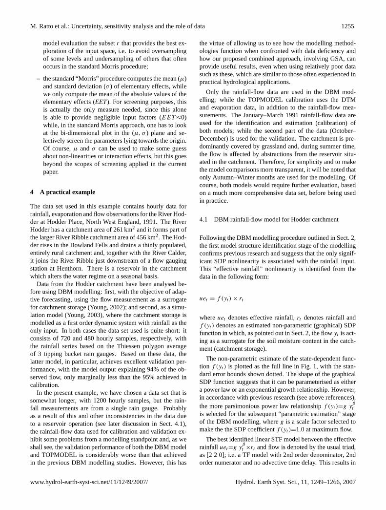
Fig. 3. Validation of the DBM model on October–November 1991period, 79% of output variation explained; dots denote the obser-vations, simulations are marked by a solid black line, shaded areadenotes 95% confidence bands.

In Table 1, the main results in calibration and valida-tion for the DBM model and TOPMODEL are synthesised.The DBM model (8) has a Coefficient of Determination,R2

T =0.928 (i.e. 92.8% of the measured flow variance is ex-plained by the simulated model output), which is a sub-stantial improvement on the linear model (R2

T =0.84), whereit involves the addition of the single power law parameter.Clearly, the use of observed flow in the definition of effec-tive rainfall feeds some information about output flow in thelinear STF (see earlier discussion). However, similar per-formance is obtained when the catchment storagest is mod-elled from rainfall data, without any use of flow data (Young,2003). This confirms that it is a sensible identification ofthe input nonlinearity and its associated effective rainfall thatallows the model to describe well the observed system, notthe use of flow data per se. Finally, the estimated noiseξt isidentified as a heteroscedastic, high order process.

Note that we have not carried out any Monte Carlo Simula-tion (MCS) analysis in connection with the model (8), in or-der to emphasise that this is not essential in DBM modelling:the 95% confidence bands, as shown later in Fig. 3, for ex-ample, are a function of both the estimated parametric un-certainty and the residual heteroscedastic noiseξt . Withoutthe MCS analysis, the DBM modelling is very computation-ally efficient, normally involving only a very small computa-tional cost (a few seconds of computer time). This contrastswith the TOPMODEL analysis, considered in the next sec-tion, where computationally much more demanding MonteCarlo Simulation analysis is an essential aspect of the GLUEcalibration and uncertainty analysis. Consequently, it is easyto use the DBM modelling for the role suggested in this pa-per.



Table 2. Parameter distributions applied in MC calibration of TOPMODEL.For each parameter, the top line shows the ranges for the base calibration exercise, while modified ranges for pre-calibration cases (a,b,c) arespecified, when applicable.

Parameters Distribution Min. Max. Mean Std

input uniform 0.8 1.2 1 0.116case (c) uniform 0.8 1 0.9 0.0577

SK0 uniform 10 000 40 000 25 000 8600

m uniform 0.001 0.03 0.0157 0.008cases (a, b) uniform 0.005 0.03 0.0175 0.0072case (c) uniform 0.0025 0.003 0.00275 1.44e-4

LRZ uniform 1.e-4 0.04 0.02 0.012case (c) uniform 0.015 0.04 0.0275 0.0072

KS log-uniform 1.e-7 1.e-3 1.08e-4 2.05e-4case (c) log-uniform 1.e-4 1.e-3 3.9e-4 2.49e-4

δ uniform 0.001 0.2 0.1 0.0575case (a) uniform 0.01 0.2 0.105 0.0548case (b) fix 0.15 0.15 - -case (c) uniform 0.1 0.2 0.15 0.0289

Quite often, however, MCS analysis is used as an ad-junct to DBM modelling, in order to evaluate various ad-ditional aspects of the model: e.g. the uncertainty associ-ated with the “derived parameters”, e.g., the residence timesand partitioning percentages of the decomposed model (seee.g. Young, 1999), as well as the effects of stochastic inputnoise. Typically, the uncertainty associated with the DBMflow response is mainly accounted for by model output error,which in DBM modelling is considered as output “measure-ment noise” (see earlier).

The model validation results are shown in Fig. 3 and Ta-ble 1: here only 79.0% of measured flow variation is ex-plained by the DBM model. This is a little better than TOP-MODEL which explains 74.7% of the output variation (seelater Sect. 4.2). Interestingly, the performance of the DBMmodel is improved if the continuous-time (CT) version ofthe model (see e.g. Young, 2005) is identified and estimatedusing the continuous time version (RIVC) of the RIV algo-rithm in the CAPTAIN Toolbox. Although the calibrationR2

T =0.917 is then marginally less than for the discrete-timeDBM model, the validationR2

T =0.838 is improved.

The main difference between the models is that the DBMmodel validates well on the peak flows, while TOPMODELdoes not do so well in this regard, although having somewhatbetter performance than the DBM model at lower flows. Bothof these results are not particularly good, however, in com-parison with previous DBM rainfall-flow modelling resultsbased on Hodder data (see previous discussion), where 94%of the output variation is explained by the model during val-idation. It is also worse than other typical DBM modellingresults (see the cited references on DBM modelling), where

85–95% of the flow is normally explained by the model dur-ing validation.

As pointed out previously, this poor performance is almostcertainly due to data deficiencies in the form of poor, sin-gle gauge rainfall observations and other inconsistencies inthe flow measurements arising from the reservoir operations.Note that, in this example, the high level of uncertainty of theslow flow component (see earlier comments) has a deleteri-ous effect on the validation performance of the DBM modelbecause the validation error is particularly sensitive to errorsin this slow flow component. Also, it is interesting to notethat, if the DBM model calibration is performed on the val-idation data set, only 84% of flow variation is explained bythe model with the same structure. Compared with this, theabove validation figures (79.0% and 74.7%) are not as badas they look at first sight. However, this reinforces our com-ments about the deficiences in the data, particularly, it wouldappear, the validation data set.

Despite these limitations in the data, the modelling re-sults are satisfactory for the illustrative purpose of the presentpaper (i.e. presentation of the two different approaches torainfall-flow modelling and how they may be combined)since both models are subject to exactly the same data defi-ciency and the results reveal interesting comparative aspectsof the models.

4.2 TOPMODEL calibration for Hodder catchment

In the present context, the main aim of the TOPMODEL(Beven and Kirkby, 1979) is the estimation of the uncertaintyassociated with the flow predictions for the Hodder catch-ment, using the same data as those used in the previous sec-



tion. The choice of TOPMODEL is justified by its simplestructure and its mechanistic interpretation: it has a total of9 parameters but only 4 of these are considered in the cali-bration and the associated sensitivity analysis described here,in addition to uncertainties pertaining to the input and outputobservations. TOPMODEL bases its calculations of the spa-tial patterns of the hydrological response on the pattern of atopographic index for the catchment, as derived from a Dig-ital Terrain Model (DTM). We have chosen the SIMULINKversion of TOPMODEL, described in Romanowicz (1997),because of its clear, modular structure. This model has al-ready been applied in similar Monte Carlo settings by Ro-manowicz and Macdonald (2005). The saturated zone modelis assumed to be nonlinear, with the outflowQb(t) calcu-lated as an exponential function of a catchment average soilmoisture deficitS, i.e.,

dS(t)

dt= Qb(t) − Qv(t) Qb(t) = Q0 exp(−S(t)/m) (9)

whereQ0=SK0 exp(−λ) is the flow whenS(t)=0; Qv(t)

denotes the recharge to the saturated zone;SK0 is a soiltransmissivity parameter;m is a parameter controlling therate of decline in transmissivity with increasing soil moisturedeficit; andλ is the mean value of the topographic index dis-tribution in the catchment (Beven and Kirkby, 1979). Otherparameters control the maximum storage available in the rootzone (LRZ) and the rate of recharge to the saturated zone(KS). The calibration exercise includes the analysis of un-certainties associated with the input and output observations(i.e., rainfall and flow), the model structure and its parame-ters.

We assume here that rainfall observations are affected by abiased measurement, accounted for by a multiplicative noise(input in Table 2) of±20% that is applied to rainfall data ateach Monte Carlo Simulation (MCS) run. Flow observationuncertainty is included in the choice of the error model struc-ture, which is assumed to follow a fuzzy trapezoidal member-ship function (for a similar application see Pappenberger andBeven, 2004). The breakpoints of the trapezoid are given bythe array[A, B,C, D] = [1−4δ, 1−δ, 1+δ, 1+4δ], whereδ

denotes the characteristic width of the trapezoid. Breakpointsfor each time location are determined by multiplication e.g.for theA breakpoint at timet , At=yt (1−4δ), implying a het-eroscedastic error structure. The widthδ of the trapezoidalmembership function is assumed to be uncertain as well, ina range between [0.1% and 20%]. This will allow the sen-sitivity of the calibration to the assumptions about the errormagnitude to be evaluated.

Parameter uncertainty is taken care of in the choice of theparameter ranges for the parametersSK0, m, LRZ, KS, as re-quired for the MCS analysis. The influence of the modelstructure uncertainty may be accounted for via a randomsample from different model structures (e.g., TOPMODELwith and without dynamic contributing areas). In this paper,

we restrict the analysis to parametric and observational un-certainty.

To some extent and in contrast to the DBM modelling, thespecification of the above uncertainty on the input parame-ters, as required for the MCS analysis, is subjective and willdepend upon the experience and prior knowledge of the ana-lyst. Consequently, these specifications may well be adjustedfollowing the investigation of the initial MCS results, as dis-cussed later.

In this example, the MCS analysis involves 1024 runs ofTOPMODEL, sampling parameters from the ranges spec-ified in Table 2 using quasi-random LPTAU sequences(Sobol’ et al., 1992). The sample size requirements of GLUEapplications are mainly linked to the convergence of the cu-mulative distribution functions (Pappenberger et al., 2005;Saltelli et al., 2004, p. 153–155) and thus to the “successrate”, i.e. the percentage of samples that provides good fit.Given the relatively small number of parameters in this case,the sample size was sufficient for the current application.Moreover, we also kept the computational cost at the mini-mum to show that careful pre-calibration based on sensitivityanalysis results allows for a reduction of the computationalcosts of GLUE exercises, by improving the “success rate”(see Sect. 4.2.1 below).

In the GLUE approach, the predictive probability of theflow takes the form:

P(x̂t < y|�) =

∑{i:x̂t<y|ϑi ,�}

f (ϑi |�) (10)

wherex̂t are simulated outputs andf (·) denotes the likeli-hood weight of parameter sets2= {ϑ1, ..., ϑn}, in which n

is the number of MC samples, conditioned on the availableobservations� = {y1, . . ., yT }.

The next step is to investigate the weights. The trapezoidalmembership function, at each discrete timet and each ele-mentϑi , i=1, ...n of the MC sample, takes the values:

ft (ϑi |yt ) = 1 if Bt < x̂t < Ct

ft (ϑi |yt ) =x̂t−At

Bt−Atif At < x̂t < Bt

ft (ϑi |yt ) =x̂t−Dt

Ct−Dtif Ct < x̂t < Dt

ft (ϑi |yt ) = 0 if x̂t < At , x̂t > Dt

(11)

where At=yt (1−4δi), Bt=yt (1−δi), Ct=yt (1+δi),Dt=yt (1+4δi). The likelihood weight for each parameterset is, therefore:

f (ϑi |�) ∼

T∑t=1

ft (ϑi |yt ) (12)

In the present case study, the confidence bounds resultingfrom the GLUE methodology will depend on the widthδ ofthe trapezoidal membership function. This function giveszero weight for the simulations falling outside the rangeyt (1±4δ) at any time (i.e. outside a relative error bound of400δ%); while it will be maximum for those falling within



0 100 200 300 400 500 600 700 800 9000

1

2

3

4

5

6

7x 10

−3

time [h]

flow

[m]

Fig. 4. Validation of the TOPMODEL: 74.7% of output varia-tion explained; dots denote the observations, simulations (posteriormean) are marked by a solid black line, shaded area denotes 95%confidence bands.

the rangeyt (1±δ) at any time (i.e. within a relative errorbound of 100δ%). The values ofδ used in the MCS (Ta-ble 2) range from a very strict rejection criterion (simula-tions are rejected if the relative error at any time is larger than±0.4%) to a very mild one (simulations are given the max-imum weight when the relative error at any time is smallerthan±20%, while they are rejected only when they fall out-side the±80% bound). This initially wide range will un-dergo a revision in the second part of this example, based onsensitivity analysis results and taking DBM uncertainty es-timation as a benchmark for adjusting (pre-calibrating) thepriors in a less subjective way than this initial set-up. How-ever, as discussed later,δ is not the only parameter stronglydriving the uncertainty bounds, withm playing an importantrole as well.

The calibration flow predictions of TOPMODEL explain90.5% of the observed flow variations (see Table 1), not sig-nificantly different from that obtained using the DBM ap-proach (92.8%). Note that TOPMODEL utilises evaporationmeasurements in addition to the rainfall and flow measure-ments used in the DBM model. The model residuals areheteroscedastic and highly coloured, even more so than theDBM model residuals. On the validation data (Fig. 4), themodel output explains 74.7% of the flow variations, a littleworse than DBM (79.0%: see Fig. 3). On the other hand,looking at the results in more detail, two major differencesappear:

1. The 95% uncertainty bound of the calibrated TOP-MODEL at the peak flows is about twice the bound ofthe DBM model. The latter uncertainty bounds seemmore reasonable, given the nature of the observationsaround the peak flows.

0 200 400 600 800 1000 12000

2

4

6

8

10

Sat

. & g

roun

dwat

. fl.

[m]

0 200 400 600 800 1000 12000

1

2

3

4

5x 10

−3

time [h]

Sur

f. ru

noff

[m]

x 10−3

x 10−3

Fig. 5. Uncertainty estimation of the discharge from the satu-rated subsurface store (upper panel) and of the “surface runoff”(lower panel) of the TOPMODEL; simulations (posterior mean) aremarked by a solid black line, shaded area denotes 95% confidencebands.

2. The partition of the output flow of the TOPMODEL intotwo components, deriving from rainfall on the dynamicsaturated contributing areas (denoted here as “surfacerunoff”) and from the discharge from a nonlinear sat-urated subsurface store, differs from the DBM’s parti-tioning, as discussed previously, and is shown in Fig. 5.The saturated contributing area accounts for only 5%of the predicted discharge, with “quick” dynamical fea-tures merely adjusting the flow peaks, while the remain-der is contributed by the nonlinear subsurface store.

4.2.1 Sensitivity analysis: is it possible to reduce volatilityof predictions?

As discussed in Sect. 3, sensitivity analysis can play a keyrole in model calibration. We have seen that the uncertaintyfrom the calibrated TOPMODEL is much larger than for theDBM model (notice the difference in the vertical axis scalesof the figures caused by this). Taking DBM as a relativelyobjective benchmark for uncertainty estimation, we wouldlike to analyse under which conditions the volatility of pre-dictions can be reasonably reduced. This is a typical examplefor the Factors Prioritisation setting, where one can identifystrategies for the reduction of the uncertainties of the TOP-MODEL, acting on the parameters having the highest maineffects. To do so, we perform the sensitivity analysis for thelikelihood weights (Ratto et al., 2001).

In Table 3, first column, we show the main effect indices,computed on the same 1024 runs used for calibration and ap-plying the State Dependent Regression method by Ratto etal. (2004, 2006); while in Table 3, second column we showthe Elementary Effect Test (EET), computed using only anadditional 168 model runs. The main effects tell us that the



0.8 1 1.20

200

400

600

800

1000

1200Input

0 0.01 0.02 0.030

200

400

600

800

1000

1200m

1 2 3 4

x 104

0

200

400

600

800

1000

1200sko

0 0.02 0.040

200

400

600

800

1000

1200LRZ

10−7

10−5

10−3

0

200

400

600

800

1000

1200KS

0 0.1 0.20

200

400

600

800

1000

1200δ

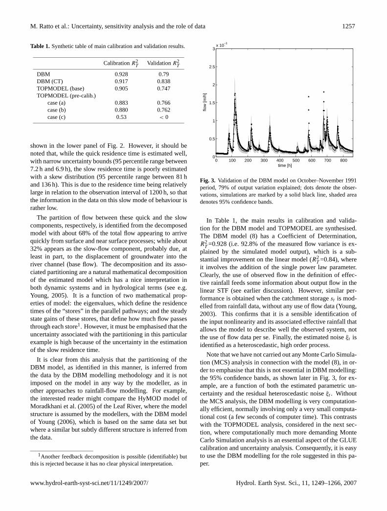
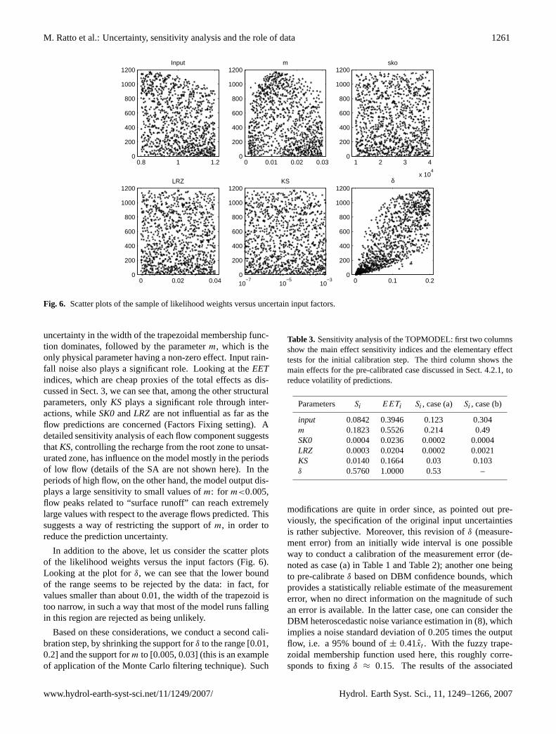
Fig. 6. Scatter plots of the sample of likelihood weights versus uncertain input factors.

uncertainty in the width of the trapezoidal membership func-tion dominates, followed by the parameterm, which is theonly physical parameter having a non-zero effect. Input rain-fall noise also plays a significant role. Looking at theEETindices, which are cheap proxies of the total effects as dis-cussed in Sect. 3, we can see that, among the other structuralparameters, onlyKS plays a significant role through inter-actions, whileSK0andLRZ are not influential as far as theflow predictions are concerned (Factors Fixing setting). Adetailed sensitivity analysis of each flow component suggeststhatKS, controlling the recharge from the root zone to unsat-urated zone, has influence on the model mostly in the periodsof low flow (details of the SA are not shown here). In theperiods of high flow, on the other hand, the model output dis-plays a large sensitivity to small values ofm: for m<0.005,flow peaks related to “surface runoff” can reach extremelylarge values with respect to the average flows predicted. Thissuggests a way of restricting the support ofm, in order toreduce the prediction uncertainty.

In addition to the above, let us consider the scatter plotsof the likelihood weights versus the input factors (Fig. 6).Looking at the plot forδ, we can see that the lower boundof the range seems to be rejected by the data: in fact, forvalues smaller than about 0.01, the width of the trapezoid istoo narrow, in such a way that most of the model runs fallingin this region are rejected as being unlikely.

Based on these considerations, we conduct a second cali-bration step, by shrinking the support forδ to the range [0.01,0.2] and the support form to [0.005, 0.03] (this is an exampleof application of the Monte Carlo filtering technique). Such

Table 3. Sensitivity analysis of the TOPMODEL: first two columnsshow the main effect sensitivity indices and the elementary effecttests for the initial calibration step. The third column shows themain effects for the pre-calibrated case discussed in Sect. 4.2.1, toreduce volatility of predictions.

Parameters Si EETi Si , case (a) Si , case (b)

input 0.0842 0.3946 0.123 0.304m 0.1823 0.5526 0.214 0.49SK0 0.0004 0.0236 0.0002 0.0004LRZ 0.0003 0.0204 0.0002 0.0021KS 0.0140 0.1664 0.03 0.103δ 0.5760 1.0000 0.53 –

modifications are quite in order since, as pointed out pre-viously, the specification of the original input uncertaintiesis rather subjective. Moreover, this revision ofδ (measure-ment error) from an initially wide interval is one possibleway to conduct a calibration of the measurement error (de-noted as case (a) in Table 1 and Table 2); another one beingto pre-calibrateδ based on DBM confidence bounds, whichprovides a statistically reliable estimate of the measurementerror, when no direct information on the magnitude of suchan error is available. In the latter case, one can consider theDBM heteroscedastic noise variance estimation in (8), whichimplies a noise standard deviation of 0.205 times the outputflow, i.e. a 95% bound of± 0.41x̂t . With the fuzzy trape-zoidal membership function used here, this roughly corre-sponds to fixingδ ≈ 0.15. The results of the associated



0 100 200 300 400 500 600 700 800 9000

0.5

1

1.5

2

2.5

3

x 10−3

time [h]

flow

[m]

Fig. 7. Revised validation of the TOPMODEL, to reduce volatilityof predictions, case (a): 76.6% of output variation explained; dotsdenote the observations, simulations (posterior mean) are markedby a solid black line, shaded area denotes 95% confidence bands.Surface flow partition: 3.5% of the overall flow.

calibration and validation exercises are denoted as case (b)in Table 1 and Table 2 .

Figure 7 shows the updated validation exercise for case (a):the portion of flow variance now explained by the new cali-brated model is 88.3% (Table 1), only slightly less than in theinitial setting. The uncertainty bound is now comparable tothe one obtained in the DBM analysis, i.e. we have managedto obtain less volatile model predictions. How significantlydoes this affect the fitting performance? In the present step,10.4% of the data fall outside the 95% bound, whereas thiswas 4.7% for the previous case. This is exclusively due to alarger number of time periods where the model uncertaintybound is above the data, so the results are on the “safe” side.

The partitioning is also hardly modified: “surface runoff”is now 4.3% of the overall flow. Cutting the high tails fromthe uncertainty distribution of surface runoff flows did notalter the partitioning too much, meaning that the high tailsin the upper panel of Fig. 5 are not supported by the data.The validation step confirms the results (Table 1): 76.6% ofthe data is now explained by model predictions, i.e. a slightlylarger amount than before. Although this is not a statisticallysignificant improvement, there is clearly no degradation inthe results, and this is an indication of the validity of the ap-proach proposed in this paper. The uncertainty bounds in thiscase are also similar to DBM, with the drawback of a largerportion of data below the bounds in periods of small flow:14.3% versus the 6.4% of the initial case.

The calibration/validaton results for case (b) are almostidentical to case (a) (see Table 1). This shows that, usingDBM results for the GLUE calibration, can allow for the cal-ibration of the measurement error in a reasonable manner,thus reducing the number of uncertain parameters.

In both of these new calibration steps, the effect of thedifferent uncertainty sources is different. For case (a),δ re-mains the most important parameter, but its sensitivity de-creases, while the sensitivity ofm increases. Moreover,KSalso acquires a small main effect (see Table 3, third col-umn). For case (b), on the other hand, we can see that fix-ing δ based on DBM estimation allows other sensitivity pat-terns to be revealed more clearly and in a more balancedway, and balanced main effects are usually a sign of betteridentification. In particular, we have that, among the struc-tural parameters,bothm andKShave a significant effect onmodel performance. Lack of identification is still presentfor SK0 and LRZ, however, which can have virtually anyvalue in their prescribed prior ranges without significantlyaffecting the model performance in predicting outflow (over-parameterisation or equifinality). This is an example of whatis called, in sensitivity analysis, “fit for purpose”. We actu-ally know that both of these parameters should have an effecton flow, as they show threshold-like behaviour (Romanowiczand Beven, 2006). However, this behaviour has no significantimpact on the fit of observations for the current case study,implying the irrelevance ofSK0andLRZ for the purposes ofoutflow predictions. Of course, this is not a general result: itdoes not mean that there are not other “behavioural” classifi-cations or other data sets that may highlight the role ofSK0andLRZ.

4.2.2 Sensitivity analysis: is other partitioning possible?

As pointed out previously, the interpretation of the partition-ing and decomposed flows of rainfall-flow models is opento subjective judgement and it is expected that the partition-ing of the two models will be different because it is con-strained in TOPMODEL by the assumptions built into itsformulation, namely by the surface contributing areas. Con-sequently, TOPMODEL’s decomposition may not be consid-ered any less physically acceptable than the one suggested bythe DBM model. However, the relatively objective nature ofthe DBM analysis and its association of the partitioning withthe estimated steady state gains and residence times of theDBM model is persuasive and, we believe, provides a veryreasonable decomposition (although this is likely to dependon the view of the hydrologist and not all readers will agree).For instance, if we consider the observed flow response, thereseems to be an appreciable base-flow component and theDBM model estimate of the “slow-flow” component seemsconsistent with what one might expect in this regard. On theother hand, TOPMODEL’s partitioning, based on predictedcontributing areas, gives quite a different form of partition-ing, with part of the fast response provided by the nonlinearsubsurface store. Consequently, purely as an illustrative ex-ercise, it might be instructive to use sensitivity analysis toinvestigate whether other partitions are possible within theuncertainty specifications of the TOPMODEL. This helps tofurther demonstrate how GSA can assist in model evaluation



and in revealing the essential differences between differentmodel mechanisms. In particular, this will exemplify the ca-pability of MCF techniques in constraining models into spec-ified behavioural characteristics,if this is desirableaccordingto the modeller’s views. This exercise is, in practice, the dualto that considered in the previous section.

The MCF procedure adopted for this purpose was to targetmore balanced partitioning, starting from the base MC sam-ple used in Sect. 4.2, i.e., in this case, the behavioural clas-sification requires higher portion of surface runoff,irrespec-tive (initially) of the implications this may have on the modelfit. This MCF analysis shows that the portion of surface flowcan be increased to 30–40% only for very small values ofm. Remembering the results in previous Sections, this turnsout to be the range ofm values displaying the smallest GLUEfuzzy weights, as well as the complementary support adoptedto reduce the uncertainty of TOPMODEL predictions. Thisalready anticipates that, while it is possible to change the par-titioning in TOPMODEL, this may be rejected by a reducedability of the model to explain the data. Nonetheless, we at-tempted to calibrate the TOPMODEL by restrictingm in therange [0.001–0.003], to verify that there are not other fea-tures in TOPMODEL that allow the model to fit the data insuch a constrained situation. The calibration failed, with 93%of MC runs having negativeR2

T values and huge uncertaintybands. This considered, we tried a final MCF step, in whichwe kept only the 7% runs with positiveR2

T (denoted as case(c) in Table 1 and Table 2). This strategy resulted in an un-satisfactoryR2

T =53% in calibration, with the contribution ofsurface flow in the range 10–20%. The confidence boundson the flow response are narrower than in the previous cali-brations, with a large part of flow under-predicted in periodsof low flow; while the flow peaks tend to be over-predicted.Also, the dynamical features of the two flow components ofthe model still appear too similar: both of them present clearrapid response to rainfall episodes and increasing the “sur-face” component, also makes the response of the “subsur-face” flow larger. Finally, the validation results are totallyunacceptable (R2

T <0).The above analysis provides an instructive academic ex-

ample of how MCF techniques can be used to investigatewhether the parameters of a mathematical model can be mod-ified to yield specific behavioural characteristics (partitioningin this case). However, for the present TOPMODEL case-study this severely impairs the model’s ability to explain theobserved data. As a result, and not surprisingly given the na-ture of TOPMODEL, the partitioning objective fails and thepossibility of changing the model behaviour in this sense isrejected.

5 Discussion

This paper has described a modelling framework for rainfall-flow modelling that combines bottom-up, reductionist mod-

elling with top-down, parsimonious modelling. This com-bined approach, which exploits sensitivity analysis to builda bridge between the two types of model, has been illus-trated by its application to intentionally selected poor datafrom the Hodder catchment in the North West of England,using the physically based, semi-distributed rainfall-runoffmodel TOPMODEL to exemplify the bottom-up approach;and DBM modelling to exemplify the top-down alternative.

The DBM model yields a well identified representation ofthe Hodder data, with good (92.8%) explanation of the flowdata in calibration, as well as a clear mechanistic interpreta-tion arising from the identified linear, second order stochas-tic transfer function between effective rainfall and outputflow. In particular, the output flow of the DBM model canbe further decomposed into a “slow” (32.3%) and a “quick”(67.7%) component, with a suggested physical interpreta-tion that these are associated with “groundwater” and “sur-face/near surface” processes, respectively. In terms of ex-plaining the flow data, the calibration results from the TOP-MODEL analysis are not all that different from those of theDBM model but the flow decomposition is much different(see below). As expected from the data-set chosen, the vali-dation results for both models are not particularly good, withthe DBM model explaining 79% of the validation flow vari-ation and TOPMODEL yielding a little less than this, almostcertainly because of the data deficiences mentioned aboveand discussed in Section 4 of the paper.

Two issues arise from the initial sensitivity analysis ofTOPMODEL (i.e. with the initially specified nominal param-eters and uncertainty bounds) that reveal potentially impor-tant differences between the stochastic and dynamic char-acteristics of the TOPMODEL and the DBM model. First,the large volatility of TOPMODEL predictions, with confi-dence bounds twice that of the DBM model; and second,the behaviour of the two output flow components in theTOPMODEL, with the subsurface component accounting formost of the output flow, while the surface component hascomparatively little impact on the model output flow.

As regards the high volatility of the TOPMODEL predic-tions, GSA shows that less volatile performance is possible,without significantly affecting the explanation of the data(the R2

T slightly improves while the data are below confi-dence bounds for a larger number of time periods), by actingon the prior supports of the two most relevant parameters:m

andδ. This also shows how the combined use of DBM andGSA results can be helpful for model identification and sim-plification: (i) whenδ is fixed according to DBM estimation(case (b)), identification ofm andKS is strongly enhanced;(ii) SK0 is clearly highlighted as irrelevant for calibrationpurposes and, hence, it can be fixed at a nominal value. Inrelation to flow partitioning, GSA confirms that it is impos-sible to bring the two models into reasonable agreement asregards the flow partitioning, which is not all that surpris-ing since the models have significant structural differences:DBM’s inference is based ondynamicalfeatures identified



from the data, like residence times; while TOPMODEL’s isbased on the concept of dynamic contributing areas inspace.

One of these differences lies in the nature of the nonlin-earity. As in the present example, the application of the rela-tively objective State-Dependent Parameter (SDP) estimationprocedure to other rainfall-flow data considered previouslyin the cited references, suggests that the nonlinear effects arequite often, although not always, connected with the rain-fall input. In the case of TOPMODEL, the nonlinearity isspecified a priori in the model and, in the present example, itmainly resides internally or at the output. Its input nonlinear-ity was evaluated carefully and found to have a quite minoreffect in this particular case, only becoming active at all ina fairly narrow range of small flow values. This suggeststhe need for more research on this topic in order to reach aclearer picture on the nature of nonlinearity in rainfall-flowprocesses and it is hoped to pursue this in the future.

The paper also demonstrates how GSA can assist in im-proving the calibration of deterministic, bottom-up, hydro-logical models, by making their properties more transparentand in building a bridge between them and the DBM, or otherdata-based modelling results. It is also clear that the com-putationally much less intensive DBM analysis provides auseful input into TOPMODEL sensitivity analysis and cali-bration, raising critical questions about the results obtainedin the initial calibration step and leading to useful modifi-cations in the subsequent steps denoted as cases (a) and (b)in Sect. 4.2.1. In other words, the two modelling method-ologies, one inductive and the other hypothetico-deductive,have good synergy; combining well to produce a complete,critical modelling approach that has the kinds of checks-and-balances required in practical data-based modelling ofrainfall-flow systems.

Such a combined top-down/bottom-up approach also pro-duces two types of model that are suitable for different kindsof application: thespecific DBM-type model consideredin the present paper has advantages in the context of real-time forecasting; while TOPMODEL has advantages withina semi-distributed, simulation context.

Within a forecasting context, TOPMODEL is not intendedfor forecasting applications. On the other hand, the DBMmodel discussed in the present paper was designed specifi-cally for forecasting and it can be enhanced in such appli-cations by the incorporation of data assimilation procedures:i.e. by the introduction of real-time state and parameter up-dating (e.g. Young, 2006) based on the most recent runoff ob-servations. This is particularly easy in the case of the DBM-type models and an example of such a system has been de-scribed recently by Romanowicz et al. (2006) and Young etal. (2006).

The DBM model provides a very quick and efficient anal-ysis of the rainfall-flow data, revealing important characteris-tics of the catchment-scale response, such as the nature of thedynamic response, the form of the effective rainfall nonlin-earity and the partitioning of the effective rainfall into differ-

ent flow pathways. This can be useful in a number of ways.For instance, a mechanistic characterisation of the rainfall-flow process, such as that of TOPMODEL, which arises froma process of hypothesis and deduction, should be helpful inproviding a better description of the physical processes in-volved in the transference of rainfall to flow, provided theuser accepts the premises on which it is based. However, ifthis is not happening to the satisfaction of the modeller, thenthe possibility of a model revision needs to be taken into ac-count. In such model revision exercises, DBM modellingcan be of assistance, since, with the help of GSA tools, itcan guide the modeller in revising the model specification orstructure.

For example, in a wider context to that considered in thepresent paper, the modeller might wish to identify, withina conceptual model, advection-dispersion mechanisms thathave characteristic times similar to those estimated in theDBM model and base the model revision on this. Or again,the DBM model with a flow-dependent effective rainfall non-linearity is normally obtained very quickly from the dataanalysis and yet it can often provide a better validated ex-planation of rainfall-flow data than alternative conceptualmodels. As a result, this estimate can be utilised for eval-uating alternative catchment storage equations in “hybrid-metric-conceptual” (HMC) models (see Wheater et al., 1993)that include effective rainfall generation: for example, mod-els such as IHACRES (Jakeman et al., 1990) and HYMOD(Vrugt et al., 2005).

The DBM model discussed in the present paper has beendeveloped specifically for flow and flood forecasting (e.g.Young, 2002; Romanowicz et al., 2004; Romanowicz et al.,2006). However, the effective rainfall module in the DBMmodel needs to be modified into a form that does not use theflow measurement as a surrogate measure of catchment stor-age if it is to be used for simulation modelling applications.Here, the effective rainfall nonlinearity is dependent on anunobserved or “latent” catchment storage state obtained, forinstance, from some conceptualised catchment storage equa-tion, as in Young (2003). In more general terms, it is possibleto conceive alternative DBM models of an HMC type thatutilise other data, such as evapotranspiration information oreven DTM data, as in TOPMODEL. These alternative DBMmodels emphasise the fact that the DBM modelling is muchmore than the specific DBM hydrological model consideredin this paper: it isnot limited to the synthesis of forecast-ing models, but an objective-orientatedapproachto mod-elling general stochastic, dynamic systems. In this context,it is hoped that an evaluation of how alternative DBM-typesimulation models may perform in relation to TOPMODELwithin a simulation context may lead to improvements inboth model types.

In conclusion, it is clear that there is never a single, uniquemodel of any real system and we believe that a primary func-tion of hydrological systems analysis should be to select themodelthat best suits the nature of the defined modelling ob-



jectives, be they forecasting, simulation or a combination ofboth. In this context, exercises such as those described in thispaper, which try to critically compare and combine differentmodels of the rainfall-flow process (butnot to judge or proveone model to be “better” than the other), can be extremelyuseful and revealing. The present paper shows that concep-tual model analysis (represented here by TOPMODEL) canbe more “corroborated” and robust if it is benchmarked andpossibly updated in the light of some “independent” formof data-based analysis, such as that provided by DBM mod-elling.

Edited by: J. C. Refsgaard

References

Campolongo, F., Cariboni, J., and Saltelli, A.: An effective screen-ing design for sensitivity analysis of large models, Environ. Mod-ell. Software, 22, 1509–1518, 2007.

Beven, K. J. and Binley, A.: The future of distributed models:model calibration and uncertainty prediction, Hydrol. Processes,6, 279–298, 1992.

Beven, K. J. and Kirkby, M.J.: A physically based variable con-tributing area model of basin hydrology, Hydrol. Sci. Bull., 24,43–69, 1979.

Hall, J. W., Tarantola, S., Bates, P. D., and Horritt, M. S.: Dis-tributed sensitivity analysis of flood inundation model calibra-tion, J. Hydraul. Eng.-Asce., 131, 117–126, 2005.

Hornberger G. M. and Spear R. C.: An approach to the preliminaryanalysis of environmental systems, J. Environ. Manage., 7, 7–18,1981.

Jakeman, A. J., Littlewood, I. G., and Whitehead, P. G.: Computa-tion of the instantaneous unit hydrograph and identifiable com-ponent flows with application to two small upland catchments, J.Hydrol., 117, 275–300, 1990.

Li, G., Wang, S. W., and Rabitz, H.: Practical approaches to con-struct RS-HDMR component functions, J. Phys. Chem., 106,8721–8733, 2002.

Li, G., Hu, J., Wang, S.-W., Georgopoulos, P. G., Schoendorf, J.,and Rabitz, H.: Random Sampling-High Dimensional ModelRepresentation (RS-HDMR) and Orthogonality of Its DifferentOrder Component Functions, J. Phys. Chem. A, 110, 2474–2485,2006.

Moradkhani, H., Sorooshian, S., Gupta, H. V., and Houser, P. R.:Dual state-parameter estimation of hydrological models usingensemble Kalman filter, Adv. Water Resour., 28, 135–147, 2005.

Morris, M. D.: Factorial sampling plans for preliminary computa-tional experiments, Technometrics, 33, 161–174, 1991.

Oakley, J. E. and O’Hagan, A.: Probabilistic sensitivity analysis ofcomplex models: a Bayesian approach, J. R. Statist. Soc. B, 66,751–769, 2004.

Pappenberger, F. and Beven, K. J.: Functional Classification andEvaluation of Hydrographs based on Multicomponent Mapping,International Journal of River Basin Management, 2(2), 1–9,2004.

Pappenberger, F. and Beven, K. J.: Ignorance is bliss: Or sevenreasons not to use uncertainty analysis, Water Resour. Res., 42,5302, doi:10.1029/2005WR004820, 2006.

Pappenberger, F., Beven, K. J., Horritt, M., and Blazkova, S.: Un-certainty in the calibration of effective roughness parameters inHEC-RAS using inundation and downstream level observations,J. Hydrol., 302(1–4), 46–69, 2005.

Pappenberger, F., Harvey, H., Beven, K., Hall, J., and Meadowcroft,I.: Decision tree for choosing an uncertainty analysis method-ology: a wiki experiment, Hydrol. Processes, 20, 3793–3798,2006a.

Pappenberger, F., Iorgulescu, I., and Beven, K. J.: Sensitivity Anal-ysis based on regional splits and regression trees (SARS-RT),Environmental Modelling and Software, 21(7), 976–990, 2006b.

Pappenberger, F., Matgen, P., Beven, K. J., Henry, J.-B., Pfister, L.,and de Fraipont, P.: Influence of uncertain boundary conditionsand model structure on flood inundation predictions, Adv. WaterResour., 29, 1430–1449, 2006c.

Pappenberger, F., Frodsham, K. Beven, K. ,Romanowicz, R., andMatgen, P.: Fuzzy set approach to calibrating distributed floodinundation models using remote sensing observations, Hydrol.Earth Syst. Sci., 11, 739-752, 2007,http://www.hydrol-earth-syst-sci.net/11/739/2007/.

Ratto, M., Tarantola, S., and Saltelli, A.: Sensitivity analysis inmodel calibration: GSA-GLUE approach, Computer PhysicsCommunication, 136, 212–224, 2001.

Ratto, M., Tarantola, S., Saltelli, A., and Young, P. C.: Acceler-ated estimation of sensitivity indices using State Dependent Pa-rameter models, in: Proc. 4th Int. Conf. on Sensitivity Analysisof Model Output (SAMO 2004), Santa Fe, New Mexico, 8–11March, edited by: Hanson, K. M. and Hemez, F. M., electronicproceedings, 61–70, 2004.

Ratto, M., Saltelli, A., Tarantola, S., and Young, P. C.: Improvedand accelerated sensitivity analysis using State Dependent Pa-rameter models, EUR Technical Report, Joint Research Centreof the European Commission, 2006.

Romanowicz, R. J.: A MATLAB implementation of TOPMODEL,Hydrol. Processes, 11, 1115–1129, 1997.

Romanowicz, R. J. and Macdonald, R.: Modelling uncertainty andvariability In environmental systems, Acta. Geophys. Pol., 53,401–417, 2005.

Romanowicz, R., Beven, K. J., and Young, P. C.: Assessing the riskof flooding in real time, Proc. ACTIF Conference on Quantifi-cation, reduction and dissemination of uncertainty in flood fore-casting, Delft, Netherlands,http://www.actif-ec.net/Workshop2/papers/ACTIFS1 06.pdf, reviewed online publication, 2004.

Romanowicz, R. J. and Beven, K.: Comments on Generalised Like-lihood Uncertainty Estimation, Reliability Engineering and Sys-tem Safety, 91, 1315–1321, 2006.

Romanowicz, R., Young, P.C., and Beven, K. J.: Data as-similation and adaptive forecasting of water levels in theriver Severn catchment, UK, Water Resour. Res., W06407,doi:10.1029/WR004373, 2006.

Saltelli, A., Chan, K., and Scott, M. (Eds.): Sensitivity Analysis,John Wiley and Sons publishers, Probability and Statistics series,2000.

Saltelli, A., Ratto, M., Tarantola, S., and Campolongo, F.: Sensitiv-ity analysis for chemical models, Chem. Rev., 105, 2811–2828,2005.

Saltelli, A. and Tarantola, S.: On the relative importance of inputfactors in mathematical models: safety assessment for nuclearwaste disposal, J. Am. Stat. Assoc., 97(459), 702–709, 2002.


http://www.hydrol-earth-syst-sci.net/11/739/2007/

http://www.actif-ec.net/Workshop2/papers/ACTIF_S1_06.pdf

http://www.actif-ec.net/Workshop2/papers/ACTIF_S1_06.pdf


Saltelli, A., Tarantola, S., Campolongo, F., and Ratto, M.: Sensitiv-ity Analysis in Practice: A Guide to Assessing Scientific Models,John Wiley and Sons, 2004.

Sobol’, I. M.: Sensitivity estimates for nonlinear mathematicalmodels, Matematicheskoe Modelirovanie, 2, 112–118, 1990 (inRussian), [Transl. Sensitivity analysis for non-linear mathemat-ical models. Mathematical Modelling & Computational Experi-ment, 1, 407–414, 1993.]

Sobol’ I. M., Turchaninov, V. I., Levitan, Y. L., and Shukhman,B. V.: Quasirandom sequence generators, Keldysh Institute ofApplied Mathematics, Russian Academy of Sciences, 1992.

Spear, R. C., Grieb, T. M., and Shang, N.: Factor Uncertainty andInteraction in Complex Environmental Models, Water Resour.Res., 30, 3159–3169, 1994.

Tang, Y., Reed, P., Wagener, T., and van Werkhoven, K.: Comparingsensitivity analysis methods to advance lumped watershed modelidentification and evaluation, Hydrol. Earth Syst. Sci., 11, 793–817, 2007,http://www.hydrol-earth-syst-sci.net/11/793/2007/.

Vrugt, J. A., Diks, C. G. H., Gupta, H. V., Bouten, W., andVerstraten, J. M.; Improved treatment of uncertainty in hydro-logic modeling: combining the strengths of global optimiza-tion and data assimilation, Water Resour. Res., 41, W01017,doi:10.1029/2004WR003059 2005.

Wheater, H. S., Jakeman, A. J., and Beven, K. J.: Progress anddirections in rainfall-run-off modelling, in: Modelling Change inEnvironmental Systems, edited by: Jakeman, A. J., Beck, M. B.and McAleer, M. J., Chapter 5, Wiley: Chichester, 1993.

Whitehead, P. G. and Young, P. C.: A dynamic stochastic modelfor water quality in part of the Bedford-Ouse river system, in:Modeling and Simulation of Water Resource Systems, editedby: Vansteenkiste, G., North Holland, Amsterdam, p. 417–430,1975.

Young, P. C.: Recursive Approaches to Time-Series Analysis, Bull.Inst. Maths Appl., 10, 209–224, 1974.

Young, P. C.: Recursive Estimation and Time-Series Analysis,Springer-Verlag, Berlin, 1984.

Young, P. C.: Data-based mechanistic modelling of environmental,ecological, economic and engineering systems, Environ. Modell.Software, 13, 105–122, 1998.

Young, P. C.: Data-based mechanistic modelling, generalised sensi-tivity and dominant mode analysis, Computer Physics Commu-nication, 117, 113–129, 1999.

Young, P. C.: Data-based mechanistic modelling and validation ofrainfall-flow processes, in: Model Validation: Perspectives inHydrological Science, edited by: Anderson, M. G. and Bates,P. D. John Wiley, Chichester, 117–161, 2001.

Young, P. C.: Advances in real-time flood forecasting, Philosophi-cal Trans. Royal Society, Phys. Eng. Sci., 360, 1433–1450, 2002.

Young, P. C.: Top-down and data-based mechanistic modelling ofrainfall-flow dynamics at the catchment scale, Hydrol. Processes,17, 2195–2217, 2003.

Young, P. C.: Rainfall-runoff modeling: Transfer Function models,in: Encyclopedia of Hydrological Sciences, edited by: Anderson,M. G. John Wiley, Hoboken, N. J., Vol. 3, part II, 1985–2000,2005.

Young, P. C.: Data-based mechanistic modelling and river flowforecasting, in: Proceedings 14th International Federation onAutomatic Control (IFAC) Symposium on System Identification,Newcastle, NSW, 756–761, 2006.

Young, P. C., Romanowicz, R., and Beven, K. J.: Data-based mech-anistic modelling and real-time adaptive flood forecasting, in:Proceedings of Institution of Civil Engineers and British Hydro-logical Society Workshop on Real-Time Flood Forecasting: De-velopments and Opportunities, City Conference Centre, London,14 November 2006.

Young, P. C., Spear, R. C., and Hornberger, G. M.: Modeling BadlyDefined Systems: Some Further Thoughts, Proceedings SIMSIGConference, SIMSIG, Canberra, 1978.

Young, P. C., Parkinson S. D., and Lees M.: Simplicity out of com-plexity: Occam’s razor revisited, J. Appl. Stat., 23, 165–210,1996.


http://www.hydrol-earth-syst-sci.net/11/793/2007/

uncertainty, sensitivity analysis and the role of data based ... · hydrology and earth system...

Documents