Loughborough UniversityInstitutional Repository

Uncertainty analysis inbuilding performancesimulation for design

support

This item was submitted to Loughborough University's Institutional Repositoryby the/an author.

Citation: HOPFE, C.J. and HENSEN, J.L.M., 2011. Uncertainty analysis inbuilding performance simulation for design support. Energy and Buildings, 43(10), pp.2798-2805.

Metadata Record: https://dspace.lboro.ac.uk/2134/14702

Version: Accepted for publication

Publisher: c© Elsevier

Please cite the published version.

This item was submitted to Loughborough’s Institutional Repository

(https://dspace.lboro.ac.uk/) by the author and is made available under the following Creative Commons Licence conditions.

For the full text of this licence, please go to: http://creativecommons.org/licenses/by-nc-nd/2.5/

Uncertainty analysis for design support Christina J. Hopfe1 and Jan L.M. Hensen2

1Institute of Computational Engineering, Cardiff University, Cardiff, Wales, UK 2Building Physics and Systems, Technical University Eindhoven, The Netherlands;

Abstract Building Performance Simulation (BPS) has the potential to provide relevant design information by indicating directions for design solutions or uncertainty and sensitivity analysis. A major challenge in simulation tools is how to deal with difficulties through large variety of parameters and complexity of factors such as non-linearity, discreteness, and uncertainty. It is hypothesized that conducting an uncertainty and sensitivity analysis throughout key stages of the design process would be of great importance.

The purpose of uncertainty and sensitivity analysis can be described as identifying uncertainties in input and output of a system or simulation tool [Lomas, 1992; Fuerbringer, 1994; MacDonald, 2002].

In practice uncertainty and sensitivity analysis have many additional benefits including: (1) With the help of parameter screening it enables the simplification of a model [de Wit, 1997]. (2) It allows the analysis of the robustness of a model [Litko, 2005]. (3) It makes aware of unexpected sensitivities that may lead to errors and/ or wrong specifications (quality assurance) [Lewandowska et al., 2004; Hopfe et al., 2006; Hopfe et al., 2007] (4) By changing the input of the parameters and showing the effect on the outcome of a model, it provides a “what-if analysis”. It is for instance used in multiple decision support tools [Gokhale, 2009].

In this paper a case study is performed based on an office building with respect to various building performance parameters. Uncertainty analysis (UA) is carried out and implications for the results considering energy consumption (annual heating and cooling) and thermal comfort (weighted over- and underheating hours) are demonstrated and elaborated. The added value and usefulness of the integration of UA in BPS is shown.

1. Introduction: Overview UA in BPS The effective integration UA in BPS for design information and quality assurance is of high importance and will be discussed further on. UA can, for instance, provide information about the reliability and influence of design parameters, with respect to the overall design. In BPS, UA is an important part of many ongoing research activities. It’s use is integrated in several approaches including: parameter screening/ reduction [Alam et al., 2004], meta-modelling [Leung et al., 2001], robustness analysis [Topcu et al., 2004; Perry et al., 2008], model validation [Pietrzyk et al., 2008] amongst others. Other approaches in building performance are for instance shown in [Verbeeck et al., 2007] where a methodology is developed to optimize concepts for extremely low energy dwellings. In this case a perturbation analysis supports in analyzing the sensitivity for errors and error propagation. Pietrzyk et al. [2008] describe reliability in building physics design in terms of the probability of exceeding critical physical values as result of changes in climatic, structural, or serviceability parameters. They provide an example for the influence of air exchange showing the reliability in the design of ventilation. Marques et al. [2005] for instance evaluate the reliability of passive systems by first identifying the sources of uncertainties and the determination of the important variables. Secondly, the uncertainties are propagated through a response surface. Finally, there is a quantitative reliability evaluation with the help of Monte-Carlo analysis (MCA). The integration of UA to Esp-r software is shown by Macdonald [2002]. He quantifies the effects of uncertainty in building simulation by considering the internal temperature, annual energy consumption and peak loads. In [MacDonald and Strachan, 2001] the partial application of uncertainty analysis is demonstrated by reviewing sources of uncertainties and incorporation of UA in Esp-r.

De Wit [2002] determines uncertainties in material properties and uncertainties stemming out of model simplification for design evaluation. In [Hopfe et al., 2009] uncertainties in physical properties and scenario conditions are used to support decision making due to differences in climate change. In the following section a case study will be presented showing the application of UA in BPS. The intent is to show the effective integration of UA in BPS for design information. For that reason, different types of uncertainty are emphasized, such as uncertainties in physical, scenario, and design parameters. The total and relative impacts, the different groups have, will be demonstrated.

2. Prototype description of applying UA By means of a case study it will be shown how to conduct UA. The intent of the study, the methodology, and the procedure in detail will be described in the following section. The process can be divided into pre-processing, simulation, and post-processing. In the pre-processing, all the considered input parameters are sampled with Latin hypercube sampling 200 times. This is done with the freeware tool Simlab [2009]. For the UA, the Monte Carlo Analysis MCA is selected. For more information about the application of MCA in BPS please refer to [Saltelli et al., 2008; Hopfe et al., 2009]. Further on, five different files for the BPS tool are generated out of the sampled input parameters. In these files all the necessary information for the simulation of the case study with the BPS tool VA114 is recorded, e.g., the material properties of the construction, the internal heat gains, infiltration rate, amongst others. The generation of these files is done with Matlab. The generated files are passed to the BPS tool and the simulation is run 200 times. This number is dependent on the number of parameters varied for UA study and chosen as it gives a good insight in the uncertainty of the parameters chosen [Hoes et al., 2007]. This is done automatically via Matlab. In this case the simulation outpust considered are energy consumption and thermal comfort. In the post-processing, the outputs from the 200 BPS simulations are then compared to the sampled input files. The output analysis of the UA/SA is also conducted with Matlab. The BPS tool VA114 is a commercially available, validated and extensively used BPS tool in The Netherlands. As mentioned, the focus of attention in the presented results is on energy consumption and thermal comfort. The results for energy demand are sub-divided into annual heating and annual cooling in [MWh] for three different uncertainty cases. The assessment of thermal comfort needs more explanation as a Dutch criterion is used. In VA114 there is one main criterion available which is called GTO-criterion. It is a criterion, published by the Rijksgebouwendienst [ISSO 2004]. The weighted under- or overheating hours (Dutch: gewogen temperatuur overschrijding (GTO)) criterion is based on the theory of Fanger. The extent in which a predicted mean vote (PMV) of +0,5 is exceeded is expressed by a factor WF(Dutch: weegfactor). This factor is determined during each hour of operation time. The sum of these hourly factors over the year results in the weighted overheating hours. A corresponding criterion exists for the weighted underheating hours where the predicted mean vote (PMV) is less than -0.5. In case the system is improperly sized, the number of weighted overheating hours can be seen to be rather high, in some cases even higher than the number of operation hours. Where the number of weighted overheating hours remain below 150h per year the indoor conditions are considered to be in an acceptable range. The same is valid for the weighted underheating hours. The GTO value of 150 hours per year is calculated with an operation time of 8 hours per day. The limit of 150h arises out the 2000h/y (8h/d* 5d/w*52w/y) *5% [percentage of below/ upper]*1.5 [averaged value].

3. Case study of applying UA The aim of the UA study is to support the design process by providing additional information of the parameters chosen. Different sources of UA that play a role in the input of BPS have to be considered. It is hypothesized that uncertainties in the outcome due to physical, design or scenario uncertainties have a different impact on the outcome. On the one hand, with the help of UA it was aimed to show the effect of one group on the outcome in the uncertainty (normal distribution and range) and the sensitivity (order of most influential parameters). The simulation with VA114 was started with Matlab and conducted 200 times with different input files. For the 200 simulations and the 80 variables five different input files were necessary for the BPS tool. In these files, the sampled parameters for material properties, building geometry, internal heat gains, infiltration rate and exchanged single/ double glazing are saved. The post-processing was done in Matlab after the 200 simulations. The histogram and the normality plots are chosen for demonstrating the results of the UA. The standardized rank regression coefficient is

used for sensitivity analysis in this study. The values achieved in the end, are the indicator for the sensitivity of the parameter. The higher the value the more sensitive the given parameter is.

3.1 Crude uncertainty analysis In literature it is distinguished between two types of uncertainty: aleatory and epistemic uncertainties. The main focus of interest in the current research is the epistemic uncertainty that is reducible or even resolvable with the help of building performance simulation. Uncertainties belonging to the epistemic group, and discussed in this work, arise from many different sources and can be divided into three groups caused by different parameters: physical, design, and scenario uncertainties.

To cover uncertainties in physical parameters in the presented case study, all material properties have been varied. The mean and standard deviations of physical variables are summarized in Table 1 to 3.

[[TABLE 1]] [[TABLE 2]] [[TABLE 3]] For the uncertainties in design parameters adjustments in the geometry as well as glass surface and glass properties have been made. The uncertainties in boundary conditions are covered by internal parameters such as infiltration rate and internal gains (loads people, equipment and lighting). [[TABLE 4]]

3.1.1 Results crude uncertainty analysis The results will be shown in the beginning for all categories combined including those that address physical, design and scenario uncertainties at the same time. The UA in Figure 1 to Figure 4 show the distribution of the output caused by the uncertainties in the input which is demonstrated in a wide spread shown in the histogram on the left hand side. The figures on the right demonstrate in how far the distribution matches the assumptions by means of a normality plot. Its purpose as described earlier is to graphically assess whether the data follows a normal distribution. [[FIGURE 1]] The results for the annual cooling vary between 1 and 33 kWh/m². The normality plot on the right hand side follows a normal distribution. [[FIGURE 2]] The results for the weighted underheating hours vary between 20 and 140h. The normality plot on the right hand follows a normal distribution. [[FIGURE 3]] The results for the annual heating vary between 30 and 117 kWh/m². The normality plot on the right hand follows a normal distribution.

[[FIGURE 4]]

The results for the weighted overheating hours vary between 40 and 210h. The normality plot on the right hand does not follow a normal distribution.

3.1.2 Discussion

The observed results are based on a normal distribution on assessed 95% confidence interval for all the parameters. The parameters ranked highest, such as infiltration rate, size of the room, etc., need deeper consideration. Furthermore the uncertainties addressed will be separated as they deserve focus also considering their difference in assessment. The data and knowledge on the various uncertainty types is limited. However, it is difficult and dangerous to combine them in the way it was done in the previous section. The three different categories of uncertainties differ in their nature, and therefore in the significance they have on simulation, performance, and the building design. That is why a distinction will be made in the following sections showing the separation between uncertainties in physical parameters, scenario conditions and design variations.

3.2 Uncertainty in physical parameters As mentioned earlier it is dangerous to combine different sorts of uncertainties because their different source of nature, controllability, etc. In this section only uncertainties in physical properties will be considered. Physical uncertainties are mostly identifiable as the standard input parameters in energy or thermal comfort simulation. Physical uncertainties refer to physical properties of materials such as thickness, density, thermal conductivity, etc., of wall, roof and floor layers. As a matter of fact, they are always there, and thus, inevitable. Taking these uncertainties into account is related to quality assurance. Despite the designers best attempt of quality assurance there will always remain a degree of uncertainty that he has no influence on. The standard and mean deviations of the parameters are summarized in Table 1 to 3. A change in the infiltration rate is considered that is varied between 0 and 0.2ACH. This change is assumed as it seems feasible and can be caused through bad workmanship or cracks in the façade. In order to fulfill building requirements by the Dutch law, the variations of the parameters lie in specified boundaries and the results represent reliable variations of the output. That means that the thermal insulation is according to article 5.2 and 5.3 Bb and the thermal resistance Rc of the envelope, floor and roof construction should be equal or higher than 2.5m²K/W. The limitation of the air infiltration according to article 5.9 Bb varies between [0, 0.2] ACH.

3.2.1 Results of uncertainty analysis

[[FIGURE 4]] [[FIGURE 5]] [[FIGURE 6]]

3.2.2 Robustness analysis

The model described is based as shown earlier on certain assumptions such as a normal distribution. If the distribution has outliers, the assumption and therefore also the parameters estimates, confidence intervals, etc., become unreliable. To provide the decision maker with the guarantee of reliable results, a robustness analysis is conducted. In this section it will be shown a robust fitting compared to ordinary least squares. A weight to each data point is assigned. This is done by iteratively re-weighting least squares. This robustness analysis will be exemplified for the most sensitive parameter infiltration rate. The resulting figure shows a scatter plot with two fitted lines. There are two lines showing the robust regression and the ordinary least squares regression. Both lines match each other for the performance aspect annual cooling. [[FIGURE 7]] The following figure shows the plot of least squares regression and robust regression for the performance aspect weighted underheating hours.

[[FIGURE 8]] For the performance aspect weighted underheating hours as shown in Figure 9 a mismatch between both regressions is noticeable. This mismatch results in less robustness of the model. Bringing the right-most data point closer to the least squares line makes the two fitted lines nearly identical. The adjusted right-most data point has significant weight in the robust fit. For the infiltration rate considered in this study it leads to the conclusion that a variation above 0.05ACH should be assumed.

3.2.3 Stepwise regression and standardized rank regression coefficient

One possibility to conduct a sensitivity analysis is to construct regression models. The order of sensitive parameters is already demonstrated in Figure 7, e.g. by the standardized rank regression coefficient (SRRC). Additional methods such as linear or non-linear regression models or regression in a stepwise manner also exist. Two of them will be exemplified showing sensitivity analysis: the non-linear regression model SRRC and a stepwise regression analysis. In the construction of regression models in a stepwise manner, firstly the most influential variable needs to be determined based on the coefficient of determination R². The coefficient R² is the square of the correlation coefficient between the output of the model and the values used for prediction. It gives an impression of the goodness of fit of a model. R² varies between 0 and 1, i.e., if R² equals 1.0 the regression line fits perfectly the data. The significance or sensitivity of a parameter is approached in a stepwise selection and the R² value is seen to increase as additional variables are compounded in the stepwise regression. An example illustrating this method is given below. . The regression model is shown for the weighted underheating hours. The most influential parameter infiltration rate is determined based on R² for the individual regression models. Next, a regression model is carried out with infiltration rate and the second most sensitive parameter (which is the conductivity of the floor layer 4). This new parameter is determined based on R² containing the infiltration rate and the remaining variables. The process continues until R² equals 1.0, i.e., the consideration of further parameters does not lead to an improved prediction, ergo, no other influential parameter can be identified. [[TABLE 5]] The above steps signify the movements taken in the stepwise regression. The steps determine all parameters in a stepwise manner that have the most dominant affect. This procedure continues until the consideration of an additional parameter does not lead to an increase of R². However, it can be noticed that infiltration rate already causes a regression coefficient of more than 0.91. The further consideration of further parameters only increases the value slightly. This shows that infiltration rate is the most dominant parameters even though it varies only between 0 and 0.2ACH. Other parameters considered affect the output as well although with significantly lesser effect.

3.3 Uncertainty in design parameters Uncertainties in design parameters can be described as design variations that occur during the planning process. They are fully determined by the decision maker/ designer himself. They can be either caused due to a lack of knowledge of the designer or they arise due to changes or irregularities in planning phase of the building. For instance, in the conceptual design, aspects such as building mass (heavy/lightweight) or orientation might be unknown. Opposed to this, in the detailed design the designer is more indecisive regarding the type of glazing or the type of system and so on. The consideration of design uncertainties could therefore improve and enable design decision support, in particular if it would be augmented by sensitivity analysis. Design variations discussed in this section will cover changes in the room geometry and the window size as well as the change between single and double glazing. The range of parameters is summarized in Table 6. [[TABLE 6]] Further on, it will be shown what impact these variations have, how sensitive the performance aspects are considering decisions by the designer or if conversely some changes do not matter at all.

3.3.1 Results of uncertainty analysis

[[FIGURE 9]] [[FIGURE 10]] [[FIGURE 11]] [[FIGURE 12]]

3.4 Uncertainty in scenario parameters Uncertainties in scenario conditions are very different compared to physical and design uncertainties in the sense that they can change during the building’s life time. Taking scenario uncertainties into account is related to design decision support, in particular when considering design robustness and (future) adaptability of a building. These uncertainties originate from considering the wide range in the possible usage of a building typically referred to as usage scenarios. Scenarios encompass the influence of ventilation (the operation of window openings), climate change (for instance due to global warming), lighting control schemes, and other occupant related influences which result in unpredictable usage of the building. Scenario uncertainties or uncertainty in boundary conditions can be sub-divided into internal or external scenario uncertainties. Internal uncertainties are related to the building operation such as internal heat gains from people, equipment, lighting, different set points, occupant behaviour due to control of shadings, windows, internal doors, etc. For instance, in natural ventilated buildings the airflow can be controlled by the occupants by, e.g., openable windows. External scenario uncertainties are caused by uncertainty in weather data or climate change. Usually, uncertainty analysis is studied quantitatively by assuming a normal distribution. This becomes dangerous when scenario uncertainties are considered. Scenario uncertainties are based on a random process. The statistical assumption of Monte Carlo distribution is therefore is not verified. Thus, instead of sampling internal gains as well as the ventilation, a model needs to be created under a priori fixed scenarios. An example is the consideration of different user behaviour patterns related to operable windows. In [de Wit, 2001] for instance, a distinction between energy- friendly user and less energy friendly was conducted. At present, models are created dealing with the user behaviour in buildings. Tabak [2009] developed a model that simulated the use of spaces by occupants in buildings. Hoes [2008] uses this model already and couples it with a BPS tool to predict realistic energy saving of occupants-sensing lighting control. This approach is a first in dealing with scenario uncertainties that would even make it possible to run different simulations assuming realistic internal heat gains. Due to the complexity, uncertainties in scenario parameters are not part of this paper and will be discussed in greater depth in a future study.

4 Discussion and Conclusion A realistic case study has been simulated adapting UA. Four different cases were shown considering three different groups of uncertainty: (i) physical, (ii) design and (iii) scenario uncertainties. The results give a practical example of UA and SA for a specific case study identifying the physical, design, and scenario uncertainties which are highly influential. In the presented UA the Monte-Carlo analysis and LHS for uncertainty and sensitivity analysis is used due to its ease of implementation. Other advantages are that different sensitivity analysis techniques such as standardized rank regression and stepwise regression are available when using these methods. Furthermore, LHS provides a stratified sampling, i.e., it allows a dense range of the sampled parameters. It is a very suitable method for analysing the verification of a model due to its robustness and correctness.

Uncertainties were analyzed, identified and propagated through the model to assess the resulting uncertainty; and sensitive parameters ranked. The SA allows the analysis of the robustness of a model. Furthermore, it highlights any unexpected sensitivities that may lead to errors such as inappropriate specifications (quality assurance). With the help of robust regression the robustness of the parameters compared to performance aspects are demonstrated. Stepwise regression analysis is a method to identify most uncertain parameters that affect the uncertainty of key performance indicators such as annual cooling/heating and weighted over-and underheating hours. The parameter importance can be carried out with the rank regression coefficient and a stepwise regression by indicating the order of sensitive parameters being selected in a stepwise procedure. This type of evaluation gives an idea of the significance and relevance of uncertainties for design decisions. The focus of this analysis is a specific aspect of performance analysis in office buildings, namely the energy consumption and the weighted over- and underheating hours in an office room. The previous section showed different types of uncertainty analysis. Three different sets of parameters were considered: uncertainty in physical, design, and scenario parameters. Physical uncertainties are due to uncertainties in physical properties. Their existence is inevitable, however, they can be identified and quantified with measurements and tests. Taking physical uncertainty into account leads to greater quality assurance of the model. The significance of their analysis in the informed use of BPS is therefore very high. Considering design uncertainties could improve and enable design decision support, in particular if it would be augmented by sensitivity analysis. The input to a decision problem which system to use (option A and B) is a very important consideration in the meaning of the building design process. Taking scenario uncertainties into account is related to design decision support, in particular when considering design robustness and (future) adaptability of the building. Inclusion of all different types of uncertainties is essential with respect to simulation, performance, and building design. The integration of uncertainties in BPS provides evidence based decision support in design team meetings and dialogues with building partners.

5. References

Alam, Fasihul M., Ken R. McNaught, and Trevor J. Ringrose. 2004. Using Morris' randomized OAT design as a factor screening method for developing simulation metamodels. In Proceedings of the 36th conference on Winter simulation, 949-957. Washington, D.C.: Winter Simulation Conference.

De Wit S. 2001. Uncertainty in predictions of thermal comfort in buildings. PhD thesis, Technische Universiteit Delft, The Netherlands.

De Wit, M. S. 1997. Identification of the important parameters in thermal building simulation models. Journal of Statistical Computation and Simulation 57, no. 1: 305-320.

Fuerbringer, J.M. 1994. Sensitivity of models and measurements in the airflow in buildings with the aid of experimental plans. Sensibilite de Modeles et de mesures en aeraulique de batiment a l'aide de plans d'experiences. Switzerland, Lausanne, Ecole Polytechnique Federale de Lausanne.

Gokhale, Swapna S. 2009. Model-based performance analysis using block coverage measurements. Journal of Systems and Software 82, no. 1 (January): 121-130.

Hoes, P. 2007. Gebruikersgedrag in gebouwsimulaties van eenvoudig tot geavanceerd gebruikersgedragmodel. Master thesis, Technische Universiteit Eindhoven, Unit Building Physics and Systems (BPS), August.

Hopfe, C. J., F. Augenbroe, J. Hensen, A. Wijsman, and W. Plokker. 2009. The impact of future climate scenarios on decision making in building performance simulation- a case study. In . university of Paris, France, March 18.

Hopfe, C.J., J. Hensen, and W. Plokker. 2006. Introducing uncertainty and sensitivity analysis in non-modifiable building performance software. In Proceedings of the 1st Int. IBPSA Germany/Austria Conf. BauSIM, 3. Technische Universitaet Muenchen, Germany.

Hopfe, C.J., J. Hensen, W. Plokker. 2007. Uncertainty and sensitivity analysis for detailed design support. In Proceedings of the 10th IBPSA Building Simulation Conference, 1799-1804. Tsinghua University, Beijing, September 3.

Hopfe, C.J., J. Hensen, W. Plokker, and A. Wijsman. 2007. Model uncertainty and sensitivity analysis for thermal comfort prediction. In Proceedings of the 12th Symp for Building Physics, 103-112. Technische Universitaet Dresden, Germany, March 19.

ISSO, Design of indoor conditions and good thermal comfort in buildings (in Dutch), ISSO Research rapport, Rotterdam, The Netherlands, 2004

Leung, Arthur W.T, C.M Tam, and D.K Liu. 2001. Comparative study of artificial neural networks and multiple regression analysis for predicting hoisting times of tower cranes. Building and Environment 36, no. 4 (May 1): 457-467.

Lewandowska, Anna , Zenon Foltynowicz, and Andrzej Podlesny. 2004. Comparative lca of industrial objects part 1: lca data quality assurance — sensitivity analysis and pedigree matrix. The International Journal of Life Cycle Assessment 9, no. 2: 86-89.

Litko, Joseph R. 2005. Sensitivity analysis for robust parameter design experiments. In Proceedings of the 37th conference on Winter simulation, 2020-2025. Orlando, Florida: Winter Simulation Conference.

Lomas, Kevin J., and Herbert Eppel. 1992. Sensitivity analysis techniques for building thermal simulation programs. Energy and Buildings 19, no. 1: 21-44.

Macdonald I A. 2002. Quantifying the effects of uncertainty in building simulation. PhD thesis, ESRU, University of Strathclyde.

Macdonald, Iain, and Paul Strachan. 2001. Practical application of uncertainty analysis. Energy and Buildings 33, no. 3 (February): 219-227.

Marques, Michel, J.F. Pignatel, P. Saignes, F. D'Auria, L. Burgazzi, C. Muller, R. Bolado-Lavin, C. Kirchsteiger, V. La Lumia, and I. Ivanov. 2005. Methodology for the reliability evaluation of a passive system and its integration into a Probabilistic Safety Assessment. Nuclear Engineering and Design 235, no. 24 (December): 2612-2631.

Perry, M.A., M.A. Atherton, R.A. Bates, and H.P. Wynn. 2008. Bond graph based sensitivity and uncertainty analysis modelling for micro-scale multiphysics robust engineering design. Journal of the Franklin Institute 345, no. 3 (May): 282-292.

Pietrzyk, Krystyna, and Carl-Eric Hagentoft. 2008. Reliability analysis in building physics design. Building and Environment 43, no. 4 (April): 558-568.

Saltelli , A., S. Ratto, T. Andres, F. Campolongo , J. Cariboni, D. Gatelli, M. Saisana, and S. Tarantola . 2008. Global sensitivity analysis . Wiley.

Saltelli , A., S. Tarantola , F. Campolongo , and M. Ratto . 2005. Sensitivity analysis in practice- a guide to assessing scientific models. Wiley.

Saltelli , A., S. Tarantola , and K. Chan. 1998. Presenting Results from Model Based Studies to Decision-Makers: Can Sensitivity Analysis be a Defogging Agent? Risk Analysis 18, no. 6: 799-803.

SimLab - Sensitivity Analysis. http://simlab.jrc.ec.europa.eu/ (last accessed January 2009). Tabak, V. 2008. User simulation of space utilisation- system for office building usage simulation. Technische

Universiteit Eindhoven. Topcu, Y. I., and F. Ulengin. 2004. Energy for the future: An integrated decision aid for the case of Turkey. Energy

29, no. 1 (January): 137-154. Vabi Software, standard in rekenen. http://www.vabi.nl/ (last accessed March 2009). Verbeeck , G., and H. Hens. 2007. Life Cycle Optimization of Extremely Low Energy Dwellings 31, no. 2: 143-177.

Table 1 Description of the material properties and deviations for the outside wall of the case study.

t λ ρ c

Outside wall (m) (W/mK) (kg/m³) (J/kgK)

steel μ 0.005 50 7800 480 σ 0.0005 0.75 25.74 19.2

glass fibre quilt μ 0.127 0.04 12 840 σ 0.0127 0.0032 1.08 56.28

concrete block μ 0.2 1.41 1900 1000 σ 0.02 0.1269 28.5 106

Table 2 Description of the material properties and deviations for the floor construction of the case study.

t λ ρ c Floor construction (m) (W/mK) (kg/m³) (J/kgK)

london clay μ 0.8 1.41 1900 1000 σ 0.08 0.4653 332.5 107.5

brickwork μ 0.28 0.84 1700 800 σ 0.028 0.2772 297.5 86

cast concrete μ 0.1 1.13 2000 1000 σ 0.01 0.1017 30 106

dense eps slab ins μ 0.0635 0.025 30 1400 σ 0.00635 0.00875 21 378

chipboard μ 0.025 0.15 800 2093 σ 0.0025 0.025 25 134

sythetic carpet μ 0.015 0.06 160 2500 σ 0.0015 0.0078 18.4 945

Table 3 Description of the material properties and deviations for the roof construction of the case study.

Table 4 List of the properties for uncertainties in scenario conditions and in design variations.

μ σ

Infiltration AC Rate [ACH] 0.5 0.17

Loads people [W/m²] 15 2.4

Loads lighting [W/m²] 15 2.4

Loads equipment [W/m²] 20 3.2

Glass surface [%] 75 22.5

Room size [m²] [182, 325]Switch between single/ double glazing yes/ no

Figure 1 Frequency distribution and normality plot of annual cooling when considering uncertainty in all parameters.

Figure 2 Frequency distribution and normality plot of weighted underheating hours when considering uncertainty in all parameters.

Figure 3 Frequency distribution and normality plot of annual heating when considering uncertainty in all parameters.

Figure 4 Frequency distribution and normality plot of weighted overheating hours when considering uncertainty in all parameters.

Figure 5 Frequency distribution of annual cooling and annual heating when considering uncertainty in physical parameters as shown in Appendix B.

Figure 6 Frequency distribution of weighted over- and underheating hours when considering uncertainty in physical parameters as shown in Appendix B.

-0.2 0 0.2 0.4 0.6 0.8 1 1.2

U value double glass

Density floor layer 2

Thickness roof layer 1

Density floor layer 1

Thickness roof layer 5

Specific heat capacity roof layer 2

Thickness roof layer 2

Conductivity floor layer 2

Outside emissivity roof

Infiltration rate

Annual cooling Annual heating

Figure 7 Sensitivity plot showing the 10 most sensitive parameters based on annual cooling and compared to annual heating when considering uncertainty in

physical parameters as shown in Appendix B.

Figure 8 Robustness analysis comparing robust fit to least square when considering infiltration rate shown in relation to annual cooling.

Figure 9 Robustness analysis comparing robust fit to least square when considering infiltration rate shown in relation to weighted

underheating hours.

Table 5 Comparison of stepwise regression analysis and the standardized rank regression coefficient for the 8 most affecting

parameters on the weighted underheating hours.

Step Parameter R² SRRC

1 Infiltration rate 0.917705 0.989439 2 Conductivity floor layer 4 0.922615 0.08052423 U value single glass 0.927646 0.06179674 Thickness roof layer 4 0.932054 -0.0672 5 Conductivity roof layer 4 0.935914 0.05157166 Thickness roof layer 1 0.938452 0.000892 7 U value double glass 0.94057 -0.0153 8 Density roof layer 5 0.94273 0.0206818: : : :

: : : :

Table 6 List of the properties for uncertainties in s design variations.

μ σ

Glass surface [%] 75 22.5

Room size[m²] [183, 274] Switch between single/

double glazing yes/ no

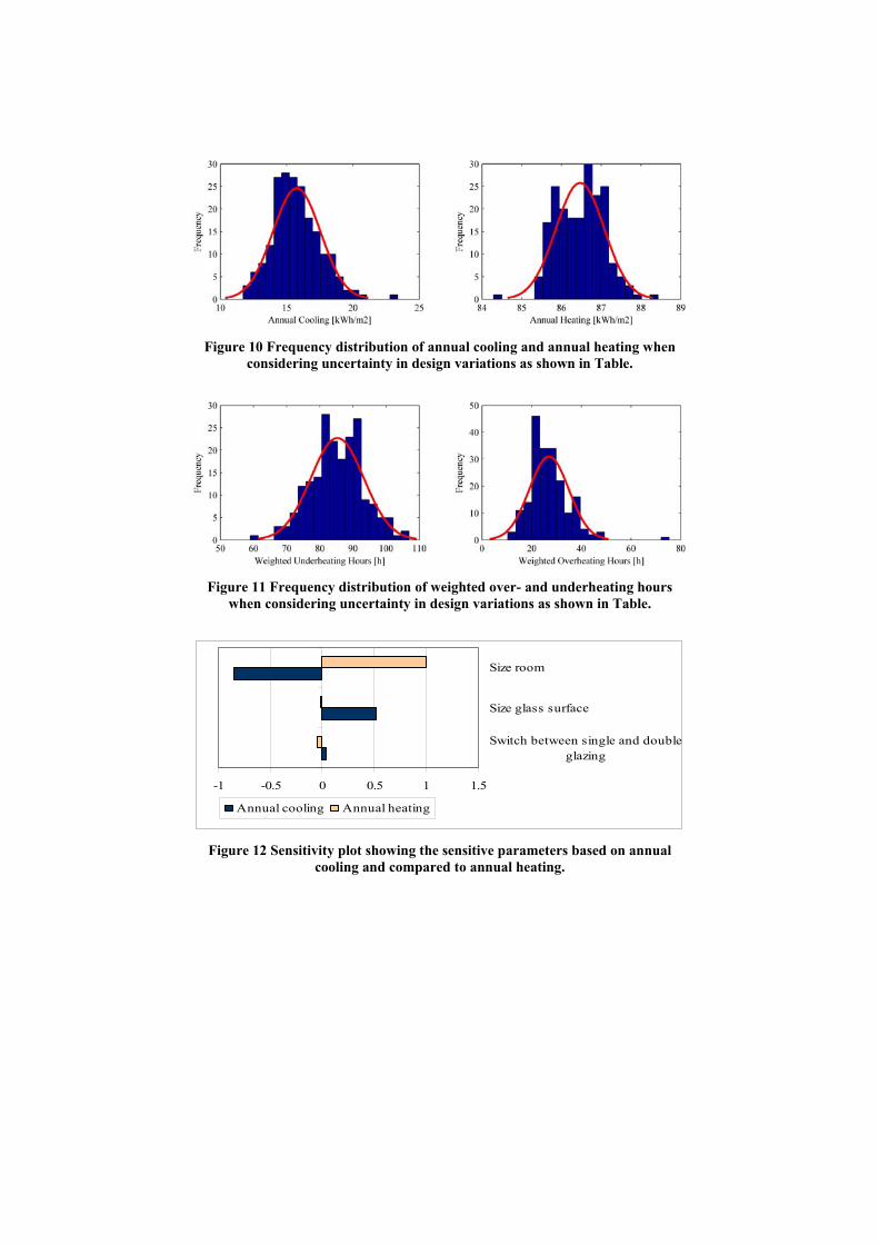
Figure 10 Frequency distribution of annual cooling and annual heating when considering uncertainty in design variations as shown in Table.

Figure 11 Frequency distribution of weighted over- and underheating hours when considering uncertainty in design variations as shown in Table.

-1 -0.5 0 0.5 1 1.5

Switch between single and doubleglazing

Size glass surface

Size room

Annual cooling Annual heating

Figure 12 Sensitivity plot showing the sensitive parameters based on annual cooling and compared to annual heating.

-1.5 -1 -0.5 0 0.5 1 1.5

Switch between single and doubleglazing

Size glass surface

Size room

Weighted underheating hours Weighted overheating hours

Figure 13 Sensitivity plot showing the sensitive parameters based on weighted underheating hours and compared to weighted overheating hours.