6 - 1

6. SPECIFIC APPLICATIONS

6.1 METHODS OF EXAMINATION

6.1.1 Cast work pieces

The defects in materials which occur during casting are piping (shrinkage), cavities or porosities, segregation, coarse grain structure, non-metallic inclusions and cracks.

Piping takes place during the solidification of an ingot. The outer layers are the first to solidify. During this time the liquid metal collects at the top of the ingot where after solidification is complete, a funnel-shaped cavity may appear due to the shrinkage. The shrinkage cavity will be either open or closed and, under certain circumstances, secondary cavities may be found.

The material of an ingot may not be homogeneous. Any variation in composition which arises during solidification is called segregation.

One type of segregation is gravitational, being caused by the separation in the upper part of the ingot of impurities having a lower temperature of solidification and a different density from the surrounding metal. This type of segregation consists primarily of sulphur or phosphorus.

A coarse grained structure may result when the pouring temperature is high and cooling takes place slowly. This sometimes makes it impossible to use ultrasonics because of the high attenuation in the material.

Gases dissolved in steel separate out when solidification occurs since their solubility in liquid metal decreases rapidly at this stage. If the gas content is high, gas cavities are often trapped under the surface or in the interior of the ingot.

Non-metallic inclusions, such as slag or refractories from the steel making process, find their way into the metal during melting or casting and are quite frequently the ultimate cause of fatigue cracks.

Longitudinal or transverse cracks may appear during solidification, depending on the method of construction of the mould, its temperature, the composition of the steel and the temperature of the melt.

In castings flaw detection almost exclusively concerns manufacturing defects such as shrinkage cavities, blow holes, inclusions (usually sand or slag) and cracks (caused by internal stresses during cooling while metal is already solidified).

Pure segregations are very rarely detected and then only by indirect means. Castings are seldom checked for fatigue cracks but, if required, the testing technique is similar to that used for forgings.

Basically, the demand made for the absence of flaws in the testing of castings cannot be as high as for worked components because the small shrinkage cavities and pores which are always present, produce some "grass" and small individual echoes even at low frequencies.

Both shear and compression wave techniques are widely used for the examination of castings. Because the grain structure has an appreciable effect on the attenuation of

6 - 2

ultrasonic waves, the test frequencies used in the examination of castings tend to be lower as compared to the frequencies used for the testing of other products. Frequencies of 1.25 MHz to 2.5 MHz are common and occasionally it is necessary to drop to 0.5 MHz in order to penetrate to the far boundary. The most commonly used probes are compression wave (single and twin crystal) and shear wave probes of 45°, 60° and 70°. The ultrasonic flaw detector used for the inspection of castings should therefore cover the frequency range 0.5 MHz to 6 MHz and when used with the probes selected for the job should have good resolution and penetration characteristics.

In the following some common defects in castings along with the techniques commonly used for their detection are discussed.

6.1.1.1 Shrinkage defects

Shrinkage defects are cavities formed during solidification i.e. during liquid to solid contraction. These defects are normally associated with gas, and a high gas content will magnify their extent.

Typical locations at which shrinkage cavities are most likely to occur are shown in Figure 6.1. Where there is a localized change of section thickness, a hot spot will occur which cannot be adequately fed. This will lead to shrinkage cavitation and should, therefore, be avoided if at all possible. Acute angle junctions (V, X or Y) are least satisfactory and T or L junctions are less of a problem.

Figure 6.1 : Typical locations for shrinkage cavities.

Shrinkage defects in steel castings can be considered as falling into three types, namely: Macro-shrinkage, Filamentary shrinkage, and Micro-shrinkage.

(a) Macro-shrinkage

Macro-shrinkage is a large cavity formed during solidification. The most common type of this defect is piping which occurs due to an inadequate supply of feed metal. In good design, piping is restricted to the feeder head.

The technique used to detect this defect depends on the casting section thickness. For sections greater than 75 mm thick, a single crystal compression wave probe can be used, whilst for thickness below 75 mm it is advisable to use a twin crystal probe.

The presence of a defect is shown by a complete loss of back wall echo together with the appearance of a new defect echo. An angle probe should be used to confirm the information gained from the compression wave probe (Figure 6.2).

6 - 3

Figure 6.2 : Typical probe positions for testing of casting for macro-shrinkage.

(b) Filamentary shrinkage

This is a coarse form of shrinkage, but of smaller physical dimensions than a macro-shrinkage cavity. The cavities may often be extensive, branching and interconnected.

Theoretically filamentary shrinkage should occur along the centre line of the section, but this is not always the case and on some occasions it extends to the casting surface. This extension to the casting surface may be assisted by the presence of pinholes or wormholes. Filamentary shrinkage can best be detected with a combined double probe if the section is less than 75 mm thick. Defect echoes tend to be more ragged in outline than for macro-shrinkage. The initial scan should be carried out with a large diameter (20-25 mm) probe and the final assessment with a smaller (10-15 mm) diameter probe (Figure 6.3).

Figure 6.3 : Double probe scanning of cast iron for filamentary shrinkage.

(c) Micro-shrinkage

This is a very fine form of filamentary shrinkage due to shrinkage or gas evolution during solidification. The cavities occur either at the grain boundaries (inter-crystalline shrinkage), or between the dendrite arms (interdendritic shrinkage).

Using a compression wave probe technique, the indications on the CRT screen from micro-shrinkage tend to be grass-like, that is, a group of relatively small poorly resolved echoes extending over some portion of the time base (Figure 6.4). The existence of a backwall echo in the presence of a defect echo will be to some extent dependent on the frequency chosen. For instance there may be no back wall echo when using a 4-5 MHz probe due to scattering of the beam. This might suggest a large angular type of defect. However, a change to a 1-2 MHz probe may well encourage transmission through the defective region to add a back wall echo to the defect echoes and disproving the large cavity impression.

6 - 4

Figure 6.4 : Probe positions and typical CRT appearance for micro-shrinkage.

6.1.1.2 Defects associated with hindered contraction during cooling

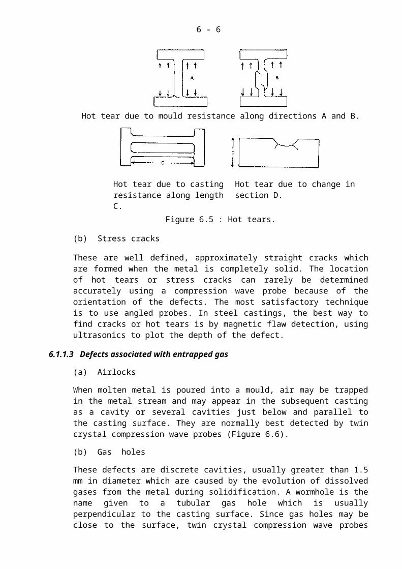
(a) Hot tears

These are cracks which are discontinuous and generally of a ragged form. They are caused by stresses which develop near the solidification temperature when the contraction of the cooling metal is restrained by a mould or core, or by an already solid thinner section. In Figure 6.5 some of the causes and locations of this type of cracking are shown.

Hot tear due to mould resistance along directions A and B.

Hot tear due to casting resistance along length C.

Hot tear due to change in section D.

Figure 6.5 : Hot tears.

(b) Stress cracks

These are well defined, approximately straight cracks which are formed when the metal is completely solid. The location of hot tears or stress cracks can rarely be determined accurately using a compression wave probe because of the orientation of the defects. The most satisfactory technique is to use angled probes. In steel castings, the best way to find cracks or hot tears is by magnetic flaw detection, using ultrasonics to plot the depth of the defect.

6 - 5

6.1.1.3 Defects associated with entrapped gas

(a) Airlocks

When molten metal is poured into a mould, air may be trapped in the metal stream and may appear in the subsequent casting as a cavity or several cavities just below and parallel to the casting surface. They are normally best detected by twin crystal compression wave probes (Figure 6.6).

(b) Gas holes

These defects are discrete cavities, usually greater than 1.5 mm in diameter which are caused by the evolution of dissolved gases from the metal during solidification. A wormhole is the name given to a tubular gas hole which is usually perpendicular to the casting surface. Since gas holes may be close to the surface, twin crystal compression wave probes are the most suitable probes to detect them (Figure 6.7).

Figure 6.6 : Typical probe positions and resulting CRT screen appearance for testing of air locks

Figure 6.7 : Typical probe positions and CRT screen appearance for detection of gas holes.

6.1.2 Welded work pieces

In the welding process, two pieces of metal are joined together. Molten filler metal from the welding rod blends with the molten parent metal at the prepared fusion faces, and fuses the

6 - 6

two pieces together as the weld cools and solidifies. Some of the defects occur because the fusion faces do not melt properly or blend with the filler metal (lack of penetration and lack of fusion defects). Some defects occur because the scale or slag which forms at the top of each pass of the welding, is not chipped away completely before the next pass is made (slag inclusions). Some defects occur because the welding electrode dips into the molten weld and bits of copper or tungsten drop into the weld (dense metal inclusions). Some defects occur in much the same way as casting defects (porosity, piping, wormholes, shrinkage, undercut, etc.). Some defects occur because of the thermal stresses, set up by having part of the component at molten temperature, and the rest of the parent material at much lower temperatures (cracks, tears, etc.).

Many of the defects which can occur in welds do not significantly alter the strength of the weld; others do in varying degrees. However, planar defects (cracks, lack of penetration / fusion) particularly those breaking the surface of the welded joint, give rise to the most severe reductions of weld strength.

6.1.2.1 Types of weld joints

Most welds fall into one of the following categories:

(i) Butt welds (ii) T-welds (iii) Nozzle welds

A butt weld is achieved when two plates or pipes of usually equal thicknesses are joined together using any of the weld preparations given in Figure 6.8.

Figure 6.8 : Various weld configurations for butt welds.

Figure 6.9 a illustrates the weld preparation for a typical single vee weld and the terms used to describe various parts of the prepared weld area. The same weld after welding is shown in Figure 6.9 b showing the original preparation and the number of passes made to complete the weld.

A T-weld is achieved when two plates are joined at right angle to each other. A T-weld may be fully penetrated (Figure 6.10 a) or only partially penetrated (Figure 6.10 b) by design.

6 - 7

Figure 6.9 a : Terms used to describe various parts of weld area.

Figure 6.9 b : Original preparation of weld and number of passes made to complete the weld.

Figure 6.10 : (a) Fully penetrated weld, (b) Partial penetration weld.

Nozzle welds are those in which one pipe is joined to another as a branch, either at right angle or some other angle. As with T-joints, the weld may be fully or only partially penetrated. The branch may get into the main pipe to let liquids and gases in or out, for instance, or the branch may simply be mounted on to an unperforated pipe, as in the case of a bracing strut in a tubular structure. The two types are shown in Figure 6.11 (a) and (b) in which the shaded portion shows the pipe wall.

(a) (b)

Figure 6.11 : (a) Branch pipe (b) Bracing strut.

6 - 8

Some typical weld preparations for nozzle welds are shown in Figure 6.12. In the diagrams the wall of the main pipe or vessel (called "shell"), and the wall of the branch, stub, or nozzle (called "branch") have been identified.

Figure 6.12 a : Fully penetrated "set on" weld. Figure 6.12 b : Partially penetrated "set in" weld.

Figure 6.12 c : Fully penetrated Figure 6.12 d : Partially penetrated "set through" weld. "set through" weld.

6.1.2.2 General procedure for ultrasonic testing of welds

The procedure for the ultrasonic testing of welds outlined below, if adhered to, will result in a speedy and efficient ultrasonic inspection of welds.

(a) Collection of information prior to the testing of weld

The information which has to be collected prior to testing a weld includes the following:

(i) Parent metal specifications.

(ii) Weld joint preparation.

(iii) Welding processes.

(iv) Parent metal thickness adjacent to the weld.

(v) Any special difficulty experienced by the welder during welding.

(vi) Location of any repair welds.

(vii) Acceptance standards.

(b) Establishment of exact location and size of the weld

To establish the exact location of the centre line of the weld, ideally, the parent metal should be marked on either side of the weld before the commencement of welding. In some cases where the weld reinforcement has been ground flush with the parent material, it may be necessary to etch the weld region to establish the weld width.

6 - 9

The centre line of the weld should be marked accurately on the scanning surface of the weld. For a single vee weld whose reinforcement has been ground flush with the parent metal, the centre line of the weld can be determined by marking the centre point of a normal probe at two or three locations on the weld (Figure 6.13 a) at which a maximum echo is obtained from the weld bead. The line joining these points is then the centre line of the weld. For single vee welds whose weld reinforcement has not been removed an angle beam probe can be used for this purpose, by placing the probe first on one side of the weld (Figure 6.13 b) and marking the probe index on the specimen where the echo from the weld bead is a maximum. On the same side of the weld two or three such points are obtained. Then the probe is placed on the other side of the weld and the probe index is again marked at different locations when a maximum echo from the weld bead is obtained. The centre points of lines joining these marks are then determined. When these points are joined the centre line of the weld is obtained.

(a) (b)

Figure 6.13 : Locating the centre line of the weld.

(c) Visual inspection

A visual check should be carried out prior to the commencement of testing to make sure that the surface is free from weld spatter and smooth enough for scanning. Some defects, e.g. undercut, etc., may show at the surface and be noticed during the visual examination. If these defects are in excess of the acceptance standard, then they should be remedied before carrying out the ultrasonic inspection.

Other faults, which should be looked for during visual inspection, are misalignment and mismatch (Figure 6.14). These faults may not always adversely affect weld acceptability, but they might interfere with subsequent ultrasonic inspection.

A clue to misalignment is often the widening of the weld cap because the welder tries to disguise this fault by blending the cap with the parent metal on either side.

Figure 6.14 : Misalignment and mismatch.

6 - 10

(d) Parent metal examination

The parent metal should be examined with a normal beam probe to detect any defects such as laminations, etc., which might interfere with the subsequent angle beam probe examination of the weld, and also to assess the thickness of the parent metal.

The examination should be over a band which is greater than the full skip distance for the shallowest angle beam probe (usually 70° probe) to be used, Figure 6.15 illustrates what would happen if a large lamination were present in the parent metal. The presence of a lamination causes the beam to reflect up to the cap giving a signal which might be mistaken for a normal root bead, and at the same time, misses the lack of penetration defect.

Figure 6.15 : Effect of a large lamination on the ultrasonic examination.

For parent metal examination either a single crystal or a twin crystal probe with a frequency that lies between 2 to 6 MHz can be used. The highest frequency in this range is preferred. The setting of sensitivity for this examination should be in accordance with the relevant specification or code of practice.

(e) Critical root examination

The next step is to make a careful inspection of the weld root area. This is because it is the root area in which defects are most likely to occur and where their presence is most detrimental. It is also the region in which reflections occur from the weld bead in a good weld and root defect signals will appear very close to the standard bead signal, i.e. it is the region in which the inspector is most likely to be confused. Technical details about the root examination are given in Sections 6.1.2.3 and 6.1.2.6.1 for single vee and double vee welds respectively.

(f) Weld body examination

After an examination of the weld root, the body of the weld is then examined for defects using suitable angle beam probes. Technical details about the weld body examination are described for each type of weld joint in the subsequent sections.

6 - 11

(g) Examination for transverse cracks

After having examined both the weld root and the weld body the next step is to detect transverse cracks breaking either top or bottom surfaces. Magnetic particle inspection is obviously a quick and effective method for detecting top surface cracks and therefore often ultrasonic inspection is done only to detect cracks breaking the bottom surface. If the weld cap has not been dressed, as in Figure 6.16, this scan is done parallel to the weld centre line alongside the weld cap with the probe inclined towards the centre. Since a crack tends to have a ragged edge, it is likely that some energy will be reflected back to the transmitter. A safer technique is to use a pair of probes, one transmitting and the other receiving. This is also shown in Figure 6.16. If the weld is dressed, a scan along the weld centre line and several scans parallel to and on either side of the weld centre line, from each direction, are done to give a full coverage of the weld.

Figure 6.16 : Weld scanning for transverse cracks.

(h) Determination of the location, size and nature of the defect

If any defect is found as a result of these examinations the next step is to explore the defect as thoroughly as possible to determine:

i) Its exact location in the weld.

ii) Its size parallel with the weld axis (i.e. length of the defect).

iii) Its size through the weld thickness.

(iv) Its nature (slag, porosity, crack, etc.).

(i) Test report

In order that results of ultrasonic examination may be fully assessed, it is necessary that the inspector's findings are systematically recorded. The report should contain details of the work under inspection, the equipment used and the calibration and scanning procedures. Besides the probe angle, the probe positions and flaw ranges should be recorded in case the results of the report need to be repeated.

6.1.2.3 Examination of root in single vee butt welds without backing strip in plates and pipes

6.1.2.3.1 Scanning procedure

The scanning procedure for the examination of the root consists of the following steps:

6 - 12

(a) Selection of probe angle.

(b) Calibration of time base on I.I.W V1 or V2 block for a suitable range. For parent metal thicknesses up to about 30 mm, a time base range of 100 mm is suitable.

(c) Determination of the correct probe angle using I.I.W V1 or V2 block.

(d) Marking the probe index on the probe using I.I.W V1 or V2 block.

(e) Calculation of 1/2 skip distance and 1/2 skip beam path length (1/2 skip BPL) for the selected probe.

(f) Marking of the scan lines at 1/2 skip distance from the weld centre line on both sides of weld (Figure 6.17 a).

(g) Setting the gain sensitivity for scanning and evaluation.

(h) A scan is made by moving the probe slowly from one end of the specimen to the other, so that the probe index always coincides with the scan line. To this end a guide is placed behind the probe in such a way that when the heel of the probe is butted to the guide, the probe index is on the scanning line (Figure 6.17 b). Flexible magnetic strips are very useful for this purpose. Areas with echoes from defects are marked on the specimen for subsequent examination to establish the nature and size of the defects.

Figure 6.17 : Scan procedure for root of single vee butt weld.

(i) With the probe index on the scanning line, a lack of penetration echo will occur at the half skip beam path range. If the weld is a good one, a root bead echo will occur at a small distance (depending on how big the weld bead is) away from the anticipated spot for a lack of penetration echo (Figure 6.18 a). If there is some root shrinkage or undercut, the echo from these defects will occur at a slightly shorter range than the critical range (Figure 6.18 b).

(a) (b)

Figure 6.18 : Root scanning; (a) for a good weld, (b) for root shrinkage.

6 - 13

(j) In addition, to determine whether an echo occurring during the root scan is due to lack of penetration, root undercut, root shrinkage, or root bead, the following points should also be taken into consideration.

(i) Since lack of penetration is a good corner reflector, the echo from it is quite big compared to an echo from root undercut or root shrinkage.

(ii) With a lack of penetration echo there will be no weld bead echo, whereas with root undercut, there almost always is.

(iii) The echoes from root undercut and root shrinkage maximize when the probe is moved backwards from the scanning line.

(iv) If the weld bead echo varies a lot in amplitude and position, then there is a great probability of defects in the root area.

(k) After having carefully examined the root, probing from one side of the weld centre line, a second scan is similarly done from the other side of the weld centre line to confirm the findings of the first scan. In addition, the second scan will also help in interpreting two other types of defects in the root area. The first one of these is shown in Figure 6.19. It is a small slag inclusion or gas just above the root.

Figure 6.19 : Root scanning for defects just above the root.

This defect might appear just short of the half skip beam path length when doing scan 1, leading to the guess that it might be root undercut or root shrinkage. If this were so scan 2 should put it just further than the critical range. But in fact the inclusion will show about the same place, i.e. just short again. Furthermore, from undercut the echo is expected to maximize when the probe is moved backwards in scan 1, but in the same scan the echo from the inclusion will maximize when the probe is moved forward. The echo from the inclusion will also maximize when the probe is moved forward in scan 2.

The second defect mentioned above is shown in Figure 6.20. This shows a crack starting from the edge of the root bead. From side 1 a large echo will appear just where the echo from undercut is expected and there will be no accompanying bead echo. From side 2, however, it is possible to get a bead echo as well as the defect echo.

Figure 6.20 : Scanning for a defect starting from the edge of the root bead.

6 - 14

6.1.2.3.2 Selection of the angle probe

Angle probe selection is a matter of compromise to obtain the maximum information from any examination, in the minimum time. Use as high a frequency probe as is practicable. In selecting the probe for the particular work in hand, take into account the following factors:

(a) Surface condition: A lower frequency is better on a rough surface from the point of view of coupling efficiency.

(b) Curved surface: small probes do not rock to the same extent as large ones.

(c) Type of material: The transmission of sound waves varies with basic material types, and with the condition of the material. In weld metal, which is often coarsely crystalline, the sound can be greatly impeded. This is especially true for austenitic stainless steel, where large crystals reflect some of the sound back to the receiver, often to the extent that ultrasonic testing is impractical.

(d) Internal metallurgical structure: The grain size in the parent material can also affect the transmission of sound. When the grain size, or the size of precipitates or inclusions begins to get greater than 10% of the wavelength it can refract or reflect sound, leading to attenuation or noise.

(e) Penetration: In a given material, low frequency waves will penetrate further, than high frequency waves.

(f) Resolution: High frequency probes have superior resolution characteristics, so that small flaws can be found more readily, than with low frequency probes.

(g) Accuracy: In general, high frequency probes provide greater accuracy in determining the size of the flaws.

(h) Scanning speed: Where large flaws are to be covered as in initial detection of flaws; large probes of low frequency, provide rapid scanning.

(i) Probe angle: The angle is selected to insure that an echo will be obtained from all flaws. Pay special attention to those that may be so oriented that a significant echo signal is not obtained, unless the probe angle is favourable for normal reflection. These are often the most significant flaws, e.g. lack of fusion on side walls and at the root, and cracks. The probe angles most generally suited to different thicknesses, are as given in Table 6.1 below, unless special conditions apply:

TABLE 6.1 : SUITABLE PROBE ANGLES FOR DIFFERENT THICKNESS RANGES

Probe angle Thickness range

80 5 to 15 mm (0.2 to 0.6 in.)

70 15 to 35 mm (0.6 to 1.4 in.)

60 35 to 100 mm (1.4 to 4 in.)

45 50 to 200 mm (2 to 8 in.)

35 100 to 200 mm (4 to 8 in.)

In specific cases a departure from this table might be advisable. In choosing a beam angle, remember, that a beam incident on a reflecting surface at 30 will result in mode conversion, and in a loss of shear wave energy of up to 20 dB (90%). Further, a fraction of surface waves is generated by 80 probes and must be allowed for.

6 - 15

(j) Range selection: Make the beam path, in relation to frequency, sufficiently short, to avoid excessive attenuation. Subject to considerations of probe angle, nature of defects and beam spread, the representative ranges may be up to 200 mm (8 in) for frequencies of 2 to 6 MHz and up to 400 mm (16 in) for frequencies of 1 to 1.5 MHz.

6.1.2.4 Examination of weld body of a single vee butt weld without backing strip

After the root examination is complete, the weld body examination is then done using the following procedure:

(a) Selection of an appropriate probe angle.

(b) Calculation of the 1/2 skip and fullskip distances and 1/2 skip and full skip BPLs for the selected probe angle.

(c) Marking the parent metal on both sides of the weld with lines parallel to the weld centre line and at distances of 1/2 skip and full skip +1/2 cap width.

(d) Calibration of the time base for an appropriate range.

(e) Setting the sensitivity of the probe/flaw detector system for the maximum testing range which in this case is the full skip BPL.

(f) Scanning the specimen in a zigzag pattern between the marked scan limits (Figure 6.21). Each forward scan should be at right angle to the weld centre line, and the pitch of the zigzag should be a half probe width to ensure full coverage.

Figure 6.21 : Zigzag scanning of weld body.

(g) Mark the areas, in which defect echoes occur, for subsequent location, establishment of nature and sizing of the defects. The probe movement such as in Figure 6.22 may be used to help in establishing the nature and size of defects.

Figure 6.22 : Probe movements for establishing the nature and size of defects.

6 - 16

6.1.2.4.1 Selection of probe angle

The initial choice of probe angle for the weld body scan depends upon the weld preparation angle. The angle should be chosen to meet any lack of sidewall fusion at right angle for maximum response. The exact angle to meet this fusion face at right angle can be calculated from:

Probe angle = 90 - /2 ---------------------------------------- (6.1)

where, = weld preparation angle

Example (i):

Weld preparation angle = 60

Required probe angle = 90 - 60/2 = 90 - 30 = 60

Example (ii):

Weld preparation angle = 45

Required probe angle = 90 - 45/2 = 90 - 22.5 = 67.5

In the first case, clearly we would use 60 probe, but in the case of the 45 weld preparation angle, it is not likely that we will have a 67.5 probe, so we would choose the nearest, i.e. a 70 probe.

TABLE 6.2 : RELATIVE CHANGE IN PROBE ANGLES FOR DIFFERENT MATERIALS

Material Beam angle (Degrees)

Steel 35 45 60 70 80

Aluminium 33 42.4 55.5 63.4 69.6

Copper 23.6 29.7 37.3 41 43.4

Grey cast iron (mean value for lamellar cast iron)

23 28 35 39 41

6.1.2.4.2 Calculation of various distances for angle beam probes

Half skip and full skip distances and beam path lengths

Figure 6.23 defines the half-skip distance (HSD), full-skipdistance (FSD), half-skip-beam-length (HSBPL) and full-skip-beam-length (FSBPL) for an angle beam probe of refraction angle.

Distance AB = Half-Skip Distance (HSD)

Distance AC = Full-Skip Distance (FSD)

Distance AD = Half-Skip-Beam-Path-Length (HSBPL)

Distance AD + DC = Full-Skip-Beam-Path-Length (FSBPL)

6 - 17

Figure 6.23 : Various skip distances and beam path lengths for an angle beam probe.

The relations used to calculate HSD, FSD, HSBPL and FSBPL for a specimen of thickness t, are given below:

HSD = t x tan ---------------------------------------------- (6.2)

FSD = 2t x tan ---------------------------------------------- (6.3)

HSBPL = t/cos ---------------------------------------------- (6.4)

FSBPL = 2t/cos ---------------------------------------------- (6.5)

If the actual probe angle is exactly equal to the nominal probe angle then these distances can be calculated by the following formula:

Distance required = F x t ------------------------------------- (6.6)

where F is the appropriate factor from Table 6.3.

TABLE 6.3 : F FACTOR FOR VARIOUS DISTANCES WITH ANGLE BEAM PROBES

Probe angle

F factor

35 45 60 70 80

HSD factor 0.7 1.0 1.73 2.75 5.67

FSD factor 1.4 2.0 3.46 5.49 11.34

HSBPL factor 1.22 1.41 2.0 2.92 5.76

FSBPL factor 2.44 2.83 4.0 5.85 11.52

6.1.2.5 Inspection of single vee butt welds with backing strips or inserts

The inspection procedure for such welds only differs from that for single vee welds without backing strips in the detail of the critical root examination. In the root examination of this type of weld, the prime object is to confirm that fusion has taken place between the parent metal, root preparation and the backing strip or insert.

6.1.2.5.1 Welds with EB inserts

When properly fused, this weld configuration is like a perfect single-vee weld with a constant root bead profile. Setting up for a root examination is exactly the same as for a single-vee butt weld without a backing strip. Scanning along the probe guide will give a root

6 - 18

bead echo which occurs at a particular place on the time base and which remains constant in amplitude (provided, of course, couplant and surface roughness are also uniform). A drop in the amplitude of this echo is a clue that fusion may not be complete. The presence of an echo at exactly half skip beam path length is positive evidence of non-fusion. Since the insert gives a very strong echo as a rule and that echo is only 2-3 mm beyond the half skip beam path length position, a short length of non-fusion is only shown as half skip beam echo sliding up the front of the insert echo (i.e. poorly resolved), as shown in Figure 6.25. The angle of the probe should be chosen to meet any lack of side wall fusion at right angle for maximum response. The exact angle to meet the fusion face at right angle can be calculated from Equation 6.1 .

The range at which the testing is done, particularly using a 70 probe to suit the weld preparation angle, can be quite long and the sensitivity to defects other than lack of side wall fusion may be rather low. In such cases it is reasonable to use 45 or 60 probes to carry out supplementary scans. If the weld cap has been dressed, this problem can be overcome by scanning across the weld centre line from half skip to the far edge of the original cap instead of changing the probe. Care should be taken to ensure that any residual undulation left when the cap is dressed, is not severe enough to lift the probe index clear of the surface (Figure 6.24).

Figure 6.24 : Scan for root bead with EB inserts.

Figure 6.25 : CRT indication for lack of fusion at root.

Lack of fusion at the top of the insert (Figure 6.26) can best be detected by a longitudinal wave probe. For this reason it is desirable for the weld cap to be dressed to allow the normal beam probe scan. If this cannot, or has not been done, this defect can often be found as an echo originating from just above the root, when using an angle beam probe because of distortion or entrapped slag.

Figure 6.26 : Normal beam probe scan for lack of fusion at the top of EB inserts.

6 - 19

6.1.2.5.2 Welds with backing strips

When properly fused the weld cross section looks like the one shown in Figure 6.27a. An angle beam probe scan allows energy to pass through the root into the backing strip. Reflection from within the strip will be shown as pattern of echoes beyond the half skip beam path length (Figure 6.27 b). A decrease in amplitude or total loss of this pattern indicates non-fusion of the backing strip. Again, it is desirable to have the weld cap dressed so that a normal beam probe can be used to check the root fusion. With a normal beam probe over the weld centre, an echo will be received from the back wall, and from the backing strip. Loss of the backing strip echo indicates lack of fusion (Figure 6.28 c).

(a)

(b) (c)

Figure 6.27 : (a) Cross section of welds with backing strip, (b) CRT indication of root scan with angle beam probe, (c) with normal beam probe.

6.1.2.6 Inspection of double vee welds

The routine for double-vee welds is basically the same as that for single-vee welds. There are some differences in detail in the critical root examination and the weld body scan, because of the difference in weld configuration. These differences are discussed in the following paragraphs.

6.1.2.6.1 Critical root scan for double vee welds

The typical weld preparation for a double vee weld is shown in Figure 6.28 which also shows the theoretical lack of penetration defect in this type of weld. It can be seen that, in theory at least, this defect which is planar, vertical and in the middle of the weld volume, ought not to reflect sound back to the probe. In practice, however, there is often enough slag or distortion at the top or bottom of the defect to give a reflection. It is usual, therefore, to use a 70 probe, positioned at 1/4 skip distance from the weld centre line, to carry out the critical root scan. The anticipated time base range for an echo from lack of penetration cannot be predicted as precisely as for single-vee welds, but, of course, echoes from root bead or undercut do not occur in this type of weld configuration.

Another method that can be used for the examination of the root in double vee welds, and for that matter for the detection of any vertical reflecting surface within the volume of a

6 - 20

material, is the tandem technique shown in Figure 6.28. Here = probe angle, S = separation between probe indices, d = depth of aiming point, and t = specimen thickness. For double vee welds, the beam is aimed at the centre of the weld (i.e. d = 1/2 t), and the probe separation S is equal to half skip distance for that probe angle. For other applications the probe separation for any depth can be calculated from the following formula.

S = 2 (t - d) tan ------------------------------------------------------------------ (6.7)

Figure 6.28 : Tandem technique for double-vee welds scan.

6.1.2.6.2 Weld body examination for double-vee welds

The weld body examination of double-vee welds is much the same as for single vee welds, but this time the scan starts at 1/4 skip distance from the weld centre and goes back to full skip plus half weld cap width (Figure 6.29). In this type of weld configuration there are four fusion faces to be examined, and the reflections from the bottom weld cap, which occur between half skip beam path length and 3 to 4 mm beyond half skip beam path length, will prevent confirmation of the condition of the lower fusion face on the opposite half of the weld.

Figure 6.29 : Marking scan area for double-vee welds.

6.1.2.7 Examination of T-welds

In the case of a T-weld configuration, for complete inspection of the weld, access to several surfaces is required. In practice, access to more than one surface may not be available and thus only limited inspection of the weld can be carried out.

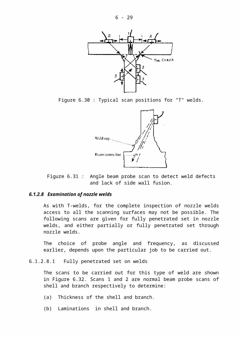
The inspection procedure for both partially penetrated and fully penetrated (for types of T-weld configuration see Figure 6.12 a & b ) T-welds is much the same, but for partially penetrated welds monitoring of the non-fused portion of the weld is needed to ensure that it is not longer than the design permits. For an ideal case where all surfaces are readily accessible, the scans to be made for the complete inspection of a T-weld are illustrated in Figure 6.30. Scan 1 is done with a normal beam probe to detect laminations, lack of fusion and lamellar tearing. Scan 2 is done with an angle beam probe to detect weld body defects and toe cracks and scan 3 is an angle beam probe scan to detect weld defects and lack of side wall fusion.

6 - 21

As with the previously discussed weld configurations, probe angles and frequencies are to be chosen to suit the particular job. For scan 3 it is useful to choose a probe angle which will produce a beam centre line parallel to the weld cap (Figure 6.31) to reduce the tendency for confusing cap echoes.

Figure 6.30 : Typical scan positions for "T" welds.

Figure 6.31 : Angle beam probe scan to detect weld defects and lack of side wall fusion.

6.1.2.8 Examination of nozzle welds

As with T-welds, for the complete inspection of nozzle welds access to all the scanning surfaces may not be possible. The following scans are given for fully penetrated set in nozzle welds, and either partially or fully penetrated set through nozzle welds.

The choice of probe angle and frequency, as discussed earlier, depends upon the particular job to be carried out.

6.1.2.8.1 Fully penetrated set on welds

The scans to be carried out for this type of weld are shown in Figure 6.32. Scans 1 and 2 are normal beam probe scans of shell and branch respectively to determine:

(a) Thickness of the shell and branch.

(b) Laminations in shell and branch.

(c) Lack of fusion of shell wall.

(d) Weld body defects.

6 - 22

Figure 6.32 : Scans for fully penetrated "set on" welds.

Scan 3 is a critical root scan. Scan 4 is the scan made by moving the probe between half skip and full skip limits. This scan is done to determine lack of side wall fusion and weld body defects.

6.1.2.8.2 Partially penetrated set in welds

The scans are similar to those shown in Figure 6.32. However, in this case it is necessary to check the actual penetration achieved and to make sure that the horizontal fusion face is fused (Figure 6.33 a & b). This can be achieved, with practice, by very carefully plotting

Figure 6.33 : (a) Intended condition, (b) Faulty condition.

the root echoes. It is usual to plot both the maximum reflecting point, and, as confirmation, the point at which the echo just disappears (i.e. beam centre and beam edge). From an accurate scale drawing, the intended point of maximum penetration can be determined, and the range of this point, using the beam centre and beam edge, can be measured. Probe positions corresponding to these reflecting points can also be measured and compared to those achieved during the scan.

If, in practice, both points occur at probe positions closer to the shell than the predetermined positions, then the penetration is somewhat deeper than intended. If they occur further from the shell than expected, a condition such as the one shown in Figure 6.33 b would be suspected.

6.1.2.9 Examination of brazed and bonded joints

(i) Brazed joints

If the wall thickness permits clear separation between back wall echoes, brazed joints can be examined using the standard procedure for lamination testing. However, since the brazed metal separating the two brazed walls will have a slightly different acoustic impedance from that of the brazed walls, a small interference echo will be present for a good braze. The technique is, therefore, to look for an increase in this interface echo amplitude (Figure 6.34 a, b, c).

6 - 23

Figure 6.34 (a,b,c) : Ultrasonic inspection of brazed joints.

If the two brazed wall thicknesses are too thin to permit clear back wall echoes, a multiple echo, as described for lamination testing, can be used.

(ii) Bonded joints

These may include metal to metal glued joints and metal to non-metal glued joints (e.g. rubber blocks bonded to steel plates). The technique used is a multiple echo technique. Each time the pulse reaches a bonded interface, a portion of the energy will be transmitted into the bonded layer and absorbed. Each time a pulse reaches an unbonded layer, all the energy will be reflected. The decay of the multiple echo pattern for a good bond would, therefore, be short because of the energy loss at each multiple echo into the bond (Figure 6.35). However, for an unbonded layer each multiple echo will be slightly bigger because there is no interface loss, and the decay pattern will be significantly longer (Figure 6.36).

Figure 6.35 : Echo pattern indicating good bonded joint.

6 - 24

Figure 6.36 : Echo pattern showing lack of bonding.

6.1.3 Components and systems

6.1.3.1 Ultrasonic testing in the automotive industry

Large production volume and integrated testing in the production line characterize testing in the automotive industry. Therefore a testing machine must have a high degree of automation and be able to test quickly. The following describes ultrasonic testing machines used in the automotive industry.

6.1.3.1.1 Testing of irregular shaped parts

Axle stubs, pivot bearings, brake callipers, etc. are parts which due to the material used (mostly nodular cast iron) and the method of production (casting), must be tested for flaws in critical areas (Figure 6.37 a & b).

(a) (b)

Figure 6.37 (a & b): Ultrasonic probe arrangements for automatic scanning of irregular shaped automobile parts.

6.1.3.1.2 Testing of rotational symmetrical parts

Valves, valve seating rings, cup tappets and gears can, due to their symmetrical shape, be rotated within the sound beam of a fixed probe in order to test a certain area. Figure 6.38 (a & b) shows an example of testing round welds (laser or electron beam welds) for inclusions on cup tappets and valve seating rings.

6 - 25

(a) (b)

Figure 6.38 (a & b) : Ultrasonic probe arrangements for automatic scanning of symmetrically shaped automobile parts.

6.1.3.2 Ultrasonic testing in the aerospace industry

Operational safety is of major importance in the aerospace industry. This is the reason why the demands are very high regarding the detection of material flaws and material inhomogeneities together with documentation. The only instruments and systems which fulfill these requirements are the ones with the highest possible resolution power, very good evaluation accuracy and reliable self monitoring functions.

6.1.3.2.1 Testing of turbine parts using the immersion technique

These parts are subject to very high stresses. The smallest flaws and inhomogeneities can, with a high revolution rate of the parts, extend and cause a dangerous state of unbalance thus leading to damage. With turbine disks testing must be made at an early processing stage to detect critical flaws in order to avoid further processing costs.

To test these unfinished turbine disks or other rotationally symmetrical parts the ultrasonic immersion testing machine is used. Laminar defects and according to the rate of occurrence and the distribution, inclusions as well as porosities are critical flaws in rotor blades. Testing of the rotor blades is made via the immersion technique using through transmission method, often using focusing probes. A print out or a C-scan can be made of the test results (Figure 6.39).

Figure 6.39 : Immersion testing of rotor blades.

6 - 26

6.1.3.3 Ultrasonic testing of rolled products

Rolled products are mostly long and must sometimes be tested in the production line. This nearly always means automatic ultrasonic testing at high transport speeds so that the production flow is not slowed down in any way. It is always better to detect flaws while the product is in the semi-finished state, in this way production of the defective part can be stopped thus saving costs.

6.1.3.3.1 Tube testing

For the testing of seamless tubes and welded tubes with the bead ground off there are two different types of testing which can be used depending on the diameter of the tube. Tubes with an outside diameter of up to 180 mm are transported in a straight line through the testing machine. Longitudinal and transverse flaw testing is carried out with probes housed in a water chamber which rotates around the tube. The allocation of further probes enable monitoring of the geometrical data such as wall thickness, outside and inside diameter, ovality and eccentricity. Large tubes with outside diameters of up to 600 mm are spirally transported via water filled tanks which contain the probes (partial immersion technique). With the large tube testing machine up to 40 probes test for longitudinal and transverse flaws as well as measuring the wall thicknesses simultaneously .

By distributing the probes optimally in a number of probe modules, testing of short untested tube ends can be achieved. If wall thicknesses are to be measured only over a number of tracks then in most cases the tube is transported through the measuring position without being rotated.

The same testing techniques as used for round bar testing (Section 6.1.3.3.3) are applicable to tube testing. The only difference, of course, is that there are no core defects. However, surface flaws can occur on the inner as well as outer surfaces of the tubes. In seamless and rolled pipes, the defects (Figure 6.40) which are of interest are similar to those occurring in rod materials, for example incipient cracks and spills in the internal and external surfaces. Laminations can also appear in the wall as a result of the manufacturing process.

Figure 6.40 : Types of defects and main direction of testing in pipes.

Since the smallest possible angle is 35, the ratio of wall thickness to tube diameter (d/D), at which a test for internal flaws is still possible, must not exceed 0.20. Should there be a need for testing tubes with thicker wall (i.e. d/D > 0.2) for cracks on their internal surface, the angle of incidence must be less than 35. This can be achieved by attaching an obliquely ground perspex shoe to a normal probe (Figure 6.41). Since both longitudinal and transverse

6 - 27

waves are produced simultaneously, many interfering echoes which are not defect echo indications appear on the screen. Fortunately, these can be distinguished from flaw echoes when the probe or the tube is rotated, since flaw echoes move across the CRT screen whereas the interfering echoes remain stationary.

Figure 6.41 : Testing method for detecting longitudinal surface defects on internal surfaces of thick wall tubes using normal probes.

6.1.3.3.2 Calculation of maximum penetration thickness for thick wall pipes

The normal range of transverse wave angle beam probes (45, 60and 70) when used on thick wall pipes may not penetrate to the bore of the pipe, but cut across to the outside surface again, as shown in Figure 6.42 and miss the defect.

Figure 6.42 : Diagram showing how the defects lying on the inner surface of a thick-wall pipe may be missed by an angle beam probe.

For a given probe angle, the maximum wall thickness of a pipe that allows the centre of the beam to reach the bore of the pipe can be calculated from the following formula:

t = d (1 - sin )/2 --------------------------------------------- (6.8)

where,

t = maximum wall thickness

d =outer diameter (OD) of the pipe

= probe angle

Equation 6.8 can be rewritten to determine the best angle for a given wall thickness as:

= sin-1 (1-2t/d) --------------------------------------------- (6.9)

For convenience Equation 6.6 can be simplified for standard angle probes as

t = d x F ----------------------------------------------------------------- (6.10)

6 - 28

where,

F is the probe factor given in Table 6.4.

TABLE 6.4 : VALUES OF PROBE FACTOR ‘F’ FOR VARIOUS ANGLES

Probe angle () 35 45 60 70 80

Probe factor (F) 0.213 0.146 0.067 0.030 0.0076

Table 6.5 gives values of maximum wall thickness for various pipe sizes and probe angles.

TABLE 6.5 : VALUES OF MAXIMUM WALL THICKNESS FOR VARIOUS PIPE SIZES AND PROBE ANGLES

Probe angle Maximum wall thickness

Pipe O.D 35 45 60

4" (100 mm) 21.3 mm 14.6 mm 6.7 mm

6" (150 mm) 31.95 mm 21.9 mm 10.05 mm

8" (200 mm) 42.6 mm 29.2 mm 13.4 mm

10" (250 mm) 53.25 mm 36.5 mm 16.75 mm

12" (300 mm) 63.9 mm 43.8 mm 20.1 mm

14" (350 mm) 74.55 mm 51.1 mm 23.45 mm

16" (400 mm) 85.2 mm 58.4 mm 26.8 mm

18" (450 mm) 95.85 mm 65.7 mm 30.15 mm

20" (500 mm) 106.5 mm 73.0 mm 33.5 mm

6.1.3.3.3 Rod testing

Rods have diameters up to approximately 50 mm and are either round, square or hexagonal in shape. These are often tested only in the core area. In this case it is sufficient to scan the core area with two probes, which are off-set by 90 or 60 around the circumference and move the rods linearly past the probes. With an additional TR probe, rods having diameters between 50 mm and approximately 100 mm are tested. Rods up to 50 mm are transported via two guiding stations through the water filled test chamber. Depending on the profile shape the two probes are off-set by 60, 90 or 120 (Figure 6.43).

If, with round rods, a greater material area is to be tested beyond the core area then the rotational testing machine should be used as long as the rod diameter does not exceed 180 mm.

For the simultaneous detection of internal and surface flaws on round material with diameters of up to 500 mm the rods are spirally fed over the probe holders, whereby water gap coupling is applied.

6 - 29

Figure 6.43 : Ultrasonic probe arrangements for automatic testing of rods and billets.

6.1.3.3.4 Plate testing

Flaws in plates such as laminar defects and inclusions can, if the plate is further processed, lead to new flaws. If, for example, defective plates are cut and then welded to other components then welding defects in the area of the cut edge of the plate can often be traced back to an inclusion. Also it is a fact that defects already in the basic material very often cause rejects at the sheet table when the plate is rolled to form sheets.

The standard procedure which is used to test for laminations in plates and pipes, which are to be welded or machined, is given below:

(i) Calibrate the time base to allow at least two back wall echoes to be displayed.

(ii) Place probe on the lamination free portion of test specimen and adjust the gain control so that the second back wall echo is at full screen height.

(iii) Scan the test specimen looking for lamination indications which will show up at half specimen thickness together with a reduction in back wall echo amplitude. In some cases a reduction in the amplitude of the second back wall echo may be noticed without a lamination echo being present. Care must be taken to ensure that this reduction in amplitude is not due to poor coupling or surface condition.

Lamination testing of plate or pipe less than 10 mm in wall thickness may be difficult using the standard procedure because multiple echoes are so close together that it becomes impossible to pick out lamination echoes between back wall echoes. In such cases a technique, called the multiple echo technique, using a single crystal probe can be used. The procedure is as follows:

(i) Place the probe on a lamination free portion of the test specimen or on the calibration block.

(ii) Adjust the time base and gain controls to obtain a considerable number of multiple echoes in a decay pattern over the first half of the time base (Figure 6.44 a).

6 - 30

(iii) Scan the test specimen. The presence of a lamination will be indicated by a collapse of the decay pattern such as the one shown in Figure 6.44 b. The collapse occurs because each of the many multiple echoes is closer to its neighbour in the presence of a lamination.

The above mentioned flaws can be ultrasonically detected by using straight beam probes. With the exception of random testing it is not advisable to carry out a plate test manually. Due to the simple geometry of the test object an automatic test in the production line is the best solution. However, the selection of the most suitable testing machine is determined by the plate thickness, the number of plates to be tested, the maximum test time and the conditions at the test location (is the testing machine to be integrated into the production line (on-line) or is the test to be made external to the production line (off-line)).

Figure 6.44 : Multiple echo decay pattern from plate; (a) Without lamination, (b) With lamination.

6.1.3.3.5 Rail testing

Defective rails can lead to very serious accidents and cause extensive damage. Many railways carry out routine checks on the tracks of railway lines. In addition to this, rails are tested with ultrasonics during production. Flaws in the rail head, web and foot can be detected during production, in some cases detection of the rail stamp in the web should be possible.

For this type of testing dual probes and angle beam probes are used. Their testing position is dependent on where typical flaws are likely to occur.

6.1.4 Austenitic materials

It is difficult to test cast stainless steel to high degree of reliability because of the coarse grain and highly variable microstructure of the material (Figure 6.45 a & b).

6 - 31

Cast stainless steel can have a well defined equiaxed grain structure, a well defined columnar grain structure or mixed grain structure (Figure 6.46 a & b). Because ultrasonic beam distortions are related to the material microstructure and the selected test procedure, the ability to interpret data depends on knowledge of the microstructure. Because the microstructure can be obtained by measuring the velocity of sound, this is an effective and reliable way to non-destructively assess the inspectability of a component, even under field conditions.

(a)

(b)

Figure 6.45 : Grain size and CRT screen display; (a) before normalizing, (b) after normalizing.

(a) (b)

Figure 6.46 : A coarse grain formation; (a) after an austenitic weld structure, (b) after heat treatment.

When cast stainless steel is composed of isotropic equiaxed grain the variation in velocity with propagation direction is small (less than 2 percent) . For an anisotropic material composed of columnar grains the variation in velocity may be large, as much as 100 percent for shear waves (Figure 6.47). The magnitude of the sound velocity may also be used as a measure of anisotropy. Relatively low longitudinal wave velocity indicates a columnar grain structure and high velocities indicate an equiaxed structure. Intermediate values indicate the presence of both microstructures.

6 - 32

Figure 6.47 : An anisotropic structure.

Ultrasonic angle beam shear waves travel easily from wrought base metal through low alloy carbon steel welds. In austenitic stainless and high nickel alloys welds, the shear beam may be reflected at the fusion line or deflected in the weld metal because of velocity and grain structure differences. Discontinuity indications from the reflective fusion line may appear to be from incomplete fusion. Reflective fusion line indications can cause the unnecessary repair of good welds. For this reason reflective interface indications are tested with a longitudinal wave beam of the same angle. The longitudinal wave angle beam may not reflect from the interface but does reflect from incomplete fusion permitting identification of the indication.

Improved austenitic weld tests have been reported at low frequencies (1.5 MHz) with short pulse lengths. Focusing or dual transducers improve the signal-to-noise ratio. A narrow sound beam can have favourable effects with regard to testing austenitic welds . The ratio can also be improved by using longitudinal wave angle beams that are not sensitive to grain structure.

6.1.5 Forged work pieces

Manufacturing defects occurring in such semi-finished products can either be internal defects or surface defects. Some internal defects originate from ingot defects in the core such as shrinkage cavities and inclusions which are elongated during rolling, forging or drawing. Others are rolling and drawing defects such as cracks in the core, radial incipient cracks on the rod surface or spills which penetrate to the surface at a small angle. Since most flaws in rods or billets extend in the longitudinal direction, this requires that the axis of the sound beam be in a cross sectional plane (Figure 6.48) either normal or oblique to the surface. Also used are surface waves in the circumferential direction.

Figure 6.48 : Types of defects in round stock and main directions of testing.

6.1.5.1 Billets.

These often have longitudinally directed flaws in the core zone (pipings, cracks and inclusions) or on the surface (cracks).

6 - 33

The core flaws are detected by using two normal probes connected in parallel, as shown in Figure 6.49 for square billets. In this test, a great part of the billet is not tested (Figure 6.50) owing to the beam position as well as the dead zones of the probes. Therefore, when testing square billets with sides shorter than 100 mm, SE (double crystal) probes are used. It goes without saying that SE probes with heavily inclined oscillators cannot be used since their maximum sensitivity is just below the surface. Normally the so-called 0° (zero degree) SE probes are used. Longitudinal surface flaws on square billets are practically impossible to detect with normal, SE or even angle probes.

Figure 6.49 : Testing billets with two probes connected in parallel.

Figure 6.50 : Incomplete coverage by normal probes used for testing of square billets.

The testing procedure with normal probes for core flaws mentioned earlier is also applicable for round billets but with more difficulty, especially when testing by hand, because of the curved surface which reduces contact area and probe sensitivity (Figure 6.51). The contact area can be increased by using a perspex shoe whose front curvature fits closely to the round billet (Figure 6.52).

Because divergence of the sonic beam, even with a probe with a shoe, gives rise to disturbing echoes between the first and second back-wall echoes, core flaws in round billets are usually checked with SE probes.

Figure 6.51 : Difficulty in testing round billets with normal probesdue to reduced contact area.

Figure 6.52 : Increase in contact area by using perspex shoe.

Longitudinal surface flaws in round billets can be detected with angle probes provided the

6 - 34

surface is not too rough. For a 45° or 60° angle probe which is suitably ground as shown in Figure 6.53, the broad beam, after a few reflections, fills a zone under the surface up to a depth of about one-fifth of the diameter. If a longitudinally oriented surface flaw is present (Figure 6.54), an echo will be visible on the CRT screen; otherwise no echo is visible. It is possible to miss a flaw that is at an acute angle to the surface (Figure 6.55). Therefore, in order to be able to detect all surface flaws, the angle probe must be turned round by 180° and also moved around the billet or the billet itself must be turned. The flaw echo then will move across the screen with alternating heights, having a peak height just before the transmission pulse.

Figure 6.53 : Depth of penetration of oblique transverse waves in round billets.

Figure 6.54 : Detection of longitudinal surface flaws in round billets using angle probes.

Figure 6.55 : Possibility of missing longitudinal surface flaws in round billets using angle probes.

With the billet rotating and the angle probe advancing longitudinally, a spiral scan can be performed, enabling all of the billet to be tested.

6 - 35

6.1.5.2 Rod materials

There is hardly any difference between testing round billets and bars for cracks, shrinkage or inclusions. To find defects in the core, it is sufficient to scan along at least two longitudinal tracks using a normal or an SE probe depending on the rod diameter. As in round billets, surface defects are detected with oblique transverse waves or with surface waves when the surface is sufficiently smooth.

The use of a twin angle probe allowing a flowing water coupling, enables bars to be tested with increased speed. A bar without a surface flaw will give a large echo on the CRT screen (Figure 6.56). This echo is caused by the sound beam, emitted by one oscillator, being received by the other and vice versa. Both sonic pulses have to cover the same distance corresponding to a circular measure of about 360°. Since the flaw detector is adjusted to half sound path, the common echo will appear on the screen at a distance corresponding to 180°. As the length of the sound path between the oscillators does not alter when shifting the twin angle probe or rotating the bar, provided the bar diameter is constant, the so-called control echo position on the CRT screen remains constant. Hence, any longitudinal surface flaw can easily be distinguished from this echo, since the flaw echo position on the screen is not constant. When the probe is moved in the direction of a surface flaw, the flaw echo arriving at the nearest oscillator and appearing between the transmission pulse and the control echo will move towards the transmission pulse (Figure 6.56). The echo arriving at the farther oscillator is visible at the right of the control echo and moves in the opposite direction. This echo is rather small and therefore is not usually employed for flaw detection. If the probe or rod is moved until the high flaw echo is exactly in the middle between transmission pulse and control echo, the flaw must be located exactly one fourth of the bar circumference from the probe position (Figure 6.57).

Figure 6.56 : Testing of round bar with twin angle probe.

Figure 6.57 : Location of surface flaw on rod using twin angle probe.

6 - 36

6.1.5.3 Use of immersion technique for billet or rod materials

Test speed can be maximized by the use of the immersion technique (Figure 6.58), especially for small rod diameters. In this technique, the test specimen is immersed in water and immersion probes are used. When a normal probe is used, it is possible to generate all types of waves (Figure 6.59) by moving the probe position or direction. If the beam is broad, several waves can sometimes be obtained simultaneously. If the surface is not sufficiently smooth, this may give rise to troublesome interfering echoes in a zone behind the interface echo. These interfering echoes are produced by surface waves which, although they quickly decay on the surface, still produce strong echoes from minute rough spots, foreign particles and air bubbles on the surface. Therefore narrow or focussed sound beams should be used.

Figure 6.58 : Principal components of a universal unit for immersion scanning of test pieces of various shapes and sizes.

Figure 6.59 : Testing of round stock by immersion technique.

Rod materials are best tested with an SE probe for core defects and with two normal probes, arranged in an immersion tank as shown in Figure 6.60 for longitudinal defects close to the surface. One of the normal probes acts as a transmitter S (T) and the other as a receiver E (R). The longitudinal beam from the transmitter passes through the water and strikes the surface of the rod at an angle. The refracted transverse wave propagates around a polygon and will not give rise to any appreciable echo if the bar is free from surface flaws. With the presence of a longitudinal surface flaw (Figure 6.60 b) the transverse wave is reversed and reflected back in the direction of propagation. The receiver probe then picks up the refracted longitudinal wave. If the rod is rotated, a longitudinal surface defect is indicated by a travelling echo on the CRT screen. From Figure 6.60 a & b it can be seen that there is no

6 - 37

possibility that part of the incident longitudinal wave refracted in water can reach the receiver probe. Therefore, it is impossible for any part of the ultrasonic wave to reach the receiver probe when the bar has no surface flaw.

In order to detect all longitudinal surface flaws independent of their orientation, two pairs of normal immersion probes are used to give opposing direction sound waves (Figure 6.61). In actual practice, the bar is spirally advanced through a water tank, the holder with its five probes (1 SE and 4 normal probes) sliding on the bar.

(a)

(b)

Figure 6.60 : Testing of rod material by immersion technique with separate transmitting and receiving probes; (a) rod material with no surface flaws, (b) rod material with a surface flaw.

Figure 6.61 : Testing method for longitudinal surface defects on rod material by the immersion technique with two pairs of TR probes.

6 - 38

6.1.5.4 Miscellaneous forgings

The testing of forgings is in many ways more straight forward than the testing of castings. For one thing, the grain is far more refined, giving much lower attenuation and less noise, and allowing a higher frequency to be used.

Secondly, defects such as cavities and inclusions in the original billet are flattened and elongated during the forging/rolling or extrusion process to become better reflectors by becoming parallel to the outer surface. The one exception to this might be cracks which may not be parallel to the scanning surface.

Much of the testing of forgings can be accomplished with compression waves using single or twin crystal probes at frequencies between 4-6 MHz and occasionally up to 10 MHz. Angle shear wave probes are used to explore defects detected by the compression waves and to search for defects which might not be suitably oriented for compression waves. In the testing of forgings, particularly those which have been in service for a period of time, it is very often possible to predict where defects will be, if they exist, and for this reason many specifications only call for a limited scan looking for one particular defect in one location.

The flaws of interest in large forgings are fatigue or strain cracks and those originating from the production processes. Production flaws are searched for as soon as possible before the forgings undergo expensive finishing.

6.1.6 Non-metallic materials

6.1.6.1 Ultrasonic testing of concrete

6.1.6.1.1 Determination of pulse velocity in concrete

Measurement of the velocity of ultrasonic pulses of longitudinal vibrations passing through concrete may be used for the following applications:

(a) determination of the uniformity of concrete in and between members

(b) detection of the presence and approximate extent of cracks, voids and other defects

(c) measurement of changes occurring with time in the properties of concrete

(d) correlation of pulse velocity and strength as a measure of concrete quality

(e) determination of the modulus of elasticity and dynamic Poisson's ratio of the concrete

The velocity of an ultrasonic pulse is influenced by the properties of the concrete which determine its elastic stiffness and mechanical strength. The variation obtained in a set of pulse velocity measurements made along different paths in a structure reflects a corresponding variation in the state of concrete. When a region of low compaction, voids or damaged material is present in the concrete under test, a corresponding reduction in the calculated pulse velocity occurs and this enables the approximate extent of the imperfections to be determined. As concrete matures or deteriorates, the changes which occur with time in its structure are reflected in either an increase or a decrease, respectively in the pulse velocity. This enables the changes to be monitored by making tests at appropriate intervals of time.

Pulse velocity measurements made on concrete structures may be used for quality control purposes. In comparison with mechanical tests on control samples such as cubes or cylinders, pulse velocity measurements have the advantage that they relate directly to the

6 - 39

concrete in the structure rather than to samples which may not be always truly representative of the concrete in situ.

Ideally, pulse velocity should be related to the results of tests on structural components and if a correlation can be established with the strength or other required properties of these components, it is desirable to make use of it. Such correlations can often be readily established directly for present units and can also be found for in situ work.

Empirical relationships may be established between the pulse velocity and both the dynamic and static elastic moduli and the strength of concrete. The latter relationship is influenced by a number of factors including the type of cement, cement content, admixture, type and size of the aggregate, curing conditions and age of concrete.

The equipment consists essentially of an electrical pulse generator, a pair of transducers, an amplifier and an electronic timing device for measuring the time interval between the initiation of a pulse generated at the transmitting transducer and its arrival at the receiving transducer. Two forms of electronic timing apparatus and display are available, one of which uses a cathode ray tube on which the received pulse is displayed in relation to a suitable time scale.

Any suitable type of transducer operating within a frequency range of 20 to 150 Hz may be used although frequencies as low as 10 Hz may be used for very long concrete path lengths and as high as 1 MHz for mortara and grouts or for short path lengths in concrete. Piezoelectric and magneto-strictive types of transducers are normally used, the latter being more suitable for the lower part of the frequency range. High frequency pulses become attenuated more rapidly than pulses of lower frequency. It is therefore preferable to use high frequency transducers for short path lengths and low frequency transducers for long path lengths. Transducers with a frequency of 50 kHz are suitable for most common applications. The transducer arrangements are such that the receiving transducer detects the arrival of that component of the pulse which arrives earliest. This is generally the leading edge of the longitudinal vibration. Although the direction in which the maximum energy is propagated is at right angle to the face of the transmitting transducer, it is possible to detect pulses which have travelled through the concrete in some other direction. It is possible to make measurements of pulse velocity by placing the two transducers on either,

(a) opposite faces (direct transmission)

(b) adjacent faces (semi-direct transmission), or

(c) the same face (indirect or surface transmission).

These three arrangements are shown in Figure 6.62 (a, b & c)

Figure 6.62 (a) shows the transducers directly opposite to each other on opposite faces of the concrete. It is, however, sometimes necessary to place the transducers on opposite faces but not directly opposite to each other. Such an arrangement is regarded as semi-direct transmission and is shown in Figure 6.62 (b)

Where possible the direct transmission arrangement should be used since the transfer of energy between transducers is at its maximum and the accuracy of velocity determination is therefore governed principally by the accuracy of the path length measurement.

6 - 40

Figure 6.62 (a) : Direct transmission.

Figure 6.62 (b) : Semi-direct transmission

Figure 6.62 (c) : Indirect or surface transmission

The semi-direct transmission arrangement has a sensitivity intermediate between those of the other two arrangements and, although there may by some reduction in the accuracy of measurement of the path length, it is generally found to be sufficiently accurate to take this as the distance measured from centre to centre of the transducer faces. This arrangement is otherwise similar to direct transmission.

Indirect transmission should be used when only one face of the concrete is accessible, when the depth of a surface crack is to be determined and when the quality of the surface concrete relative to the overall quality is of interest. It has the least sensitivity of the arrangements and for a given path length produces at the receiving transducer a signal which has an amplitude of only about 2% or 3% of that produced by direct transmission. Furthermore, this arrangement gives pulse velocity measurements which are usually influenced by the concrete near the surface. This region is often of different composition from that of the concrete within the body of a unit and the test results may be unrepresentative of that concrete. The indirect velocity is invariably lower than the direct velocity on the same concrete element. This difference may vary from 5% to 20% depending largely on the

6 - 41

quality of the concrete under test. Where practicable, site measurements should be made to determine this difference.

With indirect transmission there is some uncertainty regarding the exact length of the transmission path because of the significant size of the areas of contact between the transducers and the concrete. It is therefore preferable to make a series of measurements with the transducers at different distances apart to eliminate this uncertainty. To do this, the transmitting transducer should be placed in contact with the concrete surface at a fixed point and the receiving transducer should be placed at fixed increments along a chosen line on the surface. The transmission times recorded should be plotted as points on a graph showing their relation to the distance separating the transducers. The slope of the best straight line drawn through the points should be measured and recorded as the mean pulse velocity along the chosen line on the concrete surface. Where the points measured and recorded in this way indicate a discontinuity, it is likely that a surface crack or surface layer of inferior quality is present and a velocity measured in such an instance will be unreliable.

6.1.6.1.2 Determination of concrete uniformity

Heterogeneities in the concrete within or between members cause variations in pulse velocity which in turn are related to variations in quality. Measurements of pulse velocity provide means of studying the homogeneity and for this purpose a system of measuring points which covers uniformly the appropriate volume of concrete in the structure has to be chosen. The number of individual test points depends upon the size of the structure, the accuracy required and the variability of the concrete. In a large unit of fairly uniform concrete, testing on a 1 m grid is usually adequate but, on small units or variable concrete, a finer grid may be necessary. It should be noted that, in cases where the path length is the same throughout the survey, the measured time may be used to assess the concrete uniformity without the need to convert it to velocity. This technique is particularly suitable for surveys where all the measurements are made by indirect measurement.

6.1.6.1.3 Detection of defects

When an ultrasonic pulse travelling through concrete meets a concrete-air interface there is negligible transmission of energy across this interface. Thus any air filled crack or void lying immediately between transducers will obstruct the direct ultrasonic beam when the projected length of the void is greater than the width of the transducers and the wavelength of sound used. When this happens the first pulse to arrive at the receiving transducer will have been diffracted around the periphery of the defect and the transit time will be longer than in similar concrete with no defect.

It is possible to make use of this effect for locating flaws, voids or other defects greater than about 100 mm in diameter or depth. Relatively small defects have little or no effect on transmission times but equally are probably of minor engineering importance. Plotting contours of equal velocity often gives significant information regarding the quality of a concrete unit.

In cracked members where the broken faces of the members are held in close contact by compression forces, the pulse energy may pass unimpeded across the crack. As an example this may occur in cracked vertical bearing piles. If the crack is filled with liquid which transmits the ultrasonic energy, e.g. in marine structures, the crack is undetectable using digital reading equipment. Measurements of attenuation may give valuable information in these cases.

6 - 42

The use of the ultrasonic pulse velocity technique to detect and define the extent of internal defects should be restricted to well qualified personnel with previous experience in the interpretation of survey results. Attention is drawn to the potential risk of drawing conclusions from single results.

6.1.6.2 Ceramic materials

6.1.6.2.1 Discontinuity detection in ceramics

Ultrasonic techniques for testing ceramics use high frequency elastic waves to probe both green state and sintered ceramic bodies. Discontinuities smaller than 25 m (1 milli-in) have been detected in monolithic and composite ceramics at depths of about 3 mm (0.1 in) in alumina, silicon carbide and silicon nitride and at depths of about 5 mm (0.2 in.) in zirconia.

Critical discontinuities can be detected in most structural metals with ultrasonic wave frequencies from 1 to 10 MHz. Consequently, most research and development in ultrasonic has concentrated on this frequency range, with little activity occurring above 15 MHz. In conventional monolithic ceramics, the critical discontinuity size is often 20 m (0.75 milli-in) or less and frequencies of 50 MHz and higher are required.

In addition, detection of such small discontinuities at reasonable depths requires the use of focussed ultrasound and the propagation of such energy through the ceramics surface introduces severe beam aberrations. This condition is made worse by the very high index of refraction of typical ceramics, thus limiting to a few millimetres the depth at which effective focus can be maintained. For these reasons, testing ceramics requires new techniques to ensure the optimum utilization of available energy and to permit detection and characterization of discontinuities as small as 20 m (0.75 milli-in) or even smaller.

With the important task of detecting critical discontinuities in structural ceramics, there is also a need to develop predictive capability for some of the mechanical properties, based on easily measured material characteristics. This has been achieved for some metals, where a correlation was found between the fracture toughness and attenuation of elastic waves.

High frequency ultrasonic surface waves have been studied by several investigators and shown to be useful for the detection of small surface discontinuities. A 45 MHz ultrasonic surface wave technique has been developed for detecting surface discontinuities less than 100 m (4 milli-in) deep in silicon nitride and silicon carbide. The technique was found to be sensitive to surface conditions such as grinding damage as well as to discontinuities.

6.1.6.2.2 Measuring correlated properties.

Ultrasonic technology for discontinuity detection could be used for measuring parameters that correlate with desired material properties. The ultrasonic velocity is a function of the elastic properties of the material and ultrasonic attenuation can be related to bulk microstructure, as well as structural discontinuity (both microscopic and macroscopic). Laboratory studies by several investigators confirm the feasibility of techniques for making such measurements.

Ultrasonic longitudinal and transverse wave velocities have been measured in different directions in hot pressed silicon nitride. Anisotropy was observed and velocities perpendicular to the hot pressing direction were about 5 percent higher than velocities parallel to the hot pressing direction. Ultrasonic attenuation measured with both longitudinal and transverse waves in the 30 to 130 MHz frequency range exhibited a frequency

6 - 43

dependent characteristic proportional to the square of the frequency.

Work on siliconized SiC tubes indicated that the velocity of sound changed as a function of the volume fraction of silicon and this may offer a technique for indicating silicon content. The feasibility of using ultrasonic methods to measure elastic moduli, microstructure, hardness, fracture toughness and strength for a wide range of materials, including metals, ceramics and fibre composites has been demonstrated. Ultrasonic methods are particularly useful because they involve mechanical elastic waves that are modulated by some of the morphological factors that govern mechanical strength and dynamic failure processes.

6.1.6.3 Plastics

In view of the wide range of materials which come under this collective heading, the attenuation of ultrasound which determines the testability extends from the mean values applying to solid materials without filters, such as acrylic resins (perspex ), ethoxylene resin (cast resin), polystyrene, polyamide and teflon, to the very high values of the soft varieties of polyethylene (PE), polyvinyl-chloride (PVC) and ployisobutylene (Oppanol B). The latter are excellent sound absorbers even at the lowest frequencies used in materials testing. The hardness of a given plastic, unless this has been achieved by filters, is thus an approximate measure of its testability. Plasticizers reduce the testability.

Usually, however, TR probes are used due to their superior near resolution and also for thinner materials, particularly in the case of testing frequencies of 1 MHz and lower. As an example of the possible flaw detectability it should be mentioned that in polyethylene rod material of up to 150 mm diameter, 1 MHz TR probes can detect flaws with an equivalent reflector size of 0.3 mm diameter.

Compared with metals, the immersion technique here offers still better sound transmission, i.e. lower reflection losses and less deflection and splitting of the beam on curved surfaces. Longitudinal waves are used in the specimen even at oblique incidence because transverse waves are usually strongly damped. In this way it is possible, for instance, to check teflon tubes under water for bubbles in the wall using 1 MHz frequency probes. There is possibility of testing butt welded joints in plastics by means of longitudinal waves from angle probes. An angle probe with a wedge material of extremely low acoustic velocity has been developed for this purpose. For pipelines installed in the ground and carrying water or gas, checking of the welded joints is important. Even in the case of pronounced upsetting beads which have not been removed, joints in pipes up to a wall thickness of approximately 15 mm can still be tested. Wall thicknesses up to approximately 30 mm are still feasible if in the case of large pipe diameters the joint is accessible also internally for testing. The test is carried out from both sides, penetrating a depth of up to 15 mm. Usually a 2 MHz angle probe is used which beams longitudinal waves at an angle of 70. The test should be preceded by an adjustment of the gain on a test piece with reference defects of equal size in all depth ranges. In order to facilitate the evaluation of flaw indications, it is recommended to compensate the strong attenuation with longer distances by an electronic time controlled gain.