u v modern materials and materials objekt linse brenn ... · gittertypen (bravais-gitter) die 14...
TRANSCRIPT
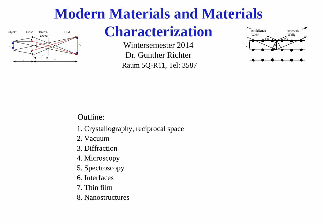
Outline:
1. Crystallography, reciprocal space
2. Vacuum
3. Diffraction
4. Microscopy
5. Spectroscopy
6. Interfaces
7. Thin film
8. Nanostructures
Modern Materials and Materials
Characterization Wintersemester 2014
Dr. Gunther Richter
Raum 5Q-R11, Tel: 3587
Objekt Linse Brenn- Bild
ebene
u v
f
U V d
einfallende
Welle
gebeugte
Welle
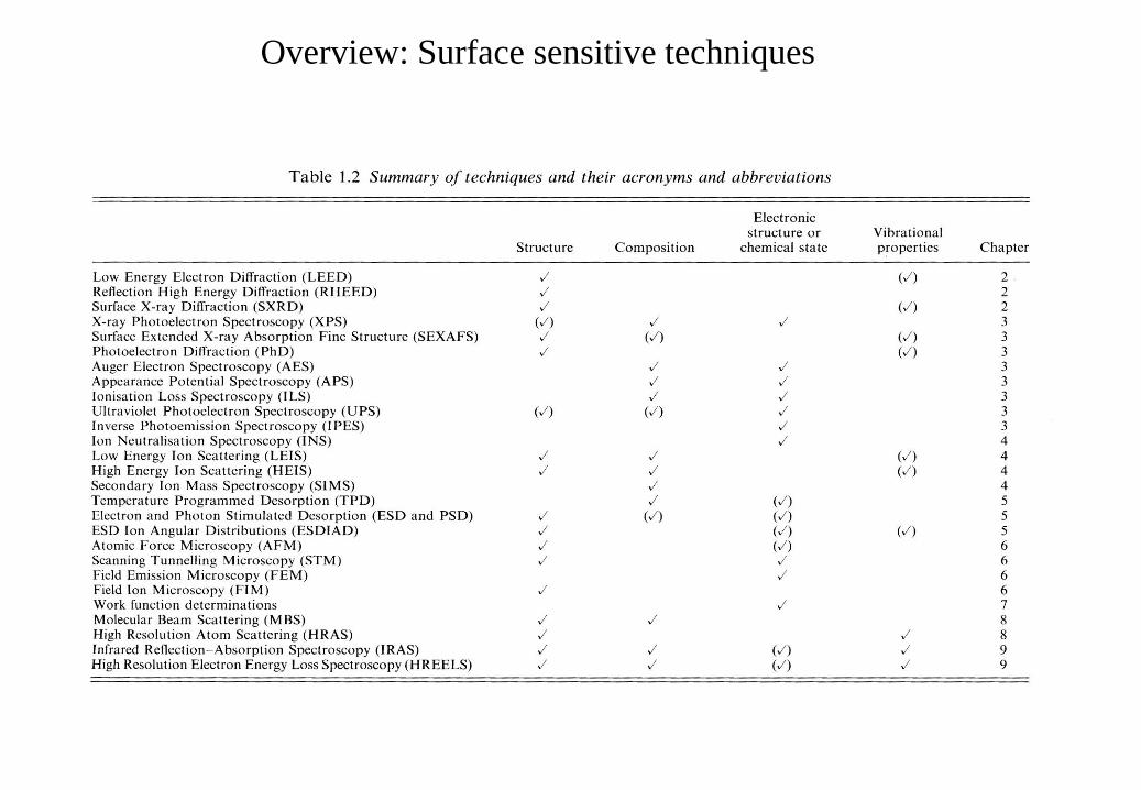
Overview: Surface sensitive techniques
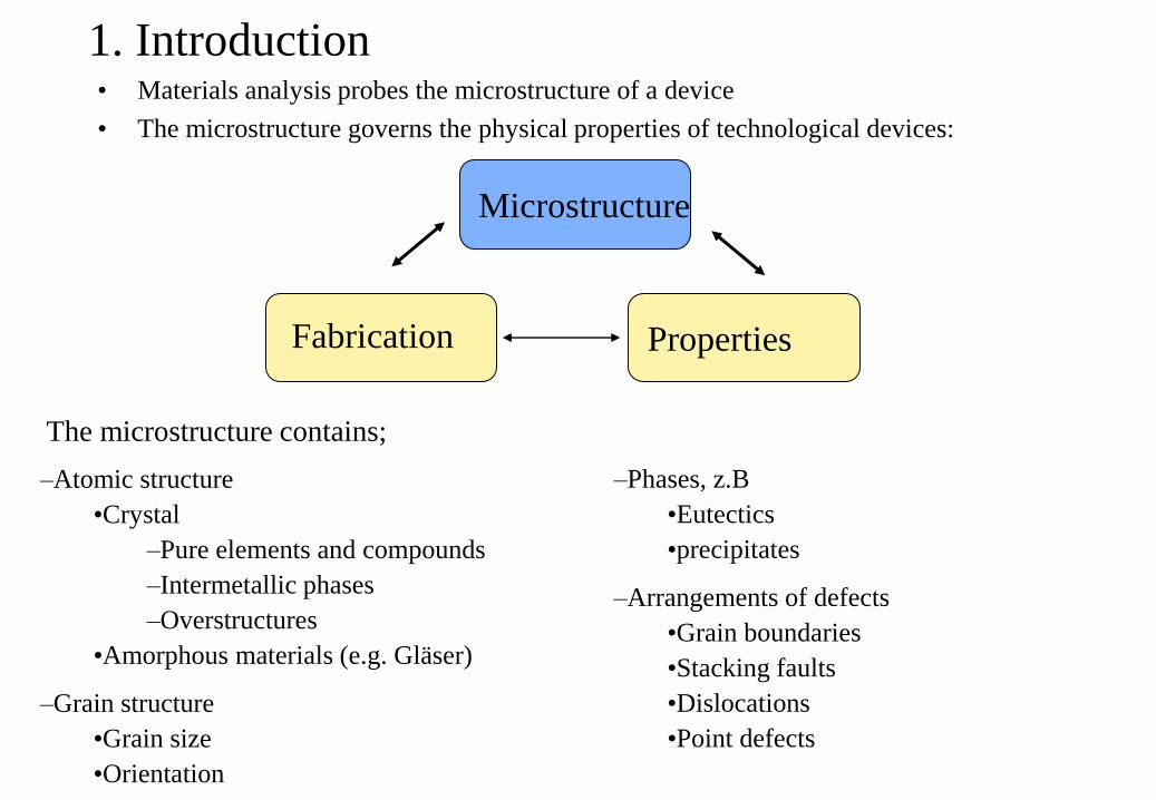
1. Introduction • Materials analysis probes the microstructure of a device
• The microstructure governs the physical properties of technological devices:
Microstructure
Fabrication Properties
–Phases, z.B
•Eutectics
•precipitates
–Arrangements of defects
•Grain boundaries
•Stacking faults
•Dislocations
•Point defects
–Atomic structure
•Crystal
–Pure elements and compounds
–Intermetallic phases
–Overstructures
•Amorphous materials (e.g. Gläser)
–Grain structure
•Grain size
•Orientation
The microstructure contains;
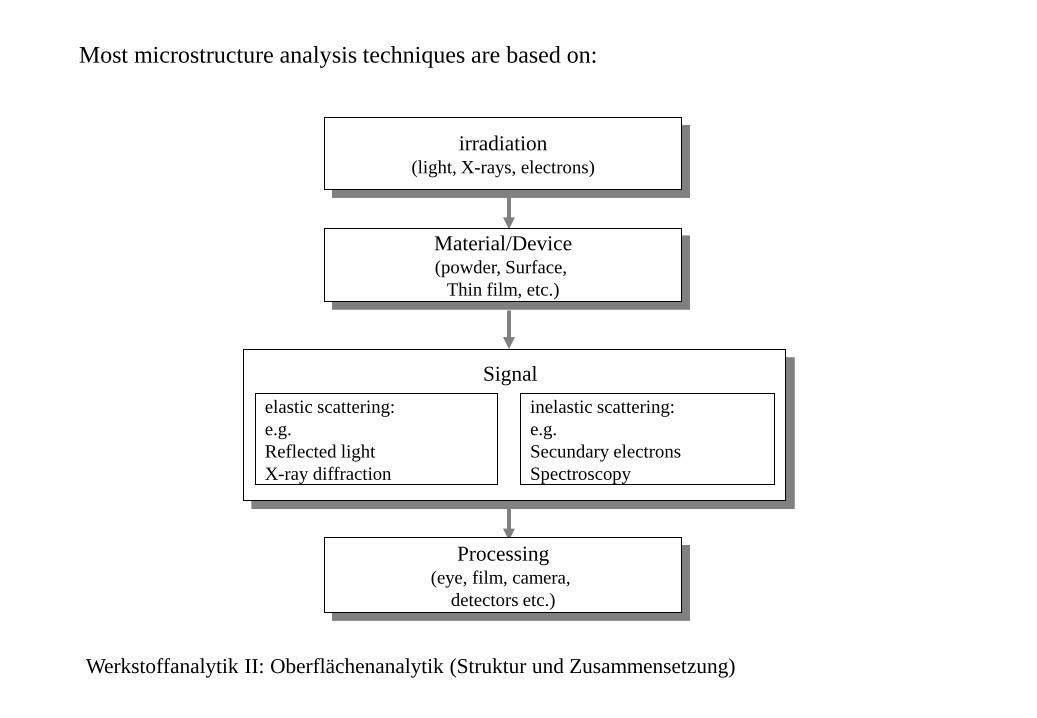
Most microstructure analysis techniques are based on:
irradiation (light, X-rays, electrons)
Material/Device (powder, Surface,
Thin film, etc.)
Processing (eye, film, camera,
detectors etc.)
elastic scattering:
e.g.
Reflected light
X-ray diffraction
inelastic scattering:
e.g.
Secundary electrons
Spectroscopy
Signal
Werkstoffanalytik II: Oberflächenanalytik (Struktur und Zusammensetzung)
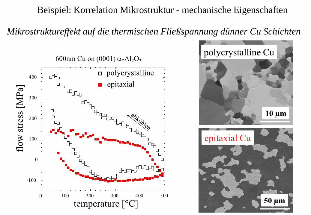
Beispiel: Korrelation Mikrostruktur - mechanische Eigenschaften
polycrystalline Cu
10 µm
600nm Cu on (0001) a-Al2O3
polycrystalline
epitaxial
-100
0
100
200
300
400
0 100 200 300 400 500
flow
str
ess
[MP
a]
temperature [°C]
epitaxial Cu
50 µm
Mikrostruktureffekt auf die thermischen Fließspannung dünner Cu Schichten
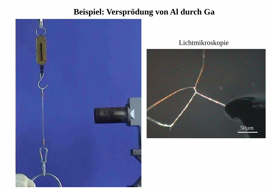
Beispiel: Versprödung von Al durch Ga
50µm
Lichtmikroskopie
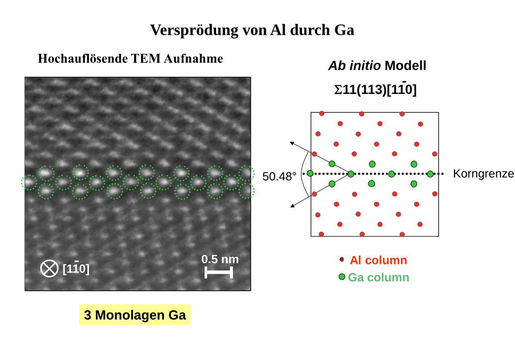
Versprödung von Al durch Ga
Korngrenze
Ab initio Modell
11(113)[110]
Al column
50.48°
Ga column
Hochauflösende TEM Aufnahme
3 Monolagen Ga
0.5 nm [110]
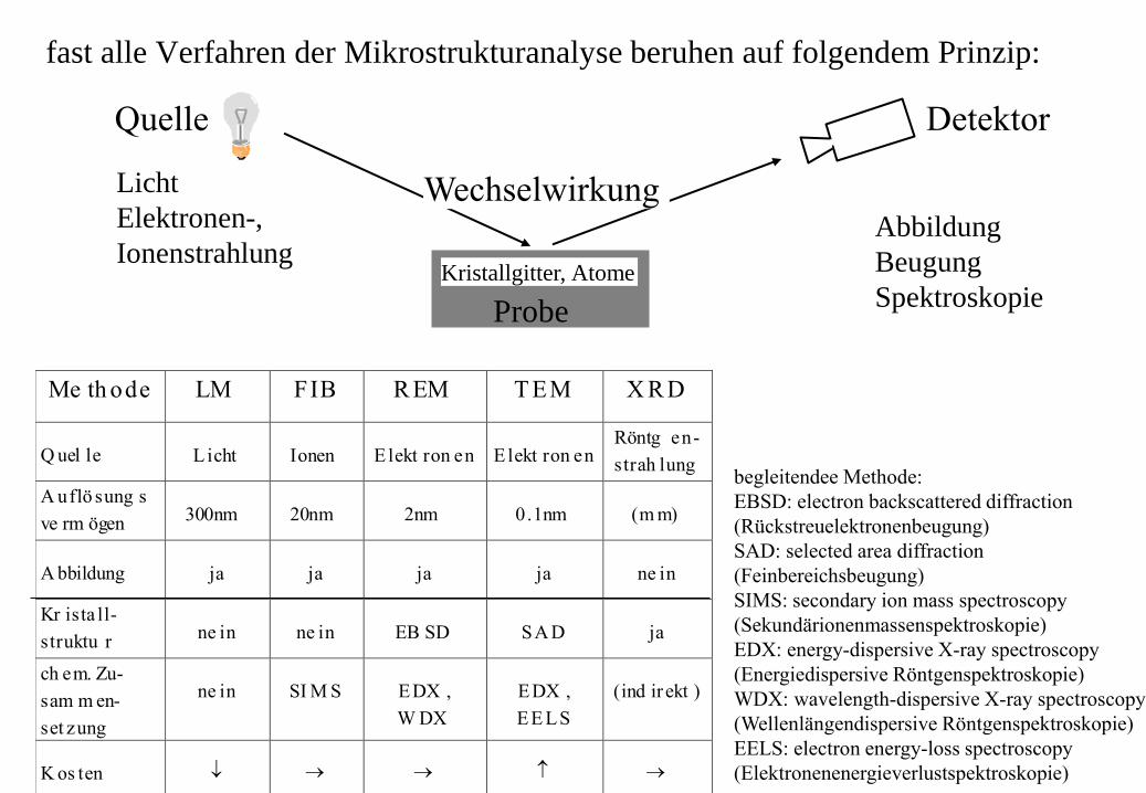
fast alle Verfahren der Mikrostrukturanalyse beruhen auf folgendem Prinzip:
Quelle Detektor
Probe
Abbildung
Beugung
Spektroskopie Kristallgitter, Atome
Wechselwirkung Licht
Elektronen-,
Ionenstrahlung
Me th ode LM FIB R EM T EM X R D
Q uel le L icht Ionen Elekt ron en Elekt ron enRöntg en-
strah lung
A uflö sung s
ve rm ögen300nm 20nm 2nm 0.1nm (m m)
A bbildung ja ja ja ja ne in
Kr ista ll-
struktu rne in ne in EB SD SA D ja
ch em. Zu-
sam m en-
set zung
ne in SI M S EDX ,
W DX
EDX ,
EE LS
(ind ir ekt )
K os ten
begleitendee Methode:
EBSD: electron backscattered diffraction
(Rückstreuelektronenbeugung)
SAD: selected area diffraction
(Feinbereichsbeugung)
SIMS: secondary ion mass spectroscopy
(Sekundärionenmassenspektroskopie)
EDX: energy-dispersive X-ray spectroscopy
(Energiedispersive Röntgenspektroskopie)
WDX: wavelength-dispersive X-ray spectroscopy
(Wellenlängendispersive Röntgenspektroskopie)
EELS: electron energy-loss spectroscopy
(Elektronenenergieverlustspektroskopie)
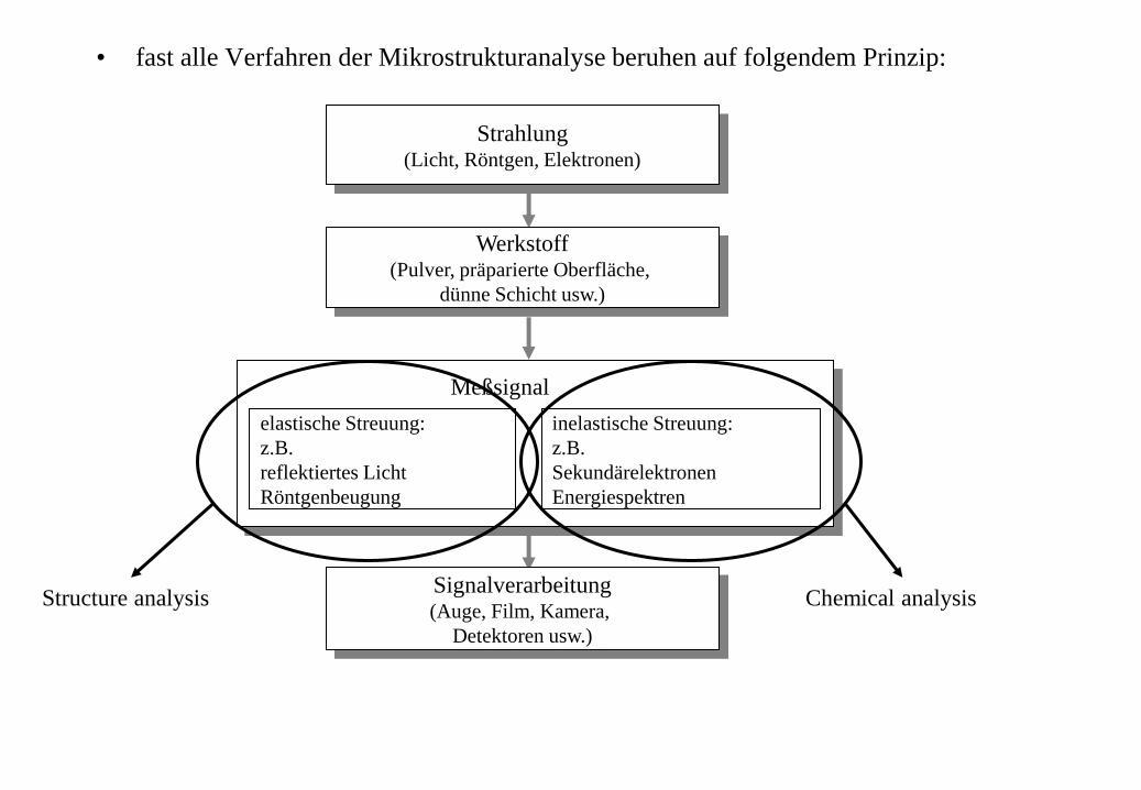
• fast alle Verfahren der Mikrostrukturanalyse beruhen auf folgendem Prinzip:
Strahlung (Licht, Röntgen, Elektronen)
Werkstoff (Pulver, präparierte Oberfläche,
dünne Schicht usw.)
Signalverarbeitung (Auge, Film, Kamera,
Detektoren usw.)
elastische Streuung:
z.B.
reflektiertes Licht
Röntgenbeugung
inelastische Streuung:
z.B.
Sekundärelektronen
Energiespektren
Meßsignal
Structure analysis Chemical analysis
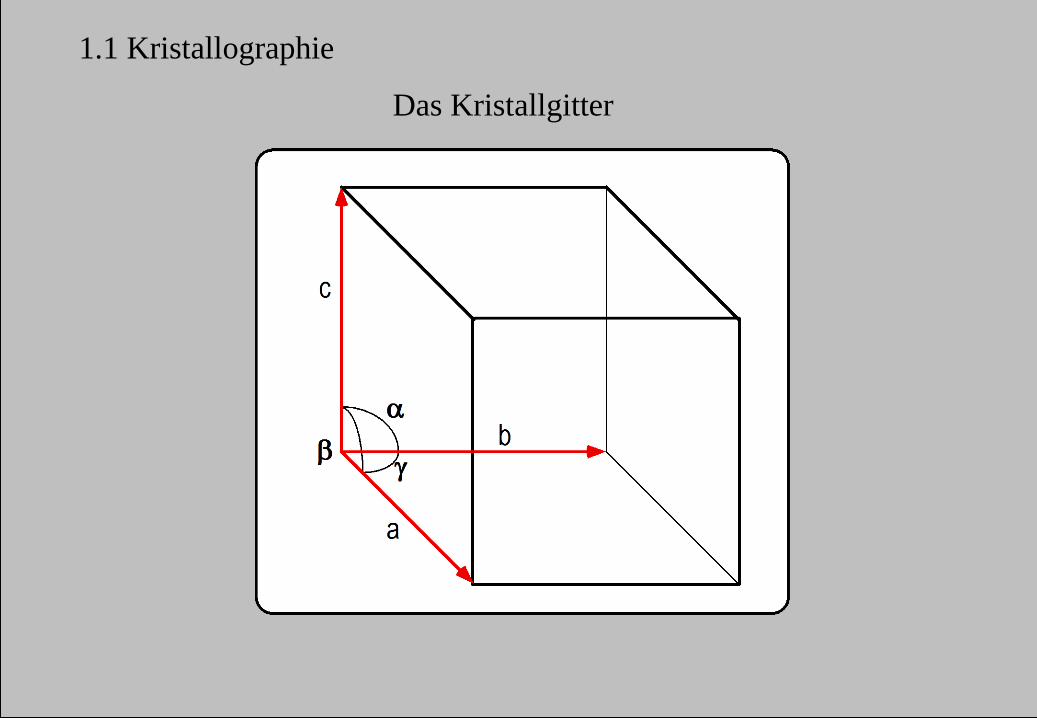
1.1 Kristallographie
Das Kristallgitter
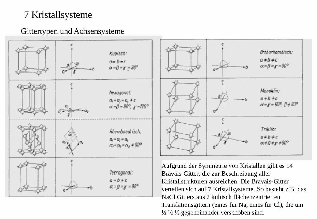
7 Kristallsysteme
Aufgrund der Symmetrie von Kristallen gibt es 14
Bravais-Gitter, die zur Beschreibung aller
Kristallstrukturen ausreichen. Die Bravais-Gitter
verteilen sich auf 7 Kristallsysteme. So besteht z.B. das
NaCl Gitters aus 2 kubisch flächenzentrierten
Translationsgittern (eines für Na, eines für Cl), die um
½ ½ ½ gegeneinander verschoben sind.
Gittertypen und Achsensysteme

1.2 Gittertypen (Bravais-Gitter)
System Primitivität Benennung Achsen/Winkelbedingunge
n
kubisch 1.) einfach-primitv
2.) zweifach-primitv
3.) vierfach-primitv
eckenbesetzt
raumzentriert
allseitig flächenzentriert
a = b = c, a = b = g = 90°
tetragonal 4.) einfach-primitv
5.) zweifach-primitv
eckenbesetzt
raumzentriert a = b c, a = b = g = 90°
hexagonal 6.) einfach-primitv
7.) dreifach-primitv
7'.) einfach-primitv
eckenbesetzt
2-fach raumzentriert
rhomboeder-eckenbesetzt
a = b /= c, a = 120°, g = 90°
rhombisch
8.) einfach-primitv
9.) zweifach-primitv
10.a) zweifach-primitv
10.b) zweifach-primitv
10.c) zweifach-primitv
11.) vierfach-primitv
eckenbesetzt
raumzentriert
(vorder-) flächenzentriert
(seiten-) flächenzentriert
basiszentriert
allseitig flächenzentriert
a b c, a = b = g = 90°
(rhomboedrisch) o. Abb. a = b = c, a = b = g 90°
monoklin 12.) einfach-primitv
13.) zweifach-primitv
eckenbesetzt
basiszentriert a b c, a = g = 90° b
triklin 14.) einfach-primitv eckenbesetzt a b c, a b g 90°
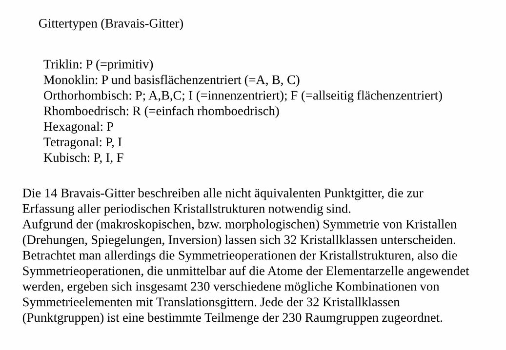
Gittertypen (Bravais-Gitter)
Die 14 Bravais-Gitter beschreiben alle nicht äquivalenten Punktgitter, die zur
Erfassung aller periodischen Kristallstrukturen notwendig sind.
Aufgrund der (makroskopischen, bzw. morphologischen) Symmetrie von Kristallen
(Drehungen, Spiegelungen, Inversion) lassen sich 32 Kristallklassen unterscheiden.
Betrachtet man allerdings die Symmetrieoperationen der Kristallstrukturen, also die
Symmetrieoperationen, die unmittelbar auf die Atome der Elementarzelle angewendet
werden, ergeben sich insgesamt 230 verschiedene mögliche Kombinationen von
Symmetrieelementen mit Translationsgittern. Jede der 32 Kristallklassen
(Punktgruppen) ist eine bestimmte Teilmenge der 230 Raumgruppen zugeordnet.
Triklin: P (=primitiv)
Monoklin: P und basisflächenzentriert (=A, B, C)
Orthorhombisch: P; A,B,C; I (=innenzentriert); F (=allseitig flächenzentriert)
Rhomboedrisch: R (=einfach rhomboedrisch)
Hexagonal: P
Tetragonal: P, I
Kubisch: P, I, F
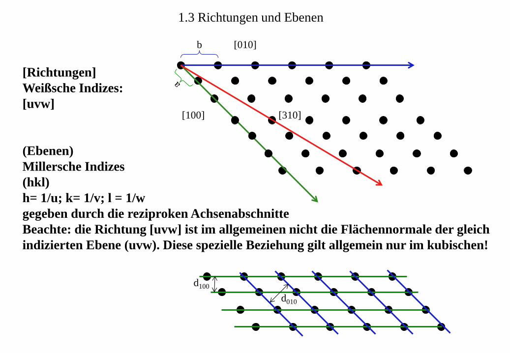
1.3 Richtungen und Ebenen
[100]
[010]
[310]
b
[Richtungen]
Weißsche Indizes:
[uvw]
(Ebenen)
Millersche Indizes
(hkl)
h= 1/u; k= 1/v; l = 1/w
gegeben durch die reziproken Achsenabschnitte
Beachte: die Richtung [uvw] ist im allgemeinen nicht die Flächennormale der gleich
indizierten Ebene (uvw). Diese spezielle Beziehung gilt allgemein nur im kubischen!
d100
d010
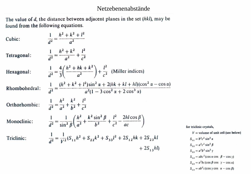
Netzebenenabstände
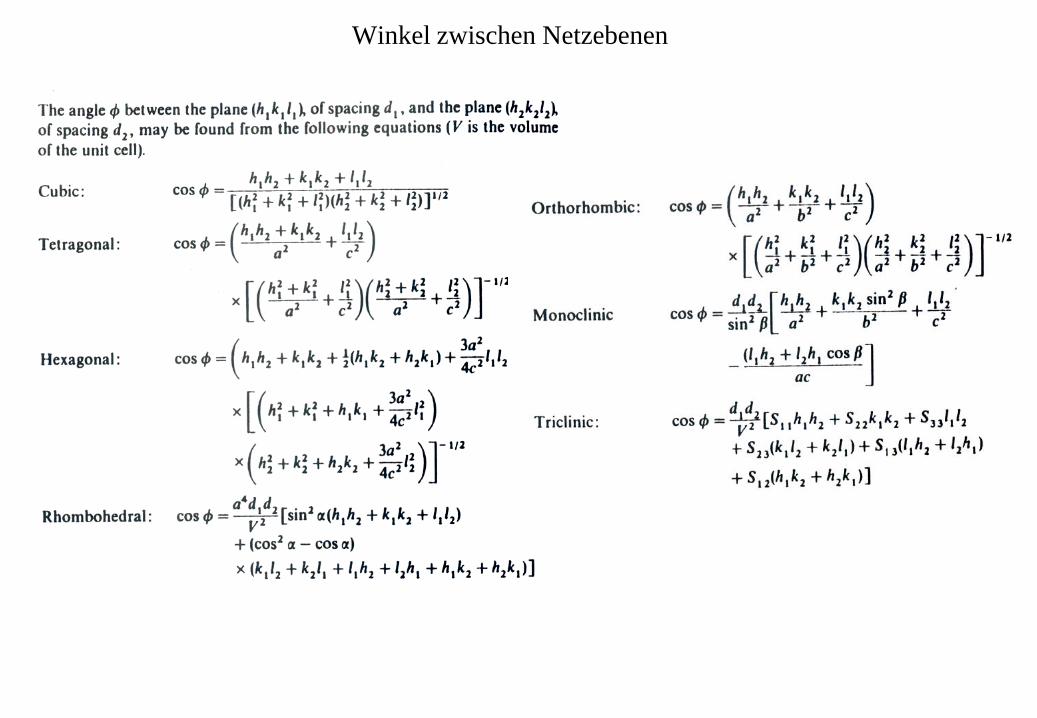
Winkel zwischen Netzebenen
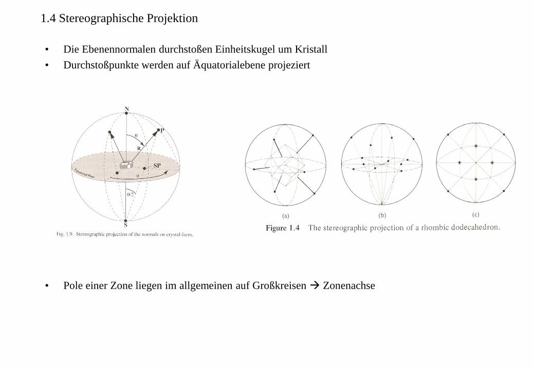
1.4 Stereographische Projektion
• Die Ebenennormalen durchstoßen Einheitskugel um Kristall
• Durchstoßpunkte werden auf Äquatorialebene projeziert
• Pole einer Zone liegen im allgemeinen auf Großkreisen Zonenachse
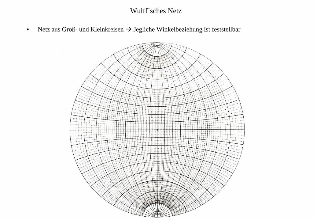
Wulff´sches Netz
• Netz aus Groß- und Kleinkreisen Jegliche Winkelbeziehung ist feststellbar
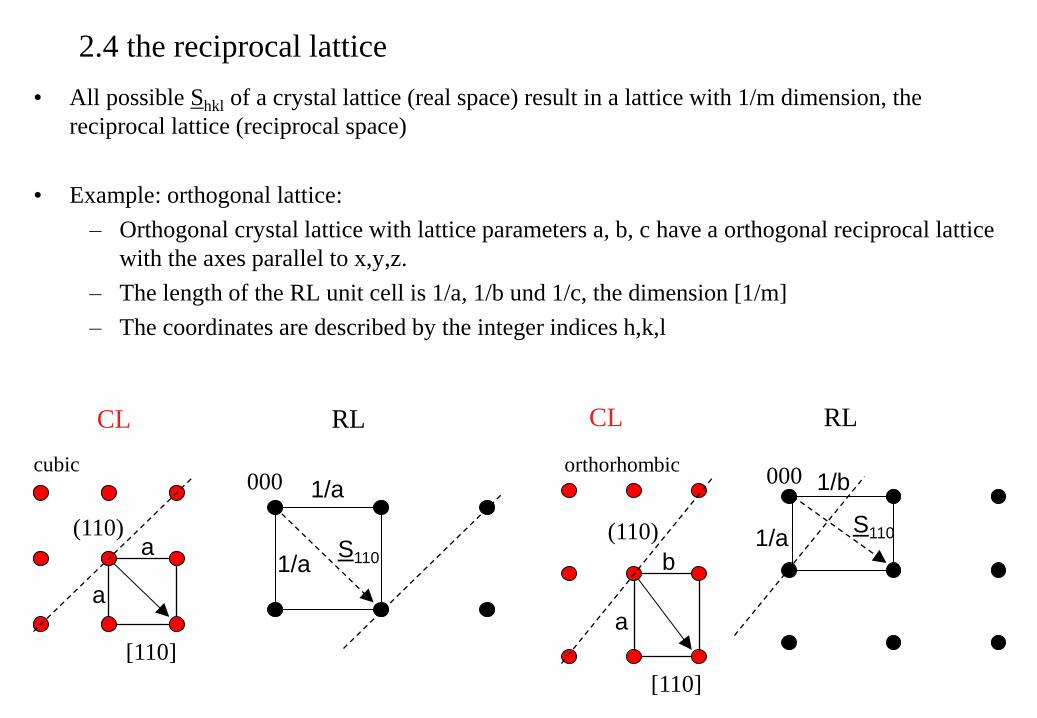
2.4 the reciprocal lattice
• All possible Shkl of a crystal lattice (real space) result in a lattice with 1/m dimension, the
reciprocal lattice (reciprocal space)
• Example: orthogonal lattice:
– Orthogonal crystal lattice with lattice parameters a, b, c have a orthogonal reciprocal lattice
with the axes parallel to x,y,z.
– The length of the RL unit cell is 1/a, 1/b und 1/c, the dimension [1/m]
– The coordinates are described by the integer indices h,k,l
CL RL
1/a
1/a
000
S110 a
a
(110)
[110]
cubic
b
a
(110)
[110]
1/b
1/a
000
S110
orthorhombic
CL RL
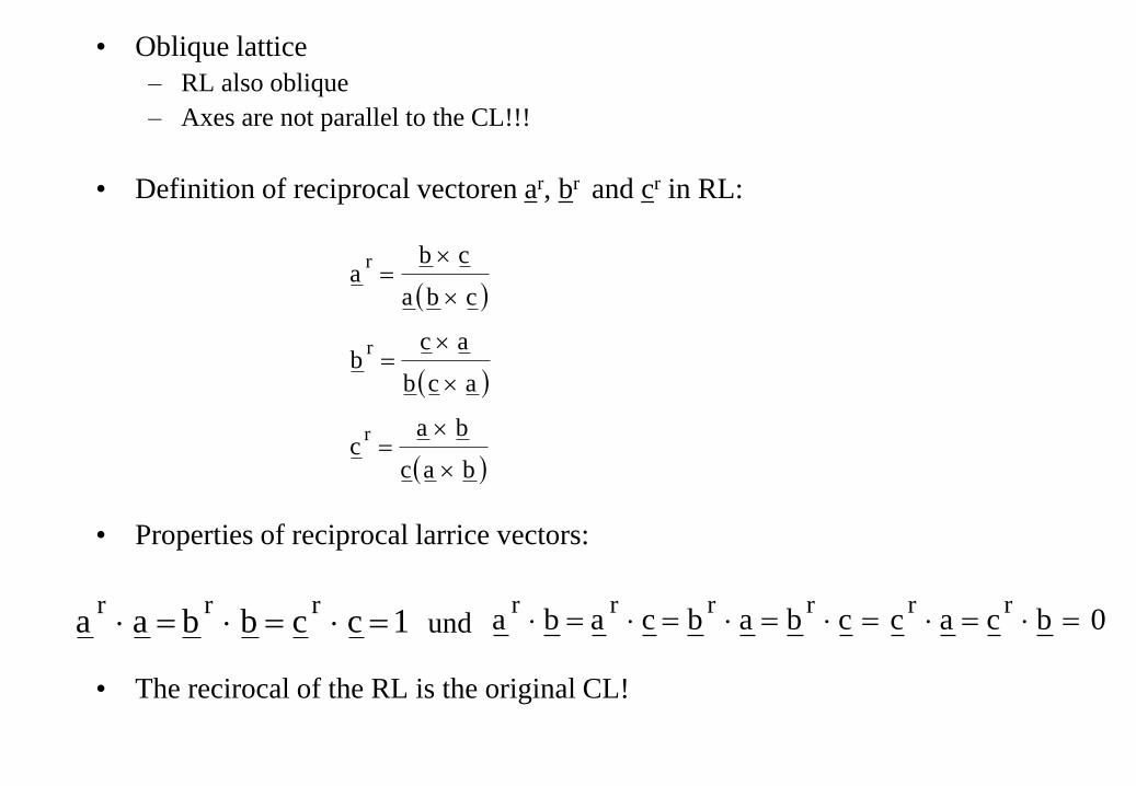
• Oblique lattice
– RL also oblique
– Axes are not parallel to the CL!!!
• Definition of reciprocal vectoren ar, br and cr in RL:
• Properties of reciprocal larrice vectors:
• The recirocal of the RL is the original CL!
bac
bac
acb
acb
cba
cba
r
r
r
1ccbbaarrr
0bcaccbabcabarrrrrr
und
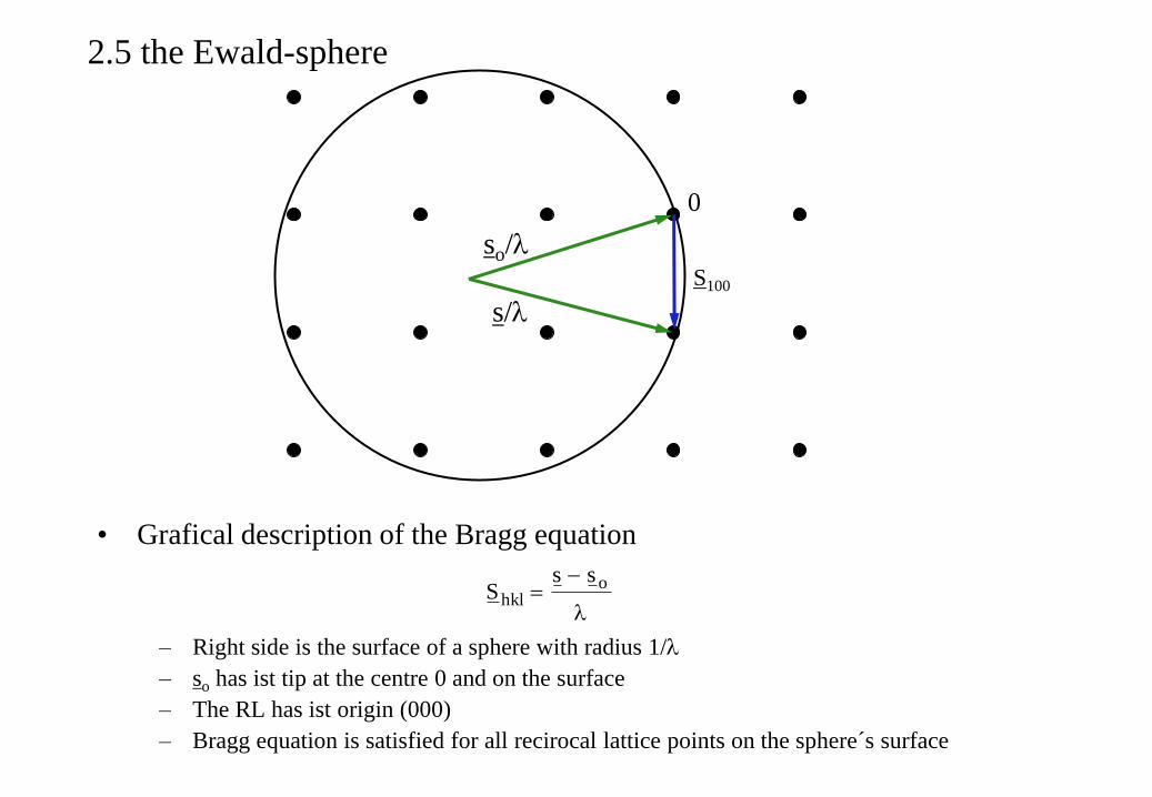
2.5 the Ewald-sphere
0
so/l
s/l
S100
• Grafical description of the Bragg equation
– Right side is the surface of a sphere with radius 1/l
– so has ist tip at the centre 0 and on the surface
– The RL has ist origin (000)
– Bragg equation is satisfied for all recirocal lattice points on the sphere´s surface
l
ohkl
ssS
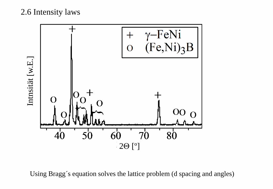
2.6 Intensity laws
Intn
sitä
t [w
.E.]
2Θ [º]
Using Bragg´s equation solves the lattice problem (d spacing and angles)
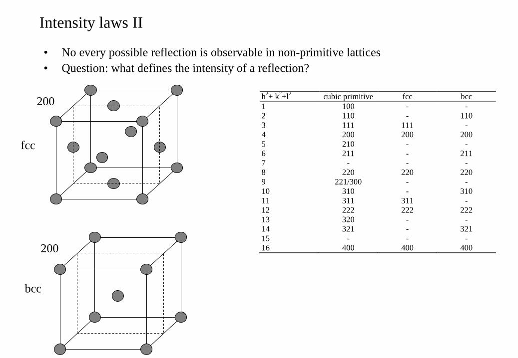
Intensity laws II
h2+ k
2+l
2 cubic primitive fcc bcc
1 100 - -
2 110 - 110
3 111 111 -
4 200 200 200
5 210 - -
6 211 - 211
7 - - -
8 220 220 220
9 221/300 - -
10 310 - 310
11 311 311 -
12 222 222 222
13 320 - -
14 321 - 321
15 - - -
16 400 400 400
• No every possible reflection is observable in non-primitive lattices
• Question: what defines the intensity of a reflection?
bcc
200
200
fcc
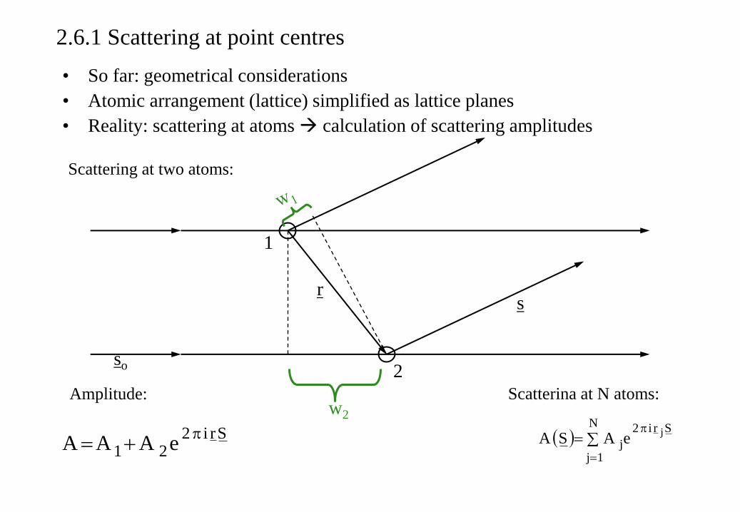
2.6.1 Scattering at point centres
• So far: geometrical considerations
• Atomic arrangement (lattice) simplified as lattice planes
• Reality: scattering at atoms calculation of scattering amplitudes
Scattering at two atoms:
2
w2
1
so
s r
Amplitude: Scatterina at N atoms:
Sri221 eAAA
N
1j
Sri2
jj
eASA
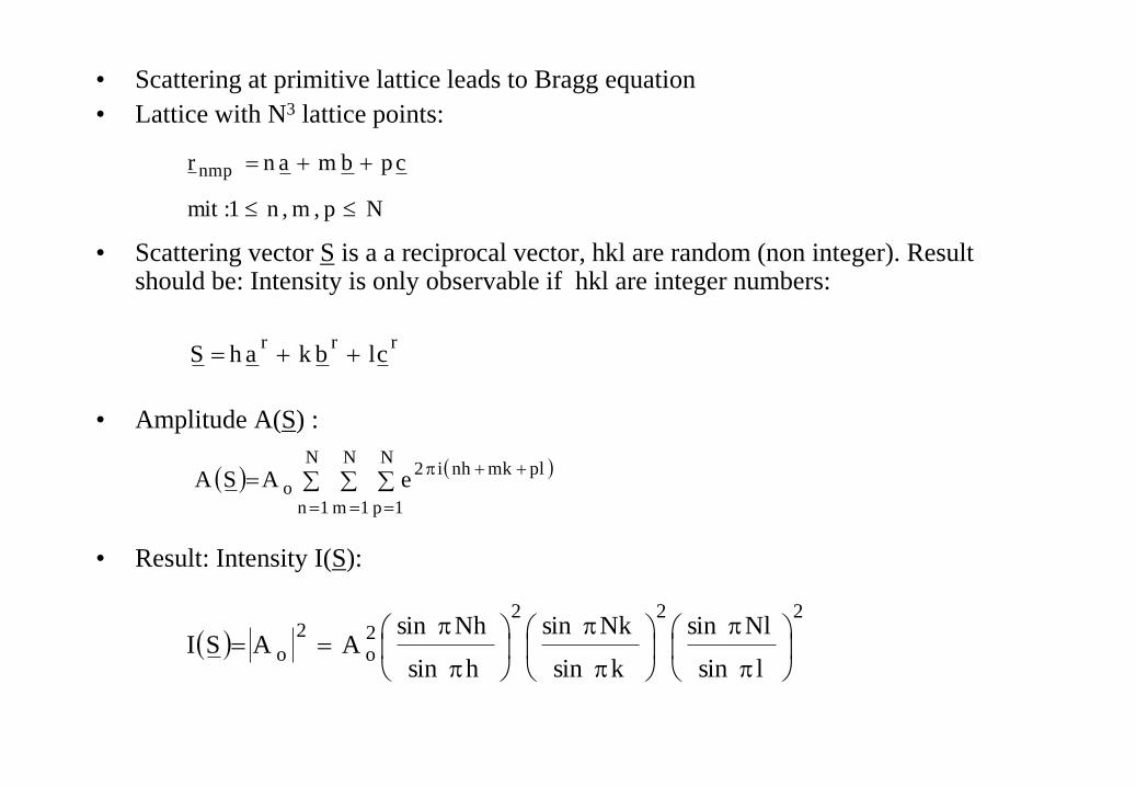
• Scattering at primitive lattice leads to Bragg equation
• Lattice with N3 lattice points:
• Scattering vector S is a a reciprocal vector, hkl are random (non integer). Result should be: Intensity is only observable if hkl are integer numbers:
• Amplitude A(S) :
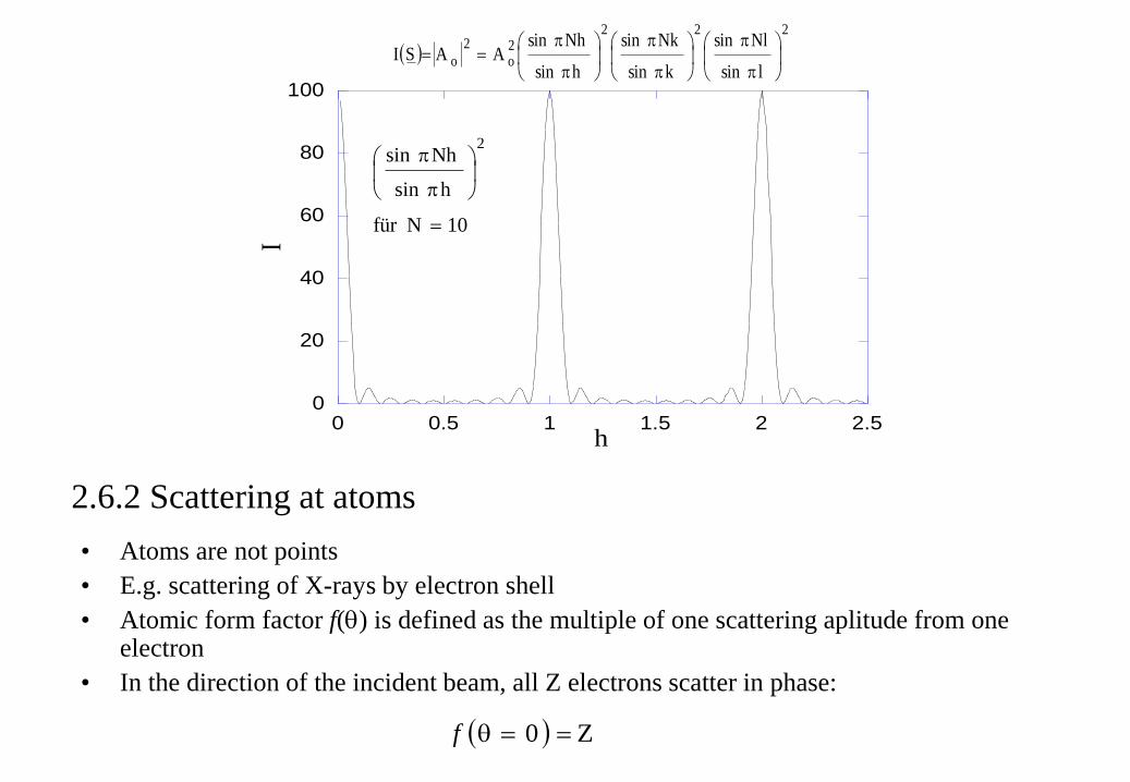
• Result: Intensity I(S):
Np,m,n1:mit
cpbmanr nmp
rrrclbkahS
N
1n
N
1m
N
1p
plmknhi2o eASA
222
2o
2
olsin
Nlsin
ksin
Nksin
hsin
NhsinAASI
0
20
40
60
80
100
0 0.5 1 1.5 2 2.5
I
h
222
2o
2
olsin
Nlsin
ksin
Nksin
hsin
NhsinAASI
10Nfür
hsin
Nhsin2
2.6.2 Scattering at atoms
• Atoms are not points
• E.g. scattering of X-rays by electron shell
• Atomic form factor f(q) is defined as the multiple of one scattering aplitude from one electron
• In the direction of the incident beam, all Z electrons scatter in phase:
Z0 qf
0
10
20
30
40
50
60
70
80
0 0.2 0.4 0.6 0.8 1
(2sin q/l
Neutrons
X-rays W
Al
Fe
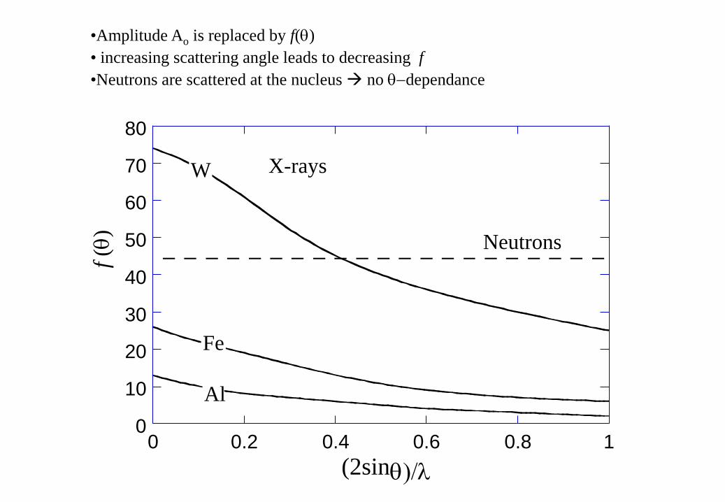
•Amplitude Ao is replaced by f(q)
• increasing scattering angle leads to decreasing f
•Neutrons are scattered at the nucleus no qdependance
f (q
)
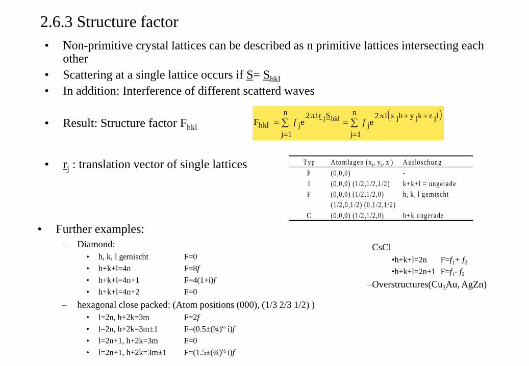
2.6.3 Structure factor
• Non-primitive crystal lattices can be described as n primitive lattices intersecting each other
• Scattering at a single lattice occurs if S= Shkl
• In addition: Interference of different scatterd waves
• Result: Structure factor Fhkl
• rj : translation vector of single lattices
Typ Atomla gen (x j, y j, z j) A uslöschung
P (0,0,0) -
I (0,0,0) (1/2,1 /2,1 /2) k+ k+l = ungera de
F (0,0,0) (1/2,1 /2,0)
(1/2,0,1 /2) (0,1/2,1/2)
h, k , l ge mischt
C (0,0,0) (1/2,1 /2,0) h+ k ungera de
• Further examples:
– Diamond:
• h, k, l gemischt F=0
• h+k+l=4n F=8f
• h+k+l=4n+1 F=4(1+i)f
• h+k+l=4n+2 F=0
– hexagonal close packed: (Atom positions (000), (1/3 2/3 1/2) )
• l=2n, h+2k=3m F=2f
• l=2n, h+2k=3m±1 F=(0.5±(¾)½ i)f
• l=2n+1, h+2k=3m F=0
• l=2n+1, h+2k=3m±1 F=(1.5±(¾)½ i)f
n
1j
lzkyhxi2
j
n
1j
Sri2
jhkljjjhklj
eeF ff
–CsCl
•h+k+l=2n F=f1+ f2
•h+k+l=2n+1 F=f1- f2
–Overstructures(Cu3Au, AgZn)
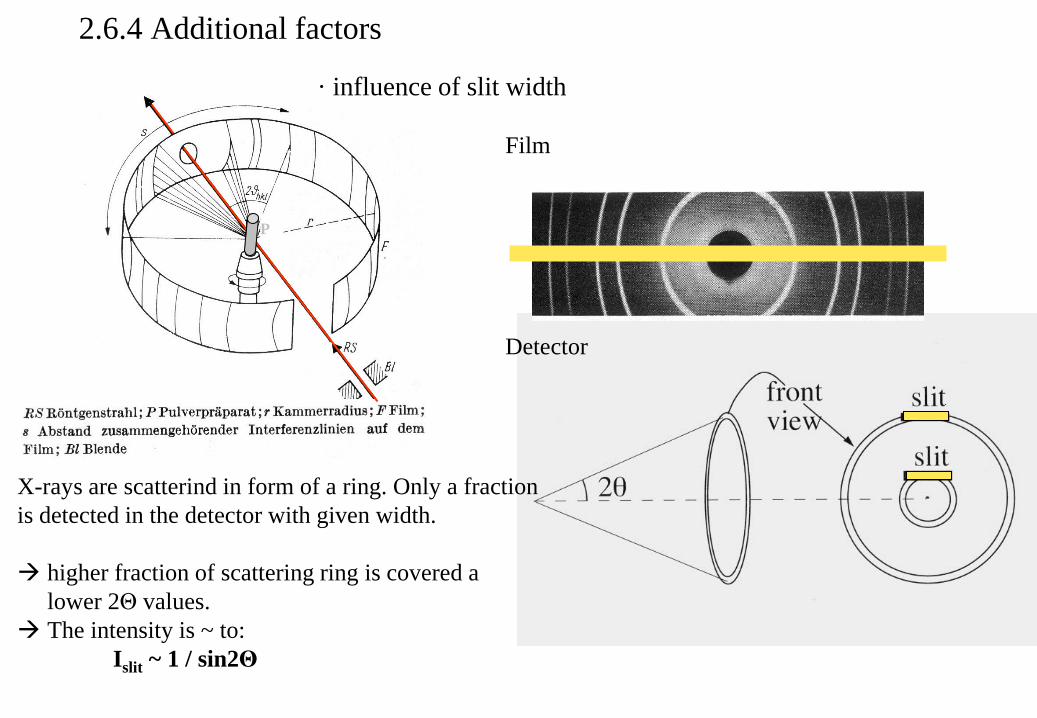
2.6.4 Additional factors
Film
Detector
P
X-rays are scatterind in form of a ring. Only a fraction
is detected in the detector with given width.
higher fraction of scattering ring is covered a
lower 2Θ values.
The intensity is ~ to:
Islit ~ 1 / sin2Θ
· influence of slit width
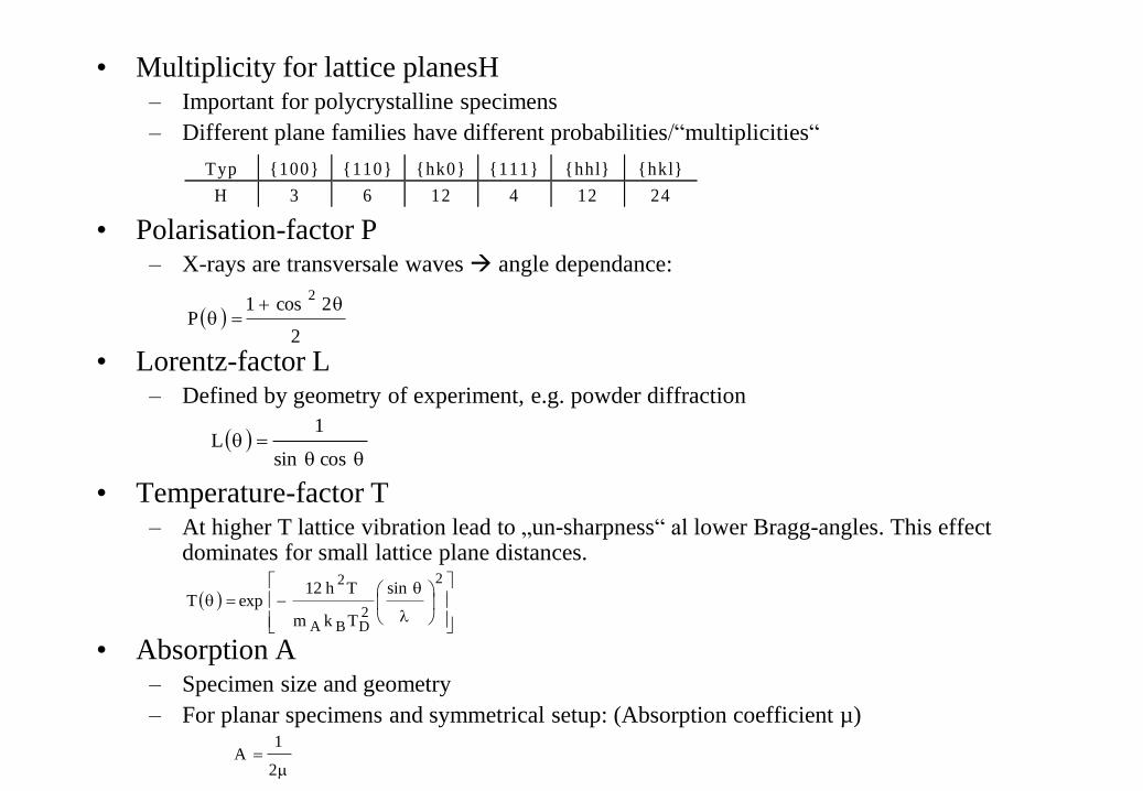
• Multiplicity for lattice planesH – Important for polycrystalline specimens
– Different plane families have different probabilities/“multiplicities“
• Polarisation-factor P – X-rays are transversale waves angle dependance:
• Lorentz-factor L – Defined by geometry of experiment, e.g. powder diffraction
• Temperature-factor T – At higher T lattice vibration lead to „un-sharpness“ al lower Bragg-angles. This effect
dominates for small lattice plane distances.
• Absorption A – Specimen size and geometry
– For planar specimens and symmetrical setup: (Absorption coefficient µ)
Typ {100} {110} {hk0} {111} {hhl} {hkl}
H 3 6 12 4 12 24
2
2cos1P
2q
q
qcossin
1L
l
2
2DBA
2sin
Tkm
Th12expT
2
1A
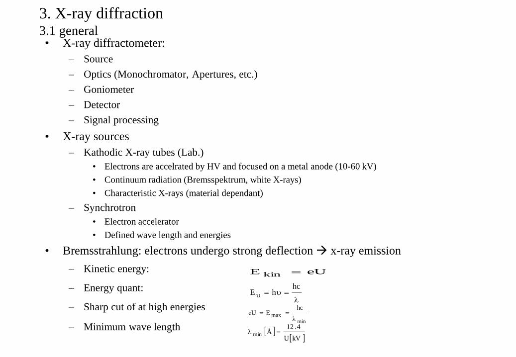
3. X-ray diffraction 3.1 general • X-ray diffractometer:
– Source
– Optics (Monochromator, Apertures, etc.)
– Goniometer
– Detector
– Signal processing
• X-ray sources
– Kathodic X-ray tubes (Lab.)
• Electrons are accelrated by HV and focused on a metal anode (10-60 kV)
• Continuum radiation (Bremsspektrum, white X-rays)
• Characteristic X-rays (material dependant)
– Synchrotron
• Electron accelerator
• Defined wave length and energies
• Bremsstrahlung: electrons undergo strong deflection x-ray emission
– Kinetic energy:
– Energy quant:
– Sharp cut of at high energies
– Minimum wave length
eUE kin
l
hchE
minmax
hcEeU
l
kVU
4.12Åmin l
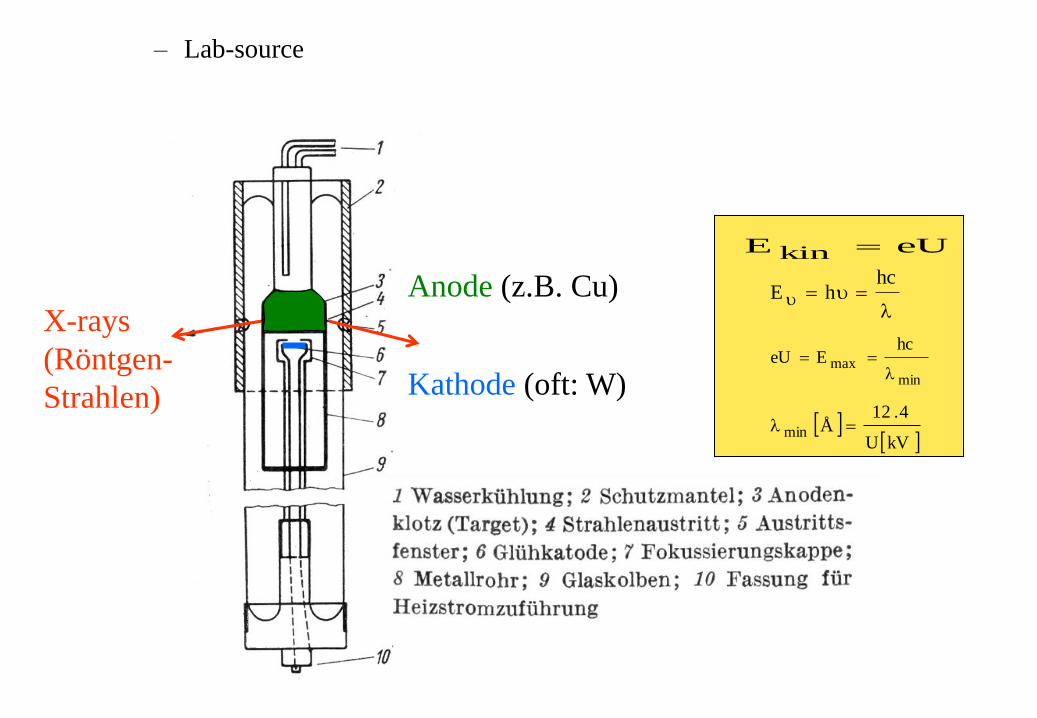
– Lab-source
X-rays
(Röntgen-
Strahlen)
Anode (z.B. Cu)
Kathode (oft: W)
eUE kin
l
hchE
minmax
hcEeU
l
kVU
4.12Åmin l
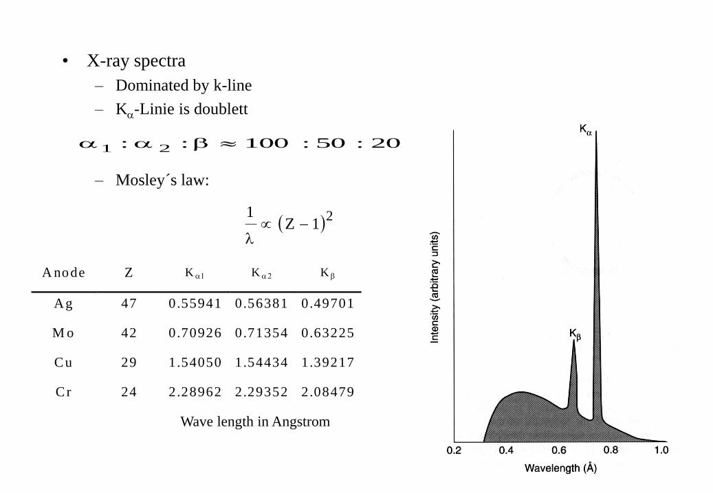
• X-ray spectra
– Dominated by k-line
– Ka-Linie is doublett
– Mosley´s law:
20:50:100:: 21 baa
21Z1
l
A node Z K a K a K b
Ag 47 0.55941 0.56381 0.49701
M o 42 0.70926 0.71354 0.63225
Cu 29 1.54050 1.54434 1.39217
Cr 24 2.28962 2.29352 2.08479
Wave length in Angstrom
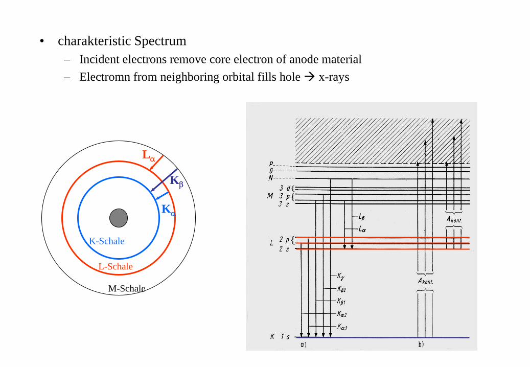
• charakteristic Spectrum
– Incident electrons remove core electron of anode material
– Electromn from neighboring orbital fills hole x-rays
K-Schale
L-Schale
M-Schale
Ka
Kb
La
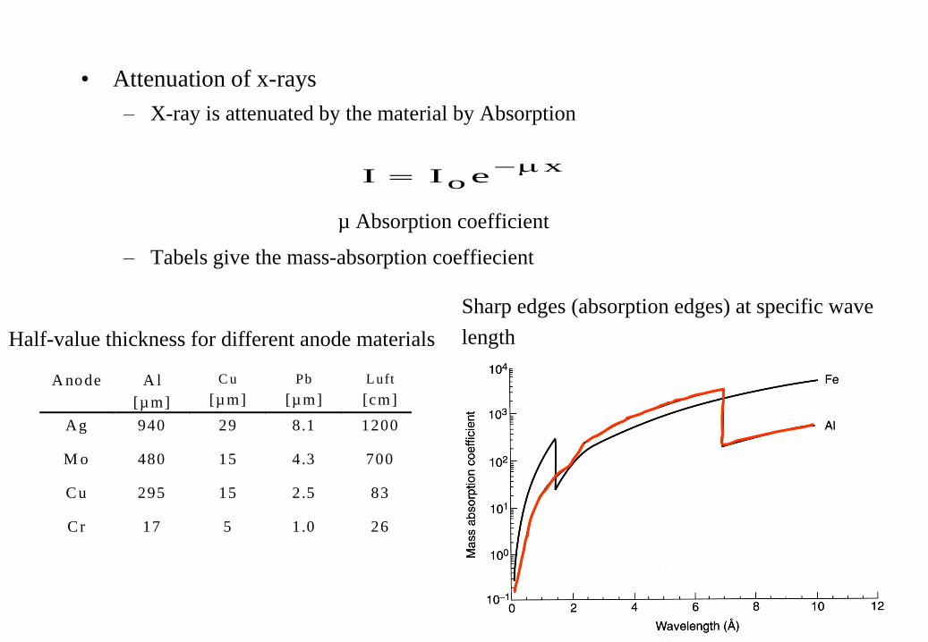
• Attenuation of x-rays
– X-ray is attenuated by the material by Absorption
µ Absorption coefficient
– Tabels give the mass-absorption coeffiecient
xoeII
A node A l
[µm]
C u
[µm]
Pb
[µm]
L uft
[cm]
Ag 940 29 8.1 1200
M o 480 15 4.3 700
C u 295 15 2.5 83
C r 17 5 1.0 26
Sharp edges (absorption edges) at specific wave
length Half-value thickness for different anode materials
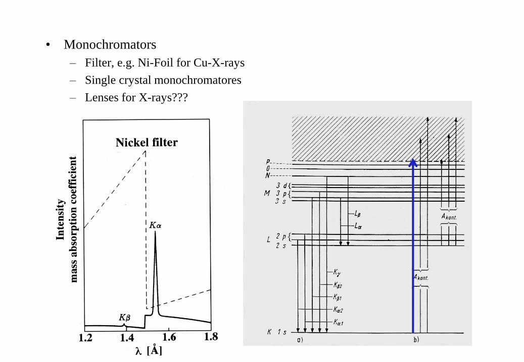
• Monochromators
– Filter, e.g. Ni-Foil for Cu-X-rays
– Single crystal monochromatores
– Lenses for X-rays???
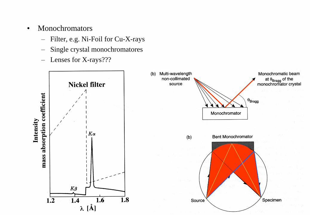
• Monochromators
– Filter, e.g. Ni-Foil for Cu-X-rays
– Single crystal monochromatores
– Lenses for X-rays???