tyre friction potential estimation by aligning torque …atuonone/files/tyre friction...
TRANSCRIPT
AALTO UNIVERSITY SCHOOL OF SCIENCE AND TECHNOLOGY Faculty of Engineering and Architecture Department of Engineering Design and Production
Mika Matilainen
Tyre Friction Potential Estimation by
Aligning Torque and Lateral Force Information
Thesis submitted in partial fulfilment of the requirements for the degree of
Master of Science in Technology.
Espoo, November 24, 2010
Supervisor Professor Matti Juhala Thesis Instructor Ari Tuononen Doctor of Science (Tech.)
2
AALTO UNIVERSITY SCHOOL OF SCIENCE AND TECHNOLOGY PO Box 11000, FI-00076 AALTO http://www.aalto.fi
ABSTRACT OF THE MASTER’S THESIS
Author: Mika Matilainen
Title: Tyre Friction Potential Estimation by Aligning Torque and Lateral Force Information
Faculty: Faculty of Engineering and Architecture
Department: Department of Engineering Design and Production
Professorship: Vehicle Engineering Code: Kon-16
Supervisor: Professor Matti Juhala
Instructor(s): Ari Tuononen Doctor of Science (Tech.)
Abstract:
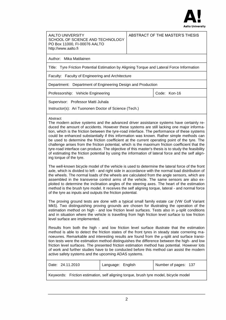
The modern active systems and the advanced driver assistance systems have certainly re-duced the amount of accidents. However these systems are still lacking one major informa-tion, which is the friction between the tyre-road interface. The performance of these systems could be enhanced substantially if this information was known. Rather simple methods can be used to determine the friction coefficient at the current operating point of the tyre. The challenge arises from the friction potential, which is the maximum friction coefficient that the tyre-road interface can produce. The objective of this master's thesis is to study the feasibility of estimating the friction potential by using the information of lateral force and the self align-ing torque of the tyre. The well-known bicycle model of the vehicle is used to determine the lateral force of the front axle, which is divided to left - and right side in accordance with the normal load distribution of the wheels. The normal loads of the wheels are calculated from the angle sensors, which are assembled in the transverse control arms of the vehicle. The same sensors are also ex-ploited to determine the inclination angles of the steering axes. The heart of the estimation method is the brush tyre model. It receives the self aligning torque, lateral - and normal force of the tyre as inputs and outputs the friction potential. The proving ground tests are done with a typical small family estate car (VW Golf Variant Mk5). Two distinguishing proving grounds are chosen for illustrating the operation of the
estimation method on high - and low friction level surfaces. Tests also in μ-split conditions and in situation where the vehicle is travelling from high friction level surface to low friction level surface are implemented. Results from both the high - and low friction level surface illustrate that the estimation method is able to detect the friction states of the front tyres in steady state cornering ma-
noeuvres. Remarkable and interesting results are found from the μ-split and surface transi-tion tests were the estimation method distinguishes the difference between the high- and low friction level surfaces. The presented friction estimation method has potential. However lots of work and further studies have to be conducted before this method can assist the modern active safety systems and the upcoming ADAS systems.
Date: 24.11.2010 Language: English Number of pages: 137
Keywords: Friction estimation, self aligning torque, brush tyre model, bicycle model
3
AALTO-YLIOPISTO TEKNILLINEN KORKEAKOULU PL 11000, 00076 Aalto http://www.aalto.fi
DIPLOMITYÖN TIIVISTELMÄ
Tekijä: Mika Matilainen
Työn nimi: Renkaan kitkapotentiaalin arvioiminen palauttavan momentin ja sivuttaisvoiman avulla
Tiedekunta Insinööritieteiden ja arkkitehtuurin tiedekunta
Laitos: Koneenrakennustekniikan laitos
Professuuri: Auto- ja työkonetekniikka Koodi: Kon-16
Työn valvoja: Professori Matti Juhala
Työn ohjaaja(t): Tekniikan tohtori Ari Tuononen
Tiivistelmä:
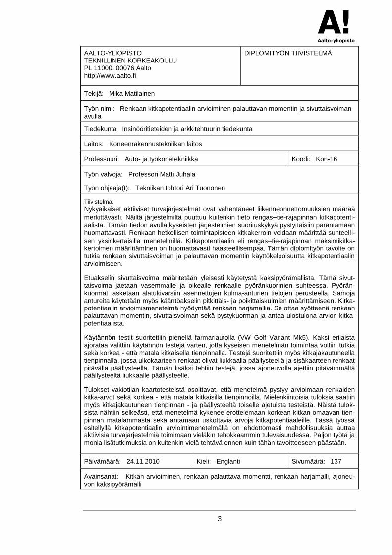
Nykyaikaiset aktiiviset turvajärjestelmät ovat vähentäneet liikenneonnettomuuksien määrää
merkittävästi. Näiltä järjestelmiltä puuttuu kuitenkin tieto rengas–tie-rajapinnan kitkapotenti-aalista. Tämän tiedon avulla kyseisten järjestelmien suorituskykyä pystyttäisiin parantamaan huomattavasti. Renkaan hetkellisen toimintapisteen kitkakerroin voidaan määrittää suhteelli-
sen yksinkertaisilla menetelmillä. Kitkapotentiaalin eli rengas–tie-rajapinnan maksimikitka-kertoimen määrittäminen on huomattavasti haasteellisempaa. Tämän diplomityön tavoite on tutkia renkaan sivuttaisvoiman ja palauttavan momentin käyttökelpoisuutta kitkapotentiaalin arvioimiseen.
Etuakselin sivuttaisvoima määritetään yleisesti käytetystä kaksipyörämallista. Tämä sivut-taisvoima jaetaan vasemmalle ja oikealle renkaalle pyöränkuormien suhteessa. Pyörän-kuormat lasketaan alatukivarsiin asennettujen kulma-anturien tietojen perusteella. Samoja antureita käytetään myös kääntöakselin pitkittäis- ja poikittaiskulmien määrittämiseen. Kitka-potentiaalin arvioimismenetelmä hyödyntää renkaan harjamallia. Se ottaa syötteenä renkaan palauttavan momentin, sivuttaisvoiman sekä pystykuorman ja antaa ulostulona arvion kitka-potentiaalista.
Käytännön testit suoritettiin pienellä farmariautolla (VW Golf Variant Mk5). Kaksi erilaista ajorataa valittiin käytännön testejä varten, jotta kyseisen menetelmän toimintaa voitiin tutkia sekä korkea - että matala kitkaisella tienpinnalla. Testejä suoritettiin myös kitkajakautuneella tienpinnalla, jossa ulkokaarteen renkaat olivat liukkaalla päällysteellä ja sisäkaarteen renkaat pitävällä päällysteellä. Tämän lisäksi tehtiin testejä, jossa ajoneuvolla ajettiin pitävämmältä päällysteeltä liukkaalle päällysteelle.
Tulokset vakiotilan kaartotesteistä osoittavat, että menetelmä pystyy arvioimaan renkaiden kitka-arvot sekä korkea - että matala kitkaisilla tienpinnoilla. Mielenkiintoisia tuloksia saatiin myös kitkajakautuneen tienpinnan - ja päällysteeltä toiselle ajetuista testeistä. Näistä tulok-sista nähtiin selkeästi, että menetelmä kykenee erottelemaan korkean kitkan omaavan tien-pinnan matalammasta sekä antamaan uskottavia arvoja kitkapotentiaaleille. Tässä työssä esitellyllä kitkapotentiaalin arviointimenetelmällä on ehdottomasti mahdollisuuksia auttaa aktiivisia turvajärjestelmiä toimimaan vieläkin tehokkaammin tulevaisuudessa. Paljon työtä ja monia lisätutkimuksia on kuitenkin vielä tehtävä ennen kuin tähän tavoitteeseen päästään.
Päivämäärä: 24.11.2010 Kieli: Englanti Sivumäärä: 137
Avainsanat: Kitkan arvioiminen, renkaan palauttava momentti, renkaan harjamalli, ajoneu-von kaksipyörämalli

Acknowledgements
4
Acknowledgements
This master’s thesis was done in Aalto University School of Science and Tech-
nology. First of all I want to give my appreciations to Henry Ford Foundation for
providing me a scholarship to carry out this interesting study.
Special thanks are reserved for Professor Matti Juhala, researcher Ari Tuononen
and senior laboratory manager Panu Sainio. These appreciations aren’t only for
encouraging and supporting me throughout my master’s thesis, but also for giv-
ing me interesting working possibilities at the Laboratory of Automotive Engineer-
ing. My compliments go also to senior laboratory technicians Pekka Martelius
and Keijo Kallio, who helped me with the sensor calibrations and mounting of the
sensor equipment to the research vehicle. Thanks also to Professor Petri Kuos-
manen for reading my almost finished master’s thesis with a short notice and
giving valuable comments about it.
Thanks to all fellow master’s thesis workers at the open-plan office for keeping
the atmosphere relaxed and pleasant.
Finally but certainly not for least I want to thank my parents, who have been sup-
porting me throughout my studies.
Espoo November 24, 2010
Mika Matilainen
Table of Contents
5
Table of Contents
ABSTRACT OF THE MASTER’S THESIS .......................................................... 2
DIPLOMITYÖN TIIVISTELMÄ ............................................................................. 3
Acknowledgements ............................................................................................. 4
Table of Contents ................................................................................................ 5
Symbols and Definitions ...................................................................................... 9
Abbreviations .....................................................................................................12
1 Introduction .................................................................................................13
1.1 Motivation and Background ..................................................................13
1.2 Problem Statement ..............................................................................17
1.3 Outline .................................................................................................19
1.4 Main Results ........................................................................................20
2 The Rubber-Road Interface: Phenomena Involved in Friction .....................21
2.1 Introduction ..........................................................................................21
2.2 Characteristics of Rubber .....................................................................21
2.2.1 Visco-elastic Behaviour .................................................................21
2.2.2 Influence of Stress Frequency .......................................................24
2.2.3 Influence of Temperature ..............................................................25
2.3 Characteristics of Road Surfaces .........................................................26
2.3.1 Texture..........................................................................................26
2.3.2 Influence of Surface Conditions ....................................................29
2.4 Friction Mechanisms ............................................................................31
2.4.1 Adhesion .......................................................................................31
2.4.2 Hysteresis .....................................................................................32
2.5 Conclusions of this Chapter .................................................................33

Table of Contents
6
3 Background and Theory of Friction Estimation ............................................34
3.1 Introduction ..........................................................................................34
3.2 Friction Coefficient ...............................................................................34
3.2.1 Definition .......................................................................................34
3.2.2 Terminology ..................................................................................37
3.3 Classification of Friction Estimation Methods .......................................39
3.3.1 Direct Methods ..............................................................................39
3.3.2 Indirect Methods ...........................................................................40
3.4 Previous Studies ..................................................................................41
3.5 Conclusions of this Chapter .................................................................42
4 Research Vehicle and Sensor Equipment ...................................................44
4.1 Introduction ..........................................................................................44
4.2 Front Suspension Geometry ................................................................45
4.2.1 Overview .......................................................................................45
4.2.2 Steering Axis .................................................................................47
4.2.3 Caster Angle .................................................................................47
4.2.4 Kingpin Inclination Angle ...............................................................51
4.2.5 Camber Angle ...............................................................................52
4.3 Steering System ...................................................................................54
4.3.1 Overview .......................................................................................54
4.3.2 Forces and Torques ......................................................................55
4.3.3 Evaluation of the Force Lever Arm ................................................57
4.4 Sensor Equipment................................................................................59
4.4.1 Overview .......................................................................................59
4.4.2 Piezoelectric Force Sensor ...........................................................60
4.4.3 Hall Effect Angle Sensor ...............................................................67
4.4.4 Two-Axis Optical Velocity and Slip Angle Sensor ..........................71
4.5 Conclusions of this Chapter .................................................................72
Table of Contents
7
5 Proving Grounds and Experimental Tests ...................................................74
5.1 Introduction ..........................................................................................74
5.2 Proving Ground of Nokian Tyres ..........................................................74
5.2.1 Overview .......................................................................................74
5.2.2 Experimental Tests .......................................................................75
5.3 Test Driving Track of Uudenmaan Ajoharjoitteluradat ..........................77
5.3.1 Overview .......................................................................................77
5.3.2 Experimental Tests .......................................................................78
5.4 Conclusions of this Chapter .................................................................80
6 Friction Estimation Method ..........................................................................81
6.1 Introduction ..........................................................................................81
6.2 The Bicycle Model ................................................................................81
6.2.1 Definition and Assumptions ...........................................................81
6.2.2 Equations of Motion ......................................................................82
6.2.3 Lateral Tyre Forces and Slip Angles .............................................83
6.3 The Brush Tyre Model ..........................................................................86
6.3.1 Definition and Assumptions ...........................................................86
6.3.2 Determination of Normal Load Distribution and Contact Length ....88
6.3.3 Complete Adhesion .......................................................................90
6.3.4 Adhesion and Sliding ....................................................................91
6.3.5 Complete sliding ...........................................................................93
6.4 Friction Estimation in Pure Lateral Slip Situation ..................................94
6.4.1 Principle ........................................................................................94
6.4.2 Requirements and Limitations .......................................................97
6.4.3 Proof of Concept ......................................................................... 101
6.4.4 Implementation ........................................................................... 102
6.5 Conclusions of this Chapter ............................................................... 103
Table of Contents
8
7 Proving Ground Results and Discussion ................................................... 105
7.1 Introduction ........................................................................................ 105
7.2 Steady-State Cornering ...................................................................... 105
7.2.1 High Friction Level Road Surface ................................................ 105
7.2.2 Low Friction Level Road Surface................................................. 109
7.2.3 -split Road Surface ................................................................... 113
7.3 Ramp Steer from High - to Low Friction Level Road Surface ............. 117
7.4 Conclusion of this Chapter ................................................................. 121
8 Conclusions and Recommendations ......................................................... 123
Bibliography ..................................................................................................... 126
Appendix A1: Vehicle and tyre parameters ....................................................... 130
Appendix A2: Contact pressure distribution and contact patch length .............. 131
Symbols and Definitions
9
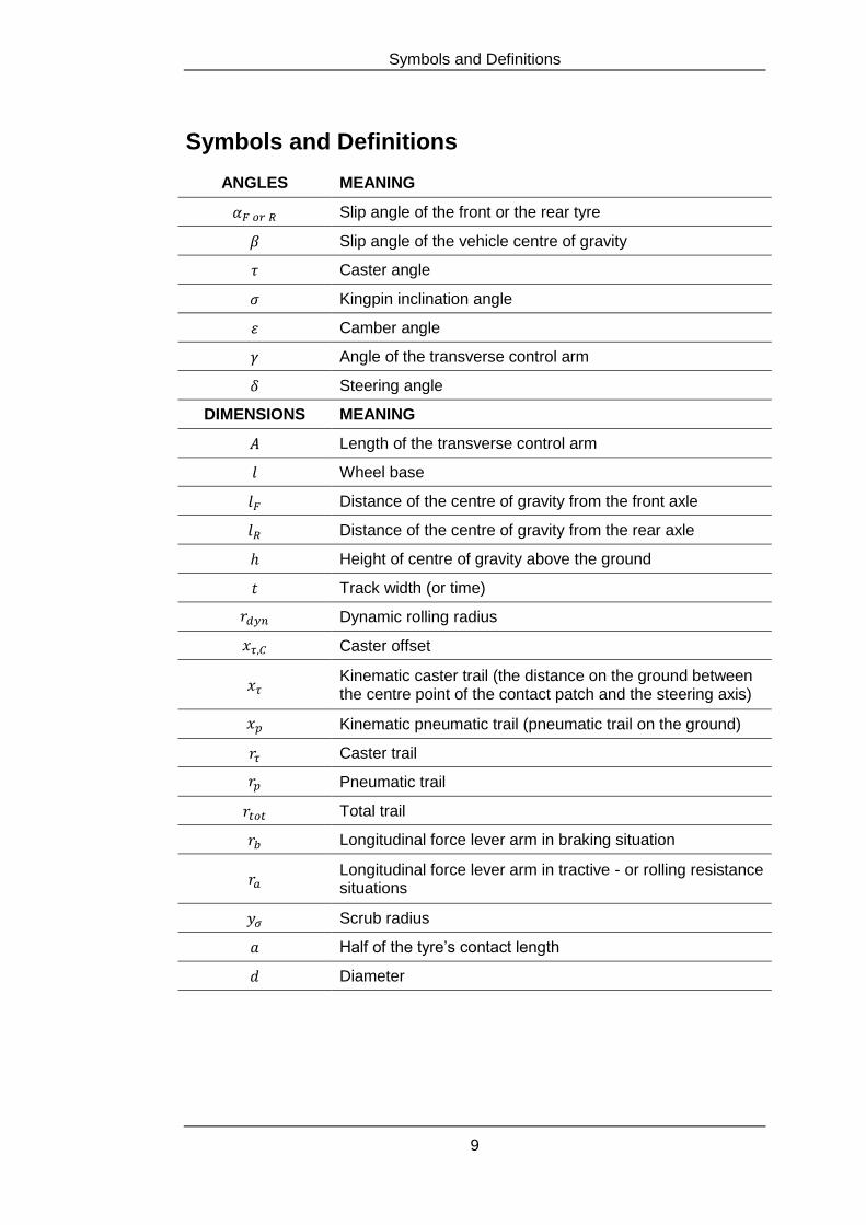
Symbols and Definitions
ANGLES MEANING
Slip angle of the front or the rear tyre
Slip angle of the vehicle centre of gravity
Caster angle
Kingpin inclination angle
Camber angle
Angle of the transverse control arm
Steering angle
DIMENSIONS MEANING
Length of the transverse control arm
Wheel base
Distance of the centre of gravity from the front axle
Distance of the centre of gravity from the rear axle
Height of centre of gravity above the ground
Track width (or time)
Dynamic rolling radius
Caster offset
Kinematic caster trail (the distance on the ground between the centre point of the contact patch and the steering axis)
Kinematic pneumatic trail (pneumatic trail on the ground)
Caster trail
Pneumatic trail
Total trail
Longitudinal force lever arm in braking situation
Longitudinal force lever arm in tractive - or rolling resistance situations
Scrub radius
Half of the tyre’s contact length
Diameter
Symbols and Definitions
10
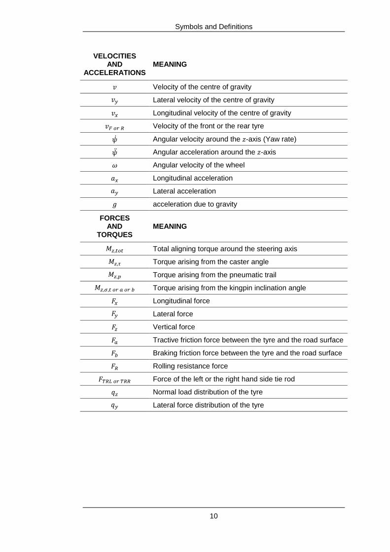
VELOCITIES AND
ACCELERATIONS MEANING
Velocity of the centre of gravity
Lateral velocity of the centre of gravity
Longitudinal velocity of the centre of gravity
Velocity of the front or the rear tyre
Angular velocity around the -axis (Yaw rate)
Angular acceleration around the -axis
Angular velocity of the wheel
Longitudinal acceleration
Lateral acceleration
acceleration due to gravity
FORCES AND
TORQUES MEANING
Total aligning torque around the steering axis
Torque arising from the caster angle
Torque arising from the pneumatic trail
Torque arising from the kingpin inclination angle
Longitudinal force
Lateral force
Vertical force
Tractive friction force between the tyre and the road surface
Braking friction force between the tyre and the road surface
Rolling resistance force
Force of the left or the right hand side tie rod
Normal load distribution of the tyre
Lateral force distribution of the tyre
Symbols and Definitions
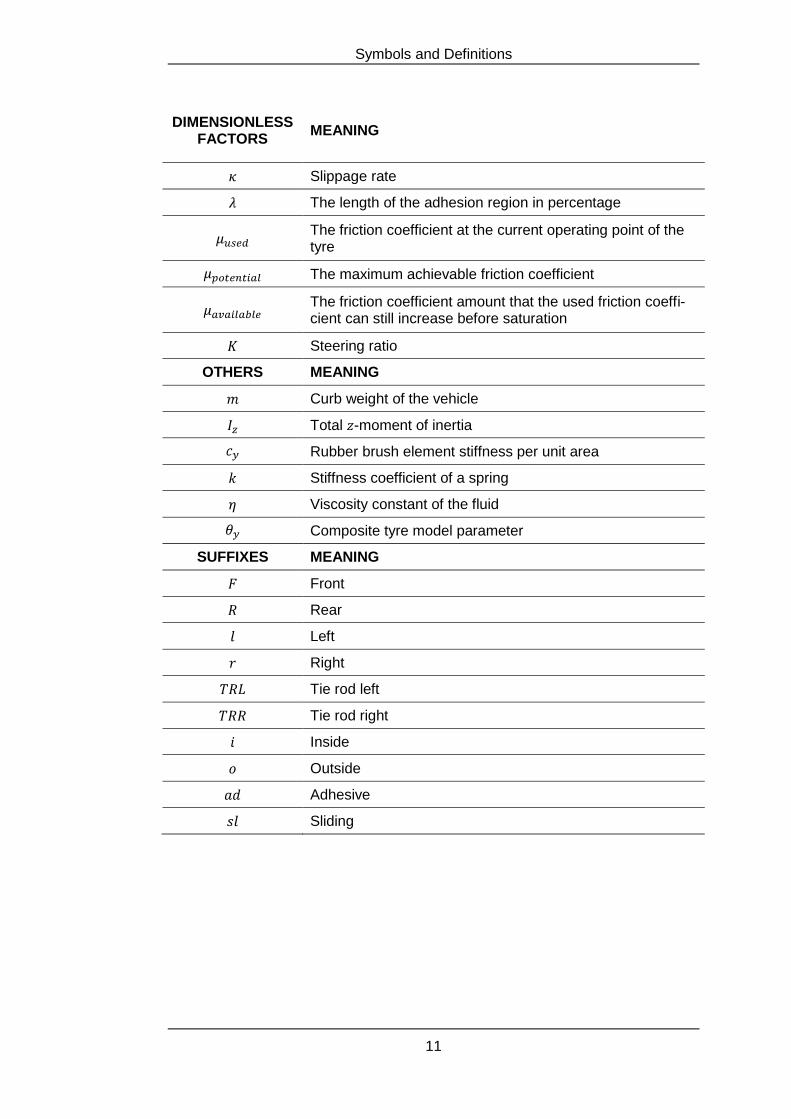
11
DIMENSIONLESS FACTORS
MEANING
Slippage rate
The length of the adhesion region in percentage
The friction coefficient at the current operating point of the tyre
The maximum achievable friction coefficient
The friction coefficient amount that the used friction coeffi-cient can still increase before saturation
Steering ratio
OTHERS MEANING
Curb weight of the vehicle
Total -moment of inertia
Rubber brush element stiffness per unit area
Stiffness coefficient of a spring
Viscosity constant of the fluid
Composite tyre model parameter
SUFFIXES MEANING
Front
Rear
Left
Right
Tie rod left
Tie rod right
Inside
Outside
Adhesive
Sliding
Abbreviations
12
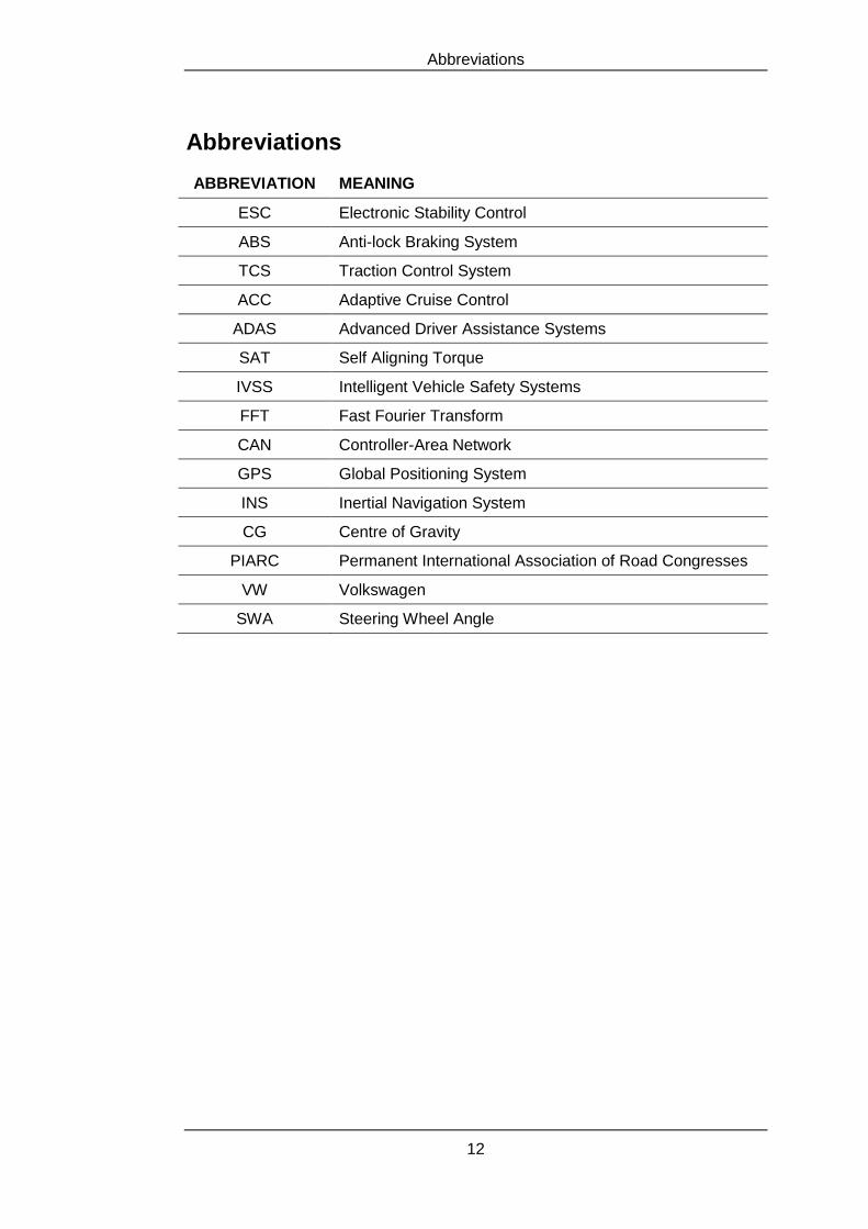
Abbreviations
ABBREVIATION MEANING
ESC Electronic Stability Control
ABS Anti-lock Braking System
TCS Traction Control System
ACC Adaptive Cruise Control
ADAS Advanced Driver Assistance Systems
SAT Self Aligning Torque
IVSS Intelligent Vehicle Safety Systems
FFT Fast Fourier Transform
CAN Controller-Area Network
GPS Global Positioning System
INS Inertial Navigation System
CG Centre of Gravity
PIARC Permanent International Association of Road Congresses
VW Volkswagen
SWA Steering Wheel Angle
Introduction
13
1 Introduction
1.1 Motivation and Background
The basic relationship between the driver and the vehicle has remained the same
from the early stages of automotive history. Still today the driver sits in the vehicle
and gives his/her desires to vehicle’s systems such as power transmission and
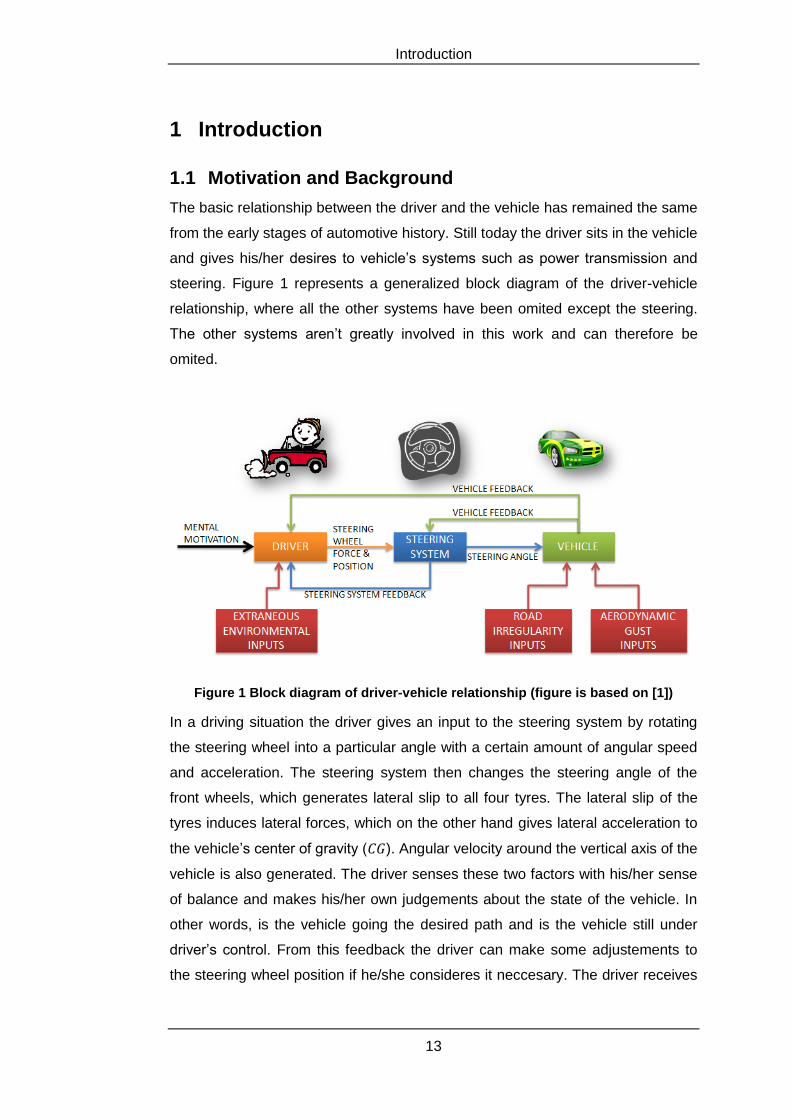
steering. Figure 1 represents a generalized block diagram of the driver-vehicle
relationship, where all the other systems have been omited except the steering.
The other systems aren’t greatly involved in this work and can therefore be
omited.
Figure 1 Block diagram of driver-vehicle relationship (figure is based on [1])
In a driving situation the driver gives an input to the steering system by rotating
the steering wheel into a particular angle with a certain amount of angular speed
and acceleration. The steering system then changes the steering angle of the
front wheels, which generates lateral slip to all four tyres. The lateral slip of the
tyres induces lateral forces, which on the other hand gives lateral acceleration to
the vehicle’s center of gravity ( ). Angular velocity around the vertical axis of the
vehicle is also generated. The driver senses these two factors with his/her sense
of balance and makes his/her own judgements about the state of the vehicle. In
other words, is the vehicle going the desired path and is the vehicle still under
driver’s control. From this feedback the driver can make some adjustements to
the steering wheel position if he/she consideres it neccesary. The driver receives
Introduction
14
another feedback from the steering system. The induced lateral forces at the
tyres don’t act at the steering axis, but a distance from it, which generates a
torque on both front tyres that attempts to return the wheels back in straight
ahead driving position. This torque is transmitted to the steering wheel via the
steering system and thus to the sense of feeling of the driver’s hands. Againg the
driver makes his/her own judgements about whether adjustments are required or
not. The driver gains also a lot of feedback via his/her sense of sight and hearing.
For example judgements of the road surface and its environmental conditions are
made by vision. Hearing on the other hand can be exploited for listening tyre
noises.
The only instruments that the driver has for evaluating the current state of the
vehicle are his/her own senses. Obviously the driver is placed under a challeging
task, since there comes a surge of information, which has to be evaluated imme-
diately. Fortunately modern vehicles are equipped with such active safety
systems as ESC, TCS, ABS and ACC. These systems utilize mostly the same
principles as the senses of the driver for gathering information about the state of
the vehicle. The difference is that these embedded system are more accurate
and consistent of making decisions than the driver. The senses and decisions
that the driver makes are always subjective and depend of many things such as
state of alertness and mental motivation. With the aid of these systems the
workload of the driver is relified and some of the mistakes that the driver makes
can be corrected. Altough the modern active safety systems work rather well,
they are lacking one major information, which is the knowledge of the tyre-road
friction potential. The maximum force that the tyre can generate is affected by the
friction potential of the specific tyre-road interface. Therefore the full performance
of the active safety systems and the upcoming advanced driver assistance
systems (ADAS) can be achieved only with the knowledge of friction potential.
The driver of course makes his/her own conclusions of the friction conditions
(Figure 2). Studies have nevertheless proved the drivers’ friction estimation ca-
pabilities being rather poor [2]. In addition the drivers’ conclusions can’t be
exploited to active safety systems. Therefore several different approaches for
estimating friction potential have been studied in research projects. These
different approaches are briefly discussed in Chapter 3.
Introduction
15
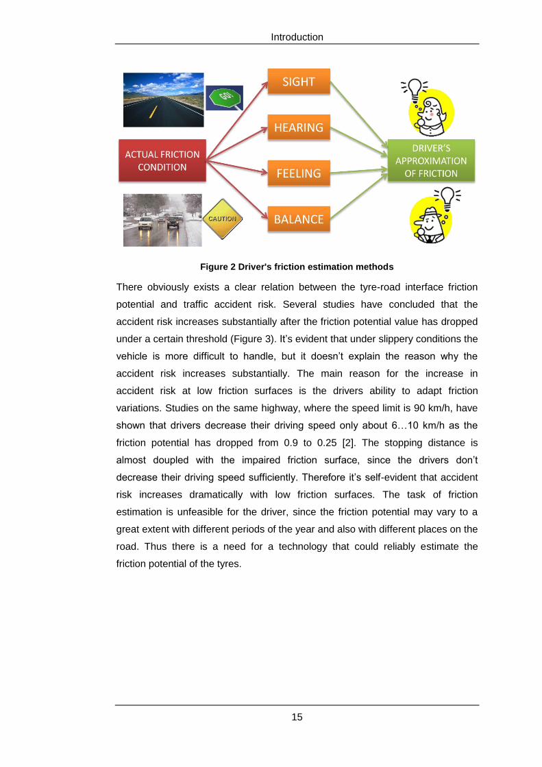
Figure 2 Driver's friction estimation methods
There obviously exists a clear relation between the tyre-road interface friction
potential and traffic accident risk. Several studies have concluded that the
accident risk increases substantially after the friction potential value has dropped
under a certain threshold (Figure 3). It’s evident that under slippery conditions the
vehicle is more difficult to handle, but it doesn’t explain the reason why the
accident risk increases substantially. The main reason for the increase in
accident risk at low friction surfaces is the drivers ability to adapt friction
variations. Studies on the same highway, where the speed limit is 90 km/h, have
shown that drivers decrease their driving speed only about 6…10 km/h as the
friction potential has dropped from 0.9 to 0.25 [2]. The stopping distance is
almost doupled with the impaired friction surface, since the drivers don’t
decrease their driving speed sufficiently. Therefore it’s self-evident that accident
risk increases dramatically with low friction surfaces. The task of friction
estimation is unfeasible for the driver, since the friction potential may vary to a
great extent with different periods of the year and also with different places on the
road. Thus there is a need for a technology that could reliably estimate the
friction potential of the tyres.
Introduction
16
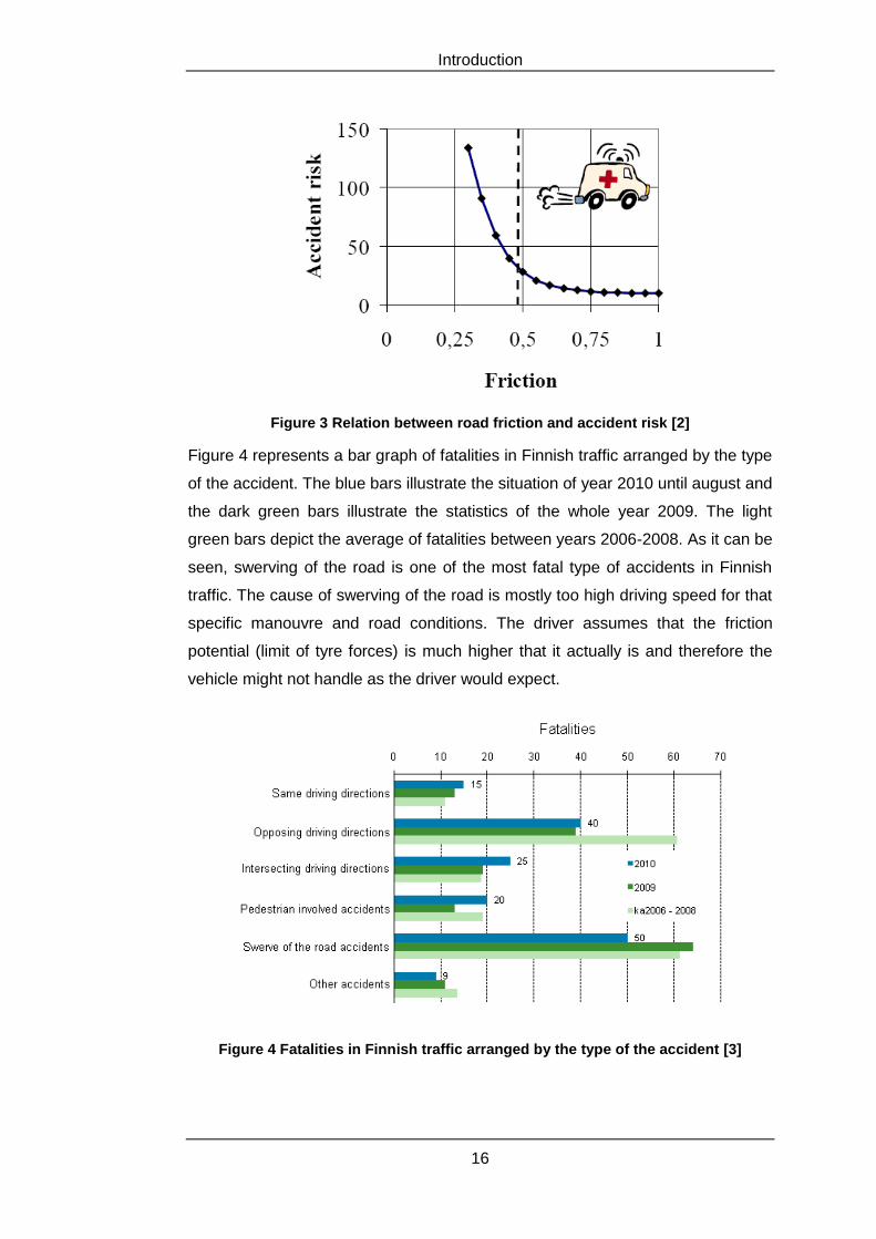
Figure 3 Relation between road friction and accident risk [2]
Figure 4 represents a bar graph of fatalities in Finnish traffic arranged by the type
of the accident. The blue bars illustrate the situation of year 2010 until august and
the dark green bars illustrate the statistics of the whole year 2009. The light
green bars depict the average of fatalities between years 2006-2008. As it can be
seen, swerving of the road is one of the most fatal type of accidents in Finnish
traffic. The cause of swerving of the road is mostly too high driving speed for that
specific manouvre and road conditions. The driver assumes that the friction
potential (limit of tyre forces) is much higher that it actually is and therefore the
vehicle might not handle as the driver would expect.
Figure 4 Fatalities in Finnish traffic arranged by the type of the accident [3]
Introduction
17
1.2 Problem Statement
All the forces that enable the vehicle to negotiate a bend or brake/accelerate are
generated in the tyre-road interface. Obviously the magnitude of the forces that
the tyre-road interface can produce has a limit. Beyond this limit, the whole con-
tact area of the tyre is sliding and therefore full control over the vehicle might be
lost. The maximum forces that the tyre-road interface can produce depends
mainly of the tyre - and road surface properties. The load - and the orientation of
the tyre relative to road surface have also a significant influence to the force limit.
The last two factors can be determined rather easily, but the detection of tyre-
road interface properties and conditions is much more challenging. In addition the
properties and conditions of the tyre-road interface may vary a lot in short term.
In order to get the full performance out of the active safety systems and ad-
vanced driver assistance systems, the maximum achievable forces of each tyre
should be known. For attaining this ambitious goal, the friction potential of each
tyre has to be evaluated in real-time. Several different approaches have been
studied over the years, which can be categorized into direct - and indirect meth-
ods. The categorization of estimation methods is discussed more detailed in
Chapter 3, but briefly, the direct methods are directly involved with the friction
process by measuring e.g. forces and accelerations of the vehicle or the tyre.
The indirect methods on the other hand are just related to the friction process in
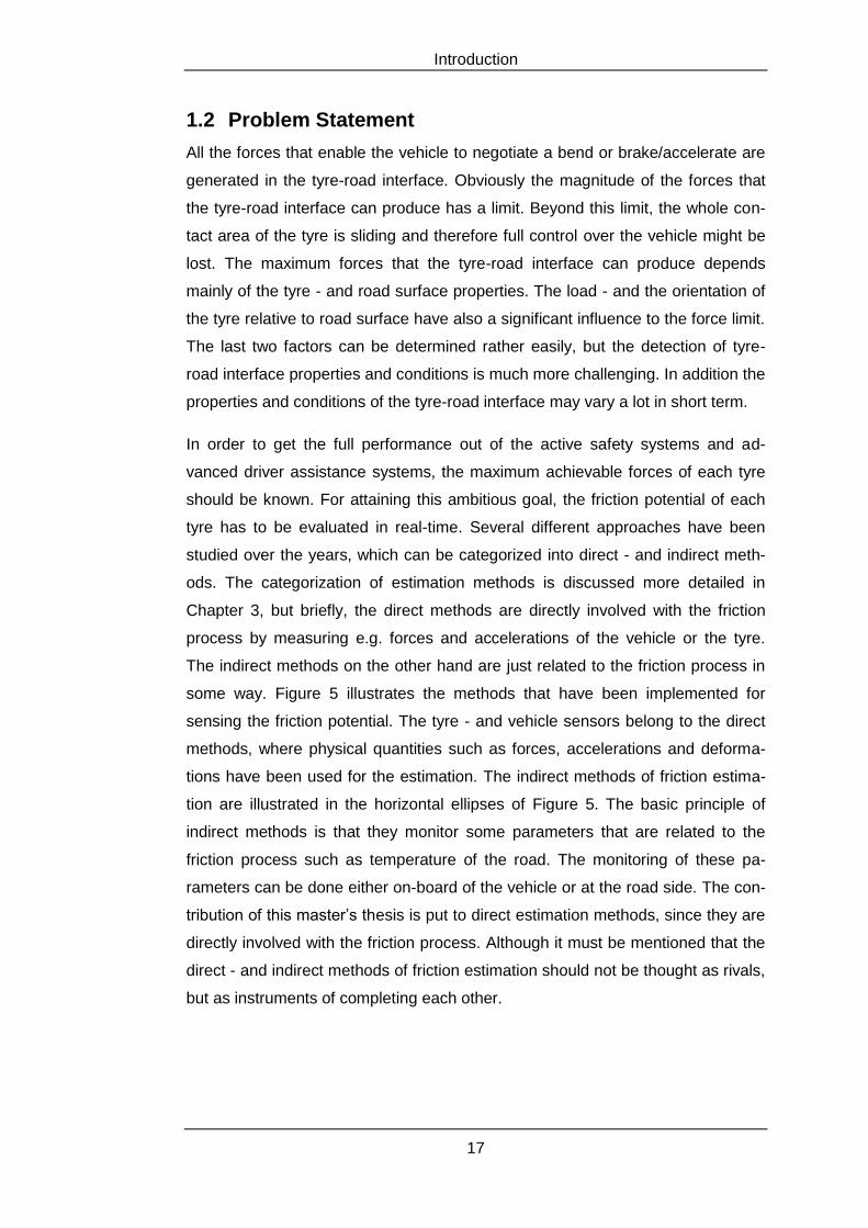
some way. Figure 5 illustrates the methods that have been implemented for
sensing the friction potential. The tyre - and vehicle sensors belong to the direct
methods, where physical quantities such as forces, accelerations and deforma-
tions have been used for the estimation. The indirect methods of friction estima-
tion are illustrated in the horizontal ellipses of Figure 5. The basic principle of
indirect methods is that they monitor some parameters that are related to the
friction process such as temperature of the road. The monitoring of these pa-
rameters can be done either on-board of the vehicle or at the road side. The con-
tribution of this master’s thesis is put to direct estimation methods, since they are
directly involved with the friction process. Although it must be mentioned that the
direct - and indirect methods of friction estimation should not be thought as rivals,
but as instruments of completing each other.
Introduction
18
Figure 5 Methods of sensing friction potential
The objective of this master’s thesis is to study the feasibility of estimating friction
potential by using the information of forces and torques that are generated in the
tyre-road interface. The Self Aligning Torque (SAT) that develops around the
wheel’s steering axis in a cornering manoeuvre is evaluated by measuring the
force of the tie rod. This torque is obviously induced by the lateral force, which
doesn’t act at the steering axis but at a distance from it. The planar motion of the
vehicle and thus the lateral forces of the front tyres are determined by exploiting
the famous bicycle model. Both the self aligning torque and the lateral force of
the tyre are given as inputs for the well-known brush tyre model, which ultimately
is used for the estimation of friction potential. The self aligning torque that is
evaluated from the tie rod force measurement can’t be given directly to the brush
tyre model, because it contains an additional torque, which arises from the
alignment of the steering axis. In order to subtract this additional torque from the
total self aligning torque, the lateral - and longitudinal inclination angles of the
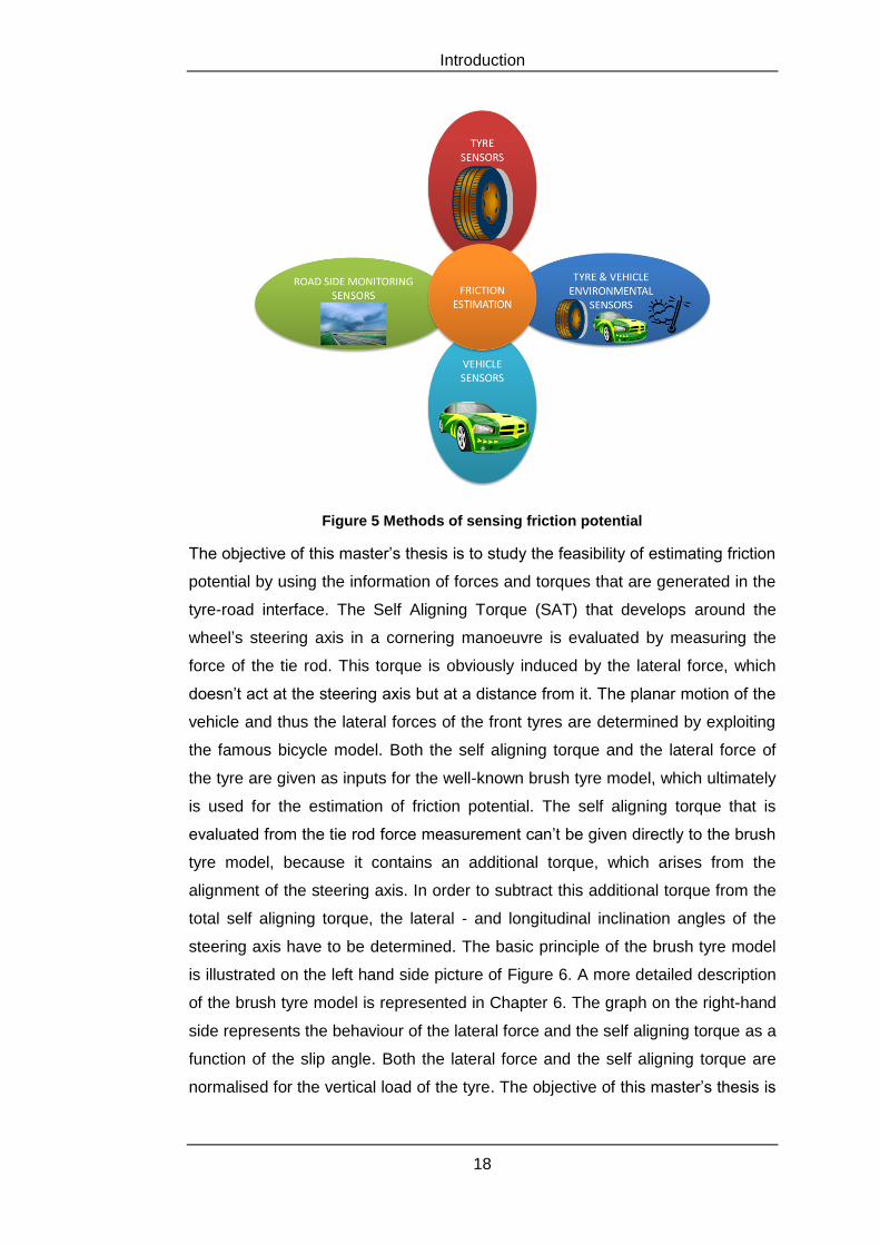
steering axis have to be determined. The basic principle of the brush tyre model
is illustrated on the left hand side picture of Figure 6. A more detailed description
of the brush tyre model is represented in Chapter 6. The graph on the right-hand
side represents the behaviour of the lateral force and the self aligning torque as a
function of the slip angle. Both the lateral force and the self aligning torque are
normalised for the vertical load of the tyre. The objective of this master’s thesis is
Introduction
19
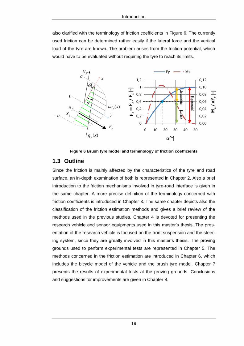
also clarified with the terminology of friction coefficients in Figure 6. The currently
used friction can be determined rather easily if the lateral force and the vertical
load of the tyre are known. The problem arises from the friction potential, which
would have to be evaluated without requiring the tyre to reach its limits.
a
yF
a txpx
0
Fv
x
)(xqz
)(xq y
y
Figure 6 Brush tyre model and terminology of friction coefficients
1.3 Outline
Since the friction is mainly affected by the characteristics of the tyre and road
surface, an in-depth examination of both is represented in Chapter 2. Also a brief
introduction to the friction mechanisms involved in tyre-road interface is given in
the same chapter. A more precise definition of the terminology concerned with
friction coefficients is introduced in Chapter 3. The same chapter depicts also the
classification of the friction estimation methods and gives a brief review of the
methods used in the previous studies. Chapter 4 is devoted for presenting the
research vehicle and sensor equipments used in this master’s thesis. The pres-
entation of the research vehicle is focused on the front suspension and the steer-
ing system, since they are greatly involved in this master’s thesis. The proving
grounds used to perform experimental tests are represented in Chapter 5. The
methods concerned in the friction estimation are introduced in Chapter 6, which
includes the bicycle model of the vehicle and the brush tyre model. Chapter 7
presents the results of experimental tests at the proving grounds. Conclusions
and suggestions for improvements are given in Chapter 8.
0,00
0,02
0,04
0,06
0,08
0,10
0,12
0
0,2
0,4
0,6
0,8
1
1,2
0 10 20 30 40 50
Mz
/ aF
y[-
]
µy
= F
y/
Fz
[-]
α[°]
Fy Mz
µavailab
le µ
used
µp
oten
tial
Introduction
20
1.4 Main Results
In this master’s thesis a typical small family estate car is used for proving ground
tests, where the feasibility of the estimation method is studied. Two distinguishing
proving grounds are chosen for illustrating the operation of the estimation method
on high - and low friction level surfaces. Tests also in -split conditions and in
situation where the vehicle is travelling from high friction level surface to low fric-
tion level surface are implemented. The friction estimation method considers only
a pure lateral slip situation and therefore all the test were performed with clutch
disengaged.
Results from the high friction level surface illustrate that the estimation method is
able to detect the friction states of the front tyres in steady state cornering ma-
noeuvres. The same tests at the low friction level surface provide also plausible
values of the front tyres friction state. Remarkable and interesting results are
found from the -split and surface transition tests were the estimation method is
able to distinguish the difference between the high- and low friction level sur-
faces.
The Rubber-Road Interface: Phenomena Involved in Friction
21
2 The Rubber-Road Interface: Phenomena Involved
in Friction
2.1 Introduction
Besides gravity and aerodynamic forces, the rubber-road interface is the place
where all the significant forces that act on a vehicle are generated. The area of
contact between these components is around the size of an average mans palm.
An in-depth examination of the interface components (rubber and road) and the
friction mechanisms involved in the contact are essential for understanding how
the vehicle is able to manoeuvre relying only to these relatively small contact
patches.
2.2 Characteristics of Rubber
2.2.1 Visco-elastic Behaviour
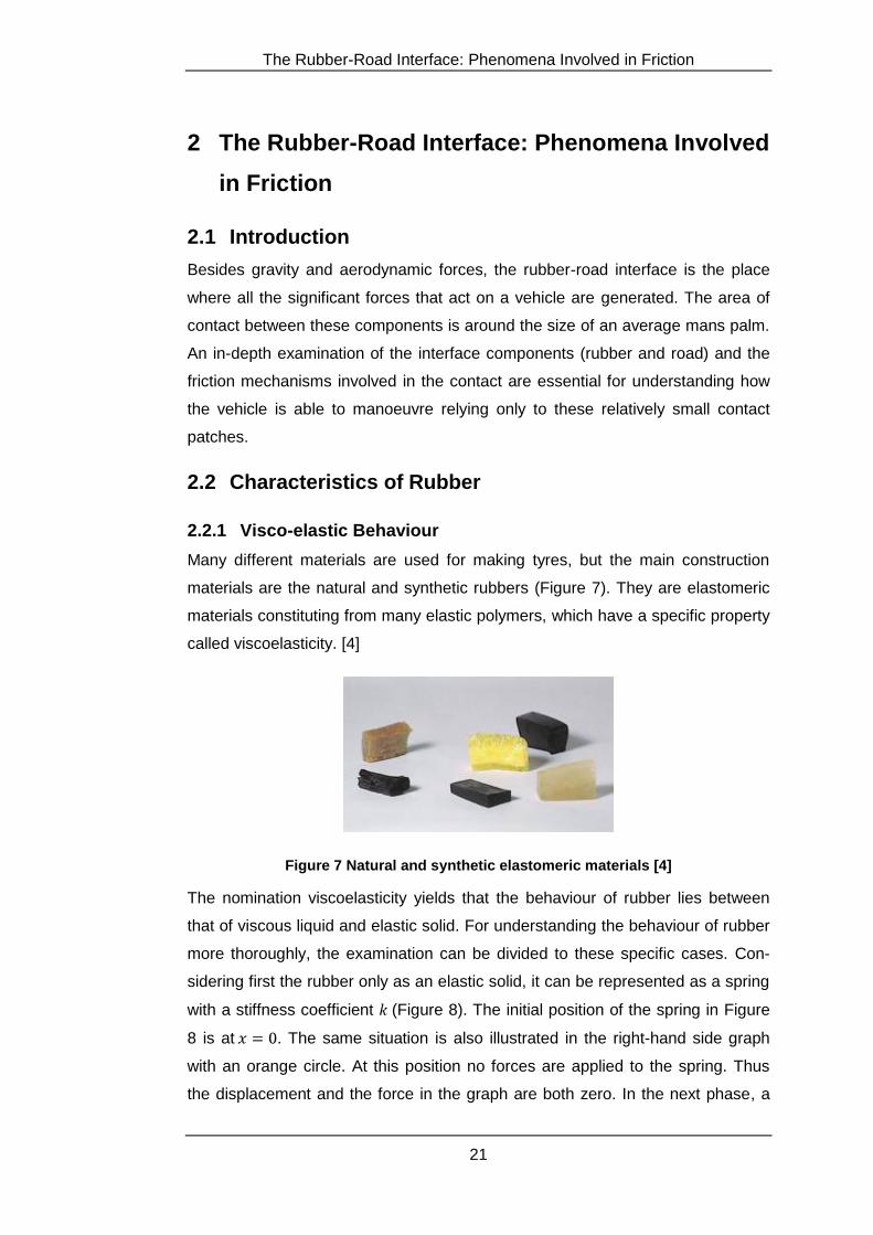
Many different materials are used for making tyres, but the main construction
materials are the natural and synthetic rubbers (Figure 7). They are elastomeric
materials constituting from many elastic polymers, which have a specific property
called viscoelasticity. [4]
Figure 7 Natural and synthetic elastomeric materials [4]
The nomination viscoelasticity yields that the behaviour of rubber lies between
that of viscous liquid and elastic solid. For understanding the behaviour of rubber
more thoroughly, the examination can be divided to these specific cases. Con-
sidering first the rubber only as an elastic solid, it can be represented as a spring
with a stiffness coefficient (Figure 8). The initial position of the spring in Figure
8 is at . The same situation is also illustrated in the right-hand side graph
with an orange circle. At this position no forces are applied to the spring. Thus
the displacement and the force in the graph are both zero. In the next phase, a
The Rubber-Road Interface: Phenomena Involved in Friction
22
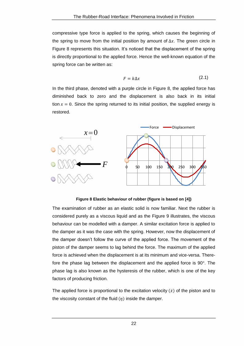
compressive type force is applied to the spring, which causes the beginning of
the spring to move from the initial position by amount of . The green circle in
Figure 8 represents this situation. It’s noticed that the displacement of the spring
is directly proportional to the applied force. Hence the well-known equation of the
spring force can be written as:
(2.1)
In the third phase, denoted with a purple circle in Figure 8, the applied force has
diminished back to zero and the displacement is also back in its initial
tion . Since the spring returned to its initial position, the supplied energy is
restored.
F
0x
Figure 8 Elastic behaviour of rubber (figure is based on [4])
The examination of rubber as an elastic solid is now familiar. Next the rubber is
considered purely as a viscous liquid and as the Figure 9 illustrates, the viscous
behaviour can be modelled with a damper. A similar excitation force is applied to
the damper as it was the case with the spring. However, now the displacement of
the damper doesn’t follow the curve of the applied force. The movement of the
piston of the damper seems to lag behind the force. The maximum of the applied
force is achieved when the displacement is at its minimum and vice-versa. There-
fore the phase lag between the displacement and the applied force is 90 . The
phase lag is also known as the hysteresis of the rubber, which is one of the key
factors of producing friction.
The applied force is proportional to the excitation velocity of the piston and to
the viscosity constant of the fluid inside the damper.
0 50 100 150 200 250 300 350
Force Displacement
The Rubber-Road Interface: Phenomena Involved in Friction
23
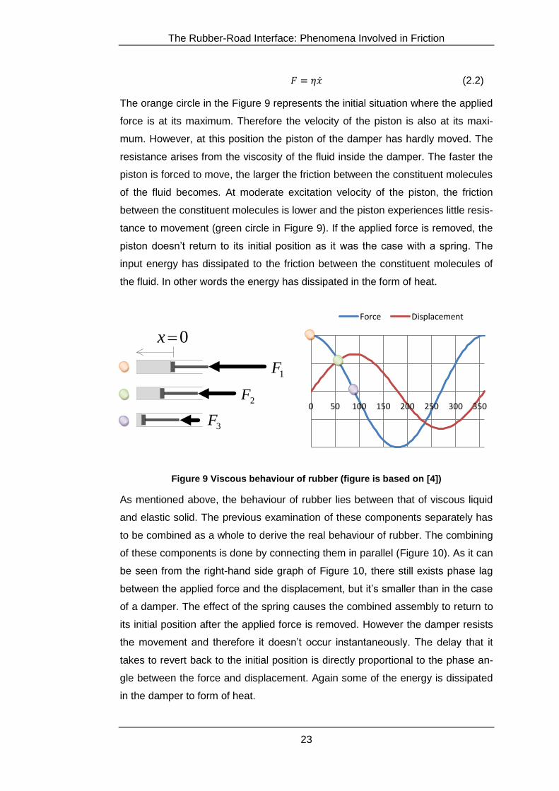
(2.2)
The orange circle in the Figure 9 represents the initial situation where the applied
force is at its maximum. Therefore the velocity of the piston is also at its maxi-
mum. However, at this position the piston of the damper has hardly moved. The
resistance arises from the viscosity of the fluid inside the damper. The faster the
piston is forced to move, the larger the friction between the constituent molecules
of the fluid becomes. At moderate excitation velocity of the piston, the friction
between the constituent molecules is lower and the piston experiences little resis-
tance to movement (green circle in Figure 9). If the applied force is removed, the
piston doesn’t return to its initial position as it was the case with a spring. The
input energy has dissipated to the friction between the constituent molecules of
the fluid. In other words the energy has dissipated in the form of heat.
0x
1F
2F
3F
Figure 9 Viscous behaviour of rubber (figure is based on [4])
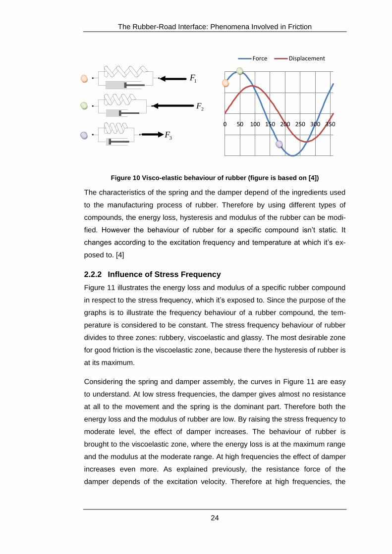
As mentioned above, the behaviour of rubber lies between that of viscous liquid
and elastic solid. The previous examination of these components separately has
to be combined as a whole to derive the real behaviour of rubber. The combining
of these components is done by connecting them in parallel (Figure 10). As it can
be seen from the right-hand side graph of Figure 10, there still exists phase lag
between the applied force and the displacement, but it’s smaller than in the case
of a damper. The effect of the spring causes the combined assembly to return to
its initial position after the applied force is removed. However the damper resists
the movement and therefore it doesn’t occur instantaneously. The delay that it
takes to revert back to the initial position is directly proportional to the phase an-
gle between the force and displacement. Again some of the energy is dissipated
in the damper to form of heat.
0 50 100 150 200 250 300 350
Force Displacement
The Rubber-Road Interface: Phenomena Involved in Friction
24
1F
2F
3F
Figure 10 Visco-elastic behaviour of rubber (figure is based on [4])
The characteristics of the spring and the damper depend of the ingredients used
to the manufacturing process of rubber. Therefore by using different types of
compounds, the energy loss, hysteresis and modulus of the rubber can be modi-
fied. However the behaviour of rubber for a specific compound isn’t static. It
changes according to the excitation frequency and temperature at which it’s ex-
posed to. [4]
2.2.2 Influence of Stress Frequency
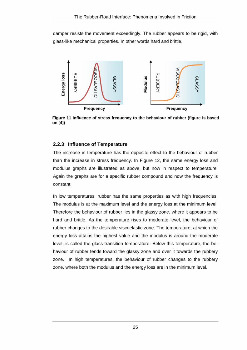
Figure 11 illustrates the energy loss and modulus of a specific rubber compound
in respect to the stress frequency, which it’s exposed to. Since the purpose of the
graphs is to illustrate the frequency behaviour of a rubber compound, the tem-
perature is considered to be constant. The stress frequency behaviour of rubber
divides to three zones: rubbery, viscoelastic and glassy. The most desirable zone
for good friction is the viscoelastic zone, because there the hysteresis of rubber is
at its maximum.
Considering the spring and damper assembly, the curves in Figure 11 are easy
to understand. At low stress frequencies, the damper gives almost no resistance
at all to the movement and the spring is the dominant part. Therefore both the
energy loss and the modulus of rubber are low. By raising the stress frequency to
moderate level, the effect of damper increases. The behaviour of rubber is
brought to the viscoelastic zone, where the energy loss is at the maximum range
and the modulus at the moderate range. At high frequencies the effect of damper
increases even more. As explained previously, the resistance force of the
damper depends of the excitation velocity. Therefore at high frequencies, the
0 50 100 150 200 250 300 350
Force Displacement
The Rubber-Road Interface: Phenomena Involved in Friction
25
damper resists the movement exceedingly. The rubber appears to be rigid, with
glass-like mechanical properties. In other words hard and brittle.
2.2.3 Influence of Temperature
The increase in temperature has the opposite effect to the behaviour of rubber
than the increase in stress frequency. In Figure 12, the same energy loss and
modulus graphs are illustrated as above, but now in respect to temperature.
Again the graphs are for a specific rubber compound and now the frequency is
constant.
In low temperatures, rubber has the same properties as with high frequencies.
The modulus is at the maximum level and the energy loss at the minimum level.
Therefore the behaviour of rubber lies in the glassy zone, where it appears to be
hard and brittle. As the temperature rises to moderate level, the behaviour of
rubber changes to the desirable viscoelastic zone. The temperature, at which the
energy loss attains the highest value and the modulus is around the moderate
level, is called the glass transition temperature. Below this temperature, the be-
haviour of rubber tends toward the glassy zone and over it towards the rubbery
zone. In high temperatures, the behaviour of rubber changes to the rubbery
zone, where both the modulus and the energy loss are in the minimum level.
Frequency
RU
BB
ER
Y
GLA
SS
Y M
od
ulu
s
VIS
CO
EL
AS
TIC
Frequency
VIS
CO
EL
AS
TIC
RU
BB
ER
Y
GLA
SS
Y
En
erg
y lo
ss
Figure 11 Influence of stress frequency to the behaviour of rubber (figure is based on [4])
The Rubber-Road Interface: Phenomena Involved in Friction
26
2.3 Characteristics of Road Surfaces
2.3.1 Texture
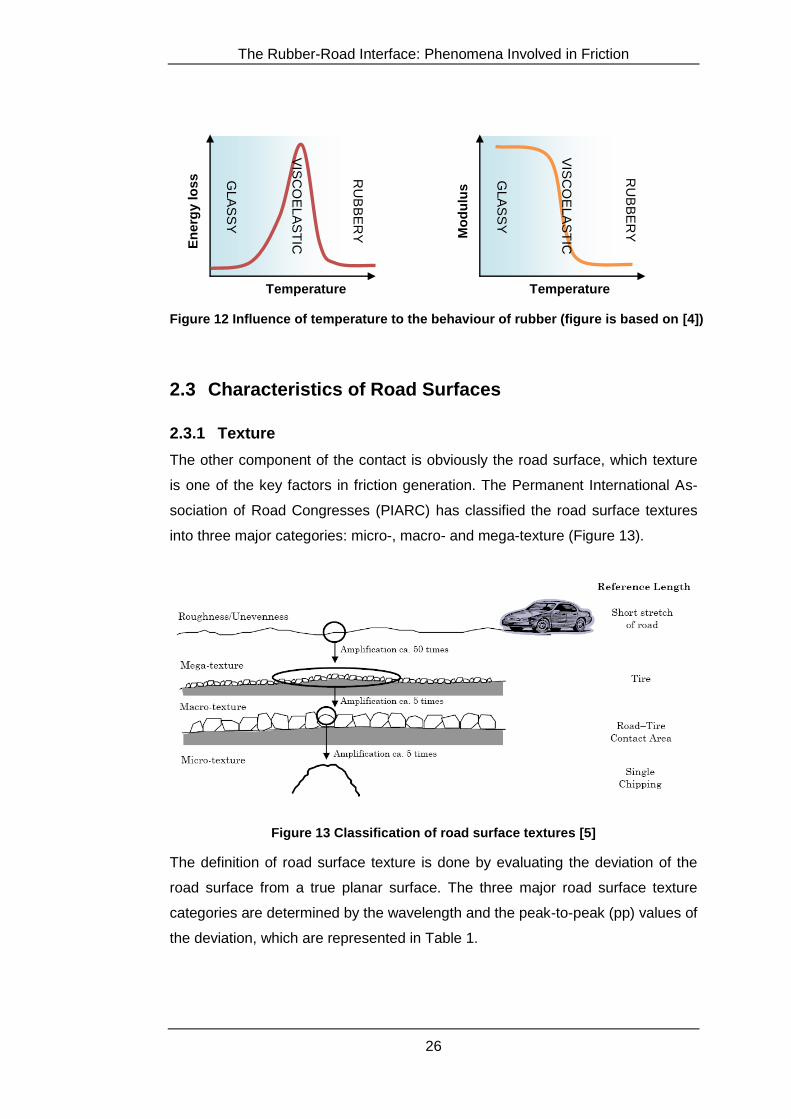
The other component of the contact is obviously the road surface, which texture
is one of the key factors in friction generation. The Permanent International As-
sociation of Road Congresses (PIARC) has classified the road surface textures
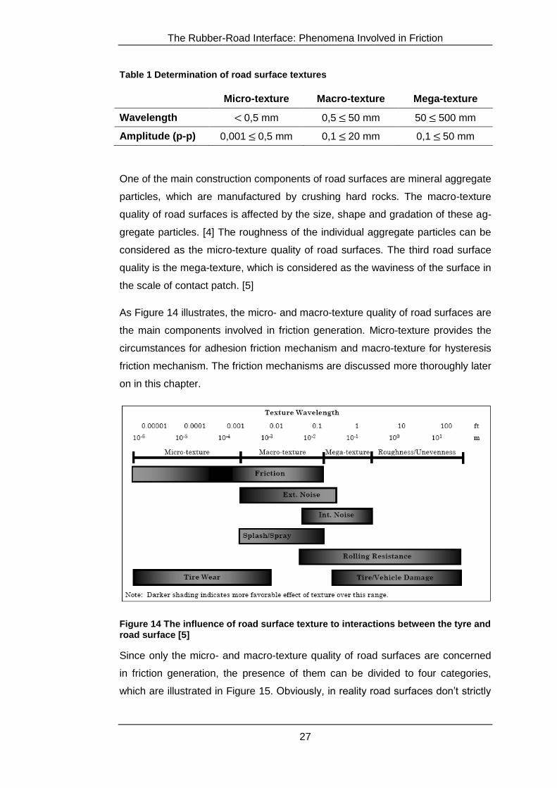
into three major categories: micro-, macro- and mega-texture (Figure 13).
Figure 13 Classification of road surface textures [5]
The definition of road surface texture is done by evaluating the deviation of the
road surface from a true planar surface. The three major road surface texture
categories are determined by the wavelength and the peak-to-peak (pp) values of
the deviation, which are represented in Table 1.
Temperature
RU
BB
ER
Y
GLA
SS
Y M
od
ulu
s
VIS
CO
EL
AS
TIC
Temperature
VIS
CO
EL
AS
TIC
RU
BB
ER
Y
GLA
SS
Y
En
erg
y lo
ss
Figure 12 Influence of temperature to the behaviour of rubber (figure is based on [4])
The Rubber-Road Interface: Phenomena Involved in Friction
27
Table 1 Determination of road surface textures
Micro-texture Macro-texture Mega-texture
Wavelength 0,5 mm 0,5 50 mm 50 500 mm
Amplitude (p-p) 0,001 0,5 mm 0,1 20 mm 0,1 50 mm
One of the main construction components of road surfaces are mineral aggregate
particles, which are manufactured by crushing hard rocks. The macro-texture
quality of road surfaces is affected by the size, shape and gradation of these ag-
gregate particles. [4] The roughness of the individual aggregate particles can be
considered as the micro-texture quality of road surfaces. The third road surface
quality is the mega-texture, which is considered as the waviness of the surface in
the scale of contact patch. [5]
As Figure 14 illustrates, the micro- and macro-texture quality of road surfaces are
the main components involved in friction generation. Micro-texture provides the
circumstances for adhesion friction mechanism and macro-texture for hysteresis
friction mechanism. The friction mechanisms are discussed more thoroughly later
on in this chapter.
Figure 14 The influence of road surface texture to interactions between the tyre and road surface [5]
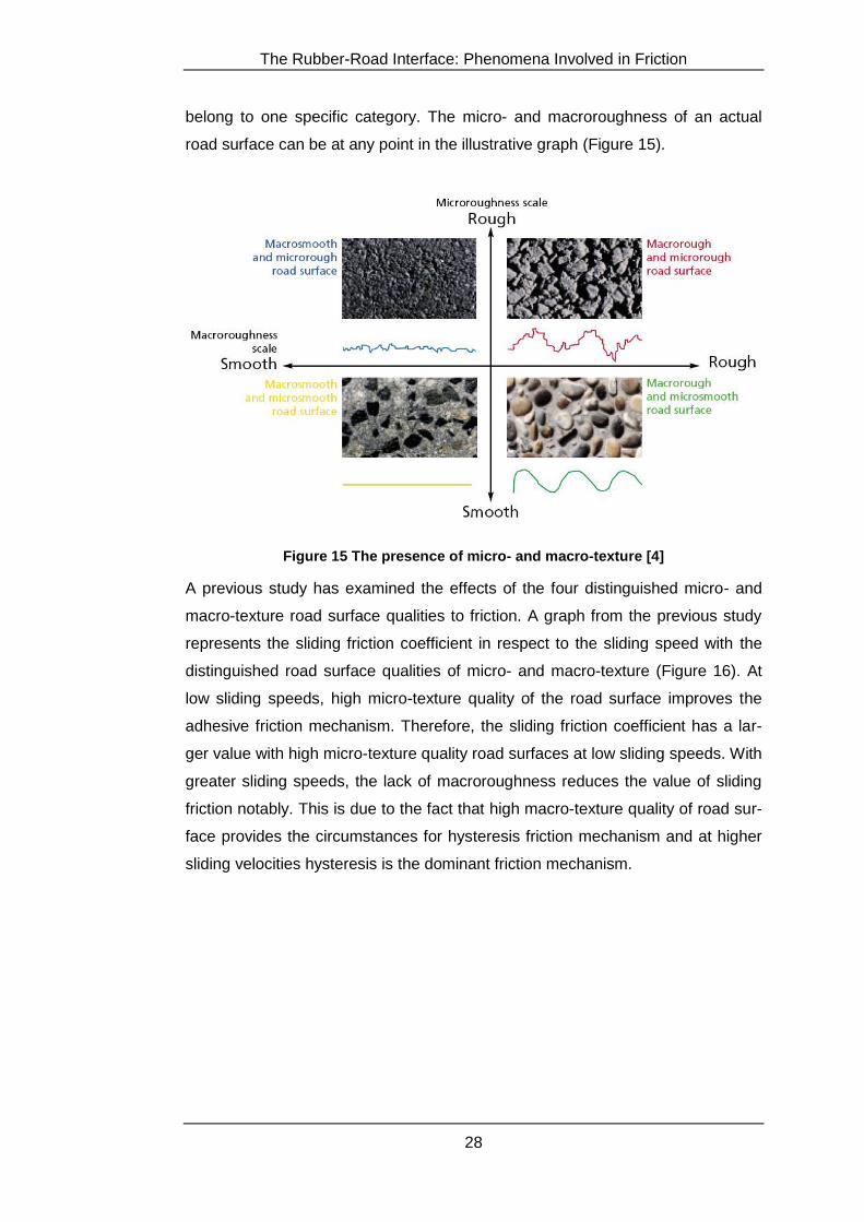
Since only the micro- and macro-texture quality of road surfaces are concerned
in friction generation, the presence of them can be divided to four categories,
which are illustrated in Figure 15. Obviously, in reality road surfaces don’t strictly
The Rubber-Road Interface: Phenomena Involved in Friction
28
belong to one specific category. The micro- and macroroughness of an actual
road surface can be at any point in the illustrative graph (Figure 15).
Figure 15 The presence of micro- and macro-texture [4]
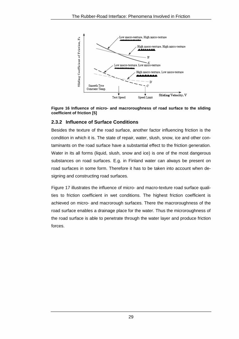
A previous study has examined the effects of the four distinguished micro- and
macro-texture road surface qualities to friction. A graph from the previous study
represents the sliding friction coefficient in respect to the sliding speed with the
distinguished road surface qualities of micro- and macro-texture (Figure 16). At
low sliding speeds, high micro-texture quality of the road surface improves the
adhesive friction mechanism. Therefore, the sliding friction coefficient has a lar-
ger value with high micro-texture quality road surfaces at low sliding speeds. With
greater sliding speeds, the lack of macroroughness reduces the value of sliding
friction notably. This is due to the fact that high macro-texture quality of road sur-
face provides the circumstances for hysteresis friction mechanism and at higher
sliding velocities hysteresis is the dominant friction mechanism.
The Rubber-Road Interface: Phenomena Involved in Friction
29
Figure 16 Influence of micro- and macroroughness of road surface to the sliding coefficient of friction [5]
2.3.2 Influence of Surface Conditions
Besides the texture of the road surface, another factor influencing friction is the
condition in which it is. The state of repair, water, slush, snow, ice and other con-
taminants on the road surface have a substantial effect to the friction generation.
Water in its all forms (liquid, slush, snow and ice) is one of the most dangerous
substances on road surfaces. E.g. in Finland water can always be present on
road surfaces in some form. Therefore it has to be taken into account when de-
signing and constructing road surfaces.
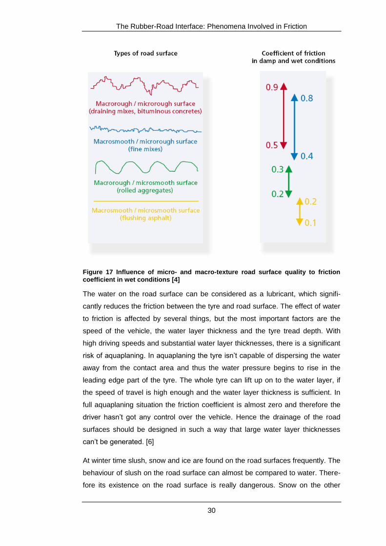
Figure 17 illustrates the influence of micro- and macro-texture road surface quali-
ties to friction coefficient in wet conditions. The highest friction coefficient is
achieved on micro- and macrorough surfaces. There the macroroughness of the
road surface enables a drainage place for the water. Thus the microroughness of
the road surface is able to penetrate through the water layer and produce friction
forces.
The Rubber-Road Interface: Phenomena Involved in Friction
30
Figure 17 Influence of micro- and macro-texture road surface quality to friction coefficient in wet conditions [4]
The water on the road surface can be considered as a lubricant, which signifi-
cantly reduces the friction between the tyre and road surface. The effect of water
to friction is affected by several things, but the most important factors are the
speed of the vehicle, the water layer thickness and the tyre tread depth. With
high driving speeds and substantial water layer thicknesses, there is a significant
risk of aquaplaning. In aquaplaning the tyre isn’t capable of dispersing the water
away from the contact area and thus the water pressure begins to rise in the
leading edge part of the tyre. The whole tyre can lift up on to the water layer, if
the speed of travel is high enough and the water layer thickness is sufficient. In
full aquaplaning situation the friction coefficient is almost zero and therefore the
driver hasn’t got any control over the vehicle. Hence the drainage of the road
surfaces should be designed in such a way that large water layer thicknesses
can’t be generated. [6]
At winter time slush, snow and ice are found on the road surfaces frequently. The
behaviour of slush on the road surface can almost be compared to water. There-
fore its existence on the road surface is really dangerous. Snow on the other
The Rubber-Road Interface: Phenomena Involved in Friction
31
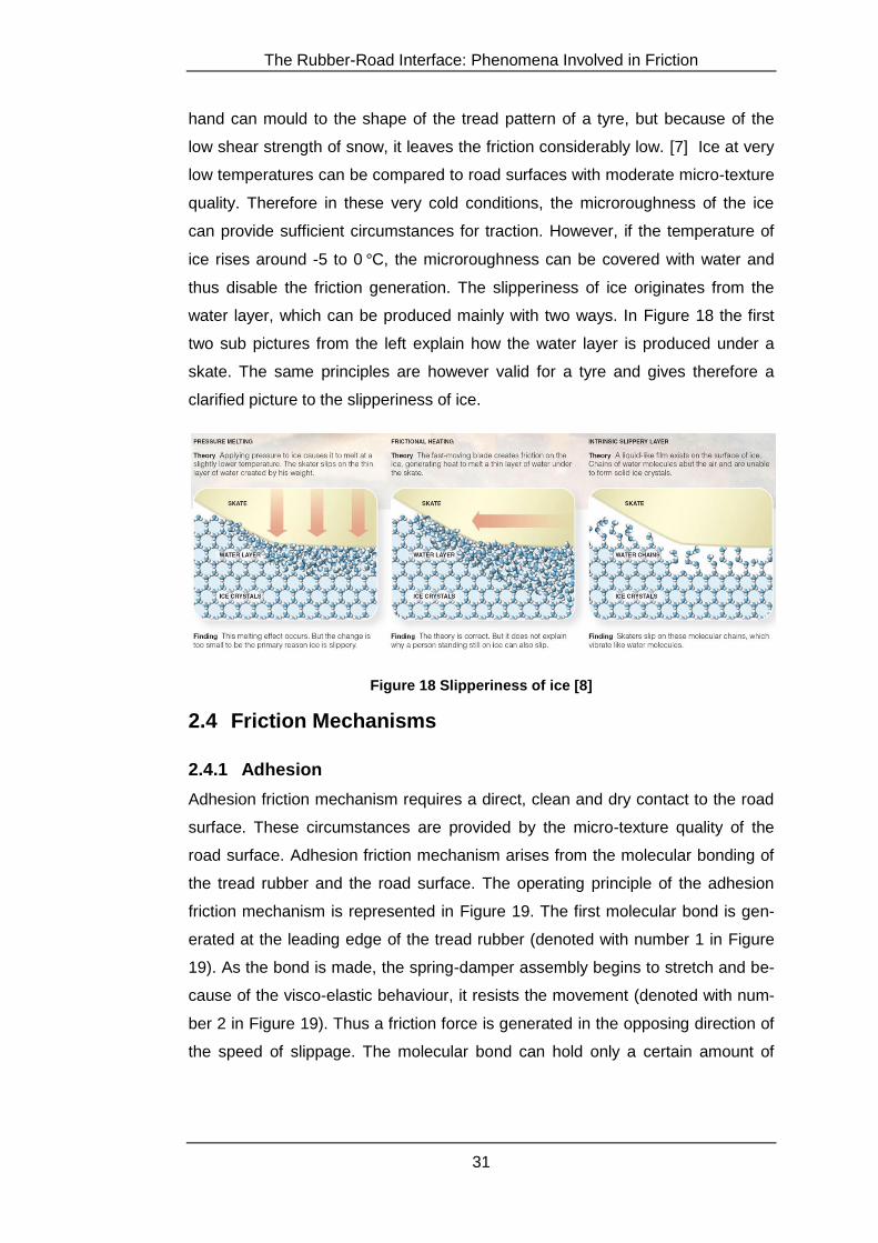
hand can mould to the shape of the tread pattern of a tyre, but because of the
low shear strength of snow, it leaves the friction considerably low. [7] Ice at very
low temperatures can be compared to road surfaces with moderate micro-texture
quality. Therefore in these very cold conditions, the microroughness of the ice
can provide sufficient circumstances for traction. However, if the temperature of
ice rises around -5 to 0 C, the microroughness can be covered with water and
thus disable the friction generation. The slipperiness of ice originates from the
water layer, which can be produced mainly with two ways. In Figure 18 the first
two sub pictures from the left explain how the water layer is produced under a
skate. The same principles are however valid for a tyre and gives therefore a
clarified picture to the slipperiness of ice.
Figure 18 Slipperiness of ice [8]
2.4 Friction Mechanisms
2.4.1 Adhesion
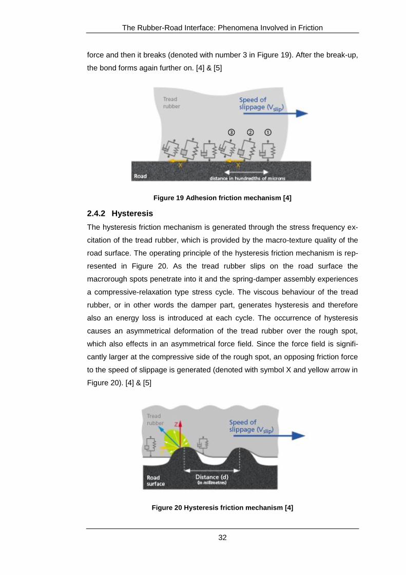
Adhesion friction mechanism requires a direct, clean and dry contact to the road
surface. These circumstances are provided by the micro-texture quality of the
road surface. Adhesion friction mechanism arises from the molecular bonding of
the tread rubber and the road surface. The operating principle of the adhesion
friction mechanism is represented in Figure 19. The first molecular bond is gen-
erated at the leading edge of the tread rubber (denoted with number 1 in Figure
19). As the bond is made, the spring-damper assembly begins to stretch and be-
cause of the visco-elastic behaviour, it resists the movement (denoted with num-
ber 2 in Figure 19). Thus a friction force is generated in the opposing direction of
the speed of slippage. The molecular bond can hold only a certain amount of
The Rubber-Road Interface: Phenomena Involved in Friction
32
force and then it breaks (denoted with number 3 in Figure 19). After the break-up,
the bond forms again further on. [4] & [5]
Figure 19 Adhesion friction mechanism [4]
2.4.2 Hysteresis
The hysteresis friction mechanism is generated through the stress frequency ex-
citation of the tread rubber, which is provided by the macro-texture quality of the
road surface. The operating principle of the hysteresis friction mechanism is rep-
resented in Figure 20. As the tread rubber slips on the road surface the
macrorough spots penetrate into it and the spring-damper assembly experiences
a compressive-relaxation type stress cycle. The viscous behaviour of the tread
rubber, or in other words the damper part, generates hysteresis and therefore
also an energy loss is introduced at each cycle. The occurrence of hysteresis
causes an asymmetrical deformation of the tread rubber over the rough spot,
which also effects in an asymmetrical force field. Since the force field is signifi-
cantly larger at the compressive side of the rough spot, an opposing friction force
to the speed of slippage is generated (denoted with symbol X and yellow arrow in
Figure 20). [4] & [5]
Figure 20 Hysteresis friction mechanism [4]
The Rubber-Road Interface: Phenomena Involved in Friction
33
2.5 Conclusions of this Chapter
The examination of the rubber and road surfaces properties illustrated that both
of them have a significant influence to the friction generation process. Also the
excess medium, such as water, between the tyre and road surface plays a major
role on the attainable friction. Several essential issues have to be taken into ac-
count when designing tread rubbers for tyres and surfaces for roads. These in-
clude such issues as the temperature at which the tread rubber compound is de-
signed to operate (summer - or winter tyre). In the road surface design process
the most important issue is to consider the effect of water. The surface texture
should have high microroughness to ensure traction in wet conditions and the
drainage of water should be designed in a way that no high water layers are gen-
erated.
Background and Theory of Friction Estimation
34
3 Background and Theory of Friction Estimation
3.1 Introduction
The attainable traction between the tyre and the road surface depends always of
the specific rubber-road interface properties and the conditions that they are ex-
posed to. It’s obvious that there are several different types of road surfaces,
which state of repair and surface conditions vary a lot between each other. Each
vehicle on the roads has their own specific set of tyres, which conditions vary
also from vehicle to vehicle. Since the circumstances for traction are so variable,
it would be essential to evaluate the current traction conditions in real-time.
There have been several studies concerning friction estimation of rubber-road
interface with various different methods. The purpose of this chapter is to give an
insight to the theory and methods that has been discovered during these previ-
ous studies.
3.2 Friction Coefficient
3.2.1 Definition
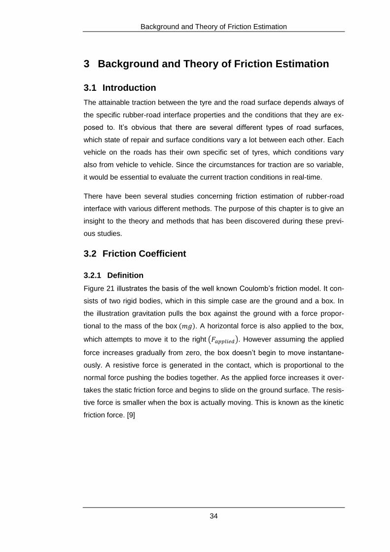
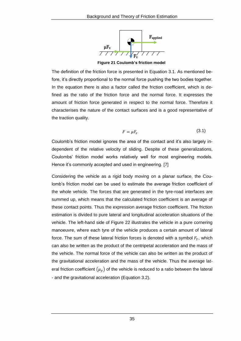
Figure 21 illustrates the basis of the well known Coulomb’s friction model. It con-
sists of two rigid bodies, which in this simple case are the ground and a box. In
the illustration gravitation pulls the box against the ground with a force propor-
tional to the mass of the box . A horizontal force is also applied to the box,
which attempts to move it to the right . However assuming the applied
force increases gradually from zero, the box doesn’t begin to move instantane-
ously. A resistive force is generated in the contact, which is proportional to the
normal force pushing the bodies together. As the applied force increases it over-
takes the static friction force and begins to slide on the ground surface. The resis-
tive force is smaller when the box is actually moving. This is known as the kinetic
friction force. [9]
Background and Theory of Friction Estimation
35
The definition of the friction force is presented in Equation 3.1. As mentioned be-
fore, it’s directly proportional to the normal force pushing the two bodies together.
In the equation there is also a factor called the friction coefficient, which is de-
fined as the ratio of the friction force and the normal force. It expresses the
amount of friction force generated in respect to the normal force. Therefore it
characterises the nature of the contact surfaces and is a good representative of
the traction quality.
(3.1)
Coulomb’s friction model ignores the area of the contact and it’s also largely in-
dependent of the relative velocity of sliding. Despite of these generalizations,
Coulombs’ friction model works relatively well for most engineering models.
Hence it’s commonly accepted and used in engineering. [7]
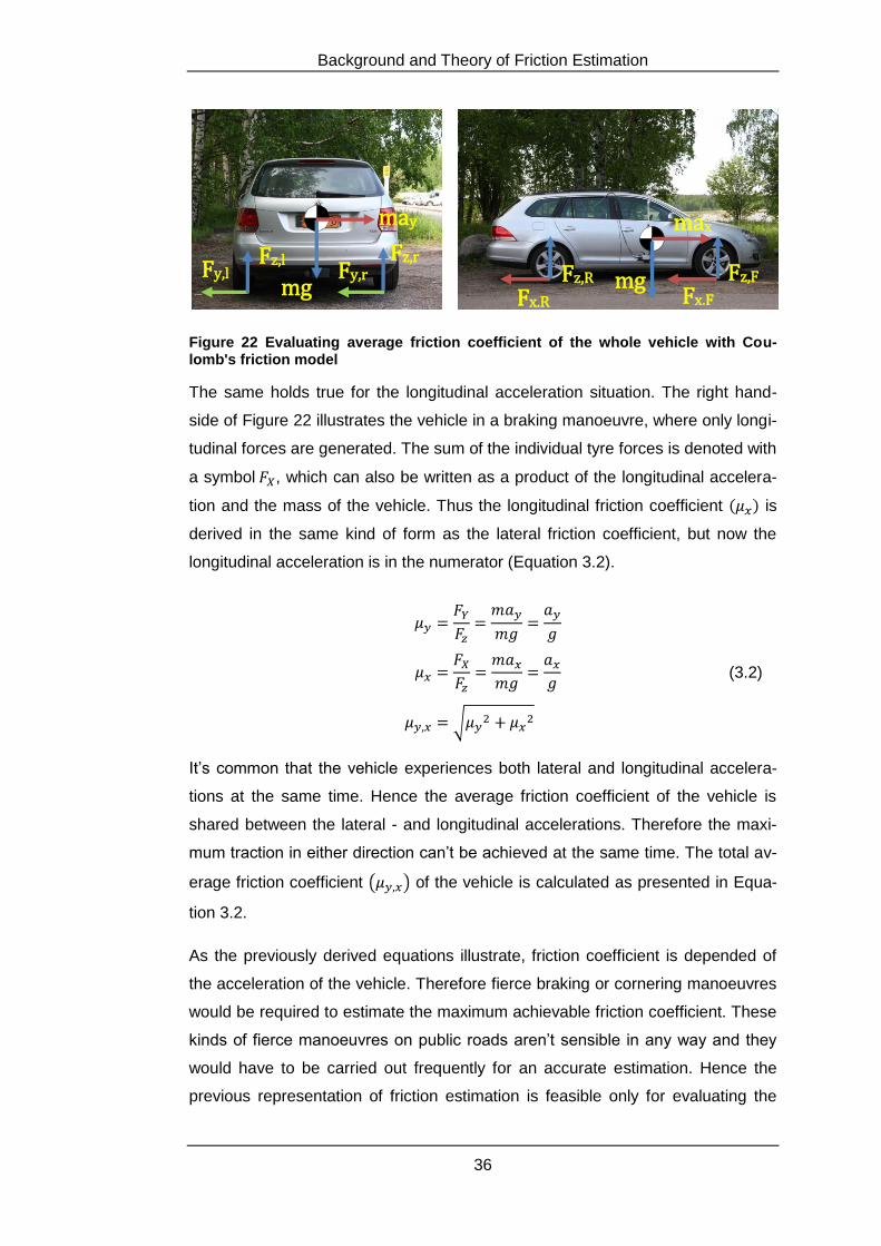
Considering the vehicle as a rigid body moving on a planar surface, the Cou-
lomb’s friction model can be used to estimate the average friction coefficient of
the whole vehicle. The forces that are generated in the tyre-road interfaces are
summed up, which means that the calculated friction coefficient is an average of
these contact points. Thus the expression average friction coefficient. The friction
estimation is divided to pure lateral and longitudinal acceleration situations of the
vehicle. The left-hand side of Figure 22 illustrates the vehicle in a pure cornering
manoeuvre, where each tyre of the vehicle produces a certain amount of lateral
force. The sum of these lateral friction forces is denoted with a symbol , which
can also be written as the product of the centripetal acceleration and the mass of
the vehicle. The normal force of the vehicle can also be written as the product of
the gravitational acceleration and the mass of the vehicle. Thus the average lat-
eral friction coefficient of the vehicle is reduced to a ratio between the lateral
- and the gravitational acceleration (Equation 3.2).
Figure 21 Coulomb’s friction model
Fapplied
µFz
Fz
Background and Theory of Friction Estimation
36
Figure 22 Evaluating average friction coefficient of the whole vehicle with Cou-lomb's friction model
The same holds true for the longitudinal acceleration situation. The right hand-
side of Figure 22 illustrates the vehicle in a braking manoeuvre, where only longi-
tudinal forces are generated. The sum of the individual tyre forces is denoted with
a symbol , which can also be written as a product of the longitudinal accelera-
tion and the mass of the vehicle. Thus the longitudinal friction coefficient is
derived in the same kind of form as the lateral friction coefficient, but now the
longitudinal acceleration is in the numerator (Equation 3.2).
(3.2)
It’s common that the vehicle experiences both lateral and longitudinal accelera-
tions at the same time. Hence the average friction coefficient of the vehicle is
shared between the lateral - and longitudinal accelerations. Therefore the maxi-
mum traction in either direction can’t be achieved at the same time. The total av-
erage friction coefficient of the vehicle is calculated as presented in Equa-
tion 3.2.
As the previously derived equations illustrate, friction coefficient is depended of
the acceleration of the vehicle. Therefore fierce braking or cornering manoeuvres
would be required to estimate the maximum achievable friction coefficient. These
kinds of fierce manoeuvres on public roads aren’t sensible in any way and they
would have to be carried out frequently for an accurate estimation. Hence the
previous representation of friction estimation is feasible only for evaluating the
Fx,R Fx,F mg
Fy,l Fy,r mg
may max
Fz,l Fz,r Fz,F Fz,R
Background and Theory of Friction Estimation
37
friction coefficient that is currently used. Another downside of the previous repre-
sentation of friction estimation is that it doesn’t take into consideration the friction
situation of the individual tyres.
3.2.2 Terminology
The terminology concerned in friction coefficients can be confusing, because dif-
ferent studies have used various terms signifying the same things. Hence the
terms used in this work are defined as follows [10].
Friction used
Friction potential
Friction available
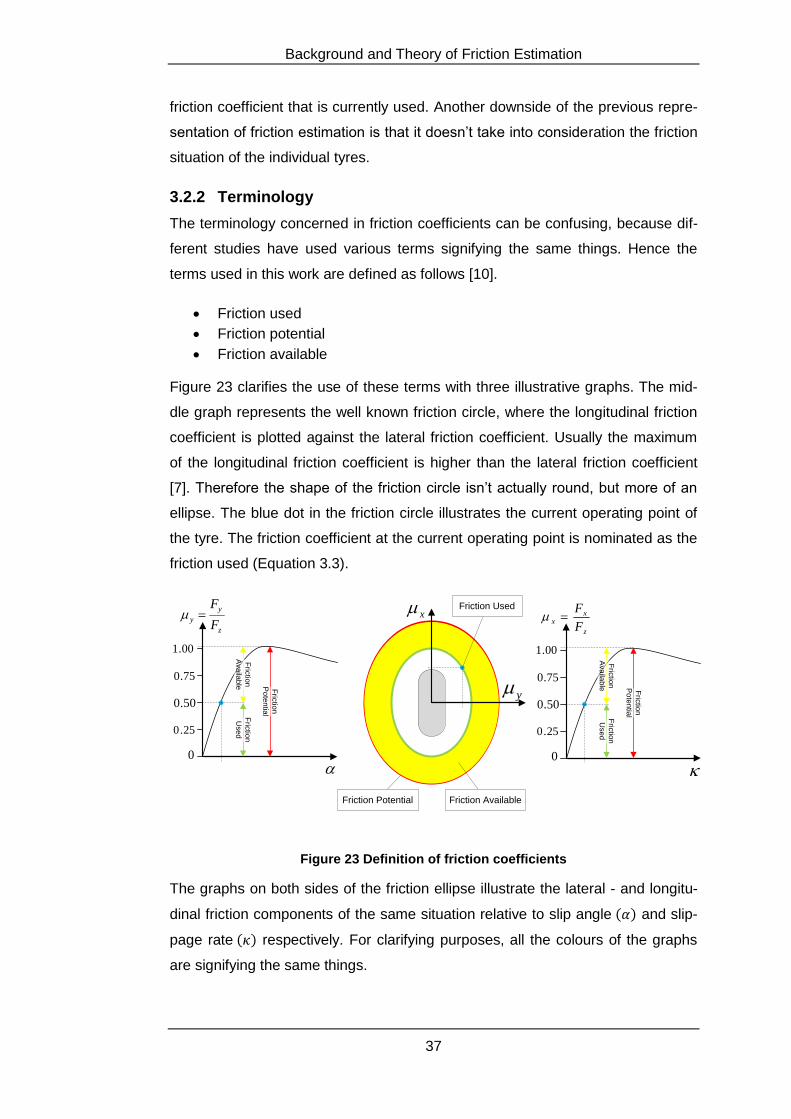
Figure 23 clarifies the use of these terms with three illustrative graphs. The mid-
dle graph represents the well known friction circle, where the longitudinal friction
coefficient is plotted against the lateral friction coefficient. Usually the maximum
of the longitudinal friction coefficient is higher than the lateral friction coefficient
[7]. Therefore the shape of the friction circle isn’t actually round, but more of an
ellipse. The blue dot in the friction circle illustrates the current operating point of
the tyre. The friction coefficient at the current operating point is nominated as the
friction used (Equation 3.3).
z
xx
F
F
0
25.0
50.0
75.0
00.1
Fric
tion
Po
ten
tialF
rictio
n
Use
d
Fric
tion
Ava
ilab
le
x
y
Friction Potential
Friction Used
Friction Available
z
y
yF
F
0
25.0
50.0
75.0
00.1
Fric
tion
Po
ten
tialF
rictio
n
Use
d
Fric
tion
Ava
ilab
le
Figure 23 Definition of friction coefficients
The graphs on both sides of the friction ellipse illustrate the lateral - and longitu-
dinal friction components of the same situation relative to slip angle and slip-
page rate respectively. For clarifying purposes, all the colours of the graphs
are signifying the same things.
Background and Theory of Friction Estimation
38
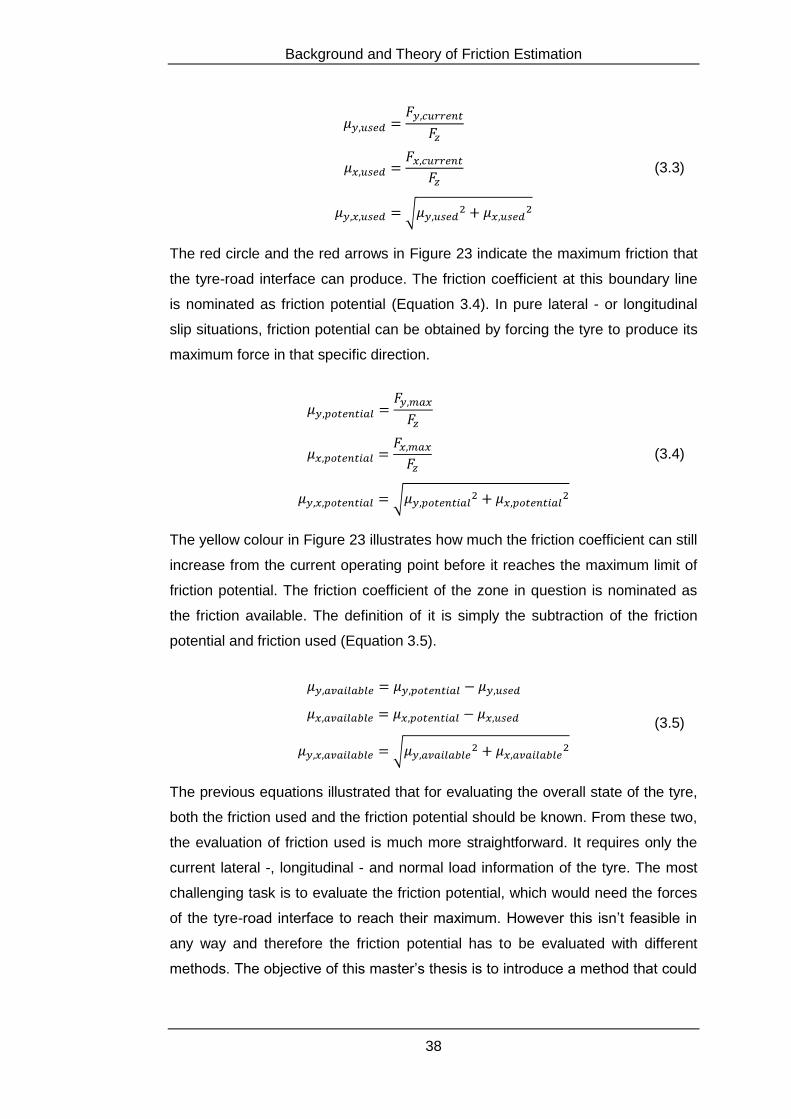
(3.3)
The red circle and the red arrows in Figure 23 indicate the maximum friction that
the tyre-road interface can produce. The friction coefficient at this boundary line
is nominated as friction potential (Equation 3.4). In pure lateral - or longitudinal
slip situations, friction potential can be obtained by forcing the tyre to produce its
maximum force in that specific direction.
(3.4)
The yellow colour in Figure 23 illustrates how much the friction coefficient can still
increase from the current operating point before it reaches the maximum limit of
friction potential. The friction coefficient of the zone in question is nominated as
the friction available. The definition of it is simply the subtraction of the friction
potential and friction used (Equation 3.5).
(3.5)
The previous equations illustrated that for evaluating the overall state of the tyre,
both the friction used and the friction potential should be known. From these two,
the evaluation of friction used is much more straightforward. It requires only the
current lateral -, longitudinal - and normal load information of the tyre. The most
challenging task is to evaluate the friction potential, which would need the forces
of the tyre-road interface to reach their maximum. However this isn’t feasible in
any way and therefore the friction potential has to be evaluated with different
methods. The objective of this master’s thesis is to introduce a method that could
Background and Theory of Friction Estimation
39
estimate the friction potential in a pure lateral slip situation. Thus no longitudinal
forces are produced in the tyre-road interface.
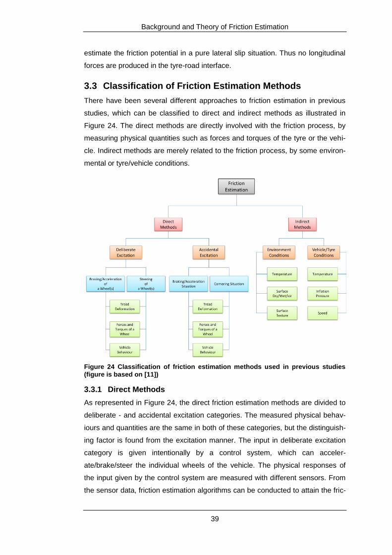
3.3 Classification of Friction Estimation Methods
There have been several different approaches to friction estimation in previous
studies, which can be classified to direct and indirect methods as illustrated in
Figure 24. The direct methods are directly involved with the friction process, by
measuring physical quantities such as forces and torques of the tyre or the vehi-
cle. Indirect methods are merely related to the friction process, by some environ-
mental or tyre/vehicle conditions.
Figure 24 Classification of friction estimation methods used in previous studies (figure is based on [11])
3.3.1 Direct Methods
As represented in Figure 24, the direct friction estimation methods are divided to
deliberate - and accidental excitation categories. The measured physical behav-
iours and quantities are the same in both of these categories, but the distinguish-
ing factor is found from the excitation manner. The input in deliberate excitation
category is given intentionally by a control system, which can acceler-
ate/brake/steer the individual wheels of the vehicle. The physical responses of
the input given by the control system are measured with different sensors. From
the sensor data, friction estimation algorithms can be conducted to attain the fric-
Background and Theory of Friction Estimation
40
tion used and - potential values. Although deliberate excitation methods provide
accurate estimates for friction, they hold major drawbacks. The disadvantages
arise from the fact that the deliberate excitation of the wheels has a significant
influence to vehicle dynamics and therefore to safety and driving dynamics. Also
an additional tyre wear is introduced, which involves energy loss and therefore
increase to the fuel consumption. Thus the use of deliberate excitation methods
can be accepted only for research purposes.
Feasible friction estimation methods are found in the accidental excitation cate-
gory. The inputs in this category are generated by the normal driving manoeu-
vres. Therefore no additional tyre wear or influences to the driving dynamics are
created. However since the friction estimation depends of the inputs given by the
driver, it’s valid only, if there actually exists excitation. Also for accurate friction
estimation the magnitude of the excitation has to be sufficient. Therefore draw-
backs exist, but they are still small compared to deliberate excitation methods.
Since common trips with a vehicle include several cornering situations, it gives
potential circumstances for friction estimation. Therefore this master’s thesis is
concerned with the cornering situation of the accidental excitation methods.
The actual measurements of the physical responses of the inputs can be con-
ducted with three different methods, which are illustrated with green rectangular
boxes in Figure 24. The first method is to measure the deforma-
tions/accelerations of the tyre tread or inner liner. The second method considers
the wheel and the tyre as one packet, which forces and torques are measured.
The third method examines the behaviour of the whole vehicle, which includes
measurements of accelerations and angular -/translational velocities. All of these
methods have been investigated in previous studies to some extent. The focus of
this work is in the second method, measuring the forces and torques of the whole
wheel.
3.3.2 Indirect Methods
Indirect methods aren’t strictly involved with the friction process, but somehow
related to it. Therefore the accuracy of the friction estimation isn’t as good as with
direct methods. However studies have been performed to estimate friction from
environment - and tyre/vehicle conditions. As mentioned previously the traction
between the tyre-road interface is depended of the surface texture quality
(macro-/microroughness), surface conditions (dry/wet/ice) and surface tempera-
Background and Theory of Friction Estimation
41
ture. Therefore these factors can be utilised to estimate friction potential. Espe-
cially optical sensors have been studied for distinguishing the surface conditions.
The advantage of these optical sensors is that they can be positioned to observe
the upcoming surface. Hence the alterations of surface conditions are updated
before the actual contact.
Conditions of the vehicle and the tyre can also be exploited to friction estimation.
E.g. the temperature - and the inflation pressure of tyre are related to the friction
process. The influence of these factors to friction is however limited and the al-
teration of them can be small. Therefore making the friction estimation difficult
and impairing the accuracy.
3.4 Previous Studies
There have been several studies, which have approached the topic of friction
potential estimation with exploiting the information of self aligning torque and lat-
eral force of the tyre. One of the first studies that utilized self aligning torque for
friction estimation was conducted in the Netherlands by Wim R. Pasterkamp. He
assembled a strain gauge in the lower ball joint of the transverse control arm for
evaluating the lateral force of the front tyre. The self aligning torque of the tyre
was attained by measuring the force of the tie rod with a load cell. The vertical
load of the tyre was evaluated by measuring the sway angle of the transverse
control arm. Two different friction estimation methods were implemented. The
first friction estimation method utilized look-up tables and the second neural net-
works. The effect of two different tyre models was also experimented. The first
one was the brush tyre model, which is also used in this master’s thesis and the
other one was the Magic Formula tyre model. Results showed that the imple-
mented estimation methods had potential and thus gave also motivation for this
master’s thesis. [11]
Another similar study performed by The University of Michigan, demonstrated
that the self aligning torque can be exploited to rather accurate friction potential -
and slip angle estimation. For more in-depth description of the estimation meth-
ods see [12].
The self aligning torque is also available at the steering wheel axis and can there-
fore be measured from there. Mitsubishi Electric has conducted a study, where
they have exploited the electronic power steering system as a sensor for estimat-
Background and Theory of Friction Estimation
42
ing the friction potential of the tyre-road interface. This rather simple and cost
effective method showed good accuracy and robustness for the estimation. A
more detailed description can be found from [13].
The researchers in the University of Stanford have also devoted themselves to
several studies, where they have utilized the self aligning torque information to
estimation of friction potential and slip angle. In [14] an algorithm is introduced,
which exploits the steering torque information from the steer-by-wire system for
evaluating the cornering stiffness of the tyre and the friction potential of the tyre-
road interface. The slip angle of the tyre in the same study is derived from
GPS/INS measurements. Another study from the same University utilized the
pneumatic trail information of the self aligning torque for estimating the peak lat-
eral force ( ) and the slip angle of the tyre. This particular estimation method
doesn’t require the knowledge of the normal force of the tyre. More detailed
presentation of this study can be found from [15].
A Swedish Intelligent Vehicle Safety Systems (IVSS) programme has investi-
gated different approaches for evaluating the friction potential of the tyre-road
interface [16]. One part of this study was devoted to estimating friction potential
by utilizing the self aligning torque together with the lateral force of the tyre. The
employed algorithms indicated that a reliable estimate of friction potential re-
quired a lateral acceleration of around 0.3 g. More about the issued friction esti-
mation method together with the other methods concerned in this study is avail-
able in [16].
3.5 Conclusions of this Chapter
The friction forces generated between two rigid bodies are commonly modelled
with the Coulomb’s friction model. It suggests that the produced friction forces
are directly proportional to the normal force, which compresses the bodies to-
gether. The nature of the contact surfaces and the traction quality is represented
with a dimensionless factor called the friction coefficient. It’s defined as the ratio
of the produced friction force and the normal force. Therefore it expresses the
amount of friction force generated in respect to the normal force. Coulomb’s fric-
tion model is commonly accepted and used in engineering, although it has many
generalizations.
Background and Theory of Friction Estimation
43
The evaluation of the overall traction state of the tyre requires the knowledge of
both the friction used and the friction potential. The information of the current lat-
eral -/longitudinal - and normal force of the tyre are the only factors needed for
evaluating the friction used. Thus making it a straightforward task compared to
the evaluation of friction potential, which would require the tyre-road interface to
reach the maximum achievable friction force. These forces are produced only in
fierce braking/acceleration/cornering manoeuvres, which normally occur only in
hazard situations. Therefore the evaluation of friction potential has to be con-
ducted with different methods.
The classification of friction estimation methods can be done according to previ-
ous studies. The main division is done to two categories: direct - and indirect
methods. The first main category includes estimation methods that are directly
involved with the friction process. These methods are implemented by measuring
forces, torques and acceleration of the wheel or the vehicle. The direct methods
are also subdivided to two categories according to the excitation manner (delib-
erate - and accidental excitation). A deliberate toe-in alteration of the front wheels
or a braking of an individual wheel is carried out by a control system in the first
subcategory. The excitations in the other subcategory are produced due to nor-
mal driving manoeuvres. The second main category holds the indirect friction
estimation methods, which are somehow related to the friction process. The ad-
vantage of these methods is that they don’t require any driving inputs for the es-
timation. However since these methods aren’t strictly involved with the friction
process, the accuracy of the estimation can be low.
The friction estimation of this master’s thesis belongs to the direct method cate-
gory and to the accidental excitation subdivision. Concerning only the cornering
situation, where the forces and torques of front wheels are measured.
Research Vehicle and Sensor Equipment
44
4 Research Vehicle and Sensor Equipment
4.1 Introduction
The upcoming subchapters will give an insight to the research vehicle and to the
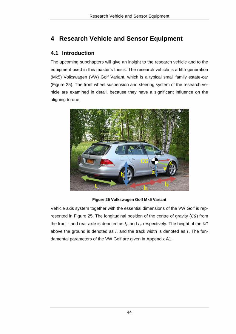
equipment used in this master’s thesis. The research vehicle is a fifth generation
(Mk5) Volkswagen (VW) Golf Variant, which is a typical small family estate-car
(Figure 25). The front wheel suspension and steering system of the research ve-
hicle are examined in detail, because they have a significant influence on the
aligning torque.
Figure 25 Volkswagen Golf Mk5 Variant
Vehicle axis system together with the essential dimensions of the VW Golf is rep-
resented in Figure 25. The longitudinal position of the centre of gravity ( ) from
the front - and rear axle is denoted as and respectively. The height of the
above the ground is denoted as and the track width is denoted as . The fun-
damental parameters of the VW Golf are given in Appendix A1.
CG
h
t lR lF
z y
x
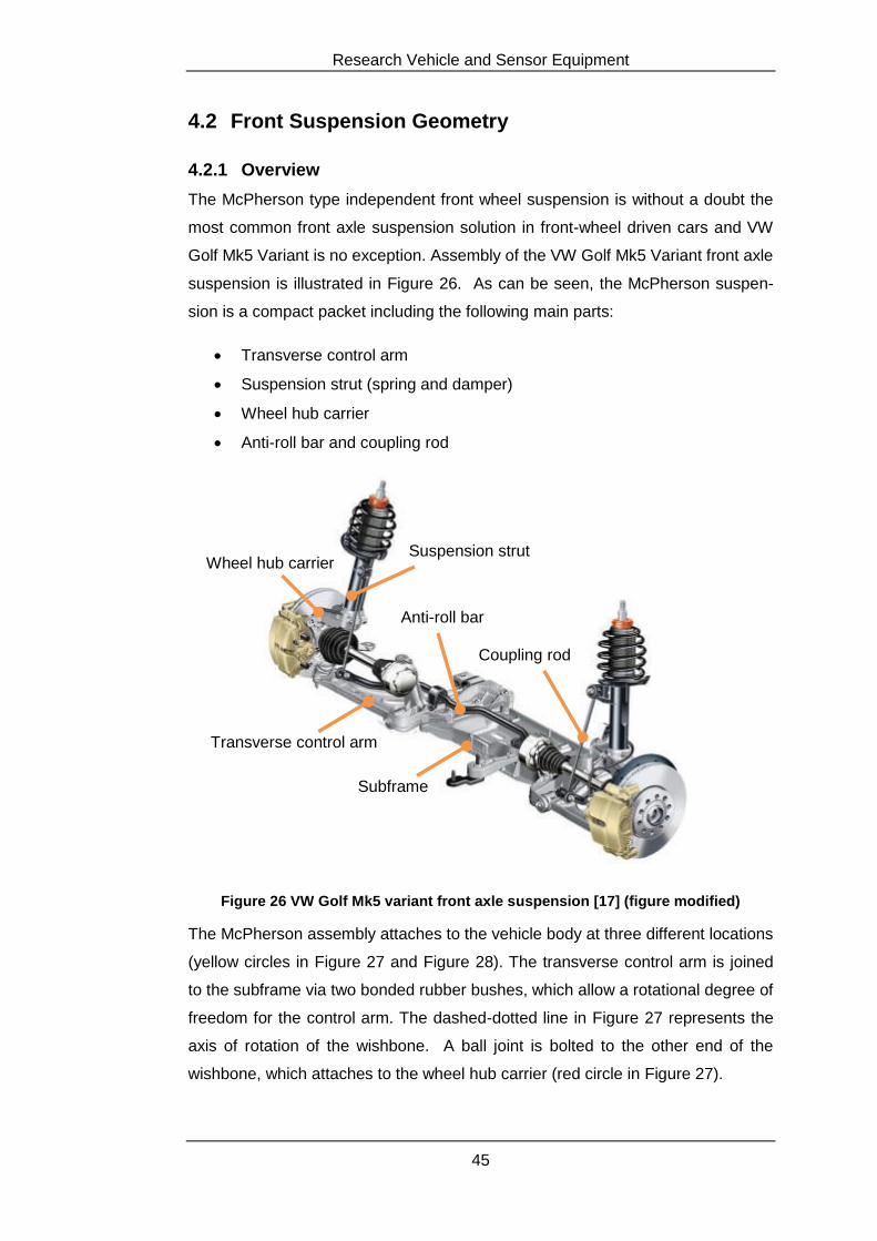
Research Vehicle and Sensor Equipment
45
4.2 Front Suspension Geometry
4.2.1 Overview
The McPherson type independent front wheel suspension is without a doubt the
most common front axle suspension solution in front-wheel driven cars and VW
Golf Mk5 Variant is no exception. Assembly of the VW Golf Mk5 Variant front axle
suspension is illustrated in Figure 26. As can be seen, the McPherson suspen-
sion is a compact packet including the following main parts:
Transverse control arm
Suspension strut (spring and damper)
Wheel hub carrier
Anti-roll bar and coupling rod
Figure 26 VW Golf Mk5 variant front axle suspension [17] (figure modified)
The McPherson assembly attaches to the vehicle body at three different locations
(yellow circles in Figure 27 and Figure 28). The transverse control arm is joined
to the subframe via two bonded rubber bushes, which allow a rotational degree of
freedom for the control arm. The dashed-dotted line in Figure 27 represents the
axis of rotation of the wishbone. A ball joint is bolted to the other end of the
wishbone, which attaches to the wheel hub carrier (red circle in Figure 27).
Wheel hub carrier
Transverse control arm
Suspension strut
Anti-roll bar
Coupling rod
Subframe
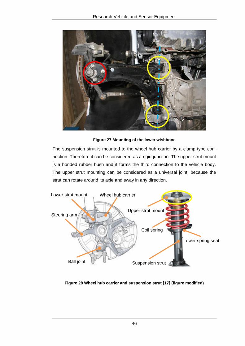
Research Vehicle and Sensor Equipment
46
Figure 27 Mounting of the lower wishbone
The suspension strut is mounted to the wheel hub carrier by a clamp-type con-
nection. Therefore it can be considered as a rigid junction. The upper strut mount
is a bonded rubber bush and it forms the third connection to the vehicle body.
The upper strut mounting can be considered as a universal joint, because the
strut can rotate around its axle and sway in any direction.
Figure 28 Wheel hub carrier and suspension strut [17] (figure modified)
Wheel hub carrier
Lower spring seat
Suspension strut
Coil spring
Ball joint
Steering arm
Lower strut mount
Upper strut mount
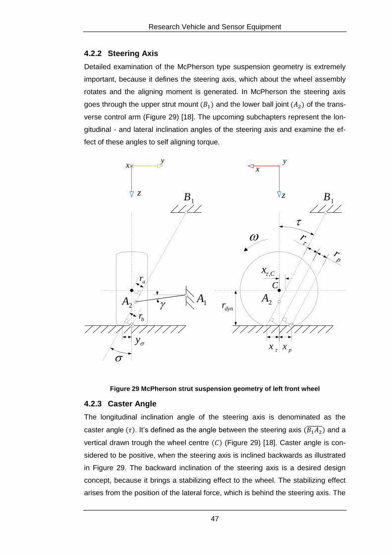
Research Vehicle and Sensor Equipment
47
4.2.2 Steering Axis
Detailed examination of the McPherson type suspension geometry is extremely
important, because it defines the steering axis, which about the wheel assembly
rotates and the aligning moment is generated. In McPherson the steering axis
goes through the upper strut mount and the lower ball joint of the trans-
verse control arm (Figure 29) [18]. The upcoming subchapters represent the lon-
gitudinal - and lateral inclination angles of the steering axis and examine the ef-
fect of these angles to self aligning torque.
1Bz
xy
2A
r
dynr
C
x px
pr
Cx ,
1B
1A2A
xy
z
y
br
ar
Figure 29 McPherson strut suspension geometry of left front wheel
4.2.3 Caster Angle
The longitudinal inclination angle of the steering axis is denominated as the
caster angle . It’s defined as the angle between the steering axis and a
vertical drawn trough the wheel centre (Figure 29) [18]. Caster angle is con-
sidered to be positive, when the steering axis is inclined backwards as illustrated
in Figure 29. The backward inclination of the steering axis is a desired design
concept, because it brings a stabilizing effect to the wheel. The stabilizing effect
arises from the position of the lateral force, which is behind the steering axis. The
Research Vehicle and Sensor Equipment
48
lateral force together with the lever arm generate a torque around the steering
axis, which tries to bring the wheel back to straight a head driving position.
The lateral force lever arm divides to caster trail and pneumatic trail of
the tyre. Considering first only the effect of caster trail, the point of application of
the lateral force is assumed to be at centre point of the contact patch [18]. For
clarifying the terminology, the denomination caster trail signifies the normal dis-
tance from the steering axis to the point of application of the lateral force. The
distance on the ground between the centre point of the contact patch and the
steering axis is denominated as the kinematic caster trail. Obviously the lateral
force lever arm is the shortest distance from the axis of rotation, which is the
caster trail. The length of the caster trail as function of the caster angle can be
evaluated from the suspension geometry by using trigonometric functions. For
the evaluation of the caster trail, two other variables have to be determined and
they are the dynamic rolling radius of the tyre and the caster offset. The dynamic
rolling radius of the tyre is defined as the ratio of the longitudinal velocity and the
angular velocity.
(4.1)
The longitudinal distance between the wheel centre and the steering axis is de-
fined as the caster offset. Typically designers drive for negative caster offset,
which is also the case in the Figure 29. The negative caster offset shortens the
kinematic caster trail, which reduces the steering effects arising from uneven
road surfaces. [18] The length of the caster offset depends of the caster angle
and the distance between the wheel centre and the ball joint. The latter is a static
measure and hence can be evaluated with measurements. Therefore the caster
offset is defined as follows.
(4.2)
Now that the dynamic rolling radius and the caster offset are defined, the caster
trail is evaluated by using trigonometric functions (Figure 29).
(4.3)
However the lateral force distribution of the tyre isn’t symmetrical about the con-
tact patch. It depends of the slip angle, friction coefficient and the normal load
Research Vehicle and Sensor Equipment
49
distribution of the tyre. Therefore the resultant lateral force doesn’t act at centre
point of the contact patch, but at a distance from it called the pneumatic trail. The
length of the pneumatic trail on the ground ( -plane) is derived by using the
brush tyre model, which is discussed thoroughly in the next chapter. Obviously
the force lever arm isn’t the pneumatic trail on the ground, but the normal drawn
from the line, which goes trough the centre point of the contact patch and is par-
allel with the steering axis. The length of this normal can be evaluated with trigo-
nometric functions from the suspension geometry (Figure 29).
(4.4)
The total lateral force lever arm is simply the sum of the caster - and pneumatic
trails.
(4.5)
The total self aligning torque about the steering axis is the product of the lateral
force and the total lateral force lever arm.
(4.6)
The brush tyre model concerns only the self aligning torque that arises from the
pneumatic trail. Therefore the total lateral force lever arm has to be differentiated
to caster - and pneumatic trails in order to subtract the self aligning torque
emerging from the caster trail. For clarifying the equations, the self aligning
torque arising from the caster trail is denoted as and the self aligning torque
arising from the pneumatic trail is denoted as .
(4.7)
The total self aligning torque is evaluated from the tie rod forces and the self
aligning torque arising from the caster trail can be calculated. Thus the desired
self aligning torque emerging from the pneumatic trail is obtained.
(4.8)
As the previous equations have shown, the lateral force lever arm depends of the
caster angle and therefore also the self aligning torque is dependent of it. By ob-
serving the right side of Figure 30, it's obvious that the caster angle alters as
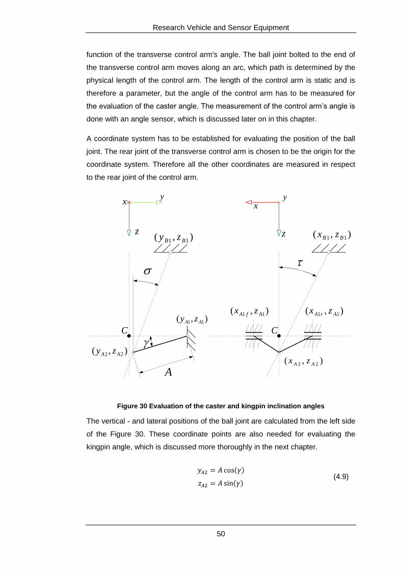
Research Vehicle and Sensor Equipment
50
function of the transverse control arm's angle. The ball joint bolted to the end of
the transverse control arm moves along an arc, which path is determined by the
physical length of the control arm. The length of the control arm is static and is
therefore a parameter, but the angle of the control arm has to be measured for
the evaluation of the caster angle. The measurement of the control arm’s angle is
done with an angle sensor, which is discussed later on in this chapter.
A coordinate system has to be established for evaluating the position of the ball
joint. The rear joint of the transverse control arm is chosen to be the origin for the
coordinate system. Therefore all the other coordinates are measured in respect
to the rear joint of the control arm.
z
xy
C
),( 11 AfA zx ),( 11 ArA zx
),( 22 AA zx
),( 11 BB zx
xy
z
),( 11 BB zy
),( 11 AA zy
),( 22 AA zy
C
A
Figure 30 Evaluation of the caster and kingpin inclination angles
The vertical - and lateral positions of the ball joint are calculated from the left side
of the Figure 30. These coordinate points are also needed for evaluating the
kingpin angle, which is discussed more thoroughly in the next chapter.
(4.9)
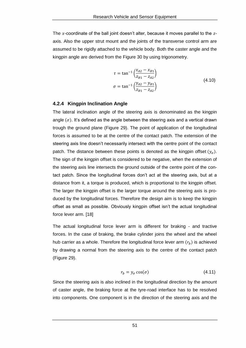
Research Vehicle and Sensor Equipment
51
The -coordinate of the ball joint doesn’t alter, because it moves parallel to the -
axis. Also the upper strut mount and the joints of the transverse control arm are
assumed to be rigidly attached to the vehicle body. Both the caster angle and the
kingpin angle are derived from the Figure 30 by using trigonometry.
(4.10)
4.2.4 Kingpin Inclination Angle
The lateral inclination angle of the steering axis is denominated as the kingpin
angle . It’s defined as the angle between the steering axis and a vertical drawn
trough the ground plane (Figure 29). The point of application of the longitudinal
forces is assumed to be at the centre of the contact patch. The extension of the
steering axis line doesn’t necessarily intersect with the centre point of the contact
patch. The distance between these points is denoted as the kingpin offset .
The sign of the kingpin offset is considered to be negative, when the extension of
the steering axis line intersects the ground outside of the centre point of the con-
tact patch. Since the longitudinal forces don’t act at the steering axis, but at a
distance from it, a torque is produced, which is proportional to the kingpin offset.
The larger the kingpin offset is the larger torque around the steering axis is pro-
duced by the longitudinal forces. Therefore the design aim is to keep the kingpin
offset as small as possible. Obviously kingpin offset isn’t the actual longitudinal
force lever arm. [18]
The actual longitudinal force lever arm is different for braking - and tractive
forces. In the case of braking, the brake cylinder joins the wheel and the wheel
hub carrier as a whole. Therefore the longitudinal force lever arm is achieved
by drawing a normal from the steering axis to the centre of the contact patch
(Figure 29).
(4.11)
Since the steering axis is also inclined in the longitudinal direction by the amount
of caster angle, the braking force at the tyre-road interface has to be resolved
into components. One component is in the direction of the steering axis and the
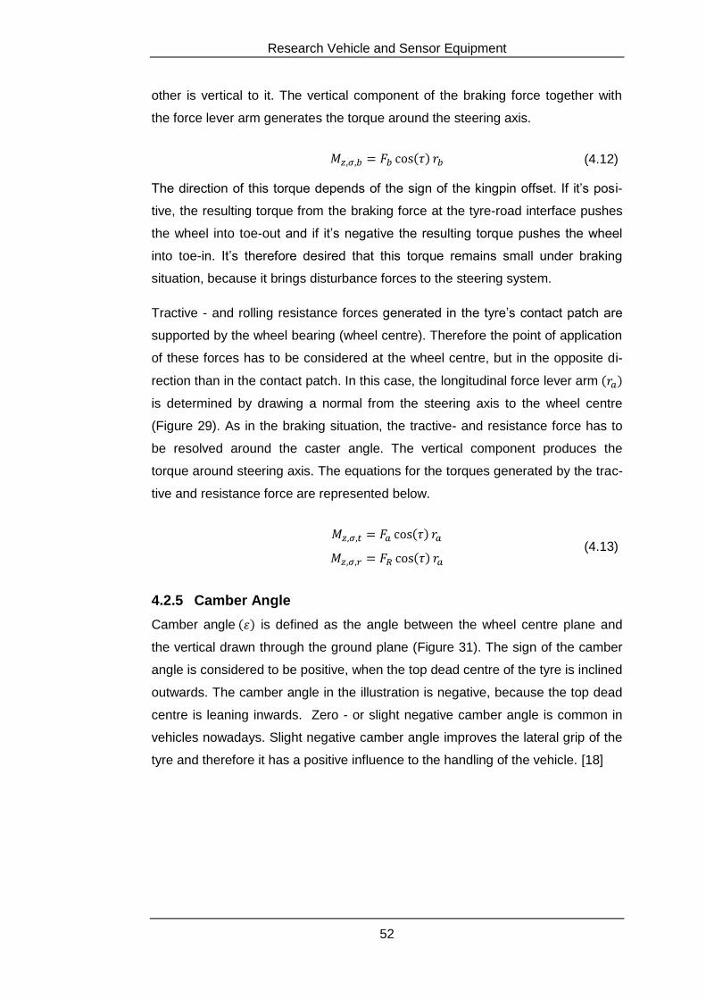
Research Vehicle and Sensor Equipment
52
other is vertical to it. The vertical component of the braking force together with
the force lever arm generates the torque around the steering axis.
(4.12)
The direction of this torque depends of the sign of the kingpin offset. If it’s posi-
tive, the resulting torque from the braking force at the tyre-road interface pushes
the wheel into toe-out and if it’s negative the resulting torque pushes the wheel
into toe-in. It’s therefore desired that this torque remains small under braking
situation, because it brings disturbance forces to the steering system.
Tractive - and rolling resistance forces generated in the tyre’s contact patch are
supported by the wheel bearing (wheel centre). Therefore the point of application
of these forces has to be considered at the wheel centre, but in the opposite di-
rection than in the contact patch. In this case, the longitudinal force lever arm
is determined by drawing a normal from the steering axis to the wheel centre
(Figure 29). As in the braking situation, the tractive- and resistance force has to
be resolved around the caster angle. The vertical component produces the
torque around steering axis. The equations for the torques generated by the trac-
tive and resistance force are represented below.
(4.13)
4.2.5 Camber Angle
Camber angle is defined as the angle between the wheel centre plane and
the vertical drawn through the ground plane (Figure 31). The sign of the camber
angle is considered to be positive, when the top dead centre of the tyre is inclined
outwards. The camber angle in the illustration is negative, because the top dead
centre is leaning inwards. Zero - or slight negative camber angle is common in
vehicles nowadays. Slight negative camber angle improves the lateral grip of the
tyre and therefore it has a positive influence to the handling of the vehicle. [18]
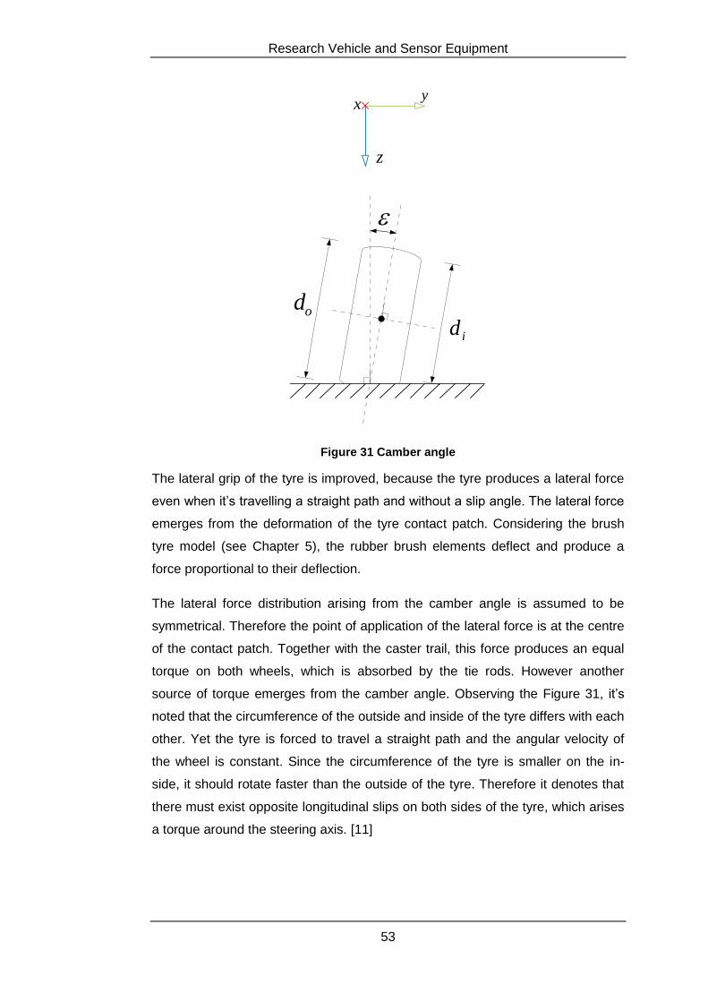
Research Vehicle and Sensor Equipment
53
xy
z
od
id
Figure 31 Camber angle
The lateral grip of the tyre is improved, because the tyre produces a lateral force
even when it’s travelling a straight path and without a slip angle. The lateral force
emerges from the deformation of the tyre contact patch. Considering the brush
tyre model (see Chapter 5), the rubber brush elements deflect and produce a
force proportional to their deflection.
The lateral force distribution arising from the camber angle is assumed to be
symmetrical. Therefore the point of application of the lateral force is at the centre
of the contact patch. Together with the caster trail, this force produces an equal
torque on both wheels, which is absorbed by the tie rods. However another
source of torque emerges from the camber angle. Observing the Figure 31, it’s
noted that the circumference of the outside and inside of the tyre differs with each
other. Yet the tyre is forced to travel a straight path and the angular velocity of
the wheel is constant. Since the circumference of the tyre is smaller on the in-
side, it should rotate faster than the outside of the tyre. Therefore it denotes that
there must exist opposite longitudinal slips on both sides of the tyre, which arises
a torque around the steering axis. [11]
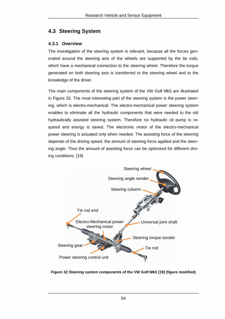
Research Vehicle and Sensor Equipment
54
4.3 Steering System
4.3.1 Overview
The investigation of the steering system is relevant, because all the forces gen-
erated around the steering axis of the wheels are supported by the tie rods,
which have a mechanical connection to the steering wheel. Therefore the torque
generated on both steering axis is transferred to the steering wheel and to the
knowledge of the driver.
The main components of the steering system of the VW Golf Mk5 are illustrated
in Figure 32. The most interesting part of the steering system is the power steer-
ing, which is electro-mechanical. The electro-mechanical power steering system
enables to eliminate all the hydraulic components that were needed to the old
hydraulically assisted steering system. Therefore no hydraulic oil pump is re-
quired and energy is saved. The electronic motor of the electro-mechanical
power steering is actuated only when needed. The assisting force of the steering
depends of the driving speed, the amount of steering force applied and the steer-
ing angle. Thus the amount of assisting force can be optimized for different driv-
ing conditions. [19]
Figure 32 Steering system components of the VW Golf Mk5 [19] (figure modified)
Steering wheel
Steering column
Tie rod
Universal joint shaft
Power steering control unit
Steering gear
Electro-Mechanical power steering motor
Tie rod end
Steering angle sender
Steering torque sender
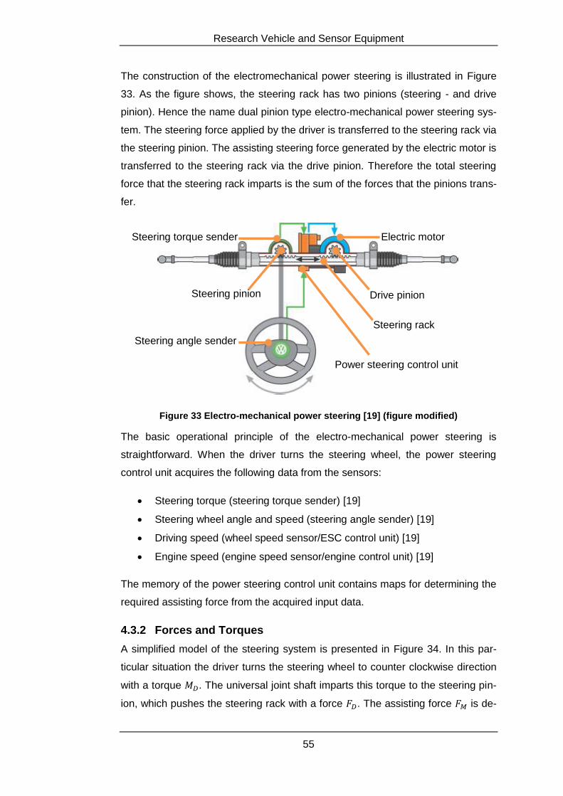
Research Vehicle and Sensor Equipment
55
The construction of the electromechanical power steering is illustrated in Figure
33. As the figure shows, the steering rack has two pinions (steering - and drive
pinion). Hence the name dual pinion type electro-mechanical power steering sys-
tem. The steering force applied by the driver is transferred to the steering rack via
the steering pinion. The assisting steering force generated by the electric motor is
transferred to the steering rack via the drive pinion. Therefore the total steering
force that the steering rack imparts is the sum of the forces that the pinions trans-
fer.
Figure 33 Electro-mechanical power steering [19] (figure modified)
The basic operational principle of the electro-mechanical power steering is
straightforward. When the driver turns the steering wheel, the power steering
control unit acquires the following data from the sensors:
Steering torque (steering torque sender) [19]
Steering wheel angle and speed (steering angle sender) [19]
Driving speed (wheel speed sensor/ESC control unit) [19]
Engine speed (engine speed sensor/engine control unit) [19]
The memory of the power steering control unit contains maps for determining the
required assisting force from the acquired input data.
4.3.2 Forces and Torques
A simplified model of the steering system is presented in Figure 34. In this par-
ticular situation the driver turns the steering wheel to counter clockwise direction
with a torque . The universal joint shaft imparts this torque to the steering pin-
ion, which pushes the steering rack with a force . The assisting force is de-
Drive pinion Steering pinion
Steering rack
Power steering control unit
Electric motor Steering torque sender
Steering angle sender
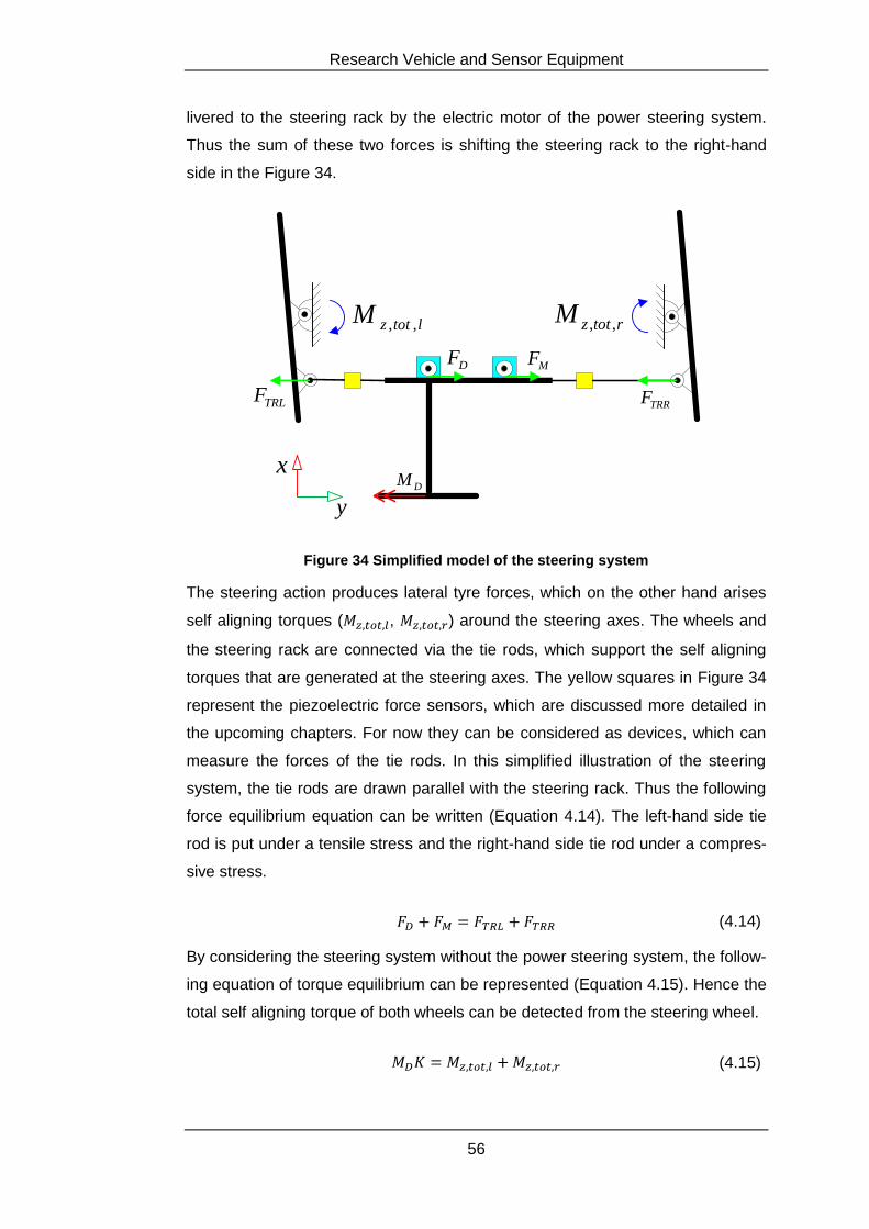
Research Vehicle and Sensor Equipment
56
livered to the steering rack by the electric motor of the power steering system.
Thus the sum of these two forces is shifting the steering rack to the right-hand
side in the Figure 34.
ltotzM ,,
DFMF
TRLFTRRF
DMx
y
rtotzM ,,
Figure 34 Simplified model of the steering system
The steering action produces lateral tyre forces, which on the other hand arises
self aligning torques ( , ) around the steering axes. The wheels and
the steering rack are connected via the tie rods, which support the self aligning
torques that are generated at the steering axes. The yellow squares in Figure 34
represent the piezoelectric force sensors, which are discussed more detailed in
the upcoming chapters. For now they can be considered as devices, which can
measure the forces of the tie rods. In this simplified illustration of the steering
system, the tie rods are drawn parallel with the steering rack. Thus the following
force equilibrium equation can be written (Equation 4.14). The left-hand side tie
rod is put under a tensile stress and the right-hand side tie rod under a compres-
sive stress.
(4.14)
By considering the steering system without the power steering system, the follow-
ing equation of torque equilibrium can be represented (Equation 4.15). Hence the
total self aligning torque of both wheels can be detected from the steering wheel.
(4.15)
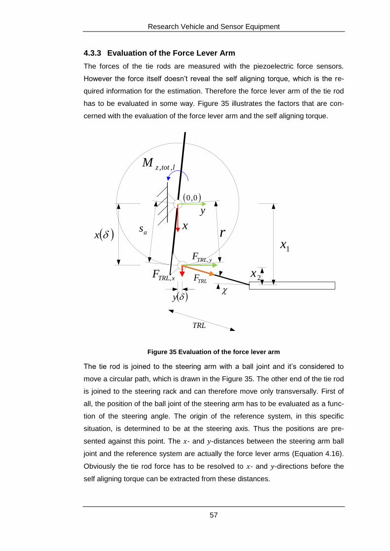
Research Vehicle and Sensor Equipment
57
4.3.3 Evaluation of the Force Lever Arm
The forces of the tie rods are measured with the piezoelectric force sensors.
However the force itself doesn’t reveal the self aligning torque, which is the re-
quired information for the estimation. Therefore the force lever arm of the tie rod
has to be evaluated in some way. Figure 35 illustrates the factors that are con-
cerned with the evaluation of the force lever arm and the self aligning torque.
0,0
x
y
1x x
TRLF
r
y
TRL
2x
yTRLF ,
xTRLF ,
as
ltotzM ,,
Figure 35 Evaluation of the force lever arm
The tie rod is joined to the steering arm with a ball joint and it’s considered to
move a circular path, which is drawn in the Figure 35. The other end of the tie rod
is joined to the steering rack and can therefore move only transversally. First of
all, the position of the ball joint of the steering arm has to be evaluated as a func-
tion of the steering angle. The origin of the reference system, in this specific
situation, is determined to be at the steering axis. Thus the positions are pre-
sented against this point. The - and -distances between the steering arm ball
joint and the reference system are actually the force lever arms (Equation 4.16).
Obviously the tie rod force has to be resolved to - and -directions before the
self aligning torque can be extracted from these distances.
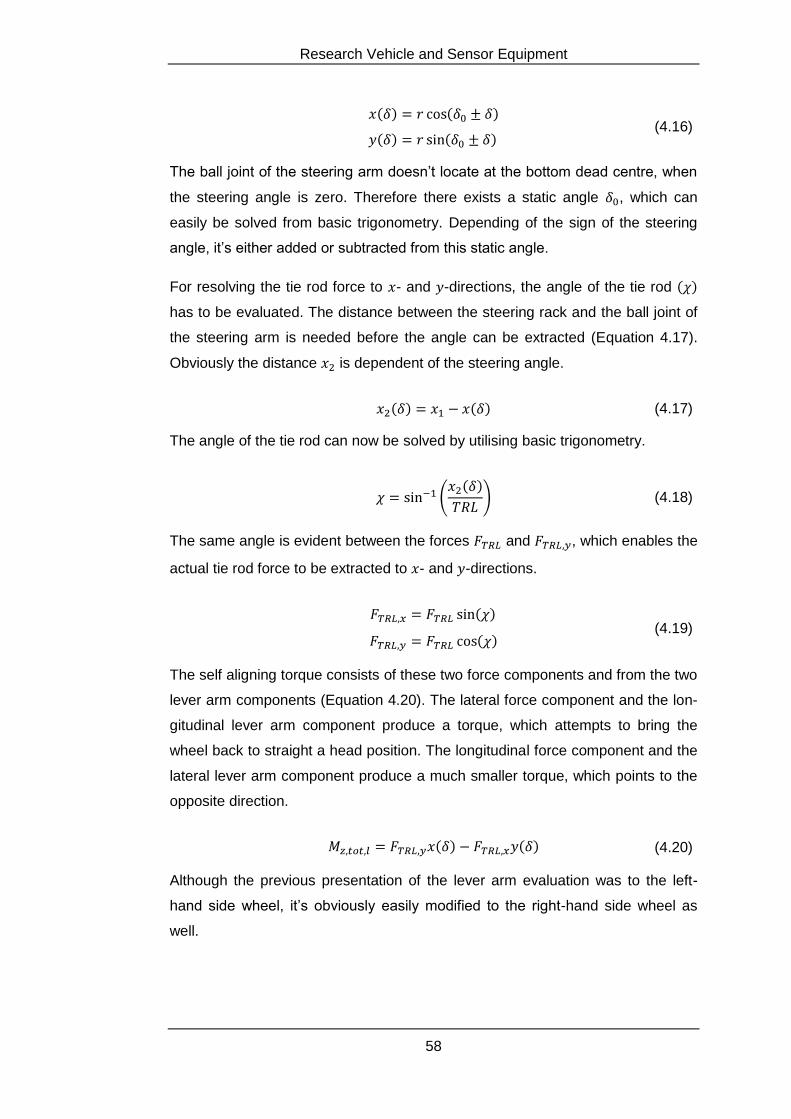
Research Vehicle and Sensor Equipment
58
(4.16)
The ball joint of the steering arm doesn’t locate at the bottom dead centre, when
the steering angle is zero. Therefore there exists a static angle , which can
easily be solved from basic trigonometry. Depending of the sign of the steering
angle, it’s either added or subtracted from this static angle.
For resolving the tie rod force to - and -directions, the angle of the tie rod
has to be evaluated. The distance between the steering rack and the ball joint of
the steering arm is needed before the angle can be extracted (Equation 4.17).
Obviously the distance is dependent of the steering angle.
(4.17)
The angle of the tie rod can now be solved by utilising basic trigonometry.
(4.18)
The same angle is evident between the forces and , which enables the
actual tie rod force to be extracted to - and -directions.
(4.19)
The self aligning torque consists of these two force components and from the two
lever arm components (Equation 4.20). The lateral force component and the lon-
gitudinal lever arm component produce a torque, which attempts to bring the
wheel back to straight a head position. The longitudinal force component and the
lateral lever arm component produce a much smaller torque, which points to the
opposite direction.
(4.20)
Although the previous presentation of the lever arm evaluation was to the left-
hand side wheel, it’s obviously easily modified to the right-hand side wheel as
well.
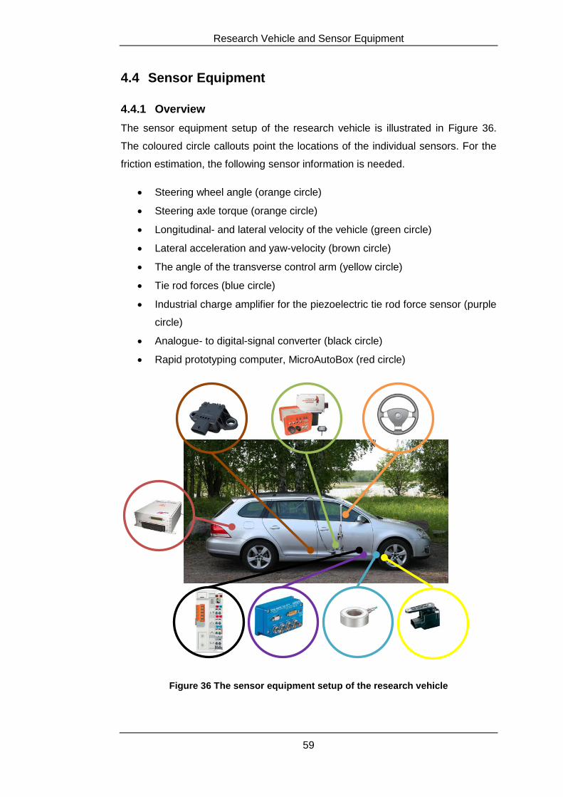
Research Vehicle and Sensor Equipment
59
4.4 Sensor Equipment
4.4.1 Overview
The sensor equipment setup of the research vehicle is illustrated in Figure 36.
The coloured circle callouts point the locations of the individual sensors. For the
friction estimation, the following sensor information is needed.
Steering wheel angle (orange circle)
Steering axle torque (orange circle)
Longitudinal- and lateral velocity of the vehicle (green circle)
Lateral acceleration and yaw-velocity (brown circle)
The angle of the transverse control arm (yellow circle)
Tie rod forces (blue circle)
Industrial charge amplifier for the piezoelectric tie rod force sensor (purple
circle)
Analogue- to digital-signal converter (black circle)
Rapid prototyping computer, MicroAutoBox (red circle)
Figure 36 The sensor equipment setup of the research vehicle
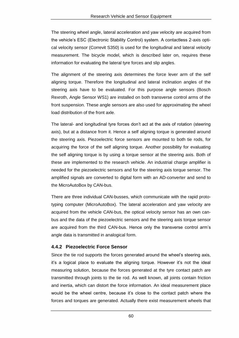
Research Vehicle and Sensor Equipment
60
The steering wheel angle, lateral acceleration and yaw velocity are acquired from
the vehicle’s ESC (Electronic Stability Control) system. A contactless 2-axis opti-
cal velocity sensor (Correvit S350) is used for the longitudinal and lateral velocity
measurement. The bicycle model, which is described later on, requires these
information for evaluating the lateral tyre forces and slip angles.
The alignment of the steering axis determines the force lever arm of the self
aligning torque. Therefore the longitudinal and lateral inclination angles of the
steering axis have to be evaluated. For this purpose angle sensors (Bosch
Rexroth, Angle Sensor WS1) are installed on both transverse control arms of the
front suspension. These angle sensors are also used for approximating the wheel
load distribution of the front axle.
The lateral- and longitudinal tyre forces don’t act at the axis of rotation (steering
axis), but at a distance from it. Hence a self aligning torque is generated around
the steering axis. Piezoelectric force sensors are mounted to both tie rods, for
acquiring the force of the self aligning torque. Another possibility for evaluating
the self aligning torque is by using a torque sensor at the steering axis. Both of
these are implemented to the research vehicle. An industrial charge amplifier is
needed for the piezoelectric sensors and for the steering axis torque sensor. The
amplified signals are converted to digital form with an AD-converter and send to
the MicroAutoBox by CAN-bus.
There are three individual CAN-busses, which communicate with the rapid proto-
typing computer (MicroAutoBox). The lateral acceleration and yaw velocity are
acquired from the vehicle CAN-bus, the optical velocity sensor has an own can-
bus and the data of the piezoelectric sensors and the steering axis torque sensor
are acquired from the third CAN-bus. Hence only the transverse control arm’s
angle data is transmitted in analogical form.
4.4.2 Piezoelectric Force Sensor
Since the tie rod supports the forces generated around the wheel’s steering axis,
it’s a logical place to evaluate the aligning torque. However it’s not the ideal
measuring solution, because the forces generated at the tyre contact patch are
transmitted through joints to the tie rod. As well known, all joints contain friction
and inertia, which can distort the force information. An ideal measurement place
would be the wheel centre, because it’s close to the contact patch where the
forces and torques are generated. Actually there exist measurement wheels that
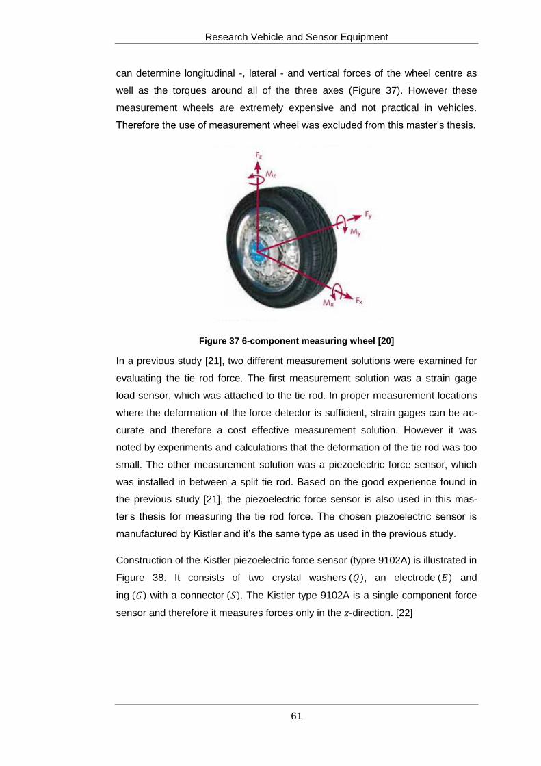
Research Vehicle and Sensor Equipment
61
can determine longitudinal -, lateral - and vertical forces of the wheel centre as
well as the torques around all of the three axes (Figure 37). However these
measurement wheels are extremely expensive and not practical in vehicles.
Therefore the use of measurement wheel was excluded from this master’s thesis.
Figure 37 6-component measuring wheel [20]
In a previous study [21], two different measurement solutions were examined for
evaluating the tie rod force. The first measurement solution was a strain gage
load sensor, which was attached to the tie rod. In proper measurement locations
where the deformation of the force detector is sufficient, strain gages can be ac-
curate and therefore a cost effective measurement solution. However it was
noted by experiments and calculations that the deformation of the tie rod was too
small. The other measurement solution was a piezoelectric force sensor, which
was installed in between a split tie rod. Based on the good experience found in
the previous study [21], the piezoelectric force sensor is also used in this mas-
ter’s thesis for measuring the tie rod force. The chosen piezoelectric sensor is
manufactured by Kistler and it’s the same type as used in the previous study.
Construction of the Kistler piezoelectric force sensor (typre 9102A) is illustrated in
Figure 38. It consists of two crystal washers , an electrode and
ing with a connector . The Kistler type 9102A is a single component force
sensor and therefore it measures forces only in the -direction. [22]
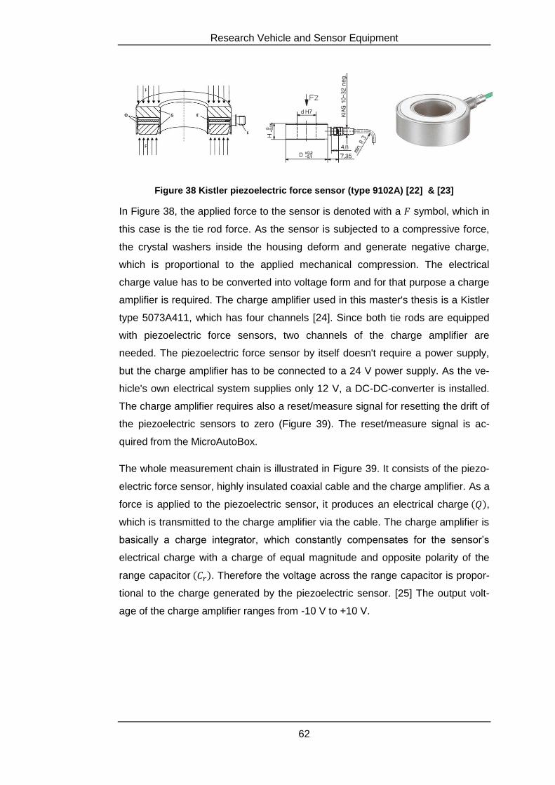
Research Vehicle and Sensor Equipment
62
Figure 38 Kistler piezoelectric force sensor (type 9102A) [22] & [23]
In Figure 38, the applied force to the sensor is denoted with a symbol, which in
this case is the tie rod force. As the sensor is subjected to a compressive force,
the crystal washers inside the housing deform and generate negative charge,
which is proportional to the applied mechanical compression. The electrical
charge value has to be converted into voltage form and for that purpose a charge
amplifier is required. The charge amplifier used in this master's thesis is a Kistler
type 5073A411, which has four channels [24]. Since both tie rods are equipped
with piezoelectric force sensors, two channels of the charge amplifier are
needed. The piezoelectric force sensor by itself doesn't require a power supply,
but the charge amplifier has to be connected to a 24 V power supply. As the ve-
hicle's own electrical system supplies only 12 V, a DC-DC-converter is installed.
The charge amplifier requires also a reset/measure signal for resetting the drift of
the piezoelectric sensors to zero (Figure 39). The reset/measure signal is ac-
quired from the MicroAutoBox.
The whole measurement chain is illustrated in Figure 39. It consists of the piezo-
electric force sensor, highly insulated coaxial cable and the charge amplifier. As a
force is applied to the piezoelectric sensor, it produces an electrical charge ,
which is transmitted to the charge amplifier via the cable. The charge amplifier is
basically a charge integrator, which constantly compensates for the sensor’s
electrical charge with a charge of equal magnitude and opposite polarity of the
range capacitor . Therefore the voltage across the range capacitor is propor-
tional to the charge generated by the piezoelectric sensor. [25] The output volt-
age of the charge amplifier ranges from -10 V to +10 V.
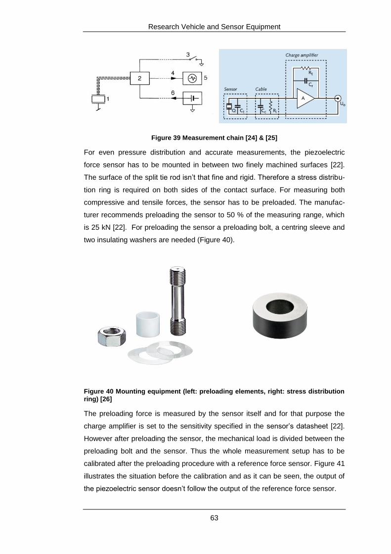
Research Vehicle and Sensor Equipment
63
Figure 39 Measurement chain [24] & [25]
For even pressure distribution and accurate measurements, the piezoelectric
force sensor has to be mounted in between two finely machined surfaces [22].
The surface of the split tie rod isn’t that fine and rigid. Therefore a stress distribu-
tion ring is required on both sides of the contact surface. For measuring both
compressive and tensile forces, the sensor has to be preloaded. The manufac-
turer recommends preloading the sensor to 50 % of the measuring range, which
is 25 kN [22]. For preloading the sensor a preloading bolt, a centring sleeve and
two insulating washers are needed (Figure 40).
Figure 40 Mounting equipment (left: preloading elements, right: stress distribution ring) [26]
The preloading force is measured by the sensor itself and for that purpose the
charge amplifier is set to the sensitivity specified in the sensor’s datasheet [22].
However after preloading the sensor, the mechanical load is divided between the
preloading bolt and the sensor. Thus the whole measurement setup has to be
calibrated after the preloading procedure with a reference force sensor. Figure 41
illustrates the situation before the calibration and as it can be seen, the output of
the piezoelectric sensor doesn’t follow the output of the reference force sensor.
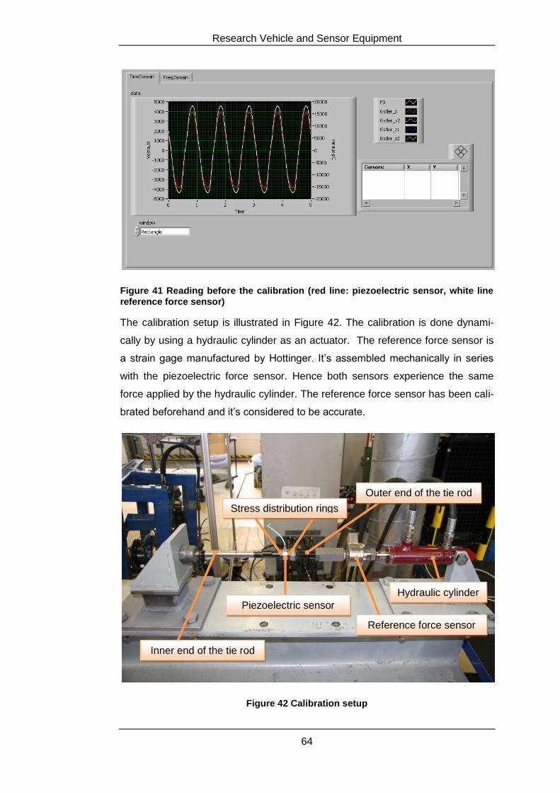
Research Vehicle and Sensor Equipment
64
Figure 41 Reading before the calibration (red line: piezoelectric sensor, white line reference force sensor)
The calibration setup is illustrated in Figure 42. The calibration is done dynami-
cally by using a hydraulic cylinder as an actuator. The reference force sensor is
a strain gage manufactured by Hottinger. It’s assembled mechanically in series
with the piezoelectric force sensor. Hence both sensors experience the same
force applied by the hydraulic cylinder. The reference force sensor has been cali-
brated beforehand and it’s considered to be accurate.
Figure 42 Calibration setup
Stress distribution rings
Piezoelectric sensor
Hydraulic cylinder
Reference force sensor
Inner end of the tie rod
Outer end of the tie rod
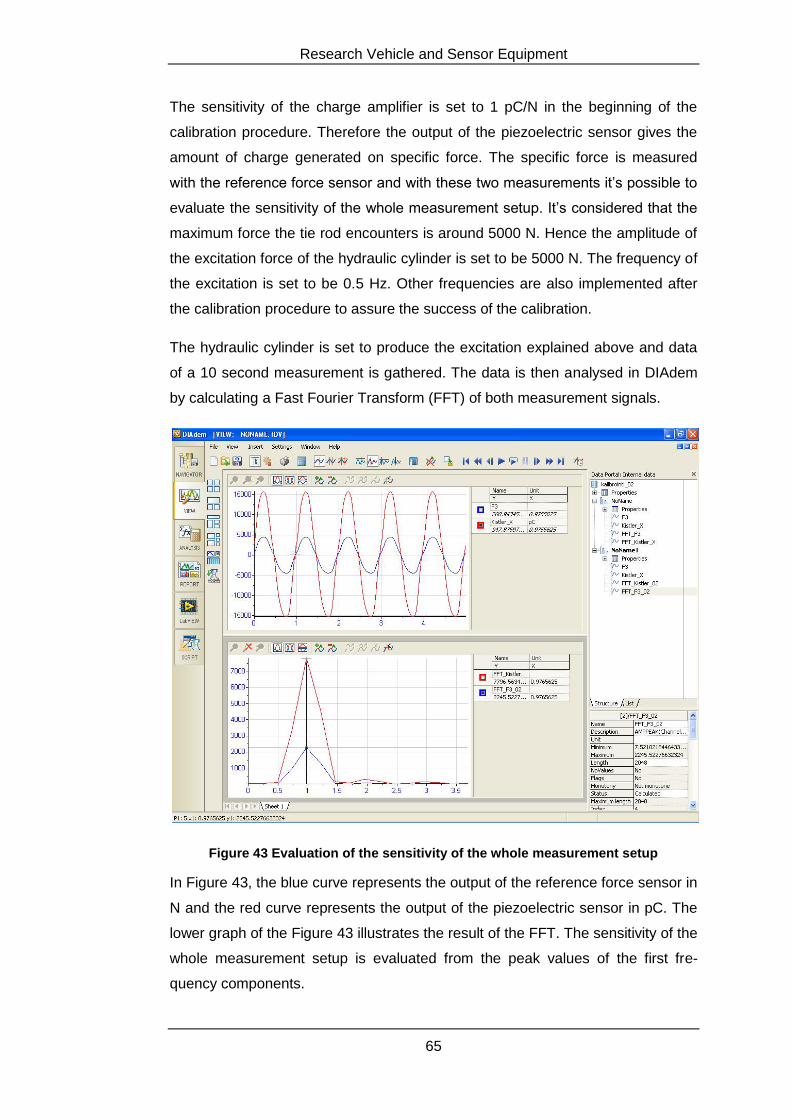
Research Vehicle and Sensor Equipment
65
The sensitivity of the charge amplifier is set to 1 pC/N in the beginning of the
calibration procedure. Therefore the output of the piezoelectric sensor gives the
amount of charge generated on specific force. The specific force is measured
with the reference force sensor and with these two measurements it’s possible to
evaluate the sensitivity of the whole measurement setup. It’s considered that the
maximum force the tie rod encounters is around 5000 N. Hence the amplitude of
the excitation force of the hydraulic cylinder is set to be 5000 N. The frequency of
the excitation is set to be 0.5 Hz. Other frequencies are also implemented after
the calibration procedure to assure the success of the calibration.
The hydraulic cylinder is set to produce the excitation explained above and data
of a 10 second measurement is gathered. The data is then analysed in DIAdem
by calculating a Fast Fourier Transform (FFT) of both measurement signals.
Figure 43 Evaluation of the sensitivity of the whole measurement setup
In Figure 43, the blue curve represents the output of the reference force sensor in
N and the red curve represents the output of the piezoelectric sensor in pC. The
lower graph of the Figure 43 illustrates the result of the FFT. The sensitivity of the
whole measurement setup is evaluated from the peak values of the first fre-
quency components.
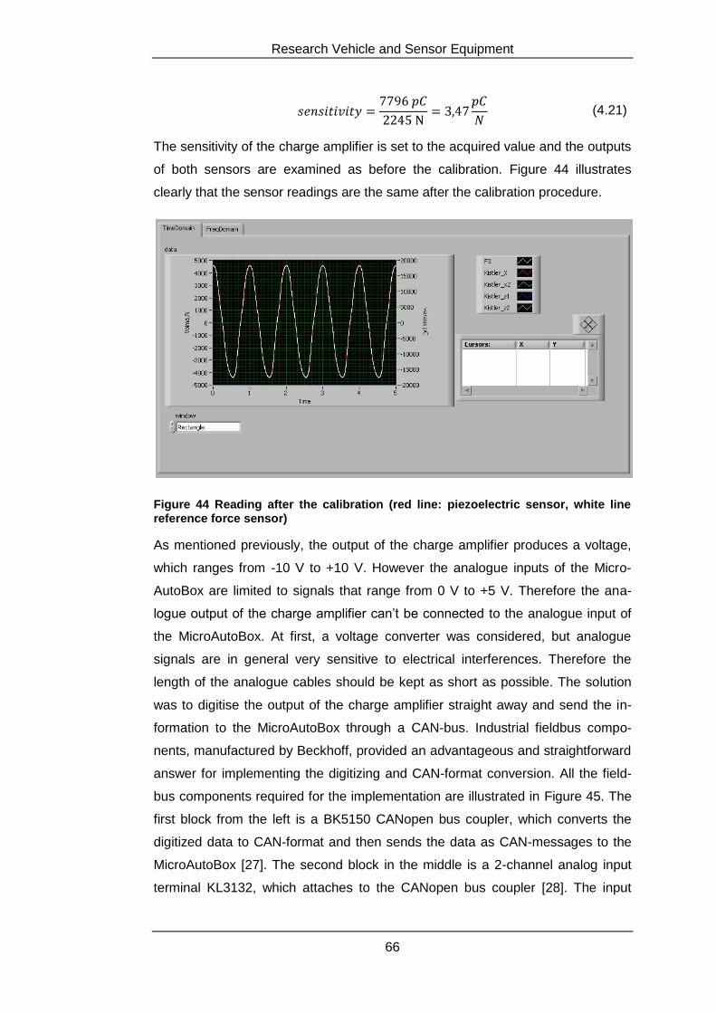
Research Vehicle and Sensor Equipment
66
(4.21)
The sensitivity of the charge amplifier is set to the acquired value and the outputs
of both sensors are examined as before the calibration. Figure 44 illustrates
clearly that the sensor readings are the same after the calibration procedure.
Figure 44 Reading after the calibration (red line: piezoelectric sensor, white line reference force sensor)
As mentioned previously, the output of the charge amplifier produces a voltage,
which ranges from -10 V to +10 V. However the analogue inputs of the Micro-
AutoBox are limited to signals that range from 0 V to +5 V. Therefore the ana-
logue output of the charge amplifier can’t be connected to the analogue input of
the MicroAutoBox. At first, a voltage converter was considered, but analogue
signals are in general very sensitive to electrical interferences. Therefore the
length of the analogue cables should be kept as short as possible. The solution
was to digitise the output of the charge amplifier straight away and send the in-
formation to the MicroAutoBox through a CAN-bus. Industrial fieldbus compo-
nents, manufactured by Beckhoff, provided an advantageous and straightforward
answer for implementing the digitizing and CAN-format conversion. All the field-
bus components required for the implementation are illustrated in Figure 45. The
first block from the left is a BK5150 CANopen bus coupler, which converts the
digitized data to CAN-format and then sends the data as CAN-messages to the
MicroAutoBox [27]. The second block in the middle is a 2-channel analog input
terminal KL3132, which attaches to the CANopen bus coupler [28]. The input
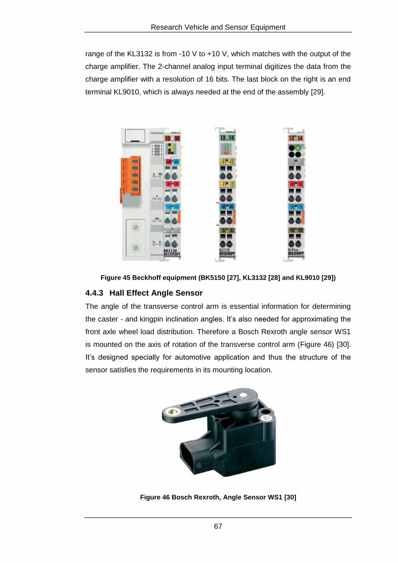
Research Vehicle and Sensor Equipment
67
range of the KL3132 is from -10 V to +10 V, which matches with the output of the
charge amplifier. The 2-channel analog input terminal digitizes the data from the
charge amplifier with a resolution of 16 bits. The last block on the right is an end
terminal KL9010, which is always needed at the end of the assembly [29].
Figure 45 Beckhoff equipment (BK5150 [27], KL3132 [28] and KL9010 [29])
4.4.3 Hall Effect Angle Sensor
The angle of the transverse control arm is essential information for determining
the caster - and kingpin inclination angles. It’s also needed for approximating the
front axle wheel load distribution. Therefore a Bosch Rexroth angle sensor WS1
is mounted on the axis of rotation of the transverse control arm (Figure 46) [30].
It’s designed specially for automotive application and thus the structure of the
sensor satisfies the requirements in its mounting location.
Figure 46 Bosch Rexroth, Angle Sensor WS1 [30]
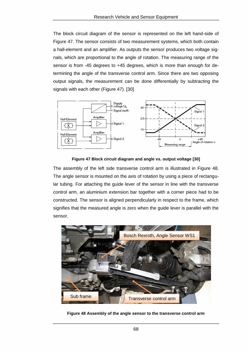
Research Vehicle and Sensor Equipment
68
The block circuit diagram of the sensor is represented on the left hand-side of
Figure 47. The sensor consists of two measurement systems, which both contain
a hall-element and an amplifier. As outputs the sensor produces two voltage sig-
nals, which are proportional to the angle of rotation. The measuring range of the
sensor is from -45 degrees to +45 degrees, which is more than enough for de-
termining the angle of the transverse control arm. Since there are two opposing
output signals, the measurement can be done differentially by subtracting the
signals with each other (Figure 47). [30]
Figure 47 Block circuit diagram and angle vs. output voltage [30]
The assembly of the left side transverse control arm is illustrated in Figure 48.
The angle sensor is mounted on the axis of rotation by using a piece of rectangu-
lar tubing. For attaching the guide lever of the sensor in line with the transverse
control arm, an aluminium extension bar together with a corner piece had to be
constructed. The sensor is aligned perpendicularly in respect to the frame, which
signifies that the measured angle is zero when the guide lever is parallel with the
sensor.
Figure 48 Assembly of the angle sensor to the transverse control arm
Bosch Rexroth, Angle Sensor WS1
Transverse control arm Sub frame
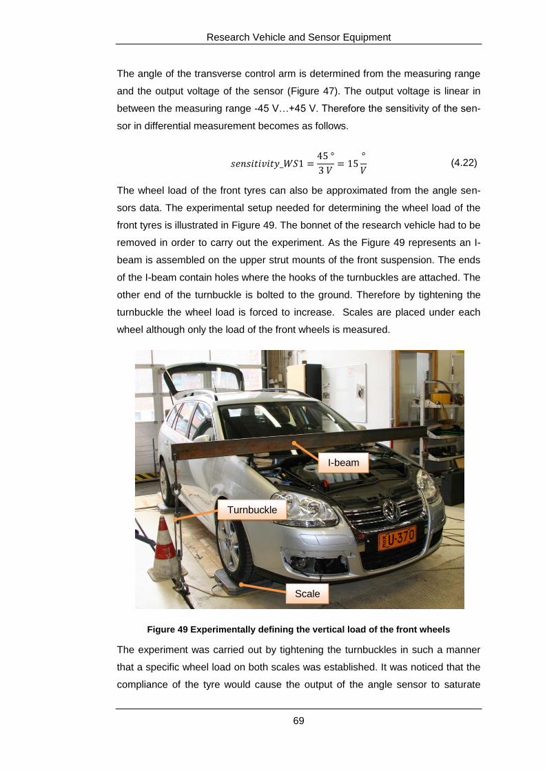
Research Vehicle and Sensor Equipment
69
The angle of the transverse control arm is determined from the measuring range
and the output voltage of the sensor (Figure 47). The output voltage is linear in
between the measuring range -45 V…+45 V. Therefore the sensitivity of the sen-
sor in differential measurement becomes as follows.
(4.22)
The wheel load of the front tyres can also be approximated from the angle sen-
sors data. The experimental setup needed for determining the wheel load of the
front tyres is illustrated in Figure 49. The bonnet of the research vehicle had to be
removed in order to carry out the experiment. As the Figure 49 represents an I-
beam is assembled on the upper strut mounts of the front suspension. The ends
of the I-beam contain holes where the hooks of the turnbuckles are attached. The
other end of the turnbuckle is bolted to the ground. Therefore by tightening the
turnbuckle the wheel load is forced to increase. Scales are placed under each
wheel although only the load of the front wheels is measured.
Figure 49 Experimentally defining the vertical load of the front wheels
The experiment was carried out by tightening the turnbuckles in such a manner
that a specific wheel load on both scales was established. It was noticed that the
compliance of the tyre would cause the output of the angle sensor to saturate
Scale
Turnbuckle
I-beam
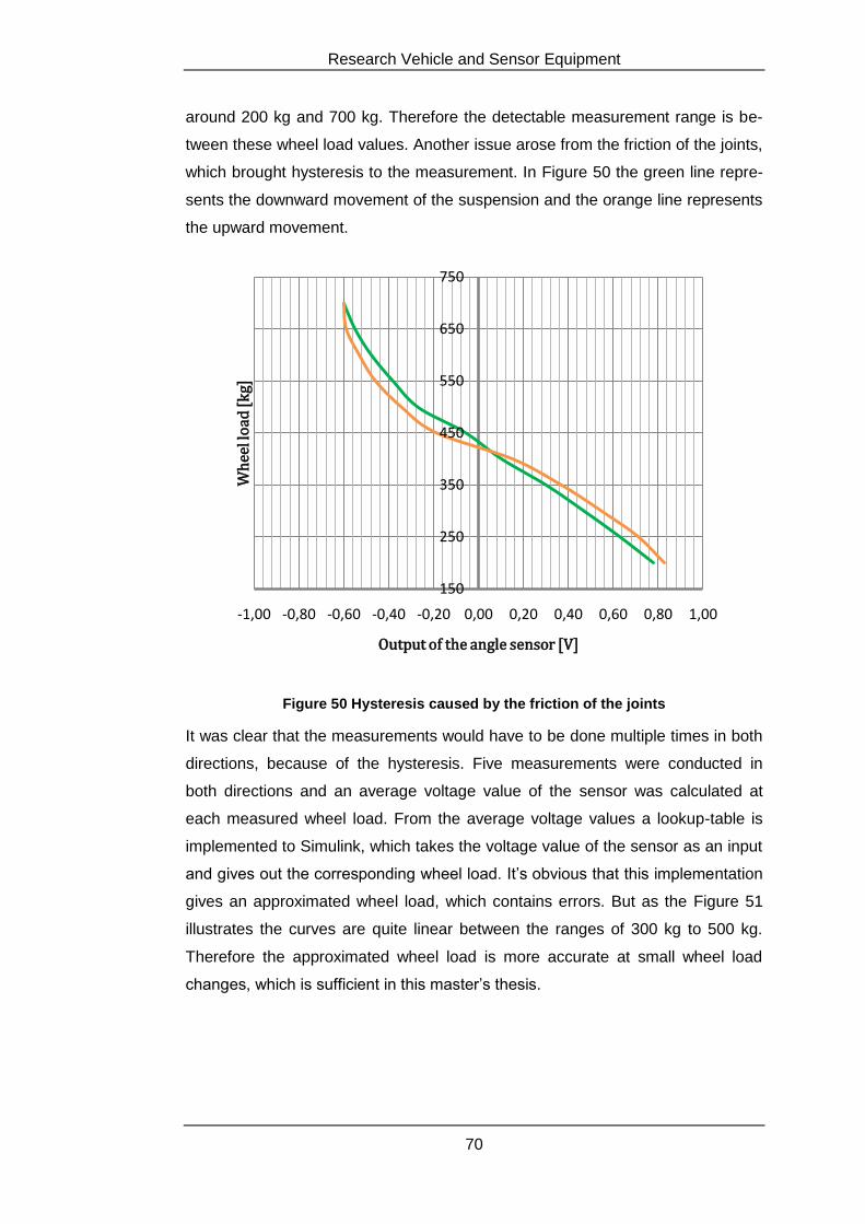
Research Vehicle and Sensor Equipment
70
around 200 kg and 700 kg. Therefore the detectable measurement range is be-
tween these wheel load values. Another issue arose from the friction of the joints,
which brought hysteresis to the measurement. In Figure 50 the green line repre-
sents the downward movement of the suspension and the orange line represents
the upward movement.
Figure 50 Hysteresis caused by the friction of the joints
It was clear that the measurements would have to be done multiple times in both
directions, because of the hysteresis. Five measurements were conducted in
both directions and an average voltage value of the sensor was calculated at
each measured wheel load. From the average voltage values a lookup-table is
implemented to Simulink, which takes the voltage value of the sensor as an input
and gives out the corresponding wheel load. It’s obvious that this implementation
gives an approximated wheel load, which contains errors. But as the Figure 51
illustrates the curves are quite linear between the ranges of 300 kg to 500 kg.
Therefore the approximated wheel load is more accurate at small wheel load
changes, which is sufficient in this master’s thesis.
150
250
350
450
550
650
750
-1,00 -0,80 -0,60 -0,40 -0,20 0,00 0,20 0,40 0,60 0,80 1,00
Wh
eel l
oad
[k
g]
Output of the angle sensor [V]
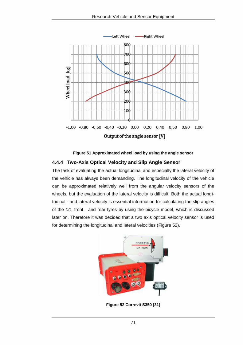
Research Vehicle and Sensor Equipment
71
Figure 51 Approximated wheel load by using the angle sensor
4.4.4 Two-Axis Optical Velocity and Slip Angle Sensor
The task of evaluating the actual longitudinal and especially the lateral velocity of
the vehicle has always been demanding. The longitudinal velocity of the vehicle
can be approximated relatively well from the angular velocity sensors of the
wheels, but the evaluation of the lateral velocity is difficult. Both the actual longi-
tudinal - and lateral velocity is essential information for calculating the slip angles
of the , front - and rear tyres by using the bicycle model, which is discussed
later on. Therefore it was decided that a two axis optical velocity sensor is used
for determining the longitudinal and lateral velocities (Figure 52).
Figure 52 Correvit S350 [31]
0
100
200
300
400
500
600
700
800
-1,00 -0,80 -0,60 -0,40 -0,20 0,00 0,20 0,40 0,60 0,80 1,00
Wh
eel l
oad
[k
g]
Output of the angle sensor [V]
Left Wheel Right Wheel
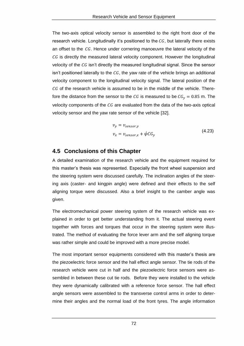
Research Vehicle and Sensor Equipment
72
The two-axis optical velocity sensor is assembled to the right front door of the
research vehicle. Longitudinally it’s positioned to the , but laterally there exists
an offset to the . Hence under cornering manoeuvre the lateral velocity of the
is directly the measured lateral velocity component. However the longitudinal
velocity of the isn’t directly the measured longitudinal signal. Since the sensor
isn’t positioned laterally to the , the yaw rate of the vehicle brings an additional
velocity component to the longitudinal velocity signal. The lateral position of the
of the research vehicle is assumed to be in the middle of the vehicle. There-
fore the distance from the sensor to the is measured to be m. The
velocity components of the are evaluated from the data of the two-axis optical
velocity sensor and the yaw rate sensor of the vehicle [32].
(4.23)
4.5 Conclusions of this Chapter
A detailed examination of the research vehicle and the equipment required for
this master’s thesis was represented. Especially the front wheel suspension and
the steering system were discussed carefully. The inclination angles of the steer-
ing axis (caster- and kingpin angle) were defined and their effects to the self
aligning torque were discussed. Also a brief insight to the camber angle was
given.
The electromechanical power steering system of the research vehicle was ex-
plained in order to get better understanding from it. The actual steering event
together with forces and torques that occur in the steering system were illus-
trated. The method of evaluating the force lever arm and the self aligning torque
was rather simple and could be improved with a more precise model.
The most important sensor equipments considered with this master’s thesis are
the piezoelectric force sensor and the hall effect angle sensor. The tie rods of the
research vehicle were cut in half and the piezoelectric force sensors were as-
sembled in between these cut tie rods. Before they were installed to the vehicle
they were dynamically calibrated with a reference force sensor. The hall effect
angle sensors were assembled to the transverse control arms in order to deter-
mine their angles and the normal load of the front tyres. The angle information
Research Vehicle and Sensor Equipment
73
was also utilised to define the caster - and kingpin inclination angles of the steer-
ing axis. The compliance of the tyre defined the detectable measuring range of
the normal load to be around 200…700 kg.
The two axis velocity - and slip angle sensor was used for attaining the real ve-
locities in longitudinal and especially in lateral direction. Also it provided the op-
portunity to evaluate the axle-specific slip angles and obviously the slip angle of
the vehicle.
Proving Grounds and Experimental Tests
74
5 Proving Grounds and Experimental Tests
5.1 Introduction
For evaluating the operation of the friction estimation method, different road sur-
face conditions are needed. A brief investigation of the proving grounds near the
capital area showed that there isn’t any single track, which could provide both
high - and low friction circumstances for conducting steady-state cornering ma-
noeuvres. Thus two different proving grounds are chosen for performing the ex-
perimental tests.
The first experimental tests are performed at the Nokian Tyres plc proving
ground, which is located in Finland at the town of Nokia. The proving ground of
Nokian Tyres plc provides the circumstances for conducting steady-state corner-
ing manoeuvres on a typical Finnish road surface, which has high micro- and
macro-texture qualities. The second experimental tests are performed at the test
driving track of Uudenmaan Ajoharjoitteluradat plc, which is also located in
Finland at the town of Vantaa. The road surface of the test driving track of Uu-
denmaan Ajoharjoitteluradat plc is divided to three lanes. The inner- and outer-
most lanes of the circle are constructed from asphalt, which has almost similar
properties as the road surface of the circle in Nokia. The middle lane on the other
hand is constructed from a special type concrete, which provides extreme slip-
pery conditions. The three different types of experimental tests conducted at the
test driving track of Uudenmaan Ajoharjoitteluradat are explained thoroughly in
this chapter.
5.2 Proving Ground of Nokian Tyres
5.2.1 Overview
Figure 53 illustrates a view from the proving ground of Nokian Tyres plc. The
main objective of this work is to estimate the friction state of the front tyres in
steady-state cornering manoeuvre. The circle (number 2 in Figure 53) of the
proving ground of Nokian Tyres provides perfect circumstances for conducting
these manoeuvres on a typical Finnish road surface. The radius of the circle is
around 40 m and it contains also a system, which can make the surface wet.
Therefore tests both in dry - and wet conditions are performed.
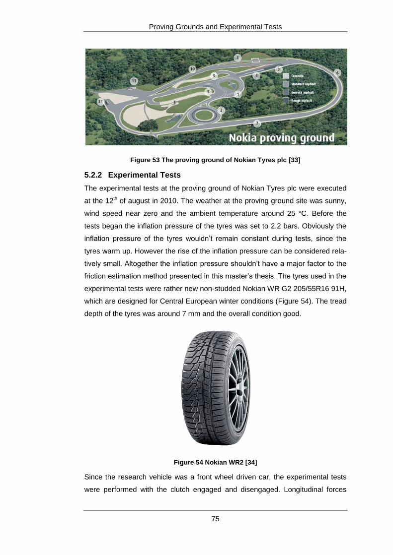
Proving Grounds and Experimental Tests
75
Figure 53 The proving ground of Nokian Tyres plc [33]
5.2.2 Experimental Tests
The experimental tests at the proving ground of Nokian Tyres plc were executed
at the 12th of august in 2010. The weather at the proving ground site was sunny,
wind speed near zero and the ambient temperature around 25 C. Before the
tests began the inflation pressure of the tyres was set to 2.2 bars. Obviously the
inflation pressure of the tyres wouldn’t remain constant during tests, since the
tyres warm up. However the rise of the inflation pressure can be considered rela-
tively small. Altogether the inflation pressure shouldn’t have a major factor to the
friction estimation method presented in this master’s thesis. The tyres used in the
experimental tests were rather new non-studded Nokian WR G2 205/55R16 91H,
which are designed for Central European winter conditions (Figure 54). The tread
depth of the tyres was around 7 mm and the overall condition good.
Figure 54 Nokian WR2 [34]
Since the research vehicle was a front wheel driven car, the experimental tests
were performed with the clutch engaged and disengaged. Longitudinal forces
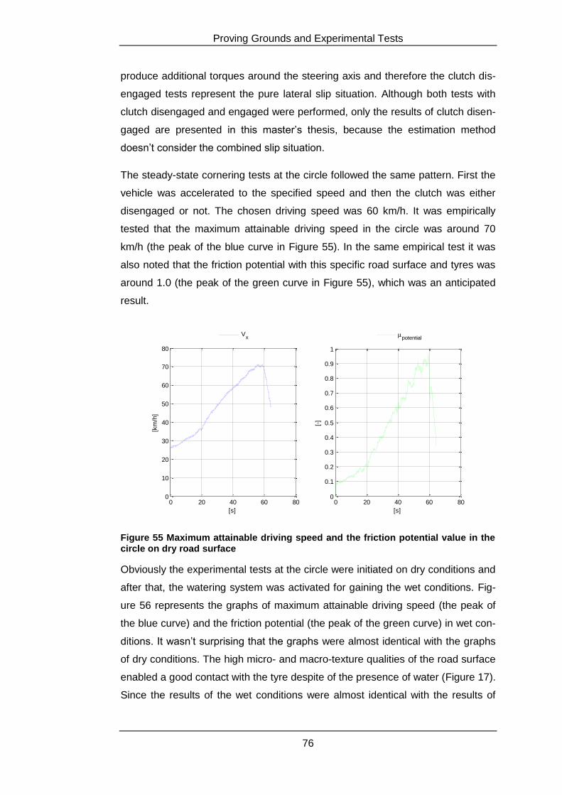
Proving Grounds and Experimental Tests
76
produce additional torques around the steering axis and therefore the clutch dis-
engaged tests represent the pure lateral slip situation. Although both tests with
clutch disengaged and engaged were performed, only the results of clutch disen-
gaged are presented in this master’s thesis, because the estimation method
doesn’t consider the combined slip situation.
The steady-state cornering tests at the circle followed the same pattern. First the
vehicle was accelerated to the specified speed and then the clutch was either
disengaged or not. The chosen driving speed was 60 km/h. It was empirically
tested that the maximum attainable driving speed in the circle was around 70
km/h (the peak of the blue curve in Figure 55). In the same empirical test it was
also noted that the friction potential with this specific road surface and tyres was
around 1.0 (the peak of the green curve in Figure 55), which was an anticipated
result.
Figure 55 Maximum attainable driving speed and the friction potential value in the circle on dry road surface
Obviously the experimental tests at the circle were initiated on dry conditions and
after that, the watering system was activated for gaining the wet conditions. Fig-
ure 56 represents the graphs of maximum attainable driving speed (the peak of
the blue curve) and the friction potential (the peak of the green curve) in wet con-
ditions. It wasn’t surprising that the graphs were almost identical with the graphs
of dry conditions. The high micro- and macro-texture qualities of the road surface
enabled a good contact with the tyre despite of the presence of water (Figure 17).
Since the results of the wet conditions were almost identical with the results of
0 20 40 60 800
10
20
30
40
50
60
70
80
[km
/h]
[s]
0 20 40 60 800
0.1
0.2
0.3
0.4
0.5
0.6
0.7
0.8
0.9
1
[-]
[s]
Vx
potential
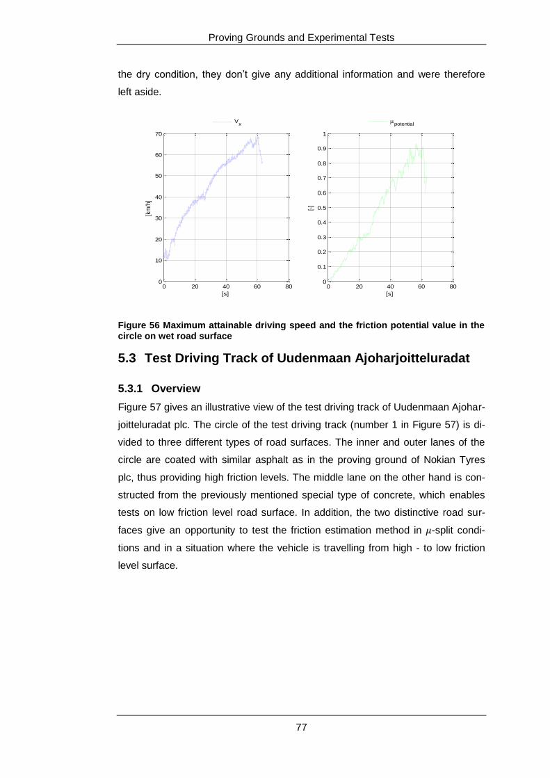
Proving Grounds and Experimental Tests
77
the dry condition, they don’t give any additional information and were therefore
left aside.
Figure 56 Maximum attainable driving speed and the friction potential value in the circle on wet road surface
5.3 Test Driving Track of Uudenmaan Ajoharjoitteluradat
5.3.1 Overview
Figure 57 gives an illustrative view of the test driving track of Uudenmaan Ajohar-
joitteluradat plc. The circle of the test driving track (number 1 in Figure 57) is di-
vided to three different types of road surfaces. The inner and outer lanes of the
circle are coated with similar asphalt as in the proving ground of Nokian Tyres
plc, thus providing high friction levels. The middle lane on the other hand is con-
structed from the previously mentioned special type of concrete, which enables
tests on low friction level road surface. In addition, the two distinctive road sur-
faces give an opportunity to test the friction estimation method in -split condi-
tions and in a situation where the vehicle is travelling from high - to low friction
level surface.
0 20 40 60 800
10
20
30
40
50
60
70
[km
/h]
[s]
Vx
0 20 40 60 800
0.1
0.2
0.3
0.4
0.5
0.6
0.7
0.8
0.9
1
[-]
[s]
potential
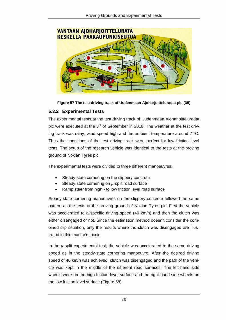
Proving Grounds and Experimental Tests
78
Figure 57 The test driving track of Uudenmaan Ajoharjoitteluradat plc [35]
5.3.2 Experimental Tests
The experimental tests at the test driving track of Uudenmaan Ajoharjoitteluradat
plc were executed at the 3rd of September in 2010. The weather at the test driv-
ing track was rainy, wind speed high and the ambient temperature around 7 C.
Thus the conditions of the test driving track were perfect for low friction level
tests. The setup of the research vehicle was identical to the tests at the proving
ground of Nokian Tyres plc.
The experimental tests were divided to three different manoeuvres:
Steady-state cornering on the slippery concrete
Steady-state cornering on -split road surface
Ramp steer from high - to low friction level road surface
Steady-state cornering manoeuvres on the slippery concrete followed the same
pattern as the tests at the proving ground of Nokian Tyres plc. First the vehicle
was accelerated to a specific driving speed (40 km/h) and then the clutch was
either disengaged or not. Since the estimation method doesn’t consider the com-
bined slip situation, only the results where the clutch was disengaged are illus-
trated in this master’s thesis.
In the -split experimental test, the vehicle was accelerated to the same driving
speed as in the steady-state cornering manoeuvre. After the desired driving
speed of 40 km/h was achieved, clutch was disengaged and the path of the vehi-
cle was kept in the middle of the different road surfaces. The left-hand side
wheels were on the high friction level surface and the right-hand side wheels on
the low friction level surface (Figure 58).
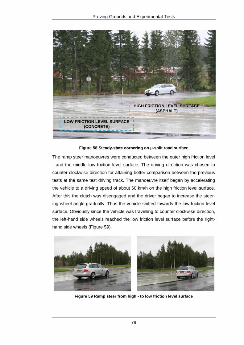
Proving Grounds and Experimental Tests
79
Figure 58 Steady-state cornering on μ-split road surface
The ramp steer manoeuvres were conducted between the outer high friction level
- and the middle low friction level surface. The driving direction was chosen to
counter clockwise direction for attaining better comparison between the previous
tests at the same test driving track. The manoeuvre itself began by accelerating
the vehicle to a driving speed of about 60 km/h on the high friction level surface.
After this the clutch was disengaged and the driver began to increase the steer-
ing wheel angle gradually. Thus the vehicle shifted towards the low friction level
surface. Obviously since the vehicle was travelling to counter clockwise direction,
the left-hand side wheels reached the low friction level surface before the right-
hand side wheels (Figure 59).
Figure 59 Ramp steer from high - to low friction level surface
LOW FRICTION LEVEL SURFACE
(CONCRETE)
HIGH FRICTION LEVEL SURFACE
(ASPHALT)
Proving Grounds and Experimental Tests
80
5.4 Conclusions of this Chapter
The experimental tests were implemented on two distinctive proving grounds.
The first experimental tests were performed at the proving ground of Nokian
Tyres plc. It provided the circumstances for testing the estimation method in typi-
cal Finnish road surface conditions. Steady-state cornering tests both in dry and -
wet conditions were executed. However since the road surface and the tyres pro-
vided good grip also in the wet conditions, no difference compared to the dry
conditions were observed. Therefore the results of the wet conditions were left
aside of this master’s thesis. The second experimental tests were conducted at
the test driving track of Uudenmaan Ajoharjoitteluradat plc. It provided the cir-
cumstances for steady-state cornering tests on low friction level road surface.
The circle at the test driving track of Uudenmaan Ajoharjoitteluradat plc was con-
structed of three different lanes. The inner - and outer lanes were coated with
asphalt and the middle lane with slippery concrete. Therefore it provided the op-
portunity for trying out the estimation method in -split conditions and in situation
where the vehicle was travelling from high friction surface to low friction level sur-
face.
Friction Estimation Method
81
6 Friction Estimation Method
6.1 Introduction
Chapter 4 introduced the required equipment and input signals for the friction
estimation. This chapter explains how the required input signals are exploited in
order to derive the complete friction state of the tyre. To start with the models of
the vehicle and the tyre are introduced.
The planar motion of the vehicle is modelled with the well-known single track
model, which provides the axle specific lateral force - and slip angle information
[1]. Literature is also familiar with the brush tyre model, which explains the force
generation of a tyre under lateral -, longitudinal - or combined slip situations [36].
Only the pure lateral slip situation is examined here, since the friction estimation
introduced in this master’s thesis assumes a pure cornering manoeuvre.
However the brush tyre model isn’t used to derive the forces and torques of the
tyre, but they are given to it as inputs. This provides an opportunity to exploit the
brush tyre model for estimating friction potential, - used and - available. The es-
timation principle together with the requirements and limitations are given in the
last subchapter. A proof of concept is also represented.
6.2 The Bicycle Model
6.2.1 Definition and Assumptions
There has to be a mathematical model of the actual vehicle for analysing its pla-
nar motion and handling characteristics. The bicycle model is in many cases a
sufficient tool for studying the handling of a vehicle. Since the bicycle model sim-
plifies the actual vehicle in many ways, there are several assumptions and re-
quirements that have to be taken into consideration. The assumptions and re-
quirements are listed below:
No lateral load transfer [1]
No longitudinal load transfer [1]
No rolling or pitching motions [1]
No chassis or suspension compliance effects [1]
Tyres have the same slip angle on the same axle [1]
Steering wheel angle and slip angles are small [1]
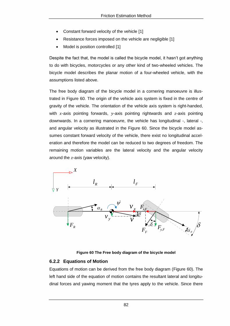
Friction Estimation Method
82
Constant forward velocity of the vehicle [1]
Resistance forces imposed on the vehicle are negligible [1]
Model is position controlled [1]
Despite the fact that, the model is called the bicycle model, it hasn’t got anything
to do with bicycles, motorcycles or any other kind of two-wheeled vehicles. The
bicycle model describes the planar motion of a four-wheeled vehicle, with the
assumptions listed above.
The free body diagram of the bicycle model in a cornering manoeuvre is illus-
trated in Figure 60. The origin of the vehicle axis system is fixed in the centre of
gravity of the vehicle. The orientation of the vehicle axis system is right-handed,
with -axis pointing forwards, -axis pointing rightwards and -axis pointing
downwards. In a cornering manoeuvre, the vehicle has longitudinal -, lateral -,
and angular velocity as illustrated in the Figure 60. Since the bicycle model as-
sumes constant forward velocity of the vehicle, there exist no longitudinal accel-
eration and therefore the model can be reduced to two degrees of freedom. The
remaining motion variables are the lateral velocity and the angular velocity
around the -axis (yaw velocity).
xv
yv
F
R
FlRl
v
Y
FyF ,
FFRF
FxF ,
X
Figure 60 The Free body diagram of the bicycle model
6.2.2 Equations of Motion
Equations of motion can be derived from the free body diagram (Figure 60). The
left hand side of the equation of motion contains the resultant lateral and longitu-
dinal forces and yawing moment that the tyres apply to the vehicle. Since there
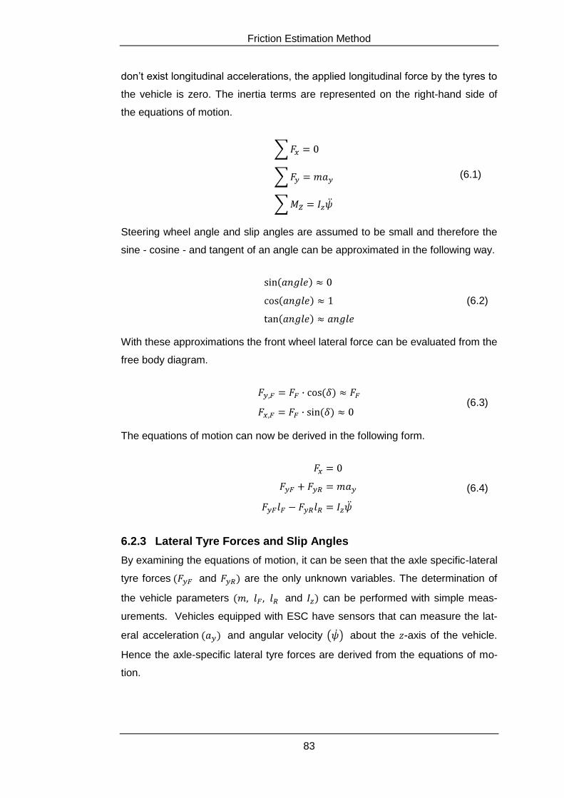
Friction Estimation Method
83
don’t exist longitudinal accelerations, the applied longitudinal force by the tyres to
the vehicle is zero. The inertia terms are represented on the right-hand side of
the equations of motion.
(6.1)
Steering wheel angle and slip angles are assumed to be small and therefore the
sine - cosine - and tangent of an angle can be approximated in the following way.
(6.2)
With these approximations the front wheel lateral force can be evaluated from the
free body diagram.
(6.3)
The equations of motion can now be derived in the following form.
(6.4)
6.2.3 Lateral Tyre Forces and Slip Angles
By examining the equations of motion, it can be seen that the axle specific-lateral
tyre forces and are the only unknown variables. The determination of
the vehicle parameters and can be performed with simple meas-
urements. Vehicles equipped with ESC have sensors that can measure the lat-
eral acceleration and angular velocity about the -axis of the vehicle.
Hence the axle-specific lateral tyre forces are derived from the equations of mo-
tion.
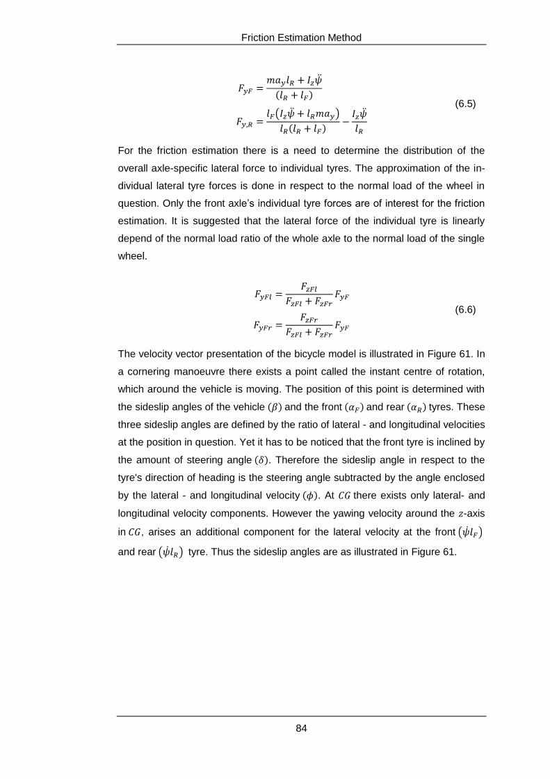
Friction Estimation Method
84
(6.5)
For the friction estimation there is a need to determine the distribution of the
overall axle-specific lateral force to individual tyres. The approximation of the in-
dividual lateral tyre forces is done in respect to the normal load of the wheel in
question. Only the front axle’s individual tyre forces are of interest for the friction
estimation. It is suggested that the lateral force of the individual tyre is linearly
depend of the normal load ratio of the whole axle to the normal load of the single
wheel.
(6.6)
The velocity vector presentation of the bicycle model is illustrated in Figure 61. In
a cornering manoeuvre there exists a point called the instant centre of rotation,
which around the vehicle is moving. The position of this point is determined with
the sideslip angles of the vehicle and the front and rear tyres. These
three sideslip angles are defined by the ratio of lateral - and longitudinal velocities
at the position in question. Yet it has to be noticed that the front tyre is inclined by
the amount of steering angle . Therefore the sideslip angle in respect to the
tyre's direction of heading is the steering angle subtracted by the angle enclosed
by the lateral - and longitudinal velocity . At there exists only lateral- and
longitudinal velocity components. However the yawing velocity around the -axis
in , arises an additional component for the lateral velocity at the front
and rear tyre. Thus the sideslip angles are as illustrated in Figure 61.
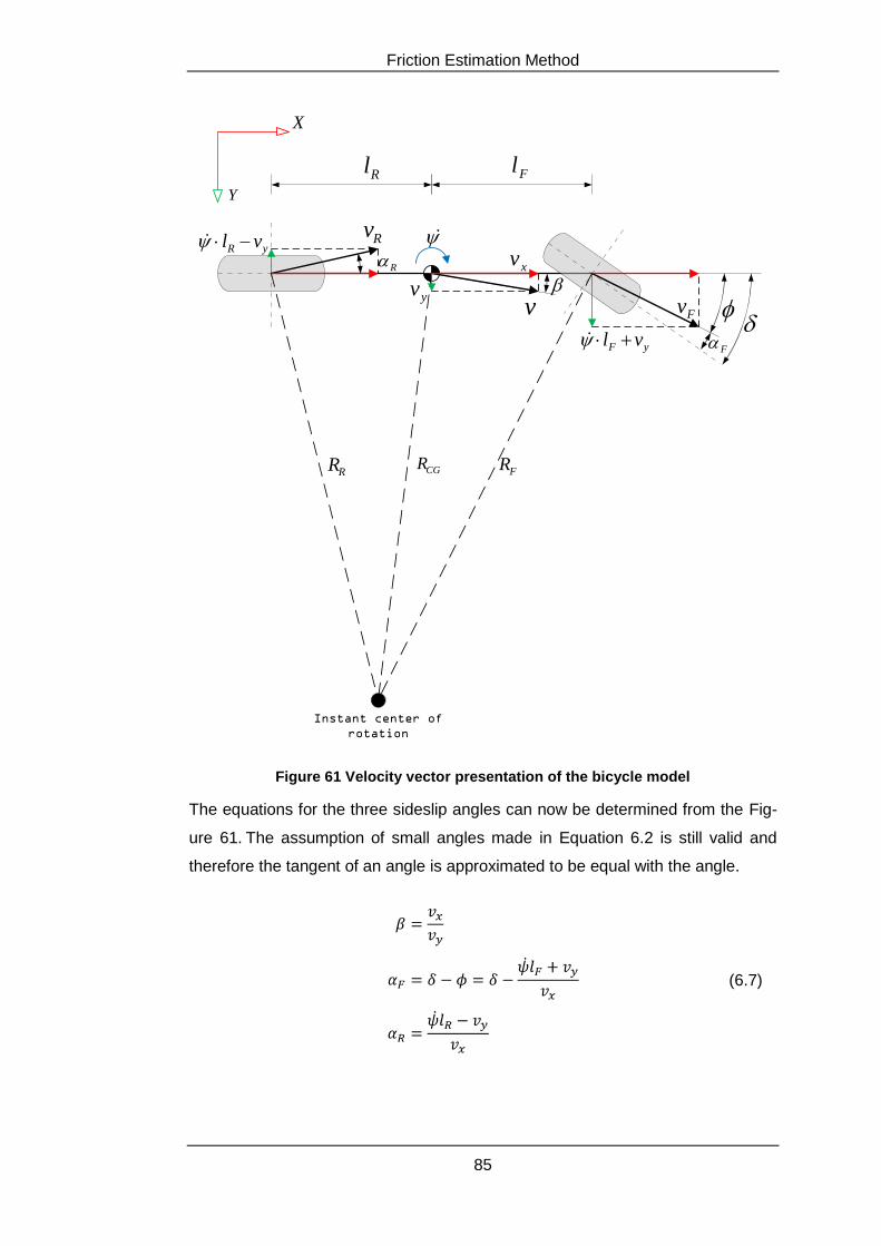
Friction Estimation Method
85
xv
yv
F
R
X
FRRR
FlRl
v
CGR
yR vl
yF vl
Y
Instant center of
rotation
Rv
Fv
Figure 61 Velocity vector presentation of the bicycle model
The equations for the three sideslip angles can now be determined from the Fig-
ure 61. The assumption of small angles made in Equation 6.2 is still valid and
therefore the tangent of an angle is approximated to be equal with the angle.
(6.7)
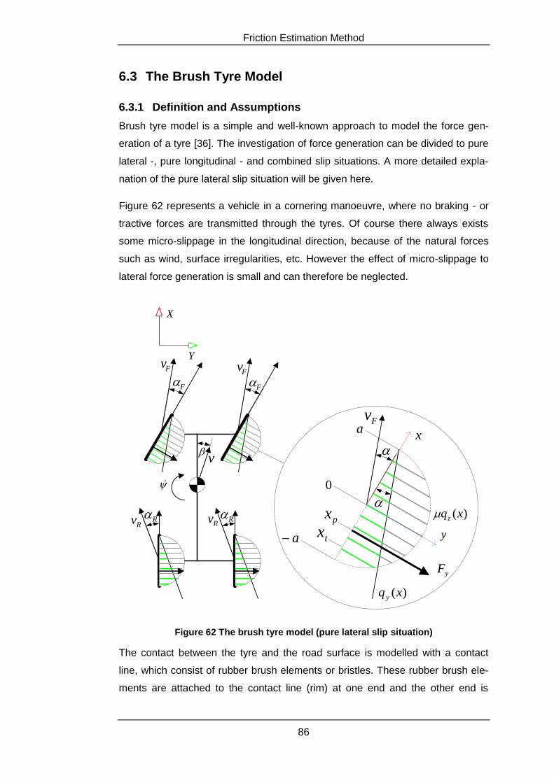
Friction Estimation Method
86
6.3 The Brush Tyre Model
6.3.1 Definition and Assumptions
Brush tyre model is a simple and well-known approach to model the force gen-
eration of a tyre [36]. The investigation of force generation can be divided to pure
lateral -, pure longitudinal - and combined slip situations. A more detailed expla-
nation of the pure lateral slip situation will be given here.
Figure 62 represents a vehicle in a cornering manoeuvre, where no braking - or
tractive forces are transmitted through the tyres. Of course there always exists
some micro-slippage in the longitudinal direction, because of the natural forces
such as wind, surface irregularities, etc. However the effect of micro-slippage to
lateral force generation is small and can therefore be neglected.
F
Rv
X
Y
R
a
yF
a txpx
0
Fv
x
)(xqz
)(xq y
y
F
R
Fv
v
Fv
Rv
Figure 62 The brush tyre model (pure lateral slip situation)
The contact between the tyre and the road surface is modelled with a contact
line, which consist of rubber brush elements or bristles. These rubber brush ele-
ments are attached to the contact line (rim) at one end and the other end is
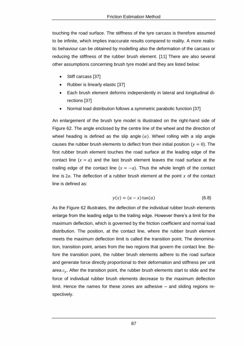
Friction Estimation Method
87
touching the road surface. The stiffness of the tyre carcass is therefore assumed
to be infinite, which implies inaccurate results compared to reality. A more realis-
tic behaviour can be obtained by modelling also the deformation of the carcass or
reducing the stiffness of the rubber brush element. [11] There are also several
other assumptions concerning brush tyre model and they are listed below:
Stiff carcass [37]
Rubber is linearly elastic [37]
Each brush element deforms independently in lateral and longitudinal di-
rections [37]
Normal load distribution follows a symmetric parabolic function [37]
An enlargement of the brush tyre model is illustrated on the right-hand side of
Figure 62. The angle enclosed by the centre line of the wheel and the direction of
wheel heading is defined as the slip angle . Wheel rolling with a slip angle
causes the rubber brush elements to deflect from their initial position ( ). The
first rubber brush element touches the road surface at the leading edge of the
contact line ( ) and the last brush element leaves the road surface at the
trailing edge of the contact line ( ). Thus the whole length of the contact
line is . The deflection of a rubber brush element at the point of the contact
line is defined as:
(6.8)
As the Figure 62 illustrates, the deflection of the individual rubber brush elements
enlarge from the leading edge to the trailing edge. However there’s a limit for the
maximum deflection, which is governed by the friction coefficient and normal load
distribution. The position, at the contact line, where the rubber brush element
meets the maximum deflection limit is called the transition point. The denomina-
tion, transition point, arises from the two regions that govern the contact line. Be-
fore the transition point, the rubber brush elements adhere to the road surface
and generate force directly proportional to their deformation and stiffness per unit
area . After the transition point, the rubber brush elements start to slide and the
force of individual rubber brush elements decrease to the maximum deflection
limit. Hence the names for these zones are adhesive – and sliding regions re-
spectively.
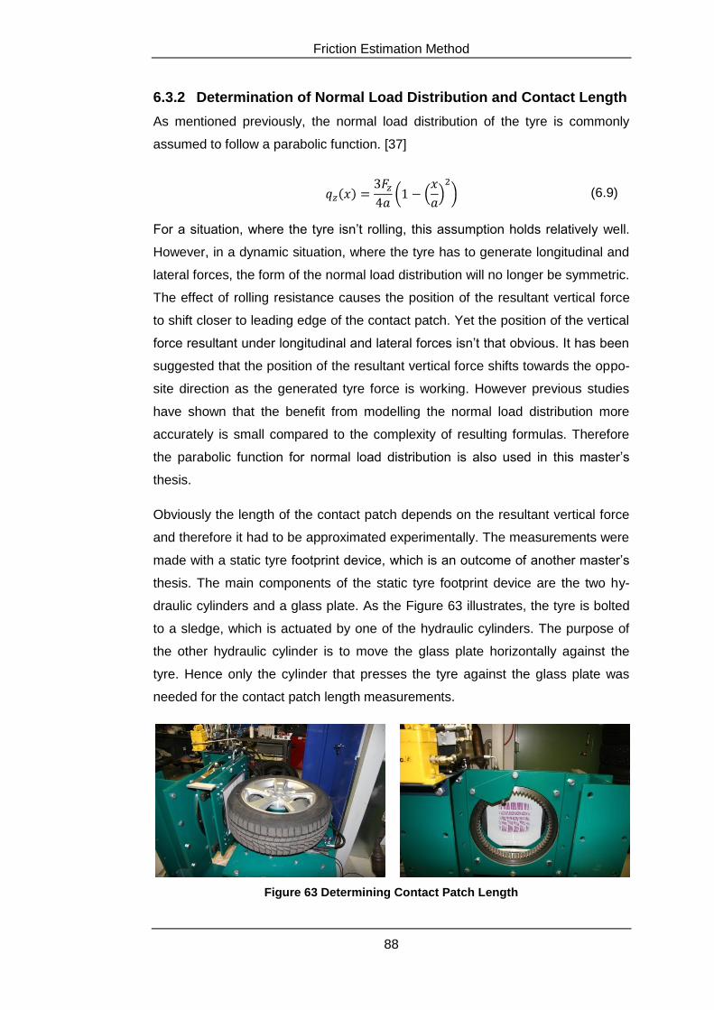
Friction Estimation Method
88
6.3.2 Determination of Normal Load Distribution and Contact Length
As mentioned previously, the normal load distribution of the tyre is commonly
assumed to follow a parabolic function. [37]
(6.9)
For a situation, where the tyre isn’t rolling, this assumption holds relatively well.
However, in a dynamic situation, where the tyre has to generate longitudinal and
lateral forces, the form of the normal load distribution will no longer be symmetric.
The effect of rolling resistance causes the position of the resultant vertical force
to shift closer to leading edge of the contact patch. Yet the position of the vertical
force resultant under longitudinal and lateral forces isn’t that obvious. It has been
suggested that the position of the resultant vertical force shifts towards the oppo-
site direction as the generated tyre force is working. However previous studies
have shown that the benefit from modelling the normal load distribution more
accurately is small compared to the complexity of resulting formulas. Therefore
the parabolic function for normal load distribution is also used in this master’s
thesis.
Obviously the length of the contact patch depends on the resultant vertical force
and therefore it had to be approximated experimentally. The measurements were
made with a static tyre footprint device, which is an outcome of another master’s
thesis. The main components of the static tyre footprint device are the two hy-
draulic cylinders and a glass plate. As the Figure 63 illustrates, the tyre is bolted
to a sledge, which is actuated by one of the hydraulic cylinders. The purpose of
the other hydraulic cylinder is to move the glass plate horizontally against the
tyre. Hence only the cylinder that presses the tyre against the glass plate was
needed for the contact patch length measurements.
Figure 63 Determining Contact Patch Length
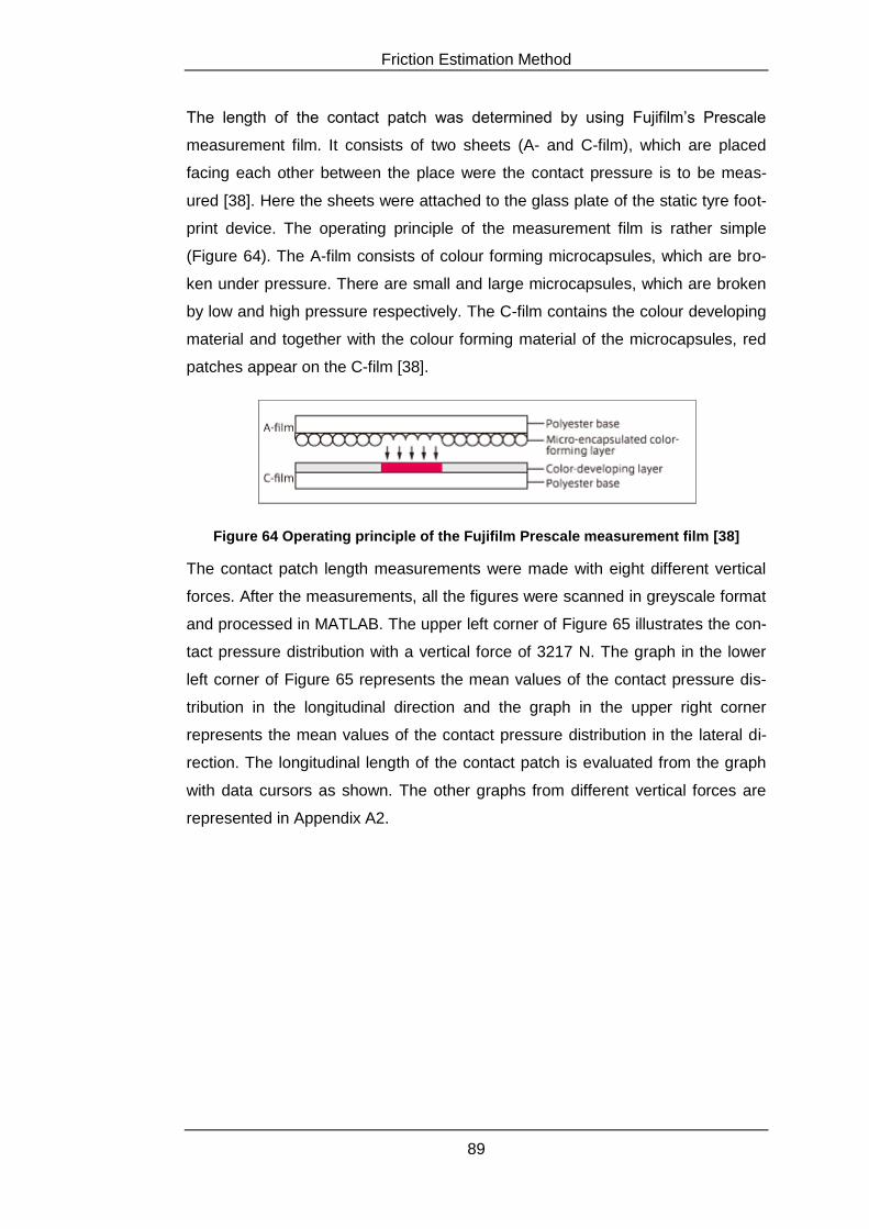
Friction Estimation Method
89
The length of the contact patch was determined by using Fujifilm’s Prescale
measurement film. It consists of two sheets (A- and C-film), which are placed
facing each other between the place were the contact pressure is to be meas-
ured [38]. Here the sheets were attached to the glass plate of the static tyre foot-
print device. The operating principle of the measurement film is rather simple
(Figure 64). The A-film consists of colour forming microcapsules, which are bro-
ken under pressure. There are small and large microcapsules, which are broken
by low and high pressure respectively. The C-film contains the colour developing
material and together with the colour forming material of the microcapsules, red
patches appear on the C-film [38].
Figure 64 Operating principle of the Fujifilm Prescale measurement film [38]
The contact patch length measurements were made with eight different vertical
forces. After the measurements, all the figures were scanned in greyscale format
and processed in MATLAB. The upper left corner of Figure 65 illustrates the con-
tact pressure distribution with a vertical force of 3217 N. The graph in the lower
left corner of Figure 65 represents the mean values of the contact pressure dis-
tribution in the longitudinal direction and the graph in the upper right corner
represents the mean values of the contact pressure distribution in the lateral di-
rection. The longitudinal length of the contact patch is evaluated from the graph
with data cursors as shown. The other graphs from different vertical forces are
represented in Appendix A2.
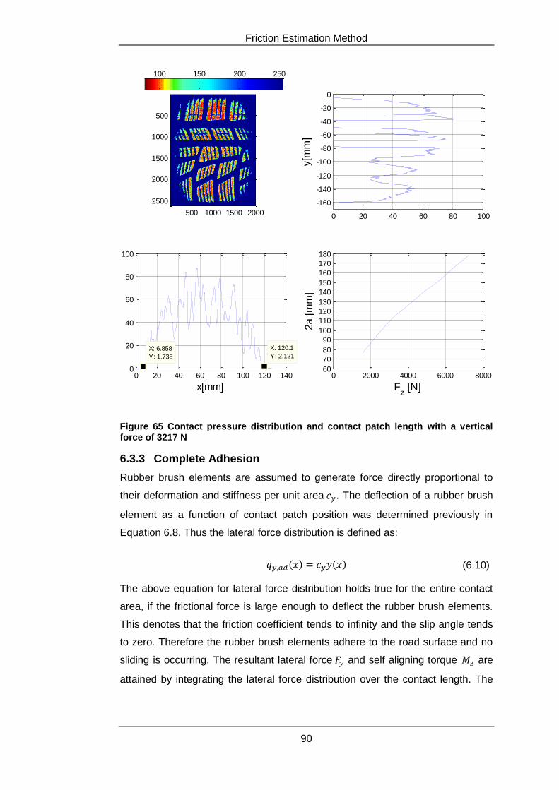
Friction Estimation Method
90
Figure 65 Contact pressure distribution and contact patch length with a vertical force of 3217 N
6.3.3 Complete Adhesion
Rubber brush elements are assumed to generate force directly proportional to
their deformation and stiffness per unit area . The deflection of a rubber brush
element as a function of contact patch position was determined previously in
Equation 6.8. Thus the lateral force distribution is defined as:
(6.10)
The above equation for lateral force distribution holds true for the entire contact
area, if the frictional force is large enough to deflect the rubber brush elements.
This denotes that the friction coefficient tends to infinity and the slip angle tends
to zero. Therefore the rubber brush elements adhere to the road surface and no
sliding is occurring. The resultant lateral force and self aligning torque are
attained by integrating the lateral force distribution over the contact length. The
500 1000 1500 2000
500
1000
1500
2000
2500
0 20 40 60 80 100 120 1400
20
40
60
80
100
X: 120.1
Y: 2.121
x[mm]
X: 6.858
Y: 1.738
0 20 40 60 80 100
-160
-140
-120
-100
-80
-60
-40
-20
0
y[m
m]
0 2000 4000 6000 800060
70
80
90
100
110
120
130
140
150
160
170
180
Fz [N]
2a
[m
m]
100 150 200 250
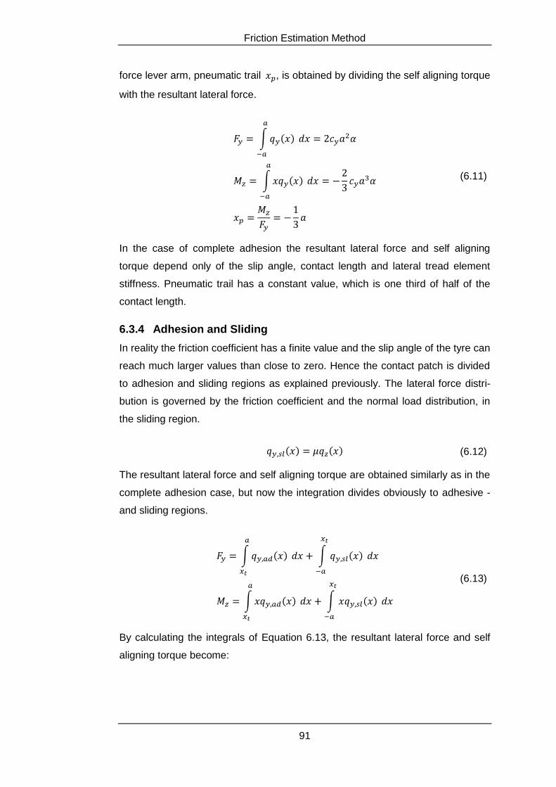
Friction Estimation Method
91
force lever arm, pneumatic trail , is obtained by dividing the self aligning torque
with the resultant lateral force.
(6.11)
In the case of complete adhesion the resultant lateral force and self aligning
torque depend only of the slip angle, contact length and lateral tread element
stiffness. Pneumatic trail has a constant value, which is one third of half of the
contact length.
6.3.4 Adhesion and Sliding
In reality the friction coefficient has a finite value and the slip angle of the tyre can
reach much larger values than close to zero. Hence the contact patch is divided
to adhesion and sliding regions as explained previously. The lateral force distri-
bution is governed by the friction coefficient and the normal load distribution, in
the sliding region.
(6.12)
The resultant lateral force and self aligning torque are obtained similarly as in the
complete adhesion case, but now the integration divides obviously to adhesive -
and sliding regions.
(6.13)
By calculating the integrals of Equation 6.13, the resultant lateral force and self
aligning torque become:
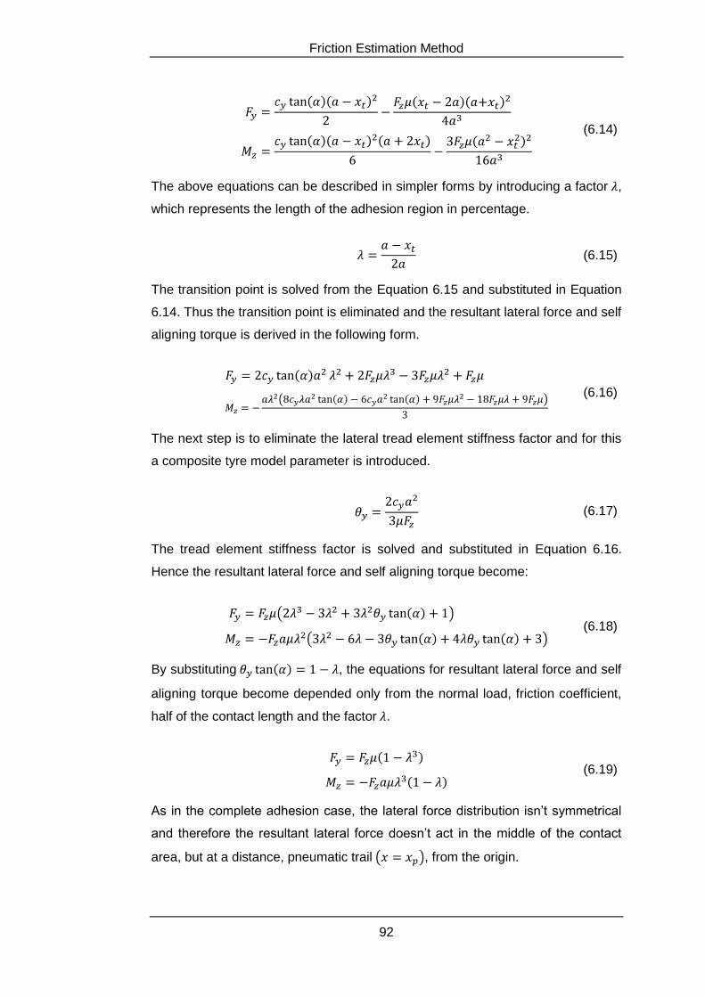
Friction Estimation Method
92
(6.14)
The above equations can be described in simpler forms by introducing a factor ,
which represents the length of the adhesion region in percentage.
(6.15)
The transition point is solved from the Equation 6.15 and substituted in Equation
6.14. Thus the transition point is eliminated and the resultant lateral force and self
aligning torque is derived in the following form.
(6.16)
The next step is to eliminate the lateral tread element stiffness factor and for this
a composite tyre model parameter is introduced.
(6.17)
The tread element stiffness factor is solved and substituted in Equation 6.16.
Hence the resultant lateral force and self aligning torque become:
(6.18)
By substituting , the equations for resultant lateral force and self
aligning torque become depended only from the normal load, friction coefficient,
half of the contact length and the factor .
(6.19)
As in the complete adhesion case, the lateral force distribution isn’t symmetrical
and therefore the resultant lateral force doesn’t act in the middle of the contact
area, but at a distance, pneumatic trail , from the origin.
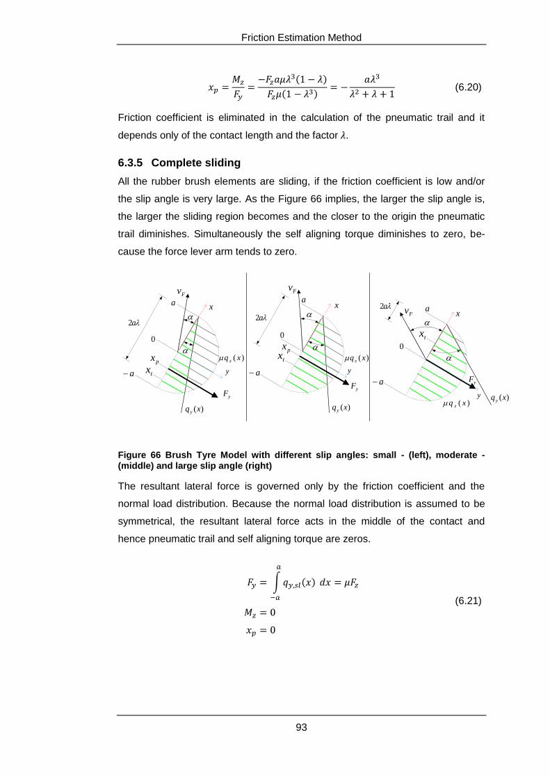
Friction Estimation Method
93
(6.20)
Friction coefficient is eliminated in the calculation of the pneumatic trail and it
depends only of the contact length and the factor .
6.3.5 Complete sliding
All the rubber brush elements are sliding, if the friction coefficient is low and/or
the slip angle is very large. As the Figure 66 implies, the larger the slip angle is,
the larger the sliding region becomes and the closer to the origin the pneumatic
trail diminishes. Simultaneously the self aligning torque diminishes to zero, be-
cause the force lever arm tends to zero.
a
yF
a txpx
0
Fv
x
)( xq z
)(xq y
y
a2a2
a2
a
0
0px
tx
aa
)(xq z
y
yF
)(xq y
x
a
yF
y )(xq y)( xq z
tx
x
Fv
Fv
Figure 66 Brush Tyre Model with different slip angles: small - (left), moderate - (middle) and large slip angle (right)
The resultant lateral force is governed only by the friction coefficient and the
normal load distribution. Because the normal load distribution is assumed to be
symmetrical, the resultant lateral force acts in the middle of the contact and
hence pneumatic trail and self aligning torque are zeros.
(6.21)
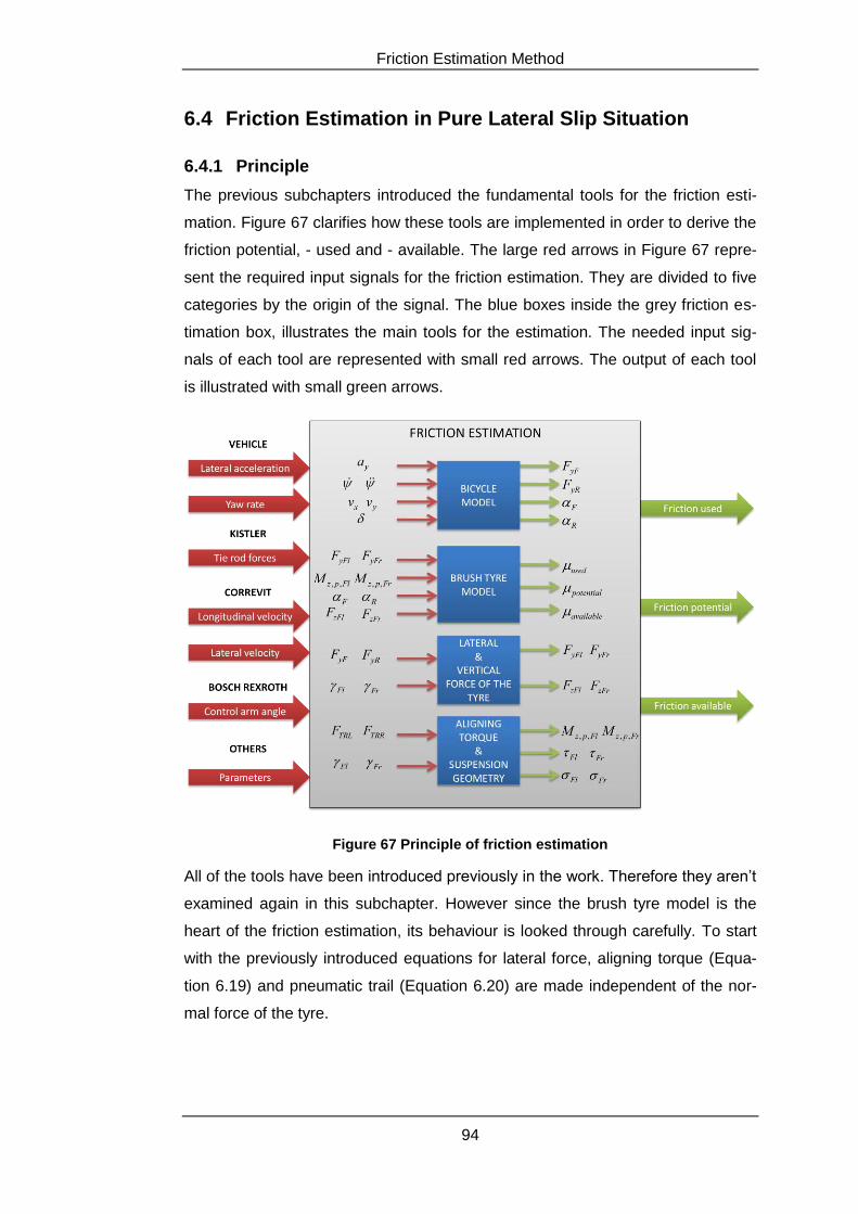
Friction Estimation Method
94
6.4 Friction Estimation in Pure Lateral Slip Situation
6.4.1 Principle
The previous subchapters introduced the fundamental tools for the friction esti-
mation. Figure 67 clarifies how these tools are implemented in order to derive the
friction potential, - used and - available. The large red arrows in Figure 67 repre-
sent the required input signals for the friction estimation. They are divided to five
categories by the origin of the signal. The blue boxes inside the grey friction es-
timation box, illustrates the main tools for the estimation. The needed input sig-
nals of each tool are represented with small red arrows. The output of each tool
is illustrated with small green arrows.
Figure 67 Principle of friction estimation
All of the tools have been introduced previously in the work. Therefore they aren’t
examined again in this subchapter. However since the brush tyre model is the
heart of the friction estimation, its behaviour is looked through carefully. To start
with the previously introduced equations for lateral force, aligning torque (Equa-
tion 6.19) and pneumatic trail (Equation 6.20) are made independent of the nor-
mal force of the tyre.
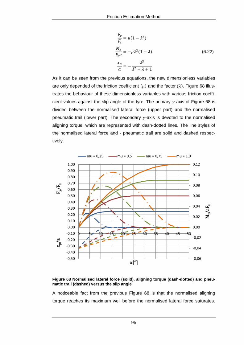
Friction Estimation Method
95
(6.22)
As it can be seen from the previous equations, the new dimensionless variables
are only depended of the friction coefficient and the factor . Figure 68 illus-
trates the behaviour of these dimensionless variables with various friction coeffi-
cient values against the slip angle of the tyre. The primary -axis of Figure 68 is
divided between the normalised lateral force (upper part) and the normalised
pneumatic trail (lower part). The secondary -axis is devoted to the normalised
aligning torque, which are represented with dash-dotted lines. The line styles of
the normalised lateral force and - pneumatic trail are solid and dashed respec-
tively.
Figure 68 Normalised lateral force (solid), aligning torque (dash-dotted) and pneu-matic trail (dashed) versus the slip angle
A noticeable fact from the previous Figure 68 is that the normalised aligning
torque reaches its maximum well before the normalised lateral force saturates.
-0,06
-0,04
-0,02
0,00
0,02
0,04
0,06
0,08
0,10
0,12
-0,50
-0,40
-0,30
-0,20
-0,10
0,00
0,10
0,20
0,30
0,40
0,50
0,60
0,70
0,80
0,90
1,00
0 5 10 15 20 25 30 35 40 45 50
Mz/
aFz
Fy/
F z
α[°]
mu = 0,25 mu = 0,5 mu = 0,75 mu = 1,0
x p/a

Friction Estimation Method
96
Therefore the normalised aligning torque provides a possibility to estimate friction
potential before the tyre is totally sliding. On the other hand when the tyre is to-
tally sliding, both the normalised pneumatic trail and the aligning torque tends to
zero, which hinders the use of aligning torque to friction estimation. The sensitiv-
ity of the normalised lateral force and - aligning torque are discussed in the next
subchapter.
By observing the previously derived equations of normalised lateral force, - align-
ing torque and - pneumatic trail (Equation 6.22), it’s noticed that there are three
equations and only two unknown variables. This provides a possibility to evaluate
the friction potential separately as a function of normalised lateral force and -
aligning torque. Equation 6.23 represents the friction potential as function of the
normalised lateral force and the factor .
(6.23)
The friction potential derived from the normalised aligning torque is represented
in Equation 6.24.
(6.24)
Both of the previous equations contain also the other unknown variable, which is
the factor . One approach of solving the factor would be placing the previ-
ous equations equal, but the result is a 3rd degree function, which doesn’t have
an unambiguous solution. However the equation of normalized pneumatic trail
can be exploited for evaluating the factor . The equation of normalised pneu-
matic trail is only depended of the factor , which signifies that a specific value
of normalised pneumatic trail corresponds to a specific value of the factor .
Therefore a look-up table can be constructed, which takes the normalised pneu-
matic trail as an input and gives out the corresponding value of factor (Table
2).
Table 2 Factor and the corresponding value of normalised pneumatic trail
λ [-]
0,00 0,10 0,20 0,30 0,40 0,50 0,60 0,70 0,80 0,90 1,00
xp / a [-]
0,0000 0,0009 0,0065 0,0194 0,0410 0,0714 0,1102 0,1566 0,2098 0,2690 0,3333
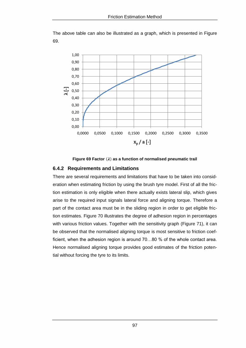
Friction Estimation Method
97
The above table can also be illustrated as a graph, which is presented in Figure
69.
Figure 69 Factor as a function of normalised pneumatic trail
6.4.2 Requirements and Limitations
There are several requirements and limitations that have to be taken into consid-
eration when estimating friction by using the brush tyre model. First of all the fric-
tion estimation is only eligible when there actually exists lateral slip, which gives
arise to the required input signals lateral force and aligning torque. Therefore a
part of the contact area must be in the sliding region in order to get eligible fric-
tion estimates. Figure 70 illustrates the degree of adhesion region in percentages
with various friction values. Together with the sensitivity graph (Figure 71), it can
be observed that the normalised aligning torque is most sensitive to friction coef-
ficient, when the adhesion region is around 70…80 % of the whole contact area.
Hence normalised aligning torque provides good estimates of the friction poten-
tial without forcing the tyre to its limits.
0,00
0,10
0,20
0,30
0,40
0,50
0,60
0,70
0,80
0,90
1,00
0,0000 0,0500 0,1000 0,1500 0,2000 0,2500 0,3000 0,3500
λ[-
]
xp / a [-]
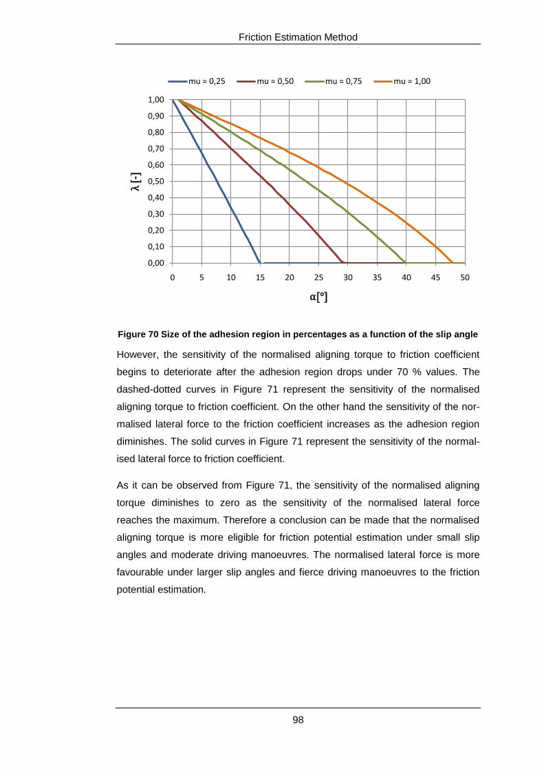
Friction Estimation Method
98
Figure 70 Size of the adhesion region in percentages as a function of the slip angle
However, the sensitivity of the normalised aligning torque to friction coefficient
begins to deteriorate after the adhesion region drops under 70 % values. The
dashed-dotted curves in Figure 71 represent the sensitivity of the normalised
aligning torque to friction coefficient. On the other hand the sensitivity of the nor-
malised lateral force to the friction coefficient increases as the adhesion region
diminishes. The solid curves in Figure 71 represent the sensitivity of the normal-
ised lateral force to friction coefficient.
As it can be observed from Figure 71, the sensitivity of the normalised aligning
torque diminishes to zero as the sensitivity of the normalised lateral force
reaches the maximum. Therefore a conclusion can be made that the normalised
aligning torque is more eligible for friction potential estimation under small slip
angles and moderate driving manoeuvres. The normalised lateral force is more
favourable under larger slip angles and fierce driving manoeuvres to the friction
potential estimation.
0,00
0,10
0,20
0,30
0,40
0,50
0,60
0,70
0,80
0,90
1,00
0 5 10 15 20 25 30 35 40 45 50
λ[-
]
α[°]
mu = 0,25 mu = 0,50 mu = 0,75 mu = 1,00
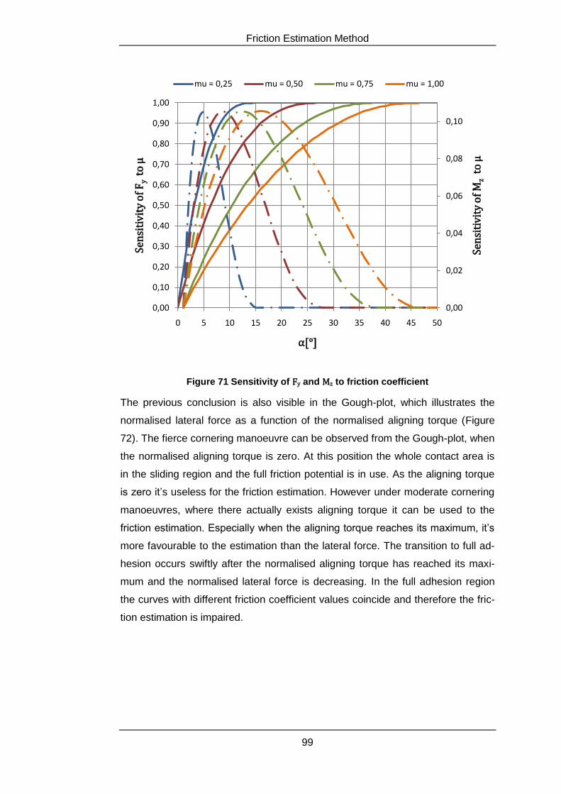
Friction Estimation Method
99
Figure 71 Sensitivity of Fy and Mz to friction coefficient
The previous conclusion is also visible in the Gough-plot, which illustrates the
normalised lateral force as a function of the normalised aligning torque (Figure
72). The fierce cornering manoeuvre can be observed from the Gough-plot, when
the normalised aligning torque is zero. At this position the whole contact area is
in the sliding region and the full friction potential is in use. As the aligning torque
is zero it’s useless for the friction estimation. However under moderate cornering
manoeuvres, where there actually exists aligning torque it can be used to the
friction estimation. Especially when the aligning torque reaches its maximum, it’s
more favourable to the estimation than the lateral force. The transition to full ad-
hesion occurs swiftly after the normalised aligning torque has reached its maxi-
mum and the normalised lateral force is decreasing. In the full adhesion region
the curves with different friction coefficient values coincide and therefore the fric-
tion estimation is impaired.
0,00
0,02
0,04
0,06
0,08
0,10
0,00
0,10
0,20
0,30
0,40
0,50
0,60
0,70
0,80
0,90
1,00
0 5 10 15 20 25 30 35 40 45 50
Sen
siti
vity
of M
zto
µ
Sen
siti
vity
of F
y to
µ
α[°]
mu = 0,25 mu = 0,50 mu = 0,75 mu = 1,00
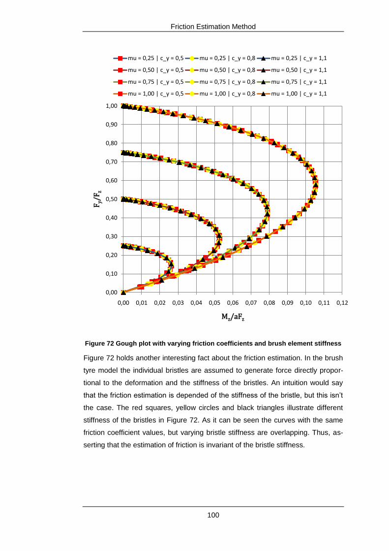
Friction Estimation Method
100
Figure 72 Gough plot with varying friction coefficients and brush element stiffness
Figure 72 holds another interesting fact about the friction estimation. In the brush
tyre model the individual bristles are assumed to generate force directly propor-
tional to the deformation and the stiffness of the bristles. An intuition would say
that the friction estimation is depended of the stiffness of the bristle, but this isn’t
the case. The red squares, yellow circles and black triangles illustrate different
stiffness of the bristles in Figure 72. As it can be seen the curves with the same
friction coefficient values, but varying bristle stiffness are overlapping. Thus, as-
serting that the estimation of friction is invariant of the bristle stiffness.
0,00
0,10
0,20
0,30
0,40
0,50
0,60
0,70
0,80
0,90
1,00
0,00 0,01 0,02 0,03 0,04 0,05 0,06 0,07 0,08 0,09 0,10 0,11 0,12
Fy/
F z
Mz/aFz
mu = 0,25 | c_y = 0,5 mu = 0,25 | c_y = 0,8 mu = 0,25 | c_y = 1,1
mu = 0,50 | c_y = 0,5 mu = 0,50 | c_y = 0,8 mu = 0,50 | c_y = 1,1
mu = 0,75 | c_y = 0,5 mu = 0,75 | c_y = 0,8 mu = 0,75 | c_y = 1,1
mu = 1,00 | c_y = 0,5 mu = 1,00 | c_y = 0,8 mu = 1,00 | c_y = 1,1
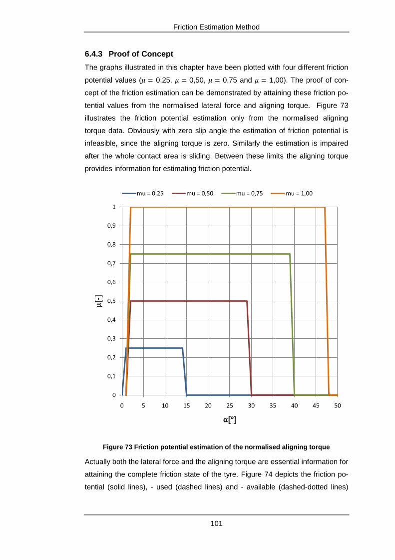
Friction Estimation Method
101
6.4.3 Proof of Concept
The graphs illustrated in this chapter have been plotted with four different friction
potential values ( 0,25, 0,50, 0,75 and 1,00). The proof of con-
cept of the friction estimation can be demonstrated by attaining these friction po-
tential values from the normalised lateral force and aligning torque. Figure 73
illustrates the friction potential estimation only from the normalised aligning
torque data. Obviously with zero slip angle the estimation of friction potential is
infeasible, since the aligning torque is zero. Similarly the estimation is impaired
after the whole contact area is sliding. Between these limits the aligning torque
provides information for estimating friction potential.
Figure 73 Friction potential estimation of the normalised aligning torque
Actually both the lateral force and the aligning torque are essential information for
attaining the complete friction state of the tyre. Figure 74 depicts the friction po-
tential (solid lines), - used (dashed lines) and - available (dashed-dotted lines)
0
0,1
0,2
0,3
0,4
0,5
0,6
0,7
0,8
0,9
1
0 5 10 15 20 25 30 35 40 45 50
µ[-
]
α[°]
mu = 0,25 mu = 0,50 mu = 0,75 mu = 1,00
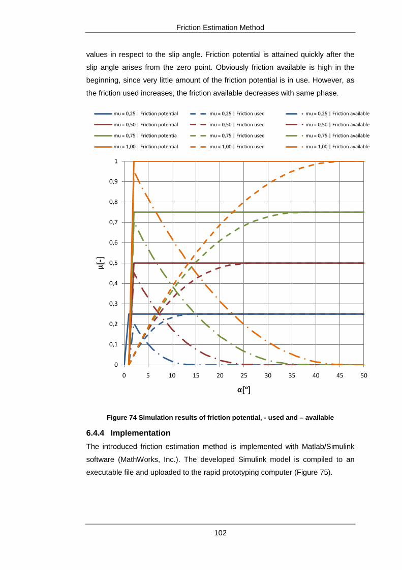
Friction Estimation Method
102
values in respect to the slip angle. Friction potential is attained quickly after the
slip angle arises from the zero point. Obviously friction available is high in the
beginning, since very little amount of the friction potential is in use. However, as
the friction used increases, the friction available decreases with same phase.
Figure 74 Simulation results of friction potential, - used and – available
6.4.4 Implementation
The introduced friction estimation method is implemented with Matlab/Simulink
software (MathWorks, Inc.). The developed Simulink model is compiled to an
executable file and uploaded to the rapid prototyping computer (Figure 75).
0
0,1
0,2
0,3
0,4
0,5
0,6
0,7
0,8
0,9
1
0 5 10 15 20 25 30 35 40 45 50
µ[-
]
α[°]
mu = 0,25 | Friction potential mu = 0,25 | Friction used mu = 0,25 | Friction available
mu = 0,50 | Friction potential mu = 0,50 | Friction used mu = 0,50 | Friction available
mu = 0,75 | Friction potentia mu = 0,75 | Friction used mu = 0,75 | Friction available
mu = 1,00 | Friction potential mu = 1,00 | Friction used mu = 1,00 | Friction available
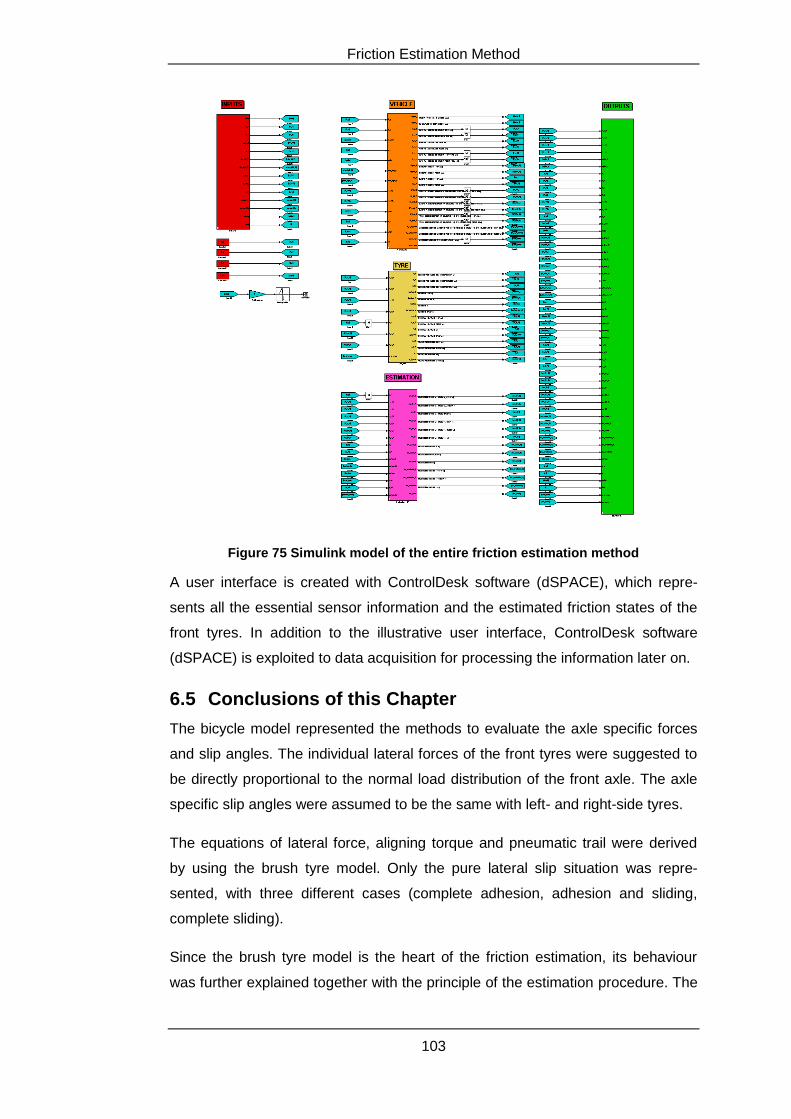
Friction Estimation Method
103
Figure 75 Simulink model of the entire friction estimation method
A user interface is created with ControlDesk software (dSPACE), which repre-
sents all the essential sensor information and the estimated friction states of the
front tyres. In addition to the illustrative user interface, ControlDesk software
(dSPACE) is exploited to data acquisition for processing the information later on.
6.5 Conclusions of this Chapter
The bicycle model represented the methods to evaluate the axle specific forces
and slip angles. The individual lateral forces of the front tyres were suggested to
be directly proportional to the normal load distribution of the front axle. The axle
specific slip angles were assumed to be the same with left- and right-side tyres.
The equations of lateral force, aligning torque and pneumatic trail were derived
by using the brush tyre model. Only the pure lateral slip situation was repre-
sented, with three different cases (complete adhesion, adhesion and sliding,
complete sliding).
Since the brush tyre model is the heart of the friction estimation, its behaviour
was further explained together with the principle of the estimation procedure. The
Friction Estimation Method
104
equations of lateral force, aligning torque and pneumatic trail were made inde-
pendent of load. These three equations provided an opportunity to solve the fric-
tion potential as a function of the normalised lateral force or the - aligning torque.
The sensitivity of the normalised lateral force and - aligning torque to friction coef-
ficient was investigated with various different friction coefficient values. A conclu-
sion was drawn that the normalised aligning torque is most sensitive to friction
coefficient, when the size of the adhesion region is around 70…80 % of the
whole contact area. Therefore providing feasible conditions for friction estimation
without, forcing the tyre to its limits. The sensitivity of the normalised lateral force
to the friction coefficient was found to increase as the adhesion region diminished
to zero. The effects of different brush element stiffness to the friction estimation
were investigated. It was noted that the friction estimation is invariant to varying
brush element stiffness.
The proof of concept from simple simulated data illustrated that the friction esti-
mation by using the brush tyre model is feasible.
Proving Ground Results and Discussion
105
7 Proving Ground Results and Discussion
7.1 Introduction
The proving grounds and the experimental tests were presented thoroughly in
Chapter 5. The purpose of this chapter is to illustrate the results from these ex-
perimental tests and discuss about them.
As described in Chapter 5, two distinctive proving grounds are used for investi-
gating the operation of the friction estimation method. The proving ground of
Nokian Tyres plc provided the circumstances for conducting steady-state corner-
ing manoeuvres on high friction level surface. The second experimental tests
were performed at the test driving track of Uudenmaan Ajoharjoitteluradat plc.
The circle at the test driving track of Uudenmaan Ajoharjoitteluradat gave an op-
portunity to three distinguished test manoeuvres, which were explained thor-
oughly in Chapter 5.
For clarification purposes, the blue curves of the graphs presented in this chapter
denote always to the properties of the left-hand side wheel and the red curves to
the properties of the right-hand side wheel. The green coloured curves, which
appear in the brush tyre model graphs, represent the averages of the left- and
right-hand side curves.
7.2 Steady-State Cornering
7.2.1 High Friction Level Road Surface
The steady-state cornering manoeuvres on high friction level road surface were
performed at the proving ground of Nokian Tyres plc. Measurements were re-
peated several times to both counter clockwise - and clockwise directions. How-
ever since the results were almost identical to both directions, only the results of
the clockwise direction are presented here.
The sensor data of the vehicle and the optical velocity sensor are illustrated in
Figure 76. As it can be seen, first the vehicle was accelerated to a driving speed
of about 55 km/h and then the clutch was disengaged at 1.516 s. Obviously
from this point forward the vehicle started to decelerate, which is also visible in
the lateral acceleration graph ( ) and the longitudinal velocity graph ( ). The
aspiration was to keep the radius of the steady-state cornering manoeuvre at a
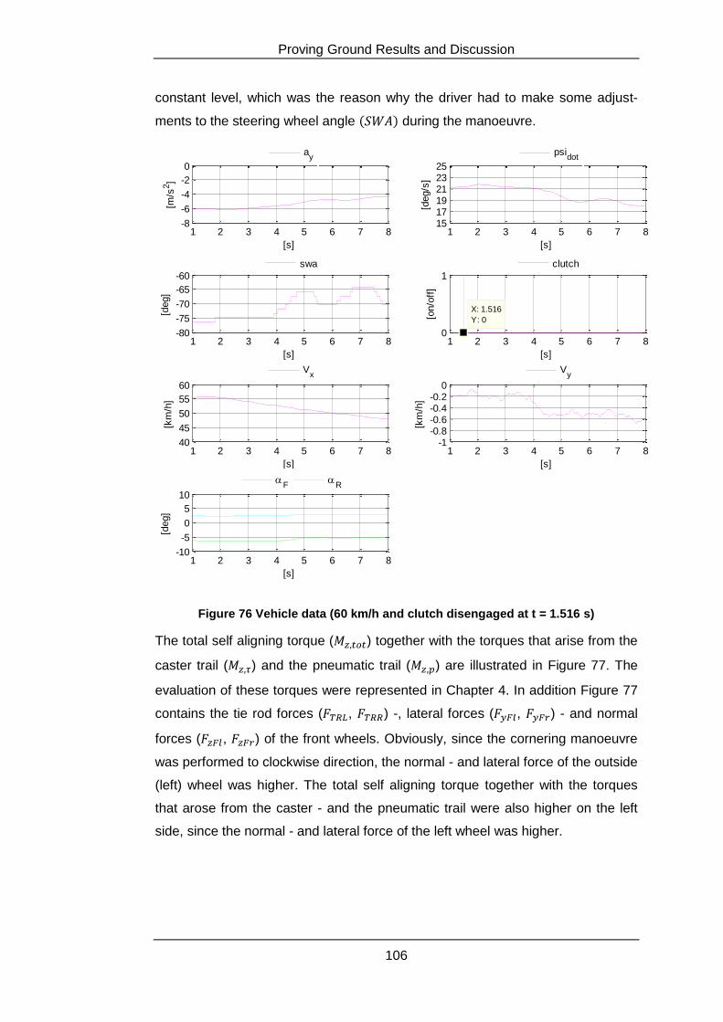
Proving Ground Results and Discussion
106
constant level, which was the reason why the driver had to make some adjust-
ments to the steering wheel angle during the manoeuvre.
Figure 76 Vehicle data (60 km/h and clutch disengaged at t = 1.516 s)
The total self aligning torque ( ) together with the torques that arise from the
caster trail ( ) and the pneumatic trail ( ) are illustrated in Figure 77. The
evaluation of these torques were represented in Chapter 4. In addition Figure 77
contains the tie rod forces ( , ) -, lateral forces ( , ) - and normal
forces ( , ) of the front wheels. Obviously, since the cornering manoeuvre
was performed to clockwise direction, the normal - and lateral force of the outside
(left) wheel was higher. The total self aligning torque together with the torques
that arose from the caster - and the pneumatic trail were also higher on the left
side, since the normal - and lateral force of the left wheel was higher.
1 2 3 4 5 6 7 8-8
-6
-4
-2
0[m
/s2]
[s]
ay
1 2 3 4 5 6 7 8151719212325
[deg/s
]
[s]
psidot
1 2 3 4 5 6 7 8-80
-75
-70
-65
-60
[deg]
[s]
swa
1 2 3 4 5 6 7 80
1
X: 1.516
Y: 0[on/o
ff]
[s]
clutch
1 2 3 4 5 6 7 840
45
50
55
60
[km
/h]
[s]
Vx
1 2 3 4 5 6 7 8-1
-0.8-0.6-0.4-0.2
0
[km
/h]
[s]
Vy
1 2 3 4 5 6 7 8-10
-5
0
5
10
[deg]
[s]
F
R
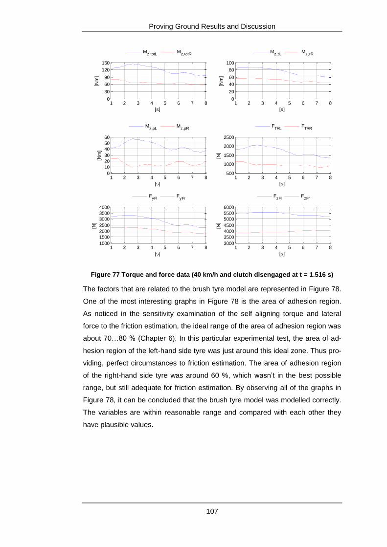
Proving Ground Results and Discussion
107
Figure 77 Torque and force data (40 km/h and clutch disengaged at t = 1.516 s)
The factors that are related to the brush tyre model are represented in Figure 78.
One of the most interesting graphs in Figure 78 is the area of adhesion region.
As noticed in the sensitivity examination of the self aligning torque and lateral
force to the friction estimation, the ideal range of the area of adhesion region was
about 70…80 % (Chapter 6). In this particular experimental test, the area of ad-
hesion region of the left-hand side tyre was just around this ideal zone. Thus pro-
viding, perfect circumstances to friction estimation. The area of adhesion region
of the right-hand side tyre was around 60 %, which wasn’t in the best possible
range, but still adequate for friction estimation. By observing all of the graphs in
Figure 78, it can be concluded that the brush tyre model was modelled correctly.
The variables are within reasonable range and compared with each other they
have plausible values.
1 2 3 4 5 6 7 80
30
60
90
120
150
[Nm
]
[s]
Mz,totL
Mz,totR
1 2 3 4 5 6 7 80
20
40
60
80
100
[Nm
]
[s]
Mz,L
Mz,R
1 2 3 4 5 6 7 80
10
20
30
40
50
60
[Nm
]
[s]
Mz,pL
Mz,pR
1 2 3 4 5 6 7 8500
1000
1500
2000
2500
[N]
[s]
FTRL
FTRR
1 2 3 4 5 6 7 81000
1500
2000
2500
3000
3500
4000
[N]
[s]
FyFl
FyFr
1 2 3 4 5 6 7 83000
3500
4000
4500
5000
5500
6000
[N]
[s]
FzFl
FzFr
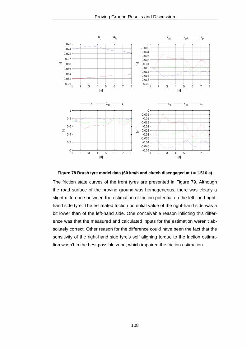
Proving Ground Results and Discussion
108
Figure 78 Brush tyre model data (60 km/h and clutch disengaged at t = 1.516 s)
The friction state curves of the front tyres are presented in Figure 79. Although
the road surface of the proving ground was homogeneous, there was clearly a
slight difference between the estimation of friction potential on the left- and right-
hand side tyre. The estimated friction potential value of the right-hand side was a
bit lower than of the left-hand side. One conceivable reason inflicting this differ-
ence was that the measured and calculated inputs for the estimation weren’t ab-
solutely correct. Other reason for the difference could have been the fact that the
sensitivity of the right-hand side tyre’s self aligning torque to the friction estima-
tion wasn’t in the best possible zone, which impaired the friction estimation.
1 2 3 4 5 6 7 80.06
0.062
0.064
0.066
0.068
0.07
0.072
0.074
0.076
[m]
[s]
aL
aR
1 2 3 4 5 6 7 8-0.02
-0.018
-0.016
-0.014
-0.012
-0.01
-0.008
-0.006
-0.004
-0.002
0
[m]
[s]
xpL
xpR
xp
1 2 3 4 5 6 7 80
0.2
0.4
0.6
0.8
1
[-]
[s]
L
R
1 2 3 4 5 6 7 8-0.05
-0.045
-0.04
-0.035
-0.03
-0.025
-0.02
-0.015
-0.01
-0.005
0
[m]
[s]
xtL
xtR
xt
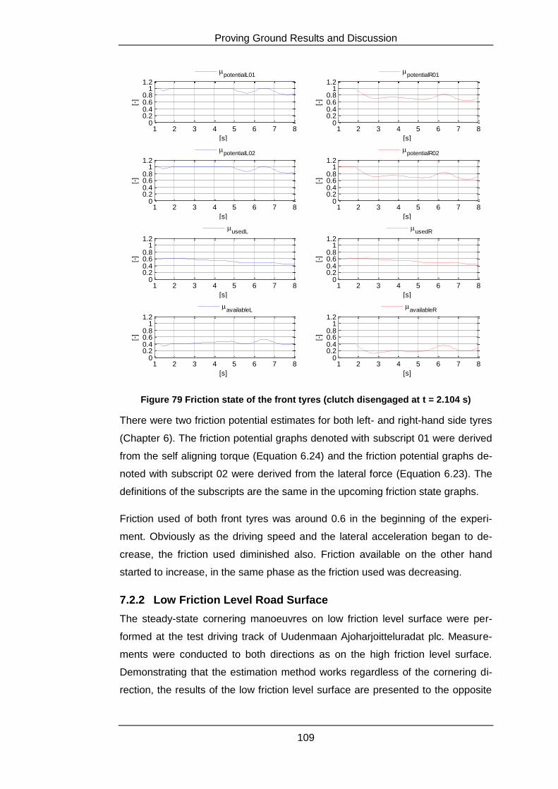
Proving Ground Results and Discussion
109
Figure 79 Friction state of the front tyres (clutch disengaged at t = 2.104 s)
There were two friction potential estimates for both left- and right-hand side tyres
(Chapter 6). The friction potential graphs denoted with subscript 01 were derived
from the self aligning torque (Equation 6.24) and the friction potential graphs de-
noted with subscript 02 were derived from the lateral force (Equation 6.23). The
definitions of the subscripts are the same in the upcoming friction state graphs.
Friction used of both front tyres was around 0.6 in the beginning of the experi-
ment. Obviously as the driving speed and the lateral acceleration began to de-
crease, the friction used diminished also. Friction available on the other hand
started to increase, in the same phase as the friction used was decreasing.
7.2.2 Low Friction Level Road Surface
The steady-state cornering manoeuvres on low friction level surface were per-
formed at the test driving track of Uudenmaan Ajoharjoitteluradat plc. Measure-
ments were conducted to both directions as on the high friction level surface.
Demonstrating that the estimation method works regardless of the cornering di-
rection, the results of the low friction level surface are presented to the opposite
1 2 3 4 5 6 7 80
0.20.40.60.8
11.2
[-]
[s]
potentialL01
1 2 3 4 5 6 7 80
0.20.40.60.8
11.2
[-]
[s]
potentialR01
1 2 3 4 5 6 7 80
0.20.40.60.8
11.2
[-]
[s]
potentialL02
1 2 3 4 5 6 7 80
0.20.40.60.8
11.2
[-]
[s]
potentialR02
1 2 3 4 5 6 7 80
0.20.40.60.8
11.2
[-]
[s]
usedL
1 2 3 4 5 6 7 80
0.20.40.60.8
11.2
[-]
[s]
usedR
1 2 3 4 5 6 7 80
0.20.40.60.8
11.2
[-]
[s]
availableL
1 2 3 4 5 6 7 80
0.20.40.60.8
11.2
[-]
[s]
availableR
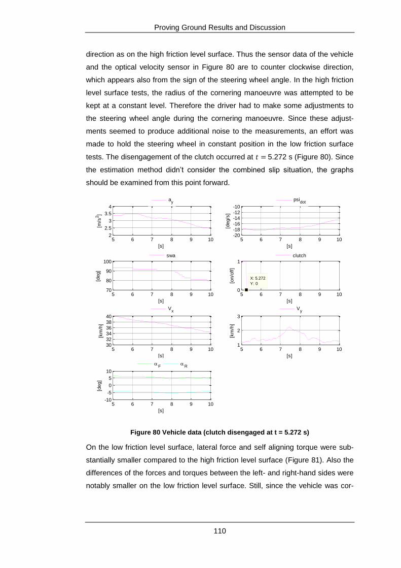
Proving Ground Results and Discussion
110
direction as on the high friction level surface. Thus the sensor data of the vehicle
and the optical velocity sensor in Figure 80 are to counter clockwise direction,
which appears also from the sign of the steering wheel angle. In the high friction
level surface tests, the radius of the cornering manoeuvre was attempted to be
kept at a constant level. Therefore the driver had to make some adjustments to
the steering wheel angle during the cornering manoeuvre. Since these adjust-
ments seemed to produce additional noise to the measurements, an effort was
made to hold the steering wheel in constant position in the low friction surface
tests. The disengagement of the clutch occurred at 5.272 s (Figure 80). Since
the estimation method didn’t consider the combined slip situation, the graphs
should be examined from this point forward.
Figure 80 Vehicle data (clutch disengaged at t = 5.272 s)
On the low friction level surface, lateral force and self aligning torque were sub-
stantially smaller compared to the high friction level surface (Figure 81). Also the
differences of the forces and torques between the left- and right-hand sides were
notably smaller on the low friction level surface. Still, since the vehicle was cor-
5 6 7 8 9 102
2.5
3
3.5
4
[m/s
2]
[s]
ay
5 6 7 8 9 10-20-18-16-14-12-10
[deg/s
]
[s]
psidot
5 6 7 8 9 1070
80
90
100
[deg]
[s]
swa
5 6 7 8 9 100
1
X: 5.272
Y: 0[on/o
ff]
[s]
clutch
5 6 7 8 9 10303234363840
[km
/h]
[s]
Vx
5 6 7 8 9 101
2
3
[km
/h]
[s]
Vy
5 6 7 8 9 10-10
-5
0
5
10
[deg]
[s]
F
R
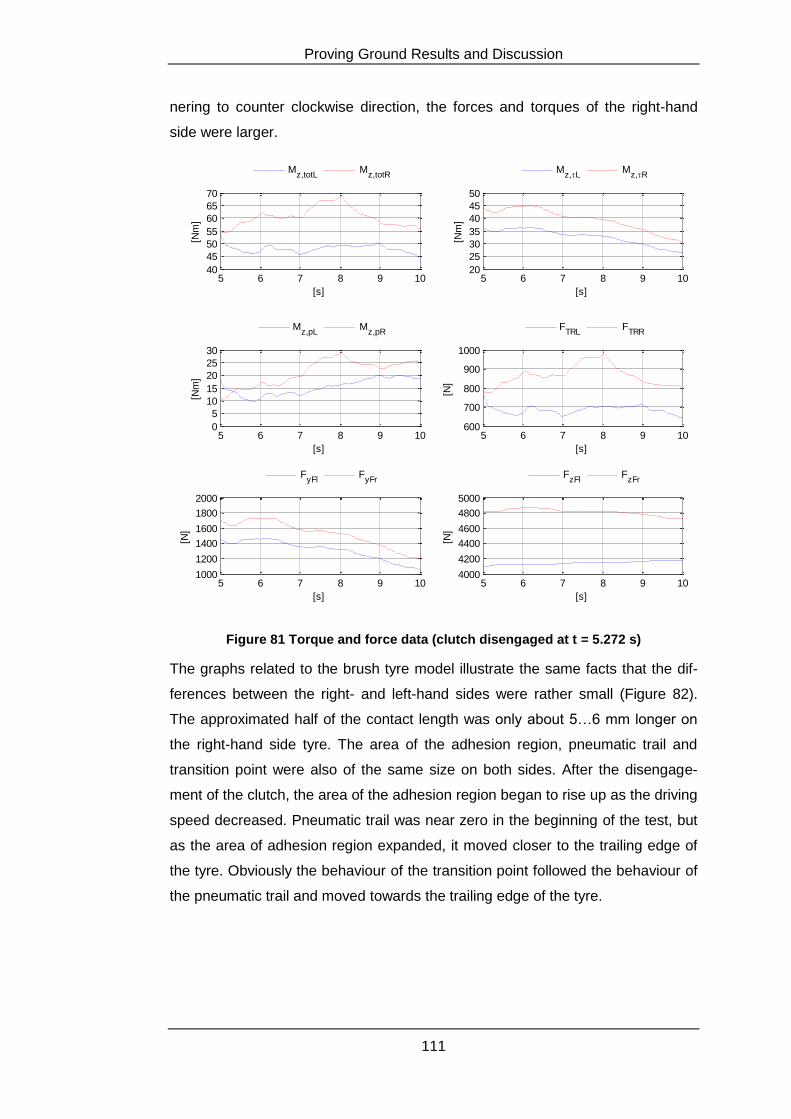
Proving Ground Results and Discussion
111
nering to counter clockwise direction, the forces and torques of the right-hand
side were larger.
Figure 81 Torque and force data (clutch disengaged at t = 5.272 s)
The graphs related to the brush tyre model illustrate the same facts that the dif-
ferences between the right- and left-hand sides were rather small (Figure 82).
The approximated half of the contact length was only about 5…6 mm longer on
the right-hand side tyre. The area of the adhesion region, pneumatic trail and
transition point were also of the same size on both sides. After the disengage-
ment of the clutch, the area of the adhesion region began to rise up as the driving
speed decreased. Pneumatic trail was near zero in the beginning of the test, but
as the area of adhesion region expanded, it moved closer to the trailing edge of
the tyre. Obviously the behaviour of the transition point followed the behaviour of
the pneumatic trail and moved towards the trailing edge of the tyre.
5 6 7 8 9 1040
45
50
55
60
65
70[N
m]
[s]
Mz,totL
Mz,totR
5 6 7 8 9 1020
25
30
35
40
45
50
[Nm
]
[s]
Mz,L
Mz,R
5 6 7 8 9 100
5
10
15
20
25
30
[Nm
]
[s]
Mz,pL
Mz,pR
5 6 7 8 9 10600
700
800
900
1000
[N]
[s]
FTRL
FTRR
5 6 7 8 9 101000
1200
1400
1600
1800
2000
[N]
[s]
FyFl
FyFr
5 6 7 8 9 104000
4200
4400
4600
4800
5000
[N]
[s]
FzFl
FzFr

Proving Ground Results and Discussion
112
Figure 82 Brush tyre model data (clutch disengaged at t = 5.272 s)
The friction states of the front tyres on the low friction level surface are repre-
sented in Figure 83. The evaluated friction potential values were almost exactly
the same on both sides. However for some reason the approximated friction po-
tential values increased towards the end of the experiment. The area of the ad-
hesion region was in the ideal range, which signifies that it wasn’t the reason for
the incorrect approximation. Therefore the most likely source of error was found
from the measurements and the evaluation of some variables as the force lever
arm of the self aligning torque.
5 6 7 8 9 100.062
0.063
0.064
0.065
0.066
0.067
0.068
0.069
0.07
0.071
0.072
[m]
[s]
aL
aR
5 6 7 8 9 10-0.02
-0.018
-0.016
-0.014
-0.012
-0.01
-0.008
-0.006
-0.004
-0.002
0
[m]
[s]
xpL
xpR
xp
5 6 7 8 9 10
0.2
0.4
0.6
0.8
1
[-]
[s]
L
R
5 6 7 8 9 10-0.06
-0.05
-0.04
-0.03
-0.02
-0.01
0
0.01
0.02
[m]
[s]
xtL
xtR
xt
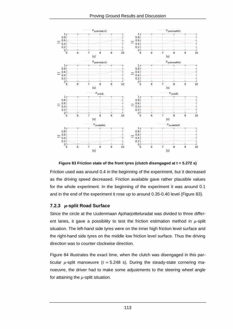
Proving Ground Results and Discussion
113
Figure 83 Friction state of the front tyres (clutch disengaged at t = 5.272 s)
Friction used was around 0.4 in the beginning of the experiment, but it decreased
as the driving speed decreased. Friction available gave rather plausible values
for the whole experiment. In the beginning of the experiment it was around 0.1
and in the end of the experiment it rose up to around 0.35-0.40 level (Figure 83).
7.2.3 -split Road Surface
Since the circle at the Uudenmaan Ajoharjoitteluradat was divided to three differ-
ent lanes, it gave a possibility to test the friction estimation method in -split
situation. The left-hand side tyres were on the inner high friction level surface and
the right-hand side tyres on the middle low friction level surface. Thus the driving
direction was to counter clockwise direction.
Figure 84 illustrates the exact time, when the clutch was disengaged in this par-
ticular -split manoeuvre ( 5.248 s). During the steady-state cornering ma-
noeuvre, the driver had to make some adjustments to the steering wheel angle
for attaining the -split situation.
5 6 7 8 9 100
0.20.4
0.60.8
1
[-]
[s]
potentialL01
5 6 7 8 9 100
0.20.4
0.60.8
1
[-]
[s]
potentialR01
5 6 7 8 9 100
0.20.40.60.8
1
[-]
[s]
potentialL02
5 6 7 8 9 100
0.20.40.60.8
1
[-]
[s]
potentialR02
5 6 7 8 9 100
0.20.40.60.8
1
[-]
[s]
usedL
5 6 7 8 9 100
0.20.40.60.8
1
[-]
[s]
usedR
5 6 7 8 9 100
0.20.40.60.8
1
[-]
[s]
availableL
5 6 7 8 9 100
0.20.40.60.8
1
[-]
[s]
availableR
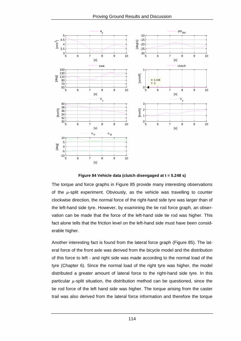
Proving Ground Results and Discussion
114
Figure 84 Vehicle data (clutch disengaged at t = 5.248 s)
The torque and force graphs in Figure 85 provide many interesting observations
of the -split experiment. Obviously, as the vehicle was travelling to counter
clockwise direction, the normal force of the right-hand side tyre was larger than of
the left-hand side tyre. However, by examining the tie rod force graph, an obser-
vation can be made that the force of the left-hand side tie rod was higher. This
fact alone tells that the friction level on the left-hand side must have been consid-
erable higher.
Another interesting fact is found from the lateral force graph (Figure 85). The lat-
eral force of the front axle was derived from the bicycle model and the distribution
of this force to left - and right side was made according to the normal load of the
tyre (Chapter 6). Since the normal load of the right tyre was higher, the model
distributed a greater amount of lateral force to the right-hand side tyre. In this
particular -split situation, the distribution method can be questioned, since the
tie rod force of the left hand side was higher. The torque arising from the caster
trail was also derived from the lateral force information and therefore the torque
5 6 7 8 9 103
3.5
4
4.5
5
[m/s
2]
[s]
ay
5 6 7 8 9 10-30
-25
-20
-15
-10
[deg/s
]
[s]
psidot
5 6 7 8 9 10507090
110130150
[deg]
[s]
swa
5 6 7 8 9 100
1
X: 5.248
Y: 0[on/o
ff]
[s]
clutch
5 6 7 8 9 10303234363840
[km
/h]
[s]
Vx
5 6 7 8 9 100
1
2
3
[km
/h]
[s]
Vy
5 6 7 8 9 10-10
-5
0
5
10
[deg]
[s]
F
R
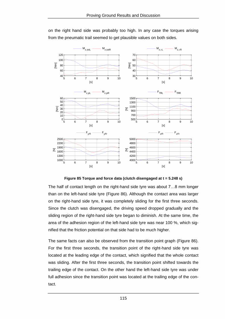
Proving Ground Results and Discussion
115
on the right hand side was probably too high. In any case the torques arising
from the pneumatic trail seemed to get plausible values on both sides.
Figure 85 Torque and force data (clutch disengaged at t = 5.248 s)
The half of contact length on the right-hand side tyre was about 7…8 mm longer
than on the left-hand side tyre (Figure 86). Although the contact area was larger
on the right-hand side tyre, it was completely sliding for the first three seconds.
Since the clutch was disengaged, the driving speed dropped gradually and the
sliding region of the right-hand side tyre began to diminish. At the same time, the
area of the adhesion region of the left-hand side tyre was near 100 %, which sig-
nified that the friction potential on that side had to be much higher.
The same facts can also be observed from the transition point graph (Figure 86).
For the first three seconds, the transition point of the right-hand side tyre was
located at the leading edge of the contact, which signified that the whole contact
was sliding. After the first three seconds, the transition point shifted towards the
trailing edge of the contact. On the other hand the left-hand side tyre was under
full adhesion since the transition point was located at the trailing edge of the con-
tact.
5 6 7 8 9 1040
60
80
100
120[N
m]
[s]
Mz,totL
Mz,totR
5 6 7 8 9 1030
40
50
60
70
[Nm
]
[s]
Mz,L
Mz,R
5 6 7 8 9 100
10
20
30
40
50
60
[Nm
]
[s]
Mz,pL
Mz,pR
5 6 7 8 9 10500
700
900
1100
1300
1500
[N]
[s]
FTRL
FTRR
5 6 7 8 9 101000
1300
1600
1900
2200
2500
[N]
[s]
FyFl
FyFr
5 6 7 8 9 104000
4200
4400
4600
4800
5000
[N]
[s]
FzFl
FzFr
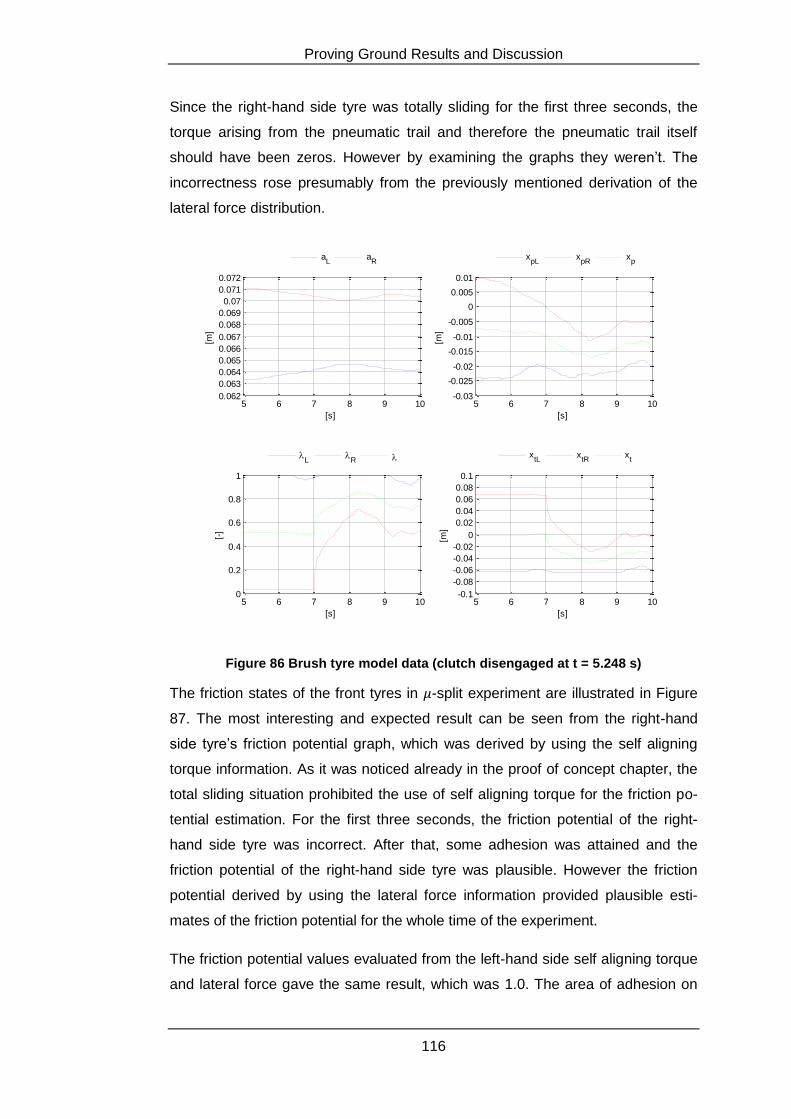
Proving Ground Results and Discussion
116
Since the right-hand side tyre was totally sliding for the first three seconds, the
torque arising from the pneumatic trail and therefore the pneumatic trail itself
should have been zeros. However by examining the graphs they weren’t. The
incorrectness rose presumably from the previously mentioned derivation of the
lateral force distribution.
Figure 86 Brush tyre model data (clutch disengaged at t = 5.248 s)
The friction states of the front tyres in -split experiment are illustrated in Figure
87. The most interesting and expected result can be seen from the right-hand
side tyre’s friction potential graph, which was derived by using the self aligning
torque information. As it was noticed already in the proof of concept chapter, the
total sliding situation prohibited the use of self aligning torque for the friction po-
tential estimation. For the first three seconds, the friction potential of the right-
hand side tyre was incorrect. After that, some adhesion was attained and the
friction potential of the right-hand side tyre was plausible. However the friction
potential derived by using the lateral force information provided plausible esti-
mates of the friction potential for the whole time of the experiment.
The friction potential values evaluated from the left-hand side self aligning torque
and lateral force gave the same result, which was 1.0. The area of adhesion on
5 6 7 8 9 100.062
0.063
0.064
0.065
0.066
0.067
0.068
0.069
0.07
0.071
0.072
[m]
[s]
aL
aR
5 6 7 8 9 10-0.03
-0.025
-0.02
-0.015
-0.01
-0.005
0
0.005
0.01
[m]
[s]
xpL
xpR
xp
5 6 7 8 9 100
0.2
0.4
0.6
0.8
1
[-]
[s]
L
R
5 6 7 8 9 10-0.1
-0.08
-0.06
-0.04
-0.02
0
0.02
0.04
0.06
0.08
0.1
[m]
[s]
xtL
xtR
xt
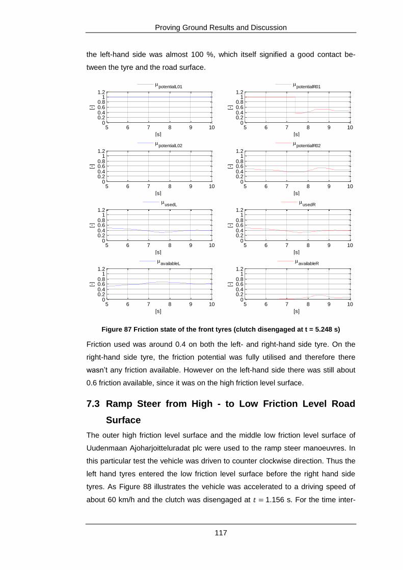
Proving Ground Results and Discussion
117
the left-hand side was almost 100 %, which itself signified a good contact be-
tween the tyre and the road surface.
Figure 87 Friction state of the front tyres (clutch disengaged at t = 5.248 s)
Friction used was around 0.4 on both the left- and right-hand side tyre. On the
right-hand side tyre, the friction potential was fully utilised and therefore there
wasn’t any friction available. However on the left-hand side there was still about
0.6 friction available, since it was on the high friction level surface.
7.3 Ramp Steer from High - to Low Friction Level Road
Surface
The outer high friction level surface and the middle low friction level surface of
Uudenmaan Ajoharjoitteluradat plc were used to the ramp steer manoeuvres. In
this particular test the vehicle was driven to counter clockwise direction. Thus the
left hand tyres entered the low friction level surface before the right hand side
tyres. As Figure 88 illustrates the vehicle was accelerated to a driving speed of
about 60 km/h and the clutch was disengaged at 1.156 s. For the time inter-
5 6 7 8 9 100
0.20.40.60.8
11.2
[-]
[s]
potentialL01
5 6 7 8 9 100
0.20.40.60.8
11.2
[-]
[s]
potentialR01
5 6 7 8 9 100
0.20.40.60.8
11.2
[-]
[s]
potentialL02
5 6 7 8 9 100
0.20.40.60.8
11.2
[-]
[s]
potentialR02
5 6 7 8 9 100
0.20.40.60.8
11.2
[-]
[s]
usedL
5 6 7 8 9 100
0.20.40.60.8
11.2
[-]
[s]
usedR
5 6 7 8 9 100
0.20.40.60.8
11.2
[-]
[s]
availableL
5 6 7 8 9 100
0.20.40.60.8
11.2
[-]
[s]
availableR
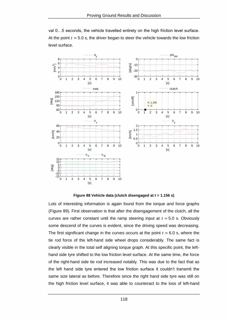
Proving Ground Results and Discussion
118
val 0…5 seconds, the vehicle travelled entirely on the high friction level surface.
At the point 5.0 s, the driver began to steer the vehicle towards the low friction
level surface.
Figure 88 Vehicle data (clutch disengaged at t = 1.156 s)
Lots of interesting information is again found from the torque and force graphs
(Figure 89). First observation is that after the disengagement of the clutch, all the
curves are rather constant until the ramp steering input at 5.0 s. Obviously
some descend of the curves is evident, since the driving speed was decreasing.
The first significant change in the curves occurs at the point 6.0 s, where the
tie rod force of the left-hand side wheel drops considerably. The same fact is
clearly visible in the total self aligning torque graph. At this specific point, the left-
hand side tyre shifted to the low friction level surface. At the same time, the force
of the right-hand side tie rod increased notably. This was due to the fact that as
the left hand side tyre entered the low friction surface it couldn’t transmit the
same size lateral as before. Therefore since the right hand side tyre was still on
the high friction level surface, it was able to counteract to the loss of left-hand
0 1 2 3 4 5 6 7 8 9 100
2
4
6
8
[m/s
2]
[s]
ay
0 1 2 3 4 5 6 7 8 9 10-30
-20
-10
0
[deg/s
]
[s]
psidot
0 1 2 3 4 5 6 7 8 9 1060
90
120
150
180
[deg]
[s]
swa
0 1 2 3 4 5 6 7 8 9 100
1
X: 1.156
Y: 0[on/o
ff]
[s]
clutch
0 1 2 3 4 5 6 7 8 9 100
20
40
60
[km
/h]
[s]
Vx
0 1 2 3 4 5 6 7 8 9 100
0.5
1
1.5
2
[km
/h]
[s]
Vy
0 1 2 3 4 5 6 7 8 9 10-15-10-505
1015
[deg]
[s]
F
R
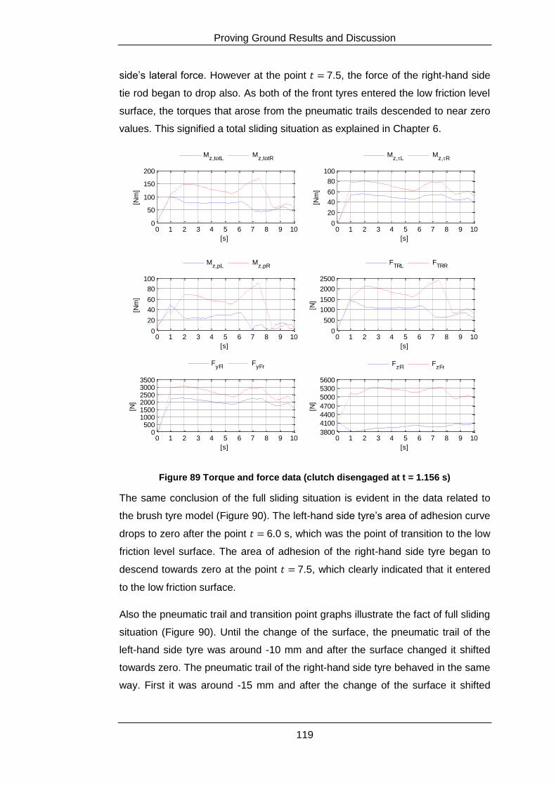
Proving Ground Results and Discussion
119
side’s lateral force. However at the point 7.5, the force of the right-hand side
tie rod began to drop also. As both of the front tyres entered the low friction level
surface, the torques that arose from the pneumatic trails descended to near zero
values. This signified a total sliding situation as explained in Chapter 6.
Figure 89 Torque and force data (clutch disengaged at t = 1.156 s)
The same conclusion of the full sliding situation is evident in the data related to
the brush tyre model (Figure 90). The left-hand side tyre’s area of adhesion curve
drops to zero after the point 6.0 s, which was the point of transition to the low
friction level surface. The area of adhesion of the right-hand side tyre began to
descend towards zero at the point 7.5, which clearly indicated that it entered
to the low friction surface.
Also the pneumatic trail and transition point graphs illustrate the fact of full sliding
situation (Figure 90). Until the change of the surface, the pneumatic trail of the
left-hand side tyre was around -10 mm and after the surface changed it shifted
towards zero. The pneumatic trail of the right-hand side tyre behaved in the same
way. First it was around -15 mm and after the change of the surface it shifted
0 1 2 3 4 5 6 7 8 9 100
50
100
150
200
[Nm
]
[s]
Mz,totL
Mz,totR
0 1 2 3 4 5 6 7 8 9 100
20
40
60
80
100
[Nm
]
[s]
Mz,L
Mz,R
0 1 2 3 4 5 6 7 8 9 100
20
40
60
80
100
[Nm
]
[s]
Mz,pL
Mz,pR
0 1 2 3 4 5 6 7 8 9 100
500
1000
1500
2000
2500
[N]
[s]
FTRL
FTRR
0 1 2 3 4 5 6 7 8 9 100
500100015002000250030003500
[N]
[s]
FyFl
FyFr
0 1 2 3 4 5 6 7 8 9 103800
4100
4400
4700
5000
5300
5600
[N]
[s]
FzFl
FzFr
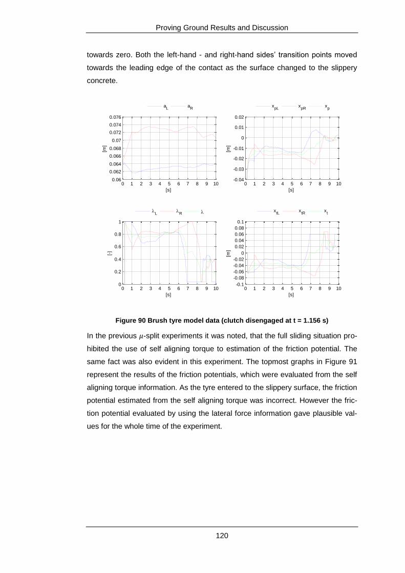
Proving Ground Results and Discussion
120
towards zero. Both the left-hand - and right-hand sides’ transition points moved
towards the leading edge of the contact as the surface changed to the slippery
concrete.
Figure 90 Brush tyre model data (clutch disengaged at t = 1.156 s)
In the previous -split experiments it was noted, that the full sliding situation pro-
hibited the use of self aligning torque to estimation of the friction potential. The
same fact was also evident in this experiment. The topmost graphs in Figure 91
represent the results of the friction potentials, which were evaluated from the self
aligning torque information. As the tyre entered to the slippery surface, the friction
potential estimated from the self aligning torque was incorrect. However the fric-
tion potential evaluated by using the lateral force information gave plausible val-
ues for the whole time of the experiment.
0 1 2 3 4 5 6 7 8 9 100.06
0.062
0.064
0.066
0.068
0.07
0.072
0.074
0.076
[m]
[s]
aL
aR
0 1 2 3 4 5 6 7 8 9 10-0.04
-0.03
-0.02
-0.01
0
0.01
0.02
[m]
[s]
xpL
xpR
xp
0 1 2 3 4 5 6 7 8 9 100
0.2
0.4
0.6
0.8
1
[-]
[s]
L
R
0 1 2 3 4 5 6 7 8 9 10-0.1
-0.08
-0.06
-0.04
-0.02
0
0.02
0.04
0.06
0.08
0.1[m
]
[s]
xtL
xtR
xt
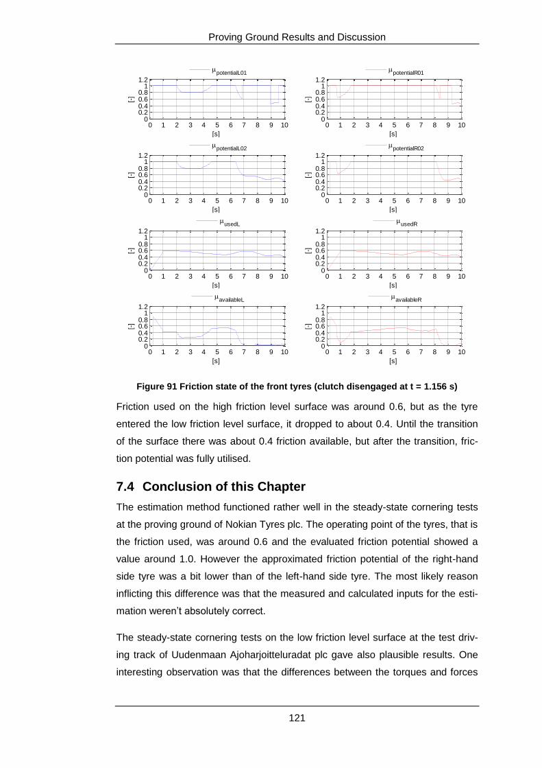
Proving Ground Results and Discussion
121
Figure 91 Friction state of the front tyres (clutch disengaged at t = 1.156 s)
Friction used on the high friction level surface was around 0.6, but as the tyre
entered the low friction level surface, it dropped to about 0.4. Until the transition
of the surface there was about 0.4 friction available, but after the transition, fric-
tion potential was fully utilised.
7.4 Conclusion of this Chapter
The estimation method functioned rather well in the steady-state cornering tests
at the proving ground of Nokian Tyres plc. The operating point of the tyres, that is
the friction used, was around 0.6 and the evaluated friction potential showed a
value around 1.0. However the approximated friction potential of the right-hand
side tyre was a bit lower than of the left-hand side tyre. The most likely reason
inflicting this difference was that the measured and calculated inputs for the esti-
mation weren’t absolutely correct.
The steady-state cornering tests on the low friction level surface at the test driv-
ing track of Uudenmaan Ajoharjoitteluradat plc gave also plausible results. One
interesting observation was that the differences between the torques and forces
0 1 2 3 4 5 6 7 8 9 100
0.20.40.60.8
11.2
[-]
[s]
potentialL01
0 1 2 3 4 5 6 7 8 9 100
0.20.40.60.8
11.2
[-]
[s]
potentialR01
0 1 2 3 4 5 6 7 8 9 100
0.20.40.60.8
11.2
[-]
[s]
potentialL02
0 1 2 3 4 5 6 7 8 9 100
0.20.40.60.8
11.2
[-]
[s]
potentialR02
0 1 2 3 4 5 6 7 8 9 100
0.20.40.60.8
11.2
[-]
[s]
usedL
0 1 2 3 4 5 6 7 8 9 100
0.20.40.60.8
11.2
[-]
[s]
usedR
0 1 2 3 4 5 6 7 8 9 100
0.20.40.60.8
11.2
[-]
[s]
availableL
0 1 2 3 4 5 6 7 8 9 100
0.20.40.60.8
11.2
[-]
[s]
availableR
Proving Ground Results and Discussion
122
of left and right side were considerably smaller than on the high friction level sur-
face. The friction potential of both tyres showed a value around 0.4, which
seemed plausible for that surface and that set of tyres.
A clear distinction between the left- and right-hand side friction potential esti-
mates was observed in the -split experimental tests. The left-hand side tyre was
on the high friction level surface and the estimated friction potential was around
1.0, which was plausible in those conditions. The right-hand side tyre was on the
low friction level surface and the estimated friction potential was around 0.4,
which was also plausible. However the derivation and distribution method of the
lateral tyre forces were questioned in this particular case.
In the experimental tests, where the vehicle was travelling from the high friction
level surface to the low friction level surface, the estimated friction potential
changed according to the road surface. However the same fact was observed as
in the -split tests, that the total sliding situation of the tyre prohibited the use of
self aligning torque information to the friction estimation. Still the lateral tyre force
information could be exploited to the estimation of friction potential in this situa-
tion.
Conclusions and Recommendations
123
8 Conclusions and Recommendations
The objective of this master’s thesis was to study the feasibility of using the front
tyres lateral force and aligning torque information to friction potential estimation.
Since the estimation method exploited the actual forces and torques that were
generated in the tyre-road interface, it classifies to the direct friction estimation
method category. The direct estimation methods need a certain amount of excita-
tion before the obtained friction potential can be considered eligible. Suitable ex-
citation method for this study was the steady-state cornering manoeuvre.
Mathematical models of the vehicle and the tyre were required for this particular
estimation method. The planar behaviour of the vehicle was modelled with the
bicycle model, which provided the axle specific lateral forces. The lateral force of
the front axle was differentiated between left- and right side in accordance with
the normal load distribution of the front tyres. The normal load of the front tyres
were attained from the angle sensors, which were installed to the transverse con-
trol arms. The same angle sensors were exploited for deriving the caster - and
kingpin inclination angles of the steering axes. The caster angle produces an
additional torque around the steering axis, which had to be subtracted from the
total aligning torque. Hence the torque that arose from the tyre itself was distin-
guished. The tie rods of the front wheels were assembled with piezoelectric force
sensors for gaining the total aligning torques around the steering axes.
The force generation of the tyre-road interface was modelled with the brush tyre
model. Thus it can be considered as the heart of the estimation method. Often
the brush tyre model is used for attaining the lateral force and the aligning torque
information as outputs, but in this master’s thesis they were given as inputs to it.
Therefore the brush tyre model could be exploited for evaluating the friction po-
tential of the tyre-road interface.
There were several assumptions concerning the brush tyre model, which most
likely introduced inaccuracy to the estimation. Especially the assumption of stiff
carcass and symmetric parabolic normal load distribution were substantial gen-
eralizations compared to reality. Both of these have an effect to the estimation,
but in what way and how significant they are requires further investigations. One
method for modelling the carcass flexibility can be found from [36]. Examination
of this method is one of the starting points for future studies. Another foundation
Conclusions and Recommendations
124
for future work is to upgrade the brush tyre model to combined slip situation. The
pure lateral slip model works well for rear wheel driven cars, since the longitudi-
nal slip of the front wheels is rather small. However with front wheel driven cars,
the longitudinal slip has a substantial effect to the lateral force and especially to
aligning torque.
The accuracy of the presented friction estimation method was directly depended
of the measured and calculated input variables:
Lateral force
Normal force
Aligning torque
These forces and torques were measured and calculated with various methods,
which undoubtedly produced error to the estimation. Therefore they should have
been validated with reference sensors. Perfect tool for this purpose would have
been the 6-component measuring wheel. For future studies, it’s essential to per-
form the validation of these input variables before conducting the actual proving
ground tests. In addition the estimation method should have been tested with
some simulation software (e.g. IPG: CarMaker) before proceeding to the experi-
mental phase. Attention especially for modelling the front suspension and the
steering system should be paid. The tie rod moves as a function of the steering
angle and the suspension travel, which makes the derivation of the force lever
arm of the aligning torque rather challenging. Thus by modelling the front sus-
pension and the steering system accurately with CarMaker or ADAMS, the force
lever arm can be attained as a function of the steering angle and the suspension
travel.
The experimental tests of the estimation method were divided to two different
proving grounds. The proving ground of Nokian Tyres plc provided the circum-
stances for conducting experimental tests on a typical Finnish road surface. The
second experimental tests were performed at the test driving track of Uuden-
maan Ajoharjoitteluradat plc, which provided extreme slippery conditions. There-
fore the estimation method was tested on both high - and low friction level sur-
faces. In addition, the second proving ground gave an opportunity to try the esti-
mation method in -split conditions and in a situation where the vehicle was trav-
elling from a high friction level surface to a low friction level surface.
Conclusions and Recommendations
125
Steady-state cornering manoeuvres from both proving grounds showed that the
estimation method was able to give plausible values of friction used, - potential
and - available. However some deviation between the friction estimates of inner -
and outer tyre was observed. Measurement - and calculation errors were the
most likely reasons for this deviation. Especially the simplified calculation of the
force lever arm may have caused error to the self aligning torque and thus to the
estimation. The most interesting results were found from the -split - and the sur-
face transition tests. The different road surfaces in the -split situation were dis-
tinguished and both (left - and right side) estimates were in the range of plausi-
ble. Yet it was also discovered that the method for deriving the lateral tyre forces
might not have been adequate in this heterogeneous road surface situation.
Therefore the previously suggested reference sensor system would have been
essential for validating that the input signals are realistic even in these kinds of
road conditions. The results from the surface transition tests illustrated also
clearly the points where the front wheels shifted from one surface to another.
The results gathered from the proving ground tests showed that this particular
friction estimation method has potential. However lots of work and further studies
have to be conducted before this method can assist the modern active safety
systems and the upcoming ADAS systems.

Bibliography
126
Bibliography
1. Milliken, William F. and Milliken, Douglas L. Race Car Vehicle Dynamics.
s.l. : Race Car Vehicle Dynamics, 1994. 1-56091-526-9.
2. Wallman, Carl-Gustaf and Åström, Henrik. Friction measurement methods
and the correlation between road friction and traffic safety. s.l. : Swedish National
Road and Transport Research Institute, 2001. 0347-6049.
3. Statistics Finland. Liitekuvio 1. Tieliikenteessä kuolleet onnettomuustyypin
mukaan, tammi - heinäkuu 2010. Statistics Finland. [Online] 19 8 2010. [Cited: 27
8 2010.] http://www.stat.fi/til/ton/2010/07/ton_2010_07_2010-08-
19_kuv_001_fi.html.
4. Société de Technologie Michelin. The Tyre Grip. 2001.
5. National Cooperative Highway Research Program. Guide for Pavement
Friction. onlinepubs. [Online] 2 2009.
http://onlinepubs.trb.org/onlinepubs/nchrp/nchrp_w108.pdf.
6. Real-time estimation of aquaplaning with an optical tyre sensor. Tuononen,
Ari and Matilainen, Mika. 10, s.l. : Journal of automobile engineering, 2009, Vol.
223. 0954-4070.
7. Tuononen, Ari and Koisaari, Tapio. Ajoneuvojen dynamiikka. Helsinki :
Autoalan Koulutuskeskus, 2010. 978-951-9155-25-8.
8. Chang, Kenneth. The New York Times. Explaining Ice: The Answers Are
Slippery. [Online] 21 2 2006.
http://www.nytimes.com/2006/02/21/science/21ice.html.
9. Brach, Raymond. Adhesion, Hysteresis and the Peak Longitudinal Tire Force.
brachengineering. [Online] 2006.
http://www.brachengineering.com/publications/wheelslipmodel1.pdf.
10. Peussa, Pertti, et al. Final Report of EU-project Fricti@n. vtt. [Online] 3
2009. http://friction.vtt.fi/FRICTION_FinalReport_D13.pdf.
11. Pasterkamp, Willem Remco. The Tyre As Sensor To Estimate Friction.
Delft : Delft Univesity Press, 1997. ISBN 90-407-1538-6.
Bibliography
127
12. Robust Nonlinear Observer To Estimate Road Friction Coefficient and Tire
Slip Angle. Changsun, Ahn, Huei, Peng and Tseng, Eric. Loughborough, UK :
10th International Symposium on Advanced Vehicle Control, 2010.
13. An Estimation Method of the Maximum Tire-road Friction Coefficient Using an
Electric Power Assist Steering. Takagi, Fumiaki, et al. Loughborough, UK : 10th
International Symposium on Advanced Vehicle Control, 2010.
14. A feel for the Road: A Method to Estimate Tire Parameters Using Steering
Torque. Hsu, Judy Yung-Hsiang and Gerdes, Christian. Taipei, Taiwan : 8th
International Symposium on Advanced Vehicle Control, 2006.
15. The Predictive Nature of Pneumatic Trail: Tire Slip Angle and Peak Force
Estimation using Steering Torque. Hsu, Judy Yung-Hsiang and Gerdes,
Cristian. Kobe, Japan : 9th International Symposium on Advanced Vehicle
Control, 2008.
16. Andersson, M., et al. Road Friction Estimation. IVSS. [Online] 6 2007.
http://www.ivss.se/upload/IVSS_2004-17750_final_report_070608.pdf.
17. VOLKSWAGEN AG. Self-study programme 321: The Golf 2004 Running
gear. Wolfsburg : s.n., 2003.
18. Reimpel, Jorsen and Stoll, Helmut. The Automotive Chassis: Engineering
Principles. Warrendale : Society of Automotive Engineers, 1996. ISBN 1-56091-
736-9.
19. VOLKSWAGEN AG. Self-study programme 317 The electro-mechanical
power steering with dual pinion. Wolfsburg : s.n., 2003.
20. Kistler Group. Measuring Systems for Vehicle Development: Measuring
Wheels and Hubs, Crash Barriers, Force Sensors. 2007.
21. Luhtamäki, Tommi, et al. Volkswagen Golfin sähkömekaanisen
ohjaustehostimen mallinnus. s.l. : Teknillinen Korkeakoulu,
Konerakennustekniikan laitos, Auto- ja työkonetekniikan laboratorio, 2009.
22. Kistler Group. Instruction Manual: Quartz Load Washers Types
9101A...9107A. Winterthur : s.n., 2009.
Bibliography
128
23. Kistler Group. Load washer, 0 ... 50 kN: Type 9102A. Kistler. [Online]
http://www.kistler.com/fi_fi-fi/13_Productfinder/App.9102A.5/Load-washer-0-...-
50-kN.html.
24. Kistler Instrumente AG. Instruction Manual: ICAM - Industrial Charge
AMplifier for Manufacturing Applications Type 5073A... Winterthur : s.n., 2006.
25. Kistler Group. Process Instrumentation and Automation: Measuring Sytems
for Process Monitoring and Quality Assurance in Manufacturing , Assembly and
Test Stands. 2009.
26. Kistler Group. Set of preloading elements for load washers: Type 9021A.
Kistler. [Online] 2010. http://www.kistler.com/fi_fi-
fi/13_Productfinder/App.9420A21.5/Set-of-preloading-elements-for-load-washers-
Type-9021A.html.
27. Beckhoff. BK5150, BK5151 | CANopen “Compact” Bus Couplers. Beckhoff.
[Online] 2010.
http://download.beckhoff.com/download/Document/Catalog/Main_Catalog/english
/separate-pages/Bus_Terminal/BK5150_BK5151.pdf.
28. Beckhoff. KL3132/62/72/82 | 2-channel analog input terminals. Beckhoff.
[Online] 2010.
http://download.beckhoff.com/download/Document/Catalog/Main_Catalog/english
/separate-pages/Bus_Terminal/KL3132_KL3162_KL3172_KL3182.pdf.
29. Beckhoff. KL91xx, KL92xx | Bus function terminals. Beckhoff. [Online]
http://download.beckhoff.com/download/Document/Catalog/Main_Catalog/english
/separate-pages/Bus_Terminal/KL91xx_KL92xx.pdf.
30. Bosch Rexroth Corporation. Angle of Rotation Sensor WS1. Bosch Rexroth
Corporation. [Online] 2010.
http://www.boschrexroth.com/country_units/america/united_states/en/products/br
m/products_catalogs/electronics/a_downloads/ra95140_02-04234664.pdf.
31. Corrsys Datron. CORREVIT® S-350 Aqua: Non-Contact Optical Sensor for
slip-free measurement of longitudinal and transversal dynamics. CORRSYS-
DATRON. [Online] 2008. http://www.corrsys-
datron.com/Support/Data_Sheets/Datasheets-Sensors/cds-d_S-350_e.pdf.
Bibliography
129
32. CORRSYS-DATRON. S-350 with Gyro Integration. CORRSYS-DATRON.
[Online] 2006. [Cited: ] http://www.corrsys-datron.com/Support/Applications/EW-
B-07-0107-1%20S-350%20with%20Gyro%20correction1.pdf.
33. Nokian Tyres plc. Nokian Tyres tests its products in extreme conditions.
[Brochure] 2010.
34. Nokian Tyres plc. Nokian WR G2. Nokian Tyres plc. [Online] 2010.
http://www.nokiantyres.com/tyre?id=10360796&group=1.01.02&name=Nokian+
WR+G2.
35. Uudenmaan Ajoharjoitteluradat Oy. Korkealuokkaiset Ajoharjoitteluradat.
[Brochure] 2010.
36. Pacejka, Hans Bastiaan. Tire and Vehicle Dynamics, 2nd edition. Oxford :
Elsevier Ltd, 2006. ISBN 978-0-7506-6918-4 .
37. Svendenius, Jacob. Tire modeling and Friction Estimation. Lund : Lund
University, 2007. ISSN 0280–5316.
38. Fujifilm. Prescale: Features. Fujifilm: Prescale. [Online] 2010.
http://www.fujifilm.com/products/prescale/prescalefilm/features/.
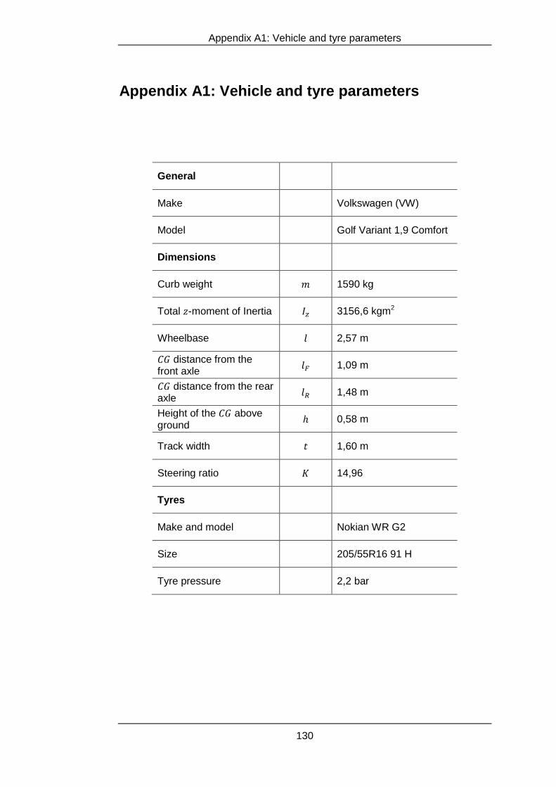
Appendix A1: Vehicle and tyre parameters
130
Appendix A1: Vehicle and tyre parameters
General
Make Volkswagen (VW)
Model Golf Variant 1,9 Comfort
Dimensions
Curb weight 1590 kg
Total -moment of Inertia 3156,6 kgm2
Wheelbase 2,57 m
distance from the front axle
1,09 m
distance from the rear axle
1,48 m
Height of the above ground
0,58 m
Track width 1,60 m
Steering ratio 14,96
Tyres
Make and model Nokian WR G2
Size 205/55R16 91 H
Tyre pressure 2,2 bar
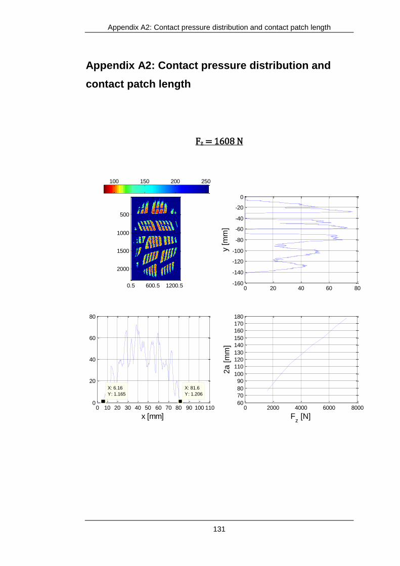
Appendix A2: Contact pressure distribution and contact patch length
131
Appendix A2: Contact pressure distribution and
contact patch length
Fz = 1608 N
0.5 600.5 1200.5
500
1000
1500
2000
0 10 20 30 40 50 60 70 80 90 100 1100
20
40
60
80
X: 81.6
Y: 1.206
x [mm]
X: 6.16
Y: 1.165
0 20 40 60 80-160
-140
-120
-100
-80
-60
-40
-20
0
y [
mm
]
0 2000 4000 6000 800060
70
80
90
100
110
120
130
140
150
160
170
180
Fz [N]
2a
[m
m]
100 150 200 250

Appendix A2: Contact pressure distribution and contact patch length
132
Fz = 2413 N
500 1 000 1 500
500
1000
1500
2000
0 10 20 30 40 50 60 70 80 90 100 1100
20
40
60
80
100
X: 6.032
Y: 1.208
x[mm]
X: 102
Y: 1.424
0 20 40 60 80-160
-140
-120
-100
-80
-60
-40
-20
0
y[m
m]
0 2000 4000 6000 800060
70
80
90
100
110
120
130
140
150
160
170
180
Fz [N]
2a [m
m]
100 150 200 250
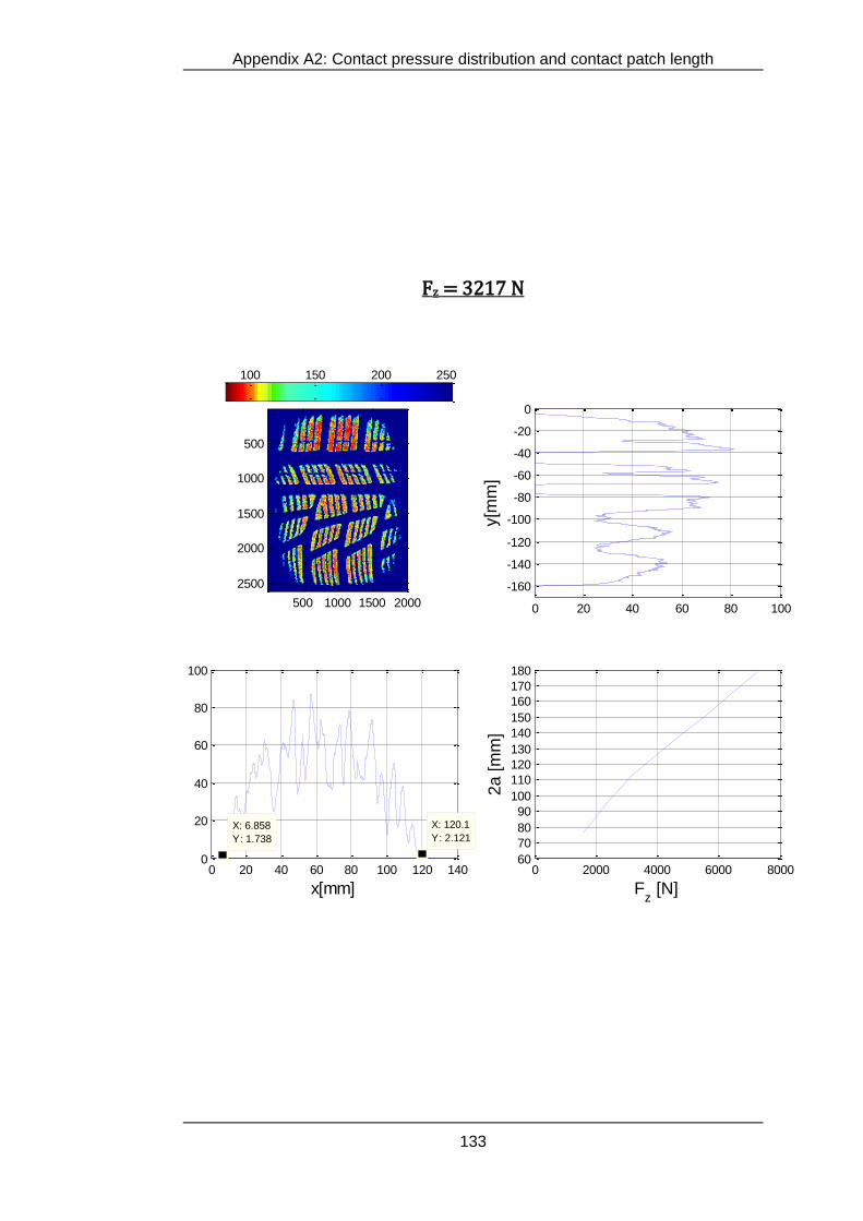
Appendix A2: Contact pressure distribution and contact patch length
133
Fz = 3217 N
500 1000 1500 2000
500
1000
1500
2000
2500
0 20 40 60 80 100 120 1400
20
40
60
80
100
X: 120.1
Y: 2.121
x[mm]
X: 6.858
Y: 1.738
0 20 40 60 80 100
-160
-140
-120
-100
-80
-60
-40
-20
0
y[m
m]
0 2000 4000 6000 800060
70
80
90
100
110
120
130
140
150
160
170
180
Fz [N]
2a
[m
m]
100 150 200 250

Appendix A2: Contact pressure distribution and contact patch length
134
Fz = 4021 N
500 1000 1500 2000
500
1000
1500
2000
2500
0 20 40 60 80 100 120 1400
20
40
60
80
100
X: 8.7
Y: 1.471
x[mm]
X: 135.3
Y: 1.763
0 20 40 60 80 100-170
-150
-130
-110
-90
-70
-50
-30
-10
y[m
m]
0 2000 4000 6000 800060
70
80
90
100
110
120
130
140
150
160
170
180
Fz [N]
2a
[m
m]
100 150 200 250
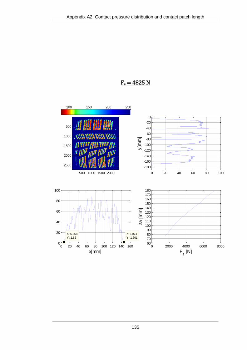
Appendix A2: Contact pressure distribution and contact patch length
135
Fz = 4825 N
500 1000 1500 2000
500
1000
1500
2000
2500
0 20 40 60 80 100 120 140 1600
20
40
60
80
100
X: 6.858
Y: 1.62
x[mm]
X: 146.1
Y: 1.601
0 20 40 60 80 100
-180
-160
-140
-120
-100
-80
-60
-40
-20
0
y[m
m]
0 2000 4000 6000 800060
70
80
90
100
110
120
130
140
150
160
170
180
Fz [N]
2a
[m
m]
100 150 200 250
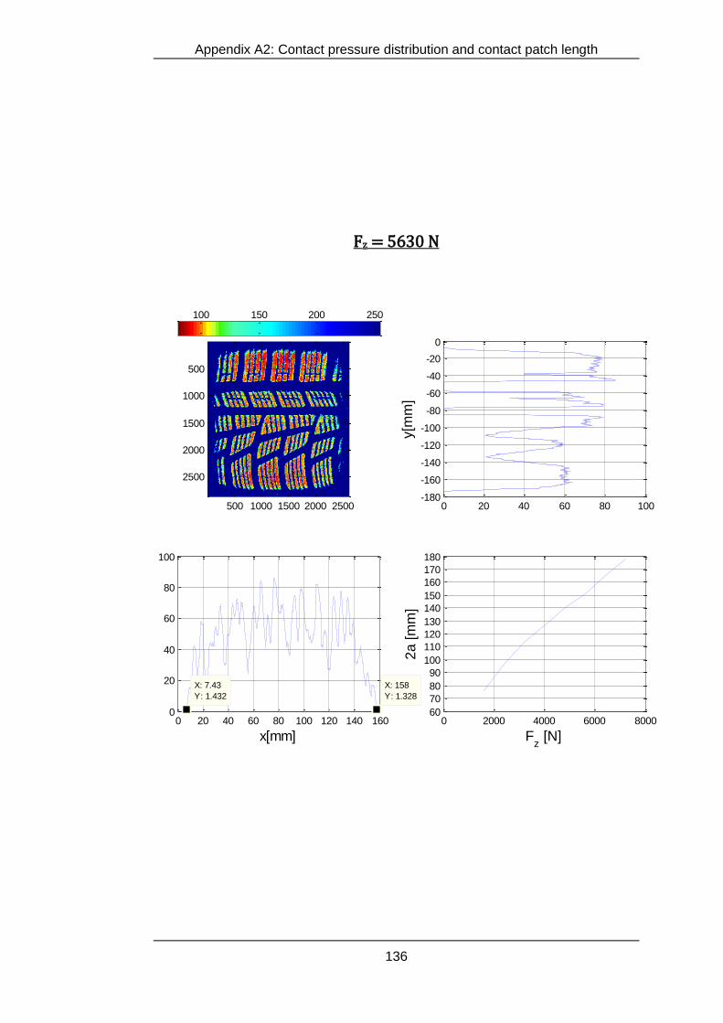
Appendix A2: Contact pressure distribution and contact patch length
136
Fz = 5630 N
500 1000 1500 2000 2500
500
1000
1500
2000
2500
0 20 40 60 80 100 120 140 1600
20
40
60
80
100
X: 7.43
Y: 1.432
x[mm]
X: 158
Y: 1.328
0 20 40 60 80 100-180
-160
-140
-120
-100
-80
-60
-40
-20
0
y[m
m]
0 2000 4000 6000 800060
70
80
90
100
110
120
130
140
150
160
170
180
Fz [N]
2a
[m
m]
100 150 200 250
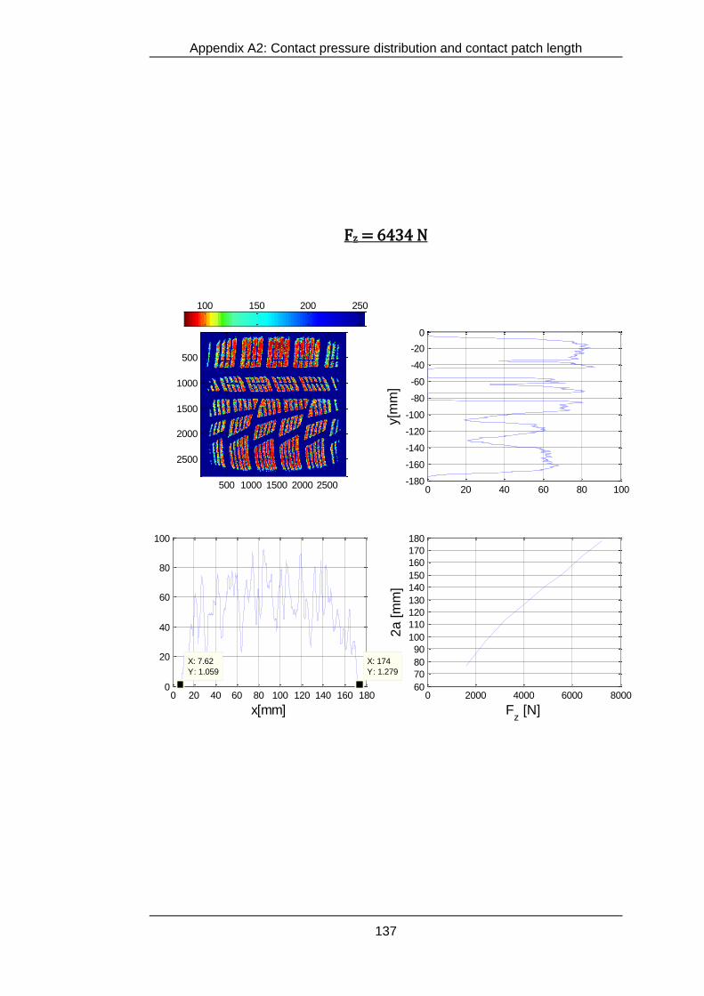
Appendix A2: Contact pressure distribution and contact patch length
137
Fz = 6434 N
500 1000 1500 2000 2500
500
1000
1500
2000
2500
0 20 40 60 80 100 120 140 160 1800
20
40
60
80
100
X: 174
Y: 1.279
x[mm]
X: 7.62
Y: 1.059
0 20 40 60 80 100-180
-160
-140
-120
-100
-80
-60
-40
-20
0
y[m
m]
0 2000 4000 6000 800060
70
80
90
100
110
120
130
140
150
160
170
180
Fz [N]
2a [m
m]
100 150 200 250