TWO YEARS

L INTROLXJCTION

OF ACTS PROPAGATION STUDIES IN ALASKA

Charles E. Mayer and Bradley E. JaegerElectrical Engineering Department

lJniversity of Al&$ka FairtnmksP.O. Box 755900

Fairbanks, AK 99775-5900

The Alaska ACTS Propagation Terminal (APT) is located on lop of the engineeringbuilding on the University of Alaska Fairbanks campus. The latitude and longitude of the site are64° 51‘ 28” N and 147°48’59” W. The geometrical elevation angle to ACTS is 7.97°. Includinga nom]aJ atmospheric ref’ractivit y, the elevation angle increases to 8.10°. “rhc azimuth angle toACTS is 129.36°. The terminal is located at 580 feet above mean sea level. The site is located inITU-R rain zone C and Cram global model zone B 1. ACTS transmits vertical @ariz,ationbeacons at 27.505 and 20.185 GHz.. At the APT the polarization tilt ang,lc is 19.4° rotated CCWwith respect to vertical when looking toward the satellite. The beacons are t ransmitted in aCONUS pattern. The ACTS beacon footprint at tk Alaska ~ site is 9 dB down from thetransmission pattern peak at 27.505 GHz and 11 dB down from the pattern peak at 20.185 GHz.We will henceforth refer to the beacon frequencies as 27.5 (or 27) and 20,2 (or 20) GHz for thesake of brevity.

11. FAIRBANKS WEATHERAn undcrs(anding of the weather in Fairbanks is pmtinent to understanding the displayed

results. Fairbanlw has very cold and very dry winters. The months November through March canbe considered winter, where the only form of precipitation is snow, usually very dry. Thetransition months of September, October, and April can experience rain, wet snow, or possibl ysome dry snow. Snow dots not greatly attenuate microwave signals. Rain is normally experiencedMay through September. The armuaJ average precipitation in Fairbanks is 11.0 inches, as shownin Table 1 below.

Table L Annual Weather Statistics in }’airbanks by Month-— .—Month Precipitation No. of Days Mean Minimum Mean Maximum

(Inches) with 20.1 in. Temperature, ‘C Temperature, “CPrecipitation—-—— — . — ——. . . ..—

January 0.69 2.1 -28.9 -18.9——— — — . _— - ..-.February 0.58 1.9 -26.1 -12.7-— —.. —- ——— ..—March 0.41 1.1 -20.6 -50-——. —- - - -April -n —0.25 , 0 . 6_e- .—4.9May 0.71 2.0 2 . 2 14,8——— —- . ..—June 1.42 3 . 2 7 . 7 - _ . — - 21.0- — — .-. —July 1.90 4.0 9.3 22..2-— —.. —-—August 2.03 4.2 6 . 6 — ‘- 18.8-— —.. .. —— - -—— ..—September 1.26 2.6 1.1 12.1———. —- —.October

.-—0.73 1.9 - 7 . 8 1.1——- ..—

November 0.48 - ,. 1.6 _ _ -11.1-20.6 ._ ..—.December 0.55 1.8 -27.8 -18.9-— —.. —- . ..—Yearly ToIaJ 11.00 27.0 -9.4 2.2— —. ——- — .

41

III. MON’1’H1.Y AND YEARLY ATTENUATION ANI) RAIN RATE CDFSThe major experimental results of the measurement campaign arc the total attenuation and

rain rate, The cumulative distribution function (CDF), which is also called an empiricaldistribution function (EDF), is the primary method of displaying the experiment results. Theabscissa on the attenuation CDF plot is total attenuation in dB ranging from -S to 30 dB, and theordinate is percentage time the attenuation is greater than the abscissa ranging from 0.001 to100%. The abscissa on the rain rate CDF plot is rain rate in mm/hr, and the ordinate is percentagetime the rain rate is greater than the abscissa. The attenuation and rain rate CDFS are presentedfor each month and also on a yearly basis. These CDFS are presented time sequentially in theappendix of this document. The attenuation CDFS include both beacon and radiometerdistributions for both 20.2 and 27.5 GHz. The monthly attenuation CDFS display results thatparallel the discussion of Fairbanks weather above. The CDFS for the cold, dry winters exhibitvery low attenuation. The CDFS for the wanner summers exhibit larger percentages of attenuat ionat a few dB (1 -4 dB). This attenuation is due to gaseous absorption. At a low elevation angle,the Fairbanks-ACTS link propagates through about 8 airmawes of atmosphere, where one airmassis the amount of atmosphere intcgrat ed to zenith, The summer CDF’S also extibit largerattenuation at tic lower percentages. This attenuation is due to hydrometers, mostly rain. Thernonthl y rain rale CDFS clear] y correspond to the attcnuatio] I meamred during that month. Thelarge variability yin these CDFS from month 10 month, the sinlilarit y of each month from year toyear, and the predictable trends from the above Fairbanks weather discussion indicate theimportance of viewing attenuation statistics on a monthl y basis. First wc will discuss some overallfeatures of these CDFS.

A. Total Attenuation CDFSSeveral features must be explained to help interpret the results displayed in these

attcnua(ion CDFS. Duc to the extra pattern footprint loss in Alaska and the limited dynamic rangeof the AFT, the total attenuation with respect to free space can be accuratel y measured to a totalattenuation lCVC1 of approximately 18 dB with a sufficiently high signal-to-noise ratio, so that theattenuation value given is accurate. Values of attenuation gi eater than this threshold are given thevalue of 35 dB by the preprocessing program and displayed as 30 dB on the CDFS. Thus anattenuation value of 24 dB would be displayed as 30 dB, as would an attenuation value of 40 dB.This method of binning values was chosen so that the total time of attenuation greater than themcasurcmcnt threshold would be properly accounted for, This tends to flatten out the tails ofattenuation CDFS. This is not the shape that the CIIFS would show were the measurementdynamic range larger. Values on the CDFS greater than 151020 dB therefore do not accuratelyrepresent measured data and should not be taken as valid measurements.

Figure 1 shows the yearly attenuation CDFS for year 1 and year 2. Both the 20 and 27GH7. beacons are displayed. The attenuation displayed is tic total altenuaiion, including gaseousabsorption, rain attenuation, snow attenuation, scintillation, antenna wetting, and any otherhydrometeor-caused attenuation. The 20.2 GHz beacon experiences more gaseous attenuation andhence has larger attenuation at the lower attenuation levels. The 27.5 GHz beacon experiencesmore hydrometer attenuation and hence has larger attenuation at the higher attenuation levels.The crossover point of the two frequency attenuation curves is clearly at the 4 dB and 2% point,The 20.2 GHz beacon is reasonably close to the atmospheric water vapor absorption line at 22.2GH7,. ‘Ihe 27.5 GHz beacon, although higher in frequency, is farther from this absorption line andexperiences lCSS specific attenuation due to water vapor. By including year 1 and year 2 togetherin Figure 1, a measure of the variability between these two years can be readily seen, A word of

4 2

caution must be given when interpreting these CDlk. ll~e average of these two years cannot betaken as the “average” year in Fairbanks. Many more years would need tcj bc included to give anaccurate assessment of the average year. Thus although these curves show points and narrowlines, it is not accurate to use these curves as an average attenuation.

Often a communications system must be designed to meet worst month statistics. Figure 2shows the worst month envelope of attenuation. This curve was created comparing equi-attcnuation values and selecting the highest percentage time at each of those levels. It should benoted that the 3 summer months of June, July and August were the only month that contributed tothis worst month CDF.

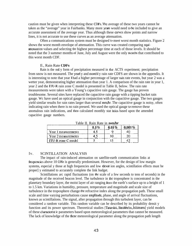
Il., Rain Rate CDFSRain is the onl y form of precipitation measured in tl E ACTS experiment; precipitation

from snow is not measured. The yearl y and monthl y rain rate CDFS are shown in the appendix. Itis interesting to note that year 1 had a higher percentage of larger min rate events, but year 2 was awetter year, demonstrating higher attenuation than year 1. A comparison of the rain rate in year 1,year 2 and the ITU-R rain zone C model is presented in Table II, below. The rain ratemeasurements were taken with a Young’s capacitive rain gauge. The gauge has proventroublesome. Several sites have replaced the capacitive rain gauge with a tipping bucket raingauge. Wc have used an optical gauge in conjunction with the capacitive gauge. The two gaugesyield similar results for rain rates larger than several mm/hr. The capacitive gauge is noisy, oftenindicating rain when there is no rain presenl. We used the optical gauge to remove theseanomalous rain indications, and then calculated monthly stat istics based upon the amendedcapacitive gauge numbers.

Table II. Rain Rate in mrnhr

:::iEd33:r 33

Iv. SCINTILLATION ANALYSISThe impact of rain-induced attenuation on satellite-earth communication links at

frcqucncics above 10 GHz is generally predominant. However, for the design of low marginsystems, especial y those at high frequencies and low elevat ion angles, scintillation effects must beproper] y estimated to accurately complete the link budget.

Scintillations arc rapid fluctuations (on the scale of a few seconds to tens of seconds) in themagnitude of the received beacon level. The turbulence in tile troposphere is concentrated in theplanetary boundary layer, the moist layer of air ranging froln the earth’s surface up to a height of 1to 1.5 km. Variations in humidity, pressure, temperature and magnitude and scale size ofturbulence in the troposphere change the refractive index along the propagation path. These smallscale and time varying perturbations cause amplihlde, phase, and angle of arrival fluctuations,known as scintillations. The signal, after propagation through this turbulent layer, can beconsidered a random variable. This random variable can be described by its probability densit yfunction and its power spectrum. Theoretical studies [Tatarskii, Strohbehl, lshimaru] yield modelsof these charactenst ic parameters based upon meteorological parameters that cannot be measured.The lack of knowledge of the these meteorological parameter along the propagation path length

43

has lcd to the dcvclopmcnt of semi-cmpincal models representing tic magnitude and characteristicsof’ scintillations.

The intensi( y of the scintillations must be accurately portrayed by a measurement unit.The scintillation process is assumed to be a zero-mean process with fluctuations about that mean,The fluctuations can be represented in terms of their root mcarr square, or nns. Since the mean ofthe process is zero, the mus can be represented by the standard deviation of the process.

The measure of the intensit y of scintillation used will be the standard deviation of the logamplitude of the received signal, that is, the standard deviation of the received signal in decibels.The time duration of the standard deviation calculation will bc one minute.

A. ‘1’ime Series AnalysisFigure 3 shows the received 27.5 GHz beacon level over a period of 10 minutes on August

16, 1994. Large variations of the received beacon level are apparent from this figure. The timebehavior of scintillations is demonstrated on this summer day of large scintillations. The day washumid and warm, with a light wind and fill sky cover. An expanded view of this period is shownin Figure 4, which covers 1 minute of time on this day. Note that the 20.2 and 27.5 GH7. beaconsarc both displayed, and are closely correlated over most of the time. There is about a 2 dBdiffcrcncc for several seconds. Also of note is the mpid rise of received beacon level in seconds 20through 25. Both frequencies experience a 5 d13 rise in 6 seconds. ‘The mean level of these signalsis about -13 dB (the scale is a relative scale), so that the signal enhancement is only about 3 dBabove the nominal level. Signal attenuation is thought of m the major impairment tocomrnunicat ions ystems. However, signal enhancements caI I also cause problems, especially inmulti-carrier transponder operation, where the input power nmst remain below the nonlinearthreshold. If too much input power is supplied, the tramfxmder becomes more nonlinear,producing intermodulation (IM) distortion, which can greatly reduce the overall C/N. Figure 5 isincluded to present another time series view of scintillation in a representative minute; this exampleis minute 38 in the hour. Again the behavior of both beacons is highly correlated, with onlyintervals of several seconds where they differed by several dB. Also note the rapid decrease of 3 to4 dB during the 3 seconds near the end of the minute. During this hour on August 16, 1994 thebeacons experienced large scintillations, as in most of the da y. The distribution of scintillationswill be studied using PDFs (probability density functions) of one minute standard deviation inseveral time durations.

IL PDFsThe APT samples each beacon (and each radiometer) once a second. Scintillations were

studiccl by calculating the siandard deviation in orm minute I)eriods of receivecl beacon data (60samples at each frequency). The standard deviations, measured in cIB, were binned in 0.05 dBwidth bins. The number of calculated standard deviations (i e., the number of seconds) in each binwere tabulated, forming a histogram distribution of the number of seconds of scintillation standarddeviation at each bin dB value. These histogram distributiol~ were produced over a 1 hour timeperiod, over a 1 day time peliod, and over a 1 month time period. The nesting hour, day, andmonth were 18-19 GMT, 16th, and August 1994. The number of minutes at each standarddeviation vah.rc bin were plotted in PDFs, or probability density functions. Figure 6 shows thePDF for one hour of standard deviation values. The time period is 18-19 GMT on August 16,1994. The abscissa of the plot is onc minute standard devialiom in dB. Ihc ordinate is theprobability of occurrence, displayed on a logarithmic axis. For example, there was a 10%probability of the standard deviation being 0.75 dB for the 20.2 GHz beacon and about an 8%probability y of the standard deviation being 0.75 dB for the ?7.5 GHz beacon. It is clear that thescintillations were large during the hour, as the standard deviation was lCSS than 0.5 dB for only a

4 4

few percent of the time for the 20.2 GHz beacon and less than 0.7 dB for a small percentage oftime for the 27.5 GH7 beacon. The standard deviations for the entire day c)f August 16, 1994 areshown in Figure 7. It is clear that there were many times of lower magnitude standard deviationsover the whole day as compared to the one hour displayed in Figure 6. Also of note is that therewere larger standard deviation values for a small percentage of the time. Finally, the PDF of thestandard deviations for the entire month of August 1994 is presented in Figure 8. Again thedistribution tends to move toward lower values of standard deviations.

C. Scintillation Standard Deviationincreasingly, models for attenuation due to scintillation, gases, and clouds are becoming

important for low margin satellite applications Total fade distributions have applications indetermining link margins and in determining service quality [Salonen, Matsudo]. Models for thefading due to scintilla ion incorporate the smridard deviation of sigmd amplitude (a,) in t wo ways.First, the formulation of the long tcnn cumulative distribution (CDF) of scintillation log amplitude(~ in dB) is undertaken by assuming two distributions. If a conditional distribution of x given G,and a distribution for O, arc given, the CDF of log amplitude can be found by integrating over theproducl of these two distributions [Allnutt]. Second, the models for fading due to scintillationincorporate a prediction of the mean standard deviation of signal amplitude breed on the local wetrefractivity. The authom present Ihe first year of the standard deviation of signal amplitude. Theyfound that for the firsl year of observation the standard deviation of’ signal amplitude was boundedby both the CCIR model and the Karasawa model. They present a typical probability densityfunclion for the standard deviation of signal amplitude and measured prediction equations for themean standard deviation of signal amplitude from wet refractivity for the first year.

D. Two Standarcl Probability Density Functions of Standard DeviationTwo models are generally accepted for the standard deviation of signal amplitude, the

Karasawa gamma distribution and the Moulsley-Vilar lognormal distribution. These modelsdescribe the standard deviation of attenuation with rain and gas attenuation effects removed, Theequation used to perform this oj)eration [Crane] is as follows:

CT. .&u(AFs)Giii(Ami, (1)

where var(AFS) is the variance in the free space attenuation, or total attenuation, and var(ARD) isthe variance in the radiometer attenuation channel, which accounts for the rain and gaseousattenuation. The Karasawa gamma distribution [Allnutt] describes the distribution of signalstandard deviation using parameters ~ and ~ that could be related to measurements:

(2)

The mean of the signal standard deviation is equal tom and the variance of the signal standard

deviation isa ~ . TM distribution is used to form the CDF of scintillation fading in both the*

CCIR model and the Karasawa model. Moulsley and Vilar obtained cumulative distributions forsignal fading by using a lognormal probability density function for the standard deviation of signalfading [Moulsley]:

45

(3)

where

m = ln(o ~) = avg(ln(o ~ )) and 66 = var(ln(o ~ )).

In Fairbanks the authors have obtained measured distributions of signal standarddeviation. Statistical K-S tests of these distributions against gamma and lognormal distributionswill be presented later in the Proceedings of the IEEE. Typical distributions for each beaconfrequency arc shown in Figures 9 and 10.

E. Prediction of Average Signal Standard Deviation from Wet RefractivityThere am two accepted models for predicting an average signal standard deviation, the

CCIR model and tic Karasawa model, Each model makes a prediction of the signal standarddeviation from the average wet refractivity and then scales to frequency, elevation angle, andaperture size. Figures 11 and 12 show the annual variation in average hourl y standard deviation atFairbanks. The data for the first year are below both the CCIR model and the Karasawa modelpredictions.

Using station parameters from Haystack, Massachusetts, the CCIR model scales tofrequency, elevation angle, and aperture size as follows:

co ,,f o f + o g(x)0 ——

pre ‘“”sin@)l”2

3730. H. esN =

“ e’ (273 + t)2

p 1]5854. 10 20-(;;;:r) “

(4)

c~ = ( )(273 + t)s ‘–

where

~pre is the predicted monthl y average standard devialioxl of signal amplitude (dB)L is the effective turbulent path length (m)h is the turbulence height (m)e is the elevation angleD.fl is the effective antenna diameter(m)D is the antenna diameter (m)k is the wave number (m-l)~ is the antenna cffeciencyr. is the effective earth radius=8.5. 10G (m)NW,et is the wet refractivity (N units)es is the monthly average saturated water vapour pressure (rob)t is the monthl y average surface temperature (“C).

The Karasawa model is very similar, scaling from its station parameters at Yamaguchi,Japan, to other frequencies, elevation angles, and aperlure sizes. The main theoreticaldifference between the two models is the scaling with frequency, f7”2 versus ~“45.Karasawa made the argument that Yamaguchi frequencies fell in between the diffractionregion and the geometrical optical region. The diffraction region was assumed to be underthe Tatarskii model, f7’]2, and the geometrical opticalYokoi model, ~. The Karasawa model is as follows:

Iegion was assumed to be under the

with

“,=[-=%$W”5”rW.)

‘D- = G(7.6)3730. H . es

N =‘“ ( 2 7 3 + t)2

[ “)‘ s = 6“11 ‘X p (:::7:)

( )

DoR= O.75 —

2

( )G(R)= 1.0–1.4. -~

Jzzfor OS #Z <0.5

where

4 7

is the predicted rnonthl y average standard cleviation of signal amplitude (dB)is the unscaled predicted monthl y average standard deviation of signal amplitude (dB)is the wet refractivity (N units)is the frequency scaling, f is the frequency (GHz)is the elevation angle scaling, 6 is the elevation angleis the antenna diameter scaling, D, is the antenna diameter (m)is the monthly average relative humidity (%)is the monthl y average saturated water vapour pressure (rob)is the monthl y average surface temperature (°C)is the anlema aperture averaging fiictoris the effective radius of circular aperture (m)is the effective turbulent path length (m)is the turbulence height (2000 m)is the effective earth radius=8.5. 106 (m).

In Fairbanks the relationship bet we-en average hourly standard deviat ion and wetrcfractivit y, in the first year, was as given in Figure 13 and} ‘igure 14. Additional data will beanaly~cd before deciding if these relationships are statistical y different from the models.

The frequency scaling exponent for the first year was nearly equal to the Karasawa model.The ratio of standard deviations, 1.14, was calculated from an average ratio of standard deviations.The arguments in the average came from interpolating equal percentage points on cumulativedistribution functions. Solving the CCIR scaling relation for a:

ln(%:%)-’2ln[’:$/)-;l’’[*))Q = —.—-——.. ——.—. —..

[)f(6)

11) -–f,

Substituting 1.14 for the ratio of standard deviation gives a=:O.44.Figure 15 and Figure 16 show the month to month variability in standard deviations. The

months of January and Augvst are nominally the months with the smallest and largestscintillation All other months typically fit between these bounds. Figure 17 shows the one yearCDFS of standard deviation and associated power law fits.

v . CONCLUSIONSThe Fairbanks AK APT site is the only APT site with a low elevation angle, ‘Ilh feature

allows measurements to be made on a long propagation path length through the atmosphere.Propagation phenomena that are strongly elevation angle dependent include. gaseous absorption andscintillations. The AK APT clearly experiences large amounts of gaseous absorption during thehumid summer months, as seen in the total attenuation CDFS. Scintillations have been analyzedand presented in PDFs of their st andard deviation. For the lI~onth of August 1994, one minutestandard deviations were greater than 1.5 dB for 0.02$% of the month at 20.2 GHz and for 0.03%of the month for 27.5 GHz. It should be noted that the beacon peak-to-peak variation issignificant y larger than the standard deviation. For example, the 10 minute time series of beacondata shown in Figure 3 has a standard deviation of 0.88 dB, whereas the peak-to-peak variationsarc on the order of 5.0 dll. “rwo models of signal standard deviation (CCIR and Karasawa), which

48

quantifies the magnitude of scintillations, were compared to the measured data, with the measuredvalues being significantly less than both models.

RIWERENCES

Allnutl, J. E., Y. Karasawa, and M. Yamada, “A New Prediction Method for TroposphericScintillation on Eallh-Space Paths,” IEEE Transactions on Antennas and Propagation,pp. 1608-1614, November 1988.

Crane, R. K., E-mail Communication.

Ishimaru, A., Wave Propagation and Scattering in Random Media. New York: Academic Press,1978.

Matsudo, T. and Y. Karasawa, “Characteristics and Prediction methods for the Occurrence Rateof SES in Available Time Affected by Tropospheric Scintillation,” Electronics andCommunications in Japan, pp. 843-851, IIccembcl 1990.

Moulsley, T. J., and E. Vilar, “Experimental and Theoretical Statistics of Microwave AmplitudeScintillations on Satellite Down-links,” l&;EE Transactions on Antennas andPropagatiorz, pp. 1099-1106, November 1982.

Saloncn, E. T., J. K, Tervonen, and W. J. Vogel, “Scintillation Effects on Total Fade Distributionsfor Earth-Satellite Links,” IEEE Transactions on Antennas and Propagation, pp. 23-27,January 1996.

Strohbchn, J. W., “Line-of-Sight Wave Propagation ThrouSh the Turbulent Atmosphere,” IEEEProceedings, vol. 56, no. 8, pp. 1301-1318, August 1968.

Tatarskii, V. 1., Wave f’ropagation in a Turbulent Medium (translated by R. A. Silverman). NewYork: McGraw-Hill, 1961.

4 9

—

Fig. 1. AK Yearly Beacon Attenuation (second) EDF

~- ‘--–--———. .—

+ 20GHz Be%onTYear 1 +- 20GHz Beacon, Year 2--k- 27GHz Beacon. Year 1 +- 27GHz Beacon, Year 2

100

10

1

0.1

0.01

0.001-5 0 5 10 15 20 25 30

Attenuation dB

5 0

Fig. 2. 2 Year Envelope of Worst Monthly Attenuation (second) EDF

+- 20GHz Beacon --.&- 27GHz Beacon- — — — — . — — ——. .-100

10

1

0.1

0.01

0.001-5 0 5 10 15 20 25 30

Attenuation dB

51

IQ

Ri

,@IL

.s!3=

00:01:81

0s60:81

00:60:81

OC:80:81

00:80:81

OC:LO:81

00:10:81

0S90:81

00:9081

OC&O:81

00: S0:81

OC:ti081

OO:bO:81

0C:CO:8

00:CO:8

0S70:8

00:208

OC:1O:81

00:10:81

0C:OO:81

00:00:81

-cgm

?2

r

%,

.2.

- - WZ081

0t7:ZO:81

+ 8s20:81 ~

- 9S:20:81 Fo

- t7&:ZO:81 ~

- ZC:ZO:81 :- - 0GZ081 $

-8 2:20:81 ~

i9320:81 ~

]--02:20:81-81:20:81

- -91:2081- *1:Z081

- - Z1:ZO:81

-01:2081-80:20:81

-90:2081

- t70:ZO:81

-20:20:81

—--t-----t------t-- ——i——’+———+———~ 00:20:81

—

2’c1mb’a

I

2c1mlow

t

—

.—

—–-t——+————t—— t- —t--- 1

00:6s81

8S:8G81

9$8G81

ts8G81

ZS:8G81

OS:8E81

W:8G81

8t7:8fY81

W:8G81

i3t:8c:81

ot7:8c:81

8C:8G81 ~

9C:8C:81 ~o

ti&xW81 ~

3C:8G:81 :

o&:8c:81 ~

87:88:81 ~

92:8S81 ~

W8G81 +=

ZZ:8C:81 (!s

02:8s81

81:8C:81

91:8&81

t71:8c:81

71:8s81

01:8E81

80:8C81

903S8)

tio:8c:81

20:8s:81

00:8s:81

Fig.

6. O

ne M

inut

e S

tand

ard

Dev

iatio

n P

DF

18-1

9H G

MT

8/1

6/94

100

II

II

,I

I,

I!

1\

,I

\(

,1

II

1

0.00

1I

II

I,

1

00.

51

1.5

22.

53

One

Min

ute

Sta

ndar

d D

evia

tion

(dB

)

Fig.

7. O

ne M

inut

e S

tand

ard

Dev

iatio

n P

DF

8/1

6/94

100

t,

1I

tI

II

o0.

51

1.5

22.

53

One

Min

ute

Sta

ndar

d D

evia

tion

(dB

)

Fig.

8. O

ne M

inut

e S

tand

ard

Dev

iatio

n P

DF

Aug

ust 1

994

100

tI

11

t, I

II

1,

J

00.

51

1.5

22.

53

One

Min

ute

Sta

ndar

d D

evia

tion

(dB

)

o

CQo

z“

I& o InN

o m o

(y.) aammooo

58

o

gw

CD

i

0

co

0

Fig.

11.

Ann

ual V

aria

tion

in H

ourl

y S

tand

ard

Dev

iatio

n

0.80

0

0.70

0

Q,@

g

n m

n“,

””.

0.40

0

0.30

0

0.20

0

0.10

0

0.00

0

Fair

bank

s; 6

4.86

° N

, 147

.82°

WD

ec 1

993-

Nov

199

4f:

20.

185

GH

z0:

7.92

°D

a: 1

.22

m,+

A -“-

---

.’.A

..’

●

.WA

’ ●,*---

‘**

.-

.*

\.

. ‘“o-

/\

‘.. .

/\

’.

\

h.

●

~.

If\

‘.\

‘.

‘“

’’”

/’

A’

,.”

/

-.-

--

--

-A

--

--

---k

”-.

./

/

H*’

“---s

~/

--

-o

-

-- *

--

CC

IR M

od

el

-4

-K

aras

awa

Mod

el

~ M

ean

hour

ly s

igm

a

Dec

Jan

Feb

Mar

Apr

May

Jun

Jut

Aug

Sep

Ott

Nov

0,80

0

0.70

0

0.100

Fig.

12.

Ann

ual V

aria

tion

in H

ourl

y S

tand

ard

Dev

iatio

n

Fair

bank

s; 6

4.86

° N

, 147

.82°

WD

ec 1

993-

Nov

199

4●

A. .

. -..

*f:

27.

505

GH

z● , ,

●

0*

0:7.

92°

*.

A* ●

Da:

1.2

2 m

.P

- -~

‘“

., .

0.

/Y

‘.

./

\ ‘,

. . ●

P’

\ ‘,

.\*

. . ./1

\k \

‘.A*

/f

\ ‘.

0.000 D

ecJa

nFe

bM

arA

prM

ayJu

nJu

lA

ugS

epO

ttN

ov

--*--

CC

! F?

Mod

e!

– 9-

Kar

asaw

a s

igm

a

~ M

ean

hour

ly s

igm

a

.

0.5

0.45 0.

4

0.35 0.

3

0,25 0.2

Fair

bank

s; 6

4.86

° N

, 147

.82°

WD

ec 1

993-

Nov

199

4f:

20.

185

GH

z0:

7.92

°D

a: t

.22

nl

0.10

1020

3040

5060

Nw

et (N

uni

ts)

0CD

0

0

63

Fig.

15.

One

Min

ute

Sta

ndar

d D

evia

tion

Per

cent

age

of T

ime

Func

tions

0.01

0.00

10

, . ●Fa

irba

nks;

64.

86°

N, 1

47.8

2° W

t , ,f:

20.

185

GH

z. , *

0:7.

92°

8 .D

a: 1

.22

m, , * \ . , * , Q * * . \ . , . , , * , 1 \ * 9 ● b , * , . ● * .

--

..

●. \

\.

●

, .\

--h

\\

---%

I

,!

,,

,,

0.5

11.

52

2.5

33.

5

—Ju

l 19

94

--

- A

ug

1994

----

- ”J

an 1

994

4

One

Min

ute

Sta

ndar

d D

evla

tlon

(dB

)

1 :

1.

--l F.

i r- “—”

Wd

// /

8 01-

—0 s.

0

.

In0

0

—

●L

l~i19I : i

c1

T-

C5

d-

Lqm

C9

qN

al

IQ

q0

0