two-stage controlled fractional factorial screening for...

1

Two-Stage Controlled Fractional Factorial Screening for Simulation Experiments

Hong Wan Assistant Professor School of Industrial Engineering Purdue University 315 N. Grant Street West Lafayette, IN 47907-2023 [email protected] (765) 494-7523 Fax: (765) 494-1299

Bruce E. Ankenman Associate Professor Department of Industrial Engineering and Management Sciences Northwestern University 2145 Sheridan Rd. Evanston, IL. 60208 [email protected] (847) 491-5674 Fax (847) 491-8005 url: www.iems.northwestern.edu/~bea

JUNE 23, 2006

ABSTRACT

Factor screening with statistical control makes sense in the context of simulation experiments

that have random error, but can be run automatically on a computer and thus can accommodate a

large number of replications. The discrete-event simulations common in the operations research

field are well suited to controlled screening. In this paper two methods of factor screening with

control of Type I error and power are compared. The two screening methods are both robust

with respect to two-factor interactions and non-constant variance. The first method is the

sequential method introduced by Wan, Ankenman, and Nelson (2005a) called CSB-X. The

second method uses a fractional factorial design in combination with a two-stage procedure for

controlling power that has been adapted from Bishop and Dudewicz (1978). The two-stage

controlled fractional factorial (TCFF) method requires less prior information and is more

efficient when the percentage of important factors is 5% or higher.

2

Key Words

Computer experiments, Discrete-event simulation, Design of Experiments, Factor Screening,

Sequential Bifurcation

Bruce E. Ankenman is an Associate Professor in the Department of Industrial Engineering and

Management Sciences at the McCormick School of Engineering at Northwestern University.

His current research interests include response surface methodology, design of experiments,

robust design, experiments involving variance components and dispersion effects, and design for

simulation experiments. He is a past chair of the Quality Statistics and Reliability Section of

INFORMS, is an Associate Editor for Naval Research Logistics and is a Department Editor for

IIE Transactions: Quality and Reliability Engineering. He is a member of ASA and ASQ.

Email: [email protected]

URL: www.iems.northwestern.edu/~bea

Hong Wan is an Assistant Professor in the School of Industrial Engineering at Purdue

University. Her research interests include design and analysis of simulation experiments;

simulation optimization; simulation of manufacturing, healthcare and financial systems; quality

control; and applied statistics. She has taught a variety of courses and is a member of INFORMS

and ASA. Her e-mail and web addresses are [email protected] and

http://web.ics.purdue.edu/hwan/index.htm.

3

Introduction

The term computer experiment is common in the statistical literature (see Santner,

Willliams, and Notz, 2003) and refers to an experiment on a computer simulation of a physical

system such as a material or a process. Typically, computer experiments are thought to be

deterministic (having no random error other than rounding error). This is because many

engineering simulations use finite element or other differential equation-based simulation

methods that have no random component. However, in the operations research community, the

term “simulation” is most commonly used to refer to discrete-event simulations of manufacturing

or service systems (see Banks, Carson, Nelson and Nicol, 2005). These simulations are typically

complex queueing systems that simulate products or customers flowing through a system. The

simulation is driven by random number generators that draw random arrival times for the

products or customers and random service and failure times for the machines or stations. The

input distributions for these random number generators are based on the distributions observed

for each type of machine or station in the system. Typical software packages for this type of

discrete-event simulation include Witness®, Arena®, Simul8®, and Factory Explorer®. Many

other software packages have been developed for more specific scenarios, for example,

MedModel® for healthcare simulation. Although they do have random noise like physical

experiments, discrete-event simulation experiments share some attributes with computer

experiments:

1) In many cases, the whole experiment can be programmed to run automatically.

2) Compared to physical experiments, it is usually cheaper and easier to switch

factor settings in a simulation experiment. Therefore, the design of the

simulation experiment is often sequential, using a design criterion to choose

the next run or to stop the experiment.

4

3) In many cases, replications are not as expensive as they are in physical

experiments. This fact allows for the experiment size to be determined by a

desired precision (or correctness) instead of a preset experimental budget.

In this article, we will compare two approaches for factor screening in the context of

discrete-event simulation experiments. Factor screening refers to an experiment that is designed

to sort a large set of factors into those that have an important effect on the system in question and

those that do not substantially affect the system response (see Dean and Lewis, 2005). Factor

screening is used for many different purposes. It is often used as a first stage of an optimization

or investigation procedure intended to reduce the number of factors that must be included in

more detailed investigation. However, there are many other reasons for performing factor

screening including (1) gaining a better understanding of a system by finding the factors that

affect the output and equally important finding those factors which have a negligible effect on

the output over the range of interest, (2) preparing for future adjustment or control of a system by

finding a set of factors that can affect the output, and (3) simplifying the simulation model by

removing portions of the model that have little effect on the output of interest.

Typically in factor screening, a hierarchical argument is used so factors with important

main effects are first screened out and then additional experiments are done to determine if those

important factors interact with each other or have higher order effects. Since the cost of

replication is so high, the emphasis in factor screening for physical experiments has been to

allow for the estimation of as many main effects as possible in as few runs as possible. This has

lead to approaches such as supersaturated designs (see Lu and Xu, 2004) and group screening

(see Lewis and Dean, 2001). In view of the three characteristics of discrete-event simulation

experiments listed above, the screening methods that we will compare in this article will be

driven not by a specific number of experimental runs, but instead by a desired level of Type I

5

error (the probability of declaring a factor important when it is not) and power (the probability of

correctly declaring a factor important). Due to the statistical control that we impose on this

screening experiment, we will call this controlled screening. Of course, given that the desired

level of statistical control (power and level of Type I error) is achieved, it is desirable to reduce

the number of replications and thereby reduce the total amount of computer time needed for the

screening experiment. Thus, the number of replications needed to achieve the desired level of

control will be the criterion for comparing the two screening methods.

In discrete-event simulations, the responses of interest are often system performance

measures like average cycle time for a product to pass through the system. For complicated

systems, there are often hundreds of factors. For example, there may be many stations or

machines in the manufacturing system and each station or machine may have several factors

associated with it. In many cases, these factors have a known direction of effect on the response.

For example, increasing the speed of a transporter will likely decrease the average cycle time if it

has any effect at all. Using the assumption that the directions of the effects of the factors are

known and the hierarchical assumption that linear effects are a good indicator factor importance,

Wan, Ankenman, and Nelson (2005a) proposed Controlled Sequential Bifurcation (CSB), a

controlled factor screening method for simulation experiments that uses a form of binary search

called sequential bifurcation. Sequential bifurcation was originally proposed for deterministic

screening by Bettonvil and Kleijnen (1997). CSB was extended to provide error control for

screening main effects even in the presence of two-factor interactions and second order effects of

the factors (Wan, Ankenman, and Nelson, 2005b). The new method is called CSB-X. An

interesting finding in Wan, et al. (2005b) is that if interactions are not present, CSB-X is usually

as efficient as CSB in identifying main effects (this depends on the variance structure at different

levels of the factors). When two-factor interactions are present, CSB is unable to correctly

6

control the identification of the main effects due to confounding with the interactions. Thus,

CSB-X is recommended for controlled screening in almost all cases. The primary purpose of

this paper is to compare CSB-X with another method of screening, namely a fractional factorial

design that is used as part of a two-stage method for controlling Type I error and power.

In the next section, we briefly describe the objectives of controlled screening. This

structure was first introduced in Wan, et al. (2005a). Section 3 briefly describes CSB-X and then

introduces a version of fractional factorial screening that controls Type I error and power using a

two-stage sampling procedure similar to the one used in Bishop and Dudewicz (1978) for a two-

way ANOVA layout. Section 4 compares the two methods under a variety of scenarios and

shows the circumstances under which each method is preferred. Conclusions are then drawn.

Objective of the Controlled Screening

The purpose of this paper is to compare the performance of two methods of controlled

screening. In order to compare the methods fairly, some structure on the screening problem is

now established. We begin with the model. Suppose there are K factors and a simulation output

response represented by Y, then we assume the following full second order model:

01 1

K K K

k k km k mk k m k

Y x x xβ β β ε= = =

= + + +∑ ∑∑ , (1)

where xk represents the level of factor k and ε is a normally distributed error term whose

variance is unknown and may depend on the levels of the factors, i.e., ( )2~ Nor(0, )ε σ x , where

( )1 2, , , Kx x x=x … . In this paper, we assume that the factor levels are coded on a scale from -1

to 1. Later, we will focus on Resolution IV, two-level designs which often used in main effects

screening with non-negligible interactions. In these designs, the linear main effects estimators

7

are not confounded by any other terms; however, many of the second order interactions may be

confounded together and the pure quadratic terms will confounded with the estimate of 0β .

Other designs could in principle be adapted to the proposed method, but we leave this for future

research. To ease the discussion, we also assume that larger values of the response, Y, are more

desirable. The case of a “smaller is better” response is easily handled by making the response

negative.

The goal of the controlled screening is to provide an experimental design and analysis

strategy to identify which factors have large linear main effects, the kβ ’s in (1). Two thresholds

are established:

1. 0∆ is the threshold of importance used to establish the level of Type I error.

Specifically, if 0kβ < ∆ , then the probability of declaring factor k important should

be less than α, where α is selected by the experimenter. Typically 0.05α = .

2. 1∆ is the critical threshold used to control the power. Specifically, if 1kβ ≥ ∆ , then

the probability of declaring factor k important should be greater than γ, where γ is

selected by the experimenter Typically 0.80γ ≥ .

The scaling of the factors can be done in any way that the experimenter finds useful;

however, since all factor effects are to be compared to the same thresholds, they should be

comparable in some sense. One method would be to have the response be dollars of profit

produced and thus all costs for changing factor levels would be incorporated into the profit

calculation. Another scaling method, introduced in Wan, et al. (2005a), assures that all the factor

effects are on the same cost scale. For purposes of discussion, we will follow the cost-based

scaling method of Wan, et al. (2005a). The method assumes that the lower the factor setting, the

8

lower the cost. The scaling is such that the cost to change each factor from the level (0) to the

highest cost level (1) is a fixed cost, say c*. Wan, et al. (2005a) shows how the levels of discrete

factors (e.g. the number of machines or number of operators) can be incorporated into this cost-

based scaling system by introducing a weighting for each factor. The benefit of this cost-based

scaling is that each linear effect, kβ , can be compared directly to the thresholds and to the other

linear effects since kβ represents the expected change in the response when spending c* to

change factor k. The two thresholds now also become easily expressed concepts:

• The threshold of importance, 0∆ , is the minimum amount by which the response

must rise in order to justify an expenditure of c* dollars.

• The critical threshold, 1∆ , is an increase in the response that should not be missed if

it can be achieved for an expenditure of c* dollars.

Since the response is to be maximized, then it is natural to assume that increasing the cost of any

factor will either have no effect or increase the response. Thus in Wan, et al (2005a), it is

assumed that the directions of all main effects are known and the levels of the factors are set to

make all the main effects positive, i.e., 0kβ ≥ , 0 k K< ≤ .

Methodology

In this section, we will first review CSB-X, the method proposed in Wan, et al. (2005b)

that provides controlled factor screening in the presence of two-factor interactions. We will then

present a method of controlled screening that uses a two-stage hypothesis testing procedure in a

standard fractional factorial design. The second method will be called TCFF for Two-stage

Controlled Fractional Factorial.

9

CSB-X, Controlled Sequential Bifurcation with Interactions

CSB-X is a controlled version of sequential bifurcation. Sequential bifurcation is a series

of steps, where within each step a group of factors is tested. Within the group, all factors are

completely confounded together (as in group screening, see Lewis and Dean, 2001). Therefore,

it is critical to CSB-X that the direction of all the factor effects be positive (i.e. 0kβ ≥ ,

0 k K< ≤ ) to prevent cancellation of effects. If a group of factors is tested and the group effect

(the sum of all the main effects of the factors in the group) is not found to be significantly greater

than 0∆ (the threshold of importance) then all the factors in the group are declared unimportant

and are dropped from further screening. If the group effect is found to be greater than 0∆ and

there is only one factor in the group, then that factor is declared to be important. If the group

effect is found to be greater than 0∆ and there is more than one factor in the group, the group is

split into two subgroups that are to be tested later. This procedure is followed until all factors are

classified as either important or unimportant.

Kleijnen and Bettonvil (1997) suggest various practical methods for splitting and testing

the groups. Specifically, splitting groups into subgroups whose size is a power of 2 can improve

the efficiency of the procedure. Also, if one selects for testing groups that have large group

effects before groups that have small group effects, the procedure can sequentially reduce the

upper bound on the greatest effect that has not yet been identified. This upper bound is very

useful if the procedure is stopped early. Since we are comparing the statistical control of the

procedures, we plan to complete the screening procedure in all cases and thus the sequential

upper bound is not of interest. Also, we found in empirical testing, that splitting groups into

subgroups whose size is a power of 2 did not always improve efficiency and never led to

increases in efficiency that substantially changed our conclusions. Thus, for better comparison

10

to Wan, et al. (2005b), we will use the procedure that simply splits each important group into two

equally sized subgroups. In the case of an odd group size, the subgroup sizes differ by one. We

will also follow the testing procedure of Wan, et al. (2005b). To define the design points of their

experiment, the design point at level k is defined as

( ) 1, 1, 2,3,0, 1, 2,i

i kx k

i k k K=⎧

= ⎨ = + +⎩ .

Thus, “level k” has all factors with indices greater than k set to 0 on the –1 to 1 scale and all

factors with indices less than or equal to k, set to 1. Similarly, a design point at “level –k” is

defined as

( ) 1, 1, 2,3,0, 1, 2,i

i kx k

i k k K− =⎧

− = ⎨ = + +⎩ .

To test a group of factors, say factors with indices in the set 1 1 2{ 1, 2, , }k k k+ + , four

design points are used, “level 1k ,” “level 1k− ,” “level 2k ,” “level 2k− .” To follow the notation

in Wan, et al. (2005b), let ( )Z k represent the observed simulation output for the th replication

at level k. The procedure ensures that all four design points have the same number of

replications and the test statistic, ( )1 2,D k k , is calculated as

( ) ( ) ( ) ( ) ( )( )1 2 2 2 1 1, / 2D k k Z k Z k Z k Z k⎡ ⎤ ⎡ ⎤= − − − − −⎣ ⎦ ⎣ ⎦ .

They show that given (1), the expected value of ( )1 2,D k k is the sum of the factors’ main effects

from the group 1 1 2{ 1, 2, , }k k k+ + , i.e.,

( )2

1

1 21

,k

kk k

E D k k β= +

⎡ ⎤ =⎣ ⎦ ∑ .

11

The group is declared important if the null hypothesis, 2

1

0 01

:k

kk k

H β= +

≤ ∆∑ , is rejected at

level α. The group is declared unimportant if the null hypothesis is not rejected, provided that

the test used has power γ for the alternative hypothesis, 2

1

11

:k

A kk k

H β= +

≥ ∆∑ . To guarantee this

statistical control, Wan, et al. (2005b) provide a fully sequential test that first takes an initial

number, 0n , of replications at each of the four design points and then adds replications one-at-a-

time (to all four design points) until the group effect can be declared either important or

unimportant. Even under non-constant variance conditions as in (1), CSB-X with the fully

sequential test guarantees that the probability of Type I error is α for each factor individually and

the power is at least γ for each step of the algorithm.

TCFF, Two-stage Controlled Fractional Factorial

The TCFF method begins by selecting a fractional factorial design that is capable of

achieving the desired resolution for the number of factors being screened. Recall that a

resolution III design can estimate all main effects independent of each other, but does confound

main effects with certain two-factor interactions (this is similar to CSB). A resolution IV design

also allows for independent estimation of main effects, and in addition removes any bias due to

two-factor interactions between the factors. In order to match the capabilities of CSB-X, we will

use resolution IV designs for the comparison in this paper.

Many books (e.g. Wu and Hamada, 2000) and software packages provide recommended

fractional factorial designs for various resolutions and various values of K, the number of factors

to be screened. If a recommended design cannot be easily found for a particular value of K, a

resolution IV design can always be easily constructed by taking an orthogonal array large enough

to accommodate K two-level factors and then folding it over according to the procedure

12

described on page 172 of Wu and Hamada (2000). Since the foldover procedure doubles the

number of runs in the orthogonal array, this procedure produces a resolution IV design for K

factors that has at least 2×(K+1) design points. A very extensive list of orthogonal arrays for

different values of K has recently been published by Kuhfield and Tobias (2005).

The method described below for controlling the power does not require any particular

resolution design and in fact can be used with higher resolution designs if one wants to screen for

factors with important two-factor interactions or higher order effects. Of course higher

resolution designs will require more design points and potentially many more observations.

Once the fractional factorial design (with N design points) is selected, the next step is to

control the power and Type I error of the main effect estimates. To accomplish this, we adapt a

two-stage method developed to control power for the two-way ANOVA layout by Bishop and

Dudewicz (1978). The first stage of the method requires an initial number, say 0n , of

replications of the fractional factorial design, i.e., 0n observations at each design point. Since the

fractional factorial is likely to be quite large, we recommend that 0n be relatively small such as 3

or 5. The second stage of the method adds replications to certain rows of the factorial design to

get better estimates of the mean response of those rows for which the responses have high

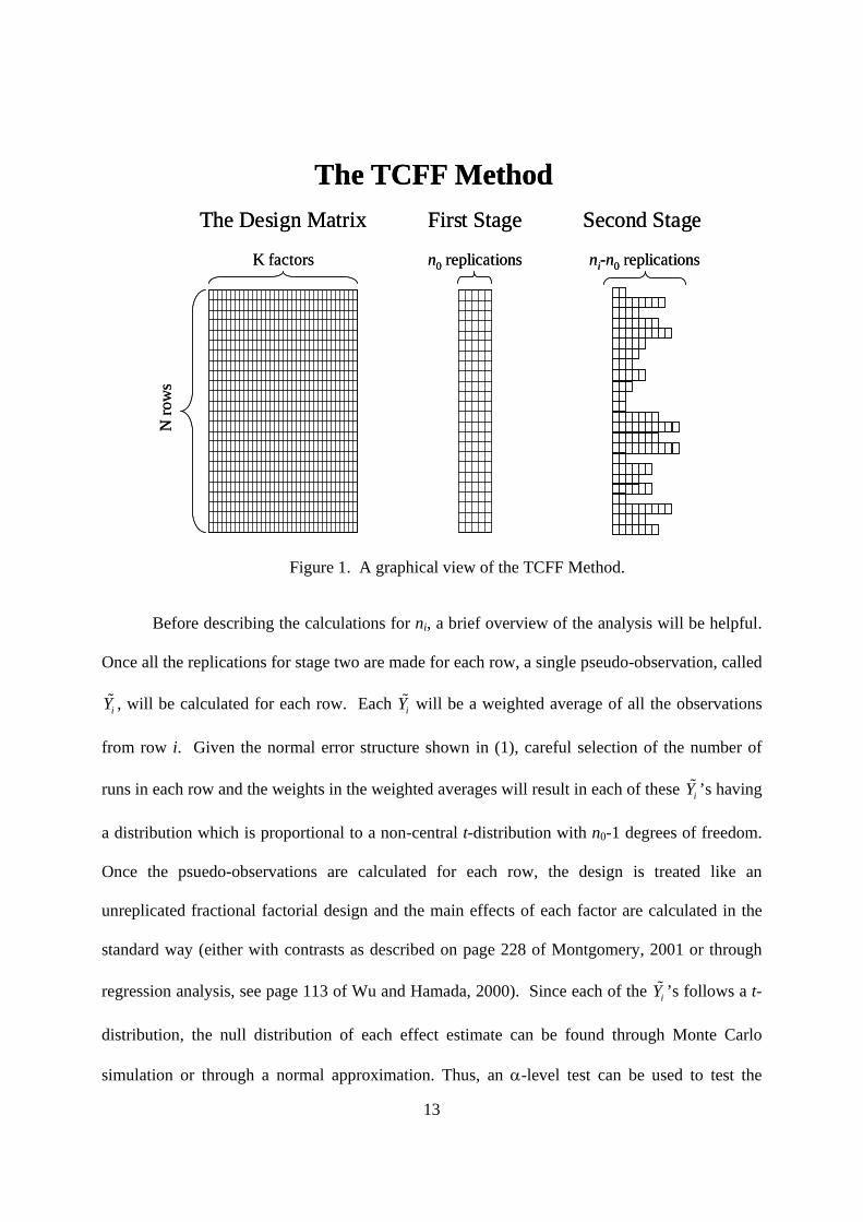
variance. We denote the total number of replications for row i after both stages as in . Thus, the

number of additional replications taken for row i in the second stage is 0in n− . The TCFF

procedure is represented graphically in Figure 1. The keys to the control of Type 1 error and

power for this method are: (1) the calculation for in and (2) careful selection of the estimators

for each factor effect.

13

The TCFF MethodThe Design Matrix First Stage Second Stage

N ro

ws

K factors n0 replications ni-n0 replications

The TCFF MethodThe Design Matrix First Stage Second Stage

N ro

ws

K factors n0 replications ni-n0 replications

Figure 1. A graphical view of the TCFF Method.

Before describing the calculations for ni, a brief overview of the analysis will be helpful.

Once all the replications for stage two are made for each row, a single pseudo-observation, called

iY , will be calculated for each row. Each iY will be a weighted average of all the observations

from row i. Given the normal error structure shown in (1), careful selection of the number of

runs in each row and the weights in the weighted averages will result in each of these iY ’s having

a distribution which is proportional to a non-central t-distribution with n0-1 degrees of freedom.

Once the psuedo-observations are calculated for each row, the design is treated like an

unreplicated fractional factorial design and the main effects of each factor are calculated in the

standard way (either with contrasts as described on page 228 of Montgomery, 2001 or through

regression analysis, see page 113 of Wu and Hamada, 2000). Since each of the iY ’s follows a t-

distribution, the null distribution of each effect estimate can be found through Monte Carlo

simulation or through a normal approximation. Thus, an α-level test can be used to test the

14

hypothesis: 0 0: kH β ≤ ∆ or 1 0: kH β > ∆ . The calculation of the number of replications in the

second stage of the method ensures that if the effect of factor k is greater than 1∆ , the probability

that factor k will be declared important is greater than γ.

The steps for determining ni are now given (The formulas are adapted from Bishop and

Dudewicz, 1978.):

1. Let the cdf of the distribution of the average of N independent standard t-

distributed random variables each with 0 1n − degrees of freedom be called

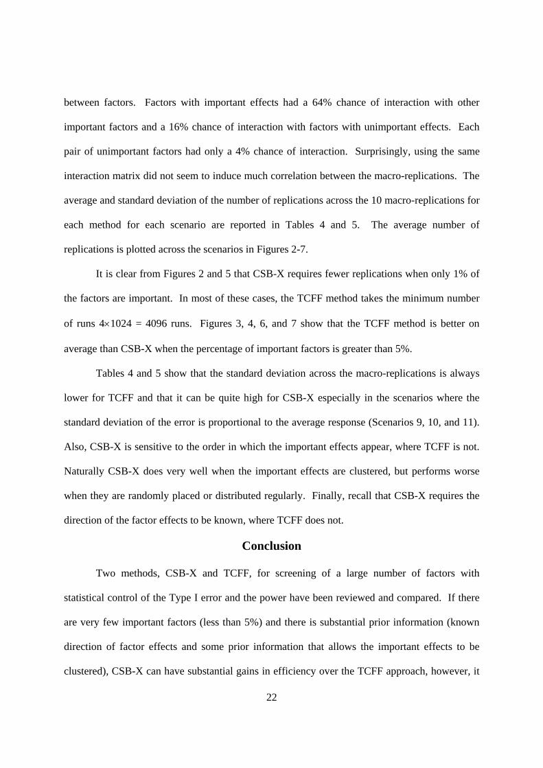
( )0, 1,t N n x− , where x is the argument of the cdf. Let c0 be the 1-α quantile of

this distribution and c1 be the 1-γ quantile of this distribution. These quantiles can

be easily obtained through simulation or through a normal approximation (see the

Appendix). Values for c0 and c1 for some common values of 0n and N are given

in the tables in the Appendix.

2. Let 2

0 1

0 1

zc c

⎛ ⎞∆ − ∆= ⎜ ⎟−⎝ ⎠

and let si be the sample standard deviation from the 0n

replicates of row i from the first stage. The total number of replications needed

for row i after the second stage of the method is then

2

0 1, 1ii

sn max n

z⎛ ⎞⎢ ⎥

= + +⎜ ⎟⎢ ⎥⎜ ⎟⎣ ⎦⎝ ⎠,

where x⎢ ⎥⎣ ⎦ denotes the greatest integer less than x.

Thus, in the second stage, 0in n− new observations are taken for each row i.

After all observations are taken, each factor effect, kβ , is tested as follows:

15

1. For each row in the fractional factorial design, a weight for each replication must

be calculated. The jth replication in the ith row will be called ijy and the

associated weight will be called ija .

2. A preliminary value called ib is first calculated for each row as:

( )( )

20

20

1 1 i ii

i i i

n n z sb

n n n s

⎡ ⎤−⎢ ⎥= +⎢ ⎥−⎣ ⎦

,

where 0n is the number of initial replications in the first stage, in is the total

number of replications of row i after the second stage, 2

0 1

0 1

zc c

⎛ ⎞∆ − ∆= ⎜ ⎟−⎝ ⎠

, and si is

the sample standard deviation from the initial 0n replicates of row i from the first

stage.

3. The weight for the jth replication in the ith row is

( )0

0

1 i iij

n n ba

n− −

= for 01, 2, ,j n= , and

ij ia b= for 0 01, 2, , ij n n n= + + .

4. These weights are then used to calculate a single weighted average response for

each row, called iY , where 1

in

i ij ijj

Y a y=

= ∑ . Given (1), each iY has a scaled non-

central t-distribution such that

01 1

~K K K

i i k ik km ik imk k m k

Y zt x x xβ β β= = =

+ + +∑ ∑∑ , (2)

where each it is an independent random variable that has a central t-distribution

with 0 1n − degrees of freedom.

16

5. The design can now be viewed as an unreplicated fractional factorial design with

observations iY . Let the level of the kth factor in the ith row of the design matrix

be ikx . The estimator for the coefficient of the main effect for the kth factor is:

1

1ˆN

k ik ii

x YN

β=

= ∑ . (3)

6. Each ikx in the fractional factorial design will be either 1 or –1, and each column,

k•x , is orthogonal to the mean, all the other main effects, and all two-factor

interaction columns. Since the t-distribution is symmetric (i.e. –ti has the same

distribution as ti), it follows from (2) and (3) that

1

ˆ ~N

ik k

i

tz

Nβ β

=

+ ∑ , (4)

where each it is an independent random variable that has a central t-distribution

with 0 1n − degrees of freedom.

7. We now test the hypothesis: 0 0: kH β ≤ ∆ or 1 0: kH β > ∆ . The null hypothesis

is rejected only if 0 0ˆ

k c zβ > ∆ + since it follows from (4) that

0 0 0ˆPr k kc zβ β α

⎡ ⎤> ∆ + < ∆ <⎢ ⎥

⎣ ⎦,

where c0 is the 1-α quantile of the distribution with cdf ( )0, 1,t N n x− .

Bishop and Dudewicz (1978) use a theorem from Stein (1945) to show that for a two-way

ANOVA layout, this procedure provides exact control of Type I error even if the variance

changes across treatment combinations. They also extend the results to a multi-way ANOVA in

Bishop and Dudewicz (1981). Since the fractional factorial design can be viewed as a multi-way

ANOVA with various main effects fully confounded with high order interactions whose effects

17

are assumed to be zero, the procedure guarantees exact control of Type I error given the

orthogonal design and the model in (1).

Power control is achieved by choosing the value for z. The null hypothesis is rejected

only if 0 0ˆ

k c zβ > ∆ + . By (4), 1 1 1ˆPr k kc zβ β γ

⎡ ⎤> ∆ + ≥ ∆ ≥⎢ ⎥

⎣ ⎦. To control power, z must

be then set such that 1 1 0 0c z c z∆ + = ∆ + so that if 1β ≥ ∆ , the probability of rejecting the

null hypothesis is greater than γ (i.e. 0 0 1ˆPr k kc zβ β γ

⎡ ⎤> ∆ + ≥ ∆ ≥⎢ ⎥

⎣ ⎦). Therefore

2

1 0

0 1

zc c

⎛ ⎞∆ − ∆= ⎜ ⎟−⎝ ⎠

.

This concludes the methodology for TCFF. In the next section, a simple numerical

example with a small number of factors is provided to help clarify the computations.

Numerical Example

Suppose that a small manufacturing system has 2 stations and at each station there are

three factors: the number of machines (coded M1 and M2), the number of operators (coded O1

and O2), and the frequency of preventative maintenance (coded F1 and F2). The goal is to use a

16-run resolution IV fractional factorial to screen for factors that have a large effect on the daily

throughput of the system. Table 1 shows the design matrix and the first stage observations. We

have chosen 0 300∆ = , 1 1100∆ = , 0.05α = , 0.95γ = , and 0 4n = .

18

The Design Matrix The First Stage Replications Row M1 M2 O1 O2 F1 F2 1iy 2iy 3iy 4iy is

1 -1 -1 -1 -1 -1 -1 10035 9110 8995 8758 560 2 1 -1 -1 -1 1 -1 8036 7462 8105 9866 1040 3 -1 1 -1 -1 1 1 8580 8838 8814 10228 751 4 1 1 -1 -1 -1 1 12744 14731 13924 12051 1196 5 -1 -1 1 -1 1 1 10168 10976 11008 9799 602 6 1 -1 1 -1 -1 1 12305 11929 10099 10961 993 7 -1 1 1 -1 -1 -1 9342 8551 8650 8392 419 8 1 1 1 -1 1 -1 9073 9735 12433 10260 1455 9 -1 -1 -1 1 -1 1 9180 8109 10432 12130 1729

10 1 -1 -1 1 1 1 11469 11415 12411 10945 614 11 -1 1 -1 1 1 -1 8052 8317 8392 8268 146 12 1 1 -1 1 -1 -1 11295 9293 9248 8981 1069 13 -1 -1 1 1 1 -1 9040 7253 9001 8179 843 14 1 -1 1 1 -1 -1 8710 9359 9029 9820 475 15 -1 1 1 1 -1 1 8877 11124 9329 9755 970 16 1 1 1 1 1 1 12710 11700 11371 15765 2002

Table 1. Data from the first stage of the numerical example.

In order to calculate in for each row, we begin by calculating z. We can approximate 0c

and 1c , the 1 α− and 1 γ− quantiles of the t distribution by applying the central limit theorem

and using a normal approximation. Since the variance of a t-distribution with 3 degrees of

freedom is 3, the variance of the average of 16 independent t-distributed random variables should

be approximately normal with variance 3/16. Thus, ( )10

3 0.95 0.712216

c φ −≈ = and

( )11

3 0.05 0.712216

c φ −≈ = − , where ( )1 xφ − is the inverse function for the standard normal

distribution. Using 10,000 Monte Carlo simulations, we found values of 0 0.675c = and

1 0.675c = − (see Appendix Table A2). We will use the Monte Carlo simulation results to

19

calculate z as follows: 2

1 0

0 1

351,166zc c

⎛ ⎞∆ − ∆= =⎜ ⎟−⎝ ⎠

. The calculated values for in are (5, 5, 5, 5, 5,

5, 5, 7, 9, 5, 5, 5, 5, 5, 5, 12) for rows 1-16 respectively. The 0in n− observations for the second

stage, the ib ’s, and iY ’s are given in Table 2.

The Second Stage Replications and Computations Row 5iy 6iy 7iy 8iy 9iy 10iy 11iy 12iy ib iY

1 7386 1.058 72792 8470 0.516 84203 8139 0.781 83524 14696 0.391 138845 7781 0.985 78216 9954 0.553 105667 8437 1.399 83188 8997 8930 10503 0.209 98129 9838 9769 8724 10936 10204 0.135 9917

10 10242 0.965 1028911 8054 3.808 748312 11843 0.493 1075813 9810 0.685 935614 9872 1.243 1002815 10526 0.572 1020316 11563 17353 12074 10232 13121 8399 9980 14789 0.097 12347

Table 2. Data from the second stage of the numerical example. The estimates for the factor effect coefficients are shown in Table 3. Since 0 0 700c z∆ + = , then we see that M1 and F2 have important effects.

Coefficient Mean M1 M2 O1 O2 F1 F2 Estimate 9677 1086 468 129 370 -442 745

Table 3. The estimates for the coefficients for the main effect of each factor.

Comparison of Methods

With normally distributed error, both CSB-X and TCFF have guaranteed performance for

Type I error and power, even when there is unequal variance and two-factor interactions present

in the model. Thus, the primary measure for comparison between the two methods is the number

of replications that it takes to gain the required performance. We set up 11 scenarios under

which to test the two methods. Each of these scenarios is used for 200 and 500 factors with 1%,

20

5%, and 10% of the factors important. The TCFF method uses a 512-run, resolution IV design

for the 200 factor cases and a 1024-run, resolution IV design for the 500 factor cases. TCFF uses

n0=3 replications for the first stage. CSB-X uses n0=5.

In each scenario, the size of the important effects is 5 and the size of unimportant effects

is 0. We set ∆0 to 2, and ∆1 to 4 for all scenarios and the error was normally distributed. The first

3 scenarios have equal variance. In the next 5 scenarios, each of the important factors also has a

dispersion effect, which means that when one of those factors changes level, the variability of the

error either increases or decreases. Half the important factors increase the variability and the

other half decrease the variability. Each dispersion effect increases or decreases the standard

deviation of the error by 20% in the cases with 200 factors and by 8% in the cases with 500

factors. In the final 3 scenarios, the standard deviation of the error is proportional to the

expected value of the response. The constant of proportionality was 0.1 and 0.04 for the 200 and

500 factor cases, respectively. These are very important scenarios since for both simulation

experiments and physical experiments, it is very common that variability and average response

value are related. Each of the 11 scenarios is described below.

1. The important effects are clustered together at the beginning of the factor set and the

standard deviation for the random error is set to 3 for all observations.

2. The important effects are distributed at regular intervals throughout the factor set and

the standard deviation for the random error is set to 3 for all observations.

3. The important effects are randomly distributed throughout the factor set and the

standard deviation for the random error is set to 3 for all observations.

4. The important effects are clustered together at the beginning of the factor set. Each

of the important factors also has a dispersion effect. In this scenario all the positive

dispersion effects are clustered at the beginning of the factor set.

21

5. The important effects are clustered together at the beginning of the factor set. Each

of the important factors also has a dispersion effect. In this scenario, the positive

dispersion effects are distributed throughout the set of important factors.

6. The important effects are distributed throughout the factor set. Each of the important

factors also has a dispersion effect. In this scenario all the positive dispersion effects

are clustered at the beginning of the set of important factors.

7. The important effects are distributed throughout the factor set. Each of the important

factors also has a dispersion effect. In this scenario, the positive dispersion effects are

distributed throughout the set of important factors.

8. The important effects are randomly distributed throughout the factor set. Each of the

important factors also has a dispersion effect which is randomly chosen to be positive

or negative.

9. The important effects are clustered together at the beginning of the factor set and the

standard deviation for the random error is proportional to the average response.

10. The important effects are distributed at regular intervals throughout the factor set and

the standard deviation for the random error is proportional to the average response.

11. The important effects are randomly distributed throughout the factor set and the

standard deviation for the random error is proportional to the average response.

There were 10 macro-replications of each scenario for 200 and 500 factors and with 1%,

5%, and 10% of the factors being important. Since both methods eliminate the effects of two-

factor interactions, interactions were randomly generated for each simulation and the two

methods were given the same interaction matrix for each of the 10 macro-replications under each

scenario. The interactions were generated from a (0,2)N distribution and randomly assigned

22

between factors. Factors with important effects had a 64% chance of interaction with other

important factors and a 16% chance of interaction with factors with unimportant effects. Each

pair of unimportant factors had only a 4% chance of interaction. Surprisingly, using the same

interaction matrix did not seem to induce much correlation between the macro-replications. The

average and standard deviation of the number of replications across the 10 macro-replications for

each method for each scenario are reported in Tables 4 and 5. The average number of

replications is plotted across the scenarios in Figures 2-7.

It is clear from Figures 2 and 5 that CSB-X requires fewer replications when only 1% of

the factors are important. In most of these cases, the TCFF method takes the minimum number

of runs 4×1024 = 4096 runs. Figures 3, 4, 6, and 7 show that the TCFF method is better on

average than CSB-X when the percentage of important factors is greater than 5%.

Tables 4 and 5 show that the standard deviation across the macro-replications is always

lower for TCFF and that it can be quite high for CSB-X especially in the scenarios where the

standard deviation of the error is proportional to the average response (Scenarios 9, 10, and 11).

Also, CSB-X is sensitive to the order in which the important effects appear, where TCFF is not.

Naturally CSB-X does very well when the important effects are clustered, but performs worse

when they are randomly placed or distributed regularly. Finally, recall that CSB-X requires the

direction of the factor effects to be known, where TCFF does not.

Conclusion

Two methods, CSB-X and TCFF, for screening of a large number of factors with

statistical control of the Type I error and the power have been reviewed and compared. If there

are very few important factors (less than 5%) and there is substantial prior information (known

direction of factor effects and some prior information that allows the important effects to be

clustered), CSB-X can have substantial gains in efficiency over the TCFF approach, however, it

23

can have highly variable results depending on the quality of the prior information and the extent

to which the error variance changes across observations. The TCFF method requires little prior

information, but does involve a substantial initial investment of replications. Once this initial

investment is made, the method is relatively stable and performs better than CSB-X when the

percentage of important factors increases above 5%.

24

Scenario # of Factors

# of Important Factors

Significant Effects Order

Variance Model CSB-X TCFF

Ave # of Reps

Stdev. of Reps

Ave # of Reps

Stdev. of Reps

1 200 2 Clustered Equal 474 109 2048 0 2 200 2 Distributed Equal 1108 259 2048 0 3 200 2 Random Equal 921 181 2048 0 4 200 2 Clustered Clust. Disp. Eff. 749 259 2048 0 5 200 2 Clustered Dist. Disp. Eff. 749 259 2048 0 6 200 2 Distributed Clust. Disp. Eff. 1500 516 2048 0 7 200 2 Distributed Dist. Disp. Eff. 1500 516 2048 0 8 200 2 Random Disp. Eff. 815 135 2048 0 9 200 2 Clustered Prop. to mean 673 586 4777 279

10 200 2 Distributed Prop. to mean 4768 5412 4801 506 11 200 2 Random Prop. to mean 1430 1093 4563 397 1 200 10 Clustered Equal 1231 373 2048 0 2 200 10 Distributed Equal 5207 979 2049 1 3 200 10 Random Equal 4016 963 2048 0 4 200 10 Clustered Clust. Disp. Eff. 3938 1603 2049 1 5 200 10 Clustered Dist. Disp. Eff. 1337 528 2053 3 6 200 10 Distributed Clust. Disp. Eff. 16627 3647 2049 1 7 200 10 Distributed Dist. Disp. Eff. 6181 1198 2049 2 8 200 10 Random Disp. Eff. 3542 613 2048 0 9 200 10 Clustered Prop. to mean 2305 850 5845 561


10 200 20 Distributed Prop. to mean 80121 47339 6829 873 11 200 20 Random Prop. to mean 77146 59144 6923 543

Table 4. Simulation results for CSB-X and TCFF with 200 factors.

25

Scenario # of factors

# of Important Factors

Significant Effects Order

Variance Model CSB-X TCFF

Ave # of Reps

Stdev. of Reps

Ave # of Reps

Stdev. of Reps

1 500 5 Clustered Equal 803 304 4096 0 2 500 5 Distributed Equal 3368 746 4096 0 3 500 5 Random Equal 1516 413 4096 0 4 500 5 Clustered Clust. Disp. Eff. 1424 673 4096 0 5 500 5 Clustered Dist. Disp. Eff. 1096 442 4096 0 6 500 5 Distributed Clust. Disp. Eff. 5233 1348 4096 0 7 500 5 Distributed Dist. Disp. Eff. 3567 803 4096 0 8 500 5 Random Disp. Eff. 1474 334 4096 0 9 500 5 Clustered Prop. to mean 1389 1954 6451 275



10 500 50 Distributed Prop. to mean 211134 143867 8532 553 11 500 50 Random Prop. to mean 279118 245735 8639 551

Table 5. Simulation results for CSB-X and TCFF with 500 factors.

26

CSB-X vs Two-Stage FFD (1% of 200 factors important)

0

1000

2000

3000

4000

5000

6000

1 2 3 4 5 6 7 8 9 10 11

Scenarios

Ave

rage

# o

f Rep

s.

CSB-X2-Stage FFD

Figure 2. Average number of runs with 1% of 200 factors important.


05000

10000150002000025000300003500040000

1 2 3 4 5 6 7 8 9 10 11

Scenarios

Ave

rage

# o

f Rep

s.

CSB-X2-Stage FFD



020000400006000080000

100000120000140000160000

1 2 3 4 5 6 7 8 9 10 11

Scenarios

Ave

rage

# o

f Rep

s.

CSB-X2-Stage FFD


27


01000200030004000500060007000

1 2 3 4 5 6 7 8 9 10 11

Scenarios

Ave

rage

# o

f Rep

s.

CSB-X2-Stage FFD



0100002000030000400005000060000700008000090000

1 2 3 4 5 6 7 8 9 10 11

Scenarios

Ave

rage

# o

f Rep

s.

CSB-X2-Stage FFD



0

100000

200000

300000

400000

500000

600000

1 2 3 4 5 6 7 8 9 10 11

Scenarios

Ave

rage

# o

f Rep

s.

CSB-X2-Stage FFD


28

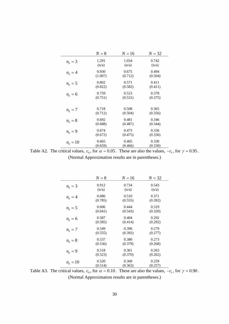
Appendix: Critical Values for the t distribution:

In this appendix, we show how to compute values for 0c and 1c through Monte Carlo

simulation or with a normal approximation. Let the cdf of the distribution of the average of N

independent standard t-distributed random variables each with 0 1n − degrees of freedom be

called ( )0, 1,t N n x− , where x is the argument of the cdf. Let 0c be the 1-α quantile of this

distribution and 1c be the 1-γ quantile of this distribution. Values for 0c and 1c for some common

values of α, γ, 0n and N are given in Tables A1, A2, and A3.

Monte Carlo Simulation to determine 0c and 1c for ( )0, 1,t N n x− .

1. Generate a set of N random variables, {1, }it i N∀ ∈ , from a central t-

distribution with 0 1n − degrees of freedom and compute the average, called

1

1 N

j ii

t tN =

= ∑ .

2. Choose a large number, M, and repeat Step 1 M times to obtain the average of

each set, {1, }jt j M∀ ∈ .

3. Rank order the jt ’s so that ( ) ( )j kt t j k> ∀ > to obtain ( ) {1, }jt j M∀ ∈ .

4. Let [ ]0 (1 )j Round Mα= − and [ ]1 (1 )j Round Mγ= − , then ( )00 jc t= and

( )11 jc t= , where [ ]Round x rounds x to the nearest integer.

Normal Approximation to determine 0c and 1c for ( )0, 1,t N n x− .

The variance of a t-distribution with v degrees of freedom is 2

vv −

for 2v > . If N is

relatively large, then by the central limit theorem, the average of N independent t-distributed

29

random variables is approximately normal with variance ( )2

vN v −

. Thus,

( ) ( )10 1

2vc

N vφ α−≈ −

− and

( ) ( )11 1

2vc

N vφ γ−≈ −

−, where ( )1 xφ − is the inverse function

for the standard normal distribution.

In Tables A1, A2, and A3, critical values 0c and 1c calculated by Monte Carlo simulation

(and the normal approximation) are presented for cases where the normal approximation is not

very accurate. For 32N > , the normal approximation is reasonably accurate and thus tables are

not necessary. Notice that if ( )1 γ α− = , then 1 0c c= − . The normal approximation cannot be

used when 0 3n = since there is no closed form for the variance of the t-distribution with 2

degrees of freedom.

8N = 16N = 32N =

0 3n = 2.626 (n/a)

1.885 (n/a)

1.426 (n/a)

0 4n = 1.523 (1.425)

1.098 (1.007)

0.758 (0.712)

0 5n = 1.200 (1.163)

0.848 (0.822)

0.603 (0.582)

0 6n = 1.103 (1.062)

0.737 (0.751)

0.536 (0.531)

0 7n = 1.017 (1.007)

0.726 (0.712)

0.517 (0.504)

0 8n = 1.001 (0.973)

0.712 (0.688)

0.507 (0.487)

0 9n = 0.953 (0.950)

0.668 (0.672)

0.483 (0.475)

0 10n = 0.965 (0.933)

0.676 (0.659)

0.473 (0.466)

Table A1. The critical values, 0c , for 0.01α = . These are also the values, 1c− , for 0.99γ = . (Normal Approximation results are in parentheses.)

30

8N = 16N = 32N =

0 3n = 1.291 (n/a)

1.034 (n/a)

0.742 (n/a)

0 4n = 0.930 (1.007)

0.675 (0.712)

0.494 (0.504)

0 5n = 0.802 (0.822)

0.571 (0.582)

0.411 (0.411)

0 6n = 0.759 (0.751)

0.523 (0.531)

0.378 (0.375)

0 7n = 0.718 (0.712)

0.508 (0.504)

0.365 (0.356)

0 8n = 0.692 (0.688)

0.481 (0.487)

0.346 (0.344)

0 9n = 0.674 (0.672)

0.473 (0.475)

0.336 (0.336)

0 10n = 0.665 (0.659)

0.465 (0.466)

0.330 (0.330)


8N = 16N = 32N =

0 3n = 0.912 (n/a)

0.734 (n/a)

0.543 (n/a)

0 4n = 0.686 (0.785)

0.510 (0.555)

0.371 (0.392)

0 5n = 0.606 (0.641)

0.444 (0.543)

0.319 (0.320)

0 6n = 0.587 (0.585)

0.404 (0.414)

0.292 (0.292)

0 7n = 0.549 (0.555)

0.396 (0.392)

0.279 (0.277)

0 8n = 0.537 (0.536)

0.380 (0.379)

0.273 (0.268)

0 9n = 0.518 (0.523)

0.361 (0.370)

0.263 (0.262)

0 10n = 0.520 (0.514)

0.360 (0.363)

0.259 (0.257)


31

Acknowledgement

Dr. Ankenman’s work was partially supported by EPSRC Grant GR/S91673 and was undertaken

while Dr. Ankenman was visiting Southampton Statistical Sciences Research Institute at the

University of Southampton in the UK. Dr. Wan’s research was partially supported by Purdue

research Foundation (Award No. 6904062). We would also like to thank Russell Cheng, Sue

Lewis, Barry Nelson, and an anonymous referee for many helpful discussions and comments.

References Banks, J.; Carson II, J. S.; Nelson, B. L.; and Nicol, D. M. (2005). Discrete-Event System

Simulation. Fourth Edition, Prentice Hall, New Jersey.

Bettonvil, B. and Kleijnen, J. P. C. (1997). “Searching for Important Factors in Simulation

Models with many Factors: Sequential Bifurcation”. European Journal of Operational

Research 96, pp. 180-194.

Bishop, T. A. and Dudewicz, E. J. (1978). “Exact Analysis of Variance with Unequal Variances

– Test Procedures and Tables”. Technometrics 20, pp. 419-430.

Bishop, T. A. and Dudewicz, E. J. (1981). “Heteroscedastic ANOVA”. Sankhya 20, pp. 40-57.

Dean, A. M. and Lewis, S. M., eds. (2005). Screening: Methods for Experimentation in Industry

. Springer-Verlag, New York.

Kuhfeld, W. F. and R. D. Tobias, R. D., (2005)., “Large Factorial Designs for Product

Engineering and Marketing Research Applications”., Technometrics 47, pp. 132-141.

Lewis, S. M. and Dean, A. M. (2001). “Detection of Interactions in Experiments with Large

Numbers of Factors (with discussion).”. J. R. Statist. Soc. B 63, pp. 633-672.

32

Lu, X. and Wu, X. (2004) “A Strategy of Searching for Active Factors in Supersaturated

Screening Experiments”. Journal of Quality Technology 36, pp. 392-399.

Montgomery, D. C. (2001). The Design and Analysis of Experiments, Fifth Edition, Wiley, 2001.

Santner, T. J.; Williams, B.; and Notz, W. (2003). The Design and Analysis of Computer

Experiments. Springer-Verlag, New York.

Stein, C. (1945). “A Two Sample Test for a Linear Hypothesis whose Power is Independent of

the Variance”. Annals of Mathematical Statistics 16, pp. 243-258.

Wan, H.; Ankenman, B. E.; and Nelson, B. L. (2005a). “Controlled Sequential Bifurcation: A

New Factor-Screening Method for Discrete-Event Simulation”. Operations Research, to

appear.

Wan, H.; Ankenman, B. E.; and Nelson, B. L. (2005b). “Simulation Factor Screening With

Controlled Sequential Bifurcation in the Presence of Interactions”. Working Paper,

Department of Industrial Engineering and Management Sciences, Northwestern University,

Evanston, IL.

Wu, J. C. F. and Hamada, M. (2000). Experiments: Planning, Analysis and Parameter Design

Optimization. Wiley, New York.

two-stage controlled fractional factorial screening for...

Documents