two approaches to solving a numerical general equilibrium

32

TWO APPROACHES TO SOLVING A NUMERICAL GENERAL EQUILIBRIUM MODEL

* Hidetaka Kawano

1. INTRODUCTION

The main objective in making a numerical general equilibrium model empirically operational

is to develop an easily implementable algorithm which is fast and efficient. This paper

compares the performance of two approaches to solving a numerical general equilibrium

model. The alternative approaches are (1) the single equation approach with a factor price

revision rule (FPRR), and (2) the sub-model approach with a factor price-quantity revision

rule (FPQRR). The sub-model approach with the FPQRR turns out to be the more

promising choice for solving a large-scale empirical general equilibrium model.

The single equation approach for a simple illustrative general equilibrium model is set

out by Shoven and Whalley (pp. 43-44, 1992). The main feature of this approach is to

reduce the dimensionality of solution space to the number of factors of production. In

other words, the equilibria for the illustrative two-good-two-factor model are characterized

by two excess factor demand functions for both capital and labor. Due to Walras' law, the

entire general equilibrium system is further collapsed to a single excess factor demand

equation. Any root finding algorithm such as Bisection, Newton-Raphson, or any other

efficient fixed point algorithms can be applied. However, to find a root of the single

equation, the iterative Kimbell-Harrison FPRR (1986) was used, with some modifications,

by simply assuming that the weighted average of the elasticities of substitution proposed by

Kimbell and Harrison (1986) is equal to unity. This simple FPRR was applied successfully

to the single equation approach to solve the simple illustrative model.

The sub-model approach for a general equilibrium model is what is also called "a partial

equilibrium approach" by Damus (1993) who programmed in BASIC. To find equilibrium

factor prices, he revised not only factor prices but also quantities in iterative processes.

This approach suggests Damus' revising rule as a factor price-quantity revision rule

(FPQRR) in contrast to the factor price revision rule (FPRR) proposed by Kimbell

Harrison (1986). Reprogramming the Damus model in C-Ianguage (C) with some minor

modifications, the reliability of his sub-model approach with the FPQRR was confirmed.

The overview of the programming structure is that the system consists of two separate sub-* Aomori Public College

models. Each sub-model has a separate solution, on the assumption that a solution derived

from one sub-model is considered exogenous to the other sub-model. A general

equilibrium is achieved when and if the solutions in both sub-models are mutually

consistent with each other. When the joint equilibrium solution is found, this economic

system is in equilibrium where all producers and consumers optimize their respective

objective functions subject to their respective constraints.

The main weaknesses of the single equation approach are: (1) the entire system is a

"solid" block which is too rigid and tedious to modify for a number of particular

applications from a programming standpoint, and (2) the time for detecting and removing

programming errors is significantly increased, especially when the dimensionality of

solution space is large. Because of these weaknesses, this approach is not practical for a

large scale model. However, the difficulties of the single equation approach mentioned

above do not imply the impracticability of the FPRR for other applications.

On the other hand, the main strengths of the sub-model approach in comparison with the

single equation approach are: (1) the overall programming structure of the model is easily

learned and modified by replacing some sub-models with alternatives; (2) the interrelated

mechanics between the factor market and the goods market sub-routines in a general

equilibrium setting is more clearly observed; (3) each sub-model can be tested separately

so that it considerably reduces the time for detecting and removing programming errors;

and (4) equilibrium solutions can be easily computed even when the model structure

becomes larger. The possible weakness is that the number of iterations is relatively

increased till convergence occurs. However, this weakness no longer poses a serious

problem because of the recent rapid technological advancement in computing. Because of

these strengths, the sub-model approach with the FPQRR would be a good choice as a

general algorithm for solving a larger scale empirical general equilibrium model.

In section 2, the general structure of the model is specified. In sections 3 and 4, the

single equation approach with the FPRR and the sub-model approach with the FPQRR are

described. In section 5, uniqueness and global stability for the illustrative model are

discussed. Some applications of the sub-model approach are discussed in section 6. The

conclusion follows in section 7. All notations are defined as they appear for the first time

in the text.

33

2. THE GENERAL STRUCTURE OF THE MODEL

2.1. The mainfeature a/the model

A simplified numerical general equilibrium model is presented to illustrate how each

solution technique is used. I) This model is structurally representative of many other large

scale empirical models actually in use for policy analyses. This simplified model has two

final goods (good 1 and good 2), two factors of production (capital K and labor L), and two

classes of consumers (rich and poor classes). A "'rich" consumer group (R) owns all the

capital in the economy. A "poor" group (P) owns all the labor in the economy. On the

production side, production technology in each sector is represented by a constant-returns

to-scale, constant-elasticity-of-substitution (CES) production function. Each factor demand

function is derived from a cost minimization problem subject to given technology and

given output level. All consumer preferences are represented by a constant-elasticity-of

substitution (CES) utility function. Each commodity demand function is derived from a

utility maximization problem subject to the budget constraint faced by each consumer

class. There are four exogenous variables: the household endowments of labor and capital

(Krn

and Lm). There are twelve endogenous variables for the required conditions for

equilibrium: (1) four prices (pj, P2 , W, r), and (2) four commodities demanded (xt ,X{ ,X2R

, X{), and (3) four factors demanded (KJ, K2, LJ, L2)' The solution to the model

characterized by the twelve endogenous variables must satisfy the equilibrium conditions

in the model: (1) excess demand conditions for all goods and factors, and (2) zero-profit

conditions in each industry. In addition, all market demand functions for goods and factors

are continuous, non-negative, homogenous of degree zero in their respective prices and

must satisfy Walras' Law for theoretical consistency. Only relative prices are significant in

affecting economic agents' decisions in general equilibrium models so that wage rate w is

chosen as numeraire.

2.2. The demand side a/the model

There are two consumers, one rich (R) and the other poor (P), in the economy. Both

consumers maximize their own utilities by solving the following constrained maximization:

Max[xt, xt ~ 0] Um

( xt, X2m

)

~ Xm == ym s.t. L- Pi i

(1)

iEI

1) This simplified structure of a numerical general equilibrium model was taken from Shaven and Whalley (1984).

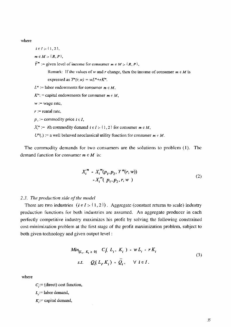
where

i E I := f 1 , 2 },

m EM := {R, P } ,

ym := given level of income for consumer m EM == {R, P},

Remark: If the values of w and r change, then the income of consumer m E M is

expressed as P'(r, w) = wLm+r/(!".

Lm := labor endowments for consumer m EM,

/(!/: = capital endowments for consumer m E M,

w := wage rate,

r := rental rate,

p; := commodity price i E I,

x;m:= ith commodity demand i E I := { 1 , 2 } for consumer m E M,

U"(.) := a well behaved neoclassical utility function for consumer m EM.

The commodity demands for two consumers are the solutions to problem (1). The

demand function for consumer m E Mis:

X;m = X;m(pl'P2' ym(r, w» =Xjm( Pl'P2' r, w )

2.3. The production side o/the model

(2)

There are two industries (i E I == { 1 , 2 }). Aggregate (constant returns to scale) industry

production functions for both industries are assumed. An aggregate producer in each

perfectly competitive industry maximizes his profit by solving the following constrained

cost-minimization problem at the first stage of the profit maximization problem, subject to

both given technology and given output level:

where

Min[L K 0] C,.( L,., K,. ) = w L,. + r K ,. I' I:?!:

s.t.

Ct:= ( direct) cost function,

L/:= labor demand,

K/:= capital demand,

\if i EI.

(3)

35

Q;:= given output level,

Q;('):= A well behaved neoclassical (strictly quasiconcave) production function for the j

aggregate industry production function i E I.

-The derived factor (labor and capital) demands for given output level Qi are:

(4)

At the second stage of the profit maximization problem, the factor demand functions as output

changes to maximize the profit under each perfectly competitive industry are given as :

(5)

2.4. Excess demand conditions

Excess demand conditions for both goods and factors are :

L xt( PI ,P2' r, w ) - Q; ~ 0 ViE I. mEM

(6) iEI mEM

L Ki (Qi I r, w) - L K m ~ O. iEI m EM

2.5. Zero-profit conditions

If the output of industry i is positive, the price of output i is equal to the long run average

costs (zero-profit in the long run) under perfect competition.

where

Pi (r, w) = w Ii (11 r, w ) + r Ki (Ilr, w ),

I, ( 11 r, w) : ~,' k, (11 r, w) : ~>

(7)

\if i EI.

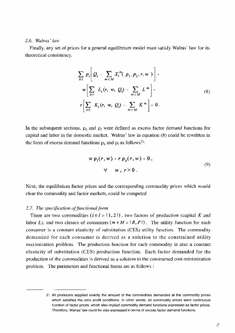
2.6. Walras'law

Finally, any set of prices for a general equilibrium model must satisfy Walras' law for its

theoretical consistency.

L Pi[Qi - L xt( Pl'P2' r, w ) 1 + iEI m EM

W[L L;(r, w, Qi) - L L m] +

~ mEM (8)

r[L Ki(r, w, Qi) - L Km] = o. iEI m EM

In the subsequent sections, Pk and PI were defined as excess factor demand functions for

capital and labor in the domestic market. Walras' law in equation (8) could be rewritten in

the form of excess demand functions P k and PI as follows2}:

w plr, w) + r Pk(r, w) = 0, (9)

v W, r>O.

Next, the equilibrium factor prices and the corresponding commodity prices which would

clear the commodity and factor markets, could be computed

2.7. The specification of functional form

There are two commodities (i E I := { 1 , 2 }) , two factors of production (capital K and

labor L), and two classes of consumers (m E M := {R, P }). The utility function for each

consumer is a constant elasticity of substitution (CES) utility function. The commodity

demanded for each consumer is derived as a solution to the constrained utility

maximization problem. The production function for each commodity is also a constant

elasticity of substitution (CES) production function. Each factor demanded for the

production of the commodities is derived as a solution to the constrained cost-minimization

problem. The parameters and functional forms are as follows :

2) All producers supplied exactly the amount of the commodities demanded at the commodity prices which satisfied the zero profit conditions. In other words, all commodity prices were continuous

function of factor prices, which also implied commodity demand functions expressed as factor prices.

Therefore, Walras' law could be also expressed in terms of excess factor demand functions.

37

38

On the demand side

( 1) CES utility functions :

U m = (~ «(X~ )lIpm(X;m ipm-I)lpm) pm/(pm_l)

lEI

'V m EM. where

a.~:= consumer share parameters for Xi. ViE I, and V m EM,

pm:= elasticities of substitution in consumption for XI. ViE I, and V m EM.

(2) Demand functions:

where

xt = pm ~ m (1- p",>

Pi L- (Xi Pi iEI

'VmEM,A'ViE!.

Lm:= household labor endowments for m EM,

Km := household capital endowments for m EM.

On the supply side

(1) CES production functions:

Q i = 'P i (Oi (L)(al

- I)lal

+ (1 _ Oi) (K) (al

- 1)/a I) ail (al

- I)

'ViE!. where

'P 1:= parameters for scale factors for i E I,

(,1:= factor weighting parameters for i E I,

a ':= elasticities of substitution between factor inputs K. and L. for i E I. I I

(2) Factor demand functions:

'ViE!.

(10)

(11)

(12)

(13)

2.8. Specification of parameters

In this simple model, there are twelve parameter values that need to be specified: (1) six

production function parameters for two commodities supplied by two industries (<1>', 8,and

for i E I), and (2) six utility function parameters for two commodities demanded by two

consumer groups (a; and (r for i E I, and for m EM). There are four exogenous variables:

the endowment of labor and capital (K and Lm

, V m E M) for each of two consumers. All

specified parameter values are summarized in table 1.

Table 1

Specification of parameters for a simple general equilibrium model

Commodity 1 Commodity 2

Rich Consumers R

112

0.5

Rich households Poor households

Production Parameters

Demand Parameters

Endowments

'PI

1.5 2.0

p 111

0.3

6; 0 1

0.6 2.0 0.7 0.5

Poor Consumers p pp

112

0.7 0.75

LK1IIEM LL1IIEM

25 0 0 60

3. THE SINGLE EQUATION APPROACH WITH FACTOR PRICE REVISION

The single equation approach with a simple factor price revision rule (FPRR) is

presented in this section. This single equation type of the computational solution procedure

for a simple general equilibrium model is also set out by Shoven and Whalley (pp. 43-44,

1992). The procedure is to reduce the dimensionality of solution space to the number of

factors of production. In other words, the equilibria for this two-good-two-factor model are

characterized by two excess factor demand functions for both capital and labor. Wage rate

is considered as a numeraire, since relative prices are important in a general equilibrium

setting. Due to Walras' law, the entire general equilibrium system is collapsed to a single

equation to solve for the optimal rental rate r*. To find a root r* of the single equation, the

39

40

Kimbell-Harrison FPRR (1986) is simplified by assuming that the weighted average of the

elasticities of substitution proposed by Kimbell and Harrison (1986) is equal to unity. This

simple FPRR is then applied to the single equation approach to solve the general

equilibrium model. 3) As noted by Kimbell and Harrison (1986), the FPRR is a simple form

of Walrasian tatonnement process that raises the price of a factor in excess demand and

lowers the price of a factor in excess supply.4) The specific solution procedure is as

follows:

Step 1: Assign the arbitrarily chosen initial value to wage rate r (r > 0 ).

Step 2: Determine factor demands per unit of output i, since factor demand functions Li

and Ki are derived as a solution to constrained cost-minimization problem (3).

Factor demand functions per unit of output i are:

(14)

Step 3: Compute commodity prices Pi using the conditions that the price of output i is

equal to long run average costs (zero-profit conditions).

(15) 'r;f iEI.

Step 4: Compute individual commodity demands (X]R, X/, X/, X/) since commodity prices

(PiEl ) are computed in step 3.

Demand functions are:

3) In this single equation approach, any good choice of algorithm to locate roots of equations, such as

Bisection method, many Newton and Secant method varieties, etc. (Tanaka and Kawano, 1996), can

be applied to find any real number root r* for whichf(r*) =0.

4) Samuelson (1947) formulated the simultaneous Walrasian tatonnement process in the form of a set

of differential equations, to describe the price changes of each commodity in proportion to its excess

demand at any time (Arrow and Hurwicz, 1958).

I}m " m (I-I}"') Pi L.J a i Pi

iEI

\/mEM,l\iEI.

(16)

Step 5: Compute the market demands for two commodities by two consumers, and then

compute the output of commodities through the market clearing condition for two

commodity markets.

\/ tEl. (17)

Step 6 : Compute factor demand functions Li and Ki through (9).

Li(r,w)=li(r,w)*Qi(r,w) \/ tEl. (18)

Ki ( r, w ) = ki( r, w ) * Ql r, w ) \/ i E I.

Step 7: Find the converged equilibrium value r* of a variable parameter r in both excess

factor demand functions, Pk for capital Kie/ and PI for labor L iei' Either one of two

excess factor demand functions can be dropped due to Walras' law, which guarantees that

the value of the sum of all excess factor demand functions is zero. The excess labor

demand function PI is dropped in this computation. Therefore, this entire general

equilibrium system is reduced to one equation to solve, given an initial value for a variable

parameter r by treating the wage rate w as a numeraire. Better approximations of the

equilibrium value r* with increased accuracy are gained if the converging value for Pk is

closed to zero.

Pk (r I w = 1 ) = L Ki (r, w) - L K m . (19) iEI mEM

Step 8: Set up the crucial procedure for revising factor prices over iterations. This factor

price revising procedure turns out to be a special case of the Kimbell-Harrison FPRR

(1986). The weighted average of the elasticities of substitution in production for all

industries in the model is considered unity in my specification. The converged value r* is

gained through a finite number of iterations for each computational experiment. The

number of iterations performed for each experiment in appendix A is approximately forty.

This simple formulation without the weighted average of the elasticities of substitution

41

42

performed extremely well. The formulation for revising a factor price r is specified as:

where

r - r _,_'EI __

[ E Ki 1

n+l - n E K m '

rn:= finite n-th iterated factor price r, 2

L K;:= total demand for capital, /-) p

L K m := total supply for capital. moR

mEM n

(20)

This formulation of Walrasian tatonnement process is numerically much easier to solve

than Samuelson's specification of the t.Honnement process in the form of a set of

differential equations. The equilibrium factor price r* is achieved when a factor demand

and supply are equated at a specified level of tolerance.

Step 9: Specify the level of tolerance for the relative error form of the capital market

clearing condition to be satisfied.

The relative error form of the condition is specified as:

>Tolerance = 1.0e-15 . (21)

Step 10: Repeat the entire process from steps 2 to 9 and keep revising the finite n-th iterated

factor price rn until its convergence occurs with the above condition in step 9 satisfied.

4. THE SUB-MODEL APPROACH WITH FACTOR PRICE-QUANTITY REVISION

The second solution procedure for a general equilibrium model is what is also called "a

partial equilibrium approach" by Damus (1993) who programmed this approach in BASIC.

In fact, he used the factor price-quantity revision rule (FPQRR) to find a solution to the

model. In this rule, both factor price and quantity are revised in an iterative approach. The

Damus model was reprogrammed in C-Ianguage with some modifications verifying the

reliability of the sub-model approach with the FPQRR.5)

In this approach, the entire system consists of two sub-models: 1) a factor market sub

model and 2) a goods market sub-model. Each sub-model has a separate solution on the

assumption that a solution derived from one sub-model is considered exogenous to the

other sub-model. A general equilibrium is achieved when the solutions in both sub-models

are mutually consistent with each other. In other words, the two sub-models can be tested

and solved separately to make sure if each sub-model is logically consistent as well as

computationally feasible beforehand. The next step is to compute a joint equilibrium

solution of the entire general equilibrium system which is comprised of the two sub

models. At the joint equilibrium solution, this economic system is in equilibrium where all

producers and consumers optimize their respective objective functions subject to their

respective (technical as well as financial) constraints. The general structure of the sub

model approach to a general equilibrium computation is illustrated in Figure 1.

Figure 1

General Equilibrium Computation

Iterflle until mutually consistent solutions to each sub-model lire gained III

--~-~-~ CExDpuJus Initilll Values J Steps 1-5 t I

I_M_~_

Steps 6-9 .. The solutions to the above sub-routine fire fed.

\ Goods markets must clear .

I

-~

Goods MIII'kd Sub-Routine !

I

SUps IIHl t The __ t. the...". ,.6-<o""e .,.., ...

The specific solution procedure is as follows:

Step 1: Assign arbitrarily given initial values to Kl (O<Kl<K) and r (r>O) for the

subsequent iterations. The wage rate w is treated as a numeraire throughout the entire

solution procedure.

5) The illustrative model structure was taken from Shaven and Whally (1984, and pp. 45-47, 1992).

43

44

Step 2: Find the value of K2 (K2>O).

(22)

Step 3: Find the valueof L l , and L2•

(3-1) Marginal rate of technical substitution for goods 1 (MATS l ) is equal to that of good 2

(MATS2) along the contract curve in the two-factor Edgeworth box, given rand w.

r MRTS. =-, , w \;fiEf. (23)

(3-2) Since a constant elasticities of substitution (CES) production function is assumed,

marginal rate of technical substitution for goods i is derived as:

dL. MRTS. == - --' =

, dK. , 1 - t> i ( L i) ;1

f>i K. ' , \;f i E f. (24)

(3-3) By equations (23) and (24), Li is expressed as:

(

• ) 1 0' r a L.= --- K.,

, 1 - f>i W ' \;f i E f. (25)

Step 4: Revise the initially given value of rental rate r and check if the labor market _ 2

clearing condition L - L L; '" 0 is approximated at the specified level of tolerance. A ;·1

modified Kimbell-Harrison (1986) factor price revision approach is used for revising a

factor price r.6)

(26)

where

L LI:= total demand for labor, lEi

i = L L m := total (economywide) endowment for labor. mEM

6) As discussed before, the weighted average of the elasticities of substitution used by Kimbell and

Harrison (1986) in production for all industries is considered unity in this specification.

As noted by Kimbell and Harrison (1986), this factor revision rule is a simple form of the

Walrasian tatonnement process that raises the price of a factor in excess demand and lowers

the price of a factor in excess supply. The equilibrium rental rate r* is achieved when a

labor market clearing condition is satisfied at a specified level of tolerance.

The absolute error form of the labor market clearing condition is converted into the

relative error form in revising a factor price r in equation (26), since the relative error form

is desired for the accuracy of an approximation in general. 7) The level of tolerance for

approximation is also specified as 1.0e-15. The relative error condition imposed for factor

price revision is now formulated as:

> tolerance = 1.0e-15. (27)

Step 5: Repeat the entire process from Step 1 to Step 5 and keep revising the finite n-th

iterated factor price rn formulated in equation (28) as long as the relative error condition in

equation (27) is satisfied. As soon as it is not satisfied through the repeated iterations, the

finite n-th iterated factor price r n is approximately converged at the specified level of

tolerance. It is the converged rental rate r* that clears the labor market for initially given K j •

( -) L r

n L Lj

iEI n

(28)

Up to Step 5, the finite n-th iterated factor price rn is converged for the initial value of K,

given in Step 1. When this initially assigned value for K j is revised, the converged factor

price rn changes correspondingly. Thus, a group of steps 1-5 forms a complete labor

market sub-model, given exogenously the initial value for K j •

Step 6: Find outputs Q, and Q2 through a CES production function assumed for each good.

\;fiE!. (29)

7) In Higham (p.5, 1996) the relative error is desired for the accuracy of an approximation. The relative

error is a more precise measure and is base independent. An estimate or bound for the relative error

should be provided whenever an approximate answer to a problem is found.

45

46

Step 7: Find final goods prices PI and P2 through the zero-profit conditions.

r K; + w L; P;=---

Q; 'ifiEI.

Step 8: Find household incomes for the rich (R) and the poor (P).

where

ym=wLm+rK m, 'if mE M.

L "':= the endowment oflabor for household m EM,

K Iff:= the endowment of capital for household m EM.

(30)

(31)

Step 9: Find goods demands xt through a CES utility function assumed for each good.

mym (X; X.m = ______ _

I pm Pi L

iEI

'ifiEI,A'ifmEm. (32)

A block of steps 6-9 specifies supply and demand functions for each goods market, and all

goods markets must clear. This block of steps forms a complete labor market sub-model,

given exogenously the initial value for K 1•

Step 10: Revise the exogenously given initial value for KI such that all goods markets

must clear, because the initially given KI does not necessarily clear all the goods markets.

This is a final block of steps to execute the recursive general equilibrium loops to iterate

steps 1-10 until a mutually consistent solution to each sub-model is found.

(10-1) Specify the level of tolerance for the relative error form of the goods market

clearing condition.

L L X;m - Q; mEM ;EI > tolerance = l.Oe-lS. (33)

(10-2) Iterate the entire procedure "in the most outer loop" from steps 1-10 to revise Kl as

long as the above condition is satisfied at the specified level of tolerance.

(34)

Equation (34) must be satisfied to show that the goods market is in equilibrium.

( -) K -K K 1,n~I - I,n ~ Ki

lEI n

(35)

Equation (35) must be satisfied to show that capital KiEI are fully employed in both sectors.

5. UNIQUENESS AND GLOBAL STABILITY

5.1. Uniqueness

For theoretical consistency, it was crucial to investigate the uniqueness and the stability

of the equilibrium in the Walrasian tatonnement process. Instead of the formal axiomatic

analyses, a computational approach to this issue can be employed. Although a numerical

computational approach is not a rigorous proof, it can be considered a close approximation

to a formal axiomatic analysis. However, the computational approach has made it possible

to explore more intuitively the questions of global stability and uniqueness of the

equilibrium vector, by explicitly solving the highly non-linear equations of the general

equilibrium model. This was possible due to both recent technical advancements in

computer technology and refinements in operational algorithms. Of course, all necessary

properties such as homogeneity, Walras' law, continuity, and other excess factor demand

functions were assumed to be satisfied. First, the question of uniqueness was considered in

this section and then followed by the question of global stability in section 4.2. Both

uniqueness and global stability properties for the model were essential in order to derive

the reliable simulation results under investigation. For the ease of exposition, I used the

single equation approach with the factor price revision rule (FPRR) for solving the

benchmark model.

Arrow, Block, and Hurwicz (1959) obtained a major analytical result on the stability of a

general equilibrium model. For a two primary input economy, Arrow and Hahn (pp.238-

40, 1971) stated a necessary and sufficient condition that W* was the unique equilibrium,

with the assumptions of constant returns to scale and no joint production. That was

W*S(W)<O, for all W¢W* and W>>O where W was the vector of factor prices, and S(.) was

the vector of excess factor supply functions. If Z(.) was assumed to be the vector of excess

47

48

factor demand functions ( Z(.) = -S(.) ), then the condition is equivalently stated,

w*Z(W) >0. This condition also implied that the two inputs were gross substitutes, which

meant that the Jacobian matrix of excess factor demand functions had all positive off

diagonal terms. The necessary and sufficient condition that W* be the unique equilibrium

was computationally checked with the benchmark model.

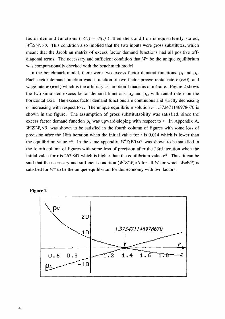
In the benchmark model, there were two excess factor demand functions, Pk and PL'

Each factor demand function was a function of two factor prices: rental rate r (r>O) , and

wage rate w (w= 1) which is the arbitrary assumption I made as numeraire. Figure 2 shows

the two simulated excess factor demand functions, PK and PL> with rental rate r on the

horizontal axis. The excess factor demand functions are continuous and strictly decreasing

or increasing with respect to r. The unique equilibrium solution r=1.373471146978670 is

shown in the figure. The assumption of gross substitutability was satisfied, since the

excess factor demand function PL was upward-sloping with respect to r. In Appendix A,

w*Z(W»O was shown to be satisfied in the fourth column of figures with some loss of

precision after the 18th iteration when the initial value for r is 0.014 which is lower than

the equilibrium value r*. In the same appendix, W*Z(W»O was shown to be satisfied in

the fourth column of figures with some loss of precision after the 23rd iteration when the

initial value for r is 267.847 which is higher than the equilibrium value r*. Thus, it can be

said that the necessary and sufficient condition (W*Z(W»O for all W for which W~W*) is

satisfied for W* to be the unique equilibrium for this economy with two factors.

Figure 2

20

1.373471146978670 r

0.6 0.8

-10

5.2. Global stability

The problem of the global stability of the dynamic behavior of the factor prices resulting

from the tatonnement of the Walrasian auctioneer in the factor market was computationally

approached and analyzed along the lines of Arrow and Hahn (pp.270-75, 1971). There can

be many limit points resulting from the many different solution paths generated by the

differential equations of the Walrasian auctioneer's rule, depending on the choice of initial

conditions. If there were multiple equilibria, no equilibrium could be claimed to be

globally stable. Although a number of equations involved in this general equilibrium

model were of a highly non-linear nature, due to rapid technological advancements in

computing the computations of the model no longer posed a grave problem in actually

solving a set of equations to investigate the above stability questions. In the actual

computation, two approaches were used: 1) the single equation approach with the FPRR

and 2) the sub-model approach with the FPQRR, instead of solving the set of differential

equations with respect to a time variable. In both approaches, the computations were

executed within a second till convergence occurred at the specified level of tolerance,

regardless of the initial values assigned. In both approaches, I set the tolerance level (for

the relative error form of the condition to be satisfied) in high precision (1.0e-15). Thus,

both computational rules and the unique equilibrium could be claimed to be globally stable.

These numerical exercises were not a proof, but they were useful approximations to other

formal axiomatic deductions, especially when the dimensions of a model increased.

6. SOME APPLICATIONS OF THE SUB-MODEL APPROACH

The main strengths of the sub-model approach in comparison with the single equation

approach are: (I) the overall programming structure of the model is easily learned and

modified by replacing some sub-models with alternatives; (2) the interrelated mechanics

between the factor market and the goods market sub-routines in a general equilibrium

setting is more clearly observed; (3) each sub-model can be tested separately so that it

considerably reduces the time for detecting and removing programming errors; and (4)

equilibrium solutions can be easily computed even when the model structure becomes

larger. Because of these strengths, in this section, I describe some of the applications of the

sub-model approach with the FPQRR to some general equilibrium models with various tax

regimes. The first application is made to the replication of the simulation results of the

model with a 50% tax on K I (capital used in sector 1) in Shoven and Whalley (1984). Its

comparison with the results of the benchmark (non-intervention) policy is also discussed.

The sub-model approach is also applied to the combined commodity and payroll tax

policies to raise the targeted tax revenue (an equal-tax-yield equilibrium simulation). The

49

50

existence of a competitive equilibrium with taxes is essential to reliable simulation results,

as proven by Shoven and Whalley (1973). Without such a sound theoretical framework, of

course, any numerical simulation of general equilibria is not persuasive and not seriously

considered for policy implications.

The illustrative numerical general equilibrium model with taxes has some additional

features built into the benchmark (non-intervention) model. For instance, the government

sector is included. This government institutional structure is assumed to be so simple that

all tax revenues are distributed to the general public (consumers) in the form of transfer

payments. In other words, there is no public provision of goods and services contemplated

in the model. There is a government constraint where tax revenue is equal to tax

expenditure. The 50% tax placed on KI is the only source of tax revenue. The 40% of the

transfer payment goes to the rich households and the remaining 60% goes to the poor

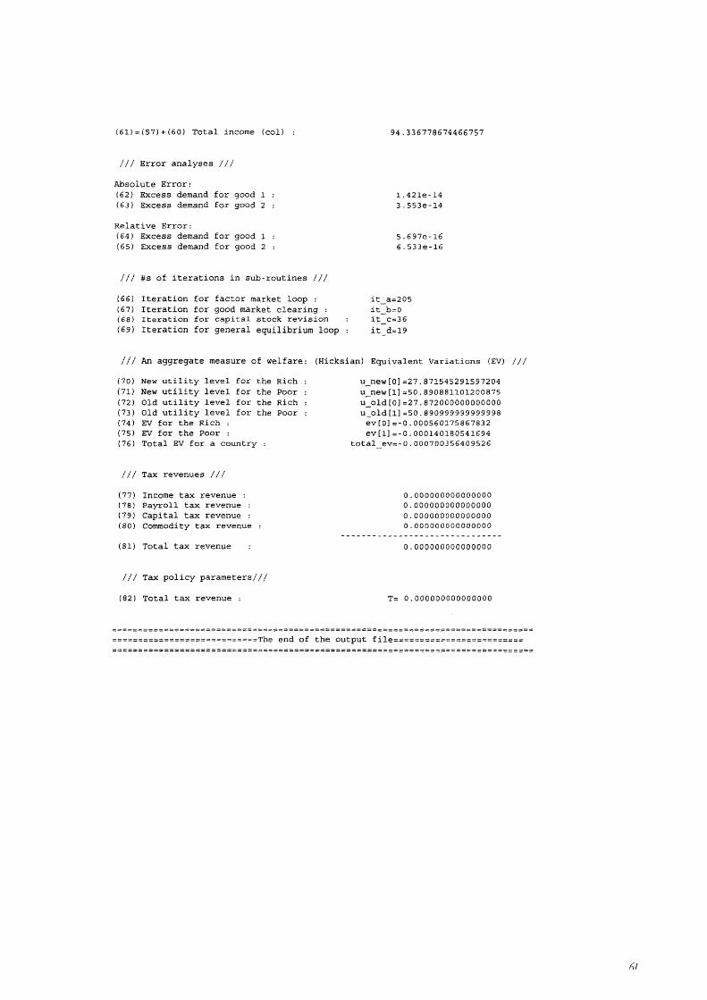
households. The equilibrium solutions are presented and compared with benchmark

equilibrium solutions in Appendix B. In Appendix C, the computational summary for the

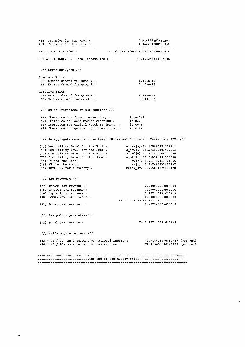
benchmark (non-intervention) general equilibrium model is reported. In Appendix D, the

computational summary for the illustrative general equilibrium model with the 50 % tax on

K 1 is provided.

For the empirical use of a numerical general equilibrium framework, refer to appendix B

and note the various effects on the general public of the 50% tax on K 1 in the simple

illustrative model. First, on the demand side of the model, the burden of the 50% tax on KI

mainly falls on the rich households, because the capital income is assumed to be the only

main source of income for the rich in the model (see Table B-3). In comparison with the no

tax case, total income for the rich is decreased. But total income for the poor is increased

after the tax imposition. Therefore, the effect of income leads to change in rich and poor

household expenditure patterns. Expenditure by the rich is decreased, while expenditure by

the poor is increased (see Table B-2). The consumption of both goods by the rich is

reduced, while the poor consumption of good 1 is reduced and the consumption of good 2

is increased (see Table B-1). Over all, the good 1 consumption is reduced and the

consumption of good 2 is increased (see Table B-l). Second, on the production side of the

model, the immediate effect of the tax on KI is the increase in the tax-inclusive per unit

cost of production in good 1 (see Table B-6). This increased per unit cost of production

leads to a decrease in production of good 1 (see Table B-4) with a less capital-intensive

method (a lower capital-labor ratio) of production as a result of employing relatively less

capital (see Table B-6). On the other hand, the tax on KI decreased the tax-inclusive per

unit cost of production in good 2 (see Table B-6). This decreased per unit cost of

production leads to an increase in production of good 2 (see Table B-4) with a more

capital-intensive method (a higher capital-labor ratio) of production as a result of

employing relatively more capital (see Table B-6). Some amount of redundant capital is

released from sector 1 to contract its production and is immediately reemployed in sector 2

to expand its production. In a general equilibrium framework, each factor and goods

market must clear at the respective coordinating equilibrium price level. It is, therefore,

absolutely important to capture the economywide general equilibrium effects for any

market intervening policy appraisal. The estimation of tax revenue is an excellent case in

point.

Finally, the numerical welfare measures of the gain or loss of any policy is firmly rooted

in microeconomics. A common procedure in applied general equilibrium models is to use

Hicksian compensating and equivalent variations associated with the equilibrium

comparison (Broadway and Bruce, 1984). In this simulation, the Hicksian equivalent

variation (EV) is used. The positive EV value implies a welfare improvement of a policy.

The welfare gain or loss of the taxes for the economy as a whole is measured by

aggregating the EVs across individuals.8) In Table B-9, the EV measure (-0.56) of the 50

% on K I tax is reported. The aggregate welfare cost of the tax is approximately 0.61 % of

the national income. However, when measured against the tax revenues, the welfare cost

of the deadweight loss is approximately 24.41 % of the tax revenues generated by the 50 %

tax on K I which turns out to be an very inefficient way of raising the revenue. In this

general equilibrium framework, the actual welfare cost of each tax policy is numerically

measured. This kind of quantitative attempt may be of considerable value to policymakers.

Finally, from a programming standpoint, the government sector is easily accommodated

in the sub-model approach with the FPQRR. This approach is also applied to the cases of

an equal-tax-yield equilibrium simulated in Tanaka and Kawano (1996), and all the

simulation results are successfully replicated within a second. In Appendix E, the

computational summary for the combined commodity and payroll tax policies is reported.9)

The EV measure of the welfare loss is 0.88 (line 76). The welfare cost of the tax is

approximately 0.66 % (line 83) of the national income. When measured against the tax

revenues, the welfare cost of the deadweight loss is approximately 2.54 % (line 84) of the

tax revenues generated by the combined commodity and payroll tax policies. These

successful applications to the various illustrative examples may indicate that the sub-model

approach with the FPQRR can be useful for solving a more large-scale empirically oriented

general equilibrium model.

8) Some aggregation difficulties are discussed in Broadway and Bruce (1984).

9) This illustrative example is taken from policy 4 in their simulation.

51

52

7. CONCLUSION

In recent years, applied general equilibrium models have been increasingly used by

researchers in various fields with a strong empirical interest in a variety of policy

questions. It is therefore necessary to develop an easily implementable algorithm which is

fast and efficient for an empirical analysis. This paper has compared the performance of

two alternative approaches: (1) the single equation approach with a factor price revision

rule (FPRR), and (2) the sub-model approach with a factor price-quantity revision rule

(FPQRR). Given the successful applications to selected general equilibrium models using

various tax regimes in the last section, the sub-model approach with the FPQRR turns out

to be the most promising choice as a general algorithm for solving a large-scale empirical

general equilibrium model. The main reasons for this choice are: (1) the overall

programming structure of the model is easily learned and modified by replacing some sub

models with alternatives; (2) the interrelated mechanics between the factor market and the

goods market sub-routines in a general equilibrium setting is more clearly observed; (3)

each sub-model can be tested separately so that it considerably reduces the time for

detecting and removing programming errors; and (4) equilibrium solutions can be easily

computed even when the model structure becomes larger.

Received: August 21, 2000

References

Arrow, K. J., H. D. Block, , and L. Hurwicz, (1959) "On the Stability of the Competitive Equilibrium, II."

Econometrica, 27 (January): pp. 32-109.

Arrow, K. J., and F. H. Hahn (1971) General competitive analysis. Amsterdam: North-Holland. Arrow, K. J., and L. Hurwicz (1958) "On the Stability of the Competitive Equilibrium, I." Econometrica 26

(October): 522-52.

Broadway, R., and N. Bruce (1984) Welfare Economics. New Nork, NY: Basil Blackwell Ltd.

Damus, S. (1993) Introduction to Applied General Equilibrium Modelling. DIA, Inc., Ottawa, Ontario,

Canada.

Higham, N. J. (1996) Accuracy and Stability of Numerical Algorithms. Philadelphia: SIAM.

Kimbell, L. J., and G. W. Harrison (1986) "On the solution of general equilibrium models." Economic

Modelling 3 (July): pp. 197-12.

Shoven, J. 8., and J. Whalley (1973) "General Equilibrium with Taxes: A Computation Procedure and an

Existence Proof." Review of Economic Studies 40,475-90.

Shoven, J. B., and J. Whalley (1984) "Applied General Equilibrium Models of Taxation and International Trade: An Introduction and Survey." Journal of Economic Literature 22,1007-51.

Shoven, J. B., and J. Whalley (1992) Applying General Equilibrium. Cambridge: Cambridge University

Press.

Samuelson, P. A. (1947) Foundations of Economic Analysis. Cambridge, Mass.: Harvard University Press.

Tanaka, H, and H. Kawano (1996) "A Simple Fixed Point Algorithm for a Static General Equilibrium Model

with Tax Policies." Aomori Public College Journal of Management & Economics Vol. 2, No.1 ,pp. 68-83.

53

Appendix

APPENDIX A

The single' equation approach with factor price revision

The initial value for r • .!!..:..Jl.!!. No. r rhoK rhoL

I. 0.6296044161257026 1099.2935655212468191 -15.3901103923392153 1494.4578839103999144

2. 1,..1112094660031924 19.1233192438939135 -12.0401262469372377 14.2252009690130166

3. 1.2776479225136428 3.7445338075884482 -4.1609614127612602 0.9820477308476541

4. L..!3 822 2 2 980566527 1.1852712800533514 -1.5143593885752473 0.1135765159205060

5. 1.3604792245858124 .2.. 4157 927752638884 -0.5564231632289847 0.0146562167181526

6. 1.3686794362312891 0.1506860872493876 -0.2050052911369136 0.0019577019512308

7. .!.:.ll17034375332480 .2......2.552 357480851304 -0.0756000325489765 0.0002646737277325

8. 1.3728189650488971 0.0203310621874522 -0.0278881878912181 0.0000359394106766

9. Wll2305221439631 .2......Q..Q.74947444918836 -0.0102889273766387 0.0000048879369408

10. 1.3733823665532321 0.0027643648830304 -0.0037961102317148 0.0000006651748486

1I. 1:..:.l.Zl!3 83 90600 9293 o . 0010198188257986 -0.0014006011924437 0.0000000905399364

12. 1.3734590611840070 0.0003762561032783 -0.0005167645769433 0.0000000123247841

13. 1.3734666878006851 0.0001388213324640 - 0.0001906654169694 0.0000000016777550

14. 1.3734695017188288 JL..Q..Q.Q.Q.512192645168 -0.0000703479535851 0.0000000002283982

15. 1.3734705399429854 0.0000188978378368 -0.0000259556039062 0.0000000000311030

16. 1.3734709230065509 0.0000069725479079 -0.0000095765891395 0.0000000000042330

17. 1.3734710643418304 o . 0000025725932211 -0.0000035333819817 0.0000000000005804

18. 1. 3734711164889499 0.0000009491848925 -0.0000013036779798 0.0000000000000832

19. 1.3734711357291711 o .0000003502116082 -0.0000004810055394 - 0.0000000000000003

20. 1.3734711428280504 0.0000001292142091 -0.0000001774719891 -0.0000000000000011

2I. 1.3734711454472559 0.0000000476749262 -0.0000000654801475 -0.0000000000000119

22. 1. 3734711464136391 o .0000000175901622 -0.0000000241595721 0.0000000000000082

23. 1.3734711467701961 0.0000000064900725 -0.0000000089139292 - 0.0000000000000019

24. 1 ~Z~4711469017515 0.0000000023945796 -0.0000000032888856 0.0000000000000004

25. 1.3734711469502903 0.0000000008835039 -0.0000000012134684 -0.0000000000000013

26. 1.3734711469681993 0.0000000003259837 - 0 . 0000000004477236 0.0000000000000055

27. 1.3734711469748069 0.0000000001202736 -0.0000000001651834 0.0000000000000089

28. ;!'·F34711462772449 0.0000000000443778 -0.0000000000609504 0.0000000000000013

29. 1 F;}471.1469781444 0.0000000000163700 -0.0000000000224922 - 0.0000000000000085

30. 1.3734711469784764 0.0000000000060432 - 0.0000000000082991 o .0000000000000010

3I. 1.3734711469785987 0.0000000000022267 -0.0000000000030624 - 0.0000000000000042

32. 1. F34711469786440 0.0000000000008251 -0.0000000000011298 0.0000000000000035

33. 1.3734711469786607 0.0000000000003011 -0.0000000000004192 -0.0000000000000057

34. 1.3734711469786669 o . 0000000000001128 -0.0000000000001528 0.0000000000000022

35. 1.3734711469786691 0.00gooooOOOOO0391 -0.0000000000000497 0.0000000000000039

36. 1. ~734711469786700 0.0000000000000142 -0.0000000000000107 0.0000000000000089

37. 1.3734711469786705 0.0000000000000053 -0.0000000000000071 0.0000000000000002

p1= 1.3991106622318159 p2= 1..0930764800086183

K1= 6.2117762182084304 K2=18.7882237817915687

---------------------------2~.0000000000000000

L1=26.3655843223416433 L2=33.6344156776583603 ---- ---- ------- -- -- --------

6Q.OQQOOOOOOOOOOOOO

it_a= 0 it_b=37 it_c=38

54

The initial value for r - ll1....!ll No. r

1.. 42.3983333969677787

2. 12.2347133043612200

3. 4.9763297813671095

4. 2.6811282096464626

5. 1. 8600841486107298

6. 1.5545218583013549

7. 1.4405578906797065

8. L..198267609502414 7

9. 1.3826263494686737

10. Lll68499251904152

11. 1.3747179016515210

12. !...1.119311663543126

13. 1.3736408781258997

14. 1.3735337713511604

15. l...:1.1.ll9425293 272 8 8

16. 1.3734796721661002

17. 1. 3734742924359149

18. 1.3734723075279069

19. L.l1l!ll5751753841

20. 1.3734713049662988

2l. 1.3734712052698477

22. 1.3734711684858059

23. 1.3734711549139516

24. 1.3734711499064747

25. 1.3734711480589139

26. 1.3734711473772374

27. 1.3734711471257262

28. 1.3734711470329279

29. 1.3734711469986893

30. 1.3734711469860568

31. 1.3734711469813956

32. 1.3734711469796761

33. 1. 3734711469790417

34. 1.3734711469788070

35. 1.3734711469787206

36. 1. 3734711462786891

37. 1.3734711469786773

38. 1.3734711469786731

39. 1.3734711469786713

40. 1.3734711469786705

pl= 1.3991106622318159 p2= 1.0930764800086183

K1= 6.2117762182084304 K2=18.7882237817915687

25.0000000000000000

L1=26.3655843223416433 L2=33.6344156776583603

60.0000000000000000

it_a: 0 it_b:40 it_C=41

rhoK

-21.0426721418378655

-17.7858524592n0539

-14.8315357753556167

-11.5305941957191962

-7.6557702283845348

-4.1068342329780494

-1.8327816848162275

;;9..7339219314077292

-0.2796542651679355

-0.1044465896458275

;;9...jl387119812386132

-0.0143072134338098

..:J1..:..!!.!!52820737224968

-0.0019493227168192

~7192837055738

-0.0002653954794010

~979215472610

-0.0000361293258084

-0.0000133303110443

-0.0000049183596182

- 0.0000018146802701

-0.0000006695451944

-0.0000002470356621

-0.0000000911463793

-0.0000000336294033

-0.0000000124079120

-0.0000000045780242

-0.0000000016891146

-0.0000000006232144

-0.0000000002299396

-0.0000000000848424

-0.0000000000313012

-0.0000000000115472

-0.0000QOOOOO042695

-0.0000000000015685

-0.0000000000005755

-0.0000000000002114

-0.0000000000000773

-0.0000000000000329

-0.0000000000000142

rhoL

5636.2162866578364628 5607.3147836156904305

754.0905023151640307 729.6621471380098001

181.4595880748527748 161.0889016220199039

57.3800392930161891 41.5431008576761442

20.5261015258933170 10.0111220093088527

7.6390572577343647 1.9984389333147350

2.8490991905412102 0.3318264277351659

1.0572570294322894 0.0492364325089145

0.3910315008435177 0.0069344365058361

0.1444106069564661 0.0009562296776008

0.0533005884723714 0.0001307991987566

0.0196683824302042 0.0000178375852008

0.0072572057103244 0.0000024298562608

0.0026776693684916 0.0000003308607903

0.0009879604607868 0.0000000450446892

0.0003645191657036 0.0000000061322078

0.0001344932546345 0.0000000008348041

0.0000496227001925 0.0000000001136348

0.0000183088130754 0.0000000000154758

0.0000067552271332 0.0000000000021071

0.0000024924112694 0.0000000000002775

0.0000009196010495 0.0000000000000434

0.0000003392963563 0.0000000000000021

0.0000001251869151 -0.0000000000000071

0.0000000461890011 -0.0000000000000140

0.0000000170419092 0.0000000000000000

0.0000000062877881 0.0000000000000039

0.0000000023199505 0.0000000000000003

0.0000000008559695 0.0000000000000026

0.0000000003158220 0.0000000000000066

0.0000000001165290 0.0000000000000005

0.0000000000430020 0.0000000000000108

0.0000000000158735 0.0000000000000138

0.0000000000058549 -0.0000000000000091

0.0000000000021600 0.0000000000000057

0.0000000000007994 0.0000000000000089

0.0000000000002949 0.0000000000000045

0.0000000000001101 0.0000000000000040

0.0000000000000391 -0.0000000000000061

0.0000000000000142 -0.0000000000000053

55

56

APPENDIX B

The computational summary for the illustrative General Equilibrium Model with a 50% tax on

K] (capital used in sector 1) in comparison with a non intervention policy (benchmark model)

Note: 1) Actual computations were done in double precision. 2) A number in each bracket refers to the number in the output summary in appendices C and D. 3) The symbol ~ indicates the decreased number from the benchmark equilibrium solutions.

1) Relative prices of goods & factors (wage rate = numeraire) :

(1) Relative price of capital (rental rate) :

(2) Relative price of labor :

(3) Relative price of good 1 :

(4) Relative price of good 2 :

(5) Relative rental price:

(6) Relative price of good 1 : in terms of good 2

2) Demand side: Table B-1. Final consumer demands:

1 Goods

2

-

r= (1) 1.373

w= (2) 1.000

PI = (3) 1.399

P2 = (4) 1.093

rlw = (5) 1.373

P/P2 = (6)1.280

Rich

(20) 11.515 ~8.989

(23) 16.674 ~15.827

.... l.128

1.000

1.467

.... 1.006

.... 1.128

1.458

Final quantities demanded

Poor

(21) 13.429 .... 13.397

(24) 37.704 41.480

Table B-2. Expenditures by consumer groups at consumer prices:

Consumer groups

Rich Poor

I (26) 16.110 (29) 18.787 Goods ~13.183 19.647

2 (27) 18.227 (30) 41.213 ~15.919 41.719

Expenditure (disposable income) (28) 34.337 (31) 60.000 ~29.I02 61.366

Total

(22) 24.942 .... 22.387

(25) 54.378 57.307

Total

(32) 34.897 ""32.830

(33) 59.439 .... 57.638

(34&35) 94.337 .... 90.468

Table 8-3. Factor-endowed incomes and transfer:

Consumer groups Total

Rich Poor

Capital income (48) 37.337 (49) 0.000 (SO) 34.337 .28.191 0.000 .28.191

Income Labor income (SI) 0.000 (S2) 60.000 (S3) 60.000

0.000 60.000 60.000

Transfer (S8) 0.000 (S9) 0.000 (60) 0.000 0.911 1.366 2.277

Factor-endowed income and transfer (S4) 34.337 (55) 60.000 (56&61) 94.337 .29.102 61.366 .90.468

(including transfer) (including transfer) (including transfer)

3) Production side: Table 8-4. Final producer outputs:

Outputs

1 (18) 24.942 Goods .22.387

2 (19) 54.378 57.307

Table 8-5. Factor costs by industry:

Goods Total

1 2

Capital costs (37) 8.532 (40) 25.805 (42) 34.337 (including tax) .6.831 .23.637 .30.468

Labor costs (36) 26.366 (39) 33.634 (43) 60.000 .25.999 34.001 60.000

Total costs (38) 34.897 (41) 59.439 (44&45) 94.337 (including tax) .32.830 .57.638 .90.468

Table 8-6. Cost per unit output & Capital-labor ratio

Cost per unit output Capital-labor ratios (KlL)

1 (46) 1.399 (16) 0.236 Goods 1.467 .0.155

2 (47) 1.093 (17) 0.559 .1.006 0.616

57

4) Government side:

Table B-7. Tax revenues

Income tax revenue (77) 0.000 0.000

Payroll tax revenue (78) 0.000 0.000

Capital tax revenue (79) 0.000 2.277

Commodity tax revenue (80) 0.000 0.000

Total tax revenue = total transfer (81) 0.000 2.277

5) Welfare measures: Table B-8. Welfare measures of a 50% tax on capital in use for production of good I

Consumer groups Total

Rich Poor

Hicksian Equivalent Variations (EV) (74) "'-4.553 (75) 3.997 (76) "'-0.556

Table B-9. Total (aggregate) welfare gain or loss

As a percent of national income As a percent of tax revenue

Hicksian Equivalent Variations (83) "'-0.614 (84) "'-24.410 (EV)

58

APPENDIX C

The benchmark equilibrium solutions for the illustrative general equilibrium. model

====================================TAX POLICY 1================================

===============================Output Summary====================================

III Prices of goods & factors III

(1) Price of capital (rental rate) r= 1.373471146978670 (2) Price of labor (wage rate=numeraire) w= 1.000000000000000 (3 ) Producer price of good 1 p [0) = 1.399110662231816 (4) Producer price of good 2 p[1)= 1.093076480008618 (5) Consumer price of good 1 (1+tau[0)*p[O)= 1.399110662231816 (6) Consumer price of good 2 (1+tau[1])*p[1)= 1.093076480008618

III Relative prices of goods & factors

(7) Relative rental price (8) Relative producer price of good (9) Relative consumer price of good

III Employments of factors III

(10) labor used in good 1 (11) labor used in good 2

(12)=(10)+(11) Total Labor:

(13) Capital used in good 1 (14) Capital used in good 2

(15) = (13) + (14) Total capital

(16) Capitalilabor ratio in (17) Capitalilabor ratio in

III Quantity supplied III

(18) Good 1 produced (19) Good 2 produced

III Quantity demanded III

:

good 1 good 2

1 1

(20) Good 1 demanded by the Rich (xR1) (21) Good 1 demanded by the Poor (xP1)

III

(22)=(20)+(21)=(18) Total good 1 demanded:



r/w= 1.373471146978670 p[0]/p[1)= 1.279975086666200

1.279975086666200

L[0]=26.365584322341668 L[1)=33.634415677658389

60.000000000000057

K[O]= 6.211776218208424 K[1)=18.788223781791576

25.000000000000000

K[o)/L[O)= 0.235601689773463 K[l)/L[l)= 0.558601165004678

q[0]=24.942472866207893 q[1)=54.378170267151795

x [0] [0] =11.514649018058366 x [1] [0] =13 .427823848149515

24.942472866207879

x[O) [1) =16 .674506125408985 x[1] [1) =37.703664141742777

54.378170267151759

in terms of good 2 price

59

III Expenditures III

(26) Expenditure on good 1 by the Rich (27) Expenditure on good 2 by the Rich

(28) = (26) + (27) Expenditure by the Rich

(29) Expenditure on good 1 by the Poor (30) Expenditure on good 2 by the Poor

(3l) = (29) + (30) Expe:qditure by the Poor

(32) = (26) + (29) Expenditure on good 1 (33) = (27) + (30) Expenditure on good 2

(34) = (28) + (31) Total expenditure (row) (35) = (32) + (33) Total expenditure

III Costs III

(36) Labor Cost in good 1 (37) Capital Cost in good 1

(col)

(38)=(36)+(37) Cost incurred in good 1:


(41)=(39)+(40) Cost incurred in good 2

(42)=(37)+(40) Total capital cost (43)=(36)+(39) Total labor cost

(44)=(38)+(40) Total cost (row) (45)=(42)+(43) Total cost (col)

(46)=(3) Cost per unit of good 1 (47)=(4) Cost per unit of good 2

III Income III

(48) Capital income earned by the Rich (49) Capital income earned by the Poor

(50)=(48)+(49) Total capital income:

(51) Labor income earned by the Rich (52) Labor income earned by the Poor

(53)=(51)+(52) Total labor income:

(54)=(48)+(51) Income earned for the Rich (55)=(49)+(52) Income earned for the Poor

(56)=(54)+(55) Total income (row) :

(57)=(50)+(53) Total factor income (col)

(58) Transfer for the Rich (59) Transfer for the Poor

16.110268213022568 18.226510461444200

E[0]=34.336778674466764

18.787011516516635 41.212988483483358

E[1]=59.999999999999993

34.897279729539200 59.439498944927557

94.336778674466757 94.336778674466757

Lc[0]=26.365584322341668 Cc[Ol= 8.531695407197553

34.897279729539221

Lc[ll=33.634415677658389 Cc[1]=25.805083267269207

59.439498944927593

34.336778674466757 60.000000000000057

94.336778674466814 94.336778674466814

1.399110662231816 1.093076480008618

34.336778674466764 0.000000000000000

TCI=34.336778674466764

0.000000000000000 60.000000000000000

TLI=60.000000000000000

y[Ol=34.336778674466764 y[1]=60.000000000000000

94.336778674466757

94.336778674466757

0.000000000000000 0.000000000000000

(60) Total transfer : Total Transfer= 0.000000000000000

(61)=(57)+(60) Total income (col)

III Error analyses III

Absolute Error: (62) Excess demand for good 1 (63) Excess demand for good 2

Relative Error: (64) Excess demand for good 1 (65) Excess demand for good 2

III #s of iterations in sub-routines III

(66) Iteration for factor market loop (67) Iteration for good market clearing (68) Iteration for capital stock revision (69) Iteration for general equilibrium loop

94.336778674466757

1.421e-14 3.553e-14

5.697e-16 6.533e-16

it a=205 it_b=O it c=36 it_d=19

III An aggregate measure of welfare: (Hicksian) Equivalent variations (eV) III

(70) New utility level for the (71) New utility level for the (72) Old utility level for the (73) Old utility level for the (74) EV for the Rich :

(75) EV for the Poor :

(76) Total EV for a country

III Tax revenues III

(77) Income tax revenue (78) Payroll tax revenue : (79) Capital tax revenue : (80) Commodity tax revenue

(81) Total tax revenue

III Tax policy parameterslll

(82) Total tax revenue :

Rich Poor Rich Poor

u_new[O) =27.871545291597204 u_new[1)=50.890881101200875 u_old[O)=27.872000000000000 u_old[l) =50.890999999999998

eV[O)=-0.000560175867832 eV[1)=-0.00014018054l694

total_ev=-0.000700356409526

0.000000000000000 0.000000000000000 0.000000000000000 0.000000000000000

0.000000000000000

T= 0.000000000000000

============================The end of the output file=========================

(,7

62

APPENDIX D

The computational summary for the illustrative general equilibrium model

with a 50 % tax on K\ (capital used in sector 1)

1* getaxOO.out *1

==========================================TAX POLICY================================== ===Simpel General Equilibrium Model with 50 percent Capital Gain Tax for Commodity 1===

===============================Output Summary====================================

III Relative prices of goods & factors (wage rate=numeraire) III

(1) Price of capital (rental rate) : r= 1.127644151564157 (2) Price of labor (wage rate=numeraire) w= 1.000000000000000 (3 ) Producer price of good 1 p [0] = 1.466514918823798 (4) Producer price of good 2 p [1] = 1.005773041898722 (5) Consumer price of good 1 (l+tau[O])*p[O]= 1.466514918823798 (6) Consumer price of good 2 (l+tau[I])*p[l]= 1.005773041898722


(7) Relative rental price (8) Relative producer price of good (9) Relative consumer price of good

III Employments of factors 11/


(12)=(10)+(11) Total Labor:


(15)=(13)+(14) Total capital

(16) Capitalilabor ratio in (17) Capitalilabor ratio in




:

good 1 good 2

1 1

(20) Good 1 demanded by the Rich (xRl) (21) Good 1 demanded by the Poor (xP1)

III


r/w= 1.127644151564157 p[0]/p[1]= 1.458097262236494

1.458097262236494

L[0]=25.999018729169372 L[1]=34.000981270830614

59.999999999999986

K[O]= 4.038757495388934 K[1]=20.961242504611068

25.000000000000000

K[Ol/L[O]= 0.155342689563037 K[11/L[1]= 0.616489340047185

q[0]=22.386707568847999 q[1]=57.306968261809139

x [0] [0] = 8.989420612979217 x[1] [0] =13 .397286955868797

22.386707568848013







(31) = (29) + (30) Expenditure by the Poor

(32) = (26) + (29) Expenditure on good 1 (33) = (27) + (30) Expenditure on good 2

(34)=(28)+(3l) Total expenditure (row) (35)=(32)+(33) Total expenditure

III Costs III


(col)







III Income III








x[O] [1] =15 .827467966717441 x[1] [1] =41.479500295091690

57.306968261809132

13.183119440516190 15.918840602439985

E[0]=29.101960042956176

19.647321192545053 41.718963188233317

E[1]=61.366284380778374

32.830440633061244 57.637803790673303

90.468244423734546 90.468244423734546

Lc[0]=25.999018729169372 Cc[O]= 6.831421903891853

32.830440633061222

Lc[1]=34.000981270830614 Cc[1]=23.636822519842699

57.637803790673317

30.468244423734554 59.999999999999986

90.468244423734546 90.468244423734532

1.466514918823798 1.005773041898722

28.191103789103934 0.000000000000000

TCI=28.191103789103934

0.000000000000000 60.000000000000000

TLI=60.000000000000000

y[0]=29.101960042956176 y[1]=61.366284380778367

90.468244423734546

88.191103789103934

63


0.910856253852247 1.366284380778370

(60) Total transfer Total Transfer= 2.277140634630618

(61)=(57)+(60)=(56) Total income (col)






90.468244423734546

1.421e-14 7.105e-15

6.348e-16 1.240e-16

it a=242 it b=O it c=46 it d=24

III An aggregate measure of welfare: (Hicksian) Equivalent Variations (EV) III

(70) New utility level for the Rich (71) New utility level for the Poor (72) Old utility level for the Rich (73) Old utility level for the Poor (74) EV for the Rich : (75) EV for the Poor : (76) Total EV for a country





(82) Total tax revenue :

III Welfare gain or loss III

(83)=(76)1(61) As a percent of national income (84)=(76)/(81) As a percent of tax revenue:

u_new[O] =24.175967871134311 u_new[l] =54.281568801439263 u_old[0]=27.872000000000000 u_old[1] =50.890999999999998

ev[0]=-4.553309313381865 ev[l]= 3.997448037695387

total_ev=-0.555861275686478

0.000000000000000 0.000000000000000 2.277140634630618 0.000000000000000

2.277140634630618

T= 2.277140634630618

-0.614426950834747 (percent) -24.410493898926287 (percent)


APPENDIX E

The computational summary for the illustrative general equilibrium model

with the combined commodity and payroll tax policies

to raise the targeted tax revenue

1* getax4.out *1

====================================TAX POLICY 4================================

===============================Output Summary====================================

III Relative prices of goods & factors (wage rate=numeraire) III

(1) Price of capital (rental rate) : r= 1.516263610309680 (2) Price of labor (wage rate=numeraire) w= 1.000000000000000 (3 ) Producer price of good 1 p [0] = 1.475764417206008 (4) Producer price of good 2 p [1] = 1.166771676716511 (5) Consumer price of good 1 (l+tau[O])*p[O]= 2.361223067529612 (6) Consumer price of good 2 (l+tau[l])*p[l]= 1.400126012059813


(7) Relative rental price :

(8) Relative producer price of good 1 (9) Relative consumer price of good 1

III Employments of factors III


(12)=(10)+(11) Total Labor:


(15)=(13)+(14) Total capital

(16) Capitaillabor ratio in (17) Capitaillabor ratio in




:

good 1 good 2


III


r/w= 1.516263610309680 p[O]/p[l]= 1.264827083700775

1.686436111601033

L[0]=22.597229840881898 L[1]=37.402770159118113

60.000000000000014

K[O]= 4.723045266188751 K[1]=20.276954733811248

25.000000000000000

K[O]/L[O]= 0.209009922873114 K[l]/L[l]= 0.542124410773572

q[0]=20.774291502172762 q[1]=59.683120122787649

x [0] [0] = 9.542126379774892 x [1] [0] =11.232165122397852

20.774291502172744

65







(31) = (29) + (30) Expenditure by the Poor

(32) = (26) + (29) Expenditure on good 1 (33)=(27)+(30) Expenditure on good 2

(34) = (28) + (31) Total expenditure (row) (35) = (32) + (33) Total expenditure

III Costs III


(col)







III Income III








x [0) [1] =20.897772836118104 x [1] [1] =38.785347286669506

59.683120122787614

22.531088921207303 29.259515341965923

E[O]=51.790604263173229

26.521647385307379 54.304373622839456

E[1]=80.826021008146824

49.052736306514682 83.563888964805372

132.616625271320061 132.616625271320061

Le[O]=23.496578524604299 CeCO]= 7.161381666967400

30.657960191571700

Le[1]=38.891365546563250 Ce[1]=30.745208590774606

69.636574137337860

37.906590257742003 62.387944071167553

100.294534328909563 100.294534328909549

1.475764417206008 1.166771676716511

37.906590257742003 0.000000000000000

TCI=37.906590257742003

0.000000000000000 60.000000000000000

TLI=60.000000000000000

y[O]=51.790604263173222 y[l)=80.826021008146824

132.616625271320061

97.906590257742010


13.884014005431215 20.826021008146821

(60) Total transfer Total Transfer=34.710035013578036

(61)=(57)+{60)={56) Total income (col) :






132.616625271320032

1.776e-14 3.553e-14

8.551e-16 5.953e-16

it a=2392 it_h=O it_c=748 it d=377

III An aggregate measure of welfare: (Hicksian) Equivalent Variations (EV) III

(70) New utility level for the (71) New utility level for the (72) Old utility level for the (73) Old utility level for the (74) EV for the Rich :

(75) EV for the Poor :

(76) Total EV for a country





Rich Poor Rich Poor

(82) Payroll tax rate in sector 1 (83) Payroll tax rate in sector 2

III Welfare gain or loss III

(83)=(76)1(61) As a percent of national income (84)=(76)/(81) As a percent of tax revenue:

u_new[O] =28.972872995571283 u_new[l] =48.992133476597907 u_old[O] =27.871545291597204 u_old[l] =50.890881101200875

ev[O]= 1.356797594958521 eV[1]=-2.238610434934871

total_ev=-0.881812839976350

0.000000000000000 2.387944071167541 0.000000000000000

32.322090942410568

34.710035013578107

tl[O]= 0.039799067852792 tl[l]= 0.039799067852792

-0.664933855896462 (percent) -2.540512677764215 (percent)


67

two approaches to solving a numerical general equilibrium

Documents