A Method for Solving General Equilibrium Models

with Incomplete Markets and Many Financial Assets1

November 26, 2011

Martin D. D. Evans Viktoria Hnatkovska

Georgetown University and NBER University of British Columbia

Departments of Economics and Finance Department of Economics

Washington DC 20057 Vancouver, BC V6T 1Z1

Tel: (202) 338-2991 Tel: (604) 218-3194

evansm1@georgetown.edu hnatkovs@mail.ubc.ca

Abstract

This paper presents a new numerical method for solving stochastic general equilibrium models with

dynamic portfolio choice over many financial assets. The method can be applied to models where there

are heterogeneous agents, time-varying investment opportunity sets, and incomplete asset markets. We

illustrate how the method is used by solving two versions of a two-country general equilibrium model with

production and dynamic portfolio choice. We check the accuracy of our method by comparing the numerical

solution to a complete markets version of the model against its known analytic properties. We then apply the

method to an incomplete markets version where no analytic solution is available. In both models, with and

without stationarity induced, and for different degrees of risk aversion the standard accuracy tests confirm

the effectiveness of our method.

JEL Classification: C68; D52; G11.

Keywords: Portfolio Choice; Dynamic Stochastic General Equilibrium Models; Incomplete Markets; Numer-

ical Solution Methods.

1We thank Michael Devereux, Jonathan Heathcote, Michel Juillard, Jinill Kim, Sunghyun Kim, Robert Kollmann, JaewooLee, Akito Matsumoto, and Alessandro Rebucci for valuable comments and suggestions. Financial support from the NationalScience Foundation is gratefully acknowledged.

IntroductionThis paper presents a new numerical method for solving dynamic stochastic general equilibrium (DSGE)

models with dynamic portfolio choice over many financial assets. The method can be applied to models where

there are heterogeneous agents, time-varying investment opportunity sets, and incomplete asset markets. As

such, our method can be used to solve models that analyze an array of important issues in international

macroeconomics and finance. For example, questions concerning the role of revaluation effects in the process

of external adjustment cannot be fully addressed without a model that incorporates the dynamic portfolio

choices of home and foreign agents across multiple financial assets. Similarly, any theoretical assessment of

the implications of greater international financial integration requires a model in which improved access to an

array of financial markets has real effects; through capital deepening and/or improved risk sharing (because

markets are incomplete). Indeed, there is an emerging consensus among researchers that the class of DSGE

models in current use needs to be extended to include dynamic portfolio choice and incomplete markets (see,

for example, Obstfeld (2004), and Gourinchas (2006)). This paper shows how an accurate approximation to

the equilibrium in such models can be derived.

We illustrate the use of our solution method by solving two versions of a canonical two-country DSGE

model. The full version of the model includes production, traded and nontraded goods, and an array of

equity and bond markets. Households choose between multiple assets as part of their optimal consumption

and saving decisions, but only have access to a subset of the world’s financial markets. As a result, there is

both dynamic portfolio choice and incomplete risk-sharing in the equilibrium. We also study the equilibrium

in a simplified version of the model without nontraded goods. Here households still face a dynamic portfolio

choice problem but the available array of financial assets is suffi cient for complete risk-sharing. We use these

two versions of our model to illustrate how well our solution method works in complete and incomplete market

settings; in the stationary and non-stationary environments; with log-utility and with a higher degree of risk

aversion. In particular, we present several tests to show that our approximations to all sets of equilibrium

dynamics are very accurate.

The presence of portfolio choice and incomplete markets in a DSGE model gives rise to a number of

problems that must be addressed by any solution method. First, and foremost, the method must address

the complex interactions between the real and financial sides of the economy. On the one hand, portfolio

decisions affect the degree of risk-sharing which in turn affects equilibrium real allocations. On the other,

real allocations affect the behavior of returns via their implications for market-clearing prices, which in turn

affect portfolio choices. Second, we need to track the distribution of households’financial wealth in order to

account for the wealth effects that arise when risk-sharing is incomplete. This adds to the number of state

variables needed to characterize the equilibrium dynamics of the economy and hence increases the complexity

of finding the equilibrium. Third, it is well-known that transitory shocks can have very persistent effects on

the distribution of financial wealth when markets are incomplete, leading to non-stationary wealth dynamics

in the model. Such non-stationarity is typically removed using various approaches, as discussed in details in

Schmitt-Grohe and Uribe (2003). Our solution method addresses all these problems and remains accurate

in both stationary and non-stationary versions of the model.

1

The method we propose combines a perturbation technique commonly used in solving macro models

with continuous-time approximations common in solving finance models of portfolio choice. In so doing, we

contribute to the literature along several dimensions. First, relative to the finance literature, our method

delivers optimal portfolios in a discrete-time general equilibrium setting in which returns are endogenously

determined. It also enables us to characterize the dynamics of returns and the stochastic investment oppor-

tunity set as functions of macroeconomic state variables.2 Second, relative to the macroeconomics literature,

portfolio decisions are derived without assuming complete asset markets or constant returns to scale in

production.3

Recent papers by Devereux and Sutherland (2008, 2007) and Tille and van Wincoop (2010) have proposed

an alternative method for solving DSGE models with portfolio choice and incomplete markets.4 Two key

features differentiate their approach from the one we propose. First, their method requires at least third-order

approximations to some of the model’s equilibrium conditions in order to identify (first-order) variations in

the portfolio holdings. By contrast, we are able to accurately characterize optimal portfolio holdings to second

order from second-order approximations of the equilibrium conditions. This difference is important when it

comes to solving models with a large state space (i.e. a large number of state variables). We have applied

our method to models with 8 state variables and 10 decision variables (see Evans and Hnatkovska (2005),

Hnatkovska (2010)). Second, we characterize the consumption and portfolio problem facing households

using the approximations developed by John Campbell and his co-authors (for instance, Campbell, Chan,

and Viceira (2003)) over the past decade. These approximations differ from those commonly used in solving

DSGE models without portfolio choice, but they have proved very useful in characterizing intertemporal

financial decision-making (see, for example, Campbell and Viceira (2002)). In particular, they provide simple

closed-form expressions for portfolio holdings that are useful in identifying the role of different economic

factors. In this sense, our approach can be viewed as an extension of the existing literature on dynamic

portfolio choice to a general equilibrium setting.

The paper is structured as follows. Section 1 presents the model we use to illustrate our solution method.

Section 2 describes the solution method in detail. Section 3 provides a step-by-step description of how the

method is applied to our illustrative model. We present results on the accuracy of the solutions to both

versions of our model in Section 4. Section 5 concludes.

2A number of approximate solution methods have been developed in partial equilibrium frameworks. Kogan and Uppal(2002) approximate portfolio and consumption allocations around the solution for a log-investor. Barberis (2000), Brennan,Schwartz, and Lagnado (1997) use discrete-state approximations. Brandt, Goyal, Santa-Clara, and Stroud (2005) solve forportfolio policies by applying dynamic programming to an approximated simulated model. Brandt and Santa-Clara (2004)expand the asset space to include asset portfolios and then solve for the optimal portfolio choice in the resulting static model.

3Solutions to portfolio problems with complete markets are developed in Heathcote and Perri (2004), Serrat (2001), Kollmann(2006), Baxter, Jermann, and King (1998), Uppal (1993), Engel and Matsumoto (2009). Pesenti and van Wincoop (2002) analyzeequilibrium portfolios in a partial equilibrium setting with incomplete markets.

4Ghironi, Lee, and Rebucci (2009) also develop and analyze a model with portfolio choice and incomplete asset markets. Tocompute the steady state asset allocations they introduce financial transaction fees. In our frictionless model portfolio holdingsare derived endogenously using the conditional distributions of asset returns.

2

1 The Model

This section describes the discrete-time DSGE model we employ to illustrate our solution method. Our

starting point is a standard international asset pricing model with production, which we extend to incorporate

dynamic portfolio choice over equities and an international bond. A frictionless production world economy in

this model consists of two symmetric countries, called Home (h) and Foreign (f). Each country is populated

by a continuum of identical households who consume and invest in different assets, and a continuum of

firms that are split between the traded and nontraded goods’sectors. Firms are infinitely-lived, perfectly

competitive, and issue equity claims to their dividend streams.

1.1 Firms

We shall refer to firms in the traded and nontraded sectors as “traded”and “nontraded”. A representative

traded firm in country h starts period t with a stock of firm-specific capital Kt. Period-t production is

Yt = ZttKθt with θ > 0, and Ztt denotes the current state of productivity. The output produced by traded

firms in country f, Yt, is given by an identical production function using firm-specific foreign capital, Kt,

and productivity, Ztt . (Hereafter we use “ˆ”to denote foreign variables.) The goods produced by h and f

traded firms are identical and can be costlessly transported between countries. Under these conditions, the

law of one price prevails in the traded sector to eliminate arbitrage opportunities.

At the beginning of period t, each traded firm observes the productivity realization, produces output,

and uses the proceeds to finance investment and to pay dividends to its shareholders. We assume that

firms allocate output to maximize the value of the firm to its domestic shareholders every period. If the

total number of outstanding shares is normalized to unity, the optimization problem facing a traded firm in

country h can be summarized as

maxItEt∞∑i=0

Mt+i,t Dtt+i, (1)

subject toKt+1 = (1− δ)Kt + It, (2)

Dtt = ZttK

θt − It, (3)

where Dtt is the dividend per share paid at t, It is real investment and δ > 0 is the depreciation rate on

physical capital. Et denotes expectations conditioned on information at the start of period t. Mt+i,t is the

intertemporal marginal rate of substitution (IMRS) between consumption of tradables in period t and period

t+ i of domestic households, and Mt,t = 1.5 The representative traded firm in country f solves an analogous

problem: It chooses investment, It, to maximize the present discounted value of foreign dividends per share,

Dtt , using Mt+i,t, the IMRS of f households.

5Although our specification in (1) is straightforward, we note that it can potentially induce home bias in households’tradedequity holdings when markets are incomplete. If the array of assets available to households is insuffi cient for complete risk-sharing (as will be the case in one of the equilibria we study), the IMRS for h and f households will differ. Under thesecircumstances, households will prefer the dividend stream chosen by domestic traded firms. We abstract from these effects forclarity.

3

The output of nontraded firms in countries h and f is given by Y nt = ηZnt and Ynt = ηZnt respectively,

where η > 0 is a constant. Nontraded firms have no investment decisions to make; they simply pass on sales

revenue as dividends to their shareholders. Znt and Znt denote the period-t state of nontradable productivity

in countries h and f, respectively.

Let zt ≡ [lnZtt , ln Ztt , lnZ

nt , ln Z

nt ]′ denote the state of productivity in period t. We assume that the

productivity vector, zt, follows an AR(1) process:

zt = azt−1 + S1/2

e et, (4)

where a is a 4× 4 matrix and et is a 4× 1 vector of i.i.d. mean zero, unit variance shocks. S1/2e is a 4× 4

matrix of scaling parameters.

1.2 Households

Each country is populated by a continuum of households who have identical preferences over the consumption

of traded and nontraded goods. The preferences of a representative household in country h are given by

Et∞∑i=0

θt+iU(Ctt+i, Cnt+i), (5)

where U(.) is a concave sub-utility function defined over the consumption of traded and nontraded goods,

Ctt and Cnt . The period utility function is given by:

U(Ct, Cn) =

([µ1−φt (Ct)

φ+ µ1−φ

n (Cn)φ] 1φ

)1−σ

− 1

1− σ ,

with φ < 1. µt and µn are the weights that the household assigns to traded and nontraded consumption,

respectively. The elasticity of substitution between the two goods is (1−φ)−1 > 0 and σ is the coeffi cient of

relative risk aversion. Notice that preferences are not separable across the two goods. θt+1 = θtβ(Ctt , Cnt ) is

the endogenous discount factor that depends on average consumption of traded and nontraded goods in the

domestic economy, denoted by Ctt , Cnt , with θ0 = 1. We assume ∂β(Ctt , C

nt )/∂Ctt < 0, ∂β(Ctt , C

nt )/∂Cnt < 0,

so that as consumption increases, the discount factor decreases and household becomes more impatient.

Following Kollmann (1996), Corsetti, Dedola, and Leduc (2008), Boileau and Normandin (2008), the discount

function β is given by

β(Ctt , Cnt ) =

(1 +

[µ1−φt (Ct)

φ+ µ1−φ

n (Cn)φ] 1φ

)−ζ,

with ζ ≥ 0. As in Boileau and Normandin (2008), Schmitt-Grohe and Uribe (2003), and Devereux and

Sutherland (2008), the introduction of the endogenous discount factor ensures a stationary wealth process.

Preferences for households in country f are identically defined in terms of foreign traded and nontraded

consumption, Ctt and Cnt .

Households can save by holding domestic equities (i.e., traded and nontraded), an international bond,

4

and the equity issued by foreign traded firms. They cannot hold equity issued by foreign nontraded firms.

Let Ct ≡ Ctt + QntCnt denote total consumption expenditure, where Q

nt is the relative price of h nontraded

goods in terms of traded goods (our numeraire). The budget constraint of the representative h household

can now be written as

Wt+1 = Rwt+1(Wt − Ct), (6)

where Wt is financial wealth and Rwt+1 is the (gross) return on wealth between period t and t + 1. This

return depends on how the household allocates wealth across the available array of financial assets, and on

the realized returns on those assets. In particular,

Rwt+1 ≡ Rt + αht (Rht+1 −Rt) + αft (R

ft+1 −Rt) + αnt (R

nt+1 −Rt), (7)

where αit and αnt respectively denote the shares of wealth allocated in period t by h households into equity

issued by i = h, f traded firms and h nontraded firms.6 Rt is the risk-free return on bonds, Rht+1 and

Rft+1 are the returns on equity issued by the h and f traded firms, and Rnt+1 is the return on equity issued

by h nontraded firms. These returns are defined as

Rht+1 ≡ (P tt+1 +Dtt+1)/P tt , Rft+1 ≡ (P tt+1 + Dt

t+1)/P tt , (8a)

Rnt+1 ≡ (P nt+1 +Dnt+1)/P nt Qnt+1/Q

nt , (8b)

where P tt and Pnt are period-t prices of equity issued by traded and nontraded firms in country h and D

nt is

the period-t flow of dividends from h nontraded firms. P nt and Dnt are measured in terms of nontradables.

The three portfolio shares αht , αft , α

nt are related to the corresponding portfolio holdings Aht , Aft , Ant by

the identities: P tt Aht ≡ αht (Wt − Ct), P tt Aft ≡ αft (Wt − Ct) and QntP nt Ant ≡ αnt (Wt − Ct).

The problem facing foreign household is defined symmetrically with hat ˆ over a variable denoting the

foreign country.

1.3 Equilibrium

We now summarize the conditions that characterize the equilibrium in our model. The first-order conditions

6Note that in our model, households can not hold nontraded sector equities issued by foreign firms. This assumption isnecessary to obtain less than perfect risk-sharing in equilibrium. There is support for limited tradability of claims to nontradedfirms in the data. For instance based on data reported in Denis and Huizinga (2004) it can be shown that foreign ownershipin firms belonging to the traded sector in Europe is two times larger than in firms belonging to the nontraded sector. Kangand Stulz (1997) show that foreign holdings of Japanese shares are heavily biased towards firms in manufacturing (traded)industries; while foreign ownership is underweighted in Electric, Power and Gas industries and Services (nontraded).

5

for the representative h household’s problem are

Qnt =∂U/∂Cnt∂U/∂Ctt

, (9a)

1 = Et [Mt+1Rt] , (9b)

1 = Et[Mt+1R

ht+1

], (9c)

1 = Et[Mt+1R

ft+1

], (9d)

1 = Et[Mt+1R

nt+1

], (9e)

where Mt+1 ≡ Mt+1,t = β(Ctt , Cnt )(∂U/∂Ctt+1)/(∂U/∂Ctt ) is the IMRS between traded consumption in

period t and period t+ 1. Our specification for utility implies that

Mt+1 = β(Ctt , Cnt )(Ctt+1/C

tt

) (1−σ)(φ−1)φ (Ct+1/Ct)

1−σ−φφ ,

= β(Ctt , Cnt )(Λtt+1/Λ

tt

) (1−σ)(φ−1)φ (Λt+1/Λt)

1−σ−φφ (Wt+1/Wt)

−σ,

where Λt ≡ Ct/Wt and Λtt ≡ Ctt /Wt. These ratios are restricted by the first-order conditions. In particular,

(9b)-(9e) imply that 1 = Et[Mt+1Rwt+1], which after substituting for Mt+1 gives

Λt(1−σ)(φ−1)

φ

t Λ1−σ−φφ

t (1− Λt)σ

= β(Ctt , Cnt )Et

[Λt

(1−σ)(φ−1)φ

t+1 Λ1−σ−φφ

t+1

(Rwt+1

)1−σ]. (10)

Similarly, combining (9a) with the fact that Ctt +QntCnt = ΛtWt gives

CttWt

= Λtϑ(Qnt )

1 + ϑ(Qnt )and

QntCnt

Wt= Λt

1

1 + ϑ(Qnt ), (11)

where ϑ(Qnt ) ≡ (µt/µn) (Qnt )φ/(1−φ). Taken together, equations (10) and (11) pin down Λt and Λtt as functions

of the relative price, Qnt , and the return on wealth, Rwt+1.

The first-order condition associated with the h traded firm’s optimization problem is

1 = Et[Mt+1R

kt+1

], (12)

where Rkt+1 ≡ θZtt+1 (Kt+1)θ−1

+ (1 − δ) is the return on capital. This condition determines the optimalinvestment of h traded firms and thus implicitly identifies the level of traded dividends in period t, Dt

t , via

equation (3). The first-order conditions for households and traded firms in country f take an analogous

form.

Solving for the equilibrium in this economy requires finding equity prices P tt , P tt , P nt , P nt , the risk-freereturn Rt, and goods prices Qnt , Q

nt , such that markets clear when households follow optimal consumption,

savings and portfolio strategies, and firms make optimal investment decisions. Under the assumption that

bonds are in zero net supply, market clearing in the bond market requires

0 = Bt + Bt. (13)

6

The traded goods market clears globally. In particular, since h and f traded firms produce a single good

that can be costlessly transported between countries, the traded goods market clearing condition is

Ctt + Ctt = Y tt − It + Y tt − It = Dtt + Dt

t . (14)

Market clearing in the nontraded sector of each country requires that

Cnt = Y nt = Dnt and Cnt = Y nt = Dn

t . (15)

Since the equity liabilities of all firms are normalized to unity, the market clearing conditions in the h and

f traded equity markets are

1 = Aht + Aht and 1 = Aft + Aft . (16)

Recall that nontraded equity can only be held by domestic households. Market clearing in these equity

markets therefore requires that

1 = Ant and 1 = Ant . (17)

2 The Solution Method

In this section we discuss the solution to the nonlinear system of stochastic difference equations characterizing

the equilibrium of our DSGE model. First, we outline why standard approximation methods (e.g., projections

or perturbations) are inapplicable for solving DSGE models with incomplete markets and portfolio choice.

We then provide an overview of our solution method and discuss how it relates to other methods in the

literature.

2.1 Market Incompleteness and Portfolio Choice

The model in Section 1 is hard to solve because it combines dynamic portfolio choice with market incom-

pleteness. In our model, markets are (dynamically) incomplete because households do not have access to the

complete array of financial assets in the world economy. In particular, households cannot hold the equities

issued by foreign nontraded firms. If we lifted this restriction, households would be able to completely share

risks internationally (i.e., the h and f IMRS would be equal). In this special case, the problem of finding

the equilibrium could be split into two sub-problems: First, we could use the risk-sharing conditions to find

the real allocations as the solution to a social planning problem. Second, we could solve for the equilibrium

prices and portfolio choices that support these allocations in a decentralized market setting. Examples of

this approach include Obstfeld and Rogoff (1996) p. 302, Baxter, Jermann, and King (1998), Engel and

Matsumoto (2009), and Kollmann (2006).

When markets are incomplete there are complex interactions between the real and financial sides of the

economy; interactions that cannot be accommodated by existing solution methods if there are many financial

assets. On the one hand, household portfolio decisions determine the degree of international risk-sharing,

7

which in turn affects equilibrium real allocations. On the other, market-clearing prices affect the behavior of

equilibrium returns, which in turn influence portfolio choices. We account for this interaction between the real

and financial sides of the economy in our solution method by tracking the behavior of financial wealth across

all households. More specifically, we track how shocks to the world economy affect the distribution of wealth

given optimal portfolio choices (because risk-sharing is incomplete), and how changes in the distribution of

wealth affect market-clearing prices. We also track how these distributional effects on prices affect returns

and hence the portfolio choices of households.

In order to track the behavior of the world’s wealth distribution, we must include the wealth of each

household in the state vector; the vector of variables needed to described the complete state of the economy

at a point in time. This leads to two technical problems. First, the numerical complexity in solving for

an equilibrium in any model begins to increase with the number of variables in the state vector. The state

vector for the simple model in Section 1 has 8 variables, but this is too many to apply a solution method

based on a discretization of the state space (see, for example, chapter 12 of Judd, 1998). The second

problem relates to the long-run distribution of wealth. In our model, and many others with incomplete

markets (see, for example, Obstfeld and Rogoff (1995), Baxter and Crucini (1995), Correia, Neves, and

Rebelo (1995)), such a long-run distribution is not well-defined as real shocks have permanent effects on

the wealth of individual households. Our solution method aims to characterize the equilibrium behavior

of the economy in a neighborhood around a particular initial wealth distribution. The advantage of this

approach is that it does not require an assumption about how the international distribution of wealth is

affected by such shocks in the long run. The disadvantage is that our characterization of the equilibrium

dynamics will only be accurate while wealth remains close to the initial distribution. This does not appear

to be an important limitation in practice. In Section 4 we show that our solution remains very accurate in

simulations of 75 years of quarterly data. Furthermore, we show that our method remains fully operational

when non-stationarity problem is removed. In fact, the accuracy of our method remain comparable in the

stationary and non-stationary versions of our incomplete markets model.

The presence of portfolio choice also introduces technical problems. Perturbation solution methods use

n’th-order Taylor approximations to the optimality and market-clearing conditions around the unique non-

stochastic steady state of the economy. This approach is inapplicable to the household’s portfolio choice

problem because there is no unique steady state portfolio allocation: There is no risk in the non-stochastic

steady state, so all assets have exactly the same (riskless) return. To address this problem, we use continuous-

time approximations which do not require the existence of a unique portfolio allocation in the non-stochastic

steady state, and then solve for it endogenously. Our method only requires us to pin down the initial wealth

distribution.

The main methodological innovation in our solution method relates to the behavior of financial returns.

Optimal portfolio choices in each period are determined by the conditional distribution of returns. In a partial

equilibrium model the distribution of returns is exogenous, but in our general equilibrium setting we must

derive the conditional distribution from the properties of the equilibrium asset prices and dividends. Our

method does just this. We track how the conditional distribution of equilibrium returns changes with the state

8

of the economy. This aspect of our method highlights an important implication of market incompleteness for

portfolio choice: When risk-sharing is incomplete, the distributional effects of shocks on equilibrium asset

prices can induce endogenous variations in the conditional distribution of returns even when the underlying

shocks come from an i.i.d. distribution. Thus, our solution method allows us to examine how time-variation

in portfolio choices and risk premia can arise endogenously when markets are incomplete.

2.2 Implementing the Method

We now provide the details of how the model in Section 1 is solved. The key novelty of our method is the log-

approximation approach to the model equilibrium conditions. While these approximations are used widely

for solving portfolio problems in partial equilibrium settings in the Finance literature, they are relatively

underutilized in the Macroeconomic literature and in the general equilibrium applications. Next, we illustrate

how the equilibrium conditions of our model are log-approximated and then discuss numerical approaches

to solving the resulting system of linear equations.

Log-Approximations

Here we derive the log-approximations to the equations arising from the households’and firms’first-order

conditions, budget constraints and market clearing conditions. These approximations are quite standard

in both Macro and Finance aside from the point of approximation. Let xt denote the state vector, where

xt ≡ [zt, kt, kt, wt, wt]′, kt ≡ ln (Kt/K), kt ≡ ln(Kt/K), wt ≡ ln(Wt/W0) and wt ≡ ln(Wt/W0) with K and

K as the steady state capital stocks (steady state values have no t subscript). W0 and W0 are the initial

levels of h and f households’wealth. Hereafter, lowercase letters denote the log transformations for all other

variables in deviations from their steady state or initial levels (e.g., rt ≡ lnRt − lnR, ptt ≡ lnP tt − lnP t,

etc.). Appendix A.1 summarizes the approximation point of our economy and lists all equations used in the

model’s solution.

Following Campbell, Chan, and Viceira (2003) (CCV from hereafter) we approximate the equations

characterizing the real side of the economy to first order, while those involving portfolios we approximate

to second order. We also studied a version of our method that uses second-order approximations to all the

equilibrium conditions, but found that the accuracy of the technique remains unaffected by this amendment

(see Section 4.2). Therefore, for the sake of clarity, we present our method with first-order approximations of

the real-side equations.7 We focus below on the behavior of households and firms in country h; the behavior

in country f is characterized in an analogous manner.

We begin, following CCV, with a first-order log-approximation to the budget constraint of the represen-

tative h household:

∆wt+1 = ln (1− Ct/Wt) + lnRwt+1,

= rwt+1 − Λ1−Λ (ct − wt) , (18)

7The ouline of the method with the second-order approximations of the real equations is available in the web appendix athttp://www.econ.ubc.ca/vhnatkovska/research.htm

9

where Λ ≡ C/W is the steady state consumption expenditure to wealth ratio. rwt+1 is the log return on

optimally invested wealth which CCV approximate as

rwt+1 = rt +α′tert+1 + 12α′t (diag (Vt(ert+1))− Vt(ert+1)αt) , (19)

where α′t ≡ [ αht αft αnt ] is the vector of portfolio shares, er′t+1 ≡ [ rht+1 − rt rft+1 − rt rnt+1 − rt ]

is a vector of excess log equity returns, and Vt(.) is the variance conditioned on period-t information. Itis important to emphasize how the approximation of the return on wealth in equation (19) differs from a

standard second-order approximation. Note that in this approximation the vector of portfolio shares αt

always appears multiplicatively, and not in deviations from its steady state value. Thus this approximation

does not require us to know the steady state portfolios; instead, we will solve for the steady state values of

αt as a part of our model solution. Furthermore, CCV show that the approximation error associated with

(19) disappears in the limit where asset prices follow continuous—time diffusion processes.

Next, we turn to the first-order conditions in (9). Using standard log-normal approximations, we obtain

Et[rκt+1

]− rt + 1

2Vt(rκt+1

)= −CVt

(mt+1, r

κt+1

), (20a)

rt = − lnβt − Et [mt+1]− 12Vt(mt+1), (20b)

where rκt+1 is the log return for equity κ = h, f, n , and CVt (., .) denotes the covariance conditioned on

period-t information. mt+1 ≡ lnMt+1 − lnM denotes the log IMRS which is given by

mt+1 = lnβt + (1−σ)(φ−1)φ ∆λtt+1 + 1−σ−φ

φ ∆λt+1 − σ∆wt+1, (21)

where λtt = ln(Λtt /Λt) = ln(Ctt /Wt )− ln(Ct/W ) and λt = ln (Λt/Λ) = lnCt/Wt − ln(C/W ). Substituting

for log wealth from (18) and (19), equation (20a) can be rewritten in vector form as

Et [ert+1] = σVt(ert+1)αt − 12diag (Vt(ert+1))

− (1−σ)(φ−1)φ CVt(λtt+1, ert+1)− 1−σ−φ

φ CVt (λt+1, ert+1) . (22)

This equation implicitly identifies the optimal choice of the h household’s portfolio shares, αt. Again, we

note that this approximation does not require an assumption about the portfolio shares chosen in the steady

state. We will determine those endogenously below.

Using equation (22) we can re-write the log return on wealth as

rwt+1 = rt +(σ − 1

2

)α′tVt(ert+1)αt − (1−σ)(φ−1)

φ α′tCVt(λtt+1, ert+1)

− 1−σ−φφ α′tCVt (λt+1, ert+1) +α′t (ert+1 − Etert+1) . (23)

Substituting this expression into equation (18), we obtain a log-approximate version of the h household’s

10

budget constraint:

∆wt+1 = − Λ1−Λλt + rt +

(σ − 1

2

)α′tVt(ert+1)αt − (1−σ)(φ−1)

φ α′tCVt(λtt+1, ert+1)

− 1−σ−φφ α′tCVt (λt+1, ert+1) +α′t (ert+1 − Etert+1) . (24)

This equation shows that the growth in household’s wealth between t and t+1 depends upon the consumption-

wealth ratio in period t, the period-t risk free rate, rt, portfolio shares, αt, the variance-covariance matrix

of excess returns, Vt(ert+1), and the covariances of consumption-wealth ratios (both traded and aggregate

consumption) with the excess returns; as well as the unexpected return on assets held between t and t+ 1,

α′t (ert+1 − Etert+1) . The first five terms comprise the expected growth rate of wealth under the optimal

portfolio strategy. From equation (24) one can see a key novelty present in models with portfolio choice:

the conditional distribution of household’s wealth is state-dependent. In particular, the conditional second

moments of wt+1 depend on α′t and conditional second moments of returns. As a result, the process for

wealth in our model is conditionally heteroskedastic, as noted in Section 2.2.

The remaining equations characterizing the model’s equilibrium are approximated in a standard way.

Log-approximating the expressions in (11) around the initial value of Wt and Qnt gives the consumption-

wealth ratios as

ctt − wt = λt + φ(1+ϑ)(1−φ)q

nt , (25a)

cnt − wt = λt − 1−φ+ϑ(1+ϑ)(1−φ)q

nt , (25b)

with ϑ denoting the initial value of ϑ(Qnt ). Notice that equation (25a) defines λtt . To derive the expression

for λt, we log-approximate equation (10):

(1−σ)(φ−1)φ λtt +

(1−σ−φ

φ − σ Λ1−Λ

)λt = Et

[(1− σ) rwt+1 + (1−σ)(φ−1)

φ λtt+1 + 1−σ−φφ λt+1

]+ 1

2Vt[(1− σ) rwt+1 + (1−σ)(φ−1)

φ λtt+1 + 1−σ−φφ λt+1

]. (26)

Optimal investment by h firms requires that

Et[rkt+1

]− rt + 1

2Vt(rkt+1

)= −CVt

(mt+1, r

kt+1

), (27)

where rkt+1 is the log return on capital approximated by

rkt+1 = ψ(ztt+1 − (1− θ)kt+1

), (28)

with ψ ≡ 1− β(1− δ) < 1. The dynamics of the h capital stock are approximated by

kt+1 = 1βkt + ψ

βθ ztt − ϕ

θβdtt , (29)

where ϕ = ψ − δθβ > 0.

11

We follow Campbell and Shiller (1988) in relating the log returns on equity to the log dividends and the

log prices of equity:

rht+1 = ρhptt+1 + (1− ρh)dtt+1 − ptt , (30a)

rft+1 = ρfptt+1 + (1− ρf)dtt+1 − ptt , (30b)

rnt+1 = qnt+1 + ρnpnt+1 + (1− ρn)dnt+1 − qnt − pnt , (30c)

where ρκ is the reciprocal of one plus the dividend-to-price ratio. In the non-stochastic steady state, ρκ = ρ

for κ = h, f, n.8 Making this substitution, iterating forward, taking conditional expectations, and imposinglimj→∞ Etρjptt+j = 0, we can derive the h traded equity price as

ptt =

∞∑i=0

ρi

(1− ρ)Etdtt+1+i − Etrht+1+i

. (31)

Analogous expressions describe the log prices of f traded equity and nontraded equities.9

Finally, the market clearing conditions are approximated as follows. Market clearing in the goods’markets

requires Cnt = Dnt = ηZnt , C

nt = Dn

t = ηZnt and Dtt + Dt

t = Ctt + Ctt . The first two conditions can be imposed

without approximation as cnt = dnt = znt and cnt = dnt = znt . We rewrite the condition for traded goods as

ΛttWt

Wt+ Λtt =

Dtt+D

tt

Wtand approximate it around the initial values for consumption-wealth ratios and steady

state values for dividends:

ΛtW

W(λtt + wt − wt) + Λtλ

tt =

Dt

W(dtt − wt) +

Dt

W(dtt − wt). (32)

Market clearing in traded equity requires Aht + Aht = 1 and Aft + Aft = 1. Combining these conditions

with the definitions for portfolio shares and the fact that the consumption-wealth ratio is equal to Λt for h

households and Λt for f households, we obtain

exp(ptt − wt − ln(1− Λt)) = αht + αht exp(wt − wt + ln(1− Λt)− ln(1− Λt)),

exp(ptt − wt − ln(1− Λt)) = αft + αft exp(wt − wt + ln(1− Λt)− ln(1− Λt)).

We approximate the left-hand side of these expressions around the steady state values for P tt /Wt (1− Λt)

and P tt /Wt(1− Λt) and their right-hand side around the initial wealth ratio W0/W0, which we take to equal

one. A second-order approximation to both sides of the market clearing conditions gives

αh[1 + <tt + 1

2 (<tt )2 + Λ2(1−Λ)2

λ2t

]= αht + αht

[1−=t + 1

2=2t + Λ

2(1−Λ)2

λ2t − λ

2

t

], (33a)

αf[1 + <tt + 1

2 (<tt )2 + Λ2(1−Λ)2

λ2

t

]= αft + αft

[1 + =t + 1

2=2t + Λ

2(1−Λ)2

λ

2

t − λ2t

], (33b)

8With the exogenous subjective discount factor we also have ρ = β; while when the discount factor is endogenous, ρ =β(Ct, Cn), which we calibrate to also equal β in the steady state.

9We confirm that the no-bubbles conditions are satisfied in our model.

12

where <tt ≡ ptt − wt + Λ1−Λλt, <

tt ≡ ptt − wt + Λ

1−Λ λt, and =t ≡ wt − wt + Λ1−Λ (λt − λt). αh is the initial

value of αht + αht , and αf is the initial value of αft + αft . These values are pinned down by the steady state

share of traded consumption in the total consumption expenditure. When the traded and nontraded sectors

are of equal size, as in our model, αh = αf = 1/2. Market clearing in the nontraded equity (17) requires

αnt = exp(qnt + pnt −wt − ln (1− Λt)) and αnt = exp(qnt + pnt − wt − ln(1− Λt)). Using the same approach we

obtain

αnt /αn = 1 + <nt + 1

2 (<nt )2 + Λ2(1−Λ)2

λ2t , (34a)

αnt /αn = 1 + <nt + 1

2 (<nt )2 + Λ2(1−Λ)2

λ2

t , (34b)

where <nt ≡ qnt + pnt −wt + Λ1−Λλt and <

nt ≡ qnt + pnt − wt + Λ

1−Λ λt. αn and αn are the initial values of αnt and

αnt ; αn = αn = 1/2. All that now remains is the bond market clearing condition: Bt + Bt = 0. Walras Law

implies that this restriction is redundant given the other market clearing conditions and budget constraints.

An Overview

Let us provide an overview of our solution method and highlight its differences from the standard methods.

The set of equations characterizing the equilibrium of a DSGE model with portfolio choice and incomplete

markets can conveniently be written in a general form as

0 = Etf(Yt+1, Yt, Xt+1, Xt,S

1/2

(Xt) εt+1

), (35)

Xt+1 = H(Xt,S

1/2

(Xt) εt+1

),

where f(.) is a known function. Xt is a vector of state variables and Yt is a vector of non-predetermined

variables. In our model, Xt contains the state of productivity, the capital stocks and households’wealth,

while Yt includes consumption, dividends, asset allocations, prices and the risk-free rate. The functionH (., .),

to be determined, governs how past states affect the current state. εt is a vector of i.i.d. mean zero, unit

variance shocks. In our model, εt contains the four productivity shocks. S1/2

(Xt) is a state-dependent scaling

matrix. The vector of innovations driving the equilibrium dynamics of the model is Ut+1 ≡ S1/2

(Xt) εt+1.

This vector includes exogenous shocks, like the productivity shocks, and innovations to endogenous variables,

such as households’wealth. These innovations have a conditional mean of zero and a conditional covariance

equal to S (Xt) , a function of the current state vector Xt:

E (Ut+1|Xt) = 0, (36)

E(Ut+1U

′t+1|Xt

)= S

1/2

(Xt)S1/2

(Xt)′

= S (Xt) .

An important aspect of our formulation is that it explicitly allows for the possibility that innovations driving

the equilibrium dynamics are conditionally heteroskedastic. It is important to note that we did not introduce

conditional heteroskedasticity in the model since the productivity shocks, which are the only exogenous

13

drivers in the model, follow a standard autoregressive process with i.i.d. innovations. Instead, conditional

heteroskedasticity arises endogenously in the model due to market incompleteness and portfolio choice. In

particular, as we showed in equation (24), the wealth of individual households is heteroskedastic and since

it is included in the state vector Xt, the state vector itself becomes heteroskedastic. Our method simply

recognizes this aspect of such a model and takes it into account when allowing the variance-covariance matrix

of the state vector, S (Xt) , to be state-dependent.10 By contrast, standard perturbation methods assume

that Ut+1 follows an i.i.d. process, in which case S (Xt) would be a constant matrix.

Given our formulation in (35) and (36), a solution to the model is characterized by a decision rule for

the non-predetermined variables

Yt = G (Xt,S (Xt)) , (37)

a law of motion for state variables H(.), and a covariance function S(.) that satisfy the equilibrium conditions

in (35):

0 = Etf(G(H(Xt,S

1/2

(Xt) εt+1

),S(H(Xt,S

1/2

(Xt) εt+1

))),

G (Xt,S (Xt)) ,H(Xt,S

1/2

(Xt) εt+1

), Xt,S

1/2

(Xt) εt+1

).

Or, in a more compact notation,

0 = F(Xt).

The first step in our method follows the perturbation procedure by approximating the policy functions

as

G =∑

iψiϕi (Xt) , H =

∑iδiϕi (Xt) , and, S =

∑isiϕi (Xt) ,

for some unknown coeffi cient sequences ψi, δi, and si. ϕi (Xt) are ordinary polynomials in Xt. Next

we approximate the function f(.), as f(.). The equations associated with the real side of the economy are

approximated using Taylor series expansions, while those pertinent to the portfolio side are approximated

using the continuous-time expansions of CCV. We denote the derivatives in these expansions as ςi.

Substituting G, H, and S into f and taking expectations gives us an approximation for F :

F(Xt; G, H, S, ς, ψ, δ, s

)=∑

iζiϕi (Xt) ,

where ζi are functions of ςi, ψi, δi, and si. F is our residual function. To solve the model, we

find the coeffi cient vectors ς, ψ, δ, and s that set the residual function equal to zero.11

10Variances and covariances of Ut+1 entries corresponding to innovations to productivity shocks and capital are still ho-moskedastic, only the variances and covariances corresponding to wealth exhibit state-dependence.11This step is reminiscent of the projection method introduced in Economics by Judd (1992). In its general formulation, the

technique consists of choosing basis functions over the space of continuous functions and using them to approximate G(Xt, σ)and H(Xt, σεt+1). In most applications, families of orthogonal polynomials, like Chebyshev’s polynomials, are used to formϕi (Xt, σ) . Given the chosen order of approximation, the problem of solving the model translates into finding the coeffi cientvectors ψ and δ that minimize a residual function.

14

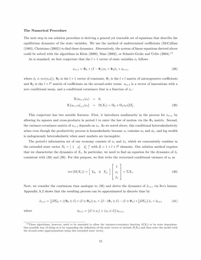
The Numerical Procedure

The next step in our solution procedure is deriving a general yet tractable set of equations that describe the

equilibrium dynamics of the state variables. We use the method of undetermined coeffi cients (McCallum

(1983), Christiano (2002)) to find these dynamics. Alternatively, the system of linear equations derived above

could be solved with the algorithms in Klein (2000), Sims (2002), or Schmitt-Grohe and Uribe (2004).12

As is standard, we first conjecture that the l × 1 vector of state variables xt follows

xt+1 = Φ0 + (I − Φ1)xt + Φ2xt + ut+1, (38)

where xt ≡ vec(xtx′t), Φ0 is the l× 1 vector of constants, Φ1 is the l× l matrix of autoregressive coeffi cientsand Φ2 is the l × l2 matrix of coeffi cients on the second-order terms. ut+1 is a vector of innovations with a

zero conditional mean, and a conditional covariance that is a function of xt :

E (ut+1|xt) = 0,

E(ut+1u

′t+1|xt

)= Ω(Xt) = Ω0 + Ω1xtx

′tΩ′1. (39)

This conjecture has two notable features: First, it introduces nonlinearity in the process for xt+1 by

allowing its squares and cross-products in period t to enter the law of motion via the Φ2 matrix. Second,

the variance-covariance matrix of xt+1 depends on xt. As we noted above, this conditional heteroskedasticity

arises even though the productivity process is homoskedastic because xt contains wt and wt, and log wealth

is endogenously heteroskedastic when asset markets are incomplete.

The period-t information set of our economy consists of xt and xt, which we conveniently combine in

the extended state vector Xt = [ 1 x′t x′t ]′ with L = 1 + l + l2 elements. Our solution method requires

that we characterize the dynamics of Xt. In particular, we need to find an equation for the dynamics of xt

consistent with (38) and (39). For this purpose, we first write the vectorized conditional variance of ut as

vec (Ω(Xt)) =[

Σ0 0 Σ1

]1

xt

xt

= ΣXt. (40)

Next, we consider the continuous time analogue to (38) and derive the dynamics of xt+1 via Ito’s lemma.

Appendix A.2 shows that the resulting process can be approximated in discrete time by

xt+1 = 12DΣ0 + ((Φ0 ⊗ I) + (I ⊗ Φ0))xt +

(I− (Φ1 ⊗ I)− (I ⊗ Φ1) + 1

2DΣ1

)xt + ut+1 (41)

where ut+1 = [(I ⊗ xt) + (xt ⊗ I)]ut+1,

12These algorithms, however, need to be amended to allow the variance-covariance function S(Xt) to be state dependent.One possible way of doing so is by expanding the definition of the state vector to include S(Xt) and then solve the model withthe second-order approximations using this extended state vector.

15

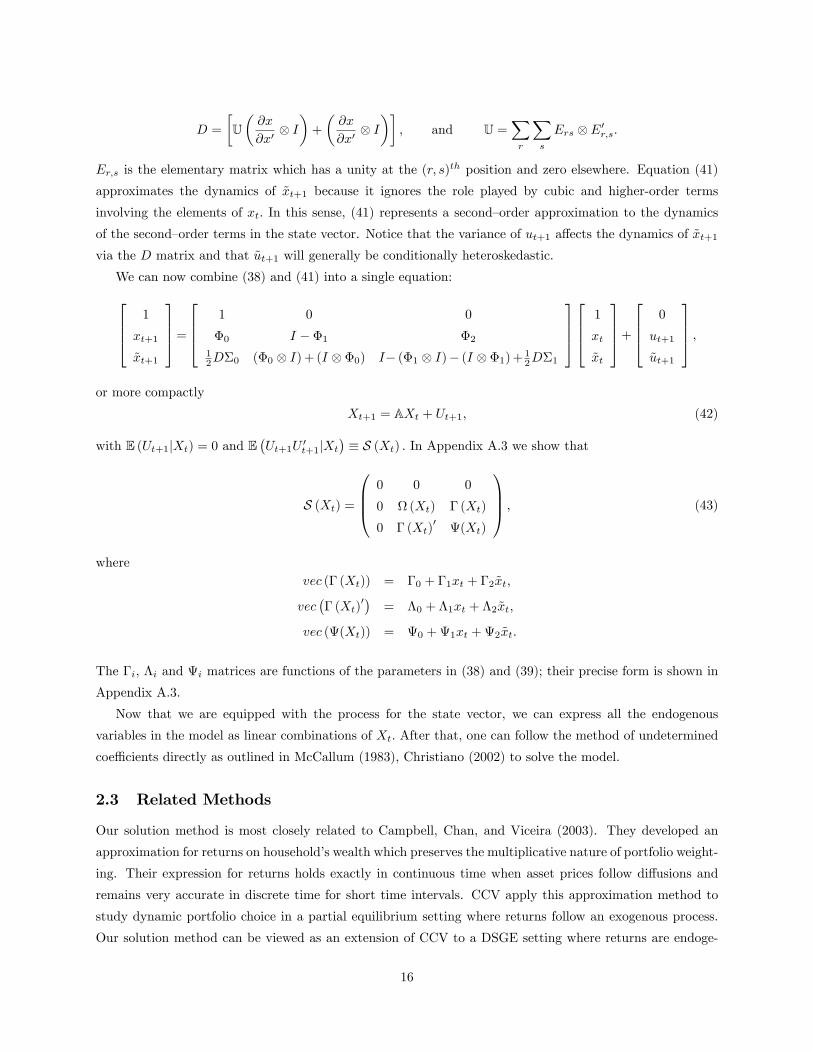
D =

[U(∂x

∂x′⊗ I)

+

(∂x

∂x′⊗ I)]

, and U =∑r

∑s

Ers ⊗ E′r,s.

Er,s is the elementary matrix which has a unity at the (r, s)th position and zero elsewhere. Equation (41)

approximates the dynamics of xt+1 because it ignores the role played by cubic and higher-order terms

involving the elements of xt. In this sense, (41) represents a second—order approximation to the dynamics

of the second—order terms in the state vector. Notice that the variance of ut+1 affects the dynamics of xt+1

via the D matrix and that ut+1 will generally be conditionally heteroskedastic.

We can now combine (38) and (41) into a single equation:1

xt+1

xt+1

=

1 0 0

Φ0 I − Φ1 Φ2

12DΣ0 (Φ0 ⊗ I) + (I ⊗ Φ0) I− (Φ1 ⊗ I)− (I ⊗ Φ1) + 1

2DΣ1

1

xt

xt

+

0

ut+1

ut+1

,or more compactly

Xt+1 = AXt + Ut+1, (42)

with E (Ut+1|Xt) = 0 and E(Ut+1U

′t+1|Xt

)≡ S (Xt) . In Appendix A.3 we show that

S (Xt) =

0 0 0

0 Ω (Xt) Γ (Xt)

0 Γ (Xt)′

Ψ(Xt)

, (43)

wherevec (Γ (Xt)) = Γ0 + Γ1xt + Γ2xt,

vec(Γ (Xt)

′)= Λ0 + Λ1xt + Λ2xt,

vec (Ψ(Xt)) = Ψ0 + Ψ1xt + Ψ2xt.

The Γi, Λi and Ψi matrices are functions of the parameters in (38) and (39); their precise form is shown in

Appendix A.3.

Now that we are equipped with the process for the state vector, we can express all the endogenous

variables in the model as linear combinations of Xt. After that, one can follow the method of undetermined

coeffi cients directly as outlined in McCallum (1983), Christiano (2002) to solve the model.

2.3 Related Methods

Our solution method is most closely related to Campbell, Chan, and Viceira (2003). They developed an

approximation for returns on household’s wealth which preserves the multiplicative nature of portfolio weight-

ing. Their expression for returns holds exactly in continuous time when asset prices follow diffusions and

remains very accurate in discrete time for short time intervals. CCV apply this approximation method to

study dynamic portfolio choice in a partial equilibrium setting where returns follow an exogenous process.

Our solution method can be viewed as an extension of CCV to a DSGE setting where returns are endoge-

16

nously determined.

Our approach also builds on the perturbation methods developed and applied in Judd and Guu (1993,

1997), Judd (1998), and further discussed in Collard and Juillard (2001), Jin and Judd (2002), Schmitt-

Grohe and Uribe (2004) among others. These methods extend solution techniques relying on linearizations

by allowing for second- and higher-order terms in the approximation of the policy functions. Applications of

the perturbation technique to models with portfolio choice have been developed in Devereux and Sutherland

(2008, 2007) and Tille and van Wincoop (2010). Both approaches are based on Taylor series approxima-

tions. Devereux and Sutherland (2008) use second-order approximations to the portfolio choice conditions

and first-order approximations to the other optimality conditions in order to calculate the steady state port-

folio allocations in a DSGE model. Our method also produces constant portfolio shares in the case where

equilibrium returns are i.i.d. because S (Xt) is a constant matrix.

To study time-variation in portfolio choice, Devereux and Sutherland (2007) and Tille and van Wincoop

(2010) use a method that incorporates third-order approximations of portfolio equations and second-order

approximations to the rest of the model’s equilibrium conditions. This approach delivers a first-order ap-

proximation for optimal portfolio holdings that vary with the state of the economy. By contrast, we are able

to derive second-order approximations to portfolio holdings from a set of second-order approximations to the

equilibrium conditions of the model and covariance function S (Xt). Approximating both first and second

moments of the state vector to the second-order allows us to implicitly characterize the portfolio optimality

conditions to the fourth order. This yields the second-order accurate dynamics of portfolio shares. If we

approximated S (Xt) to the first-order, we would obtain first-order variations in portfolio shares, as in Dev-

ereux and Sutherland (2007) and Tille and van Wincoop (2010). Thus, we are able to study the dynamics of

portfolio shares to a higher-order of accuracy while avoiding the numerical complexity of computing at least

third-order approximations. This aspect of our method will be important in models with larger number of

state variables and where agents choose between many assets. The model in Section 1 has 8 state variables

and five assets, but was solved without much computational diffi culty. We view this as an important prac-

tical advantage of our method that will make it particularly useful for solving international DSGE models.

By their very nature, even a minimally specified two-country DSGE model will have many state variables

and several assets. In Section 3.3 we also perform detailed accuracy comparisons of our method with that

in Devereux and Sutherland (2007).

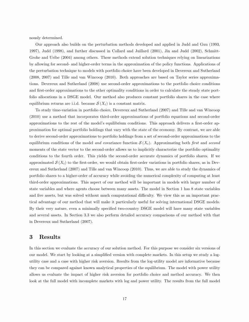
3 Results

In this section we evaluate the accuracy of our solution method. For this purpose we consider six versions of

our model. We start by looking at a simplified version with complete markets. In this setup we study a log-

utility case and a case with higher risk aversion. Results from the log-utility model are informative because

they can be compared against known analytical properties of the equilibrium. The model with power utility

allows us evaluate the impact of higher risk aversion for portfolio choice and method accuracy. We then

look at the full model with incomplete markets with log and power utility. The results from the full model

17

demonstrate the accuracy of our solution method in an application where no analytical characterization of

the equilibrium is available.

Our model simplifies considerably if we let (1 − φ)−1 → ∞, set σ = 1, require µt = 1 and µn = 0 in

both countries, and assume that the variance of nontraded productivity shocks equal zero. These restrictions

effectively eliminate the nontraded sectors in each country; the supply and demand for nontraded goods is

zero, and so too is the price of nontraded equity. The equilibrium properties of the other variables will be

identical to those in a world where households have log preferences defined over traded consumption and

allocate their portfolios between h and f traded equities and the risk-free bond. In particular, the equilibrium

will be characterized by complete risk-sharing if both h and f households start with the same initial level

of wealth. Furthermore, since markets are complete, the non-stationarity problem does not arise in this

simplified setup. So, we eliminate the endogenous discount factor in this version of our model by setting

β(Ctt , Cnt ) = β, ∀t, a constant.

Complete risk-sharing occurs in our simplified setting because all households have the same preferences

and investment opportunity sets. We can see why this is so by returning to the conditions determining the

households’portfolio choices. In particular, combining the log-approximated first-order conditions with the

budget constraint in (22) under the assumption of log preferences gives

αt = Θ−1t (Etert+1 + 1

2diag (Vt(ert+1)) and αt = Θ−1t (Etert+1 + 1

2diag(Vt(ert+1)), (44)

where α′t ≡ [ αht αft ], α′t ≡ [ αht αft ], er′t+1 ≡ [ rht+1 − rt rft+1 − rt ], and Θt ≡ Vt(ert+1). The key

point to note here is that all households face the same set of returns and have the same information. So the

right hand side of both expressions in (44) are identical in equilibrium. h and f households will therefore

find it optimal to hold the same portfolio shares. This has a number of implications if the initial distribution

of wealth is equal. First, households’wealth will be equalized across countries in all periods. Second, since

households with log utility consume a constant fraction of wealth, consumption will also be equalized. This

symmetry in consumption implies that mt+1 = mt+1, so risk sharing is complete. It also implies, together

with the market clearing conditions, that bond holdings are zero and wealth is equally split between h and

f equities (i.e., Aht = Aht = Aft = Aft = 1/2).We can use these equilibrium asset holdings as a benchmark for

judging the accuracy of our solution technique.

When σ 6= 1, we can again use the log-approximated Euler equations to show that the households’optimal

portfolio choices are given by

αt = 1σΘ−1

t (Etert+1 + 12diag (Vt(ert+1))−Θ−1

t CVt(λt+1, ert+1) and

αt = 1σΘ−1

t (Etert+1 + 12diag (Vt(ert+1))−Θ−1

t CVt(λt+1, ert+1).

These equations express the optimal portfolios as the sum of two components. The first term on the right-

hand-side is a familiar mean-variance component of asset demand. Except for the 1σ term, it coincides with

the solution under log-utility case. The second term is an intertemporal hedging demand. It depends on

the covariance between aggregate consumption-wealth ratio and excess returns. In the full 2-sector model

18

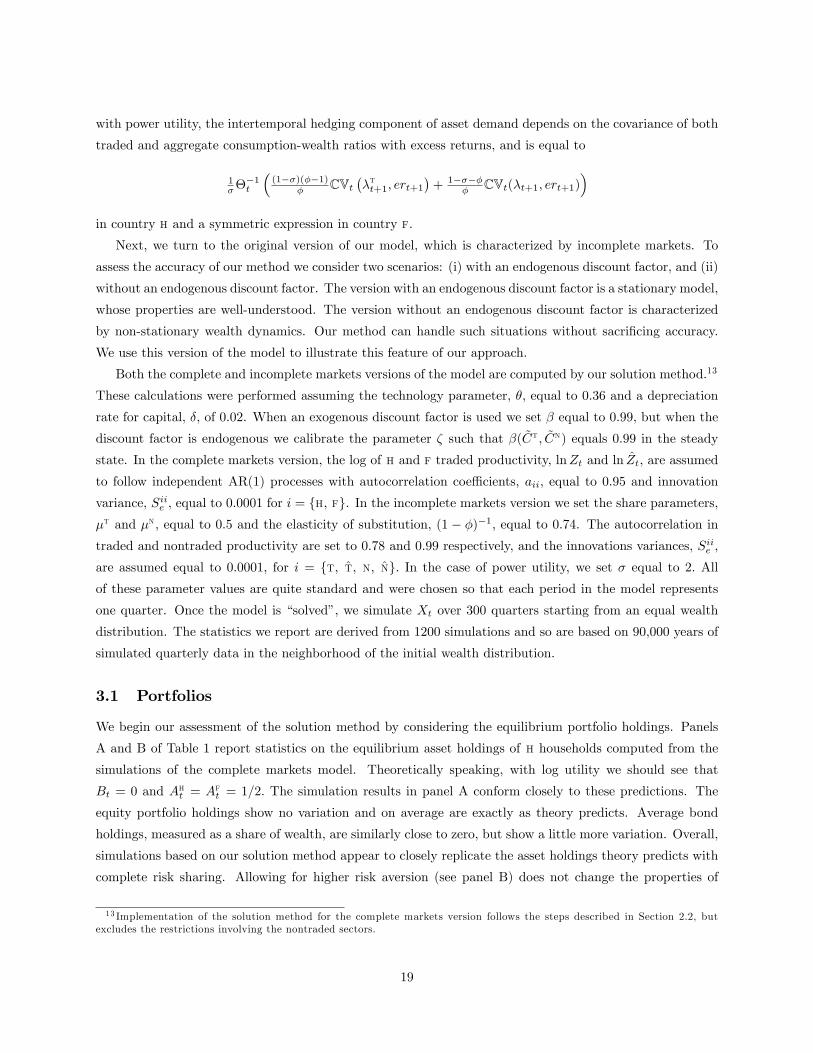
with power utility, the intertemporal hedging component of asset demand depends on the covariance of both

traded and aggregate consumption-wealth ratios with excess returns, and is equal to

1σΘ−1

t

((1−σ)(φ−1)

φ CVt(λtt+1, ert+1

)+ 1−σ−φ

φ CVt(λt+1, ert+1))

in country h and a symmetric expression in country f.

Next, we turn to the original version of our model, which is characterized by incomplete markets. To

assess the accuracy of our method we consider two scenarios: (i) with an endogenous discount factor, and (ii)

without an endogenous discount factor. The version with an endogenous discount factor is a stationary model,

whose properties are well-understood. The version without an endogenous discount factor is characterized

by non-stationary wealth dynamics. Our method can handle such situations without sacrificing accuracy.

We use this version of the model to illustrate this feature of our approach.

Both the complete and incomplete markets versions of the model are computed by our solution method.13

These calculations were performed assuming the technology parameter, θ, equal to 0.36 and a depreciation

rate for capital, δ, of 0.02. When an exogenous discount factor is used we set β equal to 0.99, but when the

discount factor is endogenous we calibrate the parameter ζ such that β(Ct, Cn) equals 0.99 in the steady

state. In the complete markets version, the log of h and f traded productivity, lnZt and ln Zt, are assumed

to follow independent AR(1) processes with autocorrelation coeffi cients, aii, equal to 0.95 and innovation

variance, Siie , equal to 0.0001 for i = h, f. In the incomplete markets version we set the share parameters,µt and µn, equal to 0.5 and the elasticity of substitution, (1 − φ)−1, equal to 0.74. The autocorrelation in

traded and nontraded productivity are set to 0.78 and 0.99 respectively, and the innovations variances, Siie ,

are assumed equal to 0.0001, for i = t, t, n, n. In the case of power utility, we set σ equal to 2. All

of these parameter values are quite standard and were chosen so that each period in the model represents

one quarter. Once the model is “solved”, we simulate Xt over 300 quarters starting from an equal wealth

distribution. The statistics we report are derived from 1200 simulations and so are based on 90,000 years of

simulated quarterly data in the neighborhood of the initial wealth distribution.

3.1 Portfolios

We begin our assessment of the solution method by considering the equilibrium portfolio holdings. Panels

A and B of Table 1 report statistics on the equilibrium asset holdings of h households computed from the

simulations of the complete markets model. Theoretically speaking, with log utility we should see that

Bt = 0 and Aht = Aft = 1/2. The simulation results in panel A conform closely to these predictions. The

equity portfolio holdings show no variation and on average are exactly as theory predicts. Average bond

holdings, measured as a share of wealth, are similarly close to zero, but show a little more variation. Overall,

simulations based on our solution method appear to closely replicate the asset holdings theory predicts with

complete risk sharing. Allowing for higher risk aversion (see panel B) does not change the properties of

13 Implementation of the solution method for the complete markets version follows the steps described in Section 2.2, butexcludes the restrictions involving the nontraded sectors.

19

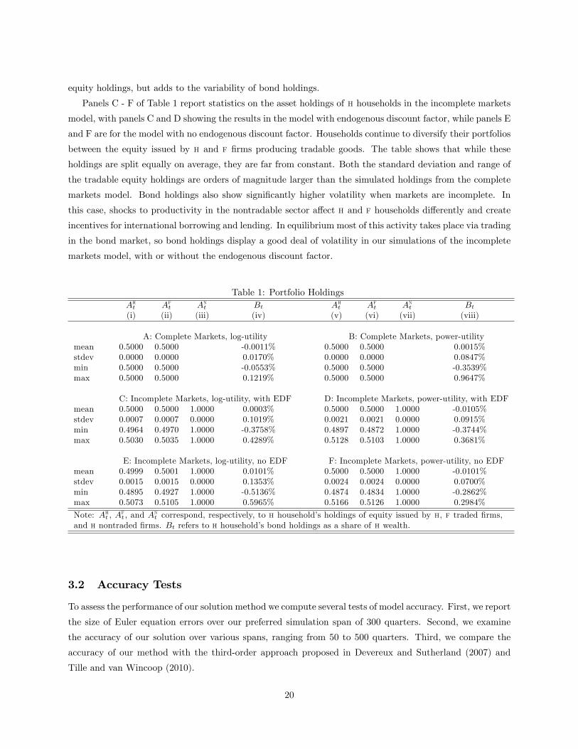
equity holdings, but adds to the variability of bond holdings.

Panels C - F of Table 1 report statistics on the asset holdings of h households in the incomplete markets

model, with panels C and D showing the results in the model with endogenous discount factor, while panels E

and F are for the model with no endogenous discount factor. Households continue to diversify their portfolios

between the equity issued by h and f firms producing tradable goods. The table shows that while these

holdings are split equally on average, they are far from constant. Both the standard deviation and range of

the tradable equity holdings are orders of magnitude larger than the simulated holdings from the complete

markets model. Bond holdings also show significantly higher volatility when markets are incomplete. In

this case, shocks to productivity in the nontradable sector affect h and f households differently and create

incentives for international borrowing and lending. In equilibrium most of this activity takes place via trading

in the bond market, so bond holdings display a good deal of volatility in our simulations of the incomplete

markets model, with or without the endogenous discount factor.

Table 1: Portfolio HoldingsAht Aft Ant Bt Aht Aft Ant Bt(i) (ii) (iii) (iv) (v) (vi) (vii) (viii)

A: Complete Markets, log-utility B: Complete Markets, power-utilitymean 0.5000 0.5000 -0.0011% 0.5000 0.5000 0.0015%stdev 0.0000 0.0000 0.0170% 0.0000 0.0000 0.0847%min 0.5000 0.5000 -0.0553% 0.5000 0.5000 -0.3539%max 0.5000 0.5000 0.1219% 0.5000 0.5000 0.9647%

C: Incomplete Markets, log-utility, with EDF D: Incomplete Markets, power-utility, with EDFmean 0.5000 0.5000 1.0000 0.0003% 0.5000 0.5000 1.0000 -0.0105%stdev 0.0007 0.0007 0.0000 0.1019% 0.0021 0.0021 0.0000 0.0915%min 0.4964 0.4970 1.0000 -0.3758% 0.4897 0.4872 1.0000 -0.3744%max 0.5030 0.5035 1.0000 0.4289% 0.5128 0.5103 1.0000 0.3681%

E: Incomplete Markets, log-utility, no EDF F: Incomplete Markets, power-utility, no EDFmean 0.4999 0.5001 1.0000 0.0101% 0.5000 0.5000 1.0000 -0.0101%stdev 0.0015 0.0015 0.0000 0.1353% 0.0024 0.0024 0.0000 0.0700%min 0.4895 0.4927 1.0000 -0.5136% 0.4874 0.4834 1.0000 -0.2862%max 0.5073 0.5105 1.0000 0.5965% 0.5166 0.5126 1.0000 0.2984%

Note: Aht , Aft , and A

nt correspond, respectively, to h household’s holdings of equity issued by h, f traded firms,

and h nontraded firms. Bt refers to h household’s bond holdings as a share of h wealth.

3.2 Accuracy Tests

To assess the performance of our solution method we compute several tests of model accuracy. First, we report

the size of Euler equation errors over our preferred simulation span of 300 quarters. Second, we examine

the accuracy of our solution over various spans, ranging from 50 to 500 quarters. Third, we compare the

accuracy of our method with the third-order approach proposed in Devereux and Sutherland (2007) and

Tille and van Wincoop (2010).

20

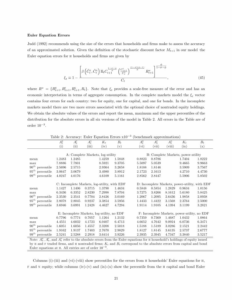
Euler Equation Errors

Judd (1992) recommends using the size of the errors that households and firms make to assess the accuracy

of an approximated solution. Given the definition of the stochastic discount factor Mt+1 in our model the

Euler equation errors for h households and firms are given by

ξt ≡ 1−

[β(Ctt , C

nt

)EtC

1−σ−φφ

t+1

(Ctt+1

Ctt

) (1−σ)(φ−1)φ

Rκt+1

] φ1−σ−φ

Ct, (45)

where Rκ = Rht+1, Rft+1, R

kt+1, Rt. Note that ξt provides a scale-free measure of the error and has an

economic interpretation in terms of aggregate consumption. In the complete markets model the ξt vector

contains four errors for each country: two for equity, one for capital, and one for bonds. In the incomplete

markets model there are two more errors associated with the optional choice of nontraded equity holdings.

We obtain the absolute values of the errors and report the mean, maximum and the upper percentiles of the

distribution for the absolute errors in all six versions of the model in Table 2. All errors in the Table are of

order 10−3.

Table 2: Accuracy: Euler Equation Errors x10−3 (benchmark approximations)Aht Aft Ant Kt Bt Aht Aft Ant Kt Bt(i) (ii) (iii) (iv) (v) (vi) (vii) (viii) (ix) (x)

A: Complete Markets, log-utility B: Complete Markets, power-utilitymean 1.2483 1.2485 1.4259 1.5848 0.8823 0.8786 1.7404 1.8222max 7.8886 7.7801 8.5921 9.3705 5.5097 5.0539 9.4665 9.966390th percentile 2.5696 2.5715 2.9364 3.2658 1.8188 1.8146 3.5909 3.756795th percentile 3.0647 3.0679 3.4980 3.8912 2.1723 2.1613 4.2710 4.473099th percentile 4.0247 4.0176 4.6109 5.1161 2.8562 2.8447 5.5906 5.8502

C: Incomplete Markets, log-utility, with EDF D: Incomplete Markets, power-utility, with EDFmean 1.1427 1.1406 0.3715 1.3790 1.4634 0.5848 0.5854 1.2829 0.9634 1.0156max 6.3436 6.3352 2.8230 7.2998 7.8704 3.7275 3.8266 8.1612 5.6180 5.842590th percentile 2.3530 2.3541 0.7704 2.8426 3.0169 1.2067 1.2095 2.6436 1.9858 2.093895th percentile 2.8078 2.8045 0.9237 3.3854 3.5956 1.4433 1.4422 3.1568 2.3764 2.500099th percentile 3.6946 3.6991 1.2428 4.4627 4.7294 1.9114 1.9105 4.1394 3.1199 3.2821

E: Incomplete Markets, log-utility, no EDF F: Incomplete Markets, power-utility, no EDFmean 0.7796 0.7774 0.7057 1.1264 1.2132 0.7359 0.7369 1.4687 1.0432 1.0864max 4.4551 4.6032 4.1723 6.0407 6.4713 4.6652 4.7642 9.0924 6.0736 6.347190th percentile 1.6051 1.6056 1.4557 2.3208 2.5018 1.5188 1.5189 3.0286 2.1521 2.244295th percentile 1.9162 1.9137 1.7403 2.7670 2.9829 1.8127 1.8145 3.6135 2.5737 2.677799th percentile 2.5241 2.5288 2.2918 3.6414 3.9226 2.3935 2.3945 4.7347 3.3840 3.5217

Note: Aht , Aft , and A

nt refer to the absolute errors from the Euler equations for h household’s holdings of equity issued

by h and f traded firms, and h nontraded firms; Kt and Bt correspond to the absolute errors from capital and bondEuler equations at h. All entries are of order 10−3.

Columns (i)-(iii) and (vi)-(viii) show percentiles for the errors from h households’Euler equations for h,

f and n equity; while columns (iv)-(v) and (ix)-(x) show the percentile from the h capital and bond Euler

21

equations, respectively. There are several features of the Euler equation distributions to note. First, the

Euler equation errors in all six models are small, with the largest error being less than 1 percent of aggregate

consumption. On average, the errors are about a tenth of 1 percent of consumption, with the higher numbers

obtained in the complete markets models. Second, the errors tend to be smaller in the models with power

utility. This is mainly due to lower elasticity of intertemporal substitution and smoother consumption

paths in these models. Finally, the presence of endogenous discount factor does not significantly affect

the distribution of Euler equation errors under incomplete markets, as the errors are comparable across

the versions with and without endogenous discount factor. Finally, we note that Euler equation errors

obtained using our method are comparable to those reported in the accuracy checks for standard growth

models without portfolio choice (e.g., Aruoba, Fernandez-Villaverde, and Rubio-Ramirez (2006) and Pichler

(2005)).14

The approximations we use to characterize the solution to non-stationary versions of the model are

only accurate in a neighborhood of the initial wealth distribution. If shocks to productivity push the wealth

distribution outside this neighborhood in a few periods with high probability, we will not be able to accurately

simulate long time series from the model’s equilibrium. This is not a concern for the models in this paper. To

illustrate this, we consider how the accuracy of the simulated equilibrium dynamics varies with the simulation

span. For this purpose we examine the distributions of Euler equation errors for different simulation spans.

To preserve space, we report the errors for the domestic equity holdings Euler equation in country h. The

results for all other Euler equation are analogous. Table 3 reports the results for all six models simulated

for various number of periods: 500, 400, 300 (our benchmark), 200, 100 and 50 quarters.

Euler equation errors in all six models are stable; including, importantly, the incomplete markets model

with no endogenous discount factor (panels E and F). Furthermore, while the errors occasionally rise with

the length of the simulation spans, the changes are moderate. Even at the horizon of 500 quarters, the

Euler equation errors are small, on the order of less than one tenth of 1 percent of aggregate consumption.

Overall, these results suggest that our method works well for both stationary and non-stationary versions of

the model.

Wealth Dynamics and Simulation Spans

As an additional check of the accuracy of our model we examine the distribution of errors in the bond market

clearing condition. Recall that the bond market clearing condition, Bt+Bt = 0, was not used in our method,

so the value of Bt+Bt implied by our solution provides a further accuracy check: If there is no approximation

error in the equations we use for the other market clearing conditions and budged constraints, Bt+Bt should

equal zero by Walras Law in our simulations of the model’s solution.15 We examine the accuracy of the

14 In the benchmark approximations described above we relied on the first-order approximations of the equations characterizingthe real side of the model and on the second-order approximations of the portfolio equations. We also solved all six versions ofthe model using second-order approximations of all equilibrium equations and computed the Euler equation errors from theseextended approximations. We find that there is very little difference between the distributions of these errors and those reportedin 2. The use of first- rather than second-order approximations to characterize the real side of the model does not appear toadversely affect the accuracy of our solution procedure. These results are available from the authors upon request.15We thank Anna Pavlova for suggesting this accuracy evaluation.

22

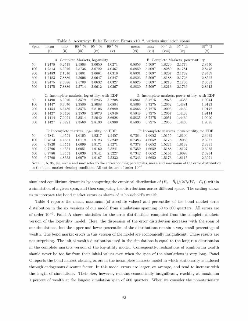
Table 3: Accuracy: Euler Equation Errors x10−3, various simulation spansSpan mean max 90th % 95th % 99th % mean max 90th % 95th % 99th %

(i) (ii) (iii) (iv) (v) (vi) (vii) (viii) (ix) (x)

A: Complete Markets, log-utility B: Complete Markets, power-utility50 1.2478 6.2519 2.5808 3.0650 4.0271 0.8856 5.5097 1.8220 2.1773 2.8440100 1.2513 6.3076 2.5736 3.0722 4.0467 0.8859 5.5097 1.8289 2.1781 2.8478200 1.2483 7.1610 2.5681 3.0661 4.0310 0.8831 5.5097 1.8207 2.1732 2.8469300 1.2483 7.8886 2.5696 3.0647 4.0247 0.8823 5.5097 1.8188 2.1723 2.8562400 1.2475 7.8886 2.5709 3.0632 4.0327 0.8828 5.5097 1.8213 2.1735 2.8583500 1.2475 7.8886 2.5714 3.0612 4.0267 0.8830 5.5097 1.8213 2.1736 2.8613

C: Incomplete markets, log-utility, with EDF D: Incomplete markets, power-utility, with EDF50 1.1490 6.3070 2.3579 2.8245 3.7208 0.5861 3.7275 1.2078 1.4386 1.9044100 1.1447 6.3070 2.3580 2.8088 3.6884 0.5866 3.7275 1.2062 1.4381 1.9123200 1.1454 6.3436 2.3575 2.8106 3.6989 0.5866 3.7275 1.2095 1.4439 1.9172300 1.1427 6.3436 2.3530 2.8078 3.6946 0.5848 3.7275 1.2067 1.4433 1.9114400 1.1414 7.0921 2.3514 2.8042 3.6928 0.5835 3.7275 1.2051 1.4430 1.9090500 1.1427 7.0921 2.3569 2.8133 3.6980 0.5833 3.7275 1.2055 1.4430 1.9095

E: Incomplete markets, log-utility, no EDF F: Incomplete markets, power-utility, no EDF50 0.7841 4.4551 1.6105 1.9217 2.5457 0.7384 4.6652 1.5155 1.8100 2.3935100 0.7813 4.4551 1.6119 1.9123 2.5232 0.7383 4.6652 1.5176 1.8063 2.3937200 0.7820 4.4551 1.6099 1.9171 2.5271 0.7378 4.6652 1.5224 1.8132 2.3991300 0.7796 4.4551 1.6051 1.9162 2.5241 0.7359 4.6652 1.5188 1.8127 2.3935400 0.7786 4.8553 1.6039 1.9141 2.5227 0.7342 4.6652 1.5164 1.8098 2.3934500 0.7790 4.8553 1.6079 1.9167 2.5232 0.7343 4.6652 1.5173 1.8115 2.3921

Note: 1, 5, 95, 99, mean and max refer to the corresponding percentiles, mean and maximum of the error distributionin the bond market clearing condition. All entries are of order 10−3.

simulated equilibrium dynamics by computing the empirical distribution of (Bt+ Bt)/(2Rt(Wt−Ct)) withina simulation of a given span, and then comparing the distributions across different spans. The scaling allows

us to interpret the bond market errors as shares of h household’s wealth.

Table 4 reports the mean, maximum (of absolute values) and percentiles of the bond market error

distribution in the six versions of our model from simulations spanning 50 to 500 quarters. All errors are

of order 10−3. Panel A shows statistics for the error distributions computed from the complete markets

version of the log-utility model. Here, the dispersion of the error distribution increases with the span of

our simulations, but the upper and lower percentiles of the distributions remain a very small percentage of

wealth. The bond market errors in this version of the model are economically insignificant. These results are

not surprising. The initial wealth distribution used in the simulations is equal to the long run distribution

in the complete markets version of the log-utility model. Consequently, realizations of equilibrium wealth

should never be too far from their initial values even when the span of the simulations is very long. Panel

C reports the bond market clearing errors in the incomplete markets model in which stationarity is induced

through endogenous discount factor. In this model errors are larger, on average, and tend to increase with

the length of simulations. Their size, however, remains economically insignificant, reaching at maximum

1 percent of wealth at the longest simulation span of 500 quarters. When we consider the non-stationary

23

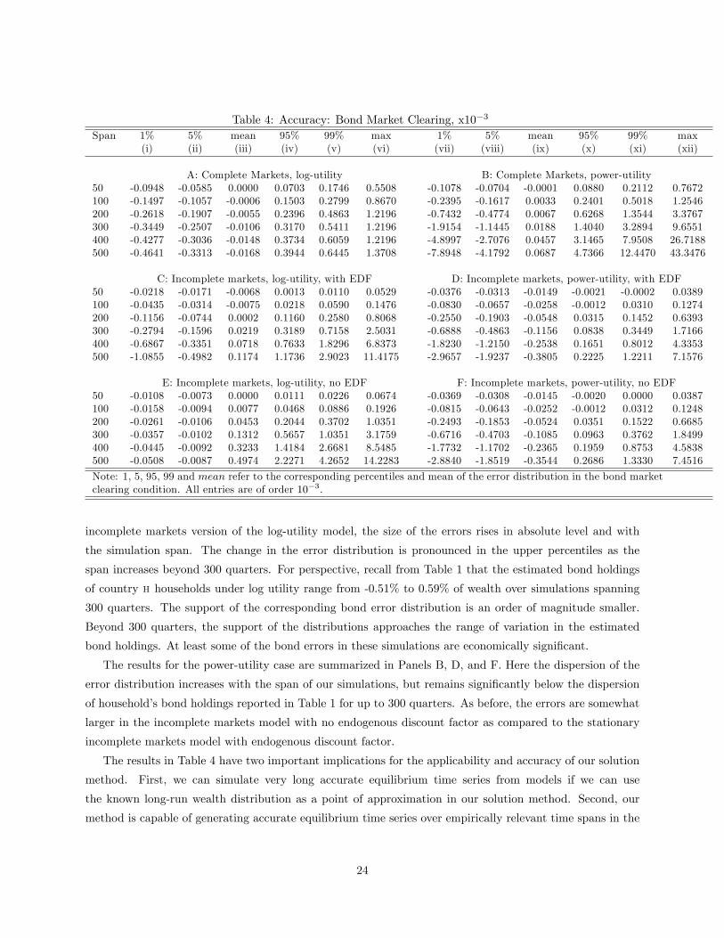
Table 4: Accuracy: Bond Market Clearing, x10−3

Span 1% 5% mean 95% 99% max 1% 5% mean 95% 99% max(i) (ii) (iii) (iv) (v) (vi) (vii) (viii) (ix) (x) (xi) (xii)

A: Complete Markets, log-utility B: Complete Markets, power-utility50 -0.0948 -0.0585 0.0000 0.0703 0.1746 0.5508 -0.1078 -0.0704 -0.0001 0.0880 0.2112 0.7672100 -0.1497 -0.1057 -0.0006 0.1503 0.2799 0.8670 -0.2395 -0.1617 0.0033 0.2401 0.5018 1.2546200 -0.2618 -0.1907 -0.0055 0.2396 0.4863 1.2196 -0.7432 -0.4774 0.0067 0.6268 1.3544 3.3767300 -0.3449 -0.2507 -0.0106 0.3170 0.5411 1.2196 -1.9154 -1.1445 0.0188 1.4040 3.2894 9.6551400 -0.4277 -0.3036 -0.0148 0.3734 0.6059 1.2196 -4.8997 -2.7076 0.0457 3.1465 7.9508 26.7188500 -0.4641 -0.3313 -0.0168 0.3944 0.6445 1.3708 -7.8948 -4.1792 0.0687 4.7366 12.4470 43.3476

C: Incomplete markets, log-utility, with EDF D: Incomplete markets, power-utility, with EDF50 -0.0218 -0.0171 -0.0068 0.0013 0.0110 0.0529 -0.0376 -0.0313 -0.0149 -0.0021 -0.0002 0.0389100 -0.0435 -0.0314 -0.0075 0.0218 0.0590 0.1476 -0.0830 -0.0657 -0.0258 -0.0012 0.0310 0.1274200 -0.1156 -0.0744 0.0002 0.1160 0.2580 0.8068 -0.2550 -0.1903 -0.0548 0.0315 0.1452 0.6393300 -0.2794 -0.1596 0.0219 0.3189 0.7158 2.5031 -0.6888 -0.4863 -0.1156 0.0838 0.3449 1.7166400 -0.6867 -0.3351 0.0718 0.7633 1.8296 6.8373 -1.8230 -1.2150 -0.2538 0.1651 0.8012 4.3353500 -1.0855 -0.4982 0.1174 1.1736 2.9023 11.4175 -2.9657 -1.9237 -0.3805 0.2225 1.2211 7.1576

E: Incomplete markets, log-utility, no EDF F: Incomplete markets, power-utility, no EDF50 -0.0108 -0.0073 0.0000 0.0111 0.0226 0.0674 -0.0369 -0.0308 -0.0145 -0.0020 0.0000 0.0387100 -0.0158 -0.0094 0.0077 0.0468 0.0886 0.1926 -0.0815 -0.0643 -0.0252 -0.0012 0.0312 0.1248200 -0.0261 -0.0106 0.0453 0.2044 0.3702 1.0351 -0.2493 -0.1853 -0.0524 0.0351 0.1522 0.6685300 -0.0357 -0.0102 0.1312 0.5657 1.0351 3.1759 -0.6716 -0.4703 -0.1085 0.0963 0.3762 1.8499400 -0.0445 -0.0092 0.3233 1.4184 2.6681 8.5485 -1.7732 -1.1702 -0.2365 0.1959 0.8753 4.5838500 -0.0508 -0.0087 0.4974 2.2271 4.2652 14.2283 -2.8840 -1.8519 -0.3544 0.2686 1.3330 7.4516

Note: 1, 5, 95, 99 and mean refer to the corresponding percentiles and mean of the error distribution in the bond marketclearing condition. All entries are of order 10−3.

incomplete markets version of the log-utility model, the size of the errors rises in absolute level and with

the simulation span. The change in the error distribution is pronounced in the upper percentiles as the

span increases beyond 300 quarters. For perspective, recall from Table 1 that the estimated bond holdings

of country h households under log utility range from -0.51% to 0.59% of wealth over simulations spanning

300 quarters. The support of the corresponding bond error distribution is an order of magnitude smaller.

Beyond 300 quarters, the support of the distributions approaches the range of variation in the estimated

bond holdings. At least some of the bond errors in these simulations are economically significant.

The results for the power-utility case are summarized in Panels B, D, and F. Here the dispersion of the

error distribution increases with the span of our simulations, but remains significantly below the dispersion

of household’s bond holdings reported in Table 1 for up to 300 quarters. As before, the errors are somewhat

larger in the incomplete markets model with no endogenous discount factor as compared to the stationary

incomplete markets model with endogenous discount factor.

The results in Table 4 have two important implications for the applicability and accuracy of our solution

method. First, we can simulate very long accurate equilibrium time series from models if we can use

the known long-run wealth distribution as a point of approximation in our solution method. Second, our

method is capable of generating accurate equilibrium time series over empirically relevant time spans in the

24

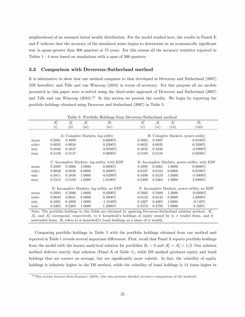
neighborhood of an assumed initial wealth distribution. For the model studied here, the results in Panels E

and F indicate that the accuracy of the simulated series begins to deteriorate in an economically significant

way in spans greater than 300 quarters or 75 years. For this reason all the accuracy statistics reported in

Tables 1 - 4 were based on simulations with a span of 300 quarters.

3.3 Comparison with Devereux-Sutherland method

It is informative to show how our method compares to that developed in Devereux and Sutherland (2007)

(DS hereafter) and Tille and van Wincoop (2010) in terms of accuracy. For this purpose all six models

presented in this paper were re-solved using the third-order approach of Devereux and Sutherland (2007)

and Tille and van Wincoop (2010).16 In this section we present the results. We begin by reporting the

portfolio holdings obtained using Devereux and Sutherland (2007) in Table 5.

Table 5: Portfolio Holdings from Devereux-Sutherland methodAht Aft Ant Bt Aht Aft Ant Bt(i) (ii) (iii) (iv) (v) (vi) (vii) (viii)

A: Complete Markets, log-utility B: Complete Markets, power-utilitymean 0.5001 0.4999 0.0000% 0.5002 0.4997 0.0100%stdev 0.0035 0.0034 0.2300% 0.0035 0.0035 0.2300%min 0.4848 0.4847 -0.9500% 0.4855 0.4838 -0.8900%max 0.5138 0.5147 0.9600% 0.5169 0.5150 0.9500%

C: Incomplete Markets, log-utility, with EDF D: Incomplete Markets, power-utility, with EDFmean 0.5000 0.5000 1.0000 0.0000% 0.4998 0.5001 1.0000 0.0000%stdev 0.0039 0.0039 0.0000 0.2000% 0.0107 0.0104 0.0000 0.9100%min 0.4811 0.4838 1.0000 -0.8200% 0.4490 0.4523 1.0000 -4.5000%max 0.5213 0.5193 1.0000 1.0100% 0.5460 0.5464 1.0000 3.8900%

E: Incomplete Markets, log-utility, no EDF F: Incomplete Markets, power-utility, no EDFmean 0.5003 0.5000 1.0000 0.0200% 0.5003 0.5000 1.0000 -0.0200%stdev 0.0040 0.0041 0.0000 0.2800% 0.0132 0.0132 0.0000 1.6800%min 0.4801 0.4809 1.0000 -1.2100% 0.4307 0.4365 1.0000 -9.140%max 0.5205 0.5205 1.0000 1.2000% 0.5573 0.5793 1.0000 8.100%

Note: The portfolio holdings in this Table are obtained by applying Devereux-Sutherland solution method. Aht ,Aft , and A

nt correspond, respectively, to h household’s holdings of equity issued by h, f traded firms, and h

nontraded firms. Bt refers to h household’s bond holdings as a share of h wealth.

Comparing portfolio holdings in Table 5 with the portfolio holdings obtained from our method and

reported in Table 1 reveals several important differences. First, recall that Panel A reports portfolio holdings

from the model with the known analytical solution for portfolios Bt = 0 and Aht = Aft = 1/2. Our solution

method delivers exactly that solution (Panel A of Table 1), while DS method produces equity and bond

holdings that are correct on average, but are significantly more volatile. In fact, the volatility of equity

holdings is infinitely higher in the DS method, while the volatility of bond holdings is 14 times higher in

16This section borrows from Kazimov (2010), who also presents detailed accuracy comparisons of the methods.

25

their method relative to our approach. Second, the higher volatility of portfolio holdings in the DS method

extends to all other models considered in this paper and is particularly pronounced for bond holdings.

Next, we compare the accuracy of our method relative to DS using Euler equation errors. For brevity

we report a summary measure of the errors which is computed from the portfolio Euler equation. Interested

reader is referred to Kazimov (2010) who reports the Euler equation errors from the individual Euler equations

and for all six models presented in this paper after solving them with the DS method.

Table 6 presents the mean, max, and the upper percentiles of the distribution of the absolute errors from

the portfolio Euler equation obtained from equation (45) with Rκ = Rwt+1.

Table 6: Portfolio Euler equation errors x10−3

Complete marketsA: Log utility B: Power utilityEH DS EH DS

mean 0.0010 2.1256 0.6239 2.1306max 0.0010 13.6812 3.3746 11.801990th percentile 0.0010 4.3925 1.2864 4.392295th percentile 0.0010 5.2219 1.5309 5.244799th percentile 0.0010 6.8736 2.0054 6.9020

Incomplete markets, with EDFC: Log utility D: Power utilityEH DS EH DS

mean 0.4101 1.6629 0.9121 1.2042max 2.3609 9.5096 5.9565 6.797490th percentile 0.8490 3.4324 1.8811 2.475895th percentile 1.0182 4.0818 2.2493 2.948199th percentile 1.3591 5.3646 2.9557 3.8613

Incomplete markets, no EDFE: Log utility F: Power utilityEH DS EH DS

mean 0.0349 1.6383 1.0898 1.3176max 0.6013 9.3046 6.8903 7.180490th percentile 0.0881 3.3695 2.2445 2.717595th percentile 0.1220 4.0138 2.6816 3.221399th percentile 0.2070 5.3348 3.5172 4.2534Note: This Table reports the errors from portfolio Euler equationin our method (denoted by EH) and in the Devereux-Sutherlandmethod (denoted by DS). All errors are of the order 10−3.

Notice that the portfolio Euler equation errors obtained using our solution method are comparable with

the errors in the individual Euler equations, and on many occasions are even smaller. But more importantly,

portfolio Euler equation errors obtained using our method are singificantly smaller than the portfolio Euler

equation errors obtained using DS solution method. This conclusion applies to all six models considered in

the paper. These comparisons highlight the accuracy of our method relative to the existing approaches.

26

4 Conclusion

We have presented a numerical method for solving general equilibrium models with many financial assets,

heterogeneous agents and incomplete markets. Our method builds on the log-approximations of Campbell,

Chan, and Viceira (2003) and the second-order perturbation technique developed by Judd (1998) and others.

To illustrate its use, we applied our solution method to complete and incomplete markets versions of a

two-country general equilibrium model with production, and to the versions of the model with log- and

power-utility. The numerical solution to the complete markets version closely conforms to the predictions of

theory and is highly accurate based on a number of standard tests. This gives us confidence in the accuracy

of our technique. The power of our method is illustrated by solving the incomplete markets version of the

model. The array of assets in this model is insuffi cient to permit complete risk-sharing among households, so

the equilibrium allocations cannot be found by standard analytical techniques. Our accuracy tests show that

simulations of our solution to this version of the model are very accurate over spans of 75 years of quarterly

data. Our solution method can be applied to more richly specified models than the one examined here. For

example, the method can be applied to solve models with more complex preferences, capital adjustment

costs, or portfolio constraints. As a result, we believe that our method will be useful in the future analysis

of many models in international macroeconomics and finance.

27

References

Aruoba, S. B., J. Fernandez-Villaverde, and J. F. Rubio-Ramirez (2006): “Comparing solution

methods for dynamic equilibrium economies,”Journal of Economic Dynamics and Control, 30(12), 2477—

2508.

Barberis, N. (2000): “Investing for the Long Run when Returns Are Predictable,” Journal of Finance,

55(1), 225—264.

Baxter, M., and M. J. Crucini (1995): “Business Cycles and the Asset Structure of Foreign Trade,”

International Economic Review, 36(4), 821—854.

Baxter, M., U. J. Jermann, and R. G. King (1998): “Nontraded Goods, Nontraded Factors, and

International Non-diversification,”Journal of International Economics, 44(2), 211—229.

Boileau, M., and M. Normandin (2008): “Closing international real business cycle models with restricted

financial markets,”Journal of International Money and Finance, 27(5), 733—756.

Brandt, M. W., A. Goyal, P. Santa-Clara, and J. R. Stroud (2005): “A Simulation Approach

to Dynamic Portfolio Choice with an Application to Learning About Return Predictability,”Review of

Financial Studies, 18(3), 831—873.

Brandt, M. W., and P. Santa-Clara (2004): “Dynamic Portfolio Selection by Augmenting the Asset

Space,”NBER Working Papers 10372, National Bureau of Economic Research, Inc.

Brennan, M., E. Schwartz, and R. Lagnado (1997): “Strategic asset allocation,”Journal of Economic

Dynamics and Control, 21(8-9), 1377—1403.

Campbell, J. Y., Y. L. Chan, and L. M. Viceira (2003): “A Multivariate Model of Strategic Asset

Allocation,”Journal of Financial Economics, 67(1), 41—80.

Campbell, J. Y., and R. J. Shiller (1988): “The Dividend-Price Ratio and Expectations of Future

Dividends and Discount Factors,”Review of Financial Studies, 1(3), 195—228.

Campbell, J. Y., and L. M. Viceira (2002): Strategic Asset Allocation. Oxford University Press.

Christiano, L. J. (2002): “Solving Dynamic Equilibrium Models by a Method of Undetermined Coeffi -

cients,”Computational Economics, 20(1-2), 21—55.

Collard, F., and M. Juillard (2001): “Accuracy of stochastic perturbation methods: The case of asset

pricing models,”Journal of Economic Dynamics and Control, 25(6-7), 979—999.

Correia, I., J. C. Neves, and S. Rebelo (1995): “Business cycles in a small open economy,”European

Economic Review, 39(6), 1089—1113.

Corsetti, G., L. Dedola, and S. Leduc (2008): “International Risk Sharing and the Transmission of

Productivity Shocks,”Review of Economic Studies, 75(2), 443—473.

28

Denis, C., and H. Huizinga (2004): “Are Foreign Ownership and Good Institutions Substitutes? The

Case of Non-Traded Equity,”CEPR Discussion Papers 4339, C.E.P.R. Discussion Papers.

Devereux, M. B., and A. Sutherland (2007): “Country Portfolio Dynamics,”CEPR Discussion Papers

6208.

(2008): “Country Portfolios in Open Economy Macro Models,” NBER Working Paper 14372,

National Bureau of Economic Research, Inc.

Engel, C., and A. Matsumoto (2009): “The International Diversification Puzzle When Goods Prices Are

Sticky: It’s Really about Exchange-Rate Hedging, Not Equity Portfolios,”American Economic Journal:

Macroeconomics, 1(2), 155—88.

Evans, M., and V. V. Hnatkovska (2005): “International Capital Flows, Returns and World Financial

Integration,”Georgetown University Working Paper and NBER Working Paper 11701.

Ghironi, F., J. Lee, and A. Rebucci (2009): “The Valuation Channel of External Adjustment,” IMF

Working Papers 09/275, International Monetary Fund.

Gourinchas, P.-O. (2006): “The Research Agenda: Pierre-Olivier Gourinchas on Global Imbalances and

Financial Factors,”EconomicDynamics Newsletter, 7(2).

Heathcote, J., and F. Perri (2004): “The International Diversification Puzzle is not as Bad as You

Think,”Working paper, Georgetown University.

Hnatkovska, V. (2010): “Home bias and high turnover: Dynamic portfolio choice with incomplete mar-

kets,”Journal of International Economics, 80(1), 113—128.

Jin, H.-H., and K. L. Judd (2002): “Perturbation Methods for General Dynamic Stochastic Models,”

Working papers, Stanford University.

Judd, K. L. (1992): “Projection Methods for Solving Aggregate Growth Models,” Journal of Economic

Theory, 58(2), 410—452.

(1998): Numerical Methods in Economics, vol. 1 of MIT Press Books. The MIT Press.

Judd, K. L., and S.-M. Guu (1993): “Perturbation Solution Methods for Economic Growth Models,” in

Economic and Financial Modeling with Mathematica, ed. by H. Varian. Springer-Verlag: New York.

(1997): “Asymptotic methods for aggregate growth models,”Journal of Economic Dynamics and

Control, 21(6), 1025—1042.

Kang, J.-K., and R. M. Stulz (1997): “Why is there a home bias? An analysis of foreign portfolio equity

ownership in Japan,”Journal of Financial Economics, 46(1), 3—28.

Kazimov, K. (2010): “Comparing Methods for Solving GE Models with Portfolio Choice,” manuscript,

Georgetown University.

29

Klein, P. (2000): “Using the generalized Schur form to solve a multivariate linear rational expectations

model,”Journal of Economic Dynamics and Control, 24(10), 1405—1423.

Kogan, L., and R. Uppal (2002): “Risk Aversion and Optimal Portfolio Policies in Partial and General

Equilibrium Economies,”Discussion Paper No. 3306, CEPR.

Kollmann, R. (1996): “Incomplete Asset Markets and the Cross-Country Consumption Correlation Puz-

zle,”Journal of Economic Dynamics and Control, 20(5), 945—961.

(2006): “International Portfolio Equilibrium and the Current Account: A Dynamic General Equi-

librium Perspective,”Mimeo, Free University of Brussels.

McCallum, B. T. (1983): “On non-uniqueness in rational expectations models : An attempt at perspec-

tive,”Journal of Monetary Economics, 11(2), 139—168.

Obstfeld, M. (2004): “External adjustment,”Review of World Economics (Weltwirtschaftliches Archiv),

140(4), 541—568.

Obstfeld, M., and K. Rogoff (1995): “Exchange Rate Dynamics Redux,”Journal of Political Economy,

103(3), 624—60.

Obstfeld, M., and K. Rogoff (1996): Foundations of International Macroeconomics. MIT Press Cam-

bridge, MA.

Pesenti, P., and E. van Wincoop (2002): “Can Nontradables Generate Substantial Home Bias?,”Journal

of Money, Credit and Banking, 34(1), 25—50.

Pichler, P. (2005): “Evaluating Approximate Equilibria of Dynamic Economic Models,”Vienna Economics

Papers 0510, University of Vienna, Department of Economics.

Schmitt-Grohe, S., and M. Uribe (2003): “Closing small open economy models,” Journal of Interna-

tional Economics, 61(1), 163—185.

(2004): “Solving Dynamic General Equilibrium Models Using a Second-Order Approximation to

the Policy Function,”Journal of Economic Dynamics and Control, 28(4), 755—775.

Serrat, A. (2001): “A Dynamic Equilibrium Model of International Portfolio Holdings,” Econometrica,

69(6), 1467—1489.

Sims, C. A. (2002): “Solving Linear Rational Expectations Models,”Computational Economics, 20(1-2),

1—20.

Tille, C., and E. van Wincoop (2010): “International Capital Flows,” Journal of International Eco-

nomics, 80(2), 157—175.

Uppal, R. (1993): “A General Equilibrium Model of International Portfolio Choice,”Journal of Finance,

48(2), 529—53.

30

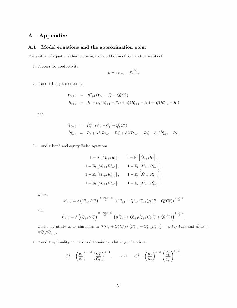
A Appendix:

A.1 Model equations and the approximation point

The system of equations characterizing the equilibrium of our model consists of

1. Process for productivity

zt = azt−1 + S1/2

e et

2. h and f budget constraints

Wt+1 = Rwt+1 (Wt − Ctt −QntCnt )

Rwt+1 = Rt + αht (Rht+1 −Rt) + αft (R

ft+1 −Rt) + αnt (R

nt+1 −Rt)

and

Wt+1 = Rwt+1(Wt − Ctt − Qnt Cnt )

Rwt+1 = Rt + αht (Rht+1 −Rt) + αft (R

ft+1 −Rt) + αnt (R

nt+1 −Rt).

3. h and f bond and equity Euler equations

1 = Et [Mt+1Rt] , 1 = Et[Mt+1Rt

],

1 = Et[Mt+1R

ht+1

], 1 = Et

[Mt+1R

ht+1

],

1 = Et[Mt+1R

ft+1

], 1 = Et

[Mt+1R

ft+1

],

1 = Et[Mt+1R

nt+1

], 1 = Et

[Mt+1R

nt+1

],

where

Mt+1 = β(Ctt+1/C

tt

) (1−σ)(φ−1)φ

((Ctt+1 +Qnt+1C

nt+1)/(Ctt +QntC

nt )) 1−σ−φ

φ

and

Mt+1 = β(Ctt+1/C

tt

) (1−σ)(φ−1)φ

((Ctt+1 + Qnt+1C

nt+1)/(Ctt + Qnt C

nt )) 1−σ−φ

φ

.

Under log-utility Mt+1 simplifies to β (Ctt +QntCnt ) /

(Ctt+1 +Qnt+1C

nt+1

)= βWt/Wt+1 and Mt+1 =

βWt/Wt+1.

4. h and f optimality conditions determining relative goods prices

Qnt =

(µnµt

)1−φ(CntCtt

)φ−1

, and Qnt =

(µnµt

)1−φ(Cnt

Ctt

)φ−1

.

A1

5. Capital Euler equation at h and f

1 = Et[Mt+1R

kt+1

], with Rkt+1 ≡ θZtt+1 (Kt+1)

θ−1+ (1− δ)

1 = Et[Mt+1R

kt+1

], with Rkt+1 ≡ θZtt+1(Kt+1)θ−1 + (1− δ)

6. From the portfolio Euler equation in each country, 1 = Et[Mt+1Rwt+1] and 1 = Et[Mt+1R

wt+1], after

substituting for Mt+1 and Mt+1 we get the expressions for consumption-wealth ratios

Λt(1−σ)(φ−1)

φ

t Λ1−σ−φφ

t (1− Λt)σ

= βEt[Λt

(1−σ)(φ−1)φ

t+1 Λ1−σ−φφ

t+1

(Rwt+1

)1−σ]Λt

(1−σ)(φ−1)φ

t Λ1−σ−φφ

t

(1− Λt

)σ= βEt

[Λt

(1−σ)(φ−1)φ

t+1 Λ1−σ−φφ

t+1

(Rwt+1

)1−σ].

7. Market clearing conditions

(a) traded goods

Ctt + Ctt = Dtt + Dt

t

(b) nontraded goods

Cnt = Y nt = Dnt and Cnt = Y nt = Dn

t .

(c) bond

0 = Bt + Bt.

(d) traded equity

1 = Aht + Aht and 1 = Aft + Aft ,

which can equivalently be written as

P tt = αht (Wt − Ct) + αht

(Wt − Ct

)P tt = αft (Wt − Ct) + αft

(Wt − Ct

)(e) nontraded equity

1 = Ant 1 = Ant ,

which is equivalent to

αnt = QntPnt / (Wt − Ct) αnt = Qnt P

nt /(Wt − Ct

).

The approximation point is given by the steady state levels of the following variables: R = Rk = Rk =

Rh = Rf = Rn = Rn = Rw = Rw = 1β . K = K = (βθ)

1/(1−θ)(1− β + βδ)

1/(θ−1), Dt = Dt = Kθ − δK,

P t = P t = βDt/(1 − β). Dn = Dn = η, so that Cn = Cn = η and P n = P n = βη/(1 − β). As we

A2

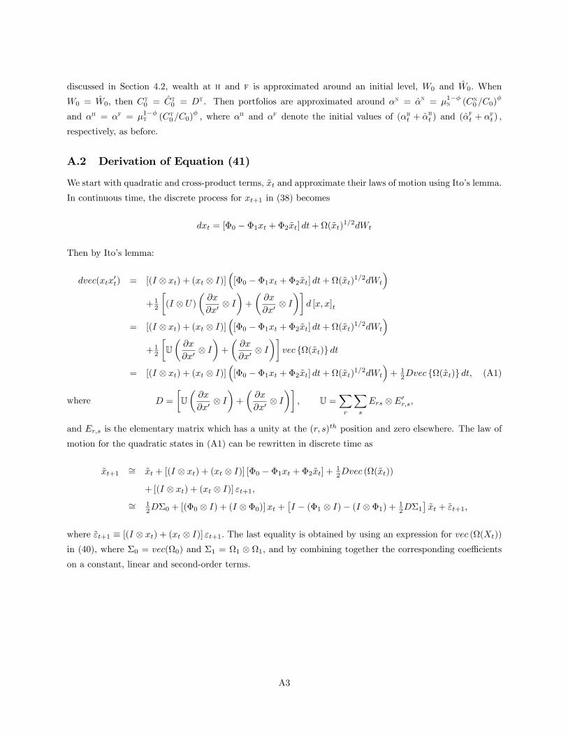
discussed in Section 4.2, wealth at h and f is approximated around an initial level, W0 and W0. When

W0 = W0, then Ct0 = Ct0 = Dt. Then portfolios are approximated around αn = αn = µ1−φn (Cn0 /C0)

φ

and αh = αf = µ1−φt (Ct0/C0)

φ, where αh and αf denote the initial values of (αht + αht ) and (αft + αft ) ,

respectively, as before.

A.2 Derivation of Equation (41)

We start with quadratic and cross-product terms, xt and approximate their laws of motion using Ito’s lemma.

In continuous time, the discrete process for xt+1 in (38) becomes

dxt = [Φ0 − Φ1xt + Φ2xt] dt+ Ω(xt)1/2dWt

Then by Ito’s lemma:

dvec(xtx′t) = [(I ⊗ xt) + (xt ⊗ I)]

([Φ0 − Φ1xt + Φ2xt] dt+ Ω(xt)

1/2dWt

)+ 1

2

[(I ⊗ U)

(∂x

∂x′⊗ I)

+

(∂x

∂x′⊗ I)]

d [x, x]t

= [(I ⊗ xt) + (xt ⊗ I)](

[Φ0 − Φ1xt + Φ2xt] dt+ Ω(xt)1/2dWt

)+ 1

2

[U(∂x

∂x′⊗ I)

+

(∂x

∂x′⊗ I)]

vec Ω(xt) dt

= [(I ⊗ xt) + (xt ⊗ I)](

[Φ0 − Φ1xt + Φ2xt] dt+ Ω(xt)1/2dWt

)+ 1

2Dvec Ω(xt) dt, (A1)

where D =

[U(∂x

∂x′⊗ I)

+

(∂x

∂x′⊗ I)]

, U =∑r

∑s

Ers ⊗ E′r,s,

and Er,s is the elementary matrix which has a unity at the (r, s)th position and zero elsewhere. The law of

motion for the quadratic states in (A1) can be rewritten in discrete time as

xt+1∼= xt + [(I ⊗ xt) + (xt ⊗ I)] [Φ0 − Φ1xt + Φ2xt] + 1

2Dvec (Ω(xt))

+ [(I ⊗ xt) + (xt ⊗ I)] εt+1,

∼= 12DΣ0 + [(Φ0 ⊗ I) + (I ⊗ Φ0)]xt +

[I − (Φ1 ⊗ I)− (I ⊗ Φ1) + 1

2DΣ1

]xt + εt+1,

where εt+1 ≡ [(I ⊗ xt) + (xt ⊗ I)] εt+1. The last equality is obtained by using an expression for vec (Ω(Xt))

in (40), where Σ0 = vec(Ω0) and Σ1 = Ω1 ⊗ Ω1, and by combining together the corresponding coeffi cients

on a constant, linear and second-order terms.

A3

A.3 Derivation of Equation (43)

Recall that Ut+1 = [ 0 εt+1 εt+1 ]′, so E (Ut+1|Xt) = 0 and

E(Ut+1U

′t+1|Xt

)≡ S (Xt) =

0 0 0

0 Ω (Xt) Γ (Xt)

0 Γ (Xt)′

Ψ(Xt)

To evaluate the covariance matrix, we assume that vec(xt+1x

′t+1) ∼= 0 and define:

Γ (Xt) ≡ Etεt+1ε′t+1,

= Etxt+1x′t+1 − Etxt+1Etx′t+1,

= Etxt+1x′t+1 − (Φ0 + (I − Φ1)xt + Φ2xt)

×(

12Σ′0D

′ + x′t [(Φ0 ⊗ I) + (I ⊗ Φ0)]′+ x′t

[I − ((Φ1 ⊗ I) + (I ⊗ Φ1)) + 1

2DΣ1

]′),

∼= −Φ0

(12Σ′0D

′ + x′t [(Φ0 ⊗ I) + (I ⊗ Φ0)]′+ x′t

[I − ((Φ1 ⊗ I) + (I ⊗ Φ1)) + 1

2DΣ1

]′)−(I − Φ1)xt

(12Σ′0D

′ + x′t [(Φ0 ⊗ I) + (I ⊗ Φ0)]′)− 1

2Φ2xtΣ′0D′,

= − 12Φ0Σ′0D

′ − Φ0x′t [(Φ0 ⊗ I) + (I ⊗ Φ0)]

′ − 12 (I − Φ1)xtΣ

′0D′

−Φ0x′t

[I − ((Φ1 ⊗ I) + (I ⊗ Φ1)) + 1

2DΣ1

]′ − (I − Φ1)xtx′t [(Φ0 ⊗ I) + (I ⊗ Φ0)]

′ − 12Φ2xtΣ

′0D′.

Hencevec (Γ (Xt)) = Γ0 + Γ1xt + Γ2xt,

Γ0 = −1

2(DΣ0 ⊗ Φ0) vec(I),

Γ1 = − [(Φ0 ⊗ I) + (I ⊗ Φ0)]⊗ Φ0 + 12 (DΣ0 ⊗ (I − Φ1)) ,

Γ2 = −[I − ((Φ1 ⊗ I) + (I ⊗ Φ1)) + 1

2DΣ1

]⊗ Φ0 − 1

2 (DΣ0 ⊗ Φ2)

− [(Φ0 ⊗ I) + (I ⊗ Φ0)]⊗ (I − Φ1).

Note also from above that

Γ (Xt)′

= − 12DΣ0Φ′0 − [(Φ0 ⊗ I) + (I ⊗ Φ0)]xtΦ

′0 − Σ0x

′t(I − Φ1)′

−[I − ((Φ1 ⊗ I) + (I ⊗ Φ1)) + 1

2DΣ1

]xtΦ

′0 − [(Φ0 ⊗ I) + (I ⊗ Φ0)]xtx

′t(I − Φ1)′ − 1

2DΣ0x′tΦ′2.

Sovec

(Γ (Xt)

′)= Λ0 + Λ1xt + Λ2xt,

Λ0 = − 12 (Φ0 ⊗DΣ0) vec(I),

Λ1 = − (Φ0 ⊗ [(Φ0 ⊗ I) + (I ⊗ Φ0)]) + 12 ((I − Φ1)⊗DΣ0) ,

Λ2 = −(Φ0 ⊗

[I − ((Φ1 ⊗ I) + (I ⊗ Φ1)) + 1

2DΣ1

])− 1

2 (Φ2 ⊗DΣ0)

− ((I − Φ1)⊗ [(Φ0 ⊗ I) + (I ⊗ Φ0)]) .

A4

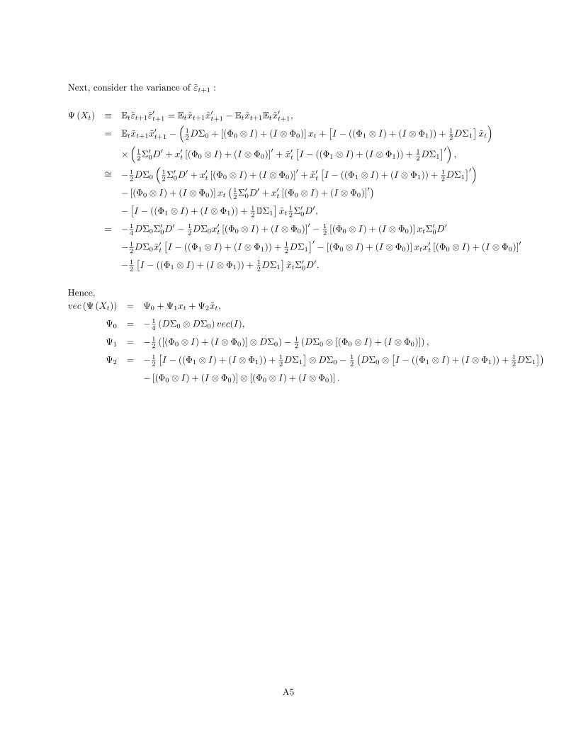
Next, consider the variance of εt+1 :

Ψ (Xt) ≡ Etεt+1ε′t+1 = Etxt+1x

′t+1 − Etxt+1Etx′t+1,

= Etxt+1x′t+1 −

(12DΣ0 + [(Φ0 ⊗ I) + (I ⊗ Φ0)]xt +

[I − ((Φ1 ⊗ I) + (I ⊗ Φ1)) + 1

2DΣ1

]xt

)×(

12Σ′0D

′ + x′t [(Φ0 ⊗ I) + (I ⊗ Φ0)]′+ x′t

[I − ((Φ1 ⊗ I) + (I ⊗ Φ1)) + 1

2DΣ1

]′),

∼= − 12DΣ0

(12Σ′0D

′ + x′t [(Φ0 ⊗ I) + (I ⊗ Φ0)]′+ x′t

[I − ((Φ1 ⊗ I) + (I ⊗ Φ1)) + 1

2DΣ1

]′)− [(Φ0 ⊗ I) + (I ⊗ Φ0)]xt

(12Σ′0D

′ + x′t [(Φ0 ⊗ I) + (I ⊗ Φ0)]′)

−[I − ((Φ1 ⊗ I) + (I ⊗ Φ1)) + 1

2DΣ1

]xt

12Σ′0D

′,

= − 14DΣ0Σ′0D

′ − 12DΣ0x

′t [(Φ0 ⊗ I) + (I ⊗ Φ0)]

′ − 12 [(Φ0 ⊗ I) + (I ⊗ Φ0)]xtΣ

′0D′

− 12DΣ0x

′t

[I − ((Φ1 ⊗ I) + (I ⊗ Φ1)) + 1

2DΣ1

]′ − [(Φ0 ⊗ I) + (I ⊗ Φ0)]xtx′t [(Φ0 ⊗ I) + (I ⊗ Φ0)]

′

− 12

[I − ((Φ1 ⊗ I) + (I ⊗ Φ1)) + 1

2DΣ1

]xtΣ

′0D′.

Hence,vec (Ψ (Xt)) = Ψ0 + Ψ1xt + Ψ2xt,

Ψ0 = − 14 (DΣ0 ⊗DΣ0) vec(I),

Ψ1 = − 12 ([(Φ0 ⊗ I) + (I ⊗ Φ0)]⊗DΣ0)− 1

2 (DΣ0 ⊗ [(Φ0 ⊗ I) + (I ⊗ Φ0)]) ,

Ψ2 = − 12

[I − ((Φ1 ⊗ I) + (I ⊗ Φ1)) + 1

2DΣ1

]⊗DΣ0 − 1

2

(DΣ0 ⊗

[I − ((Φ1 ⊗ I) + (I ⊗ Φ1)) + 1

2DΣ1

])− [(Φ0 ⊗ I) + (I ⊗ Φ0)]⊗ [(Φ0 ⊗ I) + (I ⊗ Φ0)] .

A5