tutorial: what would you like to do? - · pdf filelearn about the tutorial window this...
TRANSCRIPT

Tutorial: What Would You Like to Do?
Choose a lesson by clicking on its picture, link, or " ".
RockWare home page
Learn about this Tutorial/Help window. How to get around the help window.
Learn about the Borehole Manager and its tools. Create 2D and 3D log & interpolated diagrams, compute volumes.
Learn about the Utilities datasheet and its tools.
Learn about the EarthApps datasheet and its tools.
Learn about the RockPlot2D window and its tools. Open, combine, edit, export maps.
Learn about the RockPlot3D window and its tools. Open, combine, manipulate, export 3D images.
Learn about the ReportWorks window and its tools. Insert RockWorks images, bitmaps, legends.

Learn About the Tutorial Window
This RockWorks tutorial is displayed in the main RockWorks "Help" window.
Navigation Buttons:
Resizing/Repositioning this Window:
To move this window, simply grab its upper-most title bar (which reads "RockWorks Help") and drag it out of the way. To resize this window, position your mouse pointer on any edge (the pointer will change shape to an "<->"), click, and drag. To resize the left and right panes, drag the center divider.
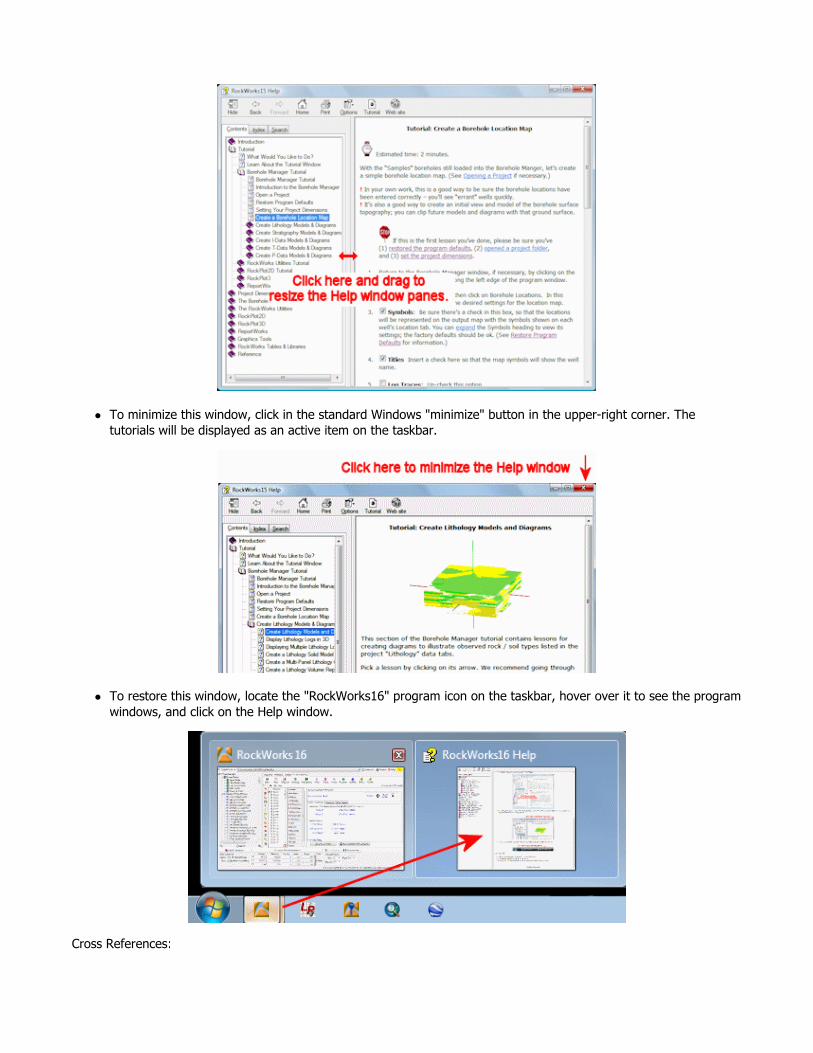
To minimize this window, click in the standard Windows "minimize" button in the upper-right corner. The tutorials will be displayed as an active item on the taskbar.
To restore this window, locate the "RockWorks16" program icon on the taskbar, hover over it to see the program windows, and click on the Help window.
Cross References:

Click on underlined items ("hyperlinks") to jump to their topics. Use hyperlink arrows to jump to their topics. The Help icon tells you where to find more information in the main Help section.
Back to main menu
RockWare home page
Tutorial: Borehole Manager
Choose a lesson by clicking on its " " or picture or link.
Introduction to the Borehole Manager.
Open a Project.
Restore program defaults.
Set your project's output dimensions.
Create a borehole location map. Borehole locations and surface contours.
Create lithology diagrams. Logs, models, sections, volume reports.
Create stratigraphy diagrams. Logs, sections, surfaces, models, reports.
Create"I-Data" diagrams. Logs, models, sections, fences of interval-based (geochemistry, geotechnical) data.
Create "T-Data" diagrams.
Back to main menu
RockWare home page
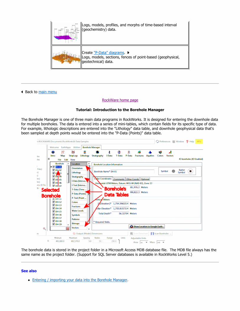
Tutorial: Introduction to the Borehole Manager
The Borehole Manager is one of three main data programs in RockWorks. It is designed for entering the downhole data for multiple boreholes. The data is entered into a series of mini-tables, which contain fields for its specific type of data. For example, lithologic descriptions are entered into the "Lithology" data table, and downhole geophysical data that's been sampled at depth points would be entered into the "P-Data (Points)" data table.
The borehole data is stored in the project folder in a Microsoft Access MDB database file. The MDB file always has the same name as the project folder. (Support for SQL Server databases is available in RockWorks Level 5.)
See also
Entering / importing your data into the Borehole Manager.
Logs, models, profiles, and morphs of time-based interval (geochemistry) data.
Create "P-Data" diagrams. Logs, models, sections, fences of point-based (geophysical, geotechnical) data.

Back to main menu | Next (Open Project)
RockWare home page
Tutorial: Open a Project
Estimated time: 2 minutes.
In this section, you will access a folder that was installed with the program. This folder contains Borehole Files and other sample files that have already been created. We will use these files throughout the tutorial; you can also refer to them when you are entering your own data.
1. First, access the Borehole Manager by clicking on its tab along the top of the program window.
2. Click on the Project Folder item right below the uppermost program title bar.

3. In the displayed window, click on the tutorial project folder we’ll be working with: First open the "RockWorks16 Data" folder (in "My Documents") and the "Samples" which is inside of that.

You will be returned to the main data window, with that folder displayed as the current project folder. All of the RockWorks-related files contained in this folder will be displayed in the Project Manager pane, along the left edge of the program window. The program will load the information for all of the boreholes in the current project into the data window.
You will see the listing of the borehole names in the Borehole File listing. The first borehole will be active and its data displayed in the data tabs.
4. Click on the Lithology button to see the observed rock/soil types, and then on the Stratigraphybutton to see the borehole’s formation depths.
5. Click on the other data buttons to see the data layout. Click here for a quick summary of the data tables.
6. Click on the borehole named "DH-03" and note that the contents of the data tables have changed to display the data for this particular well.
! All of the borehole data is stored in a Microsoft Access (MDB) database file in the project folder. The database file always has the same name as the project folder, so this database is named "Samples.mdb".
! In your own work, you can hand-enter the borehole data or import it from another source (LogPlot, Excel, etc.).
Borehole Data Overview
Back to main menu | Next (Restore Defaults)
RockWare home page
Tutorial: Restore Program Defaults
The purpose of this step is to reset all of the menu settings to their factory defaults. This will eliminate the need to

establish dozens and dozens of settings as you go through the tutorial.
!!! NOTE !!! This will set all of the menu options for this "Samples" project folder to the RockWare defaults. This means that if you have done a lot of work within this project, these settings will be lost. If this is a worry for you, you might consider the following: Before restoring the factory defaults, you can use the Preferences | Export Menu Settings option to store all of your current settings in a file that can later be imported back into the program using the Preferences | Import Menu Settings option.
Step-by-Step Summary
1. If you have just installed RockWorks (or a new version of RockWorks) you can skip this step because program defaults have already been established. (Click the Next button below.)
2. If you’ve been running RockWorks for a while (or if you aren’t sure), you should click on the Preferences menu and choose Reset Menu Settings.
3. Establish these menu options: Reset Global Settings: Uncheck this item. Reset Project Settings: Check this item. It will reset the project-specific settings to factory
defaults. 4. Click on the Process button at the bottom of the window. 5. Click Yes when prompted if you are sure that you wish to do this. 6. RockWorks will restore all of the settings of all of the menus to the project defaults.
Back to main menu | Next (Output Dimensions)
RockWare home page
Tutorial: Setting Your Output Dimensions
Each time you create a new project in RockWorks, you need to establish its geographic extents for RockWorks so that there will be consistency in how models and diagrams are dimensioned.
Here’s how you establish output dimensions:
1. Locate the Output Dimensions pane at the bottom of the program window.

Notes:
The Project Coordinate system and units, shown to the left, are already established. These are defined when a project folder is first created. For this Samples project, the borehole locations are entered in UTM meters (NAD-83, Zone 13), and the elevations and depth are also entered in meters. The Output (Model) Dimensions are the actual coordinate values that represent:
The extents of the project space: western, eastern, southern, northern, base elevation, and top elevation coordinate boundaries. The spacing of the nodes which will determine the density of grid models (XY) and solid models (XYZ) that you interpolate.
You can establish the Output (Model) Dimensions by typing in the coordinate values. Or you can use the Scan Boreholes button which is displayed to the right.
In your own work, the Scan Boreholes button is the easiest method to quickly establish the coordinate extents. For this project, we'll just have you confirm that the existing coordinates are correct.
2. Confirm the Min and Max Coordinates: Be sure these are set as shown here; you can type in the numbers as necessary.
3. Set the Node Spacing: a. X-Spacing: Be sure this prompt is set to: 5. This means that there will be a model node placed every 5
meters from west to east across the project space. This will generate 61 nodes from west to east in the models. You’ll note that when you change the Spacing setting, the number of nodes represented will be updated automatically.
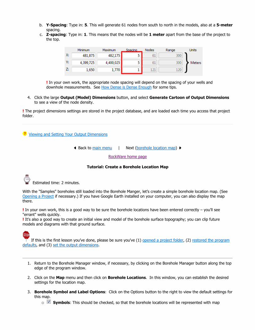
b. Y-Spacing: Type in: 5. This will generate 61 nodes from south to north in the models, also at a 5-meterspacing.
c. Z-spacing: Type in: 1. This means that the nodes will be 1 meter apart from the base of the project to the top.
! In your own work, the appropriate node spacing will depend on the spacing of your wells and downhole measurements. See How Dense is Dense Enough for some tips.
4. Click the large Output (Model) Dimensions button, and select Generate Cartoon of Output Dimensionsto see a view of the node density.
! The project dimensions settings are stored in the project database, and are loaded each time you access that project folder.
Viewing and Setting Your Output Dimensions
Back to main menu | Next (borehole location map)
RockWare home page
Tutorial: Create a Borehole Location Map
Estimated time: 2 minutes.
With the "Samples" boreholes still loaded into the Borehole Manger, let’s create a simple borehole location map. (See Opening a Project if necessary.) If you have Google Earth installed on your computer, you can also display the map there.
! In your own work, this is a good way to be sure the borehole locations have been entered correctly – you’ll see "errant" wells quickly.! It's also a good way to create an initial view and model of the borehole surface topography; you can clip future models and diagrams with that ground surface.
If this is the first lesson you’ve done, please be sure you've (1) opened a project folder, (2) restored the program defaults, and (3) set the output dimensions.
1. Return to the Borehole Manager window, if necessary, by clicking on the Borehole Manager button along the top edge of the program window.
2. Click on the Map menu and then click on Borehole Locations. In this window, you can establish the desired settings for the location map.
3. Borehole Symbol and Label Options: Click on the Options button to the right to view the default settings for this map.
Symbols: This should be checked, so that the borehole locations will be represented with map
symbols shown on each well’s Location datasheet. Borehole IDs: This should be checked, so that the map symbols will show the well name.
None of the other boxes should be checked at this time. Click OK to close this window.
4. Background Image: Un-check this option.
5. Surface Contours: Check this box. This will generate a grid model and contour map of the elevations declared at the boreholes’ surfaces. Expand the heading to access the surface map options.
Grid Name: IMPORTANT: Click to the right of the Grid Name prompt to view the name that will be assigned to the surface grid model. Be sure it reads Surface.RwGrd in the prompt box, and click the Save button. You will use this surface grid in later lessons. If you want to take a moment to drill down to the Gridding Options button or the Colored Intervals Color Schemes that are available, feel free to do so. These settings will be covered in other tutorial lessons.
6. Border: Check this box so that the map will be appended with coordinate labels. Expand this heading. Border Options: Click on the Options button. Border Dimensions: Be sure this setting, down at the bottom of the window, is set to Output Dimensions. There are a number of options under this heading that you can look at if you wish; again the factory defaults should be fine. Click OK to close the Border Options window.
7. Click the Process button at the bottom of the Borehole Location Map Options window to continue.
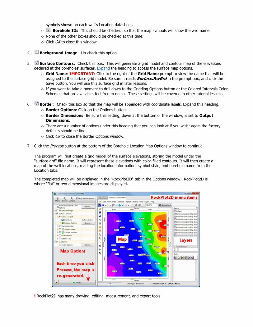
The program will first create a grid model of the surface elevations, storing the model under the "surface.grd" file name. It will represent these elevations with color-filled contours. It will then create a map of the well locations, reading the location information, symbol style, and borehole name from the Location tabs.
The completed map will be displayed in the "RockPlot2D" tab in the Options window. RockPlot2D is where "flat" or two-dimensional images are displayed.
! RockPlot2D has many drawing, editing, measurement, and export tools.
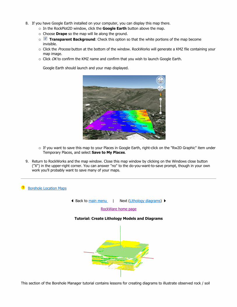
8. If you have Google Earth installed on your computer, you can display this map there. In the RockPlot2D window, click the Google Earth button above the map. Choose Drape so the map will lie along the ground.
Transparent Background: Check this option so that the white portions of the map become invisible. Click the Process button at the bottom of the window. RockWorks will generate a KMZ file containing your map image. Click OK to confirm the KMZ name and confirm that you wish to launch Google Earth.
Google Earth should launch and your map displayed.
If you want to save this map to your Places in Google Earth, right-click on the "Rw2D Graphic" item under Temporary Places, and select Save to My Places.
9. Return to RockWorks and the map window. Close this map window by clicking on the Windows close button ("X") in the upper-right corner. You can answer "no" to the do-you-want-to-save prompt, though in your own work you’ll probably want to save many of your maps.
Borehole Location Maps
Back to main menu | Next (Lithology diagrams)
RockWare home page
Tutorial: Create Lithology Models and Diagrams
This section of the Borehole Manager tutorial contains lessons for creating diagrams to illustrate observed rock / soil
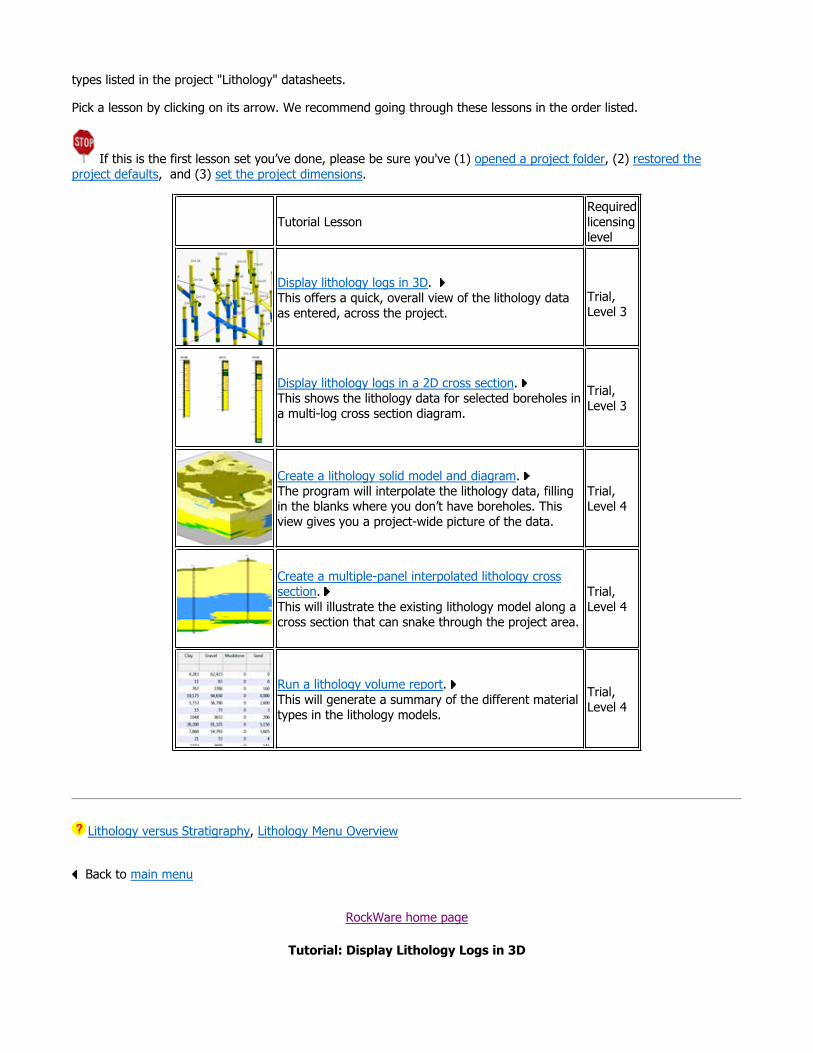
types listed in the project "Lithology" datasheets.
Pick a lesson by clicking on its arrow. We recommend going through these lessons in the order listed.
If this is the first lesson set you’ve done, please be sure you've (1) opened a project folder, (2) restored the project defaults, and (3) set the project dimensions.
Lithology versus Stratigraphy, Lithology Menu Overview
Back to main menu
RockWare home page
Tutorial: Display Lithology Logs in 3D
Tutorial LessonRequired licensing level
Display lithology logs in 3D. This offers a quick, overall view of the lithology data as entered, across the project.
Trial,Level 3
Display lithology logs in a 2D cross section. This shows the lithology data for selected boreholes in a multi-log cross section diagram.
Trial,Level 3
Create a lithology solid model and diagram. The program will interpolate the lithology data, filling in the blanks where you don’t have boreholes. This view gives you a project-wide picture of the data.
Trial,Level 4
Create a multiple-panel interpolated lithology cross section. This will illustrate the existing lithology model along a cross section that can snake through the project area.
Trial,Level 4
Run a lithology volume report. This will generate a summary of the different material types in the lithology models.
Trial,Level 4

Estimated time: 4 minutes.
In this lesson, you will get a quick view of all of the lithology data as entered for the project's boreholes. You will look at how the data is entered, and you will generate a 3D diagram representing the borehole lithology logs.
1. Be sure the "Samples" folder is still the current project folder (see Open a Project for information).
2. In the borehole file listing along the left side of the Borehole Manager, click on the borehole named "DH-01" to make it active.
3. Click on the Lithology button to view the lithologic data for this hole.
Note how the lithologic intervals are noted with a top and bottom depth, and a lithology "keyword". RockWorks lets you enter your rock/soil types using regular words like "silt" or "sand" or "interbedded sandstone and siltstone." In order to know what "interbedded sandstone and siltstone" is, the program relies on a reference library called a Lithology Types Table. This is created by the user. A Lithology Types Table is created for each project that has lithology information. We’ll look at this in a minute.
4. Click on another borehole name in the list to the left, and you’ll see the information listed in its Lithology datasheet.
Note also how the rock types can repeat – sand, clay, gravel, clay, sand - within a single borehole. Rock types that don’t show organized layering need to be entered into RockWorks as lithology. ("Stratigraphy" by contrast assumes defined layers that are consistent in order between holes and don’t repeat within a borehole. See the lessons on Stratigraphy diagrams for more information.)

5. Look at the project's Lithology Types Table: a. Click on the Lithology Types button that sits above the lithology data listings.
Note that you can also access the Lithology Types table using the Project Manager pane along the left edge of the program window, in the Project Tables | Types Tables grouping:
The program will display this project's lithology types.

A quick summary:
G-Value: Lists the numeric value to be assigned to each rock type. As RockWorks creates a solid model of the rock types, the nodes will be assigned these numeric values rather than the words "clay" or "gravel". In the final model, then, all Sand zones will be coded with a "5.0", Silts with a "4.0", Clays with a "3.0", and so on. We'll review this in a later lesson when you create a model of the lithology across the study area. Keyword: The rock types in this project. Pattern: The specific pattern in specific colors for the rock type. Fill Percent: Defines how much of the available space the pattern block should occupy in strip logs (less than 100% can show erosion, weathering). Density: The rock density - used only for computing mass. Show in Legend: Used to specify whether the material is to be included in the diagram legends. Un-checking an item doesn't remove it from the table itself, just from any subsequent legends that are created. To add a row to the listing, just click in the lowest existing row and press the down-arrow key on your keyboard. To delete a row from the listing, click in the row and type Ctrl+Del.
You can click on G-Value column heading to sort on those numbers, or the Keyword column heading to sort on the names.
b. Click on the OK button to close the Lithology Types Table.
6. Let’s create the 3D log diagram. Back at the Borehole Manager, click on the Striplogs menu at the top of the window, and select the 3-Dimensional | Multiple Logs menu option.
This window has several sections:The left side is where general diagram settings are established.The Instructions pane displays reference information about the settings. You'll find this in most of the RockWorks program windows.The 3D Striplog Designer tab is where you establish the log-specific settings. In this window:
The left pane is where you choose what type of data is to be displayed in the logs (the Visible Items). The upper-right pane is where you see a plan-view Preview of the active log items. You can drag the

items to adjust their relative placement. The lower-right pane displays specific Options for the Visible Item that you click on.
a. Establish the general diagram settings in the left pane.
Clip (Truncate Logs): Uncheck this.
Reference Cage: Uncheck this. Include Lithology Legend: Check this item so that the lithology background colors and the
rock type names will be included in the diagram. If you’d like to see the settings, you can expandthis heading.
Include Stratigraphy Legend: Uncheck this.
Include Well Construction Legend: Uncheck this.
Include Aquifer Legend: Uncheck this.
b. Click on the 3D Striplog Designer tab.
Choose the items you want to see in the logs by inserting a check-mark in the following items in the Visible Items section of the window:
c. Title: The drill hole name will plot above the logs. Lithology: The logs will contain a column illustrating rock types with cylinders of colors. When
the Lithology column is selected, you'll see a yellow circle displayed in the plan-view Preview pane.
Adjust the size of the column by dragging on one of the corner handles. Note the Column Radius setting in the lower-right Options pane. As you resize the circle, the Radius setting will be updated. Drag the yellow lithology circle until the Column Radius is about 1.0.! You can simply type 1.0 into the Column Radius prompt, if you prefer. Adjust the placement of the column relative to the axis of the log by dragging the circle in the Preview pane. Be sure the yellow lithology circle is on the center of the log axis.! You can simply type 0.0 into the Offset Distance prompt, if you prefer.
None of the other Visible Items should be checked.
7. Click the Process button at the bottom Options window to proceed.
The program will create a strip log for each borehole, including well name and lithology column, and these logs will be displayed in a new RockPlot3D display tab. ! Each time you click the Process button, the 3D display will be regenerated.
This is a true 3D viewing program – let’s take just a moment to look around.
The image is displayed in the pane to the right, and the image components as well as the standard reference items are listed in the "data" pane to the left of the image. (You can swap the position of the image and data panes using the << or >> buttons above the "linked file list.")
8. Enlarge the plot window by hiding the far left menu pane: click on the small "-" button in the middle of the divider.
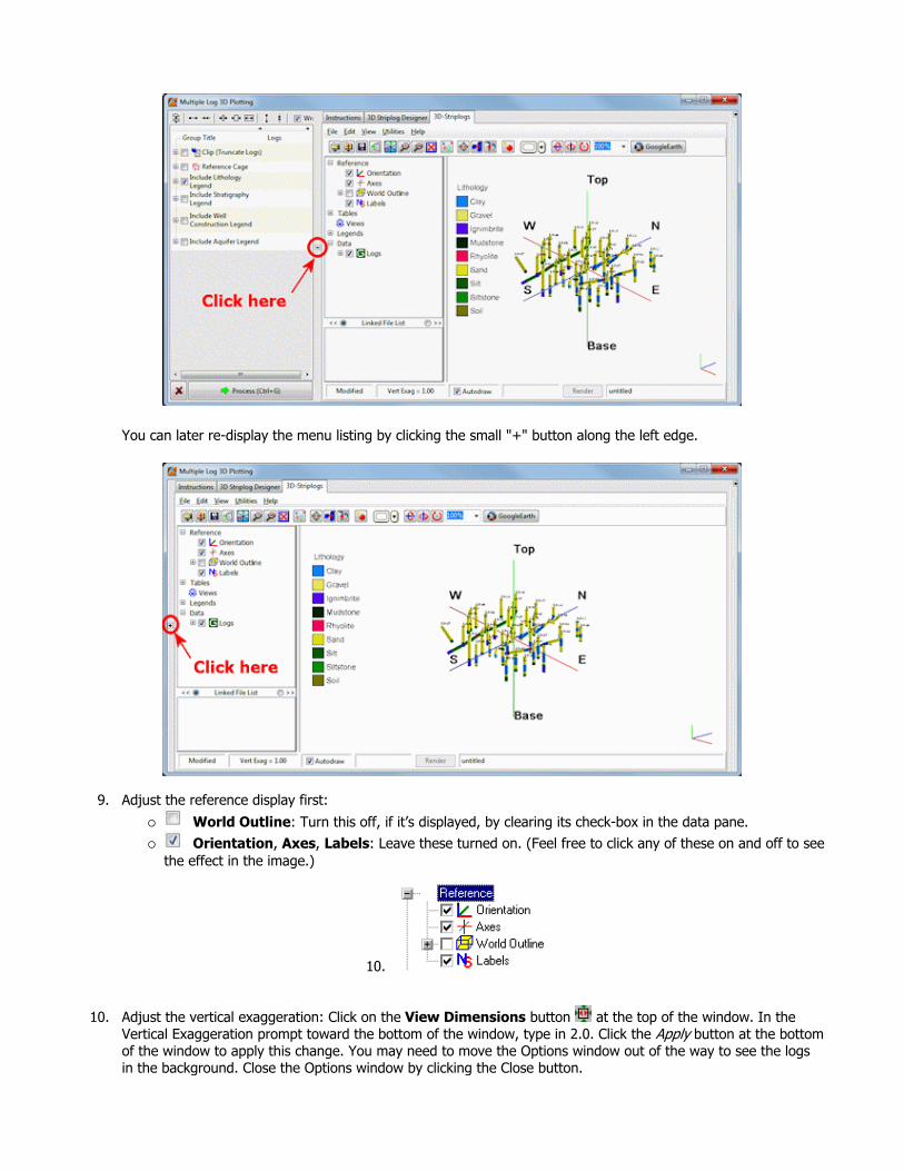
You can later re-display the menu listing by clicking the small "+" button along the left edge.
9. Adjust the reference display first:
World Outline: Turn this off, if it’s displayed, by clearing its check-box in the data pane. Orientation, Axes, Labels: Leave these turned on. (Feel free to click any of these on and off to see
the effect in the image.)
10.
10. Adjust the vertical exaggeration: Click on the View Dimensions button at the top of the window. In the Vertical Exaggeration prompt toward the bottom of the window, type in 2.0. Click the Apply button at the bottom of the window to apply this change. You may need to move the Options window out of the way to see the logs in the background. Close the Options window by clicking the Close button.

11. Rotate the image: The default viewing operation is "rotate" (see the button depressed in the toolbar ). Left-click and hold anywhere in the log display and drag to the left or right, up or down and see how the display rotates. Release the mouse button when you are done. Rotate the image again if you wish. Note that the log depth labels always face you even after rotating!
12. To restore the view to a fixed viewpoint, choose one from the View | Above, View | Below, or View | Compass Points options. (This can be helpful if you get your image turned upside-down.)
Tip: If you customize the display using a viewpoint that you like, use the View | Add View option to save the viewpoint for later retrieval with a double-click.
13. Click on the Pan button in the toolbar to reposition the image in the window. This tool is useful if you use the zoom in tool.
14. Turn on/off logs or log items: Notice the only listing under "Data" in the data pane is a "Group" named "Logs". Expand the Logs item (by clicking on its "+" button) to see the individual boring names. You can turn entire logs on and off simply by checking/clearing their respective check-boxes. Try this for a few borings.
15. In addition, if you expand an individual borehole in the data list, you’ll see its title and lithology intervals. These, also, can be turned on and off for each well. And, if you expand the Lithology for an individual borehole, you can turn on and off display of specific depth intervals.
16. ! You might be wondering why the 3D log "tubes" don't contain any lithology patterns. Note that RockWorks displays only the background color in 3D logs and other diagrams, because of the OpenGL 3D graphics engine. In the next lesson, you’ll create a 2D strip log which will display lithology pattern designs.
16. Adjust the legend: Expand the Legends item (above the log data items) in the data pane. Double-click on the Lithology item. This window can be used to move the legend up/down/left/right, and to scale the legend. It also notes the project’s Lithology Types Table as the source for its colors and labels.

Try changing the placement from the Left Side to the Right Side and click Apply. Change it back to the Left Side and click Apply again. Click Close to close the Legend Options window.
17. Save this 3D log image: Click on the File menu - the menu bar is above the viewing pane - and choose the Save As command. In the displayed window, type in this name: lithology logs and click the Save button. RockPlot3D will save this information on disk under that name, with a file name extension .Rw3D. In later lessons, you can append these logs to other 3D diagrams.
18. Close the RockPlot3D window by clicking in the Windows Close button .
3D Logs
Back to Lithology menu | Next (log section)
RockWare home page
Tutorial: Display Multiple Lithology Logs in a 2D Cross-Section
Estimated time: 4 minutes.
In this lesson, you will be creating an image representing the lithology data in multiple logs in the Samples project, selected along a multi-log cross section trace.
1. Back at the main Borehole Manager window, click on the Striplogs menu, and then click on 2-Dimensionaland pick the Section option from the pop-up menu.
2. Establish the section options:These are found in the left pane of the Lithology Section window. Plot Striplogs: Check this.
Borehole Spacing: Expand this heading if necessary and be sure that this is set to Distance between Collar Locations.
Plot Correlations: Uncheck this. (In later lessons you will activate Stratigraphy, I-Data or P-Data panels.)
Hang Section on Datum: Uncheck this.
or Plot Surface Profile: If you completed the borehole map section of the tutorial (jump back), insert a check in the Plot Surface Profile option. This is used to display a selected surface in the cross section plot. If you DID NOT complete that lesson, leave this un-checked.
Expand this heading to access the Surface Profile Options button. Grid Model: Click on the browse button to the right of the prompt and select the .RwGrd file representing the ground surface, named surface.RwGrd and click the Open button. Line Style & Color: Click here to set the line style to red, medium thickness. Smoothing factor can be set to 1. Click OK to close the optons window.
Show Faults: Uncheck this.
Perimeter Annotation Options: These options determine text and lines that will plot around the perimeter of the profile. Click on this button to view the options; the factory defaults should be fine. See Restore Default Settings if you need more information about setting the factory defaults.

! In your own work the Intended Vertical Exaggeration Factor can be very helpful for good diagram proportions if you have a large, flat study area and will stretch your cross sections for readability.
Create Location Map: Check this item. This will create a small map that shows the location of the profile "cut" in the study area. Expand this heading to change:
Append Map to Profiles and Sections: Check this option. Expand this heading and be sure the Size setting is set to Medium.
Display Map as Separate Diagram: Uncheck this option.
Legends: Click on the Options button Lithology: Check this item. Uncheck the other legend options.
Clip (Vertically Truncate) Diagram: Uncheck this.
3. Establish the striplog options: Now you need to set up how the logs within the cross section will look. Click on the 2D Striplog Designer tab, to the right.
The program will display the 2D log designer window. This window has three main sections: The left pane is where you choose what type of data is to be displayed in the logs (the Visible Items). The upper-right pane is where you see a Preview of the active log items. You can drag the items to adjust their relative placement. The lower-right pane displays specific Options for the Visible Item that you click on.
a. Choose the items you want to see in the logs by inserting a check-mark in the following items in the Visible Items section of the window:
Title: The drill hole name will plot above the logs. Depths: The logs will be labeled with depth tick marks and labels. Lithology: The logs will contain a column illustrating rock types with graphic patterns and colors.
None of the other options, including Text, should be checked.
b. Adjust the arrangement of the visible log items: You should see four items in the upper Preview pane: title, depth bar, log axis, and lithology patterns.
Practice clicking on an item, holding down the mouse button, and dragging it to the left or right in the preview. Try getting the items aligned in the following order:
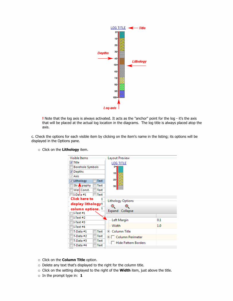
! Note that the log axis is always activated. It acts as the "anchor" point for the log - it's the axis that will be placed at the actual log location in the diagrams. The log title is always placed atop the axis.
c. Check the options for each visible item by clicking on the item's name in the listing; its options will be displayed in the Options pane.
Click on the Lithology item.
Click on the Column Title option. Delete any text that's displayed to the right for the column title. Click on the setting displayed to the right of the Width item, just above the title. In the prompt type in: 1

! All log item sizes are expressed as a percent of the dimensions of the project, so the width of these logs will be about 1% of the project dimensions.
4. Next, pick the boreholes to display. Click on the Section Selection Map tab.
Click on the Clear button at the top of the panel-picking window. The program remembers your cross section traces from session to session; this will clear any old traces from memory. Next, locate the hole titled "DH-31" (top, just left of the center) and click on it. It will be marked with a red "X". Locate hole "DH-18" south8 of "31" and click on it. A line will be drawn between the holes. Locate hole "DH-21" south of "18" and click on it.! If you make a mistake, click the Undo button to undo the last pick or the Clear button to clear the slate for starting over. Click on "DH-36," "DH-01," "DH-35", and "DH-13" continuing the cross section southward through the project area. You should see a trace like this:
5. Process: Click the Process button at the bottom of the Lithology Section window when you are ready to create the log section plot.
The program will create strip logs of each of the selected borings using the selected settings. The logs will be spaced proportionally to their distance from each other on the ground.In addition, it will create a map that displays the location of the section slice within the study area and append it to the cross section.
The completed log section will be displayed in a RockPlot2D tab in the Options window. RockPlot2D is
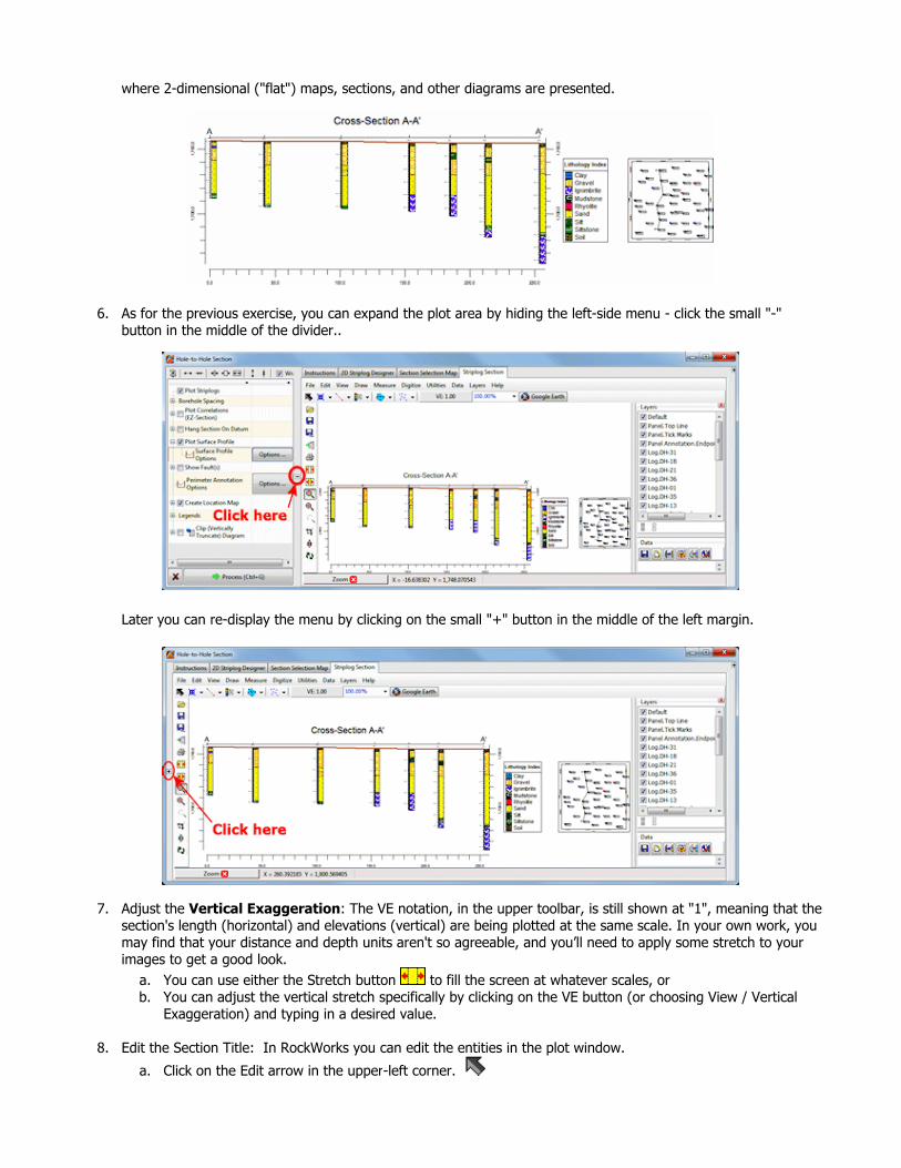
where 2-dimensional ("flat") maps, sections, and other diagrams are presented.
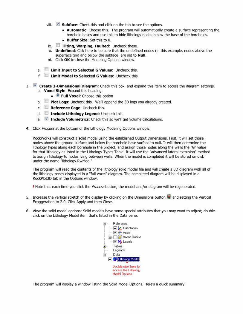
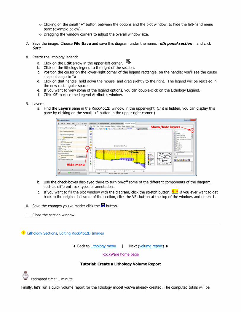
6. As for the previous exercise, you can expand the plot area by hiding the left-side menu - click the small "-" button in the middle of the divider..
Later you can re-display the menu by clicking on the small "+" button in the middle of the left margin.
7. Adjust the Vertical Exaggeration: The VE notation, in the upper toolbar, is still shown at "1", meaning that the section's length (horizontal) and elevations (vertical) are being plotted at the same scale. In your own work, you may find that your distance and depth units aren't so agreeable, and you’ll need to apply some stretch to your images to get a good look.
a. You can use either the Stretch button to fill the screen at whatever scales, or b. You can adjust the vertical stretch specifically by clicking on the VE button (or choosing View / Vertical
Exaggeration) and typing in a desired value.
8. Edit the Section Title: In RockWorks you can edit the entities in the plot window.
a. Click on the Edit arrow in the upper-left corner.

b. Double-click on the Cross Section A - A' title c. Click in the color box and change the color to red. d. Click the Apply button. This change will be displayed in the plot window. e. Click Close to close the Text Attributes window.
9. Save these images for later work in the ReportWorks program, where you can create a nice layout of the log profile and the section location map.
a. With the cross section still displayed in the RockPlot window, click on the File menu above the plot window, chooseSave, and type in the name: lith log section and click Save. The program will save this image in its own ".Rw2D" file format.
b. You can close this RockPlot window by clicking in the standard Windows close-window button .
10. If you’d like to do the ReportWorks lesson at this time, click here.
11. Otherwise, continue on with the lithology diagram lessons, below.
See also: RockPlot2D tutorial
Displaying Multiple Logs in a 2D Hole to Hole Section, Hole to Hole Sections versus Profile Sections
Back to Lithology menu | Next (3D Lithology Model)
RockWare home page
Tutorial: Create a Lithology Solid Model and Diagram
Estimated time: 6 minutes.
Now we will jump from the Striplogs menu, where we plotted observed data in log diagrams, to the Lithology menu, where the lithology data will be interpolated into a continuous model.
In this lesson, you will create a solid model and 3-dimensional block diagram of lithology. The program will look at the observed lithology intervals, that you viewed in logs and log sections already, and extrapolate the lithology throughout the project, outward from the boreholes. This modeling process basically "fills in the blanks" between the logs. RockWorks uses a specific lithology modeling algorithm to do this extrapolation. The images below show how you might conceptualize the transformation between observed data which is displayed in logs, and interpolated data which displayed as a solid diagram.
! You must be using RockWorks in Trial mode, or have a Level 4 or Level 5 license to run this modeling program.

Before continuing, be sure you have opened the sample project, established the project dimensions and created 3D logs, as discussed in earlier lessons.
1. With the Samples data still loaded into the Borehole Manager, click on the Lithology menu, and select the Model option.
2. Lithology Modeling Options: Establish the modeling settings:
a. Create New Model: Click here to tell the program that we want to interpolate a new solid lithology model. Expand this item.
b. Create Filtering/Sampling Report: Uncheck this.
c. Lithology Model Name: Click to the right and type in: lithology and click the Save button. This will be the name assigned to the solid model to be created. The file will be given a .RwMod file name extension.
d. Modeling Options: Click the Options button to access a large number of modeling settings. i. Algorithm: Be sure this is set to Lateral Blending. This is a unique algorithm which "bleeds"
lithology types outward from the boreholes into a solid model. Interpolate Outliers: Check this.
ii. Model Dimensions: This option, to the right, should be set to Based on Output Dimensions.! In your own work, we recommend you "hardwire" solid and grid models to the Output Dimensions so that they are consistent. However, the program does offer the option to vary the model dimensions, under the Variable Dimensions heading.
Confirm Model Dimensions: This item can be left unchecked (though in your own work, this is a handy way to double-check the model extents and node spacing).
iii. Decluster: This can be checked.
iv. Add Points: Uncheck this. In your own work, this can be a handy way to add control points to the modeling.
v. Smoothing: This can be checked.
vi. Polygon: Uncheck this. vii. Superface: Check this, and click on the tab to see the options.
Automatic: Choose this option. The program will automatically create a surface representing the borehole tops (e.g. ground surface) and use this to hide (set to "null") lithology model nodes above ground. Buffer Size: Set this to 0.
viii. Subface: Check this and click on the tab to see the options. Automatic: Choose this. The program will automatically create a surface representing the borehole bases and use this to hide lithology nodes below the base of the boreholes. Buffer Size: Set this to 0.
ix. Tilting, Warping, Faulted: Uncheck these. x. Undefined: Clck here to be sure that the undefined nodes (in this example, nodes above the
superface grid and below the subface) are set to Null. xi. Click OK to close the Modeling Options window.
e. Limit Input to Selected G Values: Uncheck this.
f. Limit Model to Selected G Values: Uncheck this.
3. Create 3-Dimensional Diagram: Check this box, and expand this item to access the diagram settings. a. Voxel Style: Expand this heading.
Full Voxel: Choose this option
b. Plot Logs: Uncheck this. We’ll append the 3D logs you already created. c. Reference Cage: Uncheck this.
d. Include Lithology Legend: Uncheck this. e. Include Volumetrics: Check this so we'll get volume calculations.
4. Click Process at the bottom of the Lithology Modeling Options window.
RockWorks will construct a solid model using the established Output Dimensions. First, it will set those nodes above the ground surface and below the borehole base surface to null. It will then determine the lithology types along each borehole in the project, and assign those nodes along the wells the "G" value for that lithology as listed in the Lithology Types Table. It will use the "advanced lateral extrusion" method to assign lithology to nodes lying between wells. When the model is completed it will be stored on disk under the name "lithology.RwMod."
The program will read the contents of the lithology solid model file and will create a 3D diagram with all of the lithology zones displayed in a "full voxel" diagram. The completed diagram will be displayed in a RockPlot3D tab in the Options window.
! Note that each time you click the Process button, the model and/or diagram will be regenerated.
5. Increase the vertical stretch of the display by clicking on the Dimensions button and setting the Vertical Exaggeration to 2.0. Click Apply and then Close.
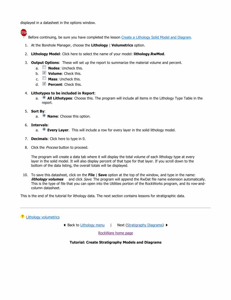
6. View the solid model options: Solid models have some special attributes that you may want to adjust; double-click on the Lithology Model item that’s listed in the Data pane.
The program will display a window listing the Solid Model Options. Here’s a quick summary:

Color scheme: Since the colors are specific to the colors defined in the Lithology Types Table, RockWorks will list that as source. In other tutorials you’ll see geochemistry solid models displayed differently, such as color-coded from cold-to-hot. Smoothing: Smooth (default) blends the colors in the display while Flat displays abrupt color changes. Draw Style: Default is Voxels. You might try changing the display to Solid (a similar view, but faster to render), Wire Frame or Points to see the effect. Click the Apply button at the bottom of the window to make any changes you set take affect. Opacity: You’ll see this one in most 3D Options windows. You can make the block more transparent by reducing the percent opacity shown here. Again, use Apply to see changes take effect. Filter: This allows you to see only selected G values in the block. See #11 below. Slices: This allows you to see specific slices in the block. See #12 below.
7. If you have a minute, you should go through the next few steps to learn some of the ins and outs of viewing solid model voxel diagrams. If you are in a hurry, you can review these lessons later in the dedicated RockPlot3D tutorial.
8. Rotate: Leave the Solid Model Options window open while you Rotate or Pan the image display. (You have full control over the image display even when one or more Options windows are open.) Or, use a viewpoint in the View | Above or Below or Compass Points tools to return to a pre-set view.
9. Expand the Lithology Volumetrics heading in the data pane. There you'll see a listing of all of the material types in the project, and their volumes in the current model (see the items circled in blue below). You will also see the "G" values for each rock type (circled in red) - we'll use this in the next step. You assign a "G" value for each rock type in the Lithology Types table, and the program uses that value to represent the material in the solid model.
10. Invoke a filter: Click back in the Solid Model Options window. a. Filter Enabled: Check this.
1. In the Low prompt type in 3.0 and in the High type in 5.0, and press Apply to see only those areas where the silt (G=3), sand (G=4) and gravel (G=5) materials are present. If the Show Volume check-box is checked, the program will display right there in the window the total volume of these materials in the current model.
2. Try this one more time, changing the Low value to 6 and the High value to 7 and clicking Apply, so that the mudstone and siltstone materials are displayed. You can click back into the image and rotate as you wish for a different view. Note that the Show Volume value is updated to reflect the sand & gravel volume.

! In your own work, you may decide to have fewer lithology types, or more, depending on the level of detail you're after. The G values can be grouped by gradational rock types, as they are here, or completely random. The G values can be integers use decimal places.
b. Filter Enabled: Now, uncheck this. Click Apply.
11. Insert some slices: Another means of visualizing the inside of the lithology model is to insert some slice planes. a. Horizontal: Click in this button in the Slices section of the window. This tells the program that you
want to insert a horizontal slice. The slider bar will show the elevation at the base of the model to the left and the elevation at the top of the model at the right. Drag the slider bar to the right, to an elevation of around 1715, and click the Add button.
b. The program will insert a slice in the Data listing in the data pane. Hmmm – nothing shows up in the image pane. We need to hide the voxels to see the slice.
c. Draw Style: Choose Hidden, and click Apply. Aha, there’s the horizontal slice. d. Add another horizontal slice by dragging the slider bar to an elevation of 1740 and click the Add button. e. Repeat this process if you would like to insert vertical North-South or East-West slices. For these entities,
the slider bar will represent south-to-north or west-to-east coordinates. f. If you want to remove a slice, right-click on the slice’s name in the Data listing, and choose Delete.
12. Close all of the Options windows that may be open, by clicking the Close button in each.
13. Save this view: Choose the File|Save As command and type in the name: lithology solid and click the Savebutton. This view will be saved under this name, with an ".Rw3D" file name extension.
14. Append your logs: Finally, if you want to append your 3D strip logs from an earlier lesson to your slice display, choose the File | Append menu option, choose the file "lithology logs.Rw3D" and click Open. You will see your 3D strip logs displayed along with the model slices.
15. Save this combined view: Choose File|Save, and the new entities will be saved in this view.
16. Close this RockPlot3D window by clicking in its upper-right Close box.
Solid modeling reference, Creating lithology models
Back to Lithology menu | Next (interpolated section)
RockWare home page
Tutorial: Create a Multi-Panel Lithology Cross-Section

Estimated time: 3 minutes.
In this lesson, you will create a multi-paneled set of section panels using the same lithology model you created in the previous lesson. The instructions below are written with the assumption that you have completed that lesson, as well as the lesson on log sections. You'll be using the same settings for the lithology cross section.
1. Click on the Lithology Menu and choose Section.
2. Set up the section options: a. Lithology Modeling Options: Establish the modeling settings.
Use Existing Model: Click in this button to tell the program you want to use the same, existing lithology model file. Expand this heading if necessary. Model Name: Click here to select the file named "lithology.RwMod", created in the previous lesson.
b. Fill Options: Fill Background: Check this box to be sure that the background colors for the rock types are
displayed in the section. Plot Patterns: Check this box to display the pattern designs as well.
c. Confirm the following settings are still established, from the log section lesson: Lithology Legend. Plot Logs: The program will append 2D logs to the section panels.
or Plot Surface Profile: This option can be either checked or not, as per the log section lesson.
Show Faults: Turn this option off. Perimeter Annotation Options: The defaults from the earlier lesson should work.
Create Location Map.
3. Check the striplog options: These should still be set up as they were for the log section; if you want to review the 2D log settings you can click on the 2D Striplog Designer tab to the right.
4. Check the selected boreholes: These should also still be set up as they were for the log section. To verify the placement of the section trace, click on the Section Selection Map tab to the right.
5. Process: When you're ready to proceed, click the Process button at the bottom of the window.
The program will read the existing solid model (lithology.RwMod) and extract panels along the indicated cross-section trace. It will build them into a continuous cross section diagram, with the indicated perimeter annotation and surface profile line. The lithology logs will be appended to the section diagram. The completed diagram will be displayed in a RockPlot2D tab in the options window.
6. Resize the plot window as necessary: You can adjust the display by:
Clicking on the small "+" button between the options and the plot window, to hide the left-hand menu pane (example below). Dragging the window corners to adjust the overall window size.
7. Save the image: Choose File|Save and save this diagram under the name: lith panel section and click Save.
8. Resize the lithology legend:
a. Click on the Edit arrow in the upper-left corner. b. Click on the lithology legend to the right of the section. c. Position the cursor on the lower-right corner of the legend rectangle, on the handle; you'll see the cursor
shape change to d. Click on that handle, hold down the mouse, and drag slightly to the right. The legend will be rescaled in
the new rectangular space. e. If you want to view some of the legend options, you can double-click on the Lithology Legend. f. Click OK to close the Legend Attributes window.
9. Layers: a. Find the Layers pane in the RockPlot2D window in the upper-right. (If it is hidden, you can display this
pane by clicking on the small "+" button in the upper-right corner.)
b. Use the check-boxes displayed there to turn on/off some of the different components of the diagram, such as different rock types or annotations.
c. If you want to fill the plot window with the diagram, click the stretch button. If you ever want to get back to the original 1:1 scale of the section, click the VE: button at the top of the window, and enter: 1.
10. Save the changes you've made: click the button.
11. Close the section window.
Lithology Sections, Editing RockPlot2D Images
Back to Lithology menu | Next (volume report)
RockWare home page
Tutorial: Create a Lithology Volume Report
Estimated time: 1 minute.
Finally, let’s run a quick volume report for the lithology model you’ve already created. The computed totals will be
displayed in a datasheet in the options window.
Before continuing, be sure you have completed the lesson Create a Lithology Solid Model and Diagram.
1. At the Borehole Manager, choose the Lithology | Volumetrics option.
2. Lithology Model: Click here to select the name of your model: lithology.RwMod.
3. Output Options: These will set up the report to summarize the material volume and percent. a. Nodes: Uncheck this. b. Volume: Check this. c. Mass: Uncheck this. d. Percent: Check this.
4. Lithotypes to be included in Report: a. All Lithotypes: Choose this. The program will include all items in the Lithology Type Table in the
report.
5. Sort By: a. Name: Choose this option.
6. Intervals: a. Every Layer. This will include a row for every layer in the solid lithology model.
7. Decimals: Click here to type in 0.
8. Click the Process button to proceed.
The program will create a data tab where it will display the total volume of each lithology type at every layer in the solid model. It will also display percent of that type for that layer. If you scroll down to the bottom of the data listing, the overall totals will be displayed.
10. To save this datasheet, click on the File | Save option at the top of the window, and type in the name: lithology volumes and click Save. The program will append the RwDat file name extension automatically. This is the type of file that you can open into the Utilities portion of the RockWorks program, and its row-and-column datasheet.
This is the end of the tutorial for lithology data. The next section contains lessons for stratigraphic data.
Lithology volumetrics
Back to Lithology menu | Next (Stratigraphy Diagrams)
RockWare home page
Tutorial: Create Stratigraphy Models and Diagrams

This section of the Borehole Manager tutorial contains lessons for creating diagrams to illustrate interpreted stratigraphic units listed in the project "Stratigraphy" data tables.
If you have already done the lithology lessons, many of these procedures will be very much the same. The images will look different, however, because they represent stratigraphic layers rather than observed lithologies.
Pick a lesson by clicking on its arrow. We recommend going through these lessons in the order listed.
If this is the first lesson set you’ve done, please be sure you've already (1) opened a project folder, (2) restored the program defaults, and (3) set the output dimensions.
Tutorial LessonRequired licensing level
Display stratigraphy logs in 3D. This offers a quick, overall view of the stratigraphy data as entered, across the project.
Trial,Level 3
Display stratigraphy logs in a 2D cross section. This shows the stratigraphy data for selected boreholes in a multi-log cross section diagram, with straight-line correlation panels.
Trial,Level 3
Create a 3D stratigraphic model. Here you will create surface models for the top and base of each formation and display them as a stratigraphic model in 3D.
Trial,Level 4
Create a modeled stratigraphic cross section. Using the surfaces interpolated above, we'll create an interpolated cross section.
Trial,Level 4
Create a 2D stratigraphic structure map. Create a plan-view contour map of a formation's elevations.
Trial,Level 4

See also: Lithology versus Stratigraphy
Back to main menu
RockWare home page
Tutorial: Display Stratigraphy Logs in 3D
Estimated time: 6 minutes.
In this lesson, you will get a quick view of all of the stratigraphy data as entered for the project's boreholes. You will look at how the data is entered, and you will generate a 3D diagram representing the borehole stratigraphy logs.
1. Be sure the "Samples" folder is still the current project folder (see Open a Project for information).
2. In the borehole file listing along the left side of the Borehole Manager, click on the borehole named "DH-04" to make it active.
3. Click on the Stratigraphy button to load the stratigraphic data for this hole.
Run a stratigraphy volume report. Compute the volume of each layer in the stratigraphic solid model.
Trial,Level 4

! Note how the stratigraphic units are noted with a top and bottom depth, and a formation name. Missing data can be left blank (as in the Leadville Ls base depth above) and there are a set of "rules" which can help fill in the blanks. You can enter your formations or layers using regular words like "limestone" or "Leadville Ls." In order to know formation order, and the colors and patterns to be used to represent them, the program relies on a reference library called a Stratigraphy Types Table. This is created by the user. A Stratigraphy Types Table is created for each project that has stratigraphy information. We’ll look at this in a minute.
4. Click on the borehole "DH-03" in the list to the left, and you’ll see the information listed in its Stratigraphy datasheet.
Note how the formations must be consistent in order between boreholes. The formations CANNOT repeat within a single borehole. ("Lithology" by contrast does not show organized layering. See the lessons on lithology diagrams for more information.)
If formations are missing from a particular borehole, you can either omit them altogether, or enter them with the same top and base as the formations above and below (and thus have zero thickness). The latter method allows for better pinching out of surfaces. See Missing Formations for more details.
5. Look at the project's Stratigraphy Types Table: a. Click on the Stratigraphy Types button that sits above the stratigraphy data listings.
You can also access the Stratigraphy Types table using the Project Manager pane along the left edge of the program window, in the Project Tables | Types Tables grouping.
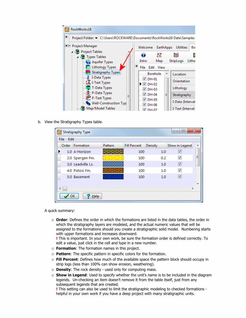
b. View the Stratigraphy Types table.
A quick summary:
Order: Defines the order in which the formations are listed in the data tables, the order in which the stratigraphy layers are modeled, and the actual numeric values that will be assigned to the formations should you create a stratigraphic solid model. Numbering starts with upper formations and increases downward.! This is important. In your own work, be sure the formation order is defined correctly. To edit a value, just click in the cell and type in a new number. Formation: The formation names in this project. Pattern: The specific pattern in specific colors for the formation. Fill Percent: Defines how much of the available space the pattern block should occupy in strip logs (less than 100% can show erosion, weathering). Density: The rock density - used only for computing mass. Show in Legend: Used to specify whether the unit's name is to be included in the diagram legends. Un-checking an item doesn't remove it from the table itself, just from any subsequent legends that are created.! This setting can also be used to limit the stratigraphic modeling to checked formations -helpful in your own work if you have a deep project with many stratigraphic units.

To add a row to the listing, just click in the lowest existing row and press the down-arrow key on your keyboard. To delete a row from the listing, click in the row and type Ctrl+Del.
c. Click on the OK button to close the Stratigraphy Types Table.
6. To create the 3D logs, click on the Striplogs menu, and then click on 3-Dimensional | Multiple Logs.
This window has several sections:The left side is where general diagram settings are established.The 3D Striplog Designer tab is where you establish the log-specific settings. In this window:
The left pane is where you choose what type of data is to be displayed in the logs (the Visible Items). The upper-right pane is where you see a plan-view preview of the active log items. You can drag the items to adjust their relative placement. The lower-right pane displays specific settings for the Visible Item that you click on.
a. Establish the general diagram settings in the left pane.
Clip (Truncate Logs Based on Elevation Range): Uncheck this. Reference Cage: Check this. A 3D grid of lines and coordinate labels will be included.
Include Lithology Legend: Uncheck this.
Include Stratigraphy Legend: Uncheck this. We'll add one interactively in RockPlot3D.
Include Well Construction Legend: Uncheck this.
Include Aquifer Legend: Uncheck this.
b. Click on the 3D Striplog Designer tab.
Choose the items you want to see in the logs by inserting a check-mark in the following items in the Visible Items section of the window:
Title: The drill hole name will plot above the logs. Stratigraphy: The logs will contain a column illustrating the stratigraphy units with
cylinders of colors. When the Stratigraphy column is selected, you'll see a green circle displayed in the plan-view Preview pane.
Adjust the size of the column by dragging on one of the corner handles. Note the Column Radius setting in the lower-right Options pane. As you resize the circle, the Radius setting will be updated. Drag the green stratigraphy circle until the Column Radius is about 1.0.! You can simply type 1.0 into the Column Radius prompt, if you prefer. Adjust the placement of the column relative to the axis of the log by dragging the circle in the Preview pane. Be sure the green stratigraphy circle is on the center of the log axis.! You can simply type 0.0 into the Offset Distance prompt, if you prefer.
None of the other Visible Items should be checked.

7. Click the Process button at the bottom Options window to proceed.
The program will create a strip log for each borehole, including well name and stratigraphy column, and it will build a labeled reference cage around the logs. The entire diagram will be displayed in a new RockPlot3D display tab. ! Each time you click the Process button, the 3D display will be regenerated.
The instructions below will take you on a quick tour of RockPlot3D. This lesson will cover different items than were highlighted in the lithology tutorial.
As you can see, the image is displayed in the pane to the right, and the image components and the standard reference items are listed in the pane to the left, called the "data tree."
8. Adjust the background color for the display, by clicking the color button in the toolbar above the image display and making a selection. The program will remember the background color you select from session to session.
9. Adjust the reference items in the upper portion of the window's data pane.
a. World Outline: Uncheck this - since there’s a reference grid in this image, the world outline is redundant.
b. Axes: Turn this item off.
10. Practice rotating the image. The default viewing operation is "rotate" (see the button depressed in the toolbar ). Left-click and hold anywhere in the log display and drag to the left or right, up or down and see how the
display rotates. Release the mouse button when you are done. Rotate the image again if you wish.
11. Set the view to a fixed viewpoint by clicking on the View | Above option. From the pop-up list, select North-East. Since the wells will appear lined up, rotate the image slightly to the left.
12. Add a stratigraphy legend so that you know what the different log intervals represent. (Remember that you can add the legend automatically during the generation of the logs themselves. This lesson just shows how to do so in RockPlot3D after the logs are created.)
a. Select the Edit | Add Legend |Stratigraphy command from the RockPlot3D menu. You’ll see a legend inserted to the left of the image, and a new Stratigraphy legend item listed in the data tree to the left (Legends heading).
b. Double-click on the Stratigraphy item under the Legends heading, to access its settings. c. Click on the large Font button near the bottom of the window and set the font size to 9, and click OK to
close the font window. d. Click the Apply button at the bottom of the Legend Options window to have the change applied to the
view. e. Legend location: Finally, you can play with putting the legend on the Left Side or the Right Side of
the image, clicking Apply any time you want a setting change applied. f. You may want to adjust the Zoom percent if the legend is sitting on top of the log diagram.

g. Click the Close button when you are ready to close the Legend Options window.
13. Now, let's look at a new tool added to RockPlot3D - Saving views. a. Use the Rotate, Pan, and Zoom tools to adjust the scene to a viewpoint that you like. b. Save this viewpoint by selecting the View | Add View menu option. c. In the View Name window, type in a name that will be recognizable, such as "Northwest Zoomed In" and
click OK. d. This can be saved with the 3D scene; to re-display your scene from the saved viewpoint, just double-click
on its name under the Views heading in the Data tree. You can save as many Views as you like.
14. Save this 3D log data: Select the File|Save As command. In the displayed window, type in this name: stratigraphy logs and click the Save button. RockPlot3D will save this information on disk under that name, with a file name extension ".Rw3D". In later lessons, you can append these logs to other 3D diagrams.
15. Close the RockPlot3D window by clicking in the Windows Close button.
3D Logs
Back to Stratigraphy menu | Next (2D log section)
RockWare home page
Tutorial: Display Multiple Stratigraphy Logs in a 2D Cross-Section
Estimated time: 6 minutes.
In this lesson, you will be creating an image representing the stratigraphy data in multiple logs in the Samples project, selected along a multi-log cross section trace. Straight-line (not-modeled) correlation panels will be included.
1. Click on the Striplogs menu, and then click on 2-Dimensional | Section.
2. Establish the section options: These are found in the left pane of the Stratigraphy Section window. Plot Striplogs: Check this.
Borehole Spacing: Expand this heading if necessary and be sure that this is set to Distance between Collar Locations. (In your own work, the Uniform Distance option can be handy if you have lots of clustered wells.)
Plot Correlations: Check this box, and expand this heading. (In your own work, if you wanted a log section only you could leave this un-checked.)
Stratigraphy: Click in this button to select stratigraphic correlations. Expand this heading. Colors Only: Choose this as the fill style.
Correlation Type: Set this to Axis to Axis.
Hang Section on Datum: Uncheck this.
or Plot Surface Profile: If you completed the borehole map section of the tutorial (jump back),

insert a check in the Plot Surface Profile option. This is used to display a selected surface in the cross section plot. If you DID NOT complete that lesson, leave this un-checked.
Grid Model: Click to the right and select the .RwGrd file representing the ground surface, named surface.RwGrd and click the Open button. Line Type: Click here to set the line style to red, medium thickness. Smoothing can be set to 1.
Show Faults: Uncheck this.
Perimeter Annotation Options: These options determine text and lines that will plot around the perimeter of the section. Click on this button to view the options; the factory defaults should be fine.! In your own work the Intended Vertical Exaggeration Factor can be very helpful for good diagram proportions if you have a large, flat study area and will stretch your cross sections for readability.
Create Location Map: Check this item. This will create a small map that shows the location of the section "cut" in the study area. Expand this heading to change:
Append Map to Profiles and Sections: Check this option. Expand this heading and be sure the Size setting is set to Medium.
Display Map as Separate Diagram: Uncheck this option.
Legends: Click on the Options button to the right. Stratigraphy: Check this item. Uncheck all of the other legend options.
Truncate: Uncheck this.
3. Establish the striplog options: Now you need to set up how the logs within the cross section will look. Click on the 2D Striplog Designer tab, to the right.
The program will display the 2D log designer window. This window has three main sections: The left pane is where you choose what type of data is to be displayed in the logs (the Visible Items). The upper-right pane is where you see a Preview of the active log items. You can drag the items to adjust their relative placement. The lower-right pane displays specific Options for the Visible Item that you click on.
a. Choose the items you want to see in the logs by inserting a check-mark in the following items in the Visible Items section of the window:
Title: The drill hole name will plot above the logs. Depths: The logs will be labeled with depth tick marks and labels. Stratigraphy: The logs will contain a column illustrating formation depths with graphic patterns and
colors. None of the other options, including Text, should be checked.

b. Adjust the arrangement of the visible log items: You should see four items in the upper Preview pane: title, depth bar, log axis, and stratigraphy patterns.
Practice clicking on an item, holding down the mouse button, and dragging it to the left or right in the preview. Try getting the items aligned in the following order:
! Note that the log axis is always activated. It acts as the "anchor" point for the log - it's the axis that will be placed at the actual log location in the diagrams. The log title is always placed atop the axis.
c. Check the options for each visible item by clicking on the item's name in the listing; its options will be displayed in the Options pane.
Click on the Stratigraphy item.

Click on the Column Title option. Delete any text that's displayed to the right for the column title. Click on the setting displayed to the right of the Width item, just above the title. In the prompt type in: 1! All log item sizes are expressed as a percent of the dimensions of the project, so the width of these logs will be about 1% of the project dimensions.
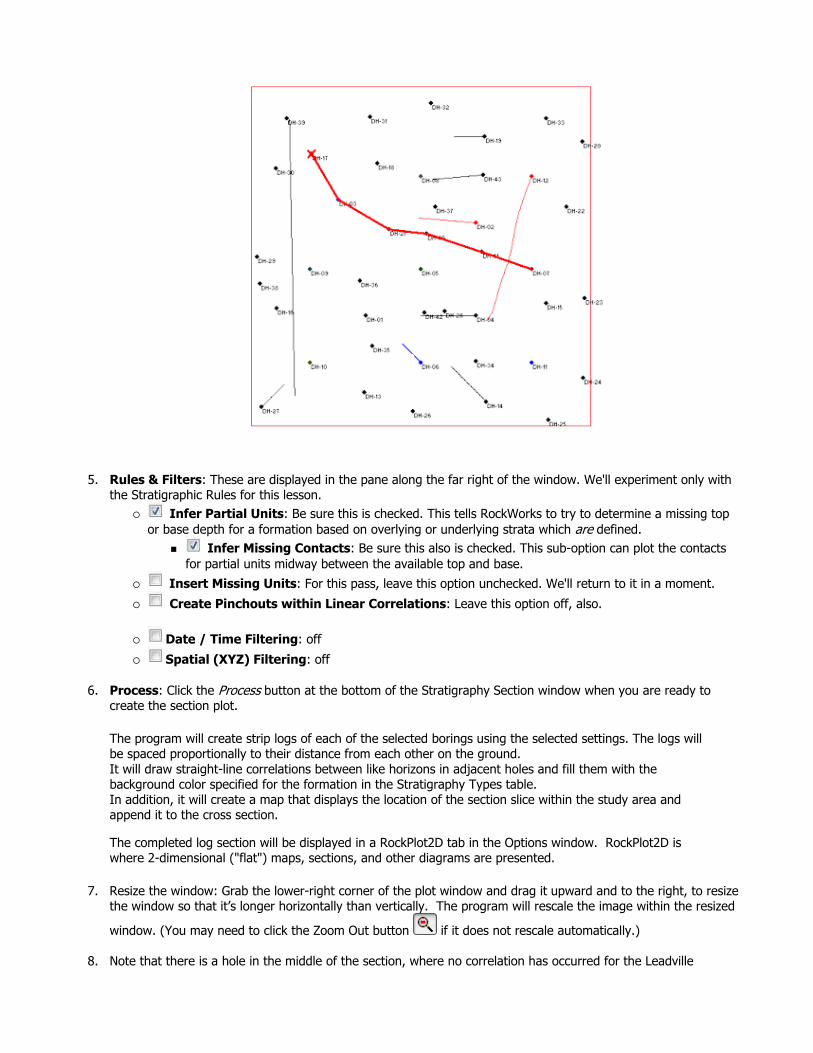
4. Next, pick the boreholes to display. Click on the Section Selection Map tab.
If you don't see the section trace pictured below, follow these steps; otherwise skip to step 5: Click on the Clear button at the top of the panel-picking window. The program remembers your cross section traces from session to session; this will clear any old traces from memory. Next, locate the hole titled "DH-17" (toward the upper-left) and click on it. It will be marked with a red "X". Locate hole "DH-03" southeast of "17" and click on it. A line will be drawn between the holes. Locate hole "DH-21" southeast of "03" and click on it.! If you make a mistake, click the Undo button to undo the last pick or the Clear button to clear the slate for starting over. Click on "DH-40," "DH-41," and "DH-07" continuing the cross section southeastward through the project area. You should see a trace like this:
5. Rules & Filters: These are displayed in the pane along the far right of the window. We'll experiment only with the Stratigraphic Rules for this lesson.
Infer Partial Units: Be sure this is checked. This tells RockWorks to try to determine a missing top or base depth for a formation based on overlying or underlying strata which are defined.
Infer Missing Contacts: Be sure this also is checked. This sub-option can plot the contacts for partial units midway between the available top and base.
Insert Missing Units: For this pass, leave this option unchecked. We'll return to it in a moment.
Create Pinchouts within Linear Correlations: Leave this option off, also.
Date / Time Filtering: off
Spatial (XYZ) Filtering: off
6. Process: Click the Process button at the bottom of the Stratigraphy Section window when you are ready to create the section plot.
The program will create strip logs of each of the selected borings using the selected settings. The logs will be spaced proportionally to their distance from each other on the ground.It will draw straight-line correlations between like horizons in adjacent holes and fill them with the background color specified for the formation in the Stratigraphy Types table.In addition, it will create a map that displays the location of the section slice within the study area and append it to the cross section.
The completed log section will be displayed in a RockPlot2D tab in the Options window. RockPlot2D is where 2-dimensional ("flat") maps, sections, and other diagrams are presented.
7. Resize the window: Grab the lower-right corner of the plot window and drag it upward and to the right, to resize the window so that it’s longer horizontally than vertically. The program will rescale the image within the resized
window. (You may need to click the Zoom Out button if it does not rescale automatically.)
8. Note that there is a hole in the middle of the section, where no correlation has occurred for the Leadville

Limestone (light blue) in DH-21.
If you move this window out of the way and click back into the Borehole Manager, click on DH-21, and click on the Stratigraphy button, note that the Leadville Ls. is missing from this hole.
9. Click back into the plot window, and now: Insert Missing Units: Insert a check in this option, in the Rules pane along the right. With this
turned on, the program will assume that formations which are missing entirely at a contact can be pinched out at that location. The program will insert them into proper sequence, with zero thickness, during the creation of the diagram. Note that this rule does not affect the data in the database, but instead adds the extra control when the data is processed for diagram generation. Click the Process button again to regenerate the diagram.
Now RockWorks has filled in the missing panel.
10. Adjust the Vertical Exaggeration: The VE notation, in the upper toolbar, is still shown at "1", meaning that the section's length (horizontal) and elevations (vertical) are being plotted at the same scale. In your own work, you may find that your distance and depth units aren’t so agreeable, and you’ll need to apply some stretch to your images to get a good look.
a. You can use either the Stretch button to fill the screen at whatever scales, or

b. You can adjust the vertical stretch specifically by clicking on the VE button (or choosing View | Vertical Exaggeration) and typing in a desired value.
11. Reposition the Stratigraphy Legend: In RockPlot2D you have the ability to edit the entities in the plot window.
a. Click on the Edit arrow in the upper-left corner. b. Click on the stratigraphy legend, on the right side of the diagram. When it is selected, you'll see handles
on each corner. c. Click on the legend and drag it to another location in the window. Release the mouse button when it is
positioned to your liking. d. To resize the legend, click and hold one of the corner handles and drag so that it is smaller or larger. e. If you like, you can double-click on the legend to see the options available in the Legend Attributes
window. There are settings that control the legend size, position, and appearance. Click OK to close the Attributes window.
12. Undock this cross-section into a stand-alone window by clicking the Undock button:
13. Save this image for later work in the ReportWorks program, where you can create a nice layout of the log profile and the section location map. With the section displayed in the new RockPlot window, choose File | Save, and type in the name: straight strat section and click Save. The program will save this image in its own ".Rw2D" file format.
Minimize this plot window for the time being, by clicking on the button in the upper-right corner.
14. Close the original cross-section plot window, by clicking in the Close button in the upper-right corner. You do not need to save the changes.
15. If you’d like to do the ReportWorks lesson at this time, click here.
16. Otherwise, continue on with the stratigraphy model lesson, below.
See also:
RockPlot2D tutorialHole to Hole Sections versus Profile Sections
Displaying Multiple Logs in a 2D Hole to Hole Section
Back to Stratigraphy menu | Next (3D Stratigraphic Model)
RockWare home page
Tutorial: Create a 3D Stratigraphy Model
Estimated time: 5 minutes.
In this lesson, you will create a 3D model of the project's stratigraphic surfaces.
Unlike a 3D lithology model (see that lesson) which uses a solid model to represent material types, the stratigraphic model represents multiple surface models, stacked on top of each other. The surfaces are interpolated from the stratigraphy contacts defined in the boreholes, using a process referred to as "gridding." (More.)
! You must be using RockWorks in Trial mode, or have a Level 4 or 5 license to run this modeling program.
1. Back at the Borehole Manager, with the Samples boreholes still displayed, click on the Stratigraphy menu and select the Model option.

2. Stratigraphy Types to be Included: Expand this heading and choose All Stratigraphic Units. (The other option offers a means of limiting the modeling to activated unts in the Types Table - handy for deep projects.)
3. Interpolate Surfaces: Be sure this is checked. This tells the program to interpolate surfaces for the units rather than use existing surfaces (e.g. from a previous run of this program).
Options: Click on this button (to the right) to access a window with a bunch of gridding options. Algorithms: These options determine the method that will be used to interpolate the surface models.
Triangulation: Choose this option for the modeling method. Interpolate Edge Points: Be sure this is checked.
! Note that if you choose a different gridding method, the options that are visible will change.
Grid Dimensions: Based on Output Dimensions: This should be the default setting. The surfaces will be
dimensioned as per the settings under the Output Dimensions. If you’d like to double-check these settings, you can click the Adjust/Examine Output Dimensions button to view the window you saw back in the Set Output Dimensions lesson.! In your own work, we recommend you choose this option so that the grid and solid model dimensions are consistent. However, the program does offer the option to vary the model dimensions, under the Variable Dimensions heading.
Confirm Dimensions: Uncheck this (though in your own work, this is a handy way to double-check the model extents and node spacing).
Additional Options: Set these options. Decluster: On
Logarithmic: Off
High Fidelity: Off
Polyenhanced: Off Smooth Grid: On (Default size and Iterations = 1)
Densify: Off
Maximum Distance: Off
Z = Color: Off
Faulted: Off Click the OK button to accept these gridding settings.
Other modeling options - expand the Interpolate Surfaces heading to access these settings: Onlap: On. This assures that lower formations have "priority" and upper layers cannot fall
below or interfere with lower layers.
Constrain Model Based on Ground Surface: Off (This allows you to filter the uppermost unit using a ground surface model.)
Polygon Filter: Off
Baseplate: Uncheck this.
4. Save Numeric Model: On. This tells the program to build a solid model file behind the scenes, representing the stacked stratigraphic surfaces. This solid won't be used at this time, but we'll use it a bit later for volume computation. Expand the Save Model heading.
Model Name: Click to the right and type in: stratigraphy and click the Save button. The ".RwMod" file name extension will be added automatically.More on stratigraphic models.
5. Diagram Options: Expand this heading to establish the diagram options.
Explode: Uncheck this. (It's used to insert space between the units when displayed in 3D.)
Hide Thin Zones: Uncheck this. Plot Logs: Yes. The defaults from the first lesson should still be established. Feel free to click on the
3D Striplog Designer tab to the right to double-check the 3D log setup if you wish.
Reference Cage: Unchecked. Include Stratigraphy Legend: Check this.
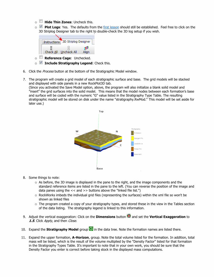
6. Click the Process button at the bottom of the Stratigraphic Model window.
7. The program will create a grid model of each stratigraphic surface and base. The grid models will be stacked and displayed with side panels in a new RockPlot3D tab.(Since you activated the Save Model option, above, the program will also initialize a blank solid model and "insert" the grid surfaces into the solid model. This means that the model nodes between each formation’s base and surface will be coded with the numeric "G" value listed in the Stratigraphy Type Table. The resulting stratigraphic model will be stored on disk under the name "stratigraphy.RwMod." This model will be set aside for later use.)
8. Some things to note: As before, the 3D image is displayed in the pane to the right, and the image components and the standard reference items are listed in the pane to the left. (You can reverse the position of the image and data panes using the << and >> buttons above the "linked file list.") RockWorks imbeds the individual grid files (representing the surfaces) within the xml file so won't be shown as linked files The program created a copy of your stratigraphy types, and stored these in the view in the Tables section of the data listing. The stratigraphy legend is linked to this information.
9. Adjust the vertical exaggeration: Click on the Dimensions button and set the Vertical Exaggeration to 1.5. Click Apply, and then Close.
10. Expand the Stratigraphy Model group in the data tree. Note the formation names are listed there.
11. Expand the upper formation, A-Horizon, group. Note the total volume listed for the formation. In addition, total mass will be listed, which is the result of the volume multiplied by the "Density Factor" listed for that formation in the Stratigraphy Types Table. It's important to note that in your own work, you should be sure that the Density Factor you enter is correct before taking stock in the displayed mass computations.

12. Remove the check-mark from the next formation, Spergen Fm, and see how that entire formation will be removed from the image view. Remove the check-mark from the next formation, Leadville Fm, as well, and it will disappear.
13. Expand the next formation, Potosi Fm, in the data tree, and expand its Top group. Double-click on the formation top’s Elevation Grid.
14. Click in the Color Scheme drop-down list, and choose the Continuous option. Click Apply to see how the upper surface of the formation is now displayed in color.
15. Click Close to close the Grid Options window.
16. Save this image by choosing File | Save As. Enter the name: strat model and click the Save button. The file "strat model.Rw3D" will be stored in your project folder.
17. Other things to try: Double-click on the Stratigraphy Model group icon - the parent of all of the formation groups - and set the Opacity setting for the whole image to 70 and click Apply. Change the font size or style in the stratigraphy legend by expanding the Legends heading, double-clicking on the Stratigraphy legend item, clicking on the Font button, and selecting a different font size or style.
Stratigraphy Models, Gridding Reference
Back to Stratigraphy menu | Next (interpolated cross section)
RockWare home page
Tutorial: Create a Modeled Stratigraphic Cross Section
Estimated time: 3 minutes.
In this lesson, you will use the stratigraphic surface models created in the previous lesson, and create a multi-panel cross section. This will be similar to the cross section you created previously in this lesson set, except that the correlation panels are based on the interpolated grid models rather than straight-line correlations.
! The instructions below are written with the assumption that you have completed the Cross Section lesson and the Stratigraphy Model lesson.
1. Click on the Stratigraphy menu and choose Section.
2. Correlation Options: Expand this heading. Fill Background: Check this box. The panels will include the background colors defined for the units
in the Stratigraphy Type Table. Plot Patterns: Uncheck this. By displaying only colors on the panels themselves, this makes it easier
for the patterns in the striplogs to stand out. Plot Outlines: Uncheck this.
3. Interpolate Surfaces: Uncheck this box since you already modeled the surfaces in the previous lesson.! This is really important - if you have a good stratigraphic model created, you don't need to keep reinterpolating the surfaces just to create a new type of diagram to display.
4. Other settings: These should still be default from previous lessons.
Smoothing Passes: This can be set to 1. Stratigraphy Legend: Yes. Plot Logs: Yes. (The current 2D Striplog Designer settings should be fine, from previous lessons.)
Plot Surface Profile: Uncheck this.
Show Fault(s): Uncheck this. Perimeter Annotation Options: As before.
Create Separate Location Map: Yes
Clip (Vertically Truncate) Diagram: Uncheck this. In your own work, this can be used to display an elevation subset of the entire model. Section Selection Map: We'll use the same section trace from the previous lesson.
5. Click the Process button when you are ready to continue.
The program will read the existing surface models and extract panels along the indicated cross-section trace. It will build them into a continuous cross section diagram, with the indicated perimeter annotation. The stratigraphy logs will be appended to the section diagram. The completed diagram will be displayed in a new RockPlot2D tab.
6. Resize the section window so that it is longer than it is tall and laying along the bottom of your screen. As you resize the window, the section will be resized within it, accordingly. If, by chance, it is not, click the small Zoom-
Out button to replot the section in the new window space.
7. Bring up the previously-saved straight section by hovering over the RockWorks icon on the Windows taskbar, and clicking on the RockPlot2D - Straight Strat Section window.
Arrange the windows so that you can compare their appearance. The benefits of modeled sections are that they look smoother and better represent the stratigraphic data near as well as along the section cut. Straight sections are helpful by displaying the data as entered. They can highlight data errors as well as formation discontinuities.
We often create straight sections first to determine boreholes where data should be checked and missing formations dealt with – whether they are left blank or are entered with a thickness of zero will have different effects. You can refer to the "missing formations" topic in the Help messages for details (link below).
8. Save the modeled section using the File| Save As menu command. Type in the name: strat mod sectionand click the Save button.
Creating Interpolated Stratigraphic Sections, Missing Formations
Back to Stratigraphy menu | Next (2D structure maps)
RockWare home page
Tutorial: Create a 2D Stratigraphic Structure Map
Estimated time: 5 minutes.
Let's move from profile-type views to plan-views of the stratigraphic units. First we’ll create a 2D or "flat" contour map of the surface of one of the stratigraphic units. In the process of building the contour map, the program will create a grid model of the surface elevations, just like the ones created for the stratigraphic model in a previous lesson.
! You must be using RockWorks in Trial mode, or have a Level 4 or 5 license to run this modeling program.
1. Click on the Stratigraphy menu at the top of the program window, and select Structural Elevations | 2-Dimensional.
2. Stratigraphic Unit: Click here to select the unit to be modeled. In the displayed window, which lists the formation names in the Stratigraphy Types Table, click on the item Leadville Ls.Expand the Stratigraphic Unit heading.
Superface (Top): Click in this button to specify the model is to represent the top of the formation.
3. Establish gridding settings: Grid (Output): Click to the right and type in the following name for the surface’s grid model: leadvilleGridding Options: Click here if you wish, to review the gridding settings used in the previous lessons. We'll use the same settings here.
4. Diagram Options: Expand this heading to establish the diagram options.
Background Image: Uncheck this. Contour Lines: Check this.
Click the Options button (to the right). For this tutorial the defaults settings should be fine. (Intervals = Regular , Confirm Intervals= off; Label Contours = on; all Filters and Faults settings off.) Click OK to close this window.
Colored Intervals: Check this option. Click on the Options button (to the right) to see all of the color-contouring options. The defaults should be fine. You can click on the color bar to view some of the other options. Click OK to close this window.
Fault Polylines: Uncheck this.
Labeled cells: Uncheck this. Borehole Locations: Check this. Expand this heading.
Click on the Borehole Symbol & Label Options button. Be sure the following items are turned on:
Symbols: This should be checked, so that the borehole locations will be represented with map symbols shown on each well’s Location tab.
Log Traces: You can turn these on. Borehole IDs: This should be checked, so that the map symbols will show the well
name. Stratigraphy Data: Check this box, so that we can label the Leadville elevations.
Stratigraphic Unit: Click this to select the Leadville Ls. formation name. Superface Elevation: Check this option.
Remove all other checks from the stratigraphy label options. Label Options: Click here.
Auto-Offset: check this box. The other defaults should be fine.
Click OK to accept these changes and close the symbol & label options window. Border: Check this. The defaults should be fine.
5. Click the Process button to continue.
The program will read the well location and downhole survey information from the Borehole Manager tabs
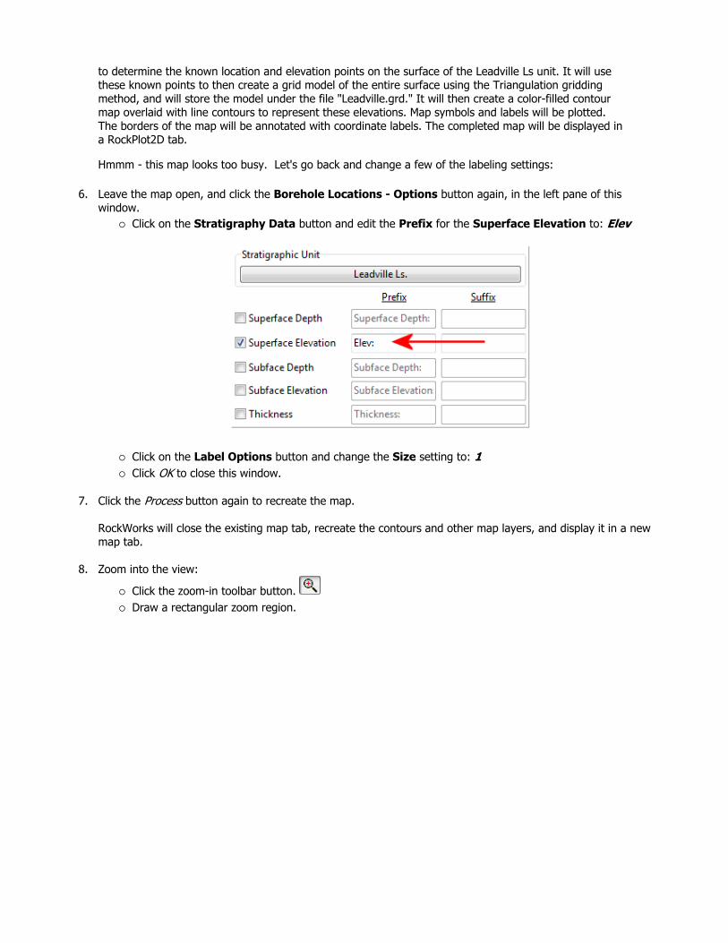
to determine the known location and elevation points on the surface of the Leadville Ls unit. It will use these known points to then create a grid model of the entire surface using the Triangulation gridding method, and will store the model under the file "Leadville.grd." It will then create a color-filled contour map overlaid with line contours to represent these elevations. Map symbols and labels will be plotted. The borders of the map will be annotated with coordinate labels. The completed map will be displayed in a RockPlot2D tab.
Hmmm - this map looks too busy. Let's go back and change a few of the labeling settings:
6. Leave the map open, and click the Borehole Locations - Options button again, in the left pane of this window.
Click on the Stratigraphy Data button and edit the Prefix for the Superface Elevation to: Elev
Click on the Label Options button and change the Size setting to: 1Click OK to close this window.
7. Click the Process button again to recreate the map.
RockWorks will close the existing map tab, recreate the contours and other map layers, and display it in a new map tab.
8. Zoom into the view:
Click the zoom-in toolbar button. Draw a rectangular zoom region.

9. Edit the contour line's label.
Click the Edit button in the toolbar. Click on the labeled contour line. The program will display it with handles at each polyline inflection point. Right-click and choose Properties. Change the Font Color to red. Click Apply and Close.The program will display the font label in red.
10. Zoom back out: click the Zoom-Out button.
11. Close this window by clicking on the Windows close button ("X") in the upper-right corner. You can answer "no" to the do-you-want-to-save prompt.
Creating 2D Stratigraphic Structure Maps
Back to Stratigraphy menu | Next (Volume report)
RockWare home page
Tutorial: Run a Stratigraphy Volume Report
Estimated time: 1 minute.
Finally, let’s run a quick volume report for the stratigraphic layers. The computed totals will be displayed in a data tab.
We assume that you have gone through the Stratigraphy Model lesson, and in that lesson created a solid model of the layers, saved in a file "stratigraphy.RwMod" for volume computation.
1. At the Borehole Manager, choose the Stratigraphy|Volumetrics (Based on Solid Model) option.

2. Stratigraphy Model: Click here to browse for your model, named stratigraphy.RwMod.
3. Output Options: Nodes: Uncheck this. Volume: Check this.
Mass: Uncheck this. Percent: Check this.
4. Intervals: Every Layer.
5. Decimals: This can be set to 0.
6. Click Process to continue.
The program will create a data tab where it will display the total volume for each defined formation at every layer in the solid model. It will also display percent of that type for that layer. If you scroll down to the bottom of the data listing, the overall totals will be displayed.
7. To save this datasheet, click on the File | Save option at the top of the window, and type in the name: stratigraphy volumes and click Save. The program will append the ".RwDat" file name extension automatically. These are files that you can open into the RockWorks Utilities datasheet.
8. If the RockPlot3D window containing your stratigraphic model is still open, you can compare the volume notations there with those in the datasheet. They'll likely be different because they represent different methods of computing volumes. The surface-based volumes, as displayed in the RockPlot3D window, are probably the more accurate since they are slightly less dependent on the resolution of the models as is the solid-based volume report.
9. If you have a moment, you can return to the main menu and run the Stratigraphy | Volumetrics (Based on Surface Models) option, to compare the calculations. Generally, the volumes computed for the surface-based model will be more accurate than the volumes computed for the solid-based model.
This is the end of the tutorial for stratigraphy data. The next section contains lessons for downhole interval-sampled data.
Computing Stratigraphy Volumes
Back to Stratigraphy menu | Next (I-Data Diagrams)
RockWare home page
Tutorial: Create I-Data Models and Diagrams

This section of the Borehole Manager tutorial contains lessons for creating diagrams to illustrate downhole data that’s entered into the project’s I-Data (Intervals) tables. I-Data simply refers to downhole samples that are measured over depth intervals rather than at depth points. This is commonly used for geochemical and geotechnical data.
If you have already done the lithology or stratigraphy lessons, some of these procedures will be very much the same. However, rather than illustrating rock types only in logs, the downhole interval data will be illustrated as bargraphs in the logs. A solid model will be created to illustrate the isosurface, multi-panel section, and fence diagram.
(See also time-based interval data lessons in the T-Data section.)
Pick a lesson by clicking on its arrow. We recommend going through these lessons in the order listed.
If this is the first lesson set you’ve done, please be sure you’ve (1) restored the program defaults, (2) opened a project folder, and (3) set the project dimensions.
Tutorial LessonRequired licensing level
Look at the Interval Data layout. See how the data columns and values are defined, how to edit the data as a spreadsheet, how to generate a frequency histogram of values, and how to query based on I-Data values.
Trial orLevel 4
Display I-Data logs in 3D. This offers a quick, overall view of the Benzene Soil data as entered, across the project.
Trial orLevel 3
Display I-Data logs in a 2D cross section. This shows the Benzene Soil measurements for selected boreholes in a multi-log cross section diagram.
Trial orLevel 3
Create a 3D I-Data isosurface diagram. Here you will interpolate the log data into a continuous solid model and display it as an isosurface.
Trial orLevel 4
Create an interpolated I-Data cross section. Using the interpolated model, you'll display connected slices in a cross section diagram.
Trial orLevel 4
Create an I-Data fence diagram. Using the interpolated model, you'll display multiple panels in a 3D fence diagram.
Trial orLevel 4

Back to main menu
RockWare home page
Tutorial: View the Interval Data Layout
Estimated time: 5 minutes.
In this lesson, you will look at how downhole "Interval" data is entered, how the columns are defined, how to edit the data as a "datasheet", how to generate a frequency histogram of the values, and how to do a simple query.
1. Be sure the "Samples" folder is still the current project folder (see Open a Project for information).
2. In the borehole file listing along the left side of the Borehole Manager, click on the borehole named "DH-02" to make it active.
3. Click on the I-Data button, so that the I-Data (Interval-Data) table is displayed.
! Note how each row contains a top and bottom depth, and multiple columns of measurements. These values can represent mineral assays, pollutant concentrations, percent gravel, or any quantitative measurement taken over a depth interval. If a component has no measurement for that interval, it can be left blank.
4. Click on the borehole "DH-04" in the list to the left, and you’ll see the information listed in its I-Data table.

There's no limit to the number of components for which you can enter measurements. Let's take a look.
5. Look at the project's I-Data Types: a. Click on the I-Data Types button at the top of the I-Data listing. The program will display the current I-
Data setup.
This defines for each component type its name (required) and its min and max values. You can also enter comments regarding units and descriptive notes. The Order column determines the left-to-right order of the columns in the display. The Visible check-box allows you to turn on/off the column display.
In your own work you can add components to the I-Data table (and columns to the Borehole Manager display) by clicking in the last shown row, pressing the down-arrow key, and defining these fields for the new measurement type.
b. Click on the Close button to close the window.
! You can also access the Interval (I-Data) Columns window via the Project Manager pane: Expand the Project Tables | Types Tables heading, and double-click on the I-Data Types item.
6. Edit as Datasheet: Note that even though the data displayed in the I-Data tab looks like a spreadsheet, it is not. It's actually a rather complicated merging of many records stored in the Borehole Manager's I-Data and I-Data Type tables. Because of this, you cannot select a block of cells like you can within a spreadsheet-type display, or copy/paste blocks of cells.There is, however, a nifty tool in the Edit menu that makes editing this data quite easy.
a. Click on the Datasheet button at the top of the I-Data listing for the current borehole. (Or select the Edit | Edit Data as Datasheet menu option.)
b. The program will load the contents of the I-Data table, for the current borehole, into a row-and-column datasheet editor window. Here you can select blocks of cells, copy and paste from other applications, etc.
c. Close this window by clicking the X button, and respond Yes to the Cancel-all-changes prompt (if it is displayed).
7. Generate a Frequency Histogram of Benzene measurements, which will give us a quick look at the distribution of the data:
a. Back at the Borehole Manager window, click on the I-Data menu at the top of the program window, and choose the Histogram option.
b. Enter the following: I-Data Track: Click here and choose Benzene Soil. Primary Title: Click here and type in: Benzene Soil StatsSecondary Title: Click here and delete all text.

The remaining defaults should be fine. c. Click the Process button at the bottom of the window to continue.
The program will read through all of the Benzene Soil measurements for all boreholes, compute the mean and standard deviation, and generate a frequency histogram plot. This diagram will be displayed in a RockPlot2D tab in the options window.
Let's say we're interested in finding those boreholes with the anomalous high readings. We can use the Query tools, next.
e. Click the Windows Close button to close the I-Data Histogram window. You can click No at the save-file prompt.
8. Query the Data: Let's use the basic query tool in RockWorks to enable only those boreholes that have Benzene Soil values > 75 ppm.
a. Choose the View | Filter Boreholes option. You'll see a window where there are number of data filtering options.
b. Surface Region: Uncheck this. We won't be filtering by borehole location. c. Interval Data Values: Check this box in the column along the left.
i. I-Data name: Click the down-arrow button and choose the Benzene Soil option. ii. From: In this prompt, enter 75 iii. To: In this prompt, enter 999 iv. Apply: Click the Apply button at the bottom of the window. You'll see a preview to the right,
displaying in red those boreholes that contain Benzene Soil measurements ranging from 75 to 999, and all others in gray.
d. All other Select By... options should be left un-checked. e. Click OK.
Back at the Borehole Manager, you'll most of the boreholes are now inactive - they are no longer shown with check-marks. Disabled boreholes will not be displayed in maps or log displays, and their data will not be included in any modeling.
! The View | Filter Boreholes option uses an "AND" type of query, in which each of the boreholes for which every criterion is true will be enabled and the remaining boreholes will be disabled. The View | Select Boreholes option is more complex, allowing successive filters to be applied, and the enabling/disabling will apply only to the boreholes meeting the filter parameters, and no others. So, while the Filter Boreholes tool works as an AND filter, the Select Boreholes tool can function as an AND or OR filter.
Entering I-Data
Back to I-Data menu | Next (3D logs)

RockWare home page
Tutorial: Display I-Data Logs in 3D
Estimated time: 4 minutes.
In this lesson, you will get a quick view of one I-Data component (Benzene) as entered for the project’s boreholes, by generating 3D benzene logs for the currently-enabled boreholes.
1. Enable all boreholes: Select the Edit | Enable All Boreholes. (Or click the button on the toolbar to the left of the borehole names.)
2. To create the 3D logs, click on the Striplogs menu, and then click on 3-Dimensional | Multiple Logs.
This window has several sections:The left side is where general diagram settings are established.The 3D Striplog Designer tab is where you establish the log-specific settings.
3. Establish the general diagram settings in the left pane. Group Title: This can be left at: Logs
Clip: Uncheck this. Reference Cage: Check this.
Include Lithology Legend: Uncheck this.
Include Stratigraphy Legend: Uncheck this.
Include Well Construction Legend: Uncheck this.
Include Aquifer Legend: Uncheck this.
4. Click on the 3D Striplog Designer tab.
The left pane is where you choose what type of data is to be displayed in the logs (the Visible Items). The upper-right pane is where you see a plan-view Preview of the active log items. You can drag the items to adjust their relative placement. The lower-right pane displays specific Options for the Visible Item that you click on.
Choose the items you want to see in the logs by inserting a check-mark in the following items in the Visible Items section of the window:
Title: The drill hole name will plot above the logs. Axis: The logs' axes will be shown with a solid line. I-Data #1: The logs will contain a column illustrating interval-data values. You can include up to 4
different I-Data "tracks"; we'll display only one in this lesson.When you insert a check in the I-Data #1 item (under Visible Items), you'll see a purple circle displayed in the plan-view Preview pane.
Track: At the top of the Options pane, click on the Track heading and choose Benzene Soil as the data to be represented in the logs. Expand the Track heading to access the data filter options.

Filter Based on G Values: Be sure this is left un-checked. In your own work this can be used to display only high or low values in your logs.
Resample at Regularly-Spaced Intervals: Be sure this is also left un-checked. In your own work, these settings can be used to thin the number of downhole measurements displayed (for densely sampled drillholes) or to include zero-value "bogus" points to add control to sparsely-sampled holes.
Column Title: This should be blank. If text is displayed for this prompt, click on this heading and delete the text.
Plot Interval Labels: Leave this unchecked (it's used to plot value labels down the log). Offset Direction: This should reflect the current offset, in azimuth degrees, from the axis of the log. It can be left at zero. Offset Distance: Adjust the placement of the column relative to the axis of the log by dragging the circle in the Preview pane. Be sure the I-Data circle is on the center of the log axis.! You can simply type 0.0 into the Offset Distance prompt, if you prefer. Column Radius: You can adjust the size of the column by dragging on one of the corner handles. Note the Column Radius setting in the lower-right Options pane. As you resize the circle, the Radius setting will be updated. Drag the I-Data #1 circle until the Column Radius is about 2.0.! You can simply type 2.0 into the Column Radius prompt, if you prefer. Scaling: Expand this heading and select Automatic. Fill Style: Expand this Options heading, and choose Variable. This will color-code the logs based on Benzene Soil values. Shape: Expand this Options heading, and choose Oblates.
None of the other Visible Items should be checked. Here's a summary of these settings.

5. Click the Process button at the bottom of the Multiple Log 3D Plotting window to proceed.
The program will create a log for each enabled borehole, including well name at the top, and color-coded Benzene Soil disks displayed down the log. They will be displayed in a new RockPlot3D tab.
The image is displayed in the pane to the right, and the image components as well as the standard reference items are listed in the pane to the left. The expandable/collapsible list on the left is called the "data tree."
6. Adjust the Reference items: Turn off the World Outline (if it’s on), by clearing its check-box in the upper portion of the left-hand listing. (Since there’s a reference grid in this image, the world outline is redundant.) Be sure the Axes and Labels are both turned on.
7. Set the view to a fixed viewpoint: Click on the View menu and choose Compass Points | East.
8. Since the logs will appear lined up behind each other, click and hold on the south-north midline and drag slightly to the right to rotate around the vertical axis so that you can see the background logs. Try to keep the image straight up and down. Release the mouse button. Next, click and hold on the top-base axis line and drag slightly downward to rotate the image around the horizontal axis. This will give the display a 3-dimensional view.! If you lose track of where you are in the 3D display, you can always return to the View menu to choose a pre-set viewpoint, such as Compass Points | East, or Above | Southwest (the default view).
9. Zoom into the logs along the left side of the display: Click the Zoom button in the toolbar, and click and drag in the image as shown below to draw an enlargement rectangle.
Note that you can also enlarge / reduce 3D views using the Percent drop-down at the top of the window.
Another tip: Hide the left-hand menu, filling the window with the graphic display, using the small "-" button in the divider.
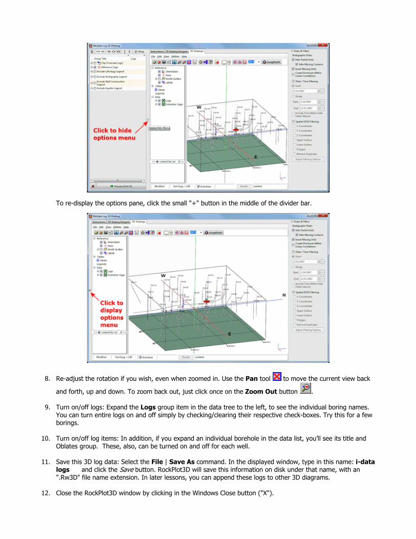
To re-display the options pane, click the small "+" button in the middle of the divider bar.
8. Re-adjust the rotation if you wish, even when zoomed in. Use the Pan tool to move the current view back
and forth, up and down. To zoom back out, just click once on the Zoom Out button .
9. Turn on/off logs: Expand the Logs group item in the data tree to the left, to see the individual boring names. You can turn entire logs on and off simply by checking/clearing their respective check-boxes. Try this for a few borings.
10. Turn on/off log items: In addition, if you expand an individual borehole in the data list, you’ll see its title and Oblates group. These, also, can be turned on and off for each well.
11. Save this 3D log data: Select the File | Save As command. In the displayed window, type in this name: i-data logs and click the Save button. RockPlot3D will save this information on disk under that name, with an ".Rw3D" file name extension. In later lessons, you can append these logs to other 3D diagrams.
12. Close the RockPlot3D window by clicking in the Windows Close button ("X").

3D Logs
Back to I-Data menu | Next (2D log section)
RockWare home page
Tutorial: Display Multiple Bargraph Logs in a 2D Cross-Section
Estimated time: 6 minutes.
In this lesson, you will be creating an image representing the benzene I-Data measurements in multiple logs in the Samples project, selected along a multi-log cross section trace. You will also add simple correlations panels.
1. Be sure all of the boreholes in the project are enabled by clicking on the Edit|Enable All Boreholes menu
option or toolbar button.
2. Click on the Striplogs menu, and then click on 2-Dimensional | Section. (What's the difference between "profiles" and "sections"? Click here.)
3. Establish the section options:These are found in the left pane of the Hole-to-Hole Log Section window. Plot Striplogs: Check this.
Borehole Spacing: Expand this heading if necessary and be sure that this is set to Distance between Collar Locations. (In your own work, the Uniform Distance option can be handy if you have lots of clustered wells.)
Plot Correlations: Leave this un-checked for now (we'll experiment with this momentarily).
Hang Section on Datum: Uncheck this.
or Plot Surface Profile: If you completed the borehole map section of the tutorial (jump back), insert a check in the Plot Surface Profile option. This is used to display a selected surface in the cross section plot. If you DID NOT complete that lesson, leave this un-checked.
Grid Model: Click here and select the GRD file representing the ground surface, named surface.RwGrd and click the Open button. Line Type: Click here to set the line style to red, medium thickness. Smoothing can be set to 1.
Show Faults: Uncheck this.
Perimeter Annotation Options: These options determine text and lines that will plot around the perimeter of the profile. Click on the Options button to view the settings; the factory defaults should be fine. See Restore Default Settings if you need more information about setting the factory defaults. Click OK to close this window.! In your own work the Intended Vertical Exaggeration Factor can be very helpful for good diagram proportions if you have a large, flat study area and will stretch your cross sections for readability.

Create Location Map: Check this item. This will create a small map that shows the location of the profile "cut" in the study area. Expand this heading to change:
Append Map to Profiles + Sections: Check this option. Expand this heading and be sure the Size setting is set to Medium.In your own work, don't choose Append if you will be applying vertical exaggeration to your section... the map will stretch as well!
Display Map as Separate Diagram: Uncheck this option.
Legends: Click on the Options button.
Aquifers: Uncheck this item.
Lithology: Uncheck this.
Stratigraphy: Uncheck.
Well Construction: Uncheck. Click OK to close the Legend Options window.
Clip (Vertically Truncate) Diagram: Uncheck this.
4. Establish the striplog options: Now you need to set up how the logs within the cross section will look. Click on the 2D Striplog Designer tab, to the right.
The program will display the 2D log designer window. This window has three main sections: The left pane is where you choose what type of data is to be displayed in the logs (the Visible Items). The upper-right pane is where you see a Preview of the active log items. You can drag the items to adjust their relative placement. The lower-right pane displays specific Options for the Visible Item that you click on.
a. Choose the items you want to see in the logs by inserting a check-mark in the following items in the Visible Items section of the window:
Title: The drill hole name will plot above the logs. Depths: The logs will be labeled with depth tick marks and labels. I-Data #1: The logs will contain a column illustrating I-Data values as a bargraph down the log.
Note that you can activate up to 4 I-Data columns. None of the other options, including Text, should be checked.
b. Adjust the arrangement of the visible log items: You should see four items in the upper Preview pane: title, depth bar, log axis, and I-data column.
Practice clicking on an item, holding down the mouse button, and dragging it to the left or right in the preview.
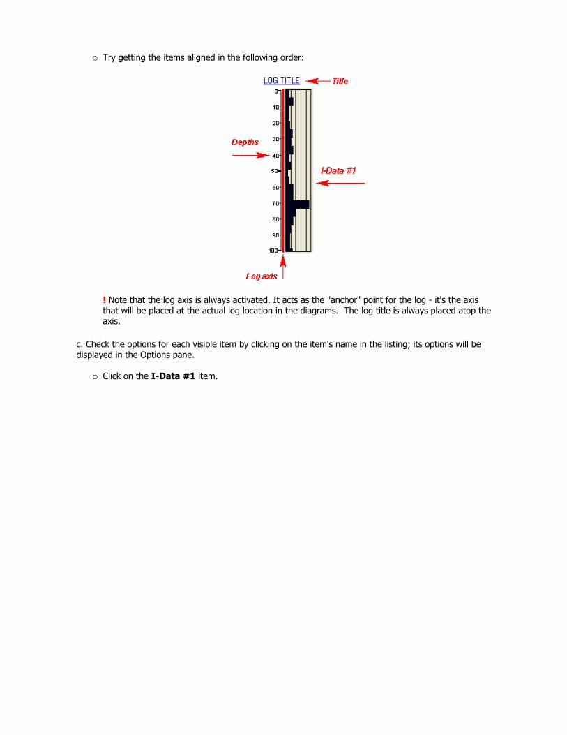
Try getting the items aligned in the following order:
! Note that the log axis is always activated. It acts as the "anchor" point for the log - it's the axis that will be placed at the actual log location in the diagrams. The log title is always placed atop the axis.
c. Check the options for each visible item by clicking on the item's name in the listing; its options will be displayed in the Options pane.
Click on the I-Data #1 item.

Track: Click to the right and choose Benzene Soil as the data to be displayed in the logs.
Background Subdivisions: Uncheck this item. Width: Click on this item, above the Column Title, and set the Width to 2. ! All log item sizes are expressed as a percent of the dimensions of the project, so the width of these logs will be about 1% of the project dimensions. Fill Style: Scroll down to find this heading in the Options pane.
Monochrome: Choose this Fill Style option and set the color to blue. Direction: Look for this heading in the Options pane.
Left-to-Right: Choose this option.
5. Next, pick the boreholes to display. Click on the Section Selection Map tab.
If you don't see the section trace pictured below, follow these steps; otherwise jump to #6 below. Click on the Clear button at the top of the panel-picking window. The program remembers your cross section traces from session to session; this will clear any old traces from memory. Next, locate the hole titled "DH-17" (toward the upper-left) and click on it. It will be marked with a red

"X". Locate hole "DH-03" southeast of "17" and click on it. A line will be drawn between the holes. Locate hole "DH-21" southeast of "03" and click on it.! If you make a mistake, click the Undo button to undo the last pick or the Clear button to clear the slate for starting over. Click on "DH-40," "DH-41," and "DH-07" continuing the cross section southeastward through the project area. You should see a trace like this:
6. Click the Process button at the bottom of the window when you are ready to create the log section plot.
The program will create strip logs of each of the selected borings using the selected settings. The logs will be spaced proportionally to their distance from each other on the ground.
In addition, it will create a map that displays the location of the section slice within the study area. The completed log section + map will be displayed in a RockPlot2D tab, where 2-dimensional ("flat") maps and other diagrams are presented.
7. Let's return briefly to the options on the left side of the screen, to recreate the section with quick correlation panels. These are not extracted from a 3D block model (as you'll do in a later lesson) but instead they're interpolated from the two endpoint logs only. This type of "quick-section" will not take into account any other neighboring holes, but they can give you a quick look at the data.
Plot Correlations: Locate this setting in the options along the left side of the window. Check this box, and expand this heading.
I-Data: Click in this button. Expand the heading. I-Data Track: Click to the right to choose Benzene Soil.
I-Data & P-Data Section Options: Expand this heading.
Contour lines: Be sure this is not checked. Colored Intervals: Be sure this is checked.
8. Click Process at the bottom of the window. RockWorks will regenerate the section, now with the correlation panels.
9. Hide the options pane to enlarge the section window: Click on the small "-" button in the divider bar to the left of
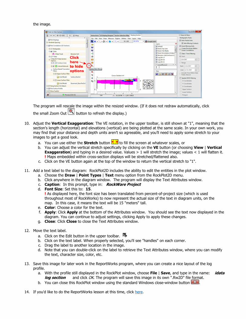
the image.
The program will rescale the image within the resized window. (If it does not redraw automatically, click
the small Zoom Out button to refresh the display.)
10. Adjust the Vertical Exaggeration: The VE notation, in the upper toolbar, is still shown at "1", meaning that the section's length (horizontal) and elevations (vertical) are being plotted at the same scale. In your own work, you may find that your distance and depth units aren’t so agreeable, and you’ll need to apply some stretch to your images to get a good look.
a. You can use either the Stretch button to fill the screen at whatever scales, or b. You can adjust the vertical stretch specifically by clicking on the VE button (or choosing View | Vertical
Exaggeration) and typing in a desired value. Values > 1 will stretch the image; values < 1 will flatten it.! Maps embedded within cross-section displays will be stretched/flattened also.
c. Click on the VE button again at the top of the window to return the vertical stretch to "1".
11. Add a text label to the diagram: RockPlot2D includes the ability to edit the entities in the plot window. a. Choose the Draw | Point Types | Text menu option from the RockPlot2D menu. b. Click anywhere in the diagram window. The program will display the Text Attributes window. c. Caption: In this prompt, type in: RockWare Projectd. Font Size: Set this to: 15.
! As displayed here, the font size has been translated from percent-of-project size (which is used throughout most of RockWorks) to now represent the actual size of the text in diagram units, on the map. In this case, it means the text will be 15 "meters" tall.
e. Color: Choose a color for the text. f. Apply: Click Apply at the bottom of the Attributes window. You should see the text now displayed in the
diagram. You can continue to adjust settings, clicking Apply to apply these changes. g. Close: Click Close to close the Text Attributes window.
12. Move the text label. a. Click on the Edit button in the upper toolbar. b. Click on the text label. When properly selected, you'll see "handles" on each corner. c. Drag the label to another location in the image. d. Note that you can double-click on the label to retrieve the Text Attributes window, where you can modify
the text, character size, color, etc.
13. Save this image for later work in the ReportWorks program, where you can create a nice layout of the log profile.
a. With the profile still displayed in the RockPlot window, choose File | Save, and type in the name: idata log section and click OK. The program will save this image in its own ".Rw2D" file format.
b. You can close this RockPlot window using the standard Windows close-window button .
14. If you’d like to do the ReportWorks lesson at this time, click here.

15. Otherwise, continue on with the I-Data diagram lessons, below.
See also: RockPlot2D tutorial
Displaying Multiple Logs in a 2D Hole to Hole Section
Back to I-Data menu | Next (model & isosurface)
RockWare home page
Tutorial: Create an I-Data Model and Isosurface Diagram
Estimated time: 4 minutes.
Now we will jump from the Striplogs menu, where we plotted observed data in log diagrams, to the I-Data menu, where the downhole quantitative data will be interpolated into a continuous model.
In this lesson, you will create a solid model and 3-dimensional isosurface diagram of the project's Benzene Soil measurements. The program will load the recorded borehole data, that you viewed in logs and log sections already, and extrapolate the benzene values throughout the project. This modeling process basically "fills in the blanks" between the logs. RockWorks offers several modeling algorithm to do this extrapolation.
! You must be using RockWorks in Trial mode, or have a Level 4 or 5 license to run this modeling program.
Before continuing, be sure you have opened the sample project, established the output dimensions and created 3D logs, as discussed in earlier lessons.
1. Back at the Borehole Manager, click on the I-Data menu and select the Model option.
2. Establish the modeling settings: Create New Model: Click in this button, and expand this item to define the input data and modeling
settings.
I-Data Track: Click here to select from the pop-up list the column titled Benzene Soil. Expand this heading and be sure that none of the data filters are turned on.
Solid Model Name: Click to the right of this label and type in: benzene soilThis will be the name assigned to the solid model to be created, with an ".RwMod" file name extension.
Solid Modeling Options: Click the Options button to the right, to access the various modeling settings. Algorithms: These options determine the method that will be used to interpolate the I-Data model. If you’ve restored the program defaults, the IDW Anisotropic method (which represents Inverse-Distance, Anisotropic) should be selected. This will be fine; you can click on that tab to read additional information.! Note that if you choose a different modeling method, the options that are visible will change. Additional Options - Turn the following items on/off. Note that you can click on any of these tabs to read more information.
Dimensions: These define the extents of the output model. Based on Output Dimensions: Be sure this option is checked.
Confirm Model Dimensions item can be left unchecked (though in your own work, this is a handy way to double-check the model extents and node spacing).
Decluster: Checked.
Add Points: unchecked.
Cutoff - H, Cutoff - V: unchecked.
Logarithm: unchecked. If used, this can be helpful for interpolation of highly anomalous data.
Smoothing: Checked.
HiFi: unchecked.
Distance: unchecked.
Polygon: unchecked. Superface: Check this to activate an upper surface (grid) filter, and click on the tab to
access the settings. Choose Automatic. RockWorks will automatically determine a surface representing the ground and filter out (nullify) nodes that sit above that surface. Buffer Size: Set this to 0.
Subface: Check this option to activate a lower surface filter, and choose Automatic to filter nodes below the borehole bases. Buffer Size: Set this to 0.
Tilting: unchecked. If activated, this can be used to apply a tilt to the model.
Warping: unchecked. If activated, this can be used to warp a model based on a surface.
Faulted: unchecked. If activated, you can use a 3D "fault file" to introduce faults into your model.
G=Color: unchecked. This is used for color modeling only. Undefined: Click here to select Null for undefined/filtered nodes. In this case, nodes which lie above the ground surface or below the borehole bases will be set to the RockWare null value (-1e27); they will be invisible in display and will not contribute to volume computations, etc.
Click OK to close this window.
3. Create 3-Dimensional Diagram: Check this, to tell RockWorks that you want to create a 3D diagram to represent the solid model. Expand this heading to access the diagram settings.
Diagram Type: Isosurface: This will create a diagram in which the different G value levels can be represented
as if enclosed within a "skin" that is like a 3-dimensional contour. Within RockPlot3D you can interactively adjust the minimum I-data value to be enclosed within the isosurface contour.
Iso-Mesh: Uncheck this. Plot Logs: Check this. The program will generate the 3D logs using the same settings we used in an
earlier lesson in this section. Reference Cage: Check this. Click on the Options button (to the right).
Dimensions: This should be set to the Automatic.
Panels: Be sure these are all unchecked.
Grids: These should also be unchecked. Axis Labels: Check these options only; you can refer to the cartoon for a preview.
SouthwestBase / EastBase / South
OK: Click OK to close this window. Color Scheme: This should default to a continuous cold-to-hot scheme. In your own work, if you want to display specific concentrations using specific colors you can use the Custom option, for which you create a table that lists G value ranges and the colors to represent them. Note that the color scheme can also be adjusted once the isosurface is displayed in RockPlot3D.
Include Color Legend: Insert a check-mark here.

4. Click the Process button at the bottom of the I-Data Model window. The program will do two things:
It will interpolate a solid model using the specified project dimensions. It will use the Inverse-Distance Anisotropic method of extrapolating Benzene Soil concentrations for those areas with no boreholes. Be patient, it might take a few minutes.
Once the model is completed and stored on disk under the name "benzene soil.RwMod", the program will create a 3D diagram with all of the benzene concentrations displayed. The completed diagram will be displayed in a RockPlot3D tab. We'll adjust some settings to see something other than a pink blob.
5. View the isosurface model options by double-clicking on the Benzene Model item that’s listed in the data tree.
The program will display a window listing the Isosurface Options. Here’s a quick summary:
Color scheme: Unlike the lithology model you may have created in an earlier tutorial, this solid model contains "G" values representing Benzene concentrations that range continuously from a minimum to a maximum. The default scheme will be set to Continuous, to show gradations between the low and high values. Draw Style: Default is Solid. You might try changing the display to Wire Frame to see the effect. Click the Apply button at the bottom of the window to make any changes you set take effect. Using Wire Frame can speed rendering of the solid if it is dense or your computer system is slow. Opacity: You’ll see this one in most 3D Options windows. You can make the block more transparent by reducing the percent opacity shown here. Again, use Apply to see changes take effect. Cap Style: This tells the program how you want the "blobs" that intersect the edge of the model to be displayed. By changing the contour interval, you can see how the concentrations change inside the isosurface. Iso-level: This allows you to see only selected G values in the block. See #8 below. Slices: This allows you to see insert horizontal or vertical slices at specific locations in the block.
If you have a minute, you should go through the next few steps to learn some of the ins and outs of viewing isosurface diagrams. If you are in a hurry, you can review these lessons later in the dedicated RockPlot3D tutorial.
7. Adjust the View: Leave the Isosurface Options window open while you Rotate or Pan the image pane display. (You have full control over the image display even when one or more Options windows are open.) Or, use the View | Above or Below or Compass Points tools to return to a pre-set view.
8. Change the iso-level being displayed: Click back in the Isosurface Options window, and find the slider bar in the Iso-Level section. The left-hand value on this slider corresponds to the minimum benzene concentration, and the right-hand value represents the maximum concentration. Drag the slider bar slowly to the right, with the intention of changing the minimum benzene level displayed, to see how the display changes. In your own work you can use the slider or just type a minimum desired value into the prompt.
Remember, you can rotate, pan and zoom into/out of the image at any time without closing the Options window to get a better view.
9. Show the current volume: This is really cool. Insert a check in the Show Volume check-box and the program will display right in the Options window the total volume in the model at the minimum benzene concentration and above. If you drag the slider bar to change the minimum isosurface, the volume will change.
10. Click the Close button to close the Options window.
11. Turn off the logs: Remove the check-mark from the Logs item in the data pane, and you'll see the borehole logs disappear.
12. Close this RockPlot3D window by clicking in its upper-right Close box . Answer "no" to the do-you-want-to-save prompt.
Solid Modeling Reference, Creating I-Data Models
Back to I-Data menu | Next (interpolated cross section)
RockWare home page
Tutorial: Create a Modeled I-Data Cross Section
Estimated time: 3 minutes.
In this lesson, you will create a multi-paneled set of section panels using the same I-data model used previously for the isosurface diagram.
! The instructions below are written with the assumption that you have completed the previous lesson, as well as the lesson on log sections.
1. Click on the I-Data Menu and choose Section.
2. Establish the modeling settings:Use Existing Model: Since you took the time to create a I-data solid model in the previous lesson, we can
use that one for this tutorial. Expand this item.Model Name: Click here to browse for the file "benzene soil.RwMod".! This is really important to remember in your own work. Once a solid, numerical model is created to represent your data, and saved on disk as an ".RwMod" file, you can use that same model to create different types of diagrams – profiles, sections, fences, isosurfaces, slices – without having to recreate the solid model each time. Here we just want to create a new type of diagram from the model you already created.
3. Establish the diagram options:
a. Contour Lines: Uncheck this. b. Colored Intervals: Check this. c. Plot Logs: The program will append 2D logs to the section panels. d. Plot Surface Profile: This option can be either checked or not, as per the log section lesson. e. Perimeter Annotation: The defaults from the earlier lesson should work. f. Create Separate Location Map.
4. Check the striplog options: These should still be set up as they were for the log section; if you want to review the 2D log settings you can click on the 2D Striplog Designer tab to the right.

5. Check the selected boreholes: These should also still be set up as they were for the log section. To verify the placement of the section trace, click on the Section Selection Map tab to the right.
6. Click the Process button to accept the modeling and diagram options.
The program will read the existing solid model (benzene soil.RwMod) and extract panels along the indicated cross-section trace. It will build them into a continuous cross section diagram, with the indicated perimeter annotation. The bargraph logs and location map will be appended to the section diagram. The completed diagram will be displayed in a RockPlot2D tab.
7. You can save the section if you wish using the File | Save As menu command.
8. Close the section window.
I-Data Sections
Back to I-Data menu | Next (fence diagram)
RockWare home page
Tutorial: Create an I-Data Fence Diagram
Estimated time: 4 minutes.
In this lesson, you will create a fence diagram view of the I-data model created back in the I-data model lesson and also illustrated in the previous lesson. The fence diagram differs from the cross section in two ways: It can contain discontinuous (un-connected) slices of the model, and the output diagram will be displayed in the RockPlot3D window.
The instructions below are written with the assumption that you have completed the I-data model lesson.
1. Back at the Borehole Manager, click on the I-Data menu and select the Fence option.
2. Establish the modeling settings:Use Existing Model: Again, you've already created the model that represents the I-Data, and you can use
that model for the fence diagram display. Expand this item.Model Name: Click here to browse for the file "benzene soil.RwMod".
3. Establish the diagram options: a. Color Scheme: Click the Options button and choose a 2-Colors (Min-Max) scheme. You can select a
predefined min-max scheme by clicking on the color bar or on the down-arrow on the right side of the long bar. Or, you can choose your own min-max colors by clicking on the single-color boxes on either end. Click OK to close this window.
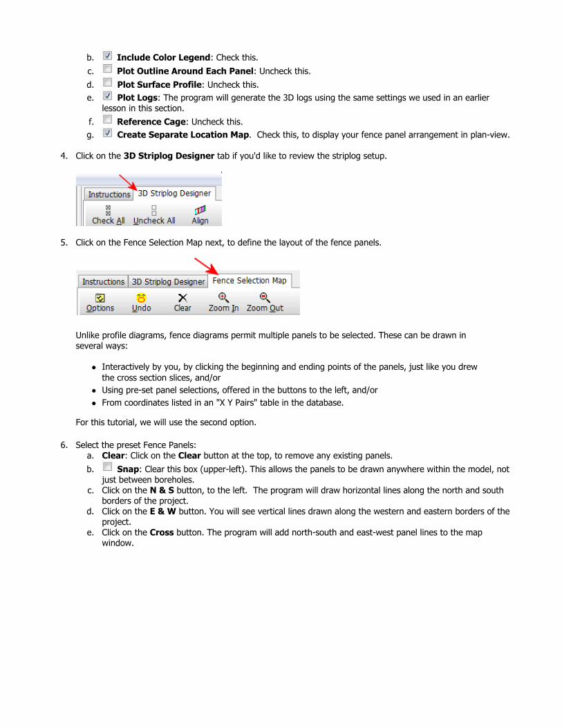
b. Include Color Legend: Check this.
c. Plot Outline Around Each Panel: Uncheck this. d. Plot Surface Profile: Uncheck this. e. Plot Logs: The program will generate the 3D logs using the same settings we used in an earlier
lesson in this section. f. Reference Cage: Uncheck this. g. Create Separate Location Map. Check this, to display your fence panel arrangement in plan-view.
4. Click on the 3D Striplog Designer tab if you'd like to review the striplog setup.
5. Click on the Fence Selection Map next, to define the layout of the fence panels.
Unlike profile diagrams, fence diagrams permit multiple panels to be selected. These can be drawn in several ways:
Interactively by you, by clicking the beginning and ending points of the panels, just like you drew the cross section slices, and/or Using pre-set panel selections, offered in the buttons to the left, and/or From coordinates listed in an "X Y Pairs" table in the database.
For this tutorial, we will use the second option.
6. Select the preset Fence Panels: a. Clear: Click on the Clear button at the top, to remove any existing panels.
b. Snap: Clear this box (upper-left). This allows the panels to be drawn anywhere within the model, not just between boreholes.
c. Click on the N & S button, to the left. The program will draw horizontal lines along the north and south borders of the project.
d. Click on the E & W button. You will see vertical lines drawn along the western and eastern borders of the project.
e. Click on the Cross button. The program will add north-south and east-west panel lines to the map window.

In your own work, you can use any combination of hand-drawn and/or pre-set panel configurations. If you wish to erase the current panels to re-draw, simply click the Clear button to clear the display.! Because the I-Data model is continuous, you can place the fence panels anywhere within the model - you don't have to place the panel endpoints at the borehole locations.
7. Click the Process button at the bottom of the I-Data Fence Diagram window to continue.
The program will read the contents of the existing, already-saved benzene solid model file and will create vertical slices through the model along the indicated panel lines. The completed diagram will be displayed in a RockPlot3D tab. Three-dimensional logs will be appended to the fence diagram. The image is displayed in the pane to the right, and the image components as well as the standard reference items are listed in the pane to the left.
The Fence Location map will be displayed in a separate Rockplot2D tab.
8. Expand the Benzene Soil Fence item in the Data listing. Note that the 6 vertical panels are listed there. Each can be expanded, where the vertical grid model is listed. (If you can’t tell which panel name corresponds to which panel in the view, remove a check-mark and see which one disappears.)
9. Adjust the display as you wish using the Rotate and Pan buttons.
10. Adjust the panel opacity: You can adjust the opacity of an entire group of objects (such as the fence panels) by double-clicking on the Benzene Soil Fence group item. Set the Opacity setting to 70 and click Apply. You should now see the logs better. Close the transparency window.
11. Turn data items on and off: Take a moment to experiment with turning display items on and off, using the check-boxes in the Data listing in the data pane.
12. Save this image: Select the File|Save As command. In the displayed window, type in this name: idata logs+fence and click the Save button. RockPlot3D will save this combined information on disk under that name, with an ".Rw3D" file name extension.
13. Close this plot window by clicking in the Windows Close button in the upper-right corner.
This is the end of the tutorial for interval-based data. The next section contains lessons for time-based interval downhole data.
I-Data Fences
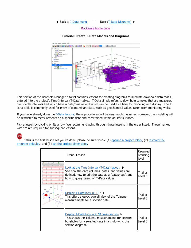
Back to I-Data menu | Next (T-Data Diagrams)
RockWare home page
Tutorial: Create T-Data Models and Diagrams
This section of the Borehole Manager tutorial contains lessons for creating diagrams to illustrate downhole data that’s entered into the project’s Time-Interval (T-Data) tables. T-Data simply refers to downhole samples that are measured over depth intervals and which have a date/time record which can be used as a filter for modeling and display. The T-Data table is commonly used for entry of contaminant data, such as geochemical values taken from monitoring wells.
If you have already done the I-Data lessons, these procedures will be very much the same. However, the modeling will be restricted to measurements on a specific date and constrained within aquifer surfaces.
Pick a lesson by clicking on its arrow. We recommend going through these lessons in the order listed. Those marked with "*" are required for subsequent lessons.
If this is the first lesson set you’ve done, please be sure you’ve (1) opened a project folder, (2) restored the program defaults, and (3) set the project dimensions.
Tutorial LessonRequired licensing level
Look at the Time Interval (T-Data) layout. See how the data columns, dates, and values are defined, how to edit the data as a "datasheet", and how to query based on T-Data values.
Trial orLevel 3
Display T-Data logs in 3D.* This offers a quick, overall view of the Toluene measurements for a specific date.
Trial orLevel 3
Display T-Data logs in a 2D cross section. This shows the Toluene measurements for selected boreholes for a selected date in a multi-log cross section diagram.
Trial orLevel 3

Back to main menu
RockWare home page
Tutorial: View the Time Interval Data Layout
Estimated time: 3 minutes.
In this lesson, you will look at how downhole "Time Interval" or "T-data" is entered, how the columns are defined, how to edit the data as a "datasheet", and how to do a simple query.
1. Be sure the "Samples" folder is still the current project folder (see Open a Project for information).
2. In the borehole file listing along the left side of the Borehole Manager, click on the borehole named DH-14 to
Create a 3D aquifer model.* The surfaces representing the water levels will be used to constrain the time-data model in the following lesson.
Trial orLevel 4
Create a T-data isosurface diagram.* Here you will interpolate the log data into a continuous solid model and display it as an isosurface.
Trial orLevel 4
Create an interpolated T-Data profile. Using the interpolated model from above, you'll display a single slice in a profile diagram, with 2D logs.
Trial orLevel 4
Create a T-Data isosurface diagram for a different date. Here you will quickly create water level surfaces and a new solid T-Data model for a different sampling date.
Trial orLevel 4
Create a morphed model animation. In this lesson you will use the RockWorks morphing tool to create a 3D animation between two toluene models, and to create an AVI file.
Trial orLevel 3
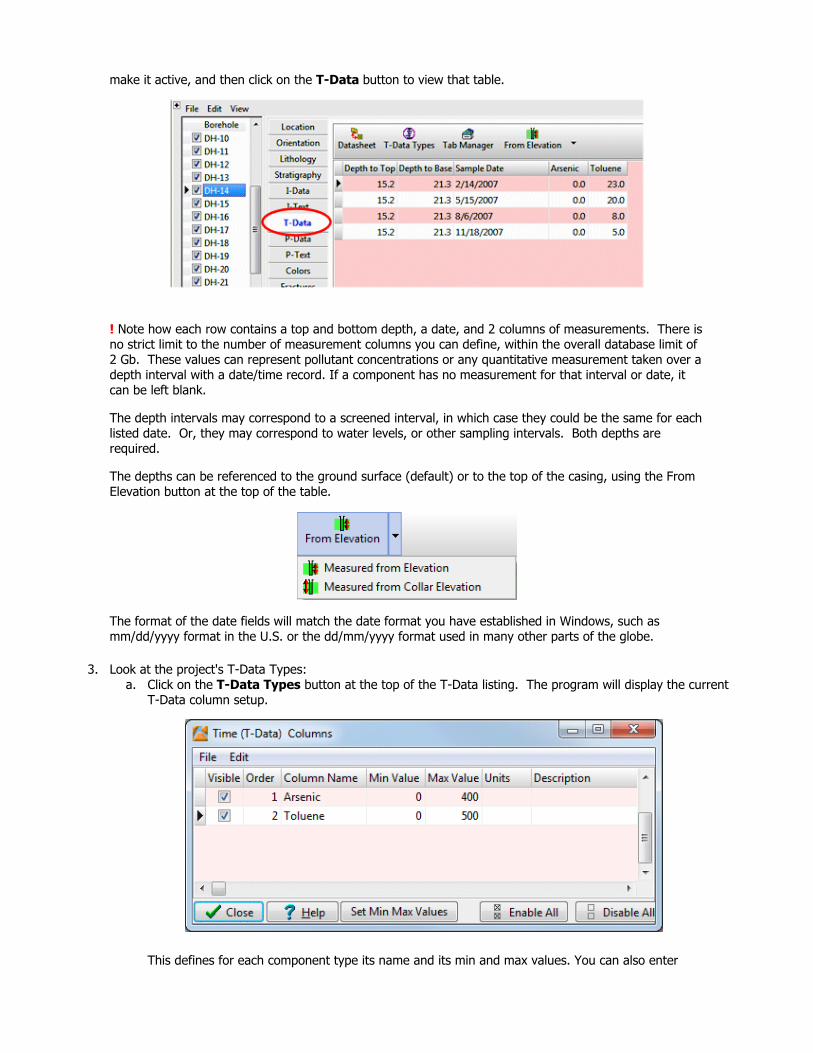
make it active, and then click on the T-Data button to view that table.
! Note how each row contains a top and bottom depth, a date, and 2 columns of measurements. There is no strict limit to the number of measurement columns you can define, within the overall database limit of 2 Gb. These values can represent pollutant concentrations or any quantitative measurement taken over a depth interval with a date/time record. If a component has no measurement for that interval or date, it can be left blank.
The depth intervals may correspond to a screened interval, in which case they could be the same for each listed date. Or, they may correspond to water levels, or other sampling intervals. Both depths are required.
The depths can be referenced to the ground surface (default) or to the top of the casing, using the From Elevation button at the top of the table.
The format of the date fields will match the date format you have established in Windows, such as mm/dd/yyyy format in the U.S. or the dd/mm/yyyy format used in many other parts of the globe.
3. Look at the project's T-Data Types: a. Click on the T-Data Types button at the top of the T-Data listing. The program will display the current
T-Data column setup.
This defines for each component type its name and its min and max values. You can also enter
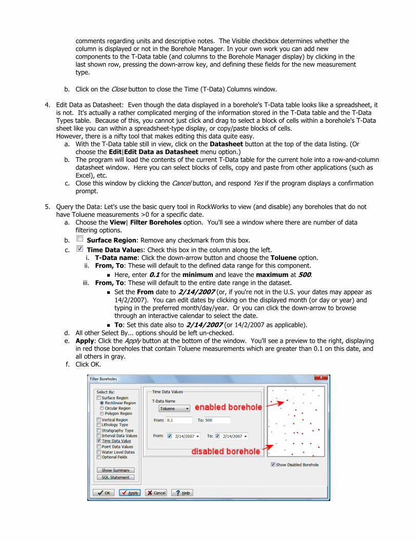
comments regarding units and descriptive notes. The Visible checkbox determines whether the column is displayed or not in the Borehole Manager. In your own work you can add new components to the T-Data table (and columns to the Borehole Manager display) by clicking in the last shown row, pressing the down-arrow key, and defining these fields for the new measurement type.
b. Click on the Close button to close the Time (T-Data) Columns window.
4. Edit Data as Datasheet: Even though the data displayed in a borehole's T-Data table looks like a spreadsheet, it is not. It's actually a rather complicated merging of the information stored in the T-Data table and the T-Data Types table. Because of this, you cannot just click and drag to select a block of cells within a borehole's T-Data sheet like you can within a spreadsheet-type display, or copy/paste blocks of cells.However, there is a nifty tool that makes editing this data quite easy.
a. With the T-Data table still in view, click on the Datasheet button at the top of the data listing. (Or choose the Edit|Edit Data as Datasheet menu option.)
b. The program will load the contents of the current T-Data table for the current hole into a row-and-column datasheet window. Here you can select blocks of cells, copy and paste from other applications (such as Excel), etc.
c. Close this window by clicking the Cancel button, and respond Yes if the program displays a confirmation prompt.
5. Query the Data: Let's use the basic query tool in RockWorks to view (and disable) any boreholes that do not have Toluene measurements >0 for a specific date.
a. Choose the View| Filter Boreholes option. You'll see a window where there are number of data filtering options.
b. Surface Region: Remove any checkmark from this box. c. Time Data Values: Check this box in the column along the left.
i. T-Data name: Click the down-arrow button and choose the Toluene option. ii. From, To: These will default to the defined data range for this component.
Here, enter 0.1 for the minimum and leave the maximum at 500. iii. From, To: These will default to the entire date range in the dataset.
Set the From date to 2/14/2007 (or, if you're not in the U.S. your dates may appear as 14/2/2007). You can edit dates by clicking on the displayed month (or day or year) and typing in the preferred month/day/year. Or you can click the down-arrow to browse through an interactive calendar to select the date. To: Set this date also to 2/14/2007 (or 14/2/2007 as applicable).
d. All other Select By... options should be left un-checked. e. Apply: Click the Apply button at the bottom of the window. You'll see a preview to the right, displaying
in red those boreholes that contain Toluene measurements which are greater than 0.1 on this date, and all others in gray.
f. Click OK.

Back at the Borehole Manager, you'll see a number of boreholes are now shown as inactive - they are no longer shown with check-marks. Disabled boreholes will not be displayed in maps or log displays, and their data will not be included in any modeling. We will leave some of these boreholes disabled for the next lesson only.
! The View | Filter Boreholes option uses an "AND" type of query, in which each of the boreholes for which every criterion is true will be enabled and the remaining boreholes will be disabled. The View | Select Boreholes option is more complex, allowing successive filters to be applied, and the enabling/disabling will apply only to the boreholes meeting the filter parameters, and no others. So, while the Filter Boreholes tool works as an AND filter, the Select Boreholes tool can function as an AND or OR filter.
Entering T-Data
Back to T-Data menu | Next (3D logs)
RockWare home page
Tutorial: Display T-Data Logs in 3D
Estimated time: 4 minutes.
In this lesson, you will get a quick view of Toluene measurements for a single date, as entered for the project's boreholes, by generating 3D logs for the currently-enabled boreholes.
1. To create the 3D logs, click on the Striplogs menu, and choose 3-Dimensional and Multiple Logs.
This window has several sections:The left side is where general diagram settings are established.The 3D Striplog Designer tab is where you establish the log-specific settings.
2. Establish the general diagram settings in the left pane. Group Title: This can be left at: Logs
Clip: Uncheck this.
Reference Cage: Uncheck this.
Include Lithology Legend: Uncheck this.
Include Stratigraphy Legend: Uncheck this.
Include Well Construction Legend: Uncheck this.
3. Click on the 3D Striplog Designer tab.
The left pane of this tab is where you choose what type of data is to be displayed in the logs (the Visible Items). The upper-right pane is where you see a plan-view Preview of the active log items. You can drag the items to adjust their relative placement. The lower-right pane displays specific Options for the Visible Item that you click on.
4. Choose the items you want to see in the logs by inserting a check-mark in the following items in the Visible Items section of the window:

Title: The drill hole name will plot above the logs. Axis: The logs' axes will be shown with a solid line. T-Data #1: The logs will contain a column illustrating time-interval measurements. You can include
up to 4 different T-Data components or dates; we'll display only one in this lesson.When this column is selected, you'll see a green circle displayed in the plan-view Preview pane.
Track: At the top of the Options pane, click on the Track heading and choose Toluene as the data to be represented in the logs. Expand the Track heading to access the data filter options.
Filter Based on G Values: Be sure this is left un-checked. In your own work this can be used to display only high or low values in your logs.
Resample at Regularly-Spaced Intervals: Be sure this is also left un-checked. In your own work, these settings can be used to thin the number of downhole measurements displayed (for densely sampled drillholes) or to include zero-value "bogus" points to add control to sparsely-sampled holes.
Column Title: This should be blank. If text is displayed for this prompt, click on this heading and delete the text.
Plot Interval Labels: Leave this unchecked (it's used to plot value labels down the log). Offset Direction: This should reflect the current offset, in azimuth degrees, from the axis of the log. It can be left at zero. Offset Distance: Adjust the placement of the column relative to the axis of the log by dragging the circle in the Preview pane. Be sure the T-Data circle is on the center of the log axis.! You can simply type 0.0 into the Offset Distance prompt, if you prefer. Column Radius: You can adjust the size of the column by dragging on one of the corner handles. Note the Column Radius setting in the lower-right Options pane. As you resize the circle, the Radius setting will be updated. Drag the T-Data #1 circle until the Column Radius is about 2.0.! You can also simply type 2.0 into the Column Radius prompt. Scaling: Expand this heading and select Automatic. Fill Style: Expand this Options heading, and choose Variable. This will color-code the logs based on Cobalt values. Shape: Expand this Options heading, and choose Cylinders.
None of the other Visible Items should be checked. Here's a summary of these settings:

5. Now, set up the date filter for these T-Data logs, using the Rules and Filters pane to the right. Date / Time Filtering: Insert a check in this box to activate a date filter.
Exact: Click in this radio button and click on the Date/Time Target prompt. Set the target date to 2/14/2007 (or 14/2/2007 for non-U.S. date formats). You can edit dates by clicking on the displayed month (or day or year) and typing in the preferred month/day/year. Or you can click the down-arrow to browse through an interactive calendar to select the date.
6. Click the Process button at the bottom of the window to proceed.
The program will create a log for each enabled borehole, including well name at the top, and color-coded

Toluene cylinders displayed down the log. They will be displayed in a new, RockPlot3D tab.
The image is displayed in the pane to the right, and the image components as well as the standard reference items are listed in the pane to the left of the image. The expandable/collapsible list on the left is called the "data tree."
7. Adjust the reference items: World Outline: Turn on the World Outline, by inserting a check in its check-box in the upper portion
of the left-hand listing. You can expand the World Outline heading to specify which world items are enabled.
Base: Turn on only the Base item - the remaining items can be unchecked. Axes: Be sure the 3D axes are turned on. Labels: Turn on the axis labels using this check box.
8. Adjust the zoom: Click in the drop-down Zoom box on the toolbar, and choose 200%.
9. Re-adjust the rotation if you wish, even when zoomed in. Use the Pan tool to move the current view back
and forth, up and down. To zoom back out, just click once on the Zoom Out button .
10. Turn on/off logs: Expand the Logs item in the data tree to the left, to see the individual boring names. You can turn entire logs on and off simply by checking/clearing their respective check-boxes. Try this for a few borings.
11. Turn on/off log items: In addition, if you expand an individual borehole in the data list, you’ll see its title, axis, and data groups. These, also, can be turned on and off for each well.
12. Save this 3D log data: Select the File | Save As command. In the displayed window, type in this name: toluene logs 2-14-07 and click the Save button. RockPlot3D will save this information on disk under that name, with an ".Rw3D" file name extension. In later lessons, you can append these logs to other 3D diagrams.

13. Close the RockPlot3D window by clicking in the Windows Close button .
3D Logs
Back to T-Data menu | Next (2D log section)
RockWare home page
Tutorial: Display Multiple T-Data Logs in a 2D Cross-Section
Estimated time: 4 minutes.
In this lesson, you will be creating an image representing the Toluene T-Data measurements in multiple logs in the Samples project, selected along a multi-log cross section trace.
1. Re-enable all of the boreholes in the project by clicking on the Edit | Enable All Boreholes menu option or toolbar button.
2. Click on the Striplogs menu, and then click on 2-Dimensional | Section. (What's the difference between "profiles," "sections," and "projected sections"? Click here.)
3. Establish the section options:These are found in the left pane of the Hole-to-Hole Log Section window. Plot Striplogs: Check this.
Borehole Spacing: Expand this heading to confirm that this is set to Distance between Collar Locations.
Plot Correlations: Uncheck this.
Hang Section on Datum: Uncheck this.
or Plot Surface Profile: If you completed the borehole map section of the tutorial (jump back), insert a check in the Plot Surface Profile option. This is used to display a selected surface in the cross section plot. If you DID NOT complete that lesson, leave this un-checked.
Grid Model: Click here and select the RwGrd file representing the ground surface, named surface.RwGrd and click the Open button. Line Type: Click here to set the line style to red, medium thickness. Smoothing can be set to 1.
Show Fault(s): Uncheck this.
Perimeter Annotation Options: These options determine text and lines that will plot around the perimeter of the profile. Click on this button to view the options; the factory defaults should be fine. See Restore Default Settings if you need more information about setting the factory defaults.! In your own work the Intended Vertical Exaggeration Factor can be very helpful for good diagram proportions if you have a large, flat study area and will stretch your cross sections for readability.
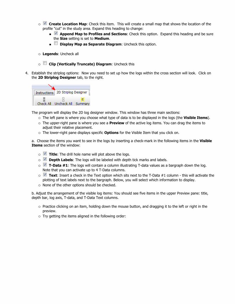
Create Location Map: Check this item. This will create a small map that shows the location of the profile "cut" in the study area. Expand this heading to change:
Append Map to Profiles and Sections: Check this option. Expand this heading and be sure the Size setting is set to Medium.
Display Map as Separate Diagram: Uncheck this option.
Legends: Uncheck all
Clip (Vertically Truncate) Diagram: Uncheck this
4. Establish the striplog options: Now you need to set up how the logs within the cross section will look. Click on the 2D Striplog Designer tab, to the right.
The program will display the 2D log designer window. This window has three main sections: The left pane is where you choose what type of data is to be displayed in the logs (the Visible Items). The upper-right pane is where you see a Preview of the active log items. You can drag the items to adjust their relative placement. The lower-right pane displays specific Options for the Visible Item that you click on.
a. Choose the items you want to see in the logs by inserting a check-mark in the following items in the Visible Items section of the window:
Title: The drill hole name will plot above the logs. Depth Labels: The logs will be labeled with depth tick marks and labels. T-Data #1: The logs will contain a column illustrating T-data values as a bargraph down the log.
Note that you can activate up to 4 T-Data columns. Text: Insert a check in the Text option which sits next to the T-Data #1 column - this will activate the
plotting of text labels next to the bargraph. Below, you will select which information to display. None of the other options should be checked.
b. Adjust the arrangement of the visible log items: You should see five items in the upper Preview pane: title, depth bar, log axis, T-data, and T-Data Text columns.
Practice clicking on an item, holding down the mouse button, and dragging it to the left or right in the preview. Try getting the items aligned in the following order:
! Note that the log axis is always activated. It acts as the "anchor" point for the log - it's the axis that will be placed at the actual log location in the diagrams. The log title is always placed atop the axis.
c. Check the options for each visible item by clicking on the item's name in the listing; its options will be displayed in the Options pane.
Click on the T-Data #1 item.
Track: Click here and choose Toluene from the list. Expand this heading.
Filter Based on G Values: Leave this un-checked.
Resample at Regularly-Spaced Intervals: Leave this un-checked.
Note that the Date filter, in the Rules & Filters pane to the right, should still be set to Exact, for 2/14/2007.

Width: Click on this item, and set the Width to 2. ! All log item sizes are expressed as a percent of the dimensions of the project, so the width of these logs will be about 1% of the project dimensions. Column Title: Click on this option in the right-hand pane.
Type in: TolueneExpand this heading.
Include Data Range: Check this item, and expand its heading to set the decimal places to 0.
Column Perimeter: This can be left unchecked. Background Subdivisions: Check this box, and expand this heading.
Intervals: Set to 5. Plotting Sequence: Expand this and choose Background.
Scaling: Set this to Automatic. Fill Style: Scroll down to find this heading in the Options pane.
Monochrome: Choose this Fill Style option and set the color to blue. Direction: Look for this heading in the Options pane.
Left-to-Right: Choose this option.
Click on the Text column item to bring up its options.
Width: Set this to 4. Dates: Insert a check here to display the date fields. T-Data Values: Insert a check here to display the T-Data values themselves.
Font: Click on this item and set the Size to 0.75. All of the other text options can be left unchecked.
5. Next, pick the boreholes to display. Click on the Section Selection Map tab.
If you don't see the section trace pictured below, follow these steps; otherwise jump to #6 below. Click on the Clear button at the top of the panel-picking window. The program remembers your cross
section traces from session to session; this will clear any old traces from memory. Next, locate the hole titled "DH-17" (in the upper-left) and click on it. It will be marked with a red "X". Locate hole "DH-03" just southeast of "17" and click on it. A line will be drawn between the holes. Locate hole "DH-21" southeast of "03" and click on it.! If you make a mistake, click the Undo button to undo the last pick or the Clear button to clear the slate for starting over. Click on "DH-40," "DH-41," and "DH-07," continuing the cross section across the project area. You should see a trace like this:
6. Click the Process button at the bottom of the Hole to Hole Log Section window to proceed.
The program will create strip logs of each of the selected borings using the selected settings. The logs will be spaced proportionally to their distance from each other on the ground.In addition, it will create a map that displays the location of the section slice within the study area.
The completed log section and location map will be displayed in a RockPlot2D tab, where 2-dimensional ("flat") maps and other diagrams are presented.
7. Enlarge the display window by hiding the left-hand menu: click on the small "-" button in the middle of the divider bar. The program will rescale the image within the resized window.

8. Zoom into the view: Since the labels appear fairly small, use the Zoom toolbar button to enlarge the logs in the middle of the section.
a. Click on the Zoom button. b. Draw a zoom rectangle around the logs:
You can use the scroll bars to the right of and below the display to adjust the portion of the image that's in view.
! If you zoom in really far - "super-zoom" state - the scroll bars will no longer be displayed. You
can use the Undo Last Zoom button to step back outward in your zoom sequence.
9. Edit a log label. a. Pan and Zoom to the T-Data value label that is displayed on DH-40, which has the largest bargraph
value.
b. Click the RockPlot Edit button in the upper toolbar. c. Double-click on the label to be edited (or right-click on the label and choose Properties). d. Change the font color setting to red. e. Change the font Background: Click in the Opaque option and set the color to Yellow. f. Click the OK button. g. You will see the label colors change in the display.
10. Click the Zoom Out button to return to full view.
11. Experiment with the layers: a. If the Layers pane is not visible to the right of the display, click on the small "+" button in the upper-right
corner of the plot pane. b. Remove/insert the check-mark from any of the layers, to see how they disappear from the display. c. Right-click on any layer in the list and choose Select Layer, and the layer will be shown as selected (with
"handles") in the display.

d. In your own work, you can right-click on any layer in the list and choose Delete to remove the layer from the diagram permanently.
12. Save the cross section image for later overlay with another section diagram. a. With the section still displayed in the RockPlot window, choose File | Save, and type in the name:
toluene log section 2-14-07 and click Save. The program will save this image in its own ".Rw2D" file format.
b. You can close this RockPlot window by clicking in the standard Windows close-window button .
See also: RockPlot2D tutorial
Displaying Multiple Logs in a 2D Hole to Hole Section
Back to T-Data menu | Next (aquifer model)
RockWare home page
Tutorial: Create a 3D Aquifer Model
Estimated time: 4 minutes.
We are going to take a slight detour at this time to create a model of the water level data in the borehole project. These surfaces will be used in the next lesson to constrain the T-Data model.
An aquifer model is created by interpolating 2 grid surfaces (.RwGrd): one for the water level top and one for the base.
! You must be using RockWorks in Trial mode, or have a Level 4 or 5 license to run this modeling program.
Before continuing, be sure you have opened the sample project, and established the project dimensions, as discussed in earlier lessons.
1. Re-enable all of the boreholes in the project, if necessary, by clicking on the Edit | Enable All Boreholestoolbar button or selecting that menu option.
2. Look at the aquifer data: a. Back at the Borehole Manager, click on any borehole to make it active. b. Click on its Water Levels button to view the aquifer data. c. Note how this table contains only 4 columns:
Aquifer Name: Since you can include multiple aquifers in your database, the first column defines which aquifer's data you are entering. The names are defined in the Aquifer Types Table. You can click on this button, above the data listing, to see the types table. Date of Sample: Just like the T-Data, water levels are also flagged with dates. Depth to Top: Measured depth from the borehole surface to the aquifer top. Depth to Base: Measured depth to the aquifer base.
d. At the top of the Water Levels table, there is a From Elevation / From Collar button - you can use this in your own work to define whether the water level depths (for all holes) are referenced to the ground surface elevation or the collar elevation, both listed on the Location table.
3. Establish the modeling settings: Select the Aquifers | Model menu option. Choose Aquifers:
Single Aquifer: Choose this option, and be sure this is set to Aquifer 1.
Surface Modeling: Expand this heading to define how the surfaces will be modeled.
Gridding Options: Click on this button to access the gridding settings. Method (Algorithm): Choose the Inverse Distance option. This tells the program to use the Inverse-Distance gridding method to interpolate the aquifer surfaces. The default settings for this algorithm will be fine. Dimensions: This item (upper-right) should be set to be Based on Output Dimensions.
Smooth: Check this option to smooth the resulting surfaces.
All remaining Additional Options can be left unchecked. Click the OK button to close the Gridding Options window.
Hide Thin Zones: Leave this setting unchecked. (In your own work it can be used to hide portions of the aquifer model that are below a user-defined thickness.)
Plot Logs: Leave this setting unchecked.
Reference Cage: Leave this setting unchecked.
Rules & Filters: : Look for the Rules & Filters pane along the right side of the options window. Date/Time Filtering: Be sure this is checked. Exact: Click in this radio button.
Click in the prompt to set this date to 2/14/2007 (or, if you're not in the U.S. your dates may appear as 14/2/2007).
4. Click Process at the bottom of the Aquifer Modeling window.
RockWorks will read the aquifer top and base depths, determine true elevations, and create a grid model for each that represents the water level surface. The upper surface will be stored under the name "2_14_2007_top.RwGrd," named automatically by the program (the name will be formatted as "14_2_2007.RwGrd" if that is your date format). The lower surface will be stored under the name "2_14_2007_base.RwGrd". You'll use these RwGrd files in the next lesson.
Once the surfaces are interpolated and stored on disk, the program will create a 3D view of aquifer and display it in a RockPlot3D window.
5. If you would like to take a moment to investigate this view (zoom, rotate, expand the "2/14/2007 Water" item in the data tree, turn portions on/off, etc.) feel free to do so.
6. Save this 3D view by choosing File | Save and typing in the name: aquifer model 2-14-07 The program will store this under the file name "aquifer model 2-14-07.Rw3D".
7. Close this RockPlot3D window by clicking in its upper-right Close box.
Creating Water Level Models
Back to T-Data menu | Next (isosurface diagram)
RockWare home page
Tutorial: Create a T-Data Model and Isosurface Diagram
Estimated time: 5 minutes.
Now we will jump from the Striplogs menu, where we plotted observed data in log diagrams, and the Aquifers menu, where we interpolated water surface models, to the T-Data menu, where the downhole quantitative data will be interpolated into a continuous solid model.
In this lesson, you will create a solid model and 3-dimensional isosurface diagram of the project's Toluene measurements, for a specific date. The program will load the recorded borehole data, that you viewed in logs and log
sections already, and extrapolate the measured values throughout the project. This modeling process basically "fills in the blanks" between the logs. RockWorks offers several modeling algorithms to do this extrapolation; sparse time-based data typically requires a different modeling technique than denser data might.
Before continuing, be sure you have opened the sample project, established the project dimensions, created 3D logs, and created an aquifer model as discussed in earlier lessons.
1. Back at the Borehole Manager, click on the T-Data menu and select the Model option.
2. Establish the modeling settings: Create New Model: Click in this button, and expand this item.
T-Data Track: Click here to select the column titled Toluene from the pop-up list. Expand this heading to set the input data filters.
Filter based on G-Values: Leave this unchecked.
Resample at Regularly-Spaced Intervals: Leave this unchecked.
Solid Model Name: Click to the right to assign a name for the interpolated model, and type in: toluene 2-14-07This will be the name assigned to the solid model to be created, with an ".RwMod" file name extension. ! Note how you've included the date in the model name - this can be handy to keep track of which solid model represents which date measurements. RockWorks does not assign these names automatically.
Solid Modeling Options: Click on the Options button to the right to establish the modeling settings. Algorithm (Modeling Method): ! For Time Interval Data, this is important. The default method that RockWorks uses for general solid modeling is Inverse Distance Anisotropic. While this works well for numerous I-Data measurements, this isn't the best choice for the limited measurements typical of T-Data.
IDW Advanced: Click in this radio button; note that modeling options are displayed to the right.
Weighting Exponents: These options allow you to vary the influence of measurements that lie horizontally versus vertically in relation to each node being interpolated. The greater the exponent value, the less influence the measurements will have.
Horizontal: Set this exponent to 2. (normal influence) Vertical: Set this exponent to 4. (reduced influence)
Search Method: Expand this heading. All Points: Choose this option so that the program will not limit the search
for measurements to consider when interpolating the node values.
Additional Options:Dimensions: These define the extents of the output model.
Based on Output Dimensions: Be sure this option is checked.
Confirm Model Dimensions item can be left unchecked (though in your own work, this is a handy way to double-check the model extents and node spacing).
Decluster: Unchecked.
Add Points: unchecked.
Cutoff - H, Cutoff - V: unchecked.
LogarithM: unchecked. If used, this can be helpful for interpolation of highly anomalous data.
Smoothing: unchecked.
HiFi: unchecked.
Distance: unchecked.
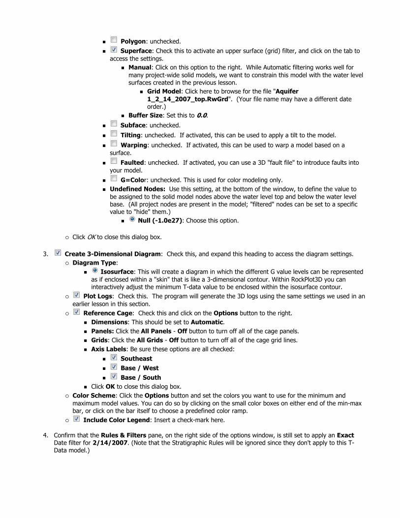
Polygon: unchecked. Superface: Check this to activate an upper surface (grid) filter, and click on the tab to
access the settings. Manual: Click on this option to the right. While Automatic filtering works well for many project-wide solid models, we want to constrain this model with the water level surfaces created in the previous lesson.
Grid Model: Click here to browse for the file "Aquifer 1_2_14_2007_top.RwGrd". (Your file name may have a different date order.)
Buffer Size: Set this to 0.0.
Subface: unchecked.
Tilting: unchecked. If activated, this can be used to apply a tilt to the model.
Warping: unchecked. If activated, this can be used to warp a model based on a surface.
Faulted: unchecked. If activated, you can use a 3D "fault file" to introduce faults into your model.
G=Color: unchecked. This is used for color modeling only.Undefined Nodes: Use this setting, at the bottom of the window, to define the value to be assigned to the solid model nodes above the water level top and below the water level base. (All project nodes are present in the model; "filtered" nodes can be set to a specific value to "hide" them.)
Null (-1.0e27): Choose this option.
Click OK to close this dialog box.
3. Create 3-Dimensional Diagram: Check this, and expand this heading to access the diagram settings. Diagram Type:
Isosurface: This will create a diagram in which the different G value levels can be represented as if enclosed within a "skin" that is like a 3-dimensional contour. Within RockPlot3D you can interactively adjust the minimum T-data value to be enclosed within the isosurface contour.
Plot Logs: Check this. The program will generate the 3D logs using the same settings we used in an earlier lesson in this section.
Reference Cage: Check this and click on the Options button to the right. Dimensions: This should be set to Automatic. Panels: Click the All Panels - Off button to turn off all of the cage panels. Grids: Click the All Grids - Off button to turn off all of the cage grid lines. Axis Labels: Be sure these options are all checked:
SoutheastBase / WestBase / South
Click OK to close this dialog box. Color Scheme: Click the Options button and set the colors you want to use for the minimum and maximum model values. You can do so by clicking on the small color boxes on either end of the min-max bar, or click on the bar itself to choose a predefined color ramp.
Include Color Legend: Insert a check-mark here.
4. Confirm that the Rules & Filters pane, on the right side of the options window, is still set to apply an ExactDate filter for 2/14/2007. (Note that the Stratigraphic Rules will be ignored since they don't apply to this T-Data model.)

Spatial (XYZ) Filtering: Leave this unchecked.
5. Click the Process button at the bottom of the T-Data Model window. RockWorks will create two items:
It will interpolate a solid model using the specified project dimensions using the IDW Advanced method of extrapolating the Toluene concentrations for those areas with no boreholes, using the date-filtered input data. Nodes which lie above the constraining water surface will be assigned a Null value. The completed model will be store in the project folder with the name "toluene 2-14-07.RwMod."
RockWorks will then create an isosurface diagram to illustrate the model. The completed diagram will be displayed in a RockPlot3D tab.
6. View the isosurface model options by double-clicking on the Toluene item that’s listed in the data tree.
The program will display a window listing the Isosurface Options. Here’s a quick summary:
Color scheme: This solid model contains "G" values representing Toluene concentrations that range from a minimum to a maximum. The default scheme will be set to Continuous, to show continuous gradations between the low and high values. If you wish, you can change the by clicking on the Min-Max

button to the right of the color scheme. In your own work, if you want to display specific concentrations using specific colors you can use the Color Table option, for which you create a table that lists G value ranges and the colors to represent them. Draw Style: Default is Solid. You might try changing the display to Wire Frame to see the effect. Click the Apply button at the bottom of the window to make any changes you set take effect. Using Wire Frame can speed rendering of the solid if it is dense or your computer system is slow. Opacity: You’ll see this one in most 3D Options windows. You can make the block more transparent by reducing the percent opacity shown here. Again, use Apply to see changes take effect. Plot Outline: This draws an outline around the boundary of the model. Cap Style: This tells the program how you want the "blobs" that intersect the edge of the model to be displayed. By changing the contour interval, you can see how the concentrations change inside the isosurface. Iso-level: This allows you to see only selected G values in the block. See #7 below. Slices: This allows you to see insert horizontal or vertical slices at specific locations in the block.
If you have a minute, you should go through the next few steps to learn some of the ins and outs of viewing isosurface diagrams. If you are in a hurry, you can review these lessons later in the dedicated RockPlot3D tutorial.
7. Change the iso-level being displayed: Find the slider bar in the Iso-Level section. The left-hand value on this slider corresponds to the minimum Toluene concentration, and the right-hand value represents the maximum concentration. Drag the slider bar slowly to the right, with the intention of changing the minimum Toluene level displayed, to see how the display changes. In your own work you can use the slider or just type a minimum desired value into the prompt. Try typing: 40 into the Iso-Level Value prompt and clicking Apply.
Note that you can Rotate or Pan the image at any time without closing the Options window to get a better view. Or, use the View | Above or Below or Compass Points tools to return to a pre-set view.
8. Show the current volume: Insert a check in the Show Volume check-box and the program will display right in the Options window the total volume in the model at the minimum Toluene concentration and above. If you drag the slider bar to change the minimum isosurface, the volume will change.
9. Adjust the transparency: To see through the isosurface to the logs inside, which represent the observed data values, set the Opacity value to 70 and click Apply.
10. Save the current scene: Choose File | Save and type in this name: toluene 2-14-07RockPlot3D will append the ".Rw3D" file name extension automatically.
11. Close this RockPlot3D window by clicking in its upper-right Close box .

Solid Modeling Reference, Creating T-Data Models
Back to T-Data menu | Next (interpolated cross section)
RockWare home page
Tutorial: Create a Modeled T-Data Profile
Estimated time: 3 minutes.
In this lesson, you will create a single-panel cross section slice using the same T-data model used previously for the isosurface diagram.
! The instructions below are written with the assumption that you have completed the previous lesson, as well as the lesson on log sections.
1. Click on the T-Data Menu and choose Profile.
2. Establish the modeling settings:Use Existing Model: Since you took the time to create a T-data solid model in the previous lesson, we can
use that one for this tutorial. Expand this item.Model Name: Click here to browse for the file "toluene 2-14-07.RwMod".! This is important to remember in your own work. Once a solid, numerical model is created to represent your data, and saved on disk as an .RwMod file, you can use that same model to create different types of diagrams – profiles, sections, fences, isosurfaces, slices – without having to reinterpolate the solid model each time.
3. Establish the diagram options: a. Contour Lines: Uncheck this. b. Colored Intervals: Check this. c. Plot Logs: The program will project 2D logs onto the profile panel. If you want to review the 2D log
settings (which you established in for the striplog section) you click on the 2D Striplog Designer tab to the right.
d. Plot Surface Profile: This option can be either checked or not, as per the log section lesson.
e. Create Additional Parallel Profiles: Uncheck this. f. Show Faults: Uncheck this. g. Perimeter Annotation: The defaults from the earlier lesson should work. h. Create Location Map.
4. Next, establish the Profile location. Click on the Profile Selection Map tab. Any previous profile trace that you may have drawn in a separate session will be displayed.

Select the profile location: Select the starting point for the profile cut by clicking on the borehole DH-30 near the northwest corner of the project area. Select the endpoint for the profile (you're picking a single slice only) by clicking on the borehole DH-23 in the middle of the eastern side of the project. Be sure that the swath to either side of the slice, within which the logs will be projected onto the diagram, is set to 20. This swath is represented by the yellow cross-hatching, as shown below.
5. Click the Process to accept the modeling and diagram options, and the profile location.
The program will read the existing solid model (toluene 2-14-07.RwMod) and extract a panel along the indicated profile trace, with the indicated perimeter annotation. The bargraph logs will be projected perpendicularly onto the profile diagram. The map representing the panel trace will appended to the profile. The completed diagram will be displayed in a RockPlot2D window.
6. You can use the check-boxes in the Layers pane to the right to turn on/off specific logs (or portions of logs which are projected onto the profile), panels, etc.
7. You can save the section if you want, using the File | Save As menu command and entering a name of your choice.
8. Close the profile window.
T-Data Profiles
Back to T-Data menu | Next (model new date)
RockWare home page
Tutorial: Create a T-Data Model for another Date
Estimated time: 4 minutes.

The next two lessons are designed to show you how to create an Aquifer model and T-Data model for the measurements from a different date (following the same steps you've already gone through), and then morph the models into a "continuous" animation view.
Before continuing, be sure you have completed the earlier lesson - creating a T-Data isosurface.
1. Select the Aquifers | Model menu option to create the water surfaces for a new date. Choose Aquifer(s)
Single Aquifer - Aquifer 1: Be sure this option is still selected.
Hide Thin Zones: Uncheck.
Plot Logs: Uncheck.
Reference Cage: Uncheck.
Rules & Filters: In the right-hand pane of the options window, change the Exact date filter to 11/18/2007 (or, if you're not in the U.S. your dates may appear as 18/11/07).
2. Click Process at the bottom of the Aquifer Modeling window.
The program will interpolate the water surface grids for this date and store them in the project folder. It will display the surfaces in a RockPlot3D window.
3. Close the window; you do not need to save this view.
4. Back at the Borehole Manager, click on the T-Data menu and select the Model option.
5. Establish the modeling settings: Create New Model: Click in this button, and expand this item.
T-Data Track: Be sure this is still set to the column titled Toluene.
Solid Model Name: Click here to assign a name for the interpolated model, and type in: toluene 11-18-07
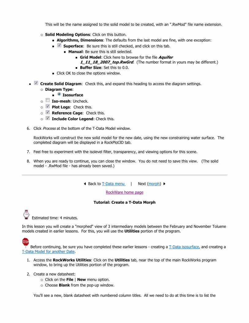
This will be the name assigned to the solid model to be created, with an ".RwMod" file name extension.
Solid Modeling Options: Click on this button. Algorithms, Dimensions: The defaults from the last model are fine, with one exception:
Superface: Be sure this is still checked, and click on this tab. Manual: Be sure this is still selected.
Grid Model: Click here to browse for the file Aquifer 1_11_18_2007_top.RwGrd. (The number format in yours may be different.) Buffer Size: Set this to 0.0.
Click OK to close the options window.
Create Solid Diagram: Check this, and expand this heading to access the diagram settings. Diagram Type:
IsosurfaceIso-mesh: Uncheck. Plot Logs: Check this. Reference Cage: Check this. Include Color Legend: Check this.
6. Click Process at the bottom of the T-Data Model window.
RockWorks will construct the new solid model for the new date, using the new constraining water surface. The completed diagram will be displayed in a RockPlot3D tab.
7. Feel free to experiment with the isolevel filter, transparency, and viewing options for this scene.
8. When you are ready to continue, you can close the window. You do not need to save this view. (The solid model - .RwMod file - has already been saved.)
Back to T-Data menu | Next (morph)
RockWare home page
Tutorial: Create a T-Data Morph
Estimated time: 4 minutes.
In this lesson you will create a "morphed" view of 3 intermediary models between the February and November Toluene models created in earlier lessons. For this, you will use the Utilities portion of the program.
Before continuing, be sure you have completed these earlier lessons - creating a T-Data isosurface, and creating a T-Data Model for another Date.
1. Access the RockWorks Utilities: Click on the Utilities tab, near the top of the main RockWorks program window, to bring up the Utilities portion of the program.
2. Create a new datasheet: Click on the File | New menu option. Choose Blank from the pop-up window.
You'll see a new, blank datasheet with numbered column titles. All we need to do at this time is to list the

names of the two given RwMod files between which the morphed intermediates will be generated. One method is to type the model names into the cells of the datasheet. But, easier (and less prone to mistakes) is to browse for the file names, interactively. This requires setting the cells to a "File" type.
3. Right-click in the upper (gray) portion of column 1. (Or select the Columns | Column Properties menu option.) The program will display a window that looks like this:
Change the Title for Column 1 to: Model NameDo this simply by clicking in the uppermost Title cell and replacing the "1" with "Model Name" For the data type for Column 1 click in the File Name radio button. Click OK at the bottom of the window to accept these changes.
You'll see the new column name at the top of the first column.
4. Select the RwMod file names: Double-click in the first row under the new Model Name column. Since you just set this column to a "File" type, RockWorks will retrieve a browse window. Browse for the name of the first T-Data model you generated, named toluene 2-14-07.RwMod. Click on this model name and click the Open button. You'll see this name in the first row. Double-click in the second row under the Model Name columns. Browse for the name of the second T-Data model you generated, named toluene 11-18-07.RwMod. Click on this model name, and click Open. You'll see this name in the second row.
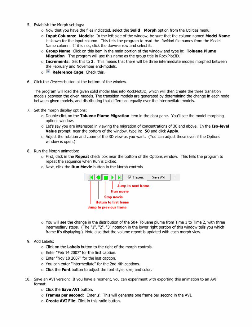
5. Establish the Morph settings: Now that you have the files indicated, select the Solid | Morph option from the Utilities menu. Input Columns: Models: In the left side of the window, be sure that the column named Model Nameis shown for the input column. This tells the program to read the .RwMod file names from the Model Name column. If it is not, click the down-arrow and select it. Group Name: Click on this item in the main portion of the window and type in: Toluene Plume Migration The program will use this name as the group title in RockPlot3D. Increments: Set this to 3. This means that there will be three intermediate models morphed between the February and November end-models.
Reference Cage: Check this.
6. Click the Process button at the bottom of the window.
The program will load the given solid model files into RockPlot3D, which will then create the three transition models between the given models. The transition models are generated by determining the change in each node between given models, and distributing that difference equally over the intermediate models.
7. Set the morph display options: Double-click on the Toluene Plume Migration item in the data pane. You'll see the model morphing options window. Let's say you are interested in viewing the migration of concentrations of 30 and above. In the Iso-level Value prompt, near the bottom of the window, type in: 50 and click Apply. Adjust the rotation and zoom of the 3D view as you want. (You can adjust these even if the Options window is open.)
8. Run the Morph animation: First, click in the Repeat check box near the bottom of the Options window. This tells the program to repeat the sequence when Run is clicked. Next, click the Run Movie button in the Morph controls.
You will see the change in the distribution of the 50+ Toluene plume from Time 1 to Time 2, with three intermediary steps. (The "1", "2", "3" notation in the lower right portion of this window tells you which frame it's displaying.) Note also that the volume report is updated with each morph view.
9. Add Labels: Click on the Labels button to the right of the morph controls. Enter "Feb 14 2007" for the first caption. Enter "Nov 18 2007" for the last caption. You can enter "intermediate" for the 2nd-4th captions. Click the Font button to adjust the font style, size, and color.
10. Save an AVI version: If you have a moment, you can experiment with exporting this animation to an AVI format.
Click the Save AVI button. Frames per second: Enter 1. This will generate one frame per second in the AVI. Create AVI File: Click in this radio button.

Click the small browse button to type in a name for the AVI animation, such as: toluene.aviPlay animation: Check this box if you would like Windows to launch your default AVI player
upon completion of the file. Skip Compression Options: This can be checked.
11. Click OK.
The program will generate the AVI version of the morph animation. If you requested that it be played, your Windows AVI player will be started and the animation will be played.
12. Save the Morphed scene: Click back in the RockPlot3D window when you are ready, and choose File / Save. Type in the name: Toluene morph and click OK. Close the RockPlot3D window.
Morphing Solid Models
Back to T-Data menu | Next (P-Data Diagrams)
RockWare home page
Tutorial: Create P-Data Models and Diagrams
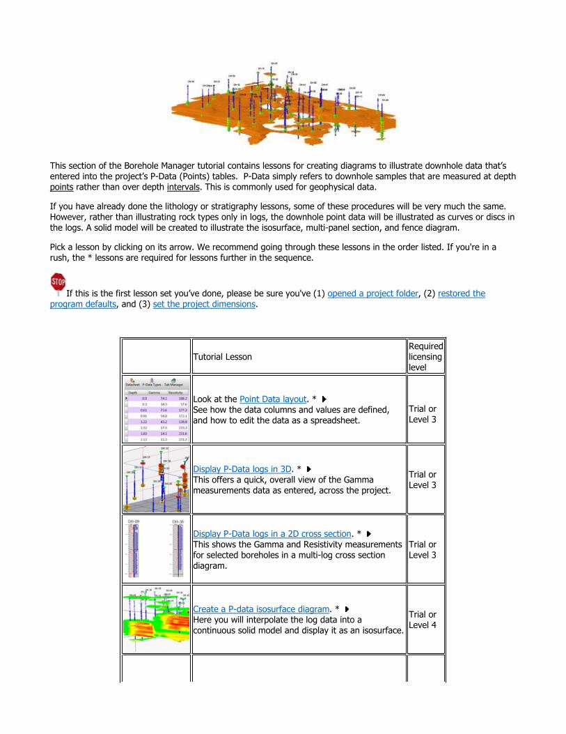
This section of the Borehole Manager tutorial contains lessons for creating diagrams to illustrate downhole data that’s entered into the project’s P-Data (Points) tables. P-Data simply refers to downhole samples that are measured at depth points rather than over depth intervals. This is commonly used for geophysical data.
If you have already done the lithology or stratigraphy lessons, some of these procedures will be very much the same. However, rather than illustrating rock types only in logs, the downhole point data will be illustrated as curves or discs in the logs. A solid model will be created to illustrate the isosurface, multi-panel section, and fence diagram.
Pick a lesson by clicking on its arrow. We recommend going through these lessons in the order listed. If you're in a rush, the * lessons are required for lessons further in the sequence.
If this is the first lesson set you’ve done, please be sure you've (1) opened a project folder, (2) restored the program defaults, and (3) set the project dimensions.
Tutorial LessonRequired licensing level
Look at the Point Data layout. * See how the data columns and values are defined, and how to edit the data as a spreadsheet.
Trial orLevel 3
Display P-Data logs in 3D. * This offers a quick, overall view of the Gamma measurements data as entered, across the project.
Trial orLevel 3
Display P-Data logs in a 2D cross section. * This shows the Gamma and Resistivity measurements for selected boreholes in a multi-log cross section diagram.
Trial orLevel 3
Create a P-data isosurface diagram. * Here you will interpolate the log data into a continuous solid model and display it as an isosurface.
Trial orLevel 4

Back to main menu
RockWare home page
Tutorial: View the Point Data Layout
Estimated time: 3 minutes.
In this lesson, you will look at how downhole "Point" data is entered, how the columns are defined, how to edit the data as a "datasheet", and how to query the data based on p-data value ranges.
1. Be sure the "Samples" folder is still the current project folder (see Open a Project for information).
2. In the borehole file listing along the left side of the Borehole Manager, click on the borehole named DH-02 to make it active.
3. Click on the P-Data (Points) button to view the table.
Create a P-data multi-panel cross section. Using the interpolated model, you'll display connected slices in a cross section diagram.
Trial orLevel 4
Create a P-data fence diagram. Using the interpolated model, you'll display multiple panels in a 3D fence diagram.
Trial orLevel 4

! Note how each row contains a single depth, and multiple columns of measurements. These values can represent gamma, resistivity, other elog data, drilling rate, or any point-sampled downhole data. (What RockWorks calls "interval" data – previous lesson set – is entered with a top and bottom depth, and measurement(s) for the interval.) If a component has no measurement for a particular depth, it can be left blank.
4. Click on the borehole DH-04 in the list to the left, and you’ll see the information listed in the P-Data table for this hole.
There's no limit to the number of components for which you can enter measurements. Let's take a look.
5. Look at the project's P-Data Types: a. With the P-Data table visible (for any borehole) click on the P-Data Types button that is displayed above
the data. The program will display the current P-Data setup.
This defines for each component type its name and its min and max values. You can also enter comments regarding units and descriptive notes. The Order value determines the column order in the Borehole Manager display, and the Visible checkbox defines whether the column is visible or not.
In your own work you can add components to the P-Data table (and columns to the Borehole Manager display) by clicking in the last shown row, pressing the down-arrow key, and defining these fields for the new measurement type.
c. Click on the Close button to close the Point (P-Data) Columns window.
6. Edit Data as Datasheet: Note that even though the data displayed in the P-Data table looks like a spreadsheet, it is not. It's actually a complicated merging of many records stored in the Borehole Manager's Point Data and Point Data Type tables. Because of this, you cannot select a block of cells like you can within a spreadsheet-type display, or copy/paste blocks of cells.There is, however, a nifty tool in the Edit menu that makes editing this data quite easy.
a. Click on the Datasheet button at the top of any of the boreholes' P-Data listings (or select the Edit | Edit Data as Datasheet option).

b. The program will load the contents of the current P-Data table for the current borehole into a true row-and-column datasheet window. Here you can select blocks of cells, copy and paste from other applications, etc.
c. Close this window by clicking the Cancel button, and respond Yes to the Cancel-all-changes prompt.
Entering P-Data
Back to P-Data menu | Next (3D logs)
RockWare home page
Tutorial: Display P-Data Logs in 3D
Estimated time: 4 minutes.
In this lesson, you will get a quick view of one P-Data component (Gamma) as entered for the project’s boreholes, by generating 3D logs.
1. To create the 3D logs, click on the Striplogs menu, and then click on 3-Dimensional | Multiple Logs.
This window has several sections:The left side is where general diagram settings are established.The 3D Striplog Designer tab is where you establish the log-specific settings.
2. Establish the general diagram settings in the left pane. Group Title: This can be left at: Logs
Clip: Uncheck this.
Reference Cage: Uncheck.
Include Lithology Legend: Uncheck.
Include Stratigraphy Legend: Uncheck.
Include Well Construction Legend: Uncheck.
3. Click on the 3D Striplog Designer tab.
The left pane is where you choose what type of data is to be displayed in the logs (the Visible Items). The upper-right pane is where you see a plan-view Preview of the active log items. You can drag the items to adjust their relative placement. The lower-right pane displays specific Options for the Visible Item that you click on.
Choose the items you want to see in the logs by inserting a check-mark in the following items in the Visible Items section of the window:
Title: The drill hole name will plot above the logs. Axis: The logs' axes will be shown with a solid line. P-Data #1: The logs will contain a column illustrating point-data values. You can include up to 4
different P-Data "tracks"; we'll display only one in this lesson.When this column is selected, you'll see a green circle displayed in the plan-view Preview pane.

Track: At the top of the Options pane, click on the Track heading and choose Gamma as the data to be represented in the logs. Column Title: This should be blank. If text is displayed for this prompt, click on this heading and delete the text. Offset Distance: Adjust the placement of the column relative to the axis of the log by dragging the circle in the Preview pane. Be sure the P-Data circle is on the center of the log axis.! You can simply type 0.0 into the Offset Distance prompt, if you prefer. Column Radius: Adjust the size of the column by dragging on one of the corner handles. Note the Column Radius setting in the lower-right Options pane. As you resize the circle, the Radius setting will be updated. Drag the P-Data #1 circle until the Column Radius is about 1.0.! You can simply type 1.0 into the Column Radius prompt, if you prefer. Scaling: Expand this heading and set the scaling to Automatic.
Plot Line: Uncheck this. Discs: Check this option to represent the data as 3D discs. Expand this heading and set the
Color Options to Cold ->Hot. None of the other Visible Items should be checked.
4. Click Process at the bottom of the Multiple Log 3D Plotting Options window to proceed.
The program will create a log for each enabled borehole, including well name at the top, and color-coded Gamma-value discs displayed down the log. They will be displayed in a new, RockPlot3D tab, to the right.
The image is displayed in the pane to the right, and the image components as well as the standard reference items are listed in the pane just to the left of the image. The expandable/collapsible list on the left is called the "data tree."
5. Adjust the reference items: a. World Outline: Check this option, if necessary, and expand this heading. b. Set the following items to be on/off:
Top: Uncheck this if necessary so that you can look down onto the log display with no interference from panels.
Base: Check this. West: Check this North: Check this
East: Uncheck this
South: Uncheck this c. Double-click on the North option.
Fill / Enabled: Check this, and select light gray for the color. Drag the Transparency slider bar to the middle. Set the Rows and Columns to 5 and the line color to red. Click OK to close the window.
d. You can continue to modify the World Outline panels as you wish. For example, you could un-check the South and East panels, and set the North and Bottom panels to the same fill and row/column settings as the North panel, above.
e. Be sure the Axes and Labels are both turned on.
6. Zoom into the scene by selecting the "200%" option from the zoom drop-down at the top of the plot window.
7. Re-adjust the rotation if you wish, even when zoomed in. Use the Pan tool to move the current view back
and forth, up and down. To zoom back out, just click once on the Zoom Out button
8. Turn on/off logs: Expand the Logs group in the data tree, to see the individual boring names. You can turn
entire logs on and off simply by checking/clearing their respective check-boxes. Try this for a few borings.
9. Turn on/off log items: In addition, if you expand an individual borehole in the data list, you’ll see its title, axis, and P-Data#1 item. These, also, can be turned on and off individually for each well.
10. Save this 3D log data: Select the File | Save As command. In the displayed window, type in this name: p-data logs and click the Save button. RockPlot3D will save this information on disk under that name, with an ".Rw3D" file name extension. In later lessons, you can append these logs to other 3D diagrams.
11. Close the RockPlot3D window by clicking in the Windows Close button .
3D Logs
Back to P-Data menu | Next (2D log section)
RockWare home page
Tutorial: Display Multiple Geophysical Logs in a 2D Cross-Section
Estimated time: 4 minutes.
In this lesson, you will be creating an image representing the Gamma and Resistivity measurements as curves in multiple logs in the Samples project, selected along a multi-log cross section trace.
1. Click on the Striplogs menu, and then click on 2-Dimensional | Section. (What's the difference between "profiles," "sections," and "projected sections"? Click here.)
2. Establish the section options: (These are found in the left pane of the Hole-to-Hole Log Section window.) Plot Striplogs: Check this
Borehole Spacing: Expand this heading to confirm that this is set to Distance between Collar Locations.
Plot Correlations: Uncheck this
Hang Section on Datum: Uncheck this.
or Plot Surface Profile: If you completed the borehole map section of the tutorial (jump back), insert a check in the Plot Surface Profile option. This is used to display a selected surface in the cross section plot. If you DID NOT complete that lesson, leave this un-checked.
Grid Model: Click here and select the GRD file representing the ground surface, named surface.RwGrd and click the Open button. Line Type: Click here to set the line style to red, medium thickness. Smoothing can be set to 1.
Plot Fault(s): Uncheck. Perimeter Annotation Options: These options determine text and lines that will plot around the perimeter of the profile. Click on this button to view the options; the factory defaults should be fine. See Restore Default Settings if you need more information about setting the factory defaults.! In your own work the Intended Vertical Exaggeration Factor can be very helpful for good diagram proportions if you have a large, flat study area and will stretch your cross sections for readability.

Create Location Map: Check this item. This will create a small map that shows the location of the profile "cut" in the study area. Expand this heading to change:
Append Map to Profiles and Sections: Uncheck this. Display Map as Separate Diagram: Check this option.
Legends: Uncheck all legends.
Clip Diagram: Uncheck this item.
3. Establish the striplog options: Now you need to set up how the logs within the cross section will look. Click on the 2D Striplog Designer tab, to the right.
The program will display the 2D log designer window. This window has three main sections: The left pane is where you choose what type of data is to be displayed in the logs (the Visible Items). The upper-right pane is where you see a Preview of the active log items. You can drag the items to adjust their relative placement. The lower-right pane displays specific Options for the Visible Item that you click on.
a. Visible Items: Choose the items you want to see in the logs by inserting a check-mark in the following items in the Visible Items section of the window:
Title: The drill hole name will plot above the logs. Depths: The logs will be labeled with depth tick marks and labels. P-Data #1: The logs will contain a column illustrating P-data values as a curve down the log. P-Data #2: The logs will contain a second column illustrating P-data values as a curve. You can
activate up to 4 P-Data columns. None of the other options, including Text, should be checked.
b. Arrangement: Adjust the arrangement of the visible log items. You should see four items in the upper Preview pane: title, depth bar, log axis, and two P-data columns.
Practice clicking on an item, holding down the mouse button, and dragging it to the left or right in the preview. Try getting the items aligned in the following order:

! Note that the log axis is always activated. It acts as the "anchor" point for the log - it's the axis that will be placed at the actual log location in the cross section diagrams. The log title is always placed atop the axis.
c. Options: Review the options for each visible item by clicking on the item's name in the listing; its options will be displayed in the Options pane.
Click on the Title item at the top of the list. You'll see Title Options displayed below and to the right. Font: Click here and set the Size to Medium, and click OK.
Click on the P-Data #1 item. Track: Click here as necessary to set the data column to Gamma. Width: Click on this item, and set it to 1. ! All log item sizes are expressed as a percent of the dimensions of the project, so the width of these logs will be about 1% of the project dimensions. Column Title: Click on this option in the right-hand pane and delete any text that's displayed there.
Background Subdivisions: Be sure this is checked, and expand this heading. Intervals: 5Plotting Sequence: Background
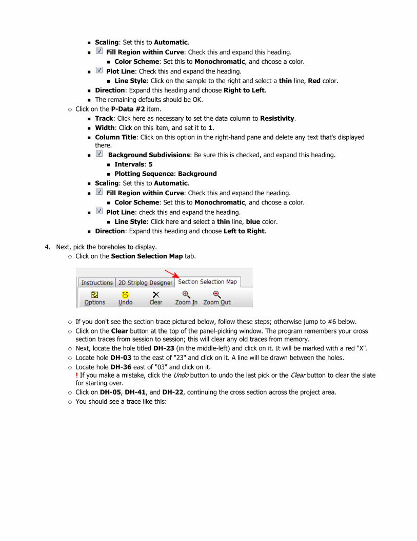
Scaling: Set this to Automatic. Fill Region within Curve: Check this and expand this heading.
Color Scheme: Set this to Monochromatic, and choose a color. Plot Line: Check this and expand the heading.
Line Style: Click on the sample to the right and select a thin line, Red color. Direction: Expand this heading and choose Right to Left. The remaining defaults should be OK.
Click on the P-Data #2 item. Track: Click here as necessary to set the data column to Resistivity. Width: Click on this item, and set it to 1. Column Title: Click on this option in the right-hand pane and delete any text that's displayed there.
Background Subdivisions: Be sure this is checked, and expand this heading. Intervals: 5Plotting Sequence: Background
Scaling: Set this to Automatic. Fill Region within Curve: Check this and expand the heading.
Color Scheme: Set this to Monochromatic, and choose a color. Plot Line: check this and expand the heading.
Line Style: Click here and select a thin line, blue color. Direction: Expand this heading and choose Left to Right.
4. Next, pick the boreholes to display. Click on the Section Selection Map tab.
If you don't see the section trace pictured below, follow these steps; otherwise jump to #6 below. Click on the Clear button at the top of the panel-picking window. The program remembers your cross section traces from session to session; this will clear any old traces from memory. Next, locate the hole titled DH-23 (in the middle-left) and click on it. It will be marked with a red "X". Locate hole DH-03 to the east of "23" and click on it. A line will be drawn between the holes. Locate hole DH-36 east of "03" and click on it.! If you make a mistake, click the Undo button to undo the last pick or the Clear button to clear the slate for starting over. Click on DH-05, DH-41, and DH-22, continuing the cross section across the project area. You should see a trace like this:

5. Click the Process button at the bottom of the Hole to Hole Section window to proceed.
The program will create strip logs of each of the selected borings using the selected settings. The logs will be spaced proportionally to their distance from each other on the ground. The completed cross section will be displayed in a RockPlot2D tab, where 2-dimensional ("flat") maps and other diagrams are presented.
In addition, it will create a map that displays the location of the section slice within the study area. The completed map will be displayed in a second RockPlot2D tab.
6. Enlarge the display area by hiding the left-hand options pane - click on the small "-" button in the middle of the divider bar.
For reference, when you want to access the options again, you can click on the same, small button, now shaped like "+".
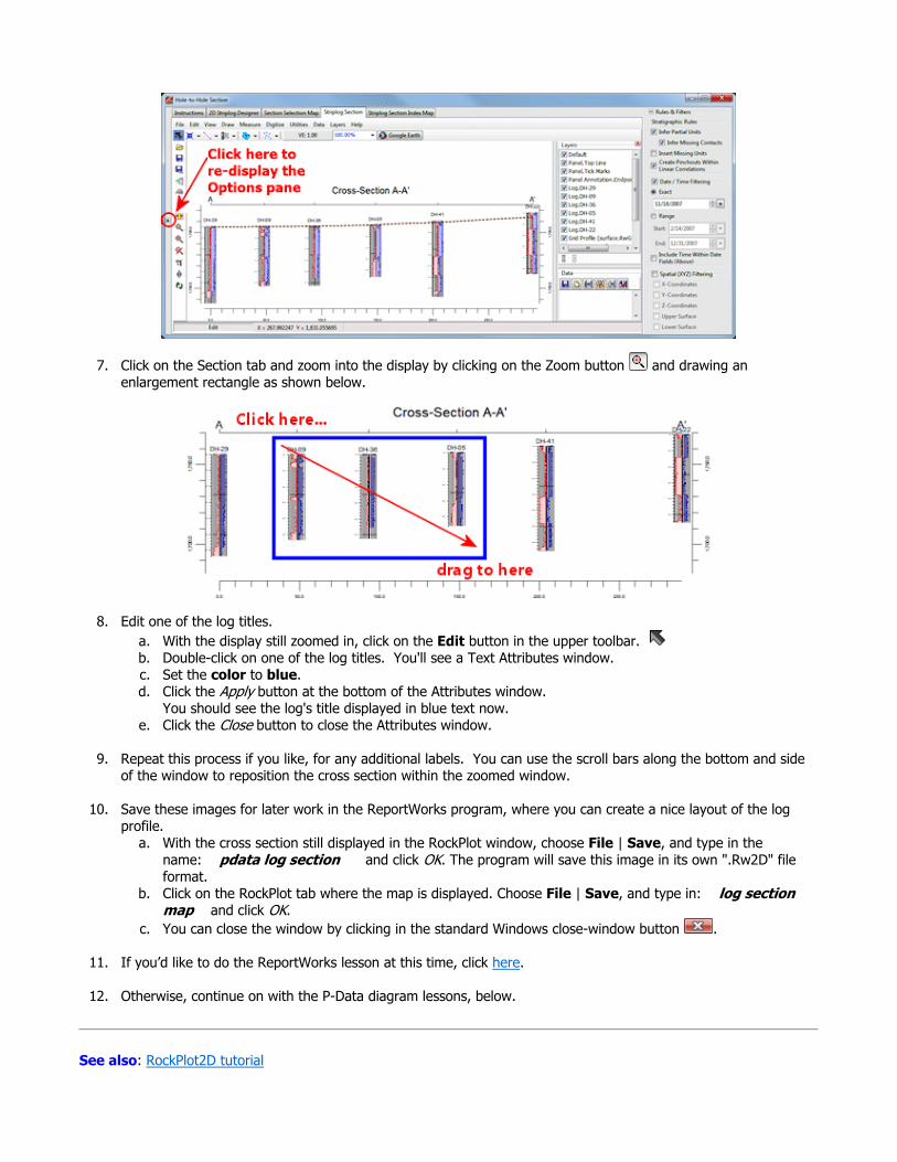
7. Click on the Section tab and zoom into the display by clicking on the Zoom button and drawing an enlargement rectangle as shown below.
8. Edit one of the log titles. a. With the display still zoomed in, click on the Edit button in the upper toolbar. b. Double-click on one of the log titles. You'll see a Text Attributes window. c. Set the color to blue. d. Click the Apply button at the bottom of the Attributes window.
You should see the log's title displayed in blue text now. e. Click the Close button to close the Attributes window.
9. Repeat this process if you like, for any additional labels. You can use the scroll bars along the bottom and side of the window to reposition the cross section within the zoomed window.
10. Save these images for later work in the ReportWorks program, where you can create a nice layout of the log profile.
a. With the cross section still displayed in the RockPlot window, choose File | Save, and type in the name: pdata log section and click OK. The program will save this image in its own ".Rw2D" file format.
b. Click on the RockPlot tab where the map is displayed. Choose File | Save, and type in: log section map and click OK.
c. You can close the window by clicking in the standard Windows close-window button .
11. If you’d like to do the ReportWorks lesson at this time, click here.
12. Otherwise, continue on with the P-Data diagram lessons, below.
See also: RockPlot2D tutorial

Displaying Multiple Logs in a 2D Hole to Hole Section
Back to P-Data menu | Next (model & isosurface)
RockWare home page
Tutorial: Create a P-Data Model and Isosurface Diagram
Estimated time: 4 minutes.
Now we will jump from the Striplogs menu, where we plotted observed data in log diagrams, to the P-Data menu, where the downhole quantitative data will be interpolated into a continuous model.
In this lesson, you will create a solid model and 3-dimensional isosurface diagram of the project's Gamma measurements. The program will load the recorded borehole data, that you viewed in logs and log sections already, and extrapolate the gamma values throughout the project. This modeling process basically "fills in the blanks" between the logs. RockWorks offers several modeling algorithm to do this extrapolation.
! You must be using RockWorks in Trial mode, or have a Level 4 or 5 license to run this modeling program.
Before continuing, be sure you have opened the sample project, established the project dimensions and created 3D logs, as discussed in earlier lessons.
1. Back at the Borehole Manager, click on the P-Data menu and select the Model option.
2. Establish the modeling settings: Create New Model: Click in this button, and expand this item. This tells RockWorks that we want to
interpolate a new solid model file. P-Data Track: Click here to select from the pop-up list the column titled Gamma. Expand this heading and be sure that none of the data filters are turned on. Solid Model Name: Click here and type in: gammaThis will be the name assigned to the solid model to be created, with an ".RwMod" file name extension. Solid Modeling Options: Click this button to access the various modeling settings.
Algorithms: These options determine the method that will be used to interpolate the P-Data model. Click in the IDW Anisotropic radio button to select this Inverse-Distance Anisotropic modeling method. Additional Options - Turn the following items on/off. Note that you can click on any of these tabs to read more information.
Dimensions: These define the extents of the output model. Based on Output Dimensions: Be sure this option is checked.
Confirm Model Dimensions item can be left unchecked (though in your own work, this is a handy way to double-check the model extents and node spacing).
Add Points: unchecked. Decluster: Checked.
Cutoff - H, Cutoff - V: unchecked.
Logarithmic: unchecked. Smoothing: Checked.
HiFi: unchecked.
Distance: unchecked.
Polygon: unchecked. Superface: Check this to activate an upper surface (grid) filter, and click on the tab to
access the settings. Choose Automatic. RockWorks will automatically determine a surface

representing the ground and filter out (nullify) nodes that sit above that surface. Buffer Size: Set this to 0.
Subface: Check this option to activate a lower surface filter, and choose Automatic to filter nodes below the borehole bases. Buffer Size: Set this to 0.
Tilting: unchecked. If activated, this can be used to apply a tilt to the model.
Warping: unchecked. If activated, this can be used to warp a model based on a surface.
Faulted: unchecked. If activated, you can use a 3D "fault file" to introduce faults into your model.
G=Color: unchecked. This is used for color modeling only. Undefined: Click here to select Null for undefined/filtered nodes. In this case, nodes which lie above the ground surface or below the borehole bases will be set to the RockWare null value (-1e27); they will be invisible in display and will not contribute to volume computations, etc.
Click OK to close this window.
3. Create 3D Diagram: Check this, and expand this heading to access the diagram settings. Diagram Type:
Isosurface: This will create a diagram in which the different G value levels can be represented as if enclosed within a "skin" that is like a 3-dimensional contour. Within RockPlot3D you will be able to interactively adjust the minimum P-data value to be enclosed within the isosurface contour.
Iso-Mesh: Uncheck this. Plot Logs: Check this. The program will generate the 3D logs using the same settings we used in an
earlier lesson in this section. Reference Cage: Check this. Expand this heading and click the Cage Options button.
Dimensions: This should be set to the Automatic.
Panels: Be sure these are all unchecked. (Click the All Panels: Off button to disable all.)
Grids: These should also be unchecked. Axis Labels: Check these options only; you can refer to the cartoon for a preview.
SouthwestBase / WestBase / South
Color Scheme: You can click on this Options button to choose a color scheme that you like for the isosurface display. For example, for cold-to-hot gradational colors, choose the upper (2-Colors) option and click on the long color bar to choose the gradational scheme. Or, just click on the left and right color boxes below the long bar, to choose the colors which will represent the minimum and maximum values in the model.
Include Color Legend: Insert a check-mark here.
4. Click the Process button at the bottom of the P-Data Model window. RockWorks will create two items:
It will interpolate a solid model at the specified project dimensions usng the Inverse-Distance Anisotropic modeling method. The model will stored in the project folder under the name "gamma.RwMod"
Once the model is completed RockWorks will create an isosurface diagram to represent the model, with the full range of values displayed. The completed diagram will be displayed in a RockPlot3D tab.
5. View the isosurface model options by double-clicking on the Gamma item that’s listed in the data tree. (You can also right-click on the Gamma item and choose Options.)

The program will display a window listing the Isosurface Options. Here’s a quick summary:
Color scheme: Unlike the lithology model you may have created in an earlier tutorial, this solid model contains "G" values representing gamma measurements that range from a minimum to a maximum. The default scheme will be set to Continuous, to show gradations between the low and high values. . Draw Style: Default is Solid. You might try changing the display to Wire Frame to see the effect. Click the Apply button at the bottom of the window to make any changes you set take effect. Using Wire Frame can speed rendering of the solid if it is dense or your computer system is slow. Opacity: You’ll see this one in most 3D Options windows. You can make the block more transparent by reducing the percent opacity shown here. Again, use Apply to see changes take effect. Cap Style: This tells the program how you want the "blobs" that intersect the edge of the model to be displayed. By changing the contour interval, you can see how the concentrations change inside the isosurface. Iso-level: This allows you to see only selected G values in the block. See #8 below. Slices: This allows you to see insert horizontal or vertical slices at specific locations in the block.
If you have a minute, you should go through the next few steps to learn some of the ins and outs of viewing isosurface diagrams. If you are in a hurry, you can review these lessons later in the dedicated RockPlot3D tutorial.
7. Adjust the View: Leave the Isosurface Options window open while you Rotate or Pan the image pane display. (You have full control over the image display even when one or more Options windows are open.) Or, use the View | Above or Below or Compass Points tools to return to a pre-set view.
You can save one or more views for quick access later, using the View | Add View option.
8. Change the iso-level being displayed: Click back in the Isosurface Options window, and find the slider bar in the Iso-Level section. The left-hand value on this slider corresponds to the minimum gamma readings, and the right-hand value represents the maximum.
a. Drag the slider bar slowly to the right, with the intention of changing the minimum gamma level displayed, to see how the display changes. In your own work you can use the slider or just type a minimum desired value into the prompt.Remember, you can rotate and pan the image at any time without closing the Options window to get a better view.
b. Set the Iso-Level to 50 by typing that value into the Iso-Level Value prompt and clicking the Applybutton. The solid model representation will now display only those gamma values greater than or equal to 50.
9. Insert some slices: a. Now, click in the North-South button in the Slices section at the bottom of the Options window. This

tells the program that you want to insert a vertical slice from south to north in the model. The slider bar will show the western project coordinate to the left and the eastern project coordinate to the right.
b. Move the slider bar to the middle, and click Add.The program will insert a north-south slice in the model, at the Easting coordinate shown above the slider, and it will insert a slice entity in the Data listing in the data pane.
c. Drag the slider bar to the right and click Add. The program will insert a slice along the eastern boundary of the model, and a new item will be listed in the Data pane.
d. Repeat this process if you would like to insert vertical East-West slices. For these entities, the slider bar will represent southern coordinates to the left and northern coordinates to the right.
e. If you want to remove a slice, right-click on the slice’s name in the data pane, and choose Delete from the pop-up menu.
f. If you want to hide the isosurface (blob) to view all of the slices, set the Draw Style to Hidden.
10. Close the Isosurface Options window by clicking the Close button.
11. Adjust a slice: a. Double-click on one of the slices you had inserted into the model. You will see the Slice Options window. b. Locate the Position slider bar at the bottom of the Options window. Watch what happens as you drag
the slider – the position of the slice in the view window will change as you drag the slider from left to right. The north-south or east-west coordinate (vertical slices) or elevation (horizontal slices) will be shown at the top of the tab as you drag. The slice’s coloration will vary as it moves through the solid model.
c. Close the Slice Options window when you are ready to continue.
12. If you want to save this view, choose File | Save and enter: gamma_solid and click Save.
13. Close this RockPlot3D window by clicking in its upper-right Close box .
Solid Modeling Reference, Creating P-Data Models
Back to P-Data menu | Next (interpolated cross section)
RockWare home page
Tutorial: Create a Modeled P-Data Cross Section
Estimated time: 3 minutes.
In this lesson, you will create a multi-paneled set of section panels using the P-data model you created in the previous lesson. The instructions below are written with the assumption that you have completed the previous lesson, as well as the lesson on log sections.
1. Click on the P-Data menu and choose Section.
2. Establish the modeling settings:Use Existing Model: Since you took the time to create a solid model in the previous lesson, we can use
that one for this tutorial. Expand this item. Model Name: Click here to browse for the file "gamma.RwMod".
! This is important to remember in your own work. Once a solid, numerical model is created to represent your data, and saved on disk as an .RwMod file, you can use that same model to create different types of diagrams – profiles, sections, fences, isosurfaces, slices – without having to recreate the solid model each time.
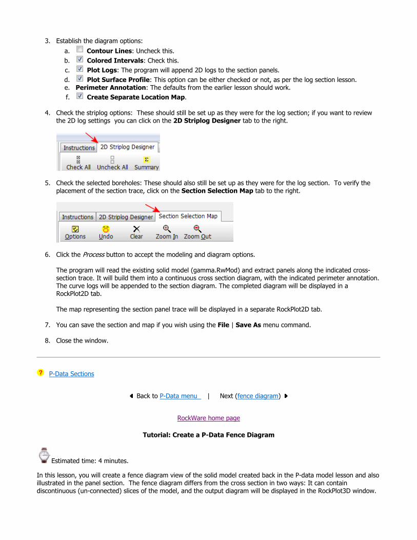
3. Establish the diagram options: a. Contour Lines: Uncheck this. b. Colored Intervals: Check this. c. Plot Logs: The program will append 2D logs to the section panels. d. Plot Surface Profile: This option can be either checked or not, as per the log section lesson. e. Perimeter Annotation: The defaults from the earlier lesson should work. f. Create Separate Location Map.
4. Check the striplog options: These should still be set up as they were for the log section; if you want to review the 2D log settings you can click on the 2D Striplog Designer tab to the right.
5. Check the selected boreholes: These should also still be set up as they were for the log section. To verify the placement of the section trace, click on the Section Selection Map tab to the right.
6. Click the Process button to accept the modeling and diagram options.
The program will read the existing solid model (gamma.RwMod) and extract panels along the indicated cross-section trace. It will build them into a continuous cross section diagram, with the indicated perimeter annotation. The curve logs will be appended to the section diagram. The completed diagram will be displayed in a RockPlot2D tab.
The map representing the section panel trace will be displayed in a separate RockPlot2D tab.
7. You can save the section and map if you wish using the File | Save As menu command.
8. Close the window.
P-Data Sections
Back to P-Data menu | Next (fence diagram)
RockWare home page
Tutorial: Create a P-Data Fence Diagram
Estimated time: 4 minutes.
In this lesson, you will create a fence diagram view of the solid model created back in the P-data model lesson and also illustrated in the panel section. The fence diagram differs from the cross section in two ways: It can contain discontinuous (un-connected) slices of the model, and the output diagram will be displayed in the RockPlot3D window.

The instructions below are written with the assumption that you have completed the 3D Logs and P-data modellessons.
1. Back at the Borehole Manager, click on the P-Data menu and select the Fence option.
2. Establish the modeling settings:Use Existing Model: Again, you've already created the model that represents the P-Data, and you can use
that model for the fence diagram display. Expand this item.Model Name: Click here to browse for the file "gamma.RwMod".
3. Establish the diagram options: a. Color Scheme: Click on the Options button to select the desired color scheme for the fence panels. b. Include Color Legend: Check this.
c. Plot Outline Around Each Panel: Uncheck this. d. Plot Surface Profile: Uncheck this. e. Plot Logs: The program will append 3D logs to the 3D view, using the same settings we used in an
earlier lesson in this section. f. Reference Cage: Uncheck this. g. Create Separate Location Map. Check this, to display your fence panel arrangement in plan-view.
4. Click on the 3D Striplog Designer tab if you'd like to review the striplog setup.
5. Click on the Fence Selection Map next, to define the layout of the fence panels.
Unlike profile diagrams, fence diagrams permit multiple panels to be selected. These can be drawn in several ways:
Interactively by you, by clicking the beginning and ending points of the panels, just like you drew the cross section slices, and/or Using pre-set panel selections, offered in the buttons to the left, and/or From coordinates listed in an "X Y Pairs" table in the database.
For this tutorial, we will use the second option.
6. Select the Fence Panels: If the fence panel layout doesn't look like that which is shown below, continue with these steps. Otherwise, jump to #7.
a. Clear: Click on the Clear button at the top, to remove any existing panels.
b. Snap: Clear this box (upper-left). This allows the panels to be drawn anywhere within the model, not just between boreholes.
c. Click on the N & S button, to the left. The program will draw horizontal lines along the north and south borders of the project.
d. Click on the E & W button. You will see vertical lines drawn along the western and eastern borders of the project.
e. Click on the Cross button. The program will add north-south and east-west panel lines to the map window.

In your own work, you can use any combination of hand-drawn and/or pre-set panel configurations. If you wish to erase the current panels to re-draw, simply click the Clear button to clear the display.! Because the P-Data model is continuous, you can place the fence panels anywhere within the model - you don't have to place the panel endpoints at the borehole locations.
7. Click the Process button at the bottom of the P-Data Fence Diagram window to continue.
The program will read the contents of the existing gamma solid model file and will create vertical slices through the model along the indicated panel lines. The completed diagram will be displayed in a RockPlot3D tan. Three-dimensional logs will be appended to the fence diagram.
Note: The image is displayed in the pane to the right, and the image components as well as the standard reference items are listed in the pane to the left of the image.
8. Expand the Gamma Fence item in the Data listing. Note that the 6 vertical panels are listed there. Each can be expanded, where the panel outline and vertical grid model are listed. (If you can’t tell which panel name corresponds to which panel in the view, remove a check-mark and see which one disappears.)
9. Adjust the display as you wish using the Rotate and Pan buttons.
10. Adjust the panel opacity: You can adjust the opacity of an entire group of objects (such as the fence panels) by double-clicking on the Gamma Fence item (the heading with the icon) . Set the Opacity setting to 70 and click Apply. This will apply the new setting to all of the items below this group heading. You should now see the logs better. Close the transparency window.
11. Turn data items on and off: Take a moment to experiment with turning display items on and off, using the check-boxes in the Data listing in the data pane.
12. Save this image: Select the File | Save command. In the displayed window, type in this name: pdata logs+fence and click the Save button. RockPlot3D will save this combined information on disk under that name, with the ".Rw3D" file name extension.
13. Close this plot window by clicking in the Windows Close button in the upper-right corner.
This is the end of the tutorial for point-based data. For more information about the RockPlot3D display window, visit that tutorial.
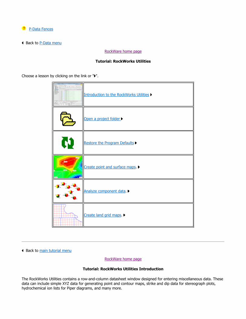
P-Data Fences
Back to P-Data menu
RockWare home page
Tutorial: RockWorks Utilities
Choose a lesson by clicking on the link or " ".
Back to main tutorial menu
RockWare home page
Tutorial: RockWorks Utilities Introduction
The RockWorks Utilities contains a row-and-column datasheet window designed for entering miscellaneous data. These data can include simple XYZ data for generating point and contour maps, strike and dip data for stereograph plots, hydrochemical ion lists for Piper diagrams, and many more.
Introduction to the RockWorks Utilities
Open a project folder
Restore the Program Defaults
Create point and surface maps.
Analyze component data.
Create land grid maps.

The Utilities datasheet is accessed by clicking on the "Utilities" tab along the top edge of the program window.
This data window has its own suite of menu options. The data you enter into the Utilities datasheet can be used to create many different types of maps and diagrams.
"Borehole" data, consisting of downhole lithology, stratigraphy, geochemistry, geophysical and other measurements are entered into the separate "Borehole Manager", discussed in a separate section of this tutorial (click here to jump to that lesson set). The Borehole Manager tools are not available if you purchased the Utilities portion of the program only (RockWorks Level 2).
Back to main menu | Next (Open project)
RockWare home page
Tutorial: Restore the Program Defaults
The purpose of this step is to reset all of the project-specific menu settings to their factory defaults. This will eliminate the need to establish dozens and dozens of settings as you go through the tutorial.
!!! NOTE !!! This will set all of the menu options to the RockWare defaults, for this Samples project folder only. This means that if you have done a lot of work within the program, and have tweaked a lot of the menu items as you worked with the Samples data, these settings will be lost. If this is a worry for you, you might consider the following: Before restoring the factory defaults, you can use the Preferences | Export Menu Settings option to store all of your current settings in a file that can later be imported back into the program using the Preferences | Import Menu Settings option.
Step-by-Step Summary
1. If you have just installed RockWorks you can skip this step because program defaults have already been established. (Click the Next button below.)
2. If you’ve been running RockWorks for a while (or if you aren’t sure), you should click on the Preferences menu and choose Reset Menu Settings.
3. Establish these menu options: Reset Global Settings: Uncheck this item. Reset Project Settings: Check this item. It will reset the project-specific settings to factory
defaults. 4. Click on the Process button at the bottom of the window.
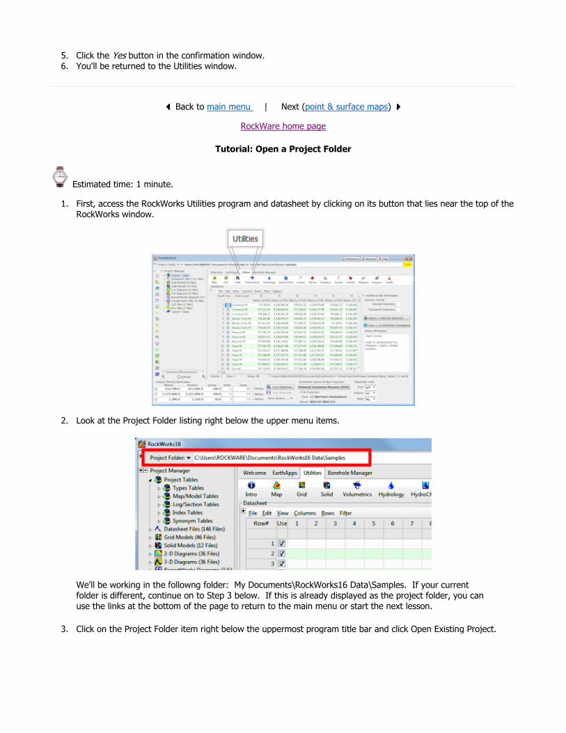
5. Click the Yes button in the confirmation window. 6. You'll be returned to the Utilities window.
Back to main menu | Next (point & surface maps)
RockWare home page
Tutorial: Open a Project Folder
Estimated time: 1 minute.
1. First, access the RockWorks Utilities program and datasheet by clicking on its button that lies near the top of the RockWorks window.
2. Look at the Project Folder listing right below the upper menu items.
We'll be working in the followng folder: My Documents\RockWorks16 Data\Samples. If your current folder is different, continue on to Step 3 below. If this is already displayed as the project folder, you can use the links at the bottom of the page to return to the main menu or start the next lesson.
3. Click on the Project Folder item right below the uppermost program title bar and click Open Existing Project.

4. In the displayed window, browse to the tutorial project folder we’ll be working with: First open the "RockWorks16 Data" folder (in "My Documents") and the "Samples" which is inside of that. When the Samples folder name is highlighted, click the Select button to select it.
You will be returned to the main data window, with that folder displayed as the current project folder. All of the RockWorks-related files contained in this folder will be displayed in the Project Manager pane, along the left edge of the program window.
Back to main menu | Next (restore defaults)
RockWare home page
Tutorial: Create Point and Surface Maps

These lessons will focus on the tools in the Utilities Map menu: point maps, contour maps, and 3D surface maps.
Pick a lesson by clicking on its its link or arrow ( ). We recommend going through these lessons in the order listed.
If this is the first lesson you’ve done, please be sure you’ve (1) opened a project folder and (2) restored the program defaults.
Back to main menu
Open a data file
Set the output dimensions
Create an EZ point map
Create an EZ contour map
Create a grid-based 2D contour map
Create a grid-based 3D surface

RockWare home page
Tutorial: Open an XYZ Data File
Estimated time: 1 minute.
1. Access the RockWorks Utilities datasheet and open the Samples project folder, as described earlier. (Remind me… )
2. Locate the Project Manager pane along the left edge of the program window. Here you'll see groupings of a variety of different RockWorks file types in the Samples folder.
3. Expand the Datasheet Files heading in the Project Manager. You'll see a long list of sample data files.
4. Locate the file "Soil_Properties_01.RwDat" at the bottom of this listing, and double-click on it. The program will load the contents of the data file into the Utilities datasheet.
This particular file contains borehole IDs, symbols, X (easting) and Y (northing) location coordinates, surface elevation at those sites, and a number of soil measurements. This is a basic "XYZ" file that we can use for creating point maps and contour maps.
! RockWorks permits you to organize your data almost any way you like. Any time you want to create a map or diagram, you can specify which columns in the datasheet contain what type of data.
5. View the Column Parameters: Right-click in the gray column heading for the ID column (or select Columns | Column Properties). The program will display the column parameters window.

This is where you can assign the column title and column type. The ID column is a "Generic" text column.
6. Click the green arrow at the top of the window to proceed to the next column's settings.
Here you'll see that the Symbol column is set up to be a Graphic column containing "Vector Symbols". This tells RockWorks to display graphic symbols in this column.
7. Click the green arrow at the top of the window again to advance to the Easting column.
This column contains geographic coordinates. Here you can specify the coordinate type and the units.
! X and Y coordinate columns must have type and units selected for map creation. In your own work, if you don't know/don't care what your coordinates represent, just choose Local Feet or Local Meters as appropriate.

8. Click the green arrow to advance to the Northing column - it's also set as a Geographic/Spatial column, with coordinate system and units selected.
9. Advance to the next column, Elevation. This is set to a Linear (Z) Dimension column type, with units also selected.
10. Continue scrolling through the columns in this datasheet to see their setup.
11. Click OK to close the Column Settings window.
Opening an Existing Datasheet, Changing Column Titles and Styles, Using the Project Manager
Back to map menu | Next (project dimensions)
RockWare home page
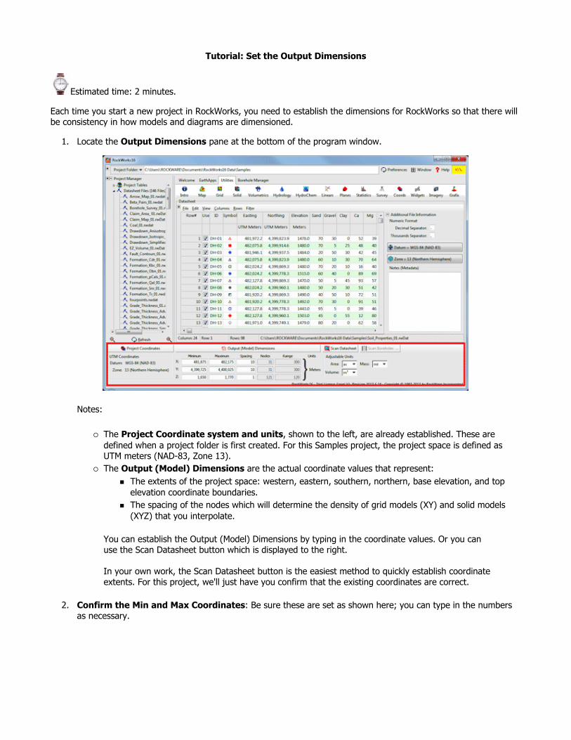
Tutorial: Set the Output Dimensions
Estimated time: 2 minutes.
Each time you start a new project in RockWorks, you need to establish the dimensions for RockWorks so that there will be consistency in how models and diagrams are dimensioned.
1. Locate the Output Dimensions pane at the bottom of the program window.
Notes:
The Project Coordinate system and units, shown to the left, are already established. These are defined when a project folder is first created. For this Samples project, the project space is defined as UTM meters (NAD-83, Zone 13). The Output (Model) Dimensions are the actual coordinate values that represent:
The extents of the project space: western, eastern, southern, northern, base elevation, and top elevation coordinate boundaries. The spacing of the nodes which will determine the density of grid models (XY) and solid models (XYZ) that you interpolate.
You can establish the Output (Model) Dimensions by typing in the coordinate values. Or you can use the Scan Datasheet button which is displayed to the right.
In your own work, the Scan Datasheet button is the easiest method to quickly establish coordinate extents. For this project, we'll just have you confirm that the existing coordinates are correct.
2. Confirm the Min and Max Coordinates: Be sure these are set as shown here; you can type in the numbers as necessary.

3. Set the Node Spacing: a. X-Spacing: Be sure this prompt is set to: 5. This means that there will be a model node placed every 5
meters from west to east across the project space. This will generate 61 nodes from west to east in the models. You’ll note that when you change the Spacing setting, the number of nodes represented will be updated automatically.
b. Y-Spacing: Type in: 5. This will generate 61 nodes from south to north in the models, also at a 5-meterspacing.
c. Z-spacing: Type in: 1. This means that the nodes will be 1 meter apart from the base of the project to the top.
! In your own work, the appropriate node spacing will depend on the spacing of your wells and downhole measurements. See How Dense is Dense Enough for some tips.
! The project dimensions settings are stored in the project database, and are loaded each time you access that project folder.
Viewing and Setting Your Project Dimensions
Back to map menu | Next (point map)
RockWare home page
Tutorial: Create a Point Map
Estimated time: 5 minutes.
If this is the first lesson you’ve done, please be sure you've (1) opened the Soil_Properties_01.RwDat data file and (2) set the output dimensions.
1. First, let's define the default font style you want to use for your 2D maps and diagrams. a. Click on the Preferences menu at the very top of the main RockWorks program window (right side).
Choose the General Program Settings menu option. b. Locate the RockPlot2D tab along the left. c. Locate the Default 2D Font item, and you'll see the current font style to the right (probably Arial). If you
would like to choose a different font, click on the current name and choose another from the pop-up list. This tells RockWorks to use the selected font for map labels, contour line labels, cross section labels, etc. Once a map or diagram is displayed, you can edit individual labels as you like.
d. You are welcome to look at some of the other program preferences you can establish here. e. Click the OK button at the bottom of the window to close the Settings window.
2. Click on the Map menu at the top of the Utilities window, and choose the EZ Map option.
3. Input Columns: In the prompts along the left side of the window, be sure the following columns are selected. This tells RockWorks which columns contain the input data. (If the wrong column title is displayed, just click on the down-arrow and scroll up or down to the correct column title.)
a. X (Easting): Easting b. Y (Northing): Northing c. Z (Elevation): Elevation
Next, set up the map layers in the next pane to the right, where there's a "tree menu" with a variety of map options. Expand and collapse headings by clicking on the small "+" or "-" buttons.
4. Symbols: Be sure this option is checked so that the map will include location symbols. Expand the Symbols heading if necessary and click on the Symbol Options button.
a. Uniform: Uncheck this. b. Column-Based: Check this option. This tells the program to use symbols stored in a column in the
datasheet to represent the map locations. Click on the Column-Based tab to see its settings. Symbol Column: Choose the datasheet column named Symbol which, as you might guess, tells the program where to read the symbols from. You may need to scroll upward to find the Symbol column name in the list. Dimensions: Choose Uniform, and enter a Size of 1.0. These dimensions represent a percent of the map width. In your own work, should you wish to increase the size of the symbols, just set the Size to a greater percentage.
c. Circles: Uncheck this. (This is sed to create scaled "bubble map" symbols.) d. Table-Based: Uncheck this. (This is used to plot specific symbols at specific colors and sizes based
on measured values.) e. Images: Uncheck this. (This is used to plot small images at the map locations.) f. Click OK to close this window.
5. Labels: Check this option to include labels with the symbols. Expand the Labels heading and click on the Labeling Options button. Here you'll see a lot of map labeling options - click the Help button if you want more complete details.
a. Plot Label: Northeast: check this. Data Column: Choose the ID column - click on the small down-arrow to see a list of the data columns. This tells the program to plot sample ID labels to the northeast of the symbols. The default text color and background color should be fine.
b. Plot Label: Southeast: Check this option. Data Column: Choose the Elevation data column. This tells the program to plot the elevations to the southeast of the symbols. As above, the default text and background colors should be fine.
c. Plot South Label, Plot Southwest Label, etc: The remaining Plot Label check-boxes should be cleared.
d. The remaining default label options should work well. (Font size and offset = 1.0, horizontal orientation with frames and leader lines.)
e. Automatic Offset: Uncheck this. (Note, though, that this is a very nifty tool to use in your own work. It prevents overplotting in crowded maps.)
f. Click OK to close this window.
6. Contour Lines: Uncheck this.
7. Color Intervals: Uncheck. 8. Decluster Points: Uncheck.
9. Network: Uncheck. 10. Background Image: Uncheck.
11. Border: Check this. The border defaults should work well, but expand this heading to click on the Border

Options button; you can look at the options that are available (axis text, etc.). a. Border Dimensions: Choose Output Dimensions. b. Click OK to close the Border Options window.
12. Click the Process button at the bottom of the EZ-Map window.
The program will create a simple point map. The datasheet symbols will be plotted at the X,Y coordinates specified for the sample sites. Each symbol will contain an ID and elevation label. The map borders will include tick-marks, coordinate labels, and titles.
The completed map will be displayed in a RockPlot2D tab, where 2-dimensional maps and diagrams are displayed. RockPlot2D contains printing, exporting, screen-digitizing and measuring tools, it allows you to combine images, and more. These are covered in the separate RockPlot2D tutorial.
13. Maximize the window (using the Windows Maximize button in the upper right corner of the window).
14. Enlarge the map window by hiding the left-hand Options pane - click on the small "-" button in the middle of the divider bar.
(For reference, you can access the Options pane again by clicking on the small "+" button along the left margin.)

15. Move the cursor around the map window, and note that the X and Y coordinates listed at the bottom of the window are updated as you move. Use this feature to view the coordinates for any point on the map.
16. Locate the Layers pane: The Layers are displayed to the right of the map. (If they are not, click on the tiny "+" button at the upper right corner of the window, to display the map Layers. Experiment with turning a layer off (by removing the check-mark) and on again.
17. Save this map : a. Click on the RockPlot2D File menu, and choose the Save option. b. In the displayed window’s File Name prompt, type in: point map and click the Save button. RockPlot
will save the map image under that name, with an ".Rw2D" file name extension.
18. Don't close the map window - we're going to make a couple of changes to the options and create a new map.
EZ Maps
Back to map menu | Next (EZ contours)
RockWare home page
Tutorial: Create an EZ Contour Map
Estimated time: 4 minutes.
Contour maps illustrate elevations or other measured data in the study area using lines or colored intervals. "Easy" contours are constructed using the same technique you would draw contours by hand, using a "Delaunay" triangulation technique. (See Creating a Grid Based Contour Map in the next lesson for another contouring method.)
! This lesson assumes that you have completed the previous lesson. We are just going to change a few settings to create a new map.
1. With the point map still displayed, return your focus to the map options in the pane on the left side of the window. (If necessary, you can re-display the Options pane by clicking on the small "+" button on the divider.)

2. Contour Lines: Insert a check here. Click on the Options button. a. Intervals
Regular: Choose regular contour intervals to get contours at regular intervals (e.g. every 5 meters).
Confirm Intervals: Check this. b. Labeling
Label Contours: Check this. The default settings should be fine. c. Color / Styles
You’ll see the default line style for labeled and unlabeled contours. You can adjust these if you like. Smoothing: Click here and type in: 1.
d. Skip...: Be sure the "Skip Zero Contour", "Skip Low Values", "Skip High Values", and "Omit Segments Near Faults" are turned off.
e. Click OK to close this window.
3. Colored Intervals: Insert a check in this check-box, and click on the Options button to access the settings. a. Scheme:
a. With 2-Colors selected, try clicking on the small color button on the left edge of the palette bar, and choose a color. Do the same for the color button on the right side - you'll see a gradation of colors
b. Another method for choosing a scheme is to click on the large color palette bar - you'll see a popup list of some pre-configured color schemes.
c. In this exercise we will just use the default Cold -> Hot (Medium) palette. This means that lower elevations will be color-filled with cold colors (purples, blues), and higher elevations with hot colors (orange, red).
b. Confirm: Insert a check in this box. c. Legend: Insert a check here, too. The default settings should work well. d. Click OK to close this window.
4. Interpolate Edge Points: This last prompt should NOT be checked. This tells the program to build contours only to the given map points, not all the way to the edge of the map area.
5. Click the Process button at the bottom of the EZ Map window to re-create the map.
Because you activated the "confirm intervals" options, the program will display a window summarizing the Z (elevation) values found in the datasheet, and some recommended labeled and unlabeled contour intervals (top)

and color-contour intervals (bottom).
6. Click OK to accept these.
The program will scan the datasheet, determine the location coordinates for each sample site, and build line contours and color-filled contour intervals to represent the surface elevations. It will overlay point symbols and labels to illustrate the control point locations, and it will annotate the border with titles, ticks, and coordinate labels. The completed map will be displayed in a new RockPlot2D tab on the screen.
Let's keep a copy of this map around while we make a grid-based contour map in the next lesson.
7. Click on the Copy to New Window button and you'll see a new, stand-alone RockPlot window, displaying the EZ Contour map.
8. Move this window to the upper-right corner of your screen or to another monitor - to move a window, just click-and-hold on the RockPlot title bar, and drag the window to a new location. Or, minimize the window if you need the space.
9. Click on the small Save button to save this map.Type in the name: ez map and click the Save button.
10. Leave this new contour map window open (we can compare it to the grid-based map in the next step).
11. Close the original EZ Map window ; you can answer No to the save-file prompt.
EZ Maps
Back to map menu | Next (grid-based contours)
RockWare home page
Tutorial: Create a Grid-Based 2D Contour Map
Estimated time: 4 minutes.
Contour maps illustrate elevations or other measured data in the study area using lines or colored intervals. "Grid-based" contours are constructed from an intermediate numeric model that the program computes for the given data points, extrapolating data into areas without control points. This model contains X,Y,Z values in a regularly spaced grid (hence its name, "grid model") which can serve as the basis for 2D and 3D contour maps, for volumetric computations, and more.
! This lesson assumes that you have completed the previous lesson before continuing. All of the mapping settings will be the same as those used in that lesson.
1. With the Soil_Properties_01.RwDat file still displayed in the datasheet, select the Map | Grid-Based Map menu command.
2. Input Columns: The prompts along the left side of the window should still read the following (from the previous lesson); if the wrong column title is displayed, just click on the down-arrow and scroll up or down to the correct column title.
a. X (Easting): Easting b. Y (Northing): Northing c. Z (Elevation): Elevation d. The Dip Gridding input will be ignored since we won't be using this method.
3. Direction Represents: These settings are only used if the Dip Gridding method is selected; you can ignore
these at this time.
4. Data Source: Choose Datasheet. (In your own work, if you want to create a grid model from a huge list of XYZ points, you can bypass the loading of the points in the Utilities datasheet by reading directly from the external ASCII file.)
5. Grid Model: This heading contains important settings for how the program will interpolate the elevations in the grid model.
Create New Grid: Select this option, to tell RockWorks that you want to interpolate a new grid model for the soil data. Expand this heading.
a. Grid Name: Click to the right to type in a name for the grid model which will be created: elevationsRockWorks will append the ".RwGrd" file name extension automatically.
b. Gridding Options: Click this button. Algorithms: These options determine the method that will be used to interpolate the grid model.
Triangulation: Click in this radio button. Interpolate Edge Points: Click in this radio button. This tells the program to
compute grid node values outside the control points (as opposed to assigning them a constant value). Refer to the links below for more information about gridding.
! Note that the options which are visible will change if you choose a different gridding method.
Grid Dimensions: Based on Output Dimensions: This should be the default setting. The surfaces will be
dimensioned as per the settings under the Output Dimensions. If you’d like to double-check these settings, you can click the Adjust/Examine Output Dimensions button to view the window you saw back in the Set Output Dimensions lesson.! In your own work, we recommend you choose this option so that the grid and solid model dimensions are consistent. However, the program does offer the option to vary the model dimensions, under the Variable Dimensions heading.
Confirm Grid Dimensions: Check this. The program will display a summary window prior to creating the model.
Additional Options: Set these options. Decluster: On
Logarithmic: Off
High Fidelity: Off
Polyenhancement: Off Smooth Grid: On (Default size and Iterations = 1)
Densify: Off
Maximum Distance Filter: Off
Z=Color: Off (This is used for color modeling only.) Click the OK button to accept these gridding settings.
6. Create 2-Dimensional Grid Diagram: Check this box to request a map. Expand this heading. Here you should see almost the exact same map settings as you saw for the EZ Map, and the settings you established for that map should still be shows as default.
Symbols, Labels, Contour Lines, Colored Intervals, and Border should all still be checked.
Background Image, Fault Polylines, Labeled Cells, and Polygon(s) can remain un-checked.
7. Create 3-Dimensional Grid Diagram: Uncheck this.
8. Create Grid Statistics Report: Check this.
9. Click the Process button at the bottom of the window.
Because the "confirm intervals" option was activated earlier, the program will display a window summarizing the Z (elevation) values found in the datasheet, and some recommended labeled and unlabeled line contour intervals, and color-contour intervals.
10. Click OK to accept these.
Next, it will display a summary of the grid dimensions. This window will summarize the map coordinates at the north, south, east, and west boundaries of the grid model, and the spacing of the grid nodes in these map units. In your own work, seeing this window can be helpful in knowing what the program will be doing. Or, if it's annoying, you can turn it off in the Gridding Options window.
11. Click OK to accept these grid dimensions.
The program will scan the datasheet, determine the location coordinates for each sample site, and build a grid model of the data using the Triangulation gridding method. The grid model will be saved on disk under the name elevations.RwGrd. A summary of this model's statistics will be displayed in a text tab.
RockWorks will then start to build the map, creating line contours and color-filled contour intervals to represent the surface elevations stored in the grid model. It will overlay point symbols and labels to illustrate the drill hole locations, and annotate the border with titles, ticks, and coordinates. The completed map will be displayed in a new RockPlot2D tab.
12. Do some window-arranging: Make this plot window smaller (by clicking and dragging on the lower-right corner of the window). Move this window to the upper-left corner of your screen.
13. Now find the other map window: Hover over the RockWorks icon on the Windows taskbar, and click in the RockPlot2D window from the previous lesson. This is the EZ contour map you made in the previous step. Arrange the two on the screen so that you can see them both.
14. Compare the two images. Note how the EZ contours extend only to the edges of the known points, while the grid-based contours extend to the edges of the map rectangle.
In your own work, you may find it handy to create an EZ contour map first for a quick look - the contours may not be pretty but they'll honor the control points. You may then create grid-based contours, comparing gridding algorithms and how well they represent the data. There are many benefits of having a good grid model - you can view it as a surface in 3D, you can filter it, you can use it to constrain a solid model, you can compute volumes... The Grid menu in the Utilities is dedicated to manipulation and visualization of grid models.
15. Use the Zoom In tool if you want a closer look at either map. To use this tool, click the Zoom In button on the toolbar, and either single-click where you want to zoom in, or draw an enlargement rectangle on the screen.
Use the Undo Last Zoom button to step back one zoom level, or the Zoom Out button to see the entire map.
16. Save the grid-based contour map: choose File | Save and assign this map the name: grid map
17. Click in the Grid Statistics tab which should be displayed next to the map tab.
This will display a summary of the data in the interpolated grid model: dimensions, total nodes, grid area.! In your own work, if the grid model's Z values represent thickness, refer to the Volume item for isopach volume computation.
18. Leave this window open - we're going to create one more diagram in this Grid Based Map window.
Grid-Based Maps, Gridding Reference
See also: RockPlot2D Tutorial for lessons on editing graphics.

Back to map menu | Next (3D surface)
RockWare home page
Tutorial: Create a Grid-Based 3D Surface
Estimated time: 4 minutes.
Now that you have created a grid model of the surface elevations, you can create a 3-dimensional image of the surface using only a few mouse-clicks.
! This lesson assumes that you have completed the previous lesson. You're going to make just a few changes in the tree menu to the left.
1. Grid Model: Use Existing Grid: Click in this radio button, and expand this heading.
Grid Name: Click here and browse for the file you created in the previous lesson: elevations.RwGrd. Click on that file name and choose Open. You will be returned to the Grid-Based Map Options window. ! This is important, throughout RockWorks: Once you have a grid model that you think does a good job of representing your data, you can display the contents of that model in a variety of ways graphically. The same grid model can be used to create a 2D map, 3D surface, etc. Just choose Use Existing Grid and specify the existing file's name to create a new diagram.
2. Create 2-Dimensional Grid Diagram: Uncheck this. (Note that in your own work, you can request as many output options as you want.)
3. Create 3-Dimensional Grid Diagram: Insert a check here, and expand this heading. Color Scheme: Click on this Options button to choose the color ramp in which the low-to-high surface elevations are to be displayed in 3D. 3-D Surface Options: Click on this button. Be sure the 3D surface is set up to be displayed as
Relief: The surface will show 3D relief. No Faults: The grid model contains no faults. No Skirt: We'll display the surface only.
Click OK to close this window.
Reference Cage: Uncheck this.
4. Create Grid Statistics Report: Uncheck this.
5. Click the Process button at the bottom of the window to proceed.
The program will read the information from the "elevations.RwGrd" file and create a 3-dimensional image of the surface elevations. The image will be displayed in a new RockPlot3D tab. It will appear as a 3D surface, color-coded using the selected color scheme.
6. Get acquainted: In RockPlot3D, the image is displayed in the pane to the right. The standard reference items and the current image’s data items are displayed in the pane to the left of the image, called the "Data pane."
7. Expand the Reference heading, if necessary, in the Data pane. Establish these settings: Orientation: onAxes: onWorld Outline: offLabels: on

8. Rotate the image: The default tool is the rotate tool (you’ll see the Rotate button pressed in, on the toolbar). Click and hold anywhere in the image and drag left, right, up and/or down to see how the image is rotated. Or, use the View | Above, View | Below, or View | Compass Points menu commands to set the image to a pre-set view. You can use the View | Add View option to save one or more specific viewpoints for later retrieval.
9. Adjust the background color: Simply click on the color box on the toolbar to adjust the background color of the image pane.
10. Adjust the vertical exaggeration: Click on the Stretch button on the toolbar. You’ll see the surface become very jagged. Now, click on the Dimensions button . The Vertical Exaggeration that you see may be extreme - type in a lesser value (1.5) and click Apply and then click the Close button.
11. Access the surface’s settings: Expand the Surface group (groups are marked with a ) in the data tree. Double-click on the Elevation Grid item. This window is used to adjust the appearance of the surface grid model. Draw Style: The current style is Solid. Click on the down-arrow and select Wire Frame. Click the Applybutton at the bottom of the window. You should see the image change from a solid surface to a wire-frame diagram. (The frame’s grid is drawn at the density of the grid model.) Change the thickness setting (just to the right of the wire frame style) from 1 to 2 and click Apply. You should see a thicker frame. Finally, change the Draw Style back to Solid and click Apply. Color Scheme: Click the down-arrow to select Solid. Click on the color box to the right and choose bright blue. Click the Apply button.
12. Adjust the lighting: Click back in the image pane (you don’t have to close the options window) and click the
Lighting button . The Lighting Options window will be docked with the Grid Options window.
Ambient Lighting: Be sure this is turned off. Light Above Only: Choose this option.
Click and drag on the little yellow dot to move the light source around, and notice the real-time changes in the image pane in the background. You can click in the image pane at any time to adjust the rotation, zoom, or pan, while leaving the Options windows open.
13. Close both Options windows by clicking on their Close buttons.
14. Save this 3D image: Select the RockPlot3D File | Save menu command. In the File Name prompt, type in: surface elevations and click the Save button. The program will store the 3D image under this name (with an ".Rw3D" file name extension).
15. Close this window by clicking in the Windows Close button .
Grid-Based Maps
Back to map menu
RockWare home page
Tutorial: Work with Land Grids - Spot Data and Create Maps

This section of the tutorial touches on the Jeffersonian land grid system: how to create a "Section Map" for an area, using the RockWare land grid database (or "LandBase"), and how to spot wells and/or leases using the LandBase information.
Pick a lesson by clicking on its link or arrow ( ).
If this is the first lesson you’ve done, please be sure you’ve (1) opened a project folder and (2) restored the program defaults.
Download the RockWare LandBase. (This is required to proceed to the other lessons.)
Create a land grid map.
Spot PLSS well descriptions and map them.
Back to main menu
RockWare home page
Tutorial: Download the RockWare LandBase
Estimated time: up to several hours depending on your internet connectivity
RockWorks uses the RockWare LandBase as the reference grid for building land grid information for mapping, well spotting, or lease spotting.
! The RockWare LandBase is made up of 8 large files, 359 MB in total size, which may take some time to download to your computer.
1. Click on the RockWare Help menu and select the Downloads option.
2. Click on the RockWare Landbase Version 2 heading. You will see all 8 files displayed with green "download" arrows. (If they are not displayed with green arrows, but instead with small red check-marks, you may have already downloaded the files. Check the System Folder, link shown below, to confirm.)
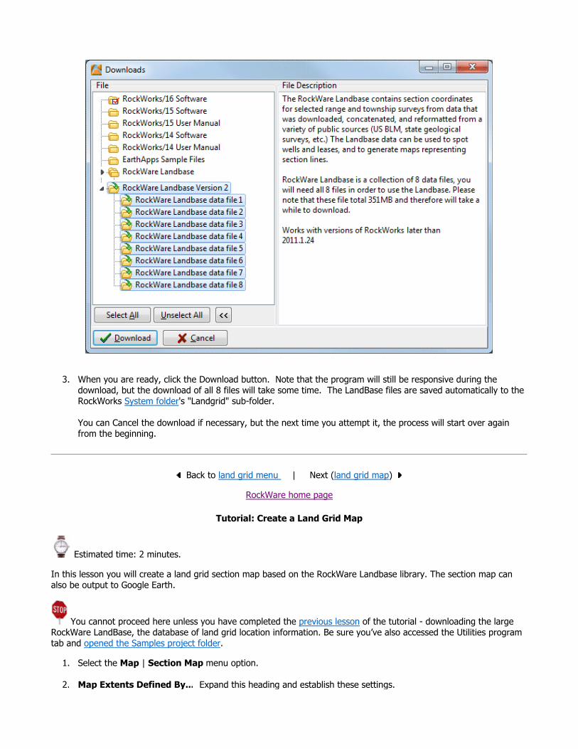
3. When you are ready, click the Download button. Note that the program will still be responsive during the download, but the download of all 8 files will take some time. The LandBase files are saved automatically to the RockWorks System folder's "Landgrid" sub-folder.
You can Cancel the download if necessary, but the next time you attempt it, the process will start over again from the beginning.
Back to land grid menu | Next (land grid map)
RockWare home page
Tutorial: Create a Land Grid Map
Estimated time: 2 minutes.
In this lesson you will create a land grid section map based on the RockWare Landbase library. The section map can also be output to Google Earth.
You cannot proceed here unless you have completed the previous lesson of the tutorial - downloading the large RockWare LandBase, the database of land grid location information. Be sure you’ve also accessed the Utilities program tab and opened the Samples project folder.
1. Select the Map | Section Map menu option.
2. Map Extents Defined By... Expand this heading and establish these settings.

a. Range & Township (Fast): Select this option. This tells RockWorks that we are going to limit the map extents by specific townships. Expand this heading.
Principal Meridian: This should be set to: 6If it is not, click on this prompt and click on the radio button in eastern Kansas. You will be returned to the menu with the Principal Meridian set to "6". Ranges:
Westernmost Range: Click on this item and type in: 70WEasternmost Range: Click on this item and type in: 70W
Townships: Southernmost Township: Click on this item and type in: 4SNorthernmost Township: Click on this item and type in: 3S
3. Map Options: Establish the appearance settings: a. Section Borders: Insert a check in this check-box so that the section lines will be plotted.
Expand this item and click to the right to set the line style to thin, and the color to red.
b. Fill Sections: Uncheck this. c. Section Labels: Check this box. Expand this heading.
Verbose: Remove this check-mark so that the labels will be short in length.
Include Acreages: Remove this check-mark also. Font Size: 2.0 (representing a percent of the size of the section). Font Color: red.
Opaque Background: uncheck this. d. Township Borders: Insert a check here.
Expand this to select thicker, blue lines for the Township boundaries.
e. Fill Townships: Uncheck this. f. Township Labels: Check this box, and expand this heading.
Decimal Fractions: Uncheck this
Verbose: Remove this check-mark so that the labels will be short in length. Font Size: 5.0Font Color: black
Opaque Background: uncheck this. g. Labeling Convention: Expand this
a. Township/Range: Click in this button. This just tells the program to plot the Township label first.
h. Border: Uncheck this option.
4. Click Process at the bottom of the Land Map window.
The program will read the location information from the LandBase and create a map illustrating the four selected Townships, each with 36 sections, and display it in a 2D plot window ("RockPlot2D"), where "flat" maps, logs, and other diagrams are displayed. The output map will use the project coordinate system and units.

11. Save the map: a. Choose the Save command from the RockPlot File menu. b. In the displayed prompt, enter the file name: reference-grid and click the Save button. The program
will stored the map under that file name, with an ".Rw2D" file name extension.
12. If you have Google Earth installed on your computer and would like to display this map in that program, click the
Google Earth button at the top of the map window.! Note that Google Earth is not installed with RockWorks; please visit www.earth.google.com for download and licensing information.In the displayed options window, choose the following options.
a. Drape: Click in the button - the map will lie along the ground surface in Google Earth. b. Transparent Background: Check this box so that the white map background is set to transparent. c. Click Process at the bottom of the window. d. If RockWorks displays a window confirming the output KMZ file name, click OK. e. Your map should be displayed as draped along the ground surface in the project area. f. If you would like to save this map in Google Earth, right-click on the Rw2D Map item under Temporary
Places, and select Save to My Places.
13. Back at RockWorks, you can close the map window using the close button ( ) in the upper-right corner.
Section Maps
Back to land grid menu | Next (spot RTS wells)
RockWare home page
Tutorial: Spot PLSS Well Locations and Map Them
Estimated time: 6 minutes.
In this lesson, you will learn how to spot wells that have their locations defined in terms of Public Land Survey descriptions (Range, Township, and Section); you will use the RockWare LandBase to convert this type of location information to actual X,Y coordinates in a UTM Easting and Northing format.

You cannot proceed here unless you have completed the "Download RockWare LandBase" section of the tutorial. Be sure you’ve also accessed the Utilities program tab and opened the Samples project folder.
1. Locate the Project Manager pane along the left edge of the program window. Here you'll see groupings of a variety of different RockWorks file types in the Samples folder.
3. Expand the Datasheet Files heading in the Project Manager. You'll see a long list of sample data files.
4. Locate the file "PLS_Points_to_XY.RwDat" - the list is alphabetical - and double-click on it. The program will load the contents of the data file into the Utilities datasheet.Note: you can also open .RwDat files into the Utilities datasheet using the File | Open command.
The program will display a listing of 13 wells that are described using land grid quarter/quarter or footage descriptions.
5. To spot the wells, select the Coords | Coordinate Converter (Multiple Points) command from the upper Utilities menu.
6. Input: On the left side of this window, you need to tell the program the format in which the source coordinates are recorded. Click the small down arrow and choose Public Land Survey.
7. Data Columns: Use these prompts along the left to select which columns contain what data. The name of the currently-selected datasheet column for each required input field is displayed below each prompt. To change a column name for any of the prompts simply click on the small down-arrow and select another column name. The prompts and column names you need to establish are listed here:
a. Meridian: Set to the column named Meridian. b. Range: Set to the column named Range. c. Township: Set to Township. d. Section: Set to Section. e. Description: Set to Legal.
8. Output: On the right side of the screen, you need to tell the program the format in which you want the output coordinates to be recorded. Click the down arrow and select UTM - Meters.

9. Data Columns: Use these prompts to select where the computed coordinates are to be listed. a. UTM Easting: Set to the column named 7 for recording of the computed X coordinates. b. UTM Northing: Set to the column named 8 for recording of the computed Y coordinates.
10. Universal Transverse Mercator Projection: Use these large buttons at the bottom of the window to choose: Datum = WGS-83 (NAD-83) Zone = 13
11. Click the OK button at the bottom of the Coordinate Converter window to proceed.
The program will compute the X and Y location coordinates for each well, in meters, based on the information stored in the reference land grid database. The computed coordinates will be listed in the Easting and Northing columns in the main datasheet, to the right of the Location column.
12. To create a simple point map of these wells, select the EZ Map command from the Utilities Map menu.
13. Use the Input Columns prompts along the left to establish data setup information. a. X (Easting): Set to UTM Easting. b. Y (Northing): Set to UTM Northing. c. Z (Elevation): This setting will be ignored since you won’t be plotting contours.
14. Symbols: Be sure this option is checked so that the map will include location symbols. Expand the Symbols heading and click on the Symbol Options button.
a. Column-Based: Be sure this option is selected. This tells the program to use symbols stored in a column in the datasheet to represent the map locations.
Symbol Column: Choose the datasheet column named Symbol which, as you might guess, tells the program where to read the symbols from. Dimensions: Choose Uniform Size, and enter a Size of 2. These dimensions represent a percent of the map width. In your own work, should you wish to increase the size of the symbols, just set the Size to a greater percentage.
b. Be sure the other Symbol options are not checked (Uniform, Circles, and Table-Based). c. Click OK to close this window.
15. Labels: Check this option to include labels with the symbols. Expand the Labels heading and click on the Labeling Options button.
a. Plot Label: Southeast: check this. Data Column: Choose the ID column - click on the small down-arrow to see a list of the data columns. You may need to scroll upward though the list to find the ID column.This tells the program to plot sample ID labels to the southeast of the symbols. Text Color: choose a color by clicking on the color box.
Opaque Background: Remove any check from this box.
b. Plot South Label, Plot Southwest Label, etc: The remaining Plot Label check-boxes should be cleared.
c. Font Size: Click here and set this to: 2d. The remaining default label options should work well.
e. Automatic Offset: Leave this option un-checked. (Note, though, that this is a very nifty tool to use in your own work. It prevents over-plotting in crowded maps.)
f. Click OK to close this window.
16. Back at the EZ Map window, make sure that the remaining map options are not checked:Contour Lines: off
Colored Intervals: offDecluster Points: off
Network: offBitmap: off

Borders: off
Interpolate Edge Points: off
17. Click the Process button at the bottom of the EZ Map window.
The program will display a very simple point map on the screen, in a RockPlot2D tab.
18. Save the map: a. Choose the File | Save command from the RockPlot menu. b. In the displayed prompt, enter the file name: Spot-points and click the Save button.
19. If you created a land grid map in part 2 of this section, you can combine this point map with the land grid map.Click on the File | Append command. The program will prompt you for the name of the map to append to this point map.
20. Locate and click on the file named reference-grid.Rw2D that you created earlier, and click the Open button.
RockWorks will read the contents of the land grid map and append it to the point map. The combined image will be displayed in a new window.
21. Expand the Layers pane by clicking on the small "+" button in the upper-right corner of the image pane.
22. Right-click on the Points layer and select Bring to Front from the pop-up menu. This will move the points and their labels to the foreground.
23. Save the new combined file using the File | Save command, and name this map grid and points
24. You may close this window ( ).
Converting Coordinates
See also: RockPlot2D Tutorial for lessons on editing maps
Back to land grid menu
RockWare home page
Tutorial: Analyze Component Data
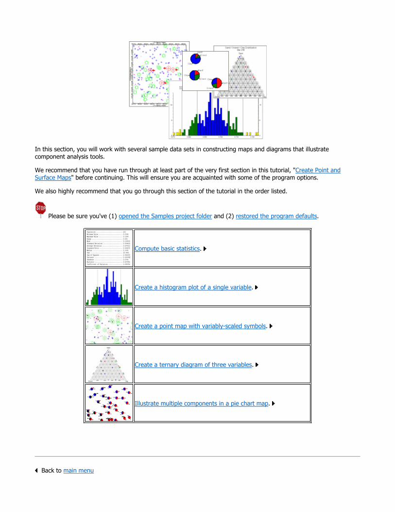
In this section, you will work with several sample data sets in constructing maps and diagrams that illustrate component analysis tools.
We recommend that you have run through at least part of the very first section in this tutorial, "Create Point and Surface Maps" before continuing. This will ensure you are acquainted with some of the program options.
We also highly recommend that you go through this section of the tutorial in the order listed.
Please be sure you've (1) opened the Samples project folder and (2) restored the program defaults.
Back to main menu
Compute basic statistics.
Create a histogram plot of a single variable.
Create a point map with variably-scaled symbols.
Create a ternary diagram of three variables.
Illustrate multiple components in a pie chart map.
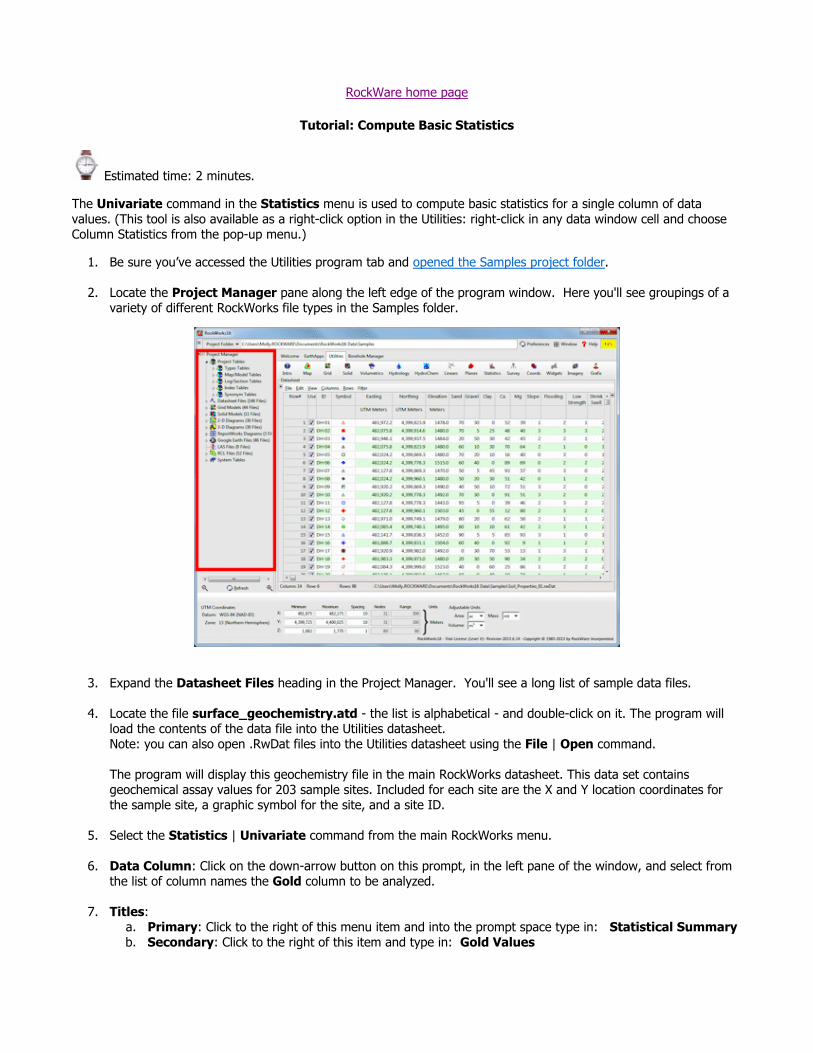
RockWare home page
Tutorial: Compute Basic Statistics
Estimated time: 2 minutes.
The Univariate command in the Statistics menu is used to compute basic statistics for a single column of data values. (This tool is also available as a right-click option in the Utilities: right-click in any data window cell and choose Column Statistics from the pop-up menu.)
1. Be sure you’ve accessed the Utilities program tab and opened the Samples project folder.
2. Locate the Project Manager pane along the left edge of the program window. Here you'll see groupings of a variety of different RockWorks file types in the Samples folder.
3. Expand the Datasheet Files heading in the Project Manager. You'll see a long list of sample data files.
4. Locate the file surface_geochemistry.atd - the list is alphabetical - and double-click on it. The program will load the contents of the data file into the Utilities datasheet.Note: you can also open .RwDat files into the Utilities datasheet using the File | Open command.
The program will display this geochemistry file in the main RockWorks datasheet. This data set contains geochemical assay values for 203 sample sites. Included for each site are the X and Y location coordinates for the sample site, a graphic symbol for the site, and a site ID.
5. Select the Statistics | Univariate command from the main RockWorks menu.
6. Data Column: Click on the down-arrow button on this prompt, in the left pane of the window, and select from the list of column names the Gold column to be analyzed.
7. Titles: a. Primary: Click to the right of this menu item and into the prompt space type in: Statistical Summaryb. Secondary: Click to the right of this item and type in: Gold Values

8. Minimum Filter: Remove any check-mark from this check-box.
9. Maximum Filter: Remove any check-mark from this check-box.
10. Click the Process button at the bottom of the window to perform the computations.
The program will scan the values in the Gold column in the datasheet and compute some basic statistics. The results are displayed in a text tab in the Options window.
Take note of the first 6 computations.
Population ........... 203Minimum Value ........ 0.0769Maximum Value ........ 0.1289Range ................ 0.052Mean ................. 0.100818Standard Deviation ... 0.009614
In the next step, we will display the gold values in a histogram plot, with mean and standard deviation displayed.
11. Close the text window, you don’t need to save the information.
Creating a Statistical Report
Back to component menu | Next (histogram)
RockWare home page
Tutorial: Create a Histogram Plot of a Single Variable
Estimated time: 2 minutes.
A frequency histogram is a graph that displays the distribution of real number values, read from a single datasheet column, by percent or actual occurrences.
! It is assumed that you have opened the "surface_geochemistry.RwDat" file as discussed in the previous lesson.
1. Click on the Statistics menu, and choose the Histograms | Single option.
2. Data Column: Click on the down-arrow button on this prompt, in the left pane of the window, and select from the list of column names the Gold column to be analyzed.
3. Titles: Expand this heading to establish the diagram titles: a. Primary: Click to the right of this menu item, and into the prompt space type: Goldb. Secondary: Click to the right of this item and type into the prompt space: Surface GeoChem Data
Set
4. Scaling + Bin Size: Expand this heading. a. Linear: Click in this radio button, and expand this heading.
Automatic: Choose this linear scaling option. This will set the bins to 1/10th the standard deviation. In your own work, if you prefer to declare the actual number of units for each bin, you can select the Manual option.
b. Confirm Range should be disabled.
5. Bin Colors: Expand this option to select how the diagram will be colored. a. Discrete: Choose this option. This will apply different colors to the bars in the graph based on their

relationship to the mean and standard deviation. You can expand this heading to view the default colors.
6. Minimum Filter: off
Maximum Filter: off
7. Plot Statistics: Check this box, and expand it a. Font: Click here to set the Size to 2.0 and the text color to your choice. b. Verbose: Check this option.
8. Plot X-Axis Labels: Check this setting.
9. Plot Y-Axis Labels: Check this option, and expand it.
a. Plot as Percentages: Un-check this box. This tells the program to plot actual occurrences rather than percent.
10. Statistical Legend: off
11. Fixed Diagram Size: off
12. Click the Process button at the bottom of the Histogram window.
The program will build the frequency histogram and display it in a new RockPlot2D window on the screen. RockPlot2D is the plotting program for "flat" maps, logs, and other diagrams.
For this type of geochemistry data, the values of interest lie in the Slightly Anomalous and Anomalous groupings, particularly the latter, beyond the mean plus 2 standard deviations.
13. Look closely at this group. This plot shows four samples with anomalous (high) gold values.
Let's take a look at where these samples lie; the next tutorial lesson teaches you how to build a proportional symbol map, in which those sites with larger gold values are plotted with larger symbols.
14. If you wish to save this plot, choose the File | Save command from the RockPlot menu, enter a name such as: gold histogram and click the Save button.
15. Close this window ( ).
Frequency Histograms

Back to component menu | Next (variable symbol map)
RockWare home page
Tutorial: Create a Point Map with Variably-Scaled Symbols
Estimated time: 5 minutes.
Variably-scaled symbol maps are point (symbol) maps in which the size of the symbols vary according to a measured value at each site, read from the main datasheet. This can be an effective tool to visualize quickly sites with low versus high values.
! It is assumed that you have opened the "Surface Geochemistry" data file as discussed in the first lesson of this section.
1. Choose the EZ-Map command from the Utilities Map menu.
2. Input Columns: In the prompts along the left side of the window, be sure the following columns are selected. (If the wrong column title is displayed, just click on the down-arrow and scroll up or down to the correct column title.)
a. X (Easting): Easting b. Y (Northing): Northing c. Z (Elevation): Gold (Though, since you are not generating contours, this setting will be ignored.)
3. Symbols: Be sure this option is checked so that the map will include location symbols. Expand the Symbols heading and click on the Symbol Options button.
a. Uniform: Uncheck this b. Column-Based: Be sure this option is selected. This tells the program to use symbols stored in a
column in the datasheet to represent the map locations. Symbol Column: Choose the datasheet column named Symbol which tells the program where to read the symbols from. Dimensions:
Variable: Choose this option to request that the symbols be sized differently, based on a measured value. Scaling: Data Column: Click here and choose Gold. This tells the program to look at the values in the Gold column to know how to scale the symbols.
Range: Click in this radio button. Minimum: Type in: 0.25Maximum: Type in: 5.0These settings indicate that the sample site(s) with the smallest measured Gold value is to be displayed in the map with its symbol sized at 0.25 percent of the map width. The sample site(s) with the largest Gold value is to be plotted with its symbol sized at 5 percent of the map width. All sites with Gold values in between the minimum and maximum are to be plotted with their symbols scaled in a linear fashion between these extremes.
c. Circles: Unchecked. d. Table-Based: Unchecked.
e. Images: Unchecked. f. Click OK to close this window.
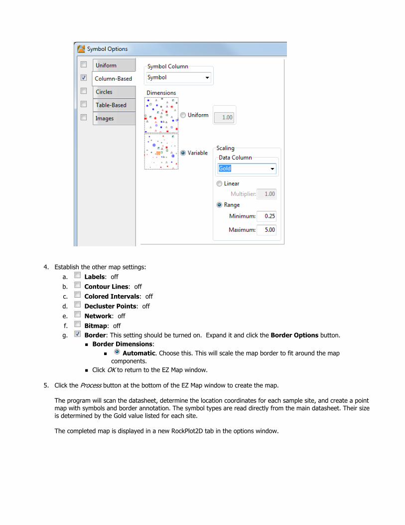
4. Establish the other map settings: a. Labels: off
b. Contour Lines: off c. Colored Intervals: off d. Decluster Points: off
e. Network: off f. Bitmap: off g. Border: This setting should be turned on. Expand it and click the Border Options button.
Border Dimensions: Automatic. Choose this. This will scale the map border to fit around the map
components. Click OK to return to the EZ Map window.
5. Click the Process button at the bottom of the EZ Map window to create the map.
The program will scan the datasheet, determine the location coordinates for each sample site, and create a point map with symbols and border annotation. The symbol types are read directly from the main datasheet. Their size is determined by the Gold value listed for each site.
The completed map is displayed in a new RockPlot2D tab in the options window.
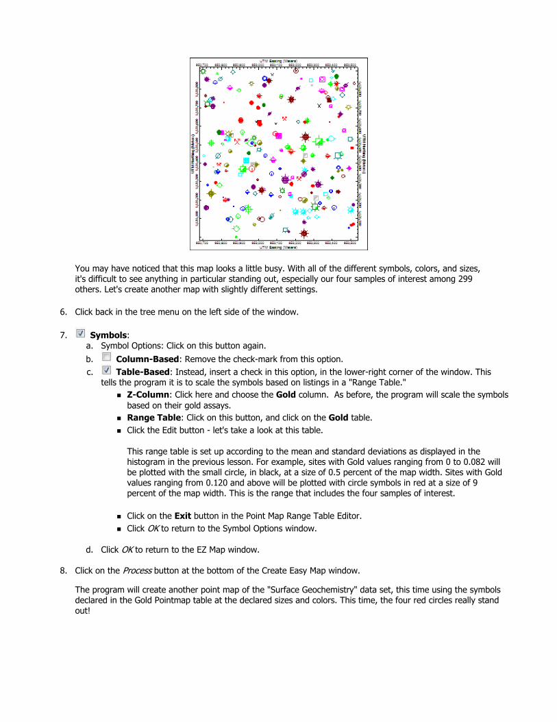
You may have noticed that this map looks a little busy. With all of the different symbols, colors, and sizes, it's difficult to see anything in particular standing out, especially our four samples of interest among 299 others. Let's create another map with slightly different settings.
6. Click back in the tree menu on the left side of the window.
7. Symbols: a. Symbol Options: Click on this button again.
b. Column-Based: Remove the check-mark from this option. c. Table-Based: Instead, insert a check in this option, in the lower-right corner of the window. This
tells the program it is to scale the symbols based on listings in a "Range Table." Z-Column: Click here and choose the Gold column. As before, the program will scale the symbols based on their gold assays. Range Table: Click on this button, and click on the Gold table. Click the Edit button - let's take a look at this table.
This range table is set up according to the mean and standard deviations as displayed in the histogram in the previous lesson. For example, sites with Gold values ranging from 0 to 0.082 will be plotted with the small circle, in black, at a size of 0.5 percent of the map width. Sites with Gold values ranging from 0.120 and above will be plotted with circle symbols in red at a size of 9 percent of the map width. This is the range that includes the four samples of interest.
Click on the Exit button in the Point Map Range Table Editor. Click OK to return to the Symbol Options window.
d. Click OK to return to the EZ Map window.
8. Click on the Process button at the bottom of the Create Easy Map window.
The program will create another point map of the "Surface Geochemistry" data set, this time using the symbols declared in the Gold Pointmap table at the declared sizes and colors. This time, the four red circles really stand out!

9. Save this plot if you wish by choosing the RockPlot File | Save command, entering a name such as: gold-map and clicking the Save button.
10. Close this window using the Close button ( ).
EZ Maps
Back to component menu | Next (ternary diagram)
RockWare home page
Tutorial: Create a Ternary Diagram of Three Variables
Estimated time: 2 minutes.
The Ternary command in the Stats menu is used to create a ternary plot for three variables read from the main datasheet. We will use a different sample file than the "GeoChem" data set used in the earlier lessons of this section.
1. Be sure you’ve accessed the RockWorks Utilities datasheet and opened the Samples project folder.
2. Open a new sample file: a. In the Project Manager pane along the left edge of the program window, expand the Datasheet File
heading if necessary. b. Look for the file named Soil_Properties_01.RwDat. c. Double-click on that file name to open it. d. If you are prompted to save changes to the existing datasheet, click No.
The program will display this file in the main Utilities datasheet. This data set contains an ID, symbol, X and Y location coordinates, and elevation for each sample site. It then lists sand, gravel, and clay percentages, Ca and Mg measurements, several geotechnical measurements, and soil colors. For this exercise, we will display the sand/gravel/clay components in the ternary plot.
3. Select the Ternary | Single command from the Statistics menu.
4. Input Columns: Use these prompts along the left to establish data setup. The name of the currently-selected datasheet column for each required input field is displayed below each prompt. To change a column name for any of the prompts simply click on the small down-arrow and select another column name. The prompts and column names you need to establish are listed here:
a. Upper Vertex: Set to the column named Sand for the data to be represented in the upper vertex in the diagram.
b. Left Vertex: Set to the column Gravel for the data to be represented in the lower-left vertex in the diagram.
c. Right Vertex: Set to the column Clay for the data to be represented in the lower-right vertex in the diagram.
5. Titles: Expand this heading to establish the diagram and axis titles. (These may already be displayed as defaults.)
a. Primary: Click here and type in: Sand/Gravel/Clay Distribution and click OK. b. Secondary: Click here and type in: Site 27B and click OK. c. Vertex Labeling: Expand this option and set the vertex titles as shown:
Upper Vertex: SandLeft Vertex: GravelRight Vertex: Clay
6. Symbols: Check this option and expand it. a. Symbol Options: Click this button. b. Column-Based: Check this option.
Symbol Column: Click here and choose the "Symbol" column. Dimensions: Choose Uniform, at a size of 3.0.
c. Be sure Uniform, Circles, Table-Based, and Images are not checked. d. Click OK to close the Symbol Options window.
7. Other options: a. Labels: unchecked
b. Contour Lines: unchecked c. Colored Intervals: unchecked
In your own work you may want to include point labels, if your data set is not this large. You may also want to request line and/or color-filled contours to illustrate point density.
8. Gridding Options can be ignored since you have not selected any contouring.
9. Annotations & Embellishments: Click on the Options button to the right. Subdivisions: Click on this item.
Major Subdivisions: Check this option. Click on the Line Styles sample to select thin, black lines.
Minor Subdivisions: Be sure this is checked. Click on the Line Styles sample to select thin lines, and set the color to light gray. Intervals: Choose Major = 10% / Minor = 2%
Perimeter: Check this option. Axis Labeling: Check this option, and click on the tab to choose 20% for the interval. Tick Marks: Check this option, and choose 20% for Increments and Internal for the locations.
10. Classification Overlays: Un-check this. These new options will plot a pre-defined diagram in the background with your data points and/or contours in the foreground. The currently available templates include Folk's (1954) siliclastic classification system, Schlee's (1973 - after Shepard) siliclastic classification system, Shepard's 1954 siliclastic classification system, and the USDA soil classification system.
11. Click OK to close the Annotation & Embellishment Options window.

12. Click the Process button at the bottom of the Ternary Diagram window to proceed.
The program will read the values from the Sand, Gravel, and Clay data columns. Each sample will be normalized such that the three components add up to 100%. The symbol for that sample will be plotted at that point in the diagram, with 100% sand represented at the top, 100% gravel represented at the left vertex, and 100% clay at the right vertex.
In the example below, the single sample contains 60% sand, 30% shale, and 10% clay.
11. Close this window by clicking the Close button ( ). Answer No to the save-file prompt.
Ternary Diagrams
Back to component menu | Next (pie chart map)
RockWare home page
Tutorial: Illustrate Multiple Components in a Pie Chart Map
Estimated time: 2 minutes.
A Pie Chart Map is a type of symbol map in which each map location is marked with a small pie chart representing a user-selected number of components for that location. We will display the sand-gravel-clay components by site.
! You need to have completed the previous lesson before continuing.
1. With the "Soil_Properties_01.RwDat" data set displayed in the main Utilities datasheet, select the Map | Pie Chart Map option.
2. Input Columns: Use these prompts along the left to tell RockWorks which column contains which data. To change a column name for any of the prompts simply click on the small down-arrow and select another column name. The prompts and column names you need to establish are listed here:
a. Easting (X): Set to the column Easting. b. Northing (Y): Set to the column Northing.
3. Set up these components in the large pane of the window.

a. Plot Component #1: Checked. This tells the program to include the data for "component 1" in the pie symbols. Expand this heading to access the settings.
Column: Click to the right to set this to the Sand column. Color: Choose a color for this data.
Explode: unchecked. b. Plot Component #2: Checked. This tells the program to include the data for "component 2" in the
pie symbols. Column: Click to the right to set this to the Gravel column. Color: Choose a color for this data.
Explode: unchecked. c. Plot Component #3: Check this, so that the program will include another component in the
symbols. Column: Click to the right to set this to the Clay column. Color: Choose a color for this data.
Explode: unchecked.
d. Plot Component 4 – Plot Component 9: Be sure these are all un-checked.
4. Radius: Expand this heading to set the Inner Radius to 0.0 and the Outer Radius to 2.0.
5. Plot Labels : Insert a check here to include labels with the pie symbols.
6. Border : Uncheck this.
7. Click the Process button at the bottom of the window to create the map.
The program will read the records in the data set and create for each record a small pie chart illustrating the relative Sand-Gravel-Clay components. The mini-pie-charts will be placed at their sample's X,Y coordinates in the map.
Note how the sandy soils in the southeast grade into clayey soils in the north and west.
If you are interested in adding border annotation to this map, save the map as instructed below, and then jump to the RockPlot2D tutorial.
7. Save this map by choosing the File | Save command from the RockPlot menu, entering the file name: pie-map and clicking the Save button.

8. Close this window ( ).
Pie Chart Maps
Back to component menu
RockWare home page
Tutorial: RockWorks EarthApps
Choose a lesson by clicking on the link or " ".
Back to main tutorial menu
RockWare home page
Tutorial: RockWorks EarthApps Introduction
The RockWorks EarthApps contains a row-and-column datasheet window designed for entering miscellaneous spatial data. These data can include simple XY data for generating point maps, bearing and dip data for strike and dip maps, image names, line endpoints, and many more.
The EarthApps program is accessed by clicking on the "EarthApps" tab along the top edge of the program window.
Introduction to the RockWorks EarthApps
Open a project folder
Restore the Program Defaults
Create point maps in Google Earth
Create flyovers in Google Earth

This data window has its own suite of menu options. The data you enter into the EarthApps datasheet can be used to create many different types of maps and diagrams.
"Borehole" data, consisting of downhole lithology, stratigraphy, geochemistry, geophysical and other measurements are entered into the separate "Borehole Manager", discussed in a separate section of this tutorial (click here to jump to that lesson set). The Borehole Manager tools are not available if you did not purchase a RockWorks license (Level 3+).
Back to main menu | Next (Open project)
RockWare home page
Tutorial: Open an EarthApps Project Folder
Estimated time: 1 minute.
1. First, access the RockWorks EarthApps program and datasheet by clicking on its button that lies near the top of the RockWorks window.
2. Look at the Project Folder listing right below the upper menu items.
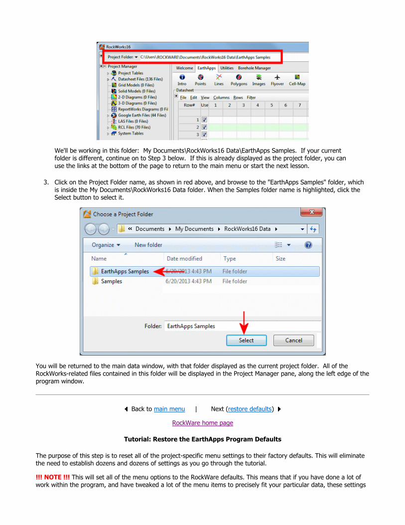
We'll be working in this folder: My Documents\RockWorks16 Data\EarthApps Samples. If your current folder is different, continue on to Step 3 below. If this is already displayed as the project folder, you can use the links at the bottom of the page to return to the main menu or start the next lesson.
3. Click on the Project Folder name, as shown in red above, and browse to the "EarthApps Samples" folder, which is inside the My Documents\RockWorks16 Data folder. When the Samples folder name is highlighted, click the Select button to select it.
You will be returned to the main data window, with that folder displayed as the current project folder. All of the RockWorks-related files contained in this folder will be displayed in the Project Manager pane, along the left edge of the program window.
Back to main menu | Next (restore defaults)
RockWare home page
Tutorial: Restore the EarthApps Program Defaults
The purpose of this step is to reset all of the project-specific menu settings to their factory defaults. This will eliminate the need to establish dozens and dozens of settings as you go through the tutorial.
!!! NOTE !!! This will set all of the menu options to the RockWare defaults. This means that if you have done a lot of work within the program, and have tweaked a lot of the menu items to precisely fit your particular data, these settings

will be lost. If this is a worry for you, you might consider the following: Before restoring the factory defaults, you can use the Preferences | Export Menu Settings option to store all of your current settings in a file that can later be imported back into the program using the Preferences | Import Menu Settings option.
Step-by-Step Summary
1. If you have just installed RockWorks you can skip this step because program defaults have already been established. (Click the Next button below.)
2. If you’ve been running RockWorks for a while (or if you aren’t sure), you should click on the Preferences menu and choose Reset Menu Settings.
3. Establish these menu options:
Reset Global Settings: Uncheck this item. Reset Project Settings: Check this item. It will reset the project-specific settings to factory
defaults. 4. Click on the Process button at the bottom of the window. 5. Click the Yes button in the confirmation window. 6. You'll be returned to the EarthApps window.
Back to main menu | Next (point maps)
RockWare home page
Tutorial: Create Point Maps for Google Earth
These lessons will focus on the tools in the EarthApps Points menu: icon maps, scaled cone maps, and 3D strike and dip maps.
Pick a lesson by clicking on its its link or arrow ( ). We recommend going through these lessons in the order listed.
If this is the first lesson you’ve done, please be sure you’ve (1) opened a project folder and (2) restored the program defaults.
Open a data file
Create a simple icon map
Create a scaled cone map
Create a 3D strike and map

Back to main menu
RockWare home page
Tutorial: Open an XY Point Data File
Estimated time: 1 minute.
1. Access the RockWorks EarthApps datasheet and open the Samples project folder, as described earlier. (Remind me… )
2. Locate the Project Manager pane along the left edge of the program window. Here you'll see groupings of a variety of different RockWorks file types in the Samples folder.
3. Expand the Datasheet Files heading in the Project Manager. You'll see a long list of sample data files.
4. Locate the file "Icons_Simple_01.RwDat" in the alphabetical list, and double-click on it. The program will load the contents of the data file into the datasheet.
This particular file contains sample IDs, and X and Y location coordinates in longitude and latitude.
! RockWorks permits you to organize your data almost any way you like. Any time you want to create a map or diagram, you can specify which columns in the datasheet contain what type of data.
5. View the Column Parameters: Right-click in the gray column heading for the Sample ID column (or select Columns | Column Properties). The program will display the column parameters window.

This is where you can assign the column title and column type. The Sample ID column is a "Generic" text column.
6. Click the green arrow at the top of the window again to advance to the Easting column.
This column contains geographic coordinates. Here you can specify the coordinate type and the units.
! X and Y coordinate columns must have type and units selected for map creation. In this example, the coordinates are recorded in alongitude and latitude system, in decimal degrees.
7. Click the green arrow to advance to the Northing column - it's also set as a Geographic/Spatial column, with coordinate system and units selected as decimal degrees.
8. Click OK to close the Column Settings window.
Opening an Existing Datasheet, Changing Column Titles and Styles, Using the Project Manager
Back to point map menu | Next (icon map)
RockWare home page
Tutorial: Create a Simple Icon Map in Google Earth
Estimated time: 3 minutes.
If this is the first lesson you’ve done, please be sure you've opened the Icons_Simple_01.RwDat data file.
! These lessons require that you have Google Earth installed on your computer. Google Earth is not installed along with RockWorks. Please visit www.earth.google.com for download and licensing information.
1. Click on the Points menu at the top of the EarthApps window, and choose the Icons | Simple menu option.
2. Input Columns: In the prompts along the left side of the window, be sure the following columns are selected. This tells RockWorks which columns contain which data. (If the wrong column title is displayed, just click on the down-arrow and scroll up or down to the correct column title.)
X: Longitude Y: Latitude
Next, set up the map layers in the next pane to the right, where there's a "tree menu" with a variety of map options. Expand and collapse headings by clicking on the small "+" or "-" buttons.
3. Icon: This setting establishes the icon design to be used to represent the sample locations in the Google Earth. Click on the existing picture to the right to choose an icon design for the sites.
4. Include Labels: Check this option to include labels with the icons. Expand the heading to access the label options.
Label Column: Click to the right to select the name of the column in the data file that contains the text to be used as the labels. Choose the Sample ID column. Label Color: Click to the right, on the color sample box, to choose a color for the labels. When displayed in Google Earth, light colors are usually preferable. (Defaut = white) Label Size: Set this to 1.0 (Rule of thumb: 0.5 will create small labels, 2.0 large labels.)
5. Click the Process button at the bottom of the Icon Map window.
The program will create a KML file listing the icons at the point locations. It will create a KMZ (zip) file containing the KML file. The Google Earth KML and KMZ file names will be assigned automatically.
6. If RockWorks displays the KMZ name in a popup window for your reference, you can confirm: Automatically load file into Google Earth: Be sure this is checked if you want to display the output at this time. Show this message every time a KMZ File is Created: If checked, this window will be displayed each time a Google Earth output is created. Uncheck this if you prefer not to see this window in the future.(Both of these settings are also available via the Preferences menu.)Click OK to continue or Cancel to cancel the operation.
The resulting map will be displayed in Google Earth, if requested. The "Icons" will be listed under Temporary Places on the left side of the Google Earth display. You can expand the heading to see the individual sites, and the checkboxes can be used to turn individual sites as well as the entire group on/off.
Feel free to take a moment to explore this display.

Click on the Icon Maps link below for information about other types of icon maps you can create.
7. If you would like to save this group of icons, right-click on it and choose Save to My Places.
8. You can leave the Google Earth window open if you'll be doing the next lesson.
Icon Maps
Back to point map menu | Next (Cone map)
RockWare home page
Tutorial: Create a Scaled Cone Map in Google Earth
Estimated time: 3 minutes.
In this lesson, you will load a dataset that has X and Y location coordinates and a variety of measured values. You will create a map in which cone symbols are placed at the map locations, scaled in size and color based on the magnitude of one of the components in the listing. This is a quick way to quickly visualize the spatial and measured values in your data.
1. Return to the RockWorks EarthApps program window (you can leave Google Earth open if you just completed the Icon Map lesson).
2. Return to the Project Manager pane along the left side of the program window, and, under the Datasheet Files heading, look for the "Cones_Proportional_01.RwDat" sample file. Double-click on this file name to open it into the datasheet.
This file contains stream sediment data. We'll use this to display samples as scaled cones within Google Earth.
3. Click on the Points menu at the top of the EarthApps window, and choose the Cones | Porportional menu option.
4. Input Columns: In the prompts along the left side of the window, be sure the following columns are selected. This tells RockWorks which columns contain which data. (If the wrong column title is displayed, just click on the down-arrow and scroll up or down to the correct column title.)
X: LongitudeY: LatitudeZ: AU_PPM: For this map we'll represent the gold concentrations.
Next, in the settings pane to the right, establish these options.
5. Style: Choose Downward Pointing Cones.
6. Radii (Meters): This settings establishes the radius of the cones in meters. Proportional (Based on Z Column): Click in this radio button.
Minimum Radius: Click to the right and type in: 10Maximum Radius: Click to the right and type in: 1000This tells RockWorks to plot the cones where the smallest values were measured with a radius of 10 meters and those where the highest values were measured a radius of 1000 meters. The cones will be scaled automatically between these radii for intermediate values.
7. Height (Meters): This settings establishes the height of the cones in meters. Proportional (Based on Z Column): Click in this radio button.

Minimum Height: Click to the right and type in: 10Maximum Height: Click to the right and type in: 2000This tells RockWorks to plot the cones where the smallest values were measured with a height of 10 meters and those where the highest values were measured a radius of 2000 meters. As above, the height of the cones where intermediate values are listed will be scaled automatically.
8. Color: Proportional (Based on Z Column): Click in this radio button. This tells Rockworks to plot low-value cones in cool colors, high-value cones in hot colors, and intermediate cones colored gradationally in between.
9. Include Labels: Check this option to include labels with the icons. Expand the heading to access the label options.
Label Column: Click to the right to select the name of the column in the data file that contains the text to be used as the labels. Choose the AU_PPM column. Label Color: Click to the right, on the color sample box, to choose a color for the labels. When displayed in Google Earth, light colors are usually preferable. (Defaut = white) Label Size: Set this to 1.0 (Rule of thumb: 0.5 will create small labels, 2.0 large labels.)
10. Click the Process button at the bottom of the Cone Map window.
The program will create a KML file listing the cones at the point locations. It will create a KMZ (zip) file containing the KML file. The Google Earth KML and KMZ file names will be assigned automatically. Be patient - it will take a moment to generate the map for the 3626 samples in this datasheet.
11. If RockWorks displays the KMZ name in a popup window for your reference, you can confirm: Automatically load file into Google Earth: Be sure this is checked if you want to display the output at this time. Show this message every time a KMZ File is Created: If checked, this window will be displayed each time a Google Earth output is created. Uncheck this if you prefer not to see this window in the future.(Both of these settings are also available via the Preferences menu.)Click OK to continue or Cancel to cancel the operation.
The resulting map will be displayed in Google Earth, if requested. The "Cones" layer will be listed under Temporary Places on the left side of the Google Earth display.
12. Use your navigation tools in Google Earth to zoom in to the map area; you can also just double-click in the center of the display to zoom in. You can use your mouse to rotate the image to the left, right, up, and downward. Notice how the sites with the small values are shown with small cones, and those with high gold values are shown with large cones.
13. If you would like to save this map, right-click on it and choose Save to My Places.
14. You can leave the Google Earth window open if you'll be doing the next lesson.
Click on the Cone Maps link below for information about other types of cone maps you can create.
Cone Maps
Back to point map menu | Next (strike and dip map)
RockWare home page

Tutorial: Create a 3D Stike and Dip Map in Google Earth
Estimated time: 3 minutes.
In this lesson, you will load a dataset that has X and Y location coordinates, altitude above ground, strike and dip measurements at those sites, and radius, thickness and color values. You will create a map in which disk symbols are placed at the map locations, scaled in size and color.
1. Return to the RockWorks EarthApps program window (you can leave Google Earth open if you just completed the Cone Map lesson).
2. Return to the Project Manager pane along the left side of the program window, and, under the Datasheet Files heading, look for the "StrikeDip_3D_Advanced_01.RwDat" sample file. Double-click on this file name to open it into the datasheet.
3. Click on the Points menu at the top of the EarthApps window, and choose the Strike & Dip | 3D Disks (Advanced) menu option.
4. Input Columns: In the prompts along the left side of the window, be sure the following columns are selected. Easting: XNorthing: YAltitude: AltitudeDirection: Strike (Azimuth)Dip: DipRadius: RadiusThickness: ThicknessColor: Color
Next, in the settings pane to the right, establish these options.
5. Direction Represents: Choose Strike. This setting tells RockWorks that the directions listed in the datasheet represent the strike of the planar data, and that that the dip direction is 90 degrees clockwise of the listed azimuth.
6. Declination Correction: This should be set to 0.
7. Click the Process button at the bottom of the Strike & Dip Disks window.
The program will create a KML file listing the disks at the point locations, at the indicated orientation and dip angle, using the color and size you've specified in the datasheet. It will create a KMZ (zip) file containing the KML file. The Google Earth KML and KMZ file names will be assigned automatically.
8. If RockWorks displays the KMZ name in a popup window for your reference, you can confirm: Automatically load file into Google Earth: Be sure this is checked if you want to display the output at this time. Show this message every time a KMZ File is Created: If checked, this window will be displayed each time a Google Earth output is created. Uncheck this if you prefer not to see this window in the future.(Both of these settings are also available via the Preferences menu.)Click OK to continue or Cancel to cancel the operation.
The resulting map will be displayed in Google Earth, if requested. The "Disks" group will be listed under Temporary Places on the left side of the Google Earth display.
9. Unlike the previous two maps which covered a large area, this map covers a relatively small space - use your navigation tools in Google Earth to zoom out of the map area.

10. If you would like to save this map, right-click on the "Disks" heading under Temporary Places and choose Save to My Places.
11. Click on the Strike and Dip Maps link below for information about other types of strike and dip maps you can create.
! Tip: In the EarthApps Samples project folder, there are sample datasheet files for all of the EarthApps programs - just look for the file with the same (or similar) name as the program. For example, for the Points | Strike & Dip | 2D Symbols program, you would open the "StrikeDip_2D_01.RwDat" file.
! Tip: Also in the EarthApps Samples project folder, there are menu settings files for all of the sample datasheets. When you select one of the program options, click on the Menu button at the top of the screen, click on Load from RCL, and browse for the ".rcl" file with the same name as the datasheet.
RockWorks will load the menu settings listed there - just review them and click the Process button!
12. Feel free to take a break from the tutorial if you'd like to experiment with some of the other Point map sample files.
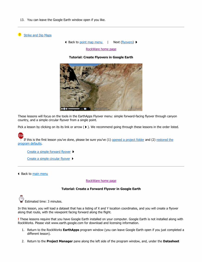
13. You can leave the Google Earth window open if you like.
Strike and Dip Maps
Back to point map menu | Next (flyovers)
RockWare home page
Tutorial: Create Flyovers in Google Earth
These lessons will focus on the tools in the EarthApps Flyover menu: simple forward-facing flyover through canyon country, and a simple circular flyover from a single point.
Pick a lesson by clicking on its its link or arrow ( ). We recommend going through these lessons in the order listed.
If this is the first lesson you’ve done, please be sure you’ve (1) opened a project folder and (2) restored the program defaults.
Create a simple forward flyover
Create a simple circular flyover
Back to main menu
RockWare home page
Tutorial: Create a Forward Flyover in Google Earth
Estimated time: 3 minutes.
In this lesson, you will load a dataset that has a listing of X and Y location coordinates, and you will create a flyover along that route, with the viewpoint facing forward along the flight.
! These lessons require that you have Google Earth installed on your computer. Google Earth is not installed along with RockWorks. Please visit www.earth.google.com for download and licensing information.
1. Return to the RockWorks EarthApps program window (you can leave Google Earth open if you just completed a different lesson).
2. Return to the Project Manager pane along the left side of the program window, and, under the Datasheet

Files heading, look for the "Flyover_Simple_Forward_01.RwDat" sample file. Double-click on this file name to open it into the datasheet.
This file contains a simple listing of map coordinates in longitude and latitude coordinates.
3. Click on the Flyover menu at the top of the EarthApps window, and choose the Simple: Camera Looking Forward menu option.
4. Input Columns: In the prompts along the left side of the window, be sure the following columns are selected. X (Easting): X(Easting) Y (Northing): Y (Northing)
In the settings pane to the right, establish these options.
5. In the settings pane to the right, establish these options. Tour Title: Click to the right and type in: Colorado River.Time (Seconds) Between Points: This establishes the pace of the flyover. Click to the right and type in: 1.0Altitude (Meters - Relative to Ground): This defines how high above the ground surface, in meters, that you want to "fly". Click to the right and enter: 100.0Tilt: This defines the "camera" angle. Enter: -15 for 15 degrees below horizontal (looking downward). Pan Smoothing Factor: Click to the right and enter: 1Note that a flyover with smoothing of "2" will create much less camera-bounce around sharp corners than a flyover with smoothing of "0". Beware that high smoothing can cut tight corners.
6. Click the Process button at the bottom of the flyover window.
The program will create a KML file listing the flyover path along the datasheet route. It will create a KMZ (zip) file containing the KML file. The Google Earth KML and KMZ file names will be assigned automatically.
7. If RockWorks displays the KMZ name in a popup window for your reference, you can confirm: Automatically load file into Google Earth: Be sure this is checked if you want to display the output at this time. Show this message every time a KMZ File is Created: If checked, this window will be displayed each time a Google Earth output is created. Uncheck this if you prefer not to see this window in the future.(Both of these settings are also available via the Preferences menu.)Click OK to continue or Cancel to cancel the operation.
The resulting flyover will be displayed in Google Earth, if requested. The "Flyover" group will be listed under Temporary Places on the left side of the Google Earth display. You'll see the flyover controls in the lower-left corner of the screen.
8. Click the Play button to start the flyover sequence. Click the Pause button to pause the flight.
9. If you would like to save this flyover, right-click on it and choose Save to My Places.
10. Leave the Google Earth window open for the next lesson.
Flyover Summary
Back to flyover menu | Next (circular flyover)
RockWare home page
Tutorial: Create a Circular Flyover from a Single Point
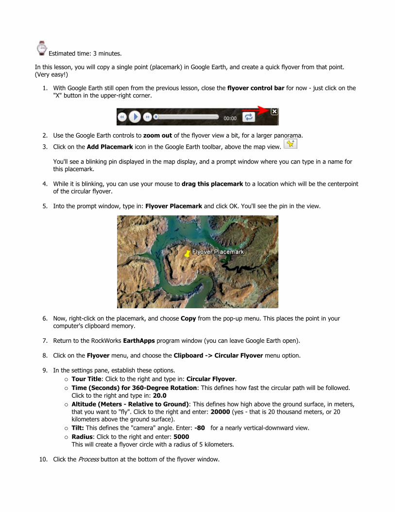
Estimated time: 3 minutes.
In this lesson, you will copy a single point (placemark) in Google Earth, and create a quick flyover from that point. (Very easy!)
1. With Google Earth still open from the previous lesson, close the flyover control bar for now - just click on the "X" button in the upper-right corner.
2. Use the Google Earth controls to zoom out of the flyover view a bit, for a larger panorama.
3. Click on the Add Placemark icon in the Google Earth toolbar, above the map view.
You'll see a blinking pin displayed in the map display, and a prompt window where you can type in a name for this placemark.
4. While it is blinking, you can use your mouse to drag this placemark to a location which will be the centerpoint of the circular flyover.
5. Into the prompt window, type in: Flyover Placemark and click OK. You'll see the pin in the view.
6. Now, right-click on the placemark, and choose Copy from the pop-up menu. This places the point in your computer's clipboard memory.
7. Return to the RockWorks EarthApps program window (you can leave Google Earth open).
8. Click on the Flyover menu, and choose the Clipboard -> Circular Flyover menu option.
9. In the settings pane, establish these options. Tour Title: Click to the right and type in: Circular Flyover.Time (Seconds) for 360-Degree Rotation: This defines how fast the circular path will be followed. Click to the right and type in: 20.0Altitude (Meters - Relative to Ground): This defines how high above the ground surface, in meters, that you want to "fly". Click to the right and enter: 20000 (yes - that is 20 thousand meters, or 20 kilometers above the ground surface).Tilt: This defines the "camera" angle. Enter: -80 for a nearly vertical-downward view. Radius: Click to the right and enter: 5000This will create a flyover circle with a radius of 5 kilometers.
10. Click the Process button at the bottom of the flyover window.

The program will create a KML file with the flyover around the point that you had copied to the clipboard. It will create a KMZ (zip) file containing the KML file. The Google Earth KML and KMZ file names will be assigned automatically.
11. If RockWorks displays the KMZ name in a popup window for your reference, you can confirm: Automatically load file into Google Earth: Be sure this is checked if you want to display the output at this time. Show this message every time a KMZ File is Created: If checked, this window will be displayed each time a Google Earth output is created. Uncheck this if you prefer not to see this window in the future.(Both of these settings are also available via the Preferences menu.)Click OK to continue or Cancel to cancel the operation.
The resulting flyover will be displayed in Google Earth, if requested. The "Flyover" group will be listed under Temporary Places on the left side of the Google Earth display. You'll see the flyover controls in the lower-left corner of the screen.
12. Click the Play button to start the flyover route. Click the Pause button to pause the flight.
13. If you would like to save this flyover, right-click on it and choose Save to My Places.
Flyover Summary
Back to flyover menu
RockWare home page
Tutorial: Plot and Manipulate 2D Maps and Diagrams - RockPlot2D
RockPlot2D is the plotting program for "flat" RockWorks diagrams, such as plan-view maps, 2D cross sections, and miscellaneous diagrams (ternary plots, etc.). Whenever a diagram like this is created, it will be plotted automatically in a RockPlot2D tab in the Options window. RockPlot2D can also be displayed as a stand alone window (not embedded in the Options window).
RockPlot contains many display, printing, and manipulation features. Choose a lesson by clicking on the link or icon " ".
If this is the first lesson set you’ve done, please be sure you’ve (1) opened a project folder, and (2) restored the program defaults.
Open, "zoom" into, and combine maps.

Annotate the map.
Measure distances on the map.
Edit the map.
Export the map and insert it into a document.
Export the map to Google Earth.
Print the map.
See also
The RockPlot3D Tutorial for lessons on the 3D plotting program in RockWorks. The ReportWorks Tutorial for a lesson on the new RockWorks page layout tool.
Back to main tutorial menu
RockWare home page
iTutorial: Open, "Zoom" Into, and Combine Maps
Estimated time: 3 minutes.
In this section, you will open a RockWorks point map, resize its window, zoom in and out of the map image, and combine it with another map.
1. Locate the Project Manager pane along the left edge of the program window. Here you'll see a variety of different files that are contained in the current project folder.
2. Expand the 2D Diagrams heading to see the list of RockPlot2D maps and diagrams.
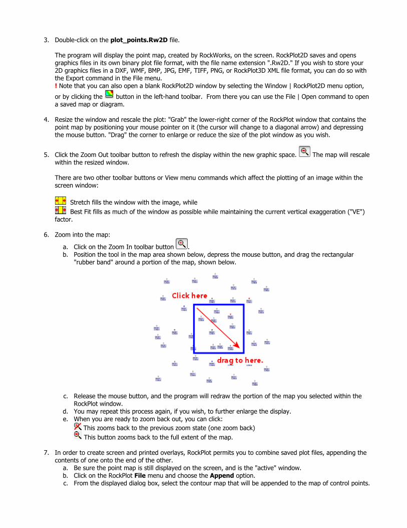
3. Double-click on the plot_points.Rw2D file.
The program will display the point map, created by RockWorks, on the screen. RockPlot2D saves and opens graphics files in its own binary plot file format, with the file name extension ".Rw2D." If you wish to store your 2D graphics files in a DXF, WMF, BMP, JPG, EMF, TIFF, PNG, or RockPlot3D XML file format, you can do so with the Export command in the File menu.! Note that you can also open a blank RockPlot2D window by selecting the Window | RockPlot2D menu option,
or by clicking the button in the left-hand toolbar. From there you can use the File | Open command to open a saved map or diagram.
4. Resize the window and rescale the plot: "Grab" the lower-right corner of the RockPlot window that contains the point map by positioning your mouse pointer on it (the cursor will change to a diagonal arrow) and depressing the mouse button. "Drag" the corner to enlarge or reduce the size of the plot window as you wish.
5. Click the Zoom Out toolbar button to refresh the display within the new graphic space. The map will rescale within the resized window.
There are two other toolbar buttons or View menu commands which affect the plotting of an image within the screen window:
Stretch fills the window with the image, while Best Fit fills as much of the window as possible while maintaining the current vertical exaggeration ("VE")
factor.
6. Zoom into the map:
a. Click on the Zoom In toolbar button . b. Position the tool in the map area shown below, depress the mouse button, and drag the rectangular
"rubber band" around a portion of the map, shown below.
c. Release the mouse button, and the program will redraw the portion of the map you selected within the RockPlot window.
d. You may repeat this process again, if you wish, to further enlarge the display. e. When you are ready to zoom back out, you can click:
This zooms back to the previous zoom state (one zoom back) This button zooms back to the full extent of the map.
7. In order to create screen and printed overlays, RockPlot permits you to combine saved plot files, appending the contents of one onto the end of the other.
a. Be sure the point map is still displayed on the screen, and is the "active" window. b. Click on the RockPlot File menu and choose the Append option. c. From the displayed dialog box, select the contour map that will be appended to the map of control points.
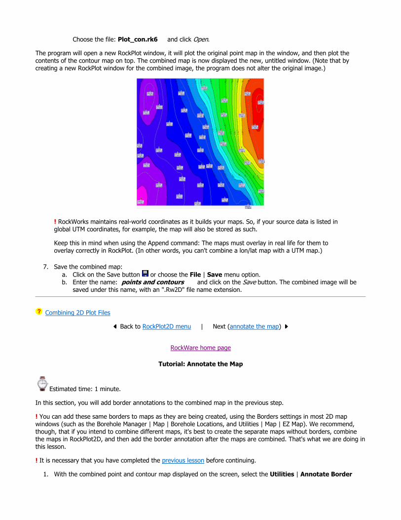
Choose the file: Plot_con.rk6 and click Open.
The program will open a new RockPlot window, it will plot the original point map in the window, and then plot the contents of the contour map on top. The combined map is now displayed the new, untitled window. (Note that by creating a new RockPlot window for the combined image, the program does not alter the original image.)
! RockWorks maintains real-world coordinates as it builds your maps. So, if your source data is listed in global UTM coordinates, for example, the map will also be stored as such.
Keep this in mind when using the Append command: The maps must overlay in real life for them to overlay correctly in RockPlot. (In other words, you can't combine a lon/lat map with a UTM map.)
7. Save the combined map: a. Click on the Save button or choose the File | Save menu option. b. Enter the name: points and contours and click on the Save button. The combined image will be
saved under this name, with an ".Rw2D" file name extension.
Combining 2D Plot Files
Back to RockPlot2D menu | Next (annotate the map)
RockWare home page
Tutorial: Annotate the Map
Estimated time: 1 minute.
In this section, you will add border annotations to the combined map in the previous step.
! You can add these same borders to maps as they are being created, using the Borders settings in most 2D map windows (such as the Borehole Manager | Map | Borehole Locations, and Utilities | Map | EZ Map). We recommend, though, that if you intend to combine different maps, it's best to create the separate maps without borders, combine the maps in RockPlot2D, and then add the border annotation after the maps are combined. That's what we are doing in this lesson.
! It is necessary that you have completed the previous lesson before continuing.
1. With the combined point and contour map displayed on the screen, select the Utilities | Annotate Border

menu command. 2. Adjust the settings:
a. Axes & Titles: Be sure the North, South, East, and West axes and their titles are all enabled (checked). b. Axis Titles: You can edit any titles as you wish. c. Border Dimensions: Find this setting at the lower-left corner of the window, and set this to Automatic.
3. Choose OK when you are through entering this information.
The program will add the requested annotation to the combined map, displayed in a new RockPlot window.
4. Save the map: a. Click on the Save button or choose the File | Save command to save this image. b. Type in the name: map with border and click the Save button. RockPlot will append the ".Rw2D" file
name extension automatically.
Annotating 2D Plot Files
Back to RockPlot2D menu | Next (measure distance)
RockWare home page
Tutorial: Measure Distances on the Map
Estimated time: 2 minutes.
In this section, you will use the Measure | Distance tool to record the distances between several boreholes on the combined, annotated map. This can be a helpful tool if you need to get an idea of your hole-to-hole distances prior to modeling, to better determine optimal grid/solid model node spacing (density).
! It is necessary that you have completed the previous lessons before continuing. Click here to return to the beginning of this section.
1. Enlarge the map: Maximize the RockPlot2D window that contains the combined, annotated map image, by clicking in the windows-maximize button.
2. Measure the distance: a. Click on the Measure menu and choose the Distance option. Or, click the Measure | Distance toolbar

button The program will display a bright message in the lower-right data pane, "Distance Calculator. Click on Starting Point."
b. Position the pointer on one of the borehole locations and left-click once. You’ll see a small symbol on top of the map symbol. The instructions in the data pane will now read, "Click on Ending Point."
c. Now position the pointer on another borehole location and left-click once. You’ll see a new symbol placed there, and a line will connect the two marked points.
d. The program will display the distance computation in the data pane of the plot window.
3. Repeat this for a few additional boreholes. Note how the distance measurements are posted there.
4. Save these measurements to a text file: a. Click on the Save button at the top of the data pane. b. In the displayed window, enter: distance.txt after the File Name prompt, and click the Save button.
The text file will contain all of the text in the data pane, and will be saved to the same folder as the current images. You could later open this text file in Windows Notepad, for example, to view the recorded data.
5. Refresh the image: Click on the Best Fit in Window button to redraw the map image. Note that the screen-digitized points and lines are now gone. The Distance measurements will still be displayed in the data pane, however.
! This is an important thing to note. The Measure menu items are only temporary in nature. Their markers will disappear from the image any time the screen is refreshed unless they are physically appended to the underlying image.
6. If you have a moment, experiment with some of the other Measure menu tools:Measure | Bearing: You digitize two points, and the program records the azimuth bearing (0 to 360 degrees) from the starting to the ending point.Measure | Perimeter: You digitize a polygon (double-click to close it) and the program records the perimeter length.Measure | Area: You digitize a polygon and the program records the area within the enclosed polygon.
Measuring the Distance Between Two Points
Back to RockPlot2D menu | Next (edit map)
RockWare home page
Tutorial: Edit the Map
Estimated time: 5 minutes.
In this section, you will use some of the RockPlot2D editing tools to make some changes to the map.
! It is necessary that you have completed the previous lessons before continuing. Click here to return to the beginning of this section.
1. With the annotated point and contour map still displayed on the screen, click on the Edit button in the RockPlot2D button palette.
2. Edit the upper scalebar title: a. Double-click on the scale bar along the top edge of the map You'll see the Scalebar Attributes window.

b. Title: Edit this text, which may default to "Easting" (unless you changed the text during the annotation step), to "Well Locations and Contours".
c. Color: Click in the Color box just to the right of the Title prompt, and select Blue. d. Click the Apply button to apply these changes. e. Click Close to close the window. You'll see the new title placed at the top of the map.
3. Edit one of the map symbols:
a. Click on the Zoom In button and click once or twice near any of the borehole location symbols to enlarge the view.
b. Click on the Edit button and then double-click on the symbol. c. Width, Height: Type in new values that are twice as large as the defaults. (Here, the size represents
actual map units.) For example, if the symbol is currently set to "4" for the width and height, you would change both values to "8".
d. Symbol: You can click on the picture of the symbol to select a different symbol design or color, clicking OK or Cancel to close the symbol selection window.
5. Click the Apply button to apply the editing changes. f. Click Close at the bottom of the Symbol Attributes window.
! Use the Undo command (Edit menu) to undo previous edits to the image. The File | Options menu item can adjust how many Undo levels will be available.
4. Edit the contour line vertices: a. Use the scroll bars along the bottom and right side of the display to scroll to the left or right, until you see
a labeled contour line. b. Click on the Edit button in the toolbar. c. Click on the contour line. When it's selected, you should see small handles on each vertex of the multi-
segmented line. d. Right-click on the selected line and choose Edit Vertices. You'll see the handles change color. e. Click on one of the blue-handled vertices and drag it to a new location. Release the mouse button to
complete the move. f. You can repeat this process for additional segments.
! Because this contour line is being smoothed, the vertex may not be placed exactly where you've defined. You can turn off line smoothing using the Properties window.
g. Click on the button at the bottom of the window (or press the Shift + Escape key) to get out of edit-vertex mode. The handles will return to the previous color.
h. Right-click on the still-selected contour line and choose Properties. i. Set the Smoothing to 0 and click OK.
The contour line will be redrawn with no smoothing.
5. Zoom back out by selecting the Zoom Out button .
6. Insert a raster image: a. Reposition the map window on your screen so that there is some white space to the right of the map. b. Select the Draw / Insert / Image menu item. c. Draw an insertion rectangle to the right of the map. You'll see a Raster (Bitmap) Attributes window.

d. Establish the image settings: Plot Border: Uncheck this.
Stretch: Uncheck this option. Load Image: Click this button. Select the file rp2dt_rockworks.png and click the Open button. Apply: Click the Apply button to insert the image into the map scene. Close: Click the Close button to close the Attributes window.
e. You'll see a logo now displayed to the right of the map. f. Click on the Edit button g. Click on the logo to select it. h. Drag to reposition the image, or click on one of the corner handles to resize it.
7. Save the changes to the map: Click the Save button or select the File | Save command. Don't close this window - you'll use it in the next lesson.
Back to RockPlot2D menu | Next (export map)
RockWare home page
Tutorial: Export the Map and Insert it into a Document
Estimated time: 2 minutes.
You may export any image displayed in a RockPlot2D window to a different graphic format for opening into another software program or inserting into document or report. The graphic exports that are available in RockPlot2D are BMP, JPG, KMZ (Google Earth), TIFF, PNG, DXF (AutoCAD Exchange Format), WMF (Windows Metafile), EMF (Enhanced Metafile), and RockPlot3D (Rw3D).
In this lesson, we will export the map from the previous lesson to a PNG format. The ".png" file will then be inserted into a document using your regular word processor.
! It is necessary that you have completed the previous lessons before continuing. Click here to return to the beginning of this section.
1. Be sure the combined, edited point + contour map is displayed in the active RockPlot window. This window should have the name "map with border.Rw2D." (If you need to re-open this map, go to the Project Manager pane along the left edge of the main RockWorks window, expand the 2-D Diagrams heading, and double-click on this map name.)
2. Select the File | Export command and select the PNG option from the pop-up menu.

The program will display a window where you can establish some size and resolution information.
3. Enter the requested information: a. Pixels per Inch: This sets the resolution for the bitmap, in numbers of dots or pixels per inch. Set the
resolution to: 300 by typing that value into the prompt box. b. Colors (bits per pixel): This determines the color "depth" of the output image. Be sure this is set to
Color (24b/p) for high color depth. c. Size in Inches, Scale (units per inch): Leave these as-is.
These settings permit you to export the image at a particular size in inches or at a particular X and Y scale in units per inch. If the Equal Scale box is checked (which would be appropriate for most RockWorks 2D maps and diagrams) any change to size or scale of one axis will update the other automatically, ensuring the width:height ratio remains the same.
d. Compression: Change this to Low. This causes the output file to be slightly bigger in size, but with less resolution loss.
4. Click OK at the bottom of the BMP Options window.
5. Enter a name for the PNG file. In the displayed prompt, the default name should be map with border.pngSimply click on the Save button to accept this name and perform the export.
6. Insert the map into a document. a. If you have a word processor of any kind installed on your computer, launch it at this time.
You can leave RockWorks running, with the map still displayed on the screen. If necessary, you can minimize both the RockPlot and RockWorks windows to access your word processor.
b. If necessary, create a new document in the word processor using its File | New command. (Some will launch and open a new file automatically.)
c. At the top of the new document, type in some introductory text, such as "This is my RockWorks map". Press the Enter key at the end of that line to advance to the next line in the document.
d. Now, you can insert the PNG version of the RockWorks map into the document. The instructions below correspond to the commands in Microsoft Word; if you are running a different program, you'll need to modify the selections accordingly.
e. In Microsoft Word click on the Insert menu and select Picture. (You may see a From File option; choose that.)
f. Browse to the RockWorks "Samples" folder, which is in your "My Documents\RockWorks16 Data" folder, and look for the file you just exported, named "map with border.png."
g. Click on that file name, and then click on the Insert button to insert the picture into the document.
Voila! The Bitmap version of your RockWorks map is now displayed in your report to your client.
7. Save: You may save the document using the word processor's File | Save command.
8. Close the word processor and return to RockWorks for the next lesson, exporting the map to RockPlot3D.
Exporting 2D Plot Files
Back to RockPlot2D menu | Next (export to Google Earth)
RockWare home page
Tutorial: Export the Map to Google Earth
Estimated time: 1 minute.
RockPlot2D contains a nifty tool for exporting map images to Google Earth, for display over your project area.
! It is necessary that you have completed the previous lessons before continuing. Click here to return to the beginning
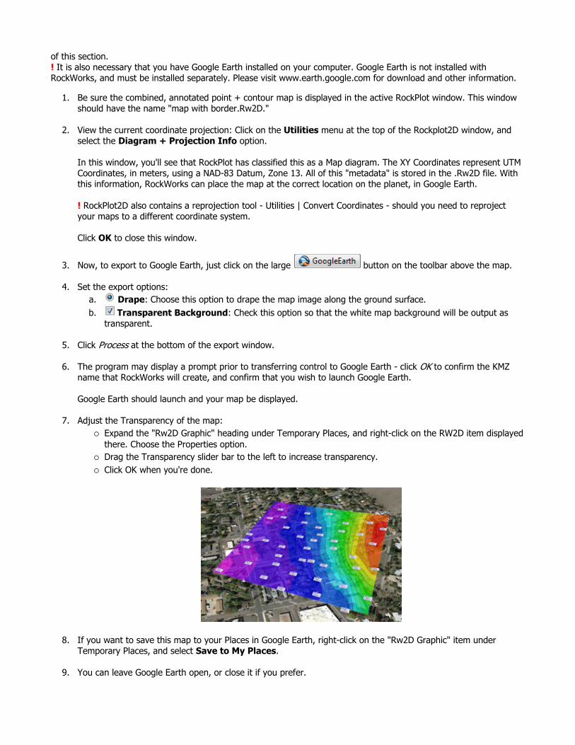
of this section.! It is also necessary that you have Google Earth installed on your computer. Google Earth is not installed with RockWorks, and must be installed separately. Please visit www.earth.google.com for download and other information.
1. Be sure the combined, annotated point + contour map is displayed in the active RockPlot window. This window should have the name "map with border.Rw2D."
2. View the current coordinate projection: Click on the Utilities menu at the top of the Rockplot2D window, and select the Diagram + Projection Info option.
In this window, you'll see that RockPlot has classified this as a Map diagram. The XY Coordinates represent UTM Coordinates, in meters, using a NAD-83 Datum, Zone 13. All of this "metadata" is stored in the .Rw2D file. With this information, RockWorks can place the map at the correct location on the planet, in Google Earth.
! RockPlot2D also contains a reprojection tool - Utilities | Convert Coordinates - should you need to reproject your maps to a different coordinate system.
Click OK to close this window.
3. Now, to export to Google Earth, just click on the large button on the toolbar above the map.
4. Set the export options: a. Drape: Choose this option to drape the map image along the ground surface. b. Transparent Background: Check this option so that the white map background will be output as
transparent.
5. Click Process at the bottom of the export window.
6. The program may display a prompt prior to transferring control to Google Earth - click OK to confirm the KMZ name that RockWorks will create, and confirm that you wish to launch Google Earth.
Google Earth should launch and your map be displayed.
7. Adjust the Transparency of the map: Expand the "Rw2D Graphic" heading under Temporary Places, and right-click on the RW2D item displayed there. Choose the Properties option. Drag the Transparency slider bar to the left to increase transparency. Click OK when you're done.
8. If you want to save this map to your Places in Google Earth, right-click on the "Rw2D Graphic" item under Temporary Places, and select Save to My Places.
9. You can leave Google Earth open, or close it if you prefer.

Exporting 2D Plot Files
Back to RockPlot2D menu | Next (print the map)
RockWare home page
Tutorial: Print the Map
Estimated time: 2 minutes.
You can output any image displayed in a RockPlot2D window to your printer that you have installed within Windows. There are three steps in this process: Be sure the file to be printed is displayed in the active RockPlot2D window, establish the printer settings, establish the printing scaling.
! The instructions given here will apply to maps as well as images such as ternary diagrams, Piper diagrams, scattergrams, etc.
1. Be sure the combined, annotated point + contour map is displayed in the active RockPlot2D window. This window should have the name "map with border.Rw2D."
a. If you can’t locate this window on your screen, hover over the RockWorks icon on the Windows taskbar. b. Click on the window with the RockPlot2D icon.
2. Set up the printer: Choose the Print Setup command from the RockPlot2D File menu. a. The program will display a standard Windows dialog box that lists the printers you have installed within
Windows, and the printer that is currently listed as default. For many printers, this window will also show the current paper size and orientation.
b. Choose a printer from this dialog box, if one is not already selected, for outputting the RockPlot2D map. c. For printing this map, be sure the paper, regardless of its size, is set to "Portrait" orientation. Check the
other settings for your printer to be sure they make sense for map plotting. d. Choose the OK button when you are ready to continue.
3. Now, let's set up for printing: a. Select the RockPlot2D File | Print command. The program will display a window for setting the plot
scaling. There are several portions of this dialog box to note; we will step you through them. b. Be sure to check out the diagram on the right side - this handy cartoon will let you know how your plot
will be placed on the printer paper based on current dialog box settings. Note also the Configure button at the top - this will bring up the settings available in the Print Setup dialog box you viewed earlier.
c. Horizontal Scale = Vertical Scale: The first step in printing is to check the Horizontal Scale = Vertical Scale setting. The status of this box will greatly affect how the rest of the settings behave. Be sure this box IS checked.
d. Units: Click on this tab, to the right. Choose whether your scaling units and margins are to be expressed as inches or centimeters.
e. Margins: Next, click on the Margins tab. You may override the displayed margins as necessary. They are expressed in decimal inches or centimeters as selected above. Note that these margins are in addition to any built-in printer margins (printers cannot generally print to the paper edges).
f. Layout Preview: Click back on this tab. g. Fill Page: If you have changed the margins, click on the Fill Page button at the top to re-dimension the
map with the new margin settings. h. Center: Next, click on the Center button (at the top) to re-center the map on the page. At equal scaling
x and y, you can toggle between centered and not-centered using the Fill Page and Center buttons. The change will be reflected in the cartoon.
The current output scale will be displayed near the middle of the screen. For example, "1 inch = 79.86163 units" indicates that each inch of the printed map will represent 79.86163 map units (meters, in this project). You can type in a different value if you prefer a rounded number, such as "80". As you change the scale, you can click the Center button again to re-center the map on the page.

4. That should do it for this map, so if you are ready to print, choose the Print button.
The program will send the map information to the printer. You may cancel at any time by choosing the Cancel button from the status window.
Printing RockPlot2D Images
Back to RockPlot2D menu
RockWare home page
Tutorial: Plot and Manipulate 3D Images - RockPlot3D
RockPlot3D is the 3D plotting window in RockWorks. It is used to display all 3-dimensional images generated by RockWorks, such as 3D logs, surfaces, solids, and fence diagrams. Whenever a diagram like this is created, it will be plotted automatically in a RockPlot3D tab in the Options window. RockPlot3D can also be displayed as a stand-alone window, not embedded in the program Options windows.
Since RockPlot3D is run as a separate application, outside RockWorks, all currently-open RockPlot3D windows can be seen in the Windows taskbar.
RockPlot3D contains many image manipulation features. The following lessons are offered:
If this is the first lesson set you’ve done, please be sure you’ve (1) opened a project folder, and (2) restored the program defaults.
Plot 3D logs (rotate, other views, dimensions, reference items, background color).
Append stratigraphic surfaces (adjust surface transparencies and other characteristics).
Add a stratigraphic legend.
Append a geochemical isosurface and airphoto (adjust isosurface appearance).
Export and zip the final scene.
! All of these lessons use existing 3D images, shipped with the program. See the Borehole Manager tutorial for other lessons regarding creating 3D images from downhole data, and manipulating them in RockPlot3D.
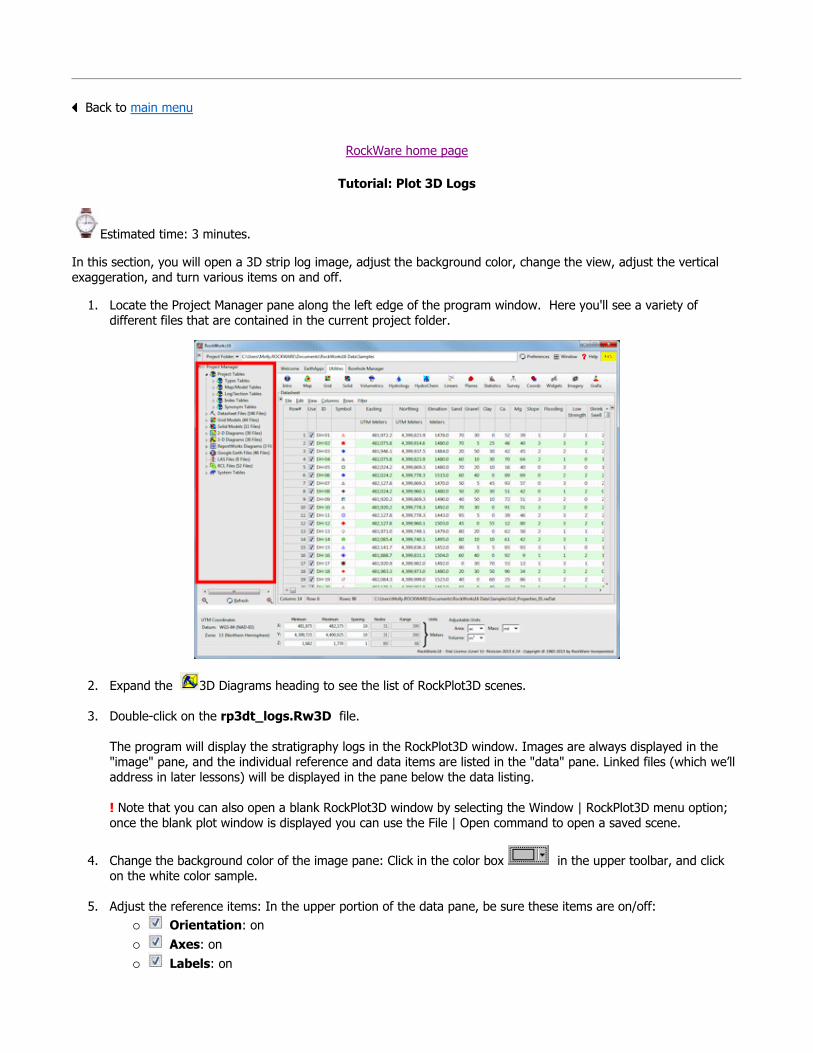
Back to main menu
RockWare home page
Tutorial: Plot 3D Logs
Estimated time: 3 minutes.
In this section, you will open a 3D strip log image, adjust the background color, change the view, adjust the vertical exaggeration, and turn various items on and off.
1. Locate the Project Manager pane along the left edge of the program window. Here you'll see a variety of different files that are contained in the current project folder.
2. Expand the 3D Diagrams heading to see the list of RockPlot3D scenes.
3. Double-click on the rp3dt_logs.Rw3D file.
The program will display the stratigraphy logs in the RockPlot3D window. Images are always displayed in the "image" pane, and the individual reference and data items are listed in the "data" pane. Linked files (which we’ll address in later lessons) will be displayed in the pane below the data listing.
! Note that you can also open a blank RockPlot3D window by selecting the Window | RockPlot3D menu option; once the blank plot window is displayed you can use the File | Open command to open a saved scene.
4. Change the background color of the image pane: Click in the color box in the upper toolbar, and click on the white color sample.
5. Adjust the reference items: In the upper portion of the data pane, be sure these items are on/off: Orientation: on Axes: on Labels: on

World Outline should not be checked.
6. Set the view to a pre-set location: Click on the RockPlot3D View menu and select the Above | South-Eastoption. The program will orient the display so that the logs are being viewed from above, from the southeast.
7. Rotate the image: The Rotate button should appear pressed in (it’s the default viewing tool). Position the mouse pointer in the middle of the image display, click and hold the mouse button, and drag slightly to the right. You should see the image rotate to the right. Release the mouse button to let go of the image. (If you want to take a moment to play with the rotation tool, feel free. You can always use the View | Above | South-Eastoption to reset the view.)
8. Adjust the Zoom: Click on the Zoom In toolbar button, and click anywhere in the scene to zoom into the view. You can also use the Zoom Percent drop-down at the top of the window, to enlarge the scene.
9. Save a Viewpoint: Once you have a viewing point and zoom state that you like, let's save this for later retrieval. Click on the View menu and choose Add View. Type in a name for this viewpoint, such as "Northwest Zoomed In" or "Overhead", and click OK. You'll see this displayed under the saved Views in the data tree.
To re-display the current 3D scene at that viewpoint, just double-click on it.
10. Adjust the vertical exaggeration: a. Click on the Dimensions button . This window displays the real-world coordinates of the 3D image. It
also controls the vertical stretch. b. Vertical Exaggeration: In this prompt, type in 1.5. c. Click the Apply button to make the changes take effect.
You should see the logs in the image pane appear stretched. There will be a note along the bottom of the RockPlot3D scene now, that "Vert Exag = 1.50".
11. In the data listing, you’ll see "groups" noted with the icon. This means that there are sub-items grouped together underneath the heading, visible if you expand the group’s "+" button.
a. Expand the "Logs" group heading in the data pane, and you’ll see the individual borehole names displayed. Remove the check-mark from the boring named "DH-12" and notice it has disappeared from the image pane. Re-activate the log by re-inserting its check-mark.
b. Expand the borehole group named "DH-4" and you’ll see the individual visible components to the log –the title and the stratigraphic layers. You can turn any of these items on and off by removing its check-
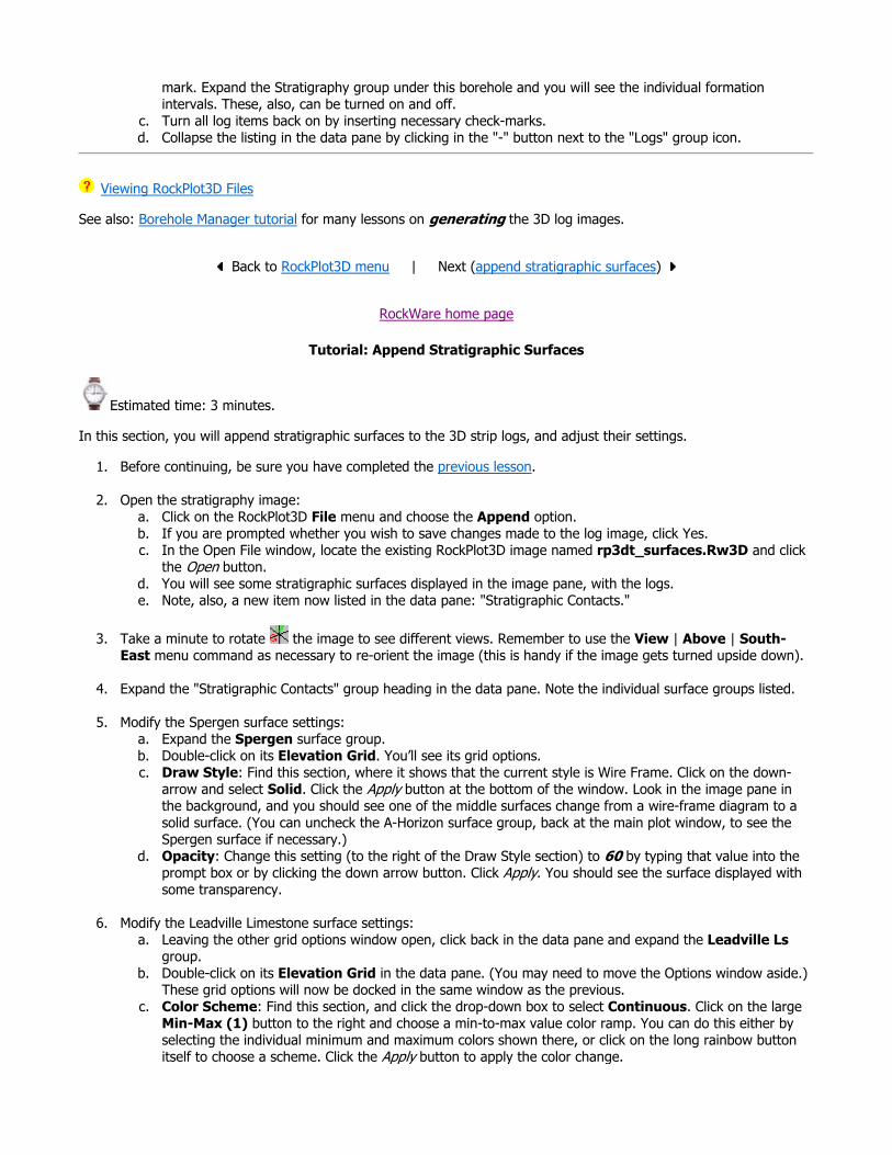
mark. Expand the Stratigraphy group under this borehole and you will see the individual formation intervals. These, also, can be turned on and off.
c. Turn all log items back on by inserting necessary check-marks. d. Collapse the listing in the data pane by clicking in the "-" button next to the "Logs" group icon.
Viewing RockPlot3D Files
See also: Borehole Manager tutorial for many lessons on generating the 3D log images.
Back to RockPlot3D menu | Next (append stratigraphic surfaces)
RockWare home page
Tutorial: Append Stratigraphic Surfaces
Estimated time: 3 minutes.
In this section, you will append stratigraphic surfaces to the 3D strip logs, and adjust their settings.
1. Before continuing, be sure you have completed the previous lesson.
2. Open the stratigraphy image: a. Click on the RockPlot3D File menu and choose the Append option. b. If you are prompted whether you wish to save changes made to the log image, click Yes. c. In the Open File window, locate the existing RockPlot3D image named rp3dt_surfaces.Rw3D and click
the Open button. d. You will see some stratigraphic surfaces displayed in the image pane, with the logs. e. Note, also, a new item now listed in the data pane: "Stratigraphic Contacts."
3. Take a minute to rotate the image to see different views. Remember to use the View | Above | South-East menu command as necessary to re-orient the image (this is handy if the image gets turned upside down).
4. Expand the "Stratigraphic Contacts" group heading in the data pane. Note the individual surface groups listed.
5. Modify the Spergen surface settings: a. Expand the Spergen surface group. b. Double-click on its Elevation Grid. You’ll see its grid options. c. Draw Style: Find this section, where it shows that the current style is Wire Frame. Click on the down-
arrow and select Solid. Click the Apply button at the bottom of the window. Look in the image pane in the background, and you should see one of the middle surfaces change from a wire-frame diagram to a solid surface. (You can uncheck the A-Horizon surface group, back at the main plot window, to see the Spergen surface if necessary.)
d. Opacity: Change this setting (to the right of the Draw Style section) to 60 by typing that value into the prompt box or by clicking the down arrow button. Click Apply. You should see the surface displayed with some transparency.
6. Modify the Leadville Limestone surface settings: a. Leaving the other grid options window open, click back in the data pane and expand the Leadville Ls
group. b. Double-click on its Elevation Grid in the data pane. (You may need to move the Options window aside.)
These grid options will now be docked in the same window as the previous. c. Color Scheme: Find this section, and click the drop-down box to select Continuous. Click on the large
Min-Max (1) button to the right and choose a min-to-max value color ramp. You can do this either by selecting the individual minimum and maximum colors shown there, or click on the long rainbow button itself to choose a scheme. Click the Apply button to apply the color change.
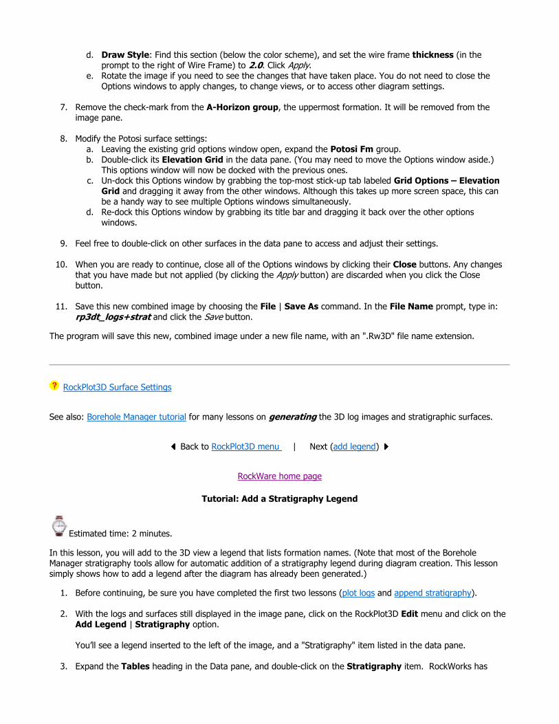
d. Draw Style: Find this section (below the color scheme), and set the wire frame thickness (in the prompt to the right of Wire Frame) to 2.0. Click Apply.
e. Rotate the image if you need to see the changes that have taken place. You do not need to close the Options windows to apply changes, to change views, or to access other diagram settings.
7. Remove the check-mark from the A-Horizon group, the uppermost formation. It will be removed from the image pane.
8. Modify the Potosi surface settings: a. Leaving the existing grid options window open, expand the Potosi Fm group. b. Double-click its Elevation Grid in the data pane. (You may need to move the Options window aside.)
This options window will now be docked with the previous ones. c. Un-dock this Options window by grabbing the top-most stick-up tab labeled Grid Options – Elevation
Grid and dragging it away from the other windows. Although this takes up more screen space, this can be a handy way to see multiple Options windows simultaneously.
d. Re-dock this Options window by grabbing its title bar and dragging it back over the other options windows.
9. Feel free to double-click on other surfaces in the data pane to access and adjust their settings.
10. When you are ready to continue, close all of the Options windows by clicking their Close buttons. Any changes that you have made but not applied (by clicking the Apply button) are discarded when you click the Close button.
11. Save this new combined image by choosing the File | Save As command. In the File Name prompt, type in: rp3dt_logs+strat and click the Save button.
The program will save this new, combined image under a new file name, with an ".Rw3D" file name extension.
RockPlot3D Surface Settings
See also: Borehole Manager tutorial for many lessons on generating the 3D log images and stratigraphic surfaces.
Back to RockPlot3D menu | Next (add legend)
RockWare home page
Tutorial: Add a Stratigraphy Legend
Estimated time: 2 minutes.
In this lesson, you will add to the 3D view a legend that lists formation names. (Note that most of the Borehole Manager stratigraphy tools allow for automatic addition of a stratigraphy legend during diagram creation. This lesson simply shows how to add a legend after the diagram has already been generated.)
1. Before continuing, be sure you have completed the first two lessons (plot logs and append stratigraphy).
2. With the logs and surfaces still displayed in the image pane, click on the RockPlot3D Edit menu and click on the Add Legend | Stratigraphy option.
You’ll see a legend inserted to the left of the image, and a "Stratigraphy" item listed in the data pane.
3. Expand the Tables heading in the Data pane, and double-click on the Stratigraphy item. RockWorks has

stored a copy of the stratigraphy library (called the Stratigraphy Types Table) in the RockPlot3D view. While you cannot edit the actual database using these tools, you can change what's displayed in the legend.
a. With the A-Horizon formation highlighted, along the left, remove the checkmark from the Show in Legend checkbox to the right.
b. Click on the Spergen Fm. formation name to the left. In the Caption prompt to the right, type in: Spergen Formation
c. Click OK at the bottom of the window.
4. Now, double-click on the Stratigraphy legend item in the data tree, to access its settings.
a. Change the font style/size: If the font looks big, click the Font button at the bottom of the Legend Options window and select a smaller font size. Choose a different font type if you want to. Once you close the font window, be sure to click Apply in the Legend Options window to apply the changes.
b. Legend location: You can play with putting the legend on the left or the right side of the image, clicking Apply any time you want a setting change applied. You can also adjust the horizontal and vertical offsets of the legend using the up or down arrows, using small increments.! The legends operate independently of the 3D image since they are placed in the "margin" of the View window. They are not enlarged if you zoom into the image, nor shrunk when you zoom out. They do not rotate or pan.
5. Click the Close button when you are ready to close the Legend Options window.
6. Save the changes: Select the File | Save command. The changes will be re-saved under the same file name.
RockPlot3D Legends
Back to RockPlot3D menu | Next (append isosurface)
RockWare home page
Tutorial: Append an Isosurface
Estimated time: 3 minutes.
In this lesson, you will add to the view an existing 3D scene that contains a solid model "isosurface" and a floating aerial image.
1. Before continuing, be sure you have completed at least the first two lessons (plot logs and append stratigraphy). Or, if you are rejoining this tutorial after a break, look for the RockPlot3D file rp3dt_logs+strat.Rw3D in the Project Manager pane. Double-click on it to open this view.
2. Append the solid model: a. With the logs and surfaces still displayed in the image pane, click on the RockPlot3D File menu and click
on the Append option. b. Locate the existing solid model image named rp3dt_benzene.Rw3D and click on that file name. Click
the Open button to open that file. (This file should reside in the "My Documents\Rockworks16 Data\Samples" folder.
c. You will see a block now displayed in the image pane, and a new data item "Benzene Isosurface" in the data pane.
d. You will also see an aerial photo above the surfaces, an "Aerial Photo" item in the data listing, and the actual image file name, "1955_Airphoto.png," displayed in the Linked File List to the lower-right.
3. Double-click on the Benzene Isosurface item in the data pane. The program will display the Isosurface Options window.
5. Adjust the isosurface filter. a. Locate the Iso-Level section in the middle of the window. The defaults show the minimum (left) and
maximum (right) values stored in the solid model. The current iso-level value should be set to 30. b. Into the Iso-Level Value prompt, type in: 5 and click the Apply button. This tells the program to display
those areas in the solid model with benzene concentrations greater than or equal to 5. You should see the image has changed, displaying a much larger isosurface.
c. Now type 50 into the isolevel prompt, and click Apply. Now you'll see a much smaller area with such high concentrations.
6. Remove the check-mark from the Logs group and/or the Stratigraphic Contacts group and/or the floating image in the data pane, to see the isosurface more clearly. Or, you can expand either of those groups to selectively remove logs and/or surfaces.
7. Rotate the image to see different views.
8. Use the Zoom In tool to click-and-drag an enlargement rectangle, to see a bigger view. You can rotate and pan the image while zoomed in.

9. Zoom back out just by clicking the Zoom Out button.
10. Save the current view: a. Select the File | Save As command. b. In the File Name prompt, type in: rp3dt_logs+strat+solid and click the Save button.
RockPlot3D will store this new, combined image under this new name, with an ".Rw3D" file name extension.
RockPlot3D Isosurface Settings
See also: Borehole Manager tutorial for many lessons on generating the 3D isosurfaces.
Back to RockPlot3D menu | Next (export & zip)
RockWare home page
Tutorial: Export and Zip the Final Image
Estimated time: 2 minutes.
In this lesson, you will export the RockPlot3D image to a JPG format, and you will create a ZIP file of the image and all of its linked files.
1. Before continuing, be sure you have completed the previous lesson, and you have displayed in the RockPlot3D window the image with 3D logs, stratigraphic surfaces, isosurface, and airphoto.
2. Establish a good export view: The RockPlot3D export is based on the current screen display. a. Rotate the image to a good view – you might try using the View | Above | South-West option to get to
that pre-set view, and then rotate the image slightly up and to the right to get a good view in between the surfaces.
b. Maximize the RockPlot3D window (if it’s not already) by clicking in the Windows Maximize button in the upper-right corner. Drag the divider between the image and data pane to enlarge the image window as much as you can. The image should be rescaled automatically within the resized window.
c. Use the Zoom drop-down at the top of the screen to select (or type in) a zoom level at which the image fills the screen.

3. Click on the File menu and choose the Export option. From the pop-up menu, click on JPG.
4. Establish the JPG export Dimensions: a. The Width and Height prompts will default to the number of pixels currently occupied by the image on the
screen, at 96 pixels per inch. The larger your monitor and the larger the RockPlot3D window, the larger these numbers will be. The program allows you to adjust these pixels to increase or decrease the resolution of the output JPG bitmap.Now comes the decision… The appropriate image resolution to request in this export really depends on what you want to do with the image. For example, if you will be displaying the JPG image on a web page (i.e. primarily for screen display) you won’t need the same pixel density you might need for a high-resolution print image. (More )
b. Maintain Aspect Ratio: For this image, be sure this box is checked. This will keep the width-to-height ratio the same (the image won’t be stretched along either axis).
c. Width: In this prompt, type in 1000 d. Height: Click in this box and it will be updated automatically for the new resolution.
5. Compression: Set the Compression to Highest Quality by dragging that slider bar all the way to the right.
6. Assign the JPG file name: Click on the button to the right of the File Name prompt, and in the displayed window type in: rp3dt_logs+strat+solid.jpg and click the Save button.
7. Back at the Export JPEG window, click on the OK button to proceed with the export.
The program will create a JPG-format image of the RockPlot3D view, and store it on disk.
8. Use a program of your preference to view this image – you can use Windows Paint or any other program that’s capable of opening or inserting JPG images. If you find that this resolution is too low for your liking, all you need to do is to increase the Width and Height pixels in the export window.
Exporting from RockPlot3D
One final lesson. You’ll recall that the current RockPlot3D view contains a linked file: the "1955_airphoto.png" file that contains the image that floats in the current scene.
When you use the File | Save command to save the ".Rw3D" file, you save only the links to these files, not the information contained in the files themselves. Thus, if you were to email this file only to your co-workers, when they opened the file into RockPlot3D, they would see a warning that the program couldn’t find the linked image file.
For this reason, it’s REALLY IMPORTANT that you create a Zip-format file containing the .Rw3D file and all linked files if you want to distribute the image to co-workers, clean up your hard drive, etc. This will assure that views you like will be saved in a "package" and files won’t be lost.
Here’s how:
9. Back at the RockPlot3D window, with the image still displayed, click on the File menu and select the Zip All Linked Files option.
10. In the displayed window, type into the File Name prompt: rp3dt_logs+strat+solid.zip and click the Savebutton.

RockPlot3D will create a ZIP-format file containing the .Rw3D file and all linked files.
! RockPlot3D cannot open ZIP-format files. You will need to use a compression/decompression program (such as WinZip or similar) to decompress the .zip "package" into its component files for opening into RockPlot3D.
Zipping a RockPlot3D View
Back to RockPlot3D menu
RockWare home page
Tutorial: Laying Out a Report Page - ReportWorks
The ReportWorks program is a page layout program that’s shipped with RockWorks. It makes it very easy to create a printable page with RockPlot2D images, other graphic images, shapes, text, scale bars and more.
You can launch ReportWorks from the Windows Start menu as well as from inside RockWorks via the Window / ReportWorks menu item.
Choose a lesson by clicking on its " ".
If this is the first lesson set you’ve done, please be sure you’ve (1) opened a project folder, and (2) restored the program defaults.
Insert a Log Profile and a Map
Append an Existing RwRpt File
Insert a Bitmap Image
Print the Page

Back to main tutorial menu
RockWare home page
Tutorial: Insert a Log Profile and a Map
Estimated time: 3 minutes.
If you completed any of the log cross-section lessons in the Borehole Manager section of the tutorial, you can use the ReportWorks program to lay out the sections on a page for printing or inclusion in a report. It’s assumed that you’ve saved the log diagram and the map as RockPlot2D files (.Rw2D).
! If you have not completed those lessons, that’s ok – we’ve included some sample images for you to work with.
1. Open a new ReportWorks window: From the main RockWorks menu, select Window | ReportWorks or click
on the ReportWorks button on the Welcome program tab .
2. Set up the page layout: a. Select the ReportWorks File | Print Setup option. You'll see the dimensions of your current printer
page. b. Click on the Printer: Select & Set button to view your printer name and options. c. Choose Landscape paper orientation. The options that you’ll see are dependant upon the printer you
have on your system. d. Click OK to close the Print Setup window. e. The Page Size settings should correspond with your paper size and layout. f. Click OK to close the Page Setup window. g. Use the View | Fit to Page command if you want to see the entire page in the current window.
3. Insert the log section diagram: a. Click on the RockPlot button or choose Tools | RockPlot (Rw2D). b. Draw a rectangular area below the profile by defining a square area as shown here:
The program will display a window where you’ll select the .Rw2D file name and set scaling.
c. RockPlot (.Rw2D) Tab:File Name: Click the small open-file button at the upper prompt to browse for the log section you created.
In the Lithology lesson, the file would be: lith log section.Rw2D. In the Stratigraphy lesson, the file would be: straight strat section.Rw2D. In the I-Data lesson, the file would be: idata log section.Rw2D. In the T-Data lesson, the file would be: toluene log section 2-14-07.Rw2DIn the P-Data lesson, the file would be: pdata log section.Rw2D. If you haven’t done any of those lessons, you can select the factory-installed file:

rept_section.Rw2D. All of these files would be in the My Documents\RockWorks15 Data\Samples folder.
Link: Click on this radio button. With this setting, ReportWorks will not store the contents of the cross section in its file. It will instead store the name of the section’s RK.Rw2D6 file and path and then read that external file into the page. See the ReportWorks Help messages for the pros and cons of linking versus embedding. Scaling: Choose Best Fit. This tells ReportWorks to keep the horizontal (section distance) and vertical (section elevation) scales equal. For your reference the scales that are represented are displayed in the Current View portion of the window, to the right.
d. Outline Tab: Click the Outline tab, displayed behind the RockPlot (*.Rw2D) tab. Style: Choose None by clicking the down-arrow button.
e. Fill (Background) Tab: Click on this tab to set the background appearance. Stock Fills: Be sure this option is selected, with the Style to None (for no fill).
f. Click the Apply button at the bottom of the window, and you’ll now see your log profile displayed on the page.
g. Click the Close button to close the dialog box. h. Feel free to adjust the profile’s position on the layout sheet by clicking and dragging it.
4. Insert the log profile map:
a. Click on the RockPlot button or choose Tools | RockPlot (Rw2D). b. Draw a rectangular area on the blank page by clicking and holding the mouse cursor in the upper-left
corner of the page and dragging down and to the right. Release the mouse button when you’ve got an area drawn line this:
c. RockPlot (.rk6) Tab:File Name: Like before, click the small open-file button at the upper prompt to browse for the map you saved, probably named log section map.Rw2D. If you did not complete any of the profile tutorials, you can browse for the factory-installed rept_map.Rw2D file.
All of these files would be in the My Documents\RockWorks16 Data\Samples folder. Link: Click on this radio button. As above, ReportWorks will read the image information from
the external file. Scaling: Choose Best Fit. As above, this sets the horizontal and vertical scales equal. For the map, unlike the profile, the horizontal and vertical axes both represent UTM map units.
d. Outline Tab: Click the Outline tab, displayed behind the RockPlot (*.Rw2D) tab. Style: Choose None by clicking the down-arrow button.
e. Fill (Background) Tab: Click on this tab to set the background appearance. Stock Fills: Be sure this option is selected, with the Style to None (for no fill).
f. Click the Apply button at the bottom of the window, and you’ll see your section map displayed on the page.
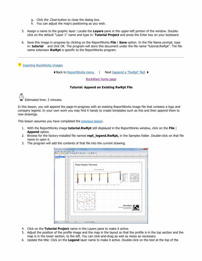
g. Click the Close button to close the dialog box. h. You can adjust the map’s positioning as you wish.
5. Assign a name to the graphic layer: Locate the Layers pane in the upper-left portion of the window. Double-click on the default "Layer 1" name and type in: Tutorial Project and press the Enter key on your keyboard.
6. Save this image in progress by clicking on the ReportWorks File | Save option. In the File Name prompt, type in: tutorial and click OK. The program will store this document under the file name "tutorial.RwRpt". The file name extension RwRpt is specific to the ReportWorks program.
Inserting RockWorks Images
Back to ReportWorks menu | Next (append a "RwRpt" file)
RockWare home page
Tutorial: Append an Existing RwRpt File
Estimated time: 2 minutes.
In this lesson, you will append the page-in-progress with an existing ReportWorks image file that contains a logo and company legend. In your own work you may find it handy to create templates such as this and then append them to new drawings.
This lesson assumes you have completed the previous lesson.
1. With the ReportWorks image tutorial.RwRpt still displayed in the ReportWorks window, click on the File | Append option.
2. Browse for the factory-installed file named rept_legend.RwRpt, in the Samples folder. Double-click on that file name to open it.
3. The program will add the contents of that file into the current drawing.
4. Click on the Tutorial Project name in the Layers pane to make it active. 5. Adjust the position of the profile image and the map in the layout so that the profile is in the top section and the
map is in the lower section, to the left. You can click-and-drag as well as resize as necessary. 6. Update the title: Click on the Legend layer name to make it active. Double-click on the text at the top of the

diagram that reads Place Project Title Here. In the displayed window, type in the following text: Tutorial Sample Data and click the Apply button. Click Close. The title will be updated as requested.
7. Save this updated layout using the File | Save command.
Back to ReportWorks menu | Next (insert bitmap)
RockWare home page
Tutorial: Add a Bitmap Image
Estimated time: 2 minutes.
In this lesson, you will add a BMP image to the drawing. This lesson assumes you have completed the previous lesson.
1. Click on the Tutorial Project layer name (upper-left) to make it active.
2. Click on the Raster (Bitmap) button or choose Tools | Raster (BMP, JPG, TIFF).
3. Draw a rectangular area to the right of the map by clicking and holding the mouse cursor in the upper-left corner of the page and dragging down and to the right. Release the mouse button when you’ve got an area drawn like the blue rectangle below:
The program will display a window where you’ll select the raster image file name and set scaling.
4. Raster Tab: a. Picture: Click the small open-file button at the upper prompt to browse for the sample file: 1955
Airphoto.png, and double-click on that file name. This file should reside in the My Documents\RockWorks16 Data\Samples folder.
b. Link: Click on the Link radio button c. Best Fit: Choose this option so that ReportWorks will keep the horizontal to vertical aspect ratio at
1:1 as you size the bitmap. d. Layer: This should default to the Tutorial Project layer.
5. Outline Tab: Click on this tab, displayed behind the Raster tab.

a. Style: Choose None by clicking the down-arrow button.
6. Click the Apply button at the bottom of the window, and you’ll now see the image displayed on the page.
7. Click the Close button to close the dialog box.
8. Adjust the image’s position on the layout sheet by clicking and dragging it. Remember that you can use the Layers to make different items active/inactive. Within the active layer, you can also use the right-click | Send to Back or Bring to Front options to adjust the stacking order.
9. Choose File | Save to save the layout thus far.
Inserting RockWorks Bitmaps
Back to ReportWorks menu | Next (print)
RockWare home page
Tutorial: Print the ReportWorks Page
Estimated time: 1 minute.
Let’s output this page to your printer. In order to continue, it’s assumed that you’ve completed the previous lesson.
1. With the Tutorial.RwRpt layout still displayed in the ReportWorks screen, click on the File | Print menu command.
You will see your printer’s Print dialog box.
2. Adjust any of the printing settings you like, using the Properties button.
3. Click the OK button to send the page to your printer.
Printing ReportWorks Documents
Back to ReportWorks menu
RockWare home page