tutorial - multiple-qtl mapping (mqm) analysis for r/qtltutorial - multiple-qtl mapping (mqm) ......

Tutorial - Multiple-QTL Mapping (MQM) Analysis for R/qtl

Danny Arends, Pjotr Prins, Karl W. Broman and Ritsert C. Jansen

October 27, 2014

1

1 Introduction

Multiple QTL Mapping (MQM) provides a sensitive approach for mapping quantititive traitloci (QTL) in experimental populations. MQM adds higher statistical power compared to manyother methods. The theoretical framework of MQM was introduced and explored by RitsertJansen, explained in the ‘Handbook of Statistical Genetics’ (see references), and used effectivelyin practical research, with the commercial ‘mapqtl’ software package. Here we present thefirst free and open source implementation of MQM, with extra features like high performanceparallelization on multi-CPU computers, new plots and significance testing.

MQM is an automatic three-stage procedure in which, in the first stage, missing data is‘augmented’. In other words, rather than guessing one likely genotype, multiple genotypes aremodeled with their estimated probabilities. In the second stage important markers are selectedby multiple regression and backward elimination. In the third stage a QTL is moved along thechromosomes using these pre-selected markers as cofactors, except for the markers in the windowaround the interval under study. QTL are (interval) mapped using the most ‘informative’ modelthrough maximum likelihood. A refined and automated procedure for cases with large numbersof marker cofactors is included. The method internally controls false discovery rates (FDR) andlets users test different QTL models by elimination of non-significant cofactors.

R/qtl-MQM has the following advantages:

• Higher power, as long as the QTL explain a reasonable amount of variation

• Protection against overfitting, because it fixes the residual variance from the full model.For this reason more parameters (cofactors) can be used compared to, for example, CIM

• Prevention of ghost QTL (between two QTL in coupling phase)

• Detection of negating QTL (QTL in repulsion phase)

The current implementation of R/qtl-MQM has the following limitations: (1) MQM is lim-ited to experimental crosses F2, BC, and selfed RIL, (2) MQM does not treat sex chromosomesdifferently from autosomal chromosomes - though one can introduce sex as a cofactor. Fu-ture versions of R/qtl-MQM may improve on these points. Check the website and change log(http://www.rqtl.org/STATUS.txt) for updates.

Despite these limitations, MQM 1 is a valuable addition to the QTL mapper’s toolbox. It isable to deal with QTL in coupling phase and QTL in repulsion phase. MQM handles missingdata and has higher power to detect QTL (linked and unlinked) than other methods. R/qtl’sMQM is faster than other implementations and scales on multi-CPU systems and computerclusters. In this tutorial we will show you how to use MQM for QTL mapping.

MQM is an integral part of the free R/qtl package [2, 1, 3] for the R statistical language2.

2 A quick overview of MQM

These are the typical steps in an MQM QTL analysis:

1MQM should not be confused with composite interval mapping (CIM) [13, 14]. The advantage of MQM overCIM is reduction of type I error (a QTL is indicated at a location where there is no QTL present) and type IIerror (a QTL is not detected) for QTL detection [9].

2We assume the reader knows how to load his data into R using the R/qtl read.cross function; see also theR/qtl tutorials [1] and book [2].

2

• Load data into R

• Fill in missing data, using either mqmaugmentdata or fill.geno

• Unsupervised backward elimination to analyse cofactors, using mqmscan

• Optionally select cofactors at markers that are thought to influence QTL at, or near, thelocation

• Permutation or simulation analysis to get estimates of significance, using mqmpermutationor mqmscanfdr

Using maximum likelihood (ML), or restricted maximum likelihood (REML), the algorithmemploys a backward elimination strategy to identify QTL underlying the trait. The algorithmpasses through the following stages:

• Likelihood-based estimation of the full model using all cofactors

• Backward elimination of cofactors, followed by a genome scan for QTL

• If there are no cofactors defined, the backward elimination of cofactors is skipped and agenome scan for QTL is performed, testing each genetic (interval) location individually.In this case REML and ML will result in the same QTL profile because there is no fullmodel.

The results created during the genome scan and the QTL model are returned as an (ex-tended) R/qtl scanone object. Several special plotting routines are available for MQM results.

3 Data augmentation

In an ideal world all datasets would be complete (with the genotype for every individual atevery marker determined), however in the real world datasets are often incomplete. That is,genotype information is missing, or can have multiple plausible values. MQM automaticallyexpands the dataset by adding all potential variants and attaching a probability to each. Forexample, information is missing (unknown) at a marker location for one individual. Based onthe values of the neighbouring markers, and the (estimated) recombination rate, a probabilityis attached to all possible genotypes. With MQM all possible genotypes with a probabilityabove the parameter minprob are considered.

When encountering a missing marker genotype (possible genotypes A and B in a RIL),all possible genotypes at the missing location are created. Thus at the missing location two‘individuals’ are created in the augmentation step, one with genotype A, and one with genotypeB. A probability is attached to both augmented individuals. The combined probability of allmissing marker locations tells whether a genotype is likely, or unlikely, which allows for weightedanalysis later.

To see an example of missing data with an F2 intercross, we can visualize the genotypes ofthe individuals using geno.image. In Figure 1 there are 2% missing values in white. The othercolors are genotypes at a certain position, for a certain individual. Simulate an F2 dataset with2% missing genotypes as follows:

Simulate a dataset with missing data:

3

> library(qtl)

> data(map10)

> simcross <- sim.cross(map10, type="f2", n.ind=100, missing.prob=0.02)

and plot the genotype data using geno.image (Figure 1):

> geno.image(simcross)

Before going to the next step (the QTL genome scan), the data has to be completed (i.e. nomore missing data). There are two possibilities: use (1) the MQM data augmentation routinemqmaugment or (2) the imputation routine fill.geno. Augmentation tries to analyse all possiblegenotypes of interest by leaving them in the solution space. In contrast, the imputation methodselects the most likely genotype, and uses that single individual for further analysis.

The downside of augmentation is that the addition of many possible genotypes can exceedavailable computer memory. Currently, augmentation moves an individual to a second aug-mentation round when it has too many possible genotypes (above the maximum number ofaugmented individuals maxaugind). In this second augmentation round the user can specifywhat needs to be done with these individuals: (1) Only use the most likely genotype, (2) usemultiple imputation to create multiple possible genotypes (up to maxaugind) or (3) removethe original genotype/individual from the analysis. Note that you can opt to use fill.geno’simputation method on your dataset, instead of augmentation, when too many individuals aredropped because of missing data.

The function mqmaugment is specific to MQM and the recommended procedure3. In thistutorial we focus on MQM ’s augmentation. The function mqmaugment fills in missing genotypesfor us. For each missing genotype data, at a marker, it fills in all possible genotypes andcalculates the probability. When the total probability is higher than the minprob parameterthe augmented individual is stored in the new cross object, ready for QTL mapping.

The important parameters are: cross, pheno.col, maxaugind, minprob and verbose (seealso the mqmaugment help page). maxaugind sets the maximum number of augmented genotypesper individual in a dataset. The default of 82 allows six missing markers per individual in aBC, and four in an F2. As a result the user has to increase the maxaugind parameter whenthere are more missing markers.

The minprob parameter sets the minimum probability of a genotype for inclusion in theaugmented dataset. This genotype probability is calculated for every marker relative to the mostlikely genotype of this individual. Note that setting this value too low may result in moving alot of individuals to the second augmentation round as the maximum of augmented individuals(the parameter maxaugind) is quickly reached. Increasing minprob (towards a value of 1.0) cankeep individuals with more missing data inside the first augmentation round; a possible ruleof thumb may be to set minprob to the percentage of data missing. A value of minprob=1.0makes augmentation behave similar to fill.geno’s imputation method, though with differentresulting genotypes. Use verbose=TRUE to get more feedback on the augmentation routine andto check how many individuals are moved to the second stage, for imputation or removal4

To start with an example, first run mqmaugment with minprob=1.0 (Figure 2):

Plot augmented data using geno.image:

3Note that after augmentation the resulting object is no longer suitable for the use with other R/qtl mappingfunctions, like scanone and cim, because they can not account for duplicated or dropped individuals.

4Augmentation is not always suitable with a lot of missing data, like in the case of selective genotyped datasets(for example the mouse hyper dataset that comes with R/qtl); these will always be handled with minprob=1.0

(and a warning will be issued).

4

50 100 150

20

40

60

80

100

Markers

Indi

vidu

als

1 2 3 4 5 6 7 8 9 10 11 12 13 14 15 16 171819 XGenotype data

Figure 1: Genotype data for a simulated F2 intercross generated with sim.cross, with 100individuals and 2% missing data. White pixels indicate missing genotypes.

5

> # displays warning because MQM ignores the X chromosome in an F2

> augmentedcross <- mqmaugment(simcross, minprob=1.0)

Plot the genotype data as follows:

> geno.image(augmentedcross)

With a lower minprob, more augmented individuals are kept, and the resulting augmenteddataset will be larger. Adding (weighted) augmented individuals with all possible genotypestheoretically leads to a more accurate mapping when dealing with missing values [11]5.

Try augmentation with minprob=0.1 (Figure 3):

> augmentedcross <- mqmaugment(simcross, minprob=0.1)

Plot the genotype data:

> geno.image(augmentedcross)

AnmQTL dataset (multitrait), which contains 24 metabolite traits from a RIL populationof Arabidopsis thaliana, is now distributed with R/qtl (load the data with data(multitrait)).This is part of the Arabidopsis thaliana RIL selfing experiment with Landsberg erecta (Ler)and Cape Verde Islands (Cvi) with 162 individuals scored 117 markers [17]. The experimentconcerned empirical untargeted metabolomics using liquid chromatography time of flight massspectrometry (LC-QTOF MS). This uncovered many qualitative and quantitative differencesin metabolite accumulation between Arabidopsis thaliana accessions [16].

Simulate missing data by removing some genotype data (5%, 10% and 80%) from the crossobject:

> data(multitrait)

> msim5 <- simulatemissingdata(multitrait, 5)



Next use augmentation to fill in the missing genotypes; with more missing data increasethe minprob parameter. When the minprob parameter is set too low it is possible that anindividual cannot be augmented, and is moved to the second round of augmentation (see thedescription above).

> maug5 <- mqmaugment(msim5)

> maug10 <- mqmaugment(msim10, minprob=0.25)

> maug80 <- mqmaugment(msim80, minprob=0.80)

Taking the 10% missing set, we can try a lower minprob=0.001. The output below showsthat ten augmented individuals miss too many markers to be augmented. By using the impu-tation strategy these individuals are kept in the set with a single ‘most likely’ genotype.

Augment with an imputation strategy:

5Note again that the augmented dataset can only be used with pure MQM functions. MQM functionsrecognise expanded individuals as single entities. Other R/qtl functions, like scanone, assume the augmentedindividuals are real individuals.

6

50 100 150

20

40

60

80

100

Markers

Indi

vidu

als

1 2 3 4 5 6 7 8 9 10 11 12 13 14 15 16 17 1819Genotype data

Figure 2: Genotypes, as visualized with geno.image, of 100 filled individuals (mqmaugment withminprob=1.0. With missing data only a ‘most likely’ individual is used and no real expansionof the dataset takes place, with similar results as fill.geno’s imputation method).

7

50 100 150

100

200

300

Markers

Indi

vidu

als

1 2 3 4 5 6 7 8 9 10 11 12 13 14 15 16 17 1819Genotype data

Figure 3: Genotypes, as visualized with geno.image of the augmented genotypes of 100 in-dividuals. There are a total of 399 ‘expanded’ individuals in this plot, because MQM fills inmissing markers with all likely genotypes (an average expansion of 4 per individual).

8

> maug10minprob <- mqmaugment(msim10, minprob=0.001, verbose=TRUE)

INFO: Received a valid cross file type: riself .

INFO: Number of individuals: 162 .

INFO: Number of chr: 5 .

INFO: Number of markers: 117 .

INFO: VALGRIND MEMORY DEBUG BARRIERE TRIGGERED

INFO: Done with augmentation

# Unique individuals before augmentation:162

# Unique selected individuals:162

# Marker p individual:117

# Individuals after augmentation:3599

INFO: Data augmentation succesfull

INFO: DATA-Augmentation took: 11.283 seconds

> maug10minprobImpute <- mqmaugment(msim10, minprob=0.001, strategy="impute",

+ verbose=TRUE)

INFO: Received a valid cross file type: riself .

INFO: Number of individuals: 162 .

INFO: Number of chr: 5 .

INFO: Number of markers: 117 .

INFO: VALGRIND MEMORY DEBUG BARRIERE TRIGGERED

INFO: Done with augmentation

# Unique individuals before augmentation:162

# Unique selected individuals:162

# Marker p individual:117

# Individuals after augmentation:4814

INFO: Data augmentation succesfull

INFO: DATA-Augmentation took: 18.005 seconds

> # check how many individuals are expanded:

> nind(maug10minprob)

[1] 3599

> nind(maug10minprobImpute)

[1] 4814

Next, scan for QTL inside the cross objects with mqmscan and the single-QTL mappingfunction scanone (for reference). The effect of increasing the amount of missing data on QTLmapping, using default values, can be seen in Figure 4.

> mqm5 <- mqmscan(maug5)



> msim5 <- calc.genoprob(msim5)

> one5 <- scanone(msim5)





9

0

2

4

6

8

10

MQM missing data

Chromosome

LOD

X3.

Hyd

roxy

prop

yl

1 2 3 4 5

MQM 5%MQM 10%MQM 80%

0

2

4

6

8

10

12

5% missing

Chromosome

lod

1 2 3 4 5

scanoneMQM

0

2

4

6

8

10

12

10% missing

Chromosome

lod

1 2 3 4 5

scanoneMQM

01234567

80% missing

Chromosome

lod

1 2 3 4 5

scanoneMQM

Figure 4: Arabidopsis thaliana RIL mQTL dataset (multitrait) with 24 metabolites as phe-notypes [16]. Effect of missing data on mqmscan after augmentation (green=5%, blue=10%,red=80%) and scanone (black), after fill.geno imputation.

10

02468

1012

Chromosome

lod

1 2 3 4 5

scanoneMQM

Figure 5: Arabidopsis thaliana RIL mQTL dataset (multitrait) with 24 metabolites as pheno-types [16] comparing MQM (mqmscan in green) and single QTL mapping (scanone in black).MQM shows similar results as single QTL mapping, when used without augmentation (minprobis 1.0), and with default parameters.

4 Multiple-QTL Mapping (MQM)

The multitrait dataset, distributed with R/qtl, contains 24 metabolite traits from a RILpopulation of Arabidopsis thaliana[16] (see also section 3 and help(multitrait) in R).

Here we analyse the multitrait dataset using both scanone (single-QTL analysis) andmqmscan (Multiple-QTL Mapping). First augment the data using the mqmaugment functionwith minprob=1.0, to compare against scanone with imputation (see also section 3).

Scan for QTL with mqmscan, after filling missing data with mqmaugment minprob=1.0:

> data(multitrait)

> maug_min1 <- mqmaugment(multitrait, minprob=1.0)

> mqm_min1 <- mqmscan(maug_min1)

We compare mqmscan with scanone. For scanone one first calculates conditional QTLgenotype probabilities via calc.genoprob.

> mgenop <- calc.genoprob(multitrait, step=5)

> m_one <- scanone(mgenop)

Figure 5 shows that, without augmentation, the results from MQM are similar to scanone.

mqmscan after augmentation, without cofactor selection:

> maug <- mqmaugment(multitrait)

> mqm <- mqmscan(maug)

11

By default MQM introduces fictional markers, or ‘pseudo markers’, at fixed intervals. Apseudo marker has a name like c7.loc25, which is the pseudo marker at 25 cM on chromo-some 7. (Note that this reflects the standard naming used in R/qtl.) Each chromosome isdivided into evenly spaced pseudo markers, step.size cM apart. A LOD score for underlyingQTL is calculated at these pseudo markers. A small step.size allows for smoother profilescompared with a pure marker-based mapping approach. The real markers are listed betweenthe pseudo markers. In the result you can remove the pseudo markers by using the functionmqmextractmarkers, as follows:

> real_markers <- mqmextractmarkers(mqm)

For model selection in MQM, first supply the algorithm with an initial model. This initialmodel can be produced in two ways: by (1) building a model by hand (forward stepwise), or (2)by unsupervised backward elimination on a large number of markers (discussed in Section 5).

First build this initial model by hand using a forward stepwise approach. (Note that theautomated procedure is preferred, both for theoretical and practical reasons.) A model consistsof a set of markers we want to account for. We can start building the initial model by addingcofactors at markers with high LOD scores scored by using mqmscan with default values. Figure 5displayed a large QTL peak on chromosome 5 at 35 cM. So we account for that by setting acofactor at the marker nearest to the peak on chromosome 5 and running mqmscan again. (SeeFigures 6 and 7.)

Add marker GH.117C (chromosome 5, at 35 cM) as a cofactor:

> max(mqm)

chr pos (cM) LOD X3.Hydroxypropyl info LOD*info

c5.loc35 5 35 10.6 0.523 5.55

> find.marker(maug, chr=5, pos=35)

[1] "GH.117C"

> multitoset <- find.markerindex(maug, "GH.117C")

> setcofactors <- mqmsetcofactors(maug, cofactors=multitoset)

> mqm_co1 <- mqmscan(maug, setcofactors)

The function find.marker identifies the name of the marker closest to 35 cM. The func-tion find.markerindex translates the marker name into a cofactor number. The functionmqmsetcofactors sets up a cofactor list for use with mqmscan.

Plot the results of the genome scan after adding a single cofactor (Figure 6):

> par(mfrow = c(2,1))

> plot(mqmgetmodel(mqm_co1))

> plot(mqm_co1)

Plot the mqmscan results with scanone results as follows (Figure 7):

> plot(m_one, mqm_co1, col=c("black","green"), lty=1:2)

> legend("topleft", c("scanone","MQM"), col=c("black","green"), lwd=1)

12

120100

80604020

0

Chromosome

Loca

tion

(cM

)

1 2 3 4 5

Genetic map

GH.117C

0

5

10

15

Chromosome

LOD

X3.

Hyd

roxy

prop

yl

1 2 3 4 5

Figure 6: Arabidopsis thaliana RIL mQTL dataset (multitrait) with 24 metabolites as phe-notypes [16]. mqmscan after a cofactor is added at the top scoring marker of chromosome 5.During the analysis it is kept in the model.

13

0

5

10

15

Chromosome

lod

1 2 3 4 5

scanoneMQM

Figure 7: Arabidopsis thaliana RIL mQTL dataset (multitrait) with 24 metabolites as pheno-types [16] after introducing a cofactor on chromosome 5 (GH.117C). mqmscan (green, dashed)differs from scanone (black).

Figures 6 and 7 show the effect of setting a single marker as a cofactor related to the QTLon chromosome 5, followed by an MQM scan. The marker is not dropped and it passes initialthresholding to account for the cofactor.significance level. LOD scores are expected tochange slightly, because of variation already explained by the QTL on chromosome 5 (Figure 7).

Figure 7 shows the second peak on chromosome 4 at 10 cM increases. Add a cofac-tor to the model and check if the model with both cofactors changes the QTL. Combiningfind.markerindex with find.marker, adds the new cofactor to the cofactor already in mul-

titoset (see Figure 8):

> # summary(mqm_co1)

> multitoset <- c(multitoset, find.markerindex(maug, find.marker(maug,4,10)))

> setcofactors <- mqmsetcofactors(maug,cofactors=multitoset)

> mqm_co2 <- mqmscan(maug, setcofactors)

Plot after adding second cofactor on chromosome 4 at 10 cM:


> plot(mqmgetmodel(mqm_co2))

> plot(mqm_co1, mqm_co2, col=c("blue","green"), lty=1:2)

> legend("topleft", c("one cofactor","two cofactors"), col=c("blue","green"),

+ lwd=1)

Plot the results with 0, 1 and 2 cofactors as follows:

> plot(mqm, mqm_co1, mqm_co2, col=c("green","red","blue"), lty=1:3)

> legend("topleft", c("no cofactors","one cofactor","two cofactors"),

+ col=c("green","red","blue"), lwd=1)

14

120100

80604020

0

Chromosome

Loca

tion

(cM

)

1 2 3 4 5

Genetic map

GA1GH.117C

0

5

10

15

20

Chromosome

LOD

X3.

Hyd

roxy

prop

yl

1 2 3 4 5

one cofactortwo cofactors

Figure 8: Arabidopsis thaliana RIL mQTL dataset (multitrait) with 24 metabolites as phe-notypes [16] using an added cofactor on chromosome 5 (blue), versus two cofactors, using anadditional cofactor on chromosome 4 (green).

15

0

5

10

15

20

Chromosome

LOD

X3.

Hyd

roxy

prop

yl

1 2 3 4 5

no cofactorsone cofactortwo cofactors

Figure 9: Arabidopsis thaliana RIL mQTL dataset (multitrait) with 24 metabolites as pheno-types [16]. Comparison of MQM adding 0 (green), 1 (red) and 2 (blue) cofactor(s) (note thatadding more cofactors does not improve the two QTL model).

When using the functions mqmsetcofactors, or the automated mqmautocofactor (describedin the next section), the number of cofactors is compared against the number of individualsinside the cross object. If there is a danger of setting too many cofactors, an error message isshown.

MQM also verifies the cofactor.significance level specified by the user. In the examplethe marker on chromosome 1 was informative enough, and included into the model. This waya new initial model consisting of cofactors on chromosome 4 and 5 was created. This (forward)selection of cofactors can continue until there are no more informative markers.

Manually determining the markers to set a cofactor can be very time consuming in the caseof many QTL underlying a trait. It is also prone to overfitting. Furthermore, manual fittingis generally not feasible for a large number of traits. Fortunately MQM provides unsupervisedbackward elimination, which is described in the next section.

16

5 Unsupervised cofactor selection through backward elimina-tion

MQM provides unsupervised backward elimination on a large number of markers by selectingcofactors automatically. Normally the number of markers in a dataset is much larger than thenumber of individuals. MQM allows using any number of cofactors simultaneously. This canbe as low as 0 cofactors up to a maximum of the number of individuals minus 12 (Inds− 12),as described in the Handbook of Statistical Genetics[4].

The functions: “mqmsetcofactor” and “mqmautocofactors” both create lists of cofactorsthat can be used for backward elimination. mqmautocofactor accounts for the underlyingmarker density and is therefore suitable for datasets with few individuals. See Figure 11 for acomparison on the multitrait dataset, using the mqmsetcofactors function to set cofactorsevery 5th marker and mqmautocofactor to set 50 cofactors across the genome. After cofactorselection MQM analyses and drops the least informative cofactor from the model. This step isrepeated until a limited number of informative cofactors remain. When taking marker densityinto account, an extra cofactor is introduced on chromosome 1 (see Figure 11).

After unsupervised backward elimination mqmscan scans each chromosome using the modelwith the remaining set of cofactors. For example, starting with 50 cofactors using mqmautoco-

factor and mqmsetcofactors, map QTL for the various traits in multitrait, which contains24 metabolite traits from a RIL population of Arabidopsis thaliana as described in section3. The QTL LOD scores differ between MQM and single QTL mapping with scanone (seeFigures 12 and 13).

Unsupervised cofactor selection through backward elimination:

> autocofactors <- mqmautocofactors(maug, 50)

> mqm_auto <- mqmscan(maug, autocofactors)

> setcofactors <- mqmsetcofactors(maug, 5)

> mqm_backw <- mqmscan(maug, setcofactors)

Visual inspection of the initial models:


> mqmplot.cofactors(maug, autocofactors, justdots=TRUE)

> mqmplot.cofactors(maug, setcofactors, justdots=TRUE)

Plot results:


> plot(mqmgetmodel(mqm_backw))

> plot(mqmgetmodel(mqm_auto))


> plot(mqmgetmodel(mqm_backw))

> plot(mqm_backw)

The mqmgetmodel function returns the final model from the output of mqmscan. This modelcan be further investigated using the fitqtl and fitqtl routines from R/qtl. mqmgetmodel

17

120100

80604020

0

Chromosome

Loca

tion

(cM

)

1 2 3 4 5

Genetic map

120100

80604020

0

Chromosome

Loca

tion

(cM

)

1 2 3 4 5

Genetic map

Figure 10: Arabidopsis thaliana RIL mQTL dataset (multitrait) with 24 metabolites as pheno-types [16]. mqmsetcofactor after introducing cofactors at every fifth marker (top) and mqmau-

tocofactor automatic marker selection (bottom). Automatic selection takes the underlyingmarker density into consideration.

18

120100

80604020

0

Chromosome

Loca

tion

(cM

)

1 2 3 4 5

Genetic map

GA1GH.117C

120100

80604020

0

Chromosome

Loca

tion

(cM

)

1 2 3 4 5

Genetic map

GA1

GH.121L−Col

Figure 11: Arabidopsis thaliana RIL mQTL dataset (multitrait) with 24 metabolites as phe-notypes [16]. mqmsetcofactor after introducing cofactors at every fifth marker (top) and mq-

mautocofactor automatic marker selection (bottom). mqmautocofactor places an additionalcofactor at chromosome 1 (see also Figure 10). After backward elimination this extra markerremains informative.

19

120100

80604020

0

Chromosome

Loca

tion

(cM

)

1 2 3 4 5

Genetic map

GA1GH.117C

05

10152025

Chromosome

LOD

X3.

Hyd

roxy

prop

yl

1 2 3 4 5

Figure 12: Arabidopsis thaliana RIL mQTL dataset (multitrait) with 24 metabolites as pheno-types [16]. Unsupervised cofactor selection through backward elimination using mqmsetcofac-

tor after introducing cofactors at every fifth marker. QTL mapped for trait X3.Hydroxypropylon chromosome 4 and 5.

20

05

10152025

Chromosome

lod

1 2 3 4 5

scanoneMQM

Figure 13: Arabidopsis thaliana RIL mQTL dataset (multitrait) with 24 metabolites as pheno-types [16]. Compare QTL mapping of MQM after introducing cofactors at every fifth markerand unsupervised backward elimination of cofactors (green, dashed), and scanone (black).

can only be used after backward elimination produces a significant model. The resulting modelcan also be used to obtain the location and name of the significant cofactors.

Plot result of MQM, using unsupervised backward elimination, against that of scanone:

> plot(m_one, mqm_backw, col=c("black","green"), lty=1:2)


> plot(m_one, mqm_backw, col=c("black","green"), lty=1:2)


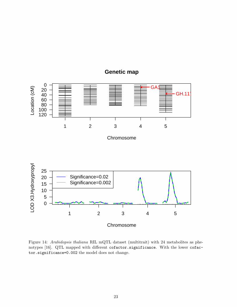
MQM QTL mapping may result in many significant (informative) cofactors. Figure 13shows at cofactor.significance=0.02 chromosomes 4 and 5 are involved. Lowering thesignificance level from 0.02 to 0.002 may yield a smaller model. In biology extensive modelsare sometimes preferred, but in general a simpler model is easier to understand and, perhaps,validated. Depending on the trait, and the sample size, increasing cofactor.significance canreduce the number of significant QTL in the model. In this example we have already have asmall model, so we don’t really expect to lose the two QTL on chromosome 4 and chromosome5. When decreasing the cofactor.significance no additional cofactors are dropped from themodel (See Figure 5)

21

Plot with lowered cofactor.significance:

> mqm_backw_low <- mqmscan(maug, setcofactors, cofactor.significance=0.002)


> plot(mqmgetmodel(mqm_backw_low))

> plot(mqm_backw,mqm_backw_low, col=c("blue","green"), lty=1:2)

> legend("topleft", c("Significance=0.02","Significance=0.002"),

+ col=c("blue","green"), lwd=1)

QTL mapped with different cofactor.significance=0.002, using the same starting mark-ers as Figure 12. As can be seen from the plot the models selected are similar. This means theQTL found significant at 0.02 are still significant at a more restrictive cutoff.:

When comparing the MQM scan in Figure 14 with the original scanone result in Figure 13there are some notable differences. Some QTL show higher significance (LOD scores) and someothers show lower significance and are, therefore, estimated to be less likely involved in thistrait.

Figures can be reconstructed from the result of mqmscan using the mqmplot.singletrait

function (see, for example, Figure 15). Here the model and QTL profile are retrieved. Thesefunctions can only be used with mqmscan functions, as they require the additional informationabout the inferred QTL model. The results also contain the estimated information content permarker.

> mqmplot.singletrait(mqm_backw_low, extended=TRUE)

The information content info in the result is calculated from the deviation of the ‘idealmarker distribution’. For example, with a dataset of 100 individuals, when comparing twodistinct phenotypes at a marker location, we have most power when both groups are equallydivided 50/50. A marker has virtually no power when one group containing 1 individual versusa group of 99. We can multiply the estimated QTL effect by this information content to‘clean’ the QTL profile by giving less weight to less informative markers. Please note that thesample size already plays a role in calculating QTL. Meanwhile it allows (informal) furtherweighting/exploring information content (Figure 15).

6 MQM effect plots

The function mqmplot.directedqtl is used to plot LOD curves with an indication of the signof the estimated QTL effects. This function because it uses internal R/qtl functions cannothandle augmented cross objects. An error will occur when the object supplied is augmentedusing mqmaugment. This requires using mqmscan with parameter outputmarkers=TRUE (default).

Create a directed QTL plot (Figure 16):

> dirresults <- mqmplot.directedqtl(multitrait, mqm_backw_low)

The results in Figure 14 imply that QTL on chromosomes 4 and 5 are associated with themetabolite X3.Hydroxypropyl. If we want to investigate the effects of the QTL, we can usethe functions plotPXG and effectplot. The following plots show these for markers GH.117C(main effect, Figure 17) and the interaction between GH.117C and GA1 (Figure 18).

The initial scans for X3.Hydroxypropyl (Figure 12) show two possible QTL on chromosome4 and 5. We can investigate interactions between these main effect QTL using the effectplot

22

120100

80604020

0

Chromosome

Loca

tion

(cM

)

1 2 3 4 5

Genetic map

GA1GH.117C

05

10152025

Chromosome

LOD

X3.

Hyd

roxy

prop

yl

1 2 3 4 5

Significance=0.02Significance=0.002

Figure 14: Arabidopsis thaliana RIL mQTL dataset (multitrait) with 24 metabolites as phe-notypes [16]. QTL mapped with different cofactor.significance. With the lower cofac-

tor.significance=0.002 the model does not change.

23

> mqmplot.singletrait(mqm_backw_low, extended=TRUE)

120100

80604020

0

Chromosome

Loca

tion

(cM

)

1 2 3 4 5

Genetic map

GA1GH.117C

05

10152025

Chromosome

QT

L (L

OD

)

1 2 3 4 5

Chromosome

QT

L (L

OD

)

1 2 3 4 5

0.00.20.40.60.81.0

LOD X3.HydroxypropylInformation Content

Figure 15: Arabidopsis thaliana RIL mQTL dataset (multitrait) with 24 metabolites as phe-notypes [16]. Plot using mqmplot.singletrait of the first metabolic trait. The informationcontent per marker (red) and the mapped QTL (black).

24

−25

−20

−15

−10

−5

0

Chromosome

LOD

X3.

Hyd

roxy

prop

yl

1 2 3 4 5

Figure 16: Arabidopsis thaliana RIL mQTL dataset (multitrait) with 24 metabolites as pheno-types [16]. Like Figure 15, but with LOD scores multiplied by ±1 according to the sign of theestimated QTL effect.

05000

100001500020000

Genotype

X3.

Hyd

roxy

prop

yl

GH.117C

AA BB

Figure 17: Arabidopsis thaliana RIL mQTL dataset (multitrait) with 24 metabolites as phe-notypes [16]. Main effect plot, with plotPXG, of marker GH.117C on trait X3.Hydroxypropyl.For each marker genotype the individual phenotype is plotted, with the mean of genotype AA(red) and BB (blue).

25

02000400060008000

1000012000

Interaction plot for GH.117C and GA1

GA1

X3.

Hyd

roxy

prop

yl

AA BB

AABB

GH.117C

Figure 18: Arabidopsis thaliana RIL mQTL dataset (multitrait) with 24 metabolites as phe-notypes [16]. Explore epistatic interaction, using effectplot, between markers GH.117C andGA1. GA1 appears to obscure the effect of GH.117C. An individual that has BB at GA1 hasno difference in expression between being AA or BB at GH.117C. However when an individualis AA at GA1 there is clear difference between the two genotype means ( 1.500 BB versus 12000when AA) at GH.117C.

function. To investigate the possible epistatic interaction, select markers GA1 (significant inFigure 12 and Figure 13) and GH.117C (significant in Figure 13 and 15). See Figure 18.

> effectplot(multitrait, mname1="GH.117C", mname2="GA1")

Likewise, in case we are interested in the interactions between the first small hump onchromosomes 1 (marker: PVV4 not significant) and the main efect on 5 (GH.117C), we couldmake interaction plots between these two markers with a high LOD score on those chromosomes.See Figure 19.

> effectplot(multitrait, mname1="PVV4", mname2="GH.117C")

Meanwhile, Figure 19 shows no evidence for an interaction between the two markers GH.117Cand PVV4, as the lines are close to parallel.

26

0

2000

4000

6000

8000

Interaction plot for PVV4 and GH.117C

GH.117C

X3.

Hyd

roxy

prop

yl

AA BB

AABB

PVV4

Figure 19: Arabidopsis thaliana RIL mQTL dataset (multitrait) with 24 metabolites as phe-notypes [16]. effectplot shows no epistatic effects between markers GH.117C and PVV4, thscan be seen because the two lines run in parallel, the genotype on one location (PVV4) doesnot affect the effect of the expression on GH.117C other location.

27

7 QTL significance

To estimate the significance of QTL and perhaps further exclude markers from a model, per-mutation testing is provided by the function mqmpermutation. This step is computationallyexpensive6 as the same test is repeated many times on shuffled data. Each test calculates LODscores for non associated (randomly ordered) data.

MQM provides parametric and non-parametric bootstrapping to estimate QTL significance.Select the type with the bootmethod parameter. If you have are lucky enough to have mul-tiple CPUs on your computer you can use the SNOW package [6, 5], which allows parallelcomputations on multiple CPU/cores.

SNOW is available through the Internet R archive CRAN. For example, with Rgui SNOWcan be installed by selecting from the menu: ‘Packages’ and ‘Install Package(s)‘ from the dropdown menu. Select a CRAN mirror near you and select the SNOW package. Rgui will startdownloading the package, and install any dependencies needed. Linux users can download acopy of SNOW from http://cran.r-project.org/web/packages/snow/index.html. Oncethe package has finished downloading the tar.gz file can be installed using R CMD INSTALL

snow.tar.gz

To summarize results from mqmpermutation, mqmprocespermutation makes the outputcomparable to scanone when using the n.perm parameter for permutation.

Calculate significance - using SNOW parallelization parameters:

> require(snow)

> results <- mqmpermutation(maug, scanfunction=mqmscan, cofactors=setcofactors,

+ n.cluster=2, n.perm=25, batchsize=25)

> resultsrqtl <- mqmprocesspermutation(results)

> summary(resultsrqtl)

LOD thresholds (25 permutations)

LOD X3.Hydroxypropyl

5% 2.16

10% 2.11

For small datasets, with a limited amount of classical traits, mqmpermutation is nice. How-ever, for large expression studies (eQTL) using microarrays, use mqmscanfdr instead, whichestimates false discovery rates (FDR) across the entire dataset at LOD cutoff, as described byBreitling et al.[18].

To estimate the FDR, mqmscanfdr permutes whole genome information, taking correlationbetween traits into account and giving an unbiased estimate of FDR at different (user specified)thresholds. The function scans the traits and counts observed QTL with a LOD above x,setting a certain threshold. It permutes all the data leaving the correlation structure betweentraits intact. Below, very high FDR estimates are calculated because of a small amount ofpermutations and high correlation between traits. We discover many QTL that map to thesame location. This can normally only happen with information sparse marker(s), or correlatedtraits, as seen in microarray experiments.

Calculate FDR:

6In the tutorial, for all examples, 25 permutations are used. A real experiment should use over 1000 permu-tation tests.

28

> mqmplot.permutations(results)

0 50 100 150 200

05

1015

2025

Markers

QT

L (L

OD

)

QTL trait# of bootstraps: 25

Figure 20: Arabidopsis thaliana RIL mQTL dataset (multitrait) with 24 metabolites as phe-notypes [16]. QTL significance calculated through permutation using mqmpermutation. Esti-mate by permuting a single trait (X3.Hydroxypropyl) with randomly distributing trait valuesamongst individuals, which gives an indication of LOD scores found by chance. QTL with aLOD higher than 2.5 can be considered significant (at cofactor.significance=0.05 (green)or cofactor.significance=0.10 (blue)). Chromosome are marked by the gray vertical gridlines.

29

> data(multitrait)

> m_imp <- fill.geno(multitrait)

> mqmscanfdr(m_imp, mqmscanall, cofactors=setcofactors, n.cluster=2)

above.in.real.res above.in.perm.res

1 1318 862.6 0.6544765

2 841 551.6 0.6558859

3 647 445.5 0.6885626

4 543 372.5 0.6860037

5 453 302.7 0.6682119

7 341 213.1 0.6249267

10 242 125.5 0.5185950

15 178 67.2 0.3775281

20 137 33.6 0.2452555

In contrast, the function mqmpermutation does single trait permutations, and does not takecorrelation between the traits into account. The advantage is that a permutation threshold isdetermined for each trait. This leads to different significance levels per trait and could leadto certain QTL being significant at their trait cut-off, which are not significant when a singlecut-off. The MQM output needs to be converted to the standard R/qtl format using themqmprocesspermutation function. The resulting object is of class scanoneperm and can beused by the standard R/qtl functions for further analysis.

To parallelize calculations n.cluster sets the number of CPU cores to use. A batch consistsof a number of traits to analyze on one core. A large(r) batchsize (default 10) can also be setto improve efficiency. Every time a batch is sent a new instance of R is started, so it pays tohave as few batches as possible.

8 Parallelized xQTL analysis

MQM can handle high throughput xQTL data - the name coined for the family of expressionQTL, or eQTL [7], metabolite QTL (mQTL) and pQTL (protein QTL), where measurementslike gene expression on microrray probes are treated as phenotypes. MQM analyses traits si-multaneously using parallel computing on multiple CPU/cores, and even computer clusters.xQTLdatasets (expression eQTL, metabolite mQTL) usually contain a large amount of pheno-types with known locations on the genome. These locations can be used for detecting cis/transregulation, for example. For QTL mapping every phenotype requires one or more calls tomqmscan. In addition special plots are presented for xQTLstudies.

Our example, the mQTL dataset multitrait, an Arabidopsis thaliana RIL cross, containing24 metabolites measured as phenotypes. Of these 24 phenotypes we will only scan the first fivephenotypes by setting the pheno.col parameter. To map back the regulatory locations of thesemetabolites one can use plain scanning of all metabolites (initially without cofactors). Next,we plot all the profiles in a heatmap (see Figure 21). In this heatmap the colors represent theLOD score, on the x-axis the marker number and on the y-axis the metabolite. The traits arenumbered in the plot. Plot heatmap without cofactors and then the heatmap with cofactors andbackward elimination. Figure 22 shows improvement over Figure 21 because of an improvedsignal to noise ratio.

> data(multitrait)

> m_imp <- fill.geno(multitrait)

> mqm_imp5 <- mqmscan(m_imp, pheno.col=1:5, n.cluster=2)

30

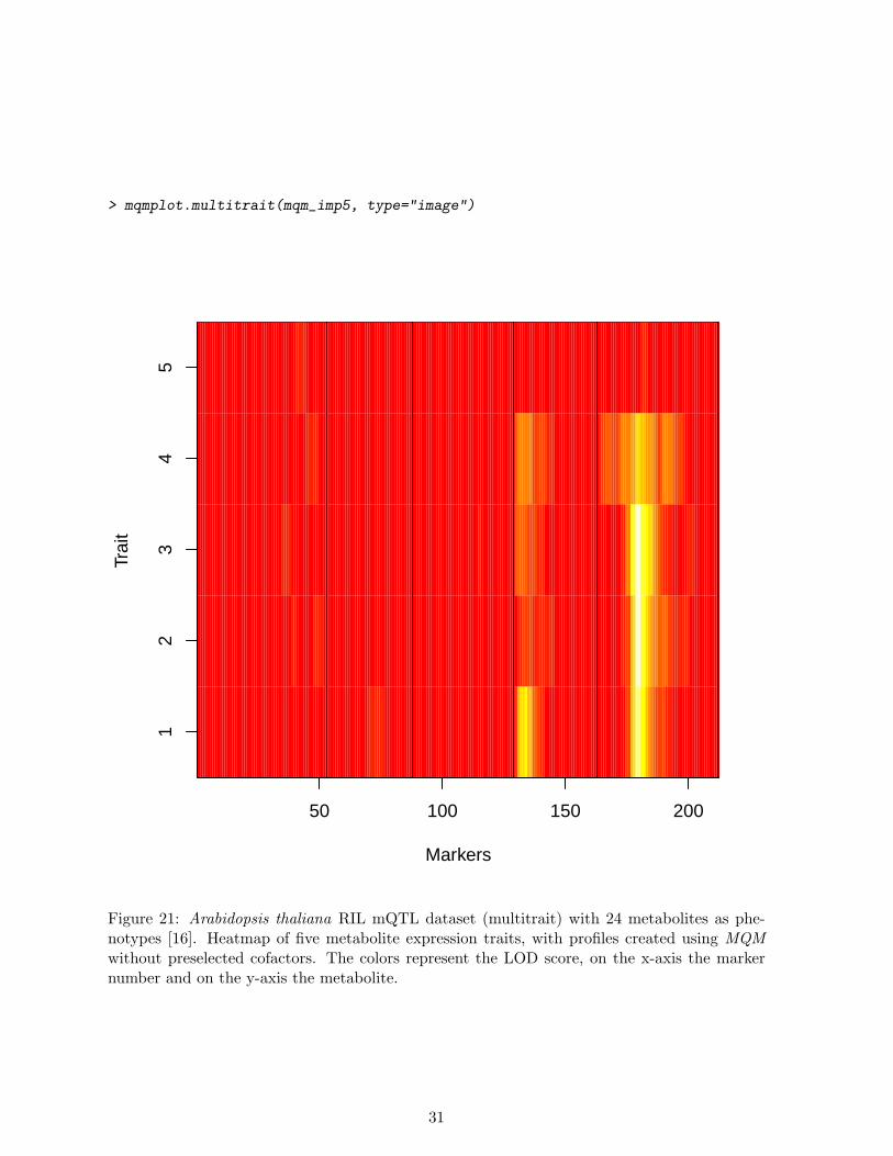
> mqmplot.multitrait(mqm_imp5, type="image")

50 100 150 200

12

34

5

Markers

Trai

t

Figure 21: Arabidopsis thaliana RIL mQTL dataset (multitrait) with 24 metabolites as phe-notypes [16]. Heatmap of five metabolite expression traits, with profiles created using MQMwithout preselected cofactors. The colors represent the LOD score, on the x-axis the markernumber and on the y-axis the metabolite.

31

> cofactorlist <- mqmsetcofactors(m_imp, 3)

> mqm_imp5 <- mqmscan(m_imp, pheno.col=1:5 , cofactors=cofactorlist,

+ n.cluster=2)

Use mqmplot.multitrait for more graphical output. (Unfortunately this does not show inthe generated PDF, but in R it shows the trait profiles)

> mqmplot.multitrait(mqm_imp5, type="lines")

Next is mqmplot.circle. The circle plot shows a circular representation of the genome.After using automatic backward selection certain marker/cofactors are found to be significant.These are highlighted and colored. The cofactor size can be scaled, based on significance (seeFigures 23 and 24).

The plot can be tweaked. For example, highlight a specific trait, and calculate interactionsbetween the significant cofactors. All other traits are grayed out, but remain partly visible, inthis way it is possible to see if significant QTL for this trait are also colocated with other traits.Parameter interactstrength: highlights interactions between significant markers. Howeverthey are only drawn (and reported in the output) if the effect change is larger than inter-

actstrength multiplied by the summed standard deviation. Parameter spacing sets spacebetween the chromosomes in Cm.

Next a cis-trans plot with mqmplot.cistrans. This plot is only available when genomiclocations of the traits are known, e.g. the genomic probe locations in microarray eQTL studies.By default the R/qtl cross object does not store this data. So the user has to add this informa-tion to the cross object using the addloctocross function. After this operation the cis-transplot can be created for QTL with associated genome locations.

The two axis of the cis-trans plot both show the genetic location. The X-axis is, normally,the QTL location and the Y-axis the locations of the trait.

When having locations we can, again, use the mqmplot.circle function, now with the extrainformation:

32

> mqmplot.multitrait(mqm_imp5, type="image")

50 100 150 200

12

34

5

Markers

Trai

t

Figure 22: Arabidopsis thaliana RIL mQTL dataset (multitrait) with 24 metabolites as phe-notypes [16]. Heatmap of metabolite expression traits, with profiles created using MQM withcofactors at each third marker. The colors represent the LOD score, on the x-axis the markernumber and on the y-axis the metabolite.

33

> mqmplot.circle(m_imp, mqm_imp5)

Distances in cM0 cM 19.6 cM39.2 cM

Chr 1


Chr 2


Chr 3Distances in cM

0 cM 19.6 cM39.2 cM

Chr 4


Chr 5

TraitQTL

Figure 23: Arabidopsis thaliana RIL mQTL dataset (multitrait) with 24 metabolites as pheno-types [16]. Circle plot 1 - Multiple metabolic traits without known locations. Four traits are inthe centre connected by a colored spline to their QTL. Significant QTL locations are depictedas solid square circles. A lower LOD score is closer to the center. A ’hotspot’ of QTL is visibleon chromosome 5.

34

> mqmplot.circle(m_imp, mqm_imp5, highlight=2)


Chr 1


Chr 2



0 cM 19.6 cM39.2 cM

Chr 4


Chr 5

Circleplot of: X4.Hydroxybutyl

TraitQTL

EC.66C

FD.111L−Col/136C

GA1

HH.159C−Col

DF.184L−Col

AD.129L−Col

Selected cofactor(s)Epistasis (+)Epistasis (−)

LOD 3LOD 6LOD 9LOD 12

Figure 24: Arabidopsis thaliana RIL mQTL dataset (multitrait) with 24 metabolites as phe-notypes [16]. Circle plot 2 - Multiple metabolic traits without known locations. Highlight thesecond trait. The significant QTL locations are depicted as solid red square circles. The splinesshow epistatic interactions (see also Figure 18). The blue lines are locations which are modu-lating expression (higher or lower), the green lines show a flip in effect. To explain this: withtwo markers, having AA at marker one shows trait mean AA > trait mean BB at marker twohowever when the individual has BB at marker one the effect at marker two is reversed AA <BB.

35

> data(locations)

> multiloc <- addloctocross(m_imp, locations)

> mqmplot.cistrans(mqm_imp5, multiloc, 5, FALSE, TRUE)

Cis/Trans QTL plot at LOD 5

Markers (in cM)

Loca

tion

of tr

aits

(in

cM

)

0 31 67 110 156 206 252 299 345 393 439 486

050

100

175

250

325

400

475

Figure 25: Arabidopsis thaliana RIL mQTL dataset (multitrait) with 24 metabolites as phe-notypes [16]. mqmplot.cistrans can be drawn when QTL have associated genome locations.QTL are plotted against the position on the genome they were measured (here mQTL for Ara-bidopsis thaliana), cutoff is at LOD=5. Normally these plots are created using 10.000 + traits.However because this tutorial is automatically generated we only use 5 traits to illustrate.

36

> mqmplot.circle(multiloc, mqm_imp5, highlight=2)


Chr 1


Chr 2



0 cM 19.6 cM39.2 cM

Chr 4


Chr 5

Circleplot of: X4.Hydroxybutyl

TraitQTL

EC.66C

FD.111L−Col/136C

GA1

HH.159C−Col

DF.184L−Col

AD.129L−Col

Selected cofactor(s)Epistasis (+)Epistasis (−)

LOD 3LOD 6LOD 9LOD 12

Figure 26: Arabidopsis thaliana RIL mQTL dataset (multitrait) with 24 metabolites as pheno-types [16]. Circle plot 3 - Multiple metabolic traits with known locations. Highlight the secondtrait. The significant QTL locations are depicted as solid red square circles. The known loca-tion of the trait is a red triangle. The splines show epistatic interactions (see also Figure 18).The blue lines are locations which are modulating expression (higher or lower), the green linesshow a flip in effect.

37

9 Overview of all MQM functions

Table 1: Added functionalitymqmaugment: data augmentationmqmscan: MQM modelling and scanningmqmsetcofactors: Set cofactors at markers (or at fixed locations)find.markerindex: Change marker numbering into mqmformatmqmscanall: mqmscanall scans all traits using MQMmqmpermutation: Single trait permutationmqmscanfdr: Genome wide False Discovery Rates (FDR)mqmprocesspermutation: Creates an R/qtl permutationobject

from the output of the mqmpermutation functionmqmplot.multitrait: plot multiple traits (MQMmulti object)mqmplot.directedqtl: plot of single trait with added QTL effectmqmplot.permutations: plot to show single trait permutationsmqmplot.singletrait: plot of single trait analysis with information contentmqmplot.circle: Genome plot of QTL in a circle (optional: Use of location information)mqmplot.cistrans: Genomewide plot of cis- and trans-QTL, above a thresholdaddloctocross: Adding genetic locations for traitsmqmtestnormal: Test normality of a trait

38

References

[1] Broman, K.W.; 2009 A brief tour of R/qtl. http://www.rqtl.org/tutorials/rqtltour.pdf.

[2] Broman, K. W.; Sen, S; 2009 A Guide to QTL Mapping with R/qtl. Springer.

[3] Broman, K.W.; Wu, H.; Sen, S.; Churchill, G.A.; 2003 R/qtl: QTL mapping in experimentalcrosses. Bioinformatics, 19:889–890.

[4] Jansen R. C.; 2007 Chapter 18 - Quantitative trait loci in inbred lines. Handbook of Statis-tical Genetics, 3rd edition. Wiley.

[5] Tierney, L.; Rossini, A.; Li, N.; and Sevcikova, H.; 2004 The snow Package: Simple Networkof Workstations. Version 0.2-1.

[6] Rossini, A.; Tierney, L.; and Li, N.; 2003 Simple parallel statistical computing. R. Universityof Washington Biostatistics working paper series, 193.

[7] Jansen R. C.; Nap J.P.; 2001 Genetical genomics: the added value from segregation. Trendsin Genetics, 17, 388–391.

[8] Jansen R. C.; Stam P.; 1994 High resolution of quantitative traits into multiple loci viainterval mapping. Genetics, 136, 1447–1455.

[9] Jansen R.C.; 1994 Controlling the Type I and Type II Errors in Mapping Quantitative TraitLoci. Genetics, Vol 138, 871–881.

[10] Churchill, G. A.; and Doerge, R. W.; 1994 Empirical threshold values for quantitative traitmapping. Genetics 138, 963–971.

[11] Jansen R. C.; 1993 Interval mapping of multiple quantitative trait loci. Genetics, 135, 205–211.

[12] Dempster, A. P.; Laird, N. M. and Rubin, D. B.; 1977 Maximum likelihood from incompletedata via the EM algorithm. J. Roy. Statist. Soc. B, 39, 1–38.

[13] Zeng, Z. B.; 1993 Theoretical basis for separation of multiple linked gene effects in mappingquantitative trait loci. Proc. Natl. Acad. Sci. USA, 90, 10972–10976.

[14] Zeng, Z. B.; 1994 Precision mapping of quantitative trait loci. Genetics, 136, 1457–1468

[15] Sugiyama, F.; Churchill, G.A.; Higgins, D.C.; Johns, C.; Makaritsis, K.P.; Gavras, H.;Paigen, B.; 2001 Concordance of murine quantitative trait loci for salt-induced hypertensionwith rat and human loci. Genomics, 71, 70–77.

[16] Keurentjes, J. J.; Fu, J.; de Vos, C. H.; Lommen, A.; Hall, R. D.; Bino, R. J.; van derPlas, L. H.; Jansen, R. C.; Vreugdenhil, D.; Koornneef, M.; 2006 The genetics of plantmetabolism. Nature Genetics. 38, 842–849.

[17] Alonso-Blanco, C.; Peeters, A. J.; Koornneef, M.; Lister, C.; Dean, C.; van den Bosch, N.;Pot, J.; Kuiper, M. T.; 1998 Development of an AFLP based linkage map of Ler, Col; CviArabidopsis thaliana ecotypes; construction of a Ler/Cvi recombinant inbred line population.Plant J. 14, 259–271.

[18] Breitling, R.; Li, Y.; Tesson, B. M.; Fu, J.; Wu, C.; Wiltshire, T.; Gerrits, A.; Bystrykh,L. V.; de Haan, G.; Su, A. I.; Jansen, R. C.; 2008 Genetical genomics: spotlight on QTLhotspots. PLoS Genet. 4/10.

39

tutorial - multiple-qtl mapping (mqm) analysis for r/qtltutorial - multiple-qtl mapping (mqm) ......

Documents