1

A few FAQs About QTL

Mapping

Guoyou Ye

E-mail: g.ye@cigar.org

Basics of QTL Mapping

What is QTL Mapping?

Map individual genetic factors on the quantitative traits,

to specific chromosomal segments in the genome.

The key questions in QTL mapping studies are:

� How many QTL are there?

� Where are they in the marker map?

� How large an influence does each of them have on

the trait of interest?

Dataset of QTL Mapping

� Mapping population

� Linkage map (can be constructed

using your own marker genotype

data)

� Marker genotype

� Phenotypic data

Mapping Population

� Biparental populations

� F2

� BC: backcross

� DH, doubled haploids

� RIL, recombination inbred lines

� CSSL: chromosome segment substitution

lines

� Natural population

Maximum Likelihood Method for

Estimating Recombination Rate

Recombination Rate

� Recombinant gametes: are derived by crossing over between the two parental gametes received by an individual.

� Recombination fraction: is the probability that gamete transmitted by an individual is recombinant.

Expected Marker Genotype Frequencies

BC1 BC2 DH Counts Expected Freq

M1M1M2M2 M1m1M2m2 M1M1M2M2 n1 f1= 21 (1－－－－r)

M1M1M2m2 M1m1m2m2 m1m1M2M2 n2 f2= 21 r

M1m1M2M2 m1m1M2m2 m1m1M2M2 n3 f3= 21 r

M1m1M2m2 m1m1m2m2 m1m1m2m2 n4 f4= 21 (1－－－－r)

Estimating Recombination Rate

� Likelihood function

� Logarithm operation of the likelihood function

� Maximum likelihood estimate

� Information: The negatives of the second derivatives

4321 )]1([][][)]1([!!!!

!21

21

21

21

4321

nnnnrrrr

nnnn

nL −−=

rnnrnnCL ln)()1ln()(lnln 3241 ++−++=

n

nn

nnnn

nnr 32

4321

32ˆ+

=+++

+=

)1(]

)1([)

ln(

2

32

2

41

2

2

rr

n

r

nn

r

nnE

rd

LdEI

−=

+−

−

+−−=−=

n

rr

IVr

)ˆ1(ˆ1ˆ

−==

Example

� BC experiment

� P1 and P2 are AABB and aabb, respectively

� Number of plants of different genotypes in the population

� AABB：162；AABb：40；AaBB：41；AaBb：158

%20.20401

81

1584140162

4140ˆ ==

+++

+=r

4

ˆ 1002.4)ˆ1(ˆ −

×≈−

=n

rrVr

Recombination Rate When Three

Markers Are Linked

�Whenδ=0 (Crossovers in the two intervals are

independent),

or

�when δ= 1 (Complete interference, crossover at on

interval completely prevent crossover event in the other

interval)

2312231213 )1(2 rrrrr δ−−+=

2312231213 )1)(1()1( rrrrr +−−=−

231223122312231213 2)1()1( rrrrrrrrr −+=−+−=

231213 rrr +=

Mapping Function

� Mapping distance

� Unit of mapping distance：Morgan (M）or centi-Morgan (cM）,

1M= 100 cM

� Morgan is defined as that distance along which one crossing over is

expected to occur per gamete per generation

� Mapping distance m is function of recombination rate：

� f is called mapping function

231213 mmm +=

)(rfm =

Common Mapping Functions

• Morgan

m =r ×100 (cM)

• Haldane: no interference

• Kosambi with interference

)1( 2

21 mer −

−=

r

rm

21

21ln25

−

+=

1

1

2

125/

25/

+

−=

ee

m

m

r

三种作图函数的比较

15

Basic Principle of QTLMapping

� Distribution of trait values of three marker genotypes of a maker

Maximum likelihood Estimation

� A common approach in statistical estimation

• Define hypotheses

• Generate likelihood function

• Estimate

• Test hypotheses

• Draw statistical conclusions

Hypotheses in Linkage Analysis

� H0:

� θ = 0.5

� the QTL is not linked to the marker(s)

� HA:

� θ ≠ 0.5

� the QTL is linked to the marker(s)

Expected Marker Genotype

Frequencies

BC1 BC2 DH Counts Expected Freq

M1M1M2M2 M1m1M2m2 M1M1M2M2 n1 f1= 21 (1－－－－r)

M1M1M2m2 M1m1m2m2 m1m1M2M2 n2 f2= 21 r

M1m1M2M2 m1m1M2m2 m1m1M2M2 n3 f3= 21 r

M1m1M2m2 m1m1m2m2 m1m1m2m2 n4 f4= 21 (1－－－－r)

QTL Effects and QTL Genotypic

Value

� The additive (a) and dominance (d) genetic model

� P1 (A1A1): m+a; F1 (A1A2): m+d; P2 (A2A2): m-a

� Code of the three genotypes at a locus: 2 (P1), 0 (P2), 1 (F1)

Genotype P2: A2A2 (0) F1: A1A2 (1) P1: A1A1 (2)

mid-parent m

Genotypic G22 G12 G11

value

Additive a Additive a

Dominance d20

Quiz 1：：：：What is LOD ？？？？

� LRT: likelihood ratio test

� LOD : (Likelihood of Odd)

� A LOD-score threshold of 3 corresponds to a single-test p-value of

approximately 0.0001

)ln(2 0

AL

LLRT −=

)log()log()log( 0

0

LLL

LLOD A

A−==

61.4)10ln(2

LRTLRTLOD ≈= LODLRT 61.4≈

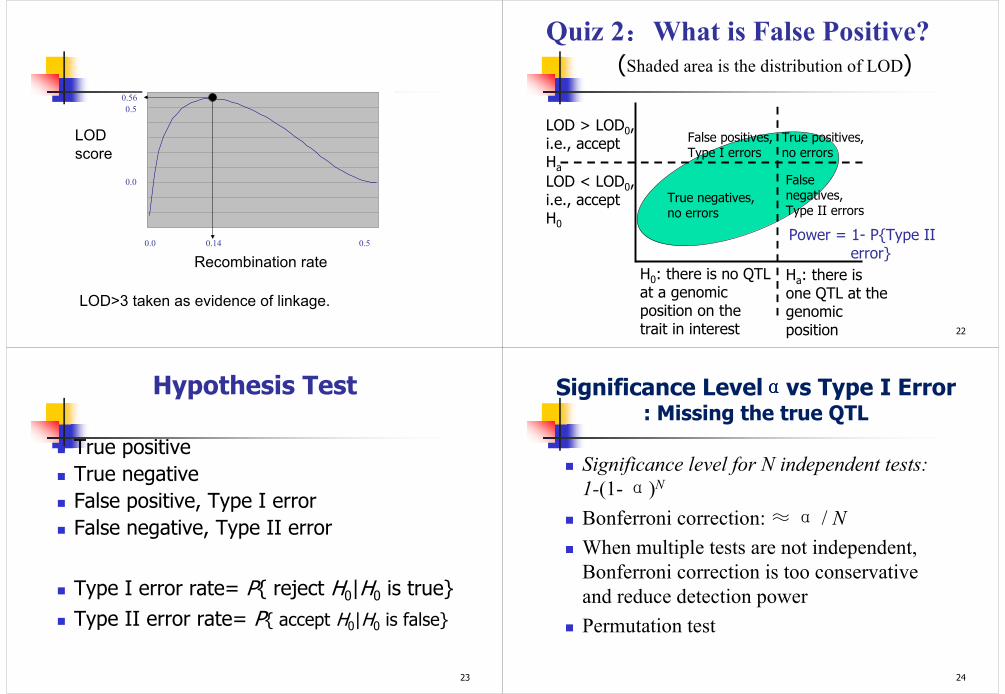
0.0 0.5

0.0

0.5

0.14

0.56

Recombination rate

LOD

score

LOD>3 taken as evidence of linkage.

22

Quiz 2：：：：What is False Positive?(Shaded area is the distribution of LOD)

H0: there is no QTL at a genomic position on the trait in interest

Ha: there is one QTL at the genomic position

LOD < LOD0, i.e., accept H0

LOD > LOD0, i.e., accept Ha

True negatives, no errors

True positives, no errors

False positives, Type I errors

False negatives, Type II errors

Power = 1- P{Type II error}

23

Hypothesis Test

� True positive

� True negative

� False positive, Type I error

� False negative, Type II error

� Type I error rate= P{ reject H0|H0 is true}

� Type II error rate= P{ accept H0|H0 is false}

Significance Levelααααvs Type I Error : Missing the true QTL

� Significance level for N independent tests:

1-(1- α)N

� Bonferroni correction: ≈α / N

� When multiple tests are not independent,

Bonferroni correction is too conservative

and reduce detection power

� Permutation test

24

25

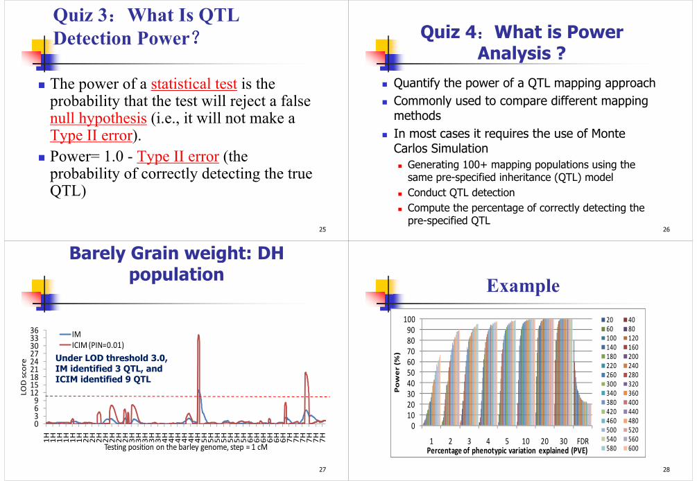
Quiz 3：：：：What Is QTL

Detection Power？？？？

� The power of a statistical test is the probability that the test will reject a false null hypothesis (i.e., it will not make a Type II error).

� Power= 1.0 - Type II error (the probability of correctly detecting the true QTL)

Quiz 4：：：：What is Power Analysis ?

� Quantify the power of a QTL mapping approach

� Commonly used to compare different mapping methods

� In most cases it requires the use of Monte Carlos Simulation

� Generating 100+ mapping populations using the same pre-specified inheritance (QTL) model

� Conduct QTL detection

� Compute the percentage of correctly detecting the pre-specified QTL

26

27

Barely Grain weight: DH population

0369

121518212427303336

1H

1H

1H

1H

1H

1H

2H

2H

2H

2H

2H

2H

2H

3H

3H

3H

3H

3H

4H

4H

4H

4H

4H

4H

5H

5H

5H

5H

5H

5H

5H

6H

6H

6H

6H

6H

6H

7H

7H

7H

7H

7H

7H

LO

D s

co

re

Testing position on the barley genome, step = 1 cM

IM

ICIM (PIN=0.01)

Under LOD threshold 3.0, IM identified 3 QTL, and ICIM identified 9 QTL

Example

28

0

10

20

30

40

50

60

70

80

90

100

1 2 3 4 5 10 20 30 FDR

Po

we

r (

%)

Percentage of phenotypic variation explained (PVE)

20 40

60 80

100 120

140 160

180 200

220 240

260 280

300 320

340 360

380 400

420 440

460 480

500 520

540 560

580 600

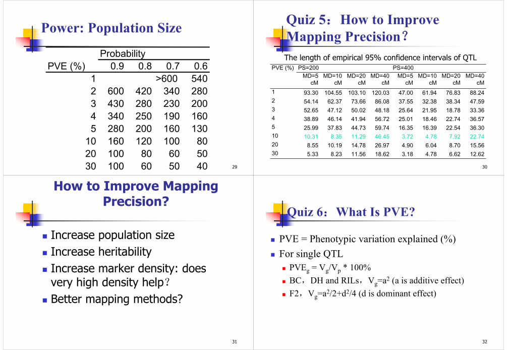
Power: Population Size

29

Probability

PVE (%) 0.9 0.8 0.7 0.6

1 >600 540

2 600 420 340 280

3 430 280 230 200

4 340 250 190 160

5 280 200 160 130

10 160 120 100 80

20 100 80 60 50

30 100 60 50 40

Quiz 5：：：：How to Improve

Mapping Precision？？？？

30

PVE (%) PS=200 PS=400MD=5

cMMD=10

cMMD=20

cMMD=40

cMMD=5

cMMD=10

cMMD=20

cMMD=40

cM1 93.30 104.55 103.10 120.03 47.00 61.94 76.83 88.242 54.14 62.37 73.66 86.08 37.55 32.38 38.34 47.593 52.65 47.12 50.02 48.18 25.64 21.95 18.78 33.364 38.89 46.14 41.94 56.72 25.01 18.46 22.74 36.575 25.99 37.83 44.73 59.74 16.35 16.39 22.54 36.3010 10.31 8.35 11.29 46.45 3.72 4.78 7.92 22.7420 8.55 10.19 14.78 26.97 4.90 6.04 8.70 15.5630 5.33 8.23 11.56 18.62 3.18 4.78 6.62 12.62

The length of empirical 95% confidence intervals of QTL

How to Improve Mapping Precision?

� Increase population size

� Increase heritability

� Increase marker density: does very high density help？

� Better mapping methods?

31 32

Quiz 6：：：：What Is PVE?

� PVE = Phenotypic variation explained (%)

� For single QTL

� PVEg = Vg/Vp * 100%

� BC，DH and RILs，Vg=a2 (a is additive effect)

� F2，Vg=a2/2+d2/4 (d is dominant effect)

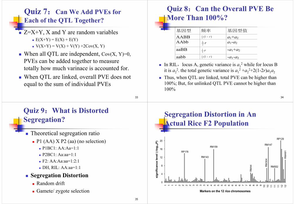
Quiz 7：：：：Can We Add PVEs for

Each of the QTL Together?

� Z=X+Y, X and Y are random variables

� E(X+Y) = E(X) + E(Y)

� V(X+Y) = V(X) + V(Y) +2Cov(X, Y)

� When all QTL are independent, Cov(X, Y)=0,

PVEs can be added together to measure

totally how much varinace is accounted for.

� When QTL are linked, overall PVE does not

equal to the sum of individual PVEs

33

Quiz 8：：：：Can the Overall PVE Be

More Than 100%?

� In RIL，locus A, genetic variance is a12 while for locus B

it is a22. the total genetic variance is a1

2 +a22+2(1-2r)a1a2

� Thus, when QTL are linked, total PVE can be higher than

100%; But, for unlinked QTL PVE cannot be higher than

100%

34

基因型 频率 基因型值

AABB )1(2

1 r− a1+a2

AAbb r2

1 a1-a2

aaBB r2

1 -a1+a2

aabb )1(2

1 r− -a1-a2

Quiz 9：：：：What is Distorted

Segregation?

� Theoretical segregation ratio

� P1 (AA) X P2 (aa) (no selection)

� P1BC1: AA:Aa=1:1

� P2BC1: Aa:aa=1:1

� F2: AA:Aa:aa=1:2:1

� DH, RIL: AA:aa=1:1

� Segregation Distortion

� Random drift

� Gamete/ zygote selection

35

Segregation Distortion in An

Actual Rice F2 Population

RP178

RM143

RM159

RM44 RM304

RM147

RM552

RP129

RM491

0

4

8

12

16

20

1 1 1 1 2 2 2 2 3 3 3 3 4 4 5 5 5 5 6 6 6 6 7 7 8 8 9 9

10

10

11

11

11

12

12

significance level (-log10P)

Markers on the 12 rice chromosomes

When Distorted Markers Are Not

Linked With QTLA

B

0

20

40

60

80

100

qPH1-1 qPH1-2 qPH3-1 qPH3-2 qPH4 qPH5 qPH6 qPH7 qPH12 FDR

Power (%)

No distortion SDM1 SDM2 SDM3SDM4 SDM5 SDM6 SDM7SDM8 SDM9

0

20

40

60

80

100

qHD1 qHD3 qHD4 qHD5 qHD8 qHD11 FDR

Power (%)

A,QTL for plant height, population size=180

B,QTL for heading days, population size=180

A

B

0

20

40

60

80

100

qPH1-1 qPH1-2 qPH3-1 qPH3-2 qPH4 qPH5 qPH6 qPH7 qPH12

Power (%)

No distortion SDM1 SDM2 SDM3

SDM4 SDM5 SDM6 SDM7

SDM8 SDM9

0

20

40

60

80

100

qPH1-1 qPH1-2 qPH3-1 qPH3-2 qPH4 qPH5 qPH6 qPH7 qPH12

Power (%)

C

D

0

20

40

60

80

100

qHD1 qHD3 qHD4 qHD5 qHD8 qHD11

Power (%)

0

20

40

60

80

100

120

qHD1 qHD3 qHD4 qHD5 qHD8 qHD11

Power (%)

When Distorted Markers Are

Linked With QTL

A,QTL for plant height, population size=180B,QTL for plant height, population size=500

C, QTL for heading days, population size=180D, QTL for heading days, population size=500

Effect of Segregation Distortion on

QTL Mapping

� If the distorted marker is not closely linked

with any plant height or heading date QTL, no

significant effects were observed on the

detection power.

� Otherwise, distorted marker may increase or

decrease the QTL detection power.

� In large-size populations, say size of 500, the

effect of distorted marker was minor even the

distorted marker was closely linked with QTL.

Quiz 10：：：：How to Handle

Missing Values ?

40

� Missing marker data

� Can be imputed using linkage

relationship

� Missing phenotypic data

� Replaced by population mean

� Delete the genotype

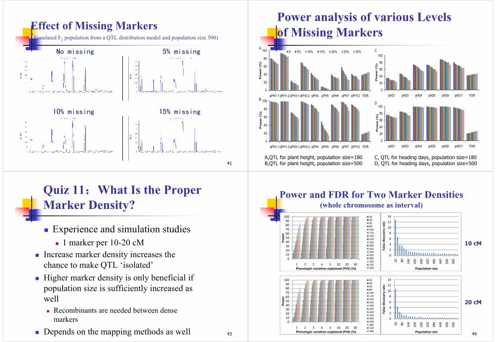
Effect of Missing Markers (Simulated F2 population from a QTL distribution model and population size 500)

41

No missing 5% missing

10% missing 15% missing

Power analysis of various Levels

of Missing MarkersA

B

C

0

20

40

60

80

100

qPH1-1qPH1-2qPH3-1qPH3-2 qPH4 qPH5 qPH6 qPH7 qPH12 FDR

Power (%)

0 5% 10% 15% 20% 25% 30%

0

20

40

60

80

100

qPH1-1qPH1-2qPH3-1qPH3-2 qPH4 qPH5 qPH6 qPH7 qPH12 FDR

Power (%)

C

D

0

20

40

60

80

100

qHD1 qHD3 qHD4 qHD5 qHD8 qHD11 FDR

Power (%)

0

20

40

60

80

100

qHD1 qHD3 qHD4 qHD5 qHD8 qHD11 FDR

Power (%)

A,QTL for plant height, population size=180B,QTL for plant height, population size=500

C, QTL for heading days, population size=180D, QTL for heading days, population size=500

Quiz 11：：：：What Is the Proper

Marker Density?

� Experience and simulation studies

� 1 marker per 10-20 cM

43

� Increase marker density increases the

chance to make QTL ‘isolated’

� Higher marker density is only beneficial if

population size is sufficiently increased as

well

� Recombinants are needed between dense

markers

� Depends on the mapping methods as well

Power and FDR for Two Marker Densities (whole chromosome as interval)

44

0

10

20

30

40

50

60

70

80

90

100

1 2 3 4 5 10 20 30

Po

we

r

Phenotypic variation explained (PVE) (%)

20

40

60

80

100

120

140

160

180

200

220

240

260

280

300

320

340

0

2

4

6

8

10

12

14

20

80

14

0

20

0

26

0

32

0

38

0

44

0

50

0

56

0

Fa

lse

dis

cov

ery

ra

te

Population size

0

10

20

30

40

50

60

70

80

90

100

1 2 3 4 5 10 20 30

Po

we

r

Phenotypic variation explained (PVE) (%)

20

40

60

80

100

120

140

160

180

200

220

240

260

280

300

320

340

0

2

4

6

8

10

12

14

20

80

14

0

20

0

26

0

32

0

38

0

44

0

50

0

56

0

Fa

lse

dis

cov

ery

ra

te

Population size

10 cM

20 cM

45

0

10

20

30

40

50

60

70

80

90

100

1 2 3 4 5 10 20 30

Po

we

r

Phenotypic variation explained (PVE) (%)

20

40

60

80

100

120

140

160

180

200

220

240

260

280

300

320

340

0

10

20

30

40

50

60

70

80

90

20

80

14

0

20

0

26

0

32

0

38

0

44

0

50

0

56

0

Fa

lse

dis

cov

ery

ra

te

Population size

0

10

20

30

40

50

60

70

80

90

100

1 2 3 4 5 10 20 30

Po

we

r

Phenotypic variation explained (PVE) (%)

20

40

60

80

100

120

140

160

180

200

220

240

260

280

300

320

340

0

10

20

30

40

50

60

70

80

90

20

80

14

0

20

0

26

0

32

0

38

0

44

0

50

0

56

0

Fa

lse

dis

cov

ery

ra

te

Population size

Power and FDR for Two Marker Densities(10cM interval, QTL in the middle)

10 cM

20 cM

Quiz 12：：：：What is QTL by E?

46

环境1 环境2

基因

型值

A. 互作模式1

基因型1

基因型2

环境1 环境2

基因型值

B. 互作模式2

基因型1

基因型2

环境1 环境2

基因型

值

C. 互作模式3

基因型1

基因型2

环境1 环境2

基因型

值

D. 互作模式4

基因型1

基因型2

47

Chromosome 1 2 3 3 5 5 7 7 7 8 8 8 9 10 12 12

Segment M4 M18 M21 M23 M35 M39 M49 M50 M51 M54 M56 M57 M59 M69 M77 M79

LODa E1 0.00 0.26 0.01 0.00 1.87 0.00 0.12 0.03 0.03 0.01 0.02 6.06 0.47 0.01 0.17 0.61

E2 0.00 1.05 2.88 4.66 0.95 0.14 0.35 0.30 0.11 0.13 5.84 3.92 2.89 0.22 0.12 0.05

E3 2.06 4.03 0.00 0.20 0.84 2.60 0.05 9.61 4.64 0.04 0.04 3.98 3.36 4.35 0.89 2.17

E4 0.04 0.04 0.00 4.03 0.05 0.32 0.04 0.02 0.49 0.70 0.05 15.89 6.26 2.57 0.10 0.24

E5 0.35 0.66 0.41 3.13 0.40 0.00 4.09 12.51 16.53 2.04 3.18 5.56 9.04 0.31 0.42 0.15

E6 0.13 0.38 1.06 1.35 0.30 0.22 0.32 0.02 0.18 0.00 0.16 1.84 4.15 0.90 0.29 0.05

E7 0.08 5.07 0.22 0.21 0.04 0.26 1.47 0.33 0.07 0.03 5.52 6.33 4.07 1.66 4.04 0.01

E8 0.01 0.00 0.02 0.45 2.16 1.54 0.01 0.02 0.01 0.67 0.17 16.89 10.01 0.01 0.00 0.00

ADDb E1 -0.11 -0.72 -0.12 -0.08 -2.13 0.06 -0.36 -0.19 0.25 -0.13 0.17 4.13 1.27 0.08 -0.35 -1.99

E2 -0.07 2.21 -2.98 4.35 -2.11 0.78 -0.88 -0.89 -0.72 0.54 4.43 4.51 4.62 -0.72 -0.43 -0.78

E3 3.89 4.69 0.11 -0.84 -2.03 -3.66 0.32 -6.12 5.11 -0.32 0.35 4.62 5.16 3.57 -1.21 5.68

E4 -0.24 -0.23 -0.04 2.05 -0.25 -0.61 -0.16 0.12 0.76 -0.67 -0.18 5.84 3.71 1.32 -0.20 -0.91

E5 1.06 1.22 -0.75 2.42 -0.94 0.07 2.30 -5.19 8.28 -1.59 2.20 3.86 6.40 0.60 -0.55 0.98

E6 -1.22 1.73 -2.29 2.88 -1.53 -1.30 -1.11 -0.30 -1.14 0.13 0.86 3.79 7.38 -1.87 -0.85 1.04

E7 -0.52 3.74 -0.56 0.61 -0.31 -0.78 -1.37 -0.69 -0.41 -0.19 3.11 4.29 4.01 1.44 -1.91 -0.21

E8 -0.09 0.05 -0.11 0.63 -1.63 -1.31 -0.09 -0.12 0.09 -0.62 -0.33 5.94 4.95 -0.09 0.03 0.09

PVEc E1 0.01 0.48 0.02 0.01 4.15 0.00 0.23 0.06 0.06 0.03 0.04 15.60 1.00 0.01 0.34 1.24

E2 0.00 2.24 6.60 11.44 2.04 0.28 0.69 0.59 0.24 0.26 14.54 9.36 6.66 0.46 0.25 0.10

E3 3.61 7.76 0.01 0.33 1.45 4.73 0.07 21.28 9.19 0.07 0.07 7.54 6.35 8.53 1.53 3.91

E4 0.04 0.05 0.00 5.62 0.06 0.38 0.05 0.03 0.59 0.86 0.05 34.66 9.49 3.35 0.11 0.29

E5 0.35 0.68 0.41 3.51 0.41 0.00 4.61 19.86 31.26 2.18 3.57 6.79 12.65 0.31 0.41 0.15

E6 0.46 1.37 3.88 4.99 1.07 0.78 1.07 0.07 0.60 0.02 0.55 6.60 16.93 3.06 0.98 0.17

E7 0.11 8.28 0.29 0.29 0.06 0.36 2.13 0.46 0.10 0.04 9.25 10.89 6.44 2.33 6.37 0.01

E8 0.01 0.00 0.02 0.52 2.66 1.70 0.02 0.02 0.01 0.73 0.17 35.08 16.53 0.01 0.00 0.00

Chromosome segments showing

QTL for ACEQuiz 13：：：：Does the Phenotypic Data Need to

Follow Normal Distribution?

48

F2h mg

2=0.90 , h p g

2=0 .10

B 1h mg

2=0.00

h pg2=1.00

B2h mg

2=0.95 , h p g

2=0 .05

F2 :3h m g

2=0.89 , h pg

2=0.11

R ILh m g

2=0 .88 , h pg

2=0 .12

F2h mg

2=0.80 , h p g

2=0 .10

B1h m g

2=0 .00

h p g2=0 .38

B2h mg

2=0 .87 , h p g

2=0 .05

F2 :3h m g

2=0 .82

h p g2=0 .12

R ILh m g

2=0 .84 , h pg

2=0 .13

F2h mg

2=0.70 , h p g

2=0 .10

B1h m g

2=0.00

h pg2=0 .23

B2h mg

2=0.78 , h pg

2=0.05

F2 :3h m g

2=0 .74

h p g2=0 .12

R ILh m g

2=0 .78 , h pg

2=0 .13

F2h mg

2=0.60 , h p g

2=0 .10

B1h m g

2=0 .00

h p g2=0 .17

B2h m g

2=0 .69 , h pg

2=0 .05

F2 :3h m g

2=0 .66

h p g2=0 .12

R ILh m g

2=0 .72 , h pg

2=0 .14

F2h mg

2=0.50 , h p g

2=0 .10

B1h m g

2=0 .00

h p g2=0 .13

B2h m g

2=0 .59 , h pg

2=0 .05

F2 :3h m g

2=0 .57

h p g2=0 .13

R ILh m g

2=0 .65 , h pg

2=0 .16

F2h mg

2=0.40 , h p g

2=0 .10

B1h mg

2=0.00

h pg2=0.11

B2h m g

2=0 .49 , h pg

2=0 .05

F2 :3h m g

2=0 .47

h p g2=0 .13

R ILh m g

2=0 .57 , h pg

2=0 .17

F2h mg

2=0.30 , h p g

2=0 .10

B1h mg

2=0.00

h pg2=0.09

B2h m g

2=0.38

h pg2=0 .06

F2 :3h m g

2=0 .37

h p g2=0 .14

R ILh m g

2=0 .47 , h pg

2=0 .19

F2h m g

2=0 .20

h p g2=0 .10

B1h mg

2=0.00

h pg2=0.08

B2h m g

2=0.26

h pg2=0 .06

F2 :3h m g

2=0 .26

h p g2=0 .15

R ILh m g

2=0 .34

h pg2=0.21

A single major gene and

many minor genes: the

distribution will be

normal.

However, the residual

needs to be normally

distributed.

There are methods that

can handle non-normal

distribution of residual.

A simulation: A QTL accounted for 80% of the phenotypic variation with additive effect 1.0

and located at 25 cM

49

0

10

20

30

40

50

8.5 9 9.5 10 10.5 11 11.5 12

Fre

qu

en

cy

Phenotypic value

-0.2

0

0.2

0.4

0.6

0.8

1

1.2

0 51

01

52

02

53

03

54

04

55

05

56

06

57

07

58

08

59

09

51

00

10

51

10

11

51

20

12

51

30

13

51

40

14

51

50

15

51

60

Est

ima

ted

eff

ect

1D-scanning on one chromosome, step=1cM

ICIM

IM

0

20

40

60

80

100

0 51

01

52

02

53

03

54

04

55

05

56

06

57

07

58

08

59

09

51

00

10

51

10

11

51

20

12

51

30

13

51

40

14

51

50

15

51

60

LO

D s

co

re

1D-scanning on one chromosome, step=1cM

ICIM

IM

Quiz 14：：：：Do Mapping Component Traits Help?

50

Effect Trait I Trait II Addition Subtraction Multiplication Division

Mean 25 20 45 5 500 1.2563

A1 1 0 1 1 20 0.0503

A2 1 0 1 1 20 0.0503

A3 0 1 1 -1 25 -0.0631

A4 0 1 1 -1 25 -0.0631

A12 0 0 0 0 0 0

A13 0 0 0 0 1 -0.0025

A14 0 0 0 0 1 -0.0025

A23 0 0 0 0 1 -0.0025

A24 0 0 0 0 1 -0.0025

A34 0 0 0 0 0 0.0063

A123 0 0 0 0 0 0

A124 0 0 0 0 0 0

A134 0 0 0 0 0 0.0003

A234 0 0 0 0 0 0.0003

A1234 0 0 0 0 0 0

Using Composite Trait Reduces

Detection Power and Increase FDR

51

QTL Trait I Trait II Addition Subtraction Multiplication Division

Model I Power (%) Q1 95.10 69.60 69.30 55.20 50.50

Q2 94.80 69.80 70.40 54.10 50.90

Q3 92.50 67.20 65.30 76.90 75.20

Q4 94.50 68.40 65.40 77.80 75.20

FDR (%) 21.63 22.98 27.42 28.05 28.07 29.68

Model II Power (%) Q1 95.40 67.40 65.60 54.80 49.90

Q2 92.90 62.40 66.00 50.00 49.90

Q3 93.70 69.90 67.00 79.20 74.90

Q4 91.90 62.40 64.90 73.50 72.90

FDR (%) 21.35 22.18 28.76 28.59 28.07 28.89

Model III Power (%) Q1 95.20 66.60 52.40 53.60 37.70

Q2 95.00 69.20 51.60 54.70 36.40

Q3 92.90 63.40 47.80 69.70 56.20

Q4 92.60 61.50 49.90 72.60 58.00

FDR (%) 19.78 23.44 28.83 27.71 29.74 30.18

Quiz 15: Is Selective Genotyping

(SG) Useful?

52L

LL

H

HH

LH

N

pp

N

pp

ppt

2

)1(

2

)1( −+

−

−=

Low tail

High tail

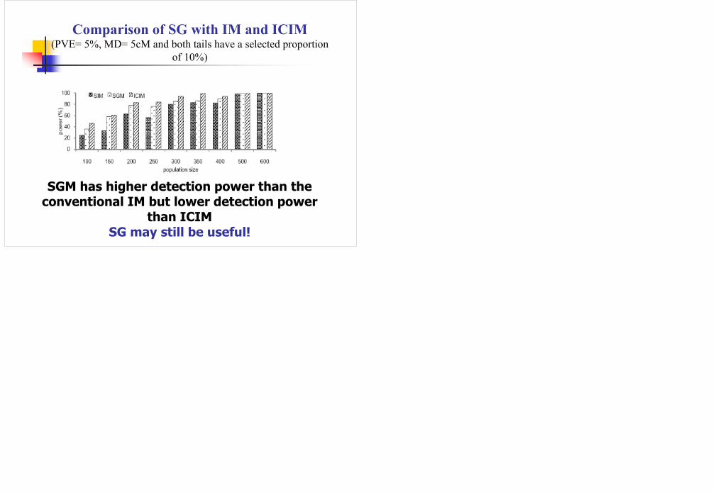
Comparison of SG with IM and ICIM(PVE= 5%, MD= 5cM and both tails have a selected proportion

of 10%)

SGM has higher detection power than the conventional IM but lower detection power

than ICIMSG may still be useful!