tutorial: collection efficiency calculation and running...

Tutorial: Collection efficiency calculation and running wet and run-

back analysis on wing

Introduction

The first step in every aircraft icing analysis is to calculate the droplet collection/impingement characteristics of the aircraft body under a given flight condition. The parameter of interest in the analysis is the collection, or catch efficiency. This surface quantity represents the ratio of the mass-flux of the impinging droplets to the mass-flux in the free stream. Only after performing the collection calculations, subsequent anti-icing or ice build-up calculations can be undertaken.

When anti-icing system is on and supercooled droplets hit the aircraft body they form a water film on the surface. This film runs over the surface and can separate at edges and strip under high shear and release as water droplet particles again. This is called as running wet and run back scenario.

Eulerian Wall Film (EWF) model can be used to predict collection efficiency and simulate running wet and run back kind of problems. EWF model can be coupled with:

• Discrete Phase Model – Particles are collected on the wall to form the film

• Eulerian Multiphase Model – Secondary Phase mass is collected on the wall to form the film

In EWF model, the film is not resolved using mesh normal to the surface, instead this model uses a virtual film on the surface. In many cases we would be interested in modeling a thin film flow which can separate, strip and evaporate but does not affect the core flow-field. This kind of thin film modeling is computationally expensive in general multiphase frame work where we will need very fine mesh to model the film and also need to calculate inter-phase flux accurately. EWF model can only be used with 3d solver and EWF model assumes that film always flows parallel to the surface so normal component of film velocity is zero. The film is assumed to have a parabolic velocity profile & bilinear temperature profile across its depth.

Problem Description

The goal of this tutorial is to model running film on a NACA-0012 airfoil and determine the collection efficiency. The Airfoil is at 5 degrees angle of attack, Mach 0.4 with a Liquid Water Content (LWC) of 1g/m^3 in freestream. In ANSYS FLUENT 14 this film accretion modeling functionality with Eulerian multiphase is available via a User Defined Function (UDF) code. It is planned to incorporate this functionality natively in a future release.



2

In this tutorial you will learn:

• How to couple EWF model with Eulerian multiphase approach to create film.

• Use of EWF model to determine collection efficiency. • How to model particle stripping.

• How to see particles separated or stripped from film.

Prerequisites

This tutorial is written with the assumption that you have completed Tutorial 1 from the ANSYS FLUENT 14.0 Tutorial Guide and that you are familiar with the ANSYS FLUENT navigation panels and the menu structure. Therefore, some steps in the setup and solution procedure will not be shown explicitly.

Preparation

1. Copy the files, (NACA_0012.msh, film_accretion.c) to the working folder.

2. Use FLUENT 14 Launcher to start the 3DDP version of ANSYS FLUENT.

Setup and Solution Stage1: Solution of Multiphase flow

In this section, we will be discussing the setup and solution of flow of air & water droplets mixture over the wing surface. We will use Eulerian multiphase approach to model this flow. Step 1: Mesh

1. Read the mesh file (NACA_0012.msh)

File �� Read �� Mesh

2. Change the view

Display �� Views �� Front

3. Display Mesh on symmetry plane

Display �� Mesh �� sym_1

a. Zoom in as shown in below figure.

b. Give name as view1 and click save.



3

Fig 1: Mesh distribution in sym_1

Step 2: General Settings General

1. Check the mesh

a) General � Check

ANSYS FLUENT performs various checks on the mesh and reports the progress in the console. Pay attention to the minimum volume reported and make sure this is a positive number. Note: Warning for high aspect ratio cells is because of very fine mesh near the wing surface to resolve the boundary layer. This warning can be ignored.

Step 3: Models

Models.

1. Setup Multiphase Model

Models � Multiphase � Edit

a) Select Eulerian under model.

b) Click OK to close the Multiphase Model.

2. Enable the Energy Equation.

Models � Energy � Edit

a) Click ok to close the Energy panel

Click ok in the information dialogue box.



4

3. Select the Standard k-epsilon turbulence model.

Models � Viscous � Edit

a) Select k-epsilon (2 eqn).

b) Ensure that Standard under k-epsilon Model.

c) Ensure Standard Wall Functions under Near Wall Treatment.

Step 4: Materials

Materials

1. Change the material properties

Materials � Air � Create/Edit

a) Change density to ideal gas.

b) Click Change/Create.

2. Add water-liquid

a) Click Fluent Database... to open the Fluent Database Materials panel.

b) Select water-liquid (h2o<l>) from the Fluent Fluid Material list.

c) Click Copy and close the Fluent Database Materials and Materials panel.

d) Change the Name to water-liquid-eulerian.

Note: This will allow choosing same water-liquid material for DPM Phase in

later stage.

e) Change Chemical Formula to h2o<l>-e.

f) Click Change/Create.

g) Click Yes to overwrite.

h) Close the Material Panel.

Step 5: Phases

Phases

1. Set Phase-1-Primary Phase

Phases � Phase -1 – Primary Phase � Edit

a) Change the name to air.

b) Select Phase Material as air.

c) Click OK to close the Primary Phase dialogue box.



5

2. Set Phase-2-Secondary Phase

Phases � Phase -2 – Secondary Phase � Edit

a) Change the name to water-liquid-eulerian.

b) Select Phase Material as water-liquid-eulerian.

c) Change the diameter to 1.6e-05

d) Click OK to close the Secondary Phase dialogue box.

Step 6: Boundary Conditions

Boundary Conditions

1. Set the boundary conditions for mixture phase at far-field_1 zone.

Boundary Conditions � far-field_1

a) Ensure that Pressure inlet is selected.

b) Select Mixture under Phase.

c) Click edit and set the following values.

Parameters Values Gauge Total Pressure (Pa) 11809.64 Supersonic/Initial Gauge Pressure (Pa) 0 Direction Specification Method Direction Vector Turbulence: Specification Method Intensity and Viscosity Ratio Turbulence Intensity (%) 1 Turbulent Viscosity Ratio 5

d) Click OK to close the Pressure inlet panel.

2. Set the boundary conditions for air phase at far-field_1 zone.


a) Select air under Phase.

b) Click edit.

Parameters Values X- Component of Flow Direction 0.9961947 Y- Component of Flow Direction 0.0871557 Z- Component of Flow Direction 0 Total Temperature (K) 309.6

Note: You have to go to Thermal tab to set Total Temperature



6

3. Set the boundary conditions for water-liquid-eulerian phase at far-field_1 zone.


c) Select water-liquid-eulerian under Phase.

d) Click edit.

Parameters Values X- Component of Flow Direction 0.9961947 Y- Component of Flow Direction 0.0871557 Z- Component of Flow Direction 0 Total Temperature (K) 309.6 Volume Fraction 1e-06

Note: You have to go to Multiphase tab to set Volume Fraction.

4. Set the boundary conditions for mixture phase at far-field_2 zone.


a) Ensure that Pressure inlet is selected.

e) Select Mixture under Phase.

f) Click edit and set the following values.

Parameters Values Gauge Pressure (Pa) 0 Turbulence: Specification Method Intensity and Viscosity Ratio Turbulence Intensity (%) 1 Turbulent Viscosity Ratio 5

g) Click OK to close the Pressure inlet panel.

5. Set the boundary conditions for air phase at far-field_2 zone.


e) Select air under Phase.

f) Click edit.

g) Set Backflow Total Temperature to 300 K.

h) Click OK to close the panel.

6. Set the boundary conditions for water-liquid-eulerian phase at far-field_2 zone.


i) Select water-liquid-eulerian under Phase.

j) Click edit.



7

k) Set Backflow Total Temperature to 300 K.

l) Set Backflow Volume Fraction to Zero.

7. Check Boundary Conditions for other zones.

a) Ensure that symmetry is selected for sym_1 and sym_2.

b) Ensure that wall is selected for wing_lower and wing_upper.

Step 7: Solution Methods

Solution Methods

1. Set Solution Methods

a) Set the following under solution methods.

Pressure-Velocity Coupling Scheme

Phase Coupled SIMPLE

Gradient Green-Gauss Node Based

b) Keep discretization schemes for other equations to default.

Step 8: Monitors

Monitors

1. Set criteria for convergence.

Monitors � Residuals � Edit

a) Set Convergence criteria to none.

b) Ensure that plot is enabled.

c) Click OK to close the dialogue box.

Step 9: Solution Initialization

Solution Initialization

1. Initialize the Solution

a) Select Standard initialization under Initialization methods.

b) Select far-field_1 under Compute from.

c) Click Initialize to initialize the solution.



8

Step 10: Save the case file

File � Write � Case

a) Type the file name as airfoil_step1.cas.gz

Step 11: Run Calculation

Run Calculation

1. Set Run calculation parameters

a) Enter 200 for number of iterations.

b) Click Calculate.

Step 12: Save the case and data files

File � Write � Case/data


Step 13: Post Processing

a. Display residual



9

b. Display Velocity magnitude for air in sym_1 Note: Make sure that view1 is selected in Display.

Display � Mesh

a) Choose Faces under option.

b) Select wing-lower & wing-upper under Surfaces & click Display.

c) Zoom in and rotate wing surfaces to get view as shown in below figure.

d) Close the Panel.



10

Display � View

a) Give name as view2 and click save.

b) Click Write, Write Views panel will open.

c) Select view2 and click OK.

d) Type file name as view2 and click OK.

c. Contour of Volume fraction of Water-Liquid-eulerian on wing_lower and wing_upper surface.

Volume fraction contour shows where water particles are collected. Now in the next stage we will discuss about modeling of film using Stage 1 solution.



11

Stage 2. Film Accretion

In this section, film accretion is modeled through a UDF. Secondary phase flux normal to the wall boundary removed at the walls where the film is modeled & liquid film is formed from the removed secondary phase.

Step 1: Compile & Read UDF

Go to Define� User Defined� Functions�Compiled and change the Library name to lib_accretion. Compile the UDF file “film_accretion.c” and then click “Load”.

While the compiled library is being read in, the list of all the UDFs in that library will be

printed on the Fluent console, as shown in the above image. In the subsequent sections, these UDFs will be ‘hooked’ to the appropriate fields.

Step 2: Cell Zone Conditions

Cell Zone Conditions

1. Set water-liquid-eulerian Phase

a) Select Water-liquid-eulerian under Phase.

b) Click Edit.

c) Enable Source Terms.

d) Click Edit next to Mass.

e) Set Number of mass sources to 1.

f) Select euler_capture_mass_src.

g) Click OK.

h) Follow the same procedure to set momentum and energy sources

X-Momentum euler_capture_x_mom_src

Y-Momentum euler_capture_y_mom_src

Z-Momentum euler_capture_z_mom_src

Energy euler_capture_heat_src



12

Step 3: Models

Models

1. Switch ON Eulerian Wall Film Model

Models � Eulerian Wall Film � Edit

a) Enable Eulerian Wall Film Model.

b) Enable Solve Momentum.

c) Select water-liquid-eulerian under Film Material.

Note: Film material should be always same as secondary phase material.

d) Go to Solution Method and Control Tab

e) Set the Maximum Thickess as 0.01m.

Note: Choose Maximum Thickness such that during solution, the film thickness never hits this

maximum limit. If the film thickness value hits this limit then the solution will not be

appropriate.

f) Set the Time Step Size to 0.0001s.

g) Click OK to close the panel.

Fig 2: Panel of Eulerian Wall Film Model



13

Step 4: Boundary Conditions

Boundary Conditionsl

1. Enabling Film Modeling on the boundaries

a) Select wing_lower.

b) Select Mixture under Phase.

c) Click Edit.

d) Go to Wall Film Tab.

e) Enable Eulerian Wall Film.

f) Enable Initial Condition.

g) Make sure that all the parameters are set to Zero.

h) Click OK to close the panel.

Fig 3: Panel of Eulerian Wall Film Boundary Condition

i) Follow the same procedure to set Boundary Condition for wing_upper



14

Step 5: Initialize the Wall Film Model.

Models � Eulerian Wall Film � Edit

a) Go to Model Options and Setup tab.

b) Click Initialize.

c) Click OK to close the panel.

Step 6: Enable Film Accretion

a) Go to TUI.

b) Type (enable-film-accretion #t).

c) Press Enter.

Step 7: Save the case.

File � Write � Case



Run Calculation


e) Enter 200 for number of iterations.

f) Click Calculate.

Step 9: Save the case and data file

File � Write � Case/data




15

Step 10: Post-Processing a) Residual plot

Note: For film solution there is no residual plot. But, the film solution can be monitored from

console by monitoring max_cfl.

• Choose the film timestep such that “max_cfl” does not go to very high value.

• “max_cfl” value less than 0.01 is reasonable, but for some cases it can go up to 0.5.



16

b) Contour of Eulerian Wall Film �� Film Thickness on wing_lower and wing_upper. Display � View

a) Click on Read and read the view2.vw file

c) Contour of Eulerian Wall Film �� Film Velocity Magnitude on wing_lower and

wing_upper.



17

Stage 3. Collection Efficiency calculation

In stage 2 we obtained the film solution using EWF model. In this section, we will discuss how to use EWF model to calculate the collection efficiency.

Collection Efficiency is defined as:

Impingement Mass Flux/(LWC * Free stream Velocity)

Impingement mass flux is calculated from the solution. So we need to set two film

parameters to obtain the collection efficiency:

i. ‘secondary-phase-vel � this is the far field flow velocity (m/s) ii. ‘secondary-phase-conc � this is the far field liquid water content (LWC)

(kg/m^3) iii. (get-film-parameter ‘secondary-phase-vel) � to display the current value & (set-

film-parameter ‘secondary-phase-vel 138.77) � to set the variable value a) For this case Free stream velocity is 138.8 m/s & LWC is 0.001 kg/m^3 b) Go to TUI and type

i. (set-film-parameter ‘secondary-phase-vel 138.8) ii. (set-film-parameter ‘secondary-phase-conc 0.001)

iii. it 1.

Note: Atleast 1 iteration is required to do collection efficiency calculation.



18

c) Plot “Eulerian Wall Film � Film Secondary Phase Collection Coef on wing_lower and wing_upper.

Fig: Film Secondary Phase Collection Coeff

Step 1: Create line at the middle of wing for post-processing

Surface �� Iso-Surface

a) Select Mesh under Surface of Constant. b) Select Z-Coordinate. c) Select Mixture under Phase. d) Under Iso-values set 0.5. e) Select wing_lower and wing_upper under From Surface. f) Enter name as mid-line. g) Click Create.

Step 2: Plot Film Secondary Phase Collection Coef

Plots � XY Plots

a) Select Eulerian Wall Film under Y Axis Function. b) Select Film Secondary Phase Collection Coef. c) Choose mid-line under Surfaces. d) Click Plot. e) Close the panel.



19

Fig: XY Plot of Film Secondary Phase Collection Coef

Stage 4. Viewing Stripped/Separated DPM Particles from the film

During run back process, the film can strip off due to high shear and/or separate at edges and re-release particles. In this section, we will discuss how to see stripped or separated particles.

Step 17: Define Dummy Injection.

Define � Injections � Create.

1. Choose Injection Type to Single.

2. Choose Material as a water-liquid.

3. Set X, Y, Z positions as

X- Positions (m) 10

Y- Positions (m) 10

Z- Positions (m) 0.5

Note: Make sure that injection is well inside the domain.

4. Click OK to close the panel.

5. Close the Injection Panel.



20

Materials

3. Change the material properties

Materials � Inert Particle � water-liquid � Create/Edit

a. Change the Name to water-liquid-eulerian-particle.

Note: Secondary phase and dpm particle material properties should be same and

secondary phase material name should be part of dpm particle’s material name (“water-

liquid-eulerian” is a common part between two names).

b. Change Chemical Formula to h2o<l>-e-p.

c. Click Change/Create.

Step 18: Enable DPM Collection and Particle Stripping Option.

Models � Eulerian Wall Film Model � Edit

a) Enable DPM Collection

b) Enable Particle Stripping.

c) Set Critical Shear to 140 n/m2.

Note: Unit of Critical Shear is hard coded and it is always in n/m2 which means independent

of pressure unit.


Run Calculation


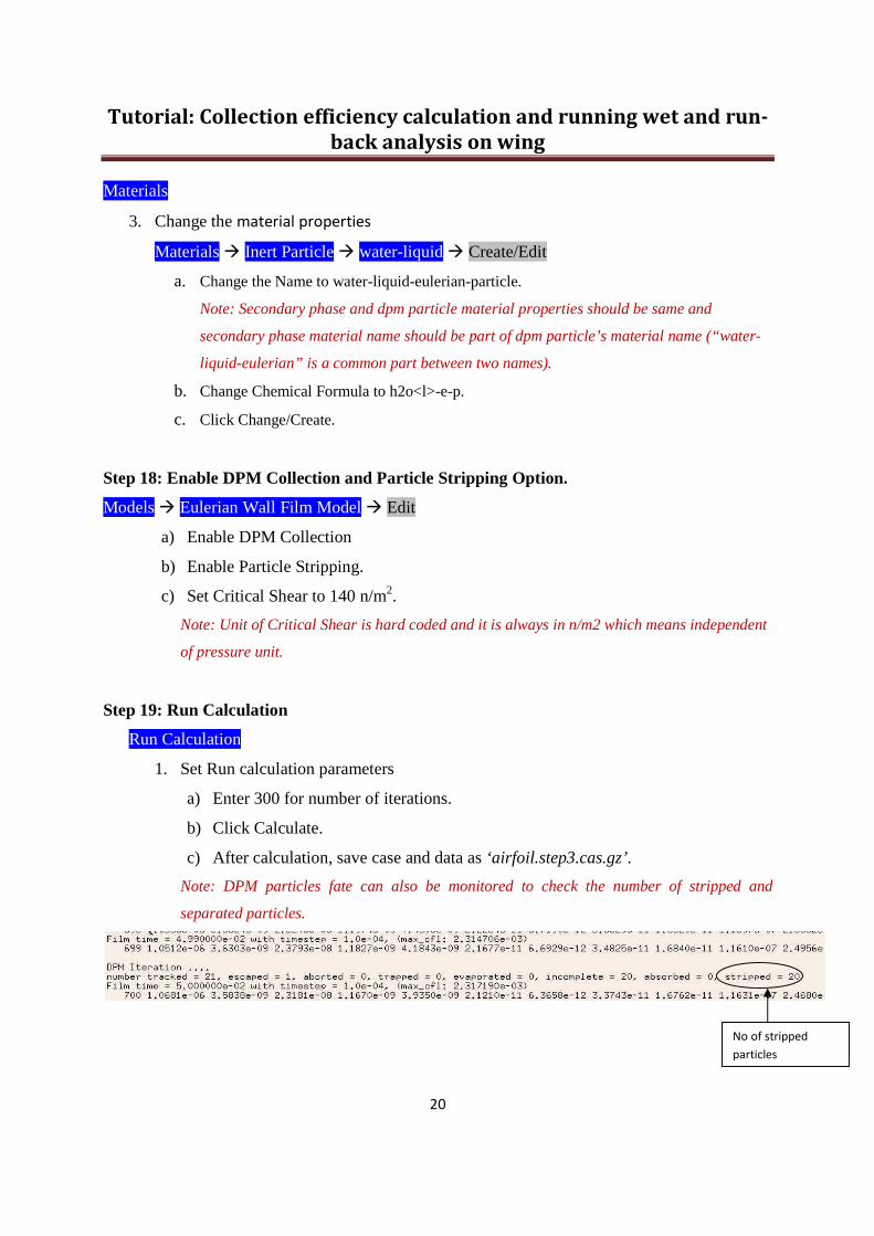
a) Enter 300 for number of iterations.

b) Click Calculate.

c) After calculation, save case and data as ‘airfoil.step3.cas.gz’.

Note: DPM particles fate can also be monitored to check the number of stripped and

separated particles.

No of stripped

particles



21

Step 20: Post-Processing

a. Residual plot

b. Contour of Wall Shear Stress on wing



22

c. Particle Track- Stripped particles

Graphics and Animations � Particle Tracks

i. Enable Draw mesh. (Mesh Display panel will be opened)

ii. Enable Faces.

iii. Select wing-lower & wing-upper.

iv. Close the Mesh Display panel.

v. Select injection-0 under Release from Injections.

vi. Click Display.

Note: Particle are stripped off from high shear region

Tutorial: Collection efficiency calculation and running wet and run

Best Practices & Important Notes

• It is always good to first Eulerian wall film.

• It is always good to start with smaller film timesize to keep max_cfl under reasonable limit.

• Note that “Film Secondary Phasewill need to do at least 1 iteration for the variable to have any value after you reload case and data file in a new Fluent session.

• In ANSYS FLUENT 14stripping model but critical Weber number based stripping criteria is also available through a scheme command.

o To access that, Fluent console.

o Once you enable this feature"Critical Weber Number" instead but the GUI doesn't change.

o Critical Weber number criterion is depends upon film thickness, surface tension and velocity of flow. It is planned to make this as a default criterion for stripping.

o Shear based Weber number is defined as:

Collection efficiency calculation and running wet and run


23

Best Practices & Important Notes:

first achieve a converged multiphase flow solution and then solve for

lways good to start with smaller film time-step size and then increase to keep max_cfl under reasonable limit.

Note that “Film Secondary Phase Collection Coef” is not saved in will need to do at least 1 iteration for the variable to have any value after you reload case

new Fluent session. ANSYS FLUENT 14, we have critical shear stress based stripping criterion for

stripping model but critical Weber number based stripping criteria is also available scheme command.

you need to type (enable-film-weber-strippingFluent console. Once you enable this feature, the number you specify as "Critical Shear" becomes "Critical Weber Number" instead but the GUI doesn't change.Critical Weber number criterion is better that critical shear stress depends upon film thickness, surface tension and velocity of flow. It is planned to make this as a default criterion for stripping. Shear based Weber number is defined as:

Where,

Vs = Shear Velocity

Hf = Film Thickness

ρf = Film Material Density

σ = Surface Tension

µf = Film Viscosity

Collection efficiency calculation and running wet and run-

flow solution and then solve for

and then increase the time-step

Coef” is not saved in the data file. So you will need to do at least 1 iteration for the variable to have any value after you reload case

we have critical shear stress based stripping criterion for stripping model but critical Weber number based stripping criteria is also available

stripping-criterion #t) in

the number you specify as "Critical Shear" becomes "Critical Weber Number" instead but the GUI doesn't change.

better that critical shear stress criterion as it depends upon film thickness, surface tension and velocity of flow. It is planned to



24

Appendix: Collection Efficiency

The collection efficiency (β) is calculated as the ratio of the amount or mass of water collected on the surface to the total mass of droplets being injected at the inlet. Both

Langragian (or DPM) & Eulerian methods can be used to determine the collection efficiency.

Eulerian approach:

• Solves for Transport equations for the droplet phase � Mass, momentum, and volume fraction

• Easy to specify droplet freestream condition and smooth impingement region can be achieved.

• But in the Eulerian approach each droplet size required to solve as a separated phase with one set of transport equation so it becomes very memory intensive.

Discrete Particle Method (DPM) approach:

• Water droplets modeled as discrete packets of particle:

• Very easy to specify droplet size distribution at freestream.

• The main difficulty of the Lagrangian approach lies in tracking every droplet history and in establishing appropriate boundary conditions for the droplet concentration in two and three-dimensional flows.

• A large number of droplets need to be considered to achieve an accurate representation of the dynamics & to obtain a “smooth” impingement which becomes computationally expensive.

∞

=V

nv ˆ.r

αβ

m

Raccretion

&=β

tutorial: collection efficiency calculation and running...

Documents