Erik Dahlén

Lund ObservatoryLund University

Turbulent concentrationof particles

Degree project of 15 higher education creditsMay 2012

Lund ObservatoryBox 43SE-221 00 LundSweden

2012-EXA64

1 Svensk sammanfattning (for English turn page)

Den bakomliggande teorin om planetbildning är att planeterna bildas sam-tidigt som stjärnan och därför av samma material som stjärnan. Därför måstedessa stoft- och gaspartiklar bindas samman till planeter. Teorin säger attdetta görs i en disk runt stjärnan vilken uppstår vid stjärnbildning för attbevara rörelsemängdsmomentet och sådana diskar har observerats och skulleförklara varför alla planeter i vårt solsystem roterar i samma plan. Man kandela in denna process i tre faser där olika krafter dominerar. Den första ärnär de enskilda particlarna binds samman av elektriska krafter till mikrome-ter stora partiklar. Den andra är när dessa mikrometer stora partiklar bindssamman till kilometer stora objekt (planetesimal på engelska). Den tredjeoch sista är när dessa kilometer stora objekt binds samman av gravitationtill tusen kilometer stora kroppar som sedan är så stora att de uppfyller def-initionen som planet. Under denna process är det steg två som inte riktigtkan förklaras, eftersom både gravitationskraften och de elektriska krafternaär försumbara. En teori för att lösa detta är att turbulens i disken runt stjär-nan skulle kunna ansamla så många partiklar på ett ställe att gravitationenskulle ta över och bilda objekt på över en kilometer i diameter.

Turbulens är en makroskopisk rörelse i en gas, eller vätska, som är kaotisk.Vid turbulens uppstår det virvlar som i den fria rymden har ett lågtryck imitten av sig. Detta uppstår då gasen i virvlen känner en centrifugalkraftutåt så måste detta kompenserar av en tryckkraft inåt som enbart kan uppståom virveln har ett lägre tryck i mittan än utanför. Om man skulle ha par-tiklar i en sådan turbulent gas kommer de att �yga ut ur virvlarna eftersomde också kommer känna centrifugalkraften men inte tryckkraften som gasenkänner. Hur e�ektivt de lämnar virveln beror på hur väl de känner av gasensrörelse, vilket beror på hur väl sammankopplade de är.

Jag har därför försökt simulera en turbulent gas med partiklar enligtovan beskrivning. Det har gjorts genom att använda Pencil Code för attnumeriskt beräkna vad som händer med en gas och dess partiklar över tidennär man inför turbulens. Detta har gjorts genom att anta att gasen följerNavier-Stokes ekvation och att partiklarna är kopplade till gasen med enfriktionstid. Dessa simuleringar visar att man med rätt friktionstid, vilkenavgör hur väl gasen och partiklarna är kopplade, kan man få en myckethög ökning av partikelkonsentrationen på vissa ställen. Simuleringarna visaräven att upplösningen och gasens viskösitet inte har någon större betydelseför partikelansamlingarna.

3

2 Abstract

Turbulence which can increase the maximum particle density in some regionis interesting for planet formation since the process for building up planetshas some problem. Planets are formed by dust grains sticking together intoplanets during the star formation period and the major problem is the thegrowth from cm to km scale. During this phase both the microscopic molec-ular forces and the macroscopic gravity are negligible, therefore are thereno well accepted theory for the entire planet formation phase. One idea isthat turbulence could help in clustering particles together so that self gravitytakes over and planetesimal can form.

The Pencil Code has been used to simulate how turbulence a�ects theparticle density distribution for dust particles in a gas. In a 2D simulationone can �nd a peak of the particle density at some values of the frictiontime, the highest peak had 84 times higher maximum particle density thanthe mean particle density when averaged from time 0 to 4900. This indicatethat turbulence could contribute to planetesimal formation. The simulationalso shows that 2D has a inwards cascade that follows the E(k) ∝ k−3 line.The turbulence was arti�cially introduced with so called forced turbulence,which is when one add turbulence without thinking of its physical origin. Ifone stops the forced turbulence after a while one can see how the eddies inthe turbulence dissipates and how the smallest eddies dissipates �rst sincethe viscosity a�ects them more.

4

3 Planet formation

The main idea is that planets are formed during the star formation period,which means that the planets are formed by the same gas cloud as the star(often called the protostar phase). The theory is that at a late stage ofthe star forming process the star will be surrounded with a disk, a so calledprotoplanetary disk. Such disks have been observed by spectroscopy of OrionHH 3 which showed that previous detected structure were protoplanetarydisks (O'dell, 1993). This would explain why the planets in our solar systemare all orbiting in the same plane. For this model to work individual dustgrains must be able to stick together into planets. To make any sense ofthis we divide this process into three regimes where di�erent forces dominateeach phase which gives rise to di�erent properties.

The �rst part we call the dust phase. In this phase the particles are µmin size. In this range the molecular forces dominate so that the particles cangrow by sticking if they collide due to induced dielectric forces such as vander Walls (Dominik, 2006).

The second part is the rock phase, which is when the body is from 10cmto some hundred meters in diameter. In this regime neither gravity normolecular forces are strong enough to make them grow and most collisionwill not end up in building any bigger bodies.

Planetesimals are the third and last phase before planets are formed,which is from km scale and 1000km. In this phase gravity starts dominatingand will be the force that brings bodies together in collisions. It is easy tosee that this is a runaway situation where every collision will make it growand the bigger the planetesimal is the stronger will the gravitational force be,therefore all growth beyond this size will also be gravitationally dominated.

The rock phase is the part with most problems in the theory. One ofthe problems is the radial drift time scale which is in the order of somehundred years (Philip, 2010). Radial drift, which is when particle in theprotoplanetary disk drifts inward to the star, occur since the rocks are notwell coupled to the gas and therefore do not move with the gas but with ahigher speed (the gas is slowed down due to a pressure gradient force whichthe particle do not fell as strong as the gas). This higher speed makes therock feel a headwind (when the rock hits new gas all the time because of itshigher speed) which transfers some of the rocks angular momentum to thegas and hence the rock spiral inward to the star. This implies that it willonly take a rock of this size some hundred of years to drift from the disk into

5

the star, hence rocks has only a few hundred of years to form planetesimal.There is more then one theory which explain how the rock phase can pass

in the speed which it needs. Many of these theories are still debated and areunder research. I have looked into the idea that eddies in turbulence couldgather particles to high enough density for planetesimal formation to startin one place of the disk while some other parts gets low particle density. Themain concept is that the particles feel a drag force from the gas when the gasswirls around which makes the particles moves out from the major eddies.

4 Turbulence

Turbulence is interesting, for a number of reason such as �ow in tubes andmixing an inhomogeneous �uid into a homogenous �uid. Mixing can not beneglected when it is several orders of magnitude more e�cient than randommovements (Manneville, 2004). In this thesis the main interest lays in thecreation of eddies and behavior of eddies, explained further down.

Fluids have typically three motions: the micro scale movement, lami-nar �ows and turbulent �ows. Micro scale movement is always consideredbeing chaotic. Laminar �ows occur when the �uid is moving in one direc-tion smooth and at a constant rate. Turbulent �ows are somewhere betweenchatic and laminar. Like laminar �ows turbulent �ows are also macroscopicin nature and move part of the �uid from one place to another, but like microscale movement turbulent �ows are characterized by chaotic movement andinhomogeneous velocity (both in direction and speed). Turbulent �ows, likelaminar �ows, are created by a macroscopic force, e.g. by pressure gradientin a gas which can create a laminar �ow when the gas moves into equilibriumor gravity pulling water downstream towards a stone which may cause tur-bulence in the water just after the stone (Frisch, 1995). When the force is nolonger "active", which means that the force no longer adds any energy to the�uid, the turbulence will start decaying and eventually turns kinetic energyinto thermal energy. Before the decay, the turbulence can have a period ofdevelopment, which means that eddies could continue to build up like it doesduring the active phase (Manneville, 2004).

One way to measure whether a �ow should be turbulent or not is bycalculate the Reynolds number which is de�ned as

Re = lu/ν (1)

6

(Cuzzi, 2001), where l is the length scale of the system (the same as thediameter of the largest eddy), u the speed of the eddies compare to thebackground gas (often the same as the rotation speed of the largest eddy) andν is the molecular viscosity. A larger Reynolds number implies an increasedstrength of the turbulence.

An eddy is a rotation, or swirling, in a �uid during turbulence. Eddiesoften occur after a �uid has hit an object, but they can occur everywherein a turbulent �ow. Eddies can both decay to smaller ones, as in �gure1, and build up to bigger ones. To decay into smaller ones can happen toall eddies and the characteristic decay time is given by l/u (Burden, 2008),also known as eddy turn over time, where l is the length scale and u thevelocity scale. This process continues until the eddies become so small thatthe viscosity term in the Reynolds number starts dominate. To merge severalsmaller eddies into one bigger requires that the smaller ones are rotating inthe same plane, hence turbulence in 3D are unlikely to merge into biggereddies. Turbulence in 2D are likely to merge into bigger eddies, due to alleddies are in the same plane. Inside an eddy in free space will there alwaysbe a low-pressure, this because all rotation creates a centrifugal force andthe only way to balance this out is by a pressure gradient which implies thatthere must be a higher pressure outside the eddy. In some system like onearth are there eddies with high pressure in the center of the eddy. In theatmosphere eddies are created by air going down from high altitude to low,or the other way around, and the rotation is created by the Coriolis force sothe rotation change on the di�erent side of the equator (eddies circle highpressure clockwise and low pressure anticlockwise on the northern hemisphereand vice versa) (Wallace, 2006).

7

Figure 1: This illustrate that an eddy is a rotation of the gas, that an eddyin free space will always have a low pressure inside of it and the conceptthat eddies could cascade both inverse, the bottom arrow, and direct, thetop arrow.

If we let l0 be the length scale of the largest eddy, we can make a listof all the smaller length scales as l0/2, l0/4, ...l0/n. We can then sum up allthe energy for every eddy with the same length scale, and then plot themas a function of their wave number (which is related to the length scale ask ∼ 1/l). This plot would look somewhat like �gure 2. The energy containingrange is where the largest eddies are present, this is limited because of themacroscopic property of the system that does not let the eddies grow bigger.Dissipation range is where the energy decreases because of the molecularviscosity is turning the turbulent energy into thermal energy. The dissipationrange could have a spike in this plot which indicates that one of the smallesteddies have a lot of energy just before decaying. Between those two we havethe inertial range, where the molecular viscosity of the �uid is negligible butthe range of eddies is not bound by the size of the system. The inertial rangeis, if one plots the axis logarithmic, a constant slope which often has one ofthe two values −3 or −5/3 (Kraichnan, 1966).

8

Figure 2: This is the shape of the spectrum of isotropic and homogeneousturbulence. It is an illustration like �g 7.4 in Instabilities, chaos and tur-bulence by Manneville. The x-axis is the wavenumber and the y-axis is theenergy at that wavenumber, both axes are logarithmic.

The friction time τ of the particles is a constant, with dimension time, thattells how much the gas interacts with the particles. The following equationgives us the acceleration the particles gets from the gas.

dv

dt=

1

τ(u− v) (2)

where v is the speed of the particle and u is the speed of the gas (Markiewicz,1991). The friction time is dependent on the properties of the particle, andthen mainly its size, due to di�erent size are coupled to the gas di�erent well.

The following equation is called the continuity equation and is used insimulation with �uids.

dρ

dt+5ρu = 0 (3)

9

(Elaine, 1987), where ρ is the density and u the velocity �ow which is howmuch mass �ows from one region to another at one time. This equation makessure that the mass is conserved in the simulation. Simply this equation onlyallows the density to change in one region by the amount of mass passinginto it and/or out from it to the adjacent regions.

Under the assumption that the gas is incompressible and the viscositykept constant the gas would follow the Navier-Stokes equation,

du

dt+ (u · 5)u = −5p

ρ+ ν52u+ f (4)

(Lundgren, 2003), where u is the velocity �ow, p the pressure, ρ the density,ν the viscosity and f is the sum of the external forces upon the gas. If onewants to add a turbulent force into a gas governed by this equation one justgive f a value, this is called forced turbulence since the force is added withoutany physical causes.

Figure 3: Inside a turbulent �ow the eddies can vary in size as this picture.The red zones is what I call the "hot spots", which is between the majoreddies.

I will introduced two terms which are not common used. The "hot spots"which is the regions between the eddies, look at �gure 3. I also de�ne themean maximum particle density, in some �gure captions called mmpd, to bethe maximum particle density compared to the mean particle density andthen averaged from start to end in one simulation.

10

5 The Pencil Code

I have used a code called Pencil Code, which is a code where the motions ofgas and particle can be simulated. The code has preprogrammed functionswhich can be used for making all the simulations I have done. In all of thesimulations there are no random elements, which imply that the simulationsresult is only dependent on the value of the initial state and the parameters.

The simulations were mainly focused on the gas itself, which has beenapproximated as a �uid governed by the Navies-Stoks equation and the con-tinues equation. The gas was homogeneously distributed at the start of allsimulations, with no velocity. Then we injected turbulence arti�cial, withso called forced turbulence, so we did not simulate whether the turbulencecould be created or if it even could be present in protoplanetary disks. I alsoassumed that the gas were homogeneous and isotropic. Homogeneous meansthat the turbulence energy are the same everywhere and isotropic means thatthe eddies behave, in the sense of their motions, the same in all directions.

I have simulated both in 2D and 3D with grid sizes of 64, 128, 256 and512. All simulations have three ghost cells outside the border of the grid. A64 grid simulation has 70 gridpoints along the x-axis. If we say that the realgrid cell number 1 to 64 then the ghost cell would be -2, -1, 0, 65, 66 and67, where grid cell 0 is a copy of grid cell 64, -1 a copy of 63 and so on. Thiswill give rise to a periodic phenomena where structure and motion can movefrom one side of the grid to the opposite side by travel through the border.

When I added the particles they only property I gave the particles werethe friction time, which means that I did not assume anything about thesize, shape and abundance. The particles were also at rest at the start ofthe simulation but started to move along with the gas according to equation2. The particles did not interact with each other nor did they e�ect thegas. This implies that the particles could not hit one another, so bouncing,fragmentation or mass transfer were not simulated.

In the simulation I selected the value of the viscosity according to thefollowing equation,

ReM = uδx/ν (5)

where u is the velocity of the gas, δx the length of one grid cell and ν theviscosity. To make ReM ∼ 1 I avoid the simulation to become unphysicalbecause the equation of motion is not valid for higher values, due to thesimulation can not resolve the motion then. The simulation can not resolve

11

an eddy which is smaller then one grid cell, and to increase the viscosity thesmallest eddies will decay so that one is certain that all eddies which can notbe resolved have decayed. If the viscosity is too low the speed can get into arunaway situation were the speed increases to such levels that the time stepsbecome to small. One needs to decrease the time steps when the speed of thegas increases due to the property of one grid cell will then e�ect its neighborgrid cell faster, and than the time steps get to small the simulation crashesand one know that something unphysical has happened.

The velocity inside the simulation were of the unit Mach, which is de�neas Mc = v/cs where Mc is the Mach, v the speed and cs the sound speed ofthe gas. The box has the size 2π. The time unit is derived from them fromtime = length/speed. To get any of the units to SI-units one need to makesome assumption about the properties of the system.

12

6 Simulation

Here I analyse and plot the result of the simulations. I have plotted every-thing with IDL, or Interactive Data Language. IDL is a programing languagewhich is specialist on outputting and visualize data, and therefore used insome �eld of science such as astronomy. One can �nd a table of my simula-tions in the appendix.

6.1 2D

The 2D simulations can be used to compare the results from the 2D and 3D,and then �nd which properties they have in common and which they do nothave in common.

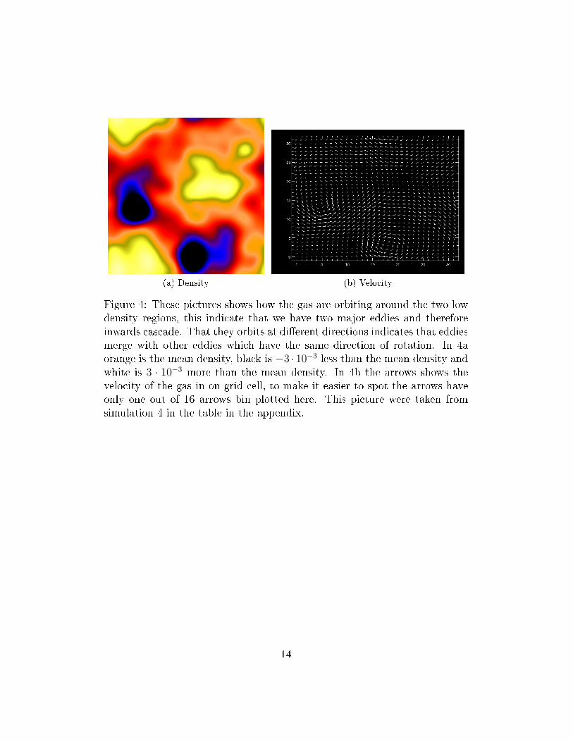
The simulation for the �gures in �gure 4 had the grid size 128, viscosity5 ∗ 10−5 and forced turbulence 0.001, these picture were taken at time 3200.Figure 4a clearly shows how some regions become less dens and some moredens when one has added turbulence to an otherwise homogeneous gas. Onecan see two distinct regions with much less density and if one comparesthat to �gure 4b one will �nd that the gas seems to orbiting around thoseregions. This is what one expect from a simulation where eddies would beable to merge into bigger eddies. The two di�erent regions are orbiting atdi�erent directions, one clockwise and one anticlockwise, indicate that theeddies orbiting in one direction are merging with each other. One also seethat the lowest speed is where the density is highest.

13

(a) Density (b) Velocity

Figure 4: These pictures shows how the gas are orbiting around the two lowdensity regions, this indicate that we have two major eddies and thereforeinwards cascade. That they orbits at di�erent directions indicates that eddiesmerge with other eddies which have the same direction of rotation. In 4aorange is the mean density, black is −3 ·10−3 less than the mean density andwhite is 3 · 10−3 more than the mean density. In 4b the arrows shows thevelocity of the gas in on grid cell, to make it easier to spot the arrows haveonly one out of 16 arrows bin plotted here. This picture were taken fromsimulation 4 in the table in the appendix.

14

(a) Di�erent grid size (b) Di�erent viscosity

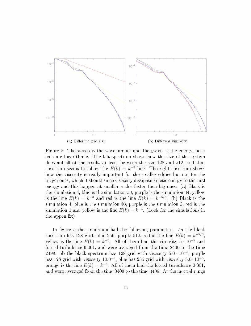
Figure 5: The x-axis is the wavenumber and the y-axis is the energy, bothaxis are logarithmic. The left spectrum shows how the size of the systemdoes not e�ect the result, at least between the size 128 and 512, and thatspectrum seems to follow the E(k) = k−3 line. The right spectrum showshow the viscosity is really important for the smaller eddies but not for thebigger ones, which it should since viscosity dissipate kinetic energy to thermalenergy and this happen at smaller scales faster then big ones. (a) Black isthe simulation 4, blue is the simulation 30, purple is the simulation 34, yellowis the line E(k) = k−3 and red is the line E(k) = k−5/3. (b) Black is thesimulation 4, blue is the simulation 30, purple is the simulation 5, red is thesimulation 1 and yellow is the line E(k) = k−3. (Look for the simulations inthe appendix)

In �gure 5 the simulation had the following parameters. 5a the blackspectrum has 128 grid, blue 256, purple 512, red is the line E(k) = k−5/3,yellow is the line E(k) = k−3. All of them had the viscosity 5 · 10−5 andforced turbulence 0.001, and were averaged from the time 2400 to the time2499. 5b the black spectrum has 128 grid with viscosity 5.0 · 10−5, purplehas 128 grid with viscosity 10.0−5, blue has 256 grid with viscosity 5.0 · 10−5,orange is the line E(k) = k−3. All of them had the forced turbulence 0.001,and were averaged from the time 3400 to the time 3499. At the inertial range

15

one can assume a linear relation between the wavenumber and the energy atthat wavenumber, if one plot them with logarithmic axis. In �gure 6 thesimulations had the following parameters. The black has forced turbulence0.002, blue has forced turbulence 0.001, purple has forced turbulence 0.0005.All of them had the grid size 128 and the viscosity 5 ·10−5, and were averagedfrom the time 2400 to the time 2499. In �gure 5a one can see that the -3line is �tting rather good to the simulations. It is also obvious that theresolution does not matter if the rest of the variables are set to the samevalue. At �gure 5b one see that the viscosity is a variable which matterand that a lower viscosity give higher value for bigger wavenumber, whichmeans that the smaller eddies have more energy. It also gives a indicationthat the simulations come closer to the theoretical line with lower viscositybecause it seems to move closer to the -3 line. Resolution gives a limit forhow small eddies which could be resolved and that the red 64 grid line justend is a consequence of just that. The amount of energy per wavenumbershould be proportional to the amount of forced turbulence and with moreforced turbulence one expect higher energy, which could be seen in �gure 6.It also shows that the shape of the spectrum does almost not change withdi�erent amount of forced turbulence.

16

Figure 6: The x-axis is the wavenumber and the y-axis is the energy, bothaxis are logarithmic. This spectrum shows how the forced turbulence doesnot change the shape of the spectrum but change its position in y directionas it should since there is more energy present with higher forced turbulence.Black is the simulation 7, blue is the simulation 4, purple is the simulation 6and yellow is the line E(k) = k−3.(Look for the simulations in the appendix)

17

(a) Eddies build up (b) Eddies decay

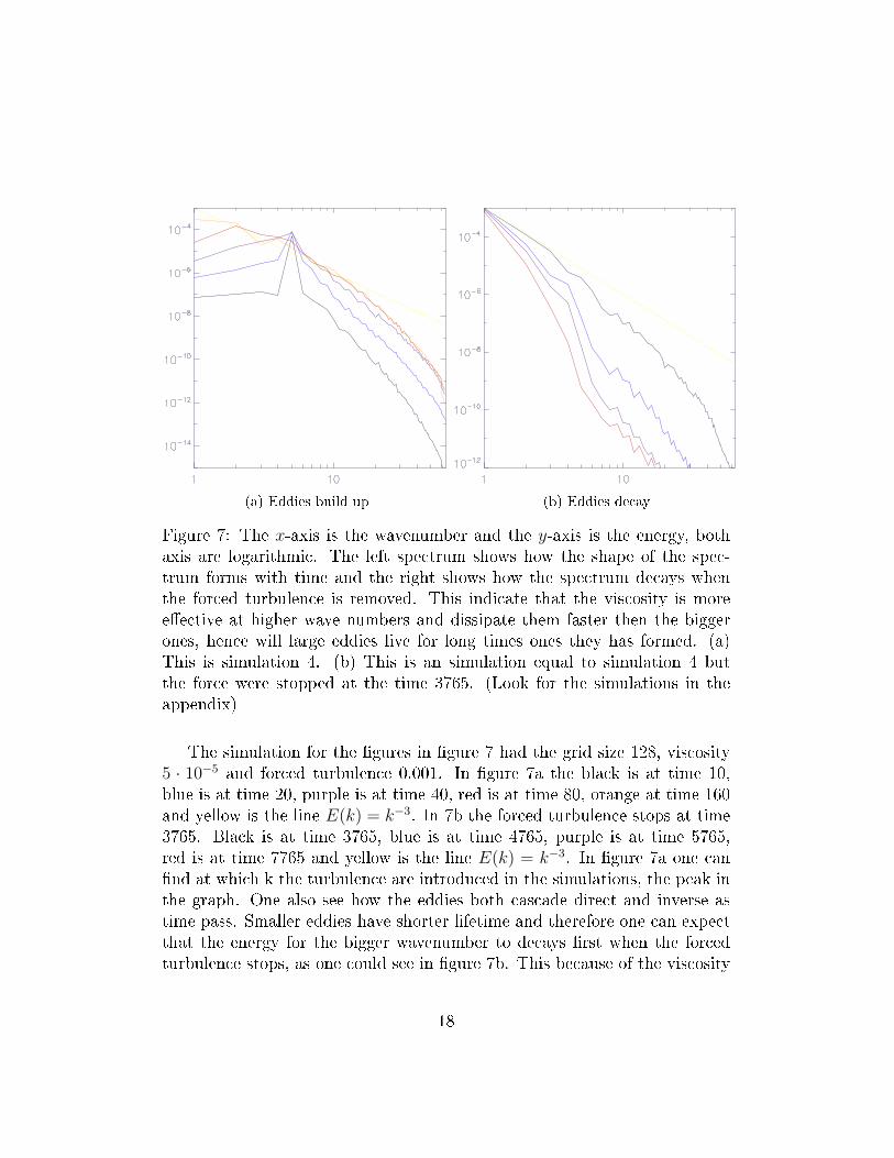
Figure 7: The x-axis is the wavenumber and the y-axis is the energy, bothaxis are logarithmic. The left spectrum shows how the shape of the spec-trum forms with time and the right shows how the spectrum decays whenthe forced turbulence is removed. This indicate that the viscosity is moree�ective at higher wave numbers and dissipate them faster then the biggerones, hence will large eddies live for long times ones they has formed. (a)This is simulation 4. (b) This is an simulation equal to simulation 4 butthe force were stopped at the time 3765. (Look for the simulations in theappendix)

The simulation for the �gures in �gure 7 had the grid size 128, viscosity5 · 10−5 and forced turbulence 0.001. In �gure 7a the black is at time 10,blue is at time 20, purple is at time 40, red is at time 80, orange at time 160and yellow is the line E(k) = k−3. In 7b the forced turbulence stops at time3765. Black is at time 3765, blue is at time 4765, purple is at time 5765,red is at time 7765 and yellow is the line E(k) = k−3. In �gure 7a one can�nd at which k the turbulence are introduced in the simulations, the peak inthe graph. One also see how the eddies both cascade direct and inverse astime pass. Smaller eddies have shorter lifetime and therefore one can expectthat the energy for the bigger wavenumber to decays �rst when the forcedturbulence stops, as one could see in �gure 7b. This because of the viscosity

18

are more e�ective at higher wavenumber, and therefore at smaller eddies.This will cause that large eddies will live very long even if the turbulencestops.

6.2 3D

(a) At time 200 (b) At time 1200

Figure 8: These pictures indicates that the 3D simulations do not have asmuch inverse cascade as the 2D, and already at time 200 does it not seemsto evolve any more. Orange is the mean density, black is −3 · 10−3 less thanthe mean density and white is 3 · 10−3 more than the mean density. The �atplane below the box is the bottom of the box lifted down. This is simulation41. (Look for the simulations in the appendix)

The simulation for the �gures in �gure 8 had the grid size 128, viscosity5 · 10−5 and forced turbulence 0.001. In �gure 9 the black spectrum hadviscosity 5 · 10−5, the blue had viscosity 5 · 10−5, the purple had viscosity5 · 10−5 and yellow is the line E(k) = k−3. All of them had the grid size 128and force turbulence 0.001 and were averaged from the time 900 to the time999. In 3D one does not expect the big inverse cascade as in 2D due to lessmerge between eddies. In �gure 8 one can see that after 200 time frame thegas seems to stop evolve and even if one runs for another 1000 time steps onedo not see any major merge as in 2D. This is what one can expect from a 3Dsimulation and in �gure 9 one see that the energy spectrum does not forma inertial range as in 2D and that the forced turbulence just decay away. It

19

also shows that it merely cascade direct as it decay and the absent of the riseof the bigger eddies. One can also see how higher viscosity are more e�cientto kill of eddies and that smaller eddies are more e�ected by the viscosity.

Figure 9: The x-axis is the wavenumber and the y-axis is the energy, both axisare logarithmic. This spectrum shows how the 3D simulation do not forma initial range and hence one can assume that there is mush less inwardscascade as in 2D. Black is simulation 41, blue is the simulation 42, purple isthe simulation 43 and yellow is the line E(k) = k−3. (Look for the simulationsin the appendix)

20

6.3 Particles

(a) Gas density (b) Particle density

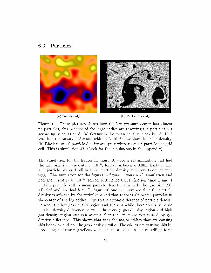
Figure 10: These pictures shows how the low pressure center has almostno particles, this because of the large eddies are throwing the particles outaccording to equation 5. (a) Orange is the mean density, black is −3 · 10−3

less than the mean density and white is 3 · 10−3 more than the mean density.(b) Black means 0 particle density and pure white means 5 particle per gridcell. This is simulation 32. (Look for the simulations in the appendix)

The simulation for the �gures in �gure 10 were a 2D simulation and hadthe grid size 256, viscosity 5 · 10−5, forced turbulence 0.001, friction time1, 1 particle per grid cell as mean particle density and were taken at time2300. The simulation for the �gures in �gure 11 were a 2D simulation andhad the viscosity 5 · 10−5, forced turbulence 0.001, friction time 1 and 1particle per grid cell as mean particle density. 11a hade the gird size 128,11b 256 and 11c had 512. In �gure 10 one can easy see that the particledensity is a�ected by the turbulence and that there is almost no particles inthe center of the big eddies. Due to the strong di�erence of particle densitybetween the low gas density region and the rest while there seems to be noparticle density di�erence between the average gas density region and highgas density region one can assume that the e�ect are not caused by gasdensity di�erence. This shows that it is the major eddies that are causingthis behavior and not the gas density pro�le. The eddies are causing this byproducing a pressure gradient which must be equal to the centrifuge force

21

that push out the particles. In �gure 11 one can see how the maximumparticle density has risen due to this e�ect. In all of them one can see howthe maximum particle density begins at 4 times the mean density and risesto somewhere around 6 and 8 for the mean maximum particle density. Onecan also spot that with higher resolution the maximum tend to get somewhathigher, this is probably because there will be more merges between eddiesin a simulation with higher resolution and this will create more "hot spots"which increase the mean maximum particle density by statistics.

(a) 128 (mmpd 6.03) (b) 256 (mmpd 6.50) (c) 512 (mmpd 7.81)

Figure 11: The x-axis is the time and the y-axis is how many times higher themaximum density is compare to the mean particle density density. Mmpdis the mean maximum particle density. With a higher resolution the maxi-mum particle density slightly increases, this might be due to the increase ofemerging eddies. (a) This is simulation 8. (b) This is simulation 32. (c) Thisis simulation 37. (Look for the simulations in the appendix)

22

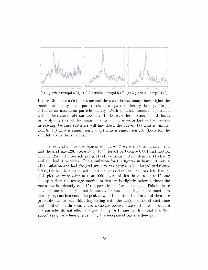
(a) 1 particle (mmpd 6.03) (b) 2 particles (mmpd 5.12) (c) 3 particles (mmpd 4.79)

Figure 12: The x-axis is the time and the y-axis is how many times higher themaximum density is compare to the mean particle density density. Mmpdis the mean maximum particle density. With a higher amount of particleswithin the same resolution does slightly decrease the maximums and this isprobably due to that the maximums do not increases as fast as the mean isincreasing, because statistics will �ne down the curve. (a) This is simula-tion 8. (b) This is simulation 15. (c) This is simulation 16. (Look for thesimulations in the appendix)

The simulation for the �gures in �gure 12 were a 2D simulation andhad the grid size 128, viscosity 5 · 10−5, forced turbulence 0.001 and frictiontime 1. 12a had 1 particle per grid cell as mean particle density, 11b had 2and 11c had 3 particles. The simulation for the �gures in �gure 13 were a2D simulation and had the grid size 128, viscosity 5 · 10−5, forced turbulence0.001, friction time 1 and had 1 particle per grid cell as mean particle density.This pictures were taken at time 1000. In all of this three, in �gure 12, onecan spot that the average maximum density is slightly below 6 times themean particle density even if the particle density is changed. This indicatethat the mean density is not impotent for how much higher the maximumdensity regions become. The peak at about the time 1000 in all of them areprobable due to something happening with the major eddies at that timeand in all of this three simulations the gas behaves exactly the same becausethe particles do not e�ect the gas. In �gure 13 one can �nd that the "hotspots" region is where one can �nd the increase of particle density.

23

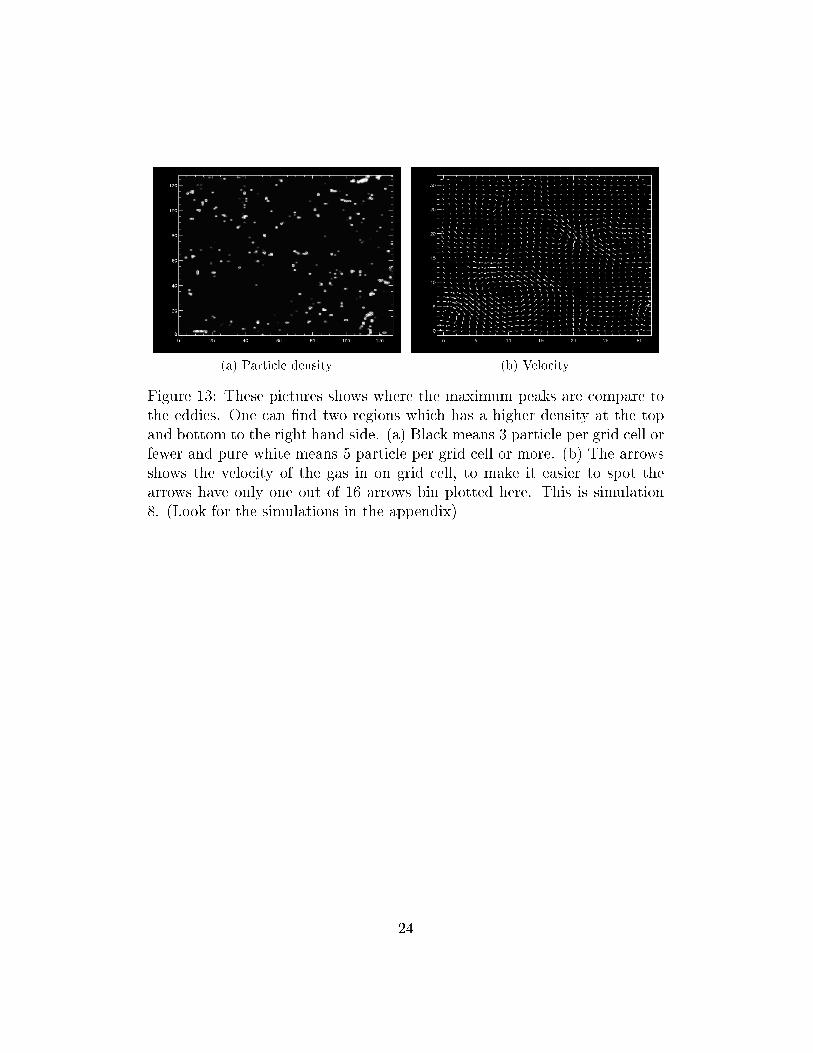
(a) Particle density (b) Velocity

Figure 13: These pictures shows where the maximum peaks are compare tothe eddies. One can �nd two regions which has a higher density at the topand bottom to the right hand side. (a) Black means 3 particle per grid cell orfewer and pure white means 5 particle per grid cell or more. (b) The arrowsshows the velocity of the gas in on grid cell, to make it easier to spot thearrows have only one out of 16 arrows bin plotted here. This is simulation8. (Look for the simulations in the appendix)

24

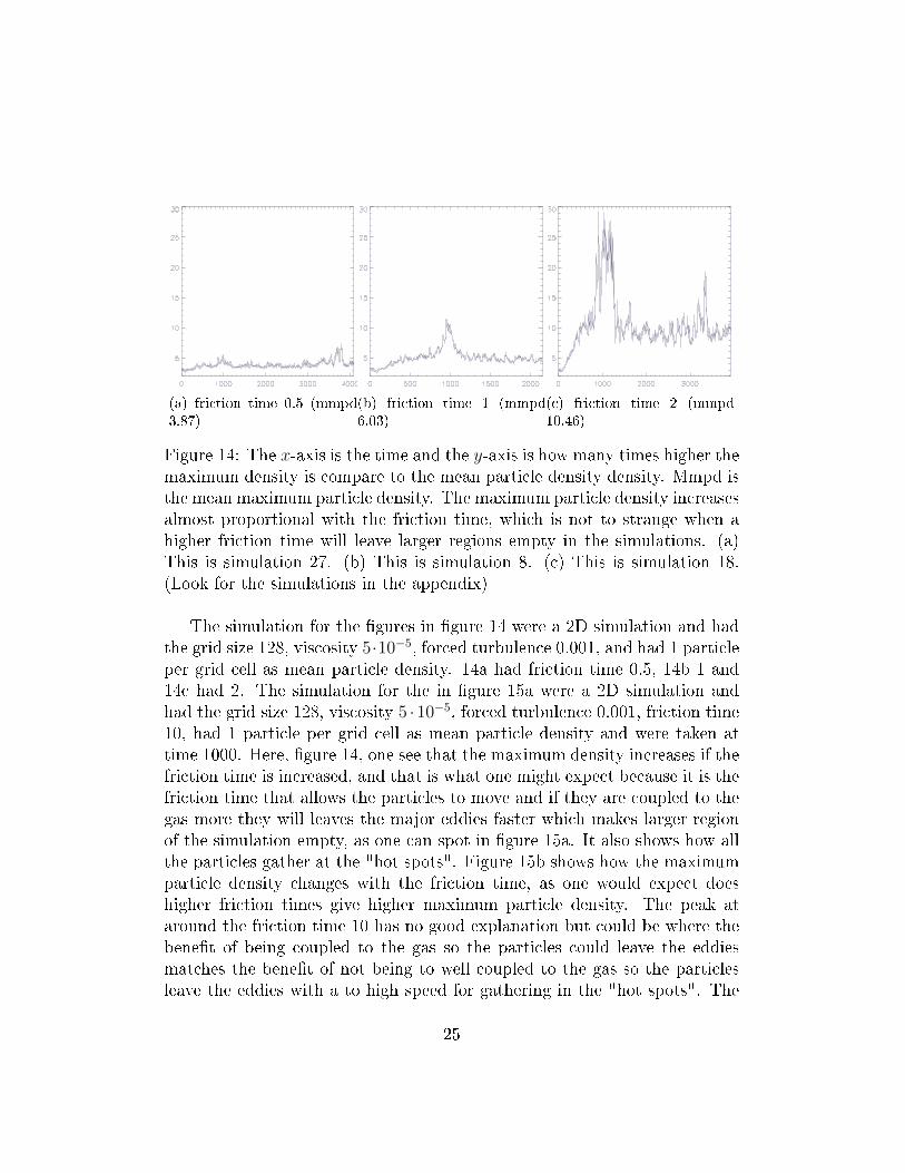
(a) friction time 0.5 (mmpd3.87)

(b) friction time 1 (mmpd6.03)

(c) friction time 2 (mmpd10.46)

Figure 14: The x-axis is the time and the y-axis is how many times higher themaximum density is compare to the mean particle density density. Mmpd isthe mean maximum particle density. The maximum particle density increasesalmost proportional with the friction time, which is not to strange when ahigher friction time will leave larger regions empty in the simulations. (a)This is simulation 27. (b) This is simulation 8. (c) This is simulation 18.(Look for the simulations in the appendix)

The simulation for the �gures in �gure 14 were a 2D simulation and hadthe grid size 128, viscosity 5·10−5, forced turbulence 0.001, and had 1 particleper grid cell as mean particle density. 14a had friction time 0.5, 14b 1 and14c had 2. The simulation for the in �gure 15a were a 2D simulation andhad the grid size 128, viscosity 5 ·10−5, forced turbulence 0.001, friction time10, had 1 particle per grid cell as mean particle density and were taken attime 1000. Here, �gure 14, one see that the maximum density increases if thefriction time is increased, and that is what one might expect because it is thefriction time that allows the particles to move and if they are coupled to thegas more they will leaves the major eddies faster which makes larger regionof the simulation empty, as one can spot in �gure 15a. It also shows how allthe particles gather at the "hot spots". Figure 15b shows how the maximumparticle density changes with the friction time, as one would expect doeshigher friction times give higher maximum particle density. The peak ataround the friction time 10 has no good explanation but could be where thebene�t of being coupled to the gas so the particles could leave the eddiesmatches the bene�t of not being to well coupled to the gas so the particlesleave the eddies with a to high speed for gathering in the "hot spots". The

25

�gure also shows that the random noise in this simulations is almost 4 inmean maximum particle density.

(a) Particle density (b) Meanmax function

Figure 15: The left hand side plot shows how the big regions become emptywhen one increases the friction time and at the value 10 the particle arealmost only distributed along the "hot spots". The right hand side plotshows how the maximum particle density changes with the friction time, onecan assume a maximum somewhere around the friction time 10. (a) Blackmeans 0 particle per grid cell and pure white means 100 particle per grid cell.(b) This is a plot of the average maximum particle density as a function ofthe friction time. x-axis is the friction time and y-axis is the mean maximumparticle density, and both axis are logarithmic. This is simulation 21. (Lookfor the simulations in the appendix)

26

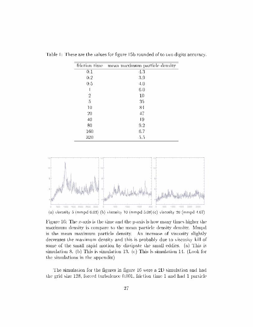
Table 1: These are the values for �gure 15b rounded of to two digits accuracy.

friction time mean maximum particle density0.1 4.30.2 3.90.5 4.01 6.02 105 3510 8420 4740 1980 9.2160 6.7320 5.5

(a) viscosity 5 (mmpd 6.03) (b) viscosity 10 (mmpd 5.08)(c) viscosity 20 (mmpd 4.67)

Figure 16: The x-axis is the time and the y-axis is how many times higher themaximum density is compare to the mean particle density density. Mmpdis the mean maximum particle density. An increase of viscosity slightlydecreases the maximum density and this is probably due to viscosity kill ofsome of the small rapid motion by dissipate the small eddies. (a) This issimulation 8. (b) This is simulation 13. (c) This is simulation 14. (Look forthe simulations in the appendix)

The simulation for the �gures in �gure 16 were a 2D simulation and hadthe grid size 128, forced turbulence 0.001, friction time 1 and had 1 particle

27

per grid cell as mean particle density. 16a had the viscosity 5 ·10−5, 16b 10−4

and 16c had 2 · 10−4. The small chance of maximum density in �gure 16 canbe explained by less merge of smaller eddies, due to higher viscosity dissipatesmore smaller eddies e �gure 5, which then creates fewer "hot spots", and withfewer "hot spots" there will be less chance of getting a very high maximum,due to statistics. But the major increase in the maximum particle densityis produced by the major eddies and the viscosity are not changing energyspectrum for the large eddies and therefore will there still be an increase inmaximum particle density.

(a) force 0.0005 (mmpd 4.42) (b) force 0.001 (mmpd 6.03) (c) force 0.002 (mmpd 8.01)

Figure 17: The x-axis is the time and the y-axis is how many times higher themaximum density is compare to the mean particle density density. Mmpdis the mean maximum particle density. An increase in the forced turbulencewill result in an increase of the particle density, which is what one expectwhen one adds more turbulence into the simulation. (a) This is simulation11. (b) This is simulation 15. (c) This is simulation 12. (Look for thesimulations in the appendix)

The simulation for the �gures in �gure 17 were a 2D simulation and hadthe grid size 128, viscosity 5∗10−5, friction time 1 and had 2 particle per gridcell as mean particle density. 17a had forced turbulence 0.0005, 17b 0.001and 17c had 0.002. The increase of maximum particle density goes up withan increasing forced turbulence is quite straight forward, more turbulencewill cause higher kinetic energy which can create motion to the particles sothey could gather into higher concentration.

28

(a) 2D (mmpd 4.73) (b) 3D (mmpd 4.30)

Figure 18: The x-axis is the time and the y-axis is how many times higher themaximum density is compare to the mean particle density density. Mmpdis the mean maximum particle density. These has a really low maximumparticle density so one should not trust them completely. But it seems thatthe 2D has somewhat higher maximum particle density, which one can expectdue to the reduced amount of inverse cascade. (a) This is simulation 3. (b)This is simulation 40. (Look for the simulations in the appendix)

The simulation for the �gures in �gure 18 had the grid size 64, viscosity2 · 10−4, forced turbulence 0.001, friction time 2 and had 1 particle per gridcell as mean particle density. 18a were a 2D simulation and 18b were a 3D.In �gure 18 one can see that the height of the maximum particle density isslightly higher in the 2D simulation, but it is not so clear that one can stateit. A problem is that the 64 resolution is so small that the background noiseis almost almost as big as the expected result, because lower resolution giveslower maximum density (see �gure 11). The fact that the 3D simulation has64 times as many particles as the 2D should not be a problem accordingto �gure 12. The increased viscosity is also a problem according to �gure20, which state that higher viscosity gives slightly lower maximum particledensity. All this factors working together are probably the reason why it is sohard to read out anything from this. But one can see a slight increase in the2D simulation, which is what one would expect from this kind of simulation.The increase is an e�ect from the lack of inverse cascade in the 3D simulationscompare to the 2D simulations.

29

7 Conclusion

When one changed the the grid size for the simulations but kept all otherparameters �xed the spectrum did not change. This tell one that the resolu-tion is not an important property of the eddies. If one changed the viscosityone would see that the small eddies gained much less energy, which indicatethat the smaller eddies are stronger e�ected by the viscosity. It did alsoshow how less viscosity seemed to make the inertial range move to smallereddies and closer to the E(k) = k−3 line. The amount of forced turbulencedo not change the shape of the spectrum but an increase of turbulence givean increase kinetic energy and the spectrum is forming throw inverse anddirect cascade. This shows how the forced turbulence is important for theamount of eddies that forms but not their properties. By looking at how theforced turbulence change the spectrum early in the simulations one can seethat the 2D clearly has both inverse and direct cascade. When the forcedturbulence stops one can �nd how the viscosity dissipate the small eddiesmuch more e�ective than the large eddies, which will result in that largeeddies will last much longer and would therefore be a better candidate forplanetesimal formation than small eddies. The 3D simulation did not haveany major inverse cascade which one can expect from a 3D simulation wherethe merge of eddies is much less likely. This resulted in a spectrum with-out any inertial range and therefore no major eddies swirling around for anylong time, one could �nd that it only took until the time 200 before the 3Dsimulation stopped to evolve.

The particle simulation showed that the large eddies were e�ective formaking large regions with low particle density, which makes the large eddiesto a candidate for planetesimal formation. An increase viscosity did slightlyreduce the mean maximum particle density, which can be explained by alittle less of the smaller eddies which will give little fewer "hot spots". Anincrease of the resolution did slightly increase the mean maximum particledensity, which can be explained by somewhat more "hot spots". An increaseof particle number did slightly reduce the mean maximum particle density,which can be explained by a lower random noise. The only 3D simulation Imade and its comparable 2D simulation did both have mean maximum parti-cle density to close to the random noise to make any reliable statement. Theonly two variables which had any major e�ect on the increase of maximumparticle density were the friction time and the amount of forced turbulence.That an increase of forced turbulence will give an increase of the mean max-

30

imum particle density is because it will have more energy along all sizes ofeddies, which include the ones who creates the particle density to increaseabove the mean particle density. The big peak of mean maximum particledensity around the friction time 10 is really an interesting result, this bothshows that if turbulence are present in a protoplanetary disk the turbulencewill contribute to get higher particle density which might create planetesimaland it also indicate that the most important property is the friction time.

Their are several aspect that would be interesting to look into if I hadmore time. The �rst and most obvious is the peak in the mean maximumparticle density around the friction time 10. I would concentrate to look ifI could �nd more behavior like this for di�erent viscosity, grid size, forcedturbulence and amount of particles. One could also try to �nd out whetherany kind of 3D simulation could show any similar behavior.

31

8 References

Burden Tony, 2008, [http://www2.mech.kth.se/courses/5C1218/scales.pdf]

Cuzzi N. Je�rey, Hogan C. Robert, Paque M. Julie, Dobrovolskis R. An-thony, 2001, Astrophysical Journal, vol. 546, p. 496-508

Dominik C., Blum J., Cuzzi J., Wurm G., 2006, [http://arxiv.org/pdf/astro-ph/0602617v1.pdf]

Elaine S.Oran, Jay P.Boris, 1987, Numerical simulations of reactive �ows,�fth edition, p. 161

Frisch Uriel, 1995, Turbulence, p. 1

Kraichnan H. Robert, 1967, Physics of Fluids, Vol. 10, p.1417-1423

Lundgren T. S., 2003, [http://ctr.stanford.edu/ResBriefs03/lundgren.pdf]

Manneville Paul, 2004, Instabilities, chaos and turbulence, p. 271

Markiewicz, W. J., Mizuno, H., Voelk, H. J., 1991, Astronomy and Astro-physics, vol. 242, p. 286-289

O'dell, C. R., Wen, Z., Hu, X, 1993, Astrophysical Journal, vol. 410, no.2, p. 696-700

Philip J. Armitage, 2010, Astrophysics of Planet Formation, Cambridge Uni-versity Press, version 3

Wallace M john, Hobbs V Perer, 2006, atmospheric science an introductorysurvey, p. 13

32

9 Appendix

Table 2: All the simulation that I have done during my bachelor project.Where mpd stands for the mean particle density and τ stands for the frictiontime. All this simulation were made in 2D.

number grid size viscosity forced turbulence τ mean particle density1 64 10 0.001 - -2 64 20 0.001 1 13 64 20 0.001 2 14 128 5 0.001 - -5 128 10 0.001 - -6 128 5 0.0005 - -7 128 5 0.002 - -8 128 5 0.001 1 19 128 5 0.0005 1 110 128 5 0.002 1 111 128 5 0.0005 1 212 128 5 0.002 1 213 128 10 0.001 1 114 128 20 0.001 1 115 128 5 0.001 1 216 128 5 0.001 1 317 128 5 0.001 1 518 128 5 0.001 2 119 128 5 0.001 2 220 128 5 0.001 5 121 128 5 0.001 10 122 128 5 0.001 20 123 128 5 0.001 40 124 128 5 0.001 80 125 128 5 0.001 160 126 128 5 0.001 320 127 128 5 0.001 0.5 128 128 5 0.001 0.2 129 128 5 0.001 0.1 1

33

Table 3: All the simulation that I have done during my bachelor project.Where mpd stands for the mean particle density and τ stands for the frictiontime. The simulation 30− 37 were in 2D and 38− 43 were in 3D.

number grid size viscosity forced turbulence τ mean particle density30 256 5 0.001 - -31 256 2.5 0.001 - -32 256 5 0.001 1 133 256 2.5 0.001 1 134 512 5 0.001 - -35 512 2.5 0.001 - -36 512 1.25 0.001 - -37 512 5 0.001 1 138 64 20 0.001 - -39 64 20 0.001 1 140 64 20 0.001 2 141 128 5 0.001 - -42 128 10 0.001 - -43 128 20 0.001 - -

34