tube wave to shear wave conversion at borehole...

Geophysical Prospecting doi: 10.1111/1365-2478.12095

Tube wave to shear wave conversion at borehole plugsTim Seher1∗, Stephane Rondenay2 and Hugues Djikpesse3,4

1Formerly at: Earth Resources Laboratory, Massachusetts Institute of Technology, 77 Massachusetts Avenue, Cambridge, MA 02139-4307,U.S.A., 2University of Bergen – Department of Earth Science, Bergen, Norway, 3Schlumberger-Doll Research, Cambridge, Massachusetts,United States, and 4Visiting Scientist, Energy Initiatives, Massachusets Institute of Technology, Cambridge, MA, U.S.A.

Received September 2012, revision accepted June 2013

ABSTRACTIn hydraulic fracturing experiments, perforation shots excite body and tube wavesthat sample, and thus can be used to characterize, the surrounding medium. Whilethese waves are routinely employed in borehole operations, their resolving poweris limited by the experiment geometry, the signal-to-noise ratio, and their frequencycontent. It is therefore useful to look for additional, complementary signals that couldincrease this resolving power. Tube-to-body-wave conversions (scattering of tube tocompressional or shear waves at borehole discontinuities) are one such signal. Thesewaves are not frequently considered in hydraulic fracture settings, yet they possessgeometrical and spectral attributes that greatly complement the resolution afforded bybody and tube waves alone. Here, we analyze data from the Jonah gas field (Wyoming,USA) to demonstrate that tube-to-shear-wave conversions can be clearly observed inthe context of hydraulic fracturing experiments. These waves are identified primarilyon the vertical and radial components of geophones installed in monitoring wellssurrounding a treatment well. They exhibit a significantly lower frequency content(10–100 Hz) than the primary compressional waves (100–1000 Hz). Tapping intosuch lower frequencies could help to better constrain velocity in the formation, thusallowing better estimates of fracture density, porosity and permeability. Moreover,the signals of tube-to-shear-wave conversion observed in this particular study provideindependent estimates of the shear wave velocity in the formation and of the tubewave velocity in the treatment well.

Key words: Seismics, Wave, Borehole geophysics, Monitoring.

1 INTRODUCT I ON

Traditionally, exploration seismologists have mainly usedreflected and refracted seismic body waves for subsurfacecharacterization. However, an increase in seismic borehole ex-periments and improved instrumentation have allowed the ob-servation of other useful, albeit less common waves (Fig. 1a).These include conversions from tube to shear waves – the fo-cus of this study – which provide additional resolving powerthat can advance the understanding of the subsurface.

Tube waves, which propagate along the borehole, mayemanate from seismic sources located inside the borehole.

∗E-mail: [email protected]

Whenever there are obstacles within the borehole, tube wavesmay be converted to body waves (either compressional orshear waves). Such conversions have been observed in situa-tions where a tube wave reaches the bottom of the borehole,or where a tube wave impinges upon open fractures or irreg-ularities in the borehole wall (White and Sengbush 1963; Leeet al. 1984; Beydoun et al. 1985; Hardage 2000; Greenhalghet al. 2000, 2003; Xu and Greenhalgh 2010). In particular,tube-to-body-wave conversions have been exploited as sec-ondary sources for borehole seismic experiments (Norris andAronstam 2003; Aronstam 2004). Similar reciprocal conver-sions from body to tube wave may occur when a body wavepasses through a borehole.

C© 2014 European Association of Geoscientists & Engineers 1

2 T. Seher, S. Rondenay and H. Djikpesse

2 3 4 5Velocity (km/s)

600

560

520

Dep

th (m

)

1

2

3

4

5

6

7

8

9

11

10

Plug

1

3

4

5

6

2

0 40 80 120Offset (m)

600

560

520

Dep

th (m

)

Receiverarray

Perforation shots

A

4

3

2

1

Treatmentwell

Monitoringwell

Plug Bottom reflector

Top reflector

B

P-waveS-wave

(a)

(b)

(c)

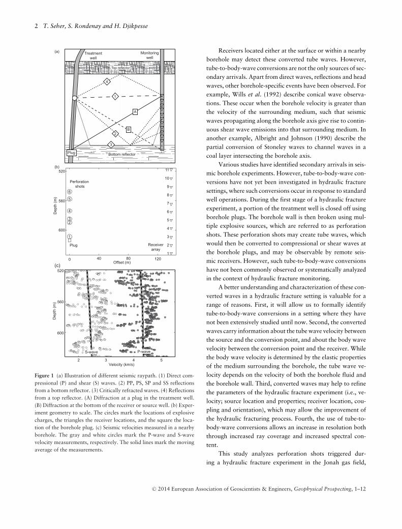
Figure 1 (a) Illustration of different seismic raypath. (1) Direct com-pressional (P) and shear (S) waves. (2) PP, PS, SP and SS reflectionsfrom a bottom reflector. (3) Critically refracted waves. (4) Reflectionsfrom a top reflector. (A) Diffraction at a plug in the treatment well.(B) Diffraction at the bottom of the receiver or source well. (b) Exper-iment geometry to scale. The circles mark the locations of explosivecharges, the triangles the receiver locations, and the square the loca-tion of the borehole plug. (c) Seismic velocities measured in a nearbyborehole. The gray and white circles mark the P-wave and S-wavevelocity measurements, respectively. The solid lines mark the movingaverage of the measurements.

Receivers located either at the surface or within a nearbyborehole may detect these converted tube waves. However,tube-to-body-wave conversions are not the only sources of sec-ondary arrivals. Apart from direct waves, reflections and headwaves, other borehole-specific events have been observed. Forexample, Wills et al. (1992) describe conical wave observa-tions. These occur when the borehole velocity is greater thanthe velocity of the surrounding medium, such that seismicwaves propagating along the borehole axis give rise to contin-uous shear wave emissions into that surrounding medium. Inanother example, Albright and Johnson (1990) describe thepartial conversion of Stoneley waves to channel waves in acoal layer intersecting the borehole axis.

Various studies have identified secondary arrivals in seis-mic borehole experiments. However, tube-to-body-wave con-versions have not yet been investigated in hydraulic fracturesettings, where such conversions occur in response to standardwell operations. During the first stage of a hydraulic fractureexperiment, a portion of the treatment well is closed off usingborehole plugs. The borehole wall is then broken using mul-tiple explosive sources, which are referred to as perforationshots. These perforation shots may create tube waves, whichwould then be converted to compressional or shear waves atthe borehole plugs, and may be observable by remote seis-mic receivers. However, such tube-to-body-wave conversionshave not been commonly observed or systematically analyzedin the context of hydraulic fracture monitoring.

A better understanding and characterization of these con-verted waves in a hydraulic fracture setting is valuable for arange of reasons. First, it will allow us to formally identifytube-to-body-wave conversions in a setting where they havenot been extensively studied until now. Second, the convertedwaves carry information about the tube wave velocity betweenthe source and the conversion point, and about the body wavevelocity between the conversion point and the receiver. Whilethe body wave velocity is determined by the elastic propertiesof the medium surrounding the borehole, the tube wave ve-locity depends on the velocity of both the borehole fluid andthe borehole wall. Third, converted waves may help to refinethe parameters of the hydraulic fracture experiment (i.e., ve-locity; source location and properties; receiver location, cou-pling and orientation), which may allow the improvement ofthe hydraulic fracturing process. Fourth, the use of tube-to-body-wave conversions allows an increase in resolution boththrough increased ray coverage and increased spectral con-tent.

This study analyzes perforation shots triggered dur-ing a hydraulic fracture experiment in the Jonah gas field,

C© 2014 European Association of Geoscientists & Engineers, Geophysical Prospecting, 1–12

Tube wave to shear wave conversion 3

situated in the Rocky Mountains region of Wyoming – oneof the largest onshore natural gas discoveries in the UnitedStates (Robinson and Shanley 2005). The focus of this arti-cle is on the observation of tube-to-body wave conversions.Therefore, the methodology used to test for the origin of theobserved signal is detailed in appendices A, B, and C. In thenext section, we concentrate on the validation and physical in-terpretation of this observation. The seismograms associatedwith the perforation shots exhibit strong secondary seismicarrivals. Here, we explore different explanations for thosearrivals and demonstrate that the most likely explanation istube-to-shear-wave scattering at plugs in the treatment well.Based on this result, we derive a simple method for calibratingthe tube wave velocity in the treatment well that provides newinsights in the low frequency behaviour of tube waves. Weconclude by discussing the properties and possible future usesof the tube-to-shear-wave scattered signal.

2 OBSERVATION S A N D A N A L Y SI S

The seismic wave created by a single source usually containsinformation beyond compressional and shear wave arrivals,which is rarely exploited completely. This is often linked todifficulties in assigning parts of the seismic coda to a uniqueorigin. However, if a part of the seismic coda has been success-fully identified, it usually advances the understanding of thesubsurface. Here, we commence our analysis by presentingobservations of both primary and secondary arrivals. Thenwe investigate a range of possible mechanisms to explain theorigin of the secondary arrivals, and use independent obser-vations from microearthquakes to validate our choice of pre-ferred mechanism.

2.1 Observations from perforation shots

We examine the seismograms created by perforation shotsdetonated during one stage of a hydraulic fracture experimentin the Jonah Field. As part of this experiment, six explosivecharges were detonated in a treatment well ∼138 m from aparallel monitoring well (Fig. 1b). The seismic arrivals causedby the explosives were observed on an array of eleven three-component receivers spaced ∼11–12 m apart. For simplicity,the three component records (East, North and vertical) wererotated to align one of the horizontal components with thesource receiver plane (radial, transverse and vertical). Afterrotation, the energy of a compressional wave caused by aperforation shot is detected on the radial and vertical compo-nents of the receivers only. For completeness, the processing

sequence for hydraulic fracture monitoring is summarized inappendix A.

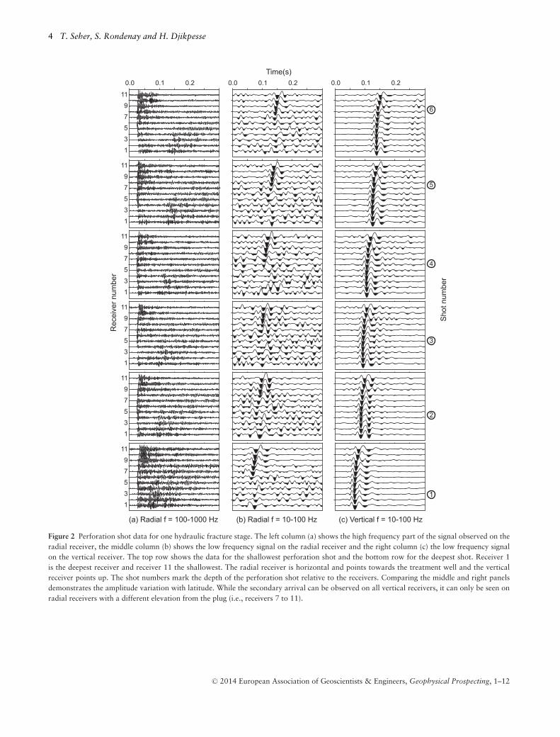
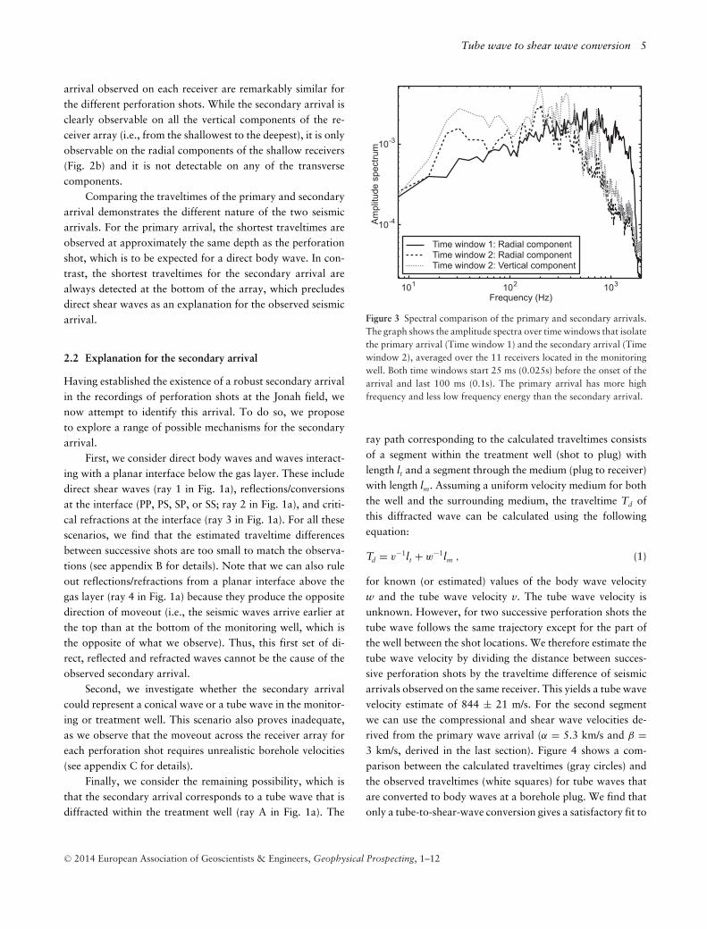
The observed seismograms are dominated by two seismicarrivals that exhibit significantly different frequency contents(Fig. 2). We also note the presence of a third, weak arrival,that is not analyzed in this study (shots 5 and 6 in Fig. 2c).The first arrival, observed at traveltimes between ∼22–33ms, dominates in the high-frequency portion of the signal(0.1–1 kHz). This contrasts with the second arrival, which isobserved at traveltimes between ∼50–135 ms and dominatesin the low-frequency portion of the seismogram (10–100 Hz).The difference in frequency content between the two arrivals isalso clearly observed when comparing their respective spectra(see Fig. 3). In Fig. 3 two time windows with a length of 100ms are used to select the two different arrivals. Time window1 selects the primary wave energy on the radial component(compare Fig. 2a) and time window 2 selects the secondarywave energy on both the radial and vertical component (com-pare Figs 2b and 2c).

The high frequency signal corresponds to the direct com-pressional wave arrival. It is strongest on the radial component(Fig. 2a), and it is not observed on the transverse component.Assuming an isotropic medium, the observed traveltimes indi-cate a primary wave velocity of 5.3 ± 0.1 km/s. These veloc-ities are ∼1 km/s faster than the average compressional wavevelocities measured in a borehole located 470 m away fromthe hydraulic fracture area (Fig. 2c; well log velocities pro-vided courtesy of Encana). This velocity difference is largerthan the variability in the well log velocities. Maxwell et al.(2006) observed a traveltime variation with incidence anglefor perforation shot records and proposed seismic anisotropyas a possible explanation for the difference between verticalvelocities and horizontal perforation shot velocities. We stressthat this velocity variability cannot explain the traveltime dif-ferences analyzed in this study. Finally, the primary wave ve-locity can be used to estimate the shear wave velocity, using aVp/Vs ratio of ∼1.7 derived from the borehole measurements.This gives a shear wave velocity of ∼3.0 km/s.

The secondary, low frequency arrival is clearest on thevertical component (Fig. 2c) and its absolute traveltimes varywith shot depth. The shallowest shot (shot 6 in Fig. 2) cor-responds to the longest traveltimes (∼120–135 ms) whereasthe deepest shot (shot 1 in Fig. 2) produces the shortest travel-times (∼50–63 ms). From the perspective of the receiver array,we note that the secondary arrivals follow an identical rela-tive moveout curve from one perforation shot to another (i.e.,the traveltimes with their mean removed are approximatelyidentical). We further note that the wavelets of the secondary



1

3

5

7

9

11

1

3

5

7

9

11

1

3

5

7

9

11

1

3

5

7

9

11

1

3

5

7

9

11

1

3

5

7

9

11

0.0 0.1 0.2 0.0 0.1 0.2 0.0 0.1 0.2Time(s)

(a) Radial f = 100-1000 Hz (b) Radial f = 10-100 Hz (c) Vertical f = 10-100 Hz

1

2

3

4

5

6R

ecei

ver n

umbe

r

Sho

t num

ber

Figure 2 Perforation shot data for one hydraulic fracture stage. The left column (a) shows the high frequency part of the signal observed on theradial receiver, the middle column (b) shows the low frequency signal on the radial receiver and the right column (c) the low frequency signalon the vertical receiver. The top row shows the data for the shallowest perforation shot and the bottom row for the deepest shot. Receiver 1is the deepest receiver and receiver 11 the shallowest. The radial receiver is horizontal and points towards the treatment well and the verticalreceiver points up. The shot numbers mark the depth of the perforation shot relative to the receivers. Comparing the middle and right panelsdemonstrates the amplitude variation with latitude. While the secondary arrival can be observed on all vertical receivers, it can only be seen onradial receivers with a different elevation from the plug (i.e., receivers 7 to 11).



arrival observed on each receiver are remarkably similar forthe different perforation shots. While the secondary arrival isclearly observable on all the vertical components of the re-ceiver array (i.e., from the shallowest to the deepest), it is onlyobservable on the radial components of the shallow receivers(Fig. 2b) and it is not detectable on any of the transversecomponents.

Comparing the traveltimes of the primary and secondaryarrival demonstrates the different nature of the two seismicarrivals. For the primary arrival, the shortest traveltimes areobserved at approximately the same depth as the perforationshot, which is to be expected for a direct body wave. In con-trast, the shortest traveltimes for the secondary arrival arealways detected at the bottom of the array, which precludesdirect shear waves as an explanation for the observed seismicarrival.

2.2 Explanation for the secondary arrival

Having established the existence of a robust secondary arrivalin the recordings of perforation shots at the Jonah field, wenow attempt to identify this arrival. To do so, we proposeto explore a range of possible mechanisms for the secondaryarrival.

First, we consider direct body waves and waves interact-ing with a planar interface below the gas layer. These includedirect shear waves (ray 1 in Fig. 1a), reflections/conversionsat the interface (PP, PS, SP, or SS; ray 2 in Fig. 1a), and criti-cal refractions at the interface (ray 3 in Fig. 1a). For all thesescenarios, we find that the estimated traveltime differencesbetween successive shots are too small to match the observa-tions (see appendix B for details). Note that we can also ruleout reflections/refractions from a planar interface above thegas layer (ray 4 in Fig. 1a) because they produce the oppositedirection of moveout (i.e., the seismic waves arrive earlier atthe top than at the bottom of the monitoring well, which isthe opposite of what we observe). Thus, this first set of di-rect, reflected and refracted waves cannot be the cause of theobserved secondary arrival.

Second, we investigate whether the secondary arrivalcould represent a conical wave or a tube wave in the monitor-ing or treatment well. This scenario also proves inadequate,as we observe that the moveout across the receiver array foreach perforation shot requires unrealistic borehole velocities(see appendix C for details).

Finally, we consider the remaining possibility, which isthat the secondary arrival corresponds to a tube wave that isdiffracted within the treatment well (ray A in Fig. 1a). The

101

Frequency (Hz)102 103

Am

plitu

de s

pect

rum10-3

10-4

Time window 1: Radial componentTime window 2: Radial componentTime window 2: Vertical component

Figure 3 Spectral comparison of the primary and secondary arrivals.The graph shows the amplitude spectra over time windows that isolatethe primary arrival (Time window 1) and the secondary arrival (Timewindow 2), averaged over the 11 receivers located in the monitoringwell. Both time windows start 25 ms (0.025s) before the onset of thearrival and last 100 ms (0.1s). The primary arrival has more highfrequency and less low frequency energy than the secondary arrival.

ray path corresponding to the calculated traveltimes consistsof a segment within the treatment well (shot to plug) withlength lt and a segment through the medium (plug to receiver)with length lm. Assuming a uniform velocity medium for boththe well and the surrounding medium, the traveltime Td ofthis diffracted wave can be calculated using the followingequation:

Td = v−1lt + w−1lm , (1)

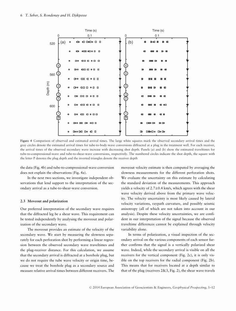
for known (or estimated) values of the body wave velocityw and the tube wave velocity v. The tube wave velocity isunknown. However, for two successive perforation shots thetube wave follows the same trajectory except for the part ofthe well between the shot locations. We therefore estimate thetube wave velocity by dividing the distance between succes-sive perforation shots by the traveltime difference of seismicarrivals observed on the same receiver. This yields a tube wavevelocity estimate of 844 ± 21 m/s. For the second segmentwe can use the compressional and shear wave velocities de-rived from the primary wave arrival (α = 5.3 km/s and β =3 km/s, derived in the last section). Figure 4 shows a com-parison between the calculated traveltimes (gray circles) andthe observed traveltimes (white squares) for tube waves thatare converted to body waves at a borehole plug. We find thatonly a tube-to-shear-wave conversion gives a satisfactory fit to



0 0.1Time (s)

1

23

4

5

6

P

0 0.1

600

560

520D

epth

(m)

Time (s)

1

23

4

5

6

P

(a) (b)

Figure 4 Comparison of observed and estimated arrival times. The large white squares mark the observed secondary arrival times and thegray circles denote the estimated arrival times for tube-to-body-wave conversions diffracted at a plug in the treatment well. For each receiver,the arrival times of the observed secondary wave increase with decreasing shot depth. Panels (a) and (b) show the estimated traveltimes fortube-to-compressional-wave and tube-to-shear-wave conversions, respectively. The numbered circles indicate the shot depth, the square withthe letter P denotes the plug depth and the inverted triangles denote the receiver depth

the data (Fig. 4b) and tube-to-compressional-wave conversiondoes not explain the observations (Fig. 4a).

In the next two sections, we investigate independent ob-servations that lend support to the interpretation of the sec-ondary arrival as a tube-to-shear-wave conversion.

2.3 Moveout and polarization

Our preferred interpretation of the secondary wave requiresthat the diffracted leg be a shear wave. This requirement canbe tested independently by analysing the moveout and polar-ization of the secondary wave.

The moveout provides an estimate of the velocity of thesecondary wave. We start by measuring the slowness sepa-rately for each perforation shot by performing a linear regres-sion between the observed secondary wave traveltimes andthe plug-receiver distance. For this calculation, we assumethat the secondary arrival is diffracted at a borehole plug, butwe do not require the tube wave velocity or origin time, be-cause we treat the borehole plug as a secondary source andmeasure relative arrival times between different receivers. The

moveout velocity estimate is then computed by averaging theslowness measurements for the different perforation shots.We evaluate the uncertainty on this estimate by calculatingthe standard deviation of the measurements. This approachyields a velocity of 2.7±0.4 km/s, which agrees with the shearwave velocity derived above from the primary wave veloc-ity. The velocity uncertainty is most likely caused by lateralvelocity variations, raypath curvature, and possibly seismicanisotropy (all of which are not taken into account in ouranalysis). Despite these velocity uncertainties, we are confi-dent in our interpretation of the signal because the observedtraveltime differences cannot be explained through velocityvariability alone.

In terms of polarization, a visual inspection of the sec-ondary arrival on the various components of each sensor fur-ther confirms that the signal is a vertically polarized shearwave. Indeed, while the secondary arrival is visible on all thereceivers for the vertical component (Fig. 2c), it is only vis-ible on the top receivers for the radial component (Fig. 2b).This means that for receivers located at a depth similar tothat of the plug (receivers 2&3, Fig. 2), the shear wave travels



1

3

5

7

9

11

0.0 0.1 0.2 0.0 0.1 0.2 0.0 0.1 0.2Time(s)

(a) East-West f = 100-1000 Hz (b) Vertical f = 100-1000 Hz (c) Vertical f = 10-100 Hz

Rec

eive

r num

ber

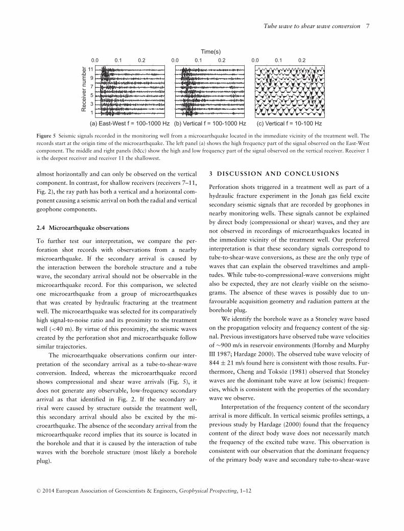
Figure 5 Seismic signals recorded in the monitoring well from a microearthquake located in the immediate vicinity of the treatment well. Therecords start at the origin time of the microearthquake. The left panel (a) shows the high frequency part of the signal observed on the East-Westcomponent. The middle and right panels (b&c) show the high and low frequency part of the signal observed on the vertical receiver. Receiver 1is the deepest receiver and receiver 11 the shallowest.

almost horizontally and can only be observed on the verticalcomponent. In contrast, for shallow receivers (receivers 7–11,Fig. 2), the ray path has both a vertical and a horizontal com-ponent causing a seismic arrival on both the radial and verticalgeophone components.

2.4 Microearthquake observations

To further test our interpretation, we compare the per-foration shot records with observations from a nearbymicroearthquake. If the secondary arrival is caused bythe interaction between the borehole structure and a tubewave, the secondary arrival should not be observable in themicroearthquake record. For this comparison, we selectedone microearthquake from a group of microearthquakesthat was created by hydraulic fracturing at the treatmentwell. The microearthquake was selected for its comparativelyhigh signal-to-noise ratio and its proximity to the treatmentwell (<40 m). By virtue of this proximity, the seismic wavescreated by the perforation shot and microearthquake followsimilar trajectories.

The microearthquake observations confirm our inter-pretation of the secondary arrival as a tube-to-shear-waveconversion. Indeed, whereas the microearthquake recordshows compressional and shear wave arrivals (Fig. 5), itdoes not generate any observable, low-frequency secondaryarrival as that identified in Fig. 2. If the secondary ar-rival were caused by structure outside the treatment well,this secondary arrival should also be excited by the mi-croearthquake. The absence of the secondary arrival from themicroearthquake record implies that its source is located inthe borehole and that it is caused by the interaction of tubewaves with the borehole structure (most likely a boreholeplug).

3 D ISCUSS ION AND C ONCLUSIONS

Perforation shots triggered in a treatment well as part of ahydraulic fracture experiment in the Jonah gas field excitesecondary seismic signals that are recorded by geophones innearby monitoring wells. These signals cannot be explainedby direct body (compressional or shear) waves, and they arenot observed in recordings of microearthquakes located inthe immediate vicinity of the treatment well. Our preferredinterpretation is that these secondary signals correspond totube-to-shear-wave conversions, as these are the only type ofwaves that can explain the observed traveltimes and ampli-tudes. While tube-to-compressional-wave conversions mightalso be expected, they are not clearly visible on the seismo-grams. The absence of these waves is possibly due to un-favourable acquisition geometry and radiation pattern at theborehole plug.

We identify the borehole wave as a Stoneley wave basedon the propagation velocity and frequency content of the sig-nal. Previous investigators have observed tube wave velocitiesof ∼900 m/s in reservoir environments (Hornby and MurphyIII 1987; Hardage 2000). The observed tube wave velocity of844 ± 21 m/s found here is consistent with those results. Fur-thermore, Cheng and Toksoz (1981) observed that Stoneleywaves are the dominant tube wave at low (seismic) frequen-cies, which is consistent with the properties of the secondarywave we observe.

Interpretation of the frequency content of the secondaryarrival is more difficult. In vertical seismic profiles settings, aprevious study by Hardage (2000) found that the frequencycontent of the direct body wave does not necessarily matchthe frequency of the excited tube wave. This observation isconsistent with our observation that the dominant frequencyof the primary body wave and secondary tube-to-shear-wave



0 0.1Time (s)

1

23

4

5

6

P

0 0.1

600

560

520

Dep

th (m

)

Time (s)

1

23

4

5

6

P

0 0.1Time (s)

1

23

4

5

6

P

0 0.1

600

560

520D

epth

(m)

Time (s)

1

23

4

5

6

P

(a)

(d)(c)

(b)

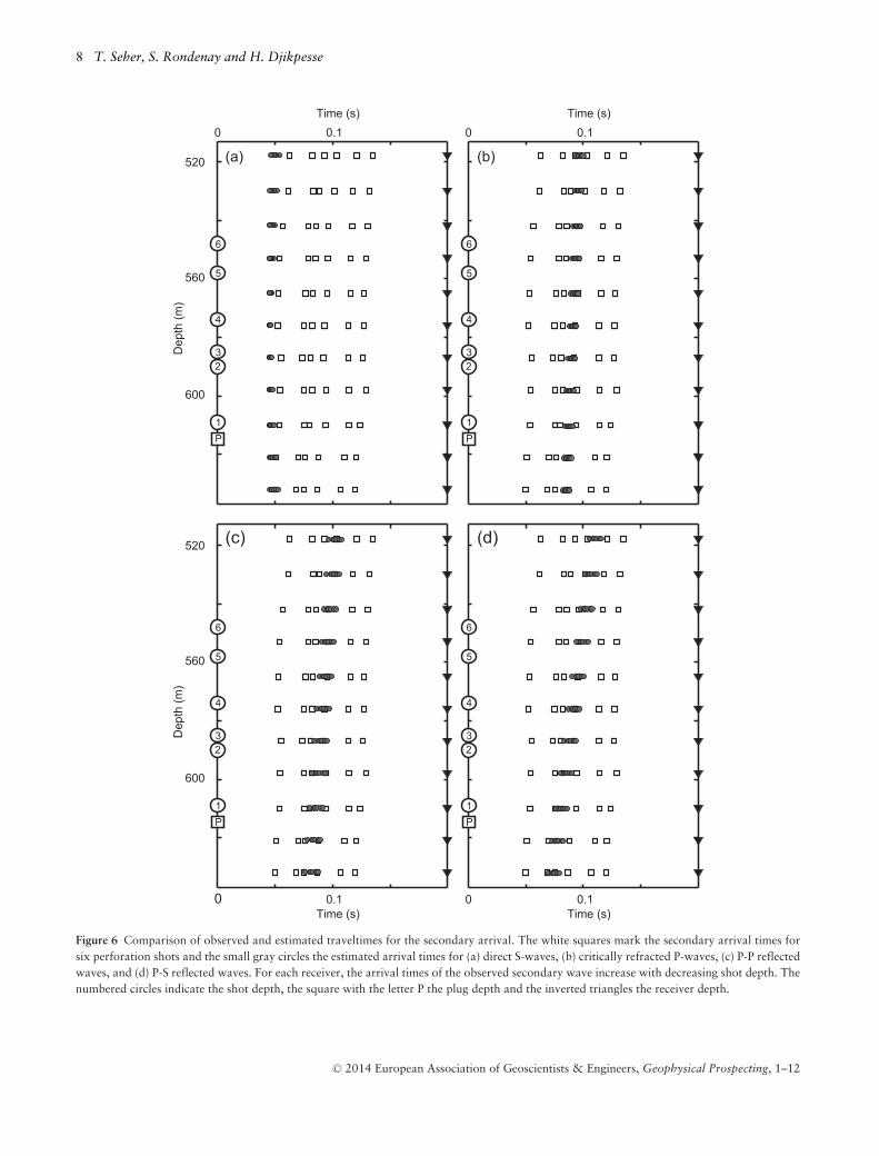
Figure 6 Comparison of observed and estimated traveltimes for the secondary arrival. The white squares mark the secondary arrival times forsix perforation shots and the small gray circles the estimated arrival times for (a) direct S-waves, (b) critically refracted P-waves, (c) P-P reflectedwaves, and (d) P-S reflected waves. For each receiver, the arrival times of the observed secondary wave increase with decreasing shot depth. Thenumbered circles indicate the shot depth, the square with the letter P the plug depth and the inverted triangles the receiver depth.



conversion differ by an order of magnitude. However, thisdifference implies that either the perforation shot excites bothhigh frequency body waves and low frequency tube waves, orthat tube-to-shear-wave conversion leads to an amplificationof low frequencies.

While tube-to-body-wave conversions at discontinuitieshave been observed before (White and Sengbush 1963;Lee et al. 1984), these converted waves have not been system-atically explored in the context of hydraulic fracture experi-ments. The correct identification of these waves is particularlyimportant, because tube-to-shear-wave conversions may eas-ily be confused with direct shear wave arrivals. A distinctionbetween the two is particularly difficult if only a single per-foration shot is analyzed. In this study, for example, a directshear wave would arrive at a similar time as the tube-to-shear-wave conversion generated by the deepest perforationshot (Fig. 6a in the appendix).

Once identified, the converted waves allow the direct, in-dependent measurement of both the tube wave velocity andthe formation’s shear wave velocity. The tube wave veloc-ity can be estimated from the traveltime difference betweentwo successive perforation shots, provided that the locationand time of the perforation shots are known. The forma-tion’s shear wave velocity can be calculated based on themoveout of the secondary arrivals across the receiver arrayfor a single perforation shot. This estimate is independentof origin time and tube wave velocity. The latter estimate isparticularly useful if the perforation shot did not create ob-servable direct shear waves.

The converted waves identified in this study can helpfine-tune the experimental parameters in hydraulic fracturingoperations. Better controls on the perforation shots (locationand origin time) and the receivers (location, orientation andcoupling) yield an improved calibration of the velocity model.This, in turn, allows for a more precise location of inducedmicroseismicity and thereby an improved steering of the hy-draulic fracture process. More robust velocity models (includ-ing anisotropy) may also help better characterize the fracturedirection and stress field in the reservoir.

The observations presented here also have important im-plications for subsurface velocity estimation and imaging,as they yield improved illumination and increased frequencycontent. With regards to illumination, the tube-to-body-waveconversions improve the ray coverage because the plug actsas a secondary seismic source that emits waves with differentray paths than those generated by the primary source. Thismay significantly improve the illumination in obscured partsof the model. With regards to frequency content, it has been

shown that the quality of a seismic model is linked to thespectral bandwidth of the available seismic data. For exam-ple, Wu and Toksoz (1987) demonstrated that using multiplefrequencies improves the image quality in seismic diffractiontomography. Similarly, using low seismic frequencies helps toconstrain the long wavelength velocity structure in full wave-form inversion (Sirgue and Pratt 2004; Virieux and Operto2009). However, the spectral bandwidth afforded by activeseismic sources is usually limited. In this study, the primaryenergy of the perforation shots is above 100 Hz while theenergy of the secondary arrival is below 100 Hz. Since thefrequency contents of the primary and secondary arrivals dif-fer, the secondary arrivals effectively widen the spectrum ofavailable seismic energy and may thus improve the resolutionachieved by the recorded seismic waveforms. Integration ofthe secondary arrivals may therefore help to derive a seismicmodel or image that is superior to the one derived from pri-mary (direct) arrivals alone.

Finally, our indirect measurements of low-frequencyStoneley wave velocity in the treatment well, in combinationwith sonic log measurements made at high frequency, mayprovide a new way to assess velocity dispersion – a propertydirectly related to seismic attenuation. Stoneley waves havebeen shown to be dispersive in borehole settings. For exam-ple, Stewart et al. (1984) demonstrated that velocity measure-ments at sonic and seismic frequencies give significantly dif-ferent results due to velocity dispersion. Winkler et al. (1989)also documented a frequency dependence of Stoneley wavevelocities in boreholes. However, to exploit this property forsubsurface characterization purposes, one needs to observelow-frequency Stoneley waves. In ideal conditions the tube-to-shear-wave signals identified in this study allow such an ob-servation, and as such they provide a novel means of assessingseismic attenuation near the borehole. This new insight intoattenuation, in turn, may yield improved constraints on frac-ture density, porosity and permeability in the vicinity of thewell, which are key parameters for reservoir characterization.

ACKNOWLEDGEMENTS

This work was made possible by funding from MIT’s EarthResources Laboratory and Schlumberger-Doll Research. Wewould like to thank Julie Shemeta and Nancy House for shar-ing results and giving us access to Encana’s seismic data.We greatly profited from discussions with Mark Willis andElizabeth LaBarre. We are thankful to two anonymous re-viewers and the associate editor, whose advice helped improveour original manuscript.



REFERENCES

Aki K. and Richards P.G. 2002. Quantitative Seismology. UniversityScience Books, 2nd edition.

Albright J.N. and Johnson P.A. 1990. Cross-borehole observation ofmode conversion from borehole Stoneley waves to channel wavesat a coal layer. Geophysical Prospecting 38(6), 607–620.

Aldridge D.F. 1992. Comments on “Conversion points and trav-eltimes of converted waves in parallel dipping layers” by GisaTessmer and Alfred Behle. Geophysical Prospecting 40(1), 101–103.

Aronstam P.S. 2004. Use of minor borehole obstructions as seismicsources. US Patent 6, 747, 914.

Beydoun W.B., Cheng C.H. and Toksoz M.N. 1985. Detection ofopen fractures with vertical seismic profiling. Journal of Geophys-ical Research 90(B6), 4557–4566.

Cheng C.H. and Toksoz M.N. 1981. Elastic wave propagation in afluid-filled borehole and synthetic acoustic logs. Geophysics 46(7),1042–1053.

Greenhalgh S., Zhou B. and Cao S. 2003. A crosswell seismic ex-periment for nickel sulphide exploration. Journal of Applied Geo-physics 53( 2–3), 77–89.

Greenhalgh S.A., Mason I.M. and Sinadinovski C. 2000. In-mine seis-mic delineation of mineralization and rock structure. Geophysics65(6), 1908–1919.

Hardage B.A. 2000. Vertical Seismic Profiling: Principles, vol. 14,Handbook of Geophysical Exploration Seismic Exploration. Perg-amon Press, 3rd edition.

Hornby B.E. and Murphy III W.F. 1987. Vp/Vs in unconsoli-dated oil sands: Shear from Stoneley. Geophysics 52(4), 502–513.

Kwan A., Dudley J. and Lantz E. 2002. Who really discovered Snell’slaw? Physics World 15(4), 64.

Lee M.W., Balch A.H. and Parrott K.R. 1984. Radiation from adownhole air gun source. Geophysics 49(1), 27–36.

Maxwell S.C., Shemeta J. and House N. 2006. Integrated anisotropicvelocity modeling using perforation shots, passive seismic and vspdata. 68th EAGE Conference & Exhibition, Extended Abstracts,A046.

Norris M. and Aronstam P. 2003. Use of autonomous moveable ob-structions as seismic sources. US Patent 6,662,899.

Robinson J.W. and Shanley K.W. (ed.). 2005. Jonah Field: Case Studyof a Tight-Gas Fluvial Reservoir, Vol. 52. AAPG Studies in Ge-ology, American Association of Petroleum Geologists and RockyMountain Association of Geologists.

Seher T., Rondenay S. and Djikpesse H. 2011. Hydraulic FractureMonitoring: A Jonah Field Case Study. Earth Resources LaboratoryConsortium Meeting.

Sirgue L. and Pratt R.G. 2004. Efficient waveform inversion andimaging: A strategy for selecting temporal frequencies. Geophysics69(1), 231–248.

Stewart R.R., Huddleston P.D. and Kan T.K. 1984. Seismic ver-sus sonic velocities: A vertical seismic profiling study. Geophysics49(8), 1153–1168.

Taylor G.G. 1989. The point of p-s mode-converted reflection: Anexact determination. Geophysics 54(8), 1060–1063.

Tessmer G. and Behle A. 1988. Common reflection point data-stacking technique for converted waves. Geophysical Prospecting36(7), 671–688.

Tessmer G., Krajewski P., Fertig J. and Behle A. 1990. Processing ofPS-reflection data applying a common conversion-point stackingtechnique. Geophysical Prospecting 38(3), 267–268.

Virieux J. and Operto S. 2009. An overview of full-waveform inver-sion in exploration geophysics. Geophysics 74(6), WCC1–WCC26.

White J.E. and Sengbush R.L. 1963. Shear waves from explosivesources. Geophysics 28(6), 1001–1019.

Wills P.B., DeMartini D.C., Vinegar H.J., Shlyapobersky J., DeegW.F., Woerpel J.C., Fix J.E., Sorrelis G.G. and Adair R.G. 1992.Active and passive imaging of hydraulic fractures. Leading Edge11(7), 15–22.

Winkler K.W., Liu H.-L. and Johnson D.L. 1989. Permeability andborehole Stoneley waves: Comparison between experiment and the-ory. Geophysics 54(1), 66–75.

Wu R.S. and Toksoz M.N. 1987. Diffraction tomography and mul-tisource holography applied to seismic imaging. Geophysics 52(1),11–25.

Xu K. and Greenhalgh S. 2010. Ore-body imaging by crosswell seis-mic waveform inversion: A case study from Kambalda, WesternAustralia. Journal of Applied Geophysics 70(1), 38–45.

APPENDIX A

Origin time and event location

The origin time of perforation shots and the origin time andlocation of microseismic events is generally not well known inhydraulic fracturing experiments. When appropriate measure-ment devices are used, the firing time of perforation shots canbe accurately detected through electrical signals that sense thedetonator firing. Otherwise, this origin time problem needsto be addressed during data processing. For single receiverwells, a standard workflow usually includes the followingprocessing steps. (1) Waveform data corresponding to theperforation shots are extracted, and used to estimate P-waveand S-wave traveltimes and azimuths. (2) An initial velocitymodel is derived from well log measurements. (3) The veloc-ity model is updated using the perforation shot traveltimesto account for possible lateral variations. This only requiresknowledge of the source and receiver location and allows usto calibrate the origin time of the perforation shot and esti-mate both P-wave and S-wave velocities. (4) The perforationshot data are used to orient the receivers into a North-South/East-West reference frame. (5) The waveform data corre-sponding to microearthquakes are extracted and rotated intoa North-South / East-West reference frame. P-wave and S-wave traveltimes and azimuths are measured for the mi-croearthquakes. (6) The microearthquakes are relocated using



both traveltime and azimuth data. A more complete descrip-tion of this workflow and its application to the data from theJonah field are presented in Seher et al. (2011).

APPENDIX B

Traveltimes of direct, reflected and critically refracted waves

The first observation we use to identify the secondary arrivalis the traveltime difference between successive shots observedat one receiver (Fig. 2). The variable shot depth is the mostlikely cause for the traveltime differences, since the explosivesperforated the borehole at different depths and all other ex-periment parameters remained unchanged. To test whetherdifferent seismic waves can explain the observed traveltimedifference, we calculate traveltimes for direct shear waves, re-flections at the base of the formation (PP, PS, SP, or SS), andcritical refractions at the base of the formation.

In this study we derive analytic traveltimes for reflectionsand refractions in a constant velocity medium from Snell’s law(Kwan et al. 2002). First, we estimate traveltimes for directshear waves:

Ts = β−11

√d2 + (hs − hr )2 , (B1)

where d stands for the horizontal source receiver spacing, hs

and hr represent the depth of the source and receiver abovethe interface, and β1 denotes the average shear wave velocityof the formation. The traveltime fit is shown in Figure 6a.

Second, we derive analytic traveltimes Tc for criticallyrefracted P waves:

Tc = α−11 (hs + hr ) cos λc + α−1

2 d , (B2)

where α1 and α2 denote the velocity in the upper and lowermedium, respectively, and λc is the critical angle defined bythose velocities. To find the depth of the interface and velocityof the lower layer, we minimize the root mean square misfitbetween the calculated and observed traveltimes using gridsearch. The best traveltime fit is shown in Fig. 6b.

Third, we estimate analytic traveltimes Tpp for compres-sional wave reflections:

Tpp = α−11

√d2 + (hs + hr )2 . (B3)

We again search the interface depth that provides thesmallest root mean square misfit between the observationsand the calculated traveltimes. More details can be found inAki and Richards (2002).

Finally, we evaluate the traveltimes Tps for PS reflections.The traveltimes can be found analytically by solving a quarticequation for the conversion point (Tessmer and Behle 1988;

Taylor 1989; Tessmer et al. 1990; Aldridge 1992). Instead weevaluate:

Tps = α−11 hs sec λα + β−1

1 hr sec λβ , (B4)

where λα and λβ represent the angles of incidence and re-flection of the P- and S-waves, respectively. The angles canbe determined from the horizontal slowness p = α−1

1 sin λα =β−1

1 sin λβ by solving the equation:

hsαp√1 − α2 p2

+ hrβp√1 − β2 p2

= d (B5)

for the horizontal slowness p. Again, the smallest traveltimemisfit is found by varying the depth of the reflecting interface(Fig. 6d). Note that in this analysis we did not consider SS andSP reflections because no direct S waves are observed in therecorded signal.

Each seismic wave can explain some of the observed trav-eltimes, but none of them explains systematically all the ob-served traveltimes. In particular, the estimated traveltime dif-ferences for any pair of successive shots are always smallerthan the observed traveltime differences. Thus, we concludethat direct shear waves and waves reflected/refracted at abounding horizontal interface do not fit the observed trav-eltimes. We remark, however, that this analysis demonstratesthe need for multiple seismic sources to facilitate the identifi-cation of the secondary arrival.

A similar exercise was conducted for reflec-tions/refractions at the top of the formation, but wefound that these wave interactions could not explain thesecondary arrival either because they produce the wrongmoveout (i.e., the seismic waves arrive earlier at the top thanat the bottom of the monitoring well, which is the oppositeof what we observe).

APPENDIX C

Traveltimes of conical waves and tube waves

The second observation we use to identify the secondary arrivalis the traveltime variation for a single shot observed at differ-ent receivers (Fig. 2). For the remote observation of conicalwaves propagating in the treatment well, the total traveltimedepends on the traveltime Tt of the wave along the well andthe traveltime Tm from the treatment to the monitoring well.The total traveltime T is

T ≈ Tt + Tm . (C1)

If the velocity is approximately constant and the twowells are parallel, the traveltime Tm between the treatment



and monitoring well is approximately equal for all receivers.The traveltime difference observed on two receivers is thenequal to

�T ≈ �Tt ≈ �l/v . (C2)

This difference depends on the velocity v inside the treat-ment well and the path length l along the well. Because the twowells are approximately parallel, this length is approximatelyequal to the receiver spacing.

This relationship allows us to rule out conical waves inthe measurement well as an explanation for the observed

secondary arrivals. In this study, we observe a traveltimedifference of ∼15 ms across the receiver array (Fig. 2).With a receiver array length of 114 m, this would im-ply a tube wave velocity of ∼7.6 km/s – a velocity that ismuch too high for fluid filled boreholes or the surroundingreservoir.

We note that the same argument rules out a diffraction atthe bottom of the monitoring well and the remote observationof tube waves in the treatment well as explanations for thesecondary arrival (i.e., both would imply an unrealisticallyhigh velocity along the well axis).


tube wave to shear wave conversion at borehole...

Documents