The International Workshop on Applied Modeling and Simulation, 2019 978-88-85741-44-7; Bruzzone, Longo, Solis Eds I

TTHHEE 1122TTHH

IINNTTEERRNNAATTIIOONNAALL WWOORRKKSSHHOOPP OONN

AAPPPPLLIIEEDD MMOODDEELLIINNGG && SSIIMMUULLAATTIIOONN

OCTOBER 30 - 31 2019

NUSS KENT RIDGE GUILD HOUSE SINGAPORE

EDITED BY AGOSTINO G. BRUZZONE

FRANCESCO LONGO ADRIANO SOLIS

PRINTED IN RENDE (CS), ITALY, SEPTEMBER 2019

Volume ISBN 978-88-85741-43-0 (paperback) Volume ISBN 978-88-85741-44-7 (PDF)

Proceedings of WAMS, ISBN 978-88-85741-43-0 (paperback)

Proceedings of WAMS, ISBN 978-88-85741-44-7 (PDF)

The International Workshop on Applied Modeling and Simulation, 2019 978-88-85741-44-7; Bruzzone, Longo, Solis Eds II

2019 DIME UNIVERSITÀ DI GENOVA, DIMEG UNIVERSITY OF CALABRIA

RESPONSIBILITY FOR THE ACCURACY OF ALL STATEMENTS IN EACH PAPER RESTS SOLELY WITH THE AUTHOR(S). STATEMENTS

ARE NOT NECESSARILY REPRESENTATIVE OF NOR ENDORSED BY THE DIME, UNIVERSITY OF GENOA OR DIMEG UNIVERSITY

OF CALABRIA. PERMISSION IS GRANTED TO PHOTOCOPY PORTIONS OF THE PUBLICATION FOR PERSONAL USE AND FOR THE

USE OF STUDENTS PROVIDING CREDIT IS GIVEN TO THE CONFERENCES AND PUBLICATION. PERMISSION DOES NOT EXTEND TO

OTHER TYPES OF REPRODUCTION NOR TO COPYING FOR INCORPORATION INTO COMMERCIAL ADVERTISING NOR FOR ANY

OTHER PROFIT – MAKING PURPOSE. OTHER PUBLICATIONS ARE ENCOURAGED TO INCLUDE 300 TO 500 WORD ABSTRACTS OR

EXCERPTS FROM ANY PAPER CONTAINED IN THIS BOOK, PROVIDED CREDITS ARE GIVEN TO THE AUTHOR(S) AND THE

CONFERENCE. FOR PERMISSION TO PUBLISH A COMPLETE PAPER WRITE TO: DIME UNIVERSITY OF GENOA, PROF. AGOSTINO G. BRUZZONE, VIA OPERA PIA 15, 16145 GENOVA, ITALY OR TO DIMEG UNIVERSITY OF CALABRIA, PROF. FRANCESCO

LONGO, VIA P.BUCCI 45C, 87036 RENDE, ITALY. ADDITIONAL COPIES OF THE PROCEEDINGS OF THE EMSS ARE AVAILABLE

FROM DIME UNIVERSITY OF GENOA, PROF. AGOSTINO G. BRUZZONE, VIA OPERA PIA 15, 16145 GENOVA, ITALY OR

FROM DIMEG UNIVERSITY OF CALABRIA, PROF. FRANCESCO LONGO, VIA P.BUCCI 45C, 87036 RENDE, ITALY

Volume ISBN 978-88-85741-43-0 (paperback) Volume ISBN 978-88-85741-44-7 (PDF) Proceedings of WAMS, ISBN 978-88-85741-43-0 (paperback) Proceedings of WAMS, ISBN 978-88-85741-44-7 (PDF)

The International Workshop on Applied Modeling and Simulation, 2019 978-88-85741-44-7; Bruzzone, Longo, Solis Eds III

THE 12TH INTERNATIONAL WORKSHOP ON

APPLIED MODELLING AND SIMULATION

OCTOBER 30 - 31 2019 SINGAPORE

ORGANIZED BY

SIMULATION TEAM

DIME – UNIVERSITY OF GENOA

IMCS – INTERNATIONAL MULTIDISCIPLINARY COUNCIL OF SIMULATION

MSC-LES, MODELING & SIMULATION CENTER, LABORATORY OF ENTERPRISE

SOLUTIONS

MCLEOD INSTITUTE OF TECHNOLOGY AND INTEROPERABLE MODELING AND

SIMULATION – GENOA CENTER

LATVIAN SIMULATION CENTER

SPANISH SIMULATION CENTER - LOGISIM

LSIS – LABORATOIRE DES SCIENCES DE L’INFORMATION ET DES SYSTEMES, MARSEILLE

PERUGIA SIMULATION CENTER

LIOPHANT SIMULATION

MCLEOD INSTITUTE OF TECHNOLOGY AND INTEROPERABLE MODELING &

SIMULATION, SIMULATION TEAM, GENOA CENTER

M&SNET

LATVIAN SIMULATION SOCIETY

MIK, RIGA TU

The International Workshop on Applied Modeling and Simulation, 2019 978-88-85741-44-7; Bruzzone, Longo, Solis Eds IV

GRVA LAMCE COPPE UFRJ

RUSSIAN SIMULATION SOCIETY

FCEIA, UNIVERSIDAD NACIONAL DE ROSARIO

NATO M&S CENTRE OF EXCELLENCE

MIMOS – MOVIMENTO ITALIANO MODELLAZIONE E SIMULAZIONE

CENTRAL LABS

UNIVERSITY OF CAGLIARI

ASIASIM

NATIONAL UNIVERSITY OF SINGAPORE

NANYANG TECHNOLOGICAL UNIVERSITY

SOCIETY OF SIMULATION AND GAMING OF SINGAPORE

WAMS2019 INDUSTRIAL SPONSOR

CAL-TEK SRL

LIOTECH LTD

MAST SRL

SIM-4-FUTURE

WAMS 2019 MEDIA PARTNER

The International Workshop on Applied Modeling and Simulation, 2019 978-88-85741-44-7; Bruzzone, Longo, Solis Eds V

EDITORS AGOSTINO BRUZZONE SIMULATION TEAM GENOA, UNIVERSITY OF GENOA, ITALY agostino@itim.unige.it

FRANCESCO LONGO MSC-LES, UNIVERSITY OF CALABRIA, ITALY f.longo@unical.it

ADRIANO SOLIS YORK UNIVERSITY, CANADA asolis@yorku.ca

The International Workshop on Applied Modeling and Simulation, 2019 978-88-85741-44-7; Bruzzone, Longo, Solis Eds VI

THE 12TH INTERNATIONAL WORKSHOP ON

APPLIED MODELLING AND SIMULATION, WAMS 2019

GENERAL CHAIR AGOSTINO BRUZZONE, SIMULATION TEAM GENOA, UNIVERSITY OF GENOA, ITALY

PROGRAM CO-CHAIRS FRANCESCO LONGO, MSC-LES, UNIVERSITY OF CALABRIA ITALY ADRIANO SOLIS, YORK UNIVERSITY, CANADA

ORGANIZATION CO-CHAIRS MARINA MASSEI, DIME UNIVERSITY OF GENOA, ITALY LUCA BUCCHIANICA, GEA SINGAPORE, SINGAPORE CECILIA ZANNI-MERK, ICUBE, INSA STRASBOURG, FRANCE

The International Workshop on Applied Modeling and Simulation, 2019 978-88-85741-44-7; Bruzzone, Longo, Solis Eds VIII

WAMS 2019 STEERING COMMITTEE AGOSTINO BRUZZONE, STRATEGOS, UNIVERSITY OF GENOA, ITALY FELIX BREITENECKER, WIEN TU, AUSTRIA ROBERTO CIANCI, DIME, ITALY MICHAEL CONROY, KSC NASA, USA LUCIANO DI DONATO, INAIL, ITALY GERSON GOMES CUNHA, COPPE UFRJ, BRAZIL RICCARDO DI MATTEO, SIMULATION TEAM, SIM4FUTURE, ITALY PAOLO FADDA, CENTRAL LABS, ITALY GIANFRANCO FANCELLO, UNIVERSITY OF CAGLIARI, ITALY MARCO FRASCIO, UNIGE, ITALY CLAUDIA FRYDMAN, LSIS, FRANCE MURAT GUNAL, TURKISH NAVAL ACADEMY, TURKEY JEN HSIEN HSU, DE MONTFORRT UNIVERSITY, LEEDS, UK JANOS SEBESTYEN JANOSY, CENTRE FOR ENERGY RESEARCH, HUNGARIAN

ACADEMY OF SCIENCES, HUNGARY EMILIO JIMÉNEZ, UNIVERSIDAD DE LA RIOJA, SPAIN ALI RIZA KAYLAN, BOGAZICI UNIVERSITY, TURKEY LUIZ LANDAU, LAMCE UFRJ, BRAZIL FRANCESCO LONGO, UNICAL, ITALY MARINA MASSEI, LIOPHANT,ITALY MATTEO AGRESTA, DIME, ITALY IAN MAZAL, BRNO UNIVERSITY OF DEFENCE, CZECH UNIVERSITY YURI MERKURYEV, RIGA TU, LATVIA TUNCER OREN, OTTAWA INTERNATIONAL, CANADA MIQUEL ANGEL PIERA, SPAIN/BARCELONA , SPAIN ANDREA REVERBERI, DCCI, ITALY STEFANO SAETTA, UNIVERSITY OF PERUGIA, ITALY ROBERTA SBURLATI, DICCA, ITALY KIRIL SINELSHCHIKOV, SIM4FUTURE ADRIANO SOLIS, YORK UNIVERSITY, CANADA GRAZIA TUCCI, DICEA, FLORENCE UNIVERSITY, ITALY GREGORY ZACHAREWICZ, IMS UNIVERSITY OF BORDEAUX, FRANCE CECILIA ZANNI-MERK, ICUBE, INSA STRASBOURG, FRANCE

WAMS 2019 LOCATION NUSS, KENT RIDGE GUILD HOUSE 9 KENT RIDGE DRIVE, 119241, SINGAPORE

WAMS 2019 SCIENTIFIC & SOCIAL EVENTS WEDNESDAY, OCTOBER 30TH OCT 30, 845-1200 ASIASIM & WAMS OPENING, KEYNOTE SPEECHES

OCT.30, 1200-1330 ASIASIM & WAMS WORKING LUNCH

OCT.30, 1400-1730 STRATEGOS WORKSHOP

OCT.30, 1800-1930 ASIASIM & WAMS WELCOME COCKTAIL

OCT.30, 2100-2230 WAMS NIGHT DRINK AT LONG BAR, RAFFLES HOTEL

THURSDAY, OCTOBER 31ST OCT.31, 900-1200 WAMS SESSION 1 & 2

OCT.31, 1200-1330 ASIASIM & WAMS WORKING LUNCH

OCT.31, 900-1200 WAMS SESSION 3 & 4

OCT.31, 1900-2200 GALA DINNER AT S.E.A. AQUARIUM IF YOU ARE INTERESTED YOU CAN ALSO SEND REQUEST TO FREE

PARTICIPATION TO:

FRIDAY, NOVEMBER 1ST NOV.1, 1400-1700 JAMES COOK & GENOA UNIVERSITY WORKSHOP (OPTIONAL)

TRACKS AND WORKSHOP CHAIRS DIGITAL FRUITION OF CULTURAL HERITAGE & ARCHITECTURE CHAIRS: GRAZIA TUCCI, FLORENCE UNIVERSITY SERIOUS GAMES CHAIRS: MICHAEL CONROY, KSC NASA, RICCARDO DI MATTEO, MAST

SIMULATION TECHNIQUES AND METHODOLOGIES CHAIRS: GIOVANNI LUCA MAGLIONE, SIM4FUTURE; SIMONE

YOUNGBLOOD, APL JOHNS HOPKINGS UNIVERSITY, USA

SIMULATION FOR APPLICATIONS CHAIRS: MATTEO AGRESTA, UNIVERSITY OF GENOA; JEN HSIEN

HSU, DE MONTFORRT UNIVERSITY, LEEDS, UK

SIMULATION FOR EMERGENCY & CRISIS MANAGEMENT CHAIRS: MARINA MASSEI, DIME, ITALY - TERRY BOSSOMAIER, CHARLES STURT UNIVERSITY, AUSTRALIA

SIMULATION TOOLS FOR HUMAN RELIABILITY ANALYSIS STUDIES CHAIR: ANTONELLA PETRILLO, UNIVERSITY OF NAPOLI, PARTENOPE, ITALY

SERIOUS GAMES FOR STRATEGY CHAIRS: FRANCESCO BELLOTTI, ELIOS LAB, ITALY - GREGORY

ZACHAREWICZ,UNIVERSITY OF BORDEAUX

STRATEGIC ENGINEERING & SIMULATION CHAIRS: AGOSTINO BRUZZONE, SIMULATION TEAM GENOA, UNIVERSITY OF GENOA, ITALY - IAN MAZAL, BRNO UNIVERSITY

OF DEFENCE, CZECH REP. - ANNA FRANCA SCIOMACHEN, DIEC, ITALY

CBRN & CRISIS SIMULATION CHAIRS: ANDREA REVERBERI, DCCI, ITALY

IMMERSIVE SOLUTION FOR PRODUCT DESIGN CHAIRS: LETIZIA NICOLETTI, CAL-TEK SRL

INNOVATIVE SOLUTIONS SUPPORTING INTEROPERABILITY

STANDARDS CHAIRS: ANTONIO PADOVANO, MSC-LES, UNICAL MIXED REALITY & MOBILE TRAINING ENABLING NEW

EDUCATIONAL SOLUTION CHAIR: MARCO VETRANO, SIMULATION TEAM

The International Workshop on Applied Modeling and Simulation, 2019 978-88-85741-44-7; Bruzzone, Longo, Solis Eds IX

WAMS CO-CHAIRS’ MESSAGE:

WELCOME TO WAMS 2019!

DEAR PARTICIPANTS, THIS YEAR WE MOVE TO SINGAPORE FOR THE 12TH EDITION

OF WAMS, AFTER EUROPE AND AMERICA WE ARE EXPLORING ALSO ASIAS, THEREFORE THE EVENT HAD SINCE ITS BEGINNING REGISTERED PARTICIPATION

FROM ALL AROUND THE WORLD. THIS SINGAPORE EDITION IS DEVELOPED IN STRONG SYNERGY WITH OUR

COLLEAGUES OF ASIASIM, NATIONAL UNIVERSITY OF SINGAPORE, NANYANG

TECHNOLOGICAL UNIVERSITY AND THE SOCIETY OF SIMULATION AND GAMING OF

SINGAPORE. INDEED 2019 EDITION IS CO-LOCATED WITH ASIASIM 2019 INTO

THE WONDERFUL STRUCTURE OF THE NUSS AT KENT RIDGE GUILD HOUSE. WAMS IS ALSO HOSTING THE STRATEGOS WORKSHOP: A NEW WAY TO

SUCCEED DEVOTED TO PRESENT THE INNOVATIVE CONCEPT OF STRATEGIC

ENGINEERING COMBINING MODELLING, SIMULATION, AI AND DATA ANALYTICS

TO SUPPORT STRATEGIC DECISION MAKING. THIS YEAR, AS ALWAYS, WE APPLIED A QUALIFIED PEER REVIEW TO GUARANTEE

HIGH QUALITY OF THE PAPERS TO COMPLETE A VALID SELECTION THAT OPENS

ACCESS TO SEVERAL INTERNATIONAL JOURNALS CONNECTED TO I3M & WAMS: THERE ARE 9 JOURNALS READY TO EVALUATE OUR PAPER EXTENSIONS. WAMS IN SINGAPORE REPRESENTS AN UNIQUE OPPORTUNITY TO GET IN TOUCH

WITH A WIDE COMMUNITY OF SCIENTISTS, TECHNICIANS, MANAGERS FROM

INSTITUTIONS, COMPANIES AND GOVERNMENTAL ORGANIZATIONS INTERESTED IN

APPLYING MODELING & SIMULATION IN MANY DIFFERENT SECTORS FROM

SHIPPING TO INDUSTRY, FROM HOMELAND SECURITY TO BUSINESS, SO WE

ENCOURAGE YOU TO ATTEND THE SESSIONS AND WORKSHOPS AS WELL AS TO

ENJOY THE BEAUTIFUL SOCIAL EVENTS SUCH AS THE GALA DINNER AT S.E.A. AQUARIUM, THE ASIASIM & WAMS WELCOME COCKTAIL AT NUSS AND THE WAMS NIGHT DRINK AT LONG BAR IN RAFFLES HOTEL. NEXT YEAR THE EVENT WILL BE BACK IN EUROPE, THEREFORE WE ARE WORKING

ON REINFORCING CONNECTIONS WITH AMERICA AND ASIA AND WE WELCOME AS

ALWAYS PROPOSALS FOR NEW TRACKS AND NEW EVENTS FROM SCIENTISTS AND

EXPERTS FROM ALL AROUND THE WORLD.

AGOSTINO G. BRUZZONE FRANCESCO LONGO ADRANO SOLIS MARINA MASSEI

The International Workshop on Applied Modeling and Simulation, 2019 978-88-85741-44-7; Bruzzone, Longo, Solis Eds X

ACKNOWLEDGEMENTS

The WAMS 2019 International Program Committee (IPC) has selected the papers for the Conference among many submissions; therefore, based on this effort, a very successful event is expected. The WAMS 2019 IPC would like to thank all the authors as well as the reviewers for their invaluable work. A special thank goes to all the organizations, institutions and societies that have supported and technically sponsored the event.

WAMS 2019 INTERNAL STAFF AGOSTINO G. BRUZZONE, DIME, UNIVERSITY OF GENOA, ITALY MATTEO AGRESTA, SIMULATION TEAM ALESSANDRO CHIURCO, CAL-TEK SRL, ITALY RICCARDO DI MATTEO, SIMULATION TEAM, ITALY CATERINA FUSTO, DIMEG, UNIVERSITY OF CALABRIA, ITALY FRANCESCO LONGO, MSC-LES, ITALY MARINA MASSEI, LIOPHANT SIMULATION LETIZIA NICOLETTI, CAL-TEK SRL ANTONIO PADOVANO, DIMEG, UNIVERSITY OF CALABRIA, ITALY KIRIL SINELSHCHIKOV, SIM4FUTURE MARCO VETRANO, CAL-TEK SRL, ITALY LORENZO VOLPE, LIOPHANT SIMULATION

WAMS SOCIAL EVENTS & Venues in Singapore & Social Events:

AsiaSim, WAMS & STRATEGOS & Welcome Cocktail (Included) @ NUSS Kent Ridge Guild House, National University of Singapore, 9 Kent Ridge Drive

STRATEGOS & WAMS Night Drink (No Host ) @ Long Bar, Raffles Hotel, Raffles Arcade, 328 North Bridge Rd,

AsiaSim & WAMS Gala Dinner (Included) @S.E.A. Aquarium, Resorts World Sentosa, 8 Sentosa Gateway, Sentosa Island

IN ADDITION WAMS ATTENDEES ARE INVITED TO THE ASIASIM & WAMS MEALS AND TEA/COFFEE

BREAKS (INCLUDED) OF OCTOBER 30 AND 31 IN NUSS

JAMES COOK UNIVERSITY AND STRATEGOS FURTHER DETAILS AVAILABLE ON: WWW.LIOPHANT.ORG/CONFERENCES/2019/WAMS

The International Workshop on Applied Modeling and Simulation, 2019 978-88-85741-44-7; Bruzzone, Longo, Solis Eds XI

Wednesday, October 30TH

845-1200 ASIASIM & WAMS OPENING

1000-1030 Tea/Coffee Break (included)

1030-1200 KEYNOTE SPEECHES

1200-1330 ASIANSIM & WAMS Lunch (included)

1400-1730 STRATEGOS Workshop: a New Way to Succeed

1800-1930 ASIASIM & WAMS Welcome Cocktail (included)

2100-2230 Night Drink at Long Bar, Raffles Hotel (no host)

Thursday, October 31ST

900-1000 WAMS Room, Session I Chairs: R.Sburlati, DICCA & I.Arizono, Okayama University

Job Shop Rescheduling with Lot Splitting under Multiple Interruptions T.Okamoto, Y.Yanagawa, I.Arizono, Graduate School of Natural Scienze & Technology, Okayama Univ., Japan (pg.14)

Scheduling Multiple Lift Vehicles in a Common Shaft in Automated Vehicle Storage and Retrieval Systems A.Habl, V.Balducci, J.Fottner, Technical University of Munich, Germany (pg.39)

Simulation Modeling: Object Approach vs. Relational Approach P.Pawlewski, Faculty of Eng.Management, Poznan Univ.of Technology, Poland (pg.61)

Ground Source Heat Pumps Cost Analysis in Moderate Climate L.Aresti, P.Christodoulides, V.Messaritis, G.A.Florides, Cyprus Univ. of Tech. (pg.35)

Computational Investigation on Effect of Various Parameters of a Spiral Ground Heat Exchanger L.Aresti, P.Christodoulides, L.Lazari, G.A.Florides, Cyprus Univ.of Tech.(pg.30)

1000-1030 Tea/Coffee Break (included) c

The International Workshop on Applied Modeling and Simulation, 2019 978-88-85741-44-7; Bruzzone, Longo, Solis Eds XII

Thursday, October 31ST

1030-1200 WAMS Room, Session II Chairman: A.G.Bruzzone, Simulation Team & L.Aresti, Cyprus Univ.of Technology

Strategic Engineering Models devoted to couple Simulation, Data Analytics & Artificial Intelligence in Liquid Bulk Logistics A.G.Bruzzone, DIME, M.Massei, SIM4Future, G.Fabbrini, M.Gotelli, Simulation Team, R.Sburlati, DICCA, Italy (pg.72)

Proposal on Network Exploration to avoid Closed Loops T. Yamaguchi, Graduate School of Nat.Science & Technology Okayama Univ., T.Sakiyama, Science & Engineering Fac., Soka Univ., I.Arizono, Okayama Univ. (pg.7)

Proposed Framework Development for E-Government mplementation in Nepal P.Kharel, M.Sharma, Y.Shrestha, Kathmandu University DoCSE, Dhulikhel, Nepal (pg.54)

A Novel Firefly Algorithm for Multimodal Optimization M.Kondo, Graduate School of Natural Science & Technology Okayama Univ., T.Sakiyama, Science & Eng. Fac., Soka Univ., I.Arizono, Okayama Univ., Japan (pg.23)

1200-1330 ASIANSIM & WAMS Lunch (included)

1330-1530 WAMS Room, Session III Chairman: A.Solis, York University, R.Cianci, DIME

Adaptive Algorithms for Optimal Budget Allocation with an Application to the Employment of Imperfect Sensors M.Kress & R.Szechtman, NPS, USA, E.Yücesan, INSEAD, France (pg.1)

A Review of Recent Research Involving Modeling and Simulation in Disaster and Emergency Management Adriano Solis, York University, Canada (pg.78)

A Continuous Simulation Model of the Diffusion of Toxic Gases in a Tunnel R.Cianci, A.Alessandri, Genoa Univ., Kirill Sinelshchikov, Simulation Team, (pg.67)

Simulation of Human Pioneering on Mars M.J.D. Bonato, A.B. Carneiro, L.M.A. Fadel, R.Y. Koga, A.L.B.V. Rodrigues, J.L.A. Silva, T.M. Teixeira, G. Todesco, FACENS - Sorocaba Engineering College, São Paulo, Brazil (pg.45)

1530-1600 Tea/Coffee Break (included)

1900-2200 Gala Dinner at S.E.A. Aquarium, Resorts World Sentosa (included) JAMES COOK UNIVERSITY AND STRATEGOS ON NOVEMBER 1ST A SPECIAL PANEL AND STUDENT COMPETITION ON COMPLEX SYSTEM WILL BE ORGANIZED ON FRIDAY, NOVEMBER 1, 1400-1700 AT JAMES COOK UNIVERSITY, SINGAPORE, JOINTLY WITH STRATEGOS, GENOA UNIVERSITY, FOR GETTING A FREE INVITATION PLEASE CONTACT MASSEI@ITIM.UNIGE.IT FOR

DETAILS.

The International Workshop on Applied Modeling and Simulation, 2019 978-88-85741-44-7; Bruzzone, Longo, Solis Eds XIII

Index Adaptive Algorithms for Optimal Budget Allocation 1 with an Application to the Employment of Imperfect Sensors Moshe Kress & Roberto Szechtman, Naval Postgraduate School, USA, Enver Yücesan, INSEAD, France

Proposal on Network Exploration to avoid Closed Loops 7 Tatsuya Yamaguchi, Graduate School of Natural Science and Technology Okayama University, Tomoko Sakiyama, Faculty of Science & Engineering, Soka University, Ikuo Arizono, Okayama University, Japan

Job Shop Rescheduling with Lot Splitting under Multiple Interruptions 14 Takuya Okamoto, Yoshinari Yanagawa, Ikuo Arizono, Graduate school of Natural Science & Technology, Okayama University, Japan

A Novel Firefly Algorithm for Multimodal Optimization 23 Masato Kondo, Graduate School of Natural Science and Technology Okayama University, Tomoko Sakiyama, Faculty of Science and Engineering, Soka University, Ikuo Arizono, Okayama University, Japan

Computational Investigation on the Effect of Various Parameters 30 of a Spiral Ground Heat Exchanger Lazaros Aresti, , Paul Christodoulides, Lazaros Lazari, Georgios A. Florides, Cyprus University of Technology, Limassol, Cyprus

Ground Source Heat Pumps Cost Analysis in Moderate Climate 35 Lazaros Aresti, Paul Christodoulides, Vassilios Messaritis, Georgios A. Florides, Cyprus University of Technology, Limassol, Cyprus

Scheduling Multiple Lift Vehicles in a Common Shaft 39 in Automated Vehicle Storage and Retrieval Systems Andreas Habl, Vincent Balducci, Johannes Fottner, Technical University of Munich, Germany

Simulation of Human Pioneering on Mars 45 M.J.D. Bonato, A.B. Carneiro, L.M.A. Fadel, R.Y. Koga, A.L.B.V. Rodrigues, J.L.A. Silva, T.M. Teixeira, G. Todesco, FACENS - Sorocaba Engineering College, São Paulo, Brazil

Proposed Framework Development for E-Government 54 Implementation in Nepal Purusottam Kharel, Manoj Sharma, Yassu Shrestha, Kathmandu University DoCSE, Dhulikhel, Nepal

Simulation Modeling: Object Approach vs. Relational Approach 61 Pawel Pawlewski, Faculty of Engineering Management, Poznan University of Technology, Poland

A Continuous Simulation Model of the Diffusion of Toxic Gases 67 in a Tunnel Roberto Cianci, Angelo Alessandri, DIME, University of Genoa, Kirill Sinelshchikov, Simulation Team, Italy

Strategic Engineering Models devoted to couple Simulation, 72 Data Analytics and Artificial Intelligence in Liquid Bulk Logistics Agostino G. Bruzzone, DIME, University of Genoa, Marina Massei, SIM4Future, Giuliano Fabbrini, Marco Gotelli, Simulation Team, Roberta Sburlati, DICCA, Italy

A Review of Recent Research Involving Modeling and Simulation 78 in Disaster and Emergency Management Adriano Solis, York University, Canada

ADAPTIVE ALGORITHMS FOR OPTIMAL BUDGET ALLOCATION WITH AN APPLICATION TO THE EMPLOYMENT OF IMPERFECT SENSORS

Moshe Kress(a), Roberto Szechtman(a), Enver Yücesan(b)

(a)Naval Postgraduate School (b)INSEAD

(a)mkress@nps.edu, (a) rszechtm@nps.edu

(b)enver.yucesan@insead.edu ABSTRACT We consider sensors subject to false-positive and false-negative errors. The sensor participates at a search and rescue operation looking for search objects such as a group of persons, a survival craft or simply debris. The objects are located in a certain area of interest, which is divided into area-cells. The area-cells are defined such that each one may contain at most one search object. The task of the sensor is to determine whether an area-cell contains a search object; the objective is to minimize the expected number of incorrectly determined area-cells. Since definitive identification of a search object and subsequent rescue of that object are done by a limited number of available ground or sea units, the correct determination of an area-cell is crucial for better allocating and directing these scarce resources. We develop algorithms, rooted in the theory of large deviations and stochastic approximation, that provably lead to the optimal allocation of search effort.

Keywords: large deviations theory, hypothesis testing, ranking and selection, search and rescue

1. INTRODUCTION Recent tragedies such as the disappearance of a civilian aircraft and the capsizing of makeshift boats carrying refugees have underlined the criticality of efficient search in search and rescue operations. Advances in sensing, unmanned aerial vehicles, sonar-equipped submersibles, and satellite technologies have vastly increased the civilian and military use of space sensors for detecting search objects such as survival craft or debris. These advanced technologies may generate powerful and effective sensors, which necessitate operational concepts in order to facilitate their efficient utilization. A typical scenario where such operational concepts are needed is related to maritime search and rescue missions where a naval task force is patrolling a certain area of interest attempting to detect search objects such as person in water, survival craft, and immigration vessel. Such search objects are relatively rare and therefore it is safe to assume that if the area of interest is divided into a grid of area-cells of size, say, five square miles, then each area-cell may contain at most one search object. The taskforce employs unmanned aerial vehicles

or submersibles, equipped with electro-optical, sonar or other sensor for surveillance and search. Once a search object is detected, the taskforce dispatches an inspection unit to further investigate the object. Obviously, a false positive detection results in unnecessary deployment of the rescue unit, while a false negative detection may result in severe operational consequences such as loss of life. Arguably, the cost of a false positive detection is much smaller than the cost of false negative detection. The objective is to minimize the expected total cost through the minimization of the expected number of incorrectly determined area-cells. In particular, we address operational concepts associated with employing sensors in persistent search missions over an extended search area. Specifically, we consider the problem of efficiently allocating adaptive sensors across a search area of interest. The sensors are adaptive in the sense that the search plan is not set in advance, but rather is updated in real time during the search process as new information is generated by the sensor. The theory of optimal search has a history of principal importance in both civilian and military operations. The theory has fundamental applications to search and rescue operations as well as anti-submarine warfare and counter-mine warfare. The books, Koopman (1946) and Stone (1975), are classical references in this area with Washburn (2002) a more recent addition. Search problems with discrete time and space of the type addressed in this paper are not new. Optimal whereabouts search, where we seek to maximize the probability of determining which box contains a certain object, is studied in Ahlswede and Wegener (1987) and in Kadane (1971). Chew (1967) considers an optimal search scheme with a stopping rule where all search outcomes are independent, conditional on the location of the searched object and the search policy. Wegener (1980) investigates a search process where the search time of a cell depends on the number of searches conducted so far. A minimum cost search problem is discussed in Ross (1983), where only one search mode is considered and the sensor has perfect specificity, that is, there are no false positive detections. Song and Teneketzis (2004) deals with discrete search with multiple sensors in order to maximize the probability of

successful search of a single target during a specified time period. Other discrete search problems are studied in Matula (1964), Black (1965), and Wegener (1980). However, all of the aforementioned references assume that the sensor has perfect specificity. Two notable exceptions are Garcia, Campos and Li (2005) and Garcia, Lee and Pedraza (2007). Our models, which are related to (Kress, Szechtman and Jones 2008), relax this assumption. The results we obtain in this article rely on large deviations theory (Dembo and Zeitouni 1998), and on stochastic approximation theory (Kushner and Yin 2003). Like the above references, we also assume that a search area has already been designated by quantifying a number of unknowns such as the last known position, the object type, and the wind, sea state, and the currents affecting the object (Breivik and Allen 2008); the objective is then to rapidly deploy search and rescue units in the search area. Our methodology is closely related to the adaptive approaches for feasibility determination (e.g., Szechtman and Yücesan 2016). Assume that one sensor is assigned an area of interest to search, which is partitioned into a grid of m area-cells. We assume that the area of interest can be partitioned in such a way that each area-cell i, for i=1, 2,…, m, contains at most one search object. The sensor operates in glimpses or looks. A look may be viewed as a nominal period of time for inspecting a certain area-cell. The sensor may spend several looks (i.e., extended inspection time) in a certain area-cell. Each look generates a cue or signal: detection or no-detection. A cue may be correct or erroneous (false positive or false negative). Suppose that the sensor has n looks that it can apply to the search, and these looks are allocated to the various area-cells dynamically as the search mission evolves. Let ζi=1, if area-cell i contains a search object, and ζi=0, otherwise, leading to the hypothesis Hi,0:ζi=1 and Hi,1:ζi=0. We suppose that there is some initial intelligence about the presence of search objects, which is manifested by a prior probability, πi = P(ζi=1), for i=1, 2,…, m. This intelligence comes from exogenous sources such as satellite imaging or some stochastic trajectory computing model (Breivik and Allen 2008). The sensor is characterized by its sensitivity and specificity: For each area-cell i, we have ai = P(sensor indicates detection in area cell i | ζi=1), which is called the sensitivity of the sensor; the specificity of the sensor is 1-bi, where bi = P(sensor indicates detection in area cell i | ζi=0). Although the ai and bi's may depend on the area-cell, we assume that they do not depend on the number of looks. Without loss of generality we take ai > bi, because we can reverse the cue if ai < bi. We explicitly assume that ai ≠ bi, for otherwise the sensor does not provide any valuable information. We assume that the collection of search results from the various looks are independent for a given area-cell (meaning that there is no systematic bias in the sensor), and also that the results for different area-cells are independent.

The objective of this article is to characterize effort allocation schemes that employ the sensor efficiently, where the measure of effectiveness is the expected number of correctly determined area-cells. When the number of looks available n is small, this can be done by solving a dynamic program. However, due to the curse of dimensionality (Powell 2007), the computational cost of solving a dynamic program grows exponentially in nm, which precludes its use when the number of looks available is moderately large. This paper is therefore aimed at the settings where n is large. The optimal search effort allocation is determined in two stages: First, presuming knowledge of the true state of nature (i.e., ζ equal to 0 or 1, for i=1, 2,…, m), we use large deviations theory to characterize the optimal effort allocation; second, we use adaptive ideas to generate a search sequence that provably converges to the optimal effort allocation determined in the first stage. To the best of our knowledge, this is the first article that describes the optimal effort allocation in the context of target searching along multiple area-cells where the sensor has false positive and false negative errors, and that provides an implementable adaptive algorithm. We do not consider travel time among the area-cells because, for a large number of looks, its effect on the optimal effort allocations is not significant. This happens because the sensor could stay in the same area-cell for a large number of looks, then move to another area-cell and remain there for a long time, and so on, all the while satisfying the optimal search effort allocation. When the number of looks is relatively small one should consider resource constraints; see, for example, Sato and Royset (2010). The remainder of this paper is organized as follows. In Section 2, we discuss what we mean by determining an area-cell, using results from the hypothesis testing literature. In Section 3, we determine the optimal search effort allocations. In Section 4, we present an adaptive algorithm that results in sampling allocations, which converge almost surely to the optimal allocations. Section 5 provides two examples that illustrate the main results. The concluding remarks appear in the last section. 2. PROBLEM FRAMEWORK A key issue is the determination of whether or not an area-cell contains a search object. Intuitively, the average number of detections in area-cell i should approach ai if ζi=1 and bi if ζi=0. Since ai > bi, a good decision rule should conclude that an object is present if the average number of detection cues in that area-cell is close to or above ai, and that an object is not present if the average is close to or below bi. Hence, as each area-cell is allocated an increasing number of looks, it will become less likely to have a wrong determination. This problem has been well studied in the statistical literature; see, for example, Lehmann (1986). In this section we make precise the relevant ideas and set the stage for the main results. Let the random variable Xi,j=1, if the j'th look into area-cell i produces a detection signal, and Xi,j=0, otherwise,

for j=1, …, ni, where ni is the number of looks into area-cell i. For each area-cell i, (Xi,j: j=1, …, ni) is a collection of independent and identically distributed random variables with Bernoulli(ai) distribution, if there is a search object, or Bernoulli(bi) otherwise. A decision test S is a sequence of measurable maps with respect to Xi,1, …, Xi,ni from �0,1��� into {0,1} such that if Sni(xi,1, …, xi,ni)=1, then Hi,0 is accepted, and if Sni(xi,1, …, xi,ni)=0, then Hi,0 is rejected. The error probabilities produced by the decision test S are: ��� = P1(Sni rejects Hi,0), (Type I error probability) and ��= P0(Sni accepts Hi,0), (Type II error probability).

Define the sample average of the sensor signals by

�� ��� = ���

∑ �,������ ,

and let S*ni(xi,1, …, xi,ni) = 1 if

�����

����̅� ��� ���������

��� ���̅� ���� > 1, (1)

and S*ni(xi,1, …, xi,ni) = 0, otherwise. In other words, S*ni(xi,1, …, xi,ni) = 1 if and only if the likelihood of having a search object is greater than the likelihood of not having a search object. The Bayes probability of error is given by αniπi + βni(1-πi). Chernoff's bound (Dembo and Zeitouni 1998, pp. 93) asserts that if 0<πi <1, then

��� lim��→$���

log'���(� + �� 1 − (��+ =

− �,� log -���

� + 1 − ,�� log ��-�����

� �,

where the infimum is taken over all decision tests, and

,� = ./01234�235�6

./01 5�235� 234�

4� 6 .

Several comments are in order. The infimum above is achieved by the decision test S*ni, so that S*ni is optimal in the following sense: among all decision tests, it minimizes the Bayes probability of error in log scale (i.e., it is the decision test with largest exponential decay rate for the Bayes probability of error), as the number of looks ni→∞. Hence, for the rest of this article, we deal with the decision test S*ni for each area-cell i=1, … , m. By a straightforward algebraic manipulation, it can be seen that Eq. (1) holds if and only if �� ��� > ,�. Thus, the parameters γi are determination thresholds, meaning that if �� ��� ≤ ,� , then the sensor operator declares the area-cell to not contain a search object, and if �� ��� >,�, then the area-cell is declared to contain a search object. 3. MAIN RESULTS Let θi be the fraction of the search budget n that is allocated to area-cell i, so that the number of looks assigned to area-cell i is ni = θin. To make the mathematical proceedings less cumbersome, we work with �� 8���, the average of the observations taken over θin looks. Since our results hold for large n, they continue to be true when the integrality condition is

enforced, by working with a sequence that goes to infinity. Assume, without loss of generality, that area cells 1, …, r contain a search object, and that area cells r+1, … , m do not contain a search object. Recall the goal is to allocate the sensor in order to minimize the expected number of incorrectly determined area-cell. More precisely, the goal is to

9�� :� 8�, … , 8<� subject to

∑ 8� ≤ 1,<��� 8� ≥ 0, �>? � = 1, … , 9,

where :� 8�, … , 8<� = ∑ @ �� 8��� ≤ ,��A��� +

∑ @ �� 8��� > ,��<��AB� . (2)

Our contribution is two-fold: (i) we characterize fractional allocations 8�,∗ 8D∗, … , 8<∗ that are optimal (in log scale) as n→∞, and (ii) we provide an easily implementable algorithm, rooted in stochastic approximation theory, that results in sampling allocations that provably achieve the same performance (in log scale) as the optimal allocations in the limit as n→∞. Large deviations theory (Dembo and Zeitouni 1998) suggests that each of the summands in Eq. (2) decays roughly exponentially fast with the number of looks. The decay rate depends on the large deviations rate function, E� ,�� = FGHI J,� − K>:LMNH J��, which, for a non-degenerate Bernoulli random variable X with mean µi, is given by

E� ,�� = ,� log �-�O�

� + 1 − ,�� log ���-���O�

�, (3)

for 0< ,� <1. The next result whose proof can be found in Szechtman and Yücesan (2008) characterizes the decay rate of the expected number of wrongly determined area-cells.

Proposition 1: Suppose ai > bi for each area-cell. Then

lim�→$�� log :� 8�, … , 8<� = − min� 8�E� ,��.

Proposition 1 asserts that the expected number of incorrectly determined area-cells decays exponentially fast, with a rate that is equal to the smallest decay rate amongst all area-cells. This suggests that a good allocation should maximize the slowest decay rate; i.e., the minimum of 8�E� ,��. The next result, also from Szechtman and Yücesan (2008), shows that this approach is optimal among all feasible allocations.

Proposition 2: Suppose ai > bi for each area-cell. Then,

lim�→$�� log :� 8�∗, … , 8<∗ � = − �

∑ QR32 -R�SRT2 ,

where

8�∗ = Q�32 -��∑ QR32 -R�SRT2

. (4)

The elements 8�∗ are the optimal allocation scheme, meaning that no other allocation achieves a higher exponential decay rate for :� ∙� as the number of looks goes to infinity. Proposition 2 results in

8�∗ = 1-� ./01V�W�6B ��-�� ./0123V�

23W�6632

∑ 1-R ./01VRWR6B ��-R� ./0123VR

23WR6632SRT2

, (5)

where X� = Y� for i=1, …, r, and X� = Z� for i=r+1, …, m. It can be seen from Eq. (5) that the optimal fractional allocations tend to be large when X� (i.e., ai if search object is present, or bi otherwise) is close to the determination threshold ,�. This happens because in that case the probability of having �� ��� on “the wrong side” is relatively large, and more looks are needed to compensate for the bigger error probability. While Proposition 2 characterizes the optimal search allocation, the fractions 8�∗ depend on knowledge about the presence/absence of the search object, which is precisely what we are trying to determine. In the next section, we present a stochastic approximation algorithm that overcomes this issue by estimating the rate function on the fly and leads to fractional allocations that converge almost surely to the optimal 8�∗ allocations. 4. STOCHASTIC APPROXIMATION

ALGORITHM We first present the algorithm and then discuss the underlying intuition. Initially, we set

[�,\ = N]� , 0 < N]� < 1 and

E�,\ ,�� = ,� log 1 -�_[�,`

6 + 1 − ,�� log 1 ��-���_[�,`

6.

Based on prior computations, the value N]� is our best guess of X� at stage 0; for instance, N]� = Y� if πi > 0.5 and N]� = Z� if πi ≤ 0.5. The rate functions that lead to Eq. (4) are estimated by substituting [�,\ for X� in Eq. (5). The initial stage is n=0, and the initial sample sizes are λi,0=0.

4.1. SA Algorithm Following initialization,

1. Generate a replicate ξ from the probability mass

function, E�,���

∑ Ea,���<a��b for i=1, …, m.

2. Update sample sizes: cd,�B� = cd,� + 1, and c�,�B� = c�,�, for i≠ξ.

3. Generate a look (sample) from area-cell ξ, d,ef.

4. Update [d,�B� and Ed,�B�:

[d,�B� = [d,� + �ef,gh2

�d,ef − [d,��,

Ed,�B� = ,d log 1 -f_[f,gh2

6 + 1 − ,d� log 1 ��-f

��_[f,gh26 .

For i≠ξ, [�,�B� = [�,� and E�,�B� = E�,� . 5. Increment n←n+1 and go back to 1.

4.2. The Logic In step 1, we decide where to look next. This is accomplished by sampling from the probability mass

function E�,���

∑ Ea,���<a��b , which is the best guess of the

optimal allocation at stage n. In step 3, the searcher

generates an observation by sampling from a Bernoulli distribution with parameter aξ if area-cell ξ contains a search object (i.e., i ∈ �1,2, … , ?�), or from a Bernoulli distribution with parameter bξ otherwise. In step 4, we update the sample average and sample large deviations rate function of area-cell ξ. To ensure that each area-cell is searched infinitely often, let l����\$ be an increasing sequence such that l� → ∞ and ��� ∑ n la ≤ �� → 0�a�� , where n ∙� is the indicator function. We search all m area-cells at iteration l�, lD, …, and update the parameters according to steps 2 and 4 of the algorithm. To see why our algorithm leads to the optimal

allocations, let 8�,� = c�,� �o be the fractional allocations in stage n of the algorithm. Hence, step 2 of the algorithm can be expressed as 8�,�B� = 8�,� + n i� = �� − 8�,��/ � + 1�, where ξn is the nth replicate of ξ generated in step 1 of the algorithm. The recursion for 8�,�B� can then be re-written as

8�,�B� = 8�,� + ��B� '8�∗ − 8�,�+ + q�,

where

q� = ��B� ' n i� = �� − r�,�+ + �

�B� ' r�,� − 8�∗+,

and

r�,� = E�,���∑ Ea,���<a��

b .

If the error q� becomes small relative to the '8�∗ − 8�,�+/ � + 1� term, then 8�,� follows, as n→∞, the path of the solution of the ordinary differential equations 8�s = 8�∗ −8�, for i=1,2, …, m, which have 8�∗ as the unique globally asymptotically stable point. This suggests that if the variability introduced by the error is sufficiently small, our algorithm provides fractional allocations that converge almost surely to the optimal allocations. The preceding argument is made rigorous in the next theorem.

Theorem 1: The stochastic approximation algorithm search allocations converge with probability one to the optimal allocations determined by Eq. (4):

c�,� �o → 8�∗ , almost surely as n→∞. Proof: Szechtman an Yücesan (2008). �

The next result shows that the expected number of incorrectly determined area-cells produced by the stochastic approximation algorithm approaches 0 at the best possible rate.

Theorem 2: The expected number of incorrect determinations satisfy �� log'∑ @ [�,� ≤ ,�A��� + ∑ @ [�,� > ,�<��AB� + →

− �∑ QR,g32 -R�SRT2

,

as n→∞. Proof: Szechtman an Yücesan (2008). �

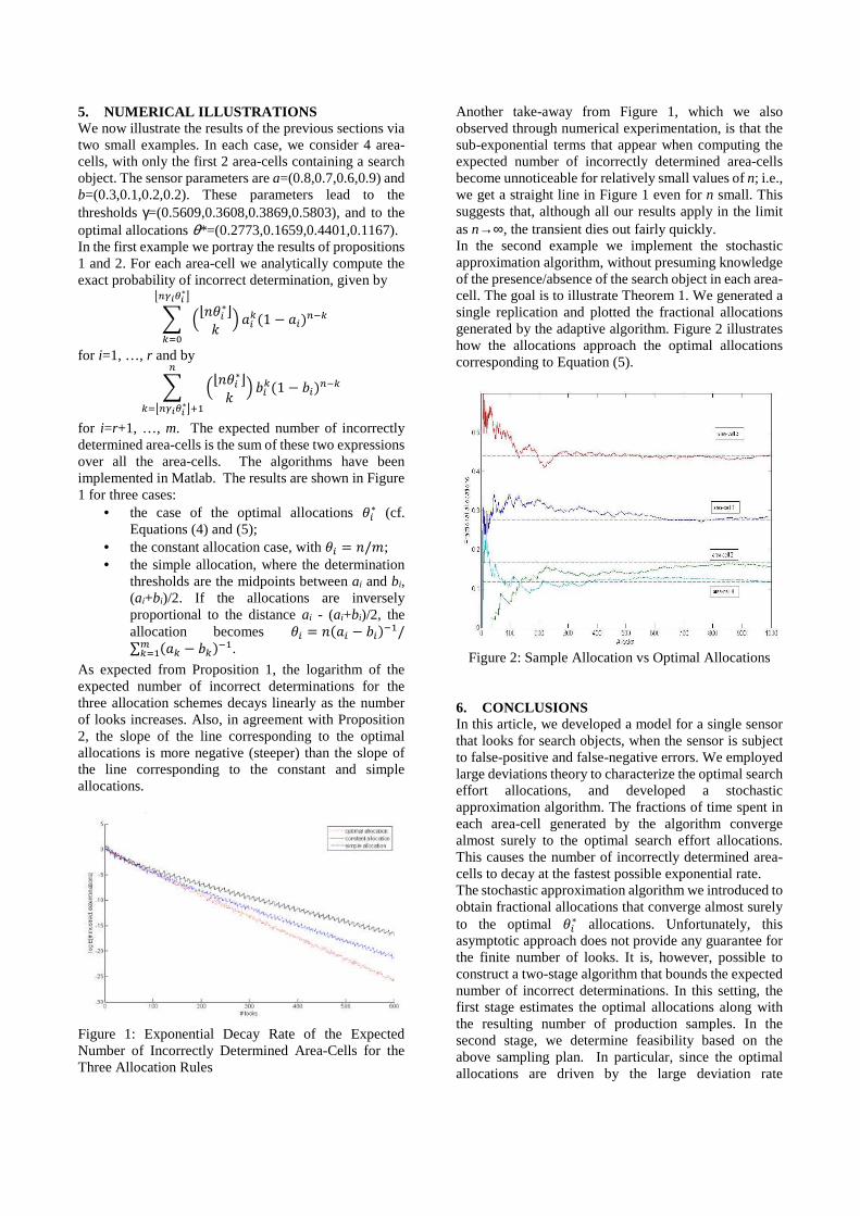
5. NUMERICAL ILLUSTRATIONS We now illustrate the results of the previous sections via two small examples. In each case, we consider 4 area-cells, with only the first 2 area-cells containing a search object. The sensor parameters are a=(0.8,0.7,0.6,0.9) and b=(0.3,0.1,0.2,0.2). These parameters lead to the thresholds γ=(0.5609,0.3608,0.3869,0.5803), and to the optimal allocations θ*=(0.2773,0.1659,0.4401,0.1167). In the first example we portray the results of propositions 1 and 2. For each area-cell we analytically compute the exact probability of incorrect determination, given by

t �u�8�∗vw � Y�a 1 − Y����a

x�-�y�∗z

a�\

for i=1, …, r and by

t �u�8�∗vw � Z�a 1 − Z����a

�

a�x�-�y�∗zB�

for i=r+1, …, m. The expected number of incorrectly determined area-cells is the sum of these two expressions over all the area-cells. The algorithms have been implemented in Matlab. The results are shown in Figure 1 for three cases:

• the case of the optimal allocations 8�∗ (cf. Equations (4) and (5);

• the constant allocation case, with 8� = �/9; • the simple allocation, where the determination

thresholds are the midpoints between ai and bi, (ai+bi)/2. If the allocations are inversely proportional to the distance ai - (ai+bi)/2, the allocation becomes 8� = � Y� − Z����/∑ Ya − Za���<a�� .

As expected from Proposition 1, the logarithm of the expected number of incorrect determinations for the three allocation schemes decays linearly as the number of looks increases. Also, in agreement with Proposition 2, the slope of the line corresponding to the optimal allocations is more negative (steeper) than the slope of the line corresponding to the constant and simple allocations.

Figure 1: Exponential Decay Rate of the Expected Number of Incorrectly Determined Area-Cells for the Three Allocation Rules

Another take-away from Figure 1, which we also observed through numerical experimentation, is that the sub-exponential terms that appear when computing the expected number of incorrectly determined area-cells become unnoticeable for relatively small values of n; i.e., we get a straight line in Figure 1 even for n small. This suggests that, although all our results apply in the limit as n→∞, the transient dies out fairly quickly. In the second example we implement the stochastic approximation algorithm, without presuming knowledge of the presence/absence of the search object in each area-cell. The goal is to illustrate Theorem 1. We generated a single replication and plotted the fractional allocations generated by the adaptive algorithm. Figure 2 illustrates how the allocations approach the optimal allocations corresponding to Equation (5).

Figure 2: Sample Allocation vs Optimal Allocations

6. CONCLUSIONS In this article, we developed a model for a single sensor that looks for search objects, when the sensor is subject to false-positive and false-negative errors. We employed large deviations theory to characterize the optimal search effort allocations, and developed a stochastic approximation algorithm. The fractions of time spent in each area-cell generated by the algorithm converge almost surely to the optimal search effort allocations. This causes the number of incorrectly determined area-cells to decay at the fastest possible exponential rate. The stochastic approximation algorithm we introduced to obtain fractional allocations that converge almost surely to the optimal 8�∗ allocations. Unfortunately, this asymptotic approach does not provide any guarantee for the finite number of looks. It is, however, possible to construct a two-stage algorithm that bounds the expected number of incorrect determinations. In this setting, the first stage estimates the optimal allocations along with the resulting number of production samples. In the second stage, we determine feasibility based on the above sampling plan. In particular, since the optimal allocations are driven by the large deviation rate

functions, we ensure that they are estimated in an accurate fashion. The models developed in this paper may be extended in several directions, including dealing with multiple sensors and considering an arbitrary number of search objects in each area-cell or of a single search object in the area of interest among others. Some of the extensions are presented in Lee (1998). REFERENCES Ahlswede, R., I. Wegener., 1987. Search Problems.

New York: John Wiley. Black, W.L., 1965. Discrete sequential search.

Information and Control, 8:159-162. Breivik, O., Allen, A.A., 2008. An operational search

and rescue model for the Norwegian Sea and the North Sea. Journal of Marine Systems, 69: 99-113.

Chew, M.C., 1967. A sequential search procedure. Annals of Mathematical Statistics, 38: 494-502.

Dembo, A., Zeitouni, O., 1998. Large Deviations Techniques and Applications. New York : Springer-Verlag.

Garcia, A., Campos, E., Li, C., 2005, Distributed online Bayesian search. Proceedings of the International Conference on Collaborative Computing, December 19-22, San Jose (California, USA).

Garcia, A., Li, C., Pedraza, F., 2007. Rational swarms for distributed online Bayesian search. Proceedings of the First International Conference on Robot Communication and Coordination. Athens, Greece.

Kadane, J.B., 1971. Optimal whereabout search. Operations Research, 19: 894-904.

Koopman, B.O., 1946. Searching and Screening. Center for Naval Analysis. Alexandria, VA.

Kress, M,. Szechtman, R., Jones, J.S., 2008. Efficient employment of non-reactive sensors. Military Operations Research.

Kushner, H.J., Yin, G.G., 2003. Stochastic Approximation and Recursive Algorithms and Applications. New York: Springer-Verlag.

Lee, K.K., 2008. Efficient Employment of Adaptive Sensors. Unpublished M.S. Thesis. Department of Operations Research, Naval Postgraduate School. Monterey, CA.

Lehman, E.L., 1986. Testing Statistical Hypotheses. New Yok: John Wiley.

Matula, D. 1964. A periodic optimal search. American Mathematics Monthly, 71: 15-21.

Powell, W.B., 2007. Approximate Dynamic Programming. New York: Wiley.

Ross, S.M. 1983. Introduction to Stochastic Dynamic Programming. New York: Academic Press.

Sato, H., Royset, J.O., 2010. Path optimization for resource-constrained searcher. Naval Research Logistics, 57: 422-440.

Song, N-O., Teneketzis, D., 2004. Discrete search with multiple sensors. Mathematical Methods of Operations Research, 60:1-13.

Stone, L.D. 1975. Theory of Optimal Search. New York: Academic Press.

Szechtman, R., Yücesan, E. 2016. A Bayesian approach to feasibility determination. Proceedings of the Winter Simulation Conference, pp.782-790.

Szechtman, R., Yücesan, E. 2008. A new perspective on feasibility determination. Proceedings of the Winter Simulation Conference, pp.192-199.

Washburn, A.R., 2002, Search and Detection. INFORMS.

Wegener, I., 1980. The discrete sequential search problem with nonrandom cost and overlook probabilities. Mathematics of Operations Research, 5: 373-380.

AUTHORS BIOGRAPHY MOSHE KRESS is a Distinguished Professor of Operations Research at the Naval Postgraduate School (NPS), where he teaches and conducts research in combat modeling and related areas. His current research interests are operations research application in military and defense intelligence, counter-insurgency modeling, homeland security problems, and military logistics. His research has been sponsored by DARPA, ONR, USSOCOM, JIEDDO, USMC and TRADOC. He is the Military and Homeland Security Editor of Operations Research. He published four books and over 75 papers in refereed journals. Dr. Kress has been twice awarded the Koopman Prize for military operations research (2005 and 2009) and the 2009 MOR Journal Award. Prior to joining NPS, Dr. Kress was a senior analyst at the Center for Military Analyses in Israel. He has been a Visiting Professor at the Technion – Israel Institute of Technology, since 2007.

ROBERTO SZECHTMAN received his Ph.D. from Stanford University, after which he joined Oracle Corp. Currently he is Associate Professor in the Operations Research Department at the Naval Postgraduate School. His research interests include applied probability and military operations research, and has been sponsored by ONR, USSOCOM, JIEDDO and TRADOC. He is associate editor for the journals Operations Research, Naval Research Logistics, IIE Transactions, and Transactions on Modeling and Computer Simulation. Professor Szechtman is the 2009 winner of the Koopman Prize for military operations research.

ENVER YÜCESAN is the Abu Dhabi Commercial Bank Chaired Professor of International Management in the Technology and Operations Management Area at INSEAD. He has served as the Proceedings co-editor for WSC'08 and as the Program Chair for WSC'10. He is currently serving as the INFORMS I-Sim representative to the WSC Board of Directors. His research interests include ranking and selection approaches and risk modeling. He holds an undergraduate degree in Industrial Engineering from Purdue University and a doctoral degree in Operations Research from Cornell University.

PROPOSAL ON NETWORK EXPLORATION TO AVOID CLOSED LOOPS

Tatsuya Yamaguchi(a), Tomoko Sakiyama(b), Ikuo Arizono(c)

(a),(c)Graduate School of Natural Science and Technology Okayama University

(b)Faculty of Science and Engineering, Soka University

(a)p6vt8krh@s.okayama-u.ac.jp, (b)sakiyama@soka.ac.jp, (c)arizono@okayama-u.ac.jp

ABSTRACT

There are a lot of enormous networks in the real world,

and it is well-known that Network Exploration is

important to understand structure and connectivity of

the network. A random walk is one of the famous

methods to explore the network. Further, a random walk

is a method of randomly selecting the next node from

one of several adjacent nodes and is frequently used

when a walker can only get local information on the

network. However, since the exploration by a random

walk does not depend on the past exploration process, a

walker on the network enters a loop and therefore visits

the same node several times. In this paper, for

improving the efficiency of network exploration, we

propose an exploration algorithm in which the random

walker selects a passing route as a combination of an

adjacent node and a node two nodes away.

Keywords: network exploring, random walk, scale-free,

complicated networks

1. INTRODUCTION

Networks in the real world are enormous and

complicated such as Web, transportation network, and

neural network of human. Therefore, it is not easy to

investigate an indirect connection from one node to the

specific node. However, it is very important to analyze

these networks in order to grasp vast information (Ikeda,

Kubo, Okumoto and Yamashita 2003). A random walk

is one of an effective and practical method for network

exploration in which the whole image is not found. A

walker with random walk (random walker) explores the

network using only the information on neighboring

connections on the network. During the exploration, the

walker moves to all adjacent nodes with equal

probability because it moves completely randomly.

There are a lot of enormous networks in the real world.

It has been seen that most of the enormous networks in

the real world are “scale-free”. The World Wide Web

(WWW) is a representative example of an enormous

and complicated network. In the case of WWW, each

page is node, and hyperlinks posted on the page form a

network. In fact, WWW has more than 800 million

nodes, and hyperlinks on WWW form a scale-free

network (Barabási and Albert 1999). Then, the number

of nodes connected from a node is called the degree of

the node, and the connection between two nodes is

called the edge. In the scale-free network, the

distribution of degree (degree distribution) obeys a

power-law tailed distribution (Albert and Barabási

2002).

It is well known that Network Exploration is important

to understand structure and connectivity of the network.

A random walk which is a method of randomly

selecting the next node from one of several adjacent

nodes is one of the famous and practical methods to

explore the scale-free network. This means that a

random walk is the exploration algorithm based on only

the local information on the adjacency relation of nodes.

However, since a random walk obeys a Markov process,

the behavior of a random walker is determined by only

the current state and is not affected by past movements.

As a result, that walker during network exploration

enters a loop and goes around a limited area on the

network many times in the scale-free network (Yang

2005; Kim, Park and Yook 2016).

As a feature of the scale-free network, it is known that

there are hub nodes with connecting to many nodes,

since the degree distribution of the scale free network

obeys a power-law. Although a walker at the hub node

can move to a node that has not been visited before,

conversely a walker may also often return to a node that

has already visited. As the exploration time increases,

the number of times the walker has revisited the nodes

which it already visited increases. When the exploration

forms such a loop, it can be said that the exploration

efficiency decreases.

Therefore, in this paper, we consider an exploration

algorithm for improving the efficiency of the scale-free

network exploration. Then, it is necessary to construct

the algorithm behaving adaptively to the scale-free

network feature. Therefore, we propose a modified

random walk algorithm improving the exploration

efficiency through avoiding revisiting the nodes which

the walker has already visited.

In our algorithm, we define nodes connected to adjacent

nodes as virtual adjacent nodes. Then, in addition to the

data on the adjacent node which is the information

utilized in the traditional random walk, the data on the

virtual node is used probabilistically according to the

degree of the current node. Note that in the proposed

algorithm, when the current node has a large degree, the

walker is more likely to move to a node two nodes away.

In this paper, we confirm that the proposed algorithm

has a high exploration efficiency comparing with the

algorithms which do not consider the degree of nodes

including the traditional random walk algorithm.

2. NETWORKS AND RANDOM WALK MODEL

2.1. Networks

We explain networks that are the base of this paper.

Networks are composed of more than one node and one

or more edges which connect the nodes. The total

number of nodes that compose the network is called the

number of nodes N. Moreover, the number of edges

connected each node is called the degree, and the

proportion of the degree k in the whole network is

called degree distribution (Albert, Jeong and Barabási

2000). There are random networks as one of network

construction methods that have been studied since

before. The random network is generated by repeatedly

selecting two nodes from N nodes randomly and

connecting the nodes with a constant probability p .

Figure 1 is an example of the random network. In this

figure, a circle represents a node, and its size represents

the degree of the node. Generally, it is known that

Poisson distribution explains the degree distribution of

random networks (Barabási and Albert 1999, Albert and

Barabási 2002).

Whereas, the degree distribution of the most networks

in the real world is different from the random network

and does not follow Poisson distribution. Concretely,

the degree distribution ( )P k of network in the real

world can be represented based on the power-law as

follows:

( ) ~P k k (2.1)

where denotes the scaling index. Then, considering

the networks in the real world, we have the scaling

index as 1 3 (Albert and Barabási 2002). The

property that the order distribution ( )P k of a network

is expressed by a power law is called scale-free property

of the network, and the network with scale-free property

is called scale-free network. Figure 2 is an example of

the Scale-free network.

2.2. Random Walk

The random walk model is known as the typical and

practical method to explore the path from the start to the

goal on the network to understand structure and

connectivity of the network (Noh and Rieger 2004). The

walker in the random walk model moves to an adjacent

node among all adjacent nodes with the equal

probability. It is a useful method when the network

connection near each node is known. The probability

ijP that the walker moves from node i to node j is

represented as

Figure 1: Random Network

Figure 2: Scale-free Network

1

, ,

0, ,

i

iij

j N kkP

otherwise

(2.2)

where ik and iN k indicate the degree of node i and

the population of the nodes adjacent to node irespectively. The walker in the random walk model

moves to an adjacent node of adjacent nodes according

to Eq. (2.2) one by one. It is completely random that the

walker moves to which node among adjacent nodes, and

even though the walker has visited a node once, the

walker moves to the node with the same probability as

other nodes. For this reason, a random walk has a

problem that the walker tends to draw a loop especially

when positioned on nodes with large degree. To

improve this problem, we propose the “Skip Model” in

the next section. We explore on the random network

and the scale free network by using the random walk

model and the proposed model and verify the

effectiveness of the proposed model.

3. PROPOSAL OF SKIP MODEL

In this section, we introduce the Skip Model as a

proposed model in this paper. The basic exploring

method of this model is almost the same as the random

walk model. However, although the walker in the

random walk model moves to the adjacent nodes

according to equation (2.2) basically, the Skip Model

has a feature that the walker in the Skip Model

sometimes moves to two nodes away node passing the

adjacent nodes with the following probability lQ

specified based on the degree lk of node l :

11 .l

l

Qk

(3.1)

For instance, the probability lmnP that the walker at node

l move to two nodes away node n passing the adjacent

node m is represented as follows:

1 1 1

1 ,1

0, .

l m

lmn l l m

m N k and n N kP k k k

otherwise

(3.2)

Note that lk and

mk are the degrees of node l and m

respectively. In addition, note that if the node where the

walker is located and the node which is two nodes away

are directly connected by an edge, i.e. nodes l , m and

n form a triangle, the walker does not move to node n .

According to Eq. (3.1), in the event of using the Skip

Model, the larger the degree of the node where the

walker is located is, the higher the probability of

moving to the node which is two nodes away is. In this

way, it would be possible to avoid forming closed loops

that increases exploring time by moving to the node

which is two nodes away at the node which has large

degree. We call this model of moving to the node which

is two nodes away with the defined probability in Eq.

(3.1) the Skip Model.

For comparisons, we prepare the Skip1 Model fixed as

1lQ and The Skip0.5 Model fixed as 0.5lQ . It is

found that the Skip1 Model is a model that always

moves two by two and the Skip0.5 Model is a model

that moves two with the constant probability of 1/2.

Furthermore, the model becomes the traditional random

walk if we set as 0lQ . Hence, we call the traditional

random walk model as the Skip0 Model in this paper.

We explore the network by using these four models and

look for the best method among them.

4. EXPERIMENT

In this section, we analyze the exploration on the two

networks explained in section 2 by using the four

models introduced in section 3 while changing the

scaling index and the number of nodes N . Then, we

calculate the average exploring times from the obtained

data, evaluate the significant difference of the result of

each model, and indicate the effectiveness of the Skip

Model regarding the solution ability of the problem.

4.1. Experimental Conditions

First, we explain the flow of the experiment. We

generated a random network and scale-free network

described in section 2 and decided the start and goal

randomly. We explored 10 times each on the network with same start node and goal node by using the Skip

Model, the Skip0.5 Model, the Skip1 Model, and the

Skip0 Model described in section 3. We tried these

processes 1000 times, found the average exploring

times from the start to the goal for each model, and

calculated the significant difference of performance of

the Skip Model by using Mann-Whitney U-test and

analysis of variance (ANOVA). However, if the walker

had not reached the goal even though the walker moves

1000 times, we counted it as the number of unreached

times.

Regarding generating the networks, we generated

random networks by repeating the operation of selecting

two nodes randomly and connecting them with

probability p . Then, we set the probability 1.0p . On

the other hand, we generated scale-free networks

according to the power law of Eq. (2.1). Concretely, the

scale-free networks generated while changing the scale

index to 1.0 and 2.0 in this experiment.

4.2. Experimental results

Most networks in the real world are scale-free.

Therefore, we show the results of exploring the scale-

free network, first. After that, the results of exploring

the random network are shown.

4.2.1. Scale-free Networks

First, we show the exploring results for scale-free

networks in Tables 1 and 2, and Figures 3 and 4. Table

1 and Figure 3 show the results of exploring the scale-

free network with the scaling index 1.0 , and Table 2

and Figure 4 show the results with 2.0 . According

to Table 1 and Figure 3, the Skip0 Model which is

random walk always takes 1.5 times longer than the

other models regardless of the value N , and it is

significantly inferior. Similarly, the Skip1 Model is

inferior to the Skip Model and the Skip0.5 Model

regardless of the value of N . The Skip Model is the

best under the conditions of 100N and 200N ,

however inferior to the Skip0.5 Model under the

condition of 300N .

Table 2 and Figure 4 show that the Skip0 Model is

inferior to the other models at all N values as in the

case of 1.0 . The Skip0.5 Model is inferior to the

other models under the condition of 200N , and the

Skip1 Model is inferior to the other models under the

condition of 300N . On the other hand, the Skip

Model is superior to the other models at all value of N .

Table 3 shows that the number of times which the

walker does not reach the goal after moving 1000 times.

According to Table 3, the Skip0 Model is significantly

inferior to the other models in respect to the number of

unreached times as with average exploring time.

Moreover, the Skip Model and the Skip1 Model have

similar values for all N and . The Skip0.5 Model is

inferior to the other models except the condition of

100N and 1.0 . Considering comprehensively the

results in Tables 1 and 2, and Figures 3 and 4, it can be

seen that the Skip Model has the superior exploration

ability in comparison to the other models for all N and

.

Table 1: The Average Exploring Times on the Scale-

free Network Under condition of 1.0

N Skip Skip0.5 Skip1 Skip0

100 79.2 86.8 86.9 150

200 149 151 154 249

300 204 194 209 307

Figure 3: The Result of exploring on the Scale-free

Network Under Condition of 1.0

Table 2: The Average Exploring Times on the Scale-

free Network Under condition of 2.0

N Skip Skip0.5 Skip1 Skip0

100 91.5 98.0 96.4 175

200 159 171 165 260

300 204 207 218 311

Figure 4: The Result of Exploring on the Scale-free

Network Under Condition of 2.0

Table 3: The Number of Unreached Times on the

Scale-free Network N Skip Skip0.5 Skip1 Skip0

1.0

100 40 25 70 106

200 142 234 164 757

300 422 574 424 1466

2.0

100 53 77 70 260

200 337 454 325 1019

300 654 814 657 1756

4.2.2. Random Networks

Next, we show the results for exploring on the random

network in Table 4 and Figure 5. The Skip0 Model

which is the random walk model is inferior to the other

models as with the results on the scale-free network.

Although the Skip0.5 Model is slightly inferior to the

Skip Model and the Skip1 Model, there is no big

difference concerning these models which pass through

the adjacent nodes. In addition, we show the number of

unreached times for respective models in Table 5. By

making a comparison between Table 3 and 5, it is

obvious that the number of unreached times in the

random network is less than those in the scale-free

network regarding any model and value of N . The

number of unreached times for each model in the

random network is almost the same results for the Skip

Model and the Skip1 Model, but the Skip0.5 Model is

inferior to the above-referenced two models, and the

Skip0 Model is inferior to the other three models.

Table 4: The Average Exploring Times on the Random

Network

N Skip Skip0.5 Skip1 Skip0

100 74.1 76.8 73.7 124

200 130 134 129 205

300 181 184 181 259

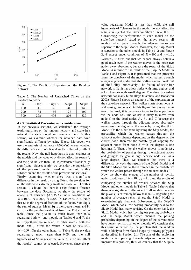
Figure 5: The Result of Exploring on the Random

Network

Table 5: The Number of Unreached Times on the

Random Network

N Skip Skip0.5 Skip1 Skip0

100 1 50 31 146

200 134 166 125 497

300 298 406 303 839

4.2.3. Statistical Processing and consideration

In the previous sections, we calculated the average

exploring times on the random network and scale-free

network for each model and compare them. In this

section, we examine whether the obtained data have

significantly different by using U-test. Moreover, we

use the analysis of variance (ANOVA) to see whether

the differences in models and in the value of affect

the results. Now, the null hypothesis is that “changes in

the models and the value of do not affect the results”,

and the p-value less than 0.05 is considered statistically

significant. Subsequently, we consider the superiority

of the proposed model based on the test in this

subsection and the results of the previous subsections.

Firstly, examining whether there was a significant

difference in the result by using U-test, the p-values for

all the data were extremely small and close to 0. For this

reason, it is found that there is a significant difference

between the data. Secondly, we show the results of

analysis of variance (ANOVA) under conditions of

100N , 200N , 300N in Tables 6, 7, 8. Note

that Df is the degree of freedom of the factor, Sum Sq is

the sum of squares, Mean Sq is the square mean, and Pr

(> F) is the p-value evaluated from the F distribution

table. Since the p-value is much lower than 0.05

regarding both and models in Tables 6 and 7, the

null hypothesis are rejected. In other words, both the

model and affect the results in case of 100N ,

200N . On the other hand, in Table 8, the p-value

regarding much larger than 0.05, and the null

hypothesis of “changes in the value of do not affect

the results” cannot be rejected. However, since the p-

value regarding Model is less than 0.05, the null

hypothesis of “changes in the model do not affect the

results” is rejected also under condition of 300N .

Considering the performance of each model on the

scale-free network based on the above results, all

models which pass through the adjacent nodes are

superior to the Skip0 Model. Moreover, the Skip Model

is superior to the other models in Table 1, 2 and Figure

3, 4 except under condition of 300N and 1.0 .

Whereas, it turns out that we cannot always obtain a

good result even if the walker moves to the node two

nodes away absolutely, because the result of the Skip1

Model is inferior to the result of the Skip0.5 Model in

Table 1 and Figure 3. It is presumed that this proceeds

from the drawback of the model which passes through

always adjacent nodes that the walker cannot break out

of blind alley immediately. The feature of scale-free

network is that it has a few nodes with large degree, and

a lot of nodes with small degree. Therefore, scale-free

network has many blind alleys (Barabási and Bonabeau

2003). Figure 6 shows an example of the exploration on

the scale-free network. The walker starts from node S

and must go to node G in this figure. For the walker to

reach the goal, it is necessary to go to the upper node

via the node M . The walker is likely to move from

node S to the dead nodes A , B , and C because the

walker passes through the adjacent nodes absolutely

regardless the degree of the node by using the Skip1

Model. On the other hand, by using the Skip Model, the

probability which the walker passes through the

adjacent nodes change depending on the degree of the

current node, therefore the possibility of skipping the

adjacent nodes from node S with the degree is one

becomes 0. Then, after the walker moves to node M ,

the probability of passing through the adjacent nodes

and going to the goal is high because node M has a

large degree. Thus, we consider that there is a

difference between the results of the Skip1 Model and

the Skip Model due to the difference in the probability

which the walker passes through the adjacent nodes.

Now, we show the average of the number of revisits

under conditions of 100N , 1.0 , and the results of

comparing the number of revisits between the Skip

Model and other models in Table 9. Table 9 shows that

there is a significant difference for all models because

the p-value is extremely below than 0.05. Regarding the

number of average revisit times, the Skip0 Model is

overwhelmingly frequent. Subsequently, the Skip0.5

Model which has a low passing probability next to the

Skip0 Model has many revisits. On the other hand, the

Skip1 Model which has the highest passing probability

and the Skip Model which changes the passing

probability depending on the degree of the current node

have fewer revisits than other models. We consider that

this result is caused by the problem that the random

walk is likely to form closed loops by drawing polygons

as described in Section 2.1. The aim of the exploring

model which passing through adjacent nodes is to

improve this problem, thus we can say that the Skip0.5

Model is inferior to the Skip Model. Moreover, since

the Skip0.5 Model has a lot of unreached times next to

the Skip0 Model, we can infer that these two models are

prone to fall into closed loops compared with the Skip

model and the Skip1 Model in Figure 4.1.

On the random network, the Skip0 Model is inferior to

the models which pass through adjacent nodes as with

scale-free network as shown in Tables 4-8 and Figure 5.

the Skip0.5 Model is inferior to the Skip Model in

respect to the average exploring time and the number of

unreached times, however there is no significant

difference between the Skip1 Model and the Skip

Model. The problem which the walker is likely to fall

into closed loops also occurs on the random network,

and it is improved by the model which passing through

adjacent nodes. Hence, the Skip0 Model (i.e., random

walk) and the Skip0.5 Model are inferior to the Skip

Model and the Skip1 Model. On the other hand, we

infer that there is no large difference about the result

between the Skip Model and the Skip1 Model because

random networks have few nodes which have small

degrees compared with scale-free networks and have

few blind alleys.

Summarizing the results in Tables 1, 2, 3 and Figures 3,

4 and considerations, it is concluded that the Skip

Model which is proposed model is superior on the

whole to the other models on the scale-free network

from the viewpoint of the average exploring time, the

number of unreached times, and the number of revisit

times, on the whole. Regarding the random network, the

Skip0 Model and the Skip0.5 Model are inferior to the

other models. Further, there is no large difference

between the Skip Model and the Skip1 Model. After all,

it can be concluded that the Skip Model is relatively

useful compared to other models.

Table 6: The Result of ANOVA on the Scale-free

Network ( 100N )

Df Sum

Sq

Mean

Sq

F-

value

Pr (>F)

1 421 420.5 16.71 0.02646

Model 3 7988 2662.6 105.81 0.00153

Residual 3 75 25.2

Table 7: The Result of ANOVA on the Scale-free

Network ( 200N )

Df Sum

Sq

Mean

Sq

F-value Pr (>F)

1 338 338 30.73 0.011575

Model 3 13975 4658 423.47 0.000194

Residual 3 33 11

Table 8: The Result of ANOVA on the Scale-free

Network ( 300N )

Df Sum

Sq

Mean

Sq

F-value Pr (>F)

1 85 85 5.227 0.106325

Model 3 16095 5365 331.845 0.000279

Residual 3 48 16

Figure 6: An Example of Exploring on the Scale-free

Network

Table 9: The Number of Revisit Times on the Scale-free

Network ( 100N , 1.0 )

Skip Skip0.5 Skip1 Skip0

p-value - 16

2.20

10

16

2.20

10

16

2.20

10

average 3.10 4.59 2.48 9.82

5. CONCLUSION

The random walk is one of the famous exploring

methods in respect to the exploration of complex

networks. However, a random walk has the problem

that the walker falls into frequently closed loops and

affects exploring time. To solve this problem, we

proposed the Skip Model that increased or decreased the

skipping probability depending on the degree of the

current note considering the structure that closed loops

had been formed in networks in this paper. Furthermore,

we created two models with constant skip probability,

and verified four exploring models including the

traditional random walk model.

Consequently, the Skip Model is superior to the other

models frequently regarding the average exploring

times on the scale-free network. The Skip Model is the

best methods for the number of nodes and scaling index

verified this time because the number of unreached

times is not many even under conditions where average

exploring times is inferior. Focusing on the problem of

forming closed loops which is our initial aim, the Skip

Model has far fewer revisits than random walk, and the

number of unreached times is superior to the other

models. Therefore, it can be said that this model does

not solve the problem completely, however improves it

significantly. Meanwhile, the three models which pass

through the adjacent nodes have a new problem that the

walker cannot break out of blind alley immediately. The

Skip1 Model which is an excellent model on the

random network is affected by this problem heavily,

and the results of the model on the scale-free network

are not good. On the other hand, by using the Skip

Model, the probability of passing through the adjacent

nodes changes appropriately according to the degree of

the node. Therefore, the result of the model is excellent

on the scale-free network.

The Skip Model is the most effective exploring method

regardless of the type of network, the number of nodes,

and the value of under the conditions of examined in

this paper. Nevertheless, networks in the real world

have a lot of nodes not within the number of nodes used

in this paper. Furthermore, scaling index changes to

various values depending on the networks. To adopt the

Skip Model as one of the exploring methods on

complex networks, it will be necessary to verify on the

networks which have a lot of nodes and consider the

results.

ACKNOWLEDGMENT

This work was supported by Japan Society for the

Promotion of Science (JSPS) KAKENHI Grant Number

18K04611: “Evaluation of system performance and

reliability under incomplete information environment”.

We would like to appreciate the grant for our research.

REFERENCES

Barabási A.-L., and Albert R., 1999. Emergence of

scaling in random networks. Science, 286(5439),

509-512.

Albert R., Jeong H., and Barabási A.-L., 2000. Error

and attack tolerance of complex networks. Nature,

406, 378-382.

Yang S.-J., 2005, Exploring complex networks by

walking on them. Physical Review E, 71(1).

Ikeda S., Kubo I., Okumoto N., and Yamashita M.,

2003. Impact of local topological information on

random walks on finite graphs. Automata,

Languages and Programming, 1054-1067.

Kim Y., Park S, and Yook S.-H., 2016. Network

exploration using true self-avoiding walks.

Physical Review E, 94(4).

Barabási a.-l., and Bonabeau E., 2003. Scale-Free

Networks. Scientific American, 288(5), 60-69.

Albert R., and Barabási A.-L., 2002. Statistical

mechanics of complex networks. Reviews of

Modern Physics, 74(1), 47-97.

Noh J.-D., Rieger H., 2004. Random walks on complex

networks. Physical review letters, 92(11).

Biographical notes: Tatsuya Yamaguchi was born in

Okayama, Japan on 1996 July 15. He received the BE

from Okayama University in the Department of

Mechanical and Systems Engineering in 2019. He is a

student in the Graduate School of Natural and

Technology, Okayama University, and he will receive

the ME from Okayama University in the Graduate

School of Natural and Technology in 2021. His research

interests center in the Exploring Complicated Network.

Tomoko Sakiyama received the BE, the ME and the

PhD from Kobe University, all in the Department of

Earth and Planetary Sciences, in 2012, 2013 and 2015,

respectively. From 2016 to 2018 she was an Assistant

Professor in the Graduate School of Natural and

Technology, Okayama University. From 2019, she is an

Associate Professor in the Faculty of Science and

Engineering, Soka University. Her research interests

center in the Swarm Intelligence.

Ikuo Arizono was born in Osaka, Japan on 1959 Feb

22. He received the BE, the ME and the PhD from

Osaka Prefecture University, all in the Department of

Industrial Engineering, in 1982, 1984 and 1988,

respectively. From 1985 to 1990 he was a Research

Associate, from 1990 to 1994, an Assistant Professor

and since 1994, an Associate Professor in the Graduate

School of Engineering, Osaka Prefecture University.

From 2011, he is a Professor in the Graduate School of

Natural and Technology, Okayama University. His

research interests center in the Statistical Quality

Control and Operational Research.

JOB SHOP RESCHEDULING WITH LOT SPLITTING

UNDER MULTIPLE INTERRUPTIONS

Takuya Okamoto(a), Yoshinari Yanagawa(b), Ikuo Arizono(c)

(a),(b),(c) Graduate school of Natural Science and Technology, Okayama University, Japan.

(a)pcvy55zs@s.okayama-u.ac.jp, (b)yanagawa.y@okayama-u.ac.jp, (c)arizono@.okayama-u.ac.jp

ABSTRACT

Production does not necessarily process on schedule. In

fact, it is sometimes that works are stopped by some

causes of machine breakdowns and so on. When these

situations have occurred, rescheduling is made out to

reduce bad influence. This is mostly executed by using

RSS (Right-Shift-Scheduling) or metaheuristics such as

GA (Genetic Algorithm). However, metaheuristics and

RSS have drawbacks. In this research, we would propose

a new rescheduling method using lot splitting. When the

interruption happens in a factory, a time lag between

machining start time at the beginning and the end of a lot

exists in the following factory. We think that the time lag

makes it possible to split the lot into two sublots with an

appropriate ratio and the delivery into two. As a result,

our proposed method is not inferior to GA and is superior

to RSS under the evaluation of the number of tardy jobs.

Keywords: job shop scheduling, lot splitting,

rescheduling, setup time

1. INTRODUCTION

Over the years, production scheduling has been studied

in order to keep the due date, to reduce the cost and so

on. Previous researches have suggested effective

methods by simulating under supposing various

situations. However, unexpected events such as

interruptions of works or additions of new jobs may

occur in actual situations. Pinedo (2008) have stated the

12 principal differences between the simulation model

and the real scheduling problem:

1. New jobs constantly arrive in the system.

2. The rescheduling problem is important.

3. The job environments are more complicated.

4. The weights (priorities) of jobs change with

time.

5. Job preferences in the selection of machines are

important.

6. There are restrictions in machine availability

according to working shift patterns or

timetables.

7. Nonlinear penalty functions.

8. Several objectives are often considered.

9. Overtime work and working time assignment of

workers depend on the amount of work and the

time margin.

10. Processing times do not follow statistical

distributions.

11. Processing times on the same machine tend to

be highly positively correlated.

12. Processing time distributions may be subject to

change due to learning or deterioration.

From the above, it is necessary to handle a situation that

takes into consideration more realistic conditions. For

example, operation stopping is often happened because

of some causes of machine breakdowns and so on. Other

unexpected situations such as machine failure, change in

due date (changed earlier), addition of jobs, etc. may

always occur. When such situations occur, the initial

production schedule is reorganized, which is called

Rescheduling, in order to reduce bad influence of the

operation stopping. Rescheduling is a combination

problem. Therefore, it is often solved with metaheuristics

such as GA. Metaheuristics can get an optimal solutions

or values close to them. However, in fact, it takes time to

get a new schedule for the operation of renewing input

data at every interruption, and it is almost difficult to trust

the output of metaheuristics because of the unclear

deriving method and process. Therefore, rescheduling is

very likely made by RSS.

RSS is a method of shifting the initial schedule backward

for the interruption time as it is. RSS has an advantage

which is not to need newly considering the setup time,

however, is greatly affected by interruption time. In the

case that idle time is large, RSS is effective because of

the interruption time is absorbed by the idle time in

factory. However, idle time is usually set small because

idle time is mostly dead time. So, since the work

interruption time is usually much longer than the idle

time, RSS cannot fully take its effectiveness.

In this research, we propose a new lot splitting method

alternative to GA and RSS. Generally, a job is the set of

works to make products, and the lot is a part of a job and

the set of work to make products. Our proposed method

is that a specific lot at an interruption is split into two

sublots and the sublots are separately send to the

succeeding factory, respectively. Considering the

handling of the product in the succeeding factory, there

is a time lag in process start time between the start part

and the end part of the original lot. Once a part of the lot

has been delivered, the succeeding factory can start

processing. We think that it is possible to reduce the

overall due date tardiness if the time lag is used to

process the first delivery lot in a succeeding factory and

the undelivered part of the lot is processed by machines

in an interrupted factory. Through comparing the

proposed method with GA and RSS which are

conventionally used, we confirm the effectiveness in

rescheduling of the proposed method.

2. PREVIOUS RESEARCHS

2.1. Scheduling Environment

Production scheduling problems are roughly split into the

flow shop problems and the job shop problems. The

former means a problem in which all jobs are processed

in the same order, and the latter means a problem in

which the order of machines for processing is different

for each job.

For an example in the flow shop problem, Katragjini et

al. (2012) have proposed a solution for problems with

different interrupting factors. The solution in Katragjini

et al. (2012) is to reschedule the original schedule when

some events such as a machine failure, appearance of a

new job, or change at processing start time are happened

in the flow shop problem. They propose ways have

quality and reliability by using the IG (Iterated Greedy)

(Ruiz and Stützle 2007).

On the other hand, here are some examples of the job

shop problem. Sarker et al. (2016) have proposed a

method of minimizing the make span by using IMA

(Improves Memetic Algorithm) which is a type of GA

when a new job is assigned. Jiang et al. (2016) have

proposed a method to acquire production information in

real time by using IoT and suppress the influence on total

processing time. They use the evolved form of ACO (Ant

Colony Optimization) called IACO (Improved Ant

Colony Optimization) when a rescheduling is needed due

to the machine failure. Also, Vieira et al. (2003) have summarized and reported

some of other rescheduling methods which were studied.

2.2. Lot Splitting

A lot is a processing unit to make products and a part of

a job. The lot size can be changed to an arbitrary size as

necessary, and it is possible to prevent excessive

inventory and out-of-stock by appropriately controlling

the lot size. Since the size of the lot very likely influence

the total processing time, it is also considered in the

production scheduling problem. For example, Low et al.

(2003) have proposed a method to minimize the make-

span by splitting a lot into several sublots. The size of all

sublots were equalized and some sublots added in the

paper. However, they also have stated that there are

drawbacks that margin of schedule improvement

decrease or costs increase if the number of sublots is

increased excessively. Haase and Kimms (2000)

proposed a method of rescheduling with reduced idle

time by adjusting the lot size of original schedule.

However, they don’t consider unexpected situations such

as work interruptions. On the other hand, as far as we

know, there is no study that assumes splitting lots to cope

with the interruption of works.

3. PROPOSED MODEL

In this research, we consider splitting lots to cope with

the interruption of works. At this time, we think that

flexibility in rescheduling can be secured by performing

lot splitting when interruption occurred. In this research,

we propose a method of performing lot splitting at the

time of work interruption and performing rescheduling

by applying the dispatching rule described later.

3.1. Model Setting

The model dealt with in this research is set as follows:

1. Job shop problem is treated which have 10 jobs

and 10 machines.

2. The setup time of a job is given depending on

each machine and the preceding job.

3. In one machine only one job is processed at a

time.

4. The unit of time is minutes.

5. The workable start times of all jobs are set time

0.

6. The worktime per a day is set 480 and the

planning horizon is 5 days.

7. Due date differs depending on the job, and it is

generated between 1300 and 2400 with uniform

random numbers.

8. All jobs are only processed once on each

machine.

9. The work time of each product is set depending

on each process, and they are generated between

1 and 5 with uniform random numbers.

10. One job consists of one lot.

11. The lot size which means the number of

products is set depending on each job, and it is

generated between 20 and 60 with uniform

random numbers.

12. The slack time is between 20% and 50% of the

duration from the feasible production start time

of each job to the due date.

13. No more than one machine is interrupted at any

time, and the interruptions are occurred with

uniform random numbers.

14. Two types of interruption timing are treated.

Interruption of work shall be set with uniform

random numbers either at the start time of a

workday or immediately at the end of a lunch

break. Specifically, it is (0 or 240), (480 or 720),

(960 or 1200), (1440 or 1680) and (1920 or

2160). The numbers in the parenthesis show the

candidate for the timing of each interruption

occurrence.

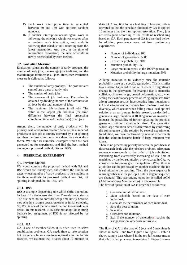
15. Each work interruption time is generated

between 60 and 150 with uniform random

numbers.

16. If another interruption occurs again, work is

following the schedule which was created after

a previous work interruption, and work is

following that schedule until returning from the

latest interruption. And then, at the time of

interruption restoration, the new schedule is

newly rescheduled by each method.

3.2. Evaluation Measure

Evaluation values are the number of tardy products, the

number of tardy jobs, the average jobs tardiness, and the

maximum job tardiness in all jobs. Here, each evaluation

measure is defined as follows:

The number of tardy products: The products are

sum of tardy parts of tardy jobs

The number of tardy jobs

The average of job tardiness: The value is

obtained by dividing the sum of the tardiness for

all jobs by the total number of jobs.

The maximum job tardiness in all jobs: The

value is the largest job tardiness (the time

difference between the final processing

completion time and the due date) of all jobs.

Among them, the number of tardy products will be

primary evaluated in this research because the number of

products in each job is directly operated by a lot splitting

and then the time criterion is considered as a secondary

factor. We solve 40 numerical examples which are data

generated us for experiment, and find the best method

among our proposed method, GA and RSS.

4. NUMERICAL EXPERIMENT

4.1. Previous Method

We would compare the proposed method with GA and

RSS which are usually used, and confirm the number of

cases whose number of tardy products is the smallest in

the three methods. In proposed method and GA, lot

splitting is adopted, but in RSS, isn't.

4.1.1. RSS

RSS is a simple dispatching rule which shifts operations

backward for the interruption time. The rule has a priority.

The rule need not to consider setup time newly because

new schedule is same operation order as initial schedule.

So, RSS is one of the most used method to reschedule in

actual. In this research, RSS dose not adopt lot splitting

because job assignment of RSS is not affected by lot

splitting.

4.1.2. GA

GA is one of metaheuristics. It is often used to solve

combination problems. GA needs time to take solution

but can get a solution close to an optimal solution. In this

research, we estimate that it takes about 10 minutes to

derive GA solution for rescheduling. Therefore, GA is

operated so that the schedule obtained by GA is applied

10 minutes after the interruption restoration. Then, jobs

are reassigned according to the result of rescheduling

based on GA. Each parameter of GA is described below.

In addition, parameters were set from preliminary

experiments.

Number of individuals: 100

Number of generations: 5000

Crossover probability: 70%

Mutation probability: 1%

Large mutation event: at the 1000th generation

Mutation probability in large mutation: 50%

A large mutation is to suddenly raise the mutation

probability once at a specific generation. This is similar

to a situation happened in nature. It refers to a significant

change in the ecosystem, for example due to meteorite

collision, climate change, crustal deformation, etc., when

seeing the evolutionary process of living organisms from

a long-term perspective. Incorporating large mutations in

GA is due to prevent individuals from the loss of solution

diversity, which occurs when falling into a local optimal

solution at an early stage. In this research, we decided to

generate a large mutation at 1000th generation in order to

increase the possibility of further updating the previous

generated optimum solution is raised. The generation

where large mutation occur is determined by confirming

the convergence of the solution by several experiments.

In addition, we have confirmed by several experiments

that the solution became better if large mutation was

taken.

There is no processing priority between the jobs because

this research deals with the job shop problem. Also, gene

sequence corresponds to the order of job submission.

Preventing from excessively increasing of idle time of

machines by the job submission order created in GA, we

consider the following gene manipulation. When there is

a job that can be processed by another machine, the job

is submitted to the machine. Then, the gene sequence is

rearranged because the job input order and gene sequence

are changed. This rearranging operation is called AGM

(Additional Gene Manipulation) in this research.

The flow of operation of GA is described as follows:

1. Generate initial individuals.

2. Make schedule based on the data of each

individual.

3. Calculate the performance of each individual.

4. Save the best solution.

5. Selection.

6. Crossover and mutation.

7. Exit if the number of generations reaches the

last generation, otherwise return to 2.

The flow of GA in the case of 5 jobs and 5 machines is

shown in Table 1 and from Figure 1 to Figure 5. Table 1

shows sample data where 5 in the top left corner means

that job 1 is first processed in machine 5. Figure 1 shows

an example of GA solution. In Figure 1, the numbers

from 1 to 5 in the sequence mean jobs which are assigned

to machines in order from the left. In Figure 1, the 1st

process of job 1 is assigned into the leftist locus, and then

the 1st operation of job 4 is assigned into the 2nd leftist

locus. The second 3 which appears in the 6th leftist locus

means the 2nd operation of job 3. Figure 2 and Figure 3

show the example schedule obtained based on Table 1

and Figure 1. Figure 2 shows job assignment to each

machine from leftist locus 1 to 6. Figure 3 shows that all

jobs are assigned according to the locus. Figure 4 shows

the gene sequence of Figure 1 rearranged by AGM. In

Figure 4, for example, the 7th locus is changed from 2 to

4. In addition, the 10th, 11th, 12th, 13th, 14th, 16th, 17th, 18th,

20th and 21st loci are changed. Each evaluation measure

of each individual is calculated from the solution and the

best solution of the generation is saved. And the best

solution is kept until a better solution being generated. In

the crossover procedure, two-point crossover and

mutation are executed to generate children. The flow of

the two-point crossover is as follows and shows in Figure

5. Firstly, two solutions are selected as parents from the

solutions, and it is determined whether to cross the

parents or not according to the crossover probability.

When crossover is executed, two cut points are randomly

selected. Job numbers between two cut points in the

selected parents are compared and the job numbers are

swapped between the parents. When the number of some

jobs is excess and other jobs is deficient after the

crossover, the number of excess and deficient jobs is only

adjusted by swapping the jobs each other from the leftist

side in the swapped numbers. And then, mutation would

be executed. The solution of GA is the best solution at

the final generation.

Table 1: Sample Processing Data

Operation Number

1st 2nd 3rd 4th 5th

Job

Number

1 5 3 2 4 1

2 1 5 4 3 2

3 2 5 3 1 4

4 3 5 2 1 4

5 2 4 5 1 3

Figure 1: Example of an Individual

Figure 2: Example of Assigning Jobs According from 1st to 6th locus

Figure 3: Example of GA Schedule

Figure 4: Example of Rearranged Individual by AGM

Figure 5: Two-Point Crossover

4.2. Proposed Method

It is inevitable that an interruption occurs in production

activities, and how to suppress the effect of the

interruption is important. In the past researches mostly

focused only on the site where the interruption took place

and an initial schedule is rescheduled to be able to deal

with the interruption on the interrupted workstation.

However, it is rare to make products from the beginning

to the end within one factory. Products are made through

processes in multiple companies and work sites.

Therefore, if an interruption occurs in a factory, the

interruption likely affects all related factories. In such a

case, the succeeding factory will be negotiated about the

due date and delivery of the affected products. In this

research, we pay attention to the fact that the negotiation

is carried out, and assume that some specific lots can be

split into 2 sublots, that is, sublot 1 and sublot 2. Then,

sublot 1 which is delivered at the initial due date and the

other sublot 2 which is permitted delivering with a little

tardiness. In this research, we will treat 3 patterns about

delaying due date of sublots 2: same due date as initial

lots (pattern 1), delay 10% of initial lots (pattern 2), and

delay 20% of initial lots (pattern 3). Sublots 1 have

processing priority to other unsplit lots and sublots 2. The

simple flow of the proposed method is shown as follows:

1. Initial schedule is created by EDD (Earliest due

date) or GA.

2. Select the lots to be split at the time of an

interruption (details of lot splitting will be

described later).

3. Split the selected lots into sublots 1 and sublots

2, respectively.

4. Apply the corresponding dispatching rule with

consideration for the recovery time until the

time of the interruption recovery, and perform

rescheduling.

5. Repeat steps 2 to 4 when another interruption

occurs.

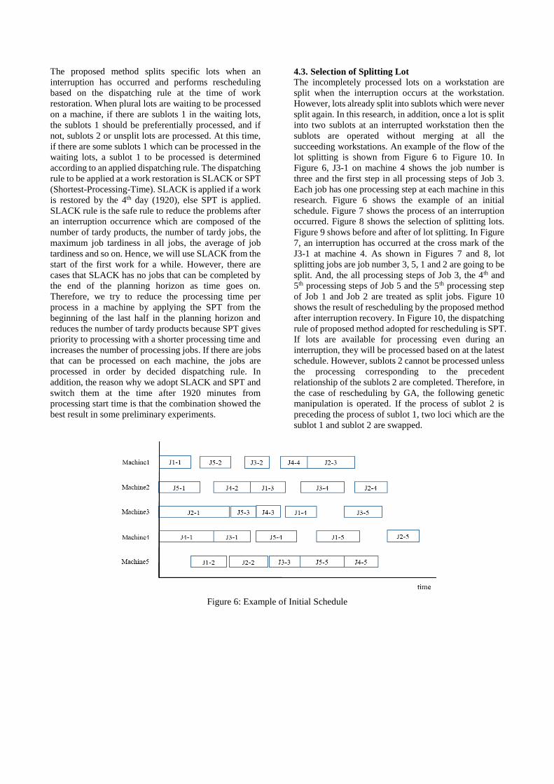
The proposed method splits specific lots when an

interruption has occurred and performs rescheduling

based on the dispatching rule at the time of work

restoration. When plural lots are waiting to be processed

on a machine, if there are sublots 1 in the waiting lots,

the sublots 1 should be preferentially processed, and if

not, sublots 2 or unsplit lots are processed. At this time,

if there are some sublots 1 which can be processed in the

waiting lots, a sublot 1 to be processed is determined

according to an applied dispatching rule. The dispatching

rule to be applied at a work restoration is SLACK or SPT

(Shortest-Processing-Time). SLACK is applied if a work

is restored by the 4th day (1920), else SPT is applied.

SLACK rule is the safe rule to reduce the problems after

an interruption occurrence which are composed of the

number of tardy products, the number of tardy jobs, the

maximum job tardiness in all jobs, the average of job

tardiness and so on. Hence, we will use SLACK from the

start of the first work for a while. However, there are

cases that SLACK has no jobs that can be completed by

the end of the planning horizon as time goes on.

Therefore, we try to reduce the processing time per

process in a machine by applying the SPT from the

beginning of the last half in the planning horizon and

reduces the number of tardy products because SPT gives

priority to processing with a shorter processing time and

increases the number of processing jobs. If there are jobs

that can be processed on each machine, the jobs are

processed in order by decided dispatching rule. In

addition, the reason why we adopt SLACK and SPT and

switch them at the time after 1920 minutes from

processing start time is that the combination showed the

best result in some preliminary experiments.

4.3. Selection of Splitting Lot

The incompletely processed lots on a workstation are

split when the interruption occurs at the workstation.

However, lots already split into sublots which were never

split again. In this research, in addition, once a lot is split

into two sublots at an interrupted workstation then the

sublots are operated without merging at all the

succeeding workstations. An example of the flow of the

lot splitting is shown from Figure 6 to Figure 10. In

Figure 6, J3-1 on machine 4 shows the job number is

three and the first step in all processing steps of Job 3.

Each job has one processing step at each machine in this

research. Figure 6 shows the example of an initial

schedule. Figure 7 shows the process of an interruption

occurred. Figure 8 shows the selection of splitting lots.

Figure 9 shows before and after of lot splitting. In Figure

7, an interruption has occurred at the cross mark of the

J3-1 at machine 4. As shown in Figures 7 and 8, lot

splitting jobs are job number 3, 5, 1 and 2 are going to be

split. And, the all processing steps of Job 3, the 4th and

5th processing steps of Job 5 and the 5th processing step

of Job 1 and Job 2 are treated as split jobs. Figure 10

shows the result of rescheduling by the proposed method

after interruption recovery. In Figure 10, the dispatching

rule of proposed method adopted for rescheduling is SPT.

If lots are available for processing even during an

interruption, they will be processed based on at the latest

schedule. However, sublots 2 cannot be processed unless

the processing corresponding to the precedent

relationship of the sublots 2 are completed. Therefore, in

the case of rescheduling by GA, the following genetic

manipulation is operated. If the process of sublot 2 is

preceding the process of sublot 1, two loci which are the

sublot 1 and sublot 2 are swapped.

Figure 6: Example of Initial Schedule

Figure 7: Interruption Occurrence

Figure 8: Selection of Splitting Lots

Figure 9: Lot Splitting of Selected Part

Figure 10: Example of Rescheduling by Proposed Method after Interruption Recovery

5. RESULTS OF NUMERICAL EXPERIMENTS

AND CONSIDERATION

In this research, all sublots 2 in proposed method and GA

are allowed to miss their initial due date, but in RSS, the

due date is fixed same as initial due date. Table 2 shows

the results in case of that initial schedules of proposed

method and RSS are made by EDD, and Table 3 shows

the results in case of that initial schedules of proposed

method and RSS are made by GA. GA is superior to other

two methods in most patterns from each pattern in upper

parts of Table 2 and 3. In particular, GA is very excellent

in pattern 1. However, the proposed method is as good as

GA in pattern 2 and pattern 3. The reason is considered

that GA is not able to perform fully the potential when

the diversity of solutions is impaired as the progress of

processes. Also, it is considered that GA is affected

critically when conditions of machine processability are

changed from the latest schedule because GA calculates

the best or near the best schedule at each timing of

rescheduling. So, scheduling by GA suffers fatal damage

on the specific situations and tends to leave delayed jobs

to process. On the other hand, the proposed method is

considered not to be affected than GA because it

schedules jobs according to rules established in advance

even when the conditions are changed from the latest

schedule. Although the proposed method has situations

not to be treated, it can reduce serious job tardiness

because of switching the dispatching rule adopted

depending on the elapsed time of processing.

Then, we consider the rate of delaying the due date of

sublots 2. The result of scheduling by GA is improved as

delay the due date of sublots 2. However, in proposed

method, it is not to say that simply delaying due date of

sublots 2 is better. This is caused by that SLACK affects

the results largely. In the proposed method, SLACK is

applied at rescheduling executed from the start of

processing to 1920 minutes (the time is the fourth day

ends). The delay of the due date of sublot 2 can change

the processing priority by SLACK. Therefore, if

rescheduling is performed on the 3rd and 4th days, the

case can occur that a job which remains only one process

is delayed because SLACK gives priority to jobs with

less margin of due date. This phenomenon can occur as

the due date of sublot 2 is delayed more, and in the

proposed method, pattern 2 is superior to pattern 3 in

some cases. From the above, it is considered that the

proposed method needs to change the dispatching rules

to be applied according to the rate of delaying the due

date of sublots 2.

As a result, the proposed method is inferior to GA from

upper parts of Table 2 and 3. However, the result is not

so bad from average of each evaluation measures in

lower part of Table 2 and 3. And then, it can be an

alternative of GA for rescheduling when time, labor on

workshop and reliability from workers are taken into

consideration. Moreover, the rate of delaying the due

date of sublots 2 depend on the interruption time, but it

is considered impractical to delay 20% of initial due date

or more. Also, in this research, the due date of sublots 2

are delayed uniformly, but the limits of delaying due date

of sublots 2 are actually different by each job. If the

conditions are changed as described above, the results are

different, so it is necessary to further experiments.

Table 2: The Results of Numerical Experiments (The Initial Schedule of Proposed Method and RSS is made by EDD)

Table 3: The Results of Numerical Experiments (The Initial Schedule of Proposed Method and RSS is made by GA)

Proposed

MethodGA RSS

Proposed

MethodGA RSS

Proposed

MethodGA RSS

15 34 0 15 17 0 21 31 0

18 38 1 20 20 1 22 31 0

15 32 0 14 16 0 21 31 0

22 23 2 13 16 2 22 30 0

41.55 16.05 137.35 10.9 9.05 137.35 13.45 5.075 137.35

2.3 0.975 3.975 0.725 0.625 3.975 0.85 0.45 3.975

40.4975 12.9175 247.8375 8.5175 4.975 247.8375 11.1275 2.3275 247.8375

169.9 151.95 482.375 62.025 73.4 482.375 69.125 45.075 482.375

Pattern1 Pattern2 Pattern3

The Number of

Minimum Cases in

40 Cases

The Number of Tardy Products

The Number of Tardy Jobs

The Average of Job Tardiness

The Maximum Job Tardiness in All Jobs

Average Value of

40 Cases

The Number of Tardy Products

The Number of Tardy Jobs

The Average of Job Tardiness

The Maximum Job Tardiness in All Jobs

Proposed

MethodGA RSS

Proposed

MethodGA RSS

Proposed

MethodGA RSS

18 30 5 17 17 4 23 30 5

18 36 6 20 20 6 23 30 4

17 28 5 16 16 3 22 30 4

24 20 6 15 16 3 22 30 4

32 16.05 107.525 10.825 9.05 90.35 14.35 5.075 107.525

1.9 0.975 3.65 0.675 0.625 3.325 0.8 0.45 3.65

29.195 12.9175 64.17 8.9825 4.975 53.475 12.3225 2.3275 64.17

144.725 151.95 318.8 57.275 73.4 313.55 87.85 45.075 318.8

Pattern1 Pattern2 Pattern3

Average Value of

40 Cases

The Number of Tardy Products

The Number of Tardy Jobs

The Average of Job Tardiness

The Maximum Job Tardiness in All Jobs

The Number of

Minimum Cases in

40 Cases

The Number of Tardy Products

The Number of Tardy Jobs

The Average of Job Tardiness

The Maximum Job Tardiness in All Jobs

6. CONCLUTION

In this research, we proposed a rescheduling method

using lot splitting under the multiple work interruptions.

We compare our method with GA and RSS about the

number of tardy products, the number of tardy jobs, the

average jobs tardiness, and the maximum job tardiness in

all jobs. RSS does not split lots because the order of

processing is not changed, but GA splits lots to bring the

conditions closer to the proposed method. The proposed

method is not so inferior to GA but greatly superior to

RSS. The main reason is that proposed method is less

affected than GA under multiple interruptions. In

addition, the effectiveness of the proposed method

increased with the ratio of delaying the due date of the

sublots 2. So, the proposed method very likely have a

potential to be superior to GA depending on time

constraints. Also, GA has the disadvantage that extra

works are required on sites and workers don’t trust the

solution. From the above, the proposed method is

considered to be an alternative to GA etc.

As future prospects, we would like to suppose an

experimental model closer to the actual situation and

brush up the proposed method to exceed the results of

GA.

REFERENCES

Haase K. and Kimms A., 2000. Lot sizing and scheduling

with sequence-dependent setup costs and items and

efficient rescheduling opportunities. International

Journal of Production Economics, 66: 159-169

Jiang Y., Ding Q., and Wang X., 2016. A recovery model

for production scheduling: Combination of

disruption management and Internet of Things.

Scientific Programming, 2016: Article ID 8264879,

9 pages, doi.org/10.1155/2016/8264879.

Katragjini K., Vallada E. and Ruiz R., 2013. Flow shop

rescheduling under different types of disruption.

International Journal of Production Research, 51

(3): 780-797.

Low C., Hsu C. and Huang K., 2004. Benefits of lot

splitting in job-shop scheduling. International

Journal of Advanced Manufacturing Technology,

24(9-10): 773–780.

Ruiz R. and Stützle T, 2007. A simple and effective

iterated greedy algorithm for the permutation

flowshop scheduling problem. European Journal of

Operational Research, 177 (3): 2033–2049.

Sarker R., Essam D., Hassan S.M.K. and Karim A. N. M.,

2016. Managing risk in production scheduling

under uncertain disruption. Artificial Intelligence

for Engineering Design, Analysis and

Manufacturing, 30 (3): 289–299.

Vieira G.E., Herrmann J.W., and Lin E., 2003.

Rescheduling manufacturing system: A framework

of strategies, policies, and methods. Journal of

Scheduling, 6 (1): 39-62.

Pinedo M. 2008. Scheduling: Theory, algorithms and

systems. 3rd ed. New York: Springer.

AUTHORS BIOGRAPHY

Takuya Okamoto was born in Okayama, Japan on 1995

July 10. He received the BE from Okayama University

in the Department of Mechanical and Systems

Engineering in 2018. He is a student in the Graduate

School of Natural and Technology, Okayama University,

and he will receive the ME from Okayama University in

the Graduate School of Natural and Technology in 2020.

His research interests center in the Production

Rescheduling.

Yoshinari Yanagawa was born in Hyogo, Japan on 1964

Feb 19. He received the BE and the ME in the

Department of Industrial Engineering from Osaka

Prefecture University in 1987 and 1989, respectively. He

also received the PhD in Engineering from Okayama

University in 1994. From 1990 he belongs to Okayama

University and he is an Associate Professor in the

Graduate School of Natural and Technology, Okayama

University from 2005. His research interests are in

Production management and Resource management.

Ikuo Arizono was born in Osaka, Japan on 1959 Feb 22.

He received the BE, the ME and the PhD from Osaka

Prefecture University, all in the Department of Industrial

Engineering, in 1982, 1984 and 1988, respectively. From

1985 to 1990 he was a Research Associate, from 1990 to

1994, an Assistant Professor and since 1994, an

Associate Professor in the Graduate School of

Engineering, Osaka Prefecture University. From 2011,

he is a Professor in the Graduate School of Natural and

Technology, Okayama University. His research interests

center in the Statistical Quality Control and Operational

Research.

A NOVEL FIREFLY ALGORITHM FOR MULTIMODAL OPTIMIZATION

Masato Kondo(a), Tomoko Sakiyama(b), Ikuo Arizono(c)

(a), (c)Graduate School of Natural Science and Technology, Okayama University

(b) Faculty of Science and Engineering, Soka University

(a)pnpl2vnj@s.okayama-u.ac.jp, (b)sakiyama@soka.ac.jp, (c)arizono@okayama-u.ac.jp

ABSTRACT

Firefly Algorithm (FA) has a high ability for inquiring an

optimal solution in Optimization Problem. However, FA

cannot find multiple solutions including an optimal

solution in Multimodal Optimization Problems. Multimodal Optimization Problem which is one of

optimization problems demands finding all or most of the

multiple solutions as well as the best solution. It is very

important to inquire many alternatives when an optimal

solution is unavailable.

Therefore, we propose New Firefly Algorithm which has

new functions for Multimodal Optimization. In this

model, agents realize searching solutions in multiple

region and adjust parameters related to the search range

of objective function regardless of the shape of the

objective function. The model can have an ability for

finding an optimal solution and suboptimal solutions. We

applied conventional FA and proposed FA to multimodal

objective functions and found that proposed FA was

superior to conventional FA for Multimodal

Optimization Problems.

Keywords: Firefly Algorithm, Multimodal Optimization

Problem, Swarm intelligence

1. INTRODUCTION

Among evolutionary computation algorithms, Swarm

intelligence such as Firefly Algorithm (FA), Particle

Swarm Optimization (PSO) and Ant Colony

Optimization (ACO) are inspired from the collective

behavior of animal. These algorithms have powerful

performance for solving Optimization Problems

(Kennedy and Eberhart 1995; Dorigo 1997).

Especially, FA invented by Yang (2008) inspired from

some of the flashing characteristics of fireflies (Yang

2008). Since then, several improvements of the FA have

been devised (Yang 2018). The conventional FA was

applied to the continuous optimization problems.

Currently however, it has been applied to many other

problems, for instance, the discrete optimization

problems, multi-objective optimization problems and so

on (Yang 2013; Marichelvam et al. 2014; Marichelvam

and Geetha 2016). Therefore, the conventional FA and

its extended algorithms have the potential to be applied

to more various applications in the future.

In this study, we address to develop a novel FA that has

an ability for finding an optimal solution and suboptimal

solutions simultaneously. In the future, this study will

widen the application range of the FA algorithms.

Conventional FA by Xing-She Yang is basically known

as a technique for searching a best solution in the search

range of objective function.

On one hand, among some types of optimization

problems, Multimodal Optimization Problems demand

finding all or most of the multiple solutions as well as the

best solution. For example, in the case of proposing a best

route with car navigation, we must set alternative

suboptimal route under circumstances where an optimal

route cannot be used by traffic jams or accidents.

Therefore, it is very important to inquire many

alternatives when an optimal solution is unavailable.

However, conventional FA by Xing-She Yang is

basically known as a technique for searching a best

solution in the search range of objective function.

Although conventional FA can occasionally obtain a few

solutions in multiple region, it cannot inquire

simultaneously many solutions (Yang 2008). Therefore,

there is room for improvement of the performance of FA

because this algorithm does not have any high

performance for multimodal optimization problems.

Hence, in this paper, we propose a new FA for

multimodal optimization problems. Concretely, we

address to develop a novel FA that has an ability for

finding an optimal solution and suboptimal solutions

simultaneously. In the proposed model, agents realize

searching solutions in multiple region and adjust

parameters related to the search scale regardless of the

shape of the objective function. As a result, the model

can have an ability for finding an optimal solution and

suboptimal solutions simultaneously. In the future, this

study will widen the application range of the FA

algorithms.

2. FIREFLY ALGORITHM

In this section, we describe Firefly Algorithm (FA)

according to Yang (2008). FA obeys following three

rules simplified some of the characteristics of real

fireflies:

• All fireflies are unisex so that one firefly will be

attracted to other fireflies regardless of their sex.

• Attractiveness of each firefly is proportional to

their brightness, thus for any two flashing

fireflies, the less bright one will move towards

the brighter one. • The brightness of a firefly is affected or

determined by the landscape of the objective

function.

In maximum optimization problems, Light intensity

iI of a firefly i is calculated as follows:

( ),i iI f x= (1)

where ( )if x is an objective function while ix indicates

the current position of firefly i .

On the other hand, in minimum optimization problems,

Light intensity of a firefly i is calculated as follows in

order to avoid the denominator of the function is zero:

( )1

min ( ) 1 .i iI f f x−

= − + (2)

Parameter minf represents the best solution in an

objective function.

Initial position of each firefly is based on random

location within the search range of an objective function.

A less bright firefly will move towards the brighter one.

But, the approaching distance is based on attractiveness

of the brighter firefly. Attractiveness is based on the

nature of light.

In general, the light obeys Beer-Lambert law and light

intensity decreases exponentially by absorbing light into

the air. In addition, the light intensity at the distance d

from the light source is based on Inverse-square law

which is inversely proportional to the square of the

distance. Therefore, considering Beer-Lambert law and

Inverse-square law, Light intensity I is defined as

follows:

( )2

0( ) exp .I d I d= − (3)

Here, is light absorption coefficient and 0I is the light

intensity at a light source respectively. Parameter d

represents the distance from the light source.

Therefore, attractiveness of firefly j for firefly i can be

defined as follows:

( )2

0 exp .ij ijr = − (4)

Here, ijr indicates the Euclidean distance between agent

i and j while 0 represents attractiveness at 0ijr = .

And ijr is defined as follows:

2

1

( ) .D

ij i j ik jk

k

r x x x x=

= − = − (5)

Here, D is the number of dimensions in the Euclidean

space.

Based on attractiveness ij of another more attractive

firefly j , the movement of a firefly i is determined by

( ) ,i i ij j i ix x x x = + − + (6)

Where is randomization parameter and determines

scale of random walk and i means random number

based on uniform distribution or Gaussian distribution.

In eq.(6), second term is related to localized interactions

and multiple regions of search and third term means

random walk.

Pseudo code of FA is shown in Figure 1.

Objective function ( )f x , 1( , , )T

dx x=x

Generate initial population of fireflies ( 1, , )ix i d=

Light intensity iI at

ix is determined by ( )if x

Define light absorption coefficient

while t MaxGenaration do

Sort fireflies in ascending order of light intensity

for 1:i n= all n fireflies do

for :j i n= all n fireflies do

if i jI I then

Move firefly i towards j in d-dimension based on eq.(6)

end if

end for

end for

Find the current best

end while

Postprocess results and visualization

Figure 1: Pesudo code of FA

3. FISSION-FUSION FIREFLY ALGORITHM

In this section, we describe the novel Firefly Algorithm

for Multimodal Optimization Problems.

This model is named Fission-Fusion Firefly Algorithm

(FFFA), because of behaviors where fireflies divide from

groups or gather in groups.

In addition to three rules of FA, FFFA is based on

following three rules.

• While FA is a synchronous algorithm, FFFA is

an asynchronous algorithm.

• The flash rate of each firefly is based on the

Euclidean distance between each firefly and

their N th adjacent firefly. One firefly with

high flash rate does not interact with one with

low flash late.

• A firefly interacts with adjacent fireflies based

on the Euclidean distance or adjacent fireflies

based on Light intensity by switching condition.

• The parameters related to search scale are based

on distance of Nth adjacent firefly.

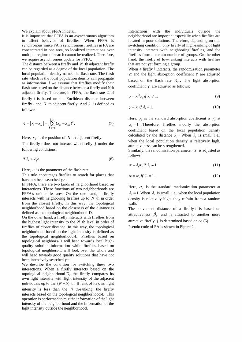
We explain about FFFA in detail. It is important that FFFA is an asynchronous algorithm

to affect behavior of fireflies. When FFFA is

synchronous, since FA is synchronous, fireflies in FA are

concentrated in one area, so localized interactions over

multiple regions of search cannot be realized. Therefore,

we require asynchronous update for FFFA.

The distance between a firefly and N th adjacent firefly

can be regarded as a degree of the local population. The

local population density names the flash rate. The flash

rate which is the local population density can propagate

as information if we assume that fireflies modify their

flash rate based on the distance between a firefly and Nth

adjacent firefly. Therefore, in FFFA, the flash rate i of

firefly i is based on the Euclidean distance between

firefly i and N th adjacent firefly. And i is defined as

follows:

2

1

( ) .D

i i N ik Nk

k

x x x x=

= − = − (7)

Here, Nx is the position of N th adjacent firefly.

The firefly i does not interact with firefly j under the

following conditions:

.i jif (8)

Here, is the parameter of the flash rate.

This rule encourages fireflies to search for places that

have not been searched yet.

In FFFA, there are two kinds of neighborhood based on

interactions. These functions of two neighborhoods are

FFFA's unique features. On the one hand, a firefly

interacts with neighboring fireflies up to N th in order

from the closest firefly. In this way, the topological

neighborhood based on the closeness of the distance is

defined as the topological neighborhood-D.

On the other hand, a firefly interacts with fireflies from

the highest light intensity to the N th level in order of

fireflies of closer distance. In this way, the topological

neighborhood based on the light intensity is defined as

the topological neighborhood-L. Fireflies based on

topological neighbors-D will head towards local high-

quality solution information while fireflies based on

topological neighbors-L will look over the whole and

will head towards good quality solutions that have not

been intensively searched yet.

We describe the condition for switching these two

interactions. When a firefly interacts based on the

topological neighborhood-D, the firefly compares its

own light intensity with light intensity of the adjacent

individuals up to the ( )N + th. If rank of its own light

intensity is less than the N th-ranking, the firefly

interacts based on the topological neighborhood-L. This

operation is performed to mix the information of the light

intensity of the neighborhood and the information of the

light intensity outside the neighborhood.

Interactions with the individuals outside the

neighborhood are important especially when fireflies are

located in poor solutions. Therefore, depending on this

switching condition, only firefly of high-ranking of light

intensity interacts with neighboring fireflies, and the

fireflies form a certain number of groups. On the other

hand, the firefly of low-ranking interacts with fireflies

that are not yet forming a group.

When a firefly i interacts, the randomization parameter

and the light absorption coefficient are adjusted

based on the flash rate i . The light absorption

coefficient γ are adjusted as follows:

2 1.i s iif = (9)

1.s iif = = (10)

Here, s is the standard absorption coefficient is s at

1i = .Therefore, fireflies modify the absorption

coefficient based on the local population density

calculated by the distance i . When i is small, i.e.,

when the local population density is relatively high,

attractiveness can be strengthened.

Similarly, the randomization parameter is adjusted as

follows:

1.i s iif = (11)

1.s iif = = (12)

Here, s is the standard randomization parameter at

1i = .When i is small, i.e., when the local population

density is relatively high, they refrain from a random

walk.

The movement distance of a firefly i is based on

attractiveness ij and is attracted to another more

attractive firefly j is determined based on eq.(6).

Pseudo code of FA is shown in Figure 2.

Objective function ( )f x , 1( , , )T

dx x=x

Generate initial population of fireflies ( 1, , )ix i d=

Light intensity iI at ix is determined by ( )if x

Define the standard randomization parameter s

Define the standard light absorption coefficient s

Upper limit of the adjacent fireflies N

while t MaxGenaration do

Sort randomly fireflies i

for 1:i n= all n fireflies do

Calculate the all flash rate i based on eq.(7)

A firefly can see light intensity based on eq.(8)

Adjust the parameters and based on eq.(9) and (11)

Calculate the rank iR of light intensity in fireflies up to the

( )N + th adjacent firefly

if iN R then

for 1:j N= sorted all N fireflies

in ascending order of light intensity do

if i jI I then

Move firefly i towards j in d-dimension based on eq.(6)

in the topological neighborhood-D

end if

end for

else

for :j i N= sorted all N fireflies

in ascending order of light intensity do

if i jI I then

Move firefly i towards j in d-dimension based on eq.(6)

in the topological neighborhood-L

end if

end for

end if

end for

Find the current best

end while

Postprocess results and visualization

Figure 2: Pseudo code of FFFA

4. RESULTS

4.1. Experimental conditions

In this research, we apply FFFA to the objective function

of various shapes and evaluate its performance. Formulas

of the objective function are shown on eq.(10), (11) and

(12). 2 2 2 2

1 2 1 2

2 2 2 21 2 1 2

( 4) ( 4) ( 4) ( 4)

1 2

( 4)

1 2

1( , )

2 ,

5 , 5.

x x x x

i

x x x x

F x x e x e

e e

x x

− − − − − + − −

− − − − +

= +

+ +

−

(13)

1 2

2 2

1 2 1 2

1 2

2( , ) 80

10cos(2 ) 10sin(2 ) 20 ,

5.12 , 5.12.

F x x

x x x x

x x

=

− + − − +

−

(14)

2

1 1

1 2

2

2 2

1 2

4 53( , ) exp 2log 2 sin

8 2

4 5exp 2log 2 sin ,

8 2

5 , 5.

x xF x x

x x

x x

+ + = −

+ + + −

−

(15)

Shapes of the objective functions F1, F2 and F3 are

shown in Figures 3, 4 and 5. In addition, the values of the

solutions are shown in Tables 1, 2 and 3. We use the

objective functions F1, F2 and F3 where there are

multiple solutions and we know those solutions exactly.

Objective functions are modified so that all search ranges

are aligned to avoid tuning the parameters of FA and they

can be handled as maximum optimization problems.

Figure 3: The shape of F1

Table 1: The values of the solutions in F1

The value of

the solution

The Position

1x 2x

2.0 0.0 0.0

2.0 0.0 -4.0

1.0 4 4

1.0 -4 4

Figure 4: The shape of F2

Table 2: The values of the solutions in F2

The value of

the solution

The Position

1x 2x

80.0 0.0 0.0

79.0 0.0 1.0

79.0 0.0 -1.0

79.0 1.0 0.0

79.0 -1.0 0.0

78.0 1.0 1.0

78.0 1.0 -1.0

78.0 -1.0 -1.0

78.0 -1.0 -1.0

Figure 5: The shape of F3

Table 3: The values of the solutions in F3

The value of

the solution

The Position

1x 2x

2.0 -4.0 -4.0

Table 4 and 5 show Parameters in FA and FFFA

respectively.

Table 4: The Parameter of FA

Parameter The set value

𝛽0 1.0

𝛼 0.2

𝛾 1.0

Table 5: The Parameter of FFFA

Parameter The set value

N 5

δ 3

𝛾𝑠 0.004

𝛼𝑠 1.0

ε 0.25

𝛽0 1.0

In FA and FFFA, the number of steps is set to 500, the

number of trials is set to 100, the number of agents is set

to 50. We use Mersenne twister as a pseudo random

number generator for random walk in the experiments

(Matsumoto and Nishimura 1998).

4.2. Validation on ability for finding an optimal

solution

In this section, we compare the found rate of optimal

solutions of objective function in FA and FFFA. We use

the multimodal objective functions (F1, F2 and F3)

where there are multiple local solutions. The finding

condition of the optimal solution is the time when a

solution within an error of 0.005 is found from the

coordinates of the point where the optimal solution is

located. In each trial, Table 6 shows the results of the

found rate of optimal solutions. As shown in Table 6, the

found rate of the optimal solution of FFFA is higher than

that of FA. Therefore, FFFA for multimodal optimization

problems realizes the improvement of solving ability of

optimal solution.

Table 6: The found rate of optimal solutions

Function The found rate (%)

FA FFFA

F1 100 100

F2 13 99

F3 79 100

4.3. Validation on ability for finding multiple

solutions

In this section, we compare the found number of the

multiple solutions of the objective function in FFFA and

FA. We use the multimodal objective functions (F1 and

F2, where there are multiple solutions and we know those

solutions exactly). The finding condition of the optimal

solution is the time when a solution within an error of

0.005 is found from the coordinates of the point where

the solution is located. In each trial, Table 7 shows the

results of the found number of multiple solutions.

As shown in Table 7, the found number of the multiple

solutions of FFFA is more than that of FA.

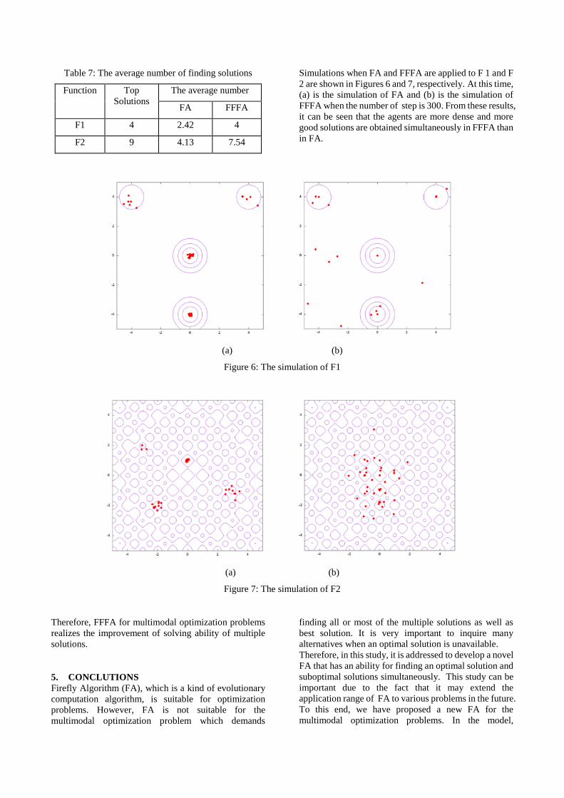
Table 7: The average number of finding solutions

Function Top

Solutions

The average number

FA FFFA

F1 4 2.42 4

F2 9 4.13 7.54

Simulations when FA and FFFA are applied to F 1 and F

2 are shown in Figures 6 and 7, respectively. At this time,

(a) is the simulation of FA and (b) is the simulation of

FFFA when the number of step is 300. From these results,

it can be seen that the agents are more dense and more

good solutions are obtained simultaneously in FFFA than

in FA.

(a) (b)

Figure 6: The simulation of F1

(a) (b)

Figure 7: The simulation of F2

Therefore, FFFA for multimodal optimization problems

realizes the improvement of solving ability of multiple

solutions.

5. CONCLUTIONS

Firefly Algorithm (FA), which is a kind of evolutionary

computation algorithm, is suitable for optimization

problems. However, FA is not suitable for the

multimodal optimization problem which demands

finding all or most of the multiple solutions as well as

best solution. It is very important to inquire many

alternatives when an optimal solution is unavailable.

Therefore, in this study, it is addressed to develop a novel

FA that has an ability for finding an optimal solution and

suboptimal solutions simultaneously. This study can be

important due to the fact that it may extend the

application range of FA to various problems in the future.

To this end, we have proposed a new FA for the

multimodal optimization problems. In the model,

fireflies realize searching solutions in multiple region

and adjust parameters related to the search scale

regardless of the shape of the objective function. In

addition, the model makes it possible for the firefly to

rebuild the group at a better solution place by forming

and dissolution of groups by Switching between two

neighbors. The model is called Fission-Fusion Firefly

Algorithm (FFFA), because of behaviors where fireflies

divide from groups or gather in groups.

From the experimental results for validation on ability

for finding an optimal solution and multiple solutions,

the proposed model has an ability for finding an optimal

solution and suboptimal solutions.

REFERENCES

Yang X.S., 2008. Nature-Inspired Metaheuristic

Algorithms, Luniver Press.

Yang X.S., 2018. Nature-Inspired Algorithms and

Applied Optimization, Springer.

Marichelvam M.K., Parabaharan T., Yang X.S., 2014. A

discrete firefly algorithm for the multiobjective

hybrid flowshop schefuling problems, IEEE

Transactions on Evolutionary Computation, vol.18,

no.2, pp.301-305.

Marichelvam M.K., Geetha M., 2016. A hybrid discrete

firefly algorithm to solve flow shop sheduling

problems to minimise total flow time, Int. J. Bio-

inspired Computation, vol.8, no.5, pp.318-325.

Yang X.S., 2013. Multiobjective firefly algorithm for

continuous optimization, Engineering with

Computers, vol. 29, no.2, pp. 36-50.

Kennedy J., Eberhart., 1995. Particle swarm optimization.

Proceedings of the 1995 IEEE International

Conference on Neural Networks, vol.4, pp. 1942–

1948.

Dorigo M., 1997. Ant Colony System: A Cooperative

Learning Approach to the Traveling Salesman

Problem. IEEE Transactions on Evolutionary

Computation, vol. 1, no. 1, pp. 1-24.

Matsumoto M., Nishimura T., 1998. Mersenne Twister:

A 623-dimensionally equidistributed uniform

pseudorandom number generator. ACM

Transactions on Modeling and Computer

Simulation, vol. 8, no. 1, pp.3-30.

AUTHORS BIOGRAPHY

Biographical notes: Masato Kondo was born in

Okayama, Japan on 1995 Aug 8. He received the BE

from Okayama University in the Department of

Mechanical and Systems Engineering in 2018. He is a

student in the Graduate School of Natural and

Technology, Okayama University, and he will receive

the ME from Okayama University in the Graduate

School of Natural and Technology in 2020. His research

interests center in Swarm Intelligence.

Tomoko Sakiyama received the BE, the ME and the

PhD from Kobe University, all in the Department of

Earth and Planetary Sciences, in 2012, 2013 and 2015,

respectively. From 2016 to 2018 she was an Assistant

Professor in the Graduate School of Natural and

Technology, Okayama University. From 2019, she is an

Associate Professor in the Faculty of Science and

Engineering, Soka University.

Her research interests center in the Swarm Intelligence.

Ikuo Arizono was born in Osaka, Japan on 1959 Feb 22.

He received the BE, the ME and the PhD from Osaka

Prefecture University, all in the Department of Industrial

Engineering, in 1982, 1984 and 1988, respectively. From

1985 to 1990 he was a Research Associate, from 1990 to

1994, an Assistant Professor and since 1994, an

Associate Professor in the Graduate School of

Engineering, Osaka Prefecture University. From 2011,

he is a Professor in the Graduate School of Natural and

Technology, Okayama University. His research interests

center in the Statistical Quality Control and Operational

Research.

1

COMPUTATIONAL INVESTIGATION ON THE EFFECT OF VARIOUS PARAMETERS

OF A SPIRAL GROUND HEAT EXCHANGER

Lazaros Aresti(a), Paul Christodoulides(b), Lazaros Lazari(c), Georgios A. Florides(d)

(a) Department of Electrical Engineering, Computer Engineering and Informatics, Cyprus University of Technology,

Limassol, Cyprus (b), (d) Faculty of Engineering and Technology, Cyprus University of Technology, Limassol, Cyprus

(c) Department of Mechanical Engineering and Materials Science and Engineering, Cyprus University of Technology,

Limassol, Cyprus

(a)lg.aresti@edu.cut.ac.cy, (b)paul.christodoulides@cut.ac.cy, (c)lazaros.lazaris@cut.ac.cy, (d)georgios.florides@cut.ac.cy

ABSTRACT

Shallow Geothermal Energy, a Renewable Energy

Source, finds application through Ground Source Heat

Pumps (GSHPs) for space heating/cooling via tubes

directed into the ground. Vertical Ground Heat

Exchangers (GHEs) of various configurations (mainly

U-tubes) extract/reject heat into the ground. Spiral type

GHEs constitute an alternative to reduce the depth and

hence the cost of GSHP systems. Such GHEs are used in

energy piles, which are reinforced concrete foundations

with helical pipes whereby heating/cooling is provided.

Testing GHEs through experimental set-ups is expensive

and time consuming. Hence, a computational

investigation is preferred. To this end the current paper

introduces a 3D mathematical model, based on the

convection-diffusion equation, in COMSOL

Multiphysics. The related parameters are adjusted, and

the model is validated, against experimental data. The

validated model is subsequently adapted to match the

Cyprus moderate Mediterranean conditions. A

parametric investigation of the important implications in

the design of GHEs is also conducted.

Keywords: Ground Heat Exchanges, Spiral GHE,

COMSOL validation

1. INTRODUCTION

Renewable Energy Systems (RES) have increased in

popularity in recent years through a global effort to divert

away from fossil fuels and reduction of CO2. Such a

system is Ground Source Heat Pump (GSHP), which

takes advantage of the Geothermal Energy stored in the

sublayers of the earth. GSHP systems are used for space

heating and cooling, where heat is either extracted or

rejected to the earth using a network of tubes directed

into the ground.

There are two main categories of Ground Heat

Exchanger (GHE) types: the horizontal and the vertical

types. The most commonly used ones are the vertical

types, which require less space and have higher

performance that the horizontal types (Aresti,

Christodoulides and Florides, 2018). The main

configuration of vertical types are the U-tube and double

U-tube GHEs. In recent years a different configuration

has become popular, namely the spiral or helical type

GHE. Spiral GHEs was introduced to reduce the GHE

depth and has been used in foundation piles, identified as

“energy piles” (Carotenuto et al., 2017). Spiral GHEs,

due to their high efficiency, can be coupled with GSHP

systems for heating and cooling a building. The overall

aim of this configuration is to reduce the initial capital

and the cost of the GSHP system and to make it more

attractive for investment. In particular, energy piles are

reinforced concrete foundations with helical pipes,

whereby the buildings foundations are utilized to provide

space heating and cooling. Typical sizing of the energy

piles is considered between 20–40m depth and 0.4–1.5m

diameter as reported by Brandl (2013).

Investigation of the spiral coil configuration was

performed by Bezyan et al. (2015) using the FLUENT

software. A validation against a U-tube configuration

was achieved by the authors by comparing the outlet

temperatures. The authors compared three different

configuration models: the U-tube, the double U-tube (or

W-shaped) and the spiral coil, with the spiral

configuration providing the highest efficiency in heat

transfer rate and energy output. A similar comparison

was also performed by Zhao et al (2016). The authors

used the COMSOL software to perform computational

investigations. The results indicated that the spiral-

shaped GHE was estimated to have the better thermal

performance than the other GHE configurations in long-

term and short-term thermal loads. Further experimental

and numerical studies have been conducted by several

researchers with the aim to maximize efficiency and to

identify the most accurate way for effective energy piles

design (e.g., Gao et al. 2008; de Moel et al. 2010;

Suryatriyastuti, Mroueh and Burlon, 2012; Brandl 2013;

Gashti, Uotinen and Kujala 2014; Yoon et al. 2015;

Fadejev et al. 2017)

Energy piles have yet to be applied in Cyprus and, thus,

a preliminary assessment considered and investigated

before application would be useful. The aim of this paper

is to study the effect of the different aspects on the spiral

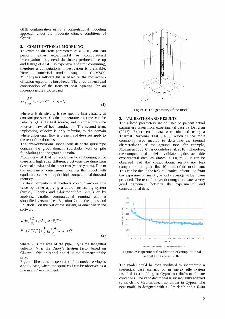
2

GHE configuration using a computational modeling

approach under the moderate climate conditions of

Cyprus.

2. COMPUTATIONAL MODELING

To examine different parameters of a GHE, one can

perform either experimental or computational

investigations. In general, the sheer experimental set-up

and testing of a GHE is expensive and time consuming,

therefore a computational investigation is preferable.

Here a numerical model using the COMSOL

Multiphysics software that is based on the convection-

diffusion equation is introduced. The three-dimensional

conservation of the transient heat equation for an

incompressible fluid is used:

p p

Tc c u T q Q

t

+ + =

(1)

where ρ is density, cp is the specific heat capacity at

constant pressure, T is the temperature, t is time, u is the

velocity, Q is the heat source, and q comes from the

Fourier’s law of heat conduction. The second term,

implicating velocity is only referring to the domain

where underwater flow is present and does not apply to

the rest of the domains.

The three-dimensional model consists of the spiral pipe

domain, the grout domain (borehole, well or pile

foundation) and the ground domain.

Modeling a GHE at full scale can be challenging since

there is a high scale difference between one dimension

(vertical z-axis) and the other two (x- and y-axes). Due to

the unbalanced dimensions, meshing the model with

equilateral cells will require high computational time and

memory.

Existent computational methods could overcome this

issue by either applying a coordinate scaling system

(Aresti, Florides and Christodoulides, 2016) or by

applying parallel computational running with a

simplified version (see Equation 2) on the pipes and

Equation 1 on the rest of the system, as emended in the

software:

( ) 21| |

2

p p t t

t t D

h

TAc Ac ue T

t

AAk T f u u Q

d

+ =

+ +

(2)

where A is the area of the pipe, uet is the tangential

velocity, fD is the Darcy’s friction factor based on

Churchill friction model and dh is the diameter of the

pipe.

Figure 1 illustrates the geometry of the model serving as

a study-case, where the spiral coil can be observed as a

line in a 3D environment.

Figure 1: The geometry of the model.

3. VALIDATION AND RESULTS

The related parameters are adjusted to present actual

parameters taken from experimental data by Dehghan

(2017). Experimental data were obtained using a

Thermal Response Test (TRT), which is the most

commonly used method to determine the thermal

characteristics of the ground (see, for example,

Mogensen 1983; Christodoulides et al. 2016). Therefore,

the computational model is validated against available

experimental data, as shown in Figure 2. It can be

observed that the computational results are less

compatible during the first 10 hours of the model run.

This can be due to the lack of detailed information from

the experimental results, as only average values were

provided. The rest of the graph though, indicates a very

good agreement between the experimental and

computational data.

Figure 2: Experimental validation of computational

model for a spiral GHE.

The model could be then modified to incorporate a

theoretical case scenario of an energy pile system

installed in a building in Cyprus for different climate

conditions. The validated model is subsequently adapted

to match the Mediterranean conditions in Cyprus. The

new model is designed with a 10m depth and a 0.4m

3

diameter. The selected model geometry (also seen in

Figure 1) consists of a 10m depth pile, a 6m depth spiral

coil, a 0.8m pile diameter and a 5m domain diameter. A

similar configuration is described at the new public

library in Limassol, Cyprus, where a spiral coil is

incorporated in a well. In order to obtain more accurate

and realistic results, ground temperature data were

considered, as in Figure 3, where it can be observed that

the temperature below a depth of 7m is constant at 22oC.

The same temperatures are observed in a similar case in

Limassol by Florides, Pouloupatis and Kalogirou (2011).

Figure 3: Recorder ground temperature at Lakatamia,

Cyprus for a day from each month of a year

(Pouloupatis, Florides and Tassou, 2011)

Figure 4: Recorded underground temperature at the

Lakatamia shallow zone (0–7m), shown is the best-fit

equation

Stylianou et al. (2019) have analyzed the data of Figure

3 and have illustrated a shallow zone temperature

gradient (Figure 4) to be used in the computational

model. The equation of the ground temperature is input

as initial temperature in the computational model. The

case of summer was examined for the month of July.

Furthermore, the ground characteristics of the case study

in Limassol are considered. The ground examined to

consist of marl, chalk and gravel, with the complete

model material properties described in Table 1.

Table 1: Material properties

Material k

Wm–1K–1

ρ

kg m–3

cp

J Kg–1 K–1

Description

Ground 1.4 2300 950 Marl, chalk

and gravel

Grout 1.628 2500 837 Reinforced

concrete

Pipes 0.42 1100 1465 HDPE

Water 0.6 998.2 4182 water

The configuration of the energy pile and the dimensional

characteristics are defined in Table 2.

Table 2: Model dimensional characteristics and

operating parameters

Dimensional Characteristics

Energy Pile length 10 m

Energy Pile diameter 0.8 m

Spiral coil diameter 32 mm

Pipe (coil) thickness 3 mm

Operating Parameters

Fluid flow rate 15 l/min

Inlet temperature 60 oC

Following the model set-up, the spiral pitch was varied

from 0.1m to 0.5m by 0.1m increments. With the spiral

pitch changed, the length of the pipe also changed since

the depth of the pile was kept the same. The results can

be seen in Figure 5.

Figure 5: Spiral pitch effect on outlet temperature at

different operating durations

The results obtained demonstrate that the higher the

pitch, the higher the outlet temperature of the pipe.

Similar results were obtained by Park et al. (2015) and

Park et al. (2016).

By investigating the higher operating time duration

(24h), it can be seen that the effect of the spiral pitch on

the outlet temperature is decreased. This is an expected

result since for long enough durations of the heat injected

48

48,5

49

49,5

50

0,1 0,2 0,3 0,4 0,5

Tem

per

atu

re [

deg

C]

pitch

Outlet temp 6h Outlet temp 12h Outlet temp 24h

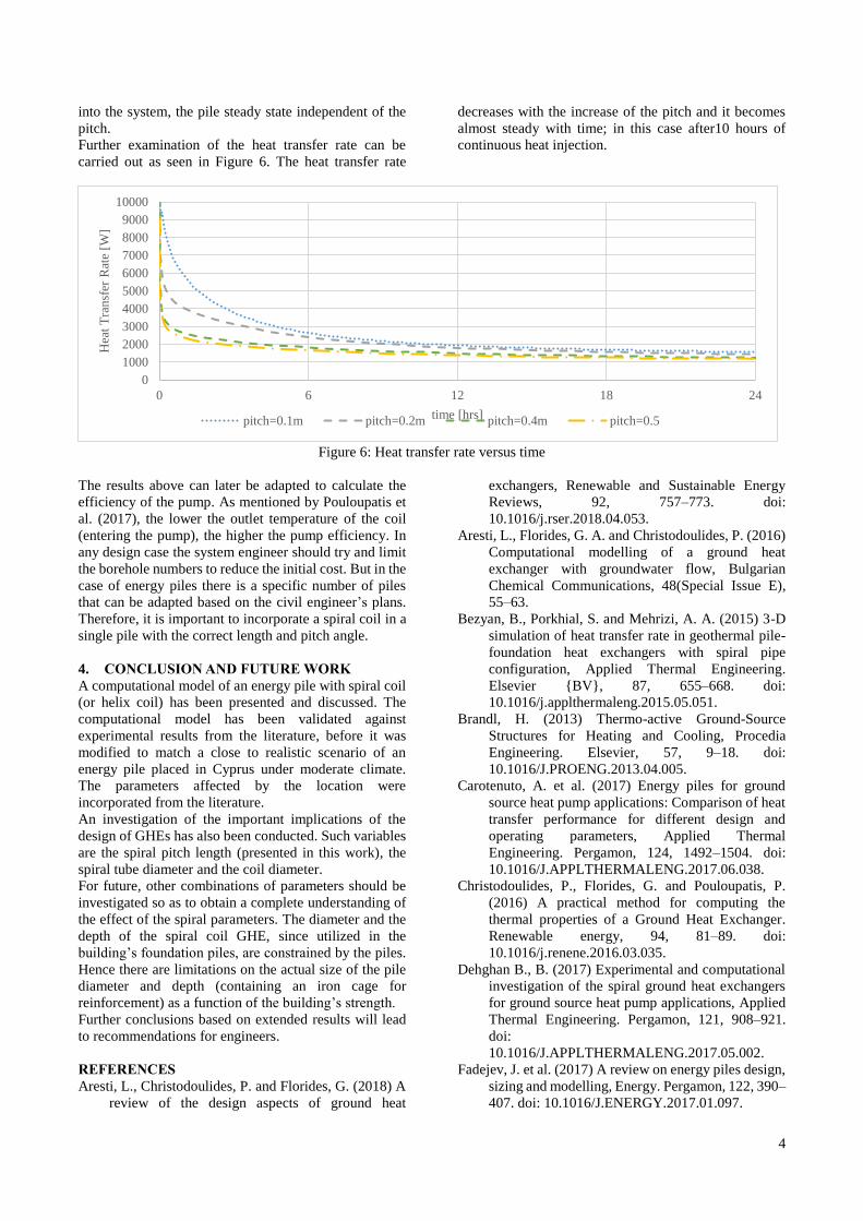
4

into the system, the pile steady state independent of the

pitch.

Further examination of the heat transfer rate can be

carried out as seen in Figure 6. The heat transfer rate

decreases with the increase of the pitch and it becomes

almost steady with time; in this case after10 hours of

continuous heat injection.

Figure 6: Heat transfer rate versus time

The results above can later be adapted to calculate the

efficiency of the pump. As mentioned by Pouloupatis et

al. (2017), the lower the outlet temperature of the coil

(entering the pump), the higher the pump efficiency. In

any design case the system engineer should try and limit

the borehole numbers to reduce the initial cost. But in the

case of energy piles there is a specific number of piles

that can be adapted based on the civil engineer’s plans.

Therefore, it is important to incorporate a spiral coil in a

single pile with the correct length and pitch angle.

4. CONCLUSION AND FUTURE WORK

A computational model of an energy pile with spiral coil

(or helix coil) has been presented and discussed. The

computational model has been validated against

experimental results from the literature, before it was

modified to match a close to realistic scenario of an

energy pile placed in Cyprus under moderate climate.

The parameters affected by the location were

incorporated from the literature.

An investigation of the important implications of the

design of GHEs has also been conducted. Such variables

are the spiral pitch length (presented in this work), the

spiral tube diameter and the coil diameter.

For future, other combinations of parameters should be

investigated so as to obtain a complete understanding of

the effect of the spiral parameters. The diameter and the

depth of the spiral coil GHE, since utilized in the

building’s foundation piles, are constrained by the piles.

Hence there are limitations on the actual size of the pile

diameter and depth (containing an iron cage for

reinforcement) as a function of the building’s strength.

Further conclusions based on extended results will lead

to recommendations for engineers.

REFERENCES

Aresti, L., Christodoulides, P. and Florides, G. (2018) A

review of the design aspects of ground heat

exchangers, Renewable and Sustainable Energy

Reviews, 92, 757–773. doi:

10.1016/j.rser.2018.04.053.

Aresti, L., Florides, G. A. and Christodoulides, P. (2016)

Computational modelling of a ground heat

exchanger with groundwater flow, Bulgarian

Chemical Communications, 48(Special Issue E),

55–63.

Bezyan, B., Porkhial, S. and Mehrizi, A. A. (2015) 3-D

simulation of heat transfer rate in geothermal pile-

foundation heat exchangers with spiral pipe

configuration, Applied Thermal Engineering.

Elsevier {BV}, 87, 655–668. doi:

10.1016/j.applthermaleng.2015.05.051.

Brandl, H. (2013) Thermo-active Ground-Source

Structures for Heating and Cooling, Procedia

Engineering. Elsevier, 57, 9–18. doi:

10.1016/J.PROENG.2013.04.005.

Carotenuto, A. et al. (2017) Energy piles for ground

source heat pump applications: Comparison of heat

transfer performance for different design and

operating parameters, Applied Thermal

Engineering. Pergamon, 124, 1492–1504. doi:

10.1016/J.APPLTHERMALENG.2017.06.038.

Christodoulides, P., Florides, G. and Pouloupatis, P.

(2016) A practical method for computing the

thermal properties of a Ground Heat Exchanger.

Renewable energy, 94, 81–89. doi:

10.1016/j.renene.2016.03.035.

Dehghan B., B. (2017) Experimental and computational

investigation of the spiral ground heat exchangers

for ground source heat pump applications, Applied

Thermal Engineering. Pergamon, 121, 908–921.

doi:

10.1016/J.APPLTHERMALENG.2017.05.002.

Fadejev, J. et al. (2017) A review on energy piles design,

sizing and modelling, Energy. Pergamon, 122, 390–

407. doi: 10.1016/J.ENERGY.2017.01.097.

0

1000

2000

3000

4000

5000

6000

7000

8000

9000

10000

0 6 12 18 24

Hea

t T

ran

sfer

Rat

e [W

]

time [hrs]pitch=0.1m pitch=0.2m pitch=0.4m pitch=0.5

5

Florides, G. A. et al. (2011) The geothermal

characteristics of the ground and the potential of

using ground coupled heat pumps in Cyprus,

Energy. Elsevier Ltd, 36(8), 5027–5036. doi:

10.1016/j.energy.2011.05.048.

Gao, J. et al. (2008) Numerical and experimental

assessment of thermal performance of vertical

energy piles: An application, Applied Energy.

Elsevier, 85(10), 901–910. doi:

10.1016/J.APENERGY.2008.02.010.

Gashti, E. H. N., Uotinen, V.-M. and Kujala, K. (2014)

Numerical modelling of thermal regimes in steel

energy pile foundations: A case study, Energy and

Buildings. Elsevier, 69, 165–174. doi:

10.1016/J.ENBUILD.2013.10.028.

de Moel, M. et al. (2010) Technological advances and

applications of geothermal energy pile foundations

and their feasibility in Australia, Renewable and

Sustainable Energy Reviews. Pergamon, 14(9),

2683–2696. doi: 10.1016/J.RSER.2010.07.027.

Mogensen, P. (1983) Fluid to duct wall heat transfer in

duct system heat storages. Document-Swedish

Council for Building Research, 16, 652–657.

Park, S. et al. (2015) Relative constructability and

thermal performance of cast-in-place concrete

energy pile: Coil-type GHEX (ground heat

exchanger), Energy, 81, 56–66. doi:

10.1016/j.energy.2014.08.012.

Park, S. et al. (2016) Influence of coil pitch on thermal

performance of coil-type cast-in-place energy piles,

Energy and Buildings. Elsevier, 129, 344–356. doi:

10.1016/J.ENBUILD.2016.08.005.

Pouloupatis, P. D. et al. (2017) Parametric analysis of the

factors affecting the efficiency of ground heat

exchangers and design application aspects in

Cyprus, Renewable Energy. Elsevier {BV}, 103,

721–728. doi: 10.1016/j.renene.2016.11.006.

Pouloupatis, P. D., Florides, G. and Tassou, S. (2011)

Measurements of ground temperatures in Cyprus

for ground thermal applications, Renewable

Energy. Elsevier {BV}, 36(2), 804–814. doi:

10.1016/j.renene.2010.07.029.

Stylianou I.I. et al., 2019. Modeling of Vertical Ground

Heat Exchangers in the Presence of Groundwater

Flow and Underground Temperature Gradient.

Energy and Buildings, 192, 15–30. doi:

10.1016/j.enbuild.2019.03.020

Suryatriyastuti, M. E., Mroueh, H. and Burlon, S. (2012)

Understanding the temperature-induced

mechanical behaviour of energy pile foundations,

Renewable and Sustainable Energy Reviews.

Pergamon, 16(5), 3344–3354. doi:

10.1016/J.RSER.2012.02.062.

Yoon, S. et al. (2015) Evaluation of the thermal

efficiency and a cost analysis of different types of

ground heat exchangers in energy piles, Energy

Conversion and Management. Pergamon, 105,

393–402. doi:

10.1016/J.ENCONMAN.2015.08.002.

Zhao, Q., Chen, B. and Liu, F. (2016) Study on the

thermal performance of several types of energy pile

ground heat exchangers: U-shaped, W-shaped and

spiral-shaped, Energy and Buildings. Elsevier

{BV}, 133, 335–344. doi:

10.1016/j.enbuild.2016.09.055.

GROUND SOURCE HEAT PUMPS COST ANALYSIS IN MODERATE CLIMATE

Lazaros Aresti(a), Paul Christodoulides(b), Vassilios Messaritis(c), Georgios A. Florides(d)

(a) Department of Electrical Engineering, Computer Engineering and Informatics, Cyprus University of Technology,

Limassol, Cyprus (b), (d) Faculty of Engineering and Technology, Cyprus University of Technology, Limassol, Cyprus

(c) Department of Mechanical Engineering and Materials Science and Engineering, Cyprus University of Technology,

Limassol, Cyprus

(a)lg.aresti@edu.cut.ac.cy, (b)paul.christodoulides@cut.ac.cy, (c)vassilios.messaritis@cut.ac.cy, (d)georgios.florides@cut.ac.cy

ABSTRACT

A debate is taken up on whether it is economically

preferential to install Ground Source Heat Pumps

(GSHPs), Renewable Energy Systems, instead of Air

Source Heat Pumps (ASHPs). To this end, a typical

house heating/cooling load for moderate climates is

chosen and the thermal response of Ground Heat

Exchangers (GHEs) of GSHPs and their characteristics

– based on experimental data and CFD-model

simulations in FlexPDE – are discussed. The results

indicate that with greater difference between the inlet

GSHP temperature water and the ground, a higher heat

rejection is observed. The GSHP capacity over the input

power operating temperature is affected by the fluid

temperature entering the Heat Pump, affecting the

system cost as more GHE boreholes may be needed for

reducing the temperature. A cost analysis is thus

presented for different-length GSHP systems and a

comparison of the total energy savings is obtained

versus highly competitive inverter technology ducted

series ASHP systems.

Keywords: Ground Source Heat Pump Systems, GHE

cost analysis in moderate climate conditions, Air Source

Heat Pumps

1. INTRODUCTION

Geothermal Energy, a form of Renewable energy, has

attracted attention in recent years due to the energy

shortage. While the transfer of heat from a high

temperature source to a low temperature one is natural,

the opposite is done through HPs that are commonly

used for the air-conditioning of buildings. A HP

operates with electricity, using as an exchange source

either the surrounding air (ASHPs) or water in the pipes

of a GHE (GSHPs) that uses the Earth’s energy to gain

or reject heat.

The GHEs, compared to air-to-air heat exchanger

systems, exhibit significantly higher performance (Yu et

al. 2013), but their installation cost is high, and they

require larger spaces. Recent research has focused on

the reduction of the cost (Aresti, Christodoulides and

Florides 2018) and, consequently, GSHP installations

that may be economically beneficial over convectional

heating and cooling systems have increased over the last

decade (Yang, Cui and Fang 2010). Naturally, there

have been studies in the literature concerned whether it

is cost beneficial to use GSHP instead of ASHPs.

Healy and Ugursal reported that between four different

residential heating/cooling systems in a residential

building in Nova Scotia, Canada, namely GSHP,

electric resistance heat, oil-fired furnace and ASHP

systems, the GSHP system was the least expensive to

install-operate (Healy and Ugursal, 1997).

For similar studies conducted in Turkey, the results

showed that the GSHP system is a cost-effective

solution compared to electric resistance, fuel oil, liquid

petrol gas, coal and diesel oil, with payback periods

between 8 and 21 years (Esen, Inalli and Esen 2006),

(Camdali and Tuncel 2013). Other studies include

Chang et al. in China with a payback period of 7.1 years

for a GSHP system versus a water-cooling machine and

matching gas furnace system (Chang et al. 2017), and

Badescu with a payback period of 3–10 years for a

GSHP system versus convectional systems and GHEs

with convectional systems (Badescu 2007).

On the other hand, Lu et al., using different economic

methods from previous studies, concluded GSHP

systems would provide an economic advantage

compared to the ASHP systems only in the long term

(40 years) (Lu et al., 2017).

In general, based on the literature, GSHP may or may

not be an economic solution for heating/cooling a

house, depending on many factors, such as ASHP

efficiency, location of the house and climate conditions

and installation cost of the GSHP (Christodoulides,

Aresti and Florides 2019). The work presented below

mainly aims at contributing in the study of the

effectiveness and usefulness of GSHP in moderate

climate conditions.

2. TYPICAL HOUSE LOAD AND MODERATE

CLIMATE DESIGN

To evaluate and compare the cost effectiveness of a

GSHP system, a typical house in moderate climate in

Cyprus is considered. The characteristics of the

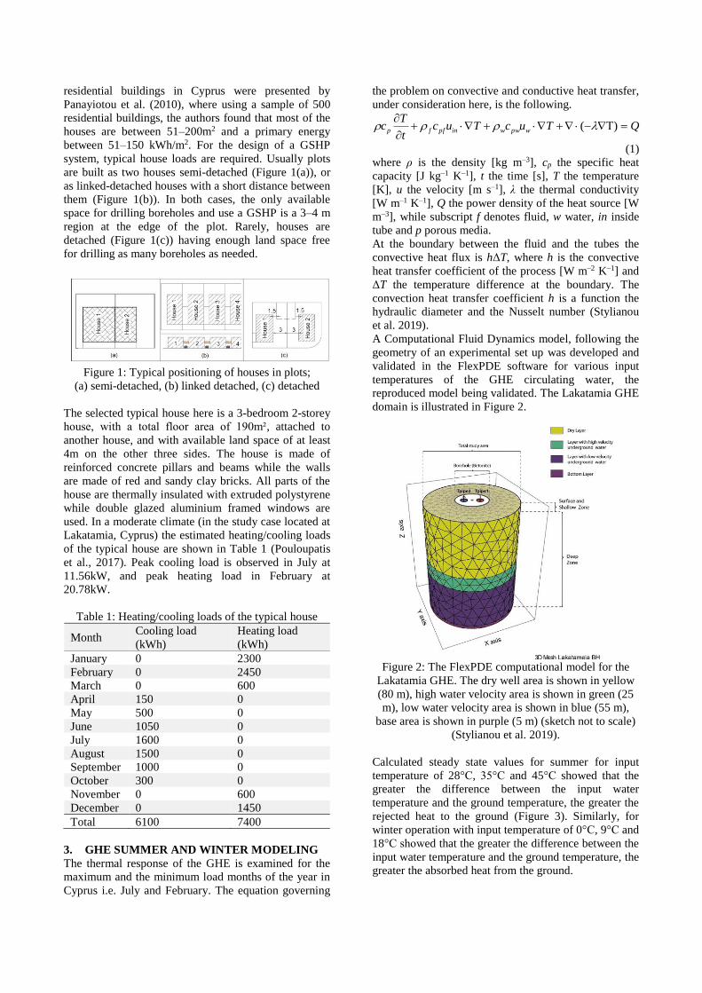
residential buildings in Cyprus were presented by

Panayiotou et al. (2010), where using a sample of 500

residential buildings, the authors found that most of the

houses are between 51–200m2 and a primary energy

between 51–150 kWh/m2. For the design of a GSHP

system, typical house loads are required. Usually plots

are built as two houses semi-detached (Figure 1(a)), or

as linked-detached houses with a short distance between

them (Figure 1(b)). In both cases, the only available

space for drilling boreholes and use a GSHP is a 3–4 m

region at the edge of the plot. Rarely, houses are

detached (Figure 1(c)) having enough land space free

for drilling as many boreholes as needed.

Figure 1: Typical positioning of houses in plots;

(a) semi-detached, (b) linked detached, (c) detached

The selected typical house here is a 3-bedroom 2-storey

house, with a total floor area of 190m², attached to

another house, and with available land space of at least

4m on the other three sides. The house is made of

reinforced concrete pillars and beams while the walls

are made of red and sandy clay bricks. All parts of the

house are thermally insulated with extruded polystyrene

while double glazed aluminium framed windows are

used. In a moderate climate (in the study case located at

Lakatamia, Cyprus) the estimated heating/cooling loads

of the typical house are shown in Table 1 (Pouloupatis

et al., 2017). Peak cooling load is observed in July at

11.56kW, and peak heating load in February at

20.78kW.

Table 1: Heating/cooling loads of the typical house

Month Cooling load

(kWh)

Heating load

(kWh)

January 0 2300

February 0 2450

March 0 600

April 150 0

May 500 0

June 1050 0

July 1600 0

August 1500 0

September 1000 0

October 300 0

November 0 600

December 0 1450

Total 6100 7400

3. GHE SUMMER AND WINTER MODELING

The thermal response of the GHE is examined for the

maximum and the minimum load months of the year in

Cyprus i.e. July and February. The equation governing

the problem on convective and conductive heat transfer,

under consideration here, is the following.

QTucTuct

Tc wpwwinpffp =−+++

)(

(1)

where ρ is the density [kg m–3], cp the specific heat

capacity [J kg–1 K–1], t the time [s], T the temperature

[K], u the velocity [m s–1], λ the thermal conductivity

[W m–1 K–1], Q the power density of the heat source [W

m–3], while subscript f denotes fluid, w water, in inside

tube and p porous media.

At the boundary between the fluid and the tubes the

convective heat flux is hΔT, where h is the convective

heat transfer coefficient of the process [W m–2 K–1] and

ΔT the temperature difference at the boundary. The

convection heat transfer coefficient h is a function the

hydraulic diameter and the Nusselt number (Stylianou

et al. 2019).

A Computational Fluid Dynamics model, following the

geometry of an experimental set up was developed and

validated in the FlexPDE software for various input

temperatures of the GHE circulating water, the

reproduced model being validated. The Lakatamia GHE

domain is illustrated in Figure 2.

Figure 2: The FlexPDE computational model for the

Lakatamia GHE. The dry well area is shown in yellow

(80 m), high water velocity area is shown in green (25

m), low water velocity area is shown in blue (55 m),

base area is shown in purple (5 m) (sketch not to scale)

(Stylianou et al. 2019).

Calculated steady state values for summer for input

temperature of 28°C, 35°C and 45°C showed that the

greater the difference between the input water

temperature and the ground temperature, the greater the

rejected heat to the ground (Figure 3). Similarly, for

winter operation with input temperature of 0°C, 9°C and

18°C showed that the greater the difference between the

input water temperature and the ground temperature, the

greater the absorbed heat from the ground.

Figure 3: GHE exiting fluid temperature plotted against

time for three cases of steady temperature fluid entering

the GHE of 45, 35 and 28 °C (Stylianou et al. 2019).

The characteristics of such GHE/GSHP are given in

Pouloupatis et al. (2017). The HP capacity over the

input power is nearly doubled from a HP entering fluid

temperature of 44°C to 20°C (cooling) (similarly for

heating). This means that to achieve lower temperatures

a bigger number of boreholes are needed and

consequently the greater the initial cost will be.

Therefore, the designer should consider the benefits of a

greater HP efficiency against the disadvantage of

greater initial cost.

4. GHE COST ANALYSIS

Robert and Gosselin demonstrated a good case of a

techno-economic analysis of a GSHP system (Robert

and Gosselin 2014). The total cost of any GSHP system

consists of the initial capital invested and the operating

costs, namely the sum of costs of the HP, mechanical

room installation, drilling, piping, ground loop

installation, fittings, etc., electricity consumption by the

HP, the heat transfer fluid circulation pump and the

backup heating/cooling system.

Hence, the difference in the cost between an ASHP and

a GSHP system lays in the GHE and the associated

equipment, such as the borehole extraction, U-tube

GHE, grout material, ground loop installation, header-

flowmeter valves, horizontal pipe circuits, and some

general expenses (Christodoulides, Aresti and Florides

2019). Typical extra costs for the installation of a GHE

of 400m, 600m and 800m are calculated at €12600,

€18200 and €23800 respectively, based on information

taken from companies based in Cyprus in 2018.

Note that, as stated by Rawlings and Sykulski, direct

comparison between different countries or even regions

cannot be done owing to economies of scale (Rawlings

and Sykulski 1999).

Now, a specifically designed inverter technology ducted

series ASHP of similar capacity, can have a ratio of

Pump Capacity/Power Input of around 3.0 (cooling) and

3.7 (heating). An estimation for the electrical power

needed to cover the total heating/cooling load per year

is shown in Table 2.

Lu et al. discussed different methods used in the

literature to examine the economic benefits of installing

a GSHP system (Lu et al. 2017). It is though beyond the

scope of the current study to go in detail into such

methods, as the goal of comparing a single GSHP (of a

vertical GHE) and a simple ASHP can be achieved

through a simple methodology explained below with

adequate precision.

The power savings per year for (a) the 800m GHE are

961 kWh, (b) the 600m GHE are 862 kWh and (c) the

400m GHE are 673 kWh. Considering the current price

for house holdings of 0.19€/kWh would result to the

following corresponding savings per year: (a) €183, (b)

€164, and (c) €128. It turns out that, for all cases, the

payback period would be well over 20 years.

The results show that the new specifically designed,

inverter type ASHPs, have reached such a high stage of

technology that can antagonize strongly GSHPs for

residential use.

Table 2: Energy savings per year for the typical house

Season /GHE

length /Ratio

Cooling/

Heating

load

(kWh)

Input

electrical

energy

(kWh)

Savings

vs ASHP

(kWh)

ASHP summer

/3.0 6100 2033

ASHP winter

/3.7 7400 2000

GSHP summer

/800m /4.9 6100 1245 788

GSHP summer

/600m /4.7 6100 1298 735

GSHP summer

/400m /4.4 6100 1386 647

GSHP winter

/800m /4.05 7400 1827 173

GSHP winter

/600m /3.95 7400 1873 127

GSHP winter

/400m /3.75 7400 1973 27

5. CONCLUSION

The work presented here has pointed to novelty with its

study of a typical house in Cyprus (moderate climate)

with a GSHP system, through the analysis of its thermal

response numerically. A typical residential building in

Cyprus has been presented with heating/cooling loads in

moderate Mediterranean climate conditions. The 3-

bedroom house of 190m2 has peak cooling/heating

loads of 11.56 kW and 20.78 kW.

Moreover, the paper has offered a cost analysis of a

GSHP system with different lengths as well as a cost

comparison of GSHP systems with an ASHP system

based on experimental data. It turned out that the

payback period of using GSHP systems over ASHPs

would be well over 20 years, making it not an

economical solution in the specific case. This is due to

comparable Pump Capacity/Power Input ratios between

specifically designed inverted technology ducted series

ASHPs and GSHPs.

Even using methods such as Present Worth, Annual

Worth, Internal Rate of Return, External Rate of Return,

Simple Payback Period, Discounted Payback Period

would not alter dramatically the result (Lu et al., 2017),

(Christodoulides, Aresti and Florides 2019).

Concluding, one could argue that GSHPs would be an

economic and viable solution as alternatives to ASHPs

if sufficiently subsidized as Renewable energy source

by the State.

REFERENCES

Aresti L., Christodoulides P. and Florides G., 2018. A

review of the design aspects of ground heat

exchangers. Renewable and Sustainable Energy

Reviews, 92, pp. 757–773.

Badescu V., 2007. Economic aspects of using ground

thermal energy for passive house heating.

Renewable Energy, 32(6), pp. 895–903.

Camdali U. and Tuncel E., 2013. An economic analysis

of horizontal Ground Source Heat Pumps

(GSHPs) for use in heating and cooling in Bolu,

Turkey. Energy Sources, Part B: Economics,

Planning and Policy, 8(3), pp. 290–303.

Chang J. et al., 2017. The applications and economic

analysis of Ground Source Heat Pump (GSHP) in

certain national games sports centre. Procedia

Engineering, 205, pp. 863–870.

Christodoulides P., Aresti L. and Florides G., 2019. Air-

conditioning of a typical house in moderate

climates with Ground Source Heat Pumps and

cost comparison with Air Source Heat Pumps.

Applied Thermal Engineering, p. 113772.

Esen H., Inalli M. and Esen M., 2006. Technoeconomic

appraisal of a ground source heat pump system for

a heating season in eastern Turkey. Energy

Conversion and Management, 47(9–10), pp.

1281–1297.

Healy P.F. and Ugursal V.I., 1997. Performance and

economic feasibility of ground source heat pumps

in cold climate. International Journal of Energy

Research, 21(10), pp. 857–870.

Lu Q. et al., 2017. Economic analysis of vertical ground

source heat pump systems in Melbourne. Energy,

125, pp. 107–117.

Panayiotou G.P. et al., 2010. The characteristics and the

energy behaviour of the residential building stock

of Cyprus in view of Directive 2002/91/EC.

Energy and Buildings, 42(11), pp. 2083–2089.

Pouloupatis P.D. et al., 2017. Parametric analysis of the

factors affecting the efficiency of ground heat

exchangers and design application aspects in

Cyprus. Renewable Energy, 103, pp. 721–728.

Rawlings R.H.D., 1999. Ground source heat pumps: A

technology review. Building Services Engineering

Research and Technology, 20(3), pp. 119–129.

Robert F. and Gosselin L., 2014. New methodology to

design ground coupled heat pump systems based

on total cost minimization. Applied Thermal

Engineering, 62(2), pp. 481–491.

Stylianou I.I. et al., 2019. Modeling of Vertical Ground

Heat Exchangers in the Presence of Groundwater

Flow and Underground Temperature Gradient.

Energy and Buildings, 192, pp. 15-30.

Yang H., Cui P. and Fang Z., 2010. Vertical-borehole

ground-coupled heat pumps: A review of models

and systems. Applied Energy, 87(1), pp. 16–27.

Yu X. et al., 2013. Thermal response test and numerical

analysis based on two models for ground-source

heat pump system. Energy and Buildings, 66, pp.

657–666.

SCHEDULING MULTIPLE LIFT VEHICLES IN A COMMON SHAFT IN AUTOMATED VEHICLE STORAGE AND RETRIEVAL SYSTEMS

Andreas Habl(a), Vincent Balducci(b), Johannes Fottner(c)

(a),(b),(c) Chair of Materials Handling, Material Flow, Logistics

Technical University of Munich, Germany

(a)andreas.habl@tum.de, (b)vincent.balducci@tum.de, (c)j.fottner@tum.de

ABSTRACT Automated vehicle storage and retrieval systems (AVSRSs) provide an efficient and powerful way to store small unit loads. In order to meet the increasing requirements in terms of the flexibility and throughput capacity of these systems, a new type of high-powered AVSRS can be deployed. In high-powered AVSRSs, multiple lift vehicles move in one common shaft instead of just a single vehicle, so as to further increase the throughput capacity of lifting systems and the vertical transport. In this work, we present and compare different scheduling algorithms that allow for the robust and efficient control of multiple lift vehicles. By performing simulation experiments, we show that the throughput capacity of lifting systems can be increased significantly. Keywords: automated vehicle storage and retrieval systems, shuttle systems, discrete-event simulation, scheduling

1. INTRODUCTION For the realization of scalable and efficient warehouses, automated vehicle storage and retrieval systems (AVSRSs) are being increasingly deployed. AVSRSs, also known as shuttle systems, are used for storing small transportation units (TUs) in order to supply picking or manufacturing areas on the basis of the goods-to-person principle. A key concept of this technology is the separation of horizontal and vertical transportation, executed by shuttle and lift vehicles, respectively. (FEM 2017) There are different configurations of AVSRSs which have evolved over time, the most common and powerful configuration being characterized by shuttle vehicles restricted to a single storage aisle and tier (Lienert and Fottner 2017). At each tier, a shuttle vehicle transports TUs in a horizontal direction from and to the storage locations. In this type of AVSRS, a number of lifting systems, each with a vertically operating lift vehicle, enable vertical movement of TUs from and to the tiers. As lifting systems often limit the throughput capacity of AVSRSs (Lerher et al. 2015), more than one lift vehicle could be deployed in these systems (see figure 1). As a consequence, the overall throughput capacity of AVSRSs could be increased by adding more lift vehicles

to the lifting systems. In this way, the throughput capacity of already existing AVSRSs could be increased as well, and thus transformed into high-powered AVSRSs.

Figure 1: Several lift vehicles moving in a common shaft in an aisle of a high-powered AVSRS The remainder of the paper is organized as follows. In the second section, a literature review of the respective areas is presented. In section 3, a description of the algorithms developed for scheduling multiple lift vehicles is given. In section 4, the simulation model as well as the model validation is described. In section 5, the simulation results of the different scheduling algorithms are presented. Finally, section 6 provides a conclusion and outlook. 2. LITERATURE REVIEW In the following section, we give a review of related work in the field of throughput analysis and of the control algorithms of AVSRSs. Finally, we present existing scheduling problems in other applications. 2.1. Throughput Analysis of Automated Vehicle

Storage and Retrieval Systems When it comes to the dimensioning of AVSRSs, the throughput analysis of these systems is of high relevance. In order to determine the throughput of AVSRS, two fundamental approaches exist. Analytical models, e.g. based on queuing theory (Marchet et al. 2012; Eder and

Kartnig 2016), can be used to analyze the performance of less complex systems. However, especially when a variety of configurations or complex systems have to be investigated, throughput analysis is generally performed by using simulation. Lerher et al. (2015) conduct a simulation study in order to analyze the effect of different parameters on throughput. Zhao et al. (2016) present a simulation model for investigating various rack configurations with multiple lifting systems, in order to identify the ideal configuration in a short space of time. 2.2. Control Algorithms of Automated Vehicle

Storage and Retrieval Systems Controlling strategies in conventional AVSRSs are often limited to simple priority rules, since the transport processes do not require sophisticated algorithms. However, when deploying high-powered AVSRSs with multiple lift vehicles operating in a common shaft and lifting system as well as multiple shuttle vehicles moving along the same rail, scheduling algorithms need to be applied in order to prevent collisions and to ensure efficient transport processes. By introducing the shuttle-vehicle scheduling problem, Habl et al. (2019) present a control algorithm to schedule multiple shuttle vehicles moving on a common rail. In line with this, the lift-vehicle scheduling problem occurs in lifting systems of high-powered AVSRSs. The paper most closely related to the lift-vehicle scheduling problem is presented in (Carlo and Vis 2012), with the scheduling of two non-passing lift vehicles mounted along a common shaft. This was enhanced in (Zhao et al. 2018) by considering the acceleration and deceleration of the lift vehicles. However, the number of lift vehicles was limited to two vehicles, whereas in high-powered AVSRSs there can be more than two lift vehicles moving in a common shaft and lifting system. 2.3. Scheduling Algorithms in Other Applications In order to prevent collisions between and blockings of the vehicles, efficient strategies for scheduling the transportation tasks need to be applied to each lifting system. However, we can find similar scheduling problems with non-crossing constraints in other logistics applications, for example port cranes, factory cranes, elevators, and industrial robots. Kress et al. (2019) present a dynamic programming algorithm and a related beam search heuristic to schedule two gantry cranes moving along one rail while avoiding interferences. Peterson et al. (2014) present a heuristic algorithm to schedule several factory cranes on a common track by using a block-sequencing method. Takahashi et al. (2003) present an optimized zoning strategy for controlling two elevator cars in one shaft by using a genetic algorithm to determine optimal zoning. Erdoğan et al. (2014) present exact and heuristic algorithms to schedule two robots operating on a common line. In this work, we leverage these existing concepts in order to address the lift vehicle scheduling problem described

above. In doing so, we develop and apply three scheduling algorithms in order to control multiple lift vehicles in a common shaft. Since we consider different configurations of lifting systems, we evaluate the performance and robustness of the developed scheduling algorithms by using the simulation-based approach. 3. SCHEDULING ALGORITHMS When deploying multiple lift vehicles in a common shaft, the vehicles need to be coordinated in order to prevent blockages and collisions between them, and to minimize empty driving times and waiting times. In this section, we present the control algorithms for the robust and efficient scheduling of multiple lift vehicles. 3.1. Rigid and Rolling Block-sequencing Algorithm Our first approach towards scheduling multiple lift vehicles with non-crossing constraints relies on the algorithm for scheduling several factory cranes on a common track by using a rigid block-sequencing method, as presented in (Peterson et al. 2014). The algorithm was already adapted in (Habl et al. 2019) to shuttle vehicles which perform horizontal transportations in high-powered AVSRSs, and further improved in (Habl et al. 2019) so as to apply the algorithm in multi-deep storage. In this work, the algorithm is adapted to lift vehicles for optimizing vertical transport in high-powered AVSRSs. The algorithm successively extracts a selected number of jobs from the job list for processing and creates a decision tree of possible states (partial and complete schedules). Thereafter, the extracted jobs are assigned to the lift vehicles according to the selected schedule with the lowest completion time. Due to the exponential growth of the decision tree, the algorithm’s computation time is reduced by the heuristic developed in (Peterson et al. 2014). This includes the pruning of inferior partial schedules (dominance check) as well as chopping partial schedules when the heuristic threshold is passed. However, since every block of jobs needs to be fully completed by the vehicles, it emerges that some of the faster vehicles are subject to waiting times. In order to further optimize this scheduling process, we combine rolling scheduling to the block-sequencing method to obtain a more dynamic version of the existing algorithm. This means that instead of starting the next block iteration after the last job of the block has been finished, new jobs are added to the schedule when the first vehicle has completed its jobs (see figure 2). 3.2. Cluster-sequencing Algorithm The second approach for scheduling multiple lift vehicles in a common shaft is based on the algorithm for controlling multiple stacker cranes on a common rail, as given in (Kung et al. 2014). The algorithm combines several transport jobs into a cluster and uses dynamic programming to obtain the optimum sequence. The size of a cluster corresponds to the number of vehicles.

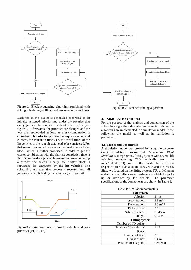
Start

Scheduled jobs = total number of jobs?

Schedule next block of jobs

Add block of jobs to scheduled jobs

Execute block of jobs

Execute last block of jobs

yes

End

Lift vehicle has completed all its assigned jobs?

no

yesno

Determine block size

Figure 2: Block-sequencing algorithm combined with rolling scheduling (rolling block-sequencing algorithm)

Each job in the cluster is scheduled according to an initially assigned priority and under the premise that every job can be executed without interruption (see figure 3). Afterwards, the priorities are changed and the jobs are rescheduled as long as every combination is considered. In order to optimize the sequence of several clusters, the transition times, i.e. the travel times of the lift vehicles to the next cluster, need to be considered. For that reason, several clusters are combined into a cluster block, which is further processed. In order to get the cluster combination with the shortest completion time, a list of combinations (states) is created and searched using a breadth-first search. Finally, the cluster block is forwarded for execution by the lift vehicles. The scheduling and execution process is repeated until all jobs are accomplished by the vehicles (see figure 4).

Figure 3: Cluster version with three lift vehicles and three priorities (P1, P2, P3)

Start

Scheduled clusters = number of jobs / number of

vehicles?

Schedule next cluster block

Execute jobs in cluster block

Add cluster block to scheduled clusters

Schedule and execute remaining jobs

yes

End

no

Determine cluster block

Figure 4: Cluster-sequencing algorithm

4. SIMULATION MODEL For the purpose of the analysis and comparison of the scheduling algorithms described in the section above, the algorithms are implemented in a simulation model. In the following, the model as well as its validation is presented. 4.1. Model and Parameters A simulation model was created by using the discrete-event simulation environment Tecnomatix Plant Simulation. It represents a lifting system with several lift vehicles, transporting TUs vertically from the input/output (I/O) point to the transfer buffer of the respective tier of an aisle in an AVSRS and vice versa. Since we focused on the lifting system, TUs at I/O point and at transfer buffers are immediately available for pick-up or drop-off by the vehicle. The parameter specifications of the components are shown in Table 1.

Table 1: Simulation parameters Lift vehicle Velocity 2 m/s

Acceleration 2.5 m/s² Deceleration 2.5 m/s² Pick-up time 2.5 s

Safety distance 0.045 m Height 0.35 m

Lifting system Number of I/O points 1

Number of lift vehicles 1 - 6 Rack

Number of tiers 30 Height of tier 0.4 m

Position of I/O point Centered

In order to test and compare the developed scheduling algorithms in different scenarios, a series of simulation experiments is performed. In each simulation experiment, a list of transport jobs (storage and retrieval) for the lifting system is generated after system initialization, and scheduled for the lift vehicles. After completion of all jobs the throughput capacity of the system is calculated by measuring the time needed for fulfilment. 4.2. Model Validation Since storage and retrieval locations (tiers) are determined randomly during job generation, the number of replications of the simulation experiments as well as the number of transport jobs need to be adjusted accordingly, in order to reduce the luck factor. In a preliminary study, we varied the number of replications of a reference experiment from 10 to 1000 replications. In order to determine the throughput of the reference experiment, a simulation with one lift vehicle in a lifting system which is serving 30 tiers with a centered I/O point is conducted. The number of transport jobs is varied from 5 to 5000 jobs in this experiment (see figure 5).

Figure 5: Variation of throughput depending on number of jobs when performing 40 replications With 40 replications and 500 jobs in each experiment, we obtain a mean value of 400 jobs per hour and a standard deviation of 3.6 jobs per hour, which leads to a 95 % confidence interval of 400 ± 1 job per hour. Since this is considered “sufficient” in this study, this parameter set is used for the following analysis. As already described in section 3, the computation time of the block-sequencing algorithm is reduced by a heuristic, including chopping partial schedules when the heuristic threshold is passed. In the following analysis, the threshold is set to 300 states and the number of deleted states is set to 30 % of the threshold. 5. SIMULATION RESULTS In this section, we present and discuss the results of the conducted simulation study on the basis of the simulation model described in the section above. Figure 6-8 show the improved throughput capacity of the lifting system by deploying up to six lift vehicles and by

applying the scheduling algorithms rigid block-sequencing, rolling block-sequencing, and cluster-sequencing. The obtained throughput when deploying only one vehicle is selected as a reference. Essentially, the throughput capacity of a lifting system can be increased by deploying additional lift vehicles. However, the largest relative increase can be achieved by adding one more vehicle to the system. Since only one I/O point is available in the considered lifting system, other vehicles interfere with each other and as a result, throughput capacity increases to a lesser extent. As can be seen in figure 6, the throughput capacity can be improved by 46 % when deploying two vehicles and by applying the cluster-sequencing algorithm to the lifting system. By adding up to six vehicles to the lifting system, the throughput capacity increases by up to 88 %.

Figure 6: Increase of throughput depending on the number of vehicles by applying cluster-sequencing algorithm (cluster block size of 20 jobs)

Figure 7 shows that by applying the rigid block-sequencing algorithm, throughput capacity can be improved by 61 % when deploying two vehicles and by up to 83 % when deploying four vehicles. However, the throughput capacity decreases when deploying more than four vehicles. An increasing number of vehicles increases the solution space, thus it increases the probability that the applied heuristic in the algorithm excludes the optimum solution.

Figure 7: Increase of throughput depending on the number of vehicles by applying rigid block-sequencing algorithm (block size of five jobs) Similarly, when applying the rolling block-sequencing algorithm, throughput capacity can be improved by 68 % when deploying two vehicles and by up to 92 % when deploying four vehicles (see figure 8).

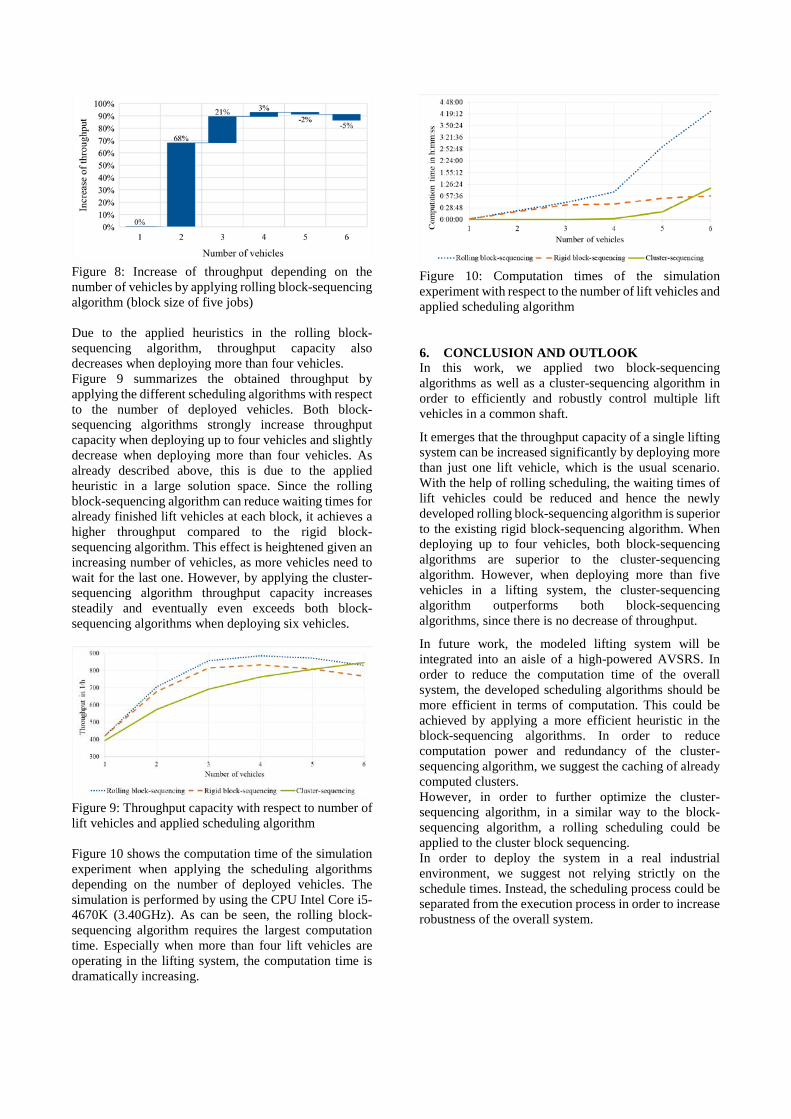
Figure 8: Increase of throughput depending on the number of vehicles by applying rolling block-sequencing algorithm (block size of five jobs)

Due to the applied heuristics in the rolling block-sequencing algorithm, throughput capacity also decreases when deploying more than four vehicles. Figure 9 summarizes the obtained throughput by applying the different scheduling algorithms with respect to the number of deployed vehicles. Both block-sequencing algorithms strongly increase throughput capacity when deploying up to four vehicles and slightly decrease when deploying more than four vehicles. As already described above, this is due to the applied heuristic in a large solution space. Since the rolling block-sequencing algorithm can reduce waiting times for already finished lift vehicles at each block, it achieves a higher throughput compared to the rigid block-sequencing algorithm. This effect is heightened given an increasing number of vehicles, as more vehicles need to wait for the last one. However, by applying the cluster-sequencing algorithm throughput capacity increases steadily and eventually even exceeds both block-sequencing algorithms when deploying six vehicles.

Figure 9: Throughput capacity with respect to number of lift vehicles and applied scheduling algorithm Figure 10 shows the computation time of the simulation experiment when applying the scheduling algorithms depending on the number of deployed vehicles. The simulation is performed by using the CPU Intel Core i5-4670K (3.40GHz). As can be seen, the rolling block-sequencing algorithm requires the largest computation time. Especially when more than four lift vehicles are operating in the lifting system, the computation time is dramatically increasing.

Figure 10: Computation times of the simulation experiment with respect to the number of lift vehicles and applied scheduling algorithm 6. CONCLUSION AND OUTLOOK In this work, we applied two block-sequencing algorithms as well as a cluster-sequencing algorithm in order to efficiently and robustly control multiple lift vehicles in a common shaft.

It emerges that the throughput capacity of a single lifting system can be increased significantly by deploying more than just one lift vehicle, which is the usual scenario. With the help of rolling scheduling, the waiting times of lift vehicles could be reduced and hence the newly developed rolling block-sequencing algorithm is superior to the existing rigid block-sequencing algorithm. When deploying up to four vehicles, both block-sequencing algorithms are superior to the cluster-sequencing algorithm. However, when deploying more than five vehicles in a lifting system, the cluster-sequencing algorithm outperforms both block-sequencing algorithms, since there is no decrease of throughput.

In future work, the modeled lifting system will be integrated into an aisle of a high-powered AVSRS. In order to reduce the computation time of the overall system, the developed scheduling algorithms should be more efficient in terms of computation. This could be achieved by applying a more efficient heuristic in the block-sequencing algorithms. In order to reduce computation power and redundancy of the cluster-sequencing algorithm, we suggest the caching of already computed clusters. However, in order to further optimize the cluster-sequencing algorithm, in a similar way to the block-sequencing algorithm, a rolling scheduling could be applied to the cluster block sequencing. In order to deploy the system in a real industrial environment, we suggest not relying strictly on the schedule times. Instead, the scheduling process could be separated from the execution process in order to increase robustness of the overall system.

REFERENCES Carlo H. J. and Vis I. F.A., 2012. "Sequencing dynamic

storage systems with multiple lifts and shuttles." International Journal of Production Economics 140:844–853.

Eder M. and Kartnig G., 2016. "Throughput analysis of S/R shuttle systems and ideal geometry for high performance." FME Transaction 44:174–179.

Erdoğan G., Battarra M. and Laporte G., 2014. "Scheduling twin robots on a line." Naval Research Logistics (NRL) 61:119–130.

FEM European materials handling federation, 2017. Guideline Cycle time calculation for automated vehicle storage and retrieval systems Last modfied 08.2017.

Habl A., Lienert T., Pradines G. and Fottner J., 2019. "Vehicle Coordination and Configuration in high-powered Automated Vehicle Storage and Retrieval Systems." 18. ASIM-Fachtagung Simulation in Produktion und Logistik, Chemnitz (Submitted).

Habl A., Plapp V. and Fottner J., 2019. "Operating high-powered Automated Vehicle Storage and Retrieval Systems in multi-deep Storage." 9th International Conference on Logistics, Informatics and Service Sciences (Submitted).

Kress D., Dornseifer J. and Jaehn F., 2019. "An exact solution approach for scheduling cooperative gantry cranes." European Journal of Operational Research 273:82–101.

Kung Y., Kobayashi Y., Higashi T., Sugi M. and Ota J., 2014. "Order scheduling of multiple stacker cranes on common rails in an automated storage/retrieval system." International Journal of Production Research 52:1171–1187.

Lerher T., Ekren Y. B. and Sari Z., 2015. "Simulation Analysis of Shuttle Based Storage and Retrieval Systems." International Journal of Simulation Modelling:48–59.

Lienert T. and Fottner J., 2017. "No More Deadlocks – Applying The Time Window Routing Method To Shuttle Systems." 169–175.

Marchet G., Melacini M., Perotti S. and Tappia E., 2012. "Analytical model to estimate performances of autonomous vehicle storage and retrieval systems for product totes." International Journal of Production Research 50:7134–7148.

Peterson B., Harjunkoski I., Hoda S. and Hooker, J. N., 2014. "Scheduling multiple factory cranes on a common track." Computers & Operations Research 48:102–112.

Takahashi S., Kita H., Suzuki H., Sudo T. and Markon S., 2003. "Simulation-based optimization of a controller for multi-car elevators using a genetic algorithm for noisy fitness function." In The 2003 Congress on Evolutionary Computation, 2003. CEC '03, 1582–1587: IEEE.

Zhao N., Luo L. and Lodewijks G., 2018. "Scheduling two lifts on a common rail considering acceleration and deceleration in a shuttle based storage and

retrieval system." Computers & Industrial Engineering 124:48–57.

Zhao N., Luo L., Zhang S. and Lodewijks G., 2016. "An efficient simulation model for rack design in multi-elevator shuttle-based storage and retrieval system." Simulation Modelling Practice and Theory 67:100–116.

SIMULATION OF HUMAN PIONEERING ON MARS

Bonato M. J. D.(a), Carneiro A. B. (b), Fadel L. M. A.(c), Koga R. Y.(d), Rodrigues A. L. B. V. (e), Silva J. L. A.(f),

Teixeira T. M.(g), Todesco G. (h)

FACENS - Sorocaba Engineering College

Rodovia Senador José Ermírio de Moraes, 1425 - Sorocaba - São Paulo - Brazil

mauriciojandir@gmail.com(a), andre.carneiro@facens.br (b), fadellorene@gmail.com(c), rafa_yumi99@hotmail.com(d),

andrea.braga@facens.br(e), jose-lucassilva@hotmail.com(f), thamoreira@icloud.com(g), glauco.todesco@facens.br (h)

ABSTRACT

This paper shows the work developed on the NASA

SIMULATION EXPLORATION EXPERIENCE 2019

(SEE 2019) by Faculty of Engineering of Sorocaba

(FACENS) team. The SEE is a project based on three-

dimensional modeling that involved fourteen teams from

ten different countries with the objective of simulating a

virtual mission using Distributed Observation Network

(DON) and High-Level Architecture (HLA). FACENS

team was responsible for developing a mars habitat,

containig astronauts and resources that enable astronauts

life’s during missions.

In this work, seven simulations were developed: two

rovers, one excavation mine, one oxygen factory, one

mars habitat, one cargo transport and the astronaut.

In order to create this simulation, several surveys were

carried out in order to simulate an environment as close

as possible to the real one. Being investigated the

constitution of soil and atmosphere, acceleration of

gravity, pressure, climate, among other similar items.

The simulation used JAVA language and three-

dimensional modeling in softwares like Blender,

SketchUp and 3DS max, in order to facilitate the

visualization of what is being simulated in real time.

Keywords: astronaut, DON, HLA, mars habitat, SEE,

simulation.

1. INTRODUCTION

The Simulation Exploration Experience (SEE) is an

international modeling and simulation (M&S) project

created by National Aeronautics and Space

Administration (NASA) to integrate various educational

institutions around the world. At the beginning of every

SEE project, NASA proposes to the member institutions

a space mission, which specifies how the environment is

and what can be done during the project, which must be

fulfilled through cooperation among the participating

teams, being each team responsible for the creation of its

own part of the simulation.

Since 2015 FACENS team have participated in the SEE.

In 2015 was realized a system to capture asteroids. In

2017, FACENS team was responsible for the modeling

and simulation of a functional lunar habitat, with all

essential subsystems, as well as for creating an astronaut

model. In 2018 was developed a life-support system in

Mars, it was developed four simulations: one rover to

find water, a second rover to collect hydrated salts from

an excavation mine, one oxygen plant responsible for

removing water from the salts and one excavation mine.

In this year the focus of our mission in the SEE 2019 was

expanded to human colonization on Mars, thus part of the

mission was using the four simulations developed on

SEE 2018 and making a more complex one by adding

three simulations that involves the development of the

astronaut’s accommodation and the resources that

enables theirs life during missions. Thus was developed

a mars habitat, codename HOME, capable of housing

astronauts on long-duration mars missions, a cargo

transportation, codename SPEL and the astronaut,

codename MANS.

The habitat was designed and developed having in mind

many aspects and meeting the necessary requirements to

provide survival and living conditions, as well as safety

and comfort. The HOME has different areas and

environments and it was designed to be replicated and

expanded. The cargo transportation was designed to

transport loads in the surface of Mars.

2. SEE MISSION 2019

The 2019 NASA’s mission was to create a Mars colony,

a base for future exploration missions. Continuing and

expanding the project developed in SEE 2018, making a

simulation more complex in architecture, with the

creation of a colony on Mars, as a basis for future

exploration missions linked to the simulation of

extraction area of resources that enable astronaut life

during missions and a cargo transportation.

This project consists in simulating the colonization, use

and extraction of resources that enable life on Mars in the

Jezero crater, always seeking reality. The FACENS team

developed a virtual simulation of a habitat in the soil of

Mars, presenting the possibilities in future exploration

missions and extraction of resources necessary for

survival. With this purpose was developed an excavation

mine to remove the hygroscopic ore, calcium

perchlorate, the same being excavated by the Mars miner

rover (MAMI) to the oxygen factory where it will also

store water obtained from the subsoil of Mars by the

Water Finder rover (WAFI) for both resources to be

transformed into water and oxygen for its use in the

habitat (HOME) for astronaut (MANS) consumption, as

well as simulated transport of cargo on the Martian

surface with the development of the Space Elevator

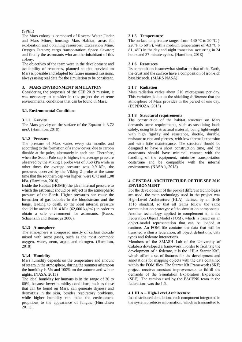
(SPEL)

The Mars colony is composed of Rovers: Water Finder

and Mars Miner; housing: Mars Habitat; areas for

exploration and obtaining resources: Excavation Mine,

Oxygen Factory; cargo transportation: Space elevator;

and finally the astronauts who are the inhabitant of this

colony.

The objectives of the team were in the development and

availability of resources, planned so that survival on

Mars is possible and adapted for future manned missions,

always using real data for the simulation to be consistent.

3. MARS ENVIRONMENT SIMULATION

Considering the proposals of the SEE 2019 mission, it

was necessary to consider in this project the extreme

environmental conditions that can be found in Mars.

3.1. Environmental Conditions

3.1.1 Gravity

The Mars gravity on the surface of the Equator is 3.72

m/s². (Hamilton, 2018)

3.1.2 Pressure

The pressure of Mars varies every six months and

according to the formation of a snow cover, due to carbon

dioxide at the poles, alternately in each one. Therefore,

when the South Pole cap is higher, the average pressure

observed by the Viking 1 probe was of 0,68 kPa while in

other times the average pressure was 0,9 kPa, the

pressures observed by the Viking 2 probe at the same

time that the southern cap was higher, were 0,73 and 1,08

kPa. (Hamilton, 2018)

Inside the Habitat (HOME) the ideal internal pressure to

which the astronaut should be subject is the atmospheric

pressure of the Earth. Higher pressures can cause the

formation of gas bubbles in the bloodstream and the

lungs, leading to death, so the ideal internal pressure

should be around 101.4 kPa (62,600 kg/m2) in order to

obtain a safe environment for astronauts. (Ruess,

Schaenzlin and Benaroya 2006).

3.1.3 Atmosphere

The atmosphere is composed mostly of carbon dioxide

mixed with some gases, such as the most common:

oxygen, water, neon, argon and nitrogen. (Hamilton,

2018)

3.1.4 Humidity

Mars humidity depends on the temperature and amount

of steam in the atmosphere, during the summer afternoon

the humidity is 5% and 100% on the autumn and winter

nights. (NASA, 2015)

The ideal humidity for humans is in the range of 30 to

60%, because lower humidity conditions, such as those

that can be found on Mars, can generate dryness and

dermatitis in the skin, besides respiratory problems,

while higher humidity can make the environment

propitious to the appearance of fungus. (Hinrichsen

2011).

3.1.5 Temperature

The surface temperature ranges from -140 °C to 20 °C (-

220°F to 68°F), with a medium temperature of -63 °C (-

81, 4°F) in the day and night transition, occurring in 24

hours and 37 minute cycles. (Hamilton, 2018)

3.1.6 Resources

Its composition is somewhat similar to that of the Earth,

the crust and the surface have a composition of iron-rich

basaltic rock. (MARS NASA)

3.1.7 Radiation

Mars radiation varies about 210 micrograms per day.

This variation is due to the shielding difference that the

atmosphere of Mars provides in the period of one day.

(ESPINOZA, 2013)

3.1.8 Structural requirements

The construction of the habitat structure on Mars

demands some requirements, such as sustaining loads

safely, using little structural material, being lightweight,

with high rigidity and resistance, ductile, durable,

resistant to rips and pierces, with low thermal expansion

and with little maintenance. The structure should be

designed to have a short construction time, and the

astronauts should have minimal contact with the

handling of the equipment, minimize transportation

costs/time and be compatible with the internal

environment. (NASA´s, 2018)

4. GENERAL ARCHITECTURE OF THE SEE 2019

ENVIRONMENT

For the development of the project different technologies

are used, the main technology used in the project was

High-Level Architecture (HLA), defined by an IEEE

1516 standard, so that all teams follow the same

communication prototype of the simulation components.

Another technology applied to complement it, is the

Federation Object Model (FOM), which is based on an

object-model representation that can be loaded at

runtime. An FOM file contains the data that will be

transited within a federation, all object definitions, data

types and federate interactions.

Members of the SMASH Lab of the University of

Calabria developed a framework in order to facilitate the

development of a federate, it is the “HLA Starter Kit”,

which offers a set of features for the development and

annotations for mapping objects with the data contained

within the FOM files. The Starter Kit Framework (SKF)

project receives constant improvements to fulfill the

demands of the Simulation Exploration Experience

(SEE). The version used by the FACENS team in the

federations was the 1.5.

4.1 HLA – High-Level Architecture

In a distributed simulation, each component integrated in

the system produces information, which is transmitted to

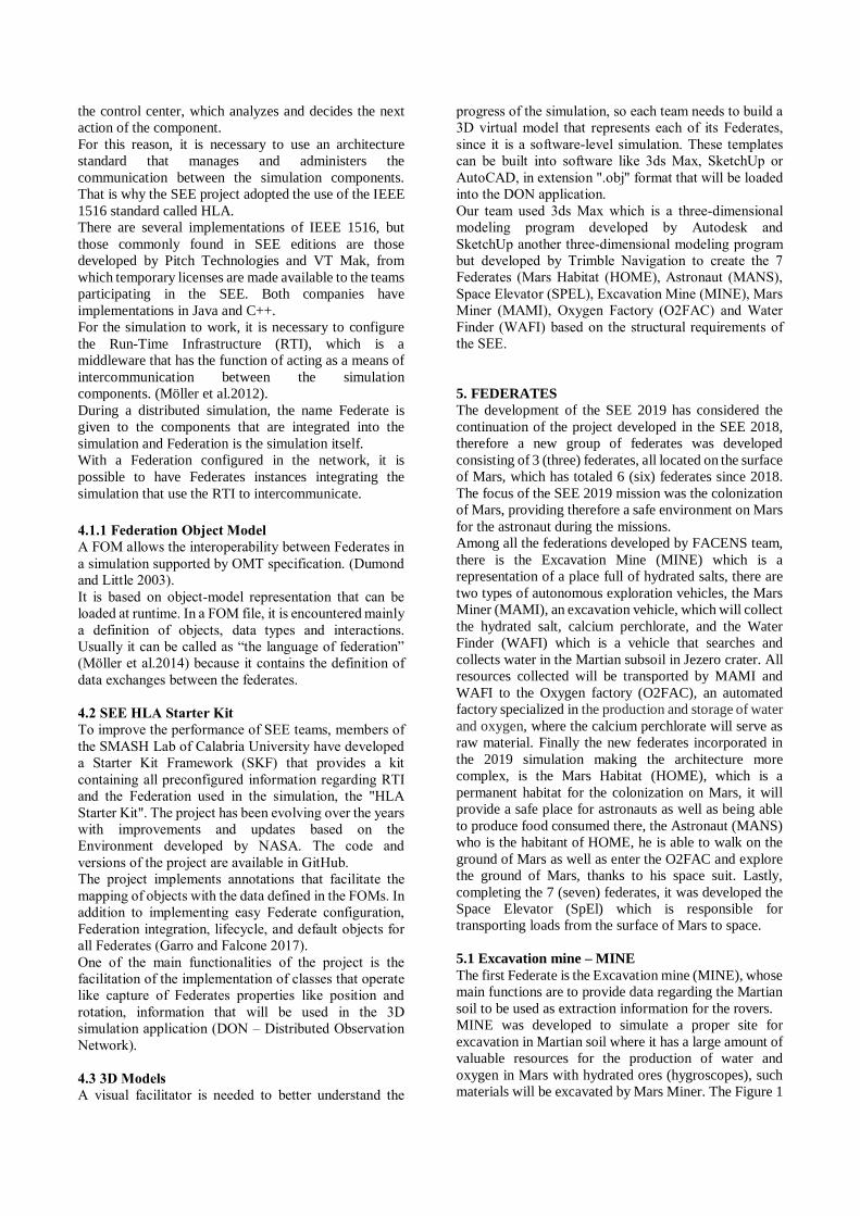
the control center, which analyzes and decides the next

action of the component.

For this reason, it is necessary to use an architecture

standard that manages and administers the

communication between the simulation components.

That is why the SEE project adopted the use of the IEEE

1516 standard called HLA.

There are several implementations of IEEE 1516, but

those commonly found in SEE editions are those

developed by Pitch Technologies and VT Mak, from

which temporary licenses are made available to the teams

participating in the SEE. Both companies have

implementations in Java and C++.

For the simulation to work, it is necessary to configure

the Run-Time Infrastructure (RTI), which is a

middleware that has the function of acting as a means of

intercommunication between the simulation

components. (Möller et al.2012).

During a distributed simulation, the name Federate is

given to the components that are integrated into the

simulation and Federation is the simulation itself.

With a Federation configured in the network, it is

possible to have Federates instances integrating the

simulation that use the RTI to intercommunicate.

4.1.1 Federation Object Model

A FOM allows the interoperability between Federates in

a simulation supported by OMT specification. (Dumond

and Little 2003).

It is based on object-model representation that can be

loaded at runtime. In a FOM file, it is encountered mainly

a definition of objects, data types and interactions.

Usually it can be called as “the language of federation”

(Möller et al.2014) because it contains the definition of

data exchanges between the federates.

4.2 SEE HLA Starter Kit

To improve the performance of SEE teams, members of

the SMASH Lab of Calabria University have developed

a Starter Kit Framework (SKF) that provides a kit

containing all preconfigured information regarding RTI

and the Federation used in the simulation, the "HLA

Starter Kit". The project has been evolving over the years

with improvements and updates based on the

Environment developed by NASA. The code and

versions of the project are available in GitHub.

The project implements annotations that facilitate the

mapping of objects with the data defined in the FOMs. In

addition to implementing easy Federate configuration,

Federation integration, lifecycle, and default objects for

all Federates (Garro and Falcone 2017).

One of the main functionalities of the project is the

facilitation of the implementation of classes that operate

like capture of Federates properties like position and

rotation, information that will be used in the 3D

simulation application (DON – Distributed Observation

Network).

4.3 3D Models

A visual facilitator is needed to better understand the

progress of the simulation, so each team needs to build a

3D virtual model that represents each of its Federates,

since it is a software-level simulation. These templates

can be built into software like 3ds Max, SketchUp or

AutoCAD, in extension ".obj" format that will be loaded

into the DON application.

Our team used 3ds Max which is a three-dimensional

modeling program developed by Autodesk and

SketchUp another three-dimensional modeling program

but developed by Trimble Navigation to create the 7

Federates (Mars Habitat (HOME), Astronaut (MANS),

Space Elevator (SPEL), Excavation Mine (MINE), Mars

Miner (MAMI), Oxygen Factory (O2FAC) and Water

Finder (WAFI) based on the structural requirements of

the SEE.

5. FEDERATES

The development of the SEE 2019 has considered the

continuation of the project developed in the SEE 2018,

therefore a new group of federates was developed

consisting of 3 (three) federates, all located on the surface

of Mars, which has totaled 6 (six) federates since 2018.

The focus of the SEE 2019 mission was the colonization

of Mars, providing therefore a safe environment on Mars

for the astronaut during the missions.

Among all the federations developed by FACENS team,

there is the Excavation Mine (MINE) which is a

representation of a place full of hydrated salts, there are

two types of autonomous exploration vehicles, the Mars

Miner (MAMI), an excavation vehicle, which will collect

the hydrated salt, calcium perchlorate, and the Water

Finder (WAFI) which is a vehicle that searches and

collects water in the Martian subsoil in Jezero crater. All

resources collected will be transported by MAMI and

WAFI to the Oxygen factory (O2FAC), an automated

factory specialized in the production and storage of water

and oxygen, where the calcium perchlorate will serve as

raw material. Finally the new federates incorporated in

the 2019 simulation making the architecture more

complex, is the Mars Habitat (HOME), which is a

permanent habitat for the colonization on Mars, it will

provide a safe place for astronauts as well as being able

to produce food consumed there, the Astronaut (MANS)

who is the habitant of HOME, he is able to walk on the

ground of Mars as well as enter the O2FAC and explore

the ground of Mars, thanks to his space suit. Lastly,

completing the 7 (seven) federates, it was developed the

Space Elevator (SpEl) which is responsible for

transporting loads from the surface of Mars to space.

5.1 Excavation mine – MINE

The first Federate is the Excavation mine (MINE), whose

main functions are to provide data regarding the Martian

soil to be used as extraction information for the rovers.

MINE was developed to simulate a proper site for

excavation in Martian soil where it has a large amount of

valuable resources for the production of water and

oxygen in Mars with hydrated ores (hygroscopes), such

materials will be excavated by Mars Miner. The Figure 1

shows the mine modeled for the simulation.

Figure 1. Excavation mine.

5.1.1 FOM of Excavation mine

The defined properties used by MINE in the simulation

and its FOM definition are listed below and in Figure 2:

● Depht: Represents the depth of the MINE;

● Diameter: Represents the excavated diameter of

the MINE;

● Number_of_mars_rover: Represents the

number of rovers inside the MINE;

● Maximun_capacity: Represents the maximum

capacity of rovers in the MINE;

● Temperature: Represents the soil temperature of

Mars;

● Pressure: Represents the pressure of Mars;

● Area: Represents the total area of MINE;

● Volume: Represents the volume of the MINE;

Figure 2. Representation of MINE to federation.

5.2 Mars Miner - MAMI

The Mars Miner (MAMI) is a medium-sized vehicle with

six wheels. It also has a drill, to excavate rocks in the

MINE, and a mechanical claw, with the objective of

collecting ores and placing them in a container, attached

to the back of the vehicle, has its function due to solar

energy associated to a battery attached in its interior.

Figure 3 shows the 3D model created from Mars Miner.

At the boundary of the mine, Mars Miner moves freely

exploring, digging with its drill, clawing with its

mechanical claw, and looking for hydrated ores, such as

calcium perchlorate for the use of water absorbed in ores

for the production of oxygen and the possible use of it in

the production of fuel.

Figure 3. Mars miner.

5.2.1 FOM of Mars Miner

The defined properties used by MAMI in the simulation

and its FOM definition are listed below and in Figure 4:

● Battery_level: Represents the battery level of

the rover;

● Mass: Represents the total weight of the rover

(loaded mass added to the weight of the rover

itself).

● Mars_miner_Status: Represents the spatial

position of the rover;

● Temperature: Represents the temperature of the

rover;

● Speed: Represents the speed of the rover;

● Maximum_capacity: Represents the maximum

capacity of the rover;

● Loaded_mass: Represents the amount of mass

loaded by the rover;

● Height: Represents the total height of the rover;

● Width: Represents the width of the rover;

● Lenght: Represents the length of the rover;

Figure 4. Representation of MAMI to federation.

5.3 Oxygen Factory – O2FAC

The Oxygen Factory (O2FAC) will be used for two

functions, the first as a rover’s control center in which it

is responsible for the decision of the actions taken by the

rovers, and the second being responsible for the

manufacture of oxygen and water in an automated way.

O2FAC is powered by solar energy and has all its

communication panels in a remote and automated way

controlled by HOME. O2FAC will use the water

extracted from the hygroscopic ore called calcium

perchlorate or the frozen water in the subsoil of Mars for

the production of oxygen. Figure 3 shows the outside

view of O2FAC and for better visibility Figure 4 shows

the O2FAC without the dome.

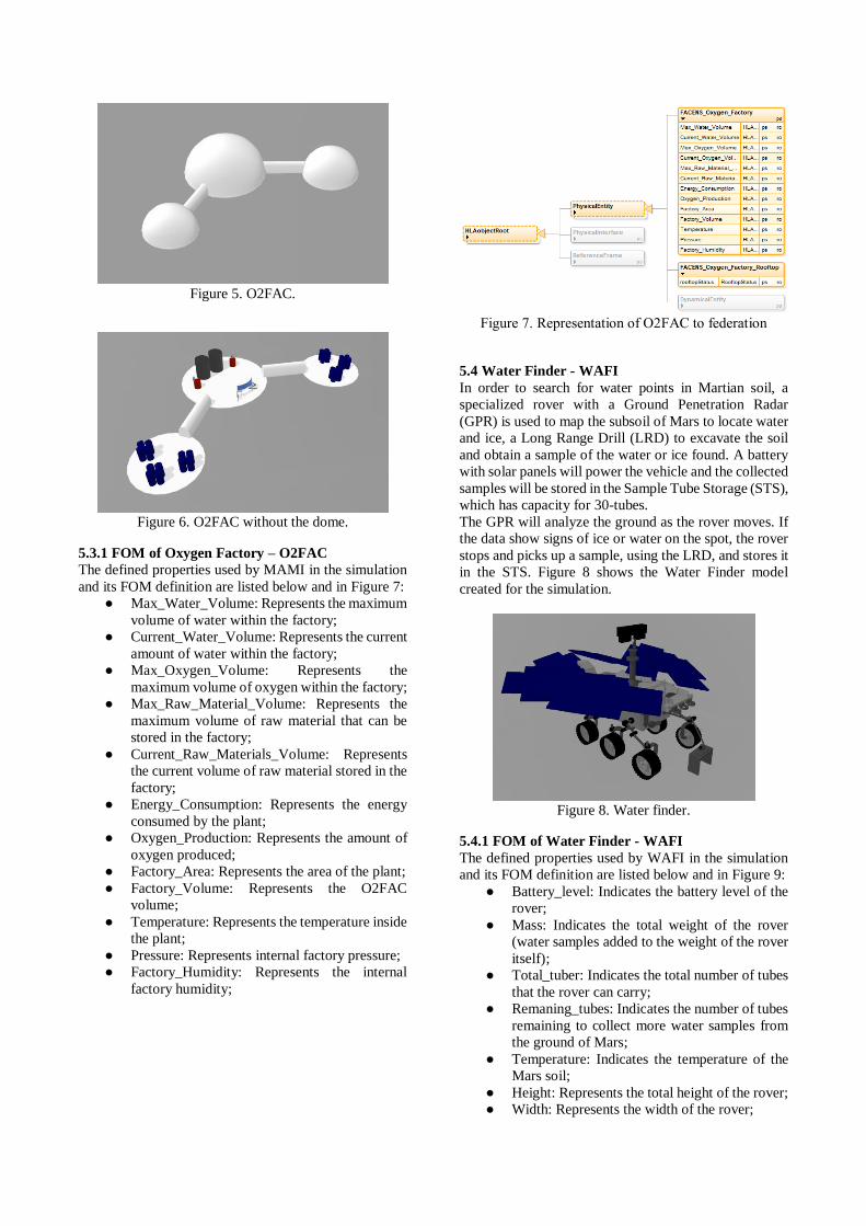
Figure 5. O2FAC.

Figure 6. O2FAC without the dome.

5.3.1 FOM of Oxygen Factory – O2FAC

The defined properties used by MAMI in the simulation

and its FOM definition are listed below and in Figure 7:

● Max_Water_Volume: Represents the maximum

volume of water within the factory;

● Current_Water_Volume: Represents the current

amount of water within the factory;

● Max_Oxygen_Volume: Represents the

maximum volume of oxygen within the factory;

● Max_Raw_Material_Volume: Represents the

maximum volume of raw material that can be

stored in the factory;

● Current_Raw_Materials_Volume: Represents

the current volume of raw material stored in the

factory;

● Energy_Consumption: Represents the energy

consumed by the plant;

● Oxygen_Production: Represents the amount of

oxygen produced;

● Factory_Area: Represents the area of the plant;

● Factory_Volume: Represents the O2FAC

volume;

● Temperature: Represents the temperature inside

the plant;

● Pressure: Represents internal factory pressure;

● Factory_Humidity: Represents the internal

factory humidity;

Figure 7. Representation of O2FAC to federation

5.4 Water Finder - WAFI

In order to search for water points in Martian soil, a

specialized rover with a Ground Penetration Radar

(GPR) is used to map the subsoil of Mars to locate water

and ice, a Long Range Drill (LRD) to excavate the soil

and obtain a sample of the water or ice found. A battery

with solar panels will power the vehicle and the collected

samples will be stored in the Sample Tube Storage (STS),

which has capacity for 30-tubes.

The GPR will analyze the ground as the rover moves. If

the data show signs of ice or water on the spot, the rover

stops and picks up a sample, using the LRD, and stores it

in the STS. Figure 8 shows the Water Finder model

created for the simulation.

Figure 8. Water finder.

5.4.1 FOM of Water Finder - WAFI

The defined properties used by WAFI in the simulation

and its FOM definition are listed below and in Figure 9:

● Battery_level: Indicates the battery level of the

rover;

● Mass: Indicates the total weight of the rover

(water samples added to the weight of the rover

itself);

● Total_tuber: Indicates the total number of tubes

that the rover can carry;

● Remaning_tubes: Indicates the number of tubes

remaining to collect more water samples from

the ground of Mars;

● Temperature: Indicates the temperature of the

Mars soil;

● Height: Represents the total height of the rover;

● Width: Represents the width of the rover;

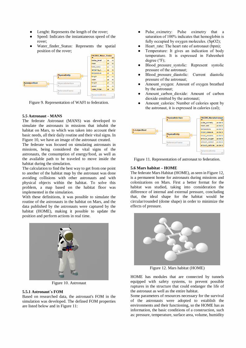
● Lenght: Represents the length of the rover;

● Speed: Indicates the instantaneous speed of the

rover;

● Water_finder_Status: Represents the spatial

position of the rover;

Figure 9. Representation of WAFI to federation.

5.5 Astronaut - MANS

The federate Astronaut (MANS) was developed to

simulate the astronauts in missions that inhabit the

habitat on Mars, to which was taken into account their

basic needs, all their daily routine and their vital signs. In

Figure 10, we have an image of the astronaut created.

The federate was focused on simulating astronauts in

missions, being considered the vital signs of the

astronauts, the consumption of energy/food, as well as

the available path to be traveled to move inside the

habitat during the simulation.

The calculation to find the best way to get from one point

to another of the habitat map by the astronaut was done

avoiding collisions with other astronauts and with

physical objects within the habitat. To solve this

problem, a map based on the habitat floor was

implemented in the simulation.

With these definitions, it was possible to simulate the

routine of the astronauts in the habitat on Mars, and the

data published by the astronauts were captured by the

habitat (HOME), making it possible to update the

position and perform actions in real time.

Figure 10. Astronaut

5.5.1 Astronaut´s FOM

Based on researched data, the astronaut's FOM in the

simulation was developed. The defined FOM properties

are listed below and in Figure 11:

● Pulse_oximetry: Pulse oximetry that a

saturation of 100% indicates that hemoglobin is

fully occupied by oxygen molecules. (SpO2);

● Heart_rate: The heart rate of astronaut (bpm);

● Temperature: It gives an indication of body

temperature. It is expressed in Fahrenheit

degree (°F);

● Blood_pressure_systolic: Represent systolic

pressure of the astronaut;

● Blood_pressure_diastolic: Current diastolic

pressure of the astronaut;

● Amount_oxygen: Amount of oxygen breathed

by the astronaut;

● Amount_carbon_dioxide: Amount of carbon

dioxide emitted by the astronaut;

● Amount_calories: Number of calories spent by

the astronaut, it is expressed in calories (cal);

Figure 11. Representation of astronaut to federation.

5.6 Mars habitat – HOME

The federate Mars Habitat (HOME), as seen in Figure 12,

is a permanent home for astronauts during missions and

colonizations on Mars. First a better format for the

habitat was studied, taking into consideration the

difference of internal and external pressure, concluding

that, the ideal shape for the habitat would be

circular/rounded (dome shape) in order to minimize the

effects of pressure.

Figure 12. Mars habitat (HOME)

HOME has modules that are connected by tunnels

equipped with safety systems, to prevent possible

ruptures in the structure that could endanger the life of

the astronaut as well as the entire habitat.

Some parameters of resources necessary for the survival

of the astronauts were adopted to establish the

environments and their functioning, so the HOME has as

information, the basic conditions of a construction, such

as: pressure, temperature, surface area, volume, humidity

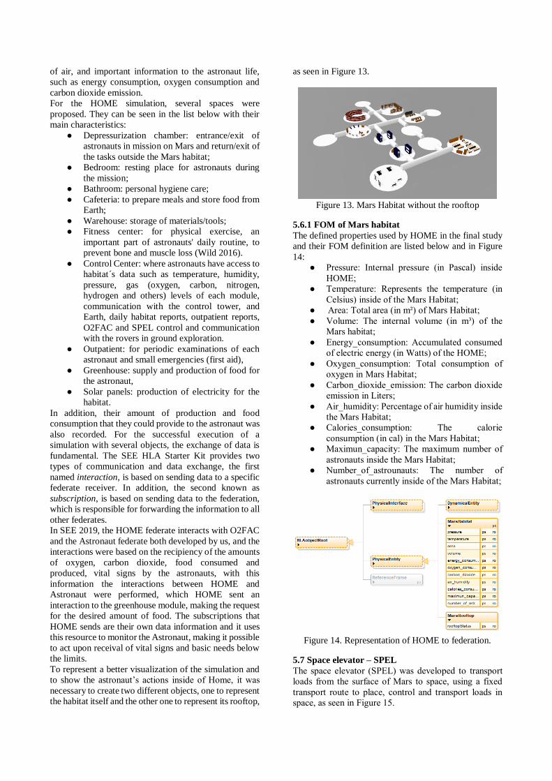
of air, and important information to the astronaut life,

such as energy consumption, oxygen consumption and

carbon dioxide emission.

For the HOME simulation, several spaces were

proposed. They can be seen in the list below with their

main characteristics:

● Depressurization chamber: entrance/exit of

astronauts in mission on Mars and return/exit of

the tasks outside the Mars habitat;

● Bedroom: resting place for astronauts during

the mission;

● Bathroom: personal hygiene care;

● Cafeteria: to prepare meals and store food from

Earth;

● Warehouse: storage of materials/tools;

● Fitness center: for physical exercise, an

important part of astronauts' daily routine, to

prevent bone and muscle loss (Wild 2016).

● Control Center: where astronauts have access to

habitat´s data such as temperature, humidity,

pressure, gas (oxygen, carbon, nitrogen,

hydrogen and others) levels of each module,

communication with the control tower, and

Earth, daily habitat reports, outpatient reports,

O2FAC and SPEL control and communication

with the rovers in ground exploration.

● Outpatient: for periodic examinations of each

astronaut and small emergencies (first aid),

● Greenhouse: supply and production of food for

the astronaut,

● Solar panels: production of electricity for the

habitat.

In addition, their amount of production and food

consumption that they could provide to the astronaut was

also recorded. For the successful execution of a

simulation with several objects, the exchange of data is

fundamental. The SEE HLA Starter Kit provides two

types of communication and data exchange, the first

named interaction, is based on sending data to a specific

federate receiver. In addition, the second known as

subscription, is based on sending data to the federation,

which is responsible for forwarding the information to all

other federates.

In SEE 2019, the HOME federate interacts with O2FAC

and the Astronaut federate both developed by us, and the

interactions were based on the recipiency of the amounts

of oxygen, carbon dioxide, food consumed and

produced, vital signs by the astronauts, with this

information the interactions between HOME and

Astronaut were performed, which HOME sent an

interaction to the greenhouse module, making the request

for the desired amount of food. The subscriptions that

HOME sends are their own data information and it uses

this resource to monitor the Astronaut, making it possible

to act upon receival of vital signs and basic needs below

the limits.

To represent a better visualization of the simulation and

to show the astronaut’s actions inside of Home, it was

necessary to create two different objects, one to represent

the habitat itself and the other one to represent its rooftop,

as seen in Figure 13.

Figure 13. Mars Habitat without the rooftop

5.6.1 FOM of Mars habitat

The defined properties used by HOME in the final study

and their FOM definition are listed below and in Figure

14: ● Pressure: Internal pressure (in Pascal) inside

HOME;

● Temperature: Represents the temperature (in

Celsius) inside of the Mars Habitat;

● Area: Total area (in m²) of Mars Habitat;

● Volume: The internal volume (in m³) of the

Mars habitat;

● Energy_consumption: Accumulated consumed

of electric energy (in Watts) of the HOME;

● Oxygen_consumption: Total consumption of

oxygen in Mars Habitat;

● Carbon_dioxide_emission: The carbon dioxide

emission in Liters;

● Air_humidity: Percentage of air humidity inside

the Mars Habitat;

● Calories_consumption: The calorie

consumption (in cal) in the Mars Habitat;

● Maximun_capacity: The maximum number of

astronauts inside the Mars Habitat;

● Number_of_astrounauts: The number of

astronauts currently inside of the Mars Habitat;

Figure 14. Representation of HOME to federation.

5.7 Space elevator – SPEL

The space elevator (SPEL) was developed to transport

loads from the surface of Mars to space, using a fixed

transport route to place, control and transport loads in

space, as seen in Figure 15.

Figure 15. Space elevator

It is composed of two main parts. One of them is

composed of a high base tower of approximately 17,000

km in height, to which it has a long cable tied at the top

that extends from the surface of Mars to space with its

center of mass in geostationary orbit. The other part that

composes the space elevator is the electromagnetic

vehicle, as shown in Figure 16, which travels a path along

the cable that has the function of a mass transport system

to move astronauts and payloads, between Mars and

space, without the need to use rocket propulsion.

However, for the base tower of the elevator to remain

stable on the planet is attached to it, a counterweight

mass attached to the geostationary orbit. (PRICE, 2000).

Figure 16. Electromagnetic vehicle

5.7.1 FOM of Space elevator – SPEL

The defined properties used by SPEL in the final study

and their FOM definition are listed below and in Figure

17: ● Power_supply: Indicates the energy available to

use SPEL;

● Power_Consumption: Indicates the energy

consumed for SPEL operation;

● Battery_Level: Indicates the battery level of the

SPEL;

● LauncherStatus: Indicates the position of the

electromagnetic vehicle in relation to the base

tower;

Figure 17. Representation of SPEL to federate.

6. RESULTS AND VALIDATIONS

After all the FACENS federates idealized and developed

in the modeling softwares and the definitions of the

boundaries in FOM, as seen previously in Figure 2,

Figure 4, Figure 7, Figure 9, Figure 11, Figure 14 and

Figure 17, it was possible to integrate the codes in the

DON and test the interactions between all the federates

based on the survival needs of astronauts and obtaining

resources developed by the FACENS team were running

simultaneously. They are Mars Habitat (HOME),

Astronaut (MANS), Space Elevator (SPEL), Water

Finder (WAFI), Mars Miner (MAMI), Excavation Mine

(MINE) and Oxygen Factory (O2FAC).

The interactions between the federates worked as

planned, the astronaut moved inside the habitat and it was

possible to see increase and decrease in his vital signs,

such as pulse oximetry, heart rate, body temperature,

blood pressure, amount of oxygen, carbon dioxide and

calories, the Mars Miner moved around the mine

collecting ores and the Water Finder moved around the

Mars soil collecting the subsoil water samples where and

the data from the astronaut and the two rovers were read

and managed by HOME as expected.

During the development of the project, the FACENS

team were divided between modeling and programming,

with weekly internal integrations, and worldwide once a

week with a specific schedule to check on the progress of

each one, and with these meetings, it was possible to

establish an exchange of knowledge.

The tests of the federates in the simulation software were

carried out several times, in order to correct errors related

to bugs, texture, position and interaction between the

federates.

This way the federates were ready to be presented at the

event that was held at Florida Institute of Technology

(FIT) in USA, on April 7, 2019, closing the SEE 2019

project.

7 CONCLUSIONS

With the developed project, it was possible to create a

simulation of a colonization on Mars, considering the

continuation of the project developed in the SEE 2018,

updating the past federations and presenting new

federates, simulating the production and consumption of

basic resources for the survival of the astronauts in an

inhospitable environment like Mars. Beholding a more

complex architecture, the team focused on Mars

colonization with the creation of HOME, which provides

a shelter during the manned mission on Mars, as well as

raising raw material (calcium perchlorate) and necessary

resources through the rovers, MAMI and WAFI, for the

production of oxygen and water in the O2FAC that

collaborates to maintain the astronaut's housing during

their mission on Mars, the MANS that is the astronaut

that inhabits HOME and transport cargo using SPEL.

However, this simulation did not consider parameters

such as meteor problems, to which they would be added

in future research and studies on these topics. NASA's

Modeling and Simulation project in partnership with

FACENS was a great opportunity for team members to

expand their horizons, interact with each other and with

other teams, exchange ideas, and develop skills and gain

experience.

REFERENCES

Dumond R., Little R.., 2003. A Federation Object Model

(FOM) Flexible Federate Framework, (no.

CMU/SEI-2003-tn-007). Carnegie-Mellon Univ

Pittsburgh PA Software Engineering Inst..

Espinoza L., 2013. Radiation measurements on Mars.

Available from:

https://www.nasa.gov/jpl/msl/mars-rover-

curiosity-pia17600.html#.WsosZi7wbIU

[Accessed 08 April 2019]

Garro A. and Falcone A., 2017. Simulation Exploration

Experience (SEE) The “SEE HLA Starter Kit”,

Università Della Calabria.

Greicius T., 2015. Nasa Mars rover´s weather data

bolsters case for brine. Available from:

https://www.nasa.gov/jpl/msl/nasa-mars-rovers-

weather-data-bolster-case-for-brine [Accessed 08

April 2019]

Hamilton C.J., 2018. Mars Introduction. Views of the

solar system. Available from:

http://solarviews.com/eng/mars.htm [Accessed 08

April 2019]

HLA tutorial. http://www.pitchtechnologies.com/wp-

content/uploads/2014/04/TheHLAtutorial.pdf.

Accessed 08 May 2019.

Hinrichsen E., 2011. Bright Hub Engineering. Available

from: http://www.brighthubengineering.com/hvac

/81719-best-indoor-humidity-range-for-people-

books-and-electronics/

[Accessed 08 April 2019]

Mars Nasa, 2018. Mars Facts. Composition. Available

from:

https://mars.nasa.gov/allaboutmars/facts/#?c=thepl

anet&s=composition [Accessed 08 April 2019]

Möller B., 2012. The HLA Tutorial - A Practical Guide

For Developing Distributed Simulations, Pitch

Technologies.

Möller, B., Dubois, A., Le Leydour, P., & Verhage, R.,

2014, RPR FOM 2.0: A federation object model for

defense simulations, In 2014 Fall Simulation

Interoperability Workshop, (paper 14F-SIW-039),

Orlando, FL.

NASA´s 3D-Printed Habitat Challenge – Phase 3, 2018.

Competition rules. from:

https://www.bradley.edu/sites/challenge/assets/doc

uments/3DPH_Phase_3_Rules-v3.pdf [Accessed

08 April 2019]

PRICE, Steve. Audacious & Outrageous: Space

Elevators. 2000. From:

https://science.nasa.gov/science-news/science-at-

nasa/2000/ast07sep_1 [Accessed 02 May 2019]

RAINEY, Larry B.; DAVIS, Paul K. (Ed.). Space

modeling and simulation: Roles and applications

throughout the system life cycle. El Segundo: The

Aerospace Press, 2004. 904 p.

SHAFTO, Mike et al. DRAFT Modeling, Simulation,

Information Technology & Processing

Roadmap. 2010. From:

<https://www.nasa.gov/pdf/501321main_TA11-

MSITP-DRAFT-Nov2010-A1.pdf>. [Accessed: 06

August 2019]

Wild F., 2016. Exercising in Space. NASA. Available

from:

https://www.nasa.gov/audience/foreducators/stem-

on-station/ditl_exercising. [Accessed 11 April

2019]

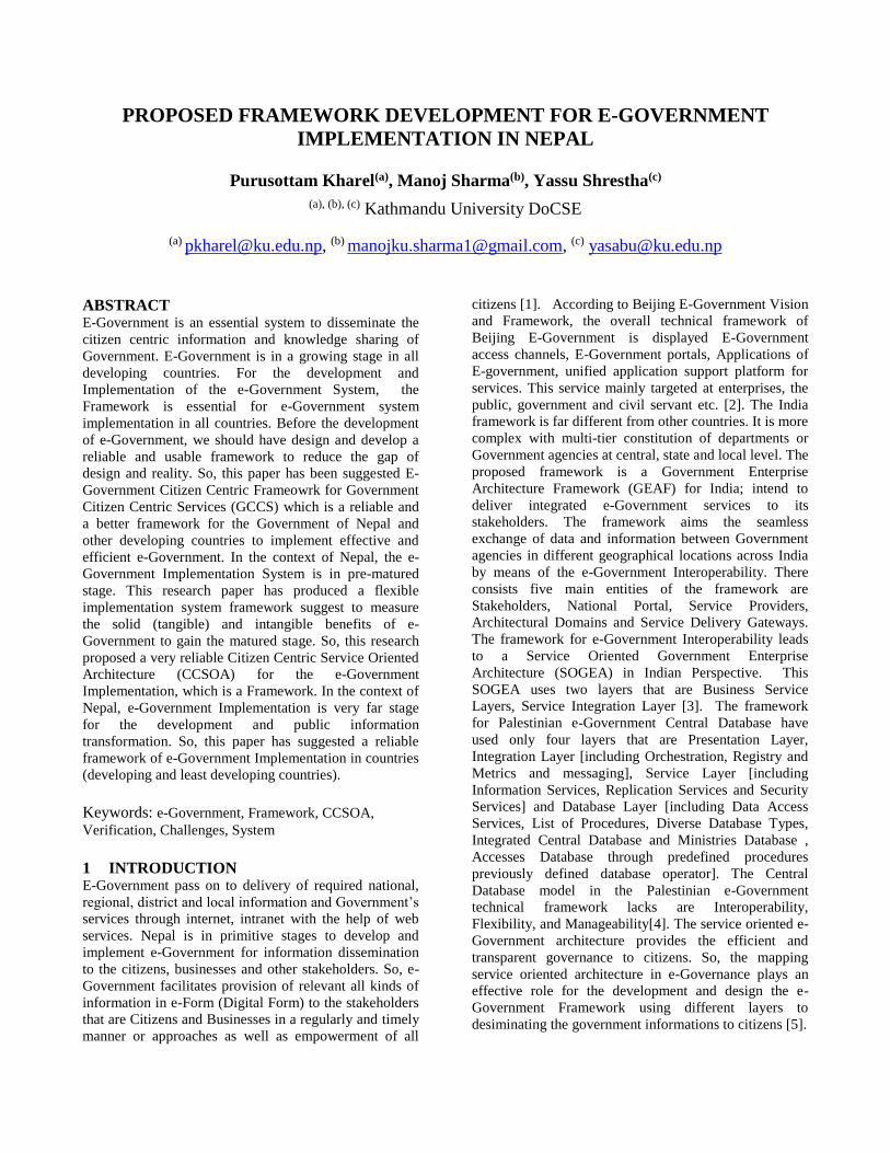
PROPOSED FRAMEWORK DEVELOPMENT FOR E-GOVERNMENT

IMPLEMENTATION IN NEPAL

Purusottam Kharel(a), Manoj Sharma(b), Yassu Shrestha(c)

(a), (b), (c) Kathmandu University DoCSE

(a) pkharel@ku.edu.np, (b) manojku.sharma1@gmail.com, (c) yasabu@ku.edu.np

ABSTRACT E-Government is an essential system to disseminate the

citizen centric information and knowledge sharing of

Government. E-Government is in a growing stage in all

developing countries. For the development and

Implementation of the e-Government System, the

Framework is essential for e-Government system

implementation in all countries. Before the development

of e-Government, we should have design and develop a

reliable and usable framework to reduce the gap of

design and reality. So, this paper has been suggested E-

Government Citizen Centric Frameowrk for Government

Citizen Centric Services (GCCS) which is a reliable and

a better framework for the Government of Nepal and

other developing countries to implement effective and

efficient e-Government. In the context of Nepal, the e-

Government Implementation System is in pre-matured

stage. This research paper has produced a flexible

implementation system framework suggest to measure

the solid (tangible) and intangible benefits of e-

Government to gain the matured stage. So, this research

proposed a very reliable Citizen Centric Service Oriented

Architecture (CCSOA) for the e-Government

Implementation, which is a Framework. In the context of

Nepal, e-Government Implementation is very far stage

for the development and public information

transformation. So, this paper has suggested a reliable

framework of e-Government Implementation in countries

(developing and least developing countries).

Keywords: e-Government, Framework, CCSOA,

Verification, Challenges, System

1 INTRODUCTION E-Government pass on to delivery of required national,

regional, district and local information and Government’s

services through internet, intranet with the help of web

services. Nepal is in primitive stages to develop and

implement e-Government for information dissemination

to the citizens, businesses and other stakeholders. So, e-

Government facilitates provision of relevant all kinds of

information in e-Form (Digital Form) to the stakeholders

that are Citizens and Businesses in a regularly and timely

manner or approaches as well as empowerment of all

citizens [1]. According to Beijing E-Government Vision

and Framework, the overall technical framework of

Beijing E-Government is displayed E-Government

access channels, E-Government portals, Applications of

E-government, unified application support platform for

services. This service mainly targeted at enterprises, the

public, government and civil servant etc. [2]. The India

framework is far different from other countries. It is more

complex with multi-tier constitution of departments or

Government agencies at central, state and local level. The

proposed framework is a Government Enterprise

Architecture Framework (GEAF) for India; intend to

deliver integrated e-Government services to its

stakeholders. The framework aims the seamless

exchange of data and information between Government

agencies in different geographical locations across India

by means of the e-Government Interoperability. There

consists five main entities of the framework are

Stakeholders, National Portal, Service Providers,

Architectural Domains and Service Delivery Gateways.

The framework for e-Government Interoperability leads

to a Service Oriented Government Enterprise

Architecture (SOGEA) in Indian Perspective. This

SOGEA uses two layers that are Business Service

Layers, Service Integration Layer [3]. The framework

for Palestinian e-Government Central Database have

used only four layers that are Presentation Layer,

Integration Layer [including Orchestration, Registry and

Metrics and messaging], Service Layer [including

Information Services, Replication Services and Security

Services] and Database Layer [including Data Access

Services, List of Procedures, Diverse Database Types,

Integrated Central Database and Ministries Database ,

Accesses Database through predefined procedures

previously defined database operator]. The Central

Database model in the Palestinian e-Government

technical framework lacks are Interoperability,

Flexibility, and Manageability[4]. The service oriented e-

Government architecture provides the efficient and

transparent governance to citizens. So, the mapping

service oriented architecture in e-Governance plays an

effective role for the development and design the e-

Government Framework using different layers to

desiminating the government informations to citizens [5].

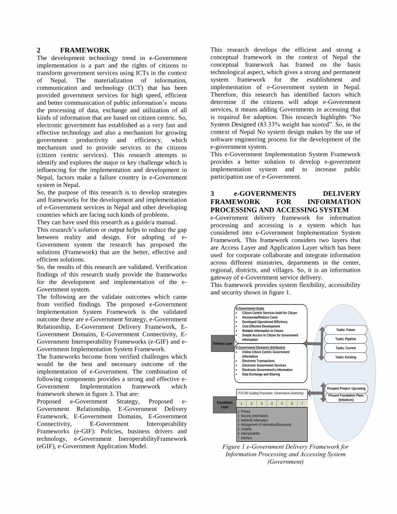
2 FRAMEWORK The development technology trend in e-Government

implementation is a part and the rights of citizens to

transform government services using ICTs in the context

of Nepal. The materialization of information,

communication and technology (ICT) that has been

provided government services for high speed, efficient

and better communication of public information’s means

the processing of data, exchange and utilization of all

kinds of information that are based on citizen centric. So,

electronic government has established as a very fast and

effective technology and also a mechanism for growing

government productivity and efficiency, which

mechanism used to provide services to the citizens

(citizen centric services). This research attempts to

identify and explores the major or key challenge which is

influencing for the implementation and development in

Nepal, factors make a failure country in e-Government

system in Nepal.

So, the purpose of this research is to develop strategies

and frameworks for the development and implementation

of e-Government services in Nepal and other developing

countries which are facing such kinds of problems.

They can have used this research as a guide/a manual.

This research’s solution or output helps to reduce the gap

between reality and design. For adopting of e-

Government system the research has proposed the

solutions (Framework) that are the better, effective and

efficient solutions.

So, the results of this research are validated. Verification

findings of this research study provide the frameworks

for the development and implementation of the e-

Government system.

The following are the validate outcomes which came

from verified findings. The proposed e-Government

Implementation System Framework is the validated

outcome these are e-Government Strategy, e-Government

Relationship, E-Government Delivery Framework, E-

Government Domains, E-Government Connectivity, E-

Government Interoperability Frameworks (e-GIF) and e-

Government Implementation System Framework.

The frameworks become from verified challenges which

would be the best and necessary outcome of the

implementation of e-Government. The combination of

following components provides a strong and effective e-

Government Implementation framework which

framework shown in figure 3. That are:

Proposed e-Government Strategy, Proposed e-

Government Relationship, E-Government Delivery

Framework, E-Government Domains, E-Government

Connectivity, E-Government Interoperability

Frameworks (e-GIF): Policies, business drivers and

technology, e-Government IneroperabilityFramework

(eGIF), e-Government Application Model.

This research develops the efficient and strong a

conceptual framework in the context of Nepal the

conceptual framework has framed on the basis

technological aspect, which gives a strong and permanent

system framework for the establishment and

implementation of e-Government system in Nepal.

Therefore, this research has identified factors which

determine if the citizens will adopt e-Government

services, it means adding Governments in accessing that

is required for adoption. This research highlights “No

System Designed (83.33% weight has scored”. So, in the

context of Nepal No system design makes by the use of

software engineering process for the development of the

e-government system.

This e-Government Implementation System Framework

provides a better solution to develop e-government

implementation system and to increase public

participation use of e-Government.

3 e-GOVERNMENTS DELIVERY

FRAMEWORK FOR INFORMATION

PROCESSING AND ACCESSING SYSTEM e-Government delivery framework for information

processing and accessing is a system which has

considered into e-Government Implementation System

Framework. This framework considers two layers that

are Access Layer and Application Layer which has been

used for corporate collaborate and integrate information

across different ministries, departments in the center,

regional, districts, and villages. So, it is an information

gateway of e-Government service delivery.

This framework provides system flexibility, accessibility

and security shown in figure 1.

Delivery Layer

E-Government Goals

· Citizen Centric Services build for Citizen

· Incorporate/Reduce Costs

· Developed Operational Efficiency

· Cost Effective Development

· Reliable Information to Citizen

· Simple Access to Citizen for Government

Information

E-Government Elements (Attributes)

· Online Citizen Centric Government

Information

· Electronic Transactions

· Electronic Government Services

· Electronic Government’s Information

· Data Exchange and Sharing

Foundation

Layer

IT/IC/IM Guiding Procedure: Governance (Authority)

1 2 3 4 5 6 7

1. Privacy

2. Security (Information)

3. Authentic Information

4. Management of Information/Documents

5. Usability

6. Interoperability

7. Interface

Tasks: Future

Tasks: Pipeline

Tasks: Current

Tasks: Existing

Prospect Project: Upcoming

Present Foundation Plans

(Initiatives)

Figure 1 e-Government Delivery Framework for

Information Processing and Accessing System

(Government)

In the context of Nepal, the Government can be

considered this framework for e-Government

Implementation System framework; e-Government

Master Plan (eGMP) has not considered this framework

component to deliver services to citizens. This

framework has two layers that are:

1. Foundation Layer (denoted by a capital A) - Consists

two entities – e-Government Goal and e-Government

attributes associated with the Project (future, pipeline,

current and existing) – denoted by Capital P1.

2. Delivery Layer – (denoted by a capital B) - Contains

an entity that is e-Government attributes associated

with a prospect project and present foundation plans –

denoted by capital P2.

The mathematical relationship of two layers with their

sets:

[A ® P1] ∩ [B ® P2] € S

A BS

P1 &

P2

P1 is the specific set of A and P2 is another set of B, such

as P1 and P2 are then connected with S. So, it is called

multilevel framework. Both A and B are associated with

each other to process the information and accessing

system that is S. This relationship considered into e-

Government Implementation System framework of

Access Layer and Application Layer.

4 e-GOVERNMENT SYSTEM

ARCHITECTURAL STRUCTURE (eGSAS) This research paper provides or recommends the

following structure of the e-Government System.

R: Regional Government

D9: Districts

D16 :Districts

D15:

Dis tricts

D19 :

Districts

D16: Districts

N

R1

R2

R3

R4

R5

Level of Government

N: National Government

D: District Government

L: Local Government

LG

LG

LG

LG

LG

Figure 2 Proposed Architectural Structures of the

e-Government System

The eGSAS helps the Government to implement an e-

Government system that holds to e-Government rules

and strategy; ensured that e-Government environment

which can have good and effective e-Government

implementation framework design.

The implementation of the e-government system has

structures to transfer information and data which show

the different levels for the implementation of system for

government services. The following figure 2 depicts the

architectural structures which have used for the

implementation of this structure using e-Government

Implementation System Framework.

Nepal has 5 regions and 75 districts and many villages

and cities are situated in this country. By the statistical

non-parametric method the research proves the illustrated

architectural structure of the e-government system that is

the connectivity of five layers of contains elements which

is:

N, R, D, L => S (System)

Here, N = National Level Government;

R = Regional Level Government;

D = District Level Government;

L = Local Level Government

The structure of connectivity of the architectural

structures, layers elements or entities.

S

NRLD RDLN

DLNRNRLD

Table 1 National, Regional, Districts and Local Government National

Government

Regional

Government

District

Government

Local

Government

N2N, R2R, D2D, L2L,

N2R, R2D, D2L, L2N,

N2D, R2L, D2N, L2R,

N2L R2N D2R L2D

The group elements of connectivity:

NNNN NRDL RRRR RDLN DDDD DLNR LLLL

LNRD

The sequence of connecting elements is:

N, N, N, N, N, R, D, L, R, R, R, R, R, D, L, N, D, D, D,

D, D, L, N, R, L, L, L, L, L, N, R, D

The connectivity of elements would use the following

symbols, they're contained four occurrence elements

layers.

µ1=N, µ2=R, µ3=D, µ4=L

Therefore, µ1=8, µ2=8, µ3=8, µ4=8

In this case the values of µ1, µ2, µ3, and µ4 must be

operates 8 times, accessibility for efficient and effective

e-Government implementation nationwide. The research

shows the five layers elements of the given architecture.

The architecture of an e-government system has equal

participation and the same range of connectivity and

accessibility. So,

System (S) = {µ1↔µ2↔µ3↔µ4}… (1)

This equation (1) allows to access and transformation of

information by citizens because all elements of layers are

connected to each other. It can prove that:

{N belongs to RDL}, {R belongs to NDL}, {D belongs

to NRL},{L belongs to NRD} U System

= N{R,D,L},R{N,D,L},D{N,R,L},L{N,R,D}

= {N} + {R} + {D} + {L}…………… (2)

Therefore, S= {NRDL} All layers of elements have the

same relationship which allows for transformed

information from N entity (element) to L entity (element)

which has existed in mentioned layers.

5 RECOMMENDATION OF E-

GOVERNMENT IMPLEMENTATION

SYSTEM FRAMEWORK For the development of e-Government System must have

a framework for implementation of e-Government

framework provides a uniform or homogeneous set of

software apparatus for the new development and running

e-Government applications. All the developed and some

developing countries are applying the e-Government

system framework for effective operations of application

for dissemination of government services and required

information to citizens using different framework layers.

This framework provides general elements and set of the

usual templates which are naturally required to

implement or developed a system, reduced replica

(duplicated) work. Basically, the system framework has

expected to help or support member areas or locations for

saving time and cost in developing the new e-

Government applications.

So, the e-Government development is frequently defined

in different context and from various perspectives. This

has been controlled processes which should have

implemented right-through the entire structure of public

administration. E-Government framework is a process

which builds or generate methodological, technological,

organizational and personnel conditions for the efficient

and effective application/purpose of ICTs in public and

government administration, and a controlled process of

ICT application. In the context of Nepal no have such

kind of e-Government framework build for the

development of the e-Government System. The e-

Government System Framework should have developed

or construct on the basis of country’s geographical

infrastructures. So, this research proposed the constructed

e-Government System in the context of Nepal.

So, based on the collected data analysis and verification

the research presents a modern citizen centric

information based e-Government framework for effective

and efficient implementation of government e-Services.

Therefore, this research suggests the following types of

e-Government System framework which has permeated

systematic approach in taking all plans, idea and scheme

in the modern cloud based e-Government

implementation. The e-Government framework consists

of five elements layers which has shown in the figure 3

below. In this figure 3 upper section layer which is

access layer consists of user of e-Government Services,

Receiving and Sending Channels that is data and

information communication devices. Second section of

layers which is e-Government Layer consists of Portal

for information that is Government Integrated sign on

portal. Third layer section is the application layer

consists of processing application with an interface. In

the fourth section of the layer is Information and Data

System layer consists of Government Data sources

through different organizations. Such as in fifth section

or lower layer which is Infrastructure layer consists of

information dissemination network infrastructure that is a

foundation which has used to process and transformation

of information in the access layer of user of e-

Government Services sending and receiving sections.

Figure 3 e-Governments Implementation System Framework

There consist of following five layers in e-Government

1. Framework Layer: Access Layer

Variable: Citizens, Businesses, Employee, Institution,

Government, Departments, Others Stakeholders

Medium: PCs, Mobile, Telecenter, Call Center, Digital

Television (DTV), Web

2. Framework Layer: e-Government Layer

Variable: Central e-Government Portal, Number of Websites

Medium: All Citizens and Stakeholders

Framework Layer: Application Layer

Variables: Information Document Management System

(IDMS), Customer Relationship Management (CRM),

Enterprise Resource Planning (ERP), Web Service

Application (WSA), Enterprise Application Integration

(EAI), Electronic Data Interchange (EDI), Firmware

(FW)

Medium: Data System – Database and Datawarehouse

3. Framework Layer: Information and Data System

Layer

Variables: Government Integrated Data Center (GIDC)

Medium: Government Data Sources through different

organizations

4. Framework Layer: Infrastructure Layer

Variables: Server, LANs, Intranet, Internet, Extranet and

MANs

Medium: Networks

On the basis of the e-Government System, IT is enabling

administrative process between Citizen and Government

(G2C), among Government Institutions (G2G),

Government and Business (G2B) which presenting the

given figure 4.

1. Access Layer: Includes two variables that are

Government Users (Recipient of Government

Services) and Data communication Devices (Channel/

Medium). Government users can access the various

types of services using data communication channel

or devices. Government service users are citizens,

businesses, employee, institutions, Government

Departments and other stakeholders. Service medium

or channel that has been using services access point

are PCs, Mobile, Tele-center, Call Center, DTV,

Web. Access Channels are critical components of e-

Government.

2. E-Government Layer: Portal for information

dissemination. Includes number of websites known as

a web portal. So, this layer uses for integrating digital

data of various organizations into a web portal. This

has been used to provide the highest quality of

services, better access to Government resources, So,

it enables to provide all kinds of better services to

users.

3. Application Layer: Processing Application with

Interface. Consist various Information Technology

and processing component applications which have

used data processing and data integration. The main

functions of being layer are knowledge sharing and

information processing using ICT applications and

tools. This layer makes a strong base to construct e-

Government Portal which is mentioned in e-

Government layers. It provides real time

communication between systems at both data and

process level. Information Document Management

System (IDMS), Customer Relationship Management

(CRM), Enterprise Resource Planning (ERP), Web

Service Application (WSA), Enterprise Application

Integration (EAI), Electronic Data Interchange (EDI),

Firmware (FW) is included.

4. Information and Data System Layer: It is a

Government Data Source has managed through

different organizations. The main variable is

Government Integrated Data Center (GIDC) which

should have established with different organization’s

data and information domain sources. All citizen

centric information stored into this integrated data

center. By the functions of this center users can

access the citizen centric government services

(information).

5. Infrastructure Layer: Information dissemination

network infrastructures that are foundation of e-

Government Implementation System, which have

shown in figure 3. Building an information of nation

requires information communication technology

infrastructure which can flow and communicate all

needed information to citizens and other stakeholders.

So, this layer mainly focuses on technologies that

should have to build before e-Government services

offered. Server, LANs, Intranet, Internet, Extranet

and WANs are the variables of this framework’s

Infrastructure (Foundation) layer. The information

dissemination medium is Network.

Figure 4 e-Government IT enables administrative process

This figure 4 shows the transactions between citizen,

government and business for communication of

information that are G2C , G2G and G2B. This system

framework covered the following types of government

services that are G2G, G2E, G2I, G2B, and G2C. The

use of figure 3 e-Government Implementation System

Framework provides the structure for the implementation

of citizen centric informatics e-Government shown in

figure 2.

6. CLOUD COMPUTING Cloud Computing has been developing today as a

commercial infrastructure that eliminates the need for

maintaining expensive computing hardware. Through the

use of virtualization, clouds promise to address with the

same shared set of physical resources a large user base

with different requirements. Thus, clouds promise to be

for scientists an alternative to clusters, grids, and

supercomputers (Simon et al., 2010).

Cloud Computing is emerging rapidly, with its data

centres growing at an unprecedented rate. However, this

has come with issues over privacy, efficiency at the

expense of resilience, and environmental sustainability,

because of the dependence on Cloud vendors such as

Google, Amazon and Microsoft. Community Cloud

Computing (C3) provides an alternative architecture,

created by combing the Cloud with paradigms from Grid

Computing, principles from Digital Ecosystems, and

sustainability from Green Computing, while remaining

true to the original vision of the Internet. It is more

challenging than Cloud Computing, having to deal with

distributed computing issues, including heterogeneous

nodes, varying quality of service, and further security

limitations. However, these are not undefeatable

challenges, and with the need to retain control over

digital lives and the potential environmental

consequences (Marinos and Briscoe, 2012).

Cloud Computing is the implication of Internet-based

technologies for the demand of services originating from

the cloud as a metaphor for the web, based on depictions

in computer network diagrams to abstract the complex

infrastructure (Haynie, 2009). It can also be observed as a

commercial evolution of the Grid Computing, succeeding

where Utility Computing struggled, while making greater

use of the self-management advances of Autonomic

Computing. It facilitates the illusion of infinite

computing resources available on demand, with the

elimination of upfront commitment from users, and

payment for the use of computing resources on a short

term basis as per the requirement (Armbrust et al., 2012).

Three categories of cloud computing services were

identified: Infrastructure-as-aService (IaaS), which is raw

infrastructure and associated middleware, Platformas-a-

Service (PaaS) , that is, APls for developing applications

on an abstract platform, and Software-as-a-Service

(SaaS), which is support for running software services

distantly. The scientific community has not yet started to

adopt PaaS or SaaS solutions, primarily to avoid porting

legacy applications and for lack of the needed scientific

computing services, respectively. Unlike traditional data

centers, which lease physical resources, most clouds

lease virtualized resources which are mapped and run

transparently to the user by the cloud's virtualization

middleware on the cloud's physical resources. For

example, Amazon EC2 runs instances on its physical

infrastructure using the open-source virtualization

middleware (Barham et al., 2003).

7 CONCLUSION In this research paper, propose an effective (successful)

e-Government Implementation System Framework. The

research paper provides detail layers which include in the

proposed framework. In the framework includes five

layers that are Access Layer, e-Government Layer,

Application Layer, Information and Data System Layer

and Infrastructure Layer and their functions. Nepal

Government can be used this framework to establish the

effective and efficient e-Government System to provide

the citizen centric services for the peoples and

businesses. Because, Nepal has very complex

administrative structure, consists four government

components that are National (Central), Regions,

Districts and Local Level Governments. Nepal

Government and other Developing countries can be

applied e-Government Implementation System

Framework for the implementation of e-Government for

the providing of Government services. So, the e-

Government System Framework is the most important

challenges for development and implementing the e-

Government to disseminate the citizen-centric services.

Without appropriate designed of e-Government System

Framework, it is not possible to implement the citizen

centric e-government system in Nepal and other

developing countries. At First it is necessary to have a

strong and appropriate designed e-Government System

Framework with efficient ICT infrastructure to

implement e-government. The research basically

recommended the model and framework which are the

validated outcome. According to model and supported

frameworks develop an e-Government Implementation

System framework. The proposed framework strongly

recommended Implementation system.The future work

will be the establishment of e-Government based on e-

Government Services incorporation in the e-Government

System.

8. REFERENCES [1] Zakaria I Saleh & Rand A. Obeidat,“A Framework

for an E-Government Based on Service Oriented

Architecture for Jordan”, Yarmouk University,

Department of Management Information System,

Jordan; Yaser Khamyseh, Jordan University of

Science and Technology, Department of Computer

Science, Jordan, I.J. Information Engineering and

Electronic Business, 2013, 3, 1-10, Published

Online September 2013 in MECS

(http://www.mecs-press.org/) DOI: 10.581/

ijieeb.2013.03.01.

[2] Beijing Municipal Office of Informatization,

“Beijing E-Government Vision and Framework”,

Sister City Program Technology Summit White

Papers, June 24-25, 2004 May.

[3] Anu Paul1, Varghese Paul2, “A Framework for e-

Government Interoperability in Indian Perspective”,

School of Computer Science, M G University,

Kottyam, India, School of Information Technology,

Cochin University, Kochi, India, International

Journal of Computer Information Systems and

Industrial Management Applications. ISSN 2150 –

7988 Volume 6(2014) pp. 582-591.

[4] Suhail Madoukh1 smadoukh@iugaza.edu.ps and

Rebhi Baraka2 rbaraka@iugaza.edu.ps, “ A SOA-

Based e-Government Data Integration”, 1Ministry

of Telecommunication and Information

Technology, Gaza, Palestine, 2Faculty of

Information Technology, Islamic University of

Gaza, Gaza, Palestine, International Arab Journal of

e-Technology, Vol. 3, No.3, January 2014.

[5] S. Nirmala Sugirtha Rajini1 Research Scholar and

T. Bhuvaneswari, PhD.2 Assistant

Professor,“Mapping Service Oriented Architecture

and E-Governance”, 1Dr. M.G.R. Educational and

Research Institute, Chennai and 2L. N Government

College, Ponneri; International Conference of

EGovernence & Cloud Computing Serv’12)

Proceedings Published by International Journal of

Computer Applications® (IJCA).

[6] California Information Technology Council

Enterprise Architecture and Standards Committee,

“California Enterprise Architecture Framework”,

July 15, 2005, Release 1.0 Final.

[7] National Computer Center, National IT Industry

Promotion Agency – NCC, NIPA, Master Plan,

“Electronic Government Development & Strategy –

Assessment, Research, Strategy, Implementation

Plan, Philippines, December 2012.

[8] Economic Commission for Africa, Partnership on

Measuring ICT for Development, “Framework for a

Set of e-Government Core Indicators”, March,

2012.

[9] Tamara Almarabeh1 and Amer AbuAli2, “A General

Framework for E-Government: Definition Maturity

Challenges, Opportunities, and Success”, 1Computer Information System Department,

University of Jorda Al-Jubeiha, 11942, Amman,

Jordan, E-mail: t.almaraabeh@ju.edu.jo, 2Philadelphia University, Jerash, Jordan, E-mail:

drabuali@yahoo.com , European Journal of

Scientific Research ISSN 1450-216X Vol.39 No.1

(2010), pp.29-42 © EuroJournals Publishing, Inc.

2010

[10] Göran Goldkuhl, {goran.goldkuhl@liu.se}, ”From

policy to design and effects:A framework for e-

government research”, Department of Management

and Engineering, Linköping University, Sweden &

Department of Computer & Systems Sciences,

Stockholm University, Sweden, 9th Scandinavian

Workshop on E-Government, February 9-10, 2012,

Copenhagen.

[11] Elsa Estevez and Tomasz Janowski,”Electronic

Governance for Sustainable Development-

Conceptual Framework and State of Research”,

Center for Electronic Governance, United Nations

University International Institute for Software

Technology; The final version is published as “E.

Estevez, T. Janowski, Electronic Governance for

Sustainable Development — Conceptual

Framework and State of Research, Government

Information Quarterly, vol. 30, supplement 1, pp.

S94-S109, Elsevier, 2013”.

[12] Armbrust, M., A. Fox, R. Griffith, A. Joseph, R.

Katz, A. Konwinski, G. Lee, D. Patterson, A.

Rabkin, I. Stoica, and M. Zaharia, “Above the

Clouds: A Berkeley view of Cloud Computing,”

University of California, Berkeley, 2012.

[Online].Available: http://d1smfj0g31qzek.

cloudfront.net/ abovetheclouds.pdf.

[13] Barham, P., Dragovic, B., Fraser, K ., Hand , S.,

Harris, T .L., Ho, A., Pratt, 1., Warfield, A.: Xen

and the art of virt ualization. In: SOSP. ACM, New

York (2003).

[14] Haynie, M. Enterprise cloud services: Deriving

business value from Cloud Computing. Micro

Focus, Tech. Rep., 2009.

[15] Marinos A. and Briscoe G., 2012. Community

Cloud Computing. Available online at:

http://arxiv.org/pdf/0907.2485.pdf (Accessed

2016.2.25)

[16] Simon O., Alexandru I., Nezih Y., Radu P., Thomas

F. an d Dick E., 2010. D.R. Avr esky et a l. (Eds.):

Cloud c omputing , LNICST 34 , pp. 115- 131.

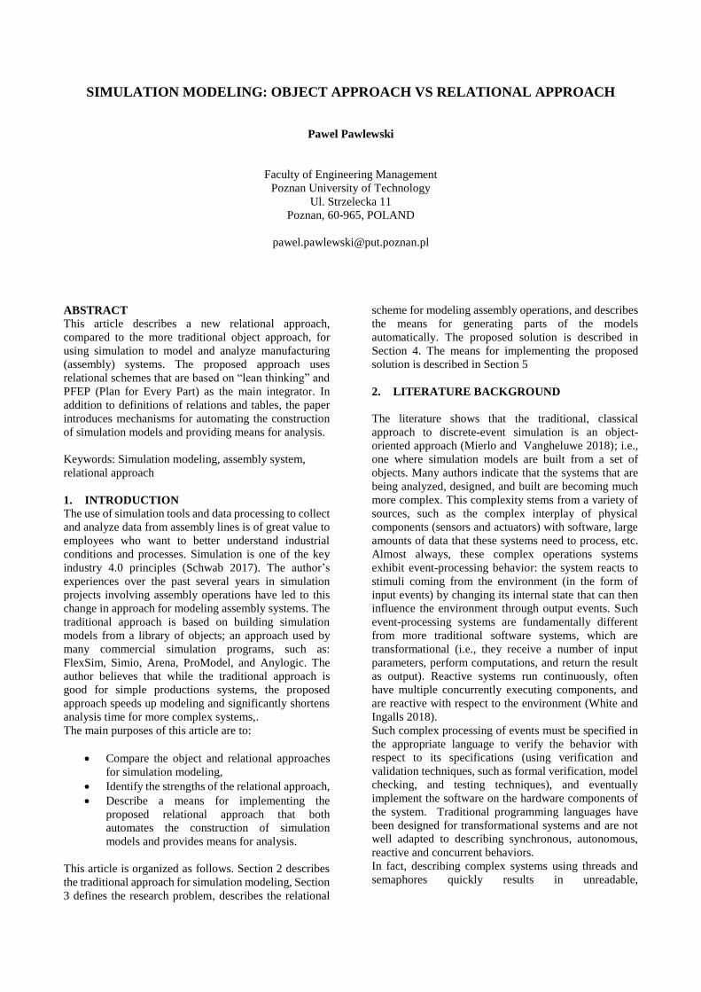
SIMULATION MODELING: OBJECT APPROACH VS RELATIONAL APPROACH

Pawel Pawlewski

Faculty of Engineering Management

Poznan University of Technology

Ul. Strzelecka 11

Poznan, 60-965, POLAND

pawel.pawlewski@put.poznan.pl

ABSTRACT

This article describes a new relational approach,

compared to the more traditional object approach, for

using simulation to model and analyze manufacturing

(assembly) systems. The proposed approach uses

relational schemes that are based on “lean thinking” and

PFEP (Plan for Every Part) as the main integrator. In

addition to definitions of relations and tables, the paper

introduces mechanisms for automating the construction

of simulation models and providing means for analysis.

Keywords: Simulation modeling, assembly system,

relational approach

1. INTRODUCTION

The use of simulation tools and data processing to collect

and analyze data from assembly lines is of great value to

employees who want to better understand industrial

conditions and processes. Simulation is one of the key

industry 4.0 principles (Schwab 2017). The author’s

experiences over the past several years in simulation

projects involving assembly operations have led to this

change in approach for modeling assembly systems. The

traditional approach is based on building simulation

models from a library of objects; an approach used by

many commercial simulation programs, such as:

FlexSim, Simio, Arena, ProModel, and Anylogic. The

author believes that while the traditional approach is

good for simple productions systems, the proposed

approach speeds up modeling and significantly shortens

analysis time for more complex systems,.

The main purposes of this article are to:

Compare the object and relational approaches

for simulation modeling,

Identify the strengths of the relational approach,

Describe a means for implementing the

proposed relational approach that both

automates the construction of simulation

models and provides means for analysis.

This article is organized as follows. Section 2 describes

the traditional approach for simulation modeling, Section

3 defines the research problem, describes the relational

scheme for modeling assembly operations, and describes

the means for generating parts of the models

automatically. The proposed solution is described in

Section 4. The means for implementing the proposed

solution is described in Section 5

2. LITERATURE BACKGROUND

The literature shows that the traditional, classical

approach to discrete-event simulation is an object-

oriented approach (Mierlo and Vangheluwe 2018); i.e.,

one where simulation models are built from a set of

objects. Many authors indicate that the systems that are

being analyzed, designed, and built are becoming much

more complex. This complexity stems from a variety of

sources, such as the complex interplay of physical

components (sensors and actuators) with software, large

amounts of data that these systems need to process, etc.

Almost always, these complex operations systems

exhibit event-processing behavior: the system reacts to

stimuli coming from the environment (in the form of

input events) by changing its internal state that can then

influence the environment through output events. Such

event-processing systems are fundamentally different

from more traditional software systems, which are

transformational (i.e., they receive a number of input

parameters, perform computations, and return the result

as output). Reactive systems run continuously, often

have multiple concurrently executing components, and

are reactive with respect to the environment (White and

Ingalls 2018).

Such complex processing of events must be specified in

the appropriate language to verify the behavior with

respect to its specifications (using verification and

validation techniques, such as formal verification, model

checking, and testing techniques), and eventually

implement the software on the hardware components of

the system. Traditional programming languages have

been designed for transformational systems and are not

well adapted to describing synchronous, autonomous,

reactive and concurrent behaviors.

In fact, describing complex systems using threads and

semaphores quickly results in unreadable,

incomprehensible, and unverifiable program code (Lee

2006).

This is partly due to the cognitive gap between the

abstractions offered by languages and the complexity of

the specifications, and sometimes badly defined

semantics of programming languages, which makes it

difficult to understand. As an alternative, the State-chart

formalism, was introduced by (Harel 1987). Many

simulation programs use state charts as a main tool for

simulation modeling (Anylogic, Simio). Another

modeling tool is Process Flow, offered by FlexSim

(FlexSim Software Products Inc.), which combines

programming language with graphics - it replaces nearly

all computer code with a flowchart. These tools focus on

the details of the modelled system and require the user

(production engineer, logistics) possess programming

skills and be familiar with a large number (hundreds) of

functions. Based on the author’s experiences, these users

do not want to deal with the details of the simulation

programs (primarily programing); they want to solve

problems in terms of their language and operational

concepts.

3. RESEARCH PROBLEM

Traditionally, a process perspective is used to model

production flows by creating models using a “top-down”

approach that drives model development from the

general to the specific. In this process-driven approach,

the flows of parts between processes create demands on

resources; i.e., a part moves to a workstation and

demands resources to complete an operation. While this

methodology is fine for many applications, it does not

allow resources to complete tasks that are not flow

related. For this, a task-driven approach is needed. For

example, an operator (mobile resource) performs a set of

inspections on idle equipment when not engaged in

process work. The task-based approach enables an

operator (task executor) to create tasks or activities that

are independent of the processing activities. Such tasks

may require travel and the acquisition of other tools or

resources. As such, the task-driven approach

incorporates “intelligence” into resources by enabling

them to decide what jobs to do and when.

In the literature it is often, recommended that simulation

projects start by building a map of the value stream

(Rother and Shook 2003). In such cases a process

approach is used to define part flows through a

production system. (Beaverstock, Greenwood and

Nordgren 2017). This approach is commonly described

in the simulation modeling literature and is used by

simulation software proudcts, such as: Simio, Anylogic,

Arena, ProModel, Tecnomatix, and FlexSim. This

approach works in a “top-down” manner; i.e., modeling

at a high level of abstraction and moving downward into

more detail as needed. This follows a classical approach.

(Hall 1962).

When building simulation models, we use elements,

often called objects, that reflect or approximate the

behavior of the real system. They are abstract objects

(e.g. graphic icons) or objects to which certain behaviors

are assigned. Graphic icons are elements of graphical

modeling languages, e.g. VSM (Value Stream Mapping)

(Rother and Shook 2003), IDEF0 (Santarek 1998) or

OFD (Object Flow Diagram) (Greenwood, Pawlewski

and Bocewicz 2013). Objects are assigned certain

behaviors, such as: source, buffer, processor ,and

operator. These objects can be used to model at different

levels of abstraction depending on the problem being

considered (Beaverstock, Greenwood and Nordgren

2017).

Generally, building models from objects involve placing

the objects selected from a library on to a work area and

defining the relations (connections) between these

objects based on item flow. Building a simulation model

of an entire factory in this manner is laborious and time

consuming.

Our goal is to change this situation by describing

assembling operations using relational schemes and

generating many parts of the model automatically.

4. SOLUTION OF PROBLEM

The proposed way of thinking about factory simulation

modeling is based on “lean thinking,” as described in

(Rother and Harris 2001), (Rother and Shook 2003),

(Harris, Harris and Wilson 2003), (Smalley 2003),

(Glenday 2005).

A main component of the approach is a database called

PFEP (Plan For Every Part). It is a part of a database that

contains information about all parts, components,

supplies, WIP (Work In Progress) inventories, raw

materials, finished goods, and any other material used in

manufacturing processes. The definitions and

requirements of a PFEP vary depending on specific needs

and the industry; but in general, PFEP fosters the

accurate and controlled management of commercial

information. PFEP is an essential lean tool and, when

combined with quality, delivery, true cost sourcing,

value stream mapping, and supplier development

initiatives, it can transform average supply chain

operations into world-class, just-in-time lean enterprises.

PFEP enables organizations to more effectively plan

completion dates, true costs of parts, and production

launch risks. Then, after a product is launched, PFEP is

used to proactively maintain high-functioning supply

chain operations by managing and optimizing inventory

costs, inbound logistics costs, and part supply change

costs. See Figure 1 for a simple example. Details for

using PFEP for simulation modeling of production

systems are explained by (Pawlewski 2018).

Figure 1: The view of PFEP.

PFEP is connected to two other databases: Locations and

Containers.

The Location database is a table that contains

information about all of the locations of containers in a

factory. A location is an area (a rectangle) with length

and width dimensions, angles of rotation relative to the

X, Y and Z axes, and is at a specified height. Locations

have no thickness. Parts and assemblies are delivered to

a station and are placed in a location. Products are

received from a station and are also collected in

containers. All resources that carry out transport

processes are treated as a "container". For example, a

transport trolley is a logical container for transporting a

finished product or a large-size part. An example of a

Location database is showed in Figure 2.

Figure 2: The view of Location database

This database contains parameters that define how to fill

locations and containers at the start of a simulation

Part – name of Part – indicates the row in PFEP.

Fill – number of filled containers.

Empty – number of empty containers.

Type of Cont. – indicator to fill the container

automatically when the last part is taken from container

Auto – indicator - how to fill in the location

0 No automatism related to filling the location

of containers Locations at the stand -

location replenishment is the result of

intralogistics activities - then the Fill and

Empty attributes have any values -Type of

container setting has

1 Automatic refilling of a container when a full

container is collected Locations in the

Supermarket then attributes Fill = 1, Empty = 0

2 Automatic removal of the container when the

container is located in the location. This means

locations in the finished goods warehouse - then

attributes Fill = 0, Empty = 0

3 Automatic filling of the empty container when

the container is picked up.

These parameters control the creation of containers with

parts at their specified location at the start of a simulation

experiment. This means that the user only needs to define

where, when, and how containers have to be generated.

The Containers database is a table where information

about the containers that are used in factory are stored,

including: ID, size, weight, shape (for 3D visualization),

etc.

All operations are performed by Operators. This is a class

that consists of the following types:

Humans,

Robots,

Forklifts

AGV’s

The parameters for these types are defined in separate

tables where rows describe subtypes..

Operators are objects that can perform operations. For

example, a forklift with a driver can be considered an

Operator, but without a driver it cannot. Operators

perform operations that are stored in tables assigned to

each Operator. A special language was developed to

describe the behaviors of Operators. This script language

consists of 64 operations that are grouped into the in

following categories: travel, loading/unloading,

operations, controlling. A full list of instructions can be

found in (Pawlewski 2018).

The structure of a factory is described in two tables:

- Groups that define production lines and/or cells and

are connected to the PFEP database

- Workstations that define elements of groups

(locations, Operators, Working tables, Assembly

stations, Disassembly stations)

The overall system of databases is presented in Figure 3

Figure 3: The view of Simulation Database System

5. IMPLEMENTATION

The database system shown in Figure 3 is implemented

within the LogABS simulation application that is

developed using the FlexSim simulation software

environment. (Pawlewski 2018b) FlexSim is treated as a

SOS (Simulation Operating System). The FlexSim

software was chosen because it is core 3D (working

directly in a 3D environment) and it is an open system,

i.e., system logic can easily be defined. (Beaverstock,

Greenwood and Nordgren 2017).

An example is provided for building a simulation model

of an assembly station in LogABS. The system is shown

in Figure 4, where the objects are: A - a rack with four

shelves for containers with parts, B – an Operator

(human), C – a work table, and D – a handcart for

transport. The operator assembles a finished product

from two parts, which are collected from containers in

the rack.

Figure 4: The view of assembly station

The assembly station simulation model is built by

completing the following steps:

Step 1: Define the set of containers via the Containers

database

Step 2: Define PFEP as a set of parts and finished goods

with connection to the Containers database

Step 3: Define a Group of workstations (production

line/cell) by defining the Line_ID, connecting to the

appropriate PFEP, and defining the number of

workstations in the Group. A workstation is created or

updated with empty records using the Update Control

Table button, as shown in Figure 5.

Figure 5: The view of Groups Database

Step 4: Define Workstations (every record or row in the

table), as shown in Figure 6 by providing the name of the

workstation, number of locations (for example from

figure 4, five locations), number of Operators (in this

case, 1), and number of Assembly Stations (in this case,

1).

Figure 6: The view of Workstation Database

The Update Workstations button in Figure 6 generates a

simulation model of the work area, with default

coordinates, as shown in Figure 7..The green rectangle is

the floor of the workstation; its size and color can be

modified.

Figure 7: The view of generated simulation model

Step 5. Pick by mouse location or sign the right cell in

Workstation Database to open window with Locations

Database connected to this workstation – figure 8

Figure 8: The view of Locations Database

This involves defining the proper coordinates of

locations, names of parts (connections to PFEP), method

for generating filled or empty containers, number of

containers.

Step 6. Pick by mouse Operator or sign the right cell on

Workstation Database to open window with set of tables

where the instructions for an operator can be defined. For

example, the set of instructions for an operator who

assembles a finished product from two parts, which are

collected from containers on a rack is shown in Figure 9.

Figure 9: The view of Operator’s Instruction Database

Step 7. Run Simulation experiment.

Step 8. Analyze results.

An Operator’s instructions are saved in a database that is

created at the beginning of the simulation experiments.

The database records save the names of the instructions,

start time of the instruction, its completion time, and the

value added attribute, as shown in Figure 10.

Figure 10: The scheme of mechanism to generate

results: time diagrams and value added analysis

6. CONCLUSIONS

The paper presents an approach for building simulation

models based on a relational database system The paper

defines and describes the relations and tables needed to

model assembly operations. The methodology for

building simulation models using a relational approach is

presented. A comparison of the traditional object

approach and the proposed relational approach is

provided in Table 1..

The proposed approach is implemented via the LogABS

simulation application that is developed in the FlexSim

simulation software environment. The approach and

LogABS application have been presented to engineers

and logisticians at assembly factories in a number of

industries (primarily bus and automotive) through

workshops. Based on the five workshops conducted so

far, the reactions of the participants has been very good;

therefore, commercialization activities for LogABS has

begun.

Table 1. Comparison of object and relational approach

for simulation modeling.

Criteria Object

Approach

Relational

Approach

Level of detail Low Medium/high

Number of

functions for

describing

behaviors

A large numer

of functions

(hundreds)

Small number of

functions

(several dozen)

User skills Programming

skills

Ability to set up

operator’s

itinerary

Ability to

automatically

generate

simulation

models

No Yes

Focus on: States of

objects

Operations

Compliance

with lean

manufacturing

Depends on

modeler

High

Built-in value-

added analysis

No Yes

ACKNOWLEDGMENTS

The work was carried out as part of the POIR.01.01.01-

00-0373/17 project, “Development of an automatic

drawer shelf using modified 90-degree reverse row

shelving systems dedicated to internal warehouse

logistics,” financed by NCBiR.

REFERENCES

Schwab K., 2017. The fourth industrial revolution.

Penguin UK

Van Mierlo S., Vangheluwe H., 2018. Introduction to

Statecharts Modeling, Simulation, Testing, and

Deployment. Proceedings of the 2018 Winter

Simulation Conference, pp 306-320.

White Jr. K.P., Ingalls R.G., 2018, The Basics of

Simulation, Proceedings of the 2018 Winter

Simulation Conference, pp 147-161.

Lee E. A., 2006. The Problem with Threads. Computer

39(5):33–42.

Harel D., 1987. Statecharts: A Visual Formalism for

Complex Systems. Science of Computer

Programming 8(3):231–274.

Rother M., Shook J., 2003. Learning to see. Value-

Stream Mapping to Create Value and Eliminate

Muda, The lean Enterprise Institute, Inc.

Beaverstock M., Greenwood A., Nordgren W., 2017.

Applied Simulation. Modeling and Analysis using

Flexsim, Flexsim Software Products, Inc., Canyon

Park Technology Center, Orem, USA.

Hall A. D., 1962. A Methodology for Systems

Engineering, Princeton N.J.

Santarek K., 1998. Organisational problems and issues of

CIM systems design. Journal of Materials

Processing Technology 76, 219-226

Greenwood A., Pawlewski P., Bocewicz G., 2013. A

Conceptual Design Tool to Facilitate Simulation

Model Development: Object Flow Diagram.

Proceedings of the 2013 Winter Simulation

Conference.

Rother M., Harris R., 2001. Creating Continous Flow,

The Lean Enterprise Institute, Inc.

Harris R., Harris Ch., Wilson E., 2003, Making Materials

Flow – A Lean Material-Handling Guide For

Operations, Production Control and Engineering

Professionals. The Lean Enterprise Institute, Inc.

Smalley A., 2003. Creating Level Pull, The Lean

Enterprise Institute, Inc.

Glenday I., 2005. Breaking Throught to Flow. The Lean

Enterprise Institute, Inc.

Pawlewski P., 2018. Using PFEP For Simulation

Modeling of Production Systems. Procedia

Manufacturing, Volume 17, Pages 811-818

Pawlewski P., 2018b. Methodology for layout and

intralogistics Redesign using Simulation.

Proceedings of the 2018 Winter Simulation

Conference.

AUTHOR BIOGRAPHY

Pawel Pawlewski is Professor of the Faculty of

Engineering Management at Poznan University of

Technology in Poland. His research interests include

discrete-event simulation, agent-based simulation, and

their applications: service systems, transportation

networks, and manufacturing. He has published over 130

papers. He is member of the board of Atres Intralogistics.

His e-mail address is pawel.pawlewski@put.poznan.pl.

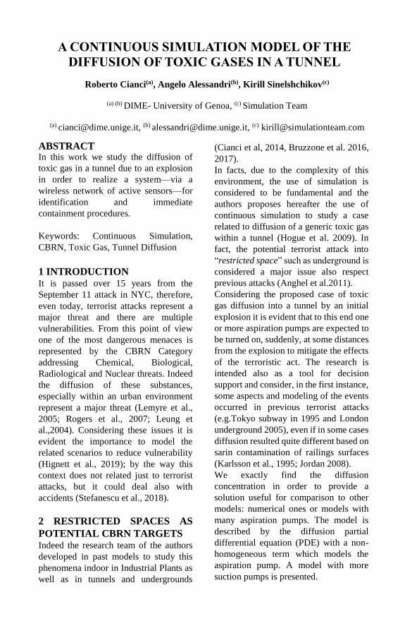
A CONTINUOUS SIMULATION MODEL OF THE

DIFFUSION OF TOXIC GASES IN A TUNNEL

Roberto Cianci(a), Angelo Alessandri(b), Kirill Sinelshchikov(c)

(a) (b) DIME- University of Genoa, (c) Simulation Team

(a) cianci@dime.unige.it, (b) alessandri@dime.unige.it, (c) kirill@simulationteam.com ABSTRACT In this work we study the diffusion of

toxic gas in a tunnel due to an explosion

in order to realize a system—via a

wireless network of active sensors—for

identification and immediate

containment procedures.

Keywords: Continuous Simulation,

CBRN, Toxic Gas, Tunnel Diffusion

1 INTRODUCTION It is passed over 15 years from the

September 11 attack in NYC, therefore,

even today, terrorist attacks represent a

major threat and there are multiple

vulnerabilities. From this point of view

one of the most dangerous menaces is

represented by the CBRN Category

addressing Chemical, Biological,

Radiological and Nuclear threats. Indeed

the diffusion of these substances,

especially within an urban environment

represent a major threat (Lemyre et al.,

2005; Rogers et al., 2007; Leung et

al.,2004). Considering these issues it is

evident the importance to model the

related scenarios to reduce vulnerability

(Hignett et al., 2019); by the way this

context does not related just to terrorist

attacks, but it could deal also with

accidents (Stefanescu et al., 2018).

2 RESTRICTED SPACES AS

POTENTIAL CBRN TARGETS Indeed the research team of the authors

developed in past models to study this

phenomena indoor in Industrial Plants as

well as in tunnels and undergrounds

(Cianci et al, 2014, Bruzzone et al. 2016,

2017).

In facts, due to the complexity of this

environment, the use of simulation is

considered to be fundamental and the

authors proposes hereafter the use of

continuous simulation to study a case

related to diffusion of a generic toxic gas

within a tunnel (Hogue et al. 2009). In

fact, the potential terrorist attack into

“restricted space” such as underground is

considered a major issue also respect

previous attacks (Anghel et al.2011).

Considering the proposed case of toxic

gas diffusion into a tunnel by an initial

explosion it is evident that to this end one

or more aspiration pumps are expected to

be turned on, suddenly, at some distances

from the explosion to mitigate the effects

of the terroristic act. The research is

intended also as a tool for decision

support and consider, in the first instance,

some aspects and modeling of the events

occurred in previous terrorist attacks

(e.g.Tokyo subway in 1995 and London

underground 2005), even if in some cases

diffusion resulted quite different based on

sarin contamination of railings surfaces

(Karlsson et al., 1995; Jordan 2008).

We exactly find the diffusion

concentration in order to provide a

solution useful for comparison to other

models: numerical ones or models with

many aspiration pumps. The model is

described by the diffusion partial

differential equation (PDE) with a non-

homogeneous term which models the

aspiration pump. A model with more

suction pumps is presented.

3 THE MODEL ONE-PUMP

The study of this section deals with a

single suction pump turned on

instantaneously at a distance of b meters

from the explosion and find exactly the

diffusion in order to provide an exact

solution for comparison to other models

with many pumps suction.

The model is described by diffusion PDE

with a non-homogeneous term which

models the suction pump. The Fourier

and Abel transforms are used by

calculating the effect of the pump and by

imposing the matching conditions. An

exact analytical solution is found and a

multi pumps model is outlined.

Consider firstly the 1-pump equation:

where C(z,t) is the concentration, D the

diffusion coefficient. Z is the spatial

coordinate and p a coefficient proportional

to the power of the pump which is

assumed present in z=b. Some further

remarks on the partial differential

equation. The term

simulate the aspiration pump by using the

generalized Dirac function. At the initial

time we simulate an explosion in z=0

. Compute now the

Fourier transform:

and get

This equation can be solved and the

solution is

Where N(q) is an arbitrarily function.

Now we return to the concentration

function and get:

We impose now initial condition

and obtain . In such a way we

get:

Now we compute the first integral and

obtain:

We remark that in this integral the value

of the concentration in z=b is required. We

put so z=b and get:

This integral equation is a second type

Abel integral equation. The solution is

We remark that the term

denoted the free evolution while the erfc

function is defined as:

In z=b, we have

Some plots are presented.

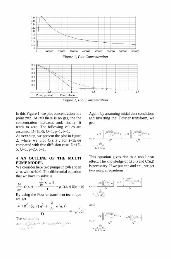
Figure 1, Plot Concentration

Figure 2, Plot Concentration

In this Figure 1, we plot concentration in a

point z=2. At t=0 there is no gas, the the

concentration increases and, finally, it

tends to zero. The following values are

assumed: D=1E-5, Q=1, p=1, b=1.

As next step, we present the plot in figure

2, where we plot C(z,t) , for t=1E-5s

compared with free diffusion case. D=1E-

5, Q=1, p=25, b=1.

4 AN OUTLINE OF THE MULTI

PUMP MODEL

We consider here two pumps in z=b and in

z=u, with u>b>0. The differential equation

that we have to solve is

By using the Fourier transform technique

we get

The solution is

Again, by assuming initial data conditions

and inverting the Fourier transform, we

get:

This equation gives rise to a non linear

effect. The knowledge of C(b,t) and C(u,t)

is necessary. If we put z=b and z=u, we get

two integral eqautions

and

5 CONCLUSIONS

This mathematical modeling approach is

interesting to create effective models

devoted to support design, engineering

and decision making respect threats in

underground transportations, however it is

evident that this approach should be

combined with effective modeling of the

boundary conditions including the

geometrical aspects and different

compressors and fans disposition within

the area as well as coupled with human

behavior modeling to estimate the impact

on people. In facts, we should also state

that the final system of integral equations

is very difficult to solve exactly, even by

using different techniques. Therefore this

additional development will be the focus

for future works of the authors and

different techniques of continuous

simulation numerical modeling will be

applied..

6 REFERENCES

[1] Abramowitz M, Stegun I. Handbook

of Mathematical Functions with

Formulas, Graphs, and Mathematical

Tables. NY,: Dover Publications,

1972

[2] Anghel, I., Zoicaş, C., Popa, C., &

Netcu, C. (2011). Using 3D dynamic

modeling for planning the response

to CBRN events in underground

public buildings. In SARTISS 2011

Conference, published in the Journal

of Emergency Medicine and

emergency situations, supplement

(No. 1, pp. 2066-0278).

[3] Batu V. A generalized two-

dimensional analytical solute

transport model in bounded media

for flux-type multiple sources. Water

Resour. Res, 1993, 29: pp. 2881-

2892

[4] Bear J. Dynamics of Fluids in Porous

Media. New York: Elsevier, 1972.

[5] Bruzzone, A. G., & Massei, M.

(2017). Simulation-based military

training. In Guide to Simulation-

Based Disciplines (pp. 315-361).

Springer, Cham.

[6] Bruzzone, A., Longo, F., Massei, M.,

Nicoletti, L., Agresta, M., Di Matteo,

R., Maglione G.L., M.G. &

Padovano, A. (2016, June). Disasters

and emergency management in

chemical and industrial plants:

drones simulation for education and

training. In International Workshop

on Modelling and Simulation for

Autonomous Systems (pp. 301-308).

Springer, Cham.

[7] Chen, J. ., C. F. Ni and C. P. Liang,

2008, Analytical power series

solutions to the two-dimensional

advection-dispersion equation with

distance-dependent dispersivities,

Hydrological Processes, 22: 4670-

4678.

[8] Cianci, R., Agostino, B., & Sburlati,

R. (2014). The Diffusion Problem of

Toxic Gases in a Tunnel. The Pump

Absorption Model. Acta applicandae

mathematicae, 132(1), 213-224.

[9] Healy, M. J. F., Weston, K., Romilly,

M., & Arbuthnot, K. (2009). A

model to support CBRN defence.

Defense & Security Analysis, 25(2),

119-135.

[10] Hignett, S., Hancox, G., & Edmunds

Otter, M. (2019). Chemical,

biological, radiological, nuclear and

explosive (CBRNe) events:

Systematic literature review of

evacuation, triage and

decontamination for vulnerable

people. International Journal of

Emergency Services.

[11] Hogue, R., Benbouta, N., Mailhot, J.,

Bélair, S., Lemonsu, A., Yee, E., ...

& Wilson, J. D. (2009, January). The

development of a prototype of a

Canadian urban flow and dispersion

modeling system. In Eighth

Symposium on the Urban

Environment.

[12] Jordan, F. (2008). Predicting target

selection by terrorists: A network

analysis of the 2005 London

underground attacks. International

journal of critical infrastructures,

4(1-2), 206-214.

[13] Karlsson, E., Berglund, T., Naslund,

E., Koch, B., & Runn, P. (1995).

Consequences of release of nerve

agent sarin in restricted spaces,

Some calculations in order to

illustrate the terrorist attack in the

Tokyo underground. In Proceedings

5th International Symposium on the

Protection Against Chemical and

Biological Warfare Agents.

[14] Lemyre, L., Clément, M., Corneil,

W., Craig, L., Boutette, P.,

Tyshenko, M., ... & Krewski, D.

(2005). A psychosocial risk

assessment and management

framework to enhance response to

CBRN terrorism threats and attacks.

Biosecurity and bioterrorism:

Biodefense strategy, practice, and

science, 3(4), 316-330.

[15] Leung, M., Lambert, J. H., &

Mosenthal, A. (2004). A risk‐based

approach to setting priorities in

protecting bridges against terrorist

attacks. Risk Analysis: An

International Journal, 24(4), 963-

984.

[16] Massabó M, Cianci R, Paladino O.

Some analytical solutions for two-

dimensional convection – dispersion

equation in cylindrical geometry.

Environmental Modelling &

Software, 2006; 21(5): 681-688.

[17] Parker J.C., Van Genuchten M.T.

Flux-averaged and volume-averaged

concentrations in continuum

approaches to solute transport.

(1984) Water Resources Research,

20 (7), pp. 866-872.

[18] Rogers, M. B., Amlôt, R., Rubin, G.

J., Wessely, S., & Krieger, K.

(2007). Mediating the social and

psychological impacts of terrorist

attacks: The role of risk perception

and risk communication.

International review of psychiatry,

19(3), 279-288.

[19] Stefanescu, L., Botezan, C., &

Craciun, I. (2018). Vulnerability

Analysis for two Accident Scenarios

at an Upper-Tier Seveso

Establishment in Romania.

Geographia Technica, 13(1).

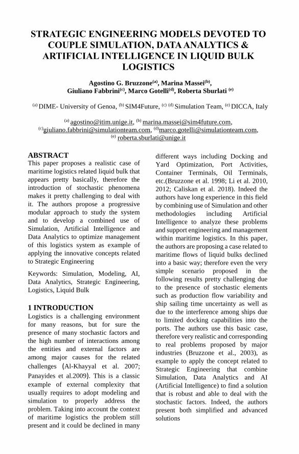
STRATEGIC ENGINEERING MODELS DEVOTED TO

COUPLE SIMULATION, DATA ANALYTICS &

ARTIFICIAL INTELLIGENCE IN LIQUID BULK

LOGISTICS

Agostino G. Bruzzone(a), Marina Massei(b),

Giuliano Fabbrini(c), Marco Gotelli(d), Roberta Sburlati (e)

(a) DIME- University of Genoa, (b) SIM4Future, (c) (d) Simulation Team, (e) DICCA, Italy

(a) agostino@itim.unige.it, (b) marina.massei@sim4future.com, (c)giuliano.fabbrini@simulationteam.com, (d)marco.gotelli@simulationteam.com,

(e) roberta.sburlati@unige.it

ABSTRACT This paper proposes a realistic case of

maritime logistics related liquid bulk that

appears pretty basically, therefore the

introduction of stochastic phenomena

makes it pretty challenging to deal with

it. The authors propose a progressive

modular approach to study the system

and to develop a combined use of

Simulation, Artificial Intelligence and

Data Analytics to optimize management

of this logistics system as example of

applying the innovative concepts related

to Strategic Engineering

Keywords: Simulation, Modeling, AI,

Data Analytics, Strategic Engineering,

Logistics, Liquid Bulk

1 INTRODUCTION Logistics is a challenging environment

for many reasons, but for sure the

presence of many stochastic factors and

the high number of interactions among

the entities and external factors are

among major causes for the related

challenges (Al-Khayyal et al. 2007;

Panayides et al.2009). This is a classic

example of external complexity that

usually requires to adopt modeling and

simulation to properly address the

problem. Taking into account the context

of maritime logistics the problem still

present and it could be declined in many

different ways including Docking and

Yard Optimization, Port Activities,

Container Terminals, Oil Terminals,

etc.(Bruzzone et al. 1998; Li et al. 2010,

2012; Caliskan et al. 2018). Indeed the

authors have long experience in this field

by combining use of Simulation and other

methodologies including Artificial

Intelligence to analyze these problems

and support engineering and management

within maritime logistics. In this paper,

the authors are proposing a case related to

maritime flows of liquid bulks declined

into a basic way; therefore even the very

simple scenario proposed in the

following results pretty challenging due

to the presence of stochastic elements

such as production flow variability and

ship sailing time uncertainty as well as

due to the interference among ships due

to limited docking capabilities into the

ports. The authors use this basic case,

therefore very realistic and corresponding

to real problems proposed by major

industries (Bruzzone et al., 2003), as

example to apply the concept related to

Strategic Engineering that combine

Simulation, Data Analytics and AI

(Artificial Intelligence) to find a solution

that is robust and able to deal with the

stochastic factors. Indeed, the authors

present both simplified and advanced

solutions

Figure 1: The Scenario to be optimized

2 LIQUID BULK SCENARIO The proposed case is corresponding to a

real problem extracted from a set of

scenarios that the authors addressed in the

past for maritime logistics of a major

Petrol Chemical Industry and could be

seen as one of the Simplest Problems in

Maritime Logistics (Bruzzone et al., 1998,

1999, 2002, 2011b, Massei et al., 2013);

however it should be pay attention to the

fact that solving the real problem, respect

simplified model based on deterministic

approach, is rather complex to be

managed and optimized; so immediately it

emerges the need to use extensively

Modeling and Simulation (M&S).

So the scenario is defined as following:

just 2 Ports, with 2 corresponding

Industrial Plants that need to be connected

by a Supply Chain for an Intermediate

Chemical Product. It is economically

inconvenient to use a pipeline due to

distances and flows. The Plants are

located in two sites separated by sea, so

the solution is to book a set of Ships

(Chemical Tankers) of proper capacity

and characteristics for a period (1 year

each year) and to use them to move the

product from A to B. Each ship sails to

Port A, loads the Product from the Tanks

of the Factory A, sails to B, unloads the

Product in the tanks of the Factory B and

sail back to A closing the cycle. The

Factory A fills up the Tanks in Port A.

Factory B fills up the Tanks in Port B;

until there is still product in B, the B

Factory is enabled to continue production

and until there is free space in Tanks of

Port A, Factory A can continue to go.

These Chemical Plants should not stop to

avoid very big extra costs. Each Port have

a single dock position. As simplified

hypothesis that corresponds mostly in the

real industrial problem we accept the idea

to use the same contract and type for all

the ships; indeed if we apply this approach

to the case of a maritime logistics flow this

is common in many case and even the

speed of the ship, within small range of

differences due to similarity of selected

ships, normally don’t affect the sailing

time among the two ports; so in facts it is

almost true that the ships are equivalent,

so it is possible to think in terms of time

distance between ports corresponding to

their average speed and to assume the

same contract for them; by the way these

assumptions in case of specific problems

could be easily overridden using M&S

(Bruzzone et al., 2011a). In addition

despite the importance to try to close the

return with some other compatible flows

and/or avoid empty return it is evident that

the regulations related to use of ship tanks

and incompatibilities among different

chemical products make this opportunity

pretty unfeasible in most of the cases, so

hereafter we don’t consider possibility to

use multiple product ships.

So, in this case, the basic data include:

Chemical Production Flows in Factories

Capacities of Tanks in the

Ports/Factories

Available Dock in Port Terminals

Loading/Unloading Capacities in Ports

Ship Contract Type

Tank Capacities of the Ships

Number of the Ships

Sailing Distance between Port A & B

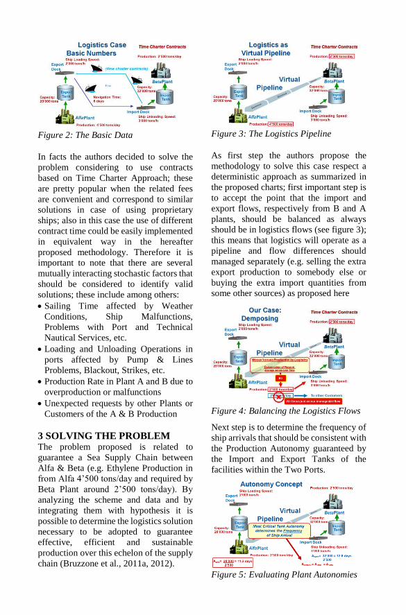
Figure 2: The Basic Data

In facts the authors decided to solve the

problem considering to use contracts

based on Time Charter Approach; these

are pretty popular when the related fees

are convenient and correspond to similar

solutions in case of using proprietary

ships; also in this case the use of different

contract time could be easily implemented

in equivalent way in the hereafter

proposed methodology. Therefore it is

important to note that there are several

mutually interacting stochastic factors that

should be considered to identify valid

solutions; these include among others:

Sailing Time affected by Weather

Conditions, Ship Malfunctions,

Problems with Port and Technical

Nautical Services, etc.

Loading and Unloading Operations in

ports affected by Pump & Lines

Problems, Blackout, Strikes, etc.

Production Rate in Plant A and B due to

overproduction or malfunctions

Unexpected requests by other Plants or

Customers of the A & B Production

3 SOLVING THE PROBLEM The problem proposed is related to

guarantee a Sea Supply Chain between

Alfa & Beta (e.g. Ethylene Production in

from Alfa 4’500 tons/day and required by

Beta Plant around 2’500 tons/day). By

analyzing the scheme and data and by

integrating them with hypothesis it is

possible to determine the logistics solution

necessary to be adopted to guarantee

effective, efficient and sustainable

production over this echelon of the supply

chain (Bruzzone et al., 2011a, 2012).

Figure 3: The Logistics Pipeline

As first step the authors propose the

methodology to solve this case respect a

deterministic approach as summarized in

the proposed charts; first important step is

to accept the point that the import and

export flows, respectively from B and A

plants, should be balanced as always

should be in logistics flows (see figure 3);

this means that logistics will operate as a

pipeline and flow differences should

managed separately (e.g. selling the extra

export production to somebody else or

buying the extra import quantities from

some other sources) as proposed here

Figure 4: Balancing the Logistics Flows

Next step is to determine the frequency of

ship arrivals that should be consistent with

the Production Autonomy guaranteed by

the Import and Export Tanks of the

facilities within the Two Ports.

Figure 5: Evaluating Plant Autonomies

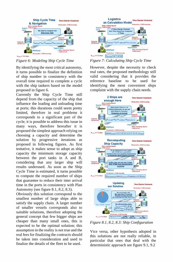
Figure 6: Modeling Ship Cycle Time

By identifying the most critical autonomy,

it turns possible to finalize the definition

of ship number in consistency with the

overall time required to complete a cycle

with the ship tankers based on the model

proposed in figure 6.

Currently the Ship Cycle Time still

depend from the capacity of the ship that

influence the loading and unloading time

at ports; this durations could seem pretty

limited, therefore in real problems it

corresponds to a significant part of the

cycle; it is possible to address this issue in

many ways, therefore hereafter it is

proposed the simplest approach relying on

choosing a capacity and determine the

solution by progressive iterations as

proposed in following figures. As first

tentative, it makes sense to adopt as ship

capacity the minimum storage capacity

between the port tanks in A and B,

considering that any larger ship will

results underused. As soon as the Ship

Cycle Time is estimated, it turns possible

to compute the required number of ships

that guarantee to reduce their inter arrival

time in the ports in consistency with Plan

Autonomy (see figure 8.1, 8.2, 8.3).

Obviously this solution correspond to the

smallest number of large ships able to

satisfy the supply chain. A larger number

of smaller vessels corresponds also to

suitable solutions, therefore adopting the

general concept that few bigger ships are

cheaper than many small ones, this is

expected to be the optimal solution; this

assumption in the reality is not true and the

real fees for finalizing the contracts should

be taken into consideration and used to

finalize the details of the fleet to be used.

Figure 7: Calculating Ship Cycle Time

However, despite the necessity to check

real rates, the proposed methodology still

valid considering that it provides the

reference baseline to be used for

identifying the most convenient ships

complaint with the supply chain needs.

Figure 8.1, 8.2, 8.3: Ship Configuration

Vice versa, other hypothesis adopted in

this solutions are not really reliable, in

particular that ones that deal with the

deterministic approach see figure 9.1, 9.2

Figure 9.1, 9.2: Deterministic and

Stochastic Levels into the tanks

3 SIMULATION TO FIND A

REAL SOLUTION The 9.1, 9.2 figures propose state space

representation respect the tank levels in

import and export facility and they make

it clear that in some moments the B tank

(import) turns to be empty, while A tank

(export) is time by time totally full.

So the solution identified by the basic

model is perfect, but just for Deterministic

cases and it results unable to avoid

Stockout in B Tank and Stockover in A

Tank corresponding to block of

production in related Plants and

unacceptable extra costs due to the

continuous nature of the industrial

process. So it is necessary to adopt a more

useful model and to avoid the limitations

of previous mentioned simplifications;

this results possible by creating a

simulation Model able to be used to

reproduce the system; in this case it is

adopted a discrete event stochastic model

that reproduce the scenario and allows to

estimate, by Monte Carlo techniques, the

effective costs, risks and times. In this

case the Simulator allows to identify the

performance of each ship solution in terms

of number and capacity (see figure 10).

Figure 10: Simulation Model

Therefore, it is evident that Simulation by

it self is able just to provide results to a

what if analysis, while we could be

interested to consider additional details

and investigate wide ranges to find

optimal solutions. Before to proceed we

state that the Optimum could be note

existing, or better undefined, considering

the stochastic nature of the real system; in

any case when we talk about finding

optimum, we look for a more reliable and

highly performing solutions in industrial

sense. To find this optimum it is very

interesting to use Artificial Neural

Networks (ANN) able to learn from a Data

Farming process generated by the

simulator, as well as from the real data

coming from operation activities of the

tanker fleet the correlations between ship

configurations and performances. These

ANNs allow to finalize a metamodel able

to support decisions in complex cases.

6 CONCLUSIONS

The proposed approach is a good example

of how Simulation, Data Analytics and AI

could be combined in order to support

decision by creating a dynamic closed

loop. The case looks simple, but by

considering its stochastic components it

results hard to be solved by traditional

approaches; therefore it is evident that

Simulation benefits from simplified

models results to be validated and

verified, while it uses enable generation of

large data set to better understand the

problem and to train AI solutions able to

learn correlations among fleet

configuration and logistics KPI (Key

Performance Indicators). Obviously, these

solutions are quite valuable considering

that are able to guarantee continuous

learning and to be kept up-to-date with

real operational data, providing valid

proposal to Decision makers. Therefore,

as above mentioned, the Decision Makers

could the loop being able to test their own

variations on the AI Proposal based on

personal choices that could consider

special elements and factors; indeed the

Simulator supports these check and allows

to close the loop and guarantee users on

properly finalizing their decisions respect

risks and boundary condition evolution.

6 REFERENCES

[1] Al-Khayyal, F., & Hwang, S. J.

(2007). Inventory constrained

maritime routing and scheduling for

multi-commodity liquid bulk, Part I:

Applications and model. European

Journal of Operational Research,

176(1), 106-130.

[2] Bruzzone, A.G., & Bocca, E. (2012).

Innovative solutions based on

modelling and simulation for

supporting decisions makers in

maritime logistics. Int. Journal of

Business Performance and Supply

Chain Modelling, 4(3-4), 333-358.

[3] Bruzzone, A., Longo, F., Massei, M.,

& Madeo, F. (2011a, June).

Modeling and simulation as support

for decisions makers in

petrochemical logistics. In

Proceedings of the Summer

Computer Simulation Conference

(pp. 130-137). Society for Modeling

& Simulation International.

[4] Bruzzone, A., Fadda, P., Fancello,

G., Massei, M., Bocca, E., Tremori,

A., et al. (2011b). Logistics node

simulator as an enabler for supply

chain development: innovative

portainer simulator as the assessment

tool for human factors in port cranes.

Simulation, 87(10), 857-874.

[5] Bruzzone, A., & Orsoni, A. (2003,

March). AI and simulation-based

techniques for the assessment of

supply chain logistic performance. In

Proceedings of the 36th IEEE

Annual Symposium on Simulation

[6] Bruzzone, A., Orsoni, A., Mosca, R.,

& Revetria, R. (2002, December).

AI-based optimization for fleet

management in maritime logistics. In

Proceedings of the Winter

Simulation Conference (Vol. 2, pp.

1174-1182). IEEE.

[7] Bruzzone, A. G., Merkuriev, Y. A.,

& Mosca, R. (Eds.). (1999).

Harbour, Maritime & Industrial

Logistics Modelling and Simulation:

HMS 1999, September 16-19, Hotel

Savoia Majestic, Genoa, Italy. SCS-

Europe BVBA.

[8] Bruzzone, A. G., Mosca, R., Esposti,

P. D., Vacante, S., & Carbone, A.

(1998). Distributed development of

simulation models for harbour

processes. WIT Transactions on The

Built Environment, 39.

[9] Caliskan, A., & Ozturkoglu, Y.

(2018). Maritime logistics. In

Intelligent Transportation and

Planning: Breakthroughs in

Research and Practice (pp. 822-845).

IGI Global

[10] Li, J., Karimi, I. A., & Srinivasan, R.

(2010). Efficient bulk maritime

logistics for the supply and delivery

of multiple chemicals. Computers &

Chemical Engineering, 34(12),

2118-2128.

[11] Massei, M., Tremori, A., Poggi, S.,

& Nicoletti, L. (2013). HLA-based

real time distributed simulation of a

marine port for training purposes.

International Journal of Simulation

and Process Modelling, 8(1), 42-51

[12] Panayides, P. M., & Song, D. W.

(2009). Port integration in global

supply chains: measures and

implications for maritime logistics.

International Journal of Logistics:

Research and Applications, 12(2),

133-145.

A REVIEW OF RECENT RESARCH INVOLVING MODELLING AND SIMULATION IN

DISASTER AND EMERGENCY MANAGEMENT

Adriano O. Solis(a)

(a)

School of Administrative Studies, York University, Toronto, Ontario, Canada

(a)

asolis@yorku.ca

ABSTRACT

The frequency, magnitudes, and consequences of

disasters and emergencies, both natural and man-made,

appear to have significantly increased in the past several

decades. We report on a still ongoing review of recent

research involving modeling and simulation (M&S) in

disaster and emergency management, as published in

various journals over the period 2011-2019. The

growing number of articles seems to indicate the keen

interest and engagement of scholars, scientists and

practitioners in this highly relevant and crucial area of

research.

Keywords: M&S, simulation, disaster and emergency

management, disaster operations management/disaster

management, management of emergency services,

emergency medical service, emergency department, fire

and rescue service

1. INTRODUCTION

Altay and Green (2006) noted that the operations

research/management science (OR/MS) community had

“yet to produce a critical mass” of research articles on

disaster operations management (DOM). They surveyed

109 articles on OR/MS research in DOM published in

various journals over the 25 years from 1980 to 2004,

both in mainstream OR/MS journals and in others. They

reported that five of the 42 papers (11.9%) appearing in

mainstream OR/MS journals involved simulation as

principal methodology, as did 13 of all 109 articles

(also 11.9%). They separately reported two papers

(1.8%) using system dynamics as methodology. This

implies a total of 15 (or 13.8%) of the 109 papers in

simulation, with system dynamics being generally

regarded to be a simulation method.

Subsequently, Galindo and Batta (2013) undertook a

survey covering the six-year period from 2005 to 2010,

reporting to have found a total of 155 articles on

OR/MS research in DOM. They stated that 14 of the

155 papers (or only 9%) used simulation as

methodology, while separately reporting two papers

(1.3%) under the system dynamics methodology.

Altogether, this leads to 16 (or 10.3%) of the 155

research articles being in simulation.

Mathematical programming was reported to be the most

used methodology (32.1% in the earlier survey and

23.1% in the latter survey). Simulation is noted by

Galindo and Batta (2013) to have maintained its status

as one of the “most widely used” methodologies next to

mathematical programming in OR/MS research in

DOM, and along with decision theory/multi-attribute

utility theory.

Table 1 provides a summary of these two previous

surveys. [We note that one figure appearing in Galindo

and Batta (2013) shows only a total of 30 papers

coming from mainstream OR/MS journals. The text,

however, mentions a different total of 37.]

Table 1: Previous Surveys of OR/MS Research in DOM

* In each survey, there are two papers reported separately by authors

to use system dynamics as methodology.

Gupta, Starr, Farahani, and Matinrad (2016) reviewed

papers on disaster management (DM) published from

1957 to 2014 in 25 “major journals” in operations

management (OM), MS, OR, supply chain management

(SCM), and transportation/logistics. They classified 146

papers according to ‘data analysis technique’,

identifying 15 papers (10.3%) as using simulation. In

comparison, 70 papers (47.9%) were classified as using

mathematical programming.

The term disaster management (DM) – as used by

Gupta et al. (2016) – is henceforth used in the current

report, in place of DOM.

With the Altay and Green (2006) and Galindo and Batta

(2013) surveys spanning the periods 1980-2004 (25

years) and 2005-2010 (six years), respectively, the

current survey covers the period 2011-2019 (nine

years). On the one hand, however, we focus on research

specifically involving M&S, instead of OR/MS in

general. On the other hand, we extend the field of

Altay &

Green (2006)

Galindo &

Batta (2013)

Time Period 1980-2004 2005-2010

Mainstream OR/MS journals 42 37

Other OR/MS related journals 35 14

Non-OR/MS journals 32 104

Total number of papers reviewed 109 155

Number of papers with simulation

(system dynamics* included) as

principal methodology 15 16

% of total 13.8% 10.3%

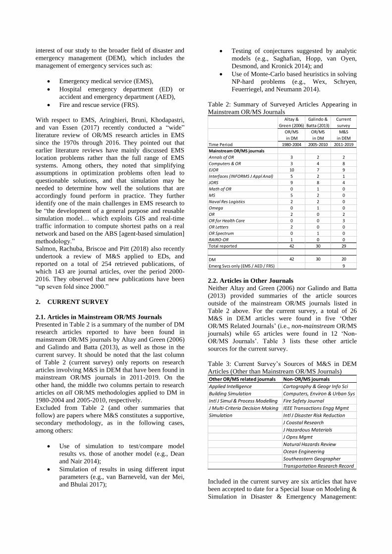
interest of our study to the broader field of disaster and

emergency management (DEM), which includes the

management of emergency services such as:

Emergency medical service (EMS),

Hospital emergency department (ED) or

accident and emergency department (AED),

Fire and rescue service (FRS).

With respect to EMS, Aringhieri, Bruni, Khodapastri,

and van Essen (2017) recently conducted a “wide”

literature review of OR/MS research articles in EMS

since the 1970s through 2016. They pointed out that

earlier literature reviews have mainly discussed EMS

location problems rather than the full range of EMS

systems. Among others, they noted that simplifying

assumptions in optimization problems often lead to

questionable solutions, and that simulation may be

needed to determine how well the solutions that are

accordingly found perform in practice. They further

identify one of the main challenges in EMS research to

be “the development of a general purpose and reusable

simulation model… which exploits GIS and real-time

traffic information to compute shortest paths on a real

network and based on the ABS [agent-based simulation]

methodology.”

Salmon, Rachuba, Briscoe and Pitt (2018) also recently

undertook a review of M&S applied to EDs, and

reported on a total of 254 retrieved publications, of

which 143 are journal articles, over the period 2000-

2016. They observed that new publications have been

“up seven fold since 2000.”

2. CURRENT SURVEY

2.1. Articles in Mainstream OR/MS Journals

Presented in Table 2 is a summary of the number of DM

research articles reported to have been found in

mainstream OR/MS journals by Altay and Green (2006)

and Galindo and Batta (2013), as well as those in the

current survey. It should be noted that the last column

of Table 2 (current survey) only reports on research

articles involving M&S in DEM that have been found in

mainstream OR/MS journals in 2011-2019. On the

other hand, the middle two columns pertain to research

articles on all OR/MS methodologies applied to DM in

1980-2004 and 2005-2010, respectively.

Excluded from Table 2 (and other summaries that

follow) are papers where M&S constitutes a supportive,

secondary methodology, as in the following cases,

among others:

Use of simulation to test/compare model

results vs. those of another model (e.g., Dean

and Nair 2014);

Simulation of results in using different input

parameters (e.g., van Barneveld, van der Mei,

and Bhulai 2017);

Testing of conjectures suggested by analytic

models (e.g., Saghafian, Hopp, van Oyen,

Desmond, and Kronick 2014); and

Use of Monte-Carlo based heuristics in solving

NP-hard problems (e.g., Wex, Schryen,

Feuerriegel, and Neumann 2014).

Table 2: Summary of Surveyed Articles Appearing in

Mainstream OR/MS Journals

2.2. Articles in Other Journals

Neither Altay and Green (2006) nor Galindo and Batta

(2013) provided summaries of the article sources

outside of the mainstream OR/MS journals listed in

Table 2 above. For the current survey, a total of 26

M&S in DEM articles were found in five ‘Other

OR/MS Related Journals’ (i.e., non-mainstream OR/MS

journals) while 65 articles were found in 12 ‘Non-

OR/MS Journals’. Table 3 lists these other article

sources for the current survey.

Table 3: Current Survey’s Sources of M&S in DEM

Articles (Other than Mainstream OR/MS Journals)

Included in the current survey are six articles that have

been accepted to date for a Special Issue on Modeling &

Simulation in Disaster & Emergency Management:

Altay &

Green (2006)

Galindo &

Batta (2013)

Current

survey

OR/MS

in DM

OR/MS

in DM

M&S

in DEM

Time Period 1980-2004 2005-2010 2011-2019

Mainstream OR/MS journals

Annals of OR 3 2 2

Computers & OR 3 4 8

EJOR 10 7 9

Interfaces (INFORMS J Appl Anal) 5 2 1

JORS 9 8 4

Math of OR 0 1 0

MS 5 2 0

Naval Res Logistics 2 2 0

Omega 0 1 0

OR 2 0 2

OR for Health Care 0 0 3

OR Letters 2 0 0

OR Spectrum 0 1 0

RAIRO-OR 1 0 0

Total reported 42 30 29

DM 42 30 20

Emerg Svcs only (EMS / AED / FRS) 9

Other OR/MS related journals Non-OR/MS journals

Applied Intelligence Cartography & Geogr Info Sci

Building Simulation Computers, Environ & Urban Sys

Intl J Simul & Process Modelling Fire Safety Journal

J Multi-Criteria Decision Making IEEE Transactions Engg Mgmt

Simulation Intl J Disaster Risk Reduction

J Coastal Research

J Hazardous Materials

J Opns Mgmt

Natural Hazards Review

Ocean Engineering

Southeastern Geographer

Transportation Research Record

Planning, Strategy Formulation, Decision-Making, and

Training of the journal IEEE Transactions on

Engineering Management. The six forthcoming articles

are as follows:

Gosavi, Fraioli, Sneed, and Tasker (2019);

Asgary, Bonadonna, and Frischknecht (2019);

Lavalle, Patriarca, Daulne, Hautier, Tofani,

and Ciancamerla (2019);

Shavarani, Golabi, and Vizvari (2019);

Aiello, Santisi, Hopps, and Venticinque

(2019); and

Behr, Diaz, Longo, and Padovano (2019).

2.3. Summary of All Articles in Current Survey

A grand total of 120 journal articles published over the

period 2011-2019 have so far been reviewed, as

summarized in Table 4 (see last column).

Table 4: Summary of All Articles Reviewed in Earlier

and Current Surveys

Excluding from the last column of Table 4 the 17

articles that pertain only to emergency services M&S,

we would be left with 103 M&S in DM articles in the

nine years from 2011 to 2019. Those 103 articles do

convey a truly exponential growth in the M&S in DM

literature, when compared with the 15

simulation/system dynamics articles reported for the 25

years from 1980 to 2004 (Altay and Green 2006) and

the 16 articles for the succeeding six years from 2005 to

2010 (Galindo and Batta 2013).

2.4. Articles with Human Behavior Modeling

What may be of interest is that 37 (or slightly over

30%) of the 120 articles in the current survey explicitly

include elements of human behavior modeling. Table 5

summarizes these 37 articles according to the journals

in which they have been published.

More than half (20) of the 37 articles deal with various

forms of evacuation in terms of:

Human subjects (residents, visitors,

pedestrians, crowds);

Infrastructure (homes, parking structures, high-

rise buildings, tunnels); and

Disasters/emergencies (earthquakes, tsunamis,

wildfires, man-made).

Table 5: Surveyed Articles with Human Behavior

Modeling (2011-2019)

In at least 11 of these 37 papers, agent-based models

have been proposed.

3. FURTHER WORK

The 120 articles surveyed thus far, as summarized in the

last column of Table 4, are by no means an exhaustive

compilation of research involving M&S in DEM

published in journals in 2011-2019. While we believe

that they constitute a fairly significant proportion of

such work over that time period, we intend, for the time

being, to continue searching for other M&S in DEM

research articles.

At WAMS 2019, we will update, as appropriate, the

report of articles surveyed. As well, we will provide

further observations and summaries with respect to

simulation methods or approaches (discrete event

simulation, agent-based simulation, system dynamics,

hybrid simulation, simulation-optimization), application

areas (e.g., disaster risk mitigation, pedestrian/crowd

flow and control, etc.), and other relevant

aspects/considerations pertaining to M&S in DEM.

APPENDIX

Table A.1: 25 “Major Journals” (Gupta, Starr, Farahani,

and Matinrad 2016)

Altay &

Green (2006)

Galindo &

Batta (2013)

Current

survey

OR/MS in

DM

OR/MS in

DM

M&S in

DEM

Time Period 1980-2004 2005-2010 2011-2019

Mainstream OR/MS journals 42 37 29

Other OR/MS related journals 35 14 26

Non-OR/MS journals 32 104 65

Total reported 109 155 120

With simulation as methodology

DM 15 16 96

DM + Emerg Svcs 7

Emerg Svcs only (EMS/AED/FRS) 17

Total 15 16 120

Mainstream OR/MS journals

Computers & OR 1

EJOR 2

Interfaces (INFORMS J Appl Anal) 1

OR 1

Other OR/MS related journals

Building Simulation 1

Intl J Simulation & Process Modelling 1

Simulation 10

Non-OR/MS journals

Fire Safety Journal 5

Intl J Disaster Risk Reduction 4

J Hazardous Materials 1

Southeastern Geographer 1

Transportation Research Record 9

Total with Human Behavior Modeling 37

Annals of OR Computers & OR

Decision Sciences Decision Support Systems

EJOR IIE Transactions

Int J Opns & Prod Mgmt Int J Prod Economics

Int J Prod Research J Opns Mgmt

J SCM JORS

MS Mfg & Service Opns Mgmt

Math Programming Math of OR

Naval Research Logistics Omega

OR OR Spectrum

Prod and Opns Mgmt SCM: An Intl Journal

Transportation Research Part B Transportation Research Part E

Transportation Science

REFERENCES

Aiello, G., Santisi, D., Hopps, F., and Venticinque, M.,

2019. The employment of Unmanned Aerial

Vehicles for analyzing and mitigating disaster

risks in industrial sites. IEEE Transactions on

Engineering Management, forthcoming.

Altay, N., and Green, W.G., 2006. OR/MS research in

disaster operations management. European Journal

of Operational Research, 175 (1), 475-493.

Aringhieri, R., Bruni, M.E., Khodaparasti, S., and van

Essen, J.T., 2016. Emergency medical services and

beyond: Addressing new challenges through a

wide literature review. Computers & Operations

Research, 78 (Complete), 349-368.

Asgary, A., Bonadonna, C., and Frischknecht, C., 2019.

Simulation and visualization of volcanic

phenomena using Microsoft HoloLens: Case of

Vulcano Island (Italy). IEEE Transactions on

Engineering Management, forthcoming.

Behr, J., Diaz, R., Longo, F., and Padovano, A., 2019.

Supply chain modeling in the aftermath of a

disaster: A system dynamics approach in housing

recovery. IEEE Transactions on Engineering

Management, forthcoming.

Dean, M.D., and Nair, S.K. (2014). Mass-casualty

triage: Distribution of victims to multiple hospitals

using the SAVE model. European Journal of

Operational Research, 238 (8), 363-373.

Galindo, G., and Batta, R., 2013. Review of recent

developments in OR/MS research in disaster

operations management. European Journal of

Operational Research, 230 (2), 201-211.

Gosavi, A., Fraioli, G., Sneed, L.H., and Tasker, N.,

2019. Discrete-event-based simulation model for

performance evaluation of post-earthquake

restoration in a smart city. IEEE Transactions on

Engineering Management, forthcoming.

Gupta, S., Starr, M.K., Farahani, R.Z., and Matinrad,

N., 2016. Disaster management from a POM

perspective: Mapping a new domain. Production

and Operations Management, 25 (10), 1611-1637.

Lavalle, L., Patriarca, T., Daulne, B., Hautier, O.,

Tofani, A., and Ciancamerla, E., 2019. Simulation-

based analysis of a real water distribution network

to support emergency management. IEEE

Transactions on Engineering Management,

forthcoming.

Saghafian, S., Hopp, W.J., van Oyen, M.P., Desmond,

J.S., and Kronick, S.L., 2014. Complexity-

augmented triage: A tool for improving patient

safety and operational efficiency. Manufacturing

& Service Operations Management, 16 (3), 329–

345.

Salmon, A., Rachuba, S., Briscoe, S., and Pitt, M.,

2018. A structured literature review of simulation

modelling applied to Emergency Departments:

Current patterns and emerging trends. Operations

Research for Health Care, 19 (Complete), 1-13.

Shavarani, S.M., Golabi, M., and Vizvari, B., 2019.

Assignment of medical staff to operating rooms in

disaster preparedness: A novel stochastic

approach. IEEE Transactions on Engineering

Management, forthcoming.

van Barneveld, T.C., van der Mei, R.D., and Bhulai, S.,

2017. Compliance tables for an EMS system with

two types of medical response units. Computers &

Operations Research, 80 (Complete), 68-81.

Wex, F., Schryen, G., Feuerriegel, S., and Neumann,

D., 2014. Emergency response in natural disaster

management: Allocation and scheduling of rescue

units. European Journal of Operational Research,

235 (3), 697-708.

The International Workshop on Applied Modeling and Simulation, 2019 978-88-85741-44-7; Bruzzone, Longo, Solis Eds VIII

Analytical Index

Angelo Alessandri 67

Lazaros Aresti 30, 35

Ikuo Arizono 7, 14, 23

Vincent Balducci 39

M.J.D. Bonato 45

Agostino G. Bruzzone IX, 72

A.B. Carneiro 45

Paul Christodoulides 30, 35

Roberto Cianci 67

Giuliano Fabbrini 72

L.M.A. Fadel 45

Georgios A. Florides 30, 35

Johannes Fottner 39

Marco Gotelli 72

Andreas Habl 39

Purusottam Kharel 54

R.Y. Koga 45

Masato Kondo 23

Moshe Kress 1

Lazaros Lazari 30

Francesco Longo IX

Marina Massei IX, 72

Vassilios Messaritis 35

Takuya Okamoto 14

Pawel Pawlewski 61

A.L.B.V. Rodrigues 45

Tomoko Sakiyama 7, 23

Roberta Sburlati 72

Manoj Sharma 54

Yassu Shrestha 54

J.L.A. Silva 45

Kirill Sinelshchikov 67

Adriano Solis IX, 78

Roberto Szechtman 1

T.M. Teixeira 45

G. Todesco 45

Tatsuya Yamaguchi 7

Yoshinari Yanagawa 14

Enver Yücesan 1

Final Program of the 12th International

Workshop on Applied Modelling & Simulation

October 30-31, 2019, www.liophant.org/wams

NUSS Kent Ridge Guild House, 9 Kent Ridge Drive, Singapore

WAMS2019 is organized in synergy with AsiaSim & STRATEGOS

Wednesday, October 30TH

845-0900 AsiaSim & WAMS OPENING, Dalvey & Evans Rooms

0900-1000 1st Day Keynote Speeches

1000-1030 Tea/Coffee Break (WAMS included)

1030-1200 AsiaSim Best Paper Session

1200-1330 AsiaSim & WAMS Lunch (WAMS included)

1400-1730 STRATEGOS Workshop: a New Way to Succeed (Evans)

1800-1930 AsiaSim & WAMS Welcome Cocktail (WAMS included)

2100-2230 Night Drink at Long Bar, Raffles Hotel (no host)

Thursday, October 31ST

0910-1000 2nd Day Keynote Speeches

100-1030 Tea/Coffee Break (WAMS included)

1030-1200 WAMS Evans Room, Session I Chairs: R.Sburlati, DICCA & I.Arizono, Okayama University

Job Shop Rescheduling with Lot Splitting under Multiple Interruptions

T.Okamoto, Y.Yanagawa, I.Arizono, Graduate School of Natural Scienze & Technology,

Okayama Univ., Japan (pg.14)

Scheduling Multiple Lift Vehicles in a Common Shaft in Automated Vehicle Storage

and Retrieval Systems

A.Habl, V.Balducci, J.Fottner, Technical University of Munich, Germany (pg.39)

Simulation Modeling: Object Approach vs. Relational Approach

P.Pawlewski, Faculty of Eng.Management, Poznan Univ.of Technology, Poland (pg.61)

Ground Source Heat Pumps Cost Analysis in Moderate Climate

L.Aresti, P.Christodoulides, V.Messaritis, G.A.Florides, Cyprus Univ. of Tech. (pg.35)

Computational Investigation on Effect of Various Parameters of a Spiral Ground

Heat Exchanger

L.Aresti, P.Christodoulides, L.Lazari, G.A.Florides, Cyprus Univ.of Tech.(pg.30)

1200-1330 AsiaSim & WAMS Lunch (WAMS included)

Thursday, October 31ST

1330-1530 WAMS Evans Room, Session II Chairman: A.G.Bruzzone, Simulation Team & L.Aresti, Cyprus Univ.of Technology

Strategic Engineering Models devoted to couple Simulation, Data Analytics &

Artificial Intelligence in Liquid Bulk Logistics

A.G.Bruzzone, DIME, M.Massei, SIM4Future, G.Fabbrini, M.Gotelli, Simulation Team,

R.Sburlati, DICCA, Italy (pg.72)

Proposal on Network Exploration to avoid Closed Loops

T. Yamaguchi, Graduate School of Nat.Science & Technology Okayama Univ., T.Sakiyama, Science &

Engineering Fac., Soka Univ., I.Arizono, Okayama Univ. (pg.7)

Proposed Framework Development for E-Government mplementation in Nepal

P.Kharel, M.Sharma, Y.Shrestha, Kathmandu University DoCSE, Dhulikhel, Nepal (pg.54)

A Novel Firefly Algorithm for Multimodal Optimization

M.Kondo, Graduate School of Natural Science & Technology Okayama Univ., T.Sakiyama, Science &

Eng. Fac., Soka Univ., I.Arizono, Okayama Univ., Japan (pg.23)

1530-1600 Tea/Coffee Break (WAMS included)

1600-1730 WAMS Evans Room, Session III Chairman: A.Solis, York University, R.Cianci, DIME

Adaptive Algorithms for Optimal Budget Allocation with an Application to the Employment of

Imperfect Sensors

M.Kress & R.Szechtman, NPS, USA, E.Yücesan, INSEAD, France (pg.1)

A Review of Recent Research Involving Modeling and Simulation

in Disaster and Emergency Management

Adriano Solis, York University, Canada (pg.78)

A Continuous Simulation Model of the Diffusion of Toxic Gases in a Tunnel

R.Cianci, A.Alessandri, Genoa Univ., Kirill Sinelshchikov, Simulation Team, (pg.67)

Simulation of Human Pioneering on Mars

M.J.D. Bonato, A.B. Carneiro, L.M.A. Fadel, R.Y. Koga, A.L.B.V. Rodrigues, J.L.A. Silva, T.M. Teixeira,

G. Todesco, FACENS - Sorocaba Engineering College, São Paulo, Brazil (pg.45)

1900-2200 Gala Dinner at S.E.A. Aquarium, Resorts World Sentosa (WAMS included)

Pease note that from suggested Accommodation(Park Avenue Rochester Hotel & Suite)

there is a free shuttle service to NUSS for ASIASIM & WAMS

Venues in Singapore:

WAMS, AsiaSim &

STRATEGOS Workshop

Welcome Cocktail (WAMS

Included)

STRATEGOS & WAMS

Night Drink (No Host )

WAMS & AsiaSim

Gala Dinner (WAMS

Included)

A special Panel and Student Competition on Complex System will be organized on 1400-1700, Friday,

November 1, at James Cook University, Singapore, jointly with STRATEGOS, Genoa University, for getting an

invitation please contact massei@itim.unige.it for details

@ NUSS Kent Ridge Guild House,

National University of Singapore,

9 Kent Ridge Drive

@ Long Bar, Raffles Hotel

Raffles Arcade, 328 North Bridge Rd,

@S.E.A. Aquarium, Resorts World,

8 Sentosa Gateway, Sentosa Island

WAMS & AsiaSim Lunches & Tea/Coffee

Breaks during the Conferences are included

for attendees during October 30 & 31

Further details available on

www.liophant.org/wams

See you next Year, please visit:

www.liophant.org/conferences Athens 2020

WAMS: 12 Years of Successes around the World

WAMS2020

Linz, Austria November 18-20, 2020

General Chairs:

Agostino Bruzzone Simulation Team M&S Net, University of Genoa

Program Chairs:

Fracesco Longo UNICAL

Adriano Solis York University

The 13th WAMS concentrates on Applications of

Simulation and Computer Technologies. WAMS 2020 is

organized in Linz, Austria, and it is a great opportunity for

the International Simulation Community to meet together

in Europe and to discuss advances in this sector; in fact

WAMS is a workshop very effective in networking and

very useful to set up new proposals and projects.

Worldwide specialists have the opportunity to participate

and to interact within this important International Forum

on Applied M&S. The audience will include both users,

vendors and scientists operating in applying advanced

techniques to the main application areas and sectors

including Industry, Business, Logistics Environment,

Services & Defense. WAMS started as a series of

international workshops

organized in Latin America, AMS2004 (Rio de Janeiro),

AMS2006 (Buzios), WAMS2013 (Buenos Aires); these

events were focusing on Application and Theory of

Modeling & Simulation. In following years WAMS was

organized in both side of Atlantic Ocean (i.e.Brazil, Italian

Riviera), while in 2011, WAMS was co-located with the

International Marine Defense Show in St.Petersburg

Russia organized in Joint Cooperation with SPIIRAS

Russian Academy of Science. In 2012, WAMS was held

in Rome in connections with the NATO CAX Forum.

Therefore after WAMS 2014 in Turkey, WAMS was back

in Italy in 2015-2017 and then moved to Prague and

Singapore. This year WAMS is attracting scientists,

technicians and experts from world leading Universities,

Institutions, Agencies, Institutions and Companies

For further information please contact: marina.massei@simulationteam.com

www.liophant.org/conferences/wams francesco.longo@simulationteam.com

WAMS Exhibitors & Media Partners WAMS exhibition provides and opportunity to Simulation

Company and vendors to present their innovative solution

to a wide audience; WAMS welcome also media sponsors

of the event; for additional info on these issues please

contact luca.bucchianica@simulationteam.com

Tutorial & Professional Courses M&S SIREN Courses (www.mastsrl.eu/mscourses) and

SILENI Seminars (www.liophant.org/sileni)could be held

in connection with WAMS Multi-Conference; program,

registration modules and tentative schedule will be

available on the web, please contact

marina.massei@liophatn.org. The M&S Courses are

organized in cooperation with MITIM-DIPTEM University

of Genoa, Simulation Team and with Patronage Liophant

Simulation and include foreground assessment for

Simulation Team Professional Certification Program.

Paper Submission Extended abstracts, full draft papers or other proposals

should be submitted for the review process through the

conference website.

Each extended abstract must include the title, authors,

affiliations, addresses, main body and references for

proper positioning in the conference. Each paper will be

reviewed by at least two members of the International

Program Committee taking into consideration scientific

quality, originality and relevance. Only original papers,

written in English will be accepted.

Your camera ready paper must be submitted through the

conference website. Authors of accepted papers are

expected to attend the conference, present their works,

transfer copyright and pay conference registration fees at

the time their camera ready papers are submitted.

Conference best papers will be directed to International

Journals for inclusion through content extension.

Deadlines Track Proposals February 20, 2020

Paper submission May 15, 2020

Notification of Acceptance June 15, 2020

Final Camera-Ready Submission July 15, 2020

•Aerospace and Defense

•Agriculture

•Automation

•Autonomous Systems

•Communications

•Customer Relationship

Management (CRM)

•Cyber-Physical Systems

•Education & Training (E&T)

•Emergency Planning &

Management

•Enterprise Resource

Management (ERP)

•Environment Management

•Entertainment

•Food and Beverage

•Finance

•Games & Entertainment

•Health Care Systems

•Human Resource Management

•Industrial Plants

•Industrial Engineering

•Information Support Systems

•Infrastructure Planning &

Design

EXAMPLES OF APPLICATIONS

•Intelligent Forecasting

•Inventory Management

•Iron and Steel

•Logistics

•Manufacturing

•Military Applications

•Oil & Gas

•Operations

•Product Data Management

(PDM)

•Production Planning &

Management

•Project Management

•Power Industry

•Public Services

•Renewable Resources

•Robotic Systems

•Safety and Security

•Sales Forecasting

•Strategic Engineering

•Supply Chain Management

•Sustainability

•Strategic Decision

•Supply Chain Management

•Water Resources

•Agile Manufacturing

•Artificial Intelligence

•Artificial Neural Networks

•Augmented & Virtual Reality

•Automation

•Business Process

Re-Engineering

•Business Intelligence

•Cloud Computing

•Company Intelligent

Management

•Crowdsourcing

•Customer Satisfaction

•Concurrent Engineering

•Data Analytics

•Data Farming

•Data Fusion

•Data Warehousing

•Decision Support Systems

•Effective Design

•Electronic Data Interchange

•Engineering & Design

•Fuzzy Logic

•Genetic Algorithms

•Human Behavior Modeling

•Interoperable Simulation

•Knowledge Based Systems

•Modeling & Simulation as a

Service (MSaaS)

•Mobile Solutions

•M&S Methodologies,

Techniques & Applications

•Lean Simulation

•Logistics Networks

•Mixed Reality

•Network Management

•Organizational Modeling

•Process Simulation

•Process Consulting

•Production Simulation

•Social Sciences

•Strategic Consulting

•Total Quality Management

•Resources Planning

•Safety in Work Environment

•Scheduling

•Security & Intelligence

•Serious Games

•Scenario Planning

•Six Sigma

EXAMPLES OF TOPICS