tst review october 30‐31, 2017 · tst review october 30-31, 2017 attendee list faculty s....

TST Review

October 30‐31, 2017

Center for Compressible Multi-Phase Turbulence 1180 Center Drive P.O. Box 116135 Gainesville, FL 32611 Phone: (352)294-2829 Fax: (352) 846-1196

Agenda for TST Site Visit October 30 and 31, 2017

Monday October 30, 2017

7:30 Van arriving University Hilton for pickup

7:45 Van leaving University Hilton

8:00‐8:45 Full Breakfast (Review team caucus)

8:50‐10:00 T1 ‐ CCMT Overview and Integration (Jackson/Bala)

10:00‐10:30 T2 – Full System Simulations (Bertrand Rollin)

10:30‐10:45 Coffee break

10:45‐11:30 T3 – CMT‐nek (Jason Hackl/David Zwick)

11:30‐12:00 T4 – ASU Experiments (Blair Johnson)

12:00‐1:15 Lunch

1:15‐1:45 T5 – Eglin Experiments (Angela Diggs)

1:45‐2:30 T6 ‐ UB (Chanyoung Park; Rafi Haftka; Nam‐ho Kim)

2:30‐3:15 T7 ‐ CS (Sanjay Ranka)

3:15‐3:30 Coffee break

3:30‐4:15 T8 ‐ Exascale (Herman Lam/Greg Stitt)

4:15‐4:30 T9 ‐ Internship presentations by Paul Crittenden, Mohamed Gadou, Trokon Johnson, Yash Mehta

4:30‐5:30 Social with Students/Posters (NEB Main Lobby)

5:30 Transportation to University Hilton by CCMT Faculty

6:00‐7:30 Dinner at the University Hilton, hosted by CCMT Faculty

Tuesday October 31, 2017

8:00 Van pickup at University Hilton

8:15‐9:00 Continental Breakfast

9:00‐10:30 Student Presentations

T10 – EOS Surrogate Modeling (Fred Ouellet)

T11 – UQ & Instabilities (Giselle Fernandez)

T12 – PIEP Modeling (Chandler Moore)

T13 – Microscale Shock‐Contact Modeling (Brandon Osborne)

T14 – BE of CMT‐nek (Sai Chenna)

10:30‐11:30 Discussions between TST and CCMT PIs

11:30 Box Lunch; Transportation to hotel and/or airport as needed

Center for Compressible Multiphase Turbulence

TST Review October 30-31, 2017 Attendee List

Faculty S. Balachandar “Bala” University of Florida [email protected] Rafi Haftka University of Florida [email protected] Nam-Ho Kim University of Florida [email protected] Herman Lam University of Florida [email protected] Sanjay Ranka University of Florida [email protected] Greg Stitt University of Florida [email protected] Tom Jackson University of Florida [email protected] Siddharth Thakur “ST” University of Florida [email protected] Bertrand Rollin Embry-Riddle [email protected] Angela Diggs Eglin Air Force Base [email protected] Review Team Abhinav Bhatele LLNL [email protected] David Daniel LANL [email protected] Maya Gokhale LLNL [email protected] Sam Schofield (Chair) LLNL [email protected] Mark Schraad LANL [email protected] Justin Wagner Sandia [email protected] Greg Weirs Sandia [email protected] Others Bob Voigt Leidos/NESD [email protected] Andrew Cook LLNL [email protected] Fady Najjar LLNL [email protected] Dan Nikkel LLNL [email protected] Ryan Houim University of Florida [email protected] Rose McCallen LLNL [email protected]

Research Staff Tania Banerjee University of Florida [email protected] Jason Hackl University of Florida [email protected] Blair Johnson Arizona State University [email protected] Chanyoung Park University of Florida [email protected]


Students Ryan Blanchard University of Florida [email protected] Sai Chenna University of Florida [email protected] Paul Crittenden University of Florida [email protected] Brad Durant University of Florida [email protected] Giselle Fernandez University of Florida [email protected] Mohamed Gadou University of Florida [email protected] Joshua Garno University of Florida [email protected] Trokon Johnson University of Florida [email protected] Kyle Hughes University of Florida [email protected] Rahul Koneru University of Florida [email protected] Tadbhagya Kumar University of Florida [email protected] Adeesha Malavi University of Florida [email protected] Goran Marjanovic University of Florida [email protected] Justin Mathew University of Florida [email protected] Yash Mehta University of Florida [email protected] Chandler Moore University of Florida [email protected] Aravind Neelakantan University of Florida [email protected] Samaun Nili University of Florida [email protected] Brandon Osborne University of Florida [email protected] Frederick Ouellet University of Florida [email protected] Carlo Pascoe University of Florida [email protected] Raj Rajagoplan University of Florida [email protected] Ben Reynolds University of Florida [email protected] Chad Saunders University of Florida [email protected] Shirly Spath University of Florida [email protected] Prashanth Sridharan University of Florida [email protected] Cameron Stewart University of Florida [email protected] Keke Zhai University of Florida [email protected] Yiming Zhang University of Florida [email protected] Heather Zunino Arizona State University [email protected] David Zwick University of Florida [email protected] Administration Staff Hollie Starr University of Florida [email protected] Financial Staff Melanie DeProspero University of Florida [email protected]

CCMT

CCMT

CCMTOverview and Integration

T.L. Jackson

S. Balachandar

CCMT2

TST Meeting Agenda

Monday T1 - Overview and Integration (Jackson & Balachandar) T2 – Full System Simulations (Bertrand Rollin) Coffee Break T3 - CMT-nek (Jason Hackl & David Zwick) T4 - ASU Experiments (Blair Johnson) Lunch T5 - Eglin Experiments (Angela Diggs) T6 - Uncertainty Budget (Chanyoung Park, Rafi Haftka, Nam-Ho Kim) T7 - CS (Sanjay Ranka) Coffee Break T8 - Exascale (Herman Lam & Greg Stitt) T9 - Internship presentations Social with Students/Posters (NEB Main Lobby) Dinner at University Hilton with CCMT Faculty and Staff

Tuesday Student Talks (5) Discussions between TST and CCMT PIs Lunch and transportation to airport


Page 1 of 174

CCMT3

Leadership

S. (Bala)Balachandar

Sanjay Ranka

Herman Lam

Gregory Stitt

Paul Fischer

Scott Parker

ThomasJackson

Physics and Code Development

Raphael Haftka

Nam-Ho Kim

UQ and V&V

Ronald Adrian

Charles Jenkins

Donald Littrell

Experiments CS/Exascale

UF members in red

SiddharthThakur (ST)

JuZhang

BertrandRollin

StanleyLing

CCMT4

Research Staff & Senior PhD Students

Jason Hackl

Chanyoung Park

Tania Banerjee

CarloPascoe

NaliniKumar

AngelaDiggs

(Eglin AFB)

BlairJohnson(ASU)


Page 2 of 174

CCMT5

Current Students (Undergraduate & Graduate)

GoranMarjanovic

HeatherZunino(ASU)

PrashanthSridharan

YashMehta

YimingZhang

FrederickOuellet

BradDurant

Giselle Fernandez

Rahul Koneru

SamaunNili

Justin T. Mathew

PaulCrittenden

Mohamed Gadou

David Zwick

JoshuaGarno

BrandonOsborne

KyleHughes

Li Lu(Illinois)

Shirly Spath(B.S.)

Sai Chenna

TrokonJohnson

AravindNeelakantan

KekeZhai

RyanBlanchard

Chad Saunders

Raj Rajagoplan

Ben Reynolds (B.S.)

AdeeshaMalavi

ChandlerMoore

CCMT6

Internship Program ‐ Completed

Heather Zunino LANL May-Aug, 2014 Dr. Kathy Prestridge

Kevin Cheng LLNL May-Aug, 2014 Dr. Maya Gokhale

Nalini Kumar Sandia March-Aug, 2015 Dr. James Ang

Christopher Hajas LLNL May-Aug, 2015 Dr. Maya Gokhale

Christopher Neal LLNL June-Aug, 2015 Dr. Kambiz Salari

Carlo Pascoe LLNL June-Aug, 2015 Dr. Maya Gokhale

Giselle Fernandez Sandia Oct-Dec, 2015 Drs. Gregory Weirs & Vincent Mousseau

Justin Mathew LANL May-Aug, 2015 Dr. Nick Hengartner

David Zwick Sandia May-Aug, 2016 Drs. John Pott & Kevin Ruggirello


Page 3 of 174

CCMT7

Internship Program ‐ Completed

Goran Marjanovic Sandia Aug-Nov, 2016 Drs. Paul Crozier & Stefan Domino

Georges Akiki LANL May-Aug, 2016 Dr. Marianne Francois

Paul Crittenden LLNL Spring, 2017 Drs. Kambiz Salari &Sam Schofield

Mohamed Gadou LANL Summer, 2017 Dr. Galen Shipman

Trokon Johnson LANL Summer, 2017 Drs. Cristina Garcia- Cardona, Brendt Wohlberg, Erik West

Yash Mehta LLNL Summer, 2017 Dr. Kambiz Salari

Kyle Hughes LANL Fall, 2017 Dr. Kathy Prestridge

CCMT8

Internship Program – Not Yet Planned

Brad Durant, PhD (MAE, Physics and UQ)

Joshua Garno, PhD (MAE, Physics and UQ)

Brandon Osborne, PhD (MAE, Physics)

Fred Ouellet, PhD (MAE, Physics and UQ)

Chandler Moore, PhD (MAE, Physics) (NSF Fellowship)


Page 4 of 174

CCMT9

Graduated Students & Postdocs

Kevin Cheng, MS (2014), Dr. Alan George, ECE

Hugh Miles, BS (2015), Dr. Greg Stitt, ECE

Chris Hajas, MS (2015), Dr. Herman Lam, ECE

Angela Diggs, PhD (2015), Dr. S. Balachandar, MAE

Currently employed at Eglin AFB and working with center

Bertrand Rollin, Postdoc in thru August 2014

Assistant Professor, Embry Riddle, Daytona Beach FL

Mrugesh Shringarpure, Postdoc in thru January 2016

Research Engineer, ExxonMobil, Houston TX

Subbu Annamalai, PhD (2015), Dr. S. Balachandar, MAE; Postdoc in thru March 2017

Senior Systems Engineer, Optym, Gainesville FL

Georges Akiki, PhD (2016), Dr. S. Balachandar, MAE; Postdoc thru March 2017

Postdoctoral Associate, LANL

Nalini Kumar, PhD (August, 2017), Dr. H. Lam, ECE

Intel, Santa Clara CA

CCMT10

Additional Information

Additional Graduate Program Announcements David Zwick – NSF Fellowship Graduate Program (Aug 2016) Georges Akiki - MAE Best Dissertation Award (TSFD; May 2017) Chandler Moore – NSF Fellowship Graduate Program (Aug 2017)

Other metrics (Y1 – Y3) Publications: 85 Presentations: 69

Deep Dive Workshops Exascale & CS Issues, Feb 3-4, 2015, University of Florida Multiphase Physics, Oct 13-14, 2016, Tampa FL

APS Special Focus on UQ (July, 2017) – Jackson, Najjar, Najm

Center Webpage http://www.eng.ufl.edu/ccmt/


Page 5 of 174

CCMT11

Educational Programs

Institute for Computational Science (ICE)

Course in Verification, Validation and Uncertainty Quantification taught every third semester (N. Kim, R. Haftka)

Yearly a specialized course for HPC for computational scientists (as part of the Computational Engineering Certificate) (S. Ranka)

Fall, 2016 – new graduate course on multiphase flows (S. Balachandar)

Discusses exascale challenges and the NGEE work in the reconfigurable computing course (EEL5721/4720) and digital design (EEL4712) (H. Lam, G. Stitt)

Uses the CCMT center as a motivational example in Introduction to Electrical and Computer Engineering (EEL3000) (H. Lam, G. Stitt)

EEL6763 (Parallel Computer Architecture) (A. George/Ian Troxel)

CCMT12

Management: Tasks and Teams

Weekly interactions (black); Regular interactions (red)

Teams include students, staff, and faculty

All staff and large number of graduate students located on 2nd floor of PS&T Building

Construction in PS&T Building to add 6 new office spaces for students

All meetings held in PS&T Building

Hour time slots

Exascale CMT-nek CS Micro Macro/Meso

UQ Exp

Exascale X X X X

CMT-nek X X X X X

CS X X X

Micro X X X X X

Macro/Meso X X X X X

UQ X X X X X

The Center is organized by physics‐based tasks and cross‐cutting teams, rather than by faculty and their research groups


Page 6 of 174

CCMT13

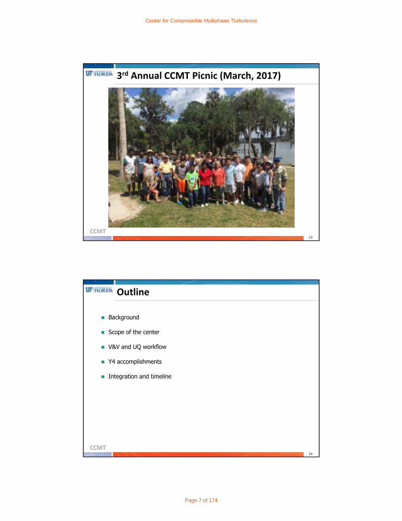
3rd Annual CCMT Picnic (March, 2017)

CCMT14

Outline

Background

Scope of the center

V&V and UQ workflow

Y4 accomplishments

Integration and timeline


Page 7 of 174

CCMT15

Demonstration Problem

CCMT16

PM‐1: Blast Wave Location

PM‐2: Particle Front Location

PM‐3: Number of Instability Waves

PM‐4: Amplitude of Instability Waves

Prediction Metrics


Page 8 of 174

CCMT17

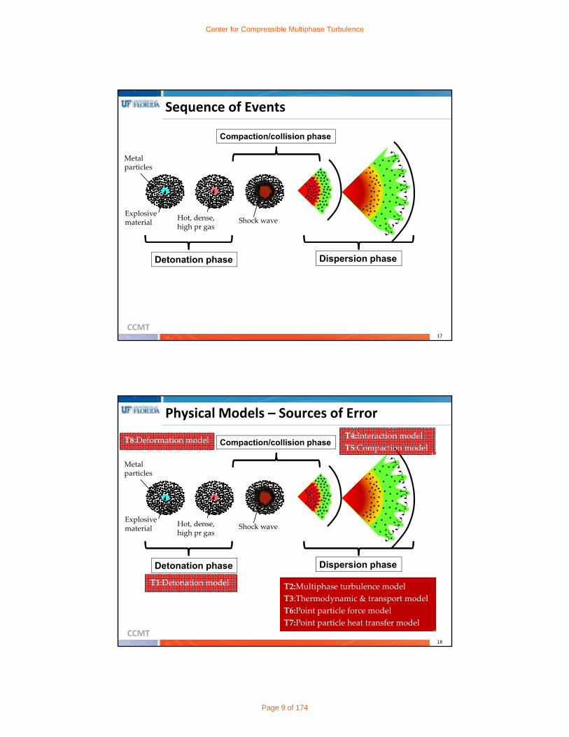
Sequence of Events

Dispersion phaseDetonation phase

Compaction/collision phase

Shock waveHot, dense, high pr gas

Explosive material

Metal particles

CCMT18

Physical Models – Sources of Error



Explosive material

Metal particles

T1:Detonation model

T4:Interaction model

T5:Compaction modelT8:Deformation model

T2:Multiphase turbulence model

T3:Thermodynamic & transport model

T6:Point particle force model

T7:Point particle heat transfer model



Page 9 of 174

CCMT19

Multiscale Integration Strategy

CCMT20

Multiphysics Scope (From Site Visit)

Our focus will be on

– Turbulence at the rapidly expanding material front

– Rayleigh‐Taylor (RT) and Richtmeyer‐Meshkov (RM) instabilities

– Gas‐particle coupling

– Self‐assembly of explosive‐driven particles

Will avoid the following complications

– Free‐shear and wall turbulence (stay away from boundaries)

– Detonation physics (use simple, well‐studied explosives)

– Fragmentation or atomization physics (avoid casing, liquids)

– Reactive physics (use non‐reactive metal particles)


Page 10 of 174

CCMT21

Sources of Errors & Uncertainties

Key Focus

Advance state-of-the-art

- Multiphase turbulence

- Force coupling model

T1: Detonation modeling

T2: Multiphase turbulence modeling

T3: Thermodynamics & transport properties

T4: Particle-particle interaction modeling

T5: Compaction modeling

T6: Force coupling modeling

T7: Thermal coupling modeling

T8: Particle deformation and other complex physics

T9: Discretization and numerical approximation errors

T10: Experimental and measurement errors & uncertainties

CCMT22

Amendment to Scope

Our focus will be on

– Turbulence at the rapidly expanding material front

– Rayleigh‐Taylor (RT) and Richtmeyer‐Meshkov (RM) instabilities

– Gas‐particle coupling

– Self‐assembly of explosive‐driven particles

We have added an intermediate configuration that minimizes

– Compaction effect and associated modeling (T5)

Revised plan includes

– Mesoscale and demonstration experiments with lower

– Use hollow spheres (thin glass beads)


Page 11 of 174

CCMT23

Uncertainty Budget – Overall Plan

T2 – Turbulence modeling

T5 – Compaction modeling

Macroscale

Microscale

Mesoscale

Shock-TubeTrack

ExplosiveTrack

Macroscale U/E QuantificationDiscretizationErrors

ExperimentalError & Uncertainty

ASU MesoscaleExperiments

&Simulations

T2T6 T5

T6

Characterize Particle Bed

Characterize Particle Curtain


Calibration of Explosion

Characterize Particles After

Detonation

Characterization & Calibration

Sandia shock

Experiments&

Simulations

Eglin mesoscale

Experiments&

Simulations

Eglin microscale

Experiments&

Simulations

T4 – Particle interaction modeling

T6 – Force coupling modeling

T4 T4

CCMT24

4 Micro/Meso Campaigns & Target Models

Sandia shock‐tube

– T6: Force coupling and T4: Particle‐particle interaction

ASU expansion fan

– T2: Multiphase turbulence and T4: Particle‐particle interaction

Eglin microscale

– T6: Force coupling

Eglin mesoscale gas‐gun

– T5: Compaction

Demonstration problem

– Yearly hero run


Page 12 of 174

CCMT25

Uncertainty Budget Workflow

Experiments SimulationsExperimental input

Input uncertainty

Target model error

Large?Target model improvement

Computed MetricsMeasured Metrics

Me

asu

rem

ent /

Pre

dic

tion

Control Parameter

Empty Success (Small error, but

Large Uncertainty)

Control Parameter

Useful Failure

Me

asu

rem

ent /

Pre

dic

tion

emodel+eother

emodel+0

CCMT26

Uncertainty Budget Workflow

Experiments Simulations

Propagated uncertainty

Stochastic variability

Discretization error

Neglected feature/physics

Sampling uncertainty

Measurement uncertainty

Measurement processing error

Experimental input

Input uncertainty

Target model error

Large?

Uncertainty

Error

Large?

Target model improvement

Uncertainty/error reduction




Page 13 of 174

CCMT27

UB Workflow ‐ Experiment Worksheet

Experimental input

– Shock properties, particle properties, curtain properties, …

Input uncertainty

– Quantified uncertainties in all the above

Prediction metrics

– PM1: Shock position, PM2: Upstream and downstream curtain

Uncertainty & error quantification (UQ)

– Error in PM1 and PM2 obtained from Schlieren

– Error in X‐ray image particle volume fraction

Uncertainty & error reduction (UR)

– Perform new experiments without spanwise gap

– Improved measurement to reduce volume fraction uncertainty

CCMT28

Hierarchical Error Estimation and UQ

Eglin Macroscale Experiments

Eglin Macroscale Simulations



ASU Mesoscale Simulation

ASU Vertical Shocktube Exp.

T2

T6T4



SNL Mesoscale Simulations

SNL ShocktubeExperiments

T4

T6

T4

T6SNL Mesoscale

Simulations


Eglin Mesoscale Simulations

Eglin Gas gun Experiments

T5T5Eglin Mesoscale

Simulations


VVUU framework

Target modelT?

Eglin Microscale Simulations

Eglin Microscale Experiments



T6T6


Page 14 of 174

CCMT29

Other Simulation Campaigns

Microscale simulations of shock+contact over structured and

random array of particles

– Testing and improvement of force coupling (T6)

Mesoscale simulations of turbulent multiphase jet/plume

– Testing and improvement of multiphase LES (T2)

Mesoscale simulations of sedimentation

– Testing and improvement of particle‐particle interaction model (T4)

Mesoscale simulations of controlled instability

– Evaluation of PM3 and PM4

CCMT30

Y4 Key Accomplishments

Tight integration

Empower students and staff

PIEP model

CMT-nek (O(106) core simulations)

Culture of UQ integration

BE framework and FPGA

Dynamic load balancing


Page 15 of 174

CCMT31

Y4 Highlights

1. Macroscale – Hero Run

2. Blastpad & other validation experiments

3. CMT-nek development and transition

4. Mesoscale – CMT-nek simulation of expansion fan

5. Microscale – Shock + Contact

6. UQ workflow

7. Design space exploration with Behavioral Emulation

8. Dynamic load balancing of Euler-Lagrange

CCMT32

1: Demonstration Problem (Macroscale)

Goal Yearly perform the largest possible

simulations of the demonstration problem and identify improvements to be made in predictive capability

Year 4 Used existing code to perform largescale

simulations of the demonstration problem

Qualitative comparison against experimental data of Frost (PM1 & PM2)

Develop capabilities for the hero runs: real gas EOS, reactive burn, collision modeling

Presentation Bertrand Rollin

3‐D demonstration Simulations


Page 16 of 174

CCMT33

2: Blastpad Experiments

Goals Obtain validation‐quality experimental

measurements of the demonstration problem

Validation‐quality experiments at micro and mesoscales

Perform shock‐tube track micro‐ and mesoscale experiments

Year 4 Blast pad experiments at Eglin AFB

Detailed instrumentation for validation

Simulation informed experiments

Integrated UQ

Presentation Angela Diggs, Bertrand Rollin

ASU

CCMT34

Cam

3

Tungsten Liner Steel Liner

2: Blastpad ExperimentsInput Parameter Source

Explosive length [mm] AFRL measurement

Explosive diameter [mm] AFRL measurement at 5 locations

Explosive density [kg/m3] AFRL calculation

Explosive quality AFRL X-ray

Particle diameter [mm] CCMT measurement

Particle density [kg/m3] CCMT measurement

Particle volume fraction AFRL calculation

Ambient pressure [kPa] AFRL weather station

Ambient temperature [C] AFRL weather station

Probe locations [m] CCMT measurement

SEM of single steel particle at 1000x zoom.

SEM of several steel particles at

100x zoom.


Page 17 of 174

CCMT35

2: Mesoscale Experiments

Goals Obtain validation‐quality experimental

measurements of the demonstration problem

Validation‐quality experiments at micro and mesoscales

Perform shock‐tube track micro‐ and mesoscale experiments

Year 4 Expansion fan experiments at ASU

Detailed instrumentation for validation

Simulation informed experiments

Integrated UQ

Presentation Blair Johnson (ASU)

ASU

CCMT36

3: CMT‐nek Development

Goals Co‐design an exascale code (CMT‐nek) for

compressible multiphase turbulence

Perform micro, meso and demonstration‐scale simulations

Develop & incorporate energy and thermal efficient exascale algorithms

Year 4 Developed and released microscale version

of CMT‐nek for microscale simulations

Developed and released mesoscale version of CMT‐nek for mesoscale simulations

Shock capturing with EVM

CMT‐nek in nek5000 repository

Presentation Jason Hackl and David Zwick

Mach 3, = 1.4,Color Pressure, contour temperature

0 1 2 3 4 5 6 7 8-0.2

0

0.2

0.4

0.6

0.8

t/

CD

Particle Drag

model15%10%3%


Page 18 of 174

CCMT37

3. CMT-nek

Capabilities

– Viscous compressible N-S solver

– DG spectral element (rigorous conservation)

– Shock capturing with EVM

– Spectrally accurate Lagrangian particle solver

– 4-way coupling (Soft-sphere DEM, PIEP)

– Scalable to O(106) cores and more

Class of problems

– Incompressible (Nek-5000) & compressible single phase

– Incompressible & compressible dilute point-particle multiphase

– Incompressible & compressible dense multiphase

CCMT38

4: Mesoscale Simulations

Goal Perform a hierarchy of mesoscale

simulations to allow rigorous validation, uncertainty quantification and propagation to the demonstration problem

Year 4 2‐way coupled simulation with CMT‐nek

Mesoscale simulations of expansion fan over a bed of particles

4‐way coupled simulations with and without PIEP

Bundled simulations for UQ

Presentation David Zwick


Page 19 of 174

CCMT39

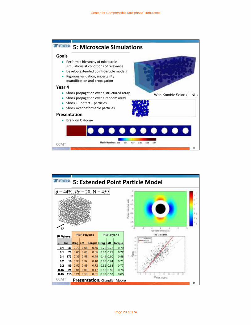
5: Microscale Simulations

Goals Perform a hierarchy of microscale

simulations at conditions of relevance

Develop extended point‐particle models

Rigorous validation, uncertainty quantification and propagation

Year 4 Shock propagation over a structured array

Shock propagation over a random array

Shock + Contact + particles

Shock over deformable particles

Presentation Brandon Osborne

With Kambiz Salari (LLNL)

CCMT40

5: Extended Point Particle Model

Presentation: Chandler Moore

ϕ = 44%, Re = 20, N = 459

U

R2 Values: PIEP-Physics PIEP-Hybrid

ϕ Re Drag Lift Torque Drag Lift Torque

0.1 40 0.70 0.68 0.75 0.72 0.75 0.79

0.1 70 0.65 0.68 0.65 0.67 0.72 0.72

0.1 173 0.35 0.59 0.45 0.44 0.60 0.58

0.2 16 0.38 0.34 0.48 0.66 0.74 0.71

0.2 89 0.50 0.48 0.72 0.62 0.63 0.77

0.45 21 0.01 0.09 0.47 0.55 0.59 0.76

0.45 115 0.21 0.19 0.51 0.63 0.57 0.65

R2 Values: PIEP-Physics

ϕ Re Drag Lift Torque

0.1 40 0.70 0.68 0.75

0.1 70 0.65 0.68 0.65

0.1 173 0.35 0.59 0.45

0.2 16 0.38 0.34 0.48

0.2 89 0.50 0.48 0.72

0.45 21 0.01 0.09 0.47

0.45 115 0.21 0.19 0.51


Page 20 of 174

CCMT41

6: UQ Workflow

Goals Develop UB as the backbone of the Center

Unified application of UB for both physics and exascale emulation

Year 4 Identify main uncertainty sources and quantify

their contributions to the model uncertainty of the shock tube simulation

Reduce uncertainty to focus on model error

UQ and propagation in the context of exascale emulation

JWL mixture‐EOS surrogate for efficient computation

UQ Workflow

Presentation Rafi Haftka, Chanyoung Park, Giselle Fernandez,

Fred Ouellet 0 2 4 6 8

x 10-4

0

0.2

0.4

0.6

0.8

1

Time (Sec)S

ensi

tivity

Inde

x

QSPGAMUVIPHOI

CCMT42

7: Exascale Emulation

Goal Develop behavioral emulation (BE)

methods and tools to support co‐design for algorithmic design‐space exploration and optimization of key CMT‐bone kernels & applications on future Exascale architectures

Year 4 Enhanced BE methods with network

models, interpolation schemes, and benchmarking for CMT‐bone AppBEOs

Performed large‐scale experiments on DOE platforms with BE‐SST simulator

Started design space exploration

Improved throughput and scalability for FPGAs

Presentation Herman Lam, Greg Stitt, Sai Chenna


Page 21 of 174

CCMT43

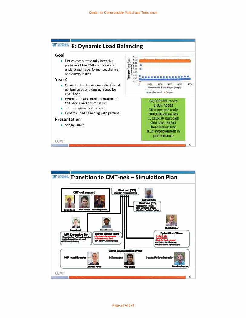
8: Dynamic Load Balancing

Goal Derive computationally intensive

portions of the CMT‐nek code and understand its performance, thermal and energy issues

Year 4 Carried out extensive investigation of

performance and energy issues for CMT‐bone

Hybrid CPU‐GPU implementation of CMT‐bone and optimization

Thermal aware optimization

Dynamic load balancing with particles

Presentation Sanjay Ranka

CCMT44

Transition to CMT‐nek – Simulation Plan


Page 22 of 174

CCMT45

Transition to CMT‐nek – CCMT Workshop

Agenda• CMT-nek: Anatomy of the Beast

Speaker: Jason Hackl | 12:00 pm – 1:30 pm

• Lagrangian Particles in CMT-nekSpeaker: David Zwick | 1:30 pm – 2:30 pm

• Running CMT-nekSpeakers: Goran Marjanovic and Brad Durant | 2:30 pm – 3:15 pm

• Post-Processing and visualization in CMT-nekSpeakers: David Zwick and Brad Durant | 3:15 pm – 4:00 pm

• Lesson Learnt from CCMT’s SimulationsSpearkers: Fred Ouellet and Yash Mehta | 4:00 pm – 5:00 pm

Attendee listPaul CrittendenBrad DurantGiselle FernandezJoshua GarnoJason HacklRahul KoneruYash MehtaGoran MarjanovicChandler MooreFred Ouellet Brandon OsborneBertrand RollinPrashanth SridharanDavid Zwick

A Boot Camp on CMT-nekNovember 29, 2017

Organizers: Bertrand Rollin, Jason Hackl

CCMT46

Transition to CMT‐nek – Timeline

Task Year4 Year5

NOV DEC JAN FEBMAR

APR MAY JUN JUL AUG SEP OCT NOV DEC JAN FEBMAR

APR

Training with CMT-nek W

Blastpad Simulation 3D (Hero Run)

Eglin Mesoscale Experiment (2D)


Eglin Microscale Experiment (2D)


Sandia Shock Tube Experiment

ASU Expansion Fan

W Workshop: "A Boot Camp on CMT-nek"


Page 23 of 174

CCMT47

CMT‐nek – Blastpad Hero Runs

Hero Run 6 Hero Run 7 Hero Run 8

Reactive burn No No Yes

Equation of state Ideal Gas JWL JWL

Initial Particle volume fraction 5 % 10 % 60 %

Particle bed perturbation none 1 mode – (Notched Case) Random

No. of computational particles 20 B 20 B 20 B

No. of Grid Points1.8 B

(1,025,000 Spectral Elements, 12x12x12 grid points/element)

1.8 B(1,025,000 Spectral Elements, 12x12x12 grid points/element)

14 B(8,200,000 Spectral Elements, 12x12x12 grid points/element)

No. of cores 131K 131K 393,216(All of Vulcan - DAT)

Simulation Time 0.5ms 3.0ms 6.0ms

CCMT48








T2

T6T4





T4

T6

T4

T6SNL Mesoscale

Simulations




T5T5Eglin Mesoscale

Simulations


VVUU framework

Target modelT?





T6T6

Model error estimation and UQ of T6 and T4 will be com by Y4Q4 UQ of the particle curtain model is being carried out


Page 24 of 174

CCMT49








T2

T6T4





T4

T6

T4

T6SNL Mesoscale

Simulations




T5T5Eglin Mesoscale

Simulations


VVUU framework

Target modelT?





T6T6

Model error estimation and UQ of T6 (Y5Q2) Finished the experiments (Y2Q2) Complete interventional UQ of the experiments

(Y5Q1) Complete microscale simulation (Y5Q1) Quantify numerical error (Y4Q4)

CCMT50








T2

T6T4





T4

T6

T4

T6SNL Mesoscale

Simulations




T5T5Eglin Mesoscale

Simulations


VVUU framework

Target modelT?





T6T6

Model error estimation and UQ of T2 and T4 will be finished by Y5Q4 Plan for validating the turbulence model T2 (Y5Q1) Complete a simulation with the turbulence model into

CMT-nek (Y5Q3) Quantify numerical error of the turbulence model (Y5Q4) Prepare experiment plan for measuring prediction metrics

(Y6Q1) Complete the planned experiments (Y6Q2) Complete interventional UQ of the experiments (Y6Q3)


Page 25 of 174

CCMT51








T2

T6T4





T4

T6

T4

T6SNL Mesoscale

Simulations




T5T5Eglin Mesoscale

Simulations


VVUU framework

Target modelT?





T6T6

Model rror estimation and UQ of T5 (Y5Q4) Finished the experiments (Y4Q3) Complete interventional UQ of the experiments (Y5Q1) Complete mesoscale simulation (Y5Q2) Quantify numerical error (Y5Q2)

CCMT52








T2

T6T4





T4

T6

T4

T6SNL Mesoscale

Simulations




T5T5Eglin Mesoscale

Simulations


VVUU framework

Target modelT?





T6T6

Prediction error estimation and UQ of demonstration simulation (Y6Q4) Complete Eglin Blast pad experiments (Y5Q4) Complete interventional UQ of the experiments (Y6Q1) Complete lower fidelity simulation(s) for UQ with

multi-fidelity surrogate (Y5Q1) Quantify numerical error of the lower fidelity

simulation (Y5Q1) Complete hero simulations (Y5Q4) Quantify numerical error of hero simulation (Y5Q4)


Page 26 of 174

CCMT53

Timeline

CCMT

CCMT

Do you have any questions?


Page 27 of 174

CCMT

CCMT

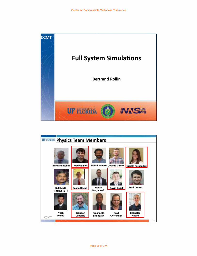
Full System Simulations

Bertrand Rollin

CCMT

Physics Team Members

| 2

Fred OuelletBertrand Rollin Rahul Koneru Joshua Garno Giselle Fernandez

Brad Durant Jason Hackl

PaulCrittenden

GoranMarjanovic

YashMehta

BrandonOsborne

PrashanthSridharan

SiddharthThakur (ST)

David Zwick

Chandler Moore


Page 28 of 174

CCMT

Bring predictive capabilities to particle-laden flow simulations under extreme conditions

Explosive‐Driven Particle‐Laden Flows

| 3

CCMT

Outline

Demonstration Problems Frost’s Experiment Eglin’s Blastpad Experiment

Micro and Mesoscale Campaigns Eglin Microscale Experiments Eglin Mesoscale Experiments SNL’s Multiphase Shock Tube ASU Expansion Fan

| 4


Page 29 of 174

CCMT

Physical Models – Sources of Error




Explosive material

Metal particles

T1:Detonation model

T4:Collision model

T5:Compaction modelT8:Deformation model

T2:Multiphase turbulence model

T3:Thermodynamic & transport model

T6:Point particle force model

T7:Point particle heat transfer model

| 5

CCMT

Hero Runs

| 6

• 60 Million computational cells• 15 Million computational particles• rmax = 4.00m• tmax = 1.40ms• 5760 cores

Features:• 30 Million computational cells• 5 Million computational particles• rmax = 4.00m• tmax = 2.50ms• 4096 cores

HR 2 HR 3


Page 30 of 174

CCMT

Hero Run: Evolution

| 7

Hero Run 1

Hero Run 2

Hero Run 3

Hero Run 4A

Hero Run 4B

Hero Run 5

Reactive burn No No Yes Yes Yes Yes

Equation of state Ideal Gas JWL JWL JWL JWL JWL

Initial Particle volume fraction

5 % 40 % -Frozen

10 % -Frozen

10 % -Frozen

10 % -Frozen

10 % -Frozen

Particle bed perturbation

none none 1 mode in azimuthaldirection

none 4 mode in azimuthaldirection+ white noise

none

No. of computational

particles

5 M 5 M 15 M 15 M 15 M 30 M

No. of elements 30 M 30 M 60 M 60 M 60 M 120 M

No. of cores 512 4096 5760 5760 5760 16384

Simulation Time 2.5ms 2.5ms 1.40ms 0.20ms 0.42ms 0.03ms

currently running

CCMT

Hero Run 3: Reactive Burn Initial Conditions

| 8


Page 31 of 174

CCMT

Hero Run 3: Equation of State Model

| 9

The Jones-Wilkins-Lee (JWL) equations of state are used to predict the pressures of high energy substances and are:

where and , , , , , and are parameters for the substance.

Iterative method One EquationMulti‐fidelity Surrogate

Advantage

‐ Accuracy‐ Problem

independent

‐ Speed‐ Algebraic

equation

‐ Speed‐ Take account of

species equation

Disadvantage

‐ May be slow to converge

‐ Computationally expensive

‐ Uncertainty and error

‐ JWL + ideal gas case only

‐ Uncertainty‐ Equation of State

specific (problem specific)

“EoS Surrogate Modeling”, Fred Ouellet

CCMT

Demonstration Problem: Predictions

Blast Wave Location (PM-1)

| 10


Page 32 of 174

CCMT

Demonstration Problem: Predictions

Particle Front Location (PM-2)

| 11

CCMT

Hero Run 3 – A Closer Look

| 12


Page 33 of 174

CCMT

Hero Run 3 – A Closer Look

“Multi-fidelity surrogate model for finding the fastest growing initial perturbation ”, M. Giselle Fernandez-Godino

| 13

t=0, k=24

t=168µsDominant modes k=24 and k=48

t=480µsNo dominant modes

t=962µsk=24 emerging again

CCMT

Outline



| 14


Page 34 of 174

CCMT| 15

AFRL Blastpad Experimental Setup Instrumentation:

54 pressure probes Momentum traps (instrumented

possible) Four high speed video cameras Linear optical transducers

Six shots 2 bare charges 1 charge w/tungsten (notched) 1 charge w/steel (notched) 2 charges w/steel (un-notched)

Locations of 54 pressure transducers (Barreto et al. 2015).

Picture of charge suspended before a test

(Barreto et al. 2015)

Distribution A. Approved for public release. Distribution unlimited.

“Eglin Experiment”, Angela Diggs

CCMT

Blastpad Simulation (Bare charge 1d results)

| 16

1D Simulation Details:• 100,000 cells in radial direction up to 6 m.• Run using 16 cores up to a time of 4.5 ms• 1 Equation JWL Model for Composition-B used for EoS


Page 35 of 174

CCMT

Blastpad Simulation Setup

| 17

Preliminary Simulation Details:• 1 million cells in two dimensions• To be run on 256 cores using LLNL’s Quartz machine• Exhaust boundary is an outflow• Other bottom boundaries are slipwalls• 4 probes set in locations of experimental sensors• 40 other probes set in near-charge region

Note: Bare charge setup is shown, particles will be included in parallel runs

CCMT

Outline



| 18


Page 36 of 174

CCMT| 19

Eglin’s Experiments

CCMT Sample x-ray.

Eglin’s Experiments

Centerline

44.45

PBXN-5

120

Positions captured by x-rays

38.1 25.4

Steel

76.2

Particle6.35

| 20

Simulations implement the JWL equation of state and reactive burn initial condition for the explosive

Plan for Uncertainty Quantification Analysis▪ Vary input parameters of particle density, particle diameter, and explosive mass for batch run

(5 x 5 x 5 x 3 simulations) to construct surrogate model▪ Done for all variations of particle configuration

Current geometry has a solid backwall for the explosive▪ In reality there is a sizable hole in the back of the explosive where the detonator attaches▪ Simulations will compare the effects of including this hole


Page 37 of 174

CCMT

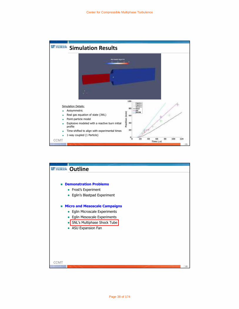
Simulation Results

Simulation Details:■ Axisymmetric■ Real gas equation of state (JWL)■ Point-particle model■ Explosive modeled with a reactive burn initial

profile■ Time-shifted to align with experimental times■ 1-way coupled (1 Particle)

| 21

CCMT

Outline



| 22


Page 38 of 174

CCMT| 23

New Particle Curtain Experiments

Curtain thickness after impact

No Side Gaps

CCMT| 24

Large‐Scale Bundle Runs

Comparison between mesoscale 1D/2D/3D simulations and the new SNL experiments with non-tophat initial particle volume fraction profile Runs for:

5 different Mach numbers: 1.24, 1.40, 1.45, 1.66, 1.92 Initial particle volume fraction Random initial particle locations Curtain thickness

625 1D bundle runs with Dakota 135 2D runs 27 3D runs

“Uncertainty Budget”, Chanyoung Park


Page 39 of 174

CCMT| 25

3D Particle Curtain Simulation

• 18 Million computational cells• 6 Million computational particles• 2048 cores

Features:

X-Y Plane

Y-Z Plane

CCMT| 26

Shock Tube Results

• Particle fronts are defined as the locations of the trailing and leading 0.5% of particles

“Uncertainty Budget”, Chanyoung Park


Page 40 of 174

CCMT

Outline



| 27

CCMT

ASU Experiment•Simulations are progressing with CMT‐nek

“CMT-nek”, Jason Hackl and David Zwick

| 28

“ASU Experiments”, Blair Johnson


Page 41 of 174

CCMT

CCMTDo you have any

questions?

Eglin Blast Pad simulation by CMT-nek


Page 42 of 174

CCMT

CCMT

CMT-nek Development

and Application

Jason Hackl

David Zwick

CCMT2

CMT‐nek development team

Prof. Paul Fischer, UIUC

Li Lu,UIUC

Jason Hackl, UF

David Zwick, UF

Goran Marjanovic, UF

BradDurant

Brad Durant,UF

Rahul Koneru,UF

Postdoctoral fellow Nguyen Tri Nguyen arrives December 10th, 2017


Page 43 of 174

CCMT3

Outline

CMT‐nek hydrodynamics

― Discontinuous Galerkin spectral element method

― Euler equations + entropy viscosity method (EVM)

Microscale release

― Shock waves and interactions of waves with spheres

CMT‐nek particles

― Multiphase source terms

― Algorithms and parallelization

Mesoscale release

― ASU experiment

CCMT4

Discontinuous Galerkin SEM

Ronquist and Patera (1987) Intl. J. Numerical Methods Engrg. 24, 2273-2299Deville, Fischer and Mund (2002) Higher-Order Methods for Incomp. Flows CambridgeDolejší & Feistauer(2015) Discontinuous Galerkin Method:Analysis & Applications to Compressible Flow. Springer

ith variable’s flux = convective + diffusive

1. Inner product with test function v2. Integrate by parts on hexahedral Ωe

3. Numerical flux H* in surface integral• Weak boundary conditions• Couples elements together

4. Isoparametrically map Ωe to [-1,1]d

5. Approximate integrals with quadrature6. Approximate U & v with Lagrange polynomials

• N Gauss-Legendre-Lobatto (GLL) nodes• Nested tensor product ~ O(N4) < N3 x N3

N x N matrices applied N2 times

Matrix opswithin Ωe


Page 44 of 174

CCMT5

Thermodynamic stateTemperaturePressureTotal energy

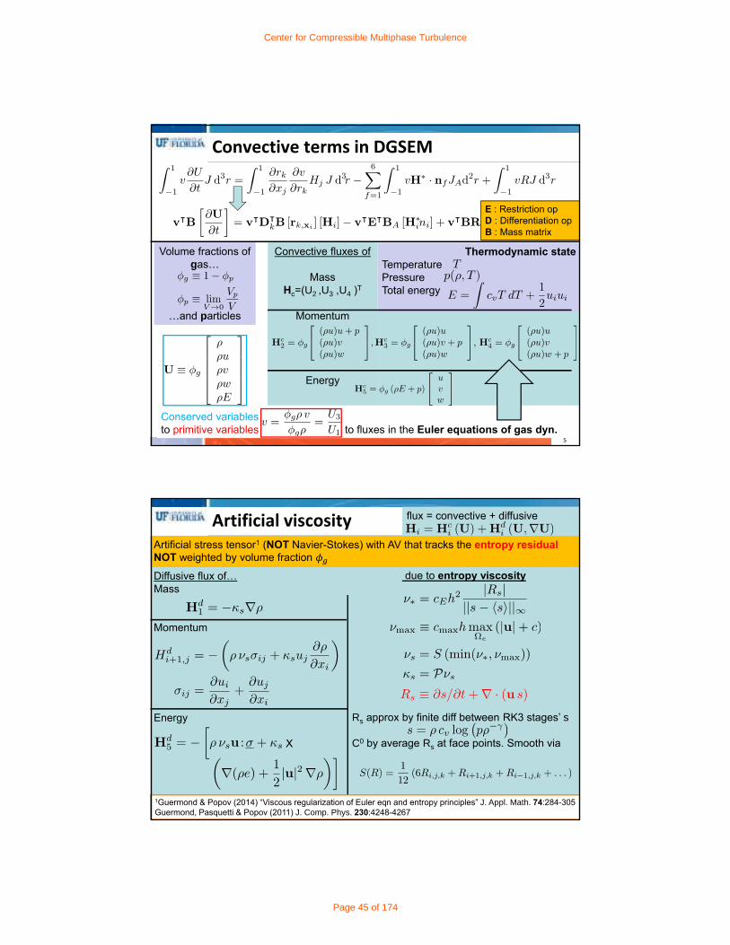
Convective terms in DGSEM

Volume fractions of gas…

…and particles

Convective fluxes of

MassHc=(U2 ,U3 ,U4 )T

Momentum

Energy

Conserved variablesto primitive variables to fluxes in the Euler equations of gas dyn.

E : Restriction opD : Differentiation opB : Mass matrix

CCMT6

flux = convective + diffusiveArtificial viscosity

Diffusive flux of…Mass

Mass

Momentum

Energy

X

due to entropy viscosity

Rs approx by finite diff between RK3 stages’ s

C0 by average Rs at face points. Smooth via

1Guermond & Popov (2014) “Viscous regularization of Euler eqn and entropy principles” J. Appl. Math. 74:284-305Guermond, Pasquetti & Popov (2011) J. Comp. Phys. 230:4248-4267

Artificial stress tensor1 (NOT Navier-Stokes) with AV that tracks the entropy residualNOT weighted by volume fraction


Page 45 of 174

CCMT7

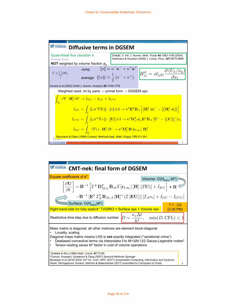
Diffusive terms in DGSEM

Baumann & Oden (1999) Comput. Methods Appl. Math. Engrg. 175:311-341

Quasi-linear flux Jacobian APrimal formNOT weighted by volume fraction

Jump

average

Dolejší, V. Intl. J. Numer. Meth. Fluids 45:1083-1106 (2004)Hartmann & Houston (2008) J. Comp. Phys. 227:9670-9685

Arnold et al (2002) SIAM J. Numer. Analysis 39:1749-1779

Weighted resid, int by parts → primal form → DGSEM ops

CCMT8

CMT‐nek: final form of DGSEM

Right-hand-side for fully explicit1 TVDRK3 = Surface ops + Volume ops

Equate coefficients of vT

Volume: O(Nelem M4)

Surface: O(NelemM2)

Mass matrix is diagonal; all other matrices are element block-diagonal• Locality, scalingDiagonal mass matrix means LHS is not exactly integrated (“variational crime”)• Dealiased convective terms via interpolator I to M=3(N-1)/2 Gauss-Legendre nodes2

• Tensor-nesting saves M2 factor in cost of volume operations

+ R

Restrictive time step due to diffusion number

T 7 : CS(2:30 PM)

1Gottlieb & Shu (1998) Math. Comp. 67:73-852Canuto, Hussaini, Quateroni & Zang (2007) Spectral Methods SpringerBanerjee et al (2016) IEEE 23rd Int. Conf. HiPC (2017) Sustainable Computing, Informatics and SystemsHackl, Shringarpure, Koneru, Delchini & Balachandar (2017) submitted to Computers & Fluids


Page 46 of 174

CCMT| 9

Shock capturing in CMT‐nek

1Sod (1978) J. Comp. Phys. 27:1-312Shu & Osher (1989) J. Comp. Phys. 83:32-783Lv, See & Ihme (2016) J. Comp. Phys. 322:448-472

Calibrated P, cE, cmax in Sod1 shock tube

• * reaches max at shock wave• Less oscillatory than other HODG3

h = 0.01, N = 9, t =0.02

Shu-Osher2 1D shock-turbulence surrogate

h = 0.01, N = 5, t =0.02

CCMT| 10

CMT‐nek convergence and validationHomentropic vortex: exponential convergence in smooth flow

h0.996

N -1.08

N = 5

N = 7

N = 9

N - 1

N = 9

h = 0.01

Two-shock collision, t = 0.035: O(1) Empirical order of convergence in h & p


Page 47 of 174

CCMT| 11

Microscale: Potential flow over spheresTests generalized Faxen theorem1

FCC 15% Volume fraction

FCC 10% Volume fraction

1Annamalai & Balachandar (2017) J. Fluid. Mech. 816, 381-411

0 1 2 3 4 5 6 7 8-0.2

0

0.2

0.4

0.6

0.8

t/

CD

Particle Drag

model15%10%3%

Nelem 23424

Spheres 95

Rows 21

CMT-nek supports model dev

CCMT| 12

Microscale: Mach 3 shock‐sphere• 220 - element mesh from GridPro, far-field h=0.1075dp

• N = 5, 125M DOF in surrounding 10dp x 10dp x 10dp box• 8192 cores on Vulcan

cE cmax P ∆t

40 0.5 0.75 2.5e-6


Page 48 of 174

CCMT| 13

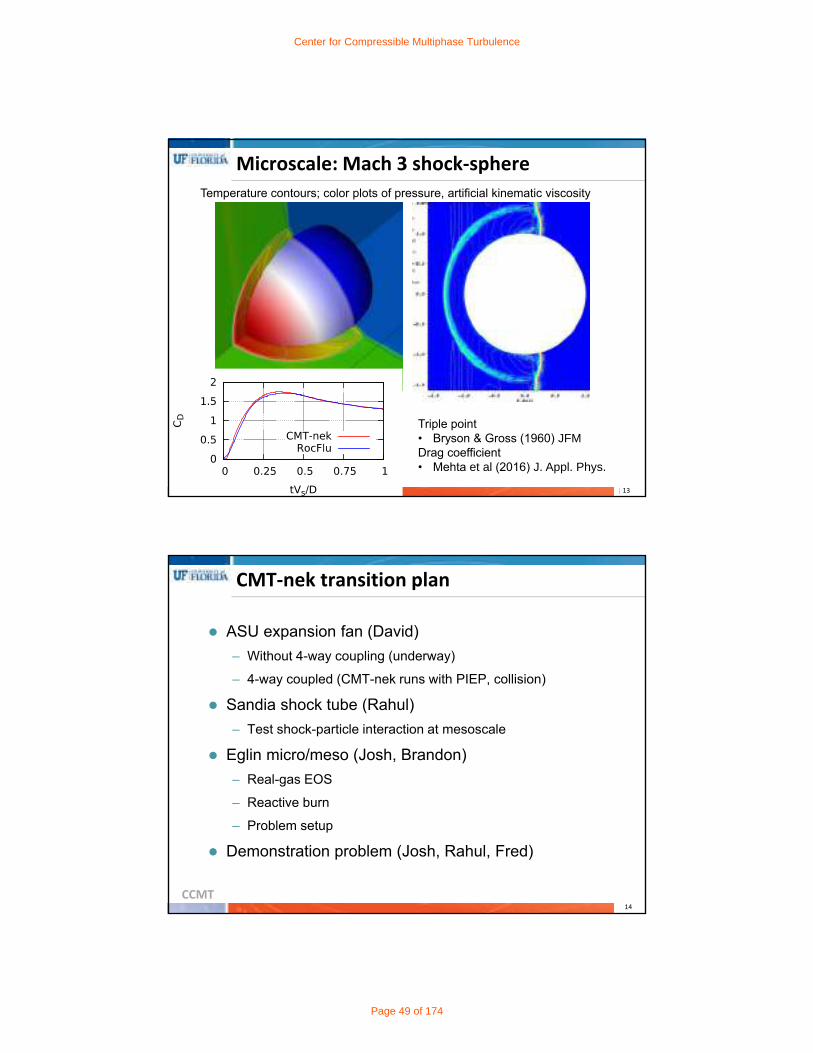
Microscale: Mach 3 shock‐sphere

Temperature contours; color plots of pressure, artificial kinematic viscosity

Triple point • Bryson & Gross (1960) JFMDrag coefficient• Mehta et al (2016) J. Appl. Phys.

CCMT14

CMT‐nek transition plan

ASU expansion fan (David)

– Without 4-way coupling (underway)

– 4-way coupled (CMT-nek runs with PIEP, collision)

Sandia shock tube (Rahul)

– Test shock-particle interaction at mesoscale

Eglin micro/meso (Josh, Brandon)

– Real-gas EOS

– Reactive burn

– Problem setup

Demonstration problem (Josh, Rahul, Fred)


Page 49 of 174

CCMT15

Transition to CMT‐nek – Timeline

Task Year4 Year5

NOV DEC JAN FEBMAR

APR MAY JUN JUL AUG SEP OCT NOV DEC JAN FEBMAR

APR

Training with CMT-nek W

Blastpad Simulation 3D (Hero Run)





Sandia Shock Tube Experiment

ASU Expansion Fan

W Workshop: "A Boot Camp on CMT-nek"

CCMT16

Transition to CMT‐nek – CCMT Workshop

Agenda• CMT-nek: Anatomy of the Beast

Speaker: Jason Hackl | 12:00 pm – 1:30 pm

• Lagrangian Particles in CMT-nekSpeaker: David Zwick | 1:30 pm – 2:30 pm

• Running CMT-nekSpeakers: Goran Marjanovic and Brad Durant | 2:30 pm – 3:15 pm

• Post-Processing and visualization in CMT-nekSpeakers: David Zwick and Brad Durant | 3:15 pm – 4:00 pm

• Lesson Learnt from CCMT’s SimulationsSpearkers: Fred Ouellet and Yash Mehta | 4:00 pm – 5:00 pm

Attendee listPaul CrittendenBrad DurantGiselle FernandezJoshua GarnoJason HacklRahul KoneruYash MehtaGoran MarjanovicChandler MooreFred Ouellet Brandon OsborneBertrand RollinPrashanth SridharanDavid Zwick

A Boot Camp on CMT-nekNovember 29, 2017

Organizers: Bertrand Rollin, Jason Hackl


Page 50 of 174

CCMT17

Multiphase Flow in CMT‐nek

CMT-nek is built on single-phase nek5000

While not fully resolved, Eulerian-Lagrangian method can simulate a realistic (~109) particles

Difficulties related to particle-fluid coupling

– Physics

– Numerics

– Computer Science

Outline

– Particle implementation in CMT-nek/nek5000

– ASU experiment application

CCMT18

Multiphase Source Terms

Particle-fluid force coupling and energy contribution

Particle-fluid energy coupling Eulerian particle velocity

Lagrangian to Eulerian Transfer

y

x

Reference Frames


Page 51 of 174

CCMT19

Dispersed Phase

Position:

Momentum:

Energy:

• For a single particle:V

x

y

z

X

u,Tf,p,ρf

Hydrodynamic force Collisional force

Body force Hydrodynamic heat transfer

Tp

Mp

CCMT20

Interpolation

• Fluid properties need to be evaluated at particle location

• Quasi-steady force:

• Interpolation choices:Method Accuracy Scalability

Linear O(1/N2) O(1) – O(N)

Cubic O(1/N4) O(N) – O(N2)

Lagrange O(1/NN+1) O(N6)

Barycentric Lagrange O(1/NN+1) O(N3)

N+1 grid points


Page 52 of 174

CCMT21

Projection

• Process of spreading Lagrangian quantities to the Eulerian reference frame

• Arises from volume filtering used to get multiphase governing equations

• Here, a Gaussian filter is used

A (Lagrangian) a (Eulerian)-Fpg fpg

-Gpg gpg

-Qpg qpg

Vp Φp

VpV Φpv

CCMT22

Ghost Particles

Idea: If a particle is near a MPI rank edge, it will create a

copy of itself called a ghost particle Sending perspective rather than receiving perspective

MPI Rank 0 MPI Rank 1

MPI Rank 2 MPI Rank 3

send

send

send

Rank 0 Rank 1

Rank 2 Rank 3

After GP Transfer

GP steps:1. Create GP2. Send GP(Ghost particles shown in orange boxes)


Page 53 of 174

CCMT23

Algorithmic Scaling

Ideal Setup: Uniform flow in a periodic box Particle time scale is 10 time steps One particle per grid point N = 5 grid points in each direction Vulcan (LLNL) CS Team will show load-imbalanced casesStrong Scaling: 13 million grid points 13 million particles

Weak Scaling: 6,250 grid points/rank 6,250 particles/rank

Time is averaged over MPI ranks and time steps

CCMT24

Algorithmic Scaling

Strong scaling diverges from ideal due to: 1 element/rank Ghost particles

Weak scaling diverges from ideal due to: Inter-processor communication from sending particles

Weak Scaling(without GP Comm.)

Example Profiling(10,000 rank case from strong scaling)


Page 54 of 174

CCMT25

Particles in Expansion Waves

• Simulation of vertical shock tube with particle bed at bottom

• When diaphragm bursts, particle bed will swell upwards

• ASU team will provide more detail

• Main goals:1. Uncertainty study

2. Physics

3. High resolution

Joints

High Speed Camera

CCMT26

Shock tube (no particles)

Prediction (Validation) Metrics

Shock tube with particles

Prediction metrics:

• Bed height

• Fluid pressure


Page 55 of 174

CCMT27

Detailed Simulation


0.64 5.76

0.64 0.64

0.04 0.04

-0.3 -0.3


5 5

294 294

101 101

294 294

40% 40%


[44,88] [44,88]

kg/ ] 2,460 2,460

5,033,861,327 229,500

Geometry Particles

Initial ConditionsSimulations

20,000

800

, 5

6

Δ 0.0013

/Δ 2.5

/ [38,76]

Ranks 8,192

Grid

CCMT28

Initial Results

Experimental Tube Joint (x = -32 cm)

Initial Bed Height(x = -30 cm)


Page 56 of 174

CCMT29

Planar Averaged Profiles

Initial Bed Height(x = -30 cm)

Observations:

• Reflected/transmitted expansion wave when incident expansion wave head hits bed

• Pressure ahead of bed is nearly constant but lower than standard shock tube

• Possible clustering of particles

CCMT30

Bed Height

Planar Averaging

Box Filter

Threshold

1% of


Page 57 of 174

CCMT31

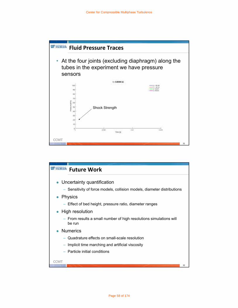
Fluid Pressure Traces

• At the four joints (excluding diaphragm) along the tubes in the experiment we have pressure sensors

Shock Strength

CCMT32

Future Work

Uncertainty quantification

– Sensitivity of force models, collision models, diameter distributions

Physics

– Effect of bed height, pressure ratio, diameter ranges

High resolution

– From results a small number of high resolutions simulations will be run

Numerics

– Quadrature effects on small-scale resolution

– Implicit time marching and artificial viscosity

– Particle initial conditions


Page 58 of 174

CCMT

CCMT


CCMT34

High Resolution Simulation


0.64 5.76

0.64 0.64

0.04 0.04

-0.3 -0.3


5 5

294 294

101 101

294 294

40% 40%


[44,88] [44,88]

kg/ ] 2,460 2,460

5,033,861,327 73,440,000

Geometry Particles

Initial ConditionsSimulations

1,280,000

3,200

, 20

6

Δ 0.0003

Ranks 131,072

Grid


Page 59 of 174

CCMT35

Uncertainty Quantification

• Full factorial design

Configuration Force Model

1

2

3

Configuration Collision Model

1 Off

2 Walls Only

3 Particles Only

4 Walls & Particles

Configuration Diameter Distribution

1 Monodisperse

2 Polydisperse

• Soft-sphere collision model

• 72 total simulations (3 repeats)

CCMT36

Physics Simulations

• Full factorial design

Configuration Bed Height

1 -30 cm

2 −20 cm

3 −10 cm

4 0 cm

Configuration Pressure Ratio

1 5

2 10

3 20

4 40

Configuration Diameter Range

1 [44,88]

2 [89,149]

• Parameters chosen to compare to experiments:

– ASU

– Literature (Chojnicki et al., 2006)

• 96 total simulations(3 repeats)


Page 60 of 174

CCMT

CCMT

Experimental Studies of Gas‐Particle Mixtures

Under Sudden Expansion

Blair Johnson, Ph.D., Heather Zunino

Ronald Adrian, Ph.D., Amanda Clarke, Ph.D.

Arizona State University

CCMT2

Outline

Research Objectives

Experimental Setup & Measurement Techniques Installation of new pressure sensors

Synchronization to optical measurements

High speed video of particle bed evolution

Particle image velocimetry (PIV) of gas

Results Pressure analysis

Particle bed motion

Gas velocity

Summary & Upcoming Work


Page 61 of 174

CCMT3

Research Objectives

Provide data for validation of numerical simulations

developed by CCMT.

Measure shock wave, expansion wave, incipient

particle bed motion and gas flow, and particle motion

in 0 < z < D (near field), 0 < z < 7D (far field),and

z < 0 (within bed).

Coordinate with UQ, UB teams to quantify

experimental error and gain insight for potential

improvements to experimental facility.

CCMT4

Experimental Plan

Particle size (μm)

Pressure RatioP4 / P1

Bed Height (cm)

MeasurementType

# of tests

44 – 90 20 37.9 FV 10

32+ EXP ∞

10.0 PIV ∞

15 37.9 FV 2

10 37.9 FV 2

90 – 150 20 37.9 FV 2

32+ EXP ∞

15 37.9 FV 2

10 37.9 FV 2

150+ 20 10.0 PIV ∞

FV = Front Rise VelocityEXP = Bed Expansion Video of Crack/Void EvolutionPIV = Particle Image Velocimetry for gas velocity


Page 62 of 174

CCMT5

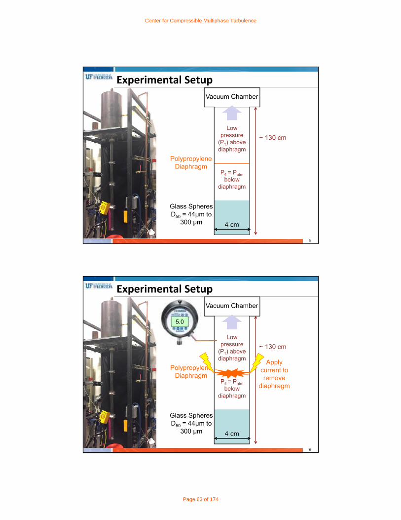
Experimental Setup

Vacuum Chamber

~ 130 cm

Polypropylene Diaphragm

Glass Spheres D50 = 44μm to

300 μm 4 cm

P4 = Patm

below diaphragm

Low pressure

(P1) above diaphragm

CCMT6

Experimental Setup

Vacuum Chamber

Polypropylene Diaphragm


300 μm 4 cm

P4 = Patm

below diaphragm

Low pressure


~ 130 cm

5.0

Apply current to remove

diaphragm


Page 63 of 174

CCMT7

Experimental Setup

Vacuum Chamber


300 μm 4 cm

P4 = Patm

below diaphragm

Low pressure


5.0

Shock

Rarefaction Wave

Pressure Sensors

(200 kHz)

~ 130 cm

CCMT8

Experimental Setup

Vacuum Chamber


300 μm 4 cm

5.0

Shock

Rarefaction Wave

Pressure Sensors

(200 kHz)

Phantom v641 4-megapixel high

speed camera (Fs = 10,000+ fps)

P4 = Patm

below diaphragm

Low pressure



Page 64 of 174

CCMT9

Experimental Setup

Vacuum Chamber

Shock

Rarefaction Wave

Pressure Sensors

(200 kHz)



Expansion of particle

bed

Escape/rise of

interstitial gas

CCMT10

Experimental Setup

Vacuum Chamber

Shock

Rarefaction Wave

Pressure Sensors

(200 kHz)




Page 65 of 174

CCMT11

Measurement Techniques

Pressure sensors

High-speed (10 kfps) video

Particle bed expansion

Front velocity

Particle image velocimetry (PIV) of gas in expansion

region at top of particle bed

CCMT12

Dynamic Pressure Sensors

5.0

• Static pressure sensor Omega DPG9145-15pressure above diaphragm (below ~ atmospheric)

• Holes built into diaphragm joint ensure P4 = Patm


Page 66 of 174

CCMT13


118o

59o

5.0


• Dynamic sensors PCB113B28, Fs = 200 kHz

• Use shock to trigger/sync optical measurements

• Detect lateral variations of shock and expansion waves (UQ, simulation)

CCMT14


118o

59o

5.0


• Dynamic sensors PCB113B28, Fs = 200 kHz

• Use shock to trigger/sync optical measurements

• Detect lateral variations of shock and expansion waves (UQ, simulation)


Page 67 of 174

CCMT15

Pressure Sensors / Synchronization

8 pressure sensors (PCB 113B28) read simultaneously into LabView via PXIe-4492

Pressure threshold set in LabView (UQ, simulation) Shock trigger for particle bed measurements Expansion trigger for gas PIV

CCMT16

Pressure Sensors / Synchronization

Hardware trigger sent from PXIe-4492 to PXIe-6341, to BNC-2120, to BNC 565 pulse/delay generator, and to Phantom v641 camera

Trigger received by camera to initiate optical recording


Page 68 of 174

CCMT17

High speed video

Left: Bed rise

Right: Void development

Fs = 10,000 fps

CCMT18

Particle Image Velocimetry (PIV)

Image 1 Image 2Δt = 80 μs


Page 69 of 174

CCMT19


Image 2

Image 1

CCMT20



Page 70 of 174

CCMT21


Vacuum Chamber

10 cm

32 cm

Gas velocity above particle bed, within interstices in top layers of particle bed

10 μm silver-coated hollow glass spheres

Seeded at top of bed, injected above bed

Double-pulsed Nd:YAG laser

CCMT22


Vacuum Chamber

10 cm

Pressure Sensors

(200 kHz)

32 cm






Page 71 of 174

CCMT23


Vacuum Chamber

10 cm

Pressure Sensors

(200 kHz)

32 cm




Triggered in expansion

Synchronization via BNC 565 pulse/delay generator


CCMT24


Vacuum Chamber

10 cm

Pressure Sensors

(200 kHz)

32 cm

Field of view: 4 cm x 4 cm, above 10cm bed

Δt ~ 80 μs

Fs = 14 Hz (limited by laser)



Page 72 of 174

CCMT25


Vacuum Chamber

10 cm

Pressure Sensors

(200 kHz)

32 cm

Field of view: 4 cm x 4 cm, above 10cm bed

Δt ~ 80 μs

Fs = 14 Hz (limited by laser)


CCMT26


Vacuum Chamber

10 cm

Pressure Sensors

(200 kHz)

32 cm

Fs = 14 Hz Adjust time delay between expansion wave trigger and initiation of PIV

Explore repeatability based on delay time (UQ)

Build spatio-temporal record of velocity fields



Page 73 of 174

CCMT27

Outline

Research Objectives






Particle bed motion

Gas velocity


CCMT28

Results – Pressure Sensors


Page 74 of 174

CCMT29


CCMT30

Results – Wave Speeds

Vshock ~ 500 m/s

Vexp ~ 12 m/s(through particle bed)


Page 75 of 174

CCMT31

Results – Flatness of Shock

CCMT32



Page 76 of 174

CCMT33

Results – Pressure Sensorst = -0.0005 s

CCMT34

Results – Particle Bed Front Velocity

• P4/P1 = 20; P1 ~ 5 kPa• Track bed height as a function of time,

~60% intensity• Cubic fit to experimental data


Page 77 of 174

CCMT35

Results – Particle Bed Front Velocity

• P4/P1 = 20; P1 ~ 5 kPa

• 8 experiments of identical conditions

CCMT36

Results – Particle Bed Packing

• Able to measure mass/volume in laboratory, but not packing density, porosity, etc.

• Volume fraction of particles

• Segregation of particles by size


Page 78 of 174

CCMT37


• Threshold method suggests ~59% packing density

• Previously estimated 61%

CCMT38


• Identifies location and radius of each particle

• Volume fraction ~53%


Page 79 of 174

CCMT39


CCMT40


• Faster bed rise near edges of shock tube

• Faster escape of “cloud” particles in gas velocity near edges

• Lower packing density near walls couldexplain faster air flow, both gas/particle velocities


Page 80 of 174

CCMT41

Results ‐ Gas Velocity

CCMT42

Outline

Research Objectives






Particle bed motion

Gas velocity



Page 81 of 174

CCMT43


Synchronization between pressure sensors (via shock or expansion waves) successful with optical measurements (high-speed video, PIV)

Bed motion can be observed prior to shock wave

Shock wave self-corrects and shows no lateral variation at pressure sensors 32 cm above diaphragm

Still pursuing bed packing structure near walls; impact on particle & gas velocity differences at walls

Possible future experimental update: replace one glass segment with acrylic tube to measure evolution of expansion wave speed

CCMT44

ASU Experimental Team

Heather Zunino

Amanda Clarke

Blair Johnson

Ron Adrian


Page 82 of 174

CCMT

CCMT



Page 83 of 174

CCMT

CCMT

AFRL/RW Experiments

Angela Diggs

DISTRIBUTION A. Approved for public release; distribution unlimited.

CCMT| 2


Outline

• FY17 Macroscale Experiment• Test Set‐up & Instrumentation

• Results & Analysis• High Speed Video

• Pressure Transducers

• Future Work

• FY18 Microscale Experiment• Test Set‐up • Instrumentation


Page 84 of 174

CCMT| 3


Motivation

Frost [1]

Instrumentation

High speed cameras

Far field pressure probes

Detonation

Charge mass = 2.4g

Glass mass = 240gM/C = 100

Steel mass = 10.5kg M/C = 4400


Desired

Instrumentation

High fidelity data for model development and validation

Large quantity of data collected at near field

Proposed solution

AFRL/RW Blast Pad: pressure probes, high speed cameras, additional instrumentation for momentum

Match legacy Comp B charges for cost savings

Charge mass = 8.55lb

CCMT| 4


Outline

• FY17 Macroscale Experiment• Test Plan & Instrumentation



• Future Work



Page 85 of 174

CCMT| 5


AFRL Blastpad Experimental Setup Instrumentation:

Pressures probes

Momentum traps

Four high speed video cameras

Linear optical transducers

Six shots

2 bare charges

1 charge w/tungsten (notched)

1 charge w/steel (un‐notched)

2 charges w/steel (notched)

CCMT| 6


Blastpad Test Articles The ratio of the mass of the particles to the mass of the charge (M/C ratio) is

critical to expected behavior

Literature review (Frost, Zhang) indicates instabilities will be present for M/C ≥ 10

The charge mass matches legacy blastpad data (released to UF for UQ analysis)

a) bare chargeM = 4.1kg

b) Charge w/ tungsten particlesM/C = 10

c) Charge w/ steel particles, M/C=13

Dimensions in inches



Page 86 of 174

CCMT| 7


Test Article Casing

Case fracture may be a possible mechanism for jetting instability [Zhang et al. 2001, Xu et al. 2013]

Case influence was minimized by using 3/16” phenolic tubing (notches were 1/32”)


CCMT| 8


Preliminary Particle Characterization Steel Particles

Multiple vendors surveyed. Criteria were high particle roundness (sphericity) and narrow particle spread

Vendor: Osprey Sandvik

Size range (confirmed with particle sizer): 75‐125 µm

SEM shows mostly spherical particles

Tungsten Particles

Government provided

Size range (confirmed with particle sizer): 100‐130 µm

SEM shows mostly spherical particlesSEM of single steel particle

at 1000x zoom.

SEM of several steel particles at 100x zoom.

SEM of single tungsten particle,1000x zoom.



Page 87 of 174

CCMT| 9


Uncertainty Quantification

Input Parameter Source

Explosive length [mm] AFRL measurement

Explosive diameter [mm] AFRL measurement at 5 locations

Explosive density [kg/m3] AFRL calculation

Explosive quality AFRL X‐ray

Particle diameter [mm] CCMT measurement

Particle density [kg/m3] CCMT measurement

Particle volume fraction AFRL calculation

Ambient pressure [kPa] AFRL weather station

Ambient temperature [C] AFRL weather station

Probe locations [m] CCMT measurement

Pre‐test collaboration ensures input parameter measurements are performed to quality requested by UF CCMT UQ team.


CCMT| 10


Outline




• Analysis• Future Work



Page 88 of 174

CCMT| 11


Pressure Transducers & Cameras

Cam 4

Cam

3Cameras 1 & 4• Photron V1212• 12000 fps

Cameras 2 & 3• Photron V711• 7500 fps

CCMT| 12


Bare Charge Video

Cam

3


Page 89 of 174

CCMT| 13


Tungsten & Steel Liner Videos

Cam

3

Tungsten Liner Steel Liner

Tungsten Liner

Instabilities present

Luminosity from particles

Tungsten Particles

Instabilities present

CCMT14


2 4 6 8 10 12

Time (ms)

-40

-20

0

20

40

60

Pre

ssu

re (

psi

)

0 5 10 15 20

Time (ms)

-2

-1

0

1

2

3

4

5

Pressure Transducer Analysis Peak pressure (PP) recorded for each

pressure transducer (green)

Shock time of arrival (TOA) when 50% of the maximum pressure is reached (red)

Manual corrections applied to noisy data

E line pressures (perpendicular) for position 1 (near, left) & 7 (far, right).


Page 90 of 174

CCMT15


Legacy Data

Comparison performed along the E line (perpendicular)

Constant shape and weight of Comp B

Legacy data may be used to calculate uncertainties with confidence.

CCMT16


Effect of Notched Casing

Some variability

No clear, consistent trends

Case notches do not appear to have an effect. Analysis may assume 3

repeats of steel liner shots.


Page 91 of 174

CCMT17


Shot Comparison

Data point = average

Vertical error bars = 1σ

Steel = 3 repeated shots

Bare charge = 4 repeated shots

Momentum transfer to particles lowers peak pressure in near field

and slows the shock speed.

CCMT| 18


Outline




• Future Work



Page 92 of 174

CCMT19


Additional Blastpad Analysis

High Speed Video

Shock front tracking

Particle front tracking

Analysis of instabilities

Pressure Transducers

Pressure contours

Impulse calculations

Unconfined momentum traps

Particle & gas momentum

Optical linear encoders

Particle & gas momentum

CCMT| 20


Outline




• Future Work



Page 93 of 174

CCMT| 21


Future Experiments


Previous feedback from AST/TST shows concernwith modeling the compaction regime

Future experiments at lower volume fraction willallow a focus on multi‐disperse effects, vicecompaction

20% volume fraction explosive experiments

Motivated by Multiphase Shock Tube at Sandia, but explosively driven

Additively manufacture test articles to achieve low volume fraction

Microscale experiments due to AFRL budget constraints

Additively‐manufactured particle bed concept. (Flater)

CCMT| 22


Future Experiments


Instrumentation

High Speed Videos

Pressure Transducers

X‐rays

Schlieren Imaging


Page 94 of 174

CCMT| 23


Conclusions


Blastpad data analysis ongoing

AFRL/RW approved funding for FY18 microscale experiments

Close coordination between UF and AFRL/RW ensures relevantexperimental data is collected for model development andvalidation

CCMT

CCMT



Page 95 of 174

CCMT| 25


Bare Charge Video

Cam

3

CCMT| 26


Bare Charge Video (Backup)

Cam

3

Cam 4


Page 96 of 174

CCMT| 27


Tungsten Liner Video

Cam

3

CCMT| 28


Tungsten Liner Video (Backup)

Cam

3

Cam 4


Page 97 of 174

CCMT| 29


Steel Liner Video

Cam

3

CCMT| 30


Steel Liner Video (Backup)

Cam

3

Cam 4


Page 98 of 174

CCMT

CCMT

Uncertainty BudgetValidation and Uncertainty Reduction

Chanyoung Park, Raphael (Rafi) T. Haftka and

Nam‐Ho Kim

Department of Mechanical & Aerospace Engineering, University of Florida

CCMT2

Raphael T. Haftka, PhD

Nam‐Ho Kim, PhD

ChanyoungPark, PhD

Yiming Zhang

Giselle Fernandez

PI: Raphael T. Haftka and Nam-Ho Kim Research Scientist: Chanyoung Park Graduate students

Kyle Hughes (UQ of Eglin exp.) Justin T. Mathew (UQ of ASU/SNL experiments) Sam Nili (Mesoscale 1D/2D simulations and convergence) Yiming Zhang (Validation and UQ of BE emulation) Giselle Fernandez (Macroscale sensitivity study)

Undergraduate student Shirly Spath (UQ of Eglin exp.)

Justin T. Mathew

SamaunNili

Kyle Hughes

Shirly Spath(Undergrad)

Integrated Uncertainty Budget Team


Page 99 of 174

CCMT3

Sequence of Events and Key Physics Models

T2: Multiphase turbulence model

Dispersion phase

T3: Thermodynamics and transport model

T6: Particle force model

Detonation phase

T1: Detonation model

Explosive material

Metal particles

T8: Deformation model

T7: Point particle thermal model


T4: Collision model

T5: Compaction modelKey physics models

Other physics models

CCMT4

Planned Sim/Exp Interactions and Progress

Model validation for each scale based on UQ, uncertainty reductionand error reduction through model improvement

Carrying out Sims/Exps interactions for the key physics models

Eglin Macroscale ExperimentsMacroscale

Mesoscale

Microscale







T5


Detonation



T2

T4T4T5





T6T6




T4

T6

T4

T6












???

???

Plans

In progressT?

T?

T2


Page 100 of 174

CCMT5

Hierarchical Validation and U Propagation





T6T6







T2

T6T4





T4

T6

T4

T6SNL Mesoscale

Simulations




T5T5Eglin Mesoscale

Simulations


VVUU framework

Target modelT?

CCMT6

UQ of experimental measurement processing Propagating uncertainty when desired measurements are obtained

by processing proxy data Planning experiment to better expose uncertainty in measurements Involvement of UQ team in measuring uncertainty in experiments

Help verification by enabling convergence Achieving convergence of the mesoscale multiphase flow simulation

by modeling effect of finite size of particles

Preparation for UQ of macroscale simulation Multi-fidelity surrogate Also useful for exascale behavioral emulation

Integrated UQ Accomplishments


Page 101 of 174

CCMT7


Input uncertainty

Target model error









Measuring process uncertainty

Uncertainty

Error

Large?Uncertainty/error

reduction


UQ of Measurement Processing T4 T6

Desired measurements obtained by processing proxy data Sandia shocktube experiment: Volume fraction measuring

requires processing from X-ray images ASU mesoscale experiment: Reducing uncertainty in

diaphragm burst time (t=0) by placing pressure sensors Planning Eglin macro experiments for reducing uncertainty

in experimental measurements

CCMT8

UQ of Measurement Processing


Input uncertainty

Target model error









Uncertainty

Error


reduction



Involvement of UQ team in measurement processing Eglin/ASU experiment: Measuring volume fraction with CT

scanner, particle size with SEM images and particle density with pycnometer at UF

T4 T6


Page 102 of 174

CCMT9

Verification of Particle Force Model


Input uncertainty

Target model error









Uncertainty

Error


reduction



Quantification of numerical error Achieving convergence to obtain discretization error of the

Sandia shocktube simulation Modeling finite volume particles

T6

CCMT10

UQ of Expensive Macroscale Simulation


Input uncertainty

Target model error









Uncertainty

Error


reduction



UQ using multi-fidelity surrogate Multi-fidelity surrogate provides an approach for simulating

expensive simulations cheaply Applying on the UQ-exascale interaction


Page 103 of 174

CCMT11


UQ involvement in experiments

CCMT

Macroscale

Mesoscale

Microscale


T5


Detonation

T2

T6T4T5

T6T6












T4

T6SNL Mesoscale

Simulations




Page 104 of 174

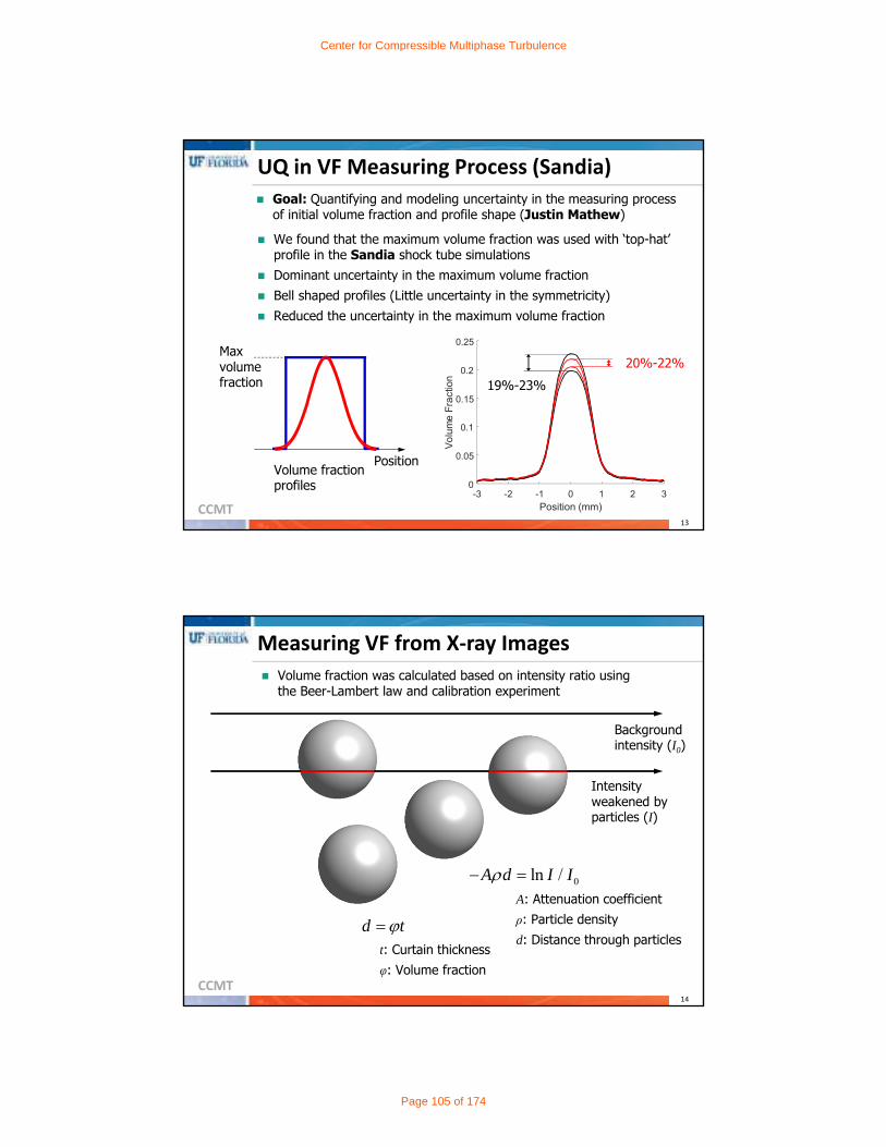
CCMT13

We found that the maximum volume fraction was used with ‘top-hat’ profile in the Sandia shock tube simulations

Dominant uncertainty in the maximum volume fraction Bell shaped profiles (Little uncertainty in the symmetricity) Reduced the uncertainty in the maximum volume fraction

-3 -2 -1 0 1 2 3Position (mm)

0

0.05

0.1

0.15

0.2

0.25

Vo

lum

eF

ract

ion

UQ in VF Measuring Process (Sandia)

Goal: Quantifying and modeling uncertainty in the measuring process of initial volume fraction and profile shape (Justin Mathew)

19%-23%20%-22%

Max volume fraction

PositionVolume fraction profiles

CCMT14

Volume fraction was calculated based on intensity ratio using the Beer-Lambert law and calibration experiment

Background intensity (I0)

Intensity weakened by particles (I)

0ln /A d I I A: Attenuation coefficientρ: Particle densityd: Distance through particles

d tt: Curtain thicknessφ: Volume fraction

Measuring VF from X‐ray Images


Page 105 of 174

CCMT15

00

ln //

I IA I I

d

Goals: Estimating the true trend and quantifying the uncertainty in the prediction

A constant attenuation coefficient does not fit the measured data well due to beam hardening

Calibration of A for Measuring VF

Wagner et. al (2015)

CCMT16

Calibrated A for Measuring VF

Assumed correlated noise in the data Made prediction of A and its uncertainty using

a Gaussian process model Considered linear and quadratic polynomial models (model form uncertainty) Obtained random attenuation curves based on the correlated noise model with

Monte Carlo simulations

0.6 0.7 0.8 0.9 1

I/I0

0.12

0.13

0.14

0.15

0.16

0.17

0.18

0.6 0.7 0.8 0.9 1

I/I0

0.13

0.14

0.15

0.16

0.17

0.18

0.19

Data95% CITrend pred.Random Trend

Data95% CITrend pred.Random Trend


Page 106 of 174

CCMT17

Uncertainty in Initial Volume Fraction

Two models gave similar results: little model form uncertainty The uncertainty in the attenuation coefficient was propagated mostly in

the uncertainty of the maximum volume fraction The uncertainty in the volume fraction profile was modeled with radial

basis function networks (RBFN)

Variability in VFLinear model

-1.5 -1 -0.5 0 0.5 1 1.50

0.05

0.1

0.15

0.2

0.25RBFN Regression

Position (mm)

Implementing the bell shaped profile for simulations

CCMT18

Summary of Sandia Mesoscale Campaign

1D Exp. w/ gap

Sampling U (Sim)Measurement U in PM (Exp)Sampling U (Exp)Measurement U in VF (Exp)U due to gap

1D Exp. w/o gap

Sampling U (Sim)Measurement U in PM (Exp)Sampling U (Exp)Measurement U in VF (Exp)

(80mm DFP from experiment)

0%

8%

16%

24%

Mod

eler

ror

estim

ate

( %)

Y1Q4 Y4Q1

Sandia campaign has been almost completed Found and reduced 1) the hidden error due to the use of AUSM+ and

2) the uncertainty due to the gaps Uncertainty in the initial volume fraction is the currently largest

uncertainty source in the model error estimate (down stream position)

Implementing the bell shaped profile for simulations


Page 107 of 174

CCMT

Macroscale

Mesoscale

Microscale


T5


Detonation

T5

T6T6












T4

T6T2

T6T4




T2

CCMT20

Shock tube overview: Four 32cm length segments Particle diameter: 45-90 microns Pressure ratio: ~20 Initial bed height: 32 cm

Goals: Plan new validation experiments that consider simulation

limitations and uncertainty quantification goals (Justin Mathew)

Identify sources of experimental uncertainty, quantifythose suspected to have a greatest influence on simulation inputs(Justin Mathew, Kyle Hughes)

UQ is involved in the experiment

UQ Involvement in ASU Experiment

4

3

2

Diaphragm


Page 108 of 174

CCMT21

Parameter Quantity Method

Diaphragm burst time ? Pressure sensor

Volume of particle bed 383.5-385.6 cm3

Initial volume fraction 59-65% CT scanner

Initial mean volume fraction 60-61% ∗ (Justin)

Particle diameter (before) 67±8 μm SEM

Particle diameter (after) 68±22 μm SEM

Particle density 2.44±0.006 g/cm3 Pycnometer

Driver section pressure 100.68±? kPa

Driven section pressure 5.5±? kPa

Tube geometry Negligible

Uncertain Experimental Parameters

Justin Mathew and Kyle Hughes actively involved in measuring the uncertainties

CCMT22

Particle Characterization – Shape/Size

Glass particles: 45-90 microns in diameter, 2.44±0.006 g/cm3

(Kyle Hughes and Justin at UF) Scanning electron microscope (SEM) Images show largely

homogenous groups of particles with no apparent source of significant variation (Kyle)

Scanning SEM images of particles after the experiment


Page 109 of 174

CCMT23

Particle Bed Characterization – Initial VF To verify estimates of ~61% average volume fraction measured during

ASU experiments, a mock particle bed was created for a CT scan The mock tube was only 7 mm in diameter

(versus ~40 mm shock tube diameter) Observed a mysterious volume fraction increase in the radial

direction

CCMT24

Preliminary Comparison and UQ There is inconsistency in measuring the bed heights The height data from the experiments is based on high speed camera

image while the simulation predicts height data based on volume fraction prediction

The uncertainty in t=0 has to be quantified accurately

Exp.5:

19

Exp.6:

20

ExperimentsSimulations


Page 110 of 174

CCMT25

New Experiment Planning

New experiments are conducted considering simulation limitations and UQ goals Usage of smaller particle sizes (45-90 micron)

to speed up simulation time Pressure probes distributed to reduce

uncertainty in diaphragm burst timing 1-3-2-2 distribution of pressure probes The lesson learned from UQ of the Eglin

microscale experiment Additional 2-3 cm of bed height added above

the clamp for better optical range

A

B

C

D D

A

B

C

CCMT

Macroscale

Mesoscale

Microscale



T4

T6SNL Mesoscale

Simulations



T2

T6T4







Detonation

T6T6






T5T5


Page 111 of 174

CCMT27


Schematic top-view of the test set-up.

Pressure probes

66”centerlin

e / shot line

NOT TO SCALE

D(θ)=34”

x

witness panel

Explosive Casing

Ph

anto

m

M31

0

Ph

anto

m

6.11

flash bulb

Xenon flash lamp

SIM

AC

ON

Near FieldFar Field

Source: Black, Littrell, and Delcambre, internal written

report, 3/7/2015

With a small number of particles, surprising evidence that the flow is strongly coupled with particles: Mean shock arrival times increase as the number

of particles is increased A possible explanation is high volume fraction in the

initial plane of the particles:

CCMT28

UF Analysis of Particles Used in Eglin

Eglin mesoscale gas gun experiment CT scans of particle packet, SEM of particles,

particle density via pycnometer Simacon and X-ray images to track particle

cloud movementsCT scans of particle packet for the Eglin mesoscale gas gun experiment

SEM of several steel particles at 500x zoom.

Eglin macroscale blastpad experiment SEM of particles and particle density via pycnometer Steel mock CT scan Comp B X-rays

75-125 µm Steel

Steel mock CT scan


Page 112 of 174

CCMT29

Casing fracture may be a possible mechanism for jetting instability

No significant effect from analytical estimation Steps taken to reduce the influence of the casing:

Thin phenolic tubing (3/16”) for the casing Failure energy ~0.06% of explosive energy

No casing between the explosive and particles Casing notched on outer surface to control case failure

Shot Liner Notched?1 ‐ ‐

2 ‐ ‐3 Tungsten Y4 Steel Y5 Steel Y

6 Steel N

Cross-section of the charge (side view) showing no inner casing

Cross-section of the charge (axial view) showing alignment of the notches with the pad surface

Side view of the tungsten (left) and steel (right) casing with notches

Controlling Casing Influence

CCMT30

Quantification of Numerical Error

Achieving convergence by modeling finite size particles


Page 113 of 174

CCMT

Macroscale

Mesoscale

Microscale


Quantification of Numerical Error

T4


T2

T6T4





Detonation




T5T5



T6SNL Mesoscale

Simulations


T6T6Eglin Microscale

Simulations


CCMT32

Summary and Overview

Goal: To achieve force convergence in a two-way coupled point particle Euler-Lagrange simulation using the finite size of the particles and to estimate the numerical error in the point-particle force (Samaun Nili)

In the point particle method, the particle feels the shock only if the shock reaches to the cell where particle center is located

When the particle diameter is larger than the grid size, the particle force shows an unrealistic jump at the center

The peak force increases as we reduce the grid size

dx

cell center

j j+1particle

Particle centershock

/ /

Point P

article


Page 114 of 174

CCMT33

The inhomogeneous flow felt by the particle represented by average over the surface or volume of the particle (Faxen theorem)

Computing the average volume and surface gas quantities and forces The numerical solution compared against the analytical solution

Proposed SolutionF

inite Size P

oint P

article

/ /

CCMT34

QS Force with Single Particle (115μm)

Point particle Finite size particle

0 0.5 1 1.5 2

time (t* = t/(DP/US))

0

50

100

150

200

f q s(k

N/k

g)

dx = 50 μm

dx = 12.5 μm

dx = 3.125 μm

Analytical

0 0.5 1 1.5 2

time (t* = t/(DP/US))

0

50

100

150

200

f qs(k

N/ k

g )

dx = 50 μm

dx = 12.5 μm

dx = 3.125 μmAnalytical


Page 115 of 174

CCMT35

Quasi‐Steady Force Convergence

RMSE measures the difference between analytical solution and finite size point particle model

RMSE decreases exponentially

1 10 40

Dp

/dx

10 0

10 1

RM

SE

(kN

/kg

)

Point Particle

Finite Size Point Particle

50 µm

25 µm

12.5 µm

6.25 µm3.125 µm100 µm

Particle (115μm)

Convergence direction

CCMT

Preparation for UQ of Macroscale Simulation

With Multi-Fidelity Surrogate


Page 116 of 174

CCMT

Macroscale

Mesoscale

Microscale


Preparation for UQ of Macroscale Simulation

T4

T6SNL Mesoscale

Simulations



T2

T6T4





Detonation

T6T6






T5T5



CCMT38

Multi‐Fidelity Surrogate for UQ

UQ often computationally expensive since it requires numerous simulation runs

Surrogates often provide good approximations based on several dozens of samples but even sampling for building a surrogate is not affordable for expensive simulations

Multi-fidelity surrogate: Approximating an expensive high fidelity simulation behavior by combining a few expensive high fidelity samples with cheap low fidelity samples

Low fidelity model selection: There are multiple lower fidelity models and selection is another questions to be answered

This technique is used for the collaboration with the exascale teamto approximate the CMT-bone with CMT-bone-BE and BE emulation


Page 117 of 174

CCMT39

Introduction to Multi‐Fidelity Surrogate

Goal: Approximating the high fidelity response based on a few high fidelity samples with low fidelity samples

0 0.2 0.4 0.6 0.8 1

x

-10

-5

0

5

10

15

20

ˆˆ ˆH Ly y x x x

ˆHy x

ˆLy x

x

: High fidelity simulation prediction: Low fidelity simulation prediction: Discrepancy prediction 0 0.2 0.4 0.6 0.8 1

x

-10

-5

0

5

10

15

0 0.2 0.4 0.6 0.8 1x

-10

-5

0

5

10

15

20

yL(x)=0.5y

H(x)+10(x-0.5)

yH

(x)=(6x-2)2sin(12x-4)

yL

yH

High fidelity function prediction

Discrepancy Prediction

CCMT40

MFS for UQ of 3D Sandia Shocktube Sim.

Goal: Approximating the 3D simulation for predicting front positions using 1D and/or 2D simulations

The simulations have the same grid resolution

Simulation parameters: Volume fraction Curtain thickness Mach number Random initial particle position

15 (3D) / 135 (2D) / 625 (1D) Computational cost ratios:

A single 3D run is equal to 25000 1D runs or 100 2D runs

A single 2D run is equal to 250 1D runs1.4 1.6 1.8

2

3

14

15

16

17

18

Thickness (mm)

Mach Number

Vol

ume

Fra

ctio

n (%

)

1D2D3D


Page 118 of 174

CCMT41

MFS Accuracies with 1D+3D and 2D+3D

Predicting downstream front position at 700 μs Using 11 other 3D runs to evaluate accuracy in terms of relative RMSE

(RMSE/max value) 0.025 (1D+3D) and 0.0875 (1D only) 0.0125 (2D+3D) and 0.0375 (2D only) 0.0638 (3D only)

DOE: 1D (125) +3D (4) DOE: 2D (27) +3D (4)

1.4 1.6 1.82

3

14

15

16

17

18

Thickness (mm)Mach Number

Vol

ume

Fra

ctio

n (%

)

1.4 1.6 1.82

314

15

16

17

18


Vol

ume

Fra

ctio

n (%

)

CCMT42

Difference Between 1D/2D/3D

MFS prediction allows to predict difference between models of different fidelities

For the shock tube simulation, the difference is most sensitive to Mach number

The difference between 3D and 1D is higher than that between 3D and 2D

Relative error in 2DRelative error in 1D

1.41.6

1.82

314

16

18


Vol

ume

Fra

ctio

n (%

)

-0.2

-0.15

-0.1

-0.05

0

0.05

0.1

1.41.6

1.82

314

16

18


Vol

ume

Fra

ctio

n (%

)

-0.08

-0.06

-0.04

-0.02

0

0.02

0.04

0.06

0.08


Page 119 of 174

CCMT43

Summary

Involvement of physics and UQ for experimental data extraction through measurement processing The initial volume fraction of the Sandia shock tube experiment

extracted from X-ray images using a X-ray attenuation model Rigorous UQ has reduced the initial uncertainty by 50%

Involvement of UQ team in measurement processing UQ of the ASU and Eglin experiments Planning those experiments for reducing measurement uncertainty

Quantifying numerical error in the particle force model by modeling finite size particles

Carrying out a study on Multi-fidelity surrogate for UQ and parametric study of hero simulations and BE emulation development

CCMT

CCMT



Page 120 of 174

CCMT45

3D dx=dy=dz=125μm

Legnth x Width x Height = 0.35 0.04 0.01 (M=1.45, 1.24)

Legnth x Width x Height = 0.38 0.04 0.01 (M=1.92)

6 million particles

Quartz 2048 cores wall time 24 hrs (max), 23 hrs+-20 mins

2D dx=dy=dz=125μm

Legnth x Width x Height = 0.35 0.04 125μm (M=1.45, 1.24)

Legnth x Width x Height = 0.38 0.04 125μm (M=1.92)

600,000 particles

Vulcan 128 cores wall time 40 hrs

1D dx=125μm

Legnth = 0.35 (M=1.45, 1.24)

Legnth = 0.38 (M=1.92)

5000 particles

Hipergator 4 cores wall time 20-30 mins

Computation Cost

CCMT46

1D/2D/3D Front Position Comparisons

Comparing 1D/2D/3D for two extreme combinations in terms of prediction metric (mean front positions)

M=1.24, 14%, 1.5 mm and M=192, 18%, 3.5 mm Variability due to initial particle positions is small for 1D

and negligible for 2D

0 2 4 6

Time (sec) 10-4

0

0.02

0.04

0.06

0.08

0.1

0 2 4 6

Time (sec) 10-4

0

0.005

0.01

0.015 Mean front positions(M=124, 14%, 1.5 mm)

1D2D3D

1D2D3D

Mean front positions(M=192, 18%, 3.5 mm)

1.4 1.6 1.82

3

14

15

16

17

18

Thickness (mm)

Mach Number

Vol

ume

Fra

ctio

n (%

)


Page 121 of 174

CCMT47

Slices from CT scan vs Rocpack

Mock Bed - CT Rocpack - CT

CCMT48

PVF Calculated Along Circular Region

Region PVF

Red 0.566

Blue 0.544

Yellow 0.568

Green 0.557

Cyan 0.562

Magenta 0.540

Nominal PVF = 0.54


Page 122 of 174

CCMT

CCMT

CMT-nek: CS Update

Sanjay RankaComputer and Information Science and Engineering

University of Florida

[email protected]

352 514 4213

CCMT2

Members

Tania Banerjee

KekeZhai

Mohamed Gadou

Sanjay Ranka

AdeeshaMalavi

Sai ChennaAravindNeelakantan


Page 123 of 174

CCMT3

Key Accomplishments (past year)

Dynamic load balancing of CMT-nek

Hybrid Multicore Computing using DVFS

Multi-level Memories and performance impact

CCMT4

Exascale Simulation: CS Challenges

Dynamic Load Balancing

B

A

Feasible space

Energy

Time

Energy and Performance

Tradeoffs

Future Architectures and Hybrid Processors

Parallelization on a million+ processors


Page 124 of 174

CCMT5

Talk Overview

CMT-bone/CMT-nek Dynamic Load Balancing

Colocation of particles with spectral elements

Mapping/Remapping Hybrid Multicore Processor

Hybrid Core Mapping KNL (Multi-level Memories) Power/Energy Modeling Dynamic Voltage Scaling Traditional Core (Autotuning) GPU (Manual Tuning)

Conclusions

CCMT6

CMT‐bone

Each cube represents a spectral element –formulation of the finite element method that uses high degree piecewise polynomials as basis functions

CMT-bone -- A Proxy Application for Compressible Multiphase Turbulent Flows, Jason Hackl, Mrugesh Sringarpure, Tania Banerjee, Tanzima Islam, S. Balachandar,Thomas Jackson, Sanjay Ranka, HiPC 2016, December 2016.


Page 125 of 174

CCMT7

Performance per Watt Improvement

Multi-LevelMemories

Power/Energy PerformanceTrade offs

Hybrid CoreMapping

Dynamic VoltageScaling

DynamicLoadBalancing

Auto Tuning

CMT-nekCMT-bone

Au

ton

tuin

g

Hyb

rid C

ore

Map

pin

g

Mu

lti Level M

emo

ries

Dyn

amic V

oltag

e Scalin

g

Dyn

amic L

oad

Balan

cing

X

Perfo

rman

ce E

nerg

y Tradeo

ffs

CCMT8

Dynamic Load Balancing: Expansion Fan


Page 126 of 174

CCMT9

Hero Run 2

CCMT10

Dynamic Load Balancing

Initialization Elements to processor mapping

Repeat the following steps Decide when to trigger a remap

Rebalance after every k time steps Rebalance when processing time per step gets higher beyond a

threshold If remap trigger = yes

Derive new elements to processor mapping Transfer elements and particles and reset other data structures

Serialize Communication Deserialize

Final Steps


Page 127 of 174

CCMT11

Serialization using Spectral Bisection

P1 – 8 particles P2 – 11 particles P3 – 8 particles

P4 – 5 particles

10

4 25 12 14

1 3 24 11 13

9 19

2

23 20

6 22 16 18

5 7 21 15 17

P4 – 8 particles

8

CCMT12

Elements to Processor Mapping


P4 – 5 particles P4 – 8 particles

(a) Default elements to processor mapping, agnostic of particles


Page 128 of 174

CCMT13

Elements to Processor Mapping


P4 – 8 particles P4 – 8 particles

(b) Elements to processor mapping, after taking into account both elements and particles

CCMT14

The Centralized Algorithm

Initially, each processor has an element load array

P0

3 6 4 5

P1

8 8 10 8

P2

7 3 7 3

Element load = # particles+ fluid load


Page 129 of 174

CCMT15


Each processor sends element load array to P0

P0

3 6 4 5

P1

8 8 10 8

P2

7 3 7 3

8 8 10 8 7 3 7 3

CCMT16


P0 receives and concatenates the element load array, computes the prefix sum, divides prefix sum by average load

3 9 13 18 26 34 44 52 59 62 69 72

0 0 0 0 0 1 1 2 2 2 2 2

3 6 4 5 8 8 10 8 7 3 7 3

P0 P1 P2

Prefix sum

Partition 1 Partition 2 Partition 3


Page 130 of 174

CCMT17


P0 distributes the assignment to other processors, and each processor gets the new elements

P0

3 6 4 5 8

P1

8 10

P2

8 7 3 7 3

CCMT18

The Distributed Algorithm

Each processor computes local prefix sum and the exclusive prefix sum of the element load on each processor

P0

P1 P2

3 9 13 18

8 16 26 34 7 10 17 20

18 34 20 0 18 52Exclusive prefix sum

Prefix sum


Page 131 of 174

CCMT19


Each processor adds the exclusive prefix sum to local prefix sum array to get the global prefix sum of element load array

8 16 26 34 7 10 17 20

3 9 13 18

26 34 44 52 59 62 69 72

0 18 52

0

3 9 13 18

18 52

P0

P1 P2

CCMT20


Each processor divides the global prefix array with the average load (in this case 24)

26 34 44 52 59 62 69 72

0 0 0 0

1 1 1 2 2 2 2 2

3 9 13 18

P0

P1 P2

24

24 24

Processor number


Page 132 of 174

CCMT21


Each processor keeps the elements that belong to them, and sends the remaining elements to the target processor

P0

3 6 4 5

P1

8 8 10

P2

8 7 3 7 3

Dynamic Load Balancing for Compressible Multiphase Turbulence, Keke Zhai, Tania Banerjee, David Zwick, Jason Hackl and Sanjay Ranka, submitted to IPDPS 2018

CCMT22

Rebalancing Time: Total Overhead (Quartz)

Overhead is about 220 and 121 time steps upon using centralized and distributed algorithms respectively

When extrapolated to a million ranks, centralized algorithm will take about 2300 time steps, whereas distributed algorithm will take 1800 time steps

y = 1E‐09x2 + 5E‐05x + 0.1215R² = 0.9397

y = 2E‐10x2 + 1E‐04x ‐ 0.0364R² = 0.9922

02468

101214

0 20000 40000 60000 80000

Tim

e (s

econ

ds)

MPI ranksCentralized DistributedPoly. (Centralized) Poly. (Distributed)

CMT-nek

Max: 73,728 MPI ranks4 elements / rank

343 particles / elementGrid size: 5x5x5Rarefaction test


Page 133 of 174

CCMT23

Expansion testcase: CMT‐nek on Quartz

Total time taken by CMT-nek is 4.62 hours Total time taken by load balanced code is 33 minutes Time per time step: 3.33 s for the original versus 0.4 s

for the load balanced code (balancing done every 300 s) Adaptive load balancing takes about 31 minutes total and

0.37 seconds per time step

CMT-nek67,206 MPI ranks

1,867 nodes36 cores per node900,000 elements 1.125x109 particles

Grid size: 5x5x5Rarefaction test

8.3x improvement in performance

0.000.501.001.502.002.503.003.504.00

0 1000 2000 3000 4000 5000

Tim

e pe

r Tim

e St

ep

(sec

onds

)

Simulation Time Steps (steps)

LoadBalanced Original

CCMT24

Power consumption is comparable

Expansion testcase: Power consumption on Quartz (using Libmsr)

0

20

40

60

80

100

Package Power Memory power

Pow

er (

Wat

ts)

Power components

Original Load Balanced


1,867 nodes36 cores per node900,000 elements 1.125x109 particles




Page 134 of 174

CCMT25

Rebalancing Time: Total Overhead Time (Vulcan)

When extrapolated to a million ranks, centralized algorithm will take 5.68s, whereas distributed algorithm will take 2.66s

Overhead is approximately is 9 time steps with centralized and 7 with distributed when 393,216 cores are used

y = 5E‐06x + 0.6782R² = 0.9996

y = ‐3E‐12x2 + 5E‐06x + 0.658R² = 0.9997

0

0.5

1

1.5

2

2.5

3

0 100000 200000 300000 400000 500000

Time (seconds)

MPI ranks

Centralized DistributedLinear (Centralized) Poly. (Distributed)

CMT-nekMax: 393,216 processors

2 elements / rank343 particles / element


CCMT26


8192 nodes4 cores per node460,800 elements

756,000,000 particlesGrid size: 5x5x5Rarefaction test


Expansion testcase: CMT‐nek on Vulcan

The original CMT-nek finished 800 steps in 5 hours Total time taken by load balanced code is 4.57 hours Time per time step: 21.2 seconds for the original versus

3.3 for the load balanced code

0.00

5.00

10.00

15.00

20.00

25.00

0 1000 2000 3000 4000 5000Tim

e pe

r Tim

e St

ep (

seco

nds)

Simulation Time Step (steps)

loadBalanced Original


Page 135 of 174

CCMT27

CMT-nek4,608 processors73,728 elements

86,400,000 particlesGrid size: 5x5x5Rarefaction test

0100200300400500600700800900

1000

Chipcore

DRAM Network SRAM Optics PCIExpress

LinkChipCore

Pow

er (W

atts

)

Power Domains

Original Load balanced

Core power and DRAM power reduced by about 5% and 2% respectively, leading to an overall reduction of 3.5% of total power when load balancing is used

Energy consumption of the load balanced code is better because of reduced time as well as reduced power consumption

Expansion testcase: Power consumption on Mira (Using MonEQ)

CCMT28

Hybrid Multicore ArchitecturesMulti-objective Load decomposition

Multi-objective Optimization on Hybrid Systems using DVFS, Mohamed Gadou, Sankeerth Mogili, Tania Banerjee, Sanjay Ranka, submitted to IPDPS 2018


Page 136 of 174

CCMT29

Theoretical formulation

E : Energy consumedn : Number of CPUsm : Number of GPUsf : CPU Frequencyg : GPU FrequencyS : Problem sizeT : Computation TimeT1 : Constrained timeO: Communication

overheadN : Total available CPUsM : Total available GPUsF : Set of available

CPU frequenciesG : Set of available

GPU frequencies

Minimize E(n, m, f, g, S)Subject to T(n, m, f, g, S) <= T1 – O(n, m, f, g, S)

n <= Nm <= Mf ∈ Fg ∈ G

248

127

16128 S

n CPU cores, freq f m GPU cores, freq gX S-X

Minimize ECPU(n, f, X) + EGPU(m, g, S-X)Subject to TCPU(n, f, X) <= T1 – Co(m+n, S)

TGPU(m, g, S-X) <= T1 – Co’(m, S-X)

n <= Nm <= Mf ∈ Fg ∈ G

248

127

344STCPU(n, f, X) × PCPU(n, f, X) TGPU(m, g, S-X) × PGPU(m, g, S-X)

TCPU(n, X)/f × PCPU(n, f) TGPU(m, S-X) /g × PGPU(m, g)344+32S

CCMT30

CPU Experiments

Parameters Valuesx, problem size in terms of number of elements (57)

1024, 1152, 1280, 1408, 1536, 1664, 1792, 1920, 2048, 2176, 2304, 2432, 2560, 2688, 2816, 2944, 3072, 3200, 3328, 3456, 3584, 3712, 3840, 3968, 4096, 4224, 4352, 4480, 4608, 4736, 4864, 4992, 5120, 5248, 5376, 5504, 5632, 5760, 5888, 6016, 6144, 6272, 6400, 6528, 6656, 6784, 6912, 7040, 7168, 7296, 7424, 7552, 7680, 7808, 7936, 8064, 8192

f, frequency in MHz (5) 1200, 1500, 1800, 2100, 2400

n, number of cores (5) 1, 2, 4, 8, 12


Page 137 of 174

CCMT31

CPU Experiments

02468

1012141618

1 2 4 8 12

Tim

e (s

econ

ds)

CPU cores

12001500180021002400

Frequency

Time per time step for processing a problem size of 8192 spectral elements and 256,000 particles

Experiments show time decreases by increasing CPU counts and frequency

CMT-bone8,192 elements

256,000 particlesGrid size: 7x7x7

CCMT32

CPU Experiments

0

0.1

0.2

0.3

0.4

0.5

0.6

2 4 8 12

Tim

e (s

econ

ds)

CPU cores

12001500180021002400

Frequency

CPU communication time for processing 8192 spectral elements and 256,000 particles

Communication time first decreases and then increases as processors are increased because volume of data communicated per core decreases in the beginning but the total communication volume begins to increase later




Page 138 of 174

CCMT33

Assumptions

Performance using lower clock frequencies may be derived from that using the highest clock frequency , , , ,

Power consumption does not depend on problem size , , ,

n = CPU count, f = CPU frequency, x = problem size

Example: Power lookup table:

f n 1 2 4 8 12

1200 93.24 97.33 101.32 114.46 127.501500 96.67 100.78 108.32 122.95 136.791800 98.14 102.88 111.53 131.86 148.452100 100.69 106.31 117.11 138.72 160.842400 102.65 108.12 123.94 145.54 167.08

CMT-bone

CCMT34

Prediction Error

Prediction error is within 3% for 99% of the tests

Performance


Power


Page 139 of 174

CCMT35

GPU Experiments

Parameters Valuesy, problem size in terms of number of elements (57)

Same problem sizes as described for CPUs.

g, frequency in MHz (3) 875, 810, 745

m, number of GPUs (4) 1, 2, 4, 8

CCMT36

GPU Experiments

00.20.40.60.8

11.21.41.6

1 2 4 8

Tim

e (s

econ

ds)

GPUs

745810875

Frequency

Time per time step for processing a problem size of 8192 spectral elements and 256,000 particles

Experiments show time decreases by increasing CPU counts and frequency




Page 140 of 174

CCMT37

GPU Experiments

0

0.1

0.2

0.3

0.4

0.5

0.6

1 2 4 8

Tim

e (s

econ

ds)

GPUs

745810875

Frequency

Total communication time when GPUs are used to solve the problem



CCMT38

Assumptions

Performance using lower clock frequencies may be derived from that using the highest clock frequency , , , ,

Power consumption does not depend on problem size , , ,

m = GPU count, g = GPU frequency, y = problem size

Example: Power lookup table:

g m 1 2 4 8745 89.79 169.91 314.53 550.91810 93.51 176.05 324.59 567.11875 98.80 185.46 341.26 589.41

CMT-bone


Page 141 of 174

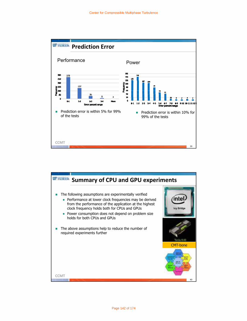
CCMT39

Prediction Error


Performance


Power

CCMT40

Summary of CPU and GPU experiments

The following assumptions are experimentally verified Performance at lower clock frequencies may be derived

from the performance of the application at the highest clock frequency holds both for CPUs and GPUs

Power consumption does not depend on problem size holds for both CPUs and GPUs

The above assumptions help to reduce the number of required experiments further

CMT-boneCMT-bone


Page 142 of 174

CCMT41

Hybrid Experiments

Parameters Values

Load (x, y)x = CPU loady = GPU load

(1024, 7168), (1152, 7040), (1280, 6912), (1408, 6784), (1536, 6656), (1664, 6528), (1792, 6400), (1920, 6272), (2048, 6144), (2176, 6016), (2304, 5888), (2432, 5760), (2560, 5632), (2688, 5504), (2816, 5376), (2944, 5248), (3072, 5120), (3200, 4992), (3328, 4864), (3456, 4736), (3584, 4608), (3712, 4480)

f 1200, 1500, 1800, 2100, 2400g 745, 810, 875n 2, 4, 8, 12m 1, 2, 4, 8

CCMT42

Hybrid Experiments

CPU GPU Predicted Energy (J)

Actual Energy (J)

Error%

elements count GHz elements count MHz

2540 8 2.4 5652 2 875 225.25 232.87 3.272621 8 2.4 5571 2 810 226.05 235.01 3.812621 8 2.4 5571 2 875 227.13 237.77 4.482540 8 2.4 5652 2 810 228.61 227.14 0.652293 8 2.4 5899 2 875 229.86 227.72 0.941474 4 2.4 6718 2 875 230.35 236.19 2.47

Error in prediction for some of the best predicted configurations for minimum energy consumption


Page 143 of 174

CCMT43

Hybrid Experiments

Energy versus performance pareto optimal curve. Red line shows the predicted curve, while blue line is obtained from actual data

Actual dataPredicted data

CMT-bone

CCMT44

5075

100125150175200225250275

0.3 0.35 0.4 0.45 0.5 0.55 0.6 0.65 0.7 0.75

Ener

gy (J

oule

s)

Time Per Time Step (Seconds)

Estimated Energy

Actual Energy

0.17, 8, 4, 2.4, 875, 243.95, 0.482 0.18, 8, 4, 2.4, 875,

241.35, 0.487

0.32, 8, 2, 2.4, 875, 227.10, 0.666

0.32, 8, 2, 2.4, 810, 226.05, 0.669

0.31, 8, 2, 2.4, 875, 225.25, 0.679

Pareto Curves for Energy Versus Runtime

Data for each Pareto-optimal point contain the following information in order:CPU load (%), CPU count, GPU count, CPU frequency (GHz), GPU frequency (MHz), energy (J), time (s)

0.26, 8, 2, 2.4, 810, 224.70, 0.666

0.15, 8, 4, 2.4, 810, 247.10, 0.5

0.28, 8, 2, 2.4, 875, 227.70, 0.657

0.15, 8, 4, 2.4, 875, 252.25, 0.498

0.31, 8, 2, 2.4, 745,223.40, 0.699


Page 144 of 174

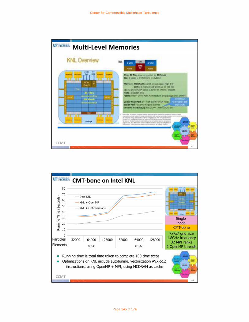
CCMT45

Multi‐Level Memories

CCMT46

CMT‐bone on Intel KNL

Running time is total time taken to complete 100 time steps Optimizations on KNL include autotuning, vectorization AVX-512

instructions, using OpenMP + MPI, using MCDRAM as cache

0

10

20

30

40

50

60

70

80

32000 64000 128000 32000 64000 128000

4096 8192

Runn

ing

Tim

e (S

econ

ds) Intel KNL

KNL + OpenMP

KNL + Optimizations

ParticlesElements

CMT-bone

Single node

7x7x7 grid size1.8GHz frequency

32 MPI ranks2 OpenMP threads


Page 145 of 174

CCMT47

CMT‐bone on Different Platforms

KNL is faster than an Intel IvyBridge by about 4 times KNL is faster than Tesla K40m GPU by about 3 times KNL is the most energy efficient platform

0

20

40

60

80

100

120

140

160

180

200

32000 64000 128000 32000 64000 128000

4096 8192

Runn

ing

Tim

e (S

econ

ds)

Intel Xeon

KNL + Optimizations

Tesla K40m

ParticlesElements

TDP: 150W

TDP: 245W

TDP: 215W

CCMT48

Publications1. Tania Banerjee and Sanjay Ranka, Genetic Algorithm based Autotuning Approach for

Performance and Energy Optimization, Proceedings of International Green and Sustainable Computing, 2015

2. Tania Banerjee, Mohammed Gadou, Sanjay Ranka, A Genetic Algorithm based Approach for Multi-objective Hardware/Software Co-optimization, Journal of Sustainable Computing, Vol 10, June 2016, 36 – 47.

3. Tania Banerjee, Jacob Rabb and Sanjay Ranka, Multi-objective Optimization of Spectral Solvers on Hybrid Multicore Platforms, Journal of Sustainable Computing, Vol 12, Dec 2016, 10 - 20.

4. Tania Banerjee, Jason Hackl, Mrugesh Sringarpure, Tanzima Islam, S. Balachandar, Thomas Jackson, Sanjay Ranka, CMT-bone -- A Proxy Application for Compressible Multiphase Turbulent Flows, Proceedings of HiPC, 2016

5. Mohamed Gadou, Tania Banerjee, Sanjay Ranka, Multi-objective Optimization of CMT-bone on Hybrid Processors, Proceedings of IGSC 2016

6. Tania Banerjee, Jason Hackl, Mrugesh Sringarpure, Tanzima Islam, S. Balachandar, Thomas Jackson, Sanjay Ranka, A New Proxy Application for Compressible Multiphase Turbulent Flows. Sustainable Computing: Informatics and Systems, 2017

7. Mohamed Gadou, Tania Banerjee, Meena Arunachalam, Sanjay Ranka, Multiobjectiveevaluation and optimization of CMT-bone on multiple CPU/GPU systems, Journal of Sustainable Computing: Informatics and Systems, 2017

8. Keke Zhai, Tania Banerjee, David Zwick, Jason Hackl and Sanjay Ranka, Dynamic Load Balancing for Compressible Multiphase Turbulence, submitted to IPDPS 2018

9. Mohamed Gadou, Sankeerth Mogili, Tania Banerjee, Sanjay Ranka, Multi-objective Optimization on Hybrid Systems using DVFS, submitted to IPDPS 2018

10.Mohamed Gadou, Meena Arunachalam, Tania Banerjee, Sanjay Ranka, Multiobjectiveevaluation and optimization of CMT-bone on Intel Knights Landing, in preparation.


Page 146 of 174

CCMT49

Conclusions: Overall Improvement

Au

ton

tuin

g

Hyb

rid C

ore

Map

pin

g

Mu

lti Level M

emo

ries

Dyn

amic V

oltag

e Scalin

g

Dyn

amic L

oad

Balan

cing

X

Perfo

rman

ce E

nerg

y Tradeo

ffs

020406080

100120140160180200

3200

0

6400

0

1280

00

3200

0

6400

0

1280

00Particles

Elements

TDP: 150W

TDP: 245W

TDP: 215W

Xeon

K40

KNL

Y

4096 8192

Algorithmic Hardware

Overall Improvement X*Y

Perform

ance per Watt Im

provement

CCMT

CCMT



Page 147 of 174

CCMT51

CPU Experiments

Constant of proportionality, for total execution time

Constant of proportionality, for communication time

f n 1 2 4 8 121200 0.975 0.965 0.965 0.935 0.905

1500 0.985 0.985 0.975 0.955 0.915

1800 0.995 0.995 0.990 0.985 0.975

2100 0.990 0.990 0.990 0.990 0.970

f n 1 2 4 8 121200 0.82 0.88 0.82 0.72 0.621500 0.86 0.86 0.86 0.77 0.701800 0.90 0.90 0.90 0.83 0.802100 0.95 0.95 0.95 0.92 0.90

CCMT52

Hardware‐Software Autotuning

Algorithm: dudr-4loopdo k = 1, Nz

do j = 1, Ny

do i = 1, Nx

do l = 1, Nx

dudr(I, j, k) = dudr(I, j, k) + a(i, l) * u(l, j, k, ie)

enddoenddo

enddoenddo

Algorithm: dudr-4loop-fuseddo k = 1, Nz* Ny

do i = 1, Nx

do l = 1, Nx

dudr(I, k) = dudr(I, k) + a(i, l) * u(l, k, ie)

enddoenddo

enddo

Algorithm: dudr-4loop-permuted-and unrolleddo k = 1, Nz

do i = 1, Nx

do j = 1, Ny

do l = 1, Nx,,2dudr(I, j, k) = dudr(I, j, k) +

a(i, l) * u(l, j, k, ie)dudr(I+1, j, k) = dudr(I+1, j, k) +

a(i, l+1) * u(l+1, j, k, ie)enddo

enddoenddoenddo

Number of 4-loop implementations for dudr Nx=Ny=Nz=10= 4! * 4 ^ 4= 24 * 256 = 6144 variantsTotal number of variants = 98,240 (N=10)Total number of variants = 217,728 (N=20)Exhaustive search may not be feasible

Total number of variants = 20


Page 148 of 174

CCMT53

Genetic Algorithm

i=1

• Compile and run each individual

• Set fitness value for each individual based on performance and energy

i < n ? Report the best individual

YesNo

• Population Selection

• Add new individuals using crossover and mutation

• i=i+1

• Generate Initial Population• i=1

CCMTY1‐ 54

Comparison of GA with Exhaustive Approach

Platforms CMT-nek time (seconds)

Exhaustive Autotuning

GA based Autotuning

Time

SearchSpace

%Less

Time SearchSpace

%Less

%Diff

IBM BG/Q 5.57 2.54 97716

54.3 2.58 1124 53.7 1.1

AMD Opteron

1.81 1.02 97716

43.6 1.06 1283 41.4 3.9

AMD Fusion 1.36 0.95 32652

30 0.95 485 30 0.0

Platforms

CMT-nekenergy (Joules)

Exhaustive Autotuning

GA based Autotuning

Energy

SearchSpace

%less

Energy

SearchSpace

%Less %Diff

IBM BG/Q

292.1 131.7 97716

54.9 135 1124 53.7 2.5

AMD Fusion

17.6 11.98 32652

32 12.11 485 31 1.1

Comparison of performance by platform

Comparison of energy consumption by platform

Results (AMD Fusion @ Sandia)


Page 149 of 174

CCMT55

Performance (varying hardware parameters)

Cache size

Line Size -Associativity

Best Time (seconds)

Power for most configurations is nearly the same. Thus, energy requirements are similar.

GEM5 environmentInstruction set architecture: X86CPU model: Out-of-order CPUMemory model: Classic, DDR3Clock frequency: 1GHz

Capacity Tuning

Associativity Tuning

Line Size Tuning

Genetic Algorithm based Autotuning Approach for Performance and Energy Optimization, Tania Banerjee and Sanjay Ranka (SUSCOM, to appear)


Page 150 of 174

CCMT

CCMT

ExascaleBehavioral Emulation

Principal Investigators:

Herman Lam, Greg StittCenter for Compressible Multiphase Turbulence (CCMT)

NSF Center for High‐Performance Reconfigurable Computing (CHREC)ECE Department, University of Florida

CCMT

Exascale Behavioral Emulation (BE) Team

| 2

Carlo PascoeFPGA Acceleration

Sai ChennaBE Design Space Exp.

Aravind NeelakantanBE Methods

Trokon JohnsonBE Tools

Chad SaundersFPGA Acceleration

Ryan BlanchardFPGA Acceleration

Raj RajagoplanBE-SST

Ben ReynoldsThermal Modeling

Nalini KumarBE Methods


Page 151 of 174

CCMT

Outline

Review & overview: – Behavioral Emulation (BE)

| 3

Researchthrusts&achievements– BE‐SST simulator & tools, experimental results

– BE method enhancements– Multi‐fidelity surrogate model for performance prediction

– Symbolic regression for performance modeling

– Thermal experiments & modeling

– CMT‐nek design space exploration using BE simulation

– Acceleration using FPGAs– Of BE: speedup vs BE‐SST, scale up on multiple FPGAs

– Of CMT‐nek kernels: approach & preliminary results

Summary, conclusions, & future work

CCMT

Outline

Review & overview: – Behavioral Emulation (BE)

| 4










Page 152 of 174

CCMT

Simulation Platforms

- BE SST

- FPGA Acceleration

BE

Sim

ula

tion

HW/SW co-design• Algorithmic & architectural design-space exploration (DSE)

Coarse-grained BE simulation• Balance of simulation speed & accuracy for rapid design-space evaluation

Co‐Design Using Behavioral Emulation

| 5

UQ team

* BEO – Behavioral Emulation Object

UQ team

Coarse-grainedSimulation Platforms

CMT-nekteam

CS team

CS team

CMT-nekteam

CCMT

Outline

Review & Overview: – Behavioral Emulation (BE)

| 6


– BE method enhancements– Multi‐fidelity surrogate model for performance prediction– Symbolic regression for performance modeling



– Acceleration using FPGAs– Of BE: speedup vs BE‐SST, scale up on multiple FPGAs– Of CMT‐nek kernels: approach & preliminary results



Page 153 of 174

CCMT

BE‐SST Simulator*

Developed by extending Structural Simulation Toolkit (SST)**– Framework for parallel simulations

– Supported by developers & vendors

– Flexibility in designing custom components

| 7

** From Sandia National Labs

* A. Ramaswamy, N. Kumar, H. Lam, and G. Stitt, “Scalable Behavioral Emulation of Extreme-Scale Systems Using Structural Simulation Toolkit”, submitted to the International Parallel and Distributed Processing Symposium (IPDPS), Vancouver, CA., May 21-25, 2018.

CCMT

BE‐SST Enhancements

Developed interpolation API– To select appropriate interpolation techniques (e.g., Linear

interpolation, polynomial interpolation)

Since AST review 2017: support for symbolic regression– Improve accuracy (More details later)

Able to support trace‐driven simulation* – For time‐dependent simulations

– To mimic CMT‐nek with particles more accurately

Inclusion of collective‐communication operations– MPI_ISEND, MPI_IRECV, MPI_WAITALL

Communication model– Replaced static routing method with dynamic routing

Leverage parallel capabilities of SST for BE‐SST

| 8* More details in Sai Chenna’s presentation on Tuesday


Page 154 of 174

CCMT

Dynamic Routing

| 9

Replaced static routing method with dynamic routing– Improve BE‐SST scaling: large static routing table not required for

increasing number of cores (Fig. 1)

– Build‐time benefits: Config build time not a bottleneck for large simulation (Fig. 2)

Fig. 1 Static vs. Dynamic Routing Fig. 2 BE‐SST parallelized on 64 cores on HiPerGator @UF

CCMT

Parallel Performance of BE‐SST

| 10

Simulations of Vulcan System

with 5‐D Torus Topology*

– 4K, 32K, 128K core

Improved parallel performance

with increase in problem size

– For e.g., 128k core simulation

• Without parallelization (1 rank): ~1 day;

• With 256‐rank parallelization: 17 min.

* Run using BE-SST installed on Titan


Page 155 of 174

CCMT

BE‐SST Scalability

Aiming for 1M+ cores; able to simulate 800K+ – Memory bottleneck

Uneven memory distribution across ranks while simulating– Bigger systems (e.g., 1 Million+ cores)

– With more complex interconnects (e.g., 5D Torus of Vulcan)

| 11

* GCM Graph Construction Memory: initial memory allocation before simulation

Working with Sandia National Labs (Jeremy Wilke) to solve this issue

*

CCMT

Outline


| 12








Page 156 of 174

CCMT

BE simulations of HPC systems

Titan @ ORNL– Cray XK7 architecture with Cray Gemini interconnect– 16‐core AMD opterons; 18k nodes; 300k cores– 18k K20X Kepler GPUs– 32GB + 6GB memory/node

| 13

Vulcan @ LLNL– IBM BG/Q architecture– 16 cores/node, 24k nodes, 390k cores– 16GB memory/node

CCMT

Application Case Study: CMT‐bone‐BE

CMT‐nek & CMT‐bone (mini‐app) both are large codes

To support extensive DSE*, we need:– Key compute kernels & comm. patterns that affect performance

– Abstract, modular, easy to modify and instrument for algorithmic DSE

| 14

CMT‐nek Workflow (highlighted portions represented in CMT‐bone‐BE) Computation‐ & communication‐

intensive portions of CMT‐nekworkflow in C & MPI– Volume‐to‐surface data extraction– Face data exchange (with neighbors)– Derivative computation volume points

Easier to modify for algorithmic DSE

1000 vs 10s of thousands lines of code

* design-space exploration


Page 157 of 174

CCMT

Experiment Setup

Application case study: CMT‐bone‐BE (gas solver)

Application parameters– Calibration

• element size: 5,9,13,17,21• elements/core: 8,32,64,128,256

– Validation • element size: 5,6,9,11,16,17• 64 elements/core

Machine parameters– Validation up to 128k MPI ranks

– Predictions up to 1M MPI ranks

– Can perform both predictions and validations for larger systems

Monte‐Carlo Simulations

| 15

CCMT

0.199 0.201 0.203 0.2050.00

00.

003

0.0

06

Execution Time (seconds)

De

nsity

0.1925 0.1930 0.1935 0.1940 0.19450.0

000

.004

0.0

08

Execution Time (seconds)

Den

sity

BE Simulations of CMT‐bone‐BE on Titan+

Simulating bigger system than Titan (up to 1 Million cores)

Average % error between CMT‐bone‐BE simulation and execution time is 4%

Maximum error is 17%

| 16

BE Simulation

CMT-bone-BE Execution

%

∑ ∑

∑ 100

100 runs & 100 simulations


Page 158 of 174

CCMT

0321k32k1Me-3

e-2

e-1

0e+

1e+

2e+

3

4 6

810

1214

1618

MPI ranks (no. of processor cores)

avg

. exe

cutio

n ti

me

/tim

est

ep

(s)

BE simulation TestbedMeasured

BE Simulations of CMT‐bone‐BE on Vulcan+

Simulating a bigger system than Vulcan (512k cores)

Average % error between CMT‐bone‐BE simulation and execution time is 4%

Maximum error is 9%

| 17

BE Simulation

CMT-bone-BE Execution

100 runs & 100 simulations

CCMT

BE Simulations of CMT‐bone‐BE on Notional Architecture

Notional architecture– IBM POWER architecture– 48 cores/node– Non‐blocking fat‐tree topology– Tending towards Summit @ ORNL

Initial methodology– OSU n/w benchmark* of Cab (fat‐tree topology)

– Lookup tables of Vulcan (POWER architecture)

– Predictions up to 128k MPI ranks

| 18*developed in Ohio State University Work in progress


Page 159 of 174

CCMT

Outline


| 19







CCMT

Behavioral Emulation with UQ

Goal: Improve BE models via validation and uncertainty estimation

– Reduce computational budget by fitting BE simulation to CMT‐nek using Multi‐Fidelity Surrogate (MFS)

– Extrapolation of CMT‐nek towards large‐scale runs using BE and MFS

| 20

w/ UB


Page 160 of 174

CCMT21

Element SizeNumber of processors

Ele

men

ts p

er p

roce

ssor

Multi‐fidelity Prediction of CMT‐nekExperimental setup

Design of experiment (DOE)– Element size (ES) = 5,9,13,17,21– Elements per processor (EPP) = 8,32,64,128,256– Number of processors (NP) = 16,256,2048,16384,131072

125 total data points

* BE simulation: all 125 runs

CMT‐nek: 22 runs

CMT‐bone: 67 runs

Multi‐fidelity surrogate model– Fitting CMT‐nek using corrected fitting of BE simulation– For large problems, low‐fidelity BE simulation is computationally

cheaper than high‐fidelity CMT‐nek or CMT‐bone

w/ UB

CCMT22

Accuracy of corrected BE sim. At 10 left‐out CMT‐nek test points

Overall RMSE < 10% with 7 or more CMT‐nek data

Reducing computation budget

– Supplementing high‐fid. (CMT‐nek) with low‐fid. (BE simulation) runs

w/ UB

2 4 6 8 10 12

Number of CMT-nek data

10 0

10 1

10 2

10 3

RM

SE

of

pe

rce

nt

err

or(

%)

Corrected BE simulation against CMT-nek

Corrected BE simulation

BE simulation

Initial RMSE comparison: – BE‐simulation vs CMT‐nek at all experimental points

– Overall root mean squared error (RMSE) 74%

(Initial RMSE comparison)

Multi‐fidelity Prediction of CMT‐nek

Y. Zhang, A. Neelakantan, N. Kumar, C. Park, R. Haftka, N. H. Kim, and H. Lam, “Multi-fidelity Surrogate Modeling for Application/Architecture Co-design”, accepted to Performance Modeling, Benchmarking and Simulation of High Performance Computer Systems (PMBS17), Denver, CO, Nov. 13, 2017.


Page 161 of 174

CCMT23

Extrapolation Towards Large‐scale Runs

Extrapolation necessary for exascale prediction – But challenging due to limited runs

Develop MFS using:– 7 (out of 22) runs of CMT‐nek (high‐fidelity), at 256 and 2k processors– All 125 BE simulations (low‐fidelity)

Extrapolate using MFS towards 16k (11 runs) & 128k (4 runs) processors

w/ UB

* 125 BE simulation22 CMT-nek runs

CCMT24

Extrapolation: Validation

Extrapolate using MFS towards 16k (11 runs) and 128k (4 runs) processors – Linear fit to CMT‐nek: poor result

High‐order fitting leads to overfitting due to limited samples (7 CMT‐nek runs with 3 variables)

– MFS: relative errors less than 11%

w/ UB


Page 162 of 174

CCMT25

Extrapolation: Prediction of CMT‐nek

MFS prediction towards one million processors with UQ– 64 elements per processors (9 CMT‐nek runs )

– MFS predictions )

Monotonic trend with small curvature in logarithmic coordinate

w/ UB

CCMT

Outline


| 26

Researchthrusts&achievements

– BE‐SST simulator & tools, experimental results







Page 163 of 174

CCMT

Symbolic Regression: Motivation

Motivation:

– Multi‐parameter performance modeling is challenging

– Requires accuracy, computational efficiency, simple implementation

Our previous approaches:

– N‐dimensional interpolation:• Computationally expensive

• Difficult to implement, needs customization for each example

• Insufficient accuracy

– Multi‐variate linear regression:• Faster than interpolation, relatively simple to implement

• Need thorough understanding of code to generate performance models

• May not capture machine‐specific behaviors that deviate from basic model

| 27

CCMT

Symbolic Regression

| 28

Linear Regression for O(x2) Symbolic Regression

Advantages:

– Captures machine‐specific performance behaviors

– Enables tradeoffs between accuracy and computational complexity

• Can maximize performance for a given error constraint

– Requires no prior knowledge of the kernel

Approach: custom genetic‐programming tool

– Evolves “trees” from mathematical primitives

– Multiple optimization goals: minimize error, minimize error given tree size constraint, minimize tree size given error constraint, etc.


Page 164 of 174

CCMT

Symbolic Regression: Results

| 29

Particle solver kernelLinear Regression Symbolic Regression Error Improvement

MAPELinear/MAPEsymbolicRMSE MAPE RMSE MAPE

Compute1 4.43E-06 3.5% 1.08E-05 1.5% 2.4x

update_particle_location 1.26E-05 10.8% 1.26E-05 1.6% 6.8x

particles_in_nid 1.17E-02 76.4% 1.27E-02 31.1% 2.5x

interp_props_part_location 4.51E-01 902.6% 3.67E-01 10.0% 90.7x

upd_vel_and_pos_rk3_stage1 8.22E-04 399.0% 5.43E-04 9.0% 44.2x

upd_vel_and_pos_rk3_stage3 1.06E-04 19.4% 6.50E-05 9.7% 2.0x

upd_vel_and_pos_rk3_allstage 7.34E-03 27.3% 7.57E-04 6.8% 4.0x

upd_vel_and_pos_bdf 5.38E-04 20.0% 1.21E-03 4.9% 4.1x

red_interp 9.33E-02 4.7% 2.94E-02 4.3% 1.1x

usr_particles_forces 8.80E-05 6.3% 6.85E-05 2.1% 2.9x

tri_interp 1.58E-04 1.4% 5.34E-05 0.7% 1.9x

Average 5.14E-02 133.8% 3.75E-02 7.4% 14.8x

CCMT

Outline


| 30

Researchthrusts&achievements

– BE‐SST simulator & tools, experimental results







Page 165 of 174

CCMT

Thermal Benchmarking & Modeling Previously modeled energy/power using physical and simulation

measurements

Current focus: thermal modeling with IR images of KNL

– Goal: minimize maximum temperature via load balancing

More challenging than anticipated

– CPU fans block thermal information of CPU

– Tried custom fan setup, destroyed several processors

Modified KNL for IR by cutting hole in case:

| 31

CCMT

Thermal Benchmarking & Modeling

Observations:

– Heat sink “blocks” much of processor

– Minimizing the maximum temperature may not be most appropriate optimization goal

Future work: investigate how heat changes for different load balancing optimizations

– Determine most approach optimization goal

| 32

Nek-5000 on KNL (64 cores) Nek-5000 on KNL (1 core) hot

cold


Page 166 of 174

CCMT

Outline


| 33







CCMT34

CMT‐nek DSE: Motivation & Approach

Motivation:

– CMT‐nek has huge design space

– Various architectural options exist for Exascale systems

Goal:

– Use BE methods & tools to perform DSE

– Approach: Iterative DSE steps

• Perform BE Simulations of CMT‐nek(baseline)

• Identify optimization candidates (i.e. most expensive subroutines )

• Create and validate models of algorithms for these subroutines

• Use BE to predict performance


Page 167 of 174

CCMT35

BE‐SST Predictions: Particle solver

Summary of results

– Interpolation:• scales non‐linearly w.r.t element size and elements‐per‐

processor, linearly w.r.t particles/gridpoint

• Reduced barycentric is 5x faster than barycentric interpolation

• Trilinear interpolation is on average 164x faster than barycentric interpolation

– Time integration:• scales non‐linearly w.r.t element size and elements‐per‐

processor, linearly w.r.t particles/gridpoint

• Bdf is 3x faster than rk3 time integration

Refer to Sai Chenna’s presentation

– BE Simulations of CMT‐nek

CCMT

Outline


| 36










Page 168 of 174

CCMT

BE Design‐Space Exploration

BE Advantage: significantly faster than existing simulators

BE Limitation: still not fast enough for DSE of exascale systems

Approach: Use FPGA acceleration to improve exploration

– Sacrifice analysis capabilities to prune design space

– Use BE‐SST to analyze remaining candidates

| 37

BE Simulator (SW) ~Minutes per simulation

Optimized Design

Example design space:• 20 values for lelt, lx1, lpart• 10 different numbers of cores• 10 different core types• 10 different memory configurations• 4 different network topologies

32 million options to explore

CCMT

Fully‐expanded Pipeline (FEP)

1. Construct Data Flow Graph (DFG) from simulation configuration– AppBEO+ArchBEO define instructions

and operand/output dependencies – Instructions map to vertices and

dependencies map to edges in DFG– Various opportunities for graph‐level

optimizations

| 38

prev.s

MM FUNC.

mm_out.s

prev.s1

RECV FUNC.

recv_out.s

prev.s

1. Extracting DFG from BE simulation configuration

2. Mapping DFG to FPGA Pipeline

send

mm

recv

recv

send

mm

DFG if(id==0) send;else recv;mm;if(id==0) recv;else send;

proc

proc

com

m ArchBEOS

AppBEOS

Configuration Mapping

Type: compSubtype: mmTID: 0EID: 1Parameters: [256,256,256]

Type: commSubtype: recvTID: 1EID: 0STID: 0SEID: 0, msgsize

…

Event AttributesPipelined Simulation

Because each instruction (from sim) mapped to independent HW (no resource sharing), each vertex able to start next sim 1 cycle after current sim

2. Map DFG to pipeline circuit– Vertex attributes define operations and

instantiate dedicated HW– Edge attributes (e.g., src/dst) instantiate

pipeline register between src/dst pair– Various opportunities for circuit‐level

optimizations


Page 169 of 174

CCMTBecause each subgraph instruction mapped to independent HW, each vertex able to start next subgraph 1 cycle after current subgraph. All subgraphs must complete before sim can complete

Collapsed Pipeline (CP)

1. Construct Data Flow Graph (DFG) from simulation configuration– AppBEO+ArchBEO define instructions

and operand/output dependencies – Instructions map to vertices and

dependencies map to edges in DFG– Partition into linear subgraphs and

generate dependency lists

| 39

1. Extracting DFG, then identify subgraphs & dependencies

2. Mapping DFG to FPGA Pipeline

send

mm

recv

recv

send

mm

DFG if(id==0) send;else recv;mm;if(id==0) recv;else send;

proc

proc

com

m ArchBEOS

AppBEOS

Configuration Mapping

2. Map DFG to pipeline circuit– Vertex attributes define operations and

Edge attributes instantiate pipeline register between src/dst pairs

– Align subgraph traces such that cost is minimized and no dependencies are violated

send

mm

recv

recv

send

mm

DFG

(1,1) (2,1)(2,3) (1,3)

send mm recv

Align delay delay

mm delayrecv send delay

recv

Map

send delay delay

delayrecv send delay

mm

mux

mux

CCMT

Fully‐Expanded & Collapsed Pipeline Tradeoffs

| 40

Fully-Expanded PipelineAdvantages:─ Superior performance in terms of simulation throughput and latency

─ 280 - 320 MHz implies 280 - 320 million simulations per second independent of simulated MPI ranksLimitations:─ Resources scale linearly with both MPI Ranks and number of timesteps─ Scaling across multiple FPGAs expected to be ineffective when considering exascale simulations

Ranks TSNum. ofEvents

% LULatency(cycles)

HardwareMSPS†

HardwareGEPS‡

BE-SSTKEPS‡

Hardware Speedup

32 1 1,344 15 / 2 64 / 278 300 / 10.5 403 / 14.1 4.4 92x106 / 3x106

32 2 2,688 31 / 3 118 / 512 300 / 10.5 806 / 28.2 7.8 103x106 / 4x106

32 3 4,032 46 / 4 172 / 746 300 / 10.5 1,210 / 42.3 10.6 114x106 / 4x106

32 4 5,376 61 / 6 226 / 980 300 / 10.5 1,613 / 56.4 12.9 125x106 / 4x106

32 5 6,720 76 / 7 280 / 1,214 300 / 10.5 2,016 / 70.6 14.8 136x106 / 5x106

32 6 8,064 92 / 9 334 / 1,488 300 / 10.5 2,419 / 84.7 16.5 147x106 / 5x106

32 8 10,752 – / 12 – / 1,916 – / 10.5 – / 113 19.1 – / 6x106

32 16 21,504 – / 24 – / 3,788 – / 10.5 – / 226 24.2 – / 9x106

32 32 43,008 – / 44 – / 7,532 – / 10.5 – / 452 28.9 – / 16x106

64 1 2,880 32 / 2 65 / 394 300 / 5.23 864 / 15.1 7.7 112x106 / 2x106

64 2 5,760 65 / 4 119 / 712 300 / 5.23 1,728 / 30.1 12.6 137x106 / 2x106

64 3 8,640 99 / 5 173 / 1,030 300 / 5.23 2,592 / 45.2 16.2 160x106 / 3x106

64 4 11,520 – / 7 – / 1,348 – / 5.23 – / 60.2 17.9 – / 3x106

64 8 23,040 – / 14 – / 2,620 – / 5.23 – / 121 23.2 – / 5x106

64 16 46,080 – / 29 – / 5,164 – / 5.23 – / 241 26.9 – / 9x106

64 32 92,160 – / 46 – / 10,252 – / 5.23 – / 482 29.1 – / 17x106

128 1 5,952 66 / 2 66 / 458 300 / 2.62 1,786 / 15.6 10.8 165x106 / 1x106

128 2 11,904 – / 4 – / 776 – / 2.62 – / 31.2 14.9 – / 2x106

128 3 17,856 – / 5 – / 1,094 – / 2.62 – / 46.8 17.1 – / 3x106

128 4 23,808 – / 7 – / 1,412 – / 2.62 – / 62.4 18.4 – / 3x106

128 8 47,616 – / 15 – / 2,684 – / 2.62 – / 125 20.8 – / 6x106

128 16 95,232 – / 30 – / 5,228 – / 2.62 – / 250 22.3 – / 11x106

128 32 190,464 – / 47 – / 10,316 – / 2.62 – / 499 22.8 – / 22x106

†Mega-Simulations-Per-Second, ‡Giga/Kila-Events-Per-Second, ‘–’ indicates configuration unable to fit on a single FPGA


Page 170 of 174

CCMT


% LULatency(cycles)

HardwareMSPS†

HardwareGEPS‡

BE-SSTKEPS‡

Hardware Speedup

32 1 1,344 15 / 2 64 / 278 300 / 10.5 403 / 14.1 4.4 92x106 / 3x106

32 2 2,688 31 / 3 118 / 512 300 / 10.5 806 / 28.2 7.8 103x106 / 4x106

32 3 4,032 46 / 4 172 / 746 300 / 10.5 1,210 / 42.3 10.6 114x106 / 4x106

32 4 5,376 61 / 6 226 / 980 300 / 10.5 1,613 / 56.4 12.9 125x106 / 4x106

32 5 6,720 76 / 7 280 / 1,214 300 / 10.5 2,016 / 70.6 14.8 136x106 / 5x106

32 6 8,064 92 / 9 334 / 1,488 300 / 10.5 2,419 / 84.7 16.5 147x106 / 5x106

32 8 10,752 – / 12 – / 1,916 – / 10.5 – / 113 19.1 – / 6x106

32 16 21,504 – / 24 – / 3,788 – / 10.5 – / 226 24.2 – / 9x106

32 32 43,008 – / 44 – / 7,532 – / 10.5 – / 452 28.9 – / 16x106

64 1 2,880 32 / 2 65 / 394 300 / 5.23 864 / 15.1 7.7 112x106 / 2x106

64 2 5,760 65 / 4 119 / 712 300 / 5.23 1,728 / 30.1 12.6 137x106 / 2x106

64 3 8,640 99 / 5 173 / 1,030 300 / 5.23 2,592 / 45.2 16.2 160x106 / 3x106

64 4 11,520 – / 7 – / 1,348 – / 5.23 – / 60.2 17.9 – / 3x106

64 8 23,040 – / 14 – / 2,620 – / 5.23 – / 121 23.2 – / 5x106

64 16 46,080 – / 29 – / 5,164 – / 5.23 – / 241 26.9 – / 9x106

64 32 92,160 – / 46 – / 10,252 – / 5.23 – / 482 29.1 – / 17x106

128 1 5,952 66 / 2 66 / 458 300 / 2.62 1,786 / 15.6 10.8 165x106 / 1x106

128 2 11,904 – / 4 – / 776 – / 2.62 – / 31.2 14.9 – / 2x106

128 3 17,856 – / 5 – / 1,094 – / 2.62 – / 46.8 17.1 – / 3x106

128 4 23,808 – / 7 – / 1,412 – / 2.62 – / 62.4 18.4 – / 3x106

128 8 47,616 – / 15 – / 2,684 – / 2.62 – / 125 20.8 – / 6x106

128 16 95,232 – / 30 – / 5,228 – / 2.62 – / 250 22.3 – / 11x106

128 32 190,464 – / 47 – / 10,316 – / 2.62 – / 499 22.8 – / 22x106

†Mega-Simulations-Per-Second, ‡Giga/Kila-Events-Per-Second, ‘–’ indicates configuration unable to fit on a single FPGA

Fully‐Expanded & Collapsed Pipeline Tradeoffs

| 41

Collapsed PipelineAdvantages:─ Resources scale linearly with timesteps, but sublinearly with MPI Ranks

─ allows for significantly more timesteps due to its much lower base utilization─ Better scaling on single and multiple FPGAsLimitations:─ Lower simulation throughput and longer initial latency, but still more than sufficient for rapid design-space exploration

CCMT

Collapsed Pipeline Single‐FPGA Performance/Scalability

| 42

As number of ranks increase:─ additional logic per rank approaches zero─ simulation throughput reduced by a factor of “ranks”─ event throughput remains proportional to instantiated event hardware

Pipelines scale linearly with length of simulation, however blockram eventually becomes limiting resource ─ e.g., only fit 2 TS for 1 million ranks on Stratix V─ Motivation to explore partially-collapsed pipeline approach

Increased performance expected with Stratix 10─ Collapsed hardware specifically designed to exploit

new Stratix 10 architecture


% LULatency(cycles)

HardwareMSPS†

HardwareGEPS‡

BE-SSTKEPS‡

Hardware Speedup

32 32 43,008 44 7,532 10.5 450 10.14 44x106

64 32 92,160 46 10,252 5.23 482 24.91 19x106

128 32 190,464 47 10,316 2.62 498 24.42 20x106

256 32 393,216 67 13,516 1.31 515 23.92 21x106

512 32 811,008 84 20,684 0.65 531 21.47 25x106

1K 32 1,646,592 84 21,196 0.33 539 18.21 29x106

32K 32 55,443,456 84 241,868 1.02x10‐2 567 12.96 44x106

128K 16 111,673,344 46 333,932 2.56x10‐3 285 8.91 32x106

1M 2 112,459,776 5 1,148,056 3.19x10‐4 36 X X

*Collapsed performance of CMT-Bone-BE with varied MPI ranks and simulation timesteps on a single Stratix V S5GSMD8K1F40C2 @ 335MHz

Now able to reach million+ rank simulations in hardware

Rank limit due to insufficient blockram not logic

Expect greater performance when Stratix 10 becomes available

Throughput > 10Mx higher than BE-SST


Page 171 of 174

CCMT

Collapsed Pipeline Multi‐FPGA Performance/Scalability

| 43

8 ProceVnodes

Novo‐G# 64 GiDEL ProceV (Stratix V) 4x4x2 3D torus or 5D hypercube 6 Rx‐Tx links per FPGA Measured 32 Gbps per link 150 ns latency across links

Ranks TS FPGAs Num. of EventsLat to First

Out (cycles)*Mega Sims

/second*Giga Events

/second*

1K 32 1 1,646,592 21,196 0.33 539

1K 64 2 3,293,184 41,439 0.33 1,077

1K 128 4 6,586,368 81,925 0.33 2,15532K 32 1 55,443,456 241,868 1.02E-2 567

32K 64 2 110,886,912 451,039 1.02E-2 1,134

32K 128 4 221,773,824 869,381 1.02E-2 2,267128K 32 2 223,346,688 536,863 2.56E-3 571128K 64 4 446,693,376 942,725 2.56E-3 1,142128K 128 8 893,386,752 1,754,449 2.56E-3 2,2831M 32 16 1,799,356,416 2,641,321 3.19E-4 5751M 64 32 3,598,712,832 4,234,137 3.19E-4 1,1501M 128 64 7,197,425,664 7,414,540 3.19E-4 2,299

Pipelines scale linearly with the length of simulation, but as a single, unidirectional pipe─ Partitioned easily/predictably across any number of connected FPGAs

Given a desired # of simulated ranks, timesteps, granularity (events per timestep), we can predict performance & # of FPGAs

Main point: FPGAs achieve similar scale as BE-SST, but orders of magnitude faster─ 1M ranks, 300+ of sims/second

*Predicted collapsed performance of CMT-Bone-BE with varied MPI ranks and simulation timesteps on multiple Stratix V S5GSMD8K1F40C2 @ 335MHz

Require 64bits/cycle between FPGAs 335MHz, 21.4 Gbps, 51 additional lat 450MHz, 28.8 Gbps, 68 additional lat 500 MHz before link BW saturation

C. Pascoe, S. Chenna, G. Stitt, H. Lam, “A FPGA-Pipelined Approach for Accelerated Discrete-Event Simulation of HPC Systems”, accepted to Heterogeneous High-performance Reconfigurable Computing (H2RC), Denver, CO, Nov. 13, 2017.

CCMT

Outline


| 44










Page 172 of 174

CCMT

FPGA Acceleration Trends

FPGAs growing trend in data centers– Microsoft Catapult, Amazon F1,

Intel Broadwell+FPGA

– National lab interest

Recently performed case study on Intel Broadwell+Arria 10 (BDW+A10) for 2D convolution– 96x less energy than Broadwell

– 15.7x less energy than P6000 GPU

Future research?– FPGA acceleration of CMK‐nek

functions

| 45

Energy Comparison of BDW+A10 vs. P6000 GPU

Energy Comparison of BDW+A10 vs. Broadwell

Precision Kernel Size 256x256 512x512 1024x1024 2048x2048 Avg

16‐bit Fixed 3x3 35× 47× 67× 68× 54×

5x5 68× 116× 171× 179× 133×

7x7 58× 135× 153× 164× 128×

9x9 44× 98× 135× 148× 106×

Avg 51× 99× 131× 140×

32‐bit Float 3x3 33× 46× 65× 66× 53×

5x5 64× 111× 162× 169× 127×

7x7 55× 113× 131× 139× 109×

9x9 32× 58× 71× 75× 59×

Avg 46× 82× 108× 112×

Image Size

Precision Kernel Size 256x256 512x512 1024x1024 2048x2048 Avg

16‐bit Fixed 3x3 15.5× 19.8× 19.4× 19.0× 18.4×

5x5 12.9× 18.6× 19.5× 19.8× 17.7×

7x7 10.5× 18.2× 19.7× 20.5× 17.2×

9x9 8.1× 15.3× 16.9× 18.6× 14.7×

Avg 11.8× 18.0× 18.9× 19.5×

32‐bit Float 3x3 14.6× 19.4× 19.0× 18.6× 17.9×

5x5 12.2× 17.8× 18.6× 18.7× 16.8×

7x7 9.9× 15.2× 16.9× 17.3× 14.8×

9x9 5.8× 9.0× 8.9× 9.4× 8.3×

Avg 10.6× 15.4× 15.8× 16.0×

Image Size

CCMT

Summary & Conclusions

BE methods & tools– BE method enhancements: network models, interpolation &

symbolic regression schemes, energy & thermal modeling– BE‐SST enhancements: functionality, tools, & scaling

Large‐scale experiments– Validation (100k+ MPI ranks) on Titan & Vulcan– Predictive simulations to million+ MPI ranks; on notional archs

CMT‐nek DSE using BE simulation– Profiling of key CMT‐nek particle solver routines– Accuracy/performance tradeoffs using BE simulation

FPGA acceleration of BE simulation– Validation of dataflow, pipelined approaches (FEP, CP) – multi‐FPGA scalability prediction & validation

| 46


Page 173 of 174

CCMT

CCMT



Page 174 of 174

tst review october 30‐31, 2017 · tst review october 30-31, 2017 attendee list faculty s....

Documents