ts ten con - old dominion universitytkennedy/cs350/sum15/public/reqts/...purp ose this sensor y arra...

Technical Report # TR{93{06

A Formal Speci�cation of the

RSDIMU Inertial Navigation System

Steven Zeil, Aileen Biser, Linghan Cai, Hong Huang,

Tijen Ireland, Brian Mitchell, and George Walker

Old Dominion University

Department of Computer Science

Norfolk, VA 23529-0162

U.S.A.

March 12, 1993

Updated: April 7, 1993

This work was supported by grant NAG-1-439 from the NASA Langley Research Center.

Abstract

This document presents a formal speci�cation for the Rsdimu, a component of an aircraft inertial

navigation system. The speci�cation is written in the Z language.

The Rsdimu system consists of a set of eight acceleration sensors, mounted upon the four upright

faces of a square based pyramid (i.e., a semi-octohedron), two sensors per face. The purpose of

this sensor array is to provide a measure of the current acceleration of the aircraft within which

it is mounted. The eight sensors provide redundancy during the estimate of the 3-dimensional

acceleration. This redundancy permits valid accleration estimates in the face of sensor failures and

aids in reducing error due to noise in the sensor readings.

Keywords: Formal Speci�cations, Z, Rsdimu

Contents

1 Introduction 2

1.1 The RSDIMU : : : : : : : : : : : : : : : : : : : : : : : : : : : : : : : : : : : : : : : : 2

1.2 History of This Speci�cation : : : : : : : : : : : : : : : : : : : : : : : : : : : : : : : : 3

1.3 Conventions : : : : : : : : : : : : : : : : : : : : : : : : : : : : : : : : : : : : : : : : : 3

2 Coordinate Systems 4

2.1 Basic De�nitions : : : : : : : : : : : : : : : : : : : : : : : : : : : : : : : : : : : : : : 4

2.2 Transformations : : : : : : : : : : : : : : : : : : : : : : : : : : : : : : : : : : : : : : 5

2.3 Special-Case Transformations : : : : : : : : : : : : : : : : : : : : : : : : : : : : : : : 7

2.3.1 Yaw, Pitch, and Roll : : : : : : : : : : : : : : : : : : : : : : : : : : : : : : : : 7

2.3.2 Misalignment : : : : : : : : : : : : : : : : : : : : : : : : : : : : : : : : : : : : 7

2.3.3 Pyramids : : : : : : : : : : : : : : : : : : : : : : : : : : : : : : : : : : : : : : 8

2.4 Pure Rotations : : : : : : : : : : : : : : : : : : : : : : : : : : : : : : : : : : : : : : : 10

3 Physical Structure 10

3.1 Sensors : : : : : : : : : : : : : : : : : : : : : : : : : : : : : : : : : : : : : : : : : : : 11

3.2 Faces : : : : : : : : : : : : : : : : : : : : : : : : : : : : : : : : : : : : : : : : : : : : : 12

3.3 The Instrument : : : : : : : : : : : : : : : : : : : : : : : : : : : : : : : : : : : : : : : 14

3.4 The RSDIMU State : : : : : : : : : : : : : : : : : : : : : : : : : : : : : : : : : : : : 15

4 Calibration and Failure Detection 17

4.1 Vehicle At Rest : : : : : : : : : : : : : : : : : : : : : : : : : : : : : : : : : : : : : : : 17

4.1.1 Calibration - Calculating Sensor O�sets : : : : : : : : : : : : : : : : : : : : : 17

4.1.2 Failures From Noisy Sensors : : : : : : : : : : : : : : : : : : : : : : : : : : : : 18

4.2 In-Flight Failure Detection : : : : : : : : : : : : : : : : : : : : : : : : : : : : : : : : 19

4.2.1 The Test Threshold : : : : : : : : : : : : : : : : : : : : : : : : : : : : : : : : 20

4.2.2 Edges : : : : : : : : : : : : : : : : : : : : : : : : : : : : : : : : : : : : : : : : 20

4.2.3 Checking The Edge-Vectors : : : : : : : : : : : : : : : : : : : : : : : : : : : : 21

4.2.4 Isolating Sensor Failure : : : : : : : : : : : : : : : : : : : : : : : : : : : : : : 22

4.2.5 Calibration and Failure Detection : : : : : : : : : : : : : : : : : : : : : : : : 24

5 Vehicle Acceleration Estimation 25

5.1 Overview : : : : : : : : : : : : : : : : : : : : : : : : : : : : : : : : : : : : : : : : : : 25

5.2 Channels : : : : : : : : : : : : : : : : : : : : : : : : : : : : : : : : : : : : : : : : : : 25

5.3 Basic Calculations : : : : : : : : : : : : : : : : : : : : : : : : : : : : : : : : : : : : : 26

5.4 Acceleration Estimation : : : : : : : : : : : : : : : : : : : : : : : : : : : : : : : : : : 29

6 The Display 31

6.1 The Display Panel : : : : : : : : : : : : : : : : : : : : : : : : : : : : : : : : : : : : : 31

6.2 The Display Interface : : : : : : : : : : : : : : : : : : : : : : : : : : : : : : : : : : : 35

7 Initialization 40

8 Conclusions 41

References 41

Index 43

1

A

B

C

D

Figure 1: The RSDIMU Instrument Package

1 Introduction

1.1 The RSDIMU

This document presents a formal speci�cation for the Rsdimu navigation sensor system. The speci-

�cation is written in the Z language.

The Rsdimu problem was previously isolated as a subject for studies in the e�ectiveness of

software redundancy for fault tolerance [3, 4]. A requirements document [1] was developed jointly

by sta� of the Research Triangle Institute and of Charles River Analytics.

The Rsdimu (Redundant Strapped-Down Inertial Measurement Unit) system consists of a set

of eight acceleration sensors, mounted upon the four upright faces of a square based pyramid (i.e.,

half of a regular octahedron), two sensors per face. Figures 1 and 2 illustrate this structure. The

purpose of this sensor array is to provide a measure of the current acceleration of the aircraft within

which it is mounted. The eight sensors provide redundancy during the estimate of the 3-dimensional

acceleration. This redundancy permits valid acceleration estimates in the face of sensor failures and

aids in reducing error due to noise in the sensor readings. The redundancy management software

for the Rsdimu is charged with the following tasks:

� Calibration of the accelerometers with the aircraft at rest (subject only to gravitational accel-

eration),

� Analysis of noise in the accelerometer readings,

� Detection of failed sensors based upon

{ excessive noise in readings from an individual sensor, or

{ inconsistency of an individual sensor's readings as compared to readings from the others,

� Estimation of the aircraft acceleration using those calibrated sensors deemed to be operational.

This speci�cation covers the description of the Rsdimu hardware interface, the pre- ight calibra-

tion, and a subsequent single (instantaneous) estimate of vehicle acceleration while in- ight. More

realistically, we would expect the Rsdimu to be included within a larger navigation system that

would perform a continuous series of such estimates, integrating them over time to determine the

2

60 60

x y

Figure 2: Sensor Mounting on RSDIMU Faces

position and velocity of the aircraft. In [1], however, the validation process calls for only a single

estimate.

1.2 History of This Speci�cation

The speci�cation presented in this document was developed by the instructor and students of the

Fall 1992 class in \Formal Methods in Software Engineering" at the Old Dominion University De-

partment of Computer Science. After approximately 7 weeks instruction in notations for writing

formal speci�cations, with emphasis on the Z language [2], the instructor (Steven Zeil) presented the

students with the general framework for the Z speci�cation. This framework corresponds roughly to

Sections 2 and 3 of the following document. Responsibility for the remainder of the requirements

speci�cation [1] was then distributed among the students. In particular, students were asked to

specify the process of calibration and sensor failure detection, the process of estimating vehicle ac-

celeration from the calibrated sensors, and the hardware/software subsystem for the Rsdimu display

panel. In the course of developing these speci�cations, the students suggested various changes to the

instructor's original speci�cation of the physical components of the sensor array (Section 3). The

resulting speci�cations have been collected by the instructor to form this document.

The organization of this document follows a roughly bottom-up presentation of the Rsdimu.

Section 2 presents the \background" mathematics upon which the Rsdimu is based | vectors and

transformations in 3-space. Section 3 presents the physical construction of the Rsdimu sensor array.

Section 4 describes the calibration and failure detection procedures. Section 5 describes the process

of estimating the current acceleration of the vehicle. Finally, Section 6 speci�es the Rsdimu output

display panel.

1.3 Conventions

Most of the notation used here is standard Z. This has been augmented in a few instances with

standard linear algebraic conventions (such as the ability to write vectors and matrices in the usual

rectangular forms).

In addition, certain lexical conventions are employed in selecting names. Names of individual

objects or variables begin with lower-case letters, although upper case letters are used within multi-

3

word names to indicate the start of each distinct word. Schema names and data type names each

begin with upper-case letters. The names of schemas that indicate state (rather than state transi-

tions) are generally singular noun phrases. Data type names, on the other hand, are plural noun

phrases. These two often occur in related pairs. For example, \Sensor" is the name of a schema

describing the state of an arbitrary linear acceleration sensor. \Sensors" is the name of the data

type comprised of all possible objects that satisfy the Sensor schema.

In the original requirements document [1], a number of names are given for objects that are

required to appear as types, variables, or constants in an acceptable implementation. To maintain a

clear link to that document, we have attempted to use those names whenever possible, even in cases

where we believe that clearer names would have contributed to easier understandability. For example,

the name linstd denotes the maximum acceptable value for the standard deviation of accelerometer

readings from any sensor. While the \std" part of the name clearly indicates standard deviation, and

the \lin" is a convention used consistently to indicate input from a linear accelerometer, nothing in

this name suggests that it represents a maximum threshold rather than an actual standard deviation

value for some sensor. We might have preferred a name max linstd or max operational lin std , but

have opted to keep the name \as is" to maintain compatibility with [1].

Some consistent changes are made to the names taken from [1]. The requirements document spells

out the need to maintain separate variables for many input and output quantities. For example, an

array of sensor failure information occurs in [1] as linfailin and linfailout . Because Z is quite adept

at distinguishing input and output quantities, we have consistently removed the \in" and \out"

designations from variable names, preferring instead to employ the Z decorations. For example, we

have linfail for the failure information prior to any state change, and linfail

0

for the updated failure

information after a state change.

2 Coordinate Systems

2.1 Basic De�nitions

This section sets up some basic concepts about coordinate systems and transformations of

point/vector coordinates from one system to another.

To begin with, de�ne 3-dimensional vectors and matrices, indexed by the typical direction names

x ; y ; z .

DirectionNames == fx ; y ; zg

Vectors3D == DirectionNames ! <

TransformMatrices == (DirectionNames � DirectionNames)! <

I will assume that the conventional linear algebraic operations have been de�ned on these types,

and that the conventional vector/matrix tabular forms are understood.

Some convenient constants are

identity : TransformMatrices

zero3D : Vectors3D

identity = f d : DirectionNames � (d ; d) 7! 1:0 g

[f d1; d2 : DirectionNames j d1 6= d2 � (d1; d2) 7! 0:0 g

zero3D = f d : DirectionNames � d 7! 0:0 g

or, alternatively

4

identity : TransformMatrices

zero3D : Vectors3D

identity =

2

4

1 0 0

0 1 0

0 0 1

3

5

zero3D =

2

4

0

0

0

3

5

In de�ning directions and points, we have two choices. Both are conventionally written as a

3-tuple of <, in other words, a Vectors3D . That, however, assumes that the coordinate system is

known from context. In this application, we are dealing with so many di�erent coordinate systems,

a simple vector of three numbers would be easily misinterpreted. So we will say that directions and

points must carry their appropriate coordinate system with them:

[Frames]

Point

coord : Vectors3D

x ; y ; z : <

system : Frames

x = coord(x )

y = coord(y)

z = coord(z )

As a convenience, the coordinates of a point p can be accessed individually (p:x ; p:y ; p:z ) or as an

entire coordinate vector (p:coord).

Direction

Point

p

coord(x )

2

+ coord(y)

2

+ coord(z )

2

= 1:0

We will want to use points and directions as types, so next we de�ne appropriate sets to serve as

types:

Points == fPointg

Directions == fDirectiong

2.2 Transformations

A Transformation describes how to move from one coordinate system (frame) to another:

Transformation

rotation : TransformMatrices

translation : Vectors3D

Transformations == fTransformationg

5

Using these, we can de�ne a function transforming vectors from one coordinate system to another:

transform : (Vectors3D � Transformations)! Vectors3D

transform = � v : Vectors3D ; t : Transformations �

t :rotation � (v + t :translation)

A frame identi�es a coordinate system. Most frames are de�ned relative to other frames. Trans-

formations are transitive. If we can transform from frame A to frame B , and can transform from

B to C , then we can also transform directly from A to C . Because of this, if we are describing a

world containing many frames, we need not give transformations between each pair of frames, but

only those frames that are most closely and simply related to one another.

A world, then is a collection of related frames:

Worlds : P(Frames � Frames) 7! Transformations

8w :Worlds; f : Frames �

w(f ; f ):rotation = identity ^ w(f ; f ):translation = zero3D

What if we want to transform coordinates between two frames not directly related within our

world? If we can �nd a chain of related frames, we can come up with the composite transformation

information:

translation between : (Frames � Frames �Worlds) 7! Vectors3D

translation between =

f f 1; f 2 : Frames; w :Worlds; t : Transformations j

(f 1; f 2) 7! t 2 w � (f 1; f 2;w) 7! t :translation g

[f f 1; f 2; f 3 : Frames; w :Worlds; t : Transformations j

(f 1; f 2) 7! t 2 w � (f 1; f 3;w) 7! t :translation + translation between(f 2; f 3;w) g

rotation between : (Frames � Frames �Worlds) 7! TransformMatrices

rotation between =

f f 1; f 2 : Frames; w :Worlds; t : TransformMatrices j

(f 1; f 2) 7! t 2 w � (f 1; f 2;w) 7! t :rotation g

[f f 1; f 2; f 3 : Frames; w :Worlds; t : TransformMatrices j

(f 1; f 2) 7! t 2 w � (f 1; f 3;w) 7! t :rotation � rotation between(f 2; f 3;w) g

Using these, we can de�ne a function transforming points from one coordinate system to another

within a world:

DoTransform

p? : Points

w? :Worlds

from?; to? : Frames

p! : Points

t : Transformations

t :rotation = rotation between(from?; to?;w?)

t :translation = translation between(from?; to?;w?)

p!:coord = transform(p?:coord ; t)

p!:system = to?

6

transform : (Points � Frames �Worlds) 7! Points

transform = f DoTransform � (p?; from?; to?;w?) 7! p! g

2.3 Special-Case Transformations

Transformations between frames may be computed in many ways. This section is devoted to various

special case approaches to obtaining transformations. In particular, we consider the designation of

a rotation by yaw, pitch and roll angles, the designation of a general rotation through very small

angles, and transformations among the planar faces of a semi-octahedron.

2.3.1 Yaw, Pitch, and Roll

If both frames are orthogonal, the rotation is often speci�ed by three angles called the \yaw", \pitch",

and \roll". The yaw angle, often denoted by , is a rotation about the z-axis and yields a transform

yaw : Angles ! TransformMatrices

yaw =

8

<

:

: Angles � 7!

2

4

cos sin 0

� sin cos 0

0 0 1

3

5

9

=

;

The pitch is a subsequent rotation about the resulting Y axis (after applying the yaw).

pitch : Angles ! TransformMatrices

pitch =

8

<

:

� : Angles � � 7!

2

4

cos � 0 � sin �

0 1 0

sin � 0 cos �

3

5

9

=

;

The roll is a subsequent rotation about the resulting X axis (after applying the yaw and pitch).

roll : Angles ! TransformMatrices

roll =

8

<

:

� : Angles � � 7!

2

4

1 0 0

0 cos� sin�

0 � sin� cos�

3

5

9

=

;

The composite transformation is then de�ned as

yaw pitch roll : (Angles � Angles � Angles)! TransformMatrices

yaw pitch roll( ; �; �) = yaw( ) � pitch(�)) � roll(�)

We can also de�ne its inverse:

roll pitch yaw : (Angles � Angles � Angles)! TransformMatrices

roll pitch yaw( ; �; �) = roll(��) � pitch(��) � yaw(� )

2.3.2 Misalignment

Misalignment describes a small rotation into a (usually) non-orthogonal coordinate system. For

each of the three axes in the \ideal" coordinate system, the corresponding axis in the misalignment

system is described by a pair of small rotations around the other two ideal axes. These rotations are

7

\small" in the sense that they are rotations through an angle � small enough that � and sin � are

approximately equal (when � is measured in radians).

Each misalignment angle is labeled with a pair of axes names.

MisalignmentNames == fxy ; xz ; yx ; yz ; zx ; zyg

MisalignmentAngles == MisalignmentNames ! Angles

The �rst name is the axis described by the misalignment angle. The second is the axis about which

the rotation occurs. For example, �

xy

describes the rotation of the x axis around the y axis.

The misalignment angles can be used to obtain a transform matrix as follows

toMisaligned :MisalignmentAngles ! TransformMatrices

toMisaligned =

8

<

:

� :MisalignmentAngles �

2

4

1 �(xz ) ��(xy)

��(yz ) 1 �(yx )

�(zy) ��(zx ) 1

3

5

9

=

;

The inverse is

fromMisaligned :MisalignmentAngles ! TransformMatrices

fromMisaligned =

8

<

:

� :MisalignmentAngles �

2

4

1 ��(xz ) �(xy)

�(yz ) 1 ��(yx )

��(zy) �(zx ) 1

3

5

9

=

;

2.3.3 Pyramids

The following de�nitions describe the transformation from a single frame I into a series of four frames

whose x � y planes form a semi-octahedron with its base centered on the origin of the I frame.

1

It's not exciting, but it is necessary.

De�ne the following family of vectors:

StoI : (FaceNames � DirectionNames) 7! Vectors3D

StoI =

8

<

:

(A; x ) 7!

1

2

p

3

2

4

p

3 + 1

�

p

3 + 1

�2

3

5

(A; y) 7!

1

2

p

3

2

4

�

p

3 + 1

p

3 + 1

�2

3

5

(A; z ) 7!

1

p

3

2

4

1

1

1

3

5

(B ; x ) 7!

1

2

p

3

2

4

�

p

3 + 1

�

p

3� 1

�2

3

5

(B ; y) 7!

1

2

p

3

2

4

p

3 + 1

p

3� 1

�2

3

5

(B ; z ) 7!

1

p

3

2

4

1

�1

1

3

5

(C ; x ) 7!

1

2

p

3

2

4

�

p

3� 1

p

3� 1

�2

3

5

(C ; y) 7!

1

2

p

3

2

4

p

3� 1

�

p

3� 1

�2

3

5

(C ; z ) 7!

1

p

3

2

4

�1

�1

1

3

5

(D ; x ) 7!

1

2

p

3

2

4

p

3� 1

p

3 + 1

�2

3

5

(D ; y) 7!

1

2

p

3

2

4

p

3� 1

�

p

3 + 1

�2

3

5

(D ; z ) 7!

1

p

3

2

4

�1

1

1

3

5

9

=

;

Then we can de�ne the following transformation matrices:

1

In Section 3, the frame I will be designated as the \Instrument" frame, and the other four frames as the faces A,

B, C , and D of the Rsdimu instrument package.

8

T

AI

;T

BI

;T

CI

;T

DI

;T

IA

;T

IB

;T

IC

;T

ID

: TransformMatrices

T

AI

=

2

4

StoI (A; x )

T

StoI (A; y)

T

StoI (A; z )

T

3

5

T

BI

=

2

4

StoI (B ; x )

T

StoI (B ; y)

T

StoI (B ; z )

T

3

5

T

CI

=

2

4

StoI (C ; x )

T

StoI (C ; y)

T

StoI (C ; z )

T

3

5

T

DI

=

2

4

StoI (D ; x )

T

StoI (D ; y)

T

StoI (D ; y)

T

3

5

T

IA

=

�

StoI (A; x ) StoI (A; y) StoI (A; z )

�

T

IB

=

�

StoI (B ; x ) StoI (B ; y) StoI (B ; z )

�

T

IC

=

�

StoI (C ; x ) StoI (C ; y) StoI (C ; z )

�

T

ID

=

�

StoI (D ; x ) StoI (D ; y) StoI (D ; z )

�

And, given, the following constant,

pyrO�set ==

1

p

6

2

4

0

0

�1

3

5

a series of transform functions can then be de�ned:

AtoI : < ! Transformations

8 r : < � (

AtoI (r):rotation = T

AI

^

AtoI (r):translation = r � pyrO�set)

BtoI : < ! Transformations

8 r : < � (

BtoI (r):rotation = T

BI

^

BtoI (r):translation = r � pyrO�set)

CtoI : < ! Transformations

8 r : < � (

CtoI (r):rotation = T

CI

^

CtoI (r):translation = r � pyrO�set)

DtoI : < ! Transformations

8 r : < � (

DtoI (r):rotation = T

DI

^

DtoI (r):translation = r � pyrO�set)

ItoA : < ! Transformations

8 r : < � (

ItoA(r):rotation = T

IA

^

ItoA(r):translation = �r � pyrO�set)

9

ItoB : < ! Transformations

8 r : < � (

ItoB(r):rotation = T

IB

^

ItoB(r):translation = �r � pyrO�set)

ItoC : < ! Transformations

8 r : < � (

ItoC (r):rotation = T

IC

^

ItoC (r):translation = �r � pyrO�set)

ItoD : < ! Transformations

8 r : < � (

ItoD(r):rotation = T

ID

^

ItoD(r):translation = �r � pyrO�set)

2.4 Pure Rotations

In many cases, we aren't really concerned with the translation portion of a transformation. It is there-

fore convenient to have a function for converting TransformMatrices directly into Transformations:

rotate : TransformMatrices ! Transformations

8M : TransformMatrices �

rotate(M ):rotation = M ^ rotate(M ):translation = zeros3D

3 Physical Structure

The RSDIMU is composed of an instrument and a display. The display is discussed in Section 6.

This section is devoted to the structure of the instrument package.

There are a number of frames associated with the RSDIMU problem. They are named as follows:

Frames == fnavigation; vehicle; instrument ;A;B ;C ;D ;

~

A;

~

B ;

~

C ;

~

Cg

The frames A : :D are collectively known as the sensor frames of reference, and the frames

~

A : :

~

D are

the measurement frames. The measurement frames are paired with the sensor frames in the obvious

manner:

measureFor == fA 7!

~

A;B 7!

~

B ;C 7!

~

C ;D 7!

~

Dg

The acceleration due to the earth's gravity, measured in the navigation frame, is de�ned as:

g

N

: Vectors3D

g

N

=

2

4

0

0

g

3

5

10

3.1 Sensors

Each face of the Rsdimu instrument package contains a pair of linear sensors, known as the x and

y sensor for that face (see Figure 2).

SensorNames : PDirectionNames

SensorNames = fx ; yg

Each sensor produces a 12-bit digital output indicating a voltage proportional to the acceleration

along the direction of the sensor. This 12 digit value is called a \count". The counts obtained from

the sensors are proportional to the acceleration (in

meters

sec

2

) along the direction of that sensor.

Counts == 0 : : 4096

Accelerations == <

Sensors are physical devices and produce noisy output. The largest standard deviation that would

be expected from a functional sensor is given as the value linstd :

linstd : Counts

Like most physical measurement devices, the sensors are sensitive to temperature changes:

Temperatures == <

Sensor

linFail : boolean

prevFailed : boolean

o�Raw : seqCounts

scale0; scale1; scale2 : <

temp : Temperatures

slope : <

speci�cForce : Accelerations

linO�set : Accelerations

linNoise : boolean

defective : boolean

rawl : Counts

lin : Accelerations

slope = scale0 + scale1 � temp + scale2 � temp

2

speci�cForce = linO�set + slope � (rawl � 2048)=409:6 (1)

lin = speci�cForce

standardDev(o�Raw) > 3 � linstd ) defective

prevFailed ) linFail

linNoise ) linfail (2)

linFail ) defective

For each sensor, linFail represents the known state of the sensor (true if the sensor is known to be

defective). Determining the proper value of this �eld is a major task of the calibration procedure

11

(Section 4). A sequence of values o�Raw are used for this purpose, and also help to compute the

proper linO�set used in converting the raw data into proper force measurements (the speci�cForce).

prevFailed is the state of the sensor prior to any calibration and estimation activities.

The temperature of the sensor is given by temp, and the scale factors scale0, scale1, and scale2

(determined at the factory) combine with temperature to determine the slope, which also is used to

determine the speci�cForce.

If the noise (standard deviation) in the measurements o�Raw exceeds 3 � linstd , then the sensor

will be marked as noisy (linNoise set to true) and therefore failed (linFail set to true) during the

calibration procedure. Here, we model this by introducing a variable defective indicating the \true"

state of the sensor. This variable will be hidden from the rest of the system.

Note that linFail ) defective, but not defective ) linFail , because a sensor may be defective

without our knowing it until the calibration procedure has been completed. Note also that this

simple check of the standard deviation is not the only way to determine that a sensor is defective.

Sensors may also be marked as defective during the \edge-vector test" portion of the calibration, in

which the consistency of sensors from adjacent faces is checked.

The current reading of the sensor is given as rawl . lin is the name given in the requirements for

the current speci�c force.

Finally, we turn the above schema into a data type, hiding the \true" status:

Sensors == f Sensor n defective g

3.2 Faces

The instrument package is a semi-octahedron (a square-based pyramid) (Figure 1). It has four

non-base faces, named by the sensor frame:

FaceNames : PFrames

FaceNames = fA;B ;C ;Dg

FaceStatus = fnonOperational ; partiallyOperational ; completelyOperationalg

12

GeneralFace

sensorFrame : FaceNames

measurementFrame : Frames

world :Worlds

sensors : Sensors ! Sensors

misalign :MisalignmentAngles

temp : Temperatures

normFace : Accelerations

status : FaceStatus

speci�cForceMF : Points

speci�cForceSF : Points

measuredAccel : SensorNames 7! Accelerations

measurementFrame = measureFor(sensorFrame)

8m :MisalignmentNames � misalign(m) � sinmisalign(m)

sensors(x ):temp = sensors(y):temp = temp

world = f

(sensorFrame;measurementFrame) 7! rotate(toMisaligned(misalign));

(measurementFrame; sensorFrame) 7! rotate(fromMisaligned(misalign))g

speci�cForceMF =

2

4

sensors(x ):speci�cForce

sensors(y):speci�cForce

normFace

3

5

speci�cForceSF = transform(speci�cForceMF ;measurementFrame; sensorFrame;world)

Each face is named either A, B , C , or D , i.e., faces are named for one of the sensor frames. There

is also a corresponding measurement frame representing the physical mounting of the sensors.

Each face contains two sensors, named the x and y sensors. There is an ideal position for each

sensor, but the physical mounting may di�er slightly. The di�erences are speci�ed as the misalign

angles for each sensor (see Section 2.3.2). The misalignment angles are assumed to be small enough

(less than 5 degrees) for the sine of the angle to be approximately equal to the value of the angle

expressed in radians.

The temperature of the face, temp, determines the temperatures of the sensors mounted on the

face.

During the calibration procedure, the face is subjected to a known acceleration normFace normal

(perpendicular) to the face.

The total speci�c force vector acting on this face, as measured by this face's sensors, is given

in the measurement and sensor frames by speci�cForceMF and speci�cForceSF , respectively. The

measuredAccel is the quantity used in the actual acceleration estimation procedure.

CompletelyOperationalFace

GeneralFace

status = completelyOperational

: sensor(x ):linfail

: sensor(y):linfail

measuredAccel = � d : SensorNames � speci�cForceSF :coord(d)

13

The operational state of the face is given by status. A face is completely operational only if

both of its sensors are (believed to be) functional. For a completely operational face, the estimation

process uses the compensated-for-misalignment measurements from the sensor frame.

PartiallyOperationalFace

GeneralFace

status = partiallyOperational

sensor(x ):linfail , : sensor(y):linfail

measuredAccel = � d : SensorNames j : sensor(d):linFail � speci�cForceMF :coord(d)

A face is partially operational if exactly one of its sensors is failed. For a partially operational

face, the estimation process uses the uncompensated measurement, in the measurement frame, from

the one operating sensor .

NonOperationalFace

GeneralFace

status = nonOperational

sensor(x ):linfail ^ sensor(y):linfail

measuredAccel = ?

A face is non-operational if both sensors are (known to be) failed.

Face b= GeneralFace ^

(CompletelyOperationalFace _ PartiallyOperationalFace _ NonOperationalFace)

Faces == f Face g

3.3 The Instrument

The four faces together constitute the instrument portion of the RSDIMU. The major constraint

at this level is simply the assignment of appropriate names to each face and the description of the

arrangement of the four faces into the semi-octahedron.

Instrument

face : FaceNames ! Faces

obase : <

iworld :Worlds

nonOpFaces : FFaceNames

8 f : FaceNames � face(f ):measurementFrame = f

nonOpFaces = ff : FaceNames j face(f ):status = nonOperationalg

iworld =

S

fface(A):world ; face(B):world ; face(C ):world ; face(D):worldg

[f (instrument ;A) 7! ItoA(obase);

(instrument ;B) 7! ItoB(obase);

(instrument ;C ) 7! ItoC (obase);

(instrument ;D) 7! ItoD(obase);

(A; instrument) 7! AtoI (obase);

(B ; instrument) 7! BtoI (obase);

(C ; instrument) 7! CtoI (obase);

(D ; instrument) 7! DtoI (obase)g

14

obase is the length of the base of the pyramid.

nonOpFaces is the set of faces that have been determined to be non-operational (i.e., both sensors

on that face have failed).

Closely related to the Instrument schema is the Vehicle schema:

Vehicle

Instrument

I

; �

I

; �

I

: Angles

vworld :Worlds

vworld = iworld [

f(vehicle; instrument) 7! rotate(yaw pitch roll(

I

; �

I

; �

I

));

(instrument ; vehicle) 7! rotate(roll pitch yaw(

I

; �

I

; �

I

))g

This adds to the instrument state the description of the rotation of the instrument package with

respect to the aircraft it ies in.

3.4 The RSDIMU State

Finally, we can describe the overall state of the RSDIMU system.

SystemStatus == fnormal ; analytic; unde�nedg

RSDIMUGeneral

Vehicle

FourChannels

EdgeSet

Display

v

; �

v

; �

v

: Angles

world :Worlds

acceleration : Vectors3D

status : SystemStatus

sysStatus : boolean

world = vworld [

f(navigation; vehicle) 7! rotate(yaw pitch roll(

v

; �

v

; �

v

));

(vehicle; navigation) 7! rotate(roll pitch yaw(

v

; �

v

; �

v

))g

Display :faces = Vehicle:Instrument :face

Display :bestEst = acceleration

The three angles give the orientation of the vehicle with respect to the ground (navigation frame).

The acceleration is the current least squares estimate of the vehicle acceleration. Computing this is,

in a sense, the primary goal of the Rsdimu package.

The channels provide alternate estimates of the vehicle acceleration. Their de�nition is deferred

until Section 5.2. EdgeSet contains information related to the inter-Face (not \interface") edges and

will be de�ned in Section 4.2.2. Similarly, all discussion of the Display is deferred to Section 6.

The general Rsdimu state is divided into three major cases by the status variable. Under normal

circumstances, there are more than enough sensors to permit the computation of the acceleration.

If enough sensors fail, we may be able to compute the acceleration via analytic means, with no

15

redundancy. If any more sensors fail, then we cannot compute the acceleration and the system

status is unde�ned .

The sysStatus �eld indicates whether at least two faces in the RSDIMU instruement are com-

pletely operational and their edge of intersection satis�es the \edge test" described in Section 4.2.2.

RSDIMU Normal

RSDIMUGeneral

status = normal

#f f : FaceNames; d : SensorNames j : face(f ):sensor(d):linFail g > 3

RSDIMU Analytic

RSDIMUGeneral

status = analytic

#f f : FaceNames; d : SensorNames j : face(f ):sensor(d):linFail g = 3

RSDIMU Unde�ned

RSDIMUGeneral

status = unde�ned

#f f : FaceNames; d : SensorNames j : face(f ):sensor(d):linFail g < 3

RSDIMU b= RSDIMU Normal _ RSDIMU Analytic _ RSDIMU Unde�ned (3)

There are two major state-transition schemas for the RSDIMU. These are Calibration and

EstimateAcceleration, de�ned in Sections 4 and 5, respectively. Many of the quantities speci�ed

within the Rsdimu and related schemas are unchanged by these major state transitions. It is con-

venient, therefore, to introduce the following schema that will save us the trouble of listing these

invariant quantities within each of the state transitions still to come.

16

FixedQuantities

�RSDIMU

world

0

= world

0

I

=

I

�

0

I

= �

I

�

0

I

= �

I

obase

0

= obase

8 f : FaceNames �

(face(f ):sensorFrame

0

= face(f ):sensorFrame ^

face(f ):misalign

0

= face(f ):misalign ^

face(f ):temp

0

= face(f ):temp ^

face(f ):normFace

0

= face(f ):normFace)

8 f : FaceNames; d : SensorNames �

(face(f ):o�Raw

0

= face(f ):o�Raw ^

face(f ):sensor(d):scale0

0

= face(f ):sensor(d):scale0 ^


0



0


face(f ):sensor(d):rawl

0

= face(f ):sensor(d):rawl ^

face(f ):sensor(d):prevFailed

0

= face(f ):sensor(d):prevFailed)

DMode

0

= DMode

4 Calibration and Failure Detection

This section describes the process of calibrating sensors and checking them for possible failure. These

activities divide naturally into two groups, the \at-rest" and \in- ight" procedures.

4.1 Vehicle At Rest

When the vehicle is at rest, the only force acting upon the sensors is the gravity. Because the force

due to gravity is a known quantity, it can be employed to help calibrate the sensors. Also, the

controlled, static environment in e�ect when the vehicle is at rest permits us to take multiple sensor

readings and analyze them for possibly excessive noise.

4.1.1 Calibration - Calculating Sensor O�sets

In this procedure, the projection of the gravitational acceleration vector along each sensor is com-

puted. Then, the standard formula (equation 1, page 11) relating sensor readings to speci�c force

allows us to solve for the linO�set for that sensor.

When the vehicle is at rest, the only force acting upon it is the force of gravity, �g

N

. We can

transform this vector into any frame de�ned within the Rsdimu world:

AtRestSF

�RSDIMU

Atrestp : FaceNames ! Points

Atrestp = � f : FaceNames � transform(�g

N

;N ; f ;world)

17

atRestAcc == � f : FaceNames; d : DirectionNames j AtRestSF � Atrestp(f ):coord(d)

Next, we introduce a pair of \utility" functions for computing averages and standard deviations:

avg == � c : seqCounts �

1

#c

#c

X

i=1

c(i)

standardDev == � c : seqCounts �

v

u

u

t

1

#c

#c

X

i=1

(c(i) � avg(c))

2

Now the process of determining o�sets for each sensor is given by:

DetermineO�sets

�RSDIMU

FixedQuantities

world(N ;V ):translation = Zero3D

acceleration = Zero3D

8 f : FaceNames; d : SensorNames; m : Frames j m = measureFor(f ) �

face(f ):sensor(d):linO�set

0

=

atRestAcc(m; d)� slope �

avg(face(f ):sensor(d):o�Raw)�2048

409:6

acceleration = acceleration

0

sysStatus = sysStatus

0


(face(f ):linFail

0

= face(f ):linFail ^

face(f ):sensor(d):linNoise

0

= face(f ):sensor(d):linNoise)

A precondition of this schema is that the vehicle must be at rest at the origin of the navigation

frame. Under these circumstances, we can compute the linO�set value for each sensor by substituting

the average of the calibration input readings (o�Raw) for the input rawl of equation (1).

The remaining conditions merely indicate that this process leaves all but the linO�set values

unchanged.

4.1.2 Failures From Noisy Sensors

There are three distinct sources of sensor failure information in the Rsdimu. First, we have the

record of failures of the given instrument on prior tests. This is denoted by the value of linFail for

each sensor prior to the current calibration and failure detection process.

Second, some sensors can be determined to have failed by examining the amount of noise in their

readings during the o�set determination process. If this exceeds a certain threshold, then the sensor

is marked as noisy and failed. This noise detection is the subject of this Section.

The third and most complex source of sensor failure information is the edge-vector test, which

will be covered in Section 4.2

18

CheckForNoise

�RSDIMU

FixedQuantities

world(N ;V ):translation = Zero3D

acceleration = Zero3D

8 f : FaceNames; d : SensorNames; m : Frames j m = measureFor(f )

� face(f ):sensor(d):linNoise

0

, standardDev(face(f ):sensor(d):o�Raw) > 3 � linstd

acceleration

0

= acceleration

sysStatus

0

= sysStatus


face(f ):linO�set

0

= face(f ):linO�set

Similar to the DetermineO�sets schema, this schema shows the process of checking noise in

sensor measurements taken with the vehicle at rest. If the standard deviation of these measurements

exceeds 3 � linstd , then the sensor is marked as noisy (and, by implication of equation 2 on page 11,

as failed).

4.2 In-Flight Failure Detection

In- ight readings of the sensor array are checked for consistency by projecting the readings of sensors

from adjacent faces onto the direction representing the edge of intersection between the two faces.

In an ideal system, the two resulting force values would be identical. In practice, some deviation is

expected due to physical measurement error. If that di�erence exceeds a predetermined threshold,

however, it indicates a malfunction by at least one sensor on the a�ected faces.

In the edge-vector test, we must �rst determine what faces (if any) have failed. Then, from among

the malfunctioning faces, we determine which sensor is not functioning properly.

To determine which faces are bad, we consider every pair of faces. Note that there is exactly one

edge in the semioctahedron coincident to any given pair of faces. For the purpose of illustration,

let us consider the faces A and B and let us call the edge of intersection between these faces AB.

Now we take the accelerometer measurements in A and project them onto AB. We also take the

accelerometer measurements in B and project them onto AB. The next step is to take the di�erence

between these two projections. If both faces are functioning properly, the di�erence should be below

some threshold value. We repeat this process for every pair of faces in the semioctahedron. A face

is considered to have failed if all comparisons involving that face are out of tolerance.

Once we have found the bad face,

2

we need to determine which sensor in that face has failed. We

do this by computing the least squares estimate of the speci�c force in the Instrument Frame. We use

only the faces that have not been labeled failed to compute this estimate. Once we have computed

this estimate of speci�c force, we project it onto the axis of each sensor in the questionable face. We

now compare this estimated speci�c force on the sensor axis to the actual sensor measurement. If

the di�erence between these two is greater than a predetermined threshold value,

After obtaining the (possibly) new status of the sensors, we update the information in the linFail

attribute in Sensor to re ect any new failures. We also report our results in the status attribute of

the Face schema.

2

The possibility of a simultaneous in- ight failure of more than one previously operational sensor is explicitly

discounted in [1], presumably because the probability of such an event is negligible.

19

4.2.1 The Test Threshold

The integer nsigt controls the sensitivity of the edge test.

nsigt : 2 : : 7

EdgeThreshold

RSDIMU

goodSlopes : P<

�

s

: <

� : <

goodSlopes = f f : FaceNames; d : SensorNames j : face(f ):sensor(d):linFail

� face(f ):sensor(d):slope g

�

s

=

linstd

409:6

�

1

#goodSlopes

X

s2goodSlopes

s

� =

p

2 � nsigt � �

s

� == EdgeThreshold :�

The threshold � for the edge test is de�ned to be nsigt times the maximumacceptable noise level,

linstd , expressed in volts, times the average of the acceleration/voltage slopes among those sensors

believed to be operational.

4.2.2 Edges

The intersection of each pair of instrument faces de�nes a unique edge, which we name by giving the

face pairs:

EdgeNames == fhA;Bi; hA;C i; hA;Di; hB ;C i; hB ;Di; hC ;Dig

We will need to map vectors in a face's sensor frame onto an edge of that face. To do so, we

divide the possible combinations of faces and edges into four cases, the edge between a face and

the adjacent face reached moving clockwise around the instrument, the edge between a face and

the adjacent face reached moving counter-clockwise around the instrument, the edge between a face

and a higher-lettered opposite face, and the edge between a face and a lower-lettered opposite face.

These cases are detailed in the following set de�nitions.

ClockwiseEdgeFace == f(A; hA;Bi); (B ; hB ;C i); (C ; hC ;Di); (D ; hD ;Ai)g

CounterclockwiseEdgeFace == f(B ; hA;Bi); (C ; hB ;C i); (D ; hC ;Di); (A; hD ;Ai)g

OppositeEdgeFace1 == f(A; hA;C i); (B ; hB ;Di)g

OppositeEdgeFace2 == f(C ; hA;C i); (D ; hB ;Di)g

Each face is an equilateral triangle. The sensor frame of reference has the sensor x and y axes

mounted as shown in Figure 2. The projection function can therefore be derived as:

20

mapToEdge : Points � FaceNames � EdgeNames 7! <

mapToEdge = f p : Points; f : FaceNames; e : EdgeNames

j (f ; e) 2 ClockwiseEdgeFace � (p; f ; e) 7! p:x cos(15) + p:y cos(75) g

[ f p : Points; f : FaceNames; e : EdgeNames

j (f ; e) 2 CounterclockwiseEdgeFace � (p; f ; e) 7! p:x cos(75) + p:y cos(15) g


j (f ; e) 2 OppositeEdgeFace1 � (p; f ; e) 7! p:x cos(45) + p:y cos(�45) g


j (f ; e) 2 OppositeEdgeFace2 � (p; f ; e) 7! p:x cos(�45) + p:y cos(45) g

For each edge, we will require the following information.

Edge

RSDIMUGeneral

name : EdgeNames

di� : <

bad : boolean

di� = mapToEdge(name(1); name; face(name(1)):speci�cForceSF )�

mapToEdge(name(2); name; face(name(2)):speci�cForceSF )

bad =j di� j> �

Edges == f Edge g

name indicates the name of the edge, and therefore the names of the faces that de�ne the edge.

di� is the di�erence in the speci�c force estimates, projected along the edge, by each of the two

incident faces.

bad is true if and only if di� exceeds the allowable threshold.

The Rsdimu contains these edges.

EdgeSet

edge : EdgeNames ! Edges

4.2.3 Checking The Edge-Vectors

Any face that was previously believed to be completely operational should now be marked as failed

(partially operational) if it fails the edge vector test on all edges shared with other completely

operational faces.

FaceFailsEdgeTest

�RSDIMU

f ? : FaceNames

fails! : boolean

fails! = (face(f ?):status = completelyOperational) ^

8 f 2 : FaceNames j face(f 2):status = completelyOperational �

(hf ?; f 2i 2 EdgeNames ) edge(hf ?; f 2i):bad) ^

(hf 2; f ?i 2 EdgeNames ) edge(hf 2; f ?i):bad)

faceFailsEdgeTest == � f : FaceNames j FaceFailsEdgeTest ^ f = f ? � fails!

21

4.2.4 Isolating Sensor Failure

The �nal step in the calibration and failure detection process is to determine which, if any, individual

sensors have failed. We need no re-examine sensors that have been previously determined to have

failed (either prior to the calibration process or because we have determined them to have been

excessively noisy. Similarly, we do not further examine sensors on completely operational faces that

have passed this latest edge test. This leaves two cases to be checked:

� Check both sensors in any face that was previously believed to be completely operational (both

sensors OK) but that has just failed the edge test, and

� Check the previously believed-to-be-good sensor in any partially operational faces (only one

sensor working).

In each case, the sensors to be checked are tested by comparing their output to the projection

along the sensor direction of the least squares estimate of the vehicle acceleration. The computation

of this estimate is discussed in Section 5.

The following function determines if a sensor is compatible with the least squares estimate of the

vehicle acceleration.

CheckSensorAgainstLSQ

�RSDIMU

f ? : FaceNames

d? : SensorNames

fails! : boolean

proj : <

proj = transform(acceleration; navigation;measureFor(f ?);world):coord(d?)

fails! =j proj � face(f ?):sensor(d?):speci�cForce j> �

sensorDeviatesFromLSQ == � f : FaceNames; d : SensorNames

j CheckSensorAgainstLSQ ^ f = f ? ^ d = d?

� fails!

proj is the projection of the estimated vehicle acceleration into the measurement frame appropriate

to the sensor. fails! is true when the di�erence between proj and the actual sensor reading exceeds

the threshold �.

Now the process of isolating sensor failures can be separated into the following cases:

22

CheckFailingFace

�RSDIMU

FixedQuantities

f ? : FaceNames

face(f ?):status = completelyOperational

faceFailsEdgeTest(f ?)

face(f ?):sensor(x ):linFail

0

= sensorDeviatesFromLSQ(f ?; x )

face(f ?):sensor(y):linFail

0

= sensorDeviatesFromLSQ(f ?; y)

acceleration

0

= acceleration

status

0

= status


(face(f ):linO�set

0

= face(f ):linO�set ^


0


CheckPartialFaceX

�RSDIMU

FixedQuantities

f ? : FaceNames

face(f ?):status = partiallyOperational

: face(f ?):sensor(x ):linFail


0

= sensorDeviatesFromLSQ(f ?; x )


0

= face(f ?):sensor(y):linFail

acceleration

0

= acceleration

status

0

= status



0



0


CheckPartialFaceY

�RSDIMU

FixedQuantities

f ? : FaceNames


: face(f ?):sensor(y):linFail


0

= sensorDeviatesFromLSQ(f ?; y)


0

= face(f ?):sensor(x ):linFail

acceleration

0

= acceleration

status

0

= status



0



0


Then, combined with the following schemas:

23

FaceCompletelyOperational

�RSDIMU

f ? : FaceNames

face(f ?):status = completelyOperational

FacePartiallyOperational

�RSDIMU

f ? : FaceNames


FaceNonOperational

�RSDIMU

f ? : FaceNames

face(f ?):status = nonOperational

CheckSensorsInFace b= (FaceCompletelyOperational ^ FaceFailsEdgeTest ^ CheckFailingFace)

_ (FacePartiallyOperational ^ (CheckPartialFaceX _ CheckPartialFaceY ))

_ FaceCompletelyOperational ^ : FaceFailsEdgeTest)

_ FaceNonOperational

checkSensorsInFace == � f : FaceNames j CheckSensorsInFace ^ f = f ? � true

Finally, we must apply this process to each face in the instrument.

IsolateSensorFailures

�RSDIMU

FixedQuantities

�Display

8 f : FaceNames � checkSensorsInFace(f )

sysStatus

0

= 9 f 1; f 2 : FaceNames j hf 1; f 2i 2 EdgeNames �

face(f 1):status = face(f 2):status = completelyOperational ^

: edge(hf 1; f 2i:bad)

acceleration

0

= acceleration

status

0

= status



0



0


4.2.5 Calibration and Failure Detection

The entire calibration and failure detection procedure consists of

Calibration b= DetermineO�sets

o

9

CheckForNoise

o

9

BestEstimateAccleration

o

9

IsolateSensorFailures

24

5 Vehicle Acceleration Estimation

5.1 Overview

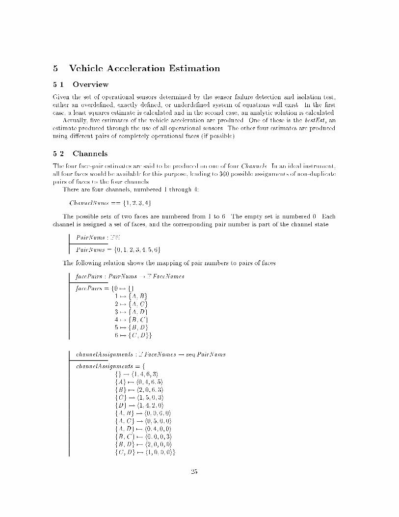
Given the set of operational sensors determined by the sensor failure detection and isolation test,

either an overde�ned, exactly de�ned, or underde�ned system of equations will exist. In the �rst

case, a least squares estimate is calculated and in the second case, an analytic solution is calculated.

Actually, �ve estimates of the vehicle acceleration are produced. One of these is the bestEst , an

estimate produced through the use of all operational sensors. The other four estimates are produced

using di�erent pairs of completely operational faces (if possible).

5.2 Channels

The four face-pair estimates are said to be produced on one of four Channels. In an ideal instrument,

all four faces would be available for this purpose, leading to 360 possible assignments of non-duplicate

pairs of faces to the four channels.

There are four channels, numbered 1 through 4:

ChannelNums == f1; 2; 3; 4g

The possible sets of two faces are numbered from 1 to 6. The empty set is numbered 0. Each

channel is assigned a set of faces, and the corresponding pair number is part of the channel state.

PairNums : FN

PairNums = f0; 1; 2; 3;4; 5; 6g

The following relation shows the mapping of pair numbers to pairs of faces.

facePairs : PairNums ! FFaceNames

facePairs = f0 7! fg

1 7! fA;Bg

2 7! fA;Cg

3 7! fA;Dg

4 7! fB ;Cg

5 7! fB ;Dg

6 7! fC ;Dgg

channelAssignments : F FaceNames ! seqPairNums

channelAssignments = f

fg 7! h1; 4; 6; 3i

fAg 7! h0; 4; 6; 5i

fBg 7! h2; 0; 6; 3i

fCg 7! h1; 5; 0; 3i

fDg 7! h1; 4; 2; 0i

fA;Bg 7! h0; 0; 6; 0i

fA;Cg 7! h0; 5; 0; 0i

fA;Dg 7! h0; 4; 0; 0i

fB ;Cg 7! h0; 0; 0; 3i

fB ;Dg 7! h2; 0; 0; 0i

fC ;Dg 7! h1; 0; 0; 0ig

25

Channels are assigned a set of faces depending upon which faces are nonoperational. The pair

of faces assigned to each of the four channels can be represented as a sequence of pair numbers.

The number of the pair assigned to channel 1 is the �rst value of the sequence, that of channel 2,

the second, and so on. channelAssignments shows the mapping from sets of nonoperational faces to

sequences of pair numbers. For example, if face C is nonoperational then Channel 1 has PairNums

1, Channel 2 has pair 5, Channel 3 has pair 0 (no faces assigned), and Channel 4 has pair 3. Note

that if more than two faces fail, the state of the system is unde�ned.

The schema for a channel is simply:

Channel

status : SystemStatus

acceleration : Vectors3D

chanface : PairNums

and a channel type is:

Channels == fChannelg

The RSDIMU General schema includes a schema FourChannels, which we can now de�ne:

FourChannels

channel : seqChannels

dom channel = ChannelNums

5.3 Basic Calculations

Compensated accelerometer measurements are transformed from the Sensor Frame to the Measure-

ment Frame. Normally, compensated accelerometer measurements are used to make an acceleration

estimate. However, if one sensor on a face has failed, then an uncompensated (Measurement Frame)

measurement is used for the remaining sensor.

The operating sensors being used in any vehicle acceleration estimation (best or channel) each

contribute an equation to the system

�y = C

�

f

I

(4)

where �y is a vector of measuredAccel values for each contributing sensor,

�

f

I

is the unknown force

(acceleration) on the instrument, and C is a matrix representing the transformation from the sensor

frame for each contributing sensor's direction into the instrument frame.

EquationIDs == FaceNames � DirectionNames

Each equation in the system (4) is associated with a particular sensor, which in turn is identi�ed by

a face-direction pair.

DoCreateYmap

�RSDIMU

fnames? : F FaceNames

ymap! : EquationIDs 7! Accelerations

ymap! = � f : FaceNames; d : DirectionNames

j f 2 fnames? ^ d 2 dom face(f ):measuredAccel

� face(f ):measuredAccel(d)

26

The schema is put into a functional form:

createYmap = � fnames : F FaceNames j DoCreateYmap ^ fnames = fnames? � ymap!

Given a set of faces, createYmap returns a relation that maps face names and sensors to ac-

celerometer measurements. Nonoperational sensors do not contribute a measurement value. In the

case of a partially operational face, the value used for the operational sensor is not compensated for

misalignment.

DoCreateCmap

�RSDIMU

fnames? : F FaceNames

map : EquationIDs 7! Vectors3D

cmap! : DirectionNames ! (EquationIDs 7! <)

map = � f : FaceNames; d : SensorNames

j f 2 fnames? ^ : face(f ):sensor(d):linFail

� StoI (f ; d)

cmap! = map

T

The schema is put into a functional form:

createCmap = � fnames : F FaceNames j DoCreateCmap ^ fnames = fnames? � cmap!

Given a set of faces, createCmap returns a relation mapping face names and directions to trans-

formation vectors. As before, nonoperational sensors are not transformed and do not contribute

to the �nal composition of the output set. The entries are obtained from the StoI transformation

de�ned in Section 2.3.3.

Using the building blocks above, we can de�ne functions to be used in calculating the vehicle

acceleration.

AnalyticSolution

�RSDIMU

�Vehicle

�FourChannels

usingFaces? : PFaceNames

acceleration! : Vectors3D

status! : SystemStatus

C : DirectionNames ! (EquationIDs 7! <)

y : EquationIDs 7! Accelerations

C = createCmap(usingFaces?)

y = createYmap(usingFaces?)

#domy = 3

acceleration! = C

�1

y

status! = analytic

world

0

= world

0

v

=

v

�

0

v

= �

v

�

0

v

= �

v

27

LSQSolution

�RSDIMU

�Vehicle

�FourChannels




C : DirectionNames ! (EquationIDs 7! <)


C = createCmap(usingFaces?)


#domy > 3

acceleration! = (C

T

C )

�1

Cy

status! = normal

world

0

= world

0

v

=

v

�

0

v

= �

v

�

0

v

= �

v

Unde�nedSolution

�RSDIMU

�Vehicle

�FourChannels






#domy < 3

acceleration! = zero3D

status! = unde�ned



0


face(f ):linFail

0

= face(f ):linFail ^


0


world

0

= world

0

v

=

v

�

0

v

= �

v

�

0

v

= �

v

These schemas and others to follow assume prior de�nitions of matrix transpose, matrix inverse

and matrix multiplication operations.

AnalyticSolution and LSQSolution return the vehicle acceleration represented in the Instrument

Frame. GetSolution uses whichever of these is applicable, depending upon the number of of equations

in the system 4 (which, in turn, re ects the number of operational sensors within the chosen faces).

28

GetSolution b= LSQSolution _ AnalyticSolution _ Unde�nedSolution

getSolution = � usingFaces : PFaceNames j GetSolution ^ usingFaces? = usingFaces

� (acceleration!; status!)

5.4 Acceleration Estimation

BestEstimateAcceleration

�RSDIMU

�Display

�Vehicle

acc

I

(acc

I

; status

0

) = getSolution(fA;B ;C ;Dg)

acceleration

0

= transform(acc

I

; instrument ; navigation;world) + g

N

world

0

= world

0

v

=

v

�

0

v

= �

v

�

0

v

= �

v

The solution for the acceleration, computed in the instrument frame, must be transformed into the

Navigation Frame and compensated for gravity.

Unde�nedBestEstimate

�RSDIMU

FixedQuantities

�Display

�Vehicle

RSDIMU Unde�ned

status

0

= unde�ned

acceleration

0

= zero3D

29

ChannelEstimateAcceleration

�RSDIMU

�Vehicle

sysStatus

#f f : FaceNames � face(f ):status = nonOperational g � 2

8 c : 1 : : :4 � channel(i):chanface = channelAssignments(nonOpFaces)(c)

8 c : ran channel � 9 acc

I

: Vectors3D �

(acc

I

; c:status

0

) = getSolution(facePairs(c:chanface)) ^

c:acceleration

0

= transform(acc

I

; instrument ; navigation;world) + g

N

^

c:chanface

0

= c:chanface

world

0

= world

0

v

=

v

�

0

v

= �

v

�

0

v

= �

v

sysStatus

0

= sysStatus

acceleration

0

= acceleration

status

0

= status

The solution for each channel is arrived at in a similar manner to the best estimate. The only

real di�erence is in the limited set of faces allowed to getSolution.

Unde�nedChannelEstimate

�RSDIMU

FixedQuantities

�Display

�Vehicle

: sysStatus

8 c : ran channel �

c:status

0

= unde�ned ^

c:acceleration

0

= zero3D

c:chanface

0

= 0

world

0

= world

0

v

=

v

�

0

v

= �

v

�

0

v

= �

v

sysStatus = sysStatus

0

acceleration = acceleration

0

status = status

0

If too many faces are non-operational, the status of the vehicle and the channels is unde�ned , all

acceleration values and chanface values are set to zero.

Finally, EstimateAcceleration is de�ned by:

EstimateAcceleration b= (BestEstimateAcceleration _ Unde�nedBestEstimate)

o

9

(ChannelEstimateAcceleration _ Unde�nedChannelEstimate)

30

Display

Interface

Panel

Display

Control

Words

DMode

Vehicle State

Figure 3: The RSDIMU Display

6 The Display

The display is a component of the Rsdimu that we have largely ignored, to this point. The display

presents any of a number of input, intermediate, and output quantities from the calibration and

estimation processes depending upon the mode setting of the display.

Figure 3 shows the overall structure of the display. Calibration and estimation information,

together with the chosen mode DMODE pass through the DisplayInterface where the quantities to

be displayed are selected and packed into 16-bit words. Individual bits of these words control the

lighting of segments on the DisplayPanel .

ControlWords : P seqZ

8w : ControlWords �

domw = 0 : : 15 ^

ranw � f0; 1g

integerEquiv == �w : ControlWords �

P

15

i=0

w(i) � 2

i

6.1 The Display Panel

Figure 4 shows the layout of the display panel. The panel is divided into three main areas: the mode

indicator, the upper display, and the lower display. The boxes labeled Mi and Di are seven segment

LED (Light-Emitting Diode) displays, whose structure is shown in Figure 5. The Pi are decimal

points and the Si are used to display � signs.

SegmentNames == fA;B ;C ;D ;E ;F ;Gg

segmentOrder == hA;B ;C ;D ;E ;F ;Gi

LED

lit : boolean

voltage : boolean

31

S1

S2

P1 P2 P3 P4 P5 P6

D1 D2 D3 D4 D5

S1

S2

P1 P2 P3 P4 P5 P6

D1 D2 D3 D4 D5

Mode Indicator

Upper Display

Lower Display

M1 M2

Figure 4: The Display Panel

D

G

C

BF

E

A

Figure 5: Seven Segment Displays

32

NegativeLogicLED

LED

lit = : voltage

PositiveLogicLED

LED

lit = voltage

NegativeLogicLEDs = f NegativeLogicLED g

PositiveLogicLEDs = f PositiveLogicLED g

The panel uses a mixture of positive and negative logic LEDs, so that in some cases we must

supply a voltage to light a segment, while in other cases the voltage must be supplied to darken a

segment.

The set of symbols that can be displayed by a seven segment Rsdimu display are:

Symbols == f`0' : : `9'; À' : : `F '; `H '; Ì '; `N '; `P '; ` 'g

symbolOrder == h`0'; `1'; `2'; `3'; `4'; `5'; `6'; `7'; `8'; `9'; À'; `B '; `C '; `D '; È '; `F 'i

A seven segment display can then be described in terms of the segments that must be lit to display

each of these symbols:

SevenSegmentDisplay

segment : SegmentNames ! NegativeLogicLEDs

displaying : Symbols

litSegments : PSegmentNames

litSegments = f s : SegmentNames j segment(s):lit g

displaying = `0') litSegments = fA;B ;C ;D ;E ;Fg

displaying = `1') litSegments = fB ;Cg

displaying = `2') litSegments = fA;B ;D ;E ;Gg

displaying = `3') litSegments = fA;B ;C ;D ;Gg

displaying = `4') litSegments = fB ;C ;F ;Gg

displaying = `5') litSegments = fA;C ;D ;F ;Gg

displaying = `6') litSegments = fA;C ;D ;E ;F ;Gg

displaying = `7') litSegments = fA;B ;Cg

displaying = `8') litSegments = fA;B ;C ;D ;E ;F ;Gg

displaying = `9') litSegments = fA;B ;C ;F ;Gg

displaying = À') litSegments = fA;B ;C ;E ;F ;Gg

displaying = `B ') litSegments = fC ;D ;E ;F ;Gg

displaying = `C ') litSegments = fA;D ;E ;Fg

displaying = `D ') litSegments = fB ;C ;D ;E ;Gg

displaying = È ') litSegments = fA;D ;E ;F ;Gg

displaying = `F ') litSegments = fA;E ;F ;Gg

displaying = `H ') litSegments = fB ;C ;E ;F ;Gg

displaying = Ì ') litSegments = fE ;Fg

displaying = `N ') litSegments = fA;B ;C ;E ;Fg

displaying = `P ') litSegments = fA;B ;E ;F ;Gg

displaying = ` ') litSegments = fg

33

SevenSegmentDisplays == f SevenSegmentDisplay g

The seven segment digit display associates a segment name with each of seven LEDs.

The main task in specifying the control panel is simply to indicate which bits in the incoming

control words control which segment. Because the upper and lower displays are quite similar in this

respect, it is useful to introduce the intermediate concept of a signed 5-digit display.

Signed5DigitDisplay

digits : seq SevenSegmentDisplays

points : seqPositiveLogicLEDs

signs : seqNegativeLogicLEDs

words : seqControlWords

domdigits = 1 : : 5

dompoints = 1 : : 6

dom signs = 1 : : 2

domwords = 1 : : 3

8 i :Z; s : SegmentNames j i 2 1::7 ^ s = segmentOrder(i) �

digits(1)(s):voltage = words(1)(i + 6) ^

digits(2)(s):voltage = words(1)(i � 1) ^

digits(3)(s):voltage = words(2)(i + 6) ^

digits(4)(s):voltage = words(2)(i � 1) ^

digits(5)(s):voltage = words(3)(i � 1)

8 i :Zj i 2 1::6 �

points(i):voltage = words(3)(i + 6)

signs(1):voltage = words(3)(14)

signs(2):voltage = words(3)(13)

Signed5DigitDisplays == f Signed5DigitDisplay g

For example, the seven segments of the leftmost digit are controlled by bits 7 : :13 of the �rst control

word, with segment A controlled by bit 7, segment B by bit 8, and so on.

Similarly, we can describe the mode indicator:

ModeIndicator

modeDigits : seq SevenSegmentDisplay

modeWord : ControlWords

domdigits = 1 : : 2

8 i :Z; s : SegmentNames j i 2 1::7 ^ s = segmentOrder(i) �

modeDigits(1)(s):voltage = modeWord(1)(i + 6) ^

modeDigits(2)(s):voltage = modeWord(1)(i � 1)

With these components, we can describe the display panel.

DisplayPanel

ModeIndicator

upperDisplay : Signed5DigitDisplays

lowerDisplay : Signed5DigitDisplays

34

6.2 The Display Interface

The display interface must map various Rsdimu quantities onto the voltages that will provide the

desired symbols on the panel.

DisplayInterface

DisplayPanel

DMode : 0 : : 99

DisLower ;DisUpper : seqZ

DisMode :Z

domDisLower = domDisUpper = 1 : : 3

8 i :Z�

DisLower(i) = integerEquiv(lowerDisplay :words(i)) ^

DisUpper(i) = integerEquiv(upperDisplay :words(i))

DisMode = integerEquiv(modeWord)

modeDigits(1):displaying = symbolOrder(DMode=10)

modeDigits(2):displaying = symbolOrder(DMode mod 10)

The precise mapping between the vehicle state quantities and the panel depends upon the mode

DMode. In addition, the upper and lower displays can present data in a variety of di�erent formats.

These are presented next.

In the \test" format, all LED's are lit:

TestFormat

Signed5DigitDisplay

8 i :Zj i 2 1 : : 5 �

digits(i):displaying = `8'

8 i :Zj i 2 1 : : 6 �

points(i):lit

signs(1):lit

signs(2):lit

TestFormat5DigitDisplays = f TestFormat g

Similarly, in \blank" format, all LED's must be o�

BlankFormat

Signed5DigitDisplay

8 i :Zj i 2 1 : : 5 �

digits(i):displaying = ` '

8 i :Zj i 2 1 : : 6 �

: points(i):lit

: signs(1):lit

: signs(2):lit

BlankFormat5DigitDisplays = f BlankFormat g

35

In \failure" mode, the �rst digit shows a face name, the second is blank, the third shows the

status of the face's x sensor, the fourth is blank, and the �fth shows the status of the face's y sensor.

faceToNameMap == fA 7! À';B 7! `B ';C 7! `C ';D 7! `D 'g

failureIndicator : Sensors ! Symbols

8 s : Sensors j : s:linFail � failureIndicator(s) = `P '

8 s : Sensors j s:linNoise � failureIndicator(s) = `N '

8 s : Sensors j s:prevFailed � failureIndicator(s) = Ì '

8 s : Sensors j : (s:linFail _ s:linNoise _ s:prevFailed) � failureIndicator(s) = `F '

The function failureIndicator returns `P' for operational sensors, `N' for sensors rejected due to

excessive noise, Ì' for sensors marked as failed upon input (prior to calibration), and `F' for sensors

that fail during the edge-vector test.

FailureFormat

Signed5DigitDisplay

faceToCheck : Faces

digits(1):displaying = faceToNameMap(faceToCheck :sensorFrame)

digits(2):displaying = digits(4):displaying = ` '

digits(3):displaying = failureIndicator(faceToCheck :sensor(x ))

digits(5):displaying = failureIndicator(faceToCheck :sensor(y))

8 i :Zj i 2 1 : : 6 � : points(i):lit

: signs(1):lit

: signs(2):lit

FailureFormat5DigitDisplays = � f : Faces j f = faceToCheck � FailureFormat

In \hexadecimal" format, the display presents an integer quantity as a hexadecimal number.

HexFormat

Signed5DigitDisplay

k :Z

digits(1):displaying = `H '

8 i :Zj i 2 2 : : 5 �

digits(i):displaying = symbolOrder(

�

k

16

5�i

mod 16

�

+ 1)

8 i :Zj i 2 1 : : 6 � : points(i):lit

: signs(1):lit

: signs(2):lit

HexFormat5DigitDisplays = � i :Zj i = k � HexFormat

In \signed decimal" format, the display presents a real number in a �xed point format. The

requirements document [1] explicitly speci�es several subranges:

36

SignedDecimalLow

Signed5DigitDisplay

r : <

r < �99999:0

: signs(1):lit

signs(2):lit

points(6):lit

8 i :Zj i 2 1 : : 5 � : points(i):lit

8 i :Zj i 2 1 : : 5 � digits(i):displaying = `9'

SignedDecimalHigh

Signed5DigitDisplay

r : <

r > 99999:0

signs(1):lit

signs(2):lit

points(6):lit

8 i :Zj i 2 1 : : 5 � : points(i):lit


SignedDecimalNearZero

Signed5DigitDisplay

r : <

�0:000005 < r < 0:000005

: signs(1):lit

: signs(2):lit

points(1):lit

8 i :Zj i 2 2 : : 6 � : points(i):lit


37

SignedDecimalPositive

Signed5DigitDisplay

r : <

ptPos :Z

norm :Z

0:000005 � r � 99999:0

signs(1):lit

signs(2):lit

ptPos = max(1; 2 + log

10

r)

norm = trunc(0:5 + r � (4 � log

10

r))

points(ptPos):lit

8 i :Zj i 2 1 : : 6 ^ i 6= ptPos �

: points(i):lit

8 i :Zj i 2 1 : : 5 �


norm

10

5�i

mod10+1

)

SignedDecimalNegative

Signed5DigitDisplay

r : <

ptPos :Z

norm :Z

�99999:0 � r � �0:000005

: signs(1):lit

signs(2):lit

ptPos = max(1; 2 + log

10

(�r))

norm = trunc(0:5 + r � (4 � log

10

(�r)))

points(ptPos):lit

8 i :Zj i 2 1 : : 6 ^ i 6= ptPos �

: points(i):lit

8 i :Zj i 2 1 : : 5 �


norm

10

5�i

mod10+1

)

SignedDecimalFormat b= SignedDecimalLow _ SignedDecimalHigh _ SignedDecimalNearZero

_ SignedDecimalPositive _ SignedDecimalNegative

SignedDecimalFormat5DigitDisplays = � q : < j r = q � SignedDecimalFormat

With the various formats speci�ed, we can now enumerate the various modes of the display

interface.

38

TestMode

DisplayInterface

DMode = 88

upperDisplay 2 TestFormat5DigitDisplays

lowerDisplay 2 TestFormat5DigitDisplays

BlankMode

DisplayInterface

DMode 2 f0; 5 : : 20; 25 : : 30; 34 : : 87; 89 : : 99g

upperDisplay 2 BlankFormat5DigitDisplays

lowerDisplay 2 BlankFormat5DigitDisplays

faceOrders : seqFaceNames

faceOrders = hA;B ;C ;Di

FailureMode

DisplayInterface

faces : FaceNames ! Faces

faceToCheck : FaceNames

DMode 2 1 : : 4

faceOrders(faceToCheck) = DMode

upperDisplay 2 BlankFormat5DigitDisplays

lowerDisplay 2 FailureFormat5DigitDisplays(faces(faceToCheck))

RawlMode

DisplayInterface

faces : FaceNames ! Faces

faceToCheck : FaceNames

DMode 2 21 : : 24

faceOrders(faceToCheck) = DMode + 20

upperDisplay 2 HexFormat5DigitDisplays(face(faceToCheck):sensor(x ):rawl)

lowerDisplay 2 HexFormat5DigitDisplays(face(faceToCheck):sensor(y):rawl)

dirOrders : seqDirectionNames

dirOrders = hx ; y ; z i

39

BestEstMode

DisplayInterface

bestEst : Vectors3D

dirToCheck : DirectionNames

DMode 2 31 : : 33

dirOrders(dirToCheck) = DMode + 30

upperDisplay 2 SignedDecimalFormat5DigitDisplays(bestEst :x )

lowerDisplay 2 BlankFormat5DigitDisplays

These modes combine to form the complete speci�cation of the display unit.

Display b= TestMode _ BlankMode _ FailureMode

_ RawlMode _ BestEstMode

It is worth noting that the entire Display has been de�ned in terms of invariants on the rest of

the Rsdimu. There are no state transitions on the display. The display is presumed to continuously

show the quantities in the Rsdimuselected by the DMode. The requirements further specify that

DMode is �xed during the period of time covered by this speci�cation (calibration followed by a

single in- ight reading).

7 Initialization

Because the requirements for the Rsdimu postulate a driver program that supplies a valid initial

state, there is no need for an initialization schema in the usual sense (i.e., for constructing a valid

Rsdimu state as a base case). We do, however, need to be concerned with the initialization of

quantities introduced in this speci�cation but not explicitly contained in [1]. This initialization can

postulate a prior valid state.

40

InitRSDIMU

�RSDIMU


face(f ):sensor(d):prevFailed

0

= face(f ):sensor(d):linFail (5)

world

0

= world

0

I

=

I

�

0

I

= �

I

�

0

I

= �

I

obase

0

= obase

8 f : FaceNames �

(face(f ):sensorFrame

0

= face(f ):sensorFrame ^

face(f ):misalign

0

= face(f ):misalign ^

face(f ):temp

0

= face(f ):temp ^

face(f ):normFace

0

= face(f ):normFace)


(face(f ):o�Raw

0

= face(f ):o�Raw ^


0



0



0


face(f ):sensor(d):rawl

0

= face(f ):sensor(d):rawl ^


0

= face(f ):sensor(d):linNoise ^

face(f ):sensor(d):linO�set

0

= face(f ):sensor(d):linO�set ^

face(f ):sensor(d):linFail

0

= face(f ):sensor(d):linFail)

DMode

0

= DMode

The only real point of interest here is equation 5, which indicates that prevFailed holds the sensor

failure information prior to our beginning any calibration activities. (It corresponds therefore to the

value of the variable LINFAILIN in [1].

8 Conclusions

The Rsdimu project was selected to give students experience in the process of writing formal speci�-

cations for a realistic project. Without this experience, students are often inclined to dismiss formal

methods as having low relevance outside of academia. The small examples that �ll most textbooks,

useful as they are for pedagogical purposes, do little to dispell this prejudice. Even the longer case

studies from [2] are insu�ciently convincing. For example, none of the case studies in [2] illustrate

the use of multiple layers of Z-de�ned abstract objects (except in one-to-one containment), which

proved so important in this speci�cation.

The Rsdimu requirements were useful because they were clearly authentic, and because they

were involved enough to be quite intimidating at the start of the project. Student comments at the

end of the semester indicated that they were, in fact, surprised at how much they had been able to

accomplish in a relatively short period of time.

41

References

[1] Charles Rivers Analytics, Inc. Redundancy management software: Requirements spec-

i�cation for a redundant strapped down inertial measurement unit. Technical Report

NASA.FTS87/RSDIMU/RS/3.2/Feb-87, NASA, Feb. 1987. Version 3.2.

[2] A. Diller. Z { an Introduction to Formal Methods. John Wiley & Sons, 1990.

[3] D. E. Eckhardt, A. K. Caglayan, J. C. Knight, L. D. Lee, D. F. McAllister, M. A. Vouk, and

J. P. J. Kelly. An experimental evaluation of software redundancy as a strategy for improving

reliability. IEEE Transactions on Software Engineering, 17(7):692{702, July 1991.

[4] P. R. Lorczak and A. K. Caglayan. A large scale second generation experiment in multi-version

software: Analysis of software and speci�cation errors. Technical Report R8903, Charles River

Analytics, Inc., Jan. 1989.

42

Index

acceleration, 15, 18, 19, 22{24, 26, 29, 30

Accelerations, 11, 11, 13, 26{28

AnalyticSolution, 27, 29

AtoI, 9, 14

bad, 21, 21, 24

BestEstimateAcceleration, 29, 30

BestEstMode, 40, 40

BlankFormat5DigitDisplays, 35, 39

BlankMode, 39, 40

BtoI, 9, 14

Calibration, 24

chanface, 26, 30

channel, 26, 30

channelAssignments, 25, 30

ChannelEstimateAcceleration, 30, 30

ChannelNums, 25, 26

CheckFailingFace, 23, 24

CheckForNoise, 19, 24

CheckPartialFaceX, 23, 24

CheckPartialFaceY, 23, 24

checkSensorsInFace, 24, 24

ControlWords, 31, 31, 34

coord, 5, 5, 6, 13, 14, 18, 22

Counts, 11, 11, 18

createCmap, 27, 27, 28

createYmap, 27, 27, 28

CtoI, 9, 14

�, 20

DetermineO�sets, 18, 24

DirectionNames, 4, 4, 8, 11, 18, 26{28, 39, 40

Directions, 5

Display, 15, 24, 29, 30, 40

DisplayInterface, 35, 39, 40

DisplayPanel, 34, 35

DMode, 35, 39{41

DtoI, 9, 14

EdgeNames, 20, 21, 24

Edges, 21, 21

EdgeSet, 15, 21

EquationIDs, 26, 26, 27, 28

EstimateAcceleration, 30

face, 14, 15{21, 23, 24, 26{28, 30, 39, 41

FaceCompletelyOperational, 24, 24

faceFailsEdgeTest, 21, 23

FaceNames, 12, 13, 14, 16{30, 39, 41

FaceNonOperational, 24, 24

faceOrders, 39

facePairs, 25, 30

FacePartiallyOperational, 24, 24

Faces, 14, 14, 36, 39

FaceStatus, 12, 13

faceToNameMap, 36, 36

FailureFormat5DigitDisplays, 36, 39

failureIndicator, 36, 36

FailureMode, 39, 40

FixedQuantities, 17, 18, 19, 23, 24, 29, 30

FourChannels, 15, 26, 27, 28

Frames, 5, 5, 6, 7, 10, 12, 13, 18, 19

fromMisaligned, 8, 13

g

N

, 10

getSolution, 29, 29, 30

HexFormat5DigitDisplays, 36, 39

identity, 4, 4{6

InitRSDIMU, 41

Instrument, 14, 15

integerEquiv, 31, 35

IsolateSensorFailures, 24, 24

ItoA, 9, 14

ItoB, 10, 14

ItoC, 10, 14

ItoD, 10, 14

LED, 31, 33

lin, 11

linFail, 11, 11, 14, 16, 18{20, 23, 27, 28, 36,

41

linNoise, 11, 18, 19, 23, 24, 28, 36, 41

linO�set, 11, 18, 19, 23, 24, 28, 41

linstd, 11, 11, 19, 20

lit, 31, 33, 35{38

lowerDisplay, 34, 35, 39, 40

LSQSolution, 28, 29

measuredAccel, 13, 13, 14, 26

measureFor, 10, 13, 18, 19, 22

measurementFrame, 13, 14

misalign, 13, 17, 41

MisalignmentAngles, 8, 8, 13

43

MisalignmentNames, 8, 13

modeDigits, 34, 34, 35

ModeIndicator, 34, 34

modeWord, 34, 35

NegativeLogicLEDs, 33, 33, 34

nonOpFaces, 14, 30

normFace, 13, 13, 17, 41

obase, 14, 17, 41

o�Raw, 11, 11, 17{19, 41

PairNums, 25, 25, 26

Points, 5, 6, 7, 13, 17, 21

PositiveLogicLEDs, 33, 34

prevFailed, 11, 11, 17, 36, 41

rawl, 11, 17, 39, 41

RawlMode, 39, 40

rotate, 10, 13, 15

rotation, 5, 6, 9, 10

RSDIMU, 16, 17{24, 26{30, 41

RSDIMUGeneral, 15, 16, 21

SegmentNames, 31, 34

segmentOrder, 31, 34

sensorDeviatesFromLSQ, 22, 23

sensorFrame, 13, 17, 36, 41

SensorNames, 11, 13, 14, 16{20, 22{24, 27, 28,

41

Sensors, 12, 13, 36

sensors, 13, 13

SevenSegmentDisplays, 34, 34

Signed5DigitDisplays, 34, 34

SignedDecimalFormat5DigitDisplays, 38, 40

speci�cForce, 11, 11, 13, 22

speci�cForceMF, 13, 13, 14

speci�cForceSF, 13, 13, 21

status, 13, 13, 14, 15, 16, 21, 23, 24, 26, 29,

30

symbolOrder, 33, 35, 36, 38

Symbols, 33, 33, 36

sysStatus, 15, 18, 19, 24, 30

system, 5, 6

SystemStatus, 15, 15, 26{28

Temperatures, 11, 11, 13

TestFormat5DigitDisplays, 35, 39

TestMode, 39, 40

toMisaligned, 8, 13

transform, 6, 6, 7, 13, 17, 22, 29, 30

Transformations, 5, 6

TransformMatrices, 4, 4, 5{10

translation, 5, 6, 9, 10, 18, 19

Unde�nedBestEstimate, 29, 30

Unde�nedChannelEstimate, 30, 30

Unde�nedSolution, 28, 29

upperDisplay, 34, 35, 39, 40

Vectors3D, 4, 4, 5, 6, 8, 10, 15, 26{28, 30, 40

Vehicle, 15, 15, 27{30

voltage, 31, 33, 34

world, 13, 14, 15, 17{19, 22, 27{30, 41

Worlds, 6, 6, 7, 13{15

zero3D, 4, 5, 5, 6, 28{30

44

ts ten con - old dominion universitytkennedy/cs350/sum15/public/reqts/...purp ose this sensor y arra...

Documents