Tropical Cyclone Axisymmetric Physics

Tropical Cyclone Axisymmetric Physics

Kerry EmanuelLorenz Center, MIT

Program

Brief Overview

Steady-state energetics and physics

Structure

Intensification physics

Overview: What is a Tropical Cyclone?

A tropical cyclone is a nearly symmetric, warm-core cyclone powered by wind-induced enthalpy fluxes from the sea surface

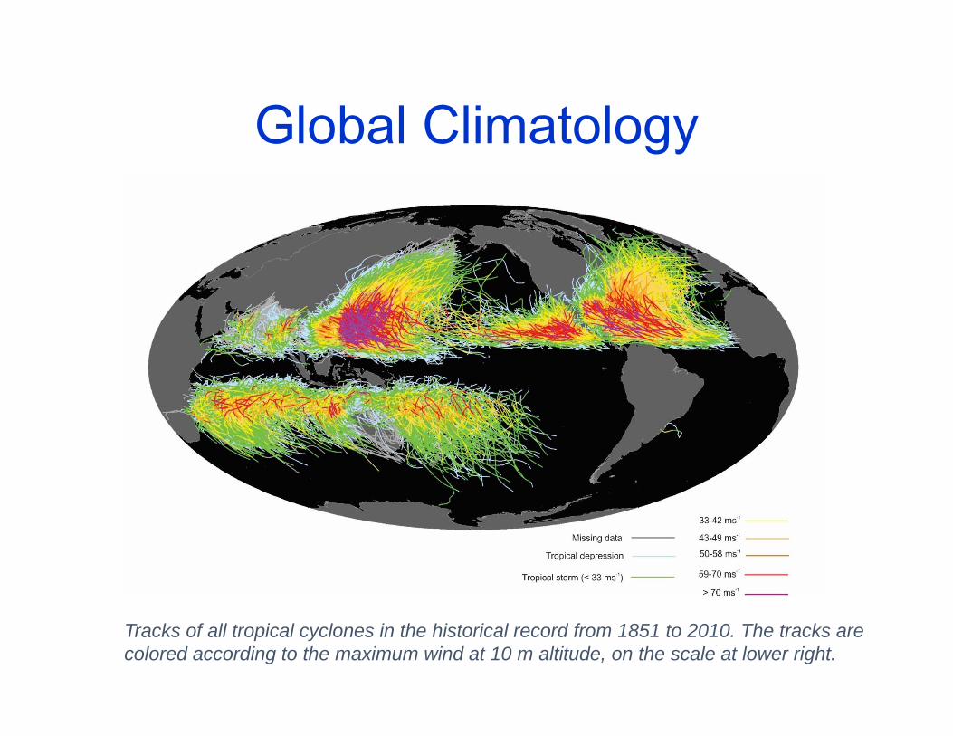
Global Climatology

Tracks of all tropical cyclones in the historical record from 1851 to 2010. The tracks are colored according to the maximum wind at 10 m altitude, on the scale at lower right.

The View from Space

View of the eye of Hurricane Katrina on August 28th, 2005, as seen from a NOAA WP-3D hurricane

reconnaissance aircraft.

Hurricane Structure: Wind Speed

Azimuthal component of wind< 11 5 ms-1 - > 60 ms-1

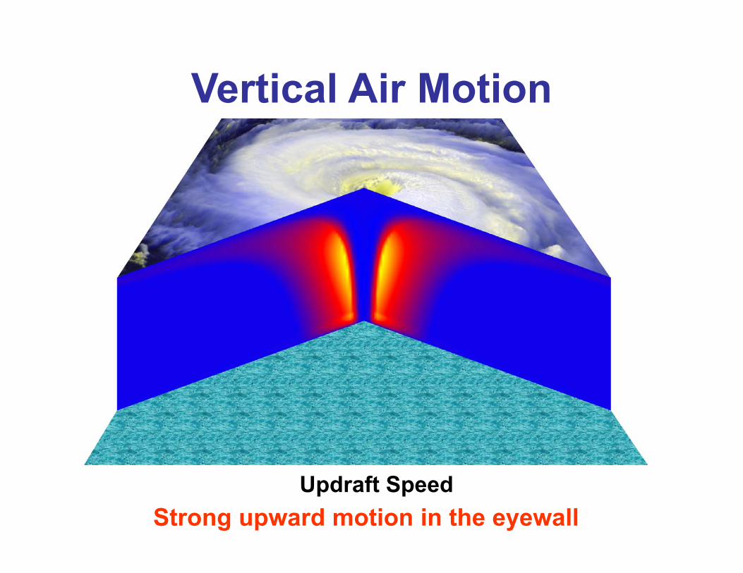
Updraft Speed

Vertical Air Motion

Strong upward motion in the eyewall

Specific entropy

Absolute angular momentum per unit mass2M rV r

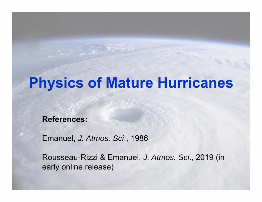
Physics of Mature Hurricanes

References:

Emanuel, J. Atmos. Sci., 1986

Rousseau-Rizzi & Emanuel, J. Atmos. Sci., 2019 (in early online release)

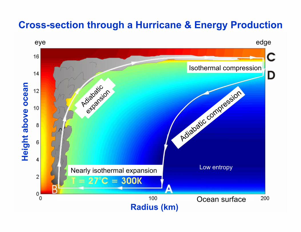
Cross-section through a Hurricane & Energy Production

Nearly isothermal expansion

Isothermal compression

eye edge

Low entropy

Hei

ght a

bove

oce

an

Ocean surfaceRadius (km)

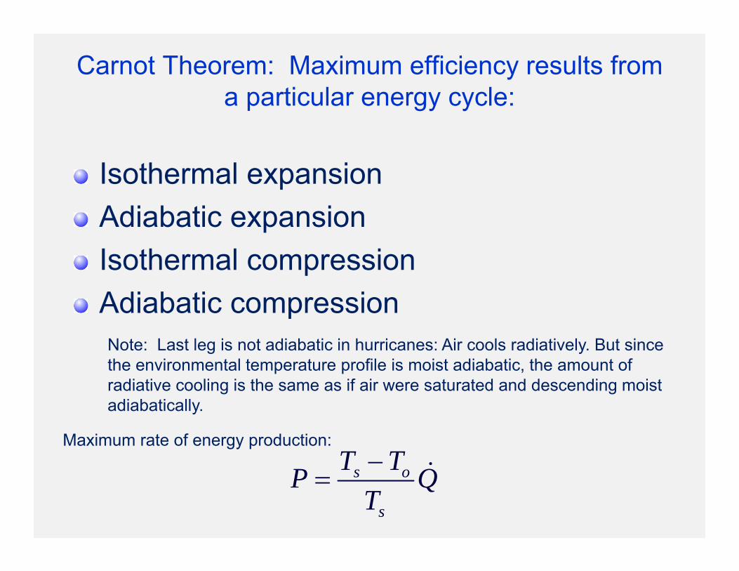
Carnot Theorem: Maximum efficiency results from a particular energy cycle:

Isothermal expansionAdiabatic expansionIsothermal compressionAdiabatic compressionNote: Last leg is not adiabatic in hurricanes: Air cools radiatively. But since the environmental temperature profile is moist adiabatic, the amount of radiative cooling is the same as if air were saturated and descending moist adiabatically.

Maximum rate of energy production:

s o

s

T TP QT

Total rate of heat input to hurricane:

0 * 300

2 | | | |r

k DQ C k k C rdr V V

Surface enthalpy flux Dissipative heating

In steady state, energy production is used to balance frictional dissipation:

0 3

02 | |

r

DD C rdr V

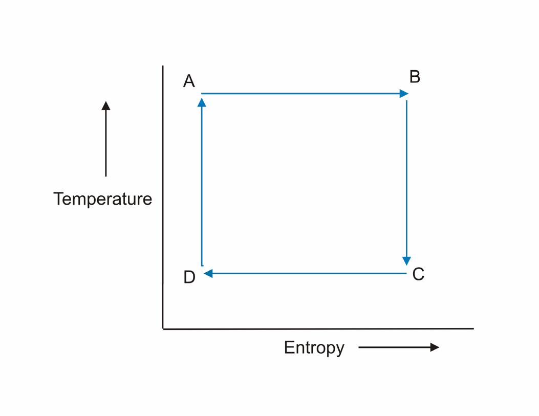
Differential Carnot Cycle

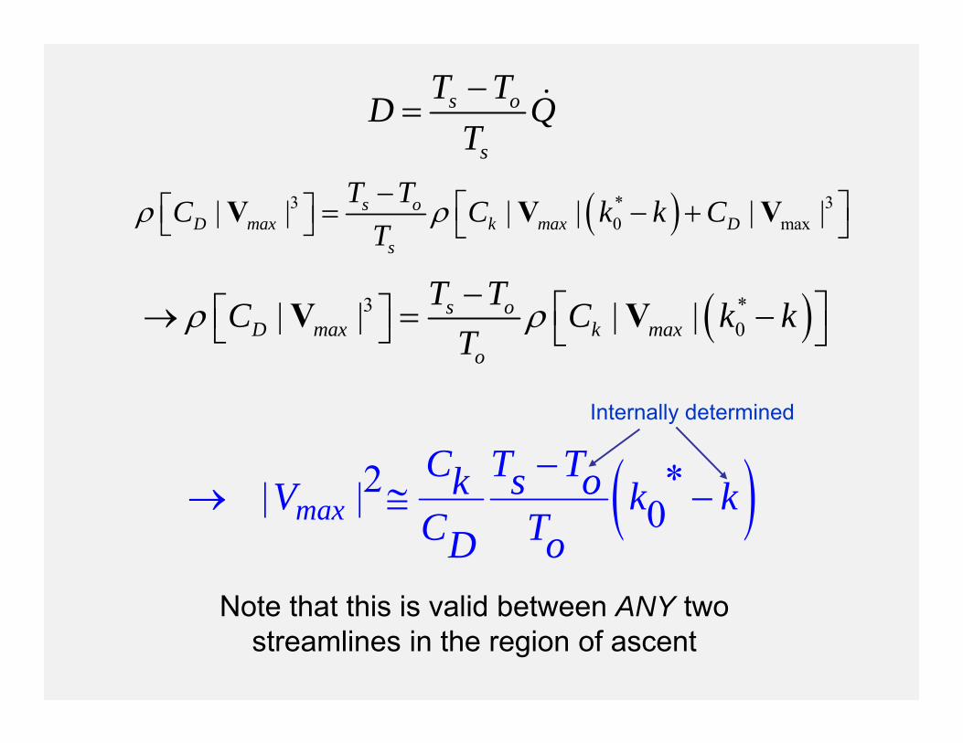
3 *0| | | |s o

D ko

max maxT TC C k k

T V V

2 *| | 0maxC T Tk s oV k kC TD o

s o

s

T TD QT

Note that this is valid between ANY two streamlines in the region of ascent

Internally determined

3 * 30 max| | | | | |s o

D k Dmaxs

maxT TC C k k C

T V V V

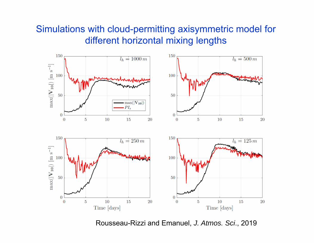
Simulations with cloud-permitting axisymmetric model for different horizontal mixing lengths

Rousseau-Rizzi and Emanuel, J. Atmos. Sci., 2019

Derivation of gradient wind potential intensity from thermal wind balance

2 22

3

14

g gV MfV f r

r r r

Gradient balance

p

Hydrostatic balance

3

2 ** p

g gM M sr p r s r

212g gM rV rf

Thermal wind

3*

2 *

s

g g g

g

M M MT dsr p p dM r

3*

2 *

s

g g g

g

M M MT dsr p p dM r

*3

1 1 *2

gM sg g

r ds Tr p M dM p

Integrate in pressure:

2 2

*g gb o

b go

M M dsT Tr r dM

*gb

b g

gob o

o

V V dsT Tr r dM

(1)

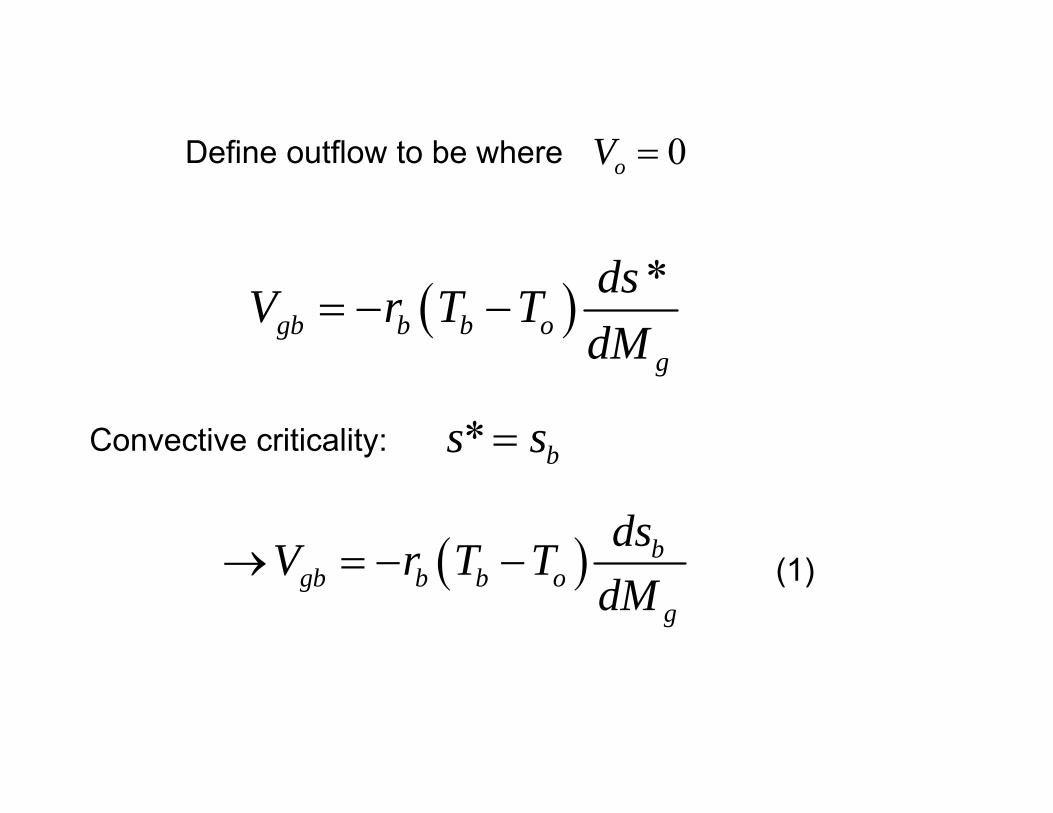
*b

ggb b o

dsV r T TdM

Convective criticality: * bs s

g

bgb b b o

dsV r T TdM

(1)

Define outflow to be where 0oV

dsb /dMg determined by boundary layer processes

Put (1) in differential form:

Integrate entropy equation through depth of boundary layer:

(2)

(3)

Integrate angular momentum equation through depth of boundary layer:

(4)

03*1 | | | |k D

s

dsh C k k Cdt T

V V

2 0.g gb o

M dMdsT Tdt r dt

| |gD

dMdMh h C rVdt dt

V

Substitute (3) and (4) into (2) and equate

2 *| | 0C T Tk s o k kC TD o

V (5)

Same answer as from Carnot cycle. This is still not a closed expression, since we have not determined the boundary layer enthalpy, k or the outflow temperature, To

| |:V Vwith

What Determines Outflow Temperature?

Reference: Emanuel and Rotunno, J. Atmos. Sci., 2011

Simulations with Cloud-Permitting, Axisymmetric Model

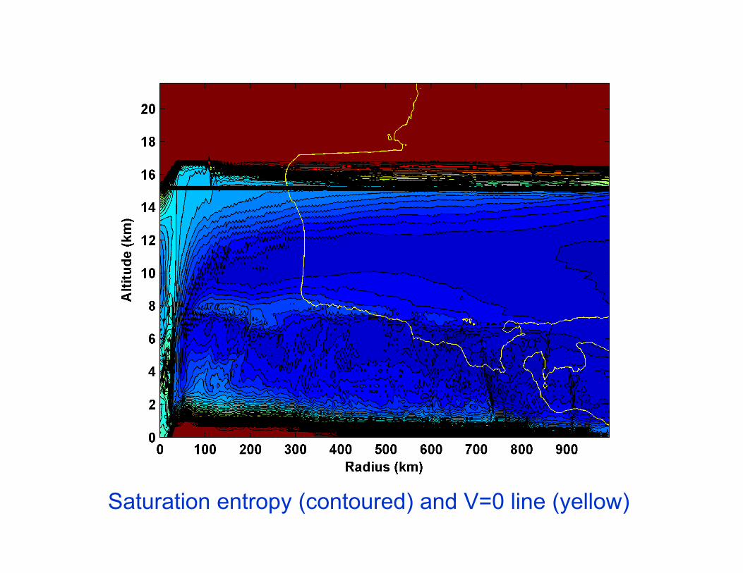
Saturation entropy (contoured) and V=0 line (yellow)

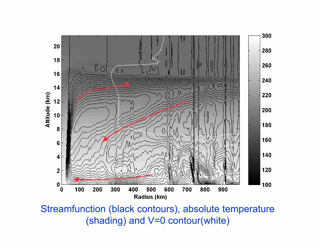
Streamfunction (black contours), absolute temperature (shading) and V=0 contour(white)

Angular momentum surfaces plotted in the V-T plane. Red curve shows shape of balanced M surface originating at radius of maximum winds. Dashed red line is ambient

tropopause temperature.

Richardson Number (capped at 3). Box shows area used for scatter plot.

Vertical Diffusivity (m2s-1)

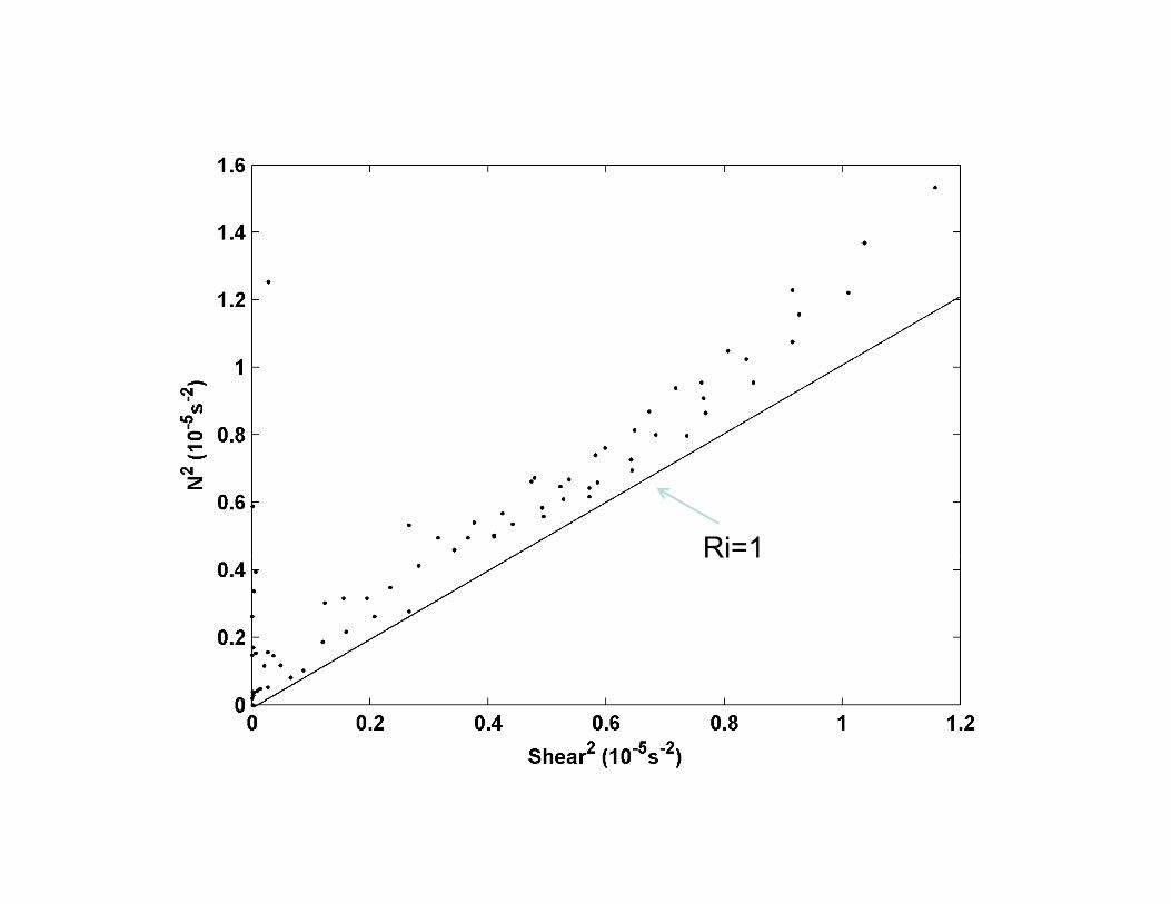
Ri=1

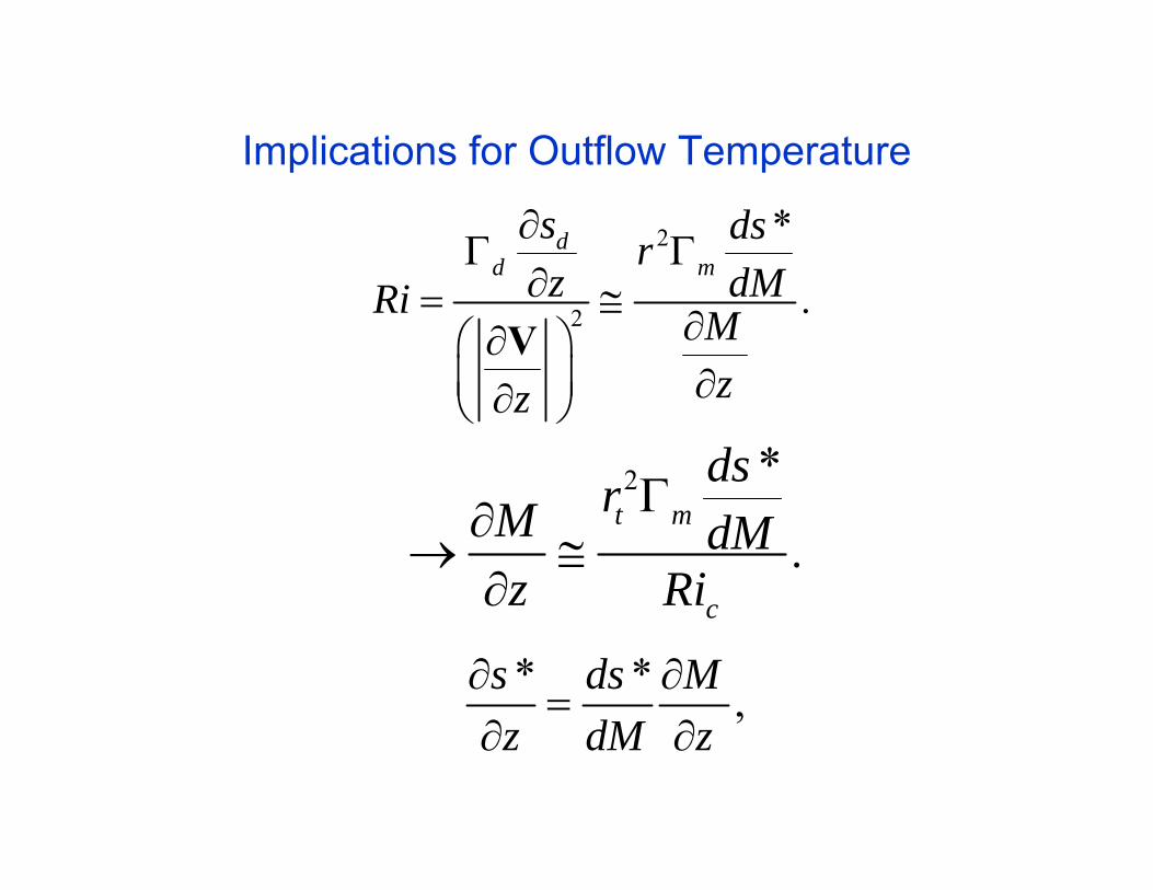
2

2 *

.d

d ms dsrz dMRi M

zz

V

2 *

.t m

c

dsrM dMz Ri

* * ,s ds Mz dM z

Implications for Outflow Temperature

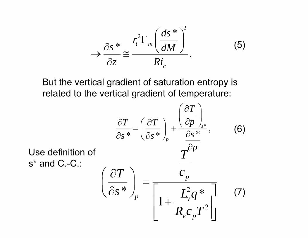
22 *

* .t m

c

dsrs dMz Ri

But the vertical gradient of saturation entropy is related to the vertical gradient of temperature:

* ,** *s

p

TpT Tss sp

2

2

* *1

p

p v

v p

TcT

s L qR c T

Use definition of s* and C.-C.:

(6)

(7)

(5)

2

2

.** *1

p m

v

v p

TcT

ss L qzR c T

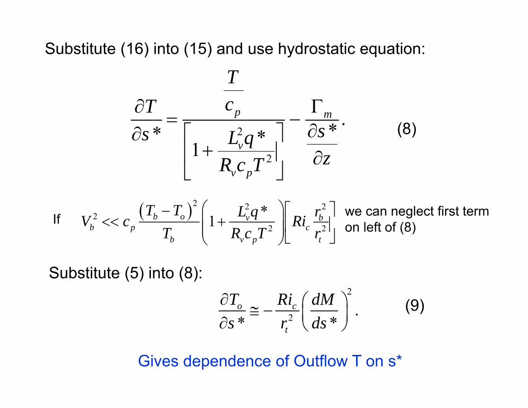
Substitute (16) into (15) and use hydrostatic equation:

Substitute (5) into (8):2

2 .* *o c

t

T Ri dMs r ds

Gives dependence of Outflow T on s*

2 2 22

2 2

*1b o v bb p c

b v p t

T T L q rV c RiT R c T r

If

(8)

(9)

we can neglect first term on left of (8)

,* *

T T dMs M ds

2 .*

o c

t

T Ri dMM r ds

Using

We can re-write (9) as (10)

2 1 *2b b b o

dsM r f T TdM

We can also re-write (1) as

(11)

3

*0

| || |bk b d

b

dsh C s s Cdt T

VVBoundary layer

entropy:(12)

| |dMh r Vdt

VBoundary layer angular momentum: (13)

Combine (12) and (13):

* 20 | |bb k

D b

s sds CdM C rV T rV

V

Let *, | | ,b b bs s V V r rV

*0 ** k b

D b b b b

s sds C VdM C rV T r

Balance condition (1):

*bb o

b

V dsT Tr dM

(14)

(15)

Eliminate Vb between (14) and (15):

*20

2

** b k

o D b b o

s sds T CdM T C r T T

Eliminate rb2 between (11) and (16):

2* *2 0,b o

ds ds fdM dM T T

where 0 * *2

b k

o D

T C s sT C M

Remember that2 *

o c

t

T Ri dMM r ds

(16)

(17)

(10)

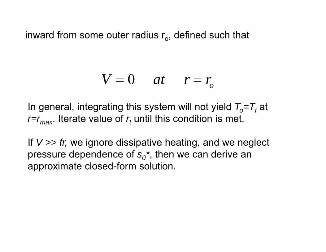
inward from some outer radius ro, defined such that

0 oV at r r

In general, integrating this system will not yield To=Tt at r=rmax. Iterate value of rt until this condition is met.

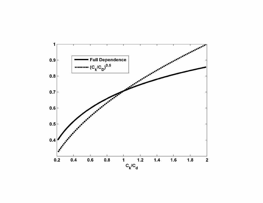
If V >> fr, we ignore dissipative heating, and we neglect pressure dependence of s0*, then we can derive an approximate closed-form solution.

2

2

2

2,

2

k

D

CC

m

m k k

D D m

rrM

M C C rC C r

Assuming that Ri is critical in the outflow leads to an equation for To that, coupled to the interior balance equation and the slab boundary layer lead (surprisingly!) to a closed form analytic solution for the gradient wind (as represented by angular momentum, M, at the top of the boundary layer:

(18)

2

22

2

2.

22

k

D

oCC

mo

m m k k o

D D m

rrfr

V r C C rC C r

1

22 11 12 2

k

D

Ck C

m o mD

Cr fr VC

22

2

2k

kD

D

CC CC m

m po

rV Vfr

The maximum wind speed,     , found from maximizing the radial dependence of wind speed in the solution (18) on previous slide is given by

mV

(19)

(20)

(21)

Evaluate at ro:

For :o mr r

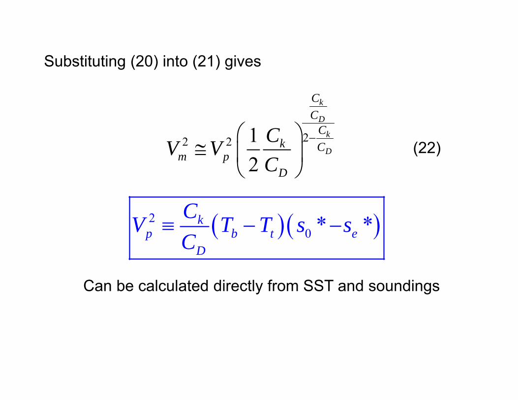
20 * *k

p b t eD

CV T T s sC

22 2 12

k

D

k

D

CC

Ck C

m pD

CV VC

Can be calculated directly from SST and soundings

Substituting (20) into (21) gives

(22)

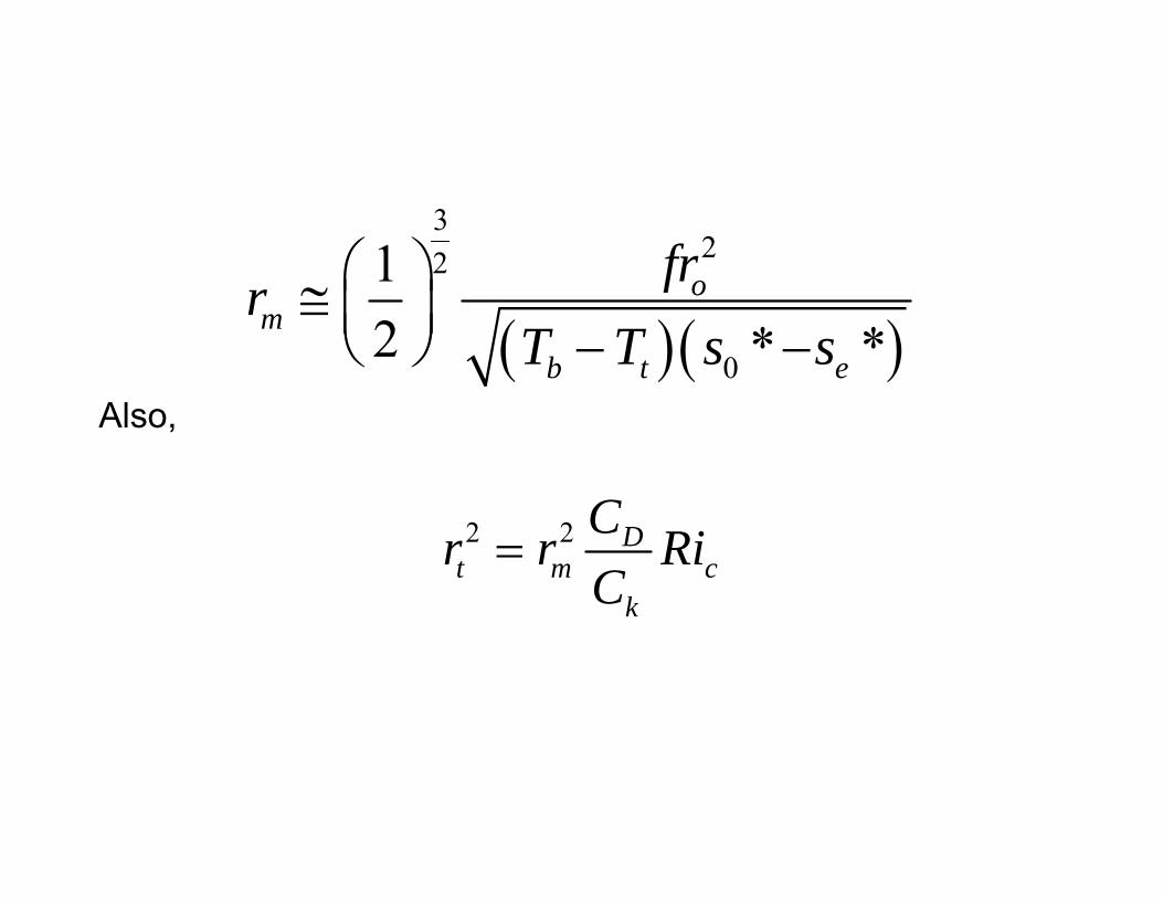
322

0

12 * *

om

b t e

frrT T s s

2 2 Dt m c

k

Cr r RiC

Also,

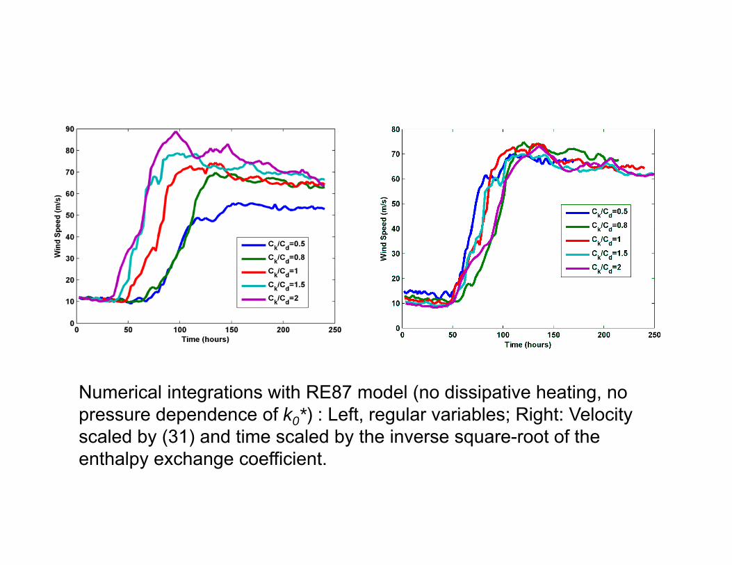
Numerical integrations with RE87 model (no dissipative heating, no pressure dependence of k0*) : Left, regular variables; Right: Velocity scaled by (31) and time scaled by the inverse square-root of the enthalpy exchange coefficient.

Effects of Pressure-Dependence of Surface Saturation Enthalpy

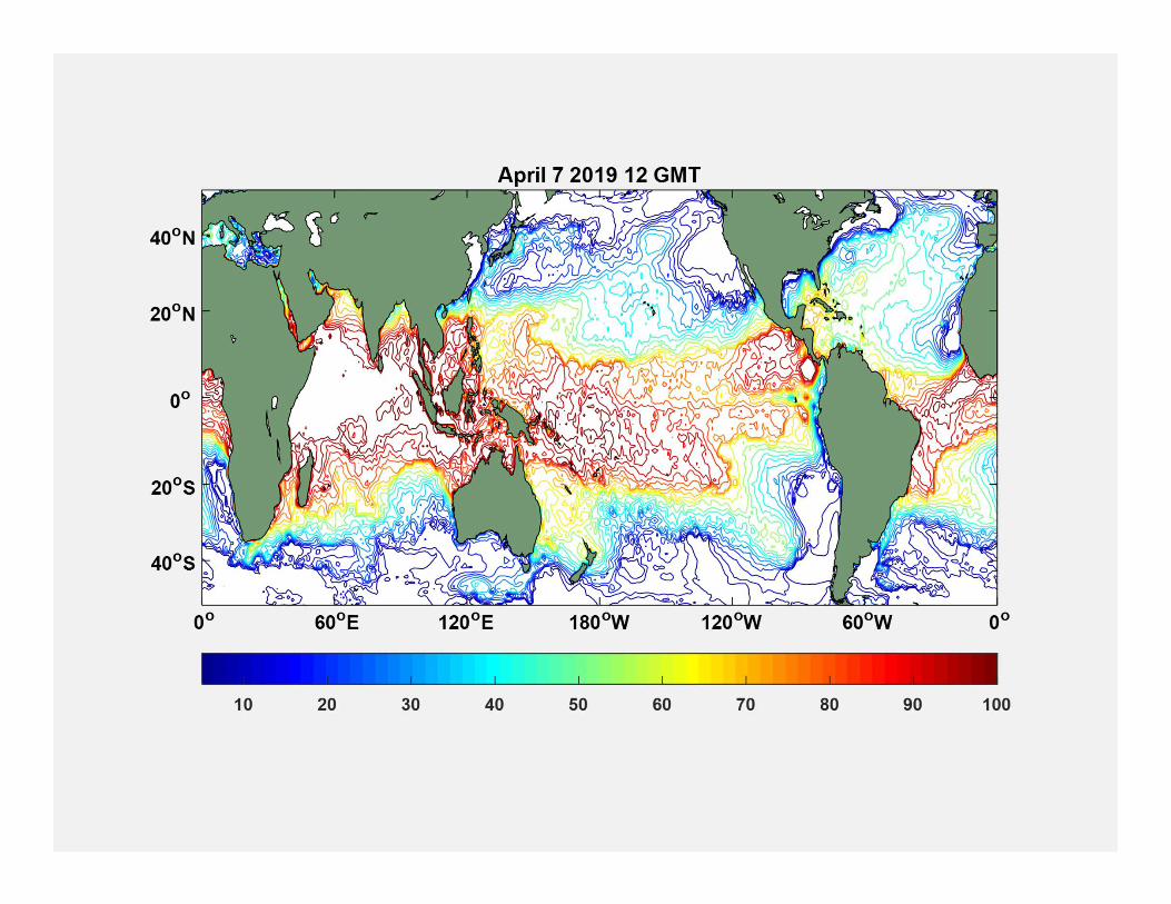
0o 60oE 120oE 180oW 120oW 60oW

60oS

30oS

0o

30oN

60oN

0 10 20 30 40 50 60 70 80

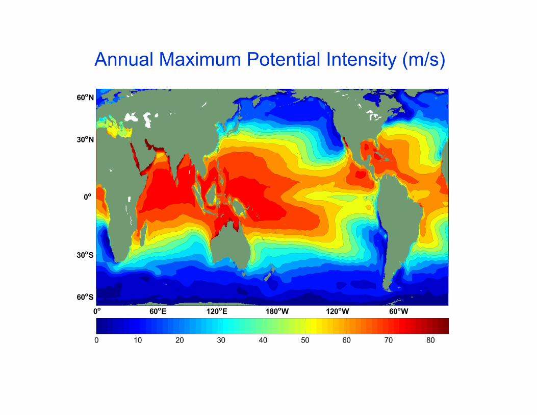
Annual Maximum Potential Intensity (m/s)

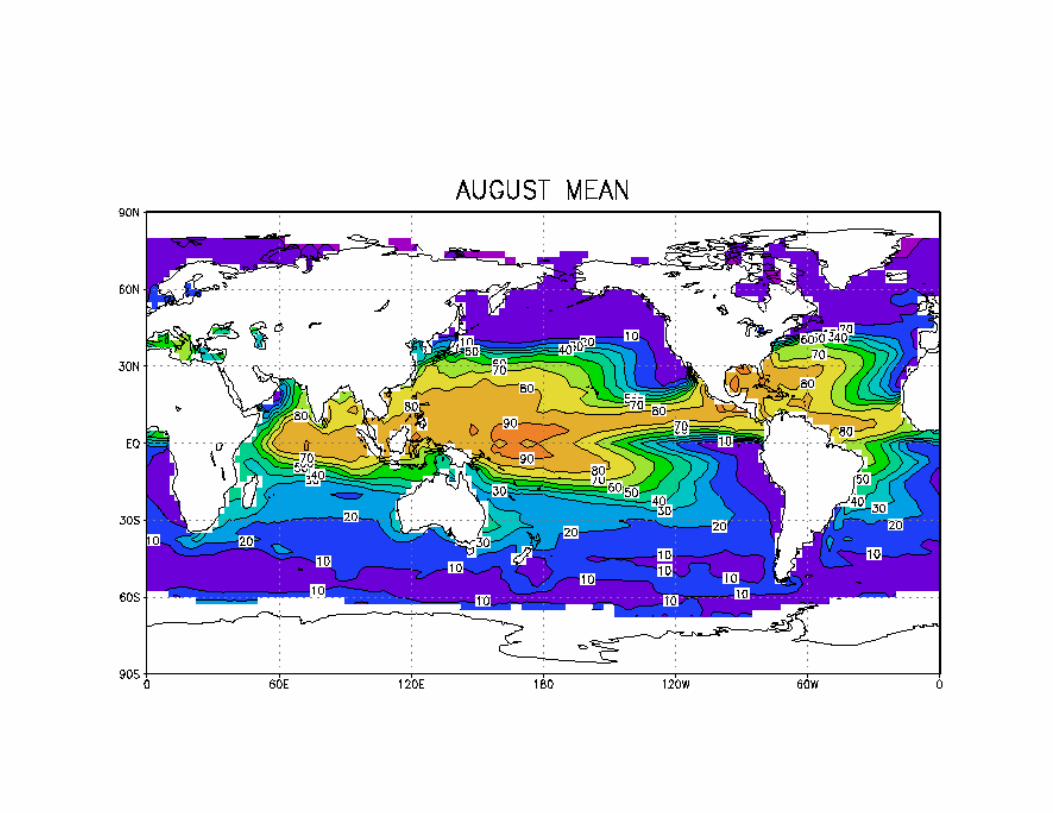
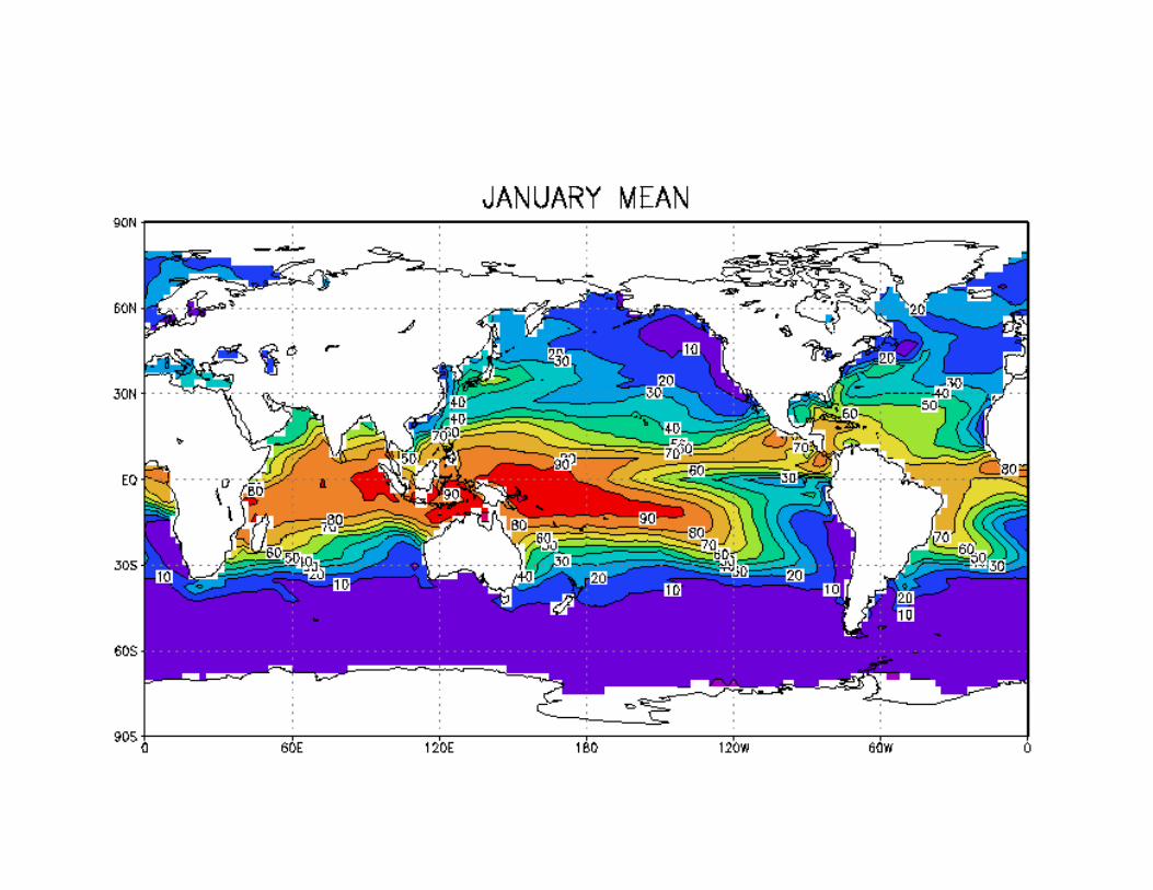
Thermodynamic disequilibrium is necessary to maintain ocean heat balance:

Ocean mixed layer Energy Balance (neglecting lateral heat transport):

*0| |k entrainC k k F F F

sV

2

| |entrains o

po D s

F F FT TVT C

V

Greenhouse effect decreases this

Mean surface wind speedWeak explicit

dependence on Ts

Ocean mixed layer entrainment

Dependence on Sea Surface Temperature (SST):

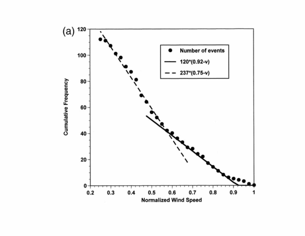
Relationship between potential intensity (PI) and intensity of

real tropical cyclones

(Following slides from Emanuel, K.A., 2000: A statistical analysis of hurricane intensity. Mon. Wea. Rev., 128, 1139-1152.)