tree automata techniques and applications
TRANSCRIPT

TreeAutomataTechniques andApplications
Hubert Comon Max Dauchet Remi GilleronFlorent Jacquemard Denis Lugiez Sophie Tison
Marc Tommasi


Contents
Introduction 7
Preliminaries 11
1 Recognizable Tree Languages and Finite Tree Automata 131.1 Finite Tree Automata . . . . . . . . . . . . . . . . . . . . . . . . 141.2 The pumping Lemma for Recognizable Tree Languages . . . . . . 221.3 Closure Properties of Recognizable Tree Languages . . . . . . . . 231.4 Tree homomorphisms . . . . . . . . . . . . . . . . . . . . . . . . . 241.5 Minimizing Tree Automata . . . . . . . . . . . . . . . . . . . . . 291.6 Top Down Tree Automata . . . . . . . . . . . . . . . . . . . . . . 311.7 Decision problems and their complexity . . . . . . . . . . . . . . 321.8 Exercises . . . . . . . . . . . . . . . . . . . . . . . . . . . . . . . 351.9 Bibliographic Notes . . . . . . . . . . . . . . . . . . . . . . . . . . 38
2 Regular grammars and regular expressions 412.1 Tree Grammar . . . . . . . . . . . . . . . . . . . . . . . . . . . . 41
2.1.1 Definitions . . . . . . . . . . . . . . . . . . . . . . . . . . 412.1.2 Regular tree grammar and recognizable tree languages . . 44
2.2 Regular expressions. Kleene’s theorem for tree languages. . . . . 442.2.1 Substitution and iteration . . . . . . . . . . . . . . . . . . 452.2.2 Regular expressions and regular tree languages. . . . . . . 48
2.3 Regular equations. . . . . . . . . . . . . . . . . . . . . . . . . . . 512.4 Context-free word languages and regular tree languages . . . . . 532.5 Beyond regular tree languages: context-free tree languages . . . . 56
2.5.1 Context-free tree languages . . . . . . . . . . . . . . . . . 562.5.2 IO and OI tree grammars . . . . . . . . . . . . . . . . . . 57
2.6 Exercises . . . . . . . . . . . . . . . . . . . . . . . . . . . . . . . 582.7 Bibliographic notes . . . . . . . . . . . . . . . . . . . . . . . . . . 61
3 Automata and n-ary relations 633.1 Introduction . . . . . . . . . . . . . . . . . . . . . . . . . . . . . . 633.2 Automata on tuples of finite trees . . . . . . . . . . . . . . . . . . 65
3.2.1 Three notions of recognizability . . . . . . . . . . . . . . . 653.2.2 Examples of the three notions of recognizability . . . . . . 673.2.3 Comparisons between the three classes . . . . . . . . . . . 693.2.4 Closure properties for Rec× and Rec; cylindrification and
projection . . . . . . . . . . . . . . . . . . . . . . . . . . . 70
TATA — October 14, 1999 —
4 CONTENTS
3.2.5 Closure of GTT by composition and iteration . . . . . . . 723.3 The logic WSkS . . . . . . . . . . . . . . . . . . . . . . . . . . . . 76
3.3.1 Syntax . . . . . . . . . . . . . . . . . . . . . . . . . . . . . 763.3.2 Semantics . . . . . . . . . . . . . . . . . . . . . . . . . . . 763.3.3 Examples . . . . . . . . . . . . . . . . . . . . . . . . . . . 763.3.4 Restricting the syntax . . . . . . . . . . . . . . . . . . . . 783.3.5 Definable sets are recognizable sets . . . . . . . . . . . . . 793.3.6 Recognizable sets are definable . . . . . . . . . . . . . . . 823.3.7 Complexity issues . . . . . . . . . . . . . . . . . . . . . . 843.3.8 Extensions . . . . . . . . . . . . . . . . . . . . . . . . . . 84
3.4 Examples of applications . . . . . . . . . . . . . . . . . . . . . . . 843.4.1 Terms and sorts . . . . . . . . . . . . . . . . . . . . . . . 843.4.2 The encompassment theory for linear terms . . . . . . . . 863.4.3 The first-order theory of a reduction relation: the case
where no variables are shared . . . . . . . . . . . . . . . . 883.4.4 Reduction strategies . . . . . . . . . . . . . . . . . . . . . 893.4.5 Application to rigid E-unification . . . . . . . . . . . . . . 913.4.6 Application to higher-order matching . . . . . . . . . . . 92
3.5 Exercises . . . . . . . . . . . . . . . . . . . . . . . . . . . . . . . 943.6 Bibliographic Notes . . . . . . . . . . . . . . . . . . . . . . . . . . 98
3.6.1 GTT . . . . . . . . . . . . . . . . . . . . . . . . . . . . . . 983.6.2 Automata and Logic . . . . . . . . . . . . . . . . . . . . . 983.6.3 Surveys . . . . . . . . . . . . . . . . . . . . . . . . . . . . 983.6.4 Applications of tree automata to constraint solving . . . . 983.6.5 Application of tree automata to semantic unification . . . 993.6.6 Application of tree automata to decision problems in term
rewriting . . . . . . . . . . . . . . . . . . . . . . . . . . . 993.6.7 Other applications . . . . . . . . . . . . . . . . . . . . . . 100
4 Automata with constraints 1014.1 Introduction . . . . . . . . . . . . . . . . . . . . . . . . . . . . . . 1014.2 Automata with equality and disequality constraints . . . . . . . . 102
4.2.1 The most general class . . . . . . . . . . . . . . . . . . . . 1024.2.2 Reducing non-determinism and closure properties . . . . . 1054.2.3 Undecidability of emptiness . . . . . . . . . . . . . . . . . 108
4.3 Automata with constraints between brothers . . . . . . . . . . . 1094.3.1 Closure properties . . . . . . . . . . . . . . . . . . . . . . 1094.3.2 Emptiness decision . . . . . . . . . . . . . . . . . . . . . . 1114.3.3 Applications . . . . . . . . . . . . . . . . . . . . . . . . . 115
4.4 Reduction automata . . . . . . . . . . . . . . . . . . . . . . . . . 1154.4.1 Definition and closure properties . . . . . . . . . . . . . . 1164.4.2 Emptiness decision . . . . . . . . . . . . . . . . . . . . . . 1174.4.3 Finiteness decision . . . . . . . . . . . . . . . . . . . . . . 1194.4.4 Term rewriting systems . . . . . . . . . . . . . . . . . . . 1194.4.5 Application to the reducibility theory . . . . . . . . . . . 120
4.5 Other decidable subclasses . . . . . . . . . . . . . . . . . . . . . . 1204.6 Tree Automata with Arithmetic Constraints . . . . . . . . . . . . 121
4.6.1 Flat Trees . . . . . . . . . . . . . . . . . . . . . . . . . . . 1214.6.2 Automata with Arithmetic Constraints . . . . . . . . . . 1224.6.3 Reducing non-determinism . . . . . . . . . . . . . . . . . 124
TATA — October 14, 1999 —

CONTENTS 5
4.6.4 Closure Properties of Semilinear Flat Languages . . . . . 1264.6.5 Emptiness Decision . . . . . . . . . . . . . . . . . . . . . . 127
4.7 Exercises . . . . . . . . . . . . . . . . . . . . . . . . . . . . . . . 1304.8 Bibliographic notes . . . . . . . . . . . . . . . . . . . . . . . . . . 133
5 Tree Set Automata 1355.1 Introduction . . . . . . . . . . . . . . . . . . . . . . . . . . . . . . 1355.2 Definitions and examples . . . . . . . . . . . . . . . . . . . . . . . 140
5.2.1 Generalized tree sets . . . . . . . . . . . . . . . . . . . . . 1405.2.2 Tree Set Automata . . . . . . . . . . . . . . . . . . . . . . 1405.2.3 Hierarchy of GTSA-recognizable languages . . . . . . . . 1435.2.4 Regular generalized tree sets, regular runs . . . . . . . . . 145
5.3 Closure and decision properties . . . . . . . . . . . . . . . . . . . 1475.3.1 Closure properties . . . . . . . . . . . . . . . . . . . . . . 1475.3.2 Emptiness property . . . . . . . . . . . . . . . . . . . . . 1505.3.3 Other decision results . . . . . . . . . . . . . . . . . . . . 151
5.4 Applications to set constraints . . . . . . . . . . . . . . . . . . . 1525.4.1 Definitions . . . . . . . . . . . . . . . . . . . . . . . . . . 1525.4.2 Set constraints and automata . . . . . . . . . . . . . . . . 1535.4.3 Decidability results for set constraints . . . . . . . . . . . 154
5.5 Exercises . . . . . . . . . . . . . . . . . . . . . . . . . . . . . . . 1565.6 Bibliographical notes . . . . . . . . . . . . . . . . . . . . . . . . . 156
6 Tree transducers 1596.1 Introduction . . . . . . . . . . . . . . . . . . . . . . . . . . . . . . 1596.2 The word case . . . . . . . . . . . . . . . . . . . . . . . . . . . . 160
6.2.1 Introduction to rational transducers . . . . . . . . . . . . 1606.2.2 The homomorphic approach . . . . . . . . . . . . . . . . . 164
6.3 Introduction to tree transducers . . . . . . . . . . . . . . . . . . . 1656.4 Properties of tree transducers . . . . . . . . . . . . . . . . . . . . 169
6.4.1 Bottom-up tree transducers . . . . . . . . . . . . . . . . . 1696.4.2 Top-down tree transducers . . . . . . . . . . . . . . . . . 1726.4.3 Structural properties . . . . . . . . . . . . . . . . . . . . . 1746.4.4 Complexity properties . . . . . . . . . . . . . . . . . . . . 175
6.5 Homomorphisms and tree transducers . . . . . . . . . . . . . . . 1756.6 Exercises . . . . . . . . . . . . . . . . . . . . . . . . . . . . . . . 1776.7 Bibliographic notes . . . . . . . . . . . . . . . . . . . . . . . . . . 179
TATA — October 14, 1999 —

6 CONTENTS
TATA — October 14, 1999 —

Introduction
During the past few years, several of us have been asked many times about refer-ences on finite tree automata. On one hand, this is the witness of the liveness ofthis field. On the other hand, it was difficult to answer. Besides several excellentsurvey chapters on more specific topics, there is only one monograph devotedto tree automata by Gecseg and Steinby. Unfortunately, it is now impossibleto find a copy of it and a lot of work has been done on tree automata sincethe publication of this book. Actually using tree automata has proved to be apowerful approach to simplify and extend previously known results, and also tofind new results. For instance recent works use tree automata for applicationin abstract interpretation using set constraints, rewriting, automated theoremproving and program verification.
Tree automata have been designed a long time ago in the context of circuitverification. Many famous researchers contributed to this school which washeaded by A. Church in the late 50’s and the early 60’s: B. Trakhtenbrot,J.R. Buchi, M.O. Rabin, Doner, Thatcher, etc. Many new ideas came out ofthis program. For instance the connections between automata and logic. Treeautomata also appeared first in this framework, following the work of Doner,Thatcher and Wright. In the 70’s many new results were established concerningtree automata, which lose a bit their connections with the applications and werestudied for their own. In particular, a problem was the very high complexityof decision procedures for the monadic second order logic. Applications of treeautomata to program verification revived in the 80’s, after the relative failureof automated deduction in this field. It is possible to verify temporal logicformulas (which are particular Monadic Second Order Formulas) on simpler(small) programs. Automata, and in particular tree automata, also appearedas an approximation of programs on which fully automated tools can be used.New results were obtained connecting properties of programs or type systemsor rewrite systems with automata.
Our goal is to fill in the existing gap and to provide a textbook which presentsthe basics of tree automata and several variants of tree automata which havebeen devised for applications in the aforementioned domains. We shall discussonly finite tree automata, and the reader interested in infinite trees should con-sult any recent survey on automata on infinite objects and their applications(See the bibliography). The second main restriction that we have is to focus onthe operational aspects of tree automata. This book should appeal the readerwho wants to have a simple presentation of the basics of tree automata, andto see how some variations on the idea of tree automata have provided a nicetool for solving difficult problems. Therefore, specialists of the domain probablyknow almost all the material embedded. However, we think that this book can
TATA — October 14, 1999 —

8 Introduction
be helpful for many researchers who need some knowledge on tree automata.This is typically the case of PhD a student who may find new ideas and guessconnections with his (her) own work.
Again, we recall that there is no presentation nor discussion of tree automatafor infinite trees. This domain is also in full development mainly due to appli-cations in program verification and several surveys on this topic do exist. Wehave tried to present a tool and the algorithms devised for this tool. Therefore,most of the proofs that we give are constructive and we have tried to give asmany complexity results as possible. We don’t claim to present an exhaustivedescription of all possible finite tree automata already presented in the literatureand we did some choices in the existing menagerie of tree automata. Althoughsome works are not described thoroughly (but they are usually described in ex-ercises), we think that the content of this book gives a good flavor of what canbe done with the simple ideas supporting tree automata.
This book is an open work and we want it to be as interactive as possible.Readers and specialists are invited to provide suggestions and improvements.Submissions of contributions to new chapters and improvements of existing onesare welcome.
Among some of our choices, let us mention that we have not defined anyprecise language for describing algorithms which are given in some pseudo algo-rithmic language. Also, there is no citation in the text, but each chapter endswith a section devoted to bibliographical notes where credits are made to therelevant authors. Exercises are also presented at the end of each chapter.
Tree Automata and Their Applications is composed of six main chapters(numbered 1– 6). The first one presents tree automata and defines recognizabletree languages. The reader will find the classical algorithms and the classicalclosure properties of the class of recognizable tree languages. Complexity re-sults are given when they are available. The second chapter gives alternativepresentation of recognizable tree languages which may be more relevant in somesituations. This includes regular tree grammars, regular tree expressions andregular equations. The description of properties relating regular tree languagesand context-free word languages form the last part of this chapter. In Chap-ter 3, we show the deep connections between logic and automata. In particular,we prove in full details the correspondence between finite tree automata andthe weak monadic second order logic with k successors. We also sketch severalapplications in various domains.
Chapter 4 presents a basic variation of automata, more precisely automatawith equality constraints. An equality constraint restricts the application ofrules to trees where some subtrees are equal (with respect to some equalityrelation). Therefore we can discriminate more easily between trees that wewant to accept and trees that we must reject. Several kinds of constraints aredescribed, both originating from the problem of non-linearity in trees (the samevariable may occur at different positions).
In Chapter 5 we consider automata which recognize sets of sets of terms.Such automata appeared in the context of set constraints which themselves areused in program analysis. The idea is to consider, for each variable or eachpredicate symbol occurring in a program, the set of its possible values. Theprogram gives constraints that these sets must satisfy. Solving the constraintsgives an upper approximation of the values that a given variable can take. Suchan approximation can be used to detect errors at compile time: it acts exactly as
TATA — October 14, 1999 —

Introduction 9
a typing system which would be inferred from the program. Tree set automata(as we call them) recognize the sets of solutions of such constraints (hence setsof sets of trees). In this chapter we study the properties of tree set automataand their relationship with program analysis.
Originally, automata were invented as an intermediate between function de-scription and their implementation by a circuit. The main related problem inthe sixties was the synthesis problem: which arithmetic recursive functions canbe achieved by a circuit ? So far, we only considered tree automata which ac-cepts sets of trees or sets of tuples of trees (Chapter 3 or sets of sets of trees(Chapter 5). However, tree automata can also be used as a computationaldevice. This is the subject of Chapter 6 where we study tree transducers.
TATA — October 14, 1999 —

10 Introduction
TATA — October 14, 1999 —

Preliminaries
Signature, Terms and Contexts
A ranked alphabet is a couple (F ,Arity) where F is a finite set and Arity isa mapping from F into N. The arity of a symbol f ∈ F is Arity(f). The set ofsymbols of arity p is denoted by Fp. Elements of arity 0, 1, . . . p are respectivelycalled constants, unary, . . . p-ary symbols. We assume that F contains at leastone constant. In the examples, we use parenthesis and commas for a shortdeclaration of symbols with arity. For instance, f(, ) is a short declaration for abinary symbol f .
Example 1. Let F = cons(, ), nil, a. Here cons is a binary symbol, nil anda are constants. A term cons(a, cons(a, nil)) is also represented in a graphicalway:
a
a nil
cons
cons
Let X be a set of symbols called variables. The set T (F ,X ) of terms overthe ranked alphabet F and the set of variables X is the smallest set defined by:
- F0 ⊆ T (F ,X ) and- X ⊆ T (F ,X ) and- if p ≥ 1, f ∈ Fp and t1, . . . , tp ∈ T (F ,X ), then f(t1, . . . , tp) ∈ T (F ,X ).If X = ∅ then T (F ,X ) is also written T (F). Terms in T (F) are called
ground terms. A term in T (F ,X ) is linear if each variable occurs at mostonce in t.
Let Xn be a set of n variables. A linear term C ∈ T (F ,Xn) is called acontext and the expression C[t1, . . . , tn] for t1, . . . , tn ∈ T (F) denotes theterm in T (F) obtained from C by replacing for each 1 ≤ i ≤ n variable xi byti. We denote by Cn(F) the set of contexts over (x1, . . . , xn) and C(F) the setof contexts containing a single variable.N denotes the set of natural numbers and N∗ denotes the set of finite strings
over N.A finite ordered tree t over a set of labels E is a mapping from a prefix-
closed set Pos(t) ⊆ N∗ into E. Thus, a term t ∈ T (F ,X ) may be viewed as
TATA — October 14, 1999 —

12 Preliminaries
a finite ordered tree, the leaves of which are labeled with variables or constantsymbols and the internal nodes are labeled with symbols of positive arity, without-degree equal to the arity of the label, i.e. a term t ∈ T (F ,X ) can also bedefined as a partial function t : N∗ → F ∪ X with domain Pos(t) satisfying thefollowing properties:
- Pos(t) is nonempty and prefix-closed.- For each p ∈ Pos(t), if t(p) ∈ Fn, then i|pi ∈ Pos(t) = 1, . . . , n.- For each p ∈ Pos(t), if t(p) ∈ X , then i|pi ∈ Pos(t) = ∅.Each element of Pos(t) is called a position. A frontier position is a
position p such that ∀α ∈ N, pα 6∈ Pos(t). The set of frontier positions isdenoted by FPos(t). Each position p in t such that t(p) ∈ X is called a variableposition. The set of variable positions of p is denoted by VPos(t).
A subterm t|p of a term t ∈ T (F ,X ) at position p is defined by the following:- Pos(t|p) = i | pi ∈ Pos(t),- ∀j ∈ Pos(t|p), t|p(j) = t(pj).We denote by t[u]p the term obtained by replacing in t the subterm t|p by
u. We have Head(t) = f if and only if t(ε) = f , that is f is the root symbolof t.
Functions on terms
The size of a term t, denoted by ‖t‖ and the height of t, denoted by Height(t)are inductively defined by:
- Height(t) = 0, ‖t‖ = 0 if t ∈ X ,- Height(t) = 1, ‖t‖ = 1 if t ∈ F0,- Height(t) = 1+max(Height(ti) | i ∈ 1, . . . , n), ‖t‖ = 1+
∑i∈1,...,n ‖ti‖
if Head(t) ∈ Fn.We denote by ¥ the subterm ordering , i.e. we write t ¥ t′ if t′ is a subterm
of t. We denote t ¤ t′ if t¥ t′ and t 6= t′. A set of terms F is said to be closedif it is closed under the subterm ordering, i.e. ∀t ∈ F (t ¥ t′ ⇒ t′ ∈ F ).
A substitution (respectively a ground substitution) σ is a mapping fromX into T (F ,X ) (respectively into T (F)) where there are only finitely many vari-ables not mapped to themselves. The domain of a substitution σ is the subsetof variables x ∈ X such that σ(x) 6= x. The substitution x1←t1, . . . , xn←tnis the identity on X \ x1, . . . , xn and maps xi ∈ X on tiT (F ,X ), for everyindex 1 ≤ i ≤ n. Substitutions can be extended to T (F ,X ) in such a way that:
∀f ∈ Fn, ∀t1, . . . , tn ∈ T (F ,X ) σ(f(t1, . . . , tn)) = f(σ(t1), . . . , σ(tn)).
We confuse a substitution and its extension to T (F ,X ). Substitutions willoften be used in postfix notation: tσ is the result of applying σ to the term t.
TATA — October 14, 1999 —
Chapter 1
Recognizable TreeLanguages and Finite TreeAutomata
In this chapter, we present basic results on finite tree automata in the styleof the undergraduate textbook on finite automata by Hopcroft and Ullman[HU79]. We assume that the reader is familiar with finite automata. Wordsover finite alphabet can be viewed as unary terms. For instance a word abbover A = a, b can be viewed as a unary term t = a(b(b(]))) over the rankedalphabet F = a(), b(), ] where ] is a new constant symbol. The theory of treeautomata arises as a straightforward extension of the theory of word automatawhen words are viewed as unary terms.
In Section 1.1, we define bottom-up finite tree automata where “bottom-up”has the following sense: assuming a graphical representation of trees or groundterms with the root symbol at the top, an automaton starts its computation atthe leaves and moves upward. Recognizable tree languages are the languagesrecognized by some finite tree automata. We consider the deterministic caseand the nondeterministic case and prove the equivalence. In Section 1.2, weprove a pumping lemma for recognizable tree languages. This lemma is usefulfor proving that some tree languages are not recognizable. In Section 1.3, weprove the basic closure properties for set operations. In Section 1.4, we definetree homomorphisms and study the closure properties under these tree trans-formations. In this Section the first difference between the word case and thetree case appears. Indeed, if recognizable word languages are closed under ho-momorphisms, recognizable tree languages are closed only under a subclass oftree homomorphisms: linear homomorphisms, where duplication of trees is for-bidden. We will see all along this textbook that non linearity is one of the maindifficulty for the tree case. In Section 1.5, we prove a Myhill-Nerode Theoremfor tree languages and the existence of a unique minimal automaton. In Sec-tion 1.6, we define top-down tree automata. A second difference appears withthe word case because it is proved that deterministic top-down tree automataare strictly less powerful than nondeterministic ones. The last section of thepresent chapter gives a list of complexity results.
TATA — October 14, 1999 —

14 Recognizable Tree Languages and Finite Tree Automata
1.1 Finite Tree Automata
Nondeterministic Finite Tree Automata
A finite Tree Automaton (NFTA) over F is a tuple A = (Q,F , Qf , ∆) whereQ is a set of (unary) states, Qf ⊆ Q is a set of final states, and ∆ is a set oftransition rules of the following type :
f(q1(x1), . . . , qn(xn)) → q(f(x1, . . . , xn)),
where n ≥ 0, f ∈ Fn, q, q1, . . . , qn ∈ Q, x1, . . . , xn ∈ X .Tree automata over F run on ground terms over F . An automaton starts at
the leaves and moves upward, associating along a run a state with each subterminductively. Let us note that there is no initial state in a NFTA, but, whenn = 0, i.e. when the symbol is a constant symbol a, a transition rule is ofthe form a → q(a). Therefore, the transition rules for the constant symbolscan be considered as the “initial” rules. If the direct subterms u1, . . . , un oft = f(u1, . . . , un) are labeled with states q1, . . . , qn, then the term t will belabeled by some state q with f(q1(x1), . . . , qn(xn)) → q(f(x1, . . . , xn)) ∈ ∆.We now formally define the move relation defined by an NFTA.
Let A = (Q,F , Qf ,∆) be an NFTA over F . The move relation →A isdefined by: let t, t′ ∈ T (F ∪Q),
t→A
t′ ⇔
∃C ∈ C(F ∪Q), ∃u1, . . . , un ∈ T (F),∃f(q1(x1), . . . , qn(xn)) → q(f(x1, . . . , xn)) ∈ ∆,
t = C[f(q1(u1), . . . , qn(un))],t′ = C[q(f(u1, . . . , un))].
∗−→A
is the reflexive and transitive closure of →A.
Example 2. Let F = f(, ), g(), a. Consider the automatonA = (Q,F , Qf ,∆)defined by: Q = qa, qg, qf, Qf = qf, and ∆ is the following set of transitionrules:
a → qa(a) g(qa(x)) → qg(g(x))g(qg(x)) → qg(g(x)) f(qg(x), qg(y)) → qf (f(x, y))
We give two examples of reductions with the move relation →A
a a
f
→A
a
qa a
f
→A
a
qa
a
qa
f
a
g
a
g
f∗−→A
a
qa
g
a
qa
g
f∗−→A
a
g
qg
a
g
qg
f
→A
a
g
a
g
f
qf
TATA — October 14, 1999 —

1.1 Finite Tree Automata 15
A ground term t in T (F) is accepted by a finite tree automaton A =(Q,F , Qf , ∆) if
t∗−→A
q(t)
for some state q in Qf . The reader should note that our definition correspondsto the notion of nondeterministic finite tree automaton because our finite treeautomaton model allows zero, one or more transition rules with the same left-hand side. Therefore there are possibly more than one reduction starting withthe same ground term. And, a ground term t is accepted if there is one reduction(among all possible reductions) starting from this ground term and leading to aconfiguration of the form q(t) where q is a final state. The tree language L(A)recognized byA is the set of all ground terms accepted byA. A set L of groundterms is recognizable if L = L(A) for some NFTA A. The reader should alsonote that when we talk about the set recognized by a finite tree automaton Awe are referring to the specific set L(A), not just any set of ground terms all ofwhich happen to be accepted by A. Two NFTA are said to be equivalent ifthey recognize the same tree languages.
Example 3. Let F = f(, ), g(), a. Consider the automatonA = (Q,F , Qf , ∆)defined by: Q = q, qg, qf, Qf = qf, and ∆ =
a → q(a) g(q(x)) → q(g(x))g(q(x)) → qg(g(x)) g(qg(x)) → qf (g(x))
f(q(x), q(y)) → q(f(x, y)) .
We now consider a ground term t and exhibit three different reductions ofterm t w.r.t. move relation →A.
t = g(g(f(g(a), a))) ∗−→A
g(g(f(qg(g(a)), q(a))))
t = g(g(f(g(a), a))) ∗−→A
g(g(q(f(g(a), a)))) ∗−→A
q(t)
t = g(g(f(g(a), a))) ∗−→A
g(g(q(f(g(a), a)))) ∗−→A
qf (t)
The term t is accepted by A because of the third reduction. It is easy toprove that L(A) is the set of ground instances of g(g(x)).
The set of transition rules of a NFTA A can also be defined as a groundrewrite system, i.e. a set of ground transition rules of the form: f(q1, . . . , qn) →q. A move relation →A can be defined like previously. The only difference isthat, now, we “forget” the ground subterms. And, a term t is accepted by aNFTA A if
t∗−→A
q
for some final state q in Qf . Unless it is stated otherwise, we will now referto the definition with a set of ground transition rules. Considering a reductionstarting from a ground term t and leading to a state q with the move relation,it is useful to remember the “history” of the reduction, i.e. to remember in
TATA — October 14, 1999 —

16 Recognizable Tree Languages and Finite Tree Automata
which states are reduced the ground subterms of t. For this, we will adopt thefollowing definitions. Let t be a ground term and A be a NFTA, a run r of Aon t is a mapping r : Pos(t) → Q compatible with ∆, i.e. for every positionp in Pos(t), if t(p) = f ∈ Fn, r(p) = q, r(pi) = qi for each i ∈ 1, . . . , n, thenf(q1, . . . , qn) → q ∈ ∆. A run r of A on t is successful if r(ε) is a final state.And a ground term t is accepted by a NFTA A if there is a successful run r ofA on t.
Example 4. Let F = or(, ), and(, ), not(), 0, 1. Consider the automatonA = (Q,F , Qf , ∆) defined by: Q = q0, q1, Qf = q1, and ∆ =
0 → q0 1 → q1
not(q0) → q1 not(q1) → q0
and(q0, q0) → q0 and(q0, q1) → q0
and(q1, q0) → q0 and(q1, q1) → q1
or(q0, q0) → q0 or(q0, q1) → q1
or(q1, q0) → q1 or(q1, q1) → q1 .
A ground term over F can be viewed as a boolean formula without variable and arun on such a ground term can be viewed as the evaluation of the correspondingboolean formula. For instance, we give a reduction for a ground term t and thecorresponding run given as a tree
0 1
or
not
1
0
not
or
and∗−→A
q0. ; the run r:
q0 q1
q1
q0
q1
q0
q1
q1
q0
The tree language recognized by A is the set of true boolean expressions overF .
NFTA with ε-rules
Like in the word case, it is convenient to allow ε-moves in the reduction ofa ground term by an automaton, i.e. the current state is changed but no newsymbol of the term is processed. This is done by introducing a new type of rulesin the set of transition rules of an automaton. A NFTA with ε-rules is likea NFTA except that now the set of transition rules contains ground transitionrules of the form f(q1, . . . , qn) → q, and ε-rules of the form q → q′. The abilityto make ε-moves does not allow the NFTA to accept non recognizable sets. ButNFTA with ε-rules are useful in some constructions and simplify some proofs.
TATA — October 14, 1999 —

1.1 Finite Tree Automata 17
Example 5. Let F = cons(, ), s(), 0, nil. Consider the automaton A =(Q,F , Qf , ∆) defined by: Q = qNat, qList, qList∗, Qf = qList, and ∆ =
0 → qNat s(qNat) → qNat
nil → qList cons(qNat, qList) → qList∗qList∗ → qList.
The recognized tree language is the set of Lisp-like lists of integers. If the finalstate set is Qf = qList∗, then the recognized tree language is the set of nonempty Lisp-like lists of integers. The ε-rule qList∗ → qList says that a non emptylist is a list. The reader should recognize the definition of an order-sorted algebrawith the sorts Nat, List, and List∗ (which stands for the non empty lists), andthe inclusion List∗ ⊆ List (see Section 3.4.1).
Theorem 1 (The equivalence of NFTA’s with and without ε-rules). IfL is recognized by a NFTA with ε-rules, then L is recognized by a NFTA withoutε-rules.
Proof. Let A = (Q,F , Qf , ∆) be a NFTA with ε-rules. Consider the subset∆ε consisting of those ε-rules in ∆. We denote by ε-closure(q) the set of allstates q′ in Q such that there is a reduction of q into q′ using rules in ∆ε. Thecomputation of such a set is equivalent to the question of what vertices can bereached from a given vertex in a directed graph. This can be done in quadratictime. Now let us define the NFTA A′ = (Q,F , Qf , ∆′) where ∆′ is defined by:
f(q1, . . . , qn) → q′ ∈ ∆′ iff f(q1, . . . , qn) → q ∈ ∆, q′ ∈ ε-closure(q).
The proof of equivalence is an easy induction on the length of reductions.
Unless it is stated otherwise, we will now consider NFTA without ε-rules.
Deterministic Finite Tree Automata
Our definition of tree automata corresponds to the notion of nondeterministicfinite tree automata. We will now define deterministic tree automata (DFTA)which are a special case of NFTA. It will turn out that, like in the word case, anylanguage recognized by a NFTA can also be recognized by a DFTA. However,the NFTA are useful in proving theorems in tree language theory.
A tree automaton A = (Q,F , Qf , ∆) is deterministic (DFTA) if there areno two rules with the same left-hand side (and no ε-rule). Given a DFTA, thereis at most one run for every ground term, i.e. for every ground term t, there isat most one state q such that t
∗−→A
q. The latter property could be considered
as a definition of deterministic tree automata, but the reader should note thatit is not equivalent to the former one because the property could be satisfiedeven if there are two rules with the same left-hand side if some states are notaccessible (see Example 6).
It is also useful to consider tree automata such that there is at least onerun for every ground term. This leads to the following definition. A NFTA Ais complete if there is at least one rule f(q1, . . . , qn) → q ∈ ∆ for all n ≥ 0,f ∈ Fn, and q1, . . . , qn ∈ Q. Let us note that for a complete DFTA there is
TATA — October 14, 1999 —
18 Recognizable Tree Languages and Finite Tree Automata
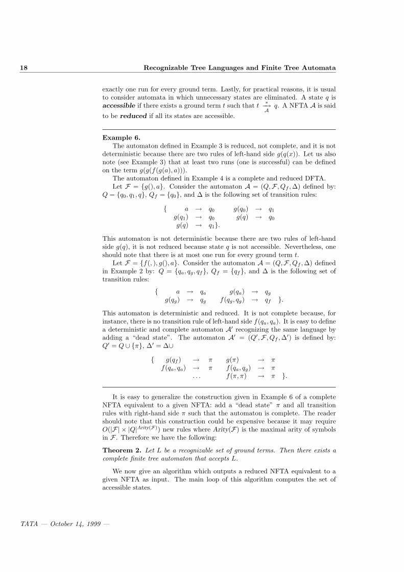
exactly one run for every ground term. Lastly, for practical reasons, it is usualto consider automata in which unnecessary states are eliminated. A state q isaccessible if there exists a ground term t such that t
∗−→A
q. A NFTA A is said
to be reduced if all its states are accessible.
Example 6.The automaton defined in Example 3 is reduced, not complete, and it is not
deterministic because there are two rules of left-hand side g(q(x)). Let us alsonote (see Example 3) that at least two runs (one is successful) can be definedon the term g(g(f(g(a), a))).
The automaton defined in Example 4 is a complete and reduced DFTA.Let F = g(), a. Consider the automaton A = (Q,F , Qf , ∆) defined by:
Q = q0, q1, q, Qf = q0, and ∆ is the following set of transition rules:
a → q0 g(q0) → q1
g(q1) → q0 g(q) → q0
g(q) → q1.This automaton is not deterministic because there are two rules of left-handside g(q), it is not reduced because state q is not accessible. Nevertheless, oneshould note that there is at most one run for every ground term t.
Let F = f(, ), g(), a. Consider the automaton A = (Q,F , Qf , ∆) definedin Example 2 by: Q = qa, qg, qf, Qf = qf, and ∆ is the following set oftransition rules:
a → qa g(qa) → qg
g(qg) → qg f(qg, qg) → qf .This automaton is deterministic and reduced. It is not complete because, forinstance, there is no transition rule of left-hand side f(qa, qa). It is easy to definea deterministic and complete automaton A′ recognizing the same language byadding a “dead state”. The automaton A′ = (Q′,F , Qf , ∆′) is defined by:Q′ = Q ∪ π, ∆′ = ∆∪
g(qf ) → π g(π) → πf(qa, qa) → π f(qa, qg) → π
. . . f(π, π) → π .
It is easy to generalize the construction given in Example 6 of a completeNFTA equivalent to a given NFTA: add a “dead state” π and all transitionrules with right-hand side π such that the automaton is complete. The readershould note that this construction could be expensive because it may requireO(|F| × |Q|Arity(F)) new rules where Arity(F) is the maximal arity of symbolsin F . Therefore we have the following:
Theorem 2. Let L be a recognizable set of ground terms. Then there exists acomplete finite tree automaton that accepts L.
We now give an algorithm which outputs a reduced NFTA equivalent to agiven NFTA as input. The main loop of this algorithm computes the set ofaccessible states.
TATA — October 14, 1999 —

1.1 Finite Tree Automata 19
Reduction Algorithm REDinput: NFTA A = (Q,F , Qf , ∆)begin
Set Marked to ∅ /* Marked is the set of accessible states */repeat
Set Marked to Marked ∪ qwhere
f ∈ Fn, q1, . . . , qn ∈ Marked , f(q1, . . . , qn) → q ∈ ∆until no state can be added to MarkedSet Qr to MarkedSet Qrf
to Qf ∩MarkedSet ∆r to f(q1, . . . , qn) → q ∈ ∆ | q, q1, . . . , qn ∈ Markedoutput: DFTA Ar = (Qr,F , Qrf
, ∆r)end
Obviously all states in the set Marked are accessible, and an easy inductionshows that all accessible states are in the set Marked . And, the NFTA Ar
accepts the tree language L(A). Consequently we have:
Theorem 3. Let L be a recognizable set of ground terms. Then there exists areduced finite tree automaton that accepts L.
Now, we consider the reduction of nondeterminism. Since every DFTA isa NFTA, it is clear that the class of recognizable languages includes the classof languages accepted by DFTA’s. However it turns out that these classes areequal. We prove that, for every NFTA, we can construct an equivalent DFTA.The proof is similar to the proof of equivalence between DFA’s and NFA’s inthe word case. The proof is based on the “subset construction”. Consequently,the number of states of the equivalent DFTA can be exponential in the numberof states of the given NFTA (see Example 8). But, in practice, it often turnsout that many states are not accessible. Therefore, we will present in the proofof the following theorem a construction of a DFTA where only the accessiblestates are considered, i.e. the given algorithm outputs an equivalent and reducedDFTA from a given NFTA as input.
Theorem 4 (The equivalence of DFTA’s and NFTA’s). Let L be a rec-ognizable set of ground terms. Then there exists a DFTA that accepts L.
Proof. First, we give a theoretical construction of a DFTA equivalent to aNFTA. LetA = (Q,F , Qf ,∆) be a NFTA. Define a DFTAAd = (Qd,F , Qdf
,∆d),as follows. The states of Qd are all the subsets of the state set Q of A. That is,Qd = 2Q. We denote by s a state of Qd, i.e. s = q1, . . . , qn for some statesq1, . . . , qn ∈ Q. We define
f(s1, . . . , sn) → s ∈ ∆d
iffs = q ∈ Q | ∃q1 ∈ s1, . . . ,∃qn ∈ sn, f(q1, . . . , qn) → q ∈ ∆.
And Qdfis the set of all states in Qd containing a final state of A.
We now give an algorithmic construction where only the accessible statesare considered.
TATA — October 14, 1999 —

20 Recognizable Tree Languages and Finite Tree Automata
Determinization Algorithm DETinput: NFTA A = (Q,F , Qf , ∆)begin
/* A state s of the equivalent DFTA is in 2Q */Set Qd to ∅; set ∆d to ∅repeat
Set Qd to Qd ∪ s; Set ∆d to ∆d ∪ f(s1, . . . , sn) → swhere
f ∈ Fn, s1, . . . , sn ∈ Qd,s = q ∈ Q | ∃q1 ∈ s1, . . . , qn ∈ sn, f(q1, . . . , qn) → q ∈ ∆
until no rule can be added to ∆Set Qdf
to s ∈ Qd | s ∩Qf 6= ∅output: DFTA Ad = (Qd,F , Qdf
, ∆d)end
It is immediate from the definition of the determinization algorithm thatAd is a deterministic and reduced tree automaton. In order to prove thatL(A) = L(Ad), we now prove that:
(t ∗−−→Ad
s) iff (s = q ∈ Q | t ∗−→A
q).
The proof is an easy induction on the structure of terms.
• base case: let us consider t = a ∈ F0. Then, there is only one rule a → sin ∆d where s = q ∈ Q | a → q ∈ ∆. Consequently, the base case isstraightforward.
• induction step: let us consider a term t = f(t1, . . . , tn). First, let ussuppose that t
∗−−→Ad
f(s1, . . . , sn)→Ads. By induction hypothesis, we
have si = q ∈ Q | ti∗−→A
q, for each i ∈ 1, . . . , n. By construction
of the rule f(s1, . . . , sn) → s ∈ ∆d in the determinization algorithm, it isimmediate that s = q ∈ Q | t
∗−→A
q. Second, if s = q ∈ Q | t∗−→A
q,it is easy to prove that t
∗−−→Ad
s.
Example 7. Let F = f(, ), g(), a. Consider the automatonA = (Q,F , Qf ,∆)defined in Example 3 by: Q = q, qg, qf, Qf = qf, and ∆ =
a → q g(q) → qg(q) → qg g(qg) → qf
f(q, q) → q .
Given A as input, the determinization algorithm outputs the DFTA Ad =(Qd,F , Qdf
,∆d) defined by: Qd = q, q, qg, q, qg, qf, Qdf= q, qg, qf,
TATA — October 14, 1999 —
1.1 Finite Tree Automata 21
and ∆d =
a → qg(q) → q, qg
g(q, qg) → q, qg, qfg(q, qg, qf) → q, qg, qf
∪ f(s1, s2) → q | s1, s2 ∈ Qd .
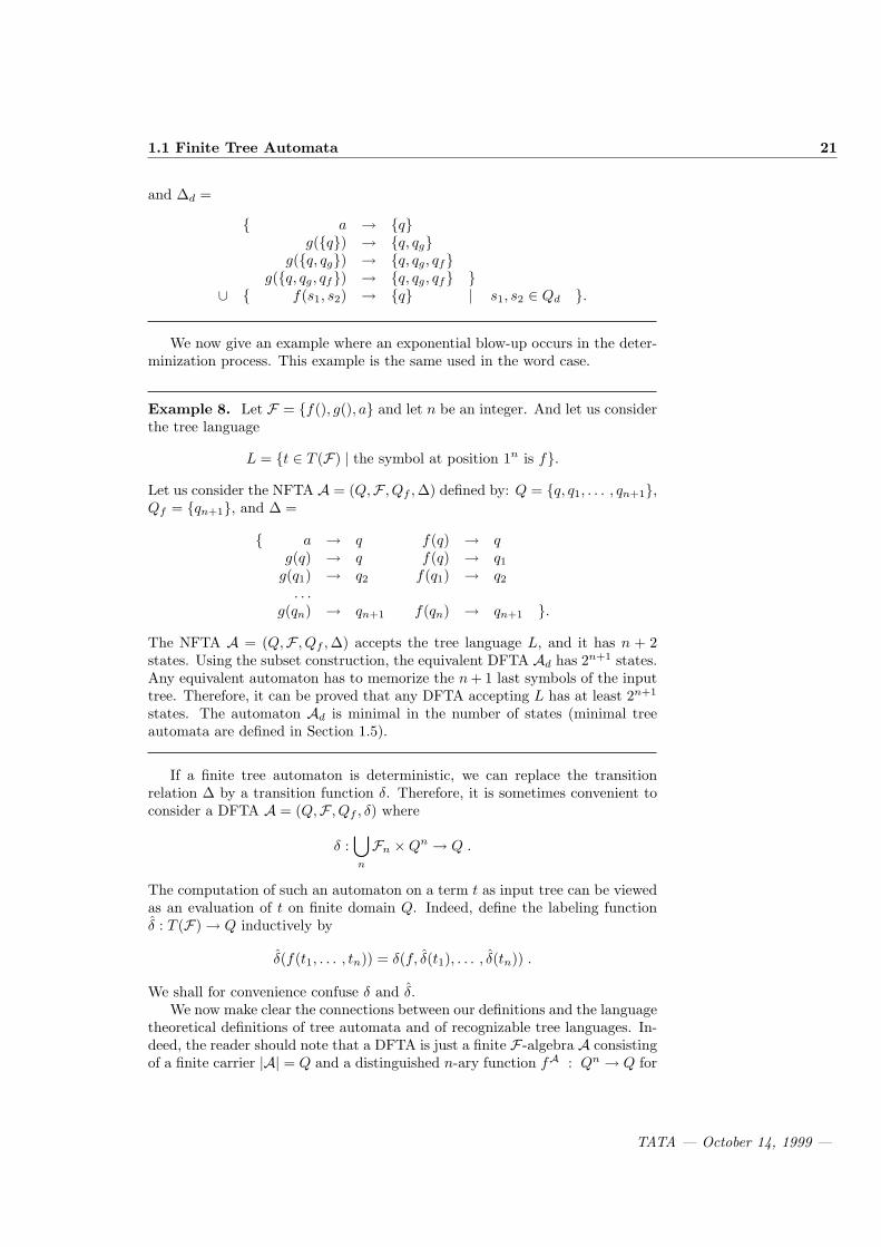
We now give an example where an exponential blow-up occurs in the deter-minization process. This example is the same used in the word case.
Example 8. Let F = f(), g(), a and let n be an integer. And let us considerthe tree language
L = t ∈ T (F) | the symbol at position 1n is f.
Let us consider the NFTA A = (Q,F , Qf , ∆) defined by: Q = q, q1, . . . , qn+1,Qf = qn+1, and ∆ =
a → q f(q) → qg(q) → q f(q) → q1
g(q1) → q2 f(q1) → q2
. . .g(qn) → qn+1 f(qn) → qn+1 .
The NFTA A = (Q,F , Qf , ∆) accepts the tree language L, and it has n + 2states. Using the subset construction, the equivalent DFTA Ad has 2n+1 states.Any equivalent automaton has to memorize the n + 1 last symbols of the inputtree. Therefore, it can be proved that any DFTA accepting L has at least 2n+1
states. The automaton Ad is minimal in the number of states (minimal treeautomata are defined in Section 1.5).
If a finite tree automaton is deterministic, we can replace the transitionrelation ∆ by a transition function δ. Therefore, it is sometimes convenient toconsider a DFTA A = (Q,F , Qf , δ) where
δ :⋃n
Fn ×Qn → Q .
The computation of such an automaton on a term t as input tree can be viewedas an evaluation of t on finite domain Q. Indeed, define the labeling functionδ : T (F) → Q inductively by
δ(f(t1, . . . , tn)) = δ(f, δ(t1), . . . , δ(tn)) .
We shall for convenience confuse δ and δ.We now make clear the connections between our definitions and the language
theoretical definitions of tree automata and of recognizable tree languages. In-deed, the reader should note that a DFTA is just a finite F-algebra A consistingof a finite carrier |A| = Q and a distinguished n-ary function fA : Qn → Q for
TATA — October 14, 1999 —
22 Recognizable Tree Languages and Finite Tree Automata
each n-ary symbol f ∈ F together with a specified subset Qf of Q. A groundterm t is accepted by A if δ(t) = q ∈ Qf where δ is the unique F-algebrahomomorphism δ : T (F) → A.
Example 9. Let F = f(, ), a and consider the F-algebra A with |A| =Q = Z2 = 0, 1, fA = + where the sum is formed modulo 2, aA = 1, and letQf = 0. A and Qf defines a DFTA. The recognized tree language is the setof ground terms over F with an even number of leaves.
Since DFTA and NFTA accept the same sets of tree languages, we shall notdistinguish between them unless it becomes necessary, but shall simply refer toboth as tree automata (FTA).
1.2 The pumping Lemma for Recognizable TreeLanguages
We now give an example of a tree language which is not recognizable.
Example 10. Let F = f(, ), g(), a. Let us consider the tree languageL = f(gi(a), gi(a)) | i > 0. Let us suppose that L is recognizable by anautomaton A having k states. Now, consider the term t = f(gk(a), gk(a)). tbelongs to L, therefore there is a successful run of A on t. As k is the cardinalityof the state set, there are two distinct positions along the first branch of the termlabeled with the same state. Therefore, one could cut the first branch betweenthese two positions leading to a term t′ = f(gj(a), gk(a)) with j < k such thata successful run of A can be defined on t′. This leads to a contradiction withL(A) = L.
This (sketch of) proof can be generalized by proving a pumping lemmafor recognizable tree languages. This lemma is extremely useful in proving thatcertain sets of ground terms are not recognizable. It is also useful for solvingdecision problems like emptiness and finiteness of a recognizable tree language(see Section 1.7).
Pumping Lemma. Let L be a recognizable set of ground terms. Then, thereexists a constant k > 0 satisfying: for every ground term t in L such thatHeight(t) > k, there exist a context C ∈ C(F), a non trivial context C ′ ∈ C(F),and a ground term u such that t = C[C ′[u]] and, for all n ≥ 0 C[C ′
n
[u]] ∈ L.
Proof. Let A = (Q,F , Qf , ∆) be a FTA such that L = L(A) and let k = |Q|be the cardinality of the state set Q. Let us consider a ground term t in Lsuch that Height(t) > k and consider a successful run r of A on t. Now let usconsider a path in t of length strictly greater than k. As k is defined to be thecardinality of the state set Q, there are two positions p1 < p2 along this pathsuch that r(p1) = r(p2) = q for some state q. Let u be the ground subterm of tat position p2. Let u′ be the ground subterm of t at position p1, there exists anon trivial context C ′ such that u′ = C ′[u]. Now define the context C such that
TATA — October 14, 1999 —

1.3 Closure Properties of Recognizable Tree Languages 23
t = C[C ′[u]]. Consider a term C[C ′n
[u]] for some integer n > 1, a successful runcan be defined on this term. Indeed suppose that r corresponds to the reductiont
∗−→A
qf where qf is a final state of A, then we have:
C[C ′n
[u]] ∗−→A
C[C ′n
[q]] ∗−→A
C[C ′n−1
[q]] . . . ∗−→A
C[q] ∗−→A
qf .
The same holds when n = 0.
Example 11. Let F = f(, ), a. Let us consider the tree language L = t ∈T (F) | |Pos(t)| is a prime number. We can prove that L is not recognizable.For all k > 0, consider a term t in L whose height is greater than k. For allcontexts C, non trivial contexts C ′, and terms u such that t = C[C ′[u]], thereexists n such that C[C ′
n
[u]] 6∈ L.
From the Pumping Lemma, it is immediate to derive the following corollary:
Corollary 1. Let A = (Q,F , Qf , ∆) be a FTA. Then L(A) is non empty if andonly there exists a term t in L(A) with Height(t) ≤ |Q|. Then L(A) is infiniteif and only if there exists a term t in L(A) with |Q| < Height(t) ≤ 2× |Q|.
1.3 Closure Properties of Recognizable Tree Lan-guages
A closure property of a class of (tree) languages is the fact that the classis closed under a particular operation. We are interested in effective closureproperties where, given representations for languages in the class, there is analgorithm to construct a representation for the language that results by applyingthe operation to these languages. Let us note that the equivalence betweenNFTA and DFTA is effective, thus we may choose the representation that suitsus best. Nevertheless, the determinization algorithm may output a DFTA whosenumber of states is exponential in the number of states of the given NFTA.For the different closure properties, we give effective constructions and we givethe properties of the resulting FTA depending on the properties of the givenFTA as input. In this section, we consider the Boolean set operations: union,intersection, and complementation. Other operations will be studied in the nextsections. Complexity results are given in Section 1.7.
Theorem 5. The class of recognizable tree languages is closed under union,under complementation, and under intersection.
Union
Let L1 and L2 be two recognizable tree languages. Thus there are tree au-tomata A1 = (Q1,F , Qf1,∆1) and A2 = (Q2,F , Qf2,∆2) with L1 = L(A1)and L2 = L(A2). Since we may rename states of a tree automaton, withoutloss of generality, we may suppose that Q1 ∩ Q2 = ∅. Now, let us considerthe FTA A = (Q,F , Qf , ∆) defined by: Q = Q1 ∪ Q2, Qf = Qf1 ∪ Qf2, and
TATA — October 14, 1999 —

24 Recognizable Tree Languages and Finite Tree Automata
∆ = ∆1∪∆2. The equality between L(A) and L(A1)∪L(A2) is straightforward.Let us note that A is nondeterministic and not complete, even if A1 and A2 aredeterministic and complete.
We now give another construction which preserves determinism. The intu-itive idea is to process in parallel a term by the two automata. For this weconsider a product automaton. Let us suppose that A1 and A2 are complete.And, let us consider the FTA A = (Q,F , Qf ,∆) defined by: Q = Q1 × Q2,Qf = Qf1 ×Q2 ∪Q1 ×Qf2, and ∆ = ∆1 ×∆2 where
∆1 ×∆2 = f((q1, q′1), . . . , f(qn, q′n)) → (q, q′) |
f(q1, . . . , qn) → q ∈ ∆1 f(q′1, . . . , q′n) → q′ ∈ ∆2
It is easy to prove that L(A) = L(A1)∪L(A2). The reader should note that thehypothesis that the two given tree automata are complete is crucial in the proof.Indeed, suppose for instance that a ground term t is accepted by A1 but not byA2. Moreover suppose that A2 is not complete and that there is no run of A2
on t, then the product automaton does not accept t because there is no run ofthe product automaton on t. The reader should also note that the constructionpreserves determinism, i.e. if the two given automata are deterministic, thenthe product automaton is also deterministic.
Complementation
Let L be a recognizable tree language. Let A = (Q,F , Qf , ∆) be a completeDFTA such that L(A) = L. Now, complement the final state set to recognizethe complement of L. That is, let Ac = (Q,F , Qc
f ,∆) with Qcf = Q − Qf ,
the DFTA Ac recognizes the tree language T (F) − L. If you are given with aNFTA, first, it is necessary to apply the determinization algorithm, and secondcomplement the final state set. This could lead to an exponential blow-up.
Intersection
Closure under intersection follows from closure under union and complementa-tion because
L1 ∩ L2 = L1 ∪ L2.
where we denote by L the complement T (F) − L of set L. But if the recog-nizable tree languages are defined by NFTA, we have to use the complemen-tation construction, therefore the determinization process is used leading to anexponential blow-up. Consequently, we now give a direct construction whichdoes not use the determinization algorithm. Let A1 = (Q1,F , Qf1, ∆1) andA2 = (Q2,F , Qf2,∆2) be FTA such that L(A1) = L1 and L(A2) = L2. And,consider the FTA A = (Q,F , Qf ,∆) defined by: Q = Q1×Q2, Qf = Qf1×Qf2,and ∆ = ∆1×∆2. A recognizes L1 ∩L2. Moreover the reader should note thatA is deterministic if A1 and A2 are deterministic.
1.4 Tree homomorphisms
We now consider tree transformations and study the closure properties underthese tree transformations. In this section we are interested with tree transfor-
TATA — October 14, 1999 —

1.4 Tree homomorphisms 25
mations preserving the structure of trees. Thus, we restrict ourselves to treehomomorphisms. Tree homomorphisms are a generalization of homomorphismsfor words (considered as unary terms) to the case of arbitrary ranked alpha-bets. In the word case, it is known that the class of regular sets is closed underhomomorphisms and inverse homomorphisms. The situation is different in thetree case because if recognizable tree languages are closed under inverse ho-momorphisms, they are closed only under a subclass of homomorphisms, i.e.linear homomorphisms (duplication of terms is forbidden). First, we define treehomomorphisms.
Let F and F ′ be two sets of function symbols, possibly not disjoint. Foreach n > 0 such that F contains a symbol of arity n, we define a set of variablesXn = x1, . . . , xn disjoint from F and F ′.
Let hF be a mapping which, with f ∈ F of arity n, associates a termtf ∈ T (F ′,Xn). The tree homomorphism h : T (F) → T (F ′) determined byhF is defined as follows:
• h(a) = ta ∈ T (F ′) for each a ∈ F of arity 0,
• h(f(t1, . . . , tn)) = tfx1 ← h(t1), . . . , xn ← h(tn)where tfx1 ← h(t1), . . . , xn ← h(tn) is the result of applying the substi-
tution x1 ← h(t1), . . . , xn ← h(tn) to the term tf .
Example 12. Let F = g(, , ), a, b and F ′ = f(, ), a, b. Let us consider thetree homomorphism h determined by hF defined by: hF (g) = f(x1, f(x2, x3)),hF (a) = a and hF (b) = b. For instance, we have:
If t =a
b b b
g a
g
, then h(t) =a
b
b b
f
f a
f
f
This homomorphism can be used to transform ternary trees into binary trees.Let us now consider F = and(, ), or(, ), not(), 0, 1 and F ′ = or(, ), not(), 0, 1.Let us consider the tree homomorphism h determined by hF defined by: hF (and) =not(or(not(x1), not(x2)), and hF is the identity otherwise. This homomorphismtransforms a boolean formula in an equivalent boolean formula which does notcontain and.
A tree homomorphism is linear if for each f ∈ F of arity n, hF (f) = tf isa linear term in T (F ′,Xn). The following example shows that tree homomor-phisms do not always preserve recognizability.
Example 13. Let F = f(), g(), a and F ′ = f ′(, ), g(), a. Let us considerthe tree homomorphism h determined by hF defined by: hF (f) = f ′(x1, x1),hF (g) = g(x1), and hF (a) = a. h is not linear. Let L = f(gi(a)) | i ≥ 0,
TATA — October 14, 1999 —

26 Recognizable Tree Languages and Finite Tree Automata
then L is a recognizable tree language. h(L) = f ′(gi(a), gi(a)) | i ≥ 0 is notrecognizable (see Example 10).
Theorem 6 (Linear homomorphisms preserve recognizability). Let h bea linear tree homomorphism and L be a recognizable tree language, then h(L) isa recognizable tree language.
Proof. Let L be a recognizable tree language. Let A = (Q,F , Qf ,∆) be areduced DFTA such that L(A) = L. Let h be a linear tree homomorphism fromT (F) into T (F ′) determined by a mapping hF .
First, let us define a NFTA A′ = (Q′,F ′, Q′f , ∆′). Let us consider a rule r =
f(q1, . . . , qn) → q in ∆ and consider the linear term tf = hF (f) ∈ T (F ′,Xn) andthe set of positions Pos(tf ). We define a set of states Qr = qr
p | p ∈ Pos(tf ),and we define a set of rules ∆r as follows: for all positions p in Pos(tf )
• if tf (p) = g ∈ F ′k, then g(qrp1, . . . , qr
pk) → qrp ∈ ∆r,
• if tf (p) = xi, then qi → qrp ∈ ∆r,
• qrε → q ∈ ∆r.
The preceding construction is made for each rule in ∆. We suppose that all thestate sets Qr are disjoint and that they are disjoint from Q. Now define A′ by:
• Q′ = Q ∪⋃r∈∆ Qr,
• Q′f = Qf ,
• ∆′ =⋃
r∈∆ ∆r.
Second, we have to prove that h(L) = L(A′).
h(L) ⊆ L(A′). We prove that if t∗−→A
q then h(t) ∗−−→A′
q by induction on the
length of the reduction of ground term t ∈ T (F) by automaton A.
• Base case. Suppose that t→A q. Then t = a ∈ F0 and a → q ∈ ∆.Then, by definition of A′, it is easy to prove that h(a) = ta
∗−−→A′
q.
• Induction step.Suppose that t = f(u1, . . . , un), then h(t) = tfx1← h(u1), . . . , xn←h(un). Moreover suppose that t
∗−→A
f(q1, . . . , qn)→A q. By in-
duction hypothesis, we have h(ui)∗−−→A′
qi, for each i in 1, . . . , n.Now by definition of A′, it is easy to prove that tfx1←q1, . . . , xn←qn ∗−−→
A′q.
h(L) ⊇ L(A′). We prove that if t′ ∗−−→A′
q ∈ Q then t′ = h(t) with t∗−→A
q for
some t ∈ T (F). The proof is by induction on the number of states in Q
occurring along the reduction t′ ∗−−→A′
q ∈ Q.
TATA — October 14, 1999 —

1.4 Tree homomorphisms 27
• Base case. Suppose that t′ ∗−−→A′
q ∈ Q and no state in Q apart from q
occurs in the reduction. Then, because the state sets Qr are disjoint,only rules of some ∆r can be used in the reduction. Thus, t′ is ground,t′ = hF (f) for some symbol f ∈ F , and r = f(q1, . . . , qn) → q.Because the automaton is reduced, there is some ground term t withHead(t) = f such that t′ = h(t) and t
∗−→A
q.
• Induction step. Suppose that
t′ ∗−−→A′
vx′1←q1, . . . , x′m←qm ∗−−→A′
q
where v is a linear term in T (F ′, x′1, . . . , x′m), t′ = vx′1← u′1, . . . , x′m←u′m, u′i
∗−−→A′
qi ∈ Q, and no state in Q apart from q occurs in the
reduction of vx′1 ← q1, . . . , x′m ← qm in q. The reader shouldnote that different variables can be substituted by the same state.Then, because the state sets Qr are disjoint, only rules of some∆r can be used in the reduction of vx′1← q1, . . . , x′m← qm in q.Thus, there exists some linear term tf such that vx′1← q1, . . . , x′m←qm = tfx1 ← q1, . . . , xn ← qn for some symbol f ∈ Fn andr = f(q1, . . . , qn) → q ∈ ∆. By induction hypothesis, there areterms u1, . . . , um in L such that u′i = h(ui) and ui
∗−→A
qi for each i in
1, . . . ,m. Now consider the term t = f(v1, . . . , vn), where vi = ui
if xi occurs in tf and vi is some term such that vi∗−→A
qi otherwise
(such vi always exist because A is reduced). We have h(t) = tfx1←h(v1), . . . , xn← h(vn), h(t) = vx′1← h(u1), . . . , x′m← h(um), h(t) =t′. Moreover, by definition of the vi and by induction hypothesis, wehave t
∗−→A
q. Note that if qi occurs more than once, you can sub-
stitute qi by any term satisfying the conditions. The proof does notwork for the non linear case because you have to check that differ-ent occurrences of some state qi corresponding to the same variablexj ∈ Var(tf ) can only be substituted by equal terms.
Only linear tree homomorphisms preserve recognizability. But, now we showthat arbitrary inverse homomorphisms preserve recognizability.
Theorem 7 (Inverse homomorphisms preserve recognizability). Let hbe a tree homomorphism and L be a recognizable tree language, then h−1(L)is a recognizable tree language.
Proof. Let h be a tree homomorphism from T (F) into T (F ′) determined by amapping hF . Let A′ = (Q′,F ′, Q′
f , ∆′) be a complete DFTA such that L(A′) =L. We define a DFTA A = (Q,F , Qf ,∆) by Q = Q′, Qf = Q′
f and ∆ is definedby the following:
if tfx1←q1, . . . , xn←qn ∗−−→A′
q then f(q1, . . . , qn) → q ∈ ∆.
It is obvious that ∆ is computable. It is easy to show by induction on thestructure of terms that t
∗−→A
q if and only if h(t) ∗−−→A′
q.
TATA — October 14, 1999 —

28 Recognizable Tree Languages and Finite Tree Automata
It can be proved that the class of recognizable tree languages is the smallestclass of tree languages closed by linear tree homomorphisms and inverse tree ho-momorphisms. Tree homomorphisms do not in general preserve recognizability,therefore let us consider the following problem: given as instance a recognizabletree language L and a tree homomorphism h, is the set h(L) recognizable ? Toour knowledge it is not known whether this problem is decidable. The readershould note that if this problem is decidable, the problem whether the set ofnormal forms of a rewrite system is recognizable is easily shown decidable (seeExercises 6 and 10).
As a conclusion we consider different special types of tree homomorphisms.These homomorphisms will be used in the next sections in order to simplifysome proofs and will be useful in Chapter 6. Let h be a tree homomorphismdetermined by hF . The tree homomorphism h is said to be:
• ε-free if for each symbol f ∈ F , tf is not reduced to a variable.
• symbol to symbol if for each symbol f ∈ F , Height(tf ) = 1. The readershould note that with our definitions a symbol to symbol tree homomor-phism is ε-free. A linear symbol to symbol tree homomorphism changesthe label of the input symbol, possibly erases some subtrees and possiblymodifies order of subtrees.
• complete if for each symbol f ∈ Fn, Var(tf ) = Xn.
• a delabeling if h is a complete, linear, symbol to symbol tree homomor-phism. Such a delabeling only changes the label of the input symbol andpossibly order of subtrees.
• alphabetic if for each symbol f ∈ Fn, tf = g(x1, . . . , xn), where g ∈ F ′n.
As a corollary of Theorem 6, alphabetic tree homomorphisms, delabelings andlinear, symbol to symbol tree homomorphisms preserve recognizability. It iseasy to prove that for these classes of tree homomorphisms, given h and a FTAA such that L(A) = L as instance, a FTA for the recognizable tree languageh(L) can be constructed in linear time. The same holds for h−1(L).
Example 14. Let F = f(, ), g(), a and F ′ = f ′(, ), g′(), a′. Let us considersome tree homomorphisms h determined by different hF .
• hF (f) = x1, hF (g) = f ′(x1, x1), and hF (a) = a′. h is not linear, notε-free, and not complete.
• hF (f) = g′(x1), hF (g) = f ′(x1, x1), and hF (a) = a′. h is a non linearsymbol to symbol tree homomorphism. h is not complete.
• hF (f) = f ′(x2, x1), hF (g) = g′(x1), and hF (a) = a′. h is a delabeling.
• hF (f) = f ′(x1, x2), hF (g) = g′(x1), and hF (a) = a′. h is an alphabetictree homomorphism.
TATA — October 14, 1999 —

1.5 Minimizing Tree Automata 29
1.5 Minimizing Tree Automata
In this section, we prove that, like in the word case, there exists a unique minimalautomaton in the number of states for a given recognizable tree language.
A Myhill-Nerode Theorem for Tree Languages
The Myhill-Nerode Theorem is a classical result in the theory of finite au-tomata. This theorem gives a characterization of the recognizable sets and ithas numerous applications. A consequence of this theorem, among other con-sequences, is that there is essentially a unique minimum state DFA for everyrecognizable language over finite alphabet. The Myhill-Nerode Theorem gener-alizes in a straightforward way to automata on finite trees.
An equivalence relation ≡ on T (F) is a congruence on T (F) if for everyf ∈ Fn
ui ≡ vi 1 ≤ i ≤ n ⇒ f(u1, . . . , un) ≡ f(v1, . . . , vn) .
It is of finite index if there are only finitely many ≡-classes. Equivalently acongruence is an equivalence relation closed under context, i.e. for all contextsC ∈ C(F), if u ≡ v, then C[u] ≡ C[v]. For a given tree language L, let us definethe congruence ≡L on T (F) by: u ≡L v if for all contexts C ∈ C(F),
C[u] ∈ L iff C[v] ∈ L.
We are now ready to give the Theorem:
Myhill-Nerode Theorem. The following three statements are equivalent:
(i) L is a recognizable tree language
(ii) L is the union of some equivalence classes of a congruence of finite index
(iii) the relation ≡L is a congruence of finite index.
Proof.
• (i) ⇒ (ii) Assume that L is recognized by some complete DFTA A =(Q,F , Qf , δ). We consider δ as a transition function. Let us considerthe relation ≡A defined on T (F) by: u ≡A v if δ(u) = δ(v). Clearly≡A is a congruence relation and it is of finite index, since the number ofequivalence classes is at most the number of states in Q. Furthermore, Lis the union of those equivalence classes that include a term u such thatδ(u) is a final state.
• (ii) ⇒ (iii) Let us denote by ∼ the congruence of finite index. And let usassume that u ∼ v. By an easy induction on the structure of terms, it canbe proved that C[u] ∼ C[v] for all contexts C ∈ C(F). Now, L is the unionof some equivalence classes of ∼, thus we have C[u] ∈ L iff C[v] ∈ L. Thusu ≡L v, and the equivalence class of u in ∼ is contained in the equivalenceclass of u in ≡L. Consequently, the index of ≡L is lower or equal than theindex of ∼ which is finite.
TATA — October 14, 1999 —

30 Recognizable Tree Languages and Finite Tree Automata
• (iii) ⇒ (i) Let Qmin be the finite set of equivalence classes of ≡L. Andlet us denote by [u] the equivalence class of a term u. Let the transitionfunction δmin be defined by:
δmin(f([u1], . . . , [un])) = [f(u1, . . . , un)].
The definition of δmin is consistent because ≡L is a congruence. Andlet Qminf
= [u] | u ∈ L. The DFTA Amin = (Qmin,F , Qminf, δmin)
recognizes the tree language L.
As a corollary of the Myhill-Nerode Theorem, we can deduce an other al-gebraic characterization of recognizable tree languages. This characterizationis a reformulation of the definition of recognizability. A set of ground termsL is recognizable if and only if there exist a finite F-algebra A, a F-algebrahomomorphism φ : T (F) → A and a subset A′ of the carrier |A| of A suchthat L = φ−1(A′).
Minimization of Tree Automata
First, we prove the existence and uniqueness of the minimum DFTA for a rec-ognizable tree language. It is a consequence of the Myhill-Nerode Theorembecause of the following result:
Corollary 2. The minimum DFTA recognizing a recognizable tree language Lis unique up to a renaming of the states and is given by Amin in the proof ofMyhill-Nerode Theorem.
Proof. Assume that L is recognized by some DFTA A = (Q,F , Qf , δ). Therelation ≡A is a refinement of ≡L (see the proof of Myhill-Nerode Theorem).Therefore the number of states of A is greater than or equal to the number ofstates of Amin. If equality holds, A is reduced, i.e. all states are accessible,because otherwise a state could be removed leading to a contradiction. Let qbe a state in Q and let u be such that δ(u) = q. The state q can be identifiedwith the state δmin(u). This identification is consistent and defines a one to onecorrespondence between Q and Qmin.
Second, we give a minimization algorithm for finding the minimum stateDFTA equivalent to a given reduced DFTA. We confuse an equivalence relationand the sequence of its equivalence classes.
Minimization Algorithm MINinput: complete and reduced DFTA A = (Q,F , Qf , δ)begin
Set P to Qf , Q−Qf /* P is the initial equivalence relation*/repeat
P ′ = P/* Refine equivalence P in P ′ */qP ′q′ if
qPq′ and
TATA — October 14, 1999 —

1.6 Top Down Tree Automata 31
∀f ∈ Fn∀q1, . . . , qi−1, qi+1, . . . , qn ∈ Qδ(f(q1, . . . , qi−1, q, qi+1, . . . , qn))Pδ(f(q1, . . . , qi−1, q
′, qi+1, . . . , qn))until P ′ = PSet Qmin to the set of equivalence classes of P/* we denote by [q] the equivalence class of state q w.r.t. P */Set δmin to f([q1], . . . , [qn]) → [f(q1, . . . , qn)]Set Qminf
to [q] | q ∈ Qfoutput: DFTA Amin = (Qmin,F , Qminf
, δmin)end
The DFTA constructed by the algorithmMIN is the minimum state DFTAfor its tree language. Indeed, let A = (Q,F , Qf , ∆) the DFTA to which is ap-plied the algorithm and let L = L(A). Let Amin be the output of the algorithm.It is easy to show that the definition ofAmin is consistent and that L = L(Amin).Now, by contradiction, we can prove that Amin has no more states than thenumber of equivalence classes of ≡L.
1.6 Top Down Tree Automata
Tree automata that we have defined in the previous sections are also known asbottom-up tree automata because these automata start their computation atthe leaves of trees. In this section we define top-down tree automata. Such anautomaton starts its computation at the root in an initial state and then simul-taneously works down the paths of the tree level by level. The tree automatonaccepts a tree if a run built up in this fashion can be defined. It appears thattop-down tree automata and bottom-up tree automata have the same expres-sive power. An important difference between bottom-up tree automata andtop-down automata appears in the question of determinism since deterministictop-down tree automata are strictly less powerful than nondeterministic onesand therefore are strictly less powerful that bottom-up tree automata. Intu-itively, it is due to the following: tree properties specified by deterministictop-down tree automata can depend only on path properties. We now makeprecise these remarks and first, let us formally define top-down tree automata.
A nondeterministic top-down finite Tree Automaton (top-down NFTA)over F is a tuple A = (Q,F , I, ∆) where Q is a set of states (states are unarysymbols), I ⊆ Q is a set of initial states, and ∆ is a set of rewrite rules of thefollowing type :
q(f(x1, . . . , xn)) → f(q1(x1), . . . , qn(xn)),
where n ≥ 0, f ∈ Fn, q, q1, . . . , qn ∈ Q, x1, . . . , xn ∈ X .When n = 0, i.e. when the symbol is a constant symbol a, a transition rule
of top-down NFTA is of the form q(a) → a. A top-down automaton starts at theroot and moves downward, associating along a run a state with each subterminductively. We do not define formally define the move relation →A defined by atop-down NFTA because the definition is easily deduced from the correspondingdefinition for bottom-up NFTA. The tree language L(A) recognized by A is theset of all ground terms t for which there is an initial state q in I such that
q(t) ∗−→A
t.
TATA — October 14, 1999 —

32 Recognizable Tree Languages and Finite Tree Automata
The expressive power of bottom-up and top-down tree automata is the same.Indeed, we have the following Theorem:
Theorem 8 (The equivalence of top-down and bottom-up NFTA’s). Theclass of languages accepted by top-down NFTA’s is exactly the class of recogniz-able tree languages.
Proof. The proof is left to the reader. Hint. Reverse the arrows and exchangethe sets of initial and final states.
Top-down and bottom-up tree automata have the same expressive powerbecause they define the same classes of tree languages. Nevertheless they donot have the same behavior from an algorithmic point of view because nonde-terminism can not be reduced in the class of top-down tree automata.
Proposition 1 (Top-down NFTA’s and top-down DFTA’s). A top-downfinite Tree Automaton (Q,F , I, ∆) is deterministic (top-down DFTA) if thereis one initial state and no two rules with the same left-hand side. Top-downDFTA’s are strictly less powerful than top-down NFTA’s, i.e. there exists arecognizable tree language which is not accepted by a top-down DFTA.
Proof. Let F = f(, ), a, b. And let us consider the recognizable tree languageT = f(a, b), f(b, a). Now let us suppose there exists a top-down DFTA thataccepts T , the automaton should accept the term f(a, a) leading to a contra-diction.
1.7 Decision problems and their complexity
In this section, we study some decision problems and their complexity. The sizeof an automaton will be the size of its representation. More formally:
Definition 1. Let A = (Q,F , Qf , ∆) be an NFTA over F . The size of a rulef(q1(x1), . . . , qn(xn)) → q(f(x1, . . . , xn)) is arity(f) + 1. The size of A noted‖A‖, is defined by:
‖A‖ = |Q|+∑
f(q1(x1),... ,qn(xn))→q(f(x1,... ,xn))∈∆
(arity(f) + 2).
We will work in the frame of RAM machines, with uniform measure.
Membership
Instance A tree automaton and a ground term.
Answer “yes” if and only if the term is recognized by the automaton.
Clearly, the recognizable tree languages are recursive as a NFTA can beviewed as an acceptance algorithm.
Theorem 9. Membership can be decided in linear time for DFTA, in polyno-mial time for NFTA.
Proof. In the deterministic case, an algorithm for testing membership in O(‖t‖+‖A‖) is easy to obtain. For the nondeterministic case, the idea is similar as in theword case: the algorithm determinizes along the computation. The complexityof the algorithm will be in O(‖t‖ × ‖A‖).
TATA — October 14, 1999 —

1.7 Decision problems and their complexity 33
Emptiness
Instance A tree automaton
Answer “yes” if and only if the recognized language is empty.
Theorem 10. It can be decided in linear time whether the language acceptedby a finite tree automaton is empty.
Proof. The minimal height of accepted terms can be bounded by the numberof states using Corollary 1; so, as membership is decidable, emptiness is decid-able. Of course, this approach does not provide a practicable algorithm. Toget an efficient algorithm, it suffices to notice that a NFTA accepts at leastone tree if and only if there is an accessible final state: this algorithm can beviewed as a least fix-point computation.In other words, the language recognizedby a reduced automaton is empty if and only if the set of final states is nonempty. Reducing an automaton can be done in O(|Q| × ‖A‖) by the reductionalgorithm given in Section 1.1. Actually, this algorithm can be improved bychoosing an adequate data structure in order to get a linear algorithm (see Ex-ercise 16). This linear least fixpoint computation holds in serveral frameworks.For example, it can be viewed as the satisfiability test of a set of propositionalHorn formulae. The reduction is easy and linear: each state q can be associatedwith a propositional variable Xq and each rule r : f(q1, . . . , qn) → q can beassociated with a propositional Horn formula Fr = Xq ∨ ¬Xq1 ∨ · · · ∨ ¬Xqn . Itis straightforward that satisfiability of Fr ∪ ¬Xq/q ∈ Qf is equivalent toemptiness of the language recognized by (Q,F , Qf , ∆). So, as satisfiability of aset of propositional Horn formulae can be decided in linear time, we get a linearalgorithm for testing emptiness for NFTA.
The emptiness problem is P-complete with respect to logspace reductions,even when restricted to deterministic tree automata. The proof can easily bedone since the problem is very close to the solvable path systems problem whichis known to be P-complete (see Exercise 17).
Intersection non-emptiness
Instance A finite sequence of tree automata.
Answer “yes” if and only if there is at least one term recognized by eachautomaton of the sequence.
Theorem 11. The intersection problem for tree automata is EXPTIME-complete.
Proof. By constructing the product automata for the n automata, and thentesting non-emptiness, we get an algorithm in O(‖A1‖×· · ·×‖An‖). The proofof EXPTIME-hardness is based on simulation of an alternating linear space-bounded Turing machine. Roughly speaking, with such a machine and an inputof length n can be associated polynomially n tree automata whose intersectioncorresponds to the set of accepting computations on the input. It is worthnoting that the result holds for deterministic top down tree automata as well asfor deterministic bottom-up ones.
TATA — October 14, 1999 —

34 Recognizable Tree Languages and Finite Tree Automata
Finiteness
Instance A tree automaton
Answer “yes” if and only if the recognized language is finite.
Theorem 12. Finiteness can be decided in polynomial time.
Proof. Let us consider a NFTA A = (Q,F , Qf , ∆). Deciding finiteness of A isdirect by Corollary 1: it suffices to find an accepted term t s.t. |Q| < ‖t‖ ≤2∗ |Q|. A more efficient way to test finiteness is to check the existence of a loop:the language is infinite if and only if there is a loop on some useful state, i.e.there exist an accessible state q and contexts C and C ′ such that C[q] ∗−→
Aq
and C ′[q] ∗−→A
q′ for some final state q′. For a given q, deciding if there is a loop
on q can be done in linear time. So, finiteness can be decided in quadratic time,more precisely in O(|Q| × ‖A‖).
Emptiness of the complement
Instance A tree automaton.
Answer “yes” if and only if every term is accepted by the automaton
Deciding whether a deterministic tree automaton recognizes the set of allterms is polynomial for a fixed alphabet: we just have to check whether theautomaton is complete (which can be done in O(|F| × |Q|Arity(F))) and then itremains only to check that all accessible states are final. For nondeterministicautomata, the following result proves in some sense that determinization withits exponential cost is unavoidable:
Theorem 13 (Seidl [Sei90]). The problem whether a tree automaton acceptsthe set of all terms is EXPTIME-complete for nondeterministic tree automata.
Proof. The proof of this theorem is once more based on simulation of linear spacebounded alternating Turing machine: indeed, the complement of the acceptingcomputations on an input w can be coded polynomially in a recognizable treelanguage.
Equivalence
Instance Two tree automata
Answer “yes” if and only if the automata recognize the same language.
Theorem 14. Equivalence is decidable for tree automata.
Proof. Clearly, as the class of recognizable sets is effectively closed under com-plementation and intersection, and as emptiness is decidable, equivalence isdecidable. For two deterministic complete automata A1 and A2, we get bythese means an algorithm in O(‖A1‖ × ‖A2‖). (An other way is to comparethe minimal automata). For nondeterministic ones, this approach leads to anexponential algorithm.
TATA — October 14, 1999 —

1.8 Exercises 35
As we have proved that deciding whether an automaton recognizes the setof all ground terms is EXPTIME-hard, we get immediately:
Corollary 3. The inclusion problem and the equivalence problem for NFTA’sare EXPTIME-complete.
1.8 Exercises
Exercise 1. Let F = f(, ), g(), a. Define a top-down NFTA, a NFTA and a DFTA
for the set G(t) of ground instances of term t = f(f(a, x), g(y)). Is it possible to define
a top-down DFTA for this language?
Exercise 2. Let F = f(, ), g(), a. Define a top-down NFTA, a NFTA and a DFTA
for the set of terms which have a ground instance of term t = f(a, g(y)) as a subterm.
Is it possible to define a top-down DFTA for this language?
Exercise 3. Let F = g(), a. Is the set of ground terms whose height is even
recognizable? Let F = f(, ), g(), a. Is the set of ground terms whose height is even
recognizable?
Exercise 4. Let F = f(, ), a. Prove that the set L = f(t, t) | t ∈ T (F) is
not recognizable. Let F be any ranked alphabet which contains at least one constant
symbol a and one binary symbol f(, ). Prove that the set L = f(t, t) | t ∈ T (F) is
not recognizable.
Exercise 5. Prove the equivalence between top-down NFTA and NFTA.
Exercise 6. Let F = f(, ), g(), a and F ′ = f ′(, ), g(), a. Let us consider thetree homomorphism h determined by hF defined by: hF (f) = f ′(x1, x2), hF (g) =f ′(x1, x1), and hF (a) = a. Is h(T (F)) recognizable? Let L1 = gi(a) | i ≥ 0, thenL1 is a recognizable tree language, is h(L1) recognizable? Let L2 be the recognizabletree language defined by L2 = L(A) where A = (Q,F , Qf , ∆) is defined by: Q =qa, qg, qf, Qf = qf, and ∆ is the following set of transition rules:
a → qa g(qa) → qg
f(qa, qa) → qf f(qg, qg) → qf
f(qa, qg) → qf f(qg, qa) → qf
f(qa, qf ) → qf f(qf , qa) → qf
f(qg, qf ) → qf f(qf , qg) → qf
f(qf , qf ) → qf .
Is h(L2) recognizable?
Exercise 7. Let F1 = or(, ), and(, ), not(), 0, 1, x. A ground term over F can be
viewed as a boolean formula over variable x. Define a DFTA which recognizes the set
of satisfiable boolean formulae over x. Let Fn = or(, ), and(, ), not(), 0, 1, x1, . . . , xn.A ground term over F can be viewed as a boolean formula over variables x1, . . . , xn.
Define a DFTA which recognizes the set of satisfiable boolean formulae over x1, . . . , xn.
Exercise 8. Let t be a linear term in T (F ,X ). Prove that the set G(t) of ground
instances of term t is recognizable. Let R be a finite set of linear terms in T (F ,X ).
Prove that the set G(R) of ground instances of set R is recognizable.
TATA — October 14, 1999 —

36 Recognizable Tree Languages and Finite Tree Automata
Exercise 9. Let R be a finite set of linear terms in T (F ,X ). We define the set
Red(R) of reducible terms for R to be the set of ground terms which have a ground
instance of some term in R as a subterm. Prove that the set Red(R) is recognizable.
Exercise 10. We consider the following two problems. First, given as instance a rec-
ognizable tree language L and a tree homomorphism h, is the set h(L) recognizable?
Second, given as instance a set R of terms in T (F ,X ), is the set Red(R) recogniz-
able? Prove that if the first problem is decidable, the second problem is easily shown
decidable.
Exercise 11. Let R be a finite set of linear terms in T (F ,X ). A term t is inductively
reducible for R if all the ground instances of term t are reducible for R. Prove that
inductive reducibility of a linear term t for a set of linear terms R is decidable.
Exercise 12. Let F = f(, ), a, b.1. Let us consider the set of ground terms L1 defined by the following two condi-
tions:
• f(a, b) ∈ L1,
• t ∈ L1 ⇒ f(a, f(t, b)) ∈ L1.
Prove that the set L1 is recognizable.
2. Prove that the set L2 = t ∈ T (F) | |t|a = |t|b is not recognizable where |t|a(respectively |t|b) denotes the number of a (respectively the number of b) in t.
3. Let L be a recognizable tree language over F . Let us suppose that f is acommutative symbol. Let C(L) be the congruence closure of set L for the setof equations C = f(x, y) = f(y, x). Prove that C(L) is recognizable.
4. Let L be a recognizable tree language over F . Let us suppose that f is a com-mutative and associative symbol. Let AC(L) be the congruence closure of set Lfor the set of equations AC = f(x, y) = f(y, x); f(x, f(y, z)) = f(f(x, y), z).Prove that in general AC(L) is not recognizable.
5. Let L be a recognizable tree language over F . Let us suppose that f is anassociative symbol. Let A(L) be the congruence closure of set L for the set ofequations A = f(x, f(y, z)) = f(f(x, y), z). Prove that in general A(L) is notrecognizable.
Exercise 13. Consider the complement problem:
• Instance A term t ∈ T (F ,X ) and terms t1, . . . , tn,
• Question There is a ground instance of t which is not an instance of any ti.
Prove that the complement problem is decidable whenever term t and all terms ti are
linear. Extend the proof to handle the case where t is a term (not necessarily linear).
Exercise 14. Let F be a ranked alphabet and suppose that F contains some symbolswhich are commutative and associative. The set of ground AC-instances of a term t isthe AC-congruence closure of set G(t). Prove that the set of ground AC-instances of alinear term is recognizable. The reader should note that the set of ground AC-instancesof a set of linear terms is not recognizable (see Exercice refexocloturecetacderec).
Prove that the AC-complement problem is decidable where the AC-complementproblem is defined by:
• Instance A linear term t ∈ T (F ,X ) and linear terms t1, . . . , tn,
• Question There is a ground AC-instance of t which is not an AC-instance ofany ti.
TATA — October 14, 1999 —

1.8 Exercises 37
Exercise 15. Let F be a ranked alphabet and X be a countable set of variables. LetS be a rewrite system on T (F ,X ) (the reader is referred to [DJ90]) and L be a set ofground terms. We denote by S∗(L) the set of reductions of terms in L by S and byS(L) the set of ground S-normal forms of set L. Formally,
S∗(L) = t ∈ T (F) | ∃u ∈ L u∗→ t,
S(L) = t ∈ T (F) | t ∈ IRR(S) and ∃u ∈ L u∗→ t = IRR(S) ∩ S∗(L).
We consider the two following decision problems:
(1rst order reachability)
• Instance A rewrite system S, two ground terms u and v,
• Question v ∈ S∗(u).(2nd order reachability)
• Instance A rewrite system S, two recognizable tree languages L and L′,
• Question S∗(L) ⊆ L′.
1. Let us suppose that rewrite system S satisfies:
(PreservRec) If L is recognizable, then S∗(L) is recognizable.
What can be said about the two reachability decision problems? Give a suffi-cient condition on rewrite system S satisfying (PreservRec) such that S satisfies(NormalFormRec) where (NormalFormRec) is defined by:
(NormalFormRec) If L is recognizable, then S(L) is recognizable.
2. Let F = f(, ), g(), h(), a. Let L = f(t1, t2) | t1, t2 ∈ T (g(), h(), a, and Sis the following set of rewrite rules:
f(g(x), h(y)) → f(x, y) f(h(x), g(y)) → f(x, y)g(h(x)) → x h(g(x)) → xf(a, x) → x f(x, a) → x
Are the sets L, S∗(L), and S(L) recognizable?
3. Let F = f(, ), g(), h(), a. Let L = g(hn(a)) | n ≥ 0, and S is the followingset of rewrite rules:
g(x) → f(x, x) Are the sets L, S∗(L), and S(L) recognizable?
4. Let us suppose now that rewrite system S is linear and monadic, i.e. all rewriterules are of one of the following three types:
(1) l → a , a ∈ F0
(2) l → x , x ∈ Var(l)(3) l → f(x1, . . . , xp) , x1, . . . , xp ∈ Var(l), f ∈ Fp
where l is a linear term (no variable occurs more than once in t) whose heightis greater than 1. Prove that a linear and monadic rewrite system satisfies(PreservRec). Prove that (PreservRec) is false if the right-hand side of rules oftype (3) may be non linear.
Exercise 16. Design a linear-time algorithm for testing emptiness of the languagerecognized by a tree automaton:
Instance A tree automaton
TATA — October 14, 1999 —

38 Recognizable Tree Languages and Finite Tree Automata
Answer “yes” if and only if the language recognized is empty.
Hint: Choose a suitable data structure for the automaton. For example, a state
could be associated with the list of the ”adresses” of the rules whose left-hand side
contain it (eventually, a rule can be repeated); each rule could be just represented by
a counter initialized at the arity of the corresponding symbol and by the state of the
right-hand side. Activating a state will decrement the counters of the corresponding
rules. When the counter of a rule becomes null, the rule can be applied: the right-hand
side state can be activated.
Exercise 17.The Solvable Path Problem is the following:
Instance a finite set X and three sets R ⊂ X ×X ×X, Xs ⊂ X and Xt ⊂ X.
Answer “yes” if and only if Xt ∩A is non empty, where A is the least subset A of Xsuch that Xs ⊂ A and if y, z ∈ A and (x, y, z) ∈ R, then x ∈ A.
Prove that this P − complete problem is log-space reducible to the emptinessproblem for tree automata.
Exercise 18. A flat automaton is a tree automaton which has the following property:there is an ordering ≥ on the states and a particular state q> such that the transitionrules have one of the following forms:
1. f(q>, . . . , q>) → q>
2. f(q1, . . . , qn) → q with q > qi for every i
3. f(q>, . . . , q>, q, q>, . . . , q>) → q
Moreover, we assume that all terms are accepted in the state q>. (The automaton iscalled flat because there are no “nested loop”).
Prove that the intersection of two flat automata is a finite union of automata whosesize is linear in the sum of the original automata. (This contrasts with the constructionof Theorem 5 in which the intersection automaton’s size is the product of the sizes ofits components).
Deduce from the above result that the intersection non-emptiness problem for flat
automata is in NP (compare with Theorem 11).
1.9 Bibliographic Notes
Tree automata were introduced by Doner [Don65, Don70] and Thatcher andWright [TW65, TW68]. Their goal was to prove the decidability of the weaksecond order theory of multiple successors. The original definitions are basedon the algebraic approach and involve heavy use of universal algebra and/orcategory theory.
Many of the basic results presented in this chapter are the straightforwardgeneralization of the corresponding results for finite automata. It is difficult toattribute a particular result to any one paper. Thus, we only give a list of someimportant contributions consisting of the above mentioned papers of Doner,Thatcher and Wright and also Eilenberg and Wright [EW67], Thatcher [Tha70],Brainerd [Bra68, Bra69], Arbib and Give’on [AG68]. All the results of thischapter and a more complete and detailed list of references can be found in thetextbook of Gecseg and Steinby [GS84] and also in their recent survey [GS96].For an overview of the notion of recognizability in general algebraic structuressee Courcelle [Cou89] and the fundamental paper of Mezei and Wright [MW67].
TATA — October 14, 1999 —
1.9 Bibliographic Notes 39
In Nivat and Podelski [NP89] and [Pod92], the theory of recognizable tree lan-guages is reduced to the theory of recognizable sets in an infinitely generatedfree monoid.
The results of Sections 1.1, 1.2, and 1.3 were noted in many of the papersmentioned above, but, in this textbook, we present these results in the style ofthe undergraduate textbook on finite automata by Hopcroft and Ullman [HU79].Tree homomorphisms were defined as a special case of tree transducers, seeThatcher [Tha73]. The reader is referred to the bibliographic notes in Chapter 6of the present textbook for detailed references. The reader should note that ourproof of preservation of recognizability by tree homomorphisms and inverse treehomomorphisms is a direct construction using FTA. A more classical proof canbe found in [GS84] and uses regular tree grammars (see Chapter 2).
Minimal tree recognizers and Nerode’s congruence appear in Brainerd [Bra68,Bra69], Arbib and Give’on [AG68], and Eilenberg and Wright [EW67]. Theproof we presented here is by Kozen [Koz92] (see also Fulop and Vagvolgyi [FV89]).Top-down tree automata were first defined by Rabin [Rab69]. The reader isreferred to [GS84] and [GS96] for more references and for the study of somesubclasses of recognizable tree languages such as the tree languages recognizedby deterministic top-down tree automata.
Some results of Sections 1.7 are “folklore” results. Many interesting resultsconcerning complexity and tree automata can be found in Seidl [Sei89], [Sei90].The EXPTIME-hardness of the problem of intersection non-emptiness is oftenused; this problem is close to problems of type inference and an idea of the proofcan be found in [FSVY91]. A proof for deterministic top-down automata canbe found in [Sei94b]. A detailed proof in the deterministic bottom-up case aswell as some other results about complexity and tree automata can be foundin [Vea97a], [Vea97b].
Recently, applications of tree automata theory to automated deduction andto the theory of rewriting systems were studied. Numerous exercises of thepresent section introduce these applications. These applications are studied inmore details in Section 3.4. Most of the recent results about tree automata andrewrite systems are collected in Gilleron and Tison [GT95]. Let S be a termrewrite system (see for example Dershowitz and Jouannaud [DJ90] for a surveyon rewrite systems), if S is left-linear the set IRR(S) of irreducible ground termsw.r.t. S is a recognizable tree language. This result first appears in Gallier andBook [GB85] and is the subject of Exercise 9. However not every recognizabletree language is the set of irreducible terms w.r.t. a rewrite system S (seeFulop and Vagvolgyi [FV88]). It was proved that the problem whether, givena rewrite system S as instance, the set of irreducible terms is recognizable isdecidable (Kucherov [Kuc91]). The problem of preservation of regularity by treehomomorphisms is not known decidable. Exercise 10 shows that this problemis stronger than the previous one.
The notion of inductive reducibility (or ground reducibility) was introducedin automated deduction. A term t is S-inductively (or S-ground) reducible forS if all the ground instances of term t are reducible for S. Inductive reducibilityis decidable for linear term t and left-linear rewrite system S. This is Exer-cise 11, see also Section 3.4.2. Inductive reducibility is decidable for finite S(see Plaisted [Pla85]). Complement problems are also introduced in automateddeduction. They are the subject of Exercises 13 and 14. The complement prob-lem for linear terms was proved decidable by Lassez and Marriott [LM87] and
TATA — October 14, 1999 —

40 Recognizable Tree Languages and Finite Tree Automata
the AC-complement problem by Lugiez and Moysset [LM94].The reachability problem is defined in Exercise 15. It is well known that this
problem is undecidable in general. It is decidable for rewrite systems preservingrecognizability, i.e. such that for every recognizable tree language L, the setof reductions of terms in L by S is recognizable. This is true for linear andmonadic rewrite systems (right-hand sides have depth less than 1). This resultwas obtained by K. Salomaa [Sal88] and is the matter of Exercise 15. This istrue also for linear and semi-monadic (variables in the right-hand sides havedepth at most 1) rewrite systems, Coquide et al. [CDGV94]. Other interestingresults can be found in [Jac96].
TATA — October 14, 1999 —

Chapter 2
Regular grammars andregular expressions
2.1 Tree Grammar
In the previous chapter, we have studied regular tree languages from the ac-ceptor point of view, using tree automata. In this chapter we study regularlanguages from the generation point of view, using tree grammars. Again, weshall find that many properties and concepts on word languages smoothly gener-alize to tree languages and that algebraic characterization of regular languagesdo exist for tree languages. Actually, this is not surprising since tree languagescan be seen as word languages on an infinite alphabet of contexts with one hole.We shall show also that the set of derivations of a context-free language is aregular tree language.
2.1.1 Definitions
When we write programs, we often have to know how to produce the elements ofthe data structures that we use. For instance, a definition of the lists of integersin a functional language like ML is similar to the following definition:
Nat = 0 | s(Nat)List = nil | cons(Nat, List)
This definition is nothing but a tree grammar in disguise, more precisely theset of lists of integers is the tree language generated by the grammar with axiomList, non-terminal symbols List,Nat, terminal symbols 0, s, nil, cons and rules
Nat → 0Nat → s(Nat)List → nilList → cons(Nat, List)
Tree grammars are similar to word grammars except that basic objects aretrees, therefore terminals and non-terminals may have an arity greater than 0.More precisely, a tree grammar G = (A,N,F , R) is composed of an axiomA, a set N of non-terminal symbols with A ∈ N , a set F of terminal
TATA — October 14, 1999 —

42 Regular grammars and regular expressions
symbols, a set R of production rules of the form α → β where α, β are treesof T (F∪N∪X ) where X is a set of dummy variables and α contains at least onenon-terminal. Moreover we require that F ∩N = ∅, that each element of N ∪Fhas a fixed arity and that the arity of the axiom A is 0. In this chapter, weshall concentrate on regular tree grammars where a regular tree grammarG = (A,N,F , R) is a tree grammar such that all non-terminal symbols havearity 0 and production rules have the form X → β, with X a non-terminal ofN and β a tree of T (F ∪N).
Example 15. The grammar G with axiom List, non-terminals List,Natterminals 0, nil, s(), cons(, ), rules
List → nilList → cons(Nat, List)Nat → 0Nat → s(Nat)
is a regular tree grammar.
A tree grammar is used to build terms from the axiom, using the corre-sponding derivation relation. Basically the idea is to replace a non-terminalX by the right-hand side α of a rule X → α. More precisely, given a regulartree grammar G = (A,N,F , R), the derivation relation → associated to G isa relation on pairs of terms of T (F ∪ N) such that s → t if and only if thereare a rule X → α ∈ R, a context C such that s = C[X] and t = C[α]. Thelanguage generated by G, denoted by L(G), is the set of terms of T (F)which can be reached by successive derivations starting from the axiom, i.e.L(G) = s ∈ TF | A
+→ s with +→ the transitive closure of →.
Example 16. Let G be the grammar of the previous example, then a derivationof cons(s(0), nil) from List is
List →G cons(Nat, List) →G cons(s(Nat), List) →G cons(s(Nat), nil) →G cons(s(0), nil)
and the language generated by G is the set of lists of non-negative integers.
From the example, we can see that trees are generated top-down by replacinga leaf by some other term. When X is a non-terminal of a regular tree grammarG, we denote by LG(X) the language generated by the grammar G′ identical toG but with X as axiom. When there is no ambiguity on the grammar referred to,we drop the subscript G. We say that two grammars G and G′ are equivalentwhen they generate the same language. Grammars can contain useless rules ornon-terminals and we want to get rid of these while preserving the generatedlanguage. A non-terminal is reachable if there is a derivation from the axiomcontaining this non-terminal. A non-terminal X is productive if LG(X) is non-empty. A regular tree grammar is reduced if and only if all its non-terminalsare reachable and productive. We have the following result:
Proposition 2. A regular tree grammar is equivalent to a normalized regulartree grammar.
TATA — October 14, 1999 —

2.1 Tree Grammar 43
Proof. Given a grammar G = (A,N,F , R), we can compute the set of reachableterminals and the set of productive terminals using the sequences (Reach)n and(Prod)n which are defined in the following way.
Prod0 = ∅Prodn = Prodn−1
∪X ∈ N | ∃(X → α) ∈ R and each non-terminal of α is in Prodn−1
and
Reach0 = AReachn = Reachn−1
∪X ∈ N | ∃(X ′ → α) ∈ R such that X ′ ∈ Reachn−1 and X occurs in α
For each sequence, there is an index such that all elements of the sequencewith greater index are identical and this element is the set of productive (resp.reachable) non-terminals of G. Each regular tree grammar is equivalent to areduced tree grammar which is computed by the following cleaning algorithm.
Computation of an equivalent reduced grammarinput: a regular tree grammar G = (A,N,F , R).
1. Compute the set of productive literals NProd using the sequence (Prod)n
and let G′ = (A,N ′,F , R) where N ′ = N ∩NProd and R′ is the subset ofR involving rules containing only productive non-terminals.
2. Compute the set NReach of reachable terminals NReach using the sequence(Reach)n and let G′′ = (A,N ′ ∩NReach,F , R′′) where R′′ is the subset ofR′ involving rules containing only reachable terminals.
output: G′′
The equivalence of G,G′ and G′′ is straightforward. Moreover each non-terminal X of G′′ must appear in a derivation A
∗→C[X] ∗→C[s] which provesthat G′′ is reduced. The reader should notice that to exchange the two steps ofthe computation may result in a grammar which is not reduced (see Exercise 21).
Actually, we shall use even simpler grammars, i.e. normalized regular treegrammar, where the production rules have the form X → f(X1, . . . , Xn) orX → a where f, a are symbols of F and X, X1, . . . , Xn are non-terminals. Thefollowing result shows that this is not a restriction.
Proposition 3. A regular tree grammar is equivalent to a normalized regulartree grammar.
Proof. Replace a rule X → f(s1, . . . , sn) by X → f(X1, . . . , Xn) with Xi = si
if si ∈ N otherwise Xi is a new non-terminal. In the last case add the ruleXi → si. Iterate this process until one gets a (necessarily equivalent) grammarwith rules of the form X → f(X1, . . . , Xn) or X → a or X1 → X2. Thelast rules are replaced by the rules X1 → α for all α 6∈ N such that X1
+→Xi
and Xi → α ∈ R (these X ′is are easily computed using a transitive closure
algorithm).
TATA — October 14, 1999 —

44 Regular grammars and regular expressions
From now on, we assume that all grammars are normalized, unless this isstated otherwise explicitly.
2.1.2 Regular tree grammar and recognizable tree lan-guages
Given some normalized regular tree grammar G = (A, N,F , RG), we show howto build a top-down tree automaton which recognizes L(G). We define A =(Q,F , I, ∆) by
• Q = qX | X ∈ N• I = qA• qX(f(x1, . . . , xn)) → f(qX1(x1), . . . , qXn
(xn)) ∈ ∆ if and only if X →f(X1, . . . , Xn) ∈ RG.
A standard proof by induction on derivation length yields L(G) = L(A). There-fore we have proved that the languages generated by regular tree grammar arerecognizable languages.
The next question to ask is whether recognizable tree languages can begenerated by regular tree grammars. If L is a regular tree language, thereexists a top-down tree automata A = (Q,F , I, ∆) such that L = L(A). Wedefine G = (A,N,F , RG) with A a new symbol, N = Xq | q ∈ Q, RG =Xq → f(Xq1 , . . . , Xqn) | q(f(x1, . . . , xn)) → f(q1(x1), . . . , qn(xn)) ∈ R ∪A → XI | XI ∈ I. A standard proof by induction on derivation length yieldsL(G) = L(A).
Combining these two properties, we get the equivalence between recognizablelanguages and the languages generated by regular tree grammars.
Theorem 15. A tree language is recognizable if and only if it is generated by aregular tree grammar.
2.2 Regular expressions. Kleene’s theorem fortree languages.
Going back to our example of lists of nonnegative integers, we can write the setsdefined by the non-terminals Nat and List as follows.
Nat = 0, s(0), s(s(0)), . . . List = nil, cons( , nil), cons( , cons( , nil), . . .
where stands for any element of Nat. There is some regularity in each setwhich reminds of the regularity obtained with regular word expressions con-structed with the union, concatenation and iteration operators. Therefore wecan try to use the same idea to denote the sets Nat and List. However, since weare dealing with trees and not words, we must put some information to indicatewhere concatenation and iteration must take place. This is done by using anew symbol which behaves as a constant. Moreover, since we have two indepen-dent iterations, the first one for Nat and the second one for List, we shall usetwo different new symbols 21 and 22 and a natural extension of regular wordexpression leads us to denote the sets Nat and List as follows.
TATA — October 14, 1999 —

2.2 Regular expressions. Kleene’s theorem for tree languages. 45
Nat = s(21)∗,21 .21 0List = nil + cons( (s(21)∗,21 .21 0) , 22)∗,22 .22 nil
We are going to show that this is a general phenomenon and that we can definea notion of regular expressions for trees and that Kleene’s theorem for wordscan be generalized to trees. Like in the example, we must introduce a particularset of constants K which are used to indicate the positions where concatenationand iteration take place in trees. This explains why the syntax of regular treeexpressions is more cumbersome than the syntax of word regular expressions.These new constants are usually denoted by 21, 22, . . . . Therefore, in thissection, we consider trees constructed on F ∪K where K is a distinguished finiteset of symbols of arity 0 disjoint from F .
2.2.1 Substitution and iteration
First, we have to generalize the notion of substitution to languages, replacingsome 2i by a tree of some language Li. The main difference with term sub-stitution is that different occurrences of the same constant 2i can be replacedby different terms of Li. Given a tree t of T (F ∪ K), 21, . . . , 2n symbols of Kand L1, . . . , Ln languages of T (F ∪K), the tree substitution (substitution forshort) of 21, . . . , 2n by L1, . . . , Ln in t, denoted by t21←L1, . . . , 2n←Ln,is the tree language defined by the following identities.
• 2i21←L1, . . . , 2n←Ln = Li for i = 1, . . . , n,
• a21←L1, . . . , 2n←Ln = a for all a ∈ F ∪K such that arity of a is 0and a 6= 21, . . . , a 6= 2n,
• f(s1, . . . , sn)21← L1, . . . , 2n← Ln = f(t1, . . . , tn) | ti ∈ si21← L1, . . . , 2n←Ln
Example 17. Let F = 0, nil, s(), cons(, ) and K = 21,22, let
t = cons(21, cons(21, 22))
and letL1 = 0, s(0)
then
t21←L = cons(0, cons(0, 22)),cons(0, cons(s(0),22)),cons(s(0), cons(0,22)),cons(s(0), cons(s(0), 22))
Symbols of K are mainly used to distinguish places where the substitutionmust take place, and they are usually not relevant. For instance, if t is a treeon the alphabet F ∪ 2 and L be a language of trees on the alphabet F , thenthe trees of t2 ← L don’t contain the symbol 2.
The substitution operation generalizes to languages in a straightforward way.When L,L1, . . . , Ln are languages of T (F∪K) and 21, . . . , 2n are elements ofK,
TATA — October 14, 1999 —

46 Regular grammars and regular expressions
we define L21←L1, . . . , 2n←Ln to be the set⋃
t∈L t21←L1, . . . , 2n←Ln.
Now, we can define the concatenation operation for tree languages. Given Land M two languages of TF∪K, and 2 be a element of K, the concatenationof M to L through 2, denoted by L .2 M , is the set of trees obtained bysubstituting the occurrence of 2 in trees of L by trees of M , i.e. L .2 M =⋃
t∈Lt2←M.To define the closure of a language, we must define the sequence of successive
iterations. Given L a language of T (F∪K) and 2 an element of K, the sequenceLn,2 is defined by the equalities.
• L0, 2 = 2
• Ln+1, 2 = Ln, 2 ∪ Ln, 2 .2 L
The closure L∗,2 of L is the union of all Ln, 2 for nonnegative n, i.e., L∗,2 =∪nLn,2. From the definition, one gets that 2 ⊆ L∗,2 for any L.
Example 18. Let F = 0, nil, s(), cons(, ), let L = 0, cons(0, 2) andM = nil, cons(s(0), 2), then
L .2 M = 0, cons(0, nil), cons(0, cons(s(0), 2))L∗,2 = 2∪
0, cons(0, 2)∪0, cons(0, nil), cons(0, cons(s(0), 2)) ∪ . . .
We prove now that the substitution and concatenation operations yield reg-ular languages when they are applied to regular languages.
Proposition 4. Let L be a regular tree language on F ∪ K, let L1, . . . , Ln beregular tree languages on F ∪K, let 21, . . . , 2n ∈ K, then L21←L1, . . . , 2n←Ln is a regular tree language.
Proof. Since L is regular, there exists some normalized regular tree grammarG = (A,N,F ∪ K, R) such that L = L(G), and for each i = 1, . . . , n thereexists a normalized grammar Gi = (Ai, Ni,F ∪ K, Ri) such that Li = L(Gi).We can assume that the sets of non-terminals are pairwise disjoint. The ideaof the proof is to construct a grammar G′ which starts by generating trees likeG but replaces the generation of a symbol 2i by the generation of a tree ofLi via a branching towards the axiom of Gi. More precisely, we show thatL21←L1, . . . , 2n←Ln = L(G′) where G′ = (A,N ′,F ∪ K, R′) such that
• N ′ = N ∪N1 ∪ . . . ∪Nn,
• R′ contains the rules of Ri and the rules of R but the rules X → 2i whichare replaced by the rules X → Ai, where Ai is the axiom of Li.
TATA — October 14, 1999 —

2.2 Regular expressions. Kleene’s theorem for tree languages. 47
ci ci
X → ci X → ci
Ai+→ s Ai
+→ s′
A straightforward induction on the height of trees proves that G′ generateseach tree of L21←L1, . . . , 2n←Ln.
The converse is to prove that L(G′) ⊆ L21← L1, . . . , 2n← Ln. Thisis achieved by proving the following property by induction on the derivationlength.
X+→ s′ where s′ ∈ T (F ∪ K) using the rules of G′
if and only ifthere is some s such that X
+→ s using the rules of G ands′ ∈ s21←L1, . . . , 2n←Ln.
• base case: X → s in one step. Therefore this derivation is a derivation ofthe grammar G and no 2i occurs in s, yielding s ∈ L21←L1, . . . , 2n←Ln
• induction step: we assume that the property is true for any terminaland derivation of length less than n. Let X be such that X → s′ in n
steps. This derivation can be decomposed as X → s1+→ s′. We distinguish
several cases depending on the rule used in the derivation X → s1.
– the rule is X → f(X1, . . . , Xm), therefore s′ = f(t1, . . . , tm) and ti ∈L(Xi)21← L1, . . . , 2n← Ln, therefore s′ ∈ L(X)21← L1, . . . , 2n←Ln,
– the rule is X → Ai, therefore X → 2i ∈ R and s′ ∈ Li and s′ ∈L(X)21←L1, . . . , 2n←Ln.
– the rule X → a with a ∈ F , a of arity 0, a 6= 21, . . . , a 6= 2n are notconsidered since no further derivation can be done.
The following proposition states that regular languages are stable also underclosure.
TATA — October 14, 1999 —

48 Regular grammars and regular expressions
Proposition 5. Let L be a regular tree language of T (F ∪K), let 2 ∈ K, thenL∗,2 is a regular tree language of T (F ∪ K).
Proof. There exists a normalized regular grammar G = (A,N,F ∪ K, R) suchthat L = L(G) and we obtain from G a grammar G′ = (A′, N ∪A′,F ∪K, R′)for L∗,2 by replacing rules leading to 2 such as X → 2 by rules X → A leadingto the axiom. Moreover we add the rule A′ → 2 to generate 2 = L0,2 andthe rule A′ → A to generate Li,2 for i > 0. By construction G′ generates theelements of L∗,2.
Conversely a proof by induction on the length on the derivation proves thatL(G′) ⊆ L∗,2.
2.2.2 Regular expressions and regular tree languages.
Now, we can define regular tree expression in the flavor of regular word expres-sion using the +, .2,∗,2 operators.
Definition 2. The set Regexp(F ,K) of regular tree expressions on F andK is the smallest set such that:
• the empty set ∅ is in Regexp(F ,K)
• if a ∈ F0 ∪ K is a constant, then a ∈ Regexp(F ,K),
• if f ∈ Fn has arity n > 0 and E1, . . . , En are regular expressions ofRegexp(F ,K) then f(E1, . . . , En) is a regular expression of Regexp(F ,K),
• if E1, E2 are regular expressions of Regexp(F ,K) then (E1 + E2) is aregular expression of Regexp(F ,K),
• if E1, E2 are regular expressions of Regexp(F ,K) and 2 is an element ofK then E1 .2 E2 is a regular expression of Regexp(F ,K),
• if E is a regular expression of Regexp(F ,K) and 2 is an element of Kthen E∗,2 is a regular expression of Regexp(F ,K).
Each regular expression E represents a set of terms of T (F ∪ K) which wedenote [[E]] and which is formally defined by the following equalities.
• [[∅]] = ∅,• [[a]] = a for a ∈ F0 ∪ K,
• [[f(E1, . . . , En)]] = f(s1, . . . , sn) | s1 ∈ [[E1]], . . . , sn ∈ [[En]],• [[E1 + E2]] = [[E1]] ∪ [[E2]],
• [[E1.2 E2]] = [[E1]]2←[[E2]],• [[E∗,2]] = [[E]]∗,2
Example 19. Let F = 0, nil, s(), cons(, ) and 2 ∈ K then
nil + (cons(0, 2)∗,2).2nil
TATA — October 14, 1999 —

2.2 Regular expressions. Kleene’s theorem for tree languages. 49
is a regular expression of Regexp(F ,K) which denotes the set of lists of zeros:
nil, cons(0, nil), cons(0, cons(0, nil)), . . .
In the remaining of this section, we compare the relative expressive powerof regular expressions and regular languages. It is easy to prove that for eachregular expression E, the set [[E]] is a regular tree language. The proof is doneby structural induction on E. The first three cases are obvious and the two lastcases are consequences of Propositions 5 and 4. The converse, i.e. a regular treelanguage can be denoted by a regular expression, is more involved and the proofis similar to the proof of Kleene’s theorem for word language. Let us state theresult first.
Proposition 6. Let A = (Q,F , QF ,∆) be a bottom-up tree automaton, thenthere exists a regular expression E of Regexp(F , Q) such that L(A) = [[E]].
The occurrence of symbols of Q in the regular expression denoting L(A)doesn’t cause any trouble since we have seen that a regular expression of Regexp(F , Q)can denote a language of TF .
Proof. The proof is similar to the proof for word languages and word automata.For each 1 ≤ i, j,≤ |Q|,K ⊆ Q, we define the set T (i, j,K) as the set of trees tof T (F ∪K) such that
• if an element of K appears in t then it is a leaf,
• each leaf of t is in K or no leaf is in K,
• there is a run r of A such that
– r(ε) = qi,
– for each p ∈ Pos(()t) such that p is not a position of leaf nor of theroot, r(p) ∈ q1, . . . , qj.
Roughly speaking, a term is in T (i, j, K) if we can reach qi at the root byusing only states in q1, . . . , qj when we assume that the leaves are statesof K. By definition, L(A) the language accepted by A is the union of theT (i, |Q|, ∅)’s for i such that qi is a final state: these terms are the terms ofT (F) such that there is a successful run using any possible state of Q. Now, weprove by induction on j that T (i, j, K) can be denoted by a regular expressionof Regexp(F , Q).
• Base case j = 0. The set T (i, 0, K) is the set of trees t where the root islabelled by qi, the leaves are in F ∪ K and no internal node is labelledby some q. Therefore there exist a1, . . . , an, a ∈ F ∪ K such that t =f(a1, . . . , an) or t = a, hence T (i, j, ∅) is finite and can be denoted by aregular expression of Regexp(F ∪Q).
• Induction case. Let us assume that for any i′,K ′ ⊆ Q and 0 ≤ j′ < j, theset T (i′, j′,K ′) can be denoted by a regular expression. We can write thefollowing equality:
TATA — October 14, 1999 —
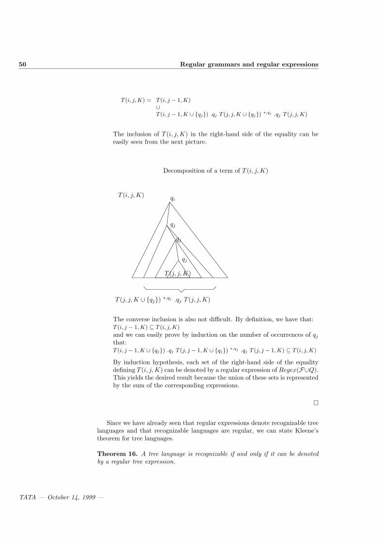
50 Regular grammars and regular expressions
T (i, j, K) = T (i, j − 1, K)∪T (i, j − 1, K ∪ qj) .qj T (j, j, K ∪ qj) ∗,qj .qj T (j, j, K)
The inclusion of T (i, j, K) in the right-hand side of the equality can beeasily seen from the next picture.
Decomposition of a term of T (i, j,K)
T (i, j,K) qi
qj
qj
qj
T (j, j,K)
T (j, j,K ∪ qj) ∗,qj .qj T (j, j, K)
The converse inclusion is also not difficult. By definition, we have that:T (i, j − 1, K) ⊆ T (i, j, K)
and we can easily prove by induction on the number of occurrences of qj
that:T (i, j − 1, K ∪ qj) .qj T (j, j − 1, K ∪ qj) ∗,qj .qj T (j, j − 1, K) ⊆ T (i, j, K)
By induction hypothesis, each set of the right-hand side of the equalitydefining T (i, j, K) can be denoted by a regular expression of Regex(F∪Q).This yields the desired result because the union of these sets is representedby the sum of the corresponding expressions.
Since we have already seen that regular expressions denote recognizable treelanguages and that recognizable languages are regular, we can state Kleene’stheorem for tree languages.
Theorem 16. A tree language is recognizable if and only if it can be denotedby a regular tree expression.
TATA — October 14, 1999 —

2.3 Regular equations. 51
2.3 Regular equations.
Looking at our example of the set of lists of natural numbers, we can realize thatthese lists can be defined by equations instead of grammar rules. For instance,denoting set union by +, we could replace the grammar given in Section 2.1.1by the following equations.
Nat = 0 + s(Nat)List = nil + cons(Nat, List)
where the variables are List and Nat. To get the usual lists of nonnegativenumbers, we must restrict ourselves to the least fixed-point solution of this setof equations. Systems of language equations do not always have solution nordoes a least solution always exist. Therefore we shall study regular equationsystems defined as follows.
Definition 3. Let X1, . . . , Xn be variables denoting sets of trees, let sji be terms
over F∪X1, . . . , Xn for 1 ≤ j ≤ ni, 1 ≤ i ≤ n, then a regular equation systemS is a set of equations of the form:
X1 = s11 + . . . + s1
n1
. . .Xp = sp
1 + . . . + spnp
A solution of S is any n-tuple (L1, . . . , Ln) of languages of TF such that
L1 = s11X1←L1, . . . , Xn←Ln ∪ . . . ∪ s1
n1X1←L1, . . . , Xn←Ln. . .
Lp = sp1X1←L1, . . . , Xn←Ln ∪ . . . ∪ sp
npX1←L1, . . . , Xn←Ln
We define the ordering⊆ on T (F)×. . .×T (F) by (L1, . . . , Ln) ⊆ (L′1, . . . , L′n)if and only if Li ⊆ L′i for all i = 1, . . . , n. From the definition, we have that(∅, . . . , ∅) is the smallest element of ⊆ and that each increasing sequence has anupper bound. The fixed-point operator T S associated with an equation systemS is an operator from (T (F), . . . , T (F)) into (T (F), . . . , T (F)) such that
T S(L1, . . . , Ln) = (L′1, . . . , L′n)whereL′1 = L1 ∪ s1
1X1←L1, . . . , Xn←Ln ∪ . . . ∪ s1n1X1←L1, . . . , Xn←Ln
. . .L′p = Lp ∪ sp
1X1←L1, . . . , Xn←Ln ∪ . . . ∪ spnpX1←L1, . . . , Xn←Ln
Example 20. Let S be
Nat = 0 + s(Nat)List = nil + cons(Nat, List)
then
T S(∅, ∅) = (0, nil)T S2(∅, ∅) = (0, s(0), nil, cons(0, nil))
Using a classical approach we use the fixed-point operator to compute theleast fixed-point solution of a system of equations.
TATA — October 14, 1999 —

52 Regular grammars and regular expressions
Proposition 7. The fixed-point operator T S is continuous and its least fixed-point T Sω(∅, . . . , ∅) is the least solution of S.
Proof. We show that T S is continuous in order to use Knaster-Tarski’s theoremon continuous operators. By construction, T S is monotonous, and the lastpoint is to prove that if S1 ⊆ S2 ⊆ . . . is an increasing sequence of n-tuples oflanguages, the equality T S(
⋃i≥1 Si) =
⋃i≥1 T S(Si)) holds. By definition, each
Si can be written as (Si1, . . . , Si
n).
• We have that⋃
i=1,... T S(Si) ⊆ T S(⋃
i=1,...(Si)) holds since the sequenceS1 ⊆ S2 ⊆ . . . is increasing and the operator T S is monotonous.
• Conversely we have to prove that T S(⋃
i=1,...(Si)) ⊆ ⋃i=1,... T S(Si))
holds. Let (U1, . . . , Un) ∈ ⋃i=1,... Si, then there exists i1, . . . , in such
that U1 ⊆ Si11 , . . . , Un ⊆ Sin
n , therefore (U1, . . . , Un) ⊆ (SN1 , . . . , SN
n ) forN = Maxip | p = 1, . . . , n since the sequence S1, S2, . . . is increasing.Therefore T S(U1, . . . , Un) ⊆ ⋃
i=1,... T S(Si)) and we are done.
We have introduced systems of regular equations to get the algebraic char-acterization of regular tree languages stated in the following theorem.
Theorem 17. The least fixed-point solution of a system of regular equationsis a tuple of regular tree languages. Conversely each regular tree language is acomponent of the least solution of a system of regular equations.
Proof. Let S be a system of regular equations, and let Gi = (Xi, X1, . . . , Xn,F , R)where R = ∪k=1,... ,nXk → s1
k, . . . , Xk → sjk
k if the kth equation of S isXk = s1
k + . . . + sjk
k . We show that L(Xk) is the kth component of (L1, . . . , Ln)the least fixed-point solution of S.
• We prove that T Sp(∅, . . . , ∅) ⊆ (L(X1), . . . , L(Xn)) by induction on p.Let us assume that this property holds for all q ≤ p. Let (u1, . . . , un) ∈T Sk+1(∅, . . . , ∅), then for each i there is some sj
i such that ui = sijX1 →v1, . . . , Xn → vn with (v1, . . . , vn) ∈ T Sk(∅, . . . , ∅), therefore ui ∈L(Xi) using the induction hypothesis.
• We prove now that (L(X1), . . . , L(Xn)) ⊆ T Sω(∅, . . . , ∅) by inductionon derivation length. Let us assume that for each i, for each m ≤ p,the implication Xi →q ui implies that ui ∈ T Sm(∅, . . . , ∅) holds. LetXi →p+1 vi, then vi = sj
i (u1, . . . , un) with Xj →m uj for some m ≤ p.By induction hypothesis uj ∈ T Sm(∅, . . . , ∅) ⊆ T Sk(∅, . . . , ∅) and we aredone.
Conversely, given a regular grammar G = (X, X1, . . . , Xn,F , R), withR = X1 → s1
1, . . . , X1 → s1p1
, . . . , Xn → sn1 , . . . , Xn → sn
pn, a similar proof
yields that the least solution of the system
X1 = s11 + . . . + s1
p1
. . .Xn = sn
1 + . . . + snpn
is (L(X1), . . . , L(Xn)).
TATA — October 14, 1999 —

2.4 Context-free word languages and regular tree languages 53
Example 21. The grammar with axiom List, non-terminals List,Nat termi-nals 0, s(), nil, cons(, ) and rules
List → nilList → cons(Nat, List)Nat → 0Nat → s(Nat)
generates the second component of the least solution of the system given in theprevious example.
2.4 Context-free word languages and regular treelanguages
Context-free word languages and regular tree languages are strongly related.This is not surprising since derivation trees of context-free languages and deriva-tions of tree grammars look alike. For instance let us consider the context-freelanguage of arithmetic expressions on +,∗ and a variable x. A context-free wordgrammar generating this set is E → x | E + E | E ∗ E where E is the axiom.The generation of a word from the axiom can be described by a derivation treewhich has the axiom at the root and where the generated word can be readby picking up the leaves of the tree from the left to the right (computing whatwe call the yield of the tree). The rules for constructing derivation trees showsome regularity, which suggests that this set of trees is regular. The aim of thissection is to show that this is true indeed. However, there are some traps whichmust be avoided when linking tree and word languages. First, we describe howto relate word and trees. The symbols of F are used to build trees but alsowords (by taking a symbol of F as a letter). The Yield operator computes aword from a tree by concatenating the leaves of the tree from the left to theright. More precisely, it is defined as follows.
Yield(a) = a
Yield(f(s1, . . . , sn)) = Yield(s1) . . .Yield(sn)
Example 22. Let F = x, +, ∗, E(, , ) and let
s =x ∗
x + x
E
E
then Yield(s) = x ∗ x + x which is a word on x, ∗,+. Note that∗ and + arenot the usual binary operator but syntactical symbols of arity 0. If
TATA — October 14, 1999 —

54 Regular grammars and regular expressions
t =
x ∗ x
E + x
E
then Yield(t) = x ∗ x + x also.
We recall that a context-free word grammar G is a tuple (A,N, T,R)where A is the axiom, N the set of non-terminals letters, T the set of terminalletters, R the set of production rules of the form X → α with X ∈ N, α ∈(T ∪N)∗. The usual definition of derivation trees of context free word languagesallow nodes labelled by a non-terminal X to have a variable number of sons,which is equal to the length of the right-hand side α of the rule X → α used tobuild the derivation tree at this node.
Since tree languages are defined for signatures where each symbol has a fixedarity, we introduce a new symbol (X, m) for each X ∈ N such that there is arule X → α with α of length m. Let G be the set composed of these new symbolsand of the symbols of T . The set of derivation trees issued from a ∈ G, denotedby D(G, a) is the smallest set such that:
• D(G, a) = a if a ∈ T ,
• (a, 0) ∈ D(G, a) if a → ε ∈ R where ε is the empty word,
• (a, p)(t1, . . . , tp) ∈ D(G, (a, p)) if t1 ∈ D(G, a1), . . . , tp ∈ D(G, ap) and(a → a1 . . . ap) ∈ R where ai ∈ G.
The set of derivation trees of G is D(G) = ∪(A,i)∈GD(G, (A, i)).
Example 23. Let T = x, +, ∗ and let G be the context free word grammarwith axiom A, non terminal O, and rules
A → AOAA → xO → +O → ∗
Let the word u = x ∗ x + x, a derivation tree for u with G is d(u,G), and thesame derivation tree with our notations is D(u,G)
d(u,G) =
x
A
∗
O
x
A
+
O
x
A
A
A
; D(u,G) =
x
(A, 1)
∗
(O, 1)
x
(A, 1)
+
(O, 1)
x
(A, 1)
(A, 3)
(A, 3)
By definition, the language generated by a context-free word grammar G isthe set of words computed by applying the Yield operator to derivation trees ofG. The next theorem states how context-free word languages and regular treelanguages are related.
TATA — October 14, 1999 —

2.4 Context-free word languages and regular tree languages 55
Theorem 18. The following statement holds.
1. Let G be a context-free word grammar, then the set of derivation trees ofL(G) is a regular tree language.
2. Let L be a regular tree language then Yield(L) is a context-free word lan-guage.
3. There exists a regular tree language which is not the set of derivation treesof a context-free language.
Proof. We give the proofs of the three statements.
1. Let G = (A,N, T,R) be a context-free word language. We consider thetree grammar G′ = (A, N,F , R′)) such that
• the axiom and the set of non-terminal symbols of G and G′ are thesame,
• F = T ∪ (X, n) | X ∈ N, ∃X → α ∈ R with α of length n,• if (X → a1 . . . ap) ∈ R then (X → (X, p)(a1, . . . , ap)) ∈ R′
Then L(G) = Yield(s) | s ∈ L(G′). The proof is a standard induction onderivation length. It is interesting to remark that there may and usuallydoes exist several tree languages (not necessarily regular) such that thecorresponding word language obtained via the Yield operator is a givencontext-free word language.
2. Let G be a normalized tree grammar (A,X,N,R). We build the wordcontext-free grammar G′ = (A,X,N, R′) such that a rule X → X1 . . . Xn
(resp. X → a) is in R′ if and only if the rule X → f(X1, . . . , Xn) (resp.X → a) is in R for some f . It is straightforward to prove by induction onthe length of derivation that L(G′) = Yield(L(G)).
3. Let G be the regular tree grammar with axiom X, non-terminals X, Y, Z,terminals a, b, f, h and rules
X → f(Y,Z)Y → h(a, Y, b)Y → aZ → h(a, Z, b)Z → b
Assume that L(G) is the set of derivation trees of some context-free wordgrammar. The following tree is in L(G) (arity have been indicated explic-itly to make the link with derivation trees):
TATA — October 14, 1999 —

56 Regular grammars and regular expressions
f, 2
a a b ba b
h, 3 h, 3
f(h(a, a, b), h(a, b, b))
To generate the first node one must have a rule F → HH where F is theaxiom and rules H → aab, H → abb (to get the inner nodes). Thereforethe following tree:
f, 2
a a b ba a
h, 3 h, 3
f(h(a, a, b), h(a, a, b))
should be in L(G) which is not the case.
2.5 Beyond regular tree languages: context-freetree languages
For word language, the story doesn’t end with regular languages but there is astrict hierarchy.
regular ⊂ context-free ⊂ recursively enumerable
Recursively enumerable tree languages are languages generated by tree gram-mar as defined in the beginning of the chapter, and this class is far too generalfor having good properties. Actually, any Turing machine can be simulated bya one rule rewrite system which shows how powerful tree grammars are (anygrammar rule can be seen as a rewrite rule by considering both terminals andnon-terminals as syntactical symbols). Therefore, most of the research has beendone on context-free tree languages which we describe now.
2.5.1 Context-free tree languages
A context-free tree grammar is a tree grammar G = (A,N,F , R) where therules have the form X(x1, . . . , xn) → t with t a tree of T (F ∪N ∪x1, . . . , xn),
TATA — October 14, 1999 —

2.5 Beyond regular tree languages: context-free tree languages 57
x1, . . . , xn ∈ X where X is a set of reserved variables with X ∩ (F ∪ N) = ∅,X a non-terminal of arity n. The definition of the derivation relation is slightlymore complicated than for regular tree grammar: a term t derives a term t′
if no variable of X occurs in t or t′, there is a rule l → r of the grammar, asubstitution σ such that the domain of σ is included in X and a context Csuch that t = C[lσ] and t′ = C[rσ]. The context-free tree language L(G)is the set of trees which can be derived from the axiom of the context-free treegrammar G.
Example 24. The grammar of axiom Prog, set of non-terminals Prog, Nat, Fact(),set of terminals 0, s, cond(, , ), eq(, ), times(, ), dec() and rulesProg → Fact(Nat)Nat → 0Nat → s(Nat)Fact(x) → cond(eq(x, 0), s(0), times(x, Fact(dec(x))))
where X = x is a context-free tree grammar. The reader can easily see thatthe last rule is the classical definition of the factorial function.
The derivation relation associated to a context-free tree grammar G is a gen-eralization of the derivation relation for regular tree grammar. The derivationrelation → is a relation on pairs of terms of T (F ∪N) such that s → t iff thereis a rule X(x1, . . . , xn) → α ∈ R, a context C such that s = C[X(t1, . . . , tn)]and t = C[αx1←t1, . . . , xn←tn]. The language generated by G, denoted byL(G) is the set of terms of T (F) which can be reached by successive derivationsstarting from the axiom. Such languages are called context-free tree languages.Context-free languages are closed under union, concatenation and closure.
2.5.2 IO and OI tree grammars
Context-free tree grammars have been extensively studied in connection withthe theory of recursive program scheme. A non-terminal F can be seen asa function name and production rules F (x1, . . . , xn) → t define the function.Recursive definitions are allowed since t may contain occurrences of F . Since weknow that such recursive definitions may not give the same results dependingon the evaluation strategy, IO and OI tree grammars have been introduced toaccount for such differences.
A context-free grammar is IO (for innermost-outermost) if we restrict legalderivations to derivations where the innermost terminals are derived first. Thiscontrol corresponds to call by value evaluation. A context-free grammar is OI(for outermost-innermost) if we restrict legal derivations to derivations wherethe outermost terminals are derived first. This corresponds to call by nameevaluation. Therefore, given one context-free grammar G, we can define IO-Gand OI-G and the next example shows that the languages generated by thesegrammars may be different.
Example 25. Let G be the context-free grammar with axiom Exp, non-terminals Exp, Nat, Dup, terminals double, s, 0) and rules
TATA — October 14, 1999 —

58 Regular grammars and regular expressions
Exp → Dup(Nat)Nat → s(Nat)Nat → 0Dup(x) → double(x, x)
Then outermost-innermost derivations have the form
Exp → Dup(Nat) → double(Nat, Nat) ∗→ double(sn(0), sm(0))
while innermost-outermost derivations have the form
Exp → Dup(Nat) ∗→Dup(sn(0)) → double(sn(0), sn(0))
Therefore L(OI-G) = double(sn(0), sm(0)) | n, m ∈ N andL(IO-G) = double(sn(0), sn(0)) | n ∈ N.
A tree language L is IO if there is some context-free grammar G such thatL = L(IO-G). The next theorem shows the relation between L(IO-G), L(OI-G)and L(G).
Theorem 19. The following inclusion holds: L(IO-G) ⊆ L(OI-G) = L(G)
The previous example shows that the inclusion can be strict. IO-languagesare also closed under intersection with regular languages and union, but theclosure under concatenation requires another definition of concatenation: eachoccurrence of a constant is replaced by the same term.
There is a lot of work on the extension of results on context-free word gram-mars and languages to context-free tree grammars and languages. Unfortu-nately, many constructions and theorem can’t be lifted to the tree cases. Usu-ally the failure is due to non-linearity which expresses that the same subtreesmust occur at different positions in the tree. A similar phenomenon occurredwhen we stated results on recognizable languages and tree homomorphisms: theinverse image of a recognizable tree language by a tree homorphism is recogniz-able, but the assumption that the homomorphism is linear is needed to showthat the direct image is recognizable.
2.6 Exercises
Exercise 19. Let F = f(, ), g(), a. Consider the automaton A = (Q,F , Qf , ∆)defined by: Q = q, qg, qf, Qf = qf, and ∆ =
a → q(a) g(q(x)) → q(g(x))g(q(x)) → qg(g(x)) g(qg(x)) → qf (g(x))
f(q(x), q(y)) → q(f(x, y)) .
Define a regular tree grammar generating L(A).
Exercise 20. Let F = f(, ), g(), a. Let G be the regular tree grammar with axiomX, non-terminal A, and rules
X → f(g(A), A)A → g(g(A))
TATA — October 14, 1999 —

2.6 Exercises 59
Define a top-down NFTA, a NFTA and a DFTA for L(G). Is it possible to define a
top-down DFTA for this language?
Exercise 21. Let F = f(, ), a. Let G be the regular tree grammar with axiom X,non-terminals A, B, C and rules
X → CX → aX → AA → f(A, B)B → a
Compute the reduced regular tree grammar equivalent to G applying the algorithm
defined in the proof of Proposition 2. Now, consider the same algorithm, but first
apply step 2 and then step 1. Is the output of this algorithm reduced ? equivalent to
G ?
Exercise 22.
1. Prove Theorem 6 using regular tree grammars.
2. Prove Theorem 7 using regular tree grammars.
Exercise 23. Let F be a signature, let X be a countable set of variables, we defineset expressions by the grammar:
sexp ::= ⊥ | > | X | f(sexp, . . . , sexp) | f−1(i) (sepx) | sexp ∩ sexp
where X ∈ X , f ∈ F . We denote by F ′ the signatureS
f∈Ff−11 , . . . , f−1
Arityf ∪∩,>,⊥ ∪ F .
An interpretation I assigns a set of ground terms to each variable and it is extendedto any set expression by setting:
I(⊥) = ∅I(>) = T (F)I(s1 ∩ s2) = I(s1) ∩ I(s2)I(f(s1, . . . , sn)) = f(I(s1), . . . , I(sn))I(f−1
(i) (s)) = ui ∈ T (F) | ∃u1, . . . , un ∈ T (F)f(u1, . . . , un) ∈ I(s)A set expression grammar G = (A,X ,F , R) is defined as tree grammar except that
production rules have the form X → sexp. The language generated by a set expressiongrammar G is I(G) = I(t) | A
∗→ t t ∈ T (F ′).The goal of the exercise is to show that there exists a regular tree grammar G such
that L(G) = I(G).
1. Compute a set expression grammar G1 such that I(G) = I(G1) and all rules ofG1 have the form X → s1∩ . . .∩sm where the si’s have the form α(X1, . . . , Xn)with α ∈ F or a projection.
2. Compute a set expression grammar G2 equivalent to G1 such that all productionsof G2 have the form X → s1∩. . .∩sm where the si’s have the form f(X1, . . . , Xn)with f ∈ F .
3. Compute a regular tree grammar G equivalent to G2.
Exercise 24. (Local languages) Let F be a signature, let t be a term of T (F), thenwe define fork(t) as follows:
• fork(a) = ∅, for each constant symbol a;
• fork(f(t1, . . . , tn)) = f(Head(t1), . . . ,Head(tn)) ∪Si=ni=1 fork(ti)
TATA — October 14, 1999 —

60 Regular grammars and regular expressions
A tree language L is local if and only if there exist a set F ′ ⊆ F and a set
G ⊆ fork(T (F)) such that t ∈ L iff root(t) ∈ F ′ and fork(t) ⊆ G. Prove that every
local tree language is a regular tree language. Prove that a language is local iff it is
the set of derivation trees of a context-free word language.
Exercise 25. The pumping lemma for context-free word languages states:
for each context-free language L, there is some constant k ≥ 1 such thateach z ∈ L of length greater than or equal to k can be written z = uvwxysuch that vx is not the empty word, vwx has length less than or equal tok, and for each n ≥ 0, the word uvnwxny is in L.
Prove this result using the pumping lemma for tree languages and the results of this
chapter.
Exercise 26. Let F be a ranked alphabet, let t be a term of T (F), then we definethe word language Branch(t) as follows:
• Branch(a) = a, for each constant symbol a;
• Branch(f(t1, . . . , tn)) =Si=n
i=1 fu | u ∈ Branch(ti)Let L be a regular tree language, prove that Branch(L) =
St∈L Branch(t) is a regular
word language. What about the converse?
Exercise 27. Show that a tree language L such that Yield(L) is a regular word
language is a regular tree language.
Exercise 28.
1. Let F be a ranked alphabet such that F0 = a, b. Find a regular tree languageL such that Yield(L) = anbn | n ≥ 0. Find a non regular tree language Lsuch that Yield(L) = anbn | n ≥ 0.
2. Same questions with Yield(L) = u ∈ F∗0 | |u|a = |u|b where |u|a (respectively|u|b) denotes the number of a (respectively the number of b) in u.
3. Let F be a ranked alphabet such that F0 = a, b, c, let A1 = anbncp | n, p ≥0, and let A2 = anbpcp | n, p ≥ 0. Find regular tree languages such thatYield(L1) = A1 and Yield(L2) = A2. Does there exist a regular tree languagesuch that Yield(L) = A1 ∩A2.
Exercise 29.
1. Let G be the context free word grammar with axiom X, terminals a, b, andrules
X → XXX → aXbX → ε
where ε stands for the empty wlord. What is the word language L(G)? Give aderivation tree lfor u = aabbab.
2. Let G′ be the context frlee word grammar in Greibach normal form with axiomX, non terminlals X ′, Y ′, Z′ terminals a, b, and rules l
X ′ → aX ′Y ′
X ′ → aY ′
X ′ → aX ′Z′
X ′ → aZ′
Y ′ → bX ′
Z′ → b
TATA — October 14, 1999 —

2.7 Bibliographic notes 61
prove that L(G′) = L(G). Give a derivation tree for u = aabbab.
3. Find a context free word grammar G′′ such that L(G′′) = A1 ∪A2 (A1 and A2
are defined in Exercise 28). Give two derivation trees for u = abc.
Exercise 30. Let F be a ranked alphabet.
1. Let L and L′ be two regular tree languages. Compare the sets Yield(L ∩ L′)and Yield(L) ∩Yield(L′).
2. Let A be a subset of F0. Prove that T (F , A) = T (F ∩ A) is a regular treelanguage. Let L be a regular tree language over F , compare the sets Yield(L ∩T (F , A)) and Yield(L) ∩Yield(T (F , A)).
3. Let R be a regular word language over F0. Let T (F , R) = t ∈ T (F) |Yield(t) ∈ R. Prove that T (F , R) is a regular tree language. Let L be a regu-lar tree language over F , compare the sets Yield(L ∩ T (F , R)) and Yield(L) ∩Yield(T (F , R)). As a consequence of the results obtained in the present exer-cise, what could be said about the intersection of a context free word languageand of a regular tree language?
2.7 Bibliographic notes
This chapter only scratches the topic of tree grammars and related topics. Auseful reference on algebraic aspects of regular tree language is [GS84] whichcontains a lot of classical results on these features. There is a huge litteratureon tree grammars and related topics, which is also relevant for the chapter ontree transducers, see the references given in this chapter. The reader may con-sult [Eng82, ES78] for IO and OI grammars. The connection between recursiveprogram scheme and formalisms for regular tree languages is also well-known,see [Cou86] for instance. We should mention that some open problems like equiv-alence of deterministic tree grammars are now solved using the result of Seniz-ergues on the equivalence of deterministic pushdown word automata [Sen97].
TATA — October 14, 1999 —


Chapter 3
Automata and n-aryrelations
3.1 Introduction
As early as in the 50s, automata, and in particular tree automata, played animportant role in the development of verification . Several well-known logicians,such as A. Church, J.R. Buchi, Elgott, MacNaughton, M. Rabin and otherscontributed to what is called “the trinity” by Trakhtenbrot: Logic, Automataand Verification (of Boolean circuits).
The idea is simple: given a formula φ with free variables x1, ..., xn and a do-main of interpretation D, φ defines the subset of Dn containing all assignmentsof the free variables x1, . . . , xn that satisfy φ. Hence formulas in this case arejust a way of defining subsets of Dn (also called n-ary relations on D). In casen = 1 (and, as we will see, also for n > 1), finite automata provide anotherway of defining subsets of Dn. In 1960, Buchi realized that these two waysof defining relations over the free monoid 0, . . . , n∗ coincide when the logicis the sequential calculus, also called weak second-order monadic logic with onesuccessor, WS1S. This result was extended to tree automata: Doner, Thatcherand Wright showed that the definability in the weak second-order monadic logicwith k successors, WSkS coincide with the recognizability by a finite tree au-tomaton. These results imply in particular the decidability of WSkS, followingthe decision results on tree automata (see chapter 1).
These ideas are the basis of several decision techniques for various logicssome of which will be listed in Section 3.4. In order to illustrate this correspon-dence, consider Presburger’s arithmetic: the atomic formulas are equalities andinequalities s = t or s ≥ t where s, t are sums of variables and constants. For in-stance x+y+y = z+z+z+1+1, also written x+2y = 3z+2, is an atomic formula.In other words, atomic formulas are linear Diophantine (in)equations. Thenatomic formulas can be combined using any logical connectives among ∧,∨,¬and quantifications ∀,∃. For instance ∀x(∀y.¬(x = 2y)) ⇒ (∃y.x = 2y +1)) is a(true) formula of Presburger’s arithmetic. Formulas are interpreted in the natu-ral numbers (non-negative integers), each symbol having its expected meaning.A solution of a formula φ(x) whose only free variable is x, is an assignment ofx to a natural number n such that φ(n) holds true in the interpretation. For
TATA — October 14, 1999 —

64 Automata and n-ary relations
000
101
110
011
0
10
010
001
111
Figure 3.1: The automaton with accepts the solutions of x = y + z
instance, if φ(x) is the formula ∃y.x = 2y, its solutions are the even numbers.Writing integers in base 2, they can be viewed as elements of the free monoid
0, 1∗, i.e. words of 0s and 1s. The representation of a natural number is notunique as 01 = 1, for instance. Tuples of natural numbers are displayed bystacking their representations in base 2 and aligning on the right, then complet-ing with some 0s on the left in order to get a rectangle of bits. For instance thepair (13,6) is represented as
10
11
01
10 (or
00
10
11
01
10 as well). Hence, we can see the
solutions of a formula as a subset of (0, 1n)∗ where n is the number of freevariables of the formula.
It is not difficult to see that the set of solutions of any atomic formula isrecognized by a finite word automaton working on the alphabet 0, 1n. Forinstance, the solutions of x = y + z are recognized by the automaton of Figure3.1.
Then, and that is probably one of the key ideas, each logical connectivecorresponds to a basic operation on automata (here word automata): ∨ is aunion, ∧ and intersection, ¬ a complement, ∃x a projection (an operation whichwill be defined in Section 3.2.4). It follows that the set of solutions of anyPresburger formula is recognized by a finite automaton.
In particular, a closed formula (without free variable), holds true in theinterpretation if the initial state of the automaton is also final. It holds falseotherwise. Therefore, this gives both a decision technique for Presburger formu-las by computing automata and an effective representation of the set of solutionsfor open formulas.
The example of Presburger’s arithmetic we just sketched is not isolated.That is one of the purposes of this chapter to show how to relate finite treeautomata and formulas.
In general, the problem with these techniques is to design an appropriatenotion of automaton, which is able to recognize the solutions of atomic formulasand which has the desired closure and decision properties. We have to cite herethe famous Rabin automata which work on infinite trees and which have indeedthe closure and decidability properties, allowing to decide the full second-ordermonadic logic with k successors (a result due to M. Rabin, 1969). It is howeverout of the scope of this book to survey automata techniques in logic and com-puter science. We restrict our attention to finite automata on finite trees andrefer to the excellent surveys [Rab77, Tho90] for more details on other applica-tions of automata to logic.
TATA — October 14, 1999 —

3.2 Automata on tuples of finite trees 65
We start this chapter by reviewing some possible definitions of automataon pairs (or, more generally, tuples) of finite trees in Section 3.2. We define inthis way several notions of recognizability for relations, which are not necessaryunary, extending the frame of chapter 1. This extension is necessary since,automata recognizing the solutions of formulas actually recognize n-tuples ofsolutions, if there are n free variables in the formula.
The most natural way of defining a notion of recognizability on tuples is toconsider products of recognizable sets. Though this happens to be sometimessufficient, this notion is often too weak. For instance the example of Figure 3.1could not be defined as a product of recognizable sets. Rather, we stacked thewords and recognized these codings. Such a construction can be generalized totrees (we have to overlap instead of stacking) and gives rise to a second notionof recognizability. We will also introduce a third class called “Ground TreeTransducers” which is weaker than the second class above but enjoys strongerclosure properties, for instance by iteration. Its usefulness will become evidentin Section 3.4.
Next, in Section 3.3, we introduce the weak second-order monadic logic withk successor and show Thatcher and Wright’s theorem which relates this logicwith finite tree automata. This is a modest insight into the relations betweenlogic and automata.
Finally in Section 3.4 we survey a number of applications, mostly issuedfrom Term Rewriting or Constraint Solving. We do not detail this part (wegive references instead). The goal is to show how the simple techniques devel-oped before can be applied to various questions, with a special emphasis ondecision problems. We consider the theories of sort constraints in Section 3.4.1,the theory of linear encompassment in Section 3.4.2, the theory of ground termrewriting in Section 3.4.3 and reduction strategies in orthogonal term rewrit-ing in Section 3.4.4. Other examples are given as exercises in section 3.5 orconsidered in chapters 4 and 5.
3.2 Automata on tuples of finite trees
3.2.1 Three notions of recognizability
Let Rec× be the subset of n-ary relations on T (F) which are finite unions ofproducts S1× . . .×Sn where S1, . . . , Sn are recognizable subsets of T (F). Thisnotion of recognizability of pairs is the simplest one can imagine. Automata forsuch relations consist of pairs of tree automata which work independently. Thisnotion is however quite weak, as e.g. the diagonal
∆ = (t, t) | t ∈ T (F)
does not belong to Rec×. Actually a relation R ∈ Rec× does not really relateits components !
The second notion of recognizability is used in the correspondence withWSkS and is strictly stronger than the above one. Roughly, it consists in over-lapping the components of a n-tuple, yielding a term on a product alphabet.Then define Rec as the set of sets of pairs of terms whose overlapping coding isrecognized by a tree automaton on the product alphabet.
TATA — October 14, 1999 —

66 Automata and n-ary relations
f , f → ff
g f gf
a a aa
g a ga
a ⊥ aa a ⊥
Figure 3.2: The overlap of two terms
Let us first define more precisely the notion of “coding”. (This is illustratedby an example on Figure 3.2). We let F ′ = (F∪⊥)n, where ⊥ is a new symbol.This is the idea of “stacking” the symbols, as in the introductory example ofPresburger’s arithmetic. Let k be the maximal arity of a function symbol in F .Assuming ⊥ has arity 0, the arities of function symbols in F ′ are defined bya(f1 . . . fn) = max(a(f1), . . . , a(fn)).
The coding of two terms t1, t2 ∈ T (F) is defined by induction:
[f(t1, . . . , tn), g(u1, . . . , um)]def= fg([t1, u1], . . . [tm, um], [tm+1,⊥], . . . , [tn,⊥])
if n ≥ m and
[f(t1, . . . , tn), g(u1, . . . , um)]def= fg([t1, u1], . . . [tn, un], [⊥, un+1], . . . , [⊥, um])
if m ≥ n.More generally, the coding of n terms f1(t11, . . . , tk1
1 ), . . . , fn(t1, . . . , tknn ) is
defined as
f1 . . . fn([t11, . . . , t1n], . . . , [tm1 , . . . , tmn ])
where m is the maximal arity of f1, . . . , fn ∈ F and tji is, by convention, ⊥when j > ki.
Definition 4. Rec is the set of relations R ⊆ T (F)n such that
[t1, . . . , tn] | (t1, . . . , tn) ∈ R
is recognized by a finite tree automaton on the alphabet F ′ = (F ∪ ⊥)n.
For example, consider the diagonal ∆, it is in Rec since its coding is recog-nized by the bottom-up tree automaton whose only state is q (also a final state)and transitions are the rules ff(q, . . . , q) → q for all symbols f ∈ F .
One drawback of this second notion of recognizability is that it is not closedunder iteration. More precisely, there is a binary relation R which belongs toRec and whose transitive closure is not in Rec (see Section 3.5). For this reason,a third class of recognizable sets of pairs of trees was introduced: the GroundTree Transducers (GTT for short) .
TATA — October 14, 1999 —

3.2 Automata on tuples of finite trees 67
t =
t’=
t1 tn t’1 t’n
q1 qn
C
Figure 3.3: GTT acceptance
Definition 5. A GTT is a pair of bottom-up tree automata (A1,A2) workingon the same alphabet. Their sets of states may however share some symbols (thesynchronization states).
A pair (t, t′) is recognized by a GTT (A1,A2) if there is a context C ∈ Cn(F)such that t = C[t1, . . . , tn], t′ = C[t′1, . . . , t′n] and there are states q1, . . . , qn ofboth automata such that, for all i, ti
∗−−→A1
qi and t′i∗−−→A2
qi. We write L(A1,A2)
the language accepted by the GTT (A1,A2), i.e. the set of pairs of terms whichare recognized.
The recognizability by a GTT is depicted on Figure 3.3. For instance, ∆ isaccepted by a GTT. Another typical example is the binary relation “one stepparallel rewriting” for term rewriting system whose left members are linear andwhose right hand sides are ground (see Section 3.4.3).
3.2.2 Examples of the three notions of recognizability
The first example illustrates Rec×. It will be developed in a more generalframework in Section 3.4.2.
Example 26. Consider the alphabet F = f, g, a where f is binary, g is unaryand a is a constant. Let P be the predicate which is true on t if there are termst1, t2 such that f(g(t1), t2) is a subterm of t. Then the solutions of P (x)∧P (y)define a relation in Rec×, using twice the following automaton :
Q = qf , qg, q>Qf = qfT = a → q> f(q>, q>) → q>
g(q>) → q> f(qf , q>) → qf
g(qf ) → qf f(qg, q>) → qf
g(q>) → qg f(q>, qf ) → qfFor instance the pair (g(f(g(a), g(a))), f(g(g(a)), a)) is accepted by the pair
of automata.
TATA — October 14, 1999 —

68 Automata and n-ary relations
The second example illustrates Rec. Again, it is a first account of the devel-opments of Section 3.4.4
Example 27. Let F = f, g, a, Ω where f is binary, g is unary, a and Ω areconstants. Let R be the set of terms (t, u) such that u can be obtained from tby replacing each occurrence of Ω by some term in T (F) (each occurrence of Ωneeds not to be replaced with the same term). Using the notations of Chapter2
R(t, u) ⇐⇒ u ∈ t.ΩT (F)
R is recognized by the following automaton (on codings of pairs):
Q = q, q′Qf = q′T = ⊥ a → q ⊥ f(q, q) → q
⊥ g(q) → q Ωf(q, q) → q′
⊥ Ω → q ff(q′, q′) → q′
aa → q′ gg(q′) → q′
ΩΩ → q′ Ωg(q) → q′
Ωa → q′For instance, the pair (f(g(Ω), g(Ω)), f(g(g(a)), g(Ω))) is accepted by the
automaton: the overlap of the two terms yields
[tu] = ff(gg(Ωg(⊥ a)), gg(ΩΩ))
And the reduction:
[tu] ∗−→ ff(gg(Ωg(q)), gg(q′))∗−→ ff(gg(q′), q′)
→ ff(q′, q′)→ q′
The last example illustrates the recognition by a GTT. It comes from thetheory of rewriting; further developments and explanations on this theory aregiven in Section 3.4.3.
Example 28. Let F = ×, +, 0, 1. Let R be the rewrite system 0 × x → 0.The many-steps reduction relation defined by R: ∗−→
Ris recognized by the
GTT(A1,A2) defined as follows (+ and × are used in infix notation to meettheir usual reading):
T1 = 0 → q> q> + q> → q>1 → q> q> × q> → q>0 → q0 q0 × q> → q0
T2 = 0 → q0
TATA — October 14, 1999 —

3.2 Automata on tuples of finite trees 69
Rec
•
•
GTTRec×
••
Rc
∆T (F)2a, f(a)2
Figure 3.4: The relations between the three classes
Then, for instance, the pair (1 + ((0 × 1) × 1), 1 + 0) is accepted by the GTTsince
1 + ((0× 1)× 1) ∗−−→A1
1 + (q0 × q>)× q> −−→A1
1 + (q0 × q>) −−→A1
1 + q0
one hand and 1 + 0 −−→A2
1 + q0 on the other hand.
3.2.3 Comparisons between the three classes
We study here the inclusion relations between the three classes: Rec×,Rec, GTT .
Proposition 8. Rec× ⊂ Rec and the inclusion is strict.
Proof. To show that any relation in Rec× is also in Rec, we have to constructfrom two automata A1 = (Q1,F , Qf
1 , R1),A2 = (F , Q2, Qf2 , R2) an automaton
which recognizes the overlaps of the terms in the languages. We define such anautomaton A = (Q, (F ∪ ⊥)2, Qf , R) by: Q = (Q1 ∪ q⊥) × (Q2 ∪ q⊥),Qf = Qf
1 ×Qf2 and R is the set of rules:
• [f ⊥]((q1, q⊥), . . . , (qn, q⊥)) −→ (q, q⊥) if f(q1, . . . , qn) → q ∈ R1
• [⊥ f ]((q⊥, q1), . . . , (q⊥, qn)) −→ (q⊥, q) if f(q1, . . . , qn) → q ∈ R2
• fg((q1, q′1), . . . , (qm, q′m), (qm+1, q⊥), . . . , (qn, q⊥)) → (q, q′) if f(q1, . . . , qn) →
q ∈ R1 and g(q′1, . . . , q′m) → q′ ∈ R2 and n ≥ m
• fg((q1, q′1), . . . , (qn, q′n), (q⊥, qn+1), . . . , (q⊥, qm)) → (q, q′) if f(q1, . . . , qn) →
q ∈ R1 and g(q′1, . . . , q′m) → q′ ∈ R2 and m ≥ n
The proof that A indeed accepts L(A1)× L(A2) is left to the reader.Now, the inclusion is strict since e.g. ∆ ∈ Rec \ Rec×.
Proposition 9. GTT ⊂ Rec and the inclusion is strict.
Proof. Let (A1,A2) be a GTT accepting R. We have to construct an automatonA which accepts the codings of pairs in R.
TATA — October 14, 1999 —

70 Automata and n-ary relations
Let A0 = (Q0,F , Qf0 , T0) be the automaton constructed in the proof of
Proposition 8. [t, u] ∗−−→A0
(q1, q2) if and only if t∗−−→A1
q1 and u∗−−→A2
q2. Now we
let A = (Q0 ∪ qf,F , Qf = qf, T ). T consists of T0 plus the following rules:
(q, q) → qf ff(qf , . . . , qf ) → qf
For every symbol f ∈ F and every state q ∈ Q0.If (t, u) is accepted by the GTT, then
t∗−−→A1
C[q1, . . . , qn]p1,... ,pn
∗←−−A2
u.
Then
[t, u] ∗−−→A0
[C,C][(q1, q1), . . . , (qn, qn)]p1,... ,pn
∗−→A
[C,C][qf , . . . , qf ]p1,... ,pn
∗−→A
qf
Conversely, if [t, u] is accepted by A then [t, u] ∗−→A
qf . By definition of A, there
should be a sequence:
[t, u] ∗−→A
C[(q1, q1), . . . , (qn, qn)]p1,... ,pn
∗−→A
C[qf , . . . , qf ]p1,... ,pn
∗−→A
qf
Indeed, we let pi be the positions at which one of the ε-transitions steps (q, q) →qf is applied. (n ≥ 0). Now, C[qf , . . . , qf ]p1,... ,pmqf if and only if C can bewritten [C1, C1] (the proof is left to the reader).
Concerning the strictness of the inclusion, it will be a consequence of Propo-sitions 8 and 10.
Proposition 10. GTT 6⊆ Rec× and Rec× 6⊆ GTT.
Proof. ∆ is accepted by a GTT (with no state and no transition) but it doesnot belong to Rec×. On the other hand, if F = f, a, then a, f(a)2 is inRec× (it is the product of two finite languages) but it is not accepted by anyGTT since any GTT accepts at least ∆.
Finally, there is an example of a relation Rc which is in Rec and not in theunion Rec× ∪GTT; consider for instance the alphabet a(), b(), 0 and the onestep reduction relation associated with the rewrite system a(x) → x. In otherwords,
(u, v) ∈ Rc ⇐⇒ ∃C ∈ C(F), ∃t ∈ T (F), u = C[a(t)] ∧ v = C[t]
It is left as an exercise to prove that Rc ∈ Rec \ (Rec× ∪GTT).
3.2.4 Closure properties for Rec× and Rec; cylindrificationand projection
Let us start with the classical closure properties.
Proposition 11. Rec× and Rec are closed under Boolean operations.
The proof of this proposition is straightforward and left as an exercise.These relations are also closed under cylindrification and projection. Let us
first define these operations which are specific to automata on tuples:
TATA — October 14, 1999 —

3.2 Automata on tuples of finite trees 71
Definition 6. If R ⊆ T (F)n (n ≥ 1) and 1 ≤ i ≤ n then the ith projection ofR is the relation Ri ⊆ T (F)n−1 defined by
Ri(t1, . . . , tn−1) ⇔ ∃t ∈ T (F) R(t1, . . . , ti−1, t, ti, . . . , tn−1)
When n = 1, T (F)n−1 is by convention a singleton set > (so as to keepthe property that T (F)n+1 = T (F)× T (F)n). > is assumed to be a neutralelement w.r.t. Cartesian product. In such a situation, a relation R ⊆ T (F)0 iseither ∅ or > (it is a propositional variable).
Definition 7. If R ⊆ T (F)n (n ≥ 0) and 1 ≤ i ≤ n + 1, then the ith cylindri-fication of R is the relation Ri ⊆ T (F)n+1 defined by
Ri(t1, . . . , ti−1, t, ti, . . . , tn) ⇔ R(t1, . . . , ti−1, ti, . . . , tn)
Proposition 12. Rec× and Rec are effectively closed under projection andcylindrification. Actually, ith projection can be computed in linear time andthe ith cylindrification of A can be computed in linear time (assuming that thesize of the alphabet is constant).
Proof. For Rec×, this property is easy: projection on the ith component simplyamounts to remove the ith automaton. Cylindrification on the ith componentsimply amounts to insert as a ith automaton, an automaton accepting all terms.
Assume that R ∈ Rec. The ith projection of R is simply its image by thefollowing linear tree homomorphism:
hi([f1, . . . , fn](t1, . . . , tk)) def= [f1 . . . fi−1fi+1 . . . fn](hi(t1), . . . , hi(tm))
in which m is the arity of [f1 . . . fi−1fi+1 . . . fn] (which is smaller or equal tok). Hence, by Theorem 6, the ith projection of R is recognizable (and we canextract from the proof a linear construction of the automaton).
Similarly, the ith cylindrification is obtained as an inverse homomorphicimage, hence is recognizable thanks to Theorem 7.
Note that using the above construction, the projection of a deterministicautomaton may be non-deterministic (see exercises)
Example 29. Let F = f, g, a where f is binary, g is unary and a is aconstant. Consider the following automaton A on F ′ = (F ∪ ⊥)2: The set ofstates is q1, q2, q3, q4, q5 and the set of final states is q31
a ⊥ → q1 f ⊥ (q1, q1) → q1
g ⊥ (q1) → q1 fg(q2, q1) → q3
ga(q1) → q2 f ⊥ (q4, q1) → q4
g ⊥ (q1) → q4 fa(q4, q1) → q2
gg(q3) → q3 ff(q3, q3) → q3
aa → q5 ff(q3, q5) → q3
gg(q5) → q5 ff(q5, q3) → q3
ff(q5, q5) → q5
1This automaton accepts the set of pairs of terms (u, v) such that u can be rewritten inone or more steps to v by the rewrite system f(g(x), y) → g(a).
TATA — October 14, 1999 —

72 Automata and n-ary relations
The first projection of this automaton gives:
a → q2 g(q3) → q3
a → q5 g(q5) → q5
g(q2) → q3 f(q3, q3) → q3
f(q3, q5) → q3 f(q5, q5) → q5
f(q5, q3) → q3
Which accepts the terms containing g(a) as a subterm2.
3.2.5 Closure of GTT by composition and iteration
Theorem 20. If R ⊆ T (F)2 is recognized by a GTT, then its transitive closureR∗ is also recognized by a GTT.
The detailed proof is technical, so let us show it on a picture and explain itinformally.
We consider two terms (t, v) and (v, u) which are both accepted by the GTTand we wish that (t, u) is also accepted. For simplicity, consider only one state q
such that t∗−−→A1
C[q] ∗←−−A2
v and v∗−−→A1
C ′[q1, . . . , qn] ∗←−−A2
u. There are actually
two cases: C can be “bigger” than C ′ or “smaller”. Assume it is smaller. Thenq is reached at a position inside C ′: C ′ = C[C ′′]p. The situation is depictedon Figure 3.5. Along the reduction of v to q by A2, we enter a configurationC ′′[q′1, . . . , q′n]. The idea now is to add to A2 ε-transitions from qi to q′i. In thisway, as can easily be seen on Figure 3.5, we get a reduction from u to C[q],hence the pair (t, u) is accepted.
Proof. Let A1 and A2 be the pair of automata defining the GTT which acceptsR. We compute by induction the automata An
1 ,An2 . A0
i = Ai and An+1i is
obtained by adding new transitions to Ani : Let Qi be the set of states of Ai
(and also the set of states of Ani ).
• If LAn2(q)∩LAn
1(q′) 6= ∅, q ∈ Q1 ∩Q2 and q 6 ∗−−→
An1
q′, then An+11 is obtained
from An1 by adding the ε-transition q → q′ and An+1
2 = An2 .
• If LAn1(q)∩LAn
2(q′) 6= ∅, q ∈ Q1 ∩Q2 and q 6 ∗−−→
An2
q′, then An+12 is obtained
from An2 by adding the ε-transition q → q′ and An+1
1 = An1 .
If there are several ways of obtaining An+1i from An
i using these rules, we don’tcare which of these ways is used.
First, these completion rules are decidable by the decision properties of chap-ter 1. Their application also terminates as at each application strictly decreasesk1(n)+k2(n) where ki(n) is the number of pairs of states (q, q′) ∈ Q1 ∪Q2 suchthat there is no ε-transition in An
i from q to q′. We let A∗i be a fixed point ofthis computation. We show that (A∗1,A∗2) defines a GTT accepting R∗.
2i.e. the terms that are obtained by applying at least one rewriting step using f(g(x), y) →g(a)
TATA — October 14, 1999 —

3.2 Automata on tuples of finite trees 73
q’nq’1
q1 qn
!!!!!!!!!!!!!!!!!!!!!!!!!!!!!!!!
""""""""""""""""""""""""
########################
$$$%% &&&''
A1A2
A2
A1
A2
q
C =
t =
C’ =
v =
u =
Figure 3.5: The proof of Theorem 20
TATA — October 14, 1999 —

74 Automata and n-ary relations
• Each pair of terms accepted by the GTT (A∗1,A∗2) is in R∗: we show byinduction on n that each pair of terms accepted by (An
1 ,An2 ) is in R∗.
For n = 0, this follows from the hypothesis. Let us now assume thatAn+1
1 is obtained by adding q → q′ to the transitions of An1 (The other
case is symmetric). Let (t, u) be accepted by the GTT (An+11 ,An+1
2 ).By definition, there is a context C and positions p1, . . . , pk such thatt = C[t1, . . . , tk]p1,... ,pk
, u = C[u1, . . . , uk]p1,... ,pkand there are states
q1, . . . , qk ∈ Q1 ∩Q2 such that, for all i, ti∗−−−→
An+11
qi and ui∗−−→An
2
qi.
We prove the result by induction on the number m of times q → q′ isapplied in the reductions ti
∗−−−→An+1
1
qi. If m = 0. Then this is the first
induction hypothesis: (t, u) is accepted by (An1 ,An
2 ), hence (t, u) ∈ R∗.Now, assume that, for some i,
ti∗−−−→
An+11
t′i[q]p∗−−−→
q→q′t′i[q
′]p∗−−→An
1
qi
By definition, there is a term v such that v∗−−→An
2
q and v∗−−→An
1
q′. Hence
ti[v]p∗−−−→
An+11
qi
And the number of reduction steps using q → q′ is strictly smaller herethan in the reduction from ti to qi. Hence, by induction hypothesis,(t[v]pip, u) ∈ R∗. On the other hand, (t, t[v]pip) is accepted by the GTT(An+1
1 ,An2 ) since t|pip
∗−−−→An+1
1
q and v∗−−→An
2
q. Moreover, by construction,
the first sequence of reductions uses strictly less than m times the transi-tion q → q′. Then, by induction hypothesis, (t, t[v]pip) ∈ R∗. Now from(t, t[v]pip ∈ R∗ and (t[v]pip, u) ∈ R∗, we conclude (t, u) ∈ R∗.
• If (t, u) ∈ R∗, then (t, u) is accepted by the GTT (A∗1,A∗2). Let us provethe following intermediate result:
Lemma 1. if t∗−−→A∗1
q, v∗−−→A∗2
q, v∗−−→A∗1
C[q1, . . . , qn]p1,... ,pn and u∗−−→A∗2
C[q1, . . . , qn]p1,... ,pn ,
then u∗−−→A∗2
q (and hence (t, u) is accepted by the GTT)
Let v∗−−→A∗2
C[q′1, . . . , q′n]p1,... ,pn
∗−−→A∗2
q. For each i, v|pi ∈ LA∗2 (q′i)∩LA∗1 (qi)
and qi ∈ Q1 ∩Q2. Hence, by construction, qi −−→A∗2q′i. It follows that
u∗−−→A∗2
C[q1, . . . qn]p1,... ,pn
∗−−→A∗2
C[q′1, . . . , q′n]p1,... ,pn
∗−−→A∗2
q
Which proves our lemma.
Symmetrically, if t∗−−→A∗1
C[q1, . . . , qn]p1,... ,pn , v∗−−→A∗2
C[q1, . . . , qn]p1,... ,pn ,
v∗−−→A∗1
q and u∗−−→A∗2
q, then t∗−−→A∗1
q
Now, let (t, u) ∈ Rn: we prove that (t, u) is accepted by the GTT (A∗1,A∗2)by induction on n. If n = 1, then the result follows from the inclu-sion of L(A1,A2) in L(A∗1,A∗2). Now, let v be such that (t, v) ∈ R and
TATA — October 14, 1999 —

3.2 Automata on tuples of finite trees 75
(v, u) ∈ Rn−1. By induction hypothesis, both (t, v) and (v, u) are ac-cepted by the GTT (A∗1,A∗2): there are context C and C ′ and positionsp1, . . . , pk, p′1, . . . , p′m such that t = C[t1, . . . , tk]p1,... ,pk
, v = C[v1, . . . , vk]p1,... ,pk,
v = C ′[v′1, . . . , v′m]p′1,... ,p′m , u = C ′[u1, . . . , um] and states q1, . . . , qk, q′1, . . . , q′m ∈Q1∩Q2 such that for all i, j, ti
∗−−→A∗1
qi, vi∗−−→A∗2
qi, v′j∗−−→A∗1
q′j , uj∗−−→A∗2
q′j .
Let C ′′ be the largest context more general than C and C ′; the positions ofC ′′ are the positions of both C[q1, . . . , qn]p1,... ,pn
and C ′[q′1, . . . , q′m]p′1,... ,p′m .C ′′, p′′1 , . . . , p′′l are such that:
– For each 1 ≤ i ≤ l, there is a j such that either pj = p′′i or p′j = p′′i
– For all 1 ≤ i ≤ n there is a j such that pi ≥ p′′j
– For all 1 ≤ i ≤ m there is a j such that p′i ≥ p′′j
– the positions p′′j are pairwise incomparable w.r.t. the prefix ordering.
Let us fix a j ∈ [1..l]. Assume that p′′j = pi (the other case is symmetric).We can apply our lemma to tj = t|p′′j (in place of t), vj = v|p′′j (in place
of v) and u|p′′j (in place of u), showing that u|p′′j∗−−→A∗2
qi. If we let now
q′′j = qi when p′′j = pi and q′′j = q′i when p′′j = p′i, we get
t∗−−→A∗1
C ′′[q′′1 , . . . , q′′l ]p′′1 ,... ,p′′l∗←−−A∗2
u
which completes the proof.
Proposition 13. If R and R′ are in GTT then their composition RR′ is alsoin GTT.
Proof. Let (A1,A2) and (A′1,A′2) be the two pairs of automata which recognizeR and R′ respectively. The construction of the GTT (A∗1,A∗2) accepting R R′
is similar to the proof of Theorem 20: we construct a sequence of automataAn
1 ,An2 by induction on n, with A0
1 = A1 and A02 = A′2 and
• If there is a state q of A2 and a state q′ of both A′1 and An2 such that
there is a term t accepted in both q by A2 and q′ by A′1, then we add thetransition q′ → q to An
2 and An1 remains unchanged
• If there is a state q of A′1 and a state q′ of both An1 and A2 such that there
is a term t accepted in both state q′ by A2 and in state q by A′1, then weadd the transition q′ → q to An
1 and An2 remains unchanged.
Figure 3.5 also illustrates this construction, with slight changes.The proof goes on like in Theorem 20 with slight changes. (Actually, it is a
bit simpler here).
GTTs do not have many other good closure properties (see the exercises).
TATA — October 14, 1999 —

76 Automata and n-ary relations
3.3 The logic WSkS
3.3.1 Syntax
Terms of WSkS are formed out of the constant ε, first-order variable symbols(typically written with lower-case letters x, y, z, x′, x1, ...) and unary symbols1, . . . , n written in postfix notation. For instance x1123, ε2111 are terms. Thelatter will be often written omitting ε (e.g. 2111 instead of ε2111).
Atomic formulas are either equalities s = t between terms, inequalities s ≤ tor s ≥ t between terms, or membership constraints t ∈ X where t is a term andX is a second-order variable symbol. Second-order variables will be typicallydenoted using upper-case letters.
Formulas are built from the atomic formulas using the logical connectives∧,∨,¬,⇒,⇐,⇔ and the quantifiers ∃x, ∀x(quantification on individuals)∃X, ∀X(quantification on sets); we may quantify both first-order and second-order vari-ables.
As usual, we do not need all this artillery: we may stick to a subset of logicalconnectives (and even a subset of atomic formulas as will be discussed in Section3.3.4). For instance φ ⇔ ψ is an abbreviation for (φ ⇒ ψ) ∧ (ψ ⇒ φ), φ ⇒ ψis another way of writing ψ ⇐ φ, φ ⇒ ψ is an abbreviation for (¬φ) ∨ ψ, ∀x.φstands for ¬∃x.¬φ etc ... We will use the extended syntax for convenience, butwe will restrict ourselves to the atomic formulas s = t, s ≤ t, t ∈ X and thelogical connectives ∨,¬,∃x, ∃X in the proofs.
The set of free variables of a formula φ is defined as usual.
3.3.2 Semantics
We consider the particular interpretation where terms are strings belonging to1, . . . , k∗, = is the equality of strings, and ≤ is interpreted as the prefixordering. Second order variables are interpreted as finite subsets of 1, . . . , k∗,so ∈ is then the membership predicate.
Let t1, . . . , tn ∈ 1, . . . , k∗ and S1, . . . , Sn be finite subsets of 1, . . . , k∗.Given a formula φ(x1, . . . , xn, X1, . . . , Xm) with free variables x1, . . . , xn, X1, . . . , Xm,the assignment x1 7→ t1, . . . xn 7→ tn, X1 7→ S1, . . . Xm 7→ Sm satisfies φ,which is written σ |= φ (or also t1, . . . , tn, S1, . . . , Sm |= φ) if replacing thevariables with their corresponding value, the formula holds in the above model.
Remark: the logic SkS is defined as above, except that set variables may beinterpreted as infinite sets.
3.3.3 Examples
We list below a number of formulas defining predicates on sets and singletons.After these examples, we may use the below-defined abbreviations as if therewere primitives of the logic.
X is a subset of Y :
X ⊆ Ydef= ∀x.(x ∈ X ⇒ x ∈ Y )
TATA — October 14, 1999 —

3.3 The logic WSkS 77
Finite union:
X =n⋃
i=1
Xidef=
n∧
i=1
Xi ⊆ X ∧ ∀x.(x ∈ X ⇒n∨
i=1
x ∈ Xn)
Intersection:
X ∩ Y = Zdef= ∀x.x ∈ Z ⇔ (x ∈ X ∧ x ∈ Y )
Partition:
Partition(X,X1, . . . , Xn) def= X =n⋃
i=1
Xi ∧n−1∧
i=1
n∧
j=i+1
Xi ∩Xj = ∅
X is closed under prefix:
PrefixClosed(X) def= ∀z.∀y.(z ∈ X ∧ y ≤ z) ⇒ y ∈ X
Set equality:
Y = Xdef= Y ⊆ X ∧X ⊆ Y
Emptiness:
X = ∅ def= ∀Y.(Y ⊆ X ⇒ Y = X)
X is a Singleton:
Sing(X) def= X 6= ∅ ∧ ∀Y (Y ⊆ X ⇒ (Y = X ∨ Y = ∅)
The prefix ordering:
x ≤ ydef= ∀X.(x ∈ X ∧ (∀z.((z ∈ X ∧ z 6= y) ⇒
k∧
i=1
zi ∈ X))) ⇒ y ∈ X
“every set containing x and closed by successors contains y”
This shows that ≤ can be removed from the syntax of WSkS formulaswithout decreasing the expressive power of the logic.
Coding of trees: assume that k is the maximal arity of a function symbolin F . If t ∈ T (F) C(t) is the tuples of sets (S, Sf1 , . . . , Sfn) if F =f1, . . . , fn, S =
⋃ni=1 Sfi and Sfi is the set of positions in t which are
labeled with fi.
For instance C(f(g(a), f(a, b))) is the tuple S = Λ, 1, 11, 2, 21, 22, Sf =Λ, 2, Sg = 1, Sa = 11, 21, Sb = 22.(S, Sf1 , . . . , Sfn) is the coding of some t ∈ T (F) is defined by:
Term(X, X1, . . . , Xn) def= Partition(X, X1, . . . , Xn) ∧PrefixClosed(X)∧ ∧k
i=1
∧a(fj)=i (
∧il=1 ∀x.(x ∈ Xfj ⇒ xl ∈ X)
∧∧kl=i+1 ∀y.(y ∈ Xfj ⇒ xl /∈ X))
TATA — October 14, 1999 —

78 Automata and n-ary relations
3.3.4 Restricting the syntax
If we consider that a first-order variable is a singleton set, it is possible totransform any formula into an equivalent one which does not contain any first-order variable.
More precisely, we consider now that formulas are built upon the atomicformulas:
X ⊆ Y, Sing(X), X = Y i,X = ε
using the logical connectives and second-order quantification only. Let uscall this new syntax the restricted syntax.
These formulas are interpreted as expected. In particular Sing(X) holds truewhen X is a singleton set and X = Y i holds true when X and Y are singletonsets s and t respectively and s = ti. Let us write |=2 the satisfaction relationfor this new logic.
Proposition 14. There is a translation T from WSkS formulas to the restrictedsyntax such that
s1, . . . , sn, S1, . . . , Sm |= φ(x1, . . . , xn, X1, . . . , Xm)
if and only if
s1, . . . , sn, S1, . . . , Sm |=2 T (φ)(Xx1 , . . . , Xxn , X1, . . . , Xm)
Conversely, there is a translation T ′ such from the restricted syntax to WSkSsuch that
S1, . . . , Sm |= T ′(φ)(X1, . . . , Xm)
if and only if
S1, . . . , Sm |=2 φ(X1, . . . , Xm))
Proof. First, according to the previous section, we can restrict our attention toformulas built upon the only atomic formulas t ∈ X and s = t. Then, eachatomic formula is flattened according to the rules:
ti ∈ X → ∃y.y = ti ∧ y ∈ Xxi = yj → ∃z.z = xi ∧ z = yj
ti = s → ∃z.z = t ∧ zi = s
The last rule assumes that t is not a variableNext, we associate a second-order variable Xy to each first-order variable y
and transform the flat atomic formulas:
T (y ∈ X) def= Xy ⊆ X
T (y = xi) def= Xy = Xxi
T (x = ε) def= Xx = ε
The translation of other flat atomic formulas can be derived from these ones.
TATA — October 14, 1999 —

3.3 The logic WSkS 79
0 0
11 1
1 0
0
Figure 3.6: An example of a tree coding a triple of finite sets of strings
Now, T (φ ∨ ψ) def= T (φ) ∨ T (ψ), T (¬(φ)) def= ¬T (φ), T (∃X.φ) def= ∃X.T (φ),T (∃y.φ) def= ∃Xy.Sing(Xy)∧T (φ). Finally, we add Sing(Xx) for each free variablex.
For the converse, the translation T ′ has been given in the previous section,except for the atomic formulas X = Y i (which becomes Sing(X) ∧ Sing(Y ) ∧∃x∃y.x ∈ X ∧ y ∈ Y ∧ x = yi) and X = ε (which becomes Sing(X) ∧ ∀x.x ∈X ⇒ x = ε).
3.3.5 Definable sets are recognizable sets
Definition 8. A set L of tuples of finite sets of words is definable in WSkS ifthere is a formula φ of WSkS with free variables X1, . . . , Xn such that (S1, . . . , Sn) ∈L if and only if S1, . . . , Sn |= φ.
Each tuple of finite sets of words S1, . . . , Sn ⊆ 1, . . . , k∗ is identified to afinite tree (S1, . . . , Sn)∼ over the alphabet 0, 1,⊥n where any string contain-ing a 0 or a 1 is k-ary and ⊥n is a constant symbol, in the following way3:
Pos((S1, . . . , Sn)∼) def= ε ∪ pi | ∃p′ ∈n⋃
i=1
Si, p ≤ p′, i ∈ 1, . . . , k
is the set of prefixes of words in some Si. The symbol at position p: (S1, . . . , Sn)∼(p) =α1 . . . αn is defined as follows:
• αi = 1 if and only if p ∈ Si
• αi = 0 if and only if p /∈ Si and ∃p′ ∈ Si and ∃p′′.p · p′′ = p′
• αi =⊥ otherwise.
Example 30. Consider for instance S1 = ε, 11, S2 = ∅, S3 = 11, 22 threesubsets of 1, 2∗. Then the coding (S1, S2, S3)∼ is depicted on Figure 3.6.
3This is very similar to the coding of Section 3.2.1
TATA — October 14, 1999 —

80 Automata and n-ary relations
0
q’q
1
q’
q q’
0
qq’
q’
Figure 3.7: The automaton for Sing(X)
Lemma 2. If a set L of tuples of finite subsets of 1, . . . , k∗ is definable in
WSkS, then Ldef= (S1, . . . , Sn)∼ | (S1, . . . , Sn) ∈ L is in Rec.
Proof. By Proposition 14, if L is definable in WSkS, it is also definable with therestricted syntax. We are going now to prove the lemma by induction on thestructure of the formula φ which defines L. We assume that all variables in φare bound at most once in the formula and we also assume a fixed total ordering≤ on the variables. If ψ is a subformula of φ with free variables Y1 < . . . < Yn,we construct an automaton Aψ working on the alphabet 0, 1,⊥n such that(S1, . . . , Sn) |=2 ψ if and only if (S1, . . . , Sn)∼ ∈ L(Aψ)
The base case consists in constructing an automaton for each atomic formula.(We assume here that k = 2 for simplicity, but this works of course for arbitraryk).
The automaton ASing(X) is depicted on Figure 3.7. The only final state isq′.
The automaton AX⊆Y (with X < Y ) is depicted on Figure 3.8. The onlystate (which is also final) is q.
The automaton AX=Y 1 is depicted on Figure 3.9. The only final state is q′′.An automaton for X = Y 2 is obtained in a similar way.
The automaton for X = ε is depicted on Figure 3.10 (the final state is q′).Now, for the induction step, we have several cases to investigate:
• If φ is a disjunction φ1 ∨ φ2, where ~Xi are the set of free variables ofφi respectively. Then we first cylindrify the automata for φ1 and φ2
respectively in such a way that they recognize the solutions of φ1 andφ2, with free variables ~X1 ∪ ~X2. (See Proposition 12).More precisely, let~X1 ∪ ~X2 = Y1, . . . , Yn with Y1 < . . . < Yn. Then we successively applythe ith cylindrification to the automaton of φ1 (resp. φ2) for the variablesYi which are not free in φ1 (resp. φ2). Then the automaton Aφ is obtainedas the union of these automata. (Rec is closed under union by Proposition11).
• If φ is a formula ¬φ1 then Aφ is the automaton accepting the complementof Aφ1 . (See Theorem 5)
• If φ is a formula ∃X.φ1. Assume that X correspond to the ith component.Then Aφ is the ith projection of Aφ1 (see Proposition 12).
TATA — October 14, 1999 —
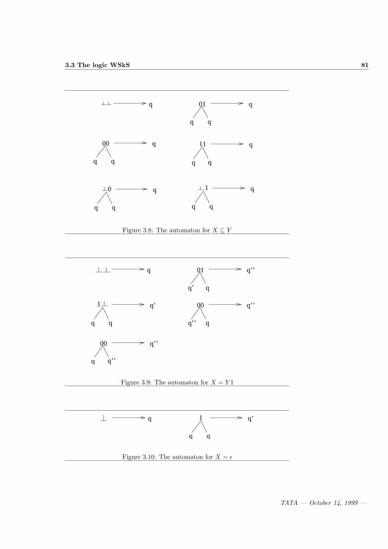
3.3 The logic WSkS 81
q
1
q q
q
00
q q
q q
11
0
q q
q
q q
q01
Figure 3.8: The automaton for X ⊆ Y
q
00
q’’
q’’1
q
q
01
q q
q’
q’
q’’
00 q’’
q q’’
Figure 3.9: The automaton for X = Y 1
q
q
1 q’
q
Figure 3.10: The automaton for X = ε
TATA — October 14, 1999 —
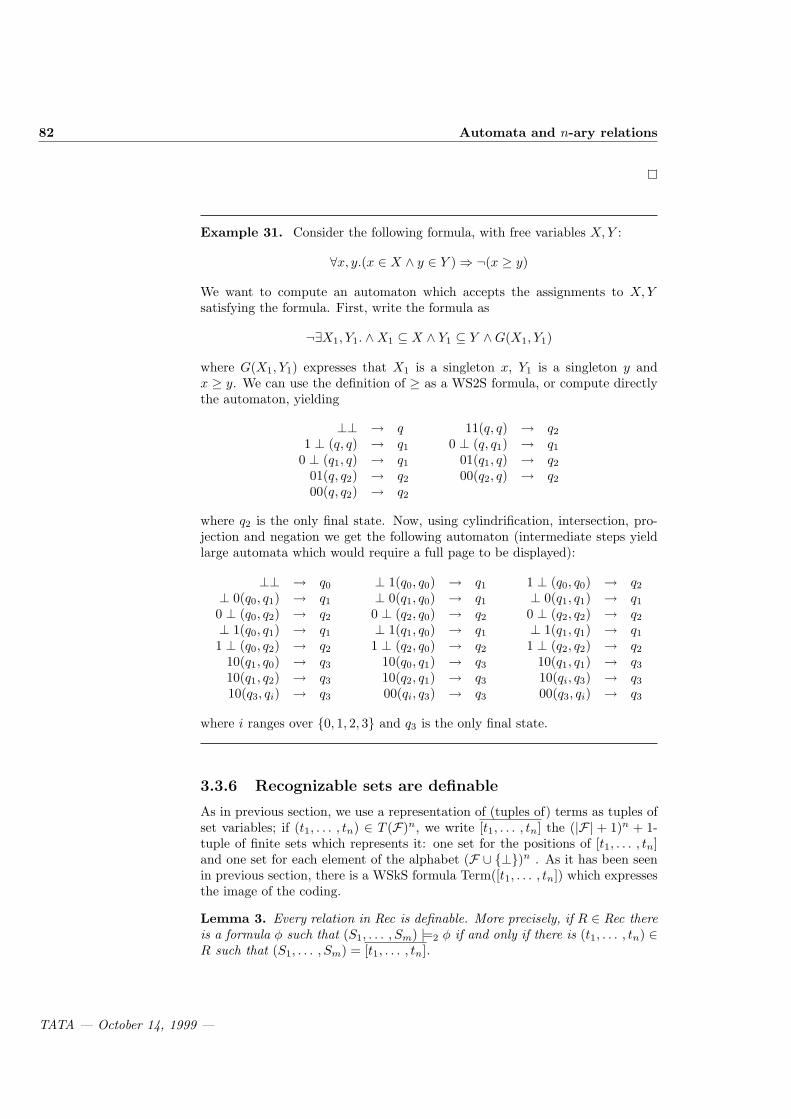
82 Automata and n-ary relations
Example 31. Consider the following formula, with free variables X,Y :
∀x, y.(x ∈ X ∧ y ∈ Y ) ⇒ ¬(x ≥ y)
We want to compute an automaton which accepts the assignments to X, Ysatisfying the formula. First, write the formula as
¬∃X1, Y1. ∧X1 ⊆ X ∧ Y1 ⊆ Y ∧G(X1, Y1)
where G(X1, Y1) expresses that X1 is a singleton x, Y1 is a singleton y andx ≥ y. We can use the definition of ≥ as a WS2S formula, or compute directlythe automaton, yielding
⊥⊥ → q 11(q, q) → q2
1 ⊥ (q, q) → q1 0 ⊥ (q, q1) → q1
0 ⊥ (q1, q) → q1 01(q1, q) → q2
01(q, q2) → q2 00(q2, q) → q2
00(q, q2) → q2
where q2 is the only final state. Now, using cylindrification, intersection, pro-jection and negation we get the following automaton (intermediate steps yieldlarge automata which would require a full page to be displayed):
⊥⊥ → q0 ⊥ 1(q0, q0) → q1 1 ⊥ (q0, q0) → q2
⊥ 0(q0, q1) → q1 ⊥ 0(q1, q0) → q1 ⊥ 0(q1, q1) → q1
0 ⊥ (q0, q2) → q2 0 ⊥ (q2, q0) → q2 0 ⊥ (q2, q2) → q2
⊥ 1(q0, q1) → q1 ⊥ 1(q1, q0) → q1 ⊥ 1(q1, q1) → q1
1 ⊥ (q0, q2) → q2 1 ⊥ (q2, q0) → q2 1 ⊥ (q2, q2) → q2
10(q1, q0) → q3 10(q0, q1) → q3 10(q1, q1) → q3
10(q1, q2) → q3 10(q2, q1) → q3 10(qi, q3) → q3
10(q3, qi) → q3 00(qi, q3) → q3 00(q3, qi) → q3
where i ranges over 0, 1, 2, 3 and q3 is the only final state.
3.3.6 Recognizable sets are definable
As in previous section, we use a representation of (tuples of) terms as tuples ofset variables; if (t1, . . . , tn) ∈ T (F)n, we write [t1, . . . , tn] the (|F| + 1)n + 1-tuple of finite sets which represents it: one set for the positions of [t1, . . . , tn]and one set for each element of the alphabet (F ∪ ⊥)n . As it has been seenin previous section, there is a WSkS formula Term([t1, . . . , tn]) which expressesthe image of the coding.
Lemma 3. Every relation in Rec is definable. More precisely, if R ∈ Rec thereis a formula φ such that (S1, . . . , Sm) |=2 φ if and only if there is (t1, . . . , tn) ∈R such that (S1, . . . , Sm) = [t1, . . . , tn].
TATA — October 14, 1999 —

3.3 The logic WSkS 83
Proof. Let A be the automaton which accepts the set of terms [t1, . . . , tn] for(t1, . . . , tn) ∈ R. The terminal alphabet of A is F ′ = (F ∪ ⊥)n, the setof states Q, the final states Qf and the set of transition rules T . Let F ′ =f1, . . . , fm and Q = q1, . . . , ql. The following formula φA (with m + 1 freevariables) defines the set [t1, . . . , tn] | (t1, . . . , tn) ∈ R.
∃Yq1 , . . . , ∃Yql.
Term(X, Xf1 , . . . , Xfm)∧ Partition(X,Yq1 , . . . , Yql
)∧ ∨
q∈Qfε ∈ Yq
∧ ∀x.∧
f∈F ′
∧
q∈Q
((x ∈ Xf ∧ x ∈ Yq) ⇒ (∨
f(q1,... ,qs)→q∈T
s∧
i=1
xi ∈ Yqi))
This formula basically expresses that there is a successful run of the automatonon [t1, . . . , tn]: the variables Yqi correspond to sets of positions which are labeledwith qi by the run. They should be a partition of the set of positions. The roothas to be labeled with a final state (the run is successful). Finally, the last lineexpresses local properties that have to be satisfied by the run: if the sons xi ofa position x are labeled with q1, ..., qn respectively and x is labeled with symbolf and state q, then there should be a transition f(q1, . . . , qn) → q in the set oftransitions.
We have to prove two inclusions. First assume that (S, S1, . . . , Sm) |=2 φ.Then (S, S1, . . . , Sm) |= Term(X,Xf1 , . . . , Xfm), hence there is a term u ∈T (F)′ whose set of position is S and such that for all i, Si is the set of positionslabeled with fi. Now, there is a partition Eq1 , . . . , Eql
of S which satisfies
S, S1, . . . , Sm, Eq1 , . . . , Eql|=
∀x.∧
f∈F ′
∧
q∈Q
((x ∈ Xf ∧ x ∈ Yq) ⇒ (∨
f(q1,... ,qs)→q∈T
s∧
i=1
xi ∈ Yqi))
This implies that the labeling Eq1 , . . . , Eqlis compatible with the transition
rules: it defines a run of the automaton. Finally, the condition that the root Λbelongs to Eqf
for some final state qf implies that the run is successful, hencethat u is accepted by the automaton.
Conversely, if u is accepted by the automaton, then there is a successful runof A on u and we can label its positions with states in such a way that thislabeling is compatible with the transition rules in A.
Putting together Lemmas 2 and 3, we can state the following slogan (whichis not very precise; the precise statements are given by the lemmas):
Theorem 21. L is definable if and only if L is in Rec.
And, as a consequence:
Theorem 22 ([TW68]). WSkS is decidable.
Proof. Given a formula φ of WSkS, by Lemma 2, we can compute a finite treeautomaton which has the same solutions as φ. Now, assume that φ has no freevariable. Then the alphabet of the automaton is empty (or, more precisely, it
TATA — October 14, 1999 —

84 Automata and n-ary relations
contains the only constant > according to what we explained in Section 3.2.4).Finally, the formula is valid iff the constant > is in the language, i.e. iff thereis a rule > −→ qf for some qf ∈ Qf .
3.3.7 Complexity issues
We have seen in chapter 1 that, for finite tree automata, emptiness can be de-cided in linear time (and is PTIME-complete) and that inclusion is EXPTIME-complete. Considering WSkS formulas with a fixed number of quantifiers al-ternations N , the decision method sketched in the previous section will workin time which is a tower of exponentials, the height of the tower being O(N).This is so because each time we encounter a sequence ∀X, ∃Y , the existentialquantification corresponds to a projection, which may yield a non-deterministicautomaton, even if the input automaton was deterministic. Then the eliminationof ∀X requires a determinization (because we have to compute a complementautomaton) which requires in general exponential time and exponential space.
Actually, it is not really possible to do much better since, even when k = 1,deciding a formula of WSkS requires non-elementary time, as shown in [SM73].
3.3.8 Extensions
There are several extensions of the logic, which we already mentioned: thoughquantification is restricted to finite sets, we may consider infinite sets as models(this is what is often called weak second-order monadic logic with k successorsand also written WSkS), or consider quantifications on arbitrary sets (this isthe full SkS).
These logics require more sophisticated automata which recognize sets ofinfinite terms. The proof of Theorem 22 carries over these extensions, with theprovision that the devices enjoy the required closure and decidability properties.But this becomes much more intricate in the case of infinite terms. Indeed, forinfinite terms, it is not possible to design bottom-up tree automata. We have touse a top-down device. But then, as mentioned in chapter 1, we cannot expectto reduce the non-determinism. Now, the closure by complement becomes prob-lematic because the usual way of computing the complement uses reduction ofnon-determinism as a first step.
It is out of the scope of this book to define and study automata on infiniteobjects (see [Tho90] instead). Let us simply mention that the closure under com-plement for Rabin automata which work on infinite trees (this result is knownas Rabin’s Theorem) is one of the most difficult results in the field
3.4 Examples of applications
3.4.1 Terms and sorts
The most basic example is what is known in the algebraic specification commu-nity as order-sorted signatures . These signatures are exactly what we calledbottom-up tree automata. There are only differences in the syntax. For in-
TATA — October 14, 1999 —

3.4 Examples of applications 85
stance, the following signature:
SORTS:Nat, intSUBSORTS : Nat ≤ intFUNCTION DECLARATIONS:
0 : → Nat+ : Nat× Nat → Nats : Nat → Natp : Nat → int+ : int× int → intabs : int → Natfact : Nat → Nat. . .
is an automaton whose states are Nat, int with an ε-transition from Nat to intand each function declaration corresponds to a transition of the automaton. Forexample +(Nat, Nat) → Nat. The set of well-formed terms (as in the algebraicspecification terminology) is the set of terms recognized by the automaton inany state.
More general typing systems also correspond to more general automata (aswill be seen e.g. in the next chapter).
This correspondence is not surprising; types and sorts are introduced in orderto prevent run-time errors by some “abstract interpretation” of the inputs. Treeautomata and tree grammars also provide such a symbolic evaluation mecha-nism. For other applications of tree automata in this direction, see e.g. chapter5.
From what we have seen in this chapter, we can go beyond simply recogniz-ing the set of well-formed terms. Consider the following sort constraints (thealphabet F of function symbols is given):
The set of sort expressions SE is the least set such that
• SE contains a finite set of sort symbols S, including the two particularsymbols >S and ⊥S .
• If s1, s2 ∈ SE , then s1 ∨ s2, s1 ∧ s2, ¬s1 are in SE
• If s1, . . . , sn are in SE and f is a function symbol of arity n, then f(s1, . . . , sn) ∈SE .
The atomic formulas are expressions t ∈ s where t ∈ T (F ,X ) and s ∈ SE .The formulas are arbitrary first-order formulas built on these atomic formulas.
These formulas are interpreted as follows: we are giving an order-sorted sig-nature (or a tree automaton) whose set of sorts is S. We define the interpretation[[·]]Sof sort expressions as follows:
• if s ∈ S, [[s]]S is the set of terms in T (F) that are accepted in state s.
• [[>S ]]S = T (F) and [[⊥S ]]S = ∅
• [[s1 ∨ s2]]S = [[s1]]S ∪ [[s2]]S , [[s1 ∧ s2]]S = [[s1]]S ∩ [[s2]]S , [[¬s]]S = T (F) \ [[s]]S
• [[f(s1, . . . , sn)]]S = f(t1, . . . , tn) | t1 ∈ [[s1]]S , . . . tn ∈ [[sn]]S
TATA — October 14, 1999 —

86 Automata and n-ary relations
t
u
Figure 3.11: u encompasses t
An assignment σ, mapping variables to terms in T (F), satisfies t ∈ s (wealso say that σ is a solution of t ∈ s) if tσ ∈ [[s]]S . Solutions of arbitrary formulasare defined as expected. Then
Theorem 23. Sort constraints are decidable.
The decision technique is based on automata computations, following theclosure properties of Rec× and a decomposition lemma for constraints of theform f(t1, . . . , tn) ∈ s.
More results and applications of sort constraints are discussed in the biblio-graphic notes.
3.4.2 The encompassment theory for linear terms
Definition 9. If t ∈ T (F ,X ) and u ∈ T (F), u encompasses t if there is asubstitution σ such that tσ is a subterm of u. (See Figure 3.11.) This bi-nary relation is denoted t ·£u or, seen as a unary relation on ground termsparametrized by t: ·£t(u).
Encompassment plays an important role in rewriting: a term t is reducibleby a term rewriting system R if and only if t encompasses at least one left handside of a rule.
The relationship with tree automata is given by the proposition:
Proposition 15. If t is linear, then the set of terms that encompass t is recog-nized by an NFTA of size O(|t|).Proof. To each non-variable subterm v of t we associate a state qv. In additionwe have a state q>. The only final state is qt. The transition rules are:
• f(q>, . . . , q>) → q> for all function symbols.
• f(qt1 , . . . , qtn) → qf(t1,... ,tn) if f(t1, . . . , tn) is a subterm of t and qti isactually q> is ti is a variable.
• f(q> . . . , q>, qt, q>, . . . , q>) → qt for all function symbols f whose arity isat least 1.
The proof that this automaton indeed recognizes the set of terms that encompasst is left to the reader.
TATA — October 14, 1999 —

3.4 Examples of applications 87
Note that the automaton may be non deterministic.
Corollary 4. If R is a term rewriting system whose all left members are linear,then the set of reducible terms in T (F), as well as the set of irreducible termsin T (F) are recognized by a finite tree automaton.
Proof. This is a consequence of Theorem 5.
The theory of reducibility associated with a set of term S ⊆ T (F ,X ) is theset of first-order formulas built on the unary predicate symbols Et, t ∈ S andinterpreted as the set of terms encompassing t.
Theorem 24. The reducibility theory associated with a set of linear terms isdecidable.
Proof. By Proposition 14, the set of solutions of an atomic formula is recog-nizable, hence definable in WSkS by Lemma 3. Hence, any first-order formulabuilt on these atomic predicate symbols can be translated into a (second-order)formula of WSkS which has the same models (up to the coding of terms intotuples of sets). Then, by Theorem 22, the reducibility theory associated with aset of linear terms is decidable.
Note however that we do not use here the full power of WSkS. Actually,the solutions of a Boolean combination of atomic formulas are in Rec×. So, wecannot apply the complexity results for WSkS here. (In fact, the complexity ofthe reducibility theory is unknown so far).
Let us simply show an example of an interesting property of rewrite systemswhich can be expressed in this theory.
Definition 10. Given a term rewriting system R, a term t is ground reducibleif, for every ground substitution σ, tσ is reducible by R.
Note that a term might be irreducible and still ground reducible. For in-stance consider the alphabet F = 0, s and the rewrite system R = s(s(0)) →0. Then the term s(s(x) is irreducible by R, but all its ground instances arereducible.
It turns out that ground reducibility of t is expressible in the encompassmenttheory by the formula:
∀x.( ·£t(x) ⇒n∨
i=1
·£li(x))
Where l1, . . . , ln are the left hand sides of the rewrite system. By Theorem24, if t, l1, . . . , ln are linear, then ground reducibility is decidable. Actually, ithas been shown that this problem is EXPTIME-complete, but is beyond thescope of this book to give the proof.
TATA — October 14, 1999 —

88 Automata and n-ary relations
3.4.3 The first-order theory of a reduction relation: thecase where no variables are shared
We consider again an application of tree automata to decision problem in logicand term rewriting.
Consider the following logical theory. Let L be the set of all first-orderformulas using no function symbols and a single binary predicate symbol →.
Given a rewrite system R, interpreting → as −→R
, yields the theory of one
step rewriting; interpreting → as ∗−→R
yields the theory of rewriting.
Both theories are undecidable for arbitrary R. They become however decid-able if we restrict our attention to term rewriting systems in which each variableoccurs at most once. Basically, the reason is given by the following:
Proposition 16. If R is a linear rewrite system such that left and right mem-bers of the rules do not share variables, then ∗−→
Ris recognized by a GTT.
Proof. As in the proof of Proposition 15, we can construct in linear time a(non-deterministic) automaton which accepts the set of instances of a linearterm. For each rule li → ri we can construct a pair (Ai,A′i) of automata whichrespectively recognize the set of instances of li and the set of instances of ri.Assume that the sets of states of the Ais are pairwise disjoint and that eachAi has a single final state qi
f . We may assume a similar property for the A′is:they do not share states and for each i, the only common state between Ai andA′i is qi
f (the final state for both of them). Then A (resp. A′) is the union ofthe Ais: the states are the union of all sets of states of the Ais (resp. A′is),transitions and final states are also unions of the transitions and final states ofeach individual automaton.
We claim that (A,A′) defines a GTT whose closure by iteration (A∗,A′∗)(which is again a GTT according to Theorem 20) accepting ∗−→
R. For, assume
first that up−−−−→
li→ri
v. Then u|p is an instance liσ of li, hence is accepted in state
qif . v|p is an instance riθ of ri, hence accepted in state qi
f . Now, v = u[riθ]p,hence (u, v) is accepted by the GTT (A,A′). It follows that if u
∗−→R
v, (u, v) is
accepted by (A∗,A′∗).Conversely, assume that (u, v) is accepted by (A,A′), then
u∗−→A
C[q1, . . . , qn]p1,... ,pn
∗←−−A′
v
Moreover, each qi is some state qjf , which, by definition, implies that u|pi is an
instance of lj and v|pi is an instance of rj . Now, since lj and rj do not sharevariables, for each i, u|pi −→R v|pi . Which implies that u
∗−→R
v. Now, if (u, v) is
accepted by (A∗,A′∗), u can be rewritten in v by the transitive closure of ∗−→R
,
which is ∗−→R
itself.
Theorem 25. If R is a linear term rewriting system such that left and rightmembers of the rules do not share variables, then the first-order theory of rewrit-ing is decidable.
TATA — October 14, 1999 —

3.4 Examples of applications 89
Proof. By Proposition 16, ∗−→R
is recognized by a GTT. From Proposition
9, ∗−→R
is in Rec. By Lemma 3, there is a WSkS formula whose solutions are
exactly the pairs (s, t) such that s∗−→R
t. Finally, by Theorem 22, the first-order
theory of ∗−→R
is decidable.
3.4.4 Reduction strategies
So far, we gave examples of first-order theories (or constraint systems) whichcan be decided using tree automata techniques. Other examples will be givenin the next two chapters. We give here another example of application in adifferent spirit: we are going to show how to decide the existence (and com-pute) “optimal reduction strategies” in term rewriting systems. Informally, areduction sequence is optimal when every redex which is contracted along thissequence has to be contracted in any reduction sequence yielding a normal form.For example, if we consider the rewrite system x ∨> → >;>∨ x → >, thereis no optimal sequential reduction strategy in the above sense since, given anexpression e1 ∨ e2, where e1 and e2 are unevaluated, the strategy should spec-ify which of e1 or e2 has to be evaluated first. However, if we start with e1,then maybe e2 will reduce to > and the evaluation step on e1 was unnecessary.Symmetrically, evaluating e2 first may lead to unnecessary computations. Aninteresting question is to give sufficient criteria for a rewrite system to admitoptimal strategies and, in case there is such a strategy, give it explicitly.
The formalization of these notions was given by Huet and Levy in [HL91]who introduce the notion of sequentiality. We give briefly a summary of (partof) their definitions.
F is a fixed alphabet of function symbols and FΩ = F ∪Ω is the alphabetF enriched with a new constant Ω (whose intended meaning is “unevaluatedterm”).
We define on T (FΩ) the relation “less evaluated than” as:
u v v if and only if either u = Ω or else u = f(u1, . . . , un), v =f(v1, . . . , vn) and for all i, ui v vi
Definition 11. A predicate P on T (FΩ) is monotonic if u ∈ P and u v vimplies v ∈ P .
For example, a monotonic predicate of interest for rewriting is the predicateNR: t ∈ NR if and only if there is a term u ∈ T (F) such that u is irreducibleby R and t
∗−→R
u.
Definition 12. Let P be a monotonic predicate on T (FΩ). If R is a termrewriting system and t ∈ T (FΩ), a position p of Ω in t is an index for P if forall terms u ∈ T (FΩ) such that t v u and u ∈ P , then u|p 6= Ω
In other words: it is necessary to evaluate t at position p in order to havethe predicate P satisfied.
Example 32. Let R = f(g(x), y) → g(f(x, y)); f(a, x) → a; b → g(b).Then 1 is an index of f(Ω, Ω) for NR: any reduction yielding a normal form
TATA — October 14, 1999 —
90 Automata and n-ary relations
without Ω will have to evaluate the term at position 1. More formally, everyterm f(t1, t2) which can be reduced to a term in T (F) in normal form satisfiest1 6= Ω. On the contrary, 2 is not an index of f(Ω,Ω) since f(a, Ω) ∗−→
Ra.
Definition 13. A monotonic predicate P is sequential if every term t such that:
• t /∈ P
• there is u ∈ T (F), t v u and u ∈ P
has an index for P .
If NR is sequential, the reduction strategy consisting of reducing an indexis optimal for non-overlapping and left linear rewrite systems.
Now, the relationship with tree automata is given by the following result:
Theorem 26. If P is definable in WSkS, then the sequentiality of P is alsodefinable in WSkS.
The proof of this result is quite easy: it suffices to translate directly thedefinitions.
For instance, if R is a rewrite system whose left and right members donot share variables, then NR is recognizable (by Propositions 16 and 9), hencedefinable in WSkS by Lemma 3 and the sequentiality of R is decidable byTheorem 26.
In general, the sequentiality of NR is undecidable. However, one can noticethat, if R and R′ are two rewrite systems such that −→
R⊆ −−→
R′, then a
position p which is an index for R′ is also an index for R. (And thus, R issequential whenever R′ is sequential).
For instance, we may approximate the term rewriting system, replacing allright hand sides by a new variable which does not occur in the correspondingleft member. LetR? be this approximation and N? be the predicate NR?. (Thisis the approximation considered by Huet and Levy).
Another, refined, approximation consists in renaming all variables of theright hand sides of the rules in such a way that all right hand sides becomelinear and do not share variables with their left hand sides. Let R′ be such anapproximation of R. The predicate NFR′ is written NV .
Proposition 17. If R is left linear, then the predicates NF? and NV are de-finable in WSkS and their sequentiality is decidable.
Proof. The approximations R? and R′ satisfy the hypotheses of Proposition 16and hence ∗−−→
R?and ∗−−→
R′are recognized by GTTs. On the other hand, the
set of terms in normal form for a left linear rewrite system is recognized by afinite tree automaton (see Corollary 4). By Proposition 9 and Lemma 3, allthese predicates are definable in WSkS. Then N? and NV are also definable inWSkS. For instance for NV :
NV (t) def= ∃u.t∗−−→R′
u ∧NF (u)
Then, by Theorem 26, the sequentiality of N? and NV are definable inWSkS and by Theorem 22 they are decidable.
TATA — October 14, 1999 —

3.4 Examples of applications 91
3.4.5 Application to rigid E-unification
Given a (universally quantified) set of equations E, the classical problem of E-unification is, given an equation s = t, find substitutions σ such that E |= sσ =tσ. The associated decision problem is to decide whether such a substitutionexists. This problem is in general unsolvable: there are decision procedures forrestricted classes of axioms E.
The simultaneous rigid E-unification problem is slightly different: we arestill giving E and a finite set of equations si = ti and the question is to find asubstitution σ such that
|= (∧
e∈E
eσ) ⇒ (n∧
i=1
siσ = tiσ)
The associated decision problem is to decide the existence of such a substitution.The relevance of such questions to automated deduction is very briefly de-
scribed in the bibliographic notes. We want here to show how tree automatahelp in this decision problem.
Simultaneous rigid E-unification is undecidable in general. However, for theone variable case, we have:
Theorem 27. The simultaneous rigid E-unification problem with one variableis EXPTIME-complete.
The EXPTIME membership is a direct consequence of the following lemma,together with closure and decision properties for recognizable tree languages.The EXPTIME-hardness is obtained by reduction the intersection non-emptinessproblem, see Theorem 11).
Lemma 4. The solutions of a rigid E-unification problem with one variable arerecognizable by a finite tree automaton.
Proof. (sketch) Assume that we have a single equation s = t. Let x be the onlyvariable occurring in E, s = t and E be the set E in which x is considered as aconstant. Let R be a canonical ground rewrite system associated with E (andfor which x is minimal). We define v as x if s and t have the same normal formw.r.t. R and as the normal form of xσ w.r.t. R otherwise.
Assume Eσ |= sσ = tσ. If v 6≡ x, we have E ∪ x = v |= x = xσ. HenceE ∪x = v |= s = t in any case. Conversely, assume that E ∪x = v |= s = t.Then E ∪ x = xσ |= s = t, hence Eσ |= sσ = tσ.
Now, assume v 6≡ x. Then either there is a subterm u of an equation in Esuch that E |= u = v or else R1 = R ∪ v → x is canonical. In this case, fromE ∪v = x |= s = t, we deduce that either E |= s = t (and v ≡ x) or there is asubterm u of s, t such that E |= v = u. we can conclude that, in all cases, thereis a subterm u of E ∪ s = t such that E |= u = v.
To summarize, σ is such that Eσ |= sσ = tσ iff there is a subterm u ofE ∪ s = t such that E |= u = xσ and E ∪ u = x |= s = t.
If we let T be the set of subterms of E∪s = t such that E∪u = x |= s = t,then T is finite (and computable in polynomial time). The set of solutions isthen ∗−−−→
R−1(T ), which is a recognizable set of trees, thanks to Proposition 16.
Further comments and references are given in the bibliographic notes.
TATA — October 14, 1999 —

92 Automata and n-ary relations
3.4.6 Application to higher-order matching
We give here a last application (but the list is not closed!), in the typed lambda-calculus.
To be self-contained, let us first recall some basic definitions in typed lambdacalculus.
The set of types of the simply typed lambda calculus is the least set contain-ing the constant o (basic type) and such that τ → τ ′ is a type whenever τ andτ ′ are types.
Using the so-called Curryfication, any type τ → (τ ′ → τ ′′) is written τ, τ ′ →τ ′′. In this way all non-basic types are of the form τ1, . . . , τn → o with intuitivemeaning that this is the type of functions taking n arguments of respective typesτ1, . . . , τn and whose result is a basic type o.
The order of a type τ is defined by:
• O(o) = 1
• O(τ1, . . . , τn → o) = 1 + maxO(τ1), . . . , O(τn)Given, for each type τ a set of variables Xτ of type τ and a set Cτ of constants
of type τ , the set of terms (of the simply typed lambda calculus) is the leastset Λ such that:
• x ∈ Xτ is a term of type τ
• c ∈ Cτ is a term of type τ
• If x1 ∈ Xτ1 , . . . , xn ∈ Xτn and t is a term of type τ , then λx1, . . . xn : t isa term of type τ1, . . . , τn → τ
• If t is a term of type τ1, . . . , τn → τ and t1, . . . , tn are terms of respectivetypes τ1, . . . , τn, then t(τ1, . . . , τn) is a term of type τ .
The order of a term t is the order of its type τ(t).The set of free variables Var(t) of a term t is defined by:
• Var(x) = x if x is a variable
• Var(c) = ∅ if c is a constant
• Var(λx1 . . . , xn : t) = Var(t) \ x1, . . . , xn• Var(t(u1, . . . , un)) = Var(t) ∪ Var(t1) ∪ . . . ∪ Var(tn)
Terms are always assumed to be in η-long form, i.e. they are assumed tobe in normal form with respect to the rule:
(η) t → λx1 . . . xn.t(x1, . . . , xn) if τ(t) = τ1, . . . τn → τand xi ∈ Xτi \ Var(t) for all i
We define the α-equivalence =α on Λ as the least congruence relation suchthat: λx1, . . . , xn : t =α λx′1 . . . , x′n : t′ when
• t′ is the term obtained from t by substituting for every index i, every freeoccurrence of xi with x′i.
TATA — October 14, 1999 —

3.4 Examples of applications 93
• There is no subterm of t in which, for some index i, both xi and x′i occurfree.
In the following, we consider only lambda terms modulo α-equivalence. Thenwe may assume that, in any term, any variable is bounded at most once andfree variables do not have bounded occurrences.
The β-reduction is defined on Λ as the least binary relation −→β
such that
• λx1 . . . xn : t(t1, . . . , tn) −→β
tx1←t1, . . . , xn←tn
• for every context C, C[t] −→β
C[u] whenever t −→β
u
It is well-known that βη-reduction is terminating and confluent on Λ and,for every term t ∈ Λ, we let t ↓ be the unique normal form of t.
A matching problem is an equation s = t where s, t ∈ Λ and Var(t) = ∅.A solution of a matching problem is a substitution σ of the free variables of tsuch that sσ ↓= t ↓.
Whether or not the matching problem is decidable is an open question at thetime we write this book. However, it can be decided when every free variableoccurring in s is of order less or equal to 4. We sketch here how tree automatamay help in this matter. We will consider only two special cases here, leaving thegeneral case as well as details of the proofs as exercises (see also bibliographicnotes).
First consider a problem
(1) x(s1, . . . , sn) = t
where x is a third order variable and s1, . . . , sn, t are terms without free vari-ables.
The first result states that the set of solutions is recognizable by a 2-automaton. 2-automata are a slight extension of finite tree automata: weassume here that the alphabet contains a special symbol 2. Then a term u isaccepted by a 2-automaton A if and only if there is a term v which is accepted(in the usual sense) by A and such that u is obtained from v by replacing eachoccurrence of the symbol 2 with a term (of appropriate type). Note that twodistinct occurrences of 2 need not to be replaced with the same term.
We consider the automaton As1,... ,sn,t defined by: F consists of all symbolsoccurring in t plus the variable symbols x1, . . . , xn whose types are respectivelythe types of s1, . . . , sn and the constant 2.
The set of states Q consists of all subterms of t, which we write qu (insteadof u) and a state q2. In addition, we have the final state qf .
The transition rules ∆ consist in
• The rules
f(qt1 , . . . , qtn) → qf(t1,... ,tn)
each time qf(t1,... ,tn) ∈ Q
• For i = 1, . . . , n, the rules
xi(qt1 , . . . , qtn) → qu
where u is a subterm of t such that si(t1, . . . , tn) ↓= u and tj = 2 when-ever si(t1, . . . , tj−1,2, tj+1, . . . , tn) ↓= u.
TATA — October 14, 1999 —

94 Automata and n-ary relations
• the rule λx1, . . . , λxn.qt → qf
Theorem 28. The set of solutions of (1) (up to α-conversion) is accepted bythe 2-automaton As1,... ,sn,t.
More about this result, its proof and its extension to fourth order will begiven in the exercises (see also bibliographic notes). Let us simply give anexample.
Example 33. Let us consider the interpolation equation
x(λy1λy2.y1, λy3.f(y3, y3)) = f(a, a)
where y1, y2 are assumed to be of base type o. Then F = a, f, x1,2o. Q =qa, qf(a,a), q2o and the rules of the automaton are:
a → qa f(qa, qa) → qf(a,a)
2o → q2o x1(qa, q2o) → qa
x1(qf(a,a), q2o) → qf(a,a) x2(qa) → qf(a,a)
λx1λx2.qf(a,a) → qf
For instance the term λx1λx2.x1(x2(x1(x1(a,2o), 2o)),2o) is accepted bythe automaton :
λx1λx2.x1(x2(x1(x1(a,2o), 2o)),2o)∗−→A
λx1λx2.x1(x2(x1(x1(qa, q2o), q2o)), q2o)
−→A
λx1λx2.x1(x2(x1(qa, q2o)), q2o)
−→A
λx1λx2.x1(x2(qa), q2o)
−→A
λx1λx2.x1(qf(a,a), q2o)
−→A
λx1λx2.qf(a,a)
−→A
qf
And indeed, for every terms t1, t2, t3, λx1λx2.x1(x2(x1(x1(a, t1), t2)), t3) is asolution of the interpolation problem.
3.5 Exercises
Exercise 31. Let F be the alphabet consisting of finitely many unary functionsymbols a1, . . . , an and a constant 0.
1. Show that the set S of pairs (of words) (an1 (a1(a2(a
p2(0)))), an
1 (ap2(0))) | n, p ∈
N is in Rec. Show that S∗ is not in Rec, hence that Rec is not closed undertransitive closure.
2. More generally, show that, for any finite rewrite system R (on the alphabet F!), the reduction relation −→
Ris in Rec.
3. Is there any hope to design a class of tree languages which contains Rec, which isclosed by all Boolean operations and by transitive closure and for which empti-ness is decidable ? Why ?
TATA — October 14, 1999 —

3.5 Exercises 95
Exercise 32. Show that the set of pairs (t, f(t, t′)) | t, t′ ∈ T (F) is not in Rec.
Exercise 33. Show that if a binary relation is recognized by a GTT, then its inverse
is also recognized by a GTT.
Exercise 34. Give an example of two relations that are recognized by GTTs andwhose union is not recognized by any GTT.
Similarly, show that the class of relations recognized by a GTT is not closed bycomplement. Is the class closed by intersection ?
Exercise 35. Give an example of a n-ary relation such that its ith projection followed
by its ith cylindrification does not give back the original relation. On the contrary,
show that ith cylindrification followed by ith projection gives back the original relation.
Exercise 36. About Rec and bounded delay relations. We assume that F onlycontains unary function symbols and a constant, i.e. we consider words rather thantrees and we write u = a1 . . . an instead of u = a1(. . . (an(0)) . . . ). Similarly, u · vcorresponds to the usual concatenation of words.
A binary relation R on T (F) is called a bounded delay relation if and only if
∃k/∀(u, v) ∈ R, |u| − |v| ≤ k
R preserves the length if and only if
∀(u, v) ∈ R, |u| = |v|If A, B are two binary relations, we write A ·B (or simply AB) the relation
A ·B def= (u, v)/∃(u1, v1) ∈ A, (u2, v2) ∈ Bu = u1.u2, v = v1.v2
Similarly, we write (in this exercise !)
A∗ = (u, v)/∃(u1, v1) ∈ A, . . . , (un, vn) ∈ A, u = u1 . . . un, v = v1 . . . vn
1. Given A, B ∈ Rec, is A ·B necessary in Rec ? is A∗ necessary in Rec ? Why ?
2. Show that if A ∈ Rec preserves the length, then A∗ ∈ Rec.
3. Show that if A, B ∈ Rec and A is of bounded delay, then A ·B ∈ Rec.
4. The family of rational relations is the smallest set of subsets of T (F)2 which con-tains the finite subsets of T (F)2 and which is closed under union, concatenation(·) and ∗.Show that, if A is a bounded delay rational relation, then A ∈ Rec. Is theconverse true ?
Exercise 37. Let R0 be the rewrite system x×0 → 0; 0×x → 0 and F = 0, 1, s,×1. Construct explicitly the GTT accepting
∗−−→R0
.
2. Let R1 = R0 ∪ x× 1 → x. Show that∗−−→
R1is is not recognized by a GTT.
3. Let R2 = R1 ∪ 1 × x → x × 1. Using a construction similar to the transitive
closure of GTTs, show that the set t ∈ T (F) | ∃u ∈ T (F), t∗−−→
R2u, u ∈ NF
where NF is the set of terms in normal form for R2 is recognized by a finitetree automaton.
TATA — October 14, 1999 —

96 Automata and n-ary relations
Exercise 38. (*) More generally, prove that given any rewrite system li → ri | 1 ≤i ≤ n such that
1. for all i, li and ri are linear
2. for all i, if x ∈ Var(li) ∩ Var(ri), then x occurs at depth at most one in li.
the set t ∈ T (F) | ∃u ∈ NF, t∗−→R
u is recognized by finite tree automaton.
What are the consequences of this result ?
(See [Jac96] for details about this results and its applications. Also compare with
Exercise 15, question 4.)
Exercise 39. Show that the set of pairs (f(t, t′), t) | t, t′ ∈ T (F) is not definable
in WSkS. (See also Exercise 32)
Exercise 40. Show that the set of pairs of words (w, w′) | l(w) = l(w′), where l(x)
is the length of x, is not definable in WSkS.
Exercise 41. Let F = a1, . . . , an, 0 where each ai is unary and 0 is a constant.Consider the following constraint system: terms are built on F , the binary symbols∩,∪, the unary symbol ¬ and set variables. Formulas are conjunctions of inclusionconstraints t ⊆ t′. The formulas are interpreted by assigning to variables finite subsetsof T (F), with the expected meaning for other symbols.
Show that the set of solutions of such constraints is in Rec2. What can we conclude?
(*) What happens if we remove the condition on the ai’s to be unary?
Exercise 42. Complete the proof of Proposition 13.
Exercise 43. Show that the subterm relation is not definable in WSkS.Given a term t Write a WSkS formula φt such that a term u |= φt if and only if t
is a subterm of u.
Exercise 44. Define in SkS “X is finite”. (Hint: express that every totally orderedsubset of X has an upper bound and use Konig’s lemma)
Exercise 45. A tuple (t1, . . . , tn) ∈ T (F)n can be represented in several ways asa finite sequence of finite sets. The first one is the encoding given in Section 3.3.6,overlapping the terms and considering one set for each tuple of symbols. A second oneconsists in having a tuple of sets for each component: one for each function symbol.
Compare the number of free variables which result from both codings when defining
an n-ary relation on terms in WSkS. Compare also the definitions of the diagonal ∆
using both encodings. How is it possible to translate an encoding into the other one
?
Exercise 46. (*) Let R be a finite rewrite system whose all left and right membersare ground.
1. Let Termination(x) be the predicate on T (F) which holds true on t when thereis no infinite sequence of reductions starting from t. Show that adding thispredicate as an atomic formula in the first-order theory of rewriting, this theoryremains decidable for ground rewrite systems.
2. Generalize these results to the case where the left members of R are linear andthe right members are ground.
Exercise 47. The complexity of automata recognizing the set of irreducible groundterms.
1. For each n ∈ N, give a linear rewrite system Rn whose size is O(n) and suchthat the minimal automaton accepting the set of irreducible ground terms hasa size O(2n).
TATA — October 14, 1999 —

3.5 Exercises 97
2. Assume that for any two strict subterms s, t of left hand side(s) of R, if s and tare unifiable, then s is an instance of t or t is an instance of s. Show that thereis a NFTA A whose size is linear in R and which accepts the set of irreducibleground terms.
Exercise 48. Prove Theorem 26.
Exercise 49. The Propositional Linear-time Temporal Logic. The logic PTLis defined as follows:
Syntax P is a finite set of propositional variables. Each symbol of P is a formula (anatomic formula). If φ and ψ are formulas, then the following are formulas:
φ ∧ ψ, φ ∨ ψ, φ → ψ, ¬φ, φUψ, Nφ, Lφ
Semantics Let P ∗ be the set of words over the alphabet P . A word w ∈ P ∗ isidentified with the sequence of letters w(0)w(1) . . . w(|w| − 1). w(i..j) is theword w(i) . . . w(j). The satisfaction relation is defined by:
• if p ∈ P , w |= p if and only if w(0) = p
• The interpretation of logical connectives is the usual one
• w |= Nφ if and only if |w| ≥ 2 and w(1..|w| − 1) |= φ
• w |= Lφ if and only if |w| = 1
• w |= φUψ if and only if there is an index i ∈ [0..|w|] such that for allj ∈ [0..i], w(j..|w| − 1) |= φ and w(i..|w| − 1) |= ψ.
Let us recall that the language defined by a formula φ is the set of words w suchthat w |= φ.
1. What it is the language defined by N(p1Up2) (with p1, p2 ∈ P ) ?
2. Give PTL formulas defining respectively P ∗p1P∗, p∗1, (p1p2)
∗.
3. Give a first-order WS1S formula (i.e. without second-order quantification andcontaining only one free second-order variable) which defines the same languageas N(p1Up2)
4. For any PTL formula, give a first-order WS1S formula which defines the samelanguage.
5. Conversely, show that any language defined by a first-order WS1S formula isdefinable by a PTL formula.
Exercise 50. About 3rd-order interpolation problems
1. Prove Theorem 28.
2. Show that the size of the automaton As1,... ,sn,t is O(n× |t|)3. Deduce from Exercise 18 that the existence of a solution to a system of interpo-
lation equations of the form x(s1, . . . , sn) = t (where x is a third order variablein each equation) is in NP.
Exercise 51. About general third order matching.
1. How is it possible to modify the construction of As1,... ,sn,t so as to forbid somesymbols of t to occur in the solutions ?
TATA — October 14, 1999 —

98 Automata and n-ary relations
2. Consider a third order matching problem u = t where t is in normal form anddoes not contain any free variable. Let x1, . . . , xn be the free variables of u andxi(s1, . . . , sm) be the subterm of u at position p. Show that, for every solutionσ, either u[2]pσ ↓=α t or else that xiσ(s1σ, . . . , smσ) ↓ is in the set Sp definedas follows: v ∈ Sp if and only if there is a subterm t′ of t and there are positionsp1, . . . , pk of t′ and variables z1, . . . , zk which are bound above p in u such thatv = t′[z1, . . . , zk]p1,... ,pk .
3. By guessing the results of xiσ(s1σ, . . . , smσ) and using the previous exercise,show that general third order matching is in NP.
Exercise 52. About fourth-order matching.
** a completer **
3.6 Bibliographic Notes
The following bibliographic notes only concern the applications of the usualfinite tree automata on finite trees (as defined at this stage of the book). Weare pretty sure that there are many missing references and we are pleased toreceive more pointers to the litterature.
3.6.1 GTT
GTT were introduced in [DTHL87] where they were used for the decidability ofconfluence of ground rewrite systems.
3.6.2 Automata and Logic
The development of automata in relation with logic and verification (in thesixties) is reported in [Tra95]. This research program was explained by A.Church himself in 1962 [Chu62].
Milestones of the decidability of monadic second-order logic are the papers[Buc60] [Rab69]. Theorem 22 is proved in [TW68].
3.6.3 Surveys
There are numerous surveys on automata and logic. Let us mention some ofthem: M.O. Rabin [Rab77] surveys the decidable theories; W. Thomas [Tho90,Tho97] provides an excellent survey of relationships between automata and logic.
3.6.4 Applications of tree automata to constraint solving
Concerning applications of tree automata, the reader is also referred to [Dau94]which reviews a number of applications of Tree automata to rewriting and con-straints.
The relation between sorts and tree automata is pointed out in [Com89]. Thedecidability of arbitrary first-order sort constraints (and actually the first ordertheory of finite trees with equality and sort constraints) is proved in [CD94].
More general sort constraints involving some second-order terms are studiedin [Com98b] with applications to a sort constrained equational logic [Com98a].
TATA — October 14, 1999 —

3.6 Bibliographic Notes 99
Sort constraints are also applied to specifications and automated inductiveproofs in [BJ97] where tree automata are used to represent some normal formssets. They are used in logic programming and automated reasoning [FSVY91,GMW97], in order to get more efficient procedures for fragments which fallinto the scope of tree automata techniques. They are also used in automateddeduction in order to increase the expressivity of (counter-)model constructions[Pel97].
Concerning encompassment, M. Dauchet et al gave a more general result(dropping the linearity requirement) in [DCC95]. We will come back to thisresult in the next chapter.
3.6.5 Application of tree automata to semantic unification
Rigid unification was originally considered by J. Gallier et al. [GRS87] whoshowed that this is a key notion in extending the matings method to a logicwith equality. Several authors worked on this problem and it is out of the scopeof this book to give a list of references. Let us simply mention that the resultof Section 3.4.5 can be found in [Vea97b]. Further results on application of treeautomata to rigid unification can be found in [DGN+98], [GJV98].
Tree automata are also used in solving classical semantic unification prob-lems. See e.g. [LM93] [KFK97] [Uri92]. For instance, in [KFK97], the idea isto capture some loops in the narrowing procedure using tree automata.
3.6.6 Application of tree automata to decision problemsin term rewriting
Some of the applications of tree automata to term rewriting follow from theresults on encompassment theory. Early works in this area are also mentionedin the bibliographic notes of Chapter 1. The reader is also referred to the survey[GT95].
The first-order theory of the binary (many-steps) reduction relation w.r.t.a ground rewrite system has been shown decidable by. M. Dauchet and S.Tison [DT90]. Extensions of the theory, including some function symbols, orother predicate symbols like the parallel rewriting or the termination predicate(Terminate(t) holds if there is no infinite reduction sequence starting from t),or fair termination etc... remain decidable [DT90]. **Mauvaise citation !? Seealso the exercises.
Both the theory of one step and the theory of many steps rewriting areundecidable for arbitrary R [Tre96].
Reduction strategies for term rewriting have been first studied by Huet andLevy in 1978 [HL91]. They show here the decidability of strong sequential-ity for orthogonal rewrite systems. This is based on an approximation of therewrite system which, roughly, only considers the left sides of the rules. Bet-ter approximation, yielding refined criteria were further proposed in [Oya93],[Com95], [Jac96]. The orthogonality requirement has also been replaced withthe weaker condition of left linearity. The first relation between tree automata,WSkS and reduction strategies is pointed out in [Com95]. Further studies ofcall-by-need strategies, which are still based on tree automata, but do not usea detour through monadic second-order logic can be found in [DM97]. For allthese works, a key property is the preservation of regularity by (many-steps)
TATA — October 14, 1999 —
100 Automata and n-ary relations
rewriting, which was shown for ground systems in [Bra69], for linear systemswhich do not share variables in [DT90], for shallow systems in [Com95], for rightlinear monadic rewrite systems [Sal88], for linear semi-monadic rewrite systems[CG90], also called (with slight differences) growing systems in [Jac96]. Grow-ing systems are the currently most general class for which the preservation ofrecognizability is known.
As already pointed out, the decidability of the encompassment theory impliesthe decidability of ground reducibility. There are several papers written alongthese lines which will be explained in the next chapter.
Finally, approximations of the reachable terms are computed in [Gen97]using tree automata techniques, which implies the decision of some safety prop-erties.
3.6.7 Other applications
The relationship between finite tree automata and higher-order matching isstudied in [CJ97].
Finite tree automata are also used in logic programming [FSVY91], typereconstruction [Tiu92] and automated deduction [GMW97].
For further applications of tree automata in the direction of program verifi-cation, see e.g. chapter 5 of this book or e.g. [Jon87].
TATA — October 14, 1999 —

Chapter 4
Automata with constraints
4.1 Introduction
A typical example of a language which is not recognized by a finite tree au-tomaton is the set of terms f(t, t) | t ∈ T (F). The reason is that the twosons of the root are recognized independently and only a fixed finite amount ofinformation can be carried up to the root position, whereas t may be arbitrar-ily large. Therefore, as seen in the application section of the previous chapter,this imposes some linearity conditions, typically when automata techniques areapplied to rewrite systems or to sort constraints. The shift from linear to nonlinear situations can also be seen as a generalization from tree automata to DAG(directed acyclic graphs) automata. This is the purpose of the present chapter:how is it possible to extend the definitions of tree automata in order to carryover the applications of the previous chapter to (some) non-linear situations ?
Such an extension has been studied in the early 80’s by M. Dauchet and J.Mongy. They define a class of automata which (when working in a top-downfashion) allow duplications. Considering bottom-up automata, this amounts tocheck equalities between subtrees. This yields the RATEG class . This classis not closed under complement. If we consider its closure, we get the classof automata with equality and disequality constraints. This class is studied inSection 4.2.
Unfortunately, the emptiness problem is undecidable for the class RATEG(and hence for automata with equality and disequality constraints).Several decidable subclasses have been studied in the literature. The mostremarkable ones are
• The class of automata with constraints between brothers which, roughly,allows equality (or disequality) tests only between positions with the sameancestors. For instance, the set of terms f(t, t) is recognized by suchan automaton. This class is interesting because all properties of treeautomata carry over this extension and hence most of the applications oftree automata can be extended, replacing linearity conditions with suchrestrictions on non-linearities.
We study this class in Section 4.3.
• The class of reduction automata which, roughly, allows arbitrary disequal-
TATA — October 14, 1999 —

102 Automata with constraints
ity constraints but only a fixed finite amount of equality constraints oneach run of the automaton. For instance the set of terms f(t, t) also be-longs to this class. Though closure properties have to be handled withcare (with the definition sketched above, the class is not closed by com-plement), reduction automata are interesting because for example the setof irreducible terms (w.r.t. an arbitrary, possibly non-linear rewrite sys-tem) is recognized by an reduction automaton. Then the decidability ofground reducibility is a direct consequence of emptiness decidability forreduction automata. There is also a logical counterpart: the reducibilitytheory which is presented in the linear case in the previous chapter andwhich can be shown decidable in the general case using a similar technique.
Reduction automata are studied in Section 4.4.
We also consider in this chapter automata with arithmetic constraints. Theynaturally appear when some function symbols are assumed to be associative andcommutative (AC). In such a situation, the sons of an AC symbol can be per-muted and the relevant information is then the number of occurrences of thesame subtree in the multisets of sons. These integer variables (number of occur-rences) are subject to arithmetic constraints which must belong to a decidablefragment of arithmetic in order to keep closure and decidability properties.
4.2 Automata with equality and disequality con-straints
4.2.1 The most general class
An equality constraint (resp. a disequality constraint) is a predicate onT (F) written π = π′ (resp. π 6= π′) where π, π′ ∈ 1, . . . , k∗. Such a predicateis satisfied on a term t, which we write t |= π = π′, if π, π′ ∈ Pos(t) and t|π = t|π′(resp. π 6= π′ is satisfied on t if π = π′ is not satisfied on t).
The satisfaction relation |= is extended as usual to any Boolean combinationof equality and disequality constraints. The empty conjunction and disjunctionare respectively written ⊥ (false) and > (true).
An automaton with equality and disequality constraints is a tuple(Q,F , Qf ,∆) where F is a finite ranked alphabet, Q is a finite set of states, Qf
is a subset of Q of finite states and ∆ is a set of transition rules of of the form
f(q1, . . . , qn) c−→ q
where f ∈ F , q1, . . . , qn, q ∈ Q, and c is a Boolean combination of equality(and disequality) constraints. The state q is called target state in the abovetransition rule.
We write for short AWEDC the class of automata with equality and dise-quality constraints.
Let A = (Q,F , Qf , ∆) ∈ AWEDC. The move relation →A is defined by asfor NFTA modulo the satisfaction of equality and disequality constraints: lett, t′ ∈ F (F ∪Q,X), then t→A t′ if and only
there is a context C ∈ C(F ∪Q) and some terms u1, . . . , un ∈ T (F)
TATA — October 14, 1999 —

4.2 Automata with equality and disequality constraints 103
there exists f(q1, . . . , qn) c−→ q ∈ ∆
t = C[f(q1(u1), . . . , qn(un)] and t′ = C[q(f(u1, . . . , un))]
C[f(u1, . . . , un)] |= c
∗→A is the reflexive and transitive closure of →A. As in Chapter 1, we usuallywrite t
∗→A q instead of t∗→A q(t).
An automaton A ∈ AWEDC accepts (or recognizes) a ground termt ∈ T (F) if t
∗→A q for some state q ∈ Qf . More generally, we also say thatA accepts t in state q iff t
∗→A q (acceptance by A is the particular case ofacceptance by A in a final state).
A run) is a mapping ρ from Pos(t) into ∆ such that:
• ρ(Λ) ∈ Qf
• if t(p) = f and the target state of ρ(p) is q, then there is a transition rulef(q1, . . . , qn) c−→ q in ∆ such that for all 1 ≤ i ≤ n, the target state of
ρ(pi) is qi and t|p |= c.
Note that we do not have here exactly the same definition of a run as inChapter 1: instead of the state, we keep also the rule which yielded this state.This will be useful in the design of an emptiness decision algorithm for non-deterministic automata with equality and disequality constraints.
The language accepted (or recognized) by an automaton A ∈ AWEDCis the set L(A) of terms t ∈ T (F) that are accepted by A.
Example 34. Balanced complete binary trees over the alphabet f (binary)and a (constant) are recognized by the AWEDC (q, f, a, q, ∆) where ∆consists of the following rules:
r1 : a → q
r2 : f(q, q) 1=2−−→ q
For example, t = f(f(a, a), f(a, a)) is accepted. The mapping which associatesr1 to every position p of t such that t(p) = a and which associates r2 to everyposition p of t such that t(p) = f is indeed a successful run: for every positionp of t such that t(p) = f , t|p·1 = tp·2, hence t|p |= 1 = 2.
Example 35. Consider the following AWEDC: (Q,F , Qf ,∆) with F =0, s, f where 0 is a constant, s is unary and f has arity 4, Q = qn, q0, qf,Qf = qf, and ∆ consists of the following rules:
0 → q0 s(q0) → qn
s(qn) → qn f(q0, q0, qn, qn) 3=4−−→ qf
f(q0, q0, q0, q0) → qf f(q0, qn, q0, qn) 2=4−−→ qf
f(qf , qn, qn, qn) 14=4∧21=12∧131=3−−−−−−−−−−−−−→ qf
TATA — October 14, 1999 —

104 Automata with constraints
s
s
s
f
f
f s
s
s
s
s
s
s
s
s
ss
sss
s0 0
0
0
0
0 0
0
0
0
Figure 4.1: A computation of the sum of two natural numbers
This automaton computes the sum of two natural numbers written in baseone in the following sense: if t is accepted byA then1 t = f(t1, sn(0), sm(0), sn+m(0))for some t1 and n,m ≥ 0. Conversely, for each n,m ≥ 0, there is a termf(t1, sn(0), sm(0), sn+m(0)) which is accepted by the automaton.
For instance the term depicted on Figure 4.1 is accepted by the automaton.Similarly, it is possible to design an automaton of the class AWEDC which“computes the multiplication” (see exercises)
In order to evaluate the complexity of operations on automata of the classAWEDC, we need to precise a representation of the automata and estimate thespace which is necessary for this representation.
The size of is a Boolean combination of equality and disequality constraintsis defined by induction:
• ‖π = π′‖ def= ‖π 6= π′‖ def= |π|+ |π′| (|π| is the length of π)
• ‖c ∧ c′‖ def= ‖c ∨ c′‖ def= ‖c‖+ ‖c′‖+ 1
• ‖¬c‖ def= ‖c‖
Now, deciding whether t |= c depends on the representation of t. If t isrepresented as a directed acyclic graph (a DAG) with maximal sharing, then thiscan be decided in O(‖c‖) on a RAM. Otherwise, it requires to compute first this
1sn(0) denotes s(. . . s| z n
(0)
TATA — October 14, 1999 —

4.2 Automata with equality and disequality constraints 105
representation of t, and hence can be computed in time at most O(‖t‖ log ‖t‖+‖c‖).
¿From now on, we assume, for complexity analysis, that the terms are rep-resented with maximal sharing in such a way that checking an equality or adisequality constraint on t can be completed in a time which is independent of‖t‖.
The size of an automaton A ∈ AWEDC is
‖A‖ def= |Q|+∑
f(q1,... ,qn)c−→ q∈∆
n + 2 + ‖c‖
An automaton A in AWEDC is deterministic if for every t ∈ T (F), thereis at most one state q such that t
∗−→A
q. It is complete if for every t ∈ T (F)
there is at least one state q such that t∗−→A
q.
When every constraint is a tautology, then our definition of automata re-duces to the definition of Chapter 1. However, in such a case, the notions ofdeterminacy do not fully coincide, as noticed in Chapter 1, page 17.
Proposition 18. Given t ∈ T (F) and A ∈AWEDC, deciding whether t is ac-cepted by A can be completed in polynomial time (linear time for a deterministicautomaton).
Proof. Because of the DAG representation of t, the satisfaction of a constraintπ = π′ on t can be completed in time O(|π| + |π′|). Thus, if A is determinis-tic, the membership test can be performed in time O(‖t‖ + ‖A‖ + MC ) whereMC = max(‖c‖ ∣∣ c is a constraint of a rule of A). If A is nondeterministic, thecomplexity of the algorithm will be O(‖t‖ × ‖A‖ ×MC ).
4.2.2 Reducing non-determinism and closure properties
Proposition 19. For every automaton A ∈ AWEDC, there is a complete au-tomaton A′ which accepts the same language as A. The size ‖A′‖ is polynomialin ‖A‖ and the computation of A′ can be performed in polynomial time (for afixed alphabet). If A is deterministic, then A′ is deterministic.
Proof. The proof is the same as for Theorem 2: we add a trash state andevery transition is possible to the trash state. However, this does not keep thedeterminism of the automaton. We need the following more careful computationin order to preserve the determinism.
We also add a single trash state q⊥. The additional transitions are computedas follows: for each function symbol f ∈ F and each tuple of states (including thetrash state) q1, . . . , qn, if there is no transition f(q1, . . . , qn) c−→ q ∈ ∆, then we
simply add the rule f(q1, . . . , qn) → q⊥ to ∆. Otherwise, let f(q1, . . . , qn) ci−→ si
(i = 1, ..m) be all rules in ∆ whose left member is f(q1, . . . , qn). We add the
rule f(q1, . . . , qn) c′−→ q⊥ to ∆, where c′ def= ¬m∨
i=1
ci.
Proposition 20. For every automaton A ∈ AWEDC, there is a deterministicautomaton A′ which accepts the same language as A. A′ can be computed in
TATA — October 14, 1999 —

106 Automata with constraints
exponential time and its size is exponential in the size of A. Moreover, if A iscomplete, then A′ is complete.
Proof. The construction is the same as in Theorem 4: states of A′ are sets ofstates of A. Final states of A′ are those which contain at least one final stateof A. The construction time complexity as well as the size A′ are also of thesame magnitude as in Theorem 4. The only difference is the computation of theconstraint: if S1, . . . , Sn, S are sets of states, in the deterministic automaton,the rule f(S1, . . . , Sn) c−→ S is labeled by a constraint c defined by:
c =( ∧
q∈S
∨
f(q1,... ,qn)cr−→ q∈∆
qi∈Sii≤n
cr
)∧
( ∧
q/∈S
∧
f(q1,... ,qn)cr−→ q∈∆
qi∈Sii≤n
¬cr
)
Let us prove that t is accepted by A in states q1, . . . , qk (and no other states)if and only if there t is accepted by A′ in the state q1, . . . , qk:⇒ Assume that t
n−→A
qi (i.e. t∗−→A
qi in n steps), for i = 1, . . . , k. We prove,
by induction on n, that
tn−−→A′
q1, . . . , qk.
If n = 1, then t is a constant and t → S is a rule of A′ where S =q | a −→
Aq.
Assume now that n > 1. Let, for each i = 1, . . . , k,
t = f(t1, . . . , tp)m−→A
f(qi1, . . . , qi
p) −→A qi
and f(qi1, . . . , qi
p)ci−→ qi be a rule of A such that t |= ci. By induction
hypothesis, each term tj is accepted by A′ in the states of a set Sj ⊇q1
j , . . . , qkj . Moreover, by definition of S = q1, . . . , qk, if t
∗−→A
q′ then
q′ ∈ S. Therefore, for every transition rule of A f(q′1, . . . , q′p)c′−→ q′ such
that q′ /∈ S and qj ∈ Sj for every j ≤ p, we have t 6|= c′. Then t satisfiesthe above defined constraint c.
⇐ Assume that tn−−→A′
S. We prove by induction on n that, for every q ∈ S,
tn−→A
q.
If n = 1, then S is the set of states q such that t −→A
q, hence the property.
Assume now that
t = f(t1, . . . , tp)n−−→A′
f(S1, . . . , Sp) −−→A′ S.
Let f(S1, . . . , Sp)c−→ S be the last rule used in this reduction. Then
t |= c and, by definition of c, for every state q ∈ S, there is a rulef(q1, . . . , qn) cr−→ q ∈ ∆ such that qi ∈ Si for every i ≤ n and t |= cr. By
induction hypothesis, for each i, timi−−→A′
Si implies timi−−→A
qi (mi < n)
and hence tn−→A
f(q1, . . . , qp) −→A q.
TATA — October 14, 1999 —

4.2 Automata with equality and disequality constraints 107
Thus, by construction of the final states set, a ground term t is accepted by A′iff t is accepted by A.
Now, we have to prove that A′ is deterministic indeed. Assume that t∗−→A
′S
and t∗−−→A′
S′. Assume moreover that S 6= S′ and that t is the smallest term (in
size) with the property of being recognized in two different states. Then there ex-ists S1, . . . , Sn such that t
∗−−→A′
f(S1, . . . , Sn) and such that f(S1, . . . , Sn) c−→ S
and f(S1, . . . , Sn) c′−→ S′ are transition rules of A′, wit t |= c and t |= c′.
By symmetry, we may assume that there is a state q ∈ S such that q /∈ S′.Then, by definition, there are some states qi ∈ Si, for every i ≤ n, and a rulef(q1, . . . , qn) cr−→ q of A where cr occurs positively in c, and is therefore satisfied
by t, t |= cr. By construction of the constraint of A′, cr must occur negatively inthe second part of (the conjunction) c′. Therefore, t |= c′ contradicts t |= cr.
Example 36. Consider the following automaton on the alphabet F = a, fwhere a is a constant and f is a binary symbol: Q = q, q⊥, Qf = q and ∆contains the following rules:
a → q f(q, q) 1=2−−→ q f(q, q) → q⊥f(q⊥, q) → q⊥ f(q, q⊥) → q⊥ f(q⊥, q⊥) → q⊥
This is the (non-deterministic) complete version of the automaton of Exam-ple 34.
Then the deterministic automaton computed as in the previous propositionis given by:
a → q f(q, q) 1=2∧⊥−−−−−→ qf(q, q) 1=2−−→ q, q⊥ f(q, q) 1 6=2−−→ q⊥
f(q, q⊥) → q⊥ f(q⊥, q) → q⊥f(q⊥, q⊥) → q⊥ f(q, q⊥, q) 1=2∧⊥−−−−−→ q
f(q, q⊥, q) 1=2−−→ q, q⊥ f(q, q⊥, q⊥) −→ q⊥f(q, q⊥, q, q⊥) 1=2−−→ q, q⊥ f(q, q⊥, q) 1 6=2−−→ q⊥
f(q, q, q⊥) 1=2−−→ q, q⊥ f(q, q, q⊥) 1 6=2−−→ q⊥f(q, q⊥, q) 1 6=2−−→ q⊥ f(q, q, q⊥) 1=2∧⊥−−−−−→ q
f(q, q⊥, q, q⊥) 1=2∧⊥−−−−−→ q f(q⊥, q, q⊥) −→ q⊥
For instance, the constraint 1=2∧⊥ is obtained by the conjunction of the labelof f(q, q) 1=2−−→ q and the negation of the constraint labelling f(q, q) −→ q⊥,
(which is >).Some of the constraints, such as 1=2∧⊥ are unsatisfiable, hence the corre-
sponding rules can be removed. If we finally rename the two accepting statesq and q, q⊥ into a single state qf (this is possible since by replacing oneof these states by the other in any left hand side of a transition rule, we get
TATA — October 14, 1999 —

108 Automata with constraints
another transition rule), then we get a simplified version of the deterministicautomaton:
a → qf f(qf , qf ) 1=2−−→ qf
f(qf , qf )1 6=2−−→ q⊥ f(q⊥, qf ) → q⊥
f(qf , q⊥) → q⊥ f(q⊥, q⊥) → q⊥
Proposition 21. The class AWEDC is effectively closed by all Boolean opera-tions. Union requires linear time, intersection requires quadratic time and com-plement requires exponential time. The respective sizes of the AWEDC obtainedby these construction are of the same magnitude as the time complexity.
Proof. The proof of this proposition can be obtained from the proof of The-orem 5 (Chapter 1, pages 23–24) with straightforward modifications. Theonly difference lies in the product automaton for the intersection: we have toconsider conjunctions of constraints. More precisely, if we have two AWEDCA1 = (Q1,F , Qf1,∆1) and A1 = (Q2,F , Qf2, ∆2), we construct an AWEDCA = (Q1 × Q2,F , Qf1 × Qf2, ∆) such that if f(q1, . . . , qn) c−→ q ∈ ∆1 and
f(q′1, . . . , q′n) c′−→ q′ ∈ ∆2, then f((q1, q′1), . . . , (qn, q′n)) c∧c′−−−→ (q, q′) ∈ ∆. The
AWEDC A recognizes L(A1) ∩ L(A2).
4.2.3 Undecidability of emptiness
Theorem 29. The emptiness problem for AWEDC is undecidable.
Proof. We reduce the Post Correspondence Problem (PCP). If w1, . . . , wn andw′1, . . . , w′n are the word sequences of the PCP problem over the alphabet a, b,we let F contain h (ternary), a, b (unary) and 0 (constant). Lets recall that theanswer for the above instance of the PCP is a sequence i1, . . . , ip (which maycontain some repetitions) such that wi1 . . . wip = w′i1 . . . w′ip
.If w ∈ a, b∗, w = a1 . . . ak and t ∈ T (F), we write w(t) the term a1(. . . (ak(t)) . . . ) ∈
T (F).Now, we construct A = (Q,F , Qf , ∆) ∈ AWEDC as follows:
• Q contains a state qv for each prefix v of one of the words wi, w′i (including
qwi and qw′i as well as 3 extra states: q0, q and qf . We assume that a andb are both prefix of at least one of the words wi, w
′i. Qf = qf.
• ∆ contains the following rules:
a(q0) → qa b(q0) → qb
a(qv) → qa·v if qv, qa·v ∈ Qb(qv) → qb·v if qv, qb·v ∈ Q
a(qwi) → qa b(qwi) → qb
a(qw′i) → qa b(qw′i) → qb
TATA — October 14, 1999 —

4.3 Automata with constraints between brothers 109
∆ also contains the rules:
0 → q0
h(q0, q0, q0) → q
h(qwi , q, qw′i)1·1|wi|=2·1∧3·1|w′i|=2·3−−−−−−−−−−−−−−−→ q
h(qwi , q, qw′i)1·1|wi|=2·1∧3·1|w′i|∧1=3−−−−−−−−−−−−−−−−→ qf
The rule with left member h(q0, q0, q0) recognizes the beginning of a Postsequence. The rules with left members h(qwi , q.qw′i) ensure that we are really inpresence of a successor in the PCP sequences: the constraint expresses that thesubterm at position 1 is obtained by concatenating some wi with the term atposition 2 · 1 and that the subterm at position 3 is obtained by concatenatingw′i (with the same index i) with the subterm at position 2 · 3. Finally, enteringthe final state is subject to the additional constraint 1 = 3. This last constraintexpresses that we went thru two identical words with the wi sequences and thew′i sequences respectively. (See Figure 4.2).
The details that this automaton indeed accepts the solutions of the PCP areleft to the reader.
Then the language accepted by A is empty if and only if the PCP has asolution. Since PCP is undecidable, emptiness of A is also undecidable.
4.3 Automata with constraints between broth-ers
The undecidability result of the previous section led to look for subclasses whichhave the desired closure properties, contain (properly) the classical tree au-tomata and still keep the decidability of emptiness. This is the purpose of theclass AWCBB:
An automaton A ∈ AWEDC is an automaton with constraints be-tween brothers if every equality (resp disequality) constraint has the formi = j (resp. i 6= j) where i, j ∈ N+.
AWCBB is the set automata with constraints between brothers.
Example 37. The set of terms f(t, t) | t ∈ T (F) is accepted by an automatonof the class AWCBB, because the automaton of Example 34 is in AWCBBindeed.
4.3.1 Closure properties
Proposition 22. AWCBB is a stable subclass of AWEDC w.r.t. Boolean op-erations (union, intersection, complementation).
Proof. It is sufficient to check that the constructions of Proposition 21 preservethe property of being a member of AWCBB.
TATA — October 14, 1999 —

110 Automata with constraints
h
hw w
···
h
h
wi w′i
v v′
v v′···h
0 00
Figure 4.2: An automaton in AWEDC accepting the solutions of PCP
TATA — October 14, 1999 —
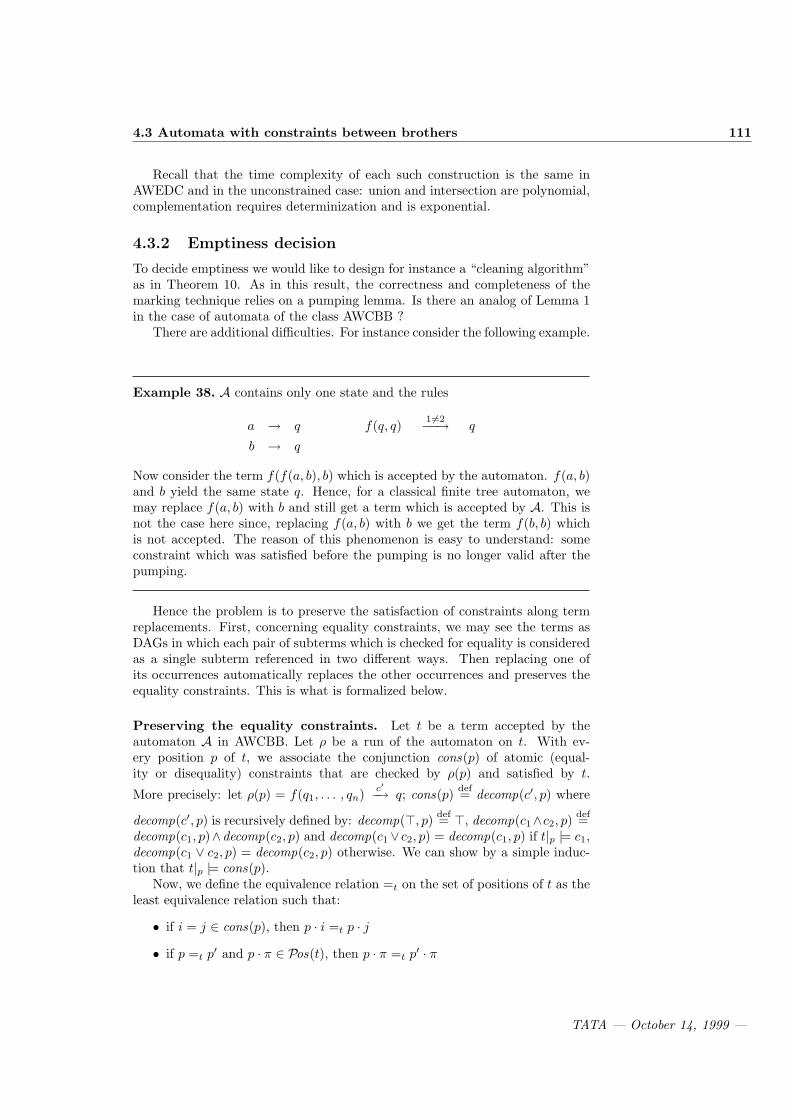
4.3 Automata with constraints between brothers 111
Recall that the time complexity of each such construction is the same inAWEDC and in the unconstrained case: union and intersection are polynomial,complementation requires determinization and is exponential.
4.3.2 Emptiness decision
To decide emptiness we would like to design for instance a “cleaning algorithm”as in Theorem 10. As in this result, the correctness and completeness of themarking technique relies on a pumping lemma. Is there an analog of Lemma 1in the case of automata of the class AWCBB ?
There are additional difficulties. For instance consider the following example.
Example 38. A contains only one state and the rules
a → q f(q, q)1 6=2−−→ q
b → q
Now consider the term f(f(a, b), b) which is accepted by the automaton. f(a, b)and b yield the same state q. Hence, for a classical finite tree automaton, wemay replace f(a, b) with b and still get a term which is accepted by A. This isnot the case here since, replacing f(a, b) with b we get the term f(b, b) whichis not accepted. The reason of this phenomenon is easy to understand: someconstraint which was satisfied before the pumping is no longer valid after thepumping.
Hence the problem is to preserve the satisfaction of constraints along termreplacements. First, concerning equality constraints, we may see the terms asDAGs in which each pair of subterms which is checked for equality is consideredas a single subterm referenced in two different ways. Then replacing one ofits occurrences automatically replaces the other occurrences and preserves theequality constraints. This is what is formalized below.
Preserving the equality constraints. Let t be a term accepted by theautomaton A in AWCBB. Let ρ be a run of the automaton on t. With ev-ery position p of t, we associate the conjunction cons(p) of atomic (equal-ity or disequality) constraints that are checked by ρ(p) and satisfied by t.
More precisely: let ρ(p) = f(q1, . . . , qn) c′−→ q; cons(p) def= decomp(c′, p) where
decomp(c′, p) is recursively defined by: decomp(>, p) def= >, decomp(c1∧c2, p) def=decomp(c1, p)∧decomp(c2, p) and decomp(c1∨ c2, p) = decomp(c1, p) if t|p |= c1,decomp(c1 ∨ c2, p) = decomp(c2, p) otherwise. We can show by a simple induc-tion that t|p |= cons(p).
Now, we define the equivalence relation =t on the set of positions of t as theleast equivalence relation such that:
• if i = j ∈ cons(p), then p · i =t p · j• if p =t p′ and p · π ∈ Pos(t), then p · π =t p′ · π
TATA — October 14, 1999 —

112 Automata with constraints
Note that in the last case, we have p′ · π ∈ Pos(t). Of course, if p =t p′, thent|p = t|p′ (but the converse is not necessarily true). Note also (and this is aproperty of the class AWCBB) that p =t p′ implies that the lengths of p and p′
are the same, hence, if p 6= p′, they are incomparable w.r.t. the prefix ordering.We can also derive from this remark that each equivalence class is finite (wemay assume that each equality constraint of the form i = i has been replacedby >).
Example 39. Consider the automaton whose transition rules are:
r1 : f(q, q) → q r2 : a → q
r3 : f(q, q) 1=2−−→ qf r4 : b → q
r5 : f(q, qf ) → qf r6 : f(qf , q) → qf
r7 : f(q, qf ) → q r8 : f(qf , q) → q
Let t = f(b, f(f(f(a, a), f(a, b)), f(f(a, a), f(a, b)))). A possible run of A on t isr5(r4, r3(r1(r1(r2, r2), r1(r2, r5)), r8(r3(r2, r2), r1(r2, r5)))) Equivalence classesof positions are:
Λ, 1, 2, 21, 22, 211, 221, 212, 222,2111, 2211, 2112, 2212, 2121, 2221, 2122, 2222
Let us recall the principle of pumping, for finite bottom-up tree automata(see Chapter 1). When a ground term C[C ′[t]] (C and C ′ are two contexts)is such that t and C ′[t] are accepted in the same state by an NFTA A, thenevery term C[C ′n[t]] (n ≥ 0) is accepted by A in the same state as C[C ′[t]]. Inother words, any C[C ′n[t]] ∈ L(A) may be reduced by pumping it up to theterm C[t] ∈ L(A). We consider here a position p (corresponding to the termC ′[t]) and its equivalence class [[p]] modulo =t. The simultaneous replacementon [[p]] with t in u, written u[t][[p]], is defined as the term obtained by successivelyreplacing the subterm at position p′ with t for each position p′ ∈ [[p]]. Since anytwo positions in [[p]] are incomparable, the replacement order is irrelevant. Now,a pumping is a pair (C[C ′[t]]p, C[C ′n[t]][[p]]) where C ′[t] and t are accepted inthe same state.
Preserving the disequality constraints. We have seen on Example 38that, if t is accepted by the automaton, replacing one of its subterms, say u,with a term v accepted in the same state as u, does not necessary yield anaccepted term. However, the idea is now that, if we have sufficiently manysuch candidates v, at least one of the replacements will keep the satisfaction ofdisequality constraints.
This is the what shows the following lemma which states that minimal ac-cepted terms cannot contain too many subterms accepted in the same state.
Lemma 5. Given any total simplification ordering, a minimal term acceptedby a deterministic automaton in AWCBB contains at most |Q| × N distinctsubterms where N is the maximal arity of a function symbol and |Q| is thenumber of states of the automaton.
TATA — October 14, 1999 —

4.3 Automata with constraints between brothers 113
⇓ Replacement
pN+1
=
= · · · 6= · · · = · · · 6= · · ·
pN+1
=
= · · · 6= · · · = · · · 6= · · ·
Figure 4.3: Constructing a smaller term accepted by the automaton
Proof. If ρ is a run, let τρ be the mapping from positions to states such thatτρ(p) is the target state of ρ(p).
If t is accepted by the automaton (let ρ be a successful run on t) and containsat least 1 + |Q| ×N distinct subterms, then there are at least N + 1 positionsp1, . . . , pN+1 such that τρ(p1) = . . . = τρ(pN+1) and t|p1 , . . . , t|pN+1 are dis-tinct. Assume for instance that t|pN+1 is the largest term (in the given totalsimplification ordering) among t|p1 , . . . , t|pN+1 . We claim that one of the terms
videf= t[t|pi ][[pN+1]] (i ≤ N) is accepted by the automaton.For each i ≤ N , we may define unambiguously a tree ρi by: ρi = ρ[ρ|pi ][[pN+1]].First, note that, by determinacy, for each position p ∈ [[pN+1]], τρ(p) =
τρ(pN+1) = τρ(pi). To show that there is a ρi which is a run, it remains to finda ρi the constraints of which are satisfied. Equality constraints of any ρi aresatisfied, from the construction of the equivalence classes (details are left to thereader).
Concerning disequality constraints, we choose i in such a way that all sub-terms at brother positions of pN+1 are distinct from t|pi (this choice is possiblesince N is the maximal arity of a function symbol and there are N distinctcandidates). We get a replacement as depicted on Figure 4.3.
Let pN+1 = π · k where k ∈ N (π is the position immediately above pN+1).Every disequality in cons(π) is satisfied by choice of i. Moreover, if p′ ∈ [[pN+1]]and p′ = π′ ·k′ with k′ ∈ N, then every disequality in mathitcons(π′) is satisfiedsince vi|π = vi|π′ .
Hence we constructed a term which is smaller than t and which is acceptedby the automaton. This yields the lemma.
Theorem 30. Emptiness can be decided in polynomial time for deterministicautomata in AWCBB.
Proof. The basic idea is that, if we have enough distinct terms in states q1, . . . , qn,then the transition f(q1, . . . , qn) c−→ q is possible. Use a marking algorithm (as
TATA — October 14, 1999 —

114 Automata with constraints
in Theorem 3) and keep for each state the terms that are known to be acceptedin this state. It is sufficient to keep at most N terms in each state (N is themaximal arity of a function symbol) according to Lemma 5 and the determinacyhypothesis (terms in different states are distinct). More precisely, we use thefollowing algorithm:
input: AWCBB A = (Q,F , Qf , ∆)begin
– Marked is a mapping which associates each state with a set ofterms accepted in that state.
Set Marked to the function which maps each state to the ∅repeat
Set Marked(q) to Marked(q) ∪ twhere
f ∈ Fn, t1 ∈ Marked(q1), . . . , tn ∈ Marked(qn),f(q1, . . . , qn) c−→ q ∈ ∆,
t = f(t1, . . . , tn) and t |= c,|Marked(q)| ≤ N − 1,
until no term can be added to any Marked(q)output: true if, for every state qf ∈ Qf , Marked(qf ) = ∅.
end
Complexity. For non-deterministic automata, an exponential time algorithmis derived from Proposition 20 and Theorem 30. Actually, in the non-deterministiccase, the problem is EXPTIME-complete.
We may indeed reduce the following problem which is known to be EXPTIME-complete to non-emptiness decision for nondeterministic AWCBB.Instance n tree automata A1, . . . ,An over F .Answer “yes” iff the intersection the respective languages recognized by A1,. . . ,An is not empty.
We may assume without loss of generality that the states sets of A1, . . . ,An
(called respectively Q1, . . . ,Qn) are pairwise disjoint, and that every Ai has asingle final state called qf
i . We also assume that n = 2k for some integer k. Ifthis is not the case, let k be the smallest integer i such that n < 2i and letn′ = 2k. We consider a second instance of the above problem: A′1, . . . ,A′n′where
A′i = Ai for each i ≤ n.
A′i = (q,F , q, f(q, . . . , q) → q|f ∈ F) for each n < i ≤ n′.
Note that the tree automaton in the second case is universal, i.e. it acceptsevery term of T (F). Hence, the answer is “yes” for A′1, . . . ,A′n′ iff it is “yes”for A1, . . . ,An.
TATA — October 14, 1999 —

4.4 Reduction automata 115
Now, we add a single new binary symbol g to F , getting F ′, and considerthe following AWCBB A:
A = (n⋃
i=1
Qi ] q1, . . . , qn−1,F ′, q1,∆)
where q1, . . . ,q2n−1 are new states, and the transition of ∆ are:
every transition rule of A1, . . . ,An is a transition rule of A,
for each i < n2 , g(q2i, q2i+1)
1=2−−→ qi is a transition rule of A,
for each i, n2 ≤ i < n− 1, g(qf
2i, qf2i+1)
1=2−−→ qi is a transition rule of A.
Note that A is non-deterministic, even if every Ai is deterministic.We can show by induction on k (n = 2k) that the answer to the above
problem is “yes” iff the language recognized by A is not empty. Moreover, thesize of A si linear in the size of the initial problem and A is constructed in a timewhich is linear in his size. This proves the EXPTIME-hardness of emptinessdecision for AWCBB.
4.3.3 Applications
The main difference between AWCBB and NFTA is the non-closure of AWCBBunder projection and cylindrification. Actually, the shift from automata on treesto automata on tuples of trees cannot be extended to the class AWCBB.
As long as we are interested in automata recognizing sets of trees, all resultson NFTA (and all applications) can be extended to the class AWCBB (with anbigger complexity). For instance, Theorem 23 (sort constraints) can be extendedto interpretations of sorts as languages accepted by AWCBB. The Proposition 15(encompassment) can be easily generalized to the case of non-linear terms inwhich non-linearities only occur between brother positions, provided that wereplace NFTA with AWCBB. Theorem 24 can also be generalized to the re-ducibility theory with predicates ·£t where t is non-linear terms, provided thatnon-linearities in t only occur between brother positions.
However, we can no longer invoke an embedding into WSkS. The importantpoint is that this theory only requires the weak notion of recognizability ontuples (Rec×). Hence we do not need automata on tuples, but only tuplesof automata. As an example of application, we get a decision algorithm forground reducibility of a term t w.r.t. left hand sides l1, . . . , ln, provided thatall non-linearities in t, l1, . . . , ln occur at brother positions: simply compute theautomata Ai accepting the terms that encompass li and check that L(A) ⊆L(A1) ∪ . . . ∪ L(An).
Finally, the application on reduction strategies does not carry over the caseof non-linear terms because there really need automata on tuples.
4.4 Reduction automata
As we have seen above, the first-order theory of finitely many unary encom-passment predicates ·£t1 , . . . , ·£tn
(reducibility theory) is decidable when non-linearities in the terms ti are restricted to brother positions. What happens
TATA — October 14, 1999 —
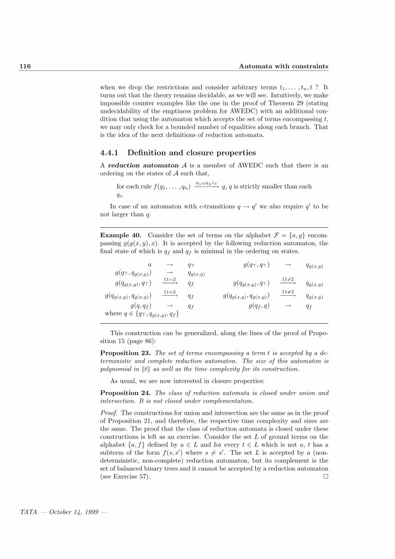
116 Automata with constraints
when we drop the restrictions and consider arbitrary terms t1, . . . , tn, t ? Itturns out that the theory remains decidable, as we will see. Intuitively, we makeimpossible counter examples like the one in the proof of Theorem 29 (statingundecidability of the emptiness problem for AWEDC) with an additional con-dition that using the automaton which accepts the set of terms encompassing t,we may only check for a bounded number of equalities along each branch. Thatis the idea of the next definitions of reduction automata.
4.4.1 Definition and closure properties
A reduction automaton A is a member of AWEDC such that there is anordering on the states of A such that,
for each rule f(q1, . . . , qn) π1=π2∧c−−−−−−→ q, q is strictly smaller than eachqi.
In case of an automaton with ε-transitions q → q′ we also require q′ to benot larger than q.
Example 40. Consider the set of terms on the alphabet F = a, g encom-passing g(g(x, y), x). It is accepted by the following reduction automaton, thefinal state of which is qf and qf is minimal in the ordering on states.
a → q> g(q>, q>) → qg(x,y)
g(q>, qg(x,y)) → qg(x,y)
g(qg(x,y), q>) 11=2−−−→ qf g(qg(x,y), q>)11 6=2−−−→ qg(x,y)
g(qg(x,y), qg(x,y))11=2−−−→ qf g(qg(x,y), qg(x,y))
11 6=2−−−→ qg(x,y)
g(q, qf ) → qf g(qf , q) → qf
where q ∈ q>, qg(x,y), qf
This construction can be generalized, along the lines of the proof of Propo-sition 15 (page 86):
Proposition 23. The set of terms encompassing a term t is accepted by a de-terministic and complete reduction automaton. The size of this automaton ispolynomial in ‖t‖ as well as the time complexity for its construction.
As usual, we are now interested in closure properties:
Proposition 24. The class of reduction automata is closed under union andintersection. It is not closed under complementation.
Proof. The constructions for union and intersection are the same as in the proofof Proposition 21, and therefore, the respective time complexity and sizes arethe same. The proof that the class of reduction automata is closed under theseconstructions is left as an exercise. Consider the set L of ground terms on thealphabet a, f defined by a ∈ L and for every t ∈ L which is not a, t has asubterm of the form f(s, s′) where s 6= s′. The set L is accepted by a (non-deterministic, non-complete) reduction automaton, but its complement is theset of balanced binary trees and it cannot be accepted by a reduction automaton(see Exercise 57).
TATA — October 14, 1999 —

4.4 Reduction automata 117
The weak point is of course the non-closure under complement. Conse-quently, this is not possible to reduce the non-determinism.
However, we have a weak version of stability:
Proposition 25. • With each reduction automaton, we can associate acomplete reduction automaton which accepts the same language. More-over, this construction preserves the determinism.
• The class of complete deterministic reduction automata is closed undercomplement.
4.4.2 Emptiness decision
Theorem 31. Emptiness is decidable for the class of reduction automata.
The proof of this result is quite complicated and gives quite high upperbounds on the complexity (a tower of several exponentials). Hence, we are notgoing to reproduce it here. Let us only sketch how it works, in the case ofdeterministic reduction automata.
As in Section 4.3.2, we have both to preserve equality and disequality con-straints.
Concerning equality constraints, we also define an equivalence relation be-tween positions (of equal subtrees). We cannot claim any longer that two equiv-alent positions do have the same length. However, some of the properties of theequivalence classes are preserved: first, they are all finite and their cardinalcan be bounded by a number which only depends on the automaton, becauseof the condition with the ordering on states (this is actually not true for theclass AWCBB). Then, we can compute a bound b2 (which only depends on theautomaton) such that the difference of the lengths of two equivalent positionsis smaller than b2. Nevertheless, as in Section 4.3.2, equalities are not a realproblem, as soon as the automaton is deterministic. Indeed, pumping can thenbe defined on equivalence classes of positions. If the automaton is not determin-istic, the problem is more difficult since we cannot guarantee that we reach thesame state at two equivalent positions, hence we have to restrict our attentionto some particular runs of the automaton.
Handling disequalities requires more care; the number of distinct subterms ofa minimal accepted term cannot be bounded as for AWCBB by |Q|×N , where Nis the maximal arity of a function symbol. The problem is the possible “overlap”of disequalities checked by the automaton. As in Example 38, a pumping mayyield a term which is no longer accepted, since a disequality checked somewherein the term is no longer satisfied. In such a case, we say that the pumping createsan equality. Then, we distinguish two kinds of equalities created by a pumping:the close equalities and the remote equalities. Roughly, an equality createdby a pumping (t[v(u)]p, t[u]p) is a pair of positions (π ·π1, π ·π2) of t[v(u)]p whichwas checked for disequality by the run ρ at position π on t[v(u)]p and such thatt[u]p|π·π1 = t[u]p|π·π2 (π is the longest common prefix to both members of thepair). This equality (π · π1, π · π2) is a close equality if π ≤ p < π · π1 orπ ≤ p < π · π2. Otherwise (p ≥ π · π1 or p ≥ π · π2), it is a remote equality. Thedifferent situations are depicted on Figures 4.4 and 4.5.
One possible proof sketch is
TATA — October 14, 1999 —

118 Automata with constraints
π π2π π1
π
p
π π2π π1
π
p
Figure 4.4: A close equality is created
π π2
π π1
π
pπ π2
π π1
π
p
Figure 4.5: A remote equality is created
TATA — October 14, 1999 —

4.4 Reduction automata 119
• First show that it is sufficient to consider equalities that are created atpositions around which the states are incomparable w.r.t. >
• Next, show that, for a deep enough path, there is at least one pumpingwhich does not yield a close equality (this makes use of a combinatorialargument; the bound is an exponential in the maximal size of a constraint).
• For remote equalities, pumping is not sufficient. However, if some pump-ing creates a remote equality anyway, this means that there are “big”equalterms in t. Then we switch to another branch of the tree, combining pump-ing in both subtrees to find one (again using a combinatorial argument)such that no equality is created.
Of course, this is a very sketchy proof. The reader is referred to the bibliog-raphy for more information about the proof.
4.4.3 Finiteness decision
The following result is quite difficult to establish. We only mention them forsake of completeness.
Theorem 32. Finiteness of the language is decidable for the class of reductionautomata.
4.4.4 Term rewriting systems
There is a strong relationship between reduction automata and term rewriting.We mention them readers interested in that topic.
Proposition 26. Given a term rewriting system R, the set of ground R-normalforms is recognizable by a reduction automaton, the size of which is exponentialin the size of R. The time complexity of the construction is exponential.
Proof. The set of R-reducible ground terms can be defined as the union of setsof ground terms encompassing the left members of rules of R. Thus, by Propo-sitions 23 and 24 the set of R-reducible ground terms is accepted by a deter-ministic and complete reduction automaton. For the union, we use the productconstruction, preserving determinism (see the proof of Theorem 5, Chapter 1)with the price of an exponential blowup. The set of ground R-normal formsis the complement of the set of ground R-reducible terms, and it is thereforeaccepted by a reduction automaton, according to Proposition 25.
Thus, we have the following consequence of Theorems 32 and 31.
Corollary 5. Emptiness and finiteness of the language of ground R-normalforms is decidable for every term rewriting system R.
Let us cite another important result concerning recognizability of sets normalforms.
Theorem 33. The membership of the language of ground normal forms to theclass of recognizable tree languages is decidable.
TATA — October 14, 1999 —
120 Automata with constraints
4.4.5 Application to the reducibility theory
Consider the reducibility theory of Section 3.4.2: there are unary predicate sym-bols ·£t which are interpreted as the set of terms which encompass t. However,we accept now non linear terms t as indices.
Propositions 23, and 24, and 25 yield the following result:
Theorem 34. The reducibility theory associated with any sets of terms is de-cidable.
And, as in the previous chapter, we have, as an immediate corollary:
Corollary 6. Ground reducibility is decidable.
4.5 Other decidable subclasses
Complexity issues and restricted classes. There are two classes of au-tomata with equality and disequality constraints for which tighter complexityresults are known:
• For the class of automata containing only disequality constraints, empti-ness can be decided in deterministic exponential time. For any termrewriting system R, the set of ground R-normal forms is still recogniz-able by an automaton of this subclass of reduction automata.
• For the class of deterministic reduction automata for which the constraints“cannot overlap”, emptiness can be decided in polynomial time.
Combination of AWCBB and reduction automata. If you relax thecondition on equality constraints in the transition rules of reduction automata soas to allow constraints between brothers, you obtain the biggest known subclassof AWEDC with a decidable emptiness problem.
Formally, these automata, called generalized reduction automata, aremembers of AWEDC such that there is an ordering on the states set such that,
for each rule f(q1, . . . , qn) π1=π2∧c−−−−−−→ q, q is a lower bound of q1, . . . , qnand moreover, if |π1| > 1 or |π2| > 1, then q is strictly smaller thaneach qi.
The closure and decidability results for reduction automata may be trans-posed to generalized reduction automata, with though a longer proof for theemptiness decision. Generalized reduction automata can thus be used for thedecision of reducibility theory extended by some restricted sort declarations. Inthis extension, additionally to encompassment predicates ·£t, we allow a familyof unary sort predicates . ∈ S, where S is a sort symbol. But, sort declarationsare limited to atoms of the form t ∈ S where where non linear variables in tonly occur at brother positions. This fragment is decidable by an analog ofTheorem 34 for generalized reduction automata.
TATA — October 14, 1999 —

4.6 Tree Automata with Arithmetic Constraints 121
4.6 Tree Automata with Arithmetic Constraints
Tree automata deal with finite trees which have a width bounded by the maxi-mal arity of the signature but there is no limitation on the depth of the trees.A natural idea is to relax the restriction on the width of terms by allowingfunction of variadic arity. This has been considered by several authors for ap-plications to graph theory, typing in object-oriented languages, temporal logicand automated deduction. In these applications, variadic functions are set ormultiset constructors in some sense, therefore they enjoy additional propertieslike associativity and/or commutativity and several types of tree automata havebeen designed for handling these properties. We describe here a class of treeautomata which recognize terms build with usual function symbols and multisetconstructors. Therefore, we deal not only with terms, but with so-called flatterms. Equality on these terms is no longer the syntactical identity, but it isextended by the equality of multisets under permutation of their elements. Torecognize sets of flat terms with automata, we shall use constrained rules wherethe constraints are Presburger’s arithmetic formulas which set conditions on themultiplicities of terms in multisets. These automata enjoy similar properties toNFTA and are used to test completeness of function definitions and inductivereducibility when associative-commutative functions are involved, provided thatsome syntactical restrictions hold.
4.6.1 Flat Trees
The set of function symbols G is composed of F , the set of function symbolsand of M, the set of function symbols for building multisets. For simplicity weshall assume that there is only one symbol of the latter form, denoted by t andwritten as an infix operator. The set of variables is denoted by X . Flat termsare terms generated by the non-terminal T of the following grammar.
N ::= 1 | 2 | 3 . . .T ::= S |U (flat terms)S ::= x | f(T1, . . . , Tn) (flat terms of sort F)U ::= N1.S1 t . . . tNp.Sp (flat terms of sort t)
where x ∈ X , n ≥ 0 is the arity of f , p ≥ 1 and∑i=p
i=1 Ni ≥ 2. Moreover theinequality ti 6=P tj holds for i 6= j, 1 ≤ i, j < n, where =P is defined as thesmallest congruence such that:
• x =P x,
• f(s1, . . . , sn) =P f(t1, . . . , tn) if f ∈ F and si =P ti for i = 1, . . . , n,
• n1.s1 t . . . t np.sp =P m1.t1 t . . . t mq.tq if p = q and there is somepermutation σ on 1, . . . , p such that si =P tσ(i) and ni = mσ(i) fori = 1, . . . , p.
Example 41. 3.a and 3.a t 2.f(x, b) are flat terms, but 2.a t 1.a t f(x, b) isnot since 2.a and 1.a must be grouped together to make 3.a.
TATA — October 14, 1999 —

122 Automata with constraints
The usual notions on terms can be generalized easily for flat terms. Werecall only what is needed in the following. A flat term is ground if it containsno variables. The root of a flat term is defined by
• for the flat terms of sort F , root(x) = x, root(f(t1, . . . , tn)) = f ,
• for the flat terms of sort t, root(s1 t . . . t sn) = t.
Our notion of subterm is slightly different from the usual one. We say thats is a subterm of t if and only if
• either s and t are identical,
• or t = f(s1, . . . , sn) and s is a subterm of some si,
• or t = n1.t1 t . . . t np.tp and s is a subterm of some ti.
For simplicity, we extend t to an operation between flat terms s, t denoting(any) flat term obtained by regrouping elements of sort F in s and t whichare equivalent modulo =P , leaving the other elements unchanged. For instances = 2.a t 1.f(a, a) and t = 3.b t 2.f(a, a) yields s t t = 2.a t 3.b t 3.f(a, a).
4.6.2 Automata with Arithmetic Constraints
There is some regularity in flat terms that is likely to be captured by some classof automata-like recognizers. For instance, the set of flat terms such that allinteger coefficients occurring in the terms are even, seems to be easily recogniz-able, since the predicate even(n) can be easily decided. The class of automatathat we describe now has been designed for accepting such sets of ground flatterms. A flat tree automaton with arithmetic constraints (NFTAC) overG is a tuple (QF , Qt,G, Qf , ∆) where
• QF ∪Qt is a finite set of states, such that
– QF is the set of states of sort F ,
– Qt is the set of states of sort t,
– QF ∩Qt = ∅,
• Qf ⊆ QF tQt is the set of final states,
• ∆ is a set of rules of the form:
– f(q1, . . . , qn) → q, for n ≥ 0, f ∈ Fn, q1, . . . , qn ∈ QF ∪ Qt, andq ∈ QF ,
– N.qc(N)−→ q′, where q ∈ QF , q′ ∈ Qt, and c is a Presburger’s arith-
metic2 formula with the unique free variable N ,
– q1 t q2 → q3 where q1, q2, q3 ∈ Qt.
Moreover we require that2Presburger’s arithmetic is first order arithmetic with addition and constants 0 and 1. This
fragment of arithmetic is known to be decidable.
TATA — October 14, 1999 —

4.6 Tree Automata with Arithmetic Constraints 123
– q1 t q2 → q3 is a rule of ∆ implies that q2 t q1 → q3 is also a rule of∆,
– q1 t (q2 t q3) → q4 is a rule of ∆ implies that (q1 t q2) t q3 → q4 isalso a rule of ∆ where q2tq3 (resp. q1tq2) denotes any state q′ suchthat there is a rule q2 t q3 → q′ (resp. q1 t q2 → q′).
These two conditions on ∆ will ensure that two flat terms equivalent modulo=P reach the same states.
Example 42. Let F = a, f and let A = (QF , Qt,G, Qf ,∆) where
QF = q, Qt = qt,Qf = qu,
∆ =
a −→ q N.q
∃n:N=2n−→ qtf( , ) −→ q qt t qt −→ qt
where stands for q or qt.
Let A = (QF , Qt,G, Qf , ∆) be a flat tree automaton. The move relation→A is defined by: let t, t′ ∈ T (F ∪Q,X), then t→A t′ if and only if there is acontext C ∈ C(G ∪Q) such that t = C[s] and t′ =P C[s′] where
• either there is some f(q1, . . . , qn) → q′ ∈ ∆ and s = f(q1, . . . , qn), s′ = q′,
• or there is some N.qc(N)−→ q′ ∈ ∆ and s = n.q with |= c(n), s′ = q′,
• or there is some q1 t q2 → q3 ∈ ∆ and s = q1 t q2, s′ = q3.
∗→A is the reflexive and transitive closure of →A.
Example 43. Using the automaton of the previous example, one has2.a t 6.f(a, a) t 2.f(a, 2.a) ∗→A 2.q t 6.f(q, q) t 2.f(q, 2.q)
∗→A 2.q t 6.q t 2.f(q, qt)∗→A 2.q t 6.q t 2.q∗→A qt t qt t qt
∗→A qt t qt∗→A qt
We define now semilinear flat languages. Let A = (QF , Qt,G, Qf , ∆) bea flat tree automaton. A ground flat term t is accepted by A, if there is someq ∈ Qf such that t
∗→A q. The flat tree language L(A) accepted by A is theset of all ground flat terms accepted by A. A set of flat terms is semilinear ifthere L = L(A) for some NFTAC A. Two flat tree automata are equivalent ifthey recognize the same language.
Example 44. The language of terms accepted by the automaton of Example 42is the set of ground flat terms with root t such that for each subterm n1.s1 t. . . t np.sp we have that ni is an even number.
TATA — October 14, 1999 —

124 Automata with constraints
Flat tree automata are designed to take into account the =P relation, whichis stated by the next proposition.
Proposition 27. Let s, t, be two flat terms such that s =P t, let A be a flattree automaton, then s
∗→A q implies t∗→A q.
Proof. The proof is by structural induction on s.
Proposition 28. Given a flat term t and a flat tree automaton A, it is decidablewhether t is accepted by A.
Proof. The decision algorithm for membership for flat tree automata is nearlythe same as the one for tree automata presented in Chapter 1, using an oraclefor the decision of Presburger’s arithmetic formulas.
Our definition of flat tree automata corresponds to nondeterministic flat treeautomata. We now define deterministic flat tree automata (DFTAC).
Let A = (QF , Qt,G, Qf , ∆) be a NFTAC over G.
• The automaton A is deterministic if for each ground flat term t, thereis at most one state q such that t
∗→A q.
• The automaton A is complete if for each ground flat term t, there a statesuch that t
∗→A q.
• A state q is accessible if there is one ground flat term t such that t∗→A q.
The automaton is reduced if all states are accessible.
4.6.3 Reducing non-determinism
As for usual tree automata, there is an algorithm for computing an equivalentDFTAC from any NFTAC which proves that a language recognized by a NFTACis also recognized by a DFTAC. The algorithm is similar to the determiniza-tion algorithm of the class AWEDC: the ambiguity arising from overlappingconstraints is lifted by considering mutually exclusive constraints which coverthe original constraints, and using sets of states allows to get rid of the non-determinism of rules having the same left-hand side. Here, we simply have todistinguish between states of QF and states of Qt.
Determinization algorithm
input A = (QF , Qt,G, Qf ,∆) a NFTAC.
begin
A state [q] of the equivalent DFTAC is in 2QF ∪ 2Qt .
Set QdF = ∅, Qd
t = ∅, ∆d = ∅.repeat
for each f of arity n, [q]1, . . . , [q]n ∈ QdF ∪Qd
t do
let [q] = q | ∃f(q1, . . . , qn) → q ∈ ∆ with qi ∈ [q]i for i = 1, . . . , n
TATA — October 14, 1999 —

4.6 Tree Automata with Arithmetic Constraints 125
in Set QdF to Qd
F ∪ [q]Set ∆d to ∆d ∪ f([q]1, . . . , [q]n) → [q]
endfor
for each [q] ∈ QF do
for each [q′] ⊆ q′′ | ∃N.qc(N)−→ q′′ ∈ ∆ with q ∈ [q] do
let C be( ∧
q∈[q]
∨
N.qci(N)−→ q′′∈∆
q′′∈[q′]
ci(N))∧
( ∧
q/∈[q]
∧
N.qci(N)−→ q′′∈∆
q′′∈[q′]
¬ci(N))
in Set Qdt to Qd
F ∪ [q′]Set ∆d to ∆d ∪ N.[q]
C(N)−→ [q′]
endfor
endfor
for each [q]1, [q]2 ∈ Qdt do
let [q] = q | ∃q1 ∈ [q]1, q2 ∈ [q]2, q1 t q2 → q3 ∈ ∆in Set Qd
t to QdF ∪ [q]
Set ∆d to ∆d ∪ [q]1 t [q]2 → [q]endfor
until no rule can be added to ∆d
Set Qdf = [q] ∈ Qd
F ∪Qdt | [q] ∩Qf 6= ∅,
end
output: Ad = (QdF , Qd
t,F , Qdf , ∆d)
Proposition 29. The previous algorithm terminates and computes a determin-istic flat tree automaton equivalent to the initial one.
Proof. The termination is obvious. The proof of the correctness relies on thefollowing lemma:
Lemma 6. t∗→Ad
[q] if and only if t∗→A q for all q ∈ [q].
The proof is by structural induction on t and follows the same pattern asthe proof for the class AWEDC.
Therefore we have proved the following theorem stating the equivalence be-tween DFTAC and NFTAC.
Theorem 35. Let L be a semilinear set of flat terms, then there exists a DF-TAC that accepts L.
TATA — October 14, 1999 —

126 Automata with constraints
4.6.4 Closure Properties of Semilinear Flat Languages
Given an automaton A = (Q,G, Qf , ∆), it is easy to construct a equivalentcomplete automaton. If A is not complete then
• add two new trash states qt of sort F and qtt of sort t,
• for each f ∈ F , q1, . . . , qn ∈ Q∪qt, qtt , such that there is no rule having
f(q1, . . . , qn) as left-hand side, then add f(q1, . . . , qn) → qt,
• for each q of sort F , let c1(N), . . . , cm(N) be the conditions of the rules
N.qci(N)−→ q′,
– if the formula ∃N (c1(N) ∨ . . . ∨ cm(N)) is not equivalent to true,
then add the rule N.q¬(c1(N)∨...∨cm(N))(N)−→ qtt ,
– if there are some q, q′ of sort t such that there is no rule qt q′ → q”,then add the rules q t q′ → qtt and q′ t q → qtt .
– if there is some rule (q1 t q2) t q3 → qtt (resp. q1 t (q2 t q3) → qtt ,add the rule q1 t (q2 t q3) → qtt (resp. (q1 t q2) t q3 → qtt ) if it ismissing.
This last step ensures that we build a flat tree automaton, and it is straight-forward to see that this automaton is equivalent to the initial one (same proofas for DFTA). This is stated by the following proposition.
Theorem 36. For each flat tree automaton A, there exists a complete equiva-lent automaton B.
Example 45. The automaton of Example 42 is not complete. It can becompleted by adding the states qt, q
tt , and the rules N.qt
N≥0−→ qttN.q
∃n N=2n+1−→ qttf( , ) −→ qt
where ( , ) stands for a pair of q, qt, qt, qtt such that if a rule the left hand side
of which is f( , ) is not already in ∆.
Theorem 37. The class of semilinear flat languages is closed under union.
Proof. Let L (resp. M) be a semilinear flat language recognized by A =(QF , Qt,G, Qf ,∆) (resp. B = (Q′
F , Q′t,G, Q′
f , ∆′)), then L ∪M is recognizedby C = (QF ∪Q′F , Qt ∪Q′
t,G, Qf ∪Q′f , ∆ ∪∆′).
Theorem 38. The class of semilinear flat languages is closed under comple-mentation.
Proof. Let A be an automaton recognizing L. Compute a complete automatonB equivalent to A. Compute a deterministic automaton C equivalent to B usingthe determinization algorithm. The automaton C is still complete, and we get anautomaton recognizing the complement of L by exchanging final and non-finalstates in C.
TATA — October 14, 1999 —

4.6 Tree Automata with Arithmetic Constraints 127
¿From the closure under union and complement, we get the closure underintersection (a direct construction of an automaton recognizing the intersectionalso exists).
Theorem 39. The class of semilinear flat languages is closed under intersec-tion.
4.6.5 Emptiness Decision
The last important property to state is that the emptiness of the languagerecognized by a flat tree automaton is decidable. The decision procedure relieson an algorithm similar to the decision procedure for tree automata combinedto a decision procedure for Presburger’s arithmetic. However a straightforwardmodification of the algorithm in Chapter 1 doesn’t work. Assume that theautomaton contains the rule qt1 t qt1 → qt2 and assume that there is some flat
term t such that 1.t∗
→A qt1 . ¿From these two hypothesis, we can not infer that1.t t 1.t
∗→A qt2 since 1.t t 1.t is not a flat term, contrary to 2.t. Thereforethe decision procedure involves some combinatorics in order to ensure that wealways deal with correct flat terms.
¿From now on, let A = (QF , Qt,G, Qf ,∆) be some given deterministic flattree automaton and let M be the number of states of sort t. First, we need tocontrol the possible infinite number of solutions of Presburger’s conditions.
Proposition 30. There is some computable B such that for each conditionc(N) of the rules of A, either each integer n validating c is smaller than B orthere are at least M + 1 integers smaller than B validating c.
Proof. First, for each constraint c(N) of a rule of ∆, we check if c(N) has afinite number of solutions by deciding if ∃P : c(N) ⇒ N < P is true. If c(N)has a finite number of solutions, it is easy to find a bound B1(c(N)) on thesesolutions by testing ∃n : n > k ∧ c(n) for k = 1, 2, . . . until it is false. If c(N)has an infinite number of solutions, one computes the Mth solution obtainedby checking |= c(k) for k = 1, 2, . . . . We call this Mth solution B2(c(N)). Thebound B is the maximum of all the B1(c(N))’s and B2(c(N))’s.
Now we control the maximal width of terms needed to reach a state.
Proposition 31. For all t∗→A q, there is some s
∗→A q such that for each sub-term of s of the form n1.v1 t . . . t np.vp, we have p ≤ M and ni ≤ B.
Proof. The bound on the coefficients ni is a direct consequence of the previousproposition. The proof on p is by structural induction on t. The only non-trivialcase is for t = m1.t1 t . . . tmk.tk. Let us assume that t is the term with thesmallest value of k among the terms t′ | t′ ∗→A q.
First we show that k ≤ M . Let qti be the states such that ni.ti→A qti .We have thus t
∗→A qt1 t . . . t qtk∗→A q. By definition of DFTAC, the reduction
qt1 t . . . t qtk∗→A q has the form:
qt1 t . . . t qtk∗→A
qt[12] t qt3 t . . . t qtk∗→A
. . .∗→A
qt[1...k] = q
for some states qt[12], . . . , qt[1...k] of Qt.
TATA — October 14, 1999 —
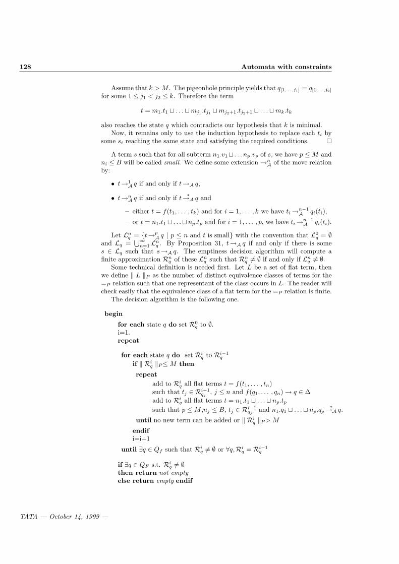
128 Automata with constraints
Assume that k > M . The pigeonhole principle yields that q[1,... ,j1] = q[1,... ,j2]
for some 1 ≤ j1 < j2 ≤ k. Therefore the term
t = m1.t1 t . . . tmj1 .tj1 tmj2+1.tj2+1 t . . . tmk.tk
also reaches the state q which contradicts our hypothesis that k is minimal.Now, it remains only to use the induction hypothesis to replace each ti by
some si reaching the same state and satisfying the required conditions.
A term s such that for all subterm n1.v1t . . . np.vp of s, we have p ≤ M andni ≤ B will be called small. We define some extension →n
A of the move relationby:
• t→1A q if and only if t→A q,
• t→nA q if and only if t
∗→A q and
– either t = f(t1, . . . , tk) and for i = 1, . . . , k we have ti→n−1A qi(ti),
– or t = n1.t1 t . . .t np.tp and for i = 1, . . . , p, we have ti→n−1A qi(ti).
Let Lnq = t→p
A q | p ≤ n and t is small with the convention that L0q = ∅
and Lq =⋃∞
n=1 Lnq . By Proposition 31, t→A q if and only if there is some
s ∈ Lq such that s→A q. The emptiness decision algorithm will compute afinite approximation Rn
q of these Lnq such that Rn
q 6= ∅ if and only if Lnq 6= ∅.
Some technical definition is needed first. Let L be a set of flat term, thenwe define ‖ L ‖P as the number of distinct equivalence classes of terms for the=P relation such that one representant of the class occurs in L. The reader willcheck easily that the equivalence class of a flat term for the =P relation is finite.
The decision algorithm is the following one.
begin
for each state q do set R0q to ∅.
i=1.repeat
for each state q do set Riq to Ri−1
q
if ‖ Riq ‖P≤ M then
repeatadd to Ri
q all flat terms t = f(t1, . . . , tn)such that tj ∈ Ri−1
qj, j ≤ n and f(q1, . . . , qn) → q ∈ ∆
add to Riq all flat terms t = n1.t1 t . . . t np.tp
such that p ≤ M ,nj ≤ B, tj ∈ Ri−1qj
and n1.q1 t . . . t np.qp∗→A q.
until no new term can be added or ‖ Riq ‖P > M
endifi=i+1
until ∃q ∈ Qf such that Riq 6= ∅ or ∀q,Ri
q = Ri−1q
if ∃q ∈ QF s.t. Riq 6= ∅
then return not emptyelse return empty endif
TATA — October 14, 1999 —

4.6 Tree Automata with Arithmetic Constraints 129
end
Proposition 32. The algorithm terminates after n iterations for some n andRn
q = ∅ if and only if Lq = ∅
Proof. At every iteration, either one Riq increases or else all the Ri
q’s are leftuntouched in the repeat . . . until loop. Therefore the termination conditionwill be satisfied after a finite number of iterations, since equivalence classes for=P are finite.
By construction we have Rmq ⊆ Lm
q , but we need the following additionalproperty.
Lemma 7. For all m,Rmq = Lm
q or Rmq ⊆ Lm
q and ‖ Rmq ‖P > M
The proof is by induction on m.
Base case m = 0. Obvious from the definitions.
Induction step. We assume that the property is true for m and we prove thatit holds for m + 1.Either Lm
q = ∅ therefore Rmq = ∅ and we are done, or Lm
q 6= ∅, which we assumefrom now on.
• q ∈ QF .
– Either there is some rule f(q1, . . . , qn) → q such that Rmqi6= ∅ for
all i = 1, . . . , n and such that for some q′ among q1, . . . , qn, wehave ‖ Rm
q′ ‖P > M . Then we can construct at least M + 1 termst = f(t1, . . . , t′, . . . , tn) where t′ ∈ Rm
q′ , such that t ∈ Rm+1q by
giving M + 1 non equivalent values to t′ (corresponding values for tare also non equivalent). This yields that ‖ Rm+1
q ‖P > M .
– Or there is no rule as above, therefore Rm+1q = Lm+1
q .
• q ∈ Qt.
For each small term t = n1.t1 t . . . t np.tp such that t ∈ Lm+1q , there
are some terms s1, . . . , sn in Rmqi
such that ti∗→A qi implies that si
∗→A qi.What we must prove is that ‖ Rm
qi‖P > M for some i ≤ p implies ‖
Rm+1q ‖P > M . Since A is deterministic, we have that s
∗→A q and t∗→A q′
with q 6= q′ implies that s 6=P t. Let S be the set of states occurring inthe sequence q1, . . . , qp. We prove by induction on the cardinal of S thatif there is some qi such that ‖ Rm
qi‖P > M , we can build at least M + 1
terms in Rm+1q otherwise we build at least one term of Rm+1
q .
Base case S = q′, and therefore all the qi are equal to q′. Either‖ Rm
q′ ‖P≤ M and we are done or ‖ Rmq′ ‖P > M and we know that there
are s1, . . . , sM+1, . . . pairwise non equivalent terms reaching q′. Therefore,there are at least
(M+1M
) ≥ M + 1 different non equivalent possible termsni1 .si1 t . . . t nip .sip . Moreover each of these terms S satisfies s→m+1
A q,which proves the result.
TATA — October 14, 1999 —

130 Automata with constraints
Induction step. Let S = S′ ∪ q′ where the property is true for S′. Wecan assume that ‖ Rm
q′ ‖P≤ M (otherwise all ‖ Rmqi‖P are less than or
equal to M ).
Let i1, . . . , ik be the positions of q′ in q1, . . . , qp, let j1, . . . , jl be the posi-tions of the states different from q′ in q1, . . . , qp. By induction hypothesis,there are some flat terms sj such that nj1 .sj1 t . . . t njl
.sjlis a valid flat
term. Since A is deterministic and q′ is different from all element of S′,we know that si 6=P sj for any i ∈ i1, . . . , ik, j ∈ j1, . . . , jk. There-fore, we use the same reasoning as in the previous case to build at leastCk
M+1 ≥ M + 1 pairwise non equivalent flat terms s = n1.s1 t . . . t np.sp
such that s→m+1A q.
The termination of the algorithm implies that for each m ≥ n, Rmq = Lm
q orRm
q ⊆ Lmq and ‖ Rm
q ‖P > M . Therefore Lq = ∅ if and only if Rnq = ∅.
The following theorem summarizes the previous results.
Theorem 40. Let A be a DFTAC, then it is decidable whether the languageaccepted by A is empty or not.
The reader should see that the property that A deterministic is crucial inproving the emptiness decision property. Therefore proving the emptiness of thelanguage recognized by a NFTAC implies to compute an equivalent DFTACfirst.
Another point is that the previous algorithm can be easily modified to com-pute the set of accessible states of A.
4.7 Exercises
Exercise 53.
1. Show that the automaton A+ of Example 35 accepts only terms of the formf(t1, s
n(0), sm(0), sn+m(0))
2. Conversely, show that, for every pair of natural numbers (n, m), there exists aterm t1 such that f(t1, s
n(0), sm(0), sn+m(0)) is accepted by A+.
3. Construct an automaton A× of the class AWEDC which has the same propertiesas above, replacing + with ×
4. Give a proof that emptiness is undecidable for the class AWEDC, reducingHilbert’s tenth problem.
Exercise 54. Give an automaton of the class AWCBB which accepts the set of terms
t (over the alphabet a(0), b(0), f(2)) having a subterm of the form f(u, u). (i.e the
set of terms that are reducible by a rule f(x, x) → v).
Exercise 55. Show that the class AWCBB is not closed under linear tree homomor-
phisms. Is it closed under inverse image of such morphisms ?
Exercise 56. Give an example of two automata in AWCBB such that the set of pairs
of terms recognized respectively by the automata is not itself a member of AWCBB.
TATA — October 14, 1999 —

4.7 Exercises 131
Exercise 57. (Proposition 24) Show that the class of (languages recognized by)
reduction automata is closed under intersection and union. Show that the set of bal-
anced term on alphabet a, f is not recognizable by a reduction automaton, showing
that the class of languages recognized by) reduction automata is not closed under
complement.
Exercise 58. Show that the class of languages recognized by reduction automata is
preserved under linear tree homomorphisms. Show however that this is no longer true
for arbitrary tree homomorphisms.
Exercise 59. Let A be a reduction automaton. We define a ternary relation qw−→ q′
contained in Q× N∗ ×Q as follows:
• for i ∈ N, qi−→ q′ if and only if there is a rule f(q1, . . . , qn)
c−→A
q′ with qi = q
• qi·w−−→ q′ if and only if there is a state q′′ such that q
i−→ q′′ and q′′w−→ q′.
Moreover, we say that a state q ∈ Q is a constrained state if there is a rule f(q1, . . . , qn)c−→A
q
in A such that c is not a valid constraint.We say that the the constraints of A cannot overlap if, for each rule f(q1, . . . , qn)
c−→ q
and for each equality (resp. disequality) π = π′ of c, there is no strict prefix p of π
and no constrained state q′ such that q′p−→ q.
1. Consider the rewrite system on the alphabet f(2), g(1), a(0) whose left mem-bers are f(x, g(x)), g(g(x)), f(a, a). Compute a reduction automaton, whoseconstraints do not overlap and which accepts the set of irreducible ground terms.
2. Show that emptiness can be decided in polynomial time for reduction automatawhose constraints do not overlap. (Hint: it is similar to the proof of Theorem30.)
3. Show that any language recognized by a reduction automaton whose constraintsdo not overlap is an homomorphic image of a language in the class AWCBB.Give an example showing that the converse is false.
Exercise 60. Prove the Proposition ?? along the lines of Proposition 15.
Exercise 61. The purpose of this exercise is to give a construction of an automatonwith disequality constraints (no equality constraints) whose emptiness is equivalent tothe ground reducibility of a given term t with respect to a given term rewriting systemR.
1. Give a direct construction of an automaton with disequality constraints ANF(R)
which accepts the set of irreducible ground terms
2. Show that the class of languages recognized by automata with disequality con-straints is closed under intersection. Hence the set of irreducible ground in-stances of a linear term is recognized by an automaton with disequality con-straints.
3. LetANF(R) = (QNF,F , QfNF, ∆NF). We computeANF,t
def= (QNF,t,F , Qf
NF,t, ∆NF,t)as follows:
• QNF,tdef= tσ|p | p ∈ Pos(t)×QNF where σ ranges over substitutions from
NLV (t) (the set of variables occurring at least twice in t) into QfNF.
• For all f(q1, . . . , qn)c−→ q ∈ ∆NF, and all u1, . . . , un ∈ tσ|p | p ∈ Pos(t),
∆NF,t contains the following rules:
TATA — October 14, 1999 —

132 Automata with constraints
– f([qu1 , q1], . . . , [qun , qn])c∧c′−−−→ [qf(u1,... ,un), q] if f(u1, . . . , un) = tσ0
and c′ is constructed as sketched below.
– f([qu1 , q1], . . . , [qun , qn])c−→ [qf(u1,... ,un), q] if [qf(u1,... ,un), q] ∈ QNF,t
and we are not in the first case.
– f([qu1 , q1], . . . , [qun , qn])c−→ [qq, q] in all other cases
c′ is constructed as follows. From f(u1, . . . , un) we can retrieve the rules appliedat position p in t. Assume that the rule at p checks π1 6= π2. This amounts tocheck pπ1 6= pπ2 at the root position of t. Let D be all disequalities pπ1 6= pπ2
obtained in this way. The non linearity of t implies some equalities: let E bethe set of equalities p1 = p2, for all positions p1, p2 such that t|p1 = t|p2 is avariable. Now, c′ is the set of disequalities π 6= π′ which are not in D and thatcan be inferred from D, E using the rules
pp1 6= p2, p = p′ ` p′p1 6= p2
p 6= p′, pp1 = p2 ` p′p1 6= p2
For instance, let t = f(x, f(x, y)) and assume that the automaton ANF con-
tains a rule f(q, q)16=2−−→ q. Then the automaton ANF,t will contain the rule
f([qq, q], [qf(q,q), q])16=2∧16=22−−−−−−−→ q.
The final states are [qu, qf ] where qf ∈ QfNF and u is an instance of t.
Prove that ANF,t accepts at least one term if and only if t is not ground reducibleby R.
Exercise 62. Prove Theorem 34 along the lines of the proof of Theorem 24.
Exercise 63. Show that the algorithm for deciding emptiness of deterministic com-
plete flat tree automaton works for non-deterministic flat tree automata such that for
each state q the number of non-equivalent terms reaching q is 0 or greater than or
equal to 2.
Exercise 64. (Feature tree automata)Let F be a finite set of feature symbols (or attributes) denoted by f, g, . . . and S bea set of constructor symbols (or sorts) denoted by A, B, . . . . In this exercise and thenext one, a tree is a rooted directed acyclic graph, a multitree is a tree such that thenodes are labeled over S and the edges over F . A multitree is either (A, ∅) or (A, E)where E is a finite multiset of pairs (f, t) with f a feature and t a multitree. A featuretree is a multitree such that the edges outgoing from the same node are labeled bydifferent features. The + operation takes a multitree t = (A, E), a feature f and amultitree t′ to build the multitree (A, E ∪ (f, t′)) denoted by t + ft′.
1. Show that t + f1t1 + f2t2 = t + f2t2 + f1t1 (OI axiom: order independenceaxiom) and that the algebra of multitrees is isomorphic to the quotient of thefree term algebra over + ∪ F ∪ S by OI.
2. A deterministic M-automaton is a triple (A, h, Qf ) where A is an finite + ∪F ∪S-algebra, h : M→A is a homomorphism, Qf (the final states) is a subsetof the set of the values of sort M. A tree is accepted if and only if h(t) ∈ Qf .
(a) Show that a M-automaton can be identified with a bottom-up tree au-tomaton such that all trees equivalent under OI reach the same states.
(b) A feature tree automaton is a M-automaton such that for each sort s (Mor F), for each q the set of the c’s of arity 0 interpreted as q in A is finiteor co-finite. Give a feature tree to recognize the set of natural numberswhere n is encoded as (0, suc, (0, . . . , (0, ∅))) with n edges labeled bysuc.
TATA — October 14, 1999 —

4.8 Bibliographic notes 133
(c) Show that the class of languages accepted by feature tree automata isclosed under boolean operations and that the emptiness of a languageaccepted by a feature automaton is decidable.
(d) A non-deterministic feature tree automaton is a tuple (Q, P, h, Qf ) suchthat Q is the set of states of sort M, P the set of states of sort F , h iscomposed of three functions h1 : S → 2Q, h2 : F → 2P and the transitionfunction + : Q×P ×Q → 2Q. Moreover q + p1q1 + p2q2 = q + p2q2 + p1q1
for each q, q1, q2, p1, p2, s ∈ S | p ∈ h1(s) and f ∈ F | p ∈ h2(f) arefinite or co-finite for each p. Show that any non-deterministic feature treeautomaton is equivalent to a deterministic feature tree automaton.
Exercise 65. (Characterization of recognizable flat feature languages)A flat feature tree is a feature tree of depth 1 where depth is defined by depth((A, ∅)) =0 and depth((A, E)) = 1+maxdepth(t) | (f, t) ∈ E. Counting constraints are definedby: C(x) ::= card(ϕ ∈ F | ∃y.(xϕy) ∧ Ty) = n mod m
| Sx| C(x) ∨ C(x)| C(x) ∧ C(x)
where n, m are integers, S and T finite or co-finite subsets of S, F a finite or co-finitesubset of F and n mod 0 is defined as n. The semantics of the first type of constraintis: C(x) holds if the number of edges of x going from the root to a node labeled by asymbol of T is equal to n mod m. The semantics of Sx is: Sx holds if the root of x islabeled by a symbol of S.
1. Show that the constraints are closed under negation. Show that the followingconstraints can be expressed in the constraint language (F is a finite subset ofF , f ∈ F , A ∈ S): there is one edge labeled f from the root, a given finitesubset of F . There is no edge labeled f from the root, the root is labeled by A.
2. A set L of flat multitrees is counting definable if and only if there some countingconstraint C such that L = x | C(x) holds. Show that a set of flat feature treesis counting definable if and only if it is recognizable by a feature tree automaton.hint: identify flat trees with multisets over (F ∪root)×S and + with multisetunion.
4.8 Bibliographic notes
RATEG appeared in Mongy’s thesis [Mon81]. Unfortunately, as shown in[Mon81] the emptiness problem is undecidable for the class RATEG (and hencefor AWEDC). The undecidability can be even shown for a more restricted classof automata with equality tests between cousins (see [Tom92]).The remarkable subclass AWCBB is defined in [BT92]. This paper presents theresults cited in section 4.3, especially theorem 30.Concerning complexity, the result used in section 4.3.2 (EXPTIME-completenessof the emptiness of the intersection of n recognizable tree languages) may befound in [FSVY91, Sei94b].[DCC95] is concerned with reduction automata and their use as a tool for thedecision of the encompassment theory in the general case.The first decidability proof for ground reducibility is due to [Pla85]. In [?],ground reducibility decision is shown EXPTIME-complete. In this work, anEXPTIME algorithm for emptiness decision for AWEDC with only disequalityconstrained The result mentioned in section 4.5.
TATA — October 14, 1999 —

134 Automata with constraints
The class of generalized reduction automata is introduced in [CCC+94]. In thispaper, a efficient cleaning algorithm is given for emptiness decision.
There have been many work dealing with automata where the width ofterms is not bounded. In [Cou89], Courcelle devises an algebraic notion of rec-ognizability and studies the case of equational theories. Then he gives severalequational theories corresponding to several notions of trees like ordered or un-ordered, ranked or unranked trees and provides the tree automata to acceptthese objects. Actually the axioms used for defining these notions are commu-tativity (for unordered) or associativity (for unranked) and what is needed is tobuild tree automata such that all element of the same equivalence class reachthe same state. Trees can be also defined as finite, acyclic rooted ordered graphsof bounded degree. Courcelle [Cou92] has devised a notion of of recognizableset of graphs and suggests to devise graph automata for accepting recognizablegraphs of bounded tree width. He gives such automata for trees defined as un-bounded, unordered, undirected, unrooted trees (therefore these are not whatwe call tree in this book). Actually, he shows that recognizable sets of graphsare (homomorphic image of) sets of equivalence class of terms, where the equiv-alence relation is the congruence induced by a set of equational axioms includingassociativity-commutativity axiom and identity element. He gives several equiv-alent notions for recognizability from which he gets the definitions of automatafor accepting recognizable languages.
Feature tree are a generalization of first-order trees introduced for modelingrecord structures. A feature tree is a finite tree whose nodes are labelled byconstructor symbols and edges are labelled by feature symbols Niehren andPodelski [NP93] have studied the algebraic structures of feature trees and havedevised feature tree automata for recognizing sets of feature trees. They haveshown that this class of feature trees enjoy the same properties as regular treelanguage and give a characterization of these sets using counting constraintswhich are a subset of Presburger’s arithmetic formulas. See exercise 64 for moredetails.
TATA — October 14, 1999 —

Chapter 5
Tree Set Automata
5.1 Introduction
“The notion of type expresses the fact that one just cannot apply any operatorto any value. Inferring and checking a program’s type is then a proof of partialcorrection” quoting Marie-Claude Gaudel. “The main problem in this field is tobe flexible while remaining rigorous, that is to allow polymorphism (a value canhave more than one type) in order to avoid repetitions and write very generalprograms while preserving decidability of their correction with respect to types.”
On that score, the set constraints formalism is a compromise between powerof expression and decidability. This has been the object of active research for afew years.
Set constraints are relations between sets of terms. For instance, let us definethe natural numbers with 0 and the successor relation denoted by s. Thus, theconstraint
Nat = 0 ∪ s(Nat) (5.1)
corresponds to this definition. Let us consider the following system:
Nat = 0 ∪ s(Nat)List = cons(Nat, List) ∪ nil
List+ ⊆ Listcar(List+) ⊆ s(Nat)
(5.2)
The first constraint defines natural numbers. The second constraint codes theset of LISP-like lists of natural numbers. The empty list is nil and other listsare obtained the constructor symbol cons. The last two constraints representthe set of lists with a non zero first element.
Set constraints are the essence of Set Based Analysis. The basic idea is toreason about program variables as sets of possible values. Set Based Analy-sis involves first writing set constraints expressing relationships between sets ofprogram values, and then solving the system of set constraints. A single approxi-mation is: all dependencies between the values of program variables are ignored.Techniques developed for Set Based Analysis have been successfully applied inprogram analysis and type inference and the technique can be combined withothers [HJ92].
TATA — October 14, 1999 —

136 Tree Set Automata
Set constraints have also been used to define a constraint logic programminglanguage over sets of ground terms that generalizes ordinary logic programmingover an Herbrand domain [Koz94].
In a more general way, a system of set constraints is a conjunction of positiveconstraints of the form exp ⊆ exp′1 and negative constraints of the form exp 6⊆exp′. Right hand side and left hand side of these inequalities are set expressions,which are built with
• function symbols: in our example 0, s, cons, nil are function symbols.
• operators: union ∪, intersection ∩, complement ∼
• projection symbols: for instance, in the last equation of system (5.2) cardenotes the first component of cons. In the set constraints syntax, this iswritten cons−1
(1).
• set variables like Nat or List.
An interpretation assigns to each set variable a set of terms only built withfunction symbols. A solution is an interpretation which satisfies the system.For example, 0, s(0), s(s(0)), . . . is a solution of Equation (5.1).
In the set constraint formalism, set inclusion and set union express in anatural way parametric polymorphism: List ⊆ nil ∪ cons(X, List).
In logic or functional programming, one often use dynamic procedures todeal with type. In other words, a run-time procedure checks whether or not anexpression is well-typed. This permits maximum programming flexibility at thepotential cost of efficiency and security. Static analysis partially avoids thesedrawbacks with the help of type inference and type checking procedures. Theinformation extracted at compile time is also used for optimization.
Basically, program sources are analyzed at compile time and an ad hoc for-malism is used to represent the result of the analysis. For types considered assets of values, the set constraints formalism is well suited to represent them andto express their relations. Numerous inference and type checking algorithms inlogic, functional and imperative programming are based on a resolution proce-dure for set constraints.
Most of the earliest algorithms consider systems of set constraints with weakpower of expression. More often than not, these set constraints always have aleast solution — w.r.t. inclusion — which corresponds to a (tuple of) regularset of terms. In this case, types are usual sorts. A sort signature defines atree automaton (see Section 3.4.1 for the correspondence between automataand sorts). Therefore, these methods are closely related finite tree automataand use classical algorithms on these recognizers, like the ones presented inChapter 1.
In order to obtain a more precise information, it is necessary to enrich theset constraints vocabulary. In one hand, with a large vocabulary an analysis
1exp = exp′ for exp ⊆ exp′ ∧ exp′ ⊆ exp.
TATA — October 14, 1999 —

5.1 Introduction 137
can be accurate and relevant, but on the other hand, solutions are difficult toobtain.
Nonetheless, an essential property must be preserved: the decidability ofsatisfiability. There must exists a procedure which determines whether or not asystem of set constraints has solutions. In other words, extracted informationmust be sufficient to say whether the objects of an analyzed program have a type.It is crucial, therefore, to know which classes of set constraints are decidable,and identifying the complexity of set constraints is of paramount importance.
A second important characteristic to preserve is to represent solutions in aconvenient way. We want to obtain a kind of solved form from which one candecide whether a system has solutions and one can “compute” them.
In this chapter, we present an automata-based algorithm for solving systemsof positive and negative set constraints where no projection symbols occurs. Wedefine a new class of automata recognizing sets of (codes of) n-tuples of treelanguages. Given a system of set constraints, there exists an automaton of thisclass which recognizes the set of solutions of the system. Therefore propertiesof our class of automata directly translate to set constraints.
In order to introduce our automata, we discuss the case of unary symbols,i.e. the case of strings over finite alphabet. For instance, let us consider thefollowing constraints over the alphabet composed of two unary symbols a andb and a constant 0:
Xaa ∪Xbb ⊆ X (5.3)Y ⊆ X
This system of set constraints can be encoded in a formula of the monadicsecond order theory of 2 successors named a and b:
∀u (u ∈ X ⇒ (uaa ∈ X ∧ ubb ∈ X)) ∧∀u u ∈ X ⇒ u ∈ Y
We have depicted in Fig 5.1 (a beginning of) an infinite tree which is a modelof the formula. Each node of the tree is labelled with a couple of points. The twocomponents correspond to sets X and Y . A black point in the first componentmeans that the current node belongs to X. Conversely, a white point in thefirst component means that the current node does not belong to X. Here wehave X = ε, aa, bb, . . . and Y = ε, bb, . . . .
Such a tree language is Rabin-recognizable by a tree automaton which mustavoid forbidden patterns depicted in Figure 5.2.
Given a ranked alphabet of unary symbols and one constant and a systemof set constraints over X1, . . . , Xn, one can encode a solution with a 0, 1n-valued infinite tree and the set of solutions is recognized by an infinite treeautomaton. Therefore, decidability of satisfiability of systems of set constraintscan easily be derived from Rabin’s Tree Theorem [Rab69] because infinite treeautomata can be considered as an acceptor model for n-tuples of word languagesover finite alphabet2.
2The entire class of Rabin’s tree languages is not captured by solutions of set of wordsconstraints. Set of words constraints define a class of languages which is strictly smaller thanBuchi tree automata.
TATA — October 14, 1999 —

138 Tree Set Automata
Figure 5.1: A solution of the set constraint 5.3
?
?
??
?
?
??
Figure 5.2: The set of forbidden patterns
TATA — October 14, 1999 —

5.1 Introduction 139
We extend this method to set constraints with symbols of arbitrary arity.Therefore, we define an acceptor model for mappings from T (F), where F is aranked alphabet, into a set E = 0, 1n of labels. Our automata can be viewedas an extension of infinite tree automata, but we will use weaker acceptancecondition. The acceptance condition is: the range of a successful run is in aspecified set of accepting set of states. We will prove that we can design anautomaton which recognizes the set of solutions of a system of both positiveand negative set constraints. For instance, let us consider the following system:
Y 6⊆ ⊥ (5.4)X ⊆ f(Y,∼ X) ∪ a (5.5)
where ⊥ stands for the empty set and ∼ stands for the complement symbol.The underlying structure is different than in the previous example since it is
now the whole set of terms on the alphabet composed of a binary symbol f anda constant a. Having a representation of this structure in mind is non trivial.One can imagine a directed graph whose vertices are terms and such that thereexists an edge between each couple of terms in the direct subterm relation (seefigure 5.3).
f(f(a,a),a) f(a,f(a,a))
f(a,a)
f
f f
a
f
f(f(f(a,a),a),a) ... ... ...
Figure 5.3: The (beginning of the) underlying structure for a two letter alphabetf(, ), a.
An automaton have to associate a state with each node following a finite setof rules. In the case of the example above, states are also couples of? or? .
Each vertex is of infinite out-degree, nonetheless one can define as in theword case forbidden patterns for incoming vertices which such an automatonhave to avoid in order to satisfy Eq. (5.5) (see Fig. 5.4, Pattern ? stands for? or? ). The acceptance condition is illustrated using Eq. (5.4). Indeed, todescribe a solution of the system of set constraints, the pattern ? must occursomewhere in a successful “run” of the automaton.
Consequently, decidability of systems of set constraints is a consequence ofdecidability of emptiness in our class of automata. Emptiness decidability iseasy for automata without acceptance conditions (it corresponds to the case ofpositive set constraints only). The proof is more difficult and technical in thegeneral case and is not presented here. Moreover, and this is the main advantage
TATA — October 14, 1999 —

140 Tree Set Automata
?
f
???
?
??
f
?
Figure 5.4: Forbidden patterns for (5.5).
of an automaton-based method, properties of recognizable sets directly translateto sets of solutions of systems of set constraints. Therefore, we are able to provenice properties. For instance, we can prove that a non empty set of solutionsalways contain a regular solution. Moreover we can prove the decidability ofexistence of finite solutions.
5.2 Definitions and examples
Infinite tree automata are an acceptor model for infinite trees, i.e. for mappingsfrom A∗ into E where A is a finite alphabet and E is a finite set of labels. Wedefine and study F-generalized tree set automata which are an acceptor modelfor maps from T (F) into E where F is a finite ranked alphabet and E is a finiteset of labels.
5.2.1 Generalized tree sets
Let F be a ranked alphabet and E be a finite set. An E-valued F-generalizedtree set g is a map from T (F) into E. We denote by GE the set of E-valuedF-generalized tree sets.
For the sake of brevity, we do not mention the signature F which strictlyspeaking is in order in generalized tree sets. We also use the abbreviation GTSfor generalized tree sets.
Throughout the chapter, if c ∈ 0, 1n, then ci denotes the ith componentof the tuple c.
If we consider the set E = 0, 1n for some n, a generalized tree set g inG0,1n can be considered as a n-tuple (L1, . . . , Ln) of tree languages over theranked alphabet F where Li = t ∈ T (F) | g(t)i = 1.
We will need in the chapter the following operations on generalized tree sets.Let g (resp. g′) be a generalized tree set in GE (resp. GE′). The generalizedtree set g ↑ g′ ∈ GE×E′ is defined by g ↑ g′(t) = (g(t), g′(t)), for each term tin T (F). Conversely let g be a generalized tree set in GE×E′ and consider theprojection π from E × E′ into the E-component then π(g) is the generalizedtree set in GE defined by π(g)(t) = π(g(t)). Let G ⊆ GE×E′ and G′ ⊆ GE , thenπ(G) = π(g) | g ∈ G and π−1(G′) = g ∈ GE×E′ | π(g) ∈ G′.
5.2.2 Tree Set Automata
A generalized tree set automaton A = (Q, ∆, Ω) (GTSA) over a finite setE consist of a finite state set Q, a transition relation ∆ ⊆ ⋃
p Qp×Fp×E ×Q
and a set Ω ⊆ 2Q of accepting sets of states.
TATA — October 14, 1999 —

5.2 Definitions and examples 141
A run of A (or A-run) on a generalized tree set g ∈ GE is a map r : T (F) →Q with :
(r(t1), . . . , r(tp), f, g(f(t1, . . . , tp)), r(f(t1, . . . , tp))) ∈ ∆
for t1, . . . , tp ∈ T (F) and f ∈ Fp. The run r is successful if the range of r isin Ω i.e. r(T (F)) ∈ Ω.
A generalized tree set g ∈ GE is accepted by the automaton A if some runr of A on g is successful. We denote by L(A) the set of E-valued generalizedtree sets accepted by a generalized tree set automaton A over E. A set G ⊆ GE
is recognizable if G = L(A) for some generalized tree set automaton A.
In the following, a rule (q1, . . . , qp, f, l, q) is also denoted by f(q1, . . . , qp) l→ q.Consider a term t = f(t1, . . . , tp) and a rule f(q1, . . . , qp) l→ q, this rule canbe applied in a run r on a generalized tree set g for the term t if r(t1) = q1,. . . ,r(tp) = qp, t is labeled by l, i.e. g(t) = l. If the rule is applied, then r(t) = q.
A generalized tree set automaton A = (Q, ∆, Ω) over E is
• deterministic if for each tuple (q1, . . . , qp, f, l) ∈ Qp × Fp × E there isat most one state q ∈ Q such that (q1, . . . , qp, f, l, q) ∈ ∆.
• strongly deterministic if for each tuple (q1, . . . , qp, f) ∈ Qp ×Fp thereis at most one pair (l, q) ∈ E ×Q such that (q1, . . . , qp, f, l, q) ∈ ∆.
• complete if for each tuple (q1, . . . , qp, f, l) ∈ Qp×Fp×E there is at leastone state q ∈ Q such that (q1, . . . , qp, f, l, q) ∈ ∆.
• simple if Ω is “subset-closed”, that is ω ∈ Ω ⇒ (∀ω′ ⊆ ω ω′ ∈ Ω).
Successfulness for simple automata just implies some states are not assumedalong a run. For instance, if the accepting set of a GTSA A is Ω = 2Q then Ais simple and any run is successful. But, if Ω = Q, then A is not simple andeach state must be assumed at least once in a successful run. The definitionof simple automata will be clearer with the relationships with set constraintsand the emptiness property (see Section 5.4). Briefly, positive set constraintsare connected with simple GTSA for which the proof of emptiness decision isstraightforward. Another and equivalent definition for simple GTSA relies onthe acceptance condition : a run r is successful if and only if r(T (F)) ⊆ ω ∈ Ω.
There is in general an infinite number of runs — and hence an infinitenumber of GTS recognized — even in the case of deterministic generalized treeset automata (see example 46.2). Nonetheless, given a GTS g, there is at mostone run on g for a deterministic generalized tree set automata. But, in the caseof strongly deterministic generalized tree set automata, there is at most one run(see example 46.1) and therefore there is at most one GTS recognized.
Example 46.Ex. 46.1 Let E = 0, 1, F = cons(, ), s(), nil, 0. Let A = (Q, ∆, Ω) be
defined by Q = Nat, List, Term, Ω = 2Q, and ∆ is the following set ofrules:
0 0→Nat ; s(Nat) 0→Nat ; nil 1→ List ;cons(Nat, List) 1→ List ;
cons(q, q′) 0→Term ∀(q, q′) 6= (Nat, List) ;s(q) 0→Term ∀q 6= Nat .
TATA — October 14, 1999 —
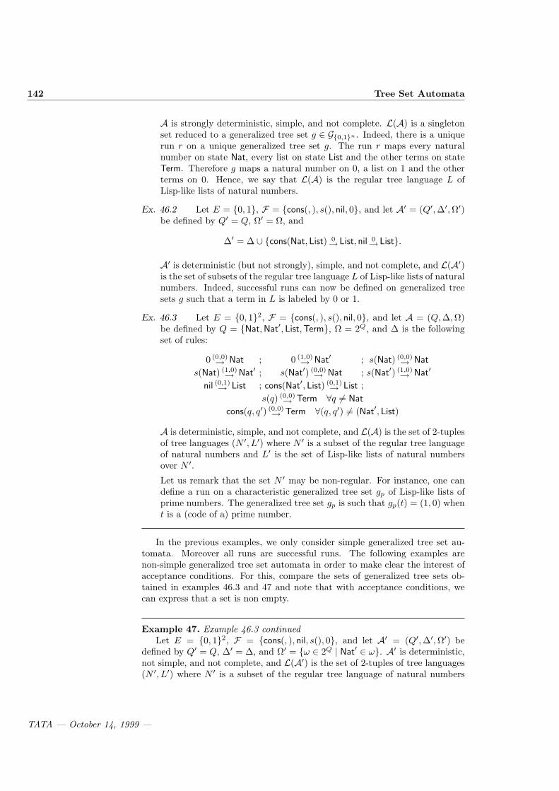
142 Tree Set Automata
A is strongly deterministic, simple, and not complete. L(A) is a singletonset reduced to a generalized tree set g ∈ G0,1n . Indeed, there is a uniquerun r on a unique generalized tree set g. The run r maps every naturalnumber on state Nat, every list on state List and the other terms on stateTerm. Therefore g maps a natural number on 0, a list on 1 and the otherterms on 0. Hence, we say that L(A) is the regular tree language L ofLisp-like lists of natural numbers.
Ex. 46.2 Let E = 0, 1, F = cons(, ), s(), nil, 0, and let A′ = (Q′, ∆′, Ω′)be defined by Q′ = Q, Ω′ = Ω, and
∆′ = ∆ ∪ cons(Nat, List) 0→ List, nil 0→ List.
A′ is deterministic (but not strongly), simple, and not complete, and L(A′)is the set of subsets of the regular tree language L of Lisp-like lists of naturalnumbers. Indeed, successful runs can now be defined on generalized treesets g such that a term in L is labeled by 0 or 1.
Ex. 46.3 Let E = 0, 12, F = cons(, ), s(), nil, 0, and let A = (Q, ∆,Ω)be defined by Q = Nat, Nat′, List,Term, Ω = 2Q, and ∆ is the followingset of rules:
0 (0,0)→ Nat ; 0 (1,0)→ Nat′ ; s(Nat) (0,0)→ Nat
s(Nat) (1,0)→ Nat′ ; s(Nat′) (0,0)→ Nat ; s(Nat′) (1,0)→ Nat′
nil (0,1)→ List ; cons(Nat′, List) (0,1)→ List ;s(q) (0,0)→ Term ∀q 6= Nat
cons(q, q′) (0,0)→ Term ∀(q, q′) 6= (Nat′, List)
A is deterministic, simple, and not complete, and L(A) is the set of 2-tuplesof tree languages (N ′, L′) where N ′ is a subset of the regular tree languageof natural numbers and L′ is the set of Lisp-like lists of natural numbersover N ′.
Let us remark that the set N ′ may be non-regular. For instance, one candefine a run on a characteristic generalized tree set gp of Lisp-like lists ofprime numbers. The generalized tree set gp is such that gp(t) = (1, 0) whent is a (code of a) prime number.
In the previous examples, we only consider simple generalized tree set au-tomata. Moreover all runs are successful runs. The following examples arenon-simple generalized tree set automata in order to make clear the interest ofacceptance conditions. For this, compare the sets of generalized tree sets ob-tained in examples 46.3 and 47 and note that with acceptance conditions, wecan express that a set is non empty.
Example 47. Example 46.3 continuedLet E = 0, 12, F = cons(, ), nil, s(), 0, and let A′ = (Q′, ∆′, Ω′) be
defined by Q′ = Q, ∆′ = ∆, and Ω′ = ω ∈ 2Q | Nat′ ∈ ω. A′ is deterministic,not simple, and not complete, and L(A′) is the set of 2-tuples of tree languages(N ′, L′) where N ′ is a subset of the regular tree language of natural numbers
TATA — October 14, 1999 —

5.2 Definitions and examples 143
and L′ is the set of Lisp-like lists of natural numbers over N ′, and N ′ 6= ∅.Indeed, for a successful r on g, there must be a term t such that r(t) = Nat′
therefore, there must be a term t labelled by (1, 0), henceforth N ′ 6= ∅.
5.2.3 Hierarchy of GTSA-recognizable languages
Let us define:
• RGTS, the class of languages recognizable by GTSA,
• RDGTS, the class of languages recognizable by deterministic GTSA,
• RSGTS, the class of languages recognizable by Simple GTSA.
The three classes defined above are proved to be different. They are alsoclosely related to classes of languages defined from the set constraint theorypoint of view.
RGTS
RDGTS
RSGTS
Figure 5.5: Classes of GTSA-recognizable languages
Classes of GTSA-recognizable languages have also different closure prop-erties. We will prove in Section 5.3.1 that RSGTS and the entire class RGTS
are closed under union, intersection, projection and cylindrification; RDGTS isclosed under complementation and intersection.
We propose three examples that illustrate the differences between the threeclasses. First, RDGTS is not a subset of RSGTS.
Example 48. Let E = 0, 1, F = f, a where a is a constant and f is unary.Let us consider the deterministic but non-simple GTSA A1 = (Q1,∆1, Ω1)where ∆1 is:
a 0→ q0, a 1→ q1,
f(q0) 0→ q0, f(q1) 0→ q0,
f(q0) 1→ q1, f(q1) 1→ q0.
and Ω1 = q0, q1, q1. Let us proove that
L(A1) = L | L 6= ∅
TATA — October 14, 1999 —

144 Tree Set Automata
is not in RSGTS.Assume that there exists a simple GTSA As with n states such that L(A1) =
L(As). Hence, As recognizes also each one of the singleton sets f i(a) for i > 0.Let us consider some i greater than n + 1, we can deduce that a run r on theGTS g associated with f i(a) maps two terms fk(a) and f l(a), k < l < i tothe same state. We have g(t) = 0 for every term t£f l(a) and r “loops” betweenfk(a) and f l(a). Therefore, one can build another run r0 on a GTS g0 suchthat g0(t) = 0 for each t ∈ T (F). Since As is simple, and since the range of r0
is a subset of the range of r, g0 is recognized, hence the empty set is recognizedwhich contradicts the hypothesis.
Basically, using simple GTSA it is not possible to enforce a state to beassumed somewhere by every run. Consequently, it is not possible to expressglobal properties of generalized tree languages such as non-emptiness.
Second, RSGTS is not a subset of RDGTS.
Example 49. Let us consider the non-deterministic but simple GTSA A2 =(Q2,∆2, Ω2) where ∆2 is:
a 0→ qf | qh, a 1→ qf | qh,
f(qf ) 1→ qf | qh, h(qh) 1→ qf | qh,
f(qh) 0→ qf | qh, h(qf ) 0→ qf | qh,
and Ω = 2qf ,qh. It is easy to prove
L(A2) = L | ∀t f(t) ∈ L ⇔ h(t) 6∈ L.
The proof that no deterministic GTSA recognizes L(A2) is left to the reader.
We terminate with an example of a non-deterministic and non-simple gen-eralized tree set automaton. This example will be used in the proof of Proposi-tion 36.
Example 50. Let A = (Q, ∆,Ω) be defined by Q = q, q′, Ω = Q, and ∆ isthe following set of rules:
a 1→ q ; a 1→ q′ ; a 0→ q′ ; f(q) 1→ q ;f(q′) 0→ q′ ; f(q′) 1→ q′ ; f(q′) 1→ q ;
The proof that A is not deterministic, not simple, and not complete, andL(A) = L ⊆ T (F) | ∃t ∈ T (F) ((t ∈ L) ∧ (∀t′ ∈ T (F) (t £ t′) ⇒ (t′ ∈ L))) isleft as an exercise to the reader.
TATA — October 14, 1999 —

5.2 Definitions and examples 145
5.2.4 Regular generalized tree sets, regular runs
As we mentioned it in Example 46.3, the set recognized by a GTSA may containGTS corresponding to non-regular languages. But regularity is of major interestfor practical reasons because it implies a GTS or a language to be finitely defined.
A generalized tree set g ∈ GE is regular if there exist a finite set R, a mapα : T (F) → R, and a map β : R → E satisfying the following two properties.
1. g = αβ (i.e. g = β α),
2. α is closed under contexts, i.e. for all context c and terms t1, t2, we have
(α(t1) = α(t2)) ⇒ (α(c[t1]) = α(c[t2]))
In the case E = 0, 1n, regular generalized tree sets will correspond ton-tuples of regular tree languages.
Although the definition of regularity leads to the definition of regular run —because a run can be considered as a generalized tree set in GQ, we use strongerconditions for a run to be regular. Indeed, regularity of generalized tree sets andregularity of runs do not correspond in general. For instance, one could defineregular runs on non-regular generalized tree sets in the case of non-stronglydeterministic generalized tree set automata, and one could define non-regularruns on regular generalized tree sets in the case of non-deterministic generalizedtree set automata.
Therefore, we only consider regular runs on regular generalized tree sets:
A run r on a generalized tree set g is regular if r ↑ g ∈ GE×Q isregular. Consequently, r and g are regular generalized tree sets.
Proposition 33. Let A be a generalized tree set automaton, if g is a regulargeneralized tree set in L(A) then there exists a regular A-run on g.
Proof. Consider a generalized tree set automaton A = (Q, ∆, Ω) over E and aregular generalized tree set g in L(A) and let r be a successful run on g. LetL be a tree language closed under the subterm relation and such that F0 ⊆ Land r(L) = r(T (F)). The generalized tree set g is regular, therefore there exista finite set R, a mapping α : T (F) → R closed under context and a mappingβ : R → E such that g = αβ. We now define a regular run r′ on g.
Let L? = L∪? where ? is a new constant symbol and let φ be the mappingfrom T (F) into Q×R×L? defined by φ(t) = (r(t), α(t), u) where u = t if t ∈ Land u = ? otherwise. Hence R′ = φ(T (F)) is a finite set because R′ ⊆ Q×R×L?.For each ρ in R′, let us fix tρ ∈ T (F) such that φ(tρ) = ρ.
The run r′ is now (regularly) defined via two mappings α′ and β′. Let β′ bethe projection from Q × R × L? into Q and let α′ : T (F) → R′ be inductivelydefined by :
∀a ∈ F0 α′(a) = φ(a);
and∀f ∈ Fp∀t1, . . . , tp ∈ T (F)
α′(f(t1, . . . , tp)) = φ(f(tα′(t1), . . . , tα′(tp))).
TATA — October 14, 1999 —

146 Tree Set Automata
Let r′ = α′β′. First we can easily prove by induction that ∀t ∈ L α′(t) = φ(t)and deduce that ∀t ∈ L r′(t) = r(t). Thus r′ and r coincide on L. It remainsto prove that (1) the mapping α′ is closed under context, (2) r′ is a run on gand (3) r′ is a successful run.
(1) From the definition of α′ we can easily derive that the mapping α′ is closedunder context.
(2) We prove that the mapping r′ = α′β′ is a run on g, that is if t = f(t1, . . . , tp)then (r′(t1), . . . , r′(tp), f, g(t), r′(t)) ∈ ∆.
Let us consider a term t = f(t1, . . . , tp). From the definitions of α′, β′, and r′,we get r′(t) = r(t′) with t′ = f(tα′(t1), . . . , tα′(tp)). The map r is a run on g,hence (r(tα′(t1)), . . . , r(tα′(tp)), f, g(t′), r(t′)) ∈ ∆, and thus it suffices to provethat g(t) = g(t′) and, for all i, r′(ti) = r(tα′(ti)).
Let i ∈ 1, . . . , p, r′(ti) = β′(α′(ti)) by definition of r′. By definition oftα′(ti), α′(ti) = φ(tα′(ti)), therefore r′(ti) = β′(φ(tα′(ti))). Now, using thedefinitions of φ and β′, we get r′(ti) = r(tα′(ti)).
In order to prove that g(t) = g(t′), we prove that α(t) = α(t′). Let π bethe projection from R′ into R. We have α(t′) = π(φ(t′)) by definition ofφ and π. We have α(t′) = π(α′(t)) using definitions of t′ and α′. Nowα(t′) = π(φ(tα′(t))) because φ(tα′(t)) = α′(t) by definition of tα′(t). And thenα(t′) = α(tα′(t)) by definition of π and φ. Therefore it remains to prove thatα(tα′(t)) = α(t). The proof is by induction on the structure of terms.
If t ∈ F0 then tα′(t) = t, so the property holds (note that this property holdsfor all t ∈ L). Let us suppose that t = f(t1, . . . , tp) and α(tα′(ti)) = α(ti) ∀i ∈1, . . . , p. First, using induction hypothesis and closure under context of α,we get
α(f(t1, . . . , tp)) = α(f(tα′(t1), . . . , tα′(tp)))
Therefore,
α(f(t1, . . . , tp)) = α(f(tα′(t1), . . . , tα′(tp)))= π(φ(f(tα′(t1), . . . , tα′(tp)))) ( def. of φ and π)= π(α′(f(t1, . . . , tp))) ( def. of α′)= π(φ(tα′(f(t1,...,tp)))) ( def. of tα′(f(t1,...,tp)))= α(tα′(f(t1,...,tp))) ( def. of φ and π).
(3) We have r′(T (F)) = r′(L) = r(L) = r(T (F)) using the definition of r′, thedefinition of L, and the equality r′(L) = r(L). The run r is a successful run.Consequently r′ is a successful run.
Proposition 34. A non-empty recognizable set of generalized tree sets containsa regular generalized tree set.
TATA — October 14, 1999 —

5.3 Closure and decision properties 147
Proof. Let us consider a generalized tree set automaton A and a successful runr on a generalized tree set g. There exists a tree language closed under thesubterm relation F such that r(F ) = r(T (F)). We define a regular run rr on aregular generalized tree set gg in the following way.
The run rr coincides with r on F : ∀t ∈ F , rr(t) = r(t) and gg(t) = g(t). Theruns rr and gg are inductively defined on T (F)\F : given q1, . . . , qp in r(T (F)),let us fix a rule f(q1, . . . , qp) l→ q such that q ∈ r(T (F)). The rule exists sincer is a run. Therefore, ∀t = f(t1, . . . , tp) 6∈ F such that rr(ti) = qi for all i ≤ p,we define rr(t) = q and gg(t) = l, following the fixed rule f(q1, . . . , qp) l→ q.
From the preceding, we can also deduce that a finite and recognizable set ofgeneralized tree sets only contains regular generalized tree sets.
5.3 Closure and decision properties
5.3.1 Closure properties
This section is dedicated to the study of classical closure properties on GTSA-recognizable languages. For all positive results — union, intersection, projec-tion, cylindrification — the proofs are constructive. We show that the class ofrecognizable sets of generalized tree sets is not closed under complementationand that non-determinism cannot be reduced for generalized tree set automata.
Set operations on sets of GTS have to be distinguished from set operationson sets of terms. In particular, in the case where E = 0, 1n, if G1 andG2 are sets of GTS in GE , G1 = (L1
1, . . . , L1n) and G2 = (L2
1, . . . , L2n), then
G1 ∪ G2 contains all GTS in G1 and G2. This is clearly different from the set(L1
1 ∪ L21, . . . , L
1n ∪ L2
n).
Proposition 35. The class RGTS is closed under intersection and union, i.e.if G1, G2 ⊆ GE are recognizable, then G1 ∪G2 and G1 ∩G2 are recognizable.
This proof is an easy modification of the classical proof of closure propertiesfor tree automata, see Chapter 1.
Proof. Let A1 = (Q1, ∆1, Ω1) and A2 = (Q2,∆2, Ω2) be two generalized treeset automata over E. Without loss of generality we suppose that Q1 ∩Q2 = ∅.
Let A = (Q, ∆, Ω) with Q = Q1 ∪Q2, ∆ = ∆1 ∪∆2, and Ω = Ω1 ∪Ω2. It isimmediate that L(A) = L(A1) ∪ L(A2).
We denote by π1 and π2 the projections from Q1 ×Q2 into respectively Q1
and Q2. Let A′ = (Q′, ∆′, Ω′) with Q′ = Q1 ×Q2, ∆′ is defined by
(f(q1, . . . , qp) l→ q ∈ ∆′) ⇔ (∀i ∈ 1, 2 f(πi(q1), . . . , πi(qp)) l→πi(q) ∈ ∆i) ,
where q1, . . . , qp, q ∈ Q′, f ∈ Fp, l ∈ E, and Ω′ is defined by
Ω′ = ω ∈ 2Q′ | πi(ω) ∈ Ωi , i ∈ 1, 2.One can easily verify that L(A′) = L(A1) ∩ L(A2) .
TATA — October 14, 1999 —

148 Tree Set Automata
Let us remark that the previous constructions also prove that the classRSGTS
is closed under union and intersection.The class languages recognizable by deterministic generalized tree set au-
tomata is closed under complementation. But, this property is false in thegeneral case of GTSA-recognizable languages.
Proposition 36. (a) Let A be a generalized tree set automaton, there existsa complete generalized tree set automaton Ac such that L(A) = L(Ac).
(b) If Acd is a deterministic and complete generalized tree set automaton, thereexists a generalized tree set automaton A′ such that L(A′) = GE−L(Acd).
(c) The class of GTSA-recognizable languages is not closed under complemen-tation.
(d) Non-determinism can not be reduced for generalized tree set automata.
Proof. (a) Let A = (Q, ∆, Ω) be a generalized tree set automaton over E and letq′ be a new state, i.e. q′ 6∈ Q. Let Ac = (Qc, ∆c, Ωc) be defined by Qc = Q∪q′,Ωc = Ω, and
∆c = ∆ ∪ (q1, . . . , qp, f, l, q′) | (q1, . . . , qp, f, l) ×Q ∩∆ = ∅;q1, . . . , qp ∈ Qc, f ∈ Fp, l ∈ E.
Ac is complete and L(A) = L(Ac). Note that Ac is simple if A is simple.
(b) Acd = (Q, ∆, Ω) be a deterministic and complete generalized tree setautomaton over E. The automaton A′ = (Q′, ∆′,Ω′) with Q′ = Q, ∆′ = ∆,and Ω′ = 2Q − Ω recognizes the set GE − L(Acd).
(c) E = 0, 1, F = c, a where a is a constant and c is of arity 1. LetG = g ∈ G0,1n | ∃t ∈ T (F) ((g(t) = 1)∧ (∀t′ ∈ T (F) (t£ t′) ⇒ (g(t′) = 1))).Clearly, G is recognizable by a non deterministic GTSA (see Example 50). LetG = G0,1n − G, we have G = g ∈ G0,1n | ∀t ∈ T (F) ∃t′ ∈ T (F) (t £ t′) ∧(g(t′) = 0) and G is not recognizable. Let us suppose that G is recognizedby an automaton A = (Q, ∆,Ω) with Card(Q) = k − 2 and let us consider thegeneralized tree set g defined by: g(ci(a)) = 0 if i = k × z for some integer z,and g(ci(a)) = 1 otherwise. The generalized tree set g is in G and we considera successful run r on g. We have r(T (F)) = ω ∈ Ω therefore there exists someinteger n such that r(g(ci(a)) | i ≤ n) = ω. Moreover we can suppose that nis a multiple of k. As Card(Q) = k − 2 there are two terms u and v in the setci(a) | n+1 ≤ i ≤ n+k−1 such that r(u) = r(v). Note that by hypothesis, forall i such that n+1 ≤ i ≤ n+k+1, g(ci(a)) = 1. Consequently, a successful rung′ could be defined from g on the generalized tree set g′ defined by g′(t) = g(t)if t = ci(a) when i ≤ n, and g′(t) = 1 otherwise. This leads to a contradictionbecause g′ 6∈ G.
(d) This result is a consequence of (b) and (c).
We will now prove the closure under projection and cylindrification. We willfirst prove a stronger lemma.
TATA — October 14, 1999 —

5.3 Closure and decision properties 149
Lemma 8. Let G ⊆ GE1 be a GTSA-recognizable language and let R ⊆ E1×E2.The set R(G) = g′ ∈ GE2 | ∃g ∈ G ∀t ∈ T (F) (g(t), g′(t)) ∈ R is recognizable.
Proof. Let A = (Q, ∆, Ω) such that L(A) = G. Let A′ = (Q′,∆′,Ω′) whereQ′ = Q, ∆′ = f(q1, . . . , qp) l′→ q | ∃l ∈ E1 f(q1, . . . , qp) l→ q ∈ ∆ and (l, l′) ∈ Rand Ω′ = Ω. We prove that R(G) = L(A′).
⊇ Let g′ ∈ L(A′) and let r′ be a successful run on g′. We construct a generalizedtree set g such that for all t ∈ T (F), (g(t), g′(t)) ∈ R and such that r′ isalso a successful A-run on g.
Let a be a constant. According to the definition of ∆′, a g′(a)→ r′(a) ∈ ∆′
implies that there exists la such that (la, g′(a)) ∈ R and a la→ r′(a) ∈ ∆.So let g(a) = la.
Let t = f(t1, . . . , tp) with ∀i r′(ti) = qi. There exists a rule f(q1, . . . , qp) g′(t)→ r′(t)in ∆′ because r′ is a run and again, from the definition of ∆′, there existslt ∈ E1 such that f(q1, . . . , qp) lt→ r′(t) in ∆ with (lt(t), g′(t)) ∈ R. So, wedefine g(t) = lt. Clearly, g is a generalized tree set and r′ is a successfulrun on g and for all t ∈ T (F), (g(t), g′(t)) ∈ R by construction.
⊆ Let g′ ∈ R(G) and let g ∈ G such that ∀t ∈ T (F) (g(t), g′(t)) ∈ R. One caneasily prove that any successful A-run on g is also a successful A′-run ong′.
Corollary 7. (a) The class of GTSA-recognizable languages is closed underprojection and cylindrification.
(b) Let G ⊆ GE and G′ ⊆ GE′ be two GTSA-recognizable languages. The setG ↑ G′ = g ↑ g′ | g ∈ G, g′ ∈ G′ is a GTSA-recognizable language inGE×E′ .
Proof. (a) The case of projection is an immediate consequence of Lemma 8using E1 = E × E′, E2 = E, and R = π where π is the projection fromE × E′ into E. The case of cylindrification is proved in a similar way.
(b) Consequence of (a) and of Proposition 35 because G ↑ G′ = π−11 (G) ∩
π−12 (G′) where π−1
1 (respectively π−12 ) is the inverse projection from E to
E × E′ (respectively from E′ to E × E′).Let us remark that the construction preserves simplicity, so RSGTS is closed
under projection and cylindrification.
We now consider the case E = 0, 1n and we give two propositions withoutproof. Proposition 37 can easily be deduced from Corollary 7. The proof ofProposition 38 would be an extension of the constructions made in Examples46.1 and 46.2.
Proposition 37. Let A and A′ be two generalized tree set automata over 0, 1n.
(a) (L1 ∪ L′1, . . . , Ln ∪ L′n) | (L1, . . . , Ln) ∈ L(A) and (L′1, . . . , L′n) ∈ L(A′)
is recognizable.
TATA — October 14, 1999 —

150 Tree Set Automata
(b) (L1 ∩ L′1, . . . , Ln ∩ L′n) | (L1, . . . , Ln) ∈ L(A) and (L′1, . . . , L′n) ∈ L(A′)
is recognizable.
(c) (L1, . . . , Ln) | (L1, . . . , Ln) ∈ L(A) is recognizable, where Li = T (F) −Li, ∀i.
Proposition 38. Let E = 0, 1n and let (F1, . . . , Fn) be a n-tuple of regulartree languages. There exist deterministic simple generalized tree set automataA , A′, and A′′ such that
• L(A) = (F1, . . . , Fn);• L(A′) = (L1, . . . , Ln) | L1 ⊆ F1, . . . , Ln ⊆ Fn;• L(A′′) = (L1, . . . , Ln) | F1 ⊆ L1, . . . , Fn ⊆ Ln.
5.3.2 Emptiness property
Theorem 41. The emptiness property is decidable in the class of generalizedtree set automata. Given a generalized tree set automaton A, it is decidablewhether L(A) = ∅.
Labels of the generalized tree sets are meaningless for the emptiness deci-sion thus we consider “label-free” generalized tree set automata. Briefly, thetransition relation of a “label-free” generalized tree set automata is a relation∆ ⊆ ∪p Qp ×Fp ×Q.
The emptiness decision algorithm for simple generalized tree set automatais straightforward. Indeed, Let ω be a subset of Q and let COND(ω) be thefollowing condition:
∀p ∀f ∈ Fp ∀q1, . . . , qp ∈ ω ∃q ∈ ω (q1, . . . , qp, f, q) ∈ ∆
We easily prove that there exists a set ω satisfying COND(ω) if and only ifthere exists an A-run. Therefore, the emptiness problem for simple generalizedtree set automata is decidable because 2Q is finite and COND(ω) is decidable.Decidability of the emptiness problem for simple generalized tree set automatais NP-complete (see Prop. 39).
The proof is more intricate in the general case, and it is not given in thisbook. Without the property of simple GTSA, we have to deal with a reachabilityproblem of a set of states since we have to check that there exists ω ∈ Ω and arun r such that r assumes exactly all the states in ω.
We conclude this section with a complexity result of the emptiness problemin the class of generalized tree set automata.
Let us consider a GTSA A with n states. The proof shows that one hasto consider at most all tree languages closed under the subterm relation of sizesmaller than B(A), a polynomial in n, in order to decide emptiness for A. Letus remark that the polynomial bound B(A) can be computed.
Proposition 39. The emptiness problem in the class of (simple) generalizedtree set automata is NP-complete.
TATA — October 14, 1999 —
5.3 Closure and decision properties 151
Proof. Let A = (Q, ∆, Ω) be a generalized tree set automaton over E. Letn = Card(Q).
We first give a non-deterministic and polynomial algorithm for decidingemptiness: (1) take a tree language F closed under the subterm relation ofsize smaller than B(A); (2) take a run r on F ; (3) compute r(F ); (4) checkwhether r(F ) = ω is a member of Ω; (5) check whether ω satisfies COND(ω).
From Theorem 41, this algorithm is correct and complete. Moreover, thisalgorithm is polynomial in n since the size of F is polynomial in n: step (2)consists in labeling the nodes of F with states following the rules of the automa-ton – so there is a polynomial number of states, step (3) consists in collectingthe states; step (4) is polynomial and non-deterministic and finally, step (5) ispolynomial.
We reduce the satisfiability problem of boolean expressions into the empti-ness problem for generalized tree set automata. We first build a generalizedtree set automaton A such that L(A) is the set of (codes of) satisfiable booleanexpressions over n variables x1, . . . , xn.
Let F = F0∪F1∪F2 where F0 = x1, . . . , xn, F1 = ¬, and F2 = ∧,∨.A boolean expression is a term of T (F). Let Bool = 0, 1 be the set of booleanvalues. Let A = (Q, ∆, Ω), be a generalized tree set automaton such thatQ = q0, q1, Ω = 2Q and ∆ is the following set of rules:
xji→ qi where j ∈ 1, . . . , n and i ∈ Bool
¬(qi) ¬i→ q¬i where i ∈ Bool
∨(qi1 , qi2) i1∨i2→ qi1∨i2 where i1, i2 ∈ Bool
∧(qi1 , qi2) i1∧i2→ qi1∧i2 where i1, i2 ∈ Bool
One can easily prove that L(A) = Lv | v is a valuation of x1, . . . , xnwhere Lv = t | t is a boolean expression which is true under v. Now, we canderive an algorithm for the satisfiability of any boolean expression e: build Ae
a strongly deterministic generalized tree set automaton such that L(A) is theset L | e ∈ L; build Ae ∩ A and decide emptiness.
We get then the reduction because Ae ∩ A is empty if and only if e is notsatisfiable.
Now, it remains to prove that the reduction is polynomial. The size of Ais 2 ∗ n + 10. The size of Ae is the length of e plus a constant. So we got theresult.
5.3.3 Other decision results
Proposition 40. The inclusion problem and the equivalence problem for deter-ministic generalized tree set automata are decidable.
Proof. These results are a consequence of the closure properties under inter-section and complementation (Propositions 35, 36), and the decidability of theemptiness property (Theorem 41).
Proposition 41. Let A be a generalized tree set automaton. It is decidablewhether or not L(A) is a singleton set.
TATA — October 14, 1999 —

152 Tree Set Automata
Proof. Let A be a generalized tree set automaton. First it is decidable whetherL(A) is empty or not (Theorem 41). Second if L(A) is non empty then a regulargeneralized tree set g in L(A) can be constructed (see the proof of Theorem41). Construct the strongly deterministic generalized tree set automaton A′such that L(A′) is a singleton set reduced to the generalized tree set g. Finally,build A∩A′ to decide the equivalence of A and A′. Note that we can build A′,since A′ is deterministic (see Proposition 36).
Proposition 42. Let L = (L1, . . . , Ln) be a tuple of regular tree language andlet A be a generalized tree set automaton over 0, 1n. It is decidable whetherL ∈ L(A).
Proof. This result just follows from closure under intersection and emptinessdecidability.
First construct a (strongly deterministic) generalized tree set automaton AL
such that L(A) is reduced to the singleton set L. Second, construct A ∩ AL
and decide whether L(A ∩AL) is empty or not.
Proposition 43. Given a generalized tree set automaton over E = 0, 1, n
and I ⊆ 1, . . . , n. The following two problems are decidable:
1. It is decidable whether or not there exists (L1, . . . , Ln) in L(A) such thatall the Li are finite for i ∈ I.
2. Let x1 . . . , xn be natural numbers. It is decidable whether or not thereexists (L1, . . . , Ln) in L(A) such that Card(Li) = xi for each i ∈ I.
The proof is technical and not given in this book. It relies on a lemma ofthe emptiness decision proof.
5.4 Applications to set constraints
In this section, we consider the satisfiability problem for systems of set con-straints. We show a decision algorithm using generalized tree set automata.
5.4.1 Definitions
Let F be a finite and non-empty set of function symbols. Let X be a set ofvariables. We consider special symbols >, ⊥, ∼, ∪, ∩ of respective arities 0, 0,1, 2, 2. A set expression is a term in TF ′(X ) where F ′ = F ∪ >,⊥,∼,∪,∩.
A set constraint is either a positive set constraint of the form e ⊆ e′ or anegative set constraint of the form e 6⊆ e′ (or ¬(e ⊆ e′)) where e and e′ are setexpressions, and a system of set constraints is defined by
∧ki=1 SCi where the
SCi are set constraints.An interpretation I is a mapping from X into 2T (F). It can immediately be
extended to set expressions in the following way:
TATA — October 14, 1999 —
5.4 Applications to set constraints 153
I(>) = T (F);I(⊥) = ∅;
I(f(e1, . . . , ep)) = f(I(e1), . . . , I(ep));I(∼ e) = T (F) \ I(e);
I(e ∪ e′) = I(e) ∪ I(e′);I(e ∩ e′) = I(e) ∩ I(e′).
We deduce an interpretation of set constraints in Bool = 0, 1, the Booleanvalues. For a system of set constraints SC, all the interpretations I such thatI(SC) = 1 are called solutions of SC. In the remainder, we will considersystems of set constraints of n variables X1, . . . , Xn. We will make no distinctionbetween a solution I of a system of set constraints and a n-tuple of tree languages(I(X1), . . . , I(Xn)). We denote by SOL(SC) the set of all solutions of a systemof set constraints SC.
5.4.2 Set constraints and automata
Proposition 44. Let SC be a system of set constraints (respectively of positiveset constraints) of n variables X1, . . . , Xn. There exists a deterministic (respec-tively deterministic and simple) generalized tree set automaton A over 0, 1n
such that L(A) is the set of characteristic generalized tree sets of the n-tuples(L1, . . . , Ln) of solutions of SC.
Proof. First we reduce the problem to a single set constraint. Let SC = C1 ∧. . . ∧ Ck be a system of set constraints. A solution of SC satisfies all theconstraints Ci. Let us suppose that, for every i, there exists a deterministicgeneralized tree set automatonAi such that SOL(Ci) = L(A). As all variables inX1, . . . , Xn do not necessarily occur in Ci, using Corollary 7, we can constructa deterministic generalized tree set automatonAn
i over 0, 1n satisfying: L(Ani )
is the set of (L1, . . . , Ln) which corresponds to solutions of Ci when restrictedto the variables of Ci. Using closure under intersection (Proposition 35), we canconstruct a deterministic generalized tree set automaton A over 0, 1n suchthat SOL(SC) = L(A).
Therefore we prove the result for a set constraint SC of n variables X1, . . . , Xn.Let E(exp) be the set of set variables and of set expression exp with a root sym-bol in F which occur in the set expression exp:
E(exp) =exp′ ∈ TF ′(X ) | exp′ £ exp and such that
either Head(exp′) ∈ F or exp′ ∈ X.
If SC ≡ exp1 ⊆ exp2 or SC ≡ exp1 6⊆ exp2 then E(SC) = E(exp1)∪E(exp2).Let us consider a set constraint SC and let ϕ be a mapping ϕ from E(SC)
into Bool. Such a mapping is easily extended first to any set expression occurringin SC and second to the set constraint SC. The symbols ∪, ∩, ∼, ⊆ and 6⊆ arerespectively interpreted as ∨, ∧, ¬, ⇒ and ¬ ⇒.
We now define the generalized tree set automaton A = (Q, ∆, Ω) over E =0, 1n.
TATA — October 14, 1999 —

154 Tree Set Automata
• The set of states is Q is the set ϕ | ϕ : E(SC) → Bool.• The transition relation is defined as follows: f(ϕ1, . . . , ϕp) l→ϕ ∈ ∆ where
ϕ1, . . . , ϕp ∈ Q, f ∈ Fp, l = (l1, . . . , ln) ∈ 0, 1n, and ϕ ∈ Q satisfies:
∀i ∈ 1, . . . , n ϕ(Xi) = li (5.6)
∀e ∈ E(SC) \ X (ϕ(e) = 1) ⇔(
e = f(e1, . . . , ep)∀i 1 ≤ i ≤ p ϕi(ei) = 1
)(5.7)
• The set of accepting sets of states Ω is defined depending on the case of apositive or a negative set constraint.
– If SC is positive, Ω = ω ∈ 2Q | ∀ϕ ∈ ω ϕ(SC) = 1;– If SC is negative, Ω = ω ∈ 2Q | ∃ϕ ∈ ω ϕ(SC) = 1.
In the case of a positive set constraint, we can choose the state set Q = ϕ |ϕ(SC) = 1 and Ω = 2Q. Consequently, A is deterministic and simple.
The correctness of this construction is easy to prove and is left to the reader.
5.4.3 Decidability results for set constraints
We now summarize results on set constraints. These results are immediateconsequences of the results of Section 5.4.2.
Proposition 45. 1. The satisfiability problem for systems of set constraintsis decidable. There exists a regular solution, that is a tuple of regular treelanguages, in any non-empty set of solutions.
2. Given two systems of set constraints SC and SC ′, it is decidable whetheror not SOL(SC) ⊆ SOL(SC ′).
3. Given a system SC of set constraints, it is decidable whether or not thereis a unique solution in SOL(SC).
4. Given a system SC of set constraints over (X1, . . . , Xn) and I ⊆ 1, . . . , n,it is decidable whether or not there is a solution (L1, . . . , Ln) ∈ SOL(SC)such that all the Li are finite for all i.
5. Given SC a system of set constraints over (X1, . . . , Xn) and a n-tuple(L1, . . . , Ln) of regular tree languages, it is decidable whether or not (L1, . . . , Ln) ∈SOL(SC).
Proof. We use Proposition 44 to encode sets of solutions of systems of set con-straints with generalized tree set automata and then, each point is deduced fromTheorem 41, or Propositions 38, 43, 40, 41.
Proposition 46. Let SC be a system of positive set constraints, it is decidablewhether or not there is a least solution in SOL(SC).
TATA — October 14, 1999 —

5.4 Applications to set constraints 155
Proof. Let SC be a system of positive set constraints. Let A be the deter-ministic, simple generalized tree set automaton over 0, 1n such that L(A) =SOL(SC) (see Proposition 44). We define a partial ordering ¹ on G0,1n by :
∀l, l′ ∈ 0, 1n l ¹ l′ ⇔ (∀i l(i) ≤ l′(i))∀g, g′ ∈ G0,1n g ¹ g′ ⇔ (∀t ∈ T (F) g(t) ¹ g′(t))
The problem we want to deal with is to decide whether or not there exists aleast generalized tree set w.r.t. ¹ in L(A). To this aim, we first build a minimalsolution if it exists, and second, we verify that this solution is unique.
Let ω be a subset of states such that COND(ω) (see the sketch of proofpage 150). Let Aω = (ω, ∆ω, 2ω) be the generalized tree set automaton Arestricted to state set ω.
Now let ∆ωmin defined by: for each (q1, . . . , qp, f) ∈ ωp × Fp, choose in
the set ∆ω one rule (q1, . . . , qp, f, l, q) such that l is minimal w.r.t. ¹. LetAω
min = (ω, ∆ωmin, 2ω). Consequently,
1. There exists only one run rω on a unique generalized tree set gω inAω
min because for all q1, . . . , qp ∈ ω and f ∈ Fp there is only one rule(q1, . . . , qp, f, l, q) in ∆ω
min;
2. the run rω on gω is regular;
3. the generalized tree set gω is minimal w.r.t. ¹ in L(Aω).
Points 1 and 2 are straightforward. The third point follows from the factthat A is deterministic. Indeed, let us suppose that there exists a run r′ on ageneralized tree set g′ such that g′ ≺ gω. Therefore, ∀t g′(t) ¹ gω(t), and thereexists (w.l.o.g.) a minimal term u = f(u1, . . . , up) w.r.t. the subterm orderingsuch that g′(u) ≺ gω(u). Since A is deterministic and ∀v ¢ u gω(v) = g′(v), wehave rω(ui) = r′(ui). Hence, the rule (rω(u1), . . . , rω(up), f, gω(u), rω(u)) is notsuch that gω(u) is minimal in ∆ω, which contradicts the hypothesis.
Consider the generalized tree sets gω for all subsets of states ω satisfyingCOND(ω). It is decidable whether or not there is a minimal generalized tree setamong them (each defines a n-tuple of regular tree languages and inclusion isdecidable for regular tree languages). Either there exists a minimal generalizedtree set g, then g is minimal in L(A) and it defines a n-tuple (F1, . . . , Fn)of regular tree languages, or not and in this case there is no least generalizedtree set g in L(A). If exists, there is a deterministic, simple generalized treeset automaton A′ such that L(A′) is the set of characteristic generalized treesets of all (L1, . . . , Ln) satisfying F1 ⊆ L1, . . . , Fn ⊆ Ln (see Proposition 38).Let A′′ be the deterministic generalized tree set automaton such that L(A′′) =L(A) ∩ L(A′) (see Proposition 35). There exists a least generalized tree setw.r.t. ¹ in L(A) if and only if the generalized tree set automata A and A′′ areequivalent. Since equivalence of generalized tree set automata is decidable (seeProposition 40) we get the result.
TATA — October 14, 1999 —

156 Tree Set Automata
5.5 Exercises
5.6 Bibliographical notes
We now survey decidability results for satisfiability of set constraints and somecomplexity issues.
Decision procedures for solving set constraints arise with [Rey69], and Mishra[Mis84]. The aim of these works was to obtain new tools for type inference andtype checking [AM91, Hei92, HJ90b, JM79, Mis84, Rey69].
First consider systems of set constraints of the form:
X1 = exp1, . . . , Xn = expn (5.8)
where the Xi are distinct variables and the expi are disjunctions of set expres-sions of the form f(Xi1 , . . . , Xip) with f ∈ Fp. These systems of set constraintsare essentially tree automata, therefore they have a unique solution and eachXi is interpreted as a regular tree language.
Suppose now that the expi are set expressions without complement symbols.Such systems are always satisfiable and have a least solution which is regular.For example, the system
Nat = s(Nat) ∪ 0X = X ∩ NatList = cons(X, List) ∪ nil
has a least solution
Nat = si(0) | i ≥ 0 , X = ∅ , List = nil.[HJ90a] investigate the class of definite set constraints which are of the form
exp ⊆ exp′, where no complement symbol occurs and exp′ contains no set opera-tion. Definite set constraints have a least solution whenever they have a solution.The algorithm presented in [HJ90a] provides a specific set of transformationrules and, when there exists a solution, the result is a regular presentation ofthe least solution, in other words a system of the form (5.8).
Solving definite set constraints is EXPTIME-complete [CP97]. Many devel-opments or improvements of Heinzte and Jaffar’s method have been proposedand some are based on tree automata [DTT97].
The class of positive set constraints is the class of systems of set constraintsof the form exp ⊆ exp′, where no projection symbol occur. In this case, when asolution exists, set constraints do not necessarily have a least solution. Severalalgorithms for solving systems in this class were proposed, [AW92] generalize themethod of [HJ90a], [GTT93] give an automata-based algorithm, and [BGW93]use the decision procedure for the first order theory of monadic predicates.Results on the computational complexity of solving systems of set constraintsare presented in a paper of [AKVW93]. The systems form a natural complexityhierarchy depending on the number of elements of F of each arity. The problemof existence of a solution of a system of positive set constraints is NEXPTIME-complete.
The class of positive and negative set constraints is the class of systems of setconstraints of the form exp ⊆ exp′ or exp 6⊆ exp′, where no projection symbol
TATA — October 14, 1999 —

5.6 Bibliographical notes 157
occur. In this case, when a solution exists, set constraints do not necessarilyhave, neither a minimal solution, nor a maximal solution. Let F = a, b().Consider the system (b(X) ⊆ X) ∧ (X 6⊆ ⊥), this system has no minimalsolution. Consider the system (X ⊆ b(X) ∪ a) ∧ (> 6⊆ X), this system hasno maximal solution. The satisfiability problem in this class turned out tobe much more difficult than the positive case. [AKW95] give a proof basedon a reachability problem involving Diophantine inequalities. NEXPTIME-completeness was proved by [Ste94]. [CP94a] gives a proof based on the ideasof [BGW93].
The class of positive set constraints with projections is the class of systems ofset constraints of the form exp ⊆ exp′ with projection symbols. Set constraintsof the form f−1
i (X) ⊆ Y can easily be solved, but the case of set constraints ofthe form X ⊆ f−1
i (Y ) is more intricate. The problem was proved decidable by[CP94b].
The expressive power of these classes of set constraints have been studied andhave been proved to be different [Sey94]. In [CK96, Koz93], an axiomatization isproposed which enlightens the reader on relationships between many approacheson set constraints.
Furthermore, set constraints have been studied in a logical and topologicalpoint of view [Koz95, MGKW96]. This last paper combine set constraints withTarskian set constraints, a more general framework for which many complexityresults are proved or recalled. Tarskian set constraints involve variables, relationand function symbols interpreted relative to a first order structure.
Topological characterizations of classes of GTSA recognizable sets, have alsobeen studied in [Tom94, Sey94]. Every set in RSGTS is a compact set and everyset in RGTS is the intersection between a compact set and an open set. Theseremarks give also characterizations for the different classes of set constraints.
TATA — October 14, 1999 —


Chapter 6
Tree transducers
6.1 Introduction
Finite state transformations of words, also called a-transducers or rational trans-ducers in the literature, model many kinds of processes, such as coffee machinesor lexical translators. But these transformations are not powerful enough tomodel syntax directed transformations, and compiler theory is an importantmotivation to the study of finite state transformations of trees. Indeed, trans-lation of natural or computing languages is directed by syntactical trees, anda translator from into HTML is a tree transducer. Unfortunately, from a the-oretical point of view, tree transducers do not inherit nice properties of wordtransducers, and the classification is very intricate. So, in the present chapterwe focus on some aspects. In Sections 6.2 and 6.3, toy examples introduce inan intuitive way different kinds of transducers. In Section 6.2, we summarizemain results in the word case. Indeed, this book is mainly concerned with trees,but the word case is useful to understand the tree case and its difficulties. Thebimorphism characterization is the ideal illustration of the link between the“machine” point of view and the “homomorphic” one. In Section 6.3, we moti-vate and illustrate bottom-up and top-down tree transducers, using compilationas leitmotiv. We precisely define and present the main classes of tree transduc-ers and their properties in Section 6.4, where we observe that general classesare not closed under composition, mainly because of alternation of copying andnondeterministic processing. Nevertheless most useful classes, as those used inSection 6.3, have closure properties. In Section 6.5 we present the homomorphicpoint of view.
Most of the proofs are tedious and are omitted. This chapter is a very incom-plete introduction to tree transducers. Tree transducers are extensively studiedfor themselves and for various applications. But as they are somewhat compli-cated objects, we focus here on the definitions and main general properties. It isusefull for every theoretical computer scientist to know main notions about treetransducers, because they are the main model of syntax directed manipulations,and that the heart of sofware manipulations and interfaces are syntax directed.Tree transducers are an essential frame to develop practical modular syntax di-rected algorithms, thought an effort of algorithmic engineering remains to do.Tree transducers theory can be fertilized by other area or can be usefull for
TATA — October 14, 1999 —

160 Tree transducers
other areas (example: Ground tree transducers for decidability of the first ordertheory of ground rewriting). We will be happy if after reading this chapter,the reader wants for further lectures, as monograph of Z. Fulop and H. Vogler(december 1998 [FV98]).
6.2 The word case
6.2.1 Introduction to rational transducers
We suppose that the reader roughly knows popular notions of language theory:homomorphisms on words, finite automata, rational expressions, regular gram-mars. See for example the recent survey of A. Mateescu and A. Salomaa [MS96].A rational transducer is a finite word automaton W with output. In a wordautomaton, a transition rule f(q) → q′(f) means “if W is in some state q, if itreads the input symbol f , then it enters state q′ and moves its head one symbolto the right”. For defining a rational transducer, it suffices to add an output,and a transition rule f(q) → q′(m) means “if the transducer is in some stateq, if it reads the input symbol f , then it enters state q′, writes the word m onthe output tape, and moves its head one symbol to the right”. Remark thatwith these notations, we identify a finite automaton with a rational transducerwhich writes what it reads. Note that m is not necessarily a symbol but canbe a word, including the empty word. Furthermore, we assume that it is notnecessary to read an input symbol, i.e. we accept transition rules of the formε(q) → q′(m) (ε denotes the empty word).
Graph presentations of finite automata are popular and convenient. So it isfor rational transducers. The rule f(q) → q′(m) will be drawn
f/mq q′
Example 51. (Language L1) Let F = 〈, 〉, ; , 0, 1, A, ..., Z. In the following,we will consider the language L1 defined on F by the regular grammar (theaxiom is program):program → 〈 instructinstruct → LOAD register | STORE register | MULT register
→ | ADD registerregister → 1tailregistertailregister → 0tailregister | 1tailregister | ; instruct | 〉
( a → b|c is an abbreviation for the set of rules a → b, a → c)L1 is recognized by deterministic automaton A1 of Figure 6.1. Semantic of
L1 is well known: LOAD i loads the content of register i in the accumulator;STORE i stores the content of the accumulator in register i; ADD i adds in theaccumulator the content of the accumulator and the content of register i; MULTi multiplies in the accumulator the content of the accumulator and the contentof register i.
TATA — October 14, 1999 —

6.2 The word case 161
D
TS
〈
end
Begin
Instruct
O AL
Tailregister
Register
A
M
O R E
TLU
D D1
0,1
〉;
Figure 6.1: A recognizer of L1
TATA — October 14, 1999 —

162 Tree transducers
A rational transducer is a tuple R = (Q,F ,F ′, Qi, Qf ,∆) where Q is a setof states, F and F ′ are finite nonempty sets of input letters and output letters,Qi, Qf ⊆ Q are sets of initial and final states and ∆ is a set of transductionrules of the following type:
f(q) → q′(m),
where f ∈ F ∪ ε , m ∈ F ′∗ , q, q′ ∈ Q.R is ε-free if there is no rule f(q) → q′(m) with f = ε in ∆.The move relation →R is defined by: let t, t′ ∈ F∗, u ∈ F ′∗ , q, q′ ∈ Q,
f ∈ F , m ∈ F ′∗ ,
(tqft′, u)→R
(tfq′t, um) ⇔ f(q) → q′(m) ∈ ∆,
and →∗R is the reflexive and transitive closure of →R. A (partial) transduction
of R on tt′t′′ is a sequence of move steps of the form (tqt′t′′, u)→∗R(tt′q′t′′, uu′).
A transduction of R from t ∈ F∗ into u ∈ F ′∗ is a transduction of the form(qt, ε)→∗
R(tq′, u) with q ∈ Qi and q′ ∈ Qf .The relation TR induced by R can now be formally defined by:
TR = (t, u) | (qt, ε) ∗→R
(tq′, u) with t ∈ F∗, u ∈ F ′∗ , q ∈ Qi, q′ ∈ Qf.
A relation in F∗ ×F ′∗ is a rational transduction if and only if it is inducedby some rational transducer. We also need the following definitions: let t ∈ F∗,TR(t) = u | (t, u) ∈ TR. The translated of a language L is obviously thelanguage defined by TR(L) = u | ∃t ∈ L, u ∈ TR(t).
Example 52.Ex. 52.1 Let us name French-L1 the translation of L1 in French (LOAD is
translated into CHARGER and STORE into STOCKER). Transducer of Figure 6.2realizes this translation. This example illustrates the use of rational trans-ducers as lexical transducers.
Ex. 52.2 Let us consider the rational transducer Diff defined by Q = qi, qs, ql, qd,F = F ′ = a, b, Qi = qi, Qf = qs, ql, qd, and ∆ is the set of rules:
type i a(qi) → qi(a), b(qi) → qi(b)
type s ε(qi) → qs(a), ε(qi) → qs(b), ε(qs) → qs(a), ε(qs) → qs(b)
type l a(qi) → ql(ε), b(qi) → ql(ε), a(ql) → ql(ε), b(ql) → ql(ε)
type d a(qi) → qd(b), b(qi) → qd(a), a(qd) → qd(ε), b(qd) → qd(ε),ε(qd) → qd(a), ε(qd) → qd(b).
It is easy to prove that TDiff = (m,m′) | m 6= m′,m, m′ ∈ a, b∗.
We give without proofs some properties of rational transducers. For moredetails, see [Sal73] or [MS96] and Exercises 66, 67, 69 for 1, 4 and 5. Thehomomorphic approach presented in the next section can be used as an elegantway to prove 2 and 3 (Exercise 71).
Proposition 47 (Main properties of rational transducers).
TATA — October 14, 1999 —

6.2 The word case 163
〉/〉
end
Begin
Instruct
O/ε
Tailregister
Register
A/ε
R/ε
L/ε
D/ε0/0
;/;
1/1
D/CHARGERA/ε
S/ε T/ε 0/ε
1/1
D/ε
T/MULTM/ε U/ε
L/ε
〈/〈E/STOCKER
Figure 6.2: A rational transducer from L1 into French-L1.
TATA — October 14, 1999 —

164 Tree transducers
1. The class of rational transductions is closed under union but not closedunder intersection.
2. The class of rational transductions is closed under composition.
3. Regular languages and context-free languages are closed under rationaltransduction.
4. Equivalence of rational transductions is undecidable.
5. Equivalence of deterministic rational transductions is decidable.
6.2.2 The homomorphic approach
A bimorphism is defined as a triple B = (Φ, L, Ψ) where L is a recognizablelanguage and Φ and Ψ are homomorphisms. The relation induced by B (alsodenoted by B) is defined by B = (Φ(t), Ψ(t)) | t ∈ L. Bimorphism (Φ, L, Ψ)is ε-free if Φ is ε-free (an homomorphism is ε-free if the image of a letter isnever reduced to ε). Two bimorphisms are equivalent if they induce the samerelation.
We can state the following theorem, generally known as Nivat Theorem [Niv68](see Exercises 70 and 71 for a sketch of proof).
Theorem 42 (Bimorphism theorem). Given a rational transducer, an equiv-alent bimorphism can be constructed. Conversely, any bimorphism defines arational transduction. Construction preserve ε-freeness.
Example 53.Ex. 53.1 The relation (a(ba)n, an) | n ∈ N ∪ ((ab)n, b3n) | n ∈ N is
processed by transducer R and bimorphism B of Figure 6.3
b/ε
a/a
a/ε
a/ε
a/ε
b/bbbb/bbb
Φ(A) = a
Φ(B) = ba
Φ(C) = ab
Ψ(A) = ε
Ψ(B) = a
Ψ(C) = bbb
C
B
C
A
ΨΦ
Figure 6.3: Transducer R and an equivalent bimorphism B = (Φ(t),Ψ(t)) | t ∈AB∗ + CC∗.
Ex. 53.2 Automaton L of Figure 6.4 and morphisms Φ and Ψ bellow definea bimorphism equivalent to transducer of Figure 6.2
TATA — October 14, 1999 —

6.3 Introduction to tree transducers 165
Φ(β) = 〈 Φ(λ) = LOAD Φ(σ) = STORE Φ(µ) = MULTΦ(α) = ADD Φ(ρ) =; Φ(ω) = 1 Φ(ζ) = 0Φ(θ) =〉Ψ(β) = 〈 Ψ(λ) = CHARGER Ψ(σ) = STOCKER Ψ(µ) = MULTΨ(α) = ADD Ψ(ρ) =; Ψ(ω) = 1 Ψ(ζ) = 0Ψ(θ) =〉
θend
Register
Instruct
Tailregister
Begin λ, σ, µ, α
β
ρ
ω
ζ, ω
Figure 6.4: The control automaton L.
Nivat characterization of rational transducers makes intuitive sense. Au-tomaton L can be seen as a control of the actions, morphism Ψ can be seen asoutput function and Φ−1 as an input function. Φ−1 analyses the input — it isa kind of part of lexical analyzer — and it generates symbolic names; regulargrammatical structure on theses symbolic names is controlled by L. Exam-ples 53.1 and 53.2 are an obvious illustration. L is the common structure toEnglish and French versions, Φ generates the English version and Ψ generatesthe French one. This idea is the major idea of compilation, but compilation ofcomputing languages or translation of natural languages are directed by syntax,that is to say by syntactical trees. This is the motivation of the rest of the chap-ter. But unfortunately, from a formal point of view, we will lose most of thebest results of the word case. Power of non-linear tree transducers will explainin part this complication, but even in the linear case, there is a new phenom-ena in trees, the understanding of which can be introduced by the “problem ofhomomorphism inversion” that we describe in Exercise 72.
6.3 Introduction to tree transducers
Tree transducers and their generalizations model many syntax directed trans-formations (see exercises). We use here a toy example of compiler to illustratehow usual tree transducers can be considered as modules of compilers.
We consider a simple class of arithmetic expressions (with usual syntax) assource language. We suppose that this language is analyzed by a LL1 parser. Weconsider two target languages: L1 defined in Example 51 and an other languageL2. A transducer A translates syntactical trees in abstract trees (Figure 6.5).A second tree transducer R illustrates how tree transducers can be seen as
TATA — October 14, 1999 —

166 Tree transducers
part of compilers which compute attributes over abstract trees. It decoratesabstract trees with numbers of registers (Figure 6.7). Thus R translates abstracttrees into attributed abstract trees. After that, tree transducers T1 and T2
generate target programs in L1 and L2, respectively, starting from attributedabstract trees (Figures 6.7 and 6.8). This is an example of nonlinear transducer.Target programs are yields of generated trees. So composition of transducersmodel succession of compilation passes, and when a class of transducers is closedby composition (see section 6.4), we get universal constructions to reduce thenumber of compiler passes and to meta-optimize compilers.
We now define the source language. Let us consider the terminal alphabet(, ),+,×, a, b, . . . , z. First, the context-free word grammar G1 is defined byrules (E is the axiom):
E → M | M + EM → F | F ×MF → I | (E)I → a | b | · · · | z
Another context-free word grammar G2 is defined by (E is the axiom):
E → ME′
E′ → +E | εM → FM ′
M ′ → ×M | εF → I | (E)I → a | b | · · · | z
Let E be the axiom of G1 and G2. The semantic of these two grammarsis obvious. It is easy to prove that they are equivalent, i.e. they define thesame source language. On the one hand, G1 is more natural, on the otherhand G2 could be preferred for syntactical analysis reason, because G2 is LL1and G1 is not LL. We consider syntactical trees as derivation trees for thetree grammar G2. Let us consider word u = (a + b) × c. u of the sourcelanguage. We define the abstract tree associated with u as the tree ×(+(a, b), c)defined over F = +(, ),×(, ), a, b, c. Abstract trees are ground terms overF . Evaluate expressions or compute attributes over abstract trees than oversyntactical trees. The following transformation associates with a syntacticaltree t its corresponding abstract tree A(t).
I(x) → x F (x) → xM(x,M ′(ε)) → x E(x,E′(ε)) → x
M(x,M ′(×, y)) → ×(x, y) E(x,E′(+, y)) → +(x, y)F ((, x, )) → x
We have not precisely defined the use of the arrow →, but it is intuitive.Likewise we introduce examples before definitions of different kinds of tree trans-ducers (section 6.4 supplies a formal frame).
To illustrate nondeterminism, let us introduce two new transducers A and A′.Some brackets are optional in the source language, hence A′ is nondeterministic.Note that A works from frontier to root and A′ works fromm root to frontier.
TATA — October 14, 1999 —

6.3 Introduction to tree transducers 167
A : an example of bottom-up tree transducer
The following linear deterministic bottom-up tree transducer A carries outtransformation of derivation trees for G2 into the corresponding abstract trees.Empty word ε is identified as a constant symbol in syntactical trees. States ofA are q, qε, qI , qF , qM ′ε, qE′ε, qE , q×, qM ′×, q+, qE′+, q(, and q). Final state isqE . The set of transduction rules is:
a → q(a) b → q(b)c → q(c) ε → qε(ε)) → q)()) ( → q((()
+ → q+(+) × → q×(×)I(q(x)) → qI(x) F (qI(x)) → qF (x)
M ′(qε(x)) → qM ′ε(x) E′(qε(x)) → qE′ε(x)M(qF (x), qM ′ε(y)) → qM (x) E(qM (x), qE′ε(y)) → qE(x)M ′(q×(x), qM (y)) → qM ′×(y) M(qF (x), qM ′×(y)) → qM (×(x, y))E′(q+(x), qE(y)) → qE′+(y) E(qM (x), qE′+(y)) → qE(+(x, y))
F (q((x), qE(y), q)(z)) → qF (y)
The notion of (successful) run is an intuitive generalization of the notionof run for finite tree automata. The reader should note that FTAs can beconsidered as a special case of bottom-up tree transducers whose output is equalto the input. We give in Figure 6.5 an example of run of A which translatesderivation tree t which yields (a + b)× c for context-free grammar G2 into thecorresponding abstract tree ×(+(a, b), c).
t→∗A
(
q(
a
qM
b
qE′+
E
)
q)
F
ε
qM ′×
M
c
qE′ε
E
→∗A
a b
+
qF
ε
qM ′×
M
c
qE′ε
E
→∗A
a b
+ c
×
qE
Figure 6.5: Example of run of A
A′ : an example of top-down tree transducer
The inverse transformation A−1, which computes the set of derivation trees ofG2 associated with an abstract tree, is computed by a nondeterministic top-down tree transducer A′. The states of A′ are qE , qF , qM . The initial state isqE . The set of transduction rules is:
TATA — October 14, 1999 —

168 Tree transducers
qE(x) → E(qM (x), E′(ε)) qE(+(x, y)) → E(qM (x), E′(+, qE(y)))qM (x) → M(qF (x),M ′(ε)) qM (×(x, y)) → M(qF (x),M ′(×, qM (y)))qF (x) → F ((, qE(x), )) qF (a) → F (I(a))qF (b) → F (I(b)) qF (c) → F (I(c))
Transducer A′ is nondeterministic because there are ε-rules like qE(x) →E(qM (x), E′(ε)). We give in Figure 6.6 an example of run of A′ which transformsabstract tree +(a,×(b, c)) into a syntactical tree t′ of the word a + b× c.
a
b c
×
+
qE
→A′
a
qM
+
b c
×
qE
E′
E
→∗A′
a
I
F
ε
M ′
M
+
b c
×
qE
E′
E
→∗A′ t
′
Figure 6.6: Example of run of A′
Compilation
The compiler now transforms abstract trees into programs for some target lan-guages. We consider two target languages. The first one is L1 of Example 51.To simplify, we omit “;”, because they are not necessary — we introduced semi-colons in Section 6.2 to avoid ε-rules, but this is a technical detail, because word(and tree) automata with ε-rules are equivalent to usual ones. The second targetlanguage is an other very simple language L2, namely sequences of two instruc-tions +(i, j, k) (put the sum of contents of registers i and j in the register k) and×(i, j, k). In a first pass, we attribute to each node of the abstract tree the min-imal number of registers necessary to compute the corresponding subexpressionin the target language. The second pass generates target programs.
First pass: computation of register numbers by a deterministic linear bottom-up transducer R.
States of a tree automaton can be considered as values of (finitely val-ued) attributes, but formalism of tree automata does not allow decoratingnodes of trees with the corresponding values. On the other hand, this dec-oration is easy with a transducer. Computation of finitely valued inherited(respectively synthesized) attributes is modeled by top-down (respectivelybottom-up) tree transducers. Here, we use a bottom-up tree transducerR. States of R are q0, . . . , qn. All states are final states. The set of rules
TATA — October 14, 1999 —

6.4 Properties of tree transducers 169
is:
a → q0(a) b → q0(b)c → q0(c)
+(qi(x), qi(y)) → qi+1( +i+1(x, y)) ×(qi(x), qi(y)) → qi+1( +
i 1× (x, y))if i > j+(qi(x), qj(y)) → qi( +
i (x, y) ×(qi(x), qj(y)) → qi(×i (x, y))if i < j, we permute the order of subtrees+(qi(x), qj(y)) → qj( +
j (y, x)) ×(qi(x), qj(y)) → qj(×j (y, x))
A run t→∗R qi(u) means that i registers are necessary to evaluate t. Root
of t is then relabelled in u by symbol +i or ×
i .
Second pass: generation of target programs in L1 or L2, by top-down de-terministic transducers T1 and T2. T1 contains only one state q. Setof rules of T1 is:
q( +i (x, y)) → ¦(q(x), STOREi, q(y), ADDi, STOREi)
q(×i (x, y)) → ¦(q(x), STOREi, q(y), MULTi, STOREi)q(a) → ¦(LOAD, a)q(b) → ¦(LOAD, b)q(c) → ¦(LOAD, c)
where ¦(, , , , ) and ¦(, ) are new symbols.
State set of T2 is q, q′ where q′ is the initial state. Set of rules of T2 is:
q( +i (x, y)) → #(q(x), q(y),+, (, q′(x), q′(y), i, )) q′( +
i (x, y)) → iq(×i (x, y)) → #(q(x), q(y),×, (, q′(x), q′(y), i, )) q′(×i (x, y)) → i
q(a) → ε q′(a) → aq(b) → ε q′(b) → bq(c) → ε q′(c) → c
where # is a new symbol of arity 8.
The reader should note that target programs are words formed with leavesof trees, i.e. yields of trees. Examples of transductions computed by T1
and T2 are given in Figures 6.7 and 6.8. The reader should also note thatT1 is an homomorphism. Indeed, an homomorphism can be considered asa particular case of deterministic transducer, namely a transducer withonly one state (we can consider it as bottom-up as well as top-down). Thereader should also note that T2 is deterministic but not linear.
6.4 Properties of tree transducers
6.4.1 Bottom-up tree transducers
We now give formal definitions. In this section, we consider academic examples,without intuitive semantic, to illustrate phenomena and properties. Tree trans-ducers are both generalization of word transducers and tree automata. We first
TATA — October 14, 1999 —
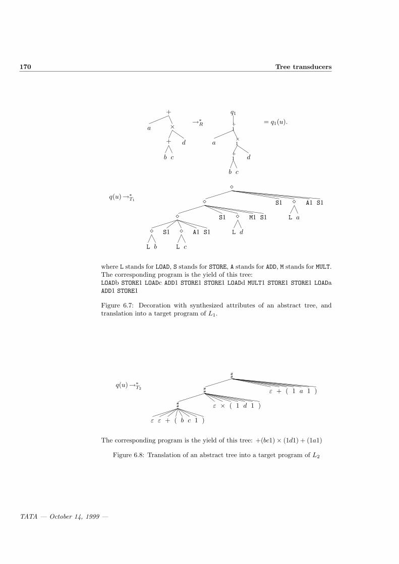
170 Tree transducers
a
b c
+ d
×
+→∗
R
a
b c
+1 d
×1
+1
q1
= q1(u).
q(u)→∗T1
L b
¦ S1
L c
¦ A1 S1
¦ S1
L d
¦ M1 S1
¦ S1
L a
¦ A1 S1
¦
where L stands for LOAD, S stands for STORE, A stands for ADD, M stands for MULT.The corresponding program is the yield of this tree:LOADb STORE1 LOADc ADD1 STORE1 STORE1 LOADd MULT1 STORE1 STORE1 LOADaADD1 STORE1
Figure 6.7: Decoration with synthesized attributes of an abstract tree, andtranslation into a target program of L1.
q(u)→∗T2
ε ε + ( b c 1 )
] ε × ( 1 d 1 )
] ε + ( 1 a 1 )
]
The corresponding program is the yield of this tree: +(bc1)× (1d1) + (1a1)
Figure 6.8: Translation of an abstract tree into a target program of L2
TATA — October 14, 1999 —

6.4 Properties of tree transducers 171
consider bottom-up tree transducers. A transition rule of a NFTA is of the typef(q1(x1), . . . , qn(xn)) → q(f(x1, . . . , xn)). Here we extend the definition (as wedid in the word case), accepting to change symbol f into any term.
A bottom-up Tree Transducer (NUTT) is a tuple U = (Q,F ,F ′, Qf , ∆)where Q is a set of (unary) states, F and F ′ are finite nonempty sets of inputsymbols and output symbols, Qf ⊆ Q is a set of final states and ∆ is a set oftransduction rules of the following two types:
f(q1(x1), . . . , qn(xn)) → q(u) ,
where f ∈ Fn, u ∈ T (F ′,Xn), q, q1, . . . , qn ∈ Q , or
q(x1) → q′(u) (ε-rule),
where u ∈ T (F ′,X1), q, q′ ∈ Q.As for NFTA, there is no initial state, because when a symbol is a leave a
(i.e. a constant symbol), transduction rules are of the form a → q(u), whereu is a ground term. These rules can be considered as “initial rules”. Lett, t′ ∈ T (F ∪ F ′ ∪Q). The move relation →U is defined by:
t→U
t′ ⇔
∃f(q1(x1), . . . , qn(xn)) → q(u) ∈ ∆∃C ∈ C(F ∪ F ′ ∪Q)∃u1, . . . , un ∈ T (F ′)t = C[f(q1(u1), . . . , qn(un))]t′ = C[q(ux1←u1, . . . , xn←un)]
This definition includes the case of ε-rule as a particular case. The reflexiveand transitive closure of →U is →∗
U . A transduction of U from a ground termt ∈ T (F) to a ground term t′ ∈ T (F ′) is a sequence of move steps of the formt→∗
U q(t′), such that q is a final state. The relation induced by U is the relation(also denoted by U) defined by:
U = (t, t′) | t ∗→U
q(t′), t ∈ T (F), t′ ∈ T (F ′), q ∈ Qf.
The domain of U is the set t ∈ T (F) | (t, t′) ∈ U. The image by U of aset of ground terms L is the set U(L) = t′ ∈ T (F ′) | ∃t ∈ L, (t, t′) ∈ U.
A transducer is ε-free if it contains no ε-rule. It is linear if all tran-sition rules are linear (no variable occurs twice in the right-hand side). Itis non-erasing if, for every rule, at least one symbol of F ′ occurs in theright-hand side. It is said to be complete (or non-deleting) if, for every rulef(q1(x1), . . . , qn(xn)) → q(u) , for every xi(1 ≤ i ≤ n), xi occurs at least oncein u. It is deterministic (DUTT) if it is ε-free and there is no two rules withthe same left-hand side.
Example 54.Ex. 54.1 Tree transducer A defined in Section 6.3 is a linear DUTT. Tree
transducer R in Section 6.3 is a linear and complete DUTT.
Ex. 54.2 States of U1 are q, q′; F = f(), a; F ′ = g(, ), f(), f ′(), a; q′ isthe final state; the set of transduction rules is:
a → q(a)f(q(x)) → q(f(x)) | q(f ′(x)) | q′(g(x, x))
TATA — October 14, 1999 —

172 Tree transducers
U1 is a complete, non linear NUTT. We now give the transductions ofthe ground term f(f(f(a))). For the sake of simplicity, fffa stands forf(f(f(a))). We have:
U1(fffa) = g(ffa, ffa), g(ff ′a, ff ′a), g(f ′fa, f ′fa), g(f ′f ′a, f ′f ′a).
U1 illustrates an ability of NUTT, that we describe following Gecseg andSteinby.
B1- “Nprocess and copy” A NUTT can first process an input sub-tree nondeterministically and then make copies of the resultingoutput tree.
Ex. 54.3 States of U2 are q, q′; F = F ′ = f(), f ′(), a; q is the final state;the set of transduction rules is defined by:
a → q(a)f(q(x)) → q′(a)
f ′(q′(x)) → q(a)
U2 is a non complete DUTT. The tree transformation induced by U2 is
(t, a) | t is accepted by the DFTA of final state q and rulesa → q(a), f(q(x)) → q′(f(x)), f ′(q′(x)) → q(f ′(x))
.
B2- “check and delete” A NUTT can first check regular con-straints on input subterms and delete these subterms afterwards.
Bottom-up tree transducers translate the input trees from leaves to root, sobottom-up tree transducers are also called frontier-to-root transducers. Top-down tree transducers work in opposite direction.
6.4.2 Top-down tree transducers
A top-down Tree Transducer (NDTT) is a tuple D = (Q,F ,F ′, Qi, ∆) whereQ is a set of (unary) states, F and F ′ are finite nonempty sets of input sym-bols and output symbols, Qi ⊆ Q is a set of initial states and ∆ is a set oftransduction rules of the following two types:
q(f(x1, . . . , xn)) → u[q1(xi1), . . . , qp(xip)] ,
where f ∈ Fn, u ∈ Cp(F ′), q, q1, . . . , qp ∈ Q, , xi1 , . . . , xip ∈ Xn, or
q(x) → u[q1(x), . . . , qp(x)] (ε-rule),
where u ∈ Cp(F ′), q, q1, . . . , qp ∈ Q, x ∈ X .As for top-down NFTA, there is no final state, because when a symbol is a
leave a (i.e. a constant symbol), transduction rules are of the form q(a) → u,where u is a ground term. These rules can be considered as “final rules”. Lett, t′ ∈ T (F ∪ F ′ ∪Q). The move relation →D is defined by:
TATA — October 14, 1999 —

6.4 Properties of tree transducers 173
t→D
t′ ⇔
∃q(f(x1, . . . , xn)) → u[q1(xi1), . . . , qp(xip)] ∈ ∆
∃C ∈ C(F ∪ F ′ ∪Q)∃u1, . . . , un ∈ T (F)t = C[q(f(u1, . . . , un))]t′ = C[u[q1(v1), . . . , qp(vp)])] where vj = uk if xij = xk
This definition includes the case of ε-rule as a particular case. →∗D is the
reflexive and transitive closure of →D. A transduction of D from a ground termt ∈ T (F) to a ground term t′ ∈ T (F ′) is a sequence of move steps of the formq(t)→∗
D t′, where q is an initial state. The transformation induced by D is therelation (also denoted by D) defined by:
D = (t, t′) | q(t) ∗→D
t′, t ∈ T (F), t′ ∈ T (F ′), q ∈ Qi.
The domain of D is the set t ∈ T (F) | (t, t′) ∈ D. The image of a setof ground terms L by D is the set D(L) = t′ ∈ T (F ′) | ∃t ∈ L, (t, t′) ∈ D.ε-free, linear, non-erasing, complete (or non-deleting), deterministic top-downtree transducers are defined as in the bottom-up case.
Example 55.Ex. 55.1 Tree transducers A′, T1, T2 defined in Section 6.3 are examples of
NDTT.
Ex. 55.2 Let us now define a non-deterministic and non linear NDTT D1.States of D1 are q, q′. The set of input symbols is F = f(), a. The set ofoutput symbols is F ′ = g(, ), f(), f ′(), a. The initial state is q. The setof transduction rules is:
q(f(x)) → g(q′(x), q′(x)) (copying rule)q′(f(x)) → f(q′(x)) | f ′(q′(x)) (non deterministic relabeling)
q′(a) → a
D1 transduces f(f(f(a))) (or briefly fffa) into the set of 16 trees:
g(ffa, ffa), g(ffa, ff ′a), g(ffa, f ′fa), . . . , g(f ′f ′a, f ′fa), g(f ′f ′a, f ′f ′a).
D1 illustrates a new property.
D- “copy and Nprocess” A NDTT can first make copies of aninput subtree and then process different copies independently andnondeterministically .
TATA — October 14, 1999 —

174 Tree transducers
6.4.3 Structural properties
In this section, we use tree transducers U1, U2 and D1 of the previous section inorder to point out differences between top-down and bottom-up tree transducers.
Theorem 43 (Comparison Theorem).
1. There is no top-down tree transducer equivalent to U1 or to U2.
2. There is no bottom-up tree transducer equivalent to D1.
3. Any linear top-down tree transducer is equivalent to a linear bottom-up treetransducer. In the linear complete case, classes of bottom-up and top-downtree transducers are equal.
It is not hard to verify that neither NUTT nor NDTT are closed undercomposition. Therefore, comparison of D-property “copy and Nprocess” andU -property “Nprocess and copy” suggests an important question:
does alternation of copying and non-determinism induces an infinitehierarchy of transformations?
The answer is affirmative [Eng78, Eng82], but it was a relatively long-standingopen problem. The fact that top-down transducers copy before non-deterministicprocesses, and bottom-up transducers copy after non-deterministic processes(see Exercise 76) suggests too that we get by composition two intricate infinitehierarchies of transformation. The following theorem summarizes results.
Theorem 44 (Hierarchy theorem). By composition of NUTT, we get an in-finite hierarchy of transformations. Any composition of n NUTT can be pro-cessed by composition of n+1 NDTT, and conversely (i.e. any composition of nNDTT can be processed by composition of n + 1 NUTT).
Transducer A′ of Section 6.3 shows that it can be useful to consider ε-rules,but usual definitions of tree transducers in literature exclude this case of nondeterminism. This does not matter, because it is easy to check that all importantresults of closure or non-closure hold simultaneously for general classes and ε-free classes. Deleting is also a minor phenomenon. Indeed, it gives rise to the“check and delete” property, which is specific to bottom-up transducers, butit does not matter for hierarchy theorem, which remains true if we considercomplete transducers.
Section 6.3 suggests that for practical use, non-determinism and non-linearityare rare. Therefore, it is important to note than if we suppose linearity or deter-minism, hierarchy of Theorem 45 collapses. Following results supply algorithmsto compose or simplify transducers.
Theorem 45 (Composition Theorem).
1. The class of linear bottom-up transductions is closed under composition.
2. The class of deterministic bottom-up transductions is closed under com-position.
3. The class of linear top-down transductions is included in the class of lin-ear bottom-up transductions. These classes are equivalent in the completecase.
TATA — October 14, 1999 —
6.5 Homomorphisms and tree transducers 175
4. Any composition of deterministic top-down transductions is equivalent toa deterministic complete top-down transduction composed with a linearhomomorphism.
The reader should note that bottom-up determinism and top-down deter-minism are incomparable (see Exercise 73).
Recognizable tree languages play a crucial role because derivation trees ofcontext-free word grammars are recognizable. Fortunately, we get:
Theorem 46 (Recognizability Theorem). The domain of a tree transduceris a recognizable tree language. The image of a recognizable tree language by alinear tree transducer is recognizable.
6.4.4 Complexity properties
We present now some decidability and complexity results. As for structuralproperties, the situation is more complicated than in the word case, especiallyfor top-down tree transducers. Most of problems are untractable in the worstcase, but empirically “not so much complex” in real cases, though there is a lakeof “algorithmic engineering” to get performant algorithms. As in the word case,emptiness is decidable, and equivalence in undecidable in the general case but isdecidable in the k-valued case (a transducer is k-valued if there is no tree whichis transduced in more than k different terms; so a deterministic transducer is aparticular case of 1-valued transducer).
Theorem 47 (Recidability and complexity). Emptiness of tree transduc-tions is decidable. Equivalence of k-valued tree transducers is decidable.
Emptiness for bottom-up transducers is essentially the same as emptinessfor tree automata and therefore PTIME complete. Emptiness for top-downautomata, however, is essentially the same as emptiness for alternating topdowntree automata, giving DEXPTIME completeness for emptiness. The complexityPTIME for testing single-valuedness in the bottom-up case is contained in Seidl[Sei92]. Ramsey theory gives combinatorial properties onto which equivalencetests for k-valued tree transducers [Sei94a].
Theorem 48 (Equivalence Theorem). Equivalence of deterministic tree trans-ducers is decidable.
6.5 Homomorphisms and tree transducers
Exercise 75 illustrates how decomposition of transducers using homomorphismscan help to get composition results, but we are far from the nice bimorphismtheorem of the word case, and in the tree case, there is no illuminating the-orem, but many complicated partial statements. Seminal paper of Engelfriet[Eng75] contains a lot of decomposition and composition theorems. Here, weonly present the most significant results.
A delabeling is a linear, complete, and symbol-to-symbol tree homomor-phism (see Section 1.4). This very special kind of homomorphism changes onlythe label of the input letter and possibly order of subtrees. Definition of tree
TATA — October 14, 1999 —

176 Tree transducers
bimorphisms is not necessary, it is the same as in the word case. We get the fol-lowing characterization theorem. We say that a bimorphism is linear, (respec-tively complete, etc) if the two morphisms are linear, (respectively complete,etc).
Theorem 49. The class of bottom-up tree transductions is equivalent to theclass of bimorphisms (Φ, L,Ψ) where Φ is a delabeling.
Relation defined by (Φ, L, Ψ) is computed by a transduction which is linear(respectively complete, ε-free) if Ψ is linear (respectively complete, ε-free).
Remark that Nivat Theorem illuminates the symmetry of word transduc-tions: the inverse relation of a rational transduction is a rational transduction.In the tree case, non-linearity obviously breaks this symmetry, because a treetransducer can copy an input tree and process several copies, but it can nevercheck equality of subtrees of an input tree. If we want to consider symmetricrelations, we have two main situations. In the non-linear case, it is easy to provethat composition of two bimorphisms simulates a Turing machine. In the linearand the linear complete cases, we get the following results.
Theorem 50 (Tree Bimorphisms). .
1. The class LCFB of linear complete ε-free tree bimorphisms satisfies LCFB ⊂LCFB2 = LCFB3.
2. The class LB of linear tree bimorphisms satisfies LB ⊂ LB2 ⊂ LB3 ⊂LB4 = LB5.
Proof of LCFB2 = LCFB3 requires many refinements and we omit it.To prove LCFB ⊂ LCFB2 we use twice the same homomorphism Φ(a) =
a,Φ(f(x)) = f(x),Φ(g(x, y)) = g(x, y)),Φ(h(x, y, z)) = g(x, g(y, z)).For any subterms (t1, . . . , t2p+2) , let
t = h(t1, t2, h(t3, t4, h(t2i+1, t2i+2, . . . , h(t2p−1, t2p, g(t2p+1, t2p+2) . . . )))
and
t′ = g(t1, h(t2, t3, h(t4, . . . , h(t2i, t2i+1, h(t2i+2, t2i+3, . . . , h(t2p, t2p+1, t2p+2) . . . ))).
We get t′ ∈ (Φ Φ−1)(t). Assume that Φ Φ−1 can be processed by someΨ−1 Ψ′. Consider for simplicity subterms ti of kind fni(a). Roughly, if lengthsof ti are different enough, Ψ and Ψ′ must be supposed linear complete. Supposethat for some u we have Ψ(u) = t and Ψ′(u) = t′, then for any context u′
of u, Ψ(u′) is a context of t with an odd number of variables, and Ψ′(u′) isa context of t′ with an even number of variables. That is impossible becausehomomorphisms are linear complete.
Point 2 is a refinement of point 1 (see Exercise 80).This example shows a stronger fact: the relation cannot be processed by
any bimorphism, even non-linear, nor by any bottom-up transducer A directcharacterization of these transformations is given in [AD82] by a special class oftop-down tree transducers, which are not linear but are “globally” linear, andwhich are used to prove LCFB2 = LCFB3.
TATA — October 14, 1999 —

6.6 Exercises 177
6.6 Exercises
Exercises 66 to 72 are devoted to the word case, which is out of scoop of thisbook. For this reason, we give precise hints for them.
Exercise 66. The class of rational transductions is closed under rational operations.
Hint: for closure under union, connect a new initial state to initial state with (ε, ε)-
rules (parallel composition). For concatenation, connect by the same way final states
of the first transducer to initial states of the second (serial composition). For iteration,
connect final states to initial states (loop operation).
Exercise 67. The class of rational transductions is not closed under intersection. Hint:
consider rational transductions (anbp, an) | n, p ∈ N and (anbp, ap) | n, p ∈ N.Exercise 68. Equivalence of rational transductions is undecidable. Hint: Associate
the transduction TP = (f(u), g(u)) | u ∈ Σ+ with each instance P = (f, g) of the Post
correspondance Problem such that TP defines (Φ(m), Ψ(m)) | m ∈ Σ∗. Consider
Diff of example 52.2. Diff 6= Diff ∪ TP if and only if P satisfies Post property.
Exercise 69. Equivalence of deterministic rational transductions is decidable. Hint:
design a pumping lemma to reduce the problem to a bounded one by suppression of
loops (if difference of lengths between two transduced subwords is not bounded, two
transducers cannot be equivalent).
Exercise 70. Build a rational transducer equivalent to a bimorphism. Hint: let f(q) →q′(f) a transition rule of L. If Φ(f) = ε, introduce transduction rule ε(q) → q′(Ψ(f)).
If Φ(f) = a0 . . . an, introduce new states q1, . . . , qn and transduction rules a0(q) →q1(ε), . . . ai(qi) → qi+1(ε), . . . an(qn) → q′(Ψ(f)).
Exercise 71. Build a bimorphism equivalent to a rational transducer. Hint: consider
the set ∆ of transition rules as a new alphabet. We may speak of the first state q and
the second state q′ in a letter “f(q) → q′(m)”. The control language L is the set of
words over this alphabet, such that (i) the first state of the first letter is initial (ii) the
second state of the last letter is final (iii) in every two consecutive letters of a word,
the first state of the second equals the second state of the first. We define Φ and Ψ by
Φ(f(q)− > q′(m)) = f and Ψ(f(q)− > q′(m)) = m.
Exercise 72. Homomorphism inversion and applications. An homomorphism Φ isnon-increasing if for every symbol a, Φ(a) is the empty word or a symbol.
1. For any morphism Φ, find a bimorphism (Φ′, L, Ψ) equivalent to Φ−1, with Φ′
non-increasing, and such that furthermore Φ′ is ε-free if Φ is ε-free. Hint: Φ−1
is equivalent to a transducer R (Exercise 70), and the output homomorphism Φ′
associated to R as in Exercise 71 is non-increasing. Furthermore, if Φ is ε-free,R and Φ′ are ε-free.
2. Let Φ and Ψ two homomorphism. If Φ is non-increasing, build a transducerequivalent to Ψ Φ−1 (recall that this notation means that we apply Ψ beforeΦ−1). Hint and remark: as Φ is non-increasing, Φ−1 satisfies the inverse homo-morphism property Φ−1(MM ′) = Φ−1(M)Φ−1(M ′) (for any pair of words orlanguages M and M ′). This property can be used to do constructions “symbolby symbol”. Here, it suffices that the transducer associates Φ−1(Ψ(a)) with a,for every symbol a of the domain of Ψ.
3. Application: prove that classes of regular and context-free languages are closedunder bimorphisms (we admit that intersection of a regular language with aregular or context-free language, is respectively regular or context-free).
TATA — October 14, 1999 —

178 Tree transducers
4. Other application: prove that bimorphisms are closed under composition. Hint: remark that for any application f and set E, (x, f(x)) | f(x) ∈ E =(x, f(x)) | x ∈ f−1(E).
Exercise 73. We identify words with trees over symbols of arity 1 or 0. Let relations
U = (fna, fna) | n ∈ N ∪ (fnb, gnb) | n ∈ N and D = (ffna, ffna) | n ∈N ∪ (gfna, gfnb) | n ∈ N. Prove that U is a deterministic linear complete bottom-
up transduction but not a deterministic top-down transduction. Prove that D is a
deterministic linear complete top-down transduction but not a deterministic bottom-
up transduction.
Exercise 74. Prove point 3 of Comparison Theorem. Hint. Use rule-by-rule tech-
niques as in Exercise 75.
Exercise 75. Prove Composition Theorem. Hints: Prove 1 and 2 using composition
“rule-by-rule”, illustrated as following. States of A B are products of states of A
and states of B. Let f(q(x))→A q′(g(x, g(x, a))) and g(q1(x), g(q2(y), a)→B q4(u).
Subterms substituted to x and y in the composition must be equal, and determinism
implies q1 = q2. Then we build new rule f((q, q1)(x))→AB(q′, q4)(u). To prove 3
for example, associate q(g(x, y)) → u(q′(x), q′′(y)) with g(q′(x), q′′(y)) → q(u), and
conversely. For 4, Using ad hoc kinds of “rule-by-rule” constructions, prove DDTT ⊂DCDTTLHOM and LHOMDCDTT ⊂ DCDTTLHOM (L means linear, C complete,
D deterministic - and suffix DTT means top-down tree transducer as usually).
Exercise 76. Prove NDTT = HOM NLDTT and NUTT = HOM NLBTT. Hint: to
prove NDTT ⊂ HOM NLDTT use a homomorphism H to produce in advance as may
copies of subtrees of the input tree as the NDTT may need, ant then simulate it by a
linear NDTT.
Exercise 77. Use constructions of composition theorem to reduce the number of
passes in process of Section 6.3.
Exercise 78. Prove recognizability theorem. Hint: as in exercise 75, “naive” con-
structions work.
Exercise 79. Prove Theorem 49. Hint: “naive” constructions work.
Exercise 80. Prove point 2 of Theorem 50. Hint: E denote the class of homomor-
phisms which are linear and symbol-to-symbol. L, LC, LCF denotes linear, linear
complete, linear complete ε-free homomorphisms, respectively. Prove LCS = L E =
E L and E−1 L ⊂ L E−1. Deduce from these properties and from point 1 of
Theorem 50 that LB4 = E LCFB2 E−1. To prove that LB3 6= LB4, consider
Ψ1 Ψ−12 Φ Φ−1 Ψ2 Ψ−1
1 , where Φ is the homomorphism used in point 1 of
Theorem 50; Ψ1 identity on a, f(x), g(x, y), h(x, y, z), Ψ1(e(x)) = x; Ψ2 identity on
a, f(x), g(x, y) and Ψ2(c(x, y, z) = b(b(x, y), z).
Exercise 81. Sketch of proof of LCFB2 = LCFB3 (difficult). Distance D(x, y, u) oftwo nodes x and y in a tree u is the sum of the lengths of two branches which join xand y to their younger common ancestor in u. D(x, u) denotes the distance of x tothe root of u.
Let H the class of deterministic top-down transducers T defined as follows: q0, . . . , qn
are states of the transducer, q0 is the initial state. For every context, consider the re-sult ui of the run starting from qi(u). ∃k, ∀ context u such that for every variable xof u, D(x, u) > k:
• u0 contains at least an occurrence of each variable of u,
TATA — October 14, 1999 —

6.7 Bibliographic notes 179
• for any i, ui contains at least a non variable symbol,
• if two occurrences x′ and x′′ of a same variable x occur in ui, D(x′, x”, ui) < k.
Remark that LCF is included in H and that there is no right hand side of rule withtwo occurrences of the same variable associated with the same state. Prove that
1. LCF−1 ⊆ Delabeling−1 H
2. H Delabeling−1 ⊆ Delabeling−1 H
3. H ⊆ LCFB2
4. Conclude. Compare with Exercise 72
Exercise 82. Prove that the image of a recognizable tree language by a linear tree
transducer is recognizable.
6.7 Bibliographic notes
First of all, let us precise that several surveys have been devoted (at least inpart) to tree transducers for 25 years. J.W. Thatcher [Tha73], one of the mainpioneer, did the first one in 1973, and F. Gecseg and M. Steinby the last onein 1996 [GS96]. Transducers are formally studied too in the book of F. Gecsegand M. Steinby [GS84] and in the survey of J.-C. Raoult [Rao92]. Survey of M.Dauchet and S. Tison [DT92] develops links with homomorphisms.
In section 6.2, some examples are inspired by the old survey of Thatcher,because seminal motivation remain, namely modelization of compilers or, moregenerally, of syntax directed transformations as interfacing softwares, whichare always up to date. Among main precursors, we can distinguish Thatcher[Tha73], W.S. Brainerd [Bra69], A. Aho, J.D. Ullman [AU71], M. A. Arbib, E.G. Manes [AM78]. First approaches where very linked to practice of compilation,and in some way, present tree transducers are evolutions of generalized syntaxdirected translations (B.S. Backer [Bak78] for example), which translate treesinto strings. But crucial role of tree structure have increased later.
Many generalizations have been introduced, for example generalized finitestate transformations which generalize both the top-down and the bottom-uptree transducers (J. Engelfriet [Eng77]); modular tree transducers (H. Vogler[EV91]); synchronized tree automata (K. Salomaa [Sal94]); alternating tree au-tomata (G.Slutzki [Slu85]); deterministic top-down tree transducers with iter-ated look-ahead (G. Slutzki, S. Vagvolgyi [SV95]). Ground tree transducersGTT are studied in Chapter 3 of this book. The first and the most naturalgeneralization was introduction of top-down tree transducers with look-ahead.We have seen that “check and delete” property is specific to bottom-up treetransducers, and that missing of this property in the non-complete top-downcase induces non closure under composition, even in the linear case (see Com-position Theorem). Top-down transducers with regular look-ahead are able torecognize before the application of a rule at a node of an input tree whetherthe subtree at a son of this node belongs to a given recognizable tree language.This definition remains simple and gives to top-down transducers a propertyequivalent to “check and delete”.
Contribution of Engelfriet to the theory of tree transducers is important,especially for composition, decomposition and hierarchy main results ([Eng75,Eng78, Eng82]).
TATA — October 14, 1999 —

180 Tree transducers
We did not many discuss complexity and decidability in this chapter, becausethe situation is classical. Since many problems are undecidable in the wordcase, they are obviously undecidable in the tree case. Equivalence decidabilityholds as in the word case for deterministic or finite-valued tree transducers (Z.Zachar [Zac79], Z. Esik [Esi83], H. Seidl [Sei92, Sei94a]).
TATA — October 14, 1999 —

Bibliography
[AD82] A. Arnold and M. Dauchet. Morphismes et bimorphismes d’arbres.Theorical Computer Science, 20:33–93, 1982.
[AG68] M. A. Arbib and Y. Give’on. Algebra automata I: Parallel program-ming as a prolegomena to the categorical approach. Informationand Control, 12(4):331–345, April 1968.
[AKVW93] A. Aiken, D. Kozen, M. Vardi, and E. Wimmers. The complex-ity of set constraints. In E. Borger, Y. Gurevich, and K. Meinke,editors, Proceedings of Computer Science Logic, volume 832 of Lec-ture Notes in Computer Science, pages 1–17, 1993. Techn. Report93-1352, Cornell University.
[AKW95] Alexander Aiken, Dexter Kozen, and Ed Wimmers. Decidability ofsystems of set constraints with negative constraints. Informationand Computation, 122(1):30–44, October 1995.
[AM78] M.A. Arbib and E.G. Manes. Tree transformations and semanticsof loop-free programs. Acta Cybernetica, 4:11–17, 1978.
[AM91] A. Aiken and B. R. Murphy. Implementing regular tree expressions.In Proceedings of the ACM conf. on Functional Programming Lan-guages and Computer Architecture, pages 427–447, 1991.
[AU71] A. V. Aho and J. D. Ullmann. Translations on a context-free gram-mar. Information and Control, 19:439–475, 1971.
[AW92] A. Aiken and E.L. Wimmers. Solving Systems of Set Constraints.In Proceedings, Seventh Annual IEEE Symposium on Logic in Com-puter Science [IEE92], pages 329–340.
[Bak78] B.S. Baker. Generalized syntax directed translation, tree transduc-ers, and linear space. Journal of Comput. and Syst. Sci., 7:876–891,1978.
[BGW93] L. Bachmair, H. Ganzinger, and U. Waldmann. Set constraints arethe monadic class. In Proceedings, Eighth Annual IEEE Sympo-sium on Logic in Computer Science, pages 75–83. IEEE ComputerSociety Press, 19–23 June 1993.
TATA — October 14, 1999 —

182 BIBLIOGRAPHY
[BJ97] Adel Bouhoula and Jean-Pierre Jouannaud. Automata-driven au-tomated induction. In Proceedings, 12th Annual IEEE Sympo-sium on Logic in Computer Science. IEEE Computer Society Press,1997.
[Bra68] Walter S. Brainerd. The minimalization of tree automata. Infor-mation and Control, 13(5):484–491, November 1968.
[Bra69] W. S. Brainerd. Tree generating regular systems. Information andControl, 14(2):217–231, February 1969.
[BT92] B. Bogaert and S. Tison. Equality and disequality constraints on di-rect subterms in tree automata. In Patrice Enjalbert, Alain Finkel,and Klaus W. Wagner, editors, 9th Annual Symposium on Theo-retical Aspects of Computer Science, volume 577 of Lecture Notesin Computer Science, pages 161–171, 1992.
[Buc60] J.R. Buchi. On a decision method in a restricted second orderarithmetic. In Stanford Univ. Press., editor, Proc. Internat. Congr.on Logic, Methodology and Philosophy of Science, pages 1–11, 1960.
[CCC+94] A.C. Caron, H. Comon, J.L. Coquide, M. Dauchet, and F. Jacque-mard. Pumping, cleaning and symbolic constraints solving. In Pro-ceedings, International Colloquium Automata Languages and Pro-gramming, volume 820 of Lecture Notes in Computer Science, pages436–449, 1994.
[CD94] Hubert Comon and Catherine Delor. Equational formulaewith membership constraints. Information and Computation,112(2):167–216, August 1994.
[CDGV94] J.L. Coquide, M. Dauchet, R. Gilleron, and S. Vagvolgyi. Bottom-up tree pushdown automata : Classification and connection withrewrite systems. Theorical Computer Science, 127:69–98, 1994.
[CG90] J.-L. Coquide and R. Gilleron. Proofs and reachability problemfor ground rewrite systems. In Proc. IMYCS’90, Smolenice Castle,Czechoslovakia, November 1990.
[Chu62] A. Church. Logic, arithmetic, automata. In Proc. InternationalMathematical Congress, 1962.
[CJ97] Hubert Comon and Yan Jurski. Higher-order matching and treeautomata. In M. Nielsen and W. Thomas, editors, Proc. Conf.on Computer Science Logic, volume 1414 of LNCS, pages 157–176,Aarhus, August 1997. Springer-Verlag.
[CK96] A. Cheng and D. Kozen. A complete Gentzen-style axiomatizationfor set constraints. In Proceedings, International Colloquium Au-tomata Languages and Programming, volume 1099 of Lecture Notesin Computer Science, pages 134–145, 1996.
TATA — October 14, 1999 —
BIBLIOGRAPHY 183
[Com89] H. Comon. Inductive proofs by specification transformations. InProceedings, Third International Conference on Rewriting Tech-niques and Applications, volume 355 of Lecture Notes in ComputerScience, pages 76–91, 1989.
[Com95] H. Comon. Sequentiality, second-order monadic logic and tree au-tomata. In Proceedings, Tenth Annual IEEE Symposium on Logicin Computer Science. IEEE Computer Society Press, 26–29 June1995.
[Com98a] H. Comon. Completion of rewrite systems with membership con-straints. Part I: deduction rules. Journal of Symbolic Computation,25:397–419, 1998. This is a first part of a paper whose abstract ap-peared in Proc. ICALP 92, Vienna. To appear in the Journal ofSymbolic Computation.
[Com98b] H. Comon. Completion of rewrite systems with membership con-straints. Part II: Constraint solving. Journal of Symbolic Compu-tation, 25:421–453, 1998. This is the second part of a paper whoseabstract appeared in Proc. ICALP 92, Vienna.
[Cou86] B. Courcelle. Equivalences and transformations of regular systems–applications to recursive program schemes and grammars. Theori-cal Computer Science, 42, 1986.
[Cou89] B. Courcelle. On Recognizable Sets and Tree Automata, chapterResolution of Equations in Algebraic Structures. Academic Press,m. Nivat and Ait-Kaci edition, 1989.
[Cou92] B. Courcelle. Recognizable sets of unrooted trees. In M. Nivatand A. Podelski, editors, Tree Automata and Languages. ElsevierScience, 1992.
[CP94a] W. Charatonik and L. Pacholski. Negative set constraints withequality. In Proceedings, Ninth Annual IEEE Symposium on Logicin Computer Science, pages 128–136. IEEE Computer SocietyPress, 4–7 July 1994.
[CP94b] W. Charatonik and L. Pacholski. Set constraints with projectionsare in NEXPTIME. In Proceedings of the 35th Symp. Foundationsof Computer Science, pages 642–653, 1994.
[CP97] W. Charatonik and A. Podelski. Set Constraints with Intersec-tion. In Proceedings, 12th Annual IEEE Symposium on Logic inComputer Science. IEEE Computer Society Press, 1997.
[Dau94] M. Dauchet. Rewriting and tree automata. In H. Comon and J.-P.Jouannaud, editors, Proc. Spring School on Theoretical ComputerScience: Rewriting, Lecture Notes in Computer Science, Odeillo,France, 1994. Springer Verlag.
[DCC95] M. Dauchet, A.-C. Caron, and J.-L. Coquide. Reduction propertiesand automata with constraints. Journal of Symbolic Computation,20:215–233, 1995.
TATA — October 14, 1999 —
184 BIBLIOGRAPHY
[DGN+98] Anatoli Degtyarev, Yuri Gurevich, Paliath Narendran, MargusVeanes, and Andrei Voronkov. The decidability of simultaneousrigid e-unification with one variable. In T. Nipkow, editor, 9thInternational Conference on Rewriting Techniques and Applica-tions, volume 1379 of Lecture Notes in Computer Science, Tsukuba,Japan, 1998. Springer Verlag.
[DJ90] N. Dershowitz and J.P. Jouannaud. Handbook of Theoretical Com-puter Science, volume B, chapter Rewrite Systems, pages 243–320.Elsevier, 1990.
[DM97] Irene Durand and Aart Middeldorp. Decidable call by need compu-tations in term rewriting. In W. McCune, editor, Proc. 14th Con-ference on Automated Deduction, volume 1249 of Lecture Notes inArtificial Intelligence, pages 4–18. Springer Verlag, 1997.
[Don65] J. E. Doner. Decidability of the weak second-order theory of twosuccessors. Notices Amer. Math. Soc., 12:365–468, March 1965.
[Don70] J. E. Doner. Tree acceptors and some of their applications. Journalof Comput. and Syst. Sci., 4:406–451, 1970.
[DT90] M. Dauchet and S. Tison. The theory of ground rewrite systemsis decidable. In Proceedings, Fifth Annual IEEE Symposium onLogic in Computer Science, pages 242–248. IEEE Computer Soci-ety Press, 4–7 June 1990.
[DT92] M. Dauchet and S. Tison. Structural complexity of classes of treelanguages. In M. Nivat and A. Podelski, editors, Tree Automataand Languages, pages 327–353. Elsevier Science, 1992.
[DTHL87] Max Dauchet, Sophie Tison, Thierry Heuillard, and Pierre Les-canne. Decidability of the confluence of ground term rewritingsystems. In Proceedings, Symposium on Logic in Computer Sci-ence, pages 353–359. The Computer Society of the IEEE, 22–25June 1987.
[DTT97] P. Devienne, JM. Talbot, and S. Tison. Solving classes of set con-straints with tree automata. In G. Smolka, editor, Proceedingsof the 3th International Conference on Principles and Practice ofConstraint Programming, Lecture Notes in Computer Science, oct1997. to appear.
[Eng75] J. Engelfriet. Bottom-up and top-down tree transformations. acomparision. Mathematical System Theory, 9:198–231, 1975.
[Eng77] J. Engelfriet. Top-down tree transducers with regular look-ahead.Mathematical System Theory, 10:198–231, 1977.
[Eng78] J. Engelfriet. A hierarchy of tree transducers. In Proceedings of thethird Les Arbres en Algebre et en Programmation, pages 103–106,Lille, 1978.
TATA — October 14, 1999 —

BIBLIOGRAPHY 185
[Eng82] J. Engelfriet. Three hierarchies of transducers. Mathematical Sys-tem Theory, 15:95–125, 1982.
[ES78] J. Engelfriet and E.M. Schmidt. IO and OI II. Journal of Comput.and Syst. Sci., 16:67–99, 1978.
[Esi83] Z. Esik. Decidability results concerning tree transducers. ActaCybernetica, 5:303–314, 1983.
[EV91] J. Engelfriet and H. Vogler. Modular tree transducers. TheoricalComputer Science, 78:267–303, 1991.
[EW67] S. Eilenberg and J. B. Wright. Automata in general algebras. In-formation and Control, 11(4):452–470, 1967.
[FSVY91] Thom Fruhwirth, Ehud Shapiro, Moshe Vardi, and Eyal Yardeni.Logic programs as types for logic programs. In Proc. 6th IEEESymp. Logic in Computer Science, Amsterdam, pages 300–309,1991.
[FV88] Z. Fulop and S. Vagvolgyi. A characterization of irreducible setsmodulo left-linear term rewiting systems by tree automata. Untype rr ??, Research Group on Theory of Automata, HungarianAcademy of Sciences, H-6720 Szeged, Somogyi u. 7. Hungary, 1988.
[FV89] Z. Fulop and S. Vagvolgyi. Congruential tree languages are thesame as recognizable tree languages–A proof for a theorem of D.kozen. Bulletin of the European Association of Theoretical Com-puter Science, 39, 1989.
[FV98] Z. Fulop and H. Vogler. Formal Models Based on Tree Transduc-ers. Monographs in Theoretical Computer Science. Springer Verlag,1998.
[GB85] J.H. Gallier and R.V. Book. Reductions in tree replacement sys-tems. Theorical Computer Science, 37(2):123–150, 1985.
[Gen97] Thomas Genet. Decidable approximations of sets of descendantsand sets of normal forms - extended version. Technical Report RR-3325, Inria, Institut National de Recherche en Informatique et enAutomatique, 1997.
[GJV98] H. Ganzinger, F. Jacquemard, and M. Veanes. Rigid reachabil-ity. In Proc. ASIAN’98, volume ?? of Lecture Notes in ComputerScience, page ??, Berlin, 1998. Springer-Verlag. To appear.
[GMW97] H. Ganzinger, C. Meyer, and C. Weidenbach. Soft typing for or-dered resolution. In W. McCune, editor, Proc. 14th Conference onAutomated Deduction, volume 1249 of Lecture Notes in ArtificialIntelligence. Springer Verlag, 1997.
[GRS87] J. Gallier, S. Raatz, and W. Snyder. Theorem proving using rigidE-unification: Equational matings. In Proc. 2nd IEEE Symp. Logicin Computer Science, Ithaca, NY, June 1987.
TATA — October 14, 1999 —

186 BIBLIOGRAPHY
[GS84] F. Gecseg and M. Steinby. Tree Automata. Akademiai Kiado, 1984.
[GS96] F. Gecseg and M. Steinby. Tree languages. In G. Rozenberg andA. Salomaa, editors, Handbook of Formal Languages, volume 3,pages 1–68. Springer Verlag, 1996.
[GT95] R. Gilleron and S. Tison. Regular tree languages and rewrite sys-tems. Fundamenta Informaticae, 24:157–176, 1995.
[GTT93] R. Gilleron, S. Tison, and M. Tommasi. Solving systems of setconstraints with negated subset relationships. In Proceedings ofthe 34th Symp. on Foundations of Computer Science, pages 372–380, 1993. Full version in the LIFL Tech. Rep. IT-247.
[Hei92] N. Heintze. Set Based Program Analysis. PhD thesis, CarnegieMellon University, 1992.
[HJ90a] N. Heintze and J. Jaffar. A Decision Procedure for a Class of SetConstraints. In Proceedings, Fifth Annual IEEE Symposium onLogic in Computer Science, pages 42–51. IEEE Computer SocietyPress, 4–7 June 1990.
[HJ90b] N. Heintze and J. Jaffar. A finite presentation theorem for approx-imating logic programs. In Proceedings of the 17th ACM Symp. onPrinciples of Programming Languages, pages 197–209, 1990. Fullversion in the IBM tech. rep. RC 16089 (#71415).
[HJ92] N. Heintze and J. Jaffar. An engine for logic program analysis. InProceedings, Seventh Annual IEEE Symposium on Logic in Com-puter Science [IEE92], pages 318–328.
[HL91] Gerard Huet and Jean-Jacques Levy. Computations in orthogo-nal rewriting systems I. In J.-L. Lassez and G. Plotkin, editors,Computational Logic: Essays in Honor of Alan Robinson, pages395–414. MIT Press, 1991. This paper was written in 1979.
[HU79] J.E. Hopcroft and J.D. Ullman. Introduction to Automata Theory,Languages, and Computation. Addison Wesley, 1979.
[IEE92] IEEE Computer Society Press. Proceedings, Seventh Annual IEEESymposium on Logic in Computer Science, 22–25 June 1992.
[Jac96] Florent Jacquemard. Decidable approximations of term rewritingsystems. In H. Ganzinger, editor, Proceedings. Seventh Interna-tional Conference on Rewriting Techniques and Applications, vol-ume 1103 of Lecture Notes in Computer Science, 1996.
[JM79] N.D. Jones and S.S. Muchnick. Flow Analysis and Optimization ofLISP-like Structures. In Proceedings of the 6th ACM Symposiumon Principles of Programming Languages, pages 244–246, 1979.
[Jon87] Neil Jones. Abstract interpretation of declarative languages, chapterFlow analysis of lazy higher-order functional programs, pages 103–122. Ellis Horwood Ltd, 1987.
TATA — October 14, 1999 —

BIBLIOGRAPHY 187
[KFK97] Yuichi Kaji, Toru Fujiwara, and Tadao Kasami. Solving a unifica-tion problem under constrained substitutions using tree automata.Journal of Symbolic Computation, 23(1):79–118, January 1997.
[Koz92] D. Kozen. On the Myhill-Nerode theorem for trees. Bulletin ofthe European Association of Theoretical Computer Science, 47:170–173, June 1992.
[Koz93] D. Kozen. Logical aspects of set constraints. In E. Borger, Y. Gure-vich, and K. Meinke, editors, Proceedings of Computer ScienceLogic, volume 832 of Lecture Notes in Computer Science, pages175–188, 1993.
[Koz94] D. Kozen. Set constraints and logic programming. In Proceedings,First International Conference on Constraints in ComputationalLogics, volume 845 of Lecture Notes in Computer Science. SpringerVerlag, 1994. To appear in Information and Computation.
[Koz95] D. Kozen. Rational spaces and set constraints. In Proceedings ofthe 6th International Joint Conference on Theory and Practice ofSoftware Development, volume 915 of Lecture Notes in ComputerScience, pages 42–61, 1995.
[Kuc91] G. A. Kucherov. On relationship between term rewriting systemsand regular tree languages. In R. Book, editor, Proceedings. FourthInternational Conference on Rewriting Techniques and Applica-tions, volume 488 of Lecture Notes in Computer Science, pages299–311, April 1991.
[LM87] J.-L. Lassez and K. Marriott. Explicit representation of termsdefined by counter examples. Journal of Automated Reasoning,3(3):301–318, September 1987.
[LM93] D. Lugiez and J.-L. Moysset. Complement problems and tree au-tomata in AC-like theories. In Patrice Enjalbert, Alain Finkel,and Klaus W. Wagner, editors, 10th Annual Symposium on Theo-retical Aspects of Computer Science, volume 665 of Lecture Notesin Computer Science, pages 515–524, Wurzburg, 25–27 February1993.
[LM94] Denis Lugiez and Jean-Luc Moysset. Tree automata help one tosolve equational formulae in ac-theories. Journal of Symbolic Com-putation, 18(4):297–318, 1994.
[MGKW96] D. McAllester, R. Givan, D. Kozen, and C. Witty. Tarskian set con-straints. In Proceedings, 11th Annual IEEE Symposium on Logic inComputer Science, pages 138–141. IEEE Computer Society Press,27–30 July 1996.
[Mis84] P. Mishra. Towards a Theory of Types in PROLOG. In Proceedingsof the 1st IEEE Symposium on Logic Programming, pages 456–461,Atlantic City, 1984.
TATA — October 14, 1999 —

188 BIBLIOGRAPHY
[Mon81] J. Mongy. Transformation de noyaux reconnaissables d’arbres.Forets RATEG. PhD thesis, Laboratoire d’Informatique Fonda-mentale de Lille, Universite des Sciences et Technologies de Lille,Villeneuve d’Ascq, France, 1981.
[MS96] A. Mateescu and A. Salomaa. Aspects of classical language theory.In G. Rozenberg and A. Salomaa, editors, Handbook of FormalLanguages, volume 1, pages 175–246. Springer Verlag, 1996.
[MW67] J. Mezei and J. B. Wright. Algebraic automata and context-freesets. Information and Control, 11:3–29, 1967.
[Niv68] M. Nivat. Transductions des langages de Chomsky. These d’etat,Paris, 1968.
[NP89] M. Nivat and A. Podelski. Resolution of Equations in AlgebraicStructures, volume 1, chapter Tree monoids and recognizable setsof finite trees, pages 351–367. Academic Press, New York, 1989.
[NP93] Joachim Niehren and Andreas Podelski. Feature automata andrecognizable sets of feature trees. In Proceedings TAPSOFT’93,volume 668 of Lecture Notes in Computer Science, pages 356–375,1993.
[Oya93] M. Oyamaguchi. NV-sequentiality: a decidable condition for call-by-need computations in term rewriting systems. SIAM Journalon Computing, 22(1):114–135, 1993.
[Pel97] Nicolas Peltier. Tree automata and automated model building.Fundamenta Informaticae, 30(1):59–81, 1997.
[Pla85] D.A. Plaisted. Semantic confluence tests and completion method.Information and Control, 65:182–215, 1985.
[Pod92] Podelski. A monoid approach to tree automata. In Nivat and Podel-ski, editors, Tree Automata and Languages, Studies in ComputerScience and Artificial Intelligence 10, North-Holland. 1992.
[Rab69] M.O. Rabin. Decidability of Second-Order Theories and Automataon Infinite Trees. Transactions of the American Mathematical So-ciety, 141:1–35, 1969.
[Rab77] M.O. Rabin. Handbook of Mathematical Logic, chapter Decidabletheories, pages 595–627. North Holland, 1977.
[Rao92] J.-C. Raoult. A survey of tree transductions. In M. Nivat andA. Podelski, editors, Tree Automata and Languages, pages 311–325. Elsevier Science, 1992.
[Rey69] J.C. Reynolds. Automatic Computation of Data Set Definition.Information Processing, 68:456–461, 1969.
[Sal73] A. Salomaa. Formal Languages. Academic Press, New York, 1973.
TATA — October 14, 1999 —

BIBLIOGRAPHY 189
[Sal88] K. Salomaa. Deterministic tree pushdown automata and monadictree rewriting systems. Journal of Comput. and Syst. Sci., 37:367–394, 1988.
[Sal94] K. Salomaa. Synchronized tree automata. Theorical ComputerScience, 127:25–51, 1994.
[Sei89] H. Seidl. Deciding equivalence of finite tree automata. In AnnualSymposium on Theoretical Aspects of Computer Science, 1989.
[Sei90] H. Seidl. Deciding equivalence of finite tree automata. SIAM Jour-nal on Computing, 19, 1990.
[Sei92] H. Seidl. Single-valuedness of tree transducers is decidable in poly-nomial time. Theorical Computer Science, 106:135–181, 1992.
[Sei94a] H. Seidl. Equivalence of finite-valued tree transducers is decidable.Mathematical System Theory, 27:285–346, 1994.
[Sei94b] H. Seidl. Haskell overloading is DEXPTIME-complete. InformationProcessing Letters, 52(2):57–60, 1994.
[Sen97] Geraud Senizergues. The equivalence problem for deterministicpushdown automata is decidable. In Pierpaolo Degano, RobertGorrieri, and Alberto Marchetti-Spaccamela, editors, Automata,Languages and Programming, 24th International Colloquium, vol-ume 1256 of Lecture Notes in Computer Science, pages 671–681,Bologna, Italy, 7–11 July 1997. Springer-Verlag.
[Sey94] F. Seynhaeve. Contraintes ensemblistes. Master’s thesis, LIFL,1994.
[Slu85] G. Slutzki. Alternating tree automata. Theorical Computer Sci-ence, 41:305–318, 1985.
[SM73] L.J. Stockmeyer and A.R. Meyer. Word problems requiring expo-nential time. In Proc. 5th ACM Symp. on Theory of Computing,pages 1–9, 1973.
[Ste94] K. Stefansson. Systems of set constraints with negative constraintsare nexptime-complete. In Proceedings, Ninth Annual IEEE Sym-posium on Logic in Computer Science, pages 137–141. IEEE Com-puter Society Press, 4–7 July 1994.
[SV95] G. Slutzki and S. Vagvolgyi. Deterministic top-down tree transduc-ers with iterated look-ahead. Theorical Computer Science, 143:285–308, 1995.
[Tha70] J. W. Thatcher. Generalized sequential machines. Journal of Com-put. and Syst. Sci., 4:339–367, 1970.
[Tha73] J.W. Thatcher. Tree automata: an informal survey. In A.V. Aho,editor, Currents in the theory of computing, pages 143–178. Pren-tice Hall, 1973.
TATA — October 14, 1999 —

190 BIBLIOGRAPHY
[Tho90] W. Thomas. Handbook of Theoretical Computer Science, volume B,chapter Automata on Infinite Objects, pages 134–191. Elsevier,1990.
[Tho97] Wolfgang Thomas. Languages, automata and logic. In G. Rozen-berg and A. Salomaa, editors, Handbook of Formal Languages, vol-ume 3, pages 389–456. Springer Verlag, 1997.
[Tiu92] Jerzy Tiuryn. Subtype inequalities. In Proceedings, Seventh AnnualIEEE Symposium on Logic in Computer Science [IEE92], pages308–317.
[Tom92] M. Tommasi. Automates d’arbres avec tests d’egalite entre cousinsgermains. Memoire de DEA, Univ. Lille I, 1992.
[Tom94] M. Tommasi. Automates et contraintes ensemblistes. PhD thesis,LIFL, 1994.
[Tra95] Boris Trakhtenbrot. Origins and metamorphoses of the trinity:Logic, nets, automata. In Proceedings, Tenth Annual IEEE Sym-posium on Logic in Computer Science. IEEE Computer SocietyPress, 26–29 June 1995.
[Tre96] Ralf Treinen. The first-order theory of one-step rewriting is unde-cidable. In H. Ganzinger, editor, Proceedings. Seventh InternationalConference on Rewriting Techniques and Applications, volume 1103of Lecture Notes in Computer Science, pages 276–286, 1996.
[TW65] J. W. Thatcher and J. B. Wright. Generalized finite automata.Notices Amer. Math. Soc., 820, 1965. Abstract No 65T-649.
[TW68] J.W. Thatcher and J.B. Wright. Generalized finite automata withan application to a decision problem of second-order logic. Mathe-matical System Theory, 2:57–82, 1968.
[Uri92] T. E. Uribe. Sorted Unification Using Set Constraints. In D. Ka-pur, editor, Proceedings of the 11th International Conference onAutomated Deduction, New York, 1992.
[Vea97a] M. Veanes. On computational complexity of basic decision prob-lems of finite tree automata. Technical report, Uppsala ComputingScience Department, 1997.
[Vea97b] Margus Veanes. On simultaneous rigid E-unification. PhD the-sis, Computing Science Department, Uppsala University, Uppsala,Sweden, 1997.
[Zac79] Z. Zachar. The solvability of the equivalence problem for determin-istic frontier-to-root tree transducers. Acta Cybernetica, 4:167–177,1979.
TATA — October 14, 1999 —

Index
α-equivalence, 86β-reduction, 87ε-free, 28ε-rules, 17η-long form, 86|=, 72, 96Rec, 62Rec×, 61AWCBB, 102
axiom, 41equivalent, 42non-terminal, 41regular tree grammars, 42terminal, 41
acceptanceby an automaton, 96
accessible, 18alphabetic, 28arity, 11automaton
2-automaton, 87reduction automaton, 108with constraints between broth-
ers, 102with equality and disequality con-
straints, 96
bimorphismword, 153
closed, 12closure, 46closure properties
for Rec×,Rec, 66for GTTs, 68
closure property, 23complementation, 23intersection, 23union, 23
complete, 28
complete specificationof an automaton with constraints,
98concatenation, 45congruence, 29
finite index, 29constraint
disequality constraint, 96equality constraint, 96
context, 11context-free tree grammar, 55context-free tree language, 55context-free word grammar, 53cylindrification, 67
definableset, 75
delabeling, 28derivation relation, 42derivation trees, 53determinacy
of an automaton with constraints,98
determinization, 19, 99DFTA, see tree automatondomain, 12DUTT, see tree transducer
encompassment, 81, 96encompassment theory, 111equivalent, 15
f, 113Flat terms, 112free variables, 86frontier position, 12FTA, see tree automaton
generalized tree set, 130accepted, 131regular, 135
TATA — October 14, 1999 —

192 INDEX
generalized tree set automaton, 130,see GTSA
ground reducibility, 82, 108, 111ground rewriting
theory of, 84ground substitution, 12ground terms, 11Ground Tree Transducer, 62GTS, see generalized tree setGTSA
complete, 131deterministic, 131run, 131simple, 131strongly deterministic, 131sucessful run, 131
GTT, 62, 63
height, 12
index, 84IO, 56
languageaccepted by an automaton with
constraints, 97recognizable, 15recognized, 15
linear, 11, 25local, 57
matching problem, 87monotonic
predicate, 84move relation
for NFTA, 14for rational transducers, 150
Myhill-Nerode Theorem, 29
NBTT, see tree transducerNDTT, see tree transducerNFTA, see tree automatonnormalized, 43
OI, 56order, 86order-sorted signatures, 80overlapping constraints, 121
position, 12Presburger’s arithmetic, 59
production rules, 42productive, 42program analysis, 125projection, 67pumping lemma, 22
for automata with constraintsbetween brothers, 105
Rabinautomaton, 60, 80theorem, 80
ranked alphabet, 11RATEG, 95reachable, 42recognition
by an automaton, 96reduced, 42reducibility
theory, 82reducibility theory, 111regular equation systems, 50regular tree expressions, 47relation
rational relation, 89of bounded delay, 89
replacementsimultaneous replacement, 105
root symbol, 12rules
ε-rules, 17run, 16
of an automaton, 96successful, 16
sequential calculus, 59sequentiality, 85set constraints, 125size, 12
of a constraint, 97of an automaton with constraints,
98SkS, 72solution, 87sort
constraint, 80expression, 80symbol, 80
stateaccessible, 18dead, 18
TATA — October 14, 1999 —

INDEX 193
substitution, 12subterm, 12subterm ordering, 12symbol to symbol, 28synchronization states, 63
temporal logicpropositional linear time tem-
poral logic, 91term
accepted, 15in the simply typed lambda cal-
culus, 86well-formed, 80
terms, 11, 86theory
of reducibility, 82transducer
ε-free, 150rational, 150
transition rules, 96tree, 11tree automaton
product, 24tree homomorphism
ε-free, 28tree automaton
generalized, see GTSAreduced, 19
tree automaton, 14complete, 18deterministic, 17reduced, 18reduction automaton, 96top down, 31with ε-rules, 17with constraints between broth-
ers, 95tree grammar, 41tree homomorphism, 25
alphabetic, 28complete, 28delabeling, 28linear, 25symbol to symbol, 28
tree substitution, 45tree transducer
ε-free, 161bottom-up, 161complete, 161
deterministic, 161linear, 161non-erasing, 161top-down, 162
typein the simply typed lambda cal-
culus, 86type inference, 125
variable position, 12variables, 11
Weak Second-order monadic logic withK successors, 79
WS1S, 59WSkS, 59, 72, 79
Yield, 53
TATA — October 14, 1999 —