transverse dispersion in liquid flow through … movement in earth materials transverse dispersion...
TRANSCRIPT

Transverse Dispersion in Liquid Flow
Through Porous Media
GEOLOGICAL SURVEY PROFESSIONAL PAPER 411-C

Transverse Dispersion in Liquid Flow
Through Porous MediaBy EUGENE S. SIMPSON
FLUID MOVEMENT IN EARTH MATERIALS
GEOLOGICAL SURVEY PROFESSIONAL PAPER 411-C
UNITED STATES GOVERNMENT PRINTING OFFICE, WASHINGTON : 1962
UNITED STATES DEPARTMENT OF THE INTERIOR
STEW ART L. UDALL, Secretary
GEOLOGICAL SURVEY
Thomas B. Nolan, Director
For sale by the Superintendent of Documents, U.S. Government Printing OfficeWashington 25, D.C.

CONTENTS
Page Symbols and glossary-- _____________________________ ivAbstract.__________________________________________ C-lIntroduction _______________________________________ 1Acknowledgements. ___ _ __-_-___-______-.-____________ 2The'oretical analysis._-___-_--__---_-___-__________-_ 2Description of apparatus and experimental procedure, _ _ 7
Page Experimental results.____-_____-_-____-_____-_--_-__ C-13Comparison between theory and experiment-____________ 23Discussion _________________________________________ 26References. ________________________________________ 28Appendix.______________________-____-_----__----__ 29
ILLUSTRATIONS
FIGURE 1. Diagram of porous medium showing line source and coordinate axes______________
2. Diagram illustrating concepts of tortuosity and circuity____________________________
3. Diagram illustrating set of idealized flow paths_ _______-____-__-_-___________-_
4. Diagram illustrating motion of tracer ele ments between adjacent flow paths______
5. Diagram of idealized porous medium_______6. Diagram of idealized pore space ___________7. Graph of probability q plotted against 1/X__8. Graph of a/a VdL plotted against 1/X______9. Flow diagram of dispersometer____________
10. Diagram of experimental porous block______11. Flow diagram of apparatus to supply de-
aired water_ __________________________12. Photograph of dispersometer, front view____13. Photospectrograph of tracer solution.______14. Mechanical analysis of sand used in porous
block_ ________________________________15. Concentration distribution, run 1, suites A,
B, and C______-_-_.______-___.______-16. Concentration distribution, run 2, suites A,
B, and C_____-_-_-_-________________-17. Concentration distribution, run 3, suites A,
B, and C______-_--______-__-__-____
Page
C-3
456889
10
111212
13
14
14
15
Page18. Concentration distribution, run 4, suites A
and B_____-_________---___------ C-1519. Concentration distribution, run 5, suites A
and B____________________________ 1620. Concentration distribution, run 6, suites A
and B___-__-__-___-_-__--__________ 1621. Concentration distribution, run 7, suites A
and B_________-_____---_ - _ _- 1722. Concentration distribution, run 8, suites A,
B, and C___----------------_-___----- 1723. Concentration distribution, run 9, suites A
and B______-_-_--_-__-_-_____-_- 1824. Concentration distribution, run 10, suites A
and B________________________ 1825. Concentration distribution, run 11, suites A,
B, and C________________-_-__-----_ 1926. Concentration distribution, run 12, suites A,
B, and C- .__ _- ------ 1927. Concentration distribution, run 13, suites A
and B_____-___-__--_______-----__--_- 2028. Graph of dispersion versus distance in
hypothetical aquifer__________________ 2429. Graph of a* plotted against H*, theoretical
and experimental ________-____---__- 25
TABLE
TABLE 1. Summary of experimental results.--_________ C-21
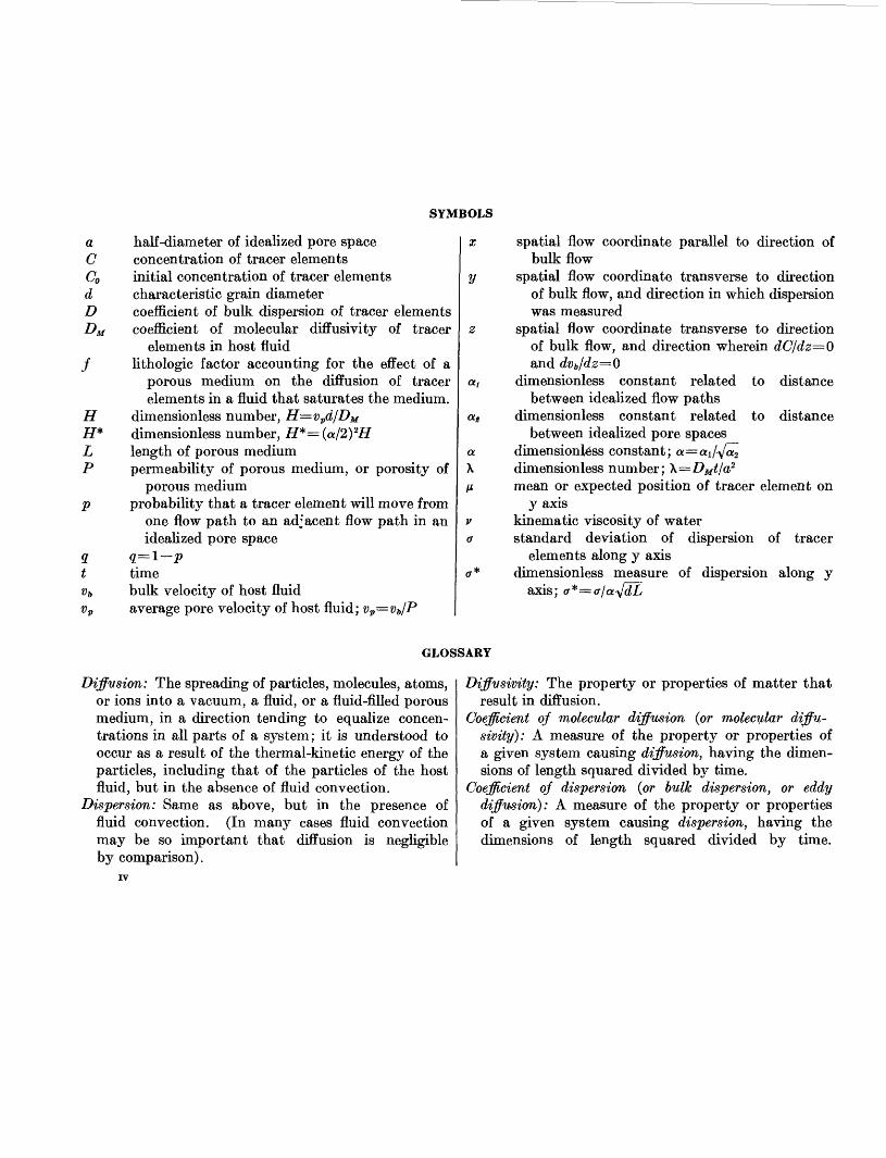
SYMBOLS
a CCod D
f
H H* L P
P
half-diameter of idealized pore spaceconcentration of tracer elementsinitial concentration of tracer elementscharacteristic grain diametercoefficient of bulk dispersion of tracer elementscoefficient of molecular diffusivity of tracer
elements in host fluid lithologic factor accounting for the effect of a
porous medium on the diffusion of tracerelements in a fluid that saturates the medium,
dimensionless number, H=vpd/DM dimensionless number, H*=(a/2)2H length of porous medium permeability of porous medium, or porosity of
porous medium probability that a tracer element will move from
one flow path to an adjacent flow path in anidealized pore space
q=l p timebulk velocity of host fluid average pore velocity of host fluid; vp =vb/P
x spatial flow coordinate parallel to direction ofbulk flow
y spatial flow coordinate transverse to directionof bulk flow, and direction in which dispersionwas measured
z spatial flow coordinate transverse to directionof bulk flow, and direction wherein dC/dz=Qand dvt,/dz=0
at dimensionless constant related to distancebetween idealized flow paths
otg dimensionless constant related to distancebetween idealized pore spaces_
a dimensiom^ss constant; a=a1 /A/a2 X dimensionless number; \=DMt/a2 H mean or expected position of tracer element on
y axisv kinematic viscosity of water a standard deviation of dispersion of tracer
elements along y axis <r* dimensionless measure of dispersion along y
axis <r* = <r
GLOSSARY
Diffusion: The spreading of particles, molecules, atoms, or ions into a vacuum, a fluid, or a fluid-filled porous medium, in a direction tending to equalize concen trations in all parts of a system; it is understood to occur as a result of the thermal-kinetic energy of the particles, including that of the particles of the host fluid, but in the absence of fluid convection.
Dispersion: Same as above, but in the presence of fluid convection. (In many cases fluid convection may be so important that diffusion is negligible by comparison).
Diffvsivity: The property or properties of matter that result in diffusion.
Coefficient of molecular diffusion (or molecular diffu sivity): A measure of the property or properties of a given system causing diffusion, having the dimen sions of length squared divided by time.
Coefficient of dispersion (or bulk dispersion, or eddy diffusion): A measure of the property or properties of a given system causing dispersion, having the dimensions of length squared divided by time.

FLUID MOVEMENT IN EARTH MATERIALS
TRANSVERSE DISPERSION IN LIQUID FLOW THROUGH POROUS MEDIA
BY EUGENE S. SIMPSON
ABSTRACT
It is assumed that a line source of tracer elements exists in a porous medium through which an incompressible fluid is flowing. Each tracer element is assumed (a) to be completely miscible in the fluid, (b) to be unaffected by the solid medium or by any other tracer element, and (c) to have a path dependent both on the motion of the fluid and on its own molecular diffusivity. As the tracer elements move away from the source they will disperse. A mathematical model, describing the dispersion transverse to the direction of bulk flow, is formulated under the following assumptions: (a) each path has an average direction parallel to the direction of bulk flow, herein termed "zero circuity"; and (b) tracer elements may transfer from one flow path to another by virtue of the molecular diffusivity of the elements. It is then found that the standard deviation of the dispersion is proportional to the square root of the product of grain size, length of flow, and probability that a tracer element will transfer from one flow line to another in a given unit distance. An estimate of the proba bility is obtained by equating it to that fraction of a large number of tracer elements that would diffuse across the centerline of an idealized pore space. The fraction will depend on (a) size of pore space; (b) velocity of fluid; and (c) coefficient of diffusivity of tracer elements.
A curve is plotted giving the relation between a dimensionless parameter, tr*, which is a measure of the dispersion in a given medium, and a dimensionless parameter, H*, which is a measure of fluid velocity and tracer-element diffusivity in the same medium. It is predicted that, within the range of Darcy's law, as velocity increases dispersion decreases.
A series of laboratory experiments designed to measure transverse dispersion in a relatively uniform medium, and per formed in the range of Reynolds number from 0.04 (approx) to 1.0 (approx), showed that as velocity increased dispersion decreased. The measured standard deviation of the dispersion ranged from 1.57 cm to 0.89 cm (with some scatter) in a bulk- flow distance of 119 cm, and the individual concentration distributions were found to be normal except near the end points.
Experimental data were reduced to dimensionless form by the assigning of an arbitrary but reasonable value to a dimensionless constant, and in this way the measured dispersion is found to be roughly double that predicted by theory. By analysis of other possible mechanisms of dispersion one concludes that the observed dispersion is best explained by assuming that a velocity- dependent dispersion (as predicted by theory) is superposed on a constant dispersion, independent of velocity, which results from wandering of stream paths (that is, nonzero circuity).
Finally, it is shown that at very low fluid velocity (R<0.005 for the experimental porous medium) the effect of molecular
diffusivity of the tracer elements overshadows the effects of other possible mechanisms causing dispersion. However, it is believed that dispersion caused by nonzero circuity increases with nonuniformity of the medium. The experimental medium was relatively uniform; hence, the relation between nonzero circuity and nonuniformity of the medium (as it occurs in most natural aquifers) remains to be investigated.
INTRODUCTION
Recent theoretical and experimental work on the mechanics of dispersion in liquid flow through porous media (Rifai and others 1956, p. 100) recognizes that the molecular diffusivity of tracer ions or of tracer particles does have an effect on dispersion. The im portance of this effect, however, was considered to be relatively slight except at very low fluid velocity and generally was ignored in the analysis of experimental data. The data so treated, almost without exception, pertained to longitudinal dispersion (dispersion paral lel to the direction of bulk flow), and the experiments were performed in tubular columns of sand or beads. In this kind of dispersion the effect of molecular dif fusivity undoubtedly is small, but the flow conditions, particularly in nature, under which it is small enough to be neglected remain to be identified.
In the case of transverse dispersion (dispersion per pendicular to the direction of bulk flow) different mechanisms are'mvolved, and it is not at all permissible to ignore molecular diffusivity. In the longitudinal case the mechanisms related to dispersion are (1) fluid- velocity gradients within the individual pore spaces,(2) variations in length of individual flow paths, and(3) molecular diffusivity of tracer ions. In the trans verse case the mechanisms seem to be (1) the inter twining or "wandering" of flow paths and (2) the molecular diffusivity of tracer ions. Within the realm of Darcy's law the intertwining-paths mechanism is independent of velocity and may be treated analytically by use of a random-walk model or some modification thereof (Scheidegger, 1958). The molecular-diffusivity mechanism, however, is dependent on flow velocity.
C-l

C-2 FLUID MOVEMENT IN EARTH MATERIALS
Most analyses of transverse dispersion that have appeared in the literature indicate that the flow-path mechanism is thought much more important than molecular diffusivity, particularly in the upper range of flow velocities that accord with Darcy's law. Beran, 1 for example, gives a rough estimate, based on mathe matical analysis alone, of the range in which diffusivity may be neglected entirely. On the other hand, C. V. Theis of the U.S. Geological Survey, in various discus sions and in unpublished memoranda, has proposed an opposite view; that is, that for uniform media diffusivity is the more important mechanism and that intertwining of flow paths either does not exist or is so minor that it may be neglected. Theis points out that the dis tances separating individual flow paths within pore spaces are so small that there is ample time available, even at velocities in the upper range of Darcy's law, for tracer ions to diffuse from one flow path to another.
For this study I devised a mathematical model for transverse dispersion based on the mechanism of molec ular diffusivity, and tested the validity of the math ematical analysis by experiments designed for that purpose. So far as I know, these laboratory experi ments are the first of their kind, except for those per formed by Kitagawa (1934) in Japan. Kitagawa used a salt solution as tracer in a horizontal bed of sand and made no allowance for possible density effects. He also averaged the results of 15 individual experimental runs, each having significant differences from the others in distribution of concentration and in position of mean value. He then used the average distribution to compute the standard deviation of the dispersion. Consequently, his measurement was more than 20 times larger than mine. No other laboratory data seem to be available with which results might be compared.
ACKNOWLEDGMENTS
The theoretical investigation and the experiments described in this report were carried out at Columbia University in New York, 1957-58, under the sponsor ship of the U.S. Geological Survey, at a time when I was a graduate student in the Department of Geology. Prof. Richard Skalak, Sidney Paige, and A. N. Strahler acted as advisors. Throughout the course of the work these men gave freely of their time for discussion and counsel. In addition, I had the advantage of many helpful discussions with various colleagues in the Geo logical Survey, in particular with C. V. Theis, R. R. Bennett, Wallace de Laguna, and H. E. Skibitzke. De Laguna also suggested the tracer dye. used in the experiments. S. K. Aditya of the Chemical Engineer-
1 Beran, M. J., 1955, Dispersion of soluble matter in slowly moving fluids: doctoral dissertation, Harvard Univ., p. 4:12.
ing Department of the university kindly permitted the use of his laboratory for the measurement of molecular diffusivity of the tracer solution and helped in other ways.
THEORETICAL ANALYSIS
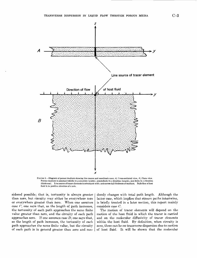
An analysis is made of the transverse dispersion from a continuous line source of tracer elements dissolved or suspended in a host fluid that flows through a porous medium. The length and breadth of the medium are large compared to its thickness (fig. 1). For this purpose a tracer element is defined as an identifiable ion, or molecule, or colloidal particle, dissolved or sus pended in the host fluid; a fluid element is defined as a "point volume" of the host fluid whose diameter is small compared to the pore diameter of the porous medium, but large compared to molecular dimensions. The line source is considered to extend along the z axis across the full thickness of the medium, and the tracer elements enter the host fluid in such manner as to cause no change in its velocity field. The direction of bulk flow of the host fluid is parallel to the positive direction of the x axis. There is no bulk flow in either the y or the z direction, because the fluid is incompres sible and the medium is homogeneous and of constant thickness, and there is no flow across the boundaries of the medium except in the x direction. It is assumed that motion of any tracer element in the z direction will be compensated for by an equal and opposite motion of some other element; hence, there is no change in concentration in the z direction. It is assumed also that steady-state motion of both host fluid and tracer elements is established. Under these conditions the concentration distribution of the tracer elements may be discribed in terms of the space coordinates x and y. It is the present purpose to describe transverse disper sion only that is, dispersion in the y direction, in terms of distance from origin, fluid velocity, diffusivity of tracer elements, grain diameter and porosity of medium, and certain dimensionless numbers related to the geometry of the medium.
It is useful now to define conceptually two character istics of a flow path: tortuosity and circuity. Tortu osity is a measure of the wiggles in a flow path and is the difference between the real length of flow path and the straight-line length per unit length of bulk flow. Circuity is a measure of the difference between the average direction of an individual flow path and the direction of bulk flow (see fig. 2). Both tortuosity and circuity are measured over distances that are large compared to grain size.
In a disordered porous medium, such as may be obtained with randomly packed, irregularly shaped grains of sand, only cases C and D of figure 2 are con-
TRANSVERSE DISPERSION IN LIQUID FLOW THROUGH POROUS MEDIA C-3
Line source of tracer element
^i
FIGURE 1. Diagram of porous medium showing line source and coordinate axes; A, Cross-sectional view, B, Plane view. Porous medium is assumed infinite in y direction (width), semiinfinite in x direction (length), and finite in ? direction (thickness). Line source of tracer elements is coincident with z axis across full thickness of medium. Bulk flow of host fluid is in positive direction of x axis.
sidered possible; that is, tortuosity is always greater than zero, but circuity may either be everywhere zero or everywhere greater than zero. When one assumes case C, one says that, as the length of path increases, the tortuosity of each path approaches the same finite value greater than zero, and the circuity of each path approaches zero. If one assumes case D, one says that, as the length of path increases, the tortuosity of each path approaches the same finite value, but the circuity of each path is in general greater than zero and ran
domly changes with total path length. Although the latter case, which implies that stream paths intertwine, is briefly treated in a later section, this report mainly considers case C.
The motion of tracer elements will depend on the motion of the host fluid in which the tracer is carried and on the molecular diffusivity of tracer elements within the host fluid. By definition, when circuity is zero, there can be no transverse dispersion due to motion of host fluid. It will be shown that the molecular
C-4 FLUID MOVEMENT IN EARTH MATERIALS
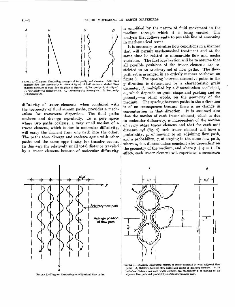
FIGURE 2. Diagram illustrating concepts of tortuosity and circuity. Solid lines indicate flow (not necessarily in plane of flgure) of fluid elements; dashed lines indicate direction of bulk flow (in plane of flgure). A, Tortuosity=0; circuity=0. P, Tortuosity=0; circuity=>0. C, Tortuosity>0; circuity=0. D, Tortuosity >0; circuity>0.
diffusivity of tracer elements, when combined with the tortuosity of fluid stream paths, provides a mech anism for transverse dispersion. The fluid paths coalesce and diverge repeatedly. In a pore space where two paths coalesce, a very small motion of a tracer element, which is due to molecular diffusivity, will carry the element from one path into the other. The paths then diverge and coalesce again with other paths and the same opportunity for transfer occurs. In this way the relatively small total distance traveled by a tracer element because of molecular diffusivity
< I Arbitrary flow path
.Average positionof flow path
\ x
FIGUBE 3. Diagram illustrating set of idealized flow paths.
is amplified by the nature of fluid movement in the medium through which it is being carried. The analysis that follows seeks to put this line of reasoning in mathematical terms.
It is necessary to idealize flow conditions in a manner that will permit mathematical treatment and at the same time be related to measurable flow and media variables. The first idealization will be to assume that all possible positions of the tracer elements are re stricted to an arbitrary set of flow paths. The flow- path set is arranged in an orderly manner as shown on figure 3. The spacing between successive paths in the y direction is determined by a characteristic grain diameter, d, multiplied by a dimensionless coefficient, ax , which depends on gram shape and packing and on porosity in other words, on the geometry of the medium. The spacing between paths in the z direction is of no consequence because there is no change in concentration hi that direction. It is assumed also that the motion of each tracer element, which is due to molecular diffusivity, is independent of the motion of every other tracer element and that for each unit distance a2d (fig. 4) each tracer element will have a probability, p, of moving to an adjoining flow path, and a probability, g, of staying in the same flow path, where «2 is a dimensionless constant also depending on the geometry of the medium, and where p + 2 = 1. In effect, each tracer element will experience a succession
FIGURE 4. Diagram illustrating motion of tracer elements between adjacent flow paths. A, Relation between flow paths and grains of idealized medium. B, In bulk-flow distance aid each tracer element has probability p of moving to an adjacent flow path and probability g of staying in same path.
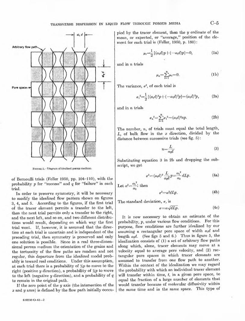
TRANSVERSE DISPERSION IN LIQUID FLOW THROUGH POROUS MEDIA C-5
Arbitrary flow path
Pore space-?-
\ /
FIGTJKE 5. Diagram of idealized porous medium.
of Bernoulli trials (Feller 1950, pp. 104-110), with the probability p for "success" and g for "failure" in each trial.
In order to preserve symmetry, it will be necessary to modify the idealized flow pattern shown on figures 3, 4, and 5. According to the figures, if the first trial of the tracer element permits a transfer to the left, then the next trial permits only a transfer to the right, and the next left, and so on, and two different distribu tions would result, depending on which way the first trial went. If, however, it is assumed that the direc tion at each trial is uncertain and is independent of the preceding trial, then symmetry is preserved and only one solution is possible. Since in a real three-dimen sional porous medium the orientation of the grains and the tortuosity of the flow paths are random and not regular, this departure from the idealized model prob ably is toward real conditions. Under this assumption, at each trial there is a probability of %p to move to the right (positive y direction), a probability of %p to move to the left (negative y direction), and a probability of q to remain in the original path.
If the zero point of the y axis (the intersection of the x and y axes) is defined by the flow path initially occcu-
pied by the tracer element, then the y ordinate of the mean, or expected, or "average," position of the ele ment for each trial is (Feller, 1950, p. 180):
=0,
and in n trials
The variance, <r2, of each trial is
and in n trials
(la)
(Ib)
(2a)
(2b)
The number, n, of trials must equal the total length, L, of bulk flow in the x direction, divided by the distance between successive trials (see fig. 5):
(3)
Substituting equation 3 in 2b and dropping the sub script, we get
a2
Let c?=-^-} then
The standard deviation, <r, is
(4a)
(4b)
(4c)
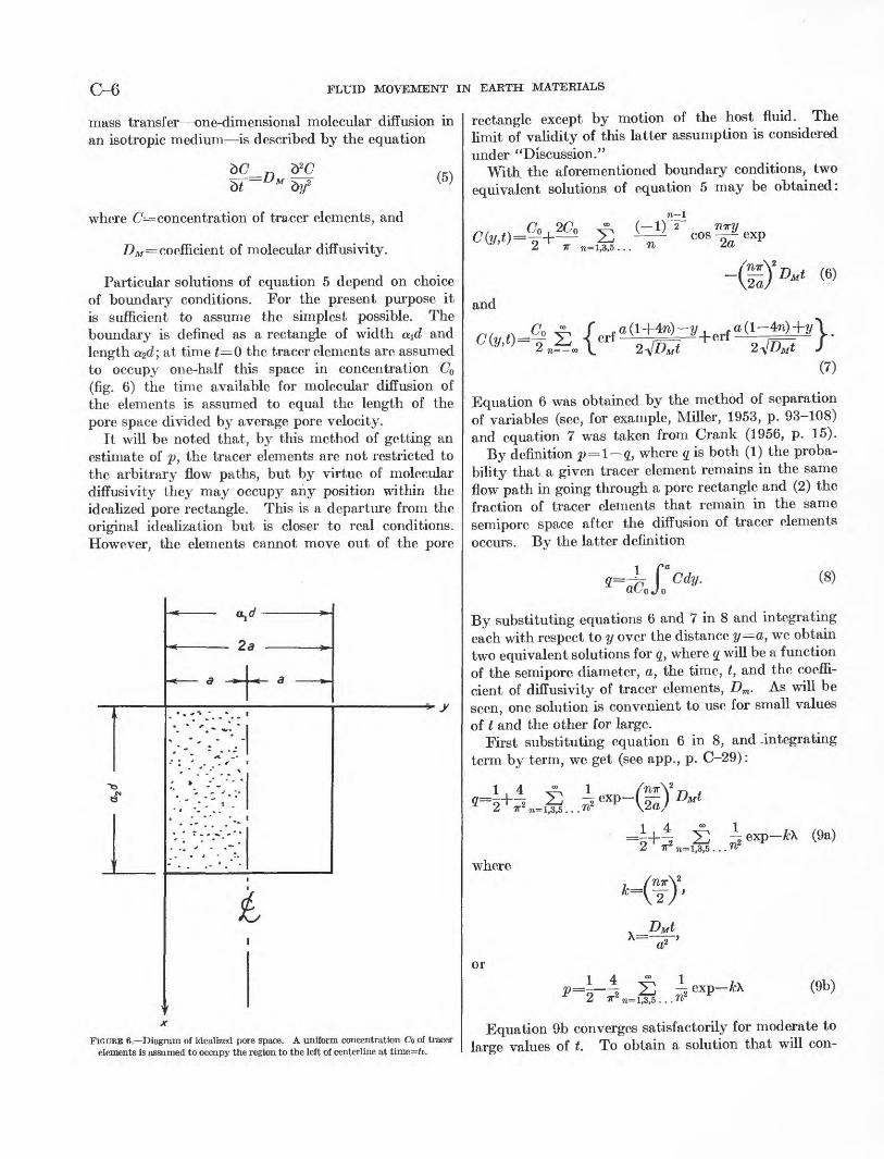
It is now necessary to obtain an estimate of the probability, p, under various flow conditions. For this purpose, flow conditions are further idealized by our assuming a rectangular pore space of width ^d and length a2d. (See figs 5 and 6.; Thus in figure 5, the idealization consists of (1) a set of arbitrary flow paths along which, alone, tracer elements may move at a velocity equal to average pore velocity, and (2) rec tangular pore spaces in which tracer elements are assumed to transfer from one flow path to another. Within the context of the idealization we may regard the probability with which an individual tracer element will transfer within time, t, in a given pore space, to equal the fraction of a large number of elements that would transfer because of molecular diffusivity within the same time and in the same space. This type of
618550O-62 2
C-6 FLUID MOVEMENT IN EARTH MATERIALS
mass transfer one-dimensional molecular diffusion in an isotropic medium is described by the equation
where C= concentration of tracer elements, and
DM= coefficient of molecular diffusivity.
Particular solutions of equation 5 depend on choice of boundary conditions. For the present purpose it is sufficient to assume the simplest possible. The boundary is defined as a rectangle of width aid and length a2d; at time t=G the tracer elements are assumed to occupy one-half this space in concentration C0 (fig. 6) the time available for molecular diffusion of the elements is assumed to equal the length of the pore space divided by average pore velocity.
It will be noted that, by this method of getting an estimate of p, the tracer elements are not restricted to the arbitrary flow paths, but by virtue of molecular diffusivity they may occupy any position within the idealized pore rectangle. This is a departure from the original idealization but is closer to real conditions. However, the elements cannot move out of the pore
2a
*" y
FIGURE 6 Diagram of idealized pore space. A uniform concentration Co of tracer elements is assumed to occupy the region to the left of centerline at time=<o.
rectangle except by motion of the host fluid. The limit of validity of this latter assumption is considered under "Discussion."
With the aforementioned boundary conditions, two equivalent solutions of equation 5 may be obtained:
n-l(-i)-r mry cos-^ exp
and
(7)
Equation 6 was obtained by the method of separation of variables (see, for example, Miller, 1953, p. 93-108) and equation 7 was taken from Crank (1956, p. 15).
By definition p=l & where g is both (1) the proba bility that a given tracer element remains in the same flow path in going through a pore rectangle and (2) the fraction of tracer elements that remain in the same semipore space after the diffusion of tracer elements occurs. By the latter definition
2=77T (8)
By substituting equations 6 and 7 in 8 and integrating each with respect to y over the distance y=a,v?e obtain two equivalent solutions for g, where g will be a function of the semipore diameter, a, the time, t, and the coeffi cient of diffusivity of tracer elements, Dm . As will be seen, one solution is convenient to use for small values of t and the other for large.
First substituting equation 6 in 8, and-integrating term by term, we get (see app., p. C-29):
-; exD I ^ I Z?M<
+4 ±12 7T OT = 1,3,5.
exp-ArX (9a)
where
,A=
DMt
or
(9b)
Equation 9b converges satisfactorily for moderate to large values of t. To obtain a solution that will con-

TRANSVERSE DISPERSION IN LIQUID FLOW THROUGH POROUS MEDIA C-7
verge satisfactorily for small values of t, we use 7 in conjunction with 8 and obtain the following (see app., p. C-29).
- C (. |(exp
+(10a)
where X= ̂ - as before. a2
To a very close approximation, when XfSO.Ol, equation lOa simplifies to
and
By figure 5
2=1 »/-= 1-0.5642 Vx>
V*
(lOb)
(lOc)
(Ha)
where VP = average pore velocity v6 = average bulk velocity
= PvP, where P = porosity of medium.
By figure 6
(lib)
and
X=DMt
wherea2
2
or
a2= as in equation 4,<X2
=i=( £ ) H
where(12b)
(12c)
2 To my knowledge, the dimensionless number H was first explicitly used in flow through porous media by Beran (see footnote 1, p. C-2), although Taylor (1953, p. 190) used it implicitl y in his treatment of dispersion in flow through tubes. It is analogous to the Peclet number (Pai, 1956, p. 98) In which thermal diffusivity replaces molecular diffusivity. The H number is derivable also by dimensional analysis.
By equation 4c
and by 9b and lOc p is a known function of X. Hence, a curve can be plotted giving the relation between the dimensionless parameter (T/o/-\fdL} which is a measure of dispersion in a given medium, and the dimensionless
parameter ( ~ YH, which is a measure of fluid velocity
and tracer-element diffusivity through the same medium. The relation between q and 1/X as computed by means of 9a and lOb is shown on figure 7. Finally, figure 8 shows the relation between 1/X and a
DESCRIPTION OF APPARATUS AND EXPERIMENTAL PROCEDURE
The name given to the principal apparatus herein described is "dispersometer." Additional apparatus also was built to supply de-aired water. For purposes of description the dispersometer may be separated into three parts: (A) reservoirs and overflow (constant- head) tanks to provide water and tracer solution at constant head, (B) porous block (and associated flow controls) through which the fluid moves and in which the dispersion takes place, and (C) connections for taking samples and measuring flow gradiant and dis charge. The apparatus is shown in the following illustrations: figure 9 is a diagram showing the arrange ment of the various parts; figure 10 is a drawing of the porous block; figure 11 is a diagram of the apparatus to supply de-aired water; and figure 12 is a photograph of the assembled apparatus.
Measurements of dispersion were made at various flow velocities. Each dispersion measurement made at a given flow velocity and involving all the following steps is referred to as a "run." In the tabulation of data (table 1, next section) runs are consecutively numbered.
Measuring dispersions, or runs
1. The two overhead reservoirs were filled with de-aired water and allowed to stand for at least 24 hours to permit equal ization of temperatures.
2. Indigo carmine dye, used as a tracer, was dissolved in one reservoir in the proportion of 50 parts per million (ppm) for the first 5 runs and 20 ppm for the remaining 8 runs.
3. The constant-head overflow tanks were adjusted to provide the desired head. The clamps controlling discharge from the overhead reservoirs into the overflow tanks were opened and then clamps between overflow tanks and porous block were opened.
4. Discharge was maintained through the porous block until steady-state conditions were attained with respect to dispersion. The time necessary for this was estimated by calculation but determined by visual inspection of the dye front as it moved through the block. The block was

C-8 FLUID MOVEMENT IN EARTH MATERIALS
1.0 I
0.8
0.6
0.4
0.2
o.i 0.5 1.0 5.0 10 50 100 500 1000 5000 10,000
FIGURE 7. Graph of probability q plotted against -
1.0
0.8
OT6
0.4
0.2
0.1 0.5 1.0 5.0 10 50 100 500 1000
FIGURE 8. Graph of - -<JdL plotted against ;:
5000 10,000

TRANSVERSE DISPERSION IN LIQUID FLOW THROUGH POROUS MEDIA C-9
>»Q. Q.3OTk_
1i1?£
11
^ ^
Overhead
s4 : )
reservoir, Overheawater plus dye tracer v
7?/////////////
i
"80)
i
i
*
8£* ^
x/1/1/
,
^^^^B ^^^^H
/////S/////////S //////////////s
1 I x
''
y^ >.
/ /// /7/y/
L funnels
To waste To w
_ r>ie-^KorrTA erwMitc
water
////////////x
/////> /
To wa
Flow-d cha
'SSS
^-^
ste
:5
"Adjusta ft
Discha (not
Manometer tubes/ /
!/ \/
stribution^. mbers
s+s*tfyf:::f.
;: ;'.> ;
'.' ' ".
[v.v/:
;£y;';
r-'-v-:
1
'Constant-head tank
/
><
FIGURE 9. Flow diagram of dispersometer.

C-10 FLUID MOVEMENT IN EARTH MATERIALS
. Holes connected to tubuldr rubber discharge spouts
Upper flow-separation plates, 23 in all
Note: Lucite frame not shown
Water in
Water plus dye tracer in
FIGURE 10. Diagram of porous block.

TRANSVERSE DISPERSION IN LIQUID FLOW THROUGH POROUS MEDIA C-ll
To waste
Low-pressure steam in
Copper tubing 50 ft by Vz inch
T i I f f f f i//r/rf/i/tf / f f r / f ft f //
il 111 f
To water reservoirs
FIGURE 11. Diagram of apparatus to supply de-aired water.
mounted vertically; flow entered at the bottom and dis charged at the top through a series of horizontal spouts.
5. After steady-state dispersion was established, the rack of test tubes was inserted under the discharge spouts to obtain a sample suite from all spouts simultaneously. Either 2 or 3 such suites were sampled per run, at intervals of 1 to 2 hours.
6. Total rate of discharge of fluid was measured; it together with manometer readings of flow gradient and known dimensions of the porous block, permitted calculation of permeability and bulk-flow velocity. The rate was meas ured several times during each run. Temperature of in fluent and effluent fluid also was measured.
7. Relative concentration of dye in each test tube was deter mined colorimetrically.
The rate of discharge from each spout could be regulated by raising or lowering the high point of a rubber discharge tube. Each discharge tube had a hole cut at its high point to break suction. At the beginning of each run the tubes were adjusted as required to make the discharge through each proportional to the cross-sec tional area of the porous block that the tube drained (tubes near the centerline of the block were on 0.75 cm centers, whereas tubes farther out were on wider centers; see fig. 10). For runs at relatively high velocities this
was easily accomplished, but for runs at low velocities precise adjustment was not possible, presumably be cause surface-tension forces within the tubes were large enough compared with other forces to affect discharge. The possible effect on dispersion of this non-uniformity of discharge will be discussed later.
For each run 2 or 3 suites of samples were obtained in 50-ml test tubes. Each suite contained 24 samples. It was early determined that only the nearest 4 or 5 samples on each side of the interface between the dye solution and the water needed measurement. The con centration change, if any, in the others could not be detected. The procedure in measuring the distribution of concentration in each suite of samples was as follows:
Measuring distribution of concentration
1. The sample on the dye side farthest from the interface was considered to contain the original dye concentration C= C0 . (The concentration of this sample and that of the overhead reservoir should, perhaps, have been identical but there usually was a very small, unexplained, difference.) Simi larly, the sample on the water side farthest from the inter face was considered to contain the original concentration C=0. By successive dilutions of one in the other, and

C-12 FLUID MOVEMENT EST EARTH MATERIALS
-, '*vSo m pie. I rock
FIGUHE 12. Photograph of dispersometer, front view.
measuring each in the colorimeter, a rating curve of relative concentration C/C0 plotted against colorimeter reading was obtained.
2. Colorimeter readings were then taken of the samples of un known concentration and converted into relative concen tration by means of the rating curve.
3. The relative concentrations of the samples in each suite were plotted on arithmetic probability paper, and the value of the standard deviation of the dispersion was obtained graphically (figs. 14-26).
Measuring the concentration of dilute dye solutions with a colorimeter turned out to be more time consum ing than had been expected. So-called precision pyrex tubes had to be carefully matched and positioned for each suite of measurements, and frequent checks against the standard solution had to be made to avoid errors due to drift of the instrument.
The coefficient of thermal diffusivity of the indigo carmine dye was measured by following the procedure described by McBain and Liu (1931). A dye solution of 20 ppm by weight in distilled water was placed in the upper cell of the diffusion apparatus, and distilled water was placed in the lower cell. The two cells were separated by a sintered-glass membrane.
After 3 days 19 hours at 20 °C the liquids were withdrawn and the relative concentration in each cell was measured. A calculation based on the concen tration in the lower cell gave a coefficient DM=Q.57 X10~ 5 cm2/sec, and a calculation based on the concen tration in the upper cell gave DM=Q.67 X 10~s cm2/sec. For purposes of calculation in this report the coefficient will be taken as DM=O.G2 x 10~5 cm2/sec.
A photospectrogram of the dye solution (20 ppm by weight) was obtained and is shown in figure 13.
1.5
i.o
0.5
2000 4000 WAVELENGTH, A
6000
FIGUBE 13. Photospectrograph of tracer solution. Tracer solution consisted of indigo carmine dye in de-aired water, 20 ppm by weight.
The porous block deserves special mention. It was made by mixing an epoxy resin with crushed quartz. The quartz grams were angular, with sharp edges, and some were platy or rod shaped. Sieving for 10 minutes in a ro-tap machine resulted in the size dis tribution shown on figure 14. As indicated by this figure, the sieve diameter of about 95 percent of the grains was between 0.40 mm and 0.60 mm, and by inspection 0.48 mm is taken to be average. For pur poses of calculation in this report, a characteristic grain diameter of d=OA8 mm will be used.
The resin-sand mix was prepared in batches in the proportion of 2 parts resin plus hardener to 98 parts crushed quartz by weight. First the resin and hardener were mixed together in a container; then the quartz was added slowly and thoroughly stirred into the resin. The finished mixture had the appearance and feel of a damp beach sand. The batch then was poured into the plexiglass frame and vibrated into place to get maximum density and uniformity. The vibrator con-

TRANSVERSE DISPERSION IN LIQUID FLOW THROUGH POROUS MEDIA C-13
100
80
ICJ I-Z
az60
20
0.03 0.04 0.05 SIEVE OPENING, IN CENTIMETERS
0.06 0.07
FIGURE 14. Mechanical analysis of sand used in porous block.
sisted of a tamp-rod attached to a commercial Vibro- tool. Unfortunately the batch method resulted in horizontal zones of contact that could be visually identified. The porosity of the finished block was computed to be 0.37, on the basis of measured volume of the plexiglass container and computed volume (based on measured weight and specific gravity) of the sand and resin.
The advantages of a porous block cast in a plexiglass frame over a medium of nonbonded grains are that (1) permeability of the block is constant or nearly so, whereas permeability of nonbonded grains tends to decrease with time and with use, presumably because grains continue to settle; (2) the porous block may be drilled at any place for manometer connections and other needs, whereas for nonbonded grains special' connections must be machined into the container at the time of fabrication; and (3) a wire-mesh support for the porous block is unnecessary. The chief dis advantage of a porous block (and this is not an inherent feature) appears to be the "bedding planes" where one batch is in contact with the next. However, these planes are in themselves quite uniform and are at right angles to the flow direction and should not affect the validity of the dispersion measurements.
De-aired water was obtained in the following manner (fig. 11): (1) low-pressure steam from a vent supply in the laboratory was directed through a 50-foot coil of K-inch copper tubing; (2) the tubing was immersed in a bath of cold water which caused the steam to con dense and cool; (3) the resulting water contained air which showed up in large bubbles; (4) the water plus air-bubble mixture was fed into the midsection of a standpipe; the standpipe was open at the top and virtually all the air with some water rose to the top of the pipe and overflowed to waste; (5) the remainder of the water was withdrawn from the base of the pipe and discharged into the dispersometer reservoirs. Samples of the de-aired water were examined for air content by slow heating in a closed vessel provided with an expansion tube. Tiny air bubbles began to appear only after water temperature exceeded 90°C, and these bubbles redissolved when the sample was cooled. Apparently, a little air was dissolved by the condensed steam in the time required for it to flow through the coil and into the standpipe. The de-aired water system was operated as required to fill the overhead reservoirs before each run.
EXPERIMENTAL RESULTS
Thirteen runs were made in accordance with the procedures outlined in the previous section. The distribution of concentration for the several suites of each of the 13 runs is plotted on arithmetic probability paper, figures 15 through 27. When so plotted the points of each suite fall on a straight line, except for the extreme end points. Hence, to a close approxi mation the distribution of concentration in each suite is normal. That is, the concentration distribution in each case is defined by the following equation
where, <r= standard deviation of distribution,m=distance to mean value; that is, where C/C0 = %, y= distance to value C/C0.
If, in each case, the origin of coordinates is placed at the mean value, then m=0 and equation 14 becomes
618550 O-62 3

C-14 FLUID MOVEMENT IN EARTH MATERIALS
99.99 99.9 90 80 70 60 50 40 30 20 C/C0 , IN PERCENT
10 0.1 0.01
FIGURE 15. Concentration distribution, run 1, suites A, B, and C.
99.99 99.9 99 90 80 70 60 50 40 30 20 C/C0 , IN PERCENT
10 0.01
FIGURE 16. Concentration distribution, run 2, suites A, B, and C.

TRANSVERSE DISPERSION IN LIQUID FLOW THROUGH POROUS MEDIA C-15
17
16
15
14
13
12
10
99.99 99.9 99 90 80 70 60 50 40 30 20 , IN PERCENT
10 0.1 0.01
FIGUEE 17. Concentration distribution, run 3, suites A, B, and C.
20
19
18
B
16
15
A
Xl
14
13
~^~
1299.99 99.9 99 90 80 70 60 50 40 30 20 10
C/C0 , IN PERCENT
FIGURE 18. Concentration distribution, run 4, suite^ A, and B.
0.1 0.01

C-16 FLUID MOVEMENT IN EARTH MATERIALS
19
18
17
16
B
15
14
13
12
99.99 99.9 99 90 80 70 60 50 40 30 20 C/C0 , IN PERCENT
10 0.1 0.01
FIGTJKE 19. Concentration distribution, run 5, suites A and B.
16
15
14
13
10
99.99 99.9 99 90 80 70 60 50 40 30 C/Ca , IN PERCENT
20 10 0.1 0.01
FIGTJKE 20. Concentration distribution, run 6, suites A and B.

TRANSVERSE DISPERSION IN LIQUID FLOW THROUGH POROUS MEDIA C-17
12
99.99 99.9 90 80 70 60 50 40 30 20 CIC0 , IN PERCENT
10 0.1 0.01
FIGURE 21. Concentration distribution, run 7, suites A and P.
18
17
16
15
\
14
13
\
12
11
10
\
99.99 99.9 99 90 80 70 60 50 40 30 20 10 C/C0 , IN PERCENT
0.1 0.01
FIGURE 22. Concentration distribution, run 8, suites A, B, and C.

C-18 FLUID MOVEMENT IN EARTH MATERIALS
18
17
16
15
14
13
N
12
11
99.99 99.9 99 90 80 70 60 50 40 30 20 CIC0 , IN PERCENT
10
FIGURE 23. Concentration distribution, run 9, suites A and B.
0.1 0.01
17
16
15
14
13
12
11
10
99.99 99.9 99 90 80 70 60 50 40 30 20 C/CD , IN PERCENT
10 0.1 0.01
FIGUBE 24. Concentration distribution, run 10, suites A and Ji.

TRANSVERSE DISPERSION IN LIQUID FLOW THROUGH POROUS MEDIA C-19
18
17
16
\
14
13
12
99.99 99.9 99 90 80 70 60 50 40 30 20 C/Co, IN PERCENT
10
FIGURE 25. Concentration distribution, run 11, suites A, fi, and C.
0.1 0.01
17
16
15
« S3
i-12
10
99.99 99.9 99 90 80 70 60 50 40 30 20 10 C/C0 , IN PERCENT
0.1 0.01
FIGURE 26. Concentration distribution, run 12, suites A, fi, and C.

C-20 FLUID MOVEMENT IN EARTH MATERIALS
15
14
13
12
10
99.99 99.9 99 90 80 70 60 50 40 30 20 C/C0 ,IN PERCENT
10 0.1 0.01
FIGURE 27. Concentration distribution, run 13, suites A and B.
According to the geometry of the experiment (fig. 10) the mean value should occur midway between spouts 12 and 13. Actually, the mean value (the interface between dye solution and water) tended to migrate sideways slightly during the course of each run. Also, the vertical line of the interface as seen through the lucite frame was not perfectly straight but was gently sinuous. However, the sinuousity was fixed and was the same at all velocities. Therefore, it can be pre sumed to have resulted from a nonuniformity of the medium and did not represent an instability in the flow field.
The migration of the interface probably resulted from a nonuniform, gradually increasing resistance to flow at the base of the porous block that occurred during the course of each run. This, in turn, probably was caused by the presence of fine lintlike sediment found suspended in the feed fluids. As the fluids moved through the block, this sediment must have become trapped in the pores of its base. (The concentration of the sediment was low and its presence was not noted until the experiments were well under way. No remedial measures were taken.) In any case, it was found that the position of the interface could be changed at will; that is, it could be made to migrate laterally simply by varying the entrance-head relation
ship between water and dye solution. Except for the first few runs which were begun with entrance heads equal, the heads were adjusted to put the interface reasonably close to the centerline of the block. The possible effect, if any, on test results of interface migration will be discussed farther on.
As was noted, the extreme end points of the con centration distribution curve do not, in general, fall on the straight lines of figures 15 and 26. There are various possible explanations for this: (1) the colori- metric method of measuring concentration is less accurate for the extremes of any given range of con centrations than for the intermediate concentrations (the filters, light intensity, etc., were adjusted to pro vide full-scale deflection of the instrument for the range of concentrations measured). (2) According to the theory presented in this report, the distribution of the concentrations is binomial rather than normal. For distributions involving a large number of independent events, the normal and binomial distributions are practically identical, except that the limits of the binomial are finite, whereas those of the normal are infinite. On normal probability paper a normal dis tribution would plot as a straight line, whereas a binomial distribution would plot as a straight line except for the extreme values, which would tend to

TRANSVERSE DISPERSION IN LIQUID FLOW THROUGH POROUS MEDIA C-21
plot off the line in a direction away from the mean. This is seen to be the case for most of the extreme values plotted.
If, in spite of the slight deviations, the distributions are treated as normal, it becomes possible to measure the standard deviation, a, in each case from the straight-line plots. In a normal distribution at +0-, <7/<70=0.841, and at a, <7/<?0 =0.159. The concentra-
TABLE 1. Summary c
Time Veloc
Run Suite
1 1AIB1C
2 2A2B2C
3 3A3B3C
4 4A4B
5 5A5B
6 6A6B
7 7A7B
8 8A8B8C
9 9A9B
10 10A10B
11 11A11B11C
12 12A12B12C
13 13A13B
Date
1/22/58do.
1/24/58
1/30/58do.
1/31/58
2/3/58do.do.
2/10/58do.
2/11/58do.
2/14/58do.
2/19/58do.
2/26/58do.
8/27/58
3/12/58do.
3/19/58do.
3/28/58do.do.
4/3/58do.do.
4/30/58do.
Startof run
?
?
?
12:15Pdo.
11:30 A
12:30Pdo.do.
11:30Ado.
10:45Ado.
1:30Pdo.
11:40 Ado.
12:OONdo.
1:OOP
12:OONdo.
12:10Pdo.
11:OOAdo.do.
11:15Ado.do.
2:30Pdo.
1 Temperature shown is that ofnever more
2 Riilk VP
than a few
Innit.v J)ii=
tenths of a
OIA Pnrf
Suite Temoera-sampled ture i
4:OOP6 :OOP3:40P
3:30P5:OOP2:05P
3:25P4:50P7:40P
3:35P7:10P
1:10P2:30P
4:10P6:05P
2:40P4:15P
2:40P4:25P3:25P
2:OOP3:25P
2:30P4:05P
3:40P6:25P7:15P
3:35P5:OOP6:OOP
3:55P5:18P
influent water;degree different
> \7plni»it.v n _^=-
(°C)
262627
282827
252525
2424
2424
2424
2323
282827
2929
2828
292929
282828
2828
tion distributions are plotted against spout numbers. Hence, 2o- equals the distance (determined by the spout numbers and fractional distances thereof) between (7/^=0.841 and <7/<70 =0.159. The figures given in the final column of table 1 were obtained in this way. To evaluate the validity of these figures, it is necessary to attempt to identify and evaluate possible sources of error.
/ Experimental Results
ity'. Permeability* Coefficient of ..Standard?(cm per see)
V* vp
0. 0141 0. 0381.0139.0139
.0245.0244.0238
.0184
.0181
.0176
.00811. 00731
.0320
.0312
. 01365
.0128
. 0223
.0220
.0183
.0174
. 0164
.0605
.0594
.0324
.0316
. 00383. 00306. 00293
. 00387. 00327. 00322
. 0859
.0837
effluent water
Vb Vb
.0376.0376
.0663.0660.0644
.0497
.0489
.0476
.0219.0198
.0865
.0843
. 0369
.0346
.0603
.0595
.0495
.0470
.0443
. 164
. 160
.0875
.0855
. 01035. 00828. 00792
. 01045. 00884. 00870
. 232
. 226
Gradient *
0. 0655.0655.0645
. 114. 113. 112
.0900
.0885
.0880
.0427.0378
. 160
. 157
.0700. 0662
. 1170. 1153
.0858
.0812
.0785
. 291
. 286
. 162
. 157
.0185. 0146. 0140
.0202
.0172
.0168
. 3940
. 3835
5 Coefficient of
formula
(em per sec) Diffusi vitv n w >P,
0. 215 0.. 212. 216 .
. 215 .. 216 .. 212 .
. 204 .. 204 .. 200 .
. 190 .. 193 .
. 200 .. 199 .
. 195 .. 193 .
. 191 .. 191 .
. 213 .. 214 .. 209 .
. 208 .
. 208 .
. 200 .
. 201
. 207 .
. 209 .. 209 .
. 192 .. 190 .. 192 .
. 218 .
. 218 .
diffusivityT
DM=7fTD 'M where,1 20
Pjo (em* per sec)
19 0. 63X10~ 518 .6318 . 63
18 . 6418 .6418 .63
18 .6318 . 6318 . 63
17 . 6318 . 63
18 .6318 . 63
18 . 6318 . 63
18 .6318 .63
18 . 6418 . 6418 . 63
17 . 6417 . 64
17 . 6417 . 64
17 . 6417 .6417 .64
16 . 6416 . 6416 .64
18 . 6418 .64
H- VpdDM
290290290
500490490
380370360
170150
660640
280260
460450
370350340
12301200
660640
786259
786665
17401700
deviation(cm)
1.041.061. 09
1.341. 281.33
1. 201. 211. 19
1. 141. 28
1. 161. 14
1. 111. 11
1. 141. 13
1. 121. 141. 23
1.011.01
1.061.-03
1.311.421.57
1. 241. 311. 35
.89
.89
adjusted for temperature change by
T is absolute temperature of water. p
where Q is discharge in cm3/sec. A is area of cross section = 100 cm2 .
3 Figure shown is average of gradient measured by manometers on each side of porous block.
4 Permeability computed by relationship P=Q/AI. Pt Per meability at temperature of experiment. P2o=Permeability at temperature 20°C
__ p Kinematic viscosity of water at temperature t 1 Kinematic viscosity of water at 20° C
T2o = 293°K ( = 20°C) D'M = coefficient of molecular diffusivity at 293°K=0.62X10⁻⁵ cm2/sec.
6 H=-£- is dimensionless parameter discussed in text as equa- L>M
tion 12c; d= 0.048 cm.7 Figure shown is standard deviation taken from graphs,
figs. 15-27.

C-22 FLUID MOVEMENT IN EARTH MATERIALS
At the outset, it should be pointed out that most uncontrolled variables, such as the small change with time in the permeability of the medium and in the hydraulic gradient, or undetected nonuniformities 3 of the medium, or adsorption of tracer on the medium, either will have no effect on dispersion or will act to increase the dispersion over that which would cocur in an ideal experiment. In other words, the measured dispersion may be thought of as the sum of two parts: (1) the dispersion that would occur under ideal experi mental conditions, and (2) the dispersion caused by experimental conditions that departed from ideal and that may not be identifiable or, if identifiable, may not be measurable.
The question of uniformity of the medium was perhaps the most perplexing, and in attempting to assess it, an experiment was performed as follows: (1) The block was completely saturated with clear water; (2) a dye solution was introduced simultaneously on both sides of the centerline along the entire base of the block; (3) the progress of the dye front through the block was then observed. If the block were absolutely uniform, all parts of the dye front would travel at the same average velocity and the front would appear as a horizontal line moving upward through the block. In point of fact, a bulge developed at one side and the fluid in that portion of the block moved about 50 percent faster than the overall average. In a rep etition of the experiment, at a different velocity, the bulge developed in exactly the same place, showing that the flow was stable, but that the block was not completely uniform. Also, as was previously pointed out, the block was built up in a series of layers so that a number of "bedding planes" existed perpendicular to the flow direction.
According to the theory developed herein, transverse dispersion is velocity-dependent, but a velocity dif ference of 50 percent in the range studied is not enough to produce a measurable change in dispersion. How ever, if the nonuniformity produced a circuity greater than zero (contrary to the original premise), then the dispersion could be affected measurably, but independ ently of velocity. Therefore, the nonuniformity of the medium either produced no measurable effect on disper sion or it affected dispersion measurements at all
3 Uniform is here used in the sense that the properties, such as porosity, grain size, grain orientation, and permeability, of any small region (containing, say, 10 to 100 grains) have values nearly identical to those of any other small region, so that (1) the standard deviation of any property of a large number of small regions, taken along any line through the medium, will be close to zero, and (2) the average of any property taken along a line will approach the same value as the average of the same property taken along any other parallel line, as the length of the lines increases. A medium is also isotropic if the average of any property will approach thf same value regardless of direction.
Since absolute uniformity is a mathematical convenience having no real counterpart in nature, the term nonuniform used herein merely implies a gross or readily measur able departure from the. conditions described above.
velocities to the same degree. Furthermore, if the effect of the nonuniformity on one side of the block was substantially different from that on the other side, a skewed concentration distribution should result. This did not occur.
The 24 spouts through which the fluid was discharged were individually adjustable. At relatively high flow velocity, it was possible to adjust the spouts so that individual departures from average rate of discharge did not exceed 15 percent. At low velocity, however, individual departures from average were as much as 100 percent. Since the forces producing these varia tions were associated with the spouts, the effect on flow through the medium would be confined to the immediate vicinity of the upper flow-separation plates. At most, this type of error would cause a scattering of the points on the concentration-distribution curve. As is seen, except for the extreme values, all points fit the curves rather closely.
The migration of the interface during the course of a run would tend to skew the dispersion. In run 13, where velocity of flow was maximum of all runs, the rate of sideways migration at the spouts was about 0.02 mm per minute; in run 11, where velocity was minimum, the rate of migration was about 0.10 mm per minute. The reason for the difference is that, when flow velocity is low, small changes in entrance resistance (which caused the migration) are large com pared to total gradient; when velocity and gradient are high, then the changes in entrance resistance are almost negligible by comparison. In run 11, the average time required for fluid to move through the porous block was about 220 minutes. In this interval the sideways migration amounted to about 2 cm. In run 13 the average time for fluid movement through the block was 8.6 minutes; during this interval side ways migration was about 0.02 cm. Hence, it is con cluded that (1) at high-flow velocity the maximum possible effect of interface migration is less than the error of measurement of the standard deviation and may be neglected; (2) at low-flow velocity the effect may not be neglected on this basis but may be treated as follows: To begin with, if the effect is significant, the distri bution should be skewed; that is, the dispersion should be greater on the side away from which the interface migrated. An examination of the plotted points on suites 11B and 11C (fig. 25) show this to be the case. On the other hand, the dispersion on the side toward which the interface is migrating should be compressed. This is because the flow lines, which started at the base of the block by occupying half the width of the base, end by occupying less than half. Therefore, if only the latter points are considered, the standard deviation based on those points should give a value that is too

TRANSVERSE DISPERSION IN LIQUID FLOW THROUGH POROUS MEDIA C-23
low. In order for one to be on the conservative side, insofar as this analysis is concerned, the latter points are taken as correct. Also, it should be pointed out that the interface migrated by moving parallel to itself except in the region immediately above the flow- separation plate at the base of the block. In other words, the flow adjustment required by the changing head relationship was accomplished close to the base of the block. . Also, no tendency to "smear" could be seen; that is, near the base the interface was always clear and sharp in spite of the slow migration. Farther along, of course, the interface became fuzzy independ ently of migration, as dispersion progressed. It is concluded that, in spite of the various departures from ideal experimental conditions mentioned above, the measured values of dispersion for various flow velocities are valid.
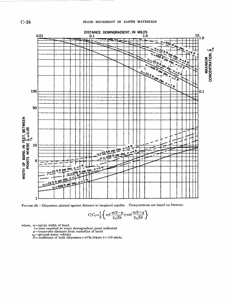
To provide some notion of the meaning of these data in terms of dilution and dispersion over long distances within an aquifer, the following idealized analogy is proposed. Assume an aquifer of finite thickness but of infinite area, whose physical characteristics are similar to those of the experimental medium; assume an injec tion well that penetrates the full thickness of the aqui fer; and assume that a solution containing tracer elements in concentration Co is injected into the well. As a function of the distance downgradient from the injection well, compute the width of the band of tracer elements between points where relative concentration C/Co=0.05, and compute the change in maximum concentration of the tracer elements, under the following conditions: (1) ground water velocity is 22.5 ft per day (equivalent to pore velocity of run llC), and ground- water velocity is 658 ft per day (equivalent to pore velocity of run 13A), and (2) initial width within the aquifer of injected band of tracer elements is 1 foot, initial width is 2 feet, and initial width is 4 feet. The coefficient of bulk dispersion D is calculated for each case from values of standard deviation obtained in runs 11C and 13A, according to the relationship D=<r2/2t.
The resulting computations are shown graphically on figure 28. It is seen, for example, that 10 miles down- gradient maximum concentration, which would occur along the centerline of the band, ranges from 44 percent of initial concentration for the faster velocity and 4-foot initial band width to 6.6 percent for the slower velocity and 1-foot initial width. The width of the band con taining tracer elements at relative concentration of 5 percent or higher, at 10 miles downgradient, ranges from 8.8 feet for the faster velocity and 1-foot initial width, to 22 feet for the slower velocity and 4-foot initial width. It is also seen that the change in max imum (centerline) concentration is sensitive to initial band width, and that the wider the band the longer the
distance of downstream travel before the maximum concentration begins to change.
In addition to the cases shown on figure 28, it may be calculated that where ground-water velocity is 658 feet per day, a band of 24 feet initial width would travel 10 miles before its centerline concentration would be affected; where ground-water velocity is 22.5 feet per day, a band of 42 feet initial width would travel 10 miles before its centerline concentration would be affected. In this connection it should be noted that in practical cases of fluid injection into permeable forma tions, the head on the injected fluid is apt to be con siderably higher than that of the ground water in the formation. Consequently, the initial width of band leaving an injection well is apt to be many times the diameter of the injection well.
COMPARISON BETWEEN THEORY AND EXPERIMENT
In a previous section (see equation 4c) the following was derived
For a given porous medium the denominator of the term on the rignt side is constant, and the term as a whole is dimensionless. This term may be used to transform the measured standard deviation of dis persion, a, into dimensionless form. Or,
r *_. (16a)
where <r* replaces yp f°r convenience in terminology. The length L is obtained by direct measurement of the porous block. The characteristic grain diameter d is, in general, not well defined, but for artificial media of nearly constant grain size it may be taken as the average grain size (fig. 14). A first approxima tion of the dimensionless constant a can be made by assuming values that seem intuitively reasonable. Referring to figures 4 and 5 and recalling that a=a^a2, one assumes that
that is,
that is,
aid (average distance between=0.5</; adjacent flow paths)
«i = 0.5;
a2d (average distance between=0.7c?; successive pore spaces along a flow path)
«2 =0.7.
C-24 FLUID MOVEMENT IN EARTH MATERIALS
0.01DISTANCE DOWNGRADIENT, IN
0.1MILES
1.0
FIGURE 28. Dispersion plotted against distance in imagined aquifer. Computations are based on formula:
where, w= initial width of band<=time required to reach downgradient point indicated y= transverse distance from centeriine of band
vp ̂ ground- water velocity D = coefficient of bulk dispersion =(r2f2t, /where t= 119 cm/t>/.

TRANSVERSE DISPERSION IN LIQUID FLOW THROUGH POROUS MEDIA C-25
Then,
By measurement Z,= 119 cm and d=.048 cm. These values are substituted in 16a.
=0.7<r.
In a previous section a relationship was developed
between <r* (=Vz>) and (o) H (see fig. 8 and equations
9b, lOc and 13), where
LetH*=(^}H (17a)
(I7b)
The last two columns of table 1 give the experimental values of <r and H, and <r* and H* are computed accord
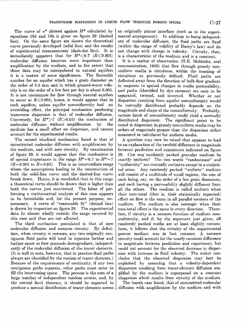
ing to equations 16b and 17b. It is now possible to make a comparison between theory and experiment. The theoretical curve previously derived (fig. 8) is re- plotted on figure 29, and on the same figure values for <r* experimental are plotted against H* experimental. The scale for Reynolds number is shown (see app., p. C-30). It is seen that the values of <r* experimental are roughly double those of <r* theoretical.
Perhaps most significant of the experimental results is the apparent functional relation between dispersion and fluid velocity. As H increases, dispersion tends to decrease. By the method of least squares, and the assumption that within the range of the measurements ff is a linear function of the logarithm of H, one computes that
a= 1.3-0.28 log ff/100.
If it is further assumed that, corresponding to each value of H, the measured values of a are normally distributed, the product moment correlation coefficient 7 is computed to be
7=-0.74
REYNOLDS NO. =
0.001 0.01 0.1 1.01.2
1.1
1.0
0.9
0.8
0.4
0.3
0.2
0.1
0
1
\
\\r*
\
^ MI
ur
d , b
\
19tri ffiVP
\
N
of jn isi or
^
n
"ire! on ou
^
iei fc d fi
«iStl
Vs
V
3T W ffca
l
jsonable fit' ricted molec nth amplific medium
*«.
^^^^^ *«^
\
\
etical curve unrestricted usion with n tion by pore
ular ation
v^
N, \
calcula molec
oampl us met
^
^x
ted- ular-bum
X
X,
0
c
'>
Sk
I
(
V
-
i*
i
s
x
-.
1
^Experimental curve of best fit
"^
.
^X
"-
^.
00o 8
^
^^,
ȣ <
^^^^
s
*̂""^
-4-^
c0
^^N.
»
-
'T
*N,
^
^ x fc
i
Note:
0
Points experir «=0.6 L = ll «/=0.(
calct nenti
9cm 48 ci
leoretical curve calculated for restricted molecular diffusion with amplificationb
,
y **
^
K
^
^
trousmediu
^^^
"* -
m
^"^
-
* ~^
jlated from al data for
m
». ^ ^ ^ ^
0.1 0.5 1.0 5 10
// /=/$/*//=0.09*}
50 100 500 1000
FIGURE 29. Graph of a* plotted against H*, theoretical and experimental.

C-26 FLUID MOVEMENT IN EARTH MATERIALS
and by Student's t test
£=5.9 (for 30 degrees of freedom).
The 7 and t values indicate that the probability of the correlation arising by chance is extremely small.
Converting a and H to a* and H* by equations 16b and 17b, the line of best fit is plotted on figure 29. It is seen that the slope of this line is approximately parallel to the theoretical line within the same range of H. This inverse relation between a and H supports the assumption that transverse dispersion is dependent on molecular diffusivity. The effect is measurable into the upper range of Darcy'flow. However, other mech anisms may operate along with diffusivity to produce dispersion; this is further discussed in the next section where an attempt is made to account for the difference in magnitude between <r* experimental and a* theoretical.
DISCUSSION
In the previous section a dimensionless measure of dispersion, calculated by analysis of an idealized model, was found to be roughly half that calculated by analysis of experimental data. It is possible to bring the two sets of numbers closer together by adjusting the dimensionless constant, a, and this would be proper if the assumptions underlying the theoretical develop ment were completely in accord with physical fact. However, as was stated in the beginning, the assump tions are simplifications and approximations. It does not seem fruitful, at this point, to try to refine the analysis by adjusting a dimensionless number, without being reasonably sure that this is where the error lies.
On the other hand, by making other assumptions and exploring other mechanisms, one might shed additional light on the significance of the experimental results. With this in mind, various possible idealized mecha nisms are listed as follows:
1. Unrestricted molecular diffusion of tracer elements with no amplification by the medium and with zero circuity.
2. Unrestricted molecular diffusion of tracer elements with amplification by the medium and with zero circuity.
3. Zero molecular diffusion of tracer elements and nonzero circuity.
4. Unrestricted molecular diffusion of tracer elements with amplification by the medium and with nonzero circuity.
5. Restricted molecular diffusion of tracer elements with amplification by the medium and with zero circuity (which is the theoretical model previously developed).
"Restricted" molecular diffusion refers to the ideal ization whereby tracer elements are considered to diffuse within a pore space, but cannot move out of it except by transport in the host fluid. The idealization is good for R > 0.04 for the porous block used in the experiments. It can be shown by use of equation 18a (below) that, when R > 0.04, the standard deviation of
the dispersion is less than 0.003 cm in the average time required for fluid to move through a pore 0.01 cm long. Hence, the bulk of tracer elements would be carried out of a pore space by fluid flow before they could move out by molecular diffusion. "Unrestricted" molecular dif fusion considers that tracer elements may move both within and out of pore spaces by molecular diffusion.
In the first idealization listed above, that of disper sion caused by unrestricted molecular diffusion with no amplification by the medium, diffusion would occur indpendently of fluid flow. Consider a porous medium (such as that used in the experients) half of which is occupied by fluid containing an initially uni form distribution of tracer elements flowing parallel to and in contact with fluid in the other half containing no tracer elements. Dispersion of tracer elements across the interface will occur as a function of time and of the coefficient of molecular diffusivity. It can be shown that in a semi-infinite region the standard deviation of the diffusion across the interface is
(18a)
In the case of a porous medium it is necessary to take the "lithology" into account, and
(18b)
The lithologic factor, /, accounts for the effect of the solid boundaries of the medium which inhibit the dif fusion of the tracer elements. For media of near- constant grain size its value is always close to 0.71 (R. P. Rhodes, oral communication, 1959). From table 1, Dm=0.64X10~5 cm2/sec, and L= length of porous block=119 cm. We substitute these values in equa tion 18b
and by equation 16b
<r*=0.7o-=2X10- 2 X
(18c)
(18d)
By equation 12c
where d=grain diameter=0.048 cm, and making the numerical substitutions,
H=7.5 X10V
By equation 176
(19a)
(19b)
TRANSVERSE DISPERSION IN LIQUID FLOW THROUGH POROUS MEDIA C-27
The curve of cr* plotted against H* calculated by equations 18d and 19b is given on figure 29 (dashed line). On the same figure are shown the theoretical curve previously developed (solid linej and the results of experimental measurements (dash-dot line). It is immediately apparent that for /7*<0.7 Off<0.005) molecular diffusion becomes more important than amplification by the medium, and to the extent that these data may be extrapolated to natural aquifers it is a matter of some significance. The Reynolds number for an aquifer which has a grain diameter on the order of 0.5 mm and in which ground-water velo city is on the order of a few feet per day is about 0.005. It is not uncommon for flow through natural aquifers to occur at R<0.005; hence, it would appear that in such aquifers, unless aquifer nonuniformity had an overriding effect, the principal mechanism producing transverse dispersion is that of molecular diffusion. Conversely, for /7*>7 (Jff>0.05) the mechanism of molecular diffusion without amplification by the medium has a small effect on dispersion, and cannot account for the experimental results.
The second idealized mechanism listed is that of unrestricted molecular diffusion with amplification by the medium, and with zero circuit}7 . By examination of figure 29, it would appear that this mechanism is of special importance in the range H*=0.7 to H*=7 (R 0.005 to 5=0.05). This is an intermediate range where the assumptions leading to the construction of both the solid-line curve and the dashed-line curve break down. Hence, it is concluded that in this range a theoretical curve should be drawn that is higher than both the curves just mentioned. The labor of per forming a mathematical analysis of this case appears to be formidable and, for the present purpose, un necessary. A curve of "reasonable fit" (dotted line) is drawn by inspection on figure 29. The experimental data lie almost wholly outside the range covered by this case and thus are not affected.
The third mechanism postulated is that of zero molecular diffusion and nonzero circuity. By defini tion, when circuity is nonzero, any two originally con tiguous fluid paths will tend to separate farther and farther apart as flow proceeds downgradient, independ ently of the molecular diffusion of the tracer elements. (It is well to note, however, that in practice fluid paths always are identified by the motion of tracer elements.) Because of the requirements of continuity, if any two contiguous paths separate, other paths must enter to fill the intervening space. The process is the sum of a large number of independent random events, and, by the central limit theorem, it should be expected to produce a normal distribution of tracer elements across
an originally planar interface (such as in the experi mental arrangement). In addition to being independ ent of molecular diffusion, the fluid paths are fixed (within the range of validity of Darcy's law) and do not change with change in velocity. Circuity, then, is a characteristic of the medium and is a constant.
It is a matter of observation (H.E. Skibitzke, oral communication, 1959) that flow through grossly non- uniform media is circuitous, within the meaning of circuitous as previously defined. Fluid paths are deflected away from the direction of bulk-flow gradient in response to spatial changes in media permeability, and paths (identified by dye streams) are seen to be separated, twisted, and inverted. Whether or not dispersion resulting from aquifer nonuniformity would be normally distributed probably depends on the magnitude and shape of the nonuniformity. Probably, certain kinds of nonuniformity could yield a normally distributed dispersion. The significant point to be noted is dispersion in grossly nonuniform media may be orders of magnitude greater than the dispersion either measured or calculated for uniform media.
A question may now be raised that appears to lead to an explanation of the twofold difference in magnitude between prediction and experiment indicated on figure 29. Can any randomly packed granular medium be exactly uniform? The two words "randomness" and "uniformity" are mutually exclusive except in a statisti cal sense. Any randomly packed "uniform" medium will consist of a multitude of small regions, the size of each being, say, on the order of a few grain diameters, and each having a permeability slightly different from all the others. The medium is called uniform when their sum-total (that is, their statistically expected) effect on flow is the same in all parallel sections of the medium. The medium is also isotropic when their sum-total effect is the same in every direction. There fore, if circuity is a nonzero function of medium non- uniformity, and if, by the argument just given, all randomly packed media are at least slightly nonuni form, it follows that the circuity of the experimental porous medium was in fact nonzero. A nonzero circuity could account for the nearly constant difference in magnitude between prediction and experiment, but could not account for the observed decrease in disper sion with increase in fluid velocity. The writer con cludes that the observed dispersion may best be explained by assuming that a velocity-dependent dispersion resulting from tracer-element diffusion am plified by the medium is superposed on a constant dispersion which results from circuity of the medium.
The fourth case listed, that of unrestricted molecular diffusion with amplification by the medium and with
C-28 FLUID MOVEMENT IN EARTH MATERIALS
nonzero circuity, includes all postulated mechanisms. For reasons already given, the effect of medium ampli fication becomes unimportant at very low values of the H number; at high values of the H number the effect of" molecular diffusion beyond individual pore spaces becomes unimportant. At intermediate values of this number the two mechanisms are of comparable magnitude. Medium circuity is assumed constant at all values up to the limit of validity of Darcy's law. The portions of the theoretical curves given on figure 29 appropriate to each of the various ranges, and for the particular medium studied, were previously in dicated. The effect of nonzero circuity may be included by increasing the magnitude of all theoretical curve values by some constant amount, say 0.5 hi this case.
The fifth case listed, that of restricted molecular diffusion with amplification by the medium and with zero circuity, is the model analytically developed in this report. It is not a comprehensive description of transverse dispersion, but it probably is the most complex combination of mechanisms that it is practical to treat analytically. The further development of analytical procedures probably will require the accumu lation of systematic experimental data; in particular,
data on the effects of increasing nonuniformity of the medium will be required.
REFERENCES
Crank, J., 1956, The mathematics of diffusion: London, OxfordUniv. Press, 347 p.
Feller, William, 1950, An introduction to probability theory andits application: New York, John Wiley & Sons, 419 p.
Kitagawa, K., 1934, Sur le dispersement et I'e'cart moyen del'6coulement des eaux souterraines: Kyoto (Japan) Imper.Univ., Coll. Science Mem., ser. A, v. 17, p. 37-42.
McBain, J. W., and Liu, T. H., 1931, Diffusion of electrolytes,non-electrolytes, and colloidal electrolytes: Am. Chem. Soc.Jour., v. 53, p. 59-74.
Miller, K. S., 1953, Partial differential equations in engineeringproblems: New York, Prentice-Hall, 254 p.
Pai, Shih-I, 1956, Viscous flow theory, I-Laminar flow: NewYork, Van Nostrand Co., 384 p.
Rifai, M. N. E., Kaufman, W. J., and Todd, D. K., 1956, Dis persion phenomena in laminar flow through porous media:California Univ., San. Eng. Research Lab., Prog. Kept. 2,157 p.
Scheidegger, A. E., 1958, Typical solutions of the differentialequations of statistical theories of flow through porous media:Am. Geophys. Union Trans., v. 39, no. 5, p. 929-932.
Taylor, Geoffrey, 1953, Dispersion of soluble matter in solventflowing slowly through a tube: Royal Soc. (London) Proc.A, v. 219, p. 186-203.

APPENDIX
Derivation of equation 9a of text:
n= 1,3,5 . . .
COS
n
exp-( (20a)
Integrating both sides of 20a with respect to y over interval w=0 to w=a
r c *,-&Jo 2 n
_ , ~~0 I
*
By equation 8
- «=1,3,5 .
exp \2o/
(20b)
(20c)
=-+- X O ' ^.2 ^-1
* TT n= 1,3,5.
Note: When t= oo, g=4
When f=0, 2=4+4 X)^ T « = 1,3,5, n2 22
Derivation of equation lOa oi text:The preceding solution for q(a,t) converges satisfac
torily for moderate and large t (low fluid velocity), but not for small t (high fluid velocity). It turns out that an equation that will converge satisfactorily for small t can be developed from the error-function solution of the original differential equation. This solution of the differential equation as given by Crank (1956, p. 15), letting h=a, and Z=*2a is
We desire g(a, t), where
(22)
The error function is itself an integral, and a method integrating it with respect to y over the distance a is not apparent. However, the integral is easily differenti ated with respect to y. We may take advantage of this fact by developing the following relationship:
Start with the differential equation for diffusion in one dimension
(23)
Integrating with respect to y over the distance a
/o^ N(24a)Intrgrating left side of above, and interchanging order of integration and differentiation of right side, we get
den 5 r« ^r\ H djMoJ
Because the fluid region is bounded at ?/=
hence,
(24b)
(24c)
Referring to 22 for any a constant, g is a function of time only. Hence, we may differentiate 22 with respect to time, substitute it in 24c, and get
dt=7T7 i-'a/ (25a)
We now integrate both sides with respect to time
(25b)
where A=constant of integration
when £=0, %=1=A
Thus,
q(a,t)=l- dt (25c)
C-29