A Transportation-Scheduiing System for Managing Silvicultural Projects

Jorge F. Wenzuela H. Hakan Balci

Timothy McDondd Auburn University

Alabama, ;USA

A silvicultural project encompasses tasks such as site- level planning, regeneration, harvest, and stand-tending treatments. An essential problem in managing silviculm projects is to eaciently schedule the operations while considering project task due dates and costs of moving scarce resources to specific job locations. Transporta- tion costs represent a significant portion of the total op- erating cost. The main difficulty in developing such a management system is finding an optimal transport sched- ule while handlmg complicated constraints, such as prec- edence and temporal relations among project tasks, project due dates, truck routing, weather, and other op- erational conditions. It is well known that finding an op- timal solution to these types of problems involves high computational complexity. They are usually NP-hard. For this reason, we propose to use simulated annealing -a meta-heuristic optimization method- that interacts with a network simulation model of the system in which the precedence and temporal relations among project tasks and logistics are explicitly accounted for. The approach has been tested using data provided by a silvicultural contractor located in Alabama. The results obtained solv- ing one instance of a small size problem with five worksites showed that the best solution could be found in less than four minutes using a personal computer with a processor Pentium Ill (1 GHz). A good solution for a larger problem with twenty worksites was found in thirty minutes. Also a resource analysis is performed to evalu- ate the impact of each resource on the best solution.

Keywords: Project management, silvicultural systems, firest operations, meta-heuristic, optimi- zation, simulation.

The &or are, respectively, Assistant Pmfmsol; and PHI Student in the Department of Industrial and Systems En- gineering, and Associate Professor, Department of Biosystem Engineering, Auburn Uiriversity.

INTR0I)umoN;

Silviculture is defined as managing forest vegetation by controlling stand establishment, growth, cornpsition, quality and structure for the full range of forest resource objectives [73. This is a broad definition encompassing a multitude of concepts, all of which must be translated into manipulations of a given trait or characteristics to effect some change at a stand or sub-stand. The range of manipulations used on any given stand can vary consid- erably, but as the science of silvicultuse matures the corn- plexity and number of entries into stands for manage- ment activities has tended to increase. At the same time, the need to reduce the cost of these activities has lead to specialized equipment and contractors to implement cus- tom prescriptions efficiently across many locations. When the primary resource being manipulated is timber, cost of silvicultural operations is of particular importance and new ways are being sought to reduce the mount of input resources needed to establish and maintain maxi- mum growth rate.

Forest landowners in the Southeast US, particularly large industrial forest product companies, often use silvicultural service providers as a means of implement- ing their management prescriptions. These providers can perform a broad spectrum of management activities at low cost, but, as in logging, there is always a need to further improve the efficiency of the operations. Service providers have turned to new technology in order to im- prove their cost effectiveness, in particular adapting tech- niques &om precision agriculture to reduce chemical ip- puts. Adopting logistical strategies use$ successfully in other industries also holds the promise of improving op- erational efficiency. Providing silvicultural services h i - cally implies perfwmhg numerous operations simultane- ously across a large geographic area. These operations share equipment resources. For example, a crawler tractor might be used for road improvement work as well as in site preparation plowing. Scheduling the use of these limited resources has a large impact on the efficiency of the entire operation. Equipment must be dispatched to sites in a sequence that minimizes total moving costs, primarily a fiutction of distance traveled, and that also accounts for temporal aspects of task completion. The scheduling process is M e r complicated by constraints on movement of the equipment and by external factors such as w e a k . Management and scheduling of these activities is currently done by people with experience in such matters, but as companies become larger and the number and complexity of jobs increases, silvicultural service providers are looking for improved methods of assigning resources to jobs in a manner that optimizes their operational efficiency.

Inientario~l ~ o m a i of Forest Engineering 4 67

the case that the resoutee unit has its own transportation (can move by itself), the w m p ~ o n is also valid. Figure 1 shows an example of a transport schedule (a solution) for a forest project with 5 worksites, two identical units of the resource class 1, and one unit of resource class 2. Here, worksite 0 (W,) is assumed to be a central worksite where e t m a n c e activities can be performed. The fig- ure shows that the first unit of resource class 2 is cur- rently at worksite 0 and is scheduled to visit worksite 4 and then worksite 3.

- - - - 1% unit of rescslrcr! class 1

------- lA unit of rcsaurce class 2

- @ unh of rcsowe dass 2

Figure 1. A solution for a multi-project problem.

Mathematical Model

We assume that the silvicultural multi-project consists of N spatially dispersed worksites. Each worksite is con- sidered one project. The quantity dq is the distance be- tween worksites i and j. At each worksite i (i4, . . .,N-I), a set of Mi tasks need to be performed. The set of tasks to be performed at worksite i is denoted by (t,,, t,. . -1. The task precedence relationships, resource requirements, and execution tirnes of the tasks are all part of a project de-

scription, which we denote by W=[ W *,.., ,.., WHY]. The due dates of the projects are denoted by D=[D,,..,D,,..,D, ,I. Figure 2 presents a hypothetical example of a project description outlining the tasks to be peperformd at worlcsite 1, project description W' . The figure shows the precedence relatioaships, duration, and resource rquireme~t of each activity. The available resource classes, quantities, and initial positions of each of the resource units are part of the transport description, which we denote by T = [T,, . . .,I;,:. .,TJ (R resource classes.)

The mathematical model for minimizing project durations can be written as follows:

Min z Subject to C = F(X; W,T); C 5 1 z; C s D

Where C is a vector in which entry i is the completion time of project i. F(.) is a Eunction that evaluates the com- pletion time of each project given the descriptions of the projects and transport, and the solution X. The vector 1 &notesavectorwith&eatries~to l,i.e. l=[1,1, ..., 11.

Solution Approach

The solution approach consists of two main compo- nents, a network simulation model and a search heuristic. The simulation model is used to evaluate the fuaction F, i.e. the completion time of the projects. The purpose of the search heuristic component is to select a good solu- tion X, and is implemented using a Simulated Annealipg (SA) algorithm. In the literature there are multiple applica- tions of SA to forest management and planning. 6hman and L W 1141 s;ndied long-term planning of harvest activities considering biodiversity, recreation and new road planning. They concluded that the spatial h e n - sion of the problem Fncreased complexity, but that the SA

* Fur example "A4 (8) r:f " meam that task 4 ofproject A has a dwat&n of8 hours and requires resource elms 3.

Figure 2. Description of worksitelgroject I;Y,*

66 * International JuunzaI ofForest Engineering The scope of scheduling silGcultural tasks lies within

what is called project scheduling under resource con- straints, which has been extensively studied [6]. One of the simplest project scherhrling approaches is the Critical Path Method (CPkf) 11 71. In this method, the set of tasks are represented as a network to denote the precedence relations among pairs of tasks. The god in the CPM ap- proach is to d e k d e the smallest possible project com- pletion time without violating the precedence relations of the tasks. The method assumes infinite availability of re- sources. A more realistic variant of the CPM is the Re- source-Constrained Project Scheduling problem fRCPSP) [lo]. Several approaches have been. proposed to solve the RCPSP. Pritsker et al. [15 ] proposed one of the first ~ ~ c a l formulatiom, a 0- 1 1- p r o m model to solve the RCPSP. The formulation requires the defini- tion of up to nTbinary variables, where n is the number of activities and Tis the number of time periods. The com- plexity of the model is O(n+mT), where m is the number of resources. More 0- 1 linear programming models can be found in [3,11]. Although the RCPSP is more realistic, it still has some limitations, One of the drawbacks of the RCPSP formulation is that it assumes constant availabili- ties of the resources during the planning horizon, but it is common in practice that machines are scheduleduled for znatn- tenance or they are required for other projects. Also, due dates cannot be considered within the RCPSP fbmework. The Generalized Resource-Constrained Project Schedd- ing Problem (GRCSP) [ 1 01 overcomes some of these linri- tations and has been successfidly used in manufacturing applications [4]. Despite its high practical relevance, the GRCSP is still not a good model for use in scheduliug silvicultural tasks since the method neglects transporta- tion costs. There is also a large literature on transporta- tion routing problems, whi~h are modeled and solved with various approaches 18, 121. The reader is referred to [Sf for an overview of vehicle routing problems. EIowever, these models do not implicitly account for the ordered sequence of tasks that may use these transportation re- sources.

This paper proposes a computer meta-heuristic model for scheduling simultaneously several silvicultural projects, each project consisting of an ordered sequence of tasks requiring the use of limited equipment resources. The rnodel implicitly considers due dates of each project, the order and nature of steps to complete tasks, task- duration times, resource rqeemen t constraints, task- precedence relationships, geographic location of the projects, transportation costs, atld due date violation costs. The goal of the model is to allocate shared e@en- sive assets and mhkike transportation costs and com- pletion time of the projects. The resulting optimization problem is a nontrivial geneialization of the GRCSP. To solve meaningful problems, we have developed an opti-

mization procedure consisting of a simulated m e a (SA) [ 1 6] algorithm that interacts with a network sim tion model of the silvidtwal md~-project system.

The paper has been organized as follows. In sectio we describe the proposed approach. In section 3, we scribe our experimental methodology and summarize rnerical and perf~mmce results. h section 4, a resot capacity sensitivity analysis is performed to evaluate impact of each resource on the best scheduling soluti

PROPOSED APPROACH

The problem of managing silvicultural projects can formulated as efficiently scheduling transportation 2

project tasks while cons ide~g project due dates i costs of moving resources to specific job locations. Sch ulkg transport among several competing locations 2

functions is critical in efficiently managing silvicultu projects. Transportation costs represent a signific; portion of the total operating cost. Trucks are needed delivering timber to mills and for carrying machinery 1 Ween worksites, which can be located anywhere withi large geographic area. A tramportation management s; tem that allocates limited truck resources optimally amo competing interests and takes into account project d dates cbuld increase the total operational eficiency o procurement entity.

Problem Description

A solution X to the transportation-scheduling proble consists of a set of routes for each of the resources th visit each project location such that all projects can 1 completed. A route specifies the sequence in which tl resource will visit the worksites. For example, for a set projects consisting of four worksites and three resow units, a solution could be given by the set of routes B ((1,4,3,2,3), (2,1,4), (4,2,1)). In this solution, resource is scheduled to start at worksite 1, then travel to worksi 4, and so on. In our formulation, we assume R differe classes of resources and that each class k (k l , . .JI) hi r, identical b i t s available. For example, four similar tra~ tors (three John Deere and one AUis Chhers ) may fon the "resource class" tractor. Each tractor is then a rc source unit. We assume that once an activity releases particular resource, the resource can st- its travel to ti next activity scheduled to use this resource unit. Tb rrext activity can be located at the same or at a remoi worksite. This assumption implies that if the resourc wit reipires a truck, the truck will be available to tmu port i t ~ot ice , however, that a truck can also be modele

a resource usit and it can be requested by activities. I

68 + I~tematiomZ Journal ofForest Engineering --

approach' could effectively generate optimal solutions. In another study [I], Baskent aad Jordan used the SA approach to solve a new landscape managemat model. They t q e d their model on a 20,q00 ha (987 stands) hy- pothetical .test problem. The result showed that the SA me&-heuristic technique was capable of solving large- size stochastic problems with hard c o ~ t s .

The SA d g o l i h starts by generating an initial solu- tion to the ttansportation-scheduling problern. Ln our ap- proach, the initial solution can be either provided by the user or generated randomly. The simulation model is next used to evaluate the quality of this initial solution. q e inputs to the simulation model are the data correspond- ing to the project descriptions and the tramport sched ule for the resources (a solution). The simulation model outputs p e f i o m c e measures, such as completion times for the tasks and distances traveled by the resources. The SA algorithm searches for a better solution using the infiormation provided by the simulation model and the current solution. We have implemented three neighbor operators to perturb the current solution. One operator generates a new solution by switching two worksites (ran- domly selected) of the merit solution within a route of a specific unit. The second operator generates a new solu- tion by switching two worlcsites between two different units of a same class. The units and the worksites are randomly selected. The third operator generates a new solution by moving one worksite from a unit to another unit of the same resource class. We use a random selec- tion process to choose the operator to be applied at each neighborhood-search. The search procedure uses the simu- lator every time that it needs to evaluate the pdormance of a new solution. An optimal or close to optiaaaX solution is obtained by iteratively rumhg this search procedure. Figure 3 shows a block diagram of the solution approach.

Simulated h e a l i n g [I 61 is one of the nature-hq heuristics that are applied to combinatorial optbiz problems. It was derived fiom statistical mechanics. algorithm, which was proposed by Kirkpatrick et al, is based on an analogy between ameahg treatmer SOW and solving cpmbinatofial opthimtion proble h - g is the physical process of heating a solid then cooling it down slowly until it crystallizes. At a gj temperatme, the probability distribution of system e gi& is determined by the Boltzmaan's probability ec tion:

where E is system energy, k is Boltzmann's constant, the temperature and P(E) is the probability h t the 5

tern. is in a state with energy E. To simulate the evoluf to thermal equilibrium of a solid far a fixed value of tt perature I; Metropolis et al. El31 proposed a Monte Ce method, which generates sequences of the states of solid.

In the d o g y between solving a combinatorial opti~ zation problem and the amealing.process, the states the solid represent the feasible solutions of the o p e tion problem. The energies of the states correspond to 1

values of the objective function computed for those so tioris. The miTlimum energy state conresponds to the ox ma1 solution of the problem and rapid quenching can viewed as local opthimtion. The basic steps of a SA goritbm are as follows:

Step 0: Create an initial solution. This is the first currc solution.

Figure 3.0phkaticin model.

Decide the initial temperature, number of repeti- tions at each teraperatue step, temperature re- duction d e and total number of iterations to be performed

Step Genmte anew set of solutiods h m the current solution.

Step 2: Evaluate the solution in tenns of the objective hction. Keep track of the best solution found so far,

Step 3. If the newly created solution is better, then up- date the cwlwt solution to the newly found better solution. If not, decide whether the new solution can still become the c e e n t solution, 4epending on Metropolis's criterion [ 137. If it passes the criterion, then the newly found solu- tion becomes the current solution; otherwise the m e a t solution stays the same.

Step 4: Iterate through steps 1, 2 and 3 for a defined number of times as decided by the n-ber of repetitions at each temperature step. After those many repetitions go to Step .5.

Step 5. Decrease the temperature using the decided re- duction criterion. Iterate through steps 1, 2, 3 and 4 for the decided number of times. M e r those many number of iterations, stop. Use the best solution found so far.

Using data &om a silviculture contractor located in South -Alabama, we have created a test-bed problem to verify our approach. The problem consists of four projects that are performed at four diffaent sites and one central site, namely worksite 0. Table 1 gives the distances be- tween each of the worksites.

0 107.5 2 3 330 82.5 1 - 1125 4375 1425 2 550 245 3 - 322.5 4 -

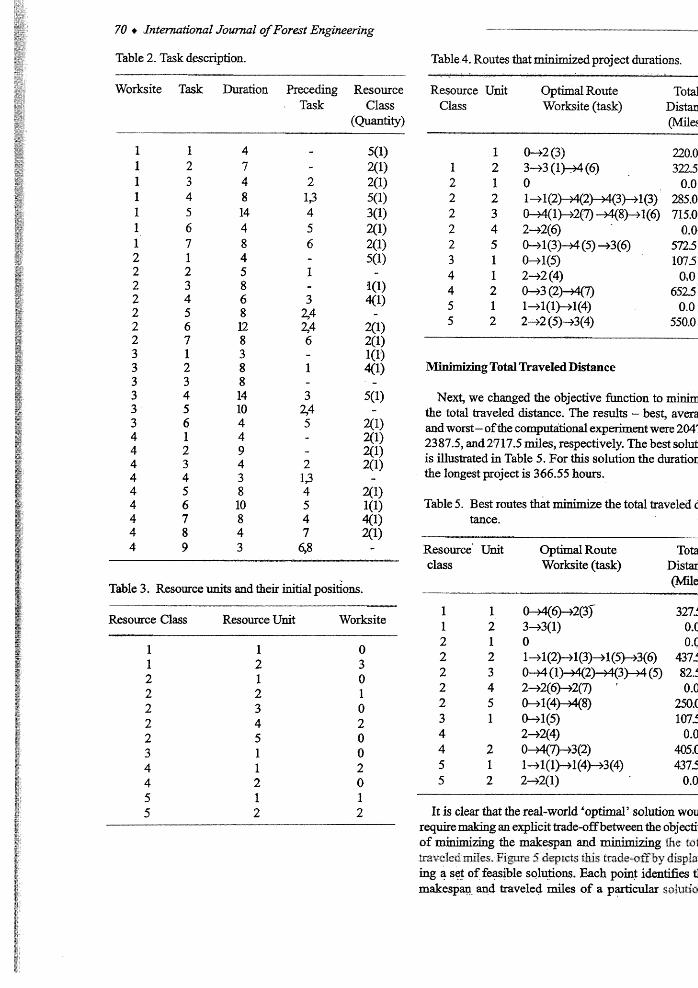
.Theset of tasks performed at each of the worksites are given in Table 2, This table dgcribes location (worksite), duration,.precedencet and classes of moveable resource

for each task.

We a s m e five classes of moveable resources are avail- able. These resources are considered critical for the op- eration of the projects. Table 3 gives the number of iden- tical xinits and their initial locations for each resource class. We assume that the resources move at a fixed aver- age speed of 50 mph. Notice that this assumption is not a restriction since each moving object in the simulation can be modeled to move at its om speed.

M' ' ' ' g Project 1)urations @&=pan)

In order to test our model, we first set the objective of the optimization model as rnhimihg the makespan of all the projects. The makespan of a project is defined as the completion time of the last task. Minimking project hations is equivalent to maxhkhg the utilization of the resources. After running the algorithm. several times with different parameters, we decided to set up the initid and cooling temperature of the SA algorithm to be 150 and 10 FO, respectively. In addition, the ternpera%e of the SA algorithm is decreased at each iteration by 2%. At each temperature step, the neighborhood of the currat solution is searched two hundred times. To evaluate the sensitivity of the SA algorithm to the initial~olution, we ran the algorithm ten times. For each m the initial solu- tion was randomly generated. The results of the test prob- lem -best, average, and worst - of ten replications were 225,23 1 and 253 horn, respectively.

To find whether the best solution was optimal, we com- putedthe objective function assuming an infinite number of resource units available. In this relaxed p r o b l q all projects can be independently completed at a minimum time, detemhed by the precedence relatiomhips only, and not by the availability of the resources. 'Ilie minimum makespan of this problem can be easily calculated by b d and it was equal to the minimum makespan of our best solution to the original problern. Therefore, we con- cluded that the best solution was optimaf. However, if they had not been equal, then, we could not conclude that the best solution was optimal. Nevertheless, the so- lution of the relaxed problem could be used, as a lower bound.

The best solution, for this particular case, which was also solution, the total distance traveled by the resowces was 3423 d e s . As shown in table 4, the 2"' unit of re- source class 1 had a route defined as ''303 ( I ) @ $ (@", meaning the initial location of this unit ~ v a s worksite 3 and it was scheduled to subsequently be used by the la task at the same worksite and by the 6& task at worksite 4. This pdcular route was 322.5 miles long.

70 + liztmational Journal ofForest E=ngrgr~e72'ng

Table 2- Task descxiptio~~

-= - -

Table 4. Routes that minimized project durations.

Worhite Task Duration I'meding Task

- 2

13 4 5 6 - 1 - 3

zi4 zj4 6 "

1

3 zj4 5

- 2 13 4 5 4 7 68

Resource Class

(Quantity)

-

Resource Unit Optimal Route Tog Class Worksite (task) Distar

m e

Table 3. Resource units and their initial positions.

Resource Class Resource Unit Worksite

M i n i W g Total Traveled Distance

Next, we changed the objective function to m i . the total traveled distance. The results - best, avm and worst- of the computational experiment were 204' 2387.5, and 21717.5 miles, respectively. The best solut is illustrated in Table 5. For this solution the dutatior the longest project is 366.55 hours.

Table 5. Best routes that minimize the total traveled (; tance.

Resource' Unit Optimal Route Tota class Worksite (task) DistaT

we

It is clear that the real-world 'optimat' solution WOL

require making an explicit trade-off between the o b j d of minimizing the makespan and minhhhg &e mi m.r.@led mila. Figure 5 dq1& this frade*Eby displa ing a set of feasible solutions. Each point identifies t makespan and traveled miles of a particular so8utia

Notice that the three points joined by the line dominate all other solutiom. All solutions lying on this line are called Pareto optimal solutions 121. Pareto optimality is a measure of eficiency. A solution is Pareto optimal if there is no other solution that makes every objective better off. A fhal decision that explicitly considers the trade-off between the makespan and the traveled miles should lie on or near this Pareto curve. Notice also that the raoge of the solutions is quite large. For example, there are many solutions that have the minimal makespaa of 225 hours, but have different total traveled miles ranging from 24 10 to 3400 miles. Eke, there is a potential for an improve- ment of 990 fewer miles. Furhxmme, without an opthi- zation procedure, the company could be operating at any point to the right of the line in the figure, for example the point marked 'A' where traveled total distance is 2750 miles and makespan is 325 hours. By using one of the solutio& lying on the curve, say traveled total distance equal to 2300 miles and makespan equal to 260 (point marked 'B' in the figure), the company could reduce the completion time by 65 hours (20%), and the total traveled distance by 450 miles (1 6%).

Iklhhbkg Project Durations and Total Traveled Rliles

The trade-off of makespan and total traveled d e s was modeled using a linear cost hct ion. We added a penalty cost of K, dollars per each hour that a project was over- due and a cost of K, dollars per each hour spent traveling between sites. We assumed equal o v d e penalty costs for all the projects for simplicity only. Introducing mer-

e t penalty costs for each of the projects can been in a ~ g h g o w a r d manner. The number of overdue for each project was calculated in hours as:

$3 Overdue hours = MAX (0, project completion hours - @

due date hours) (2)

In equation 2, the teJr "&e date" refm to the number of hours fiqm the current hour in which the project is requmd to be completed. The total overdue hours for all worksites was computed by adding up the individual over- due hours. Thus, the total cost of a particular schedule- solution was the sum of the total overdue p d t y costs and total travel time costs:

Total Cost = K, x Total O v d e Hours t K 2 x Total TnveI Time Hours (3)

In our example, we assumed that Y and I$ are 50$/hour and 80$/hour, respectively. Moreover, we assumed for this example that the due dates of each project were 225, 196,180, and 187 hours. After mmhg the solution algo- rithm, the best scheduling solution was fmdto have a total cost of $4,38 1. This schedule completed all the projects on time (before due date) and had a total traveled distance of 2,73 8 miles.

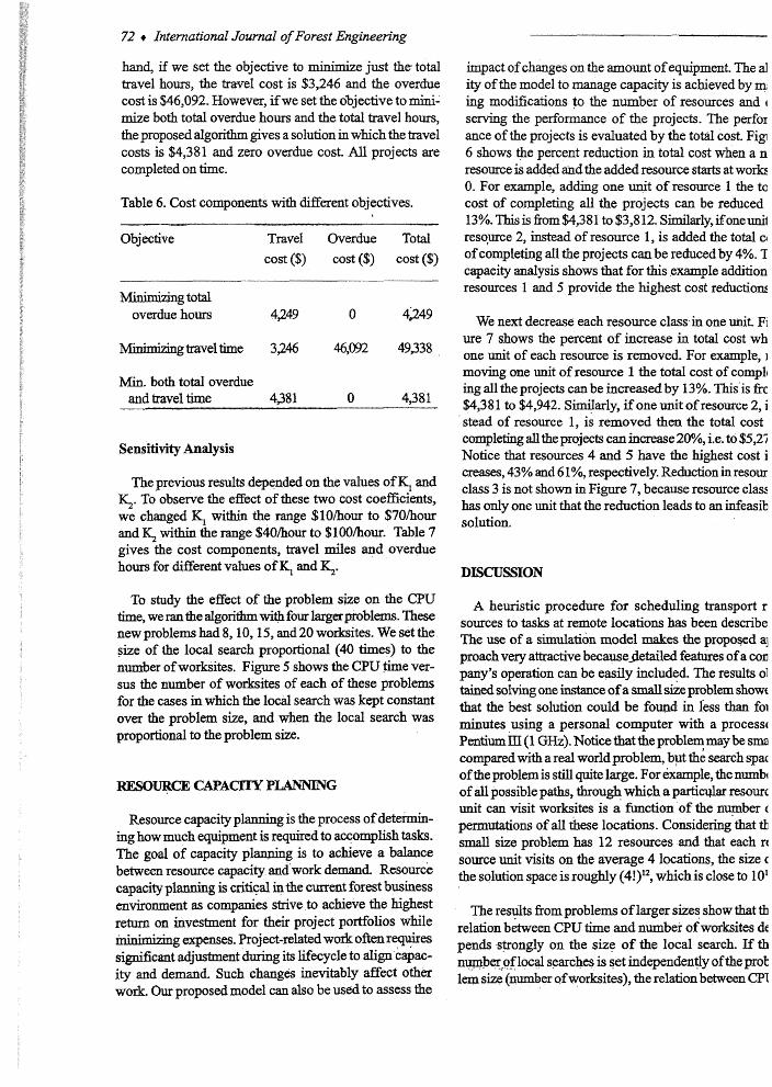
In Table 6, we have sunmarized the tot,@ costs by mini- mizing each cost component separately and && && simultaneouslyY If we set the objective to minimize the total overdue hours of the projects only, the overdue cost is zero, but the travel cost is $4,249. On the other

F i k e 5. Trade-off between makespan and traveledides.

72 + International Journal of Forest Engineering

hand, if we set the objective to minimize just the total travel how, the tawel cost is $3,246 and the overdue cost is $46,092. However, if we set the o%jective to mini- mize both total overdue hours and the total travel hours, the proposed a lgof ih gives a solution in which the travel costs is $4,381 and zero ovadue cost. All projects are completed on time.

Table 6. Cost components vvith dLfFkrat objectives.

Objective e l Overdue Totd cost ($) cost ($) cost ($)

MInimirsng@M overdue hours 4,349 0 4249

. . . . -gtraveltime 3,246 46,092 49,338

&. both total overdue and travel time 4,381 0 4,381

Sensitivity Analysis

The previous results depended on the values of K, and y. To observe the effect of these two cost coefficients, we changed K, within the range $lohour to $ 7 0 h and within the range $40/hour to $1 OO/hour. Table 7 gives the cost components, travel miles and overdue hours for different values of K, and q.

To study the effect of the problem size on the CPU time, we ran the algorithm with four larger problems. These new problems had 8,10,15, and 20 worksites. We set the size of the local search proportional (40 times) to the number of worksites. Figure 5 shows the CPU fhe ver- sus the number of worksites of each of these problems for the cases in which the local search was kept constant over the problem size, and when the local search was proportional to the problem size.

Resource capacity planning is the process of detamh- ing how much equipment is required to accomplish tasks. The goal of capacity planning is to achieve a balance between resource capacity and work demd. ~esourck capacity planning is critical in the ameat forest business envirollznent as companies strive to achieve the highest retuxn on investment for their project portfolios whiIe minimidng expenses. Project-related work often requires sigdcant adjustment during its lifecycle to align capac- ity and demand Such changes inevitably affect other w o k Our proposed model can also be used to assess the

impact of changes on the amount of equipment. The a1 ity of the model to manage capacity is achieved by rn ing modifications to the number of resources and 4

serving the performance of the projects. The perfox ance of the projects is evaluated by the total cost. Fig 6 shows the percent reduction in total cost when a n resource is added and the added resource starts at w o k 0. For example, adding one unit of resource 1 the tc cost of completing all the projects can be reduced 13%. This is from $4,381 to $3,8 12. Similarly, ifoneunil resource 2, instead of resource 1, is added the total o of completing all the projects can be reduced by 4%. 1 capacity analysis shows that for this example addition resources 1 and 5 provide the highest cost reductions

We next decrease each resource class in one unit. FI ure 7 shows the percent of increase In total cost wh one unit of each resource is removed. For example, I

moving one unit of resource 1 the total cost of cornplc k g all the projects can be increased by 13%. This is fkc $4,38 1 to $4,942. Similarly, if one unit of resource 2, i stead of resource 1, is removed then the totdl cost completing a l l the projects can increase 20%, i.e. to $5,2125 Notice that resources 4 and 5 have the highest cost i creases, 43% and 6 1 %, respectively. Reduction in resour class 3 is not shown in Figure 7, because resource elas has only one unit that the reduction leads to an infeasib solutim.

A heuristic procedure for scheduling transport r sources to tasks at remote locations has been describe The use of a simulation model nzakes the propowd a] proach very attractive becausehailed features of a con pany's operation can be easily included. The results 01 tained solving one instance of a s d size problem showf that the best solution could be found in less than foi minutes using a personal computer with a processc Pentium III (1 GHz). Notice tbat the probly may be sma compared with a real world problem, but the search spa of the problem is still quite large. For example, the numb of all possible paths, through which a paticqlar resourc unit can visit worksites is a function of the n-ber (

permutations of dl these locations. Considering that tk small size problem has 12 resources and that each n source unit visits on the average 4 locations, the size c: the solution space is roughly (4!)12, which is close to 10'

The re@& &om problems of larger sizes show that tb relation between CPU time and number of worksites de pends strongly on the size of the local search. If tb number$ local searches is set independently of the prol l a size (number of worksites), the relation between CP7:

Table 7. Total cost of best solution when travel and due-date casts are minimized

Kt % Totd Cost Overdue Cost Travel Cost Traveled ($hour) ($hour) ($1 (% of totaI cost) (% of total cost) nuJe

92% 84% 89?h Wh lW/o 1w/o 1wfo 1w/o 1w/o l w ? loo? 1Wh lWh loooh 1000%) lW! 1Wh loo! 1Wh 100% 1W? 100% 100% lW?

Figure 5. CPU time versus problem size (Pentiurn I l l 1 FHz and 256 MB)

74 + fitenrational Journal of Purest Brighering -

Add 1 to Add 1 to Add 1 to Add 1 to Add 1 to 1 resource resource resource resource resource dass 1 dass 2 class 3 class 4 class 5

Figure 6. Capacity analysis by increasing the number of resources.

Remove one unit Remove me unit Rmow me w&

Figure 7. Percent increase in total cost when one knit af a resource class is moved.

time and problem size is almost linear; however, when the number of local searches is set proportional to the number of worksites, the relation between CPU time and problem size becomes close to a quadratic fuaction- The CPU time depends more on the size of the local search than orzl the execution time of the simulator. Nevertheless, if a real world problem is too big tq be solved directly with our approach, the problem can be partitioned into smaller manageable sub-problems by identifling resources and geographic areas for each of them and using the pro- posed algorithm solve each sub-problem separately.

A silvicultural services company could achieve signifi- cant savings by using this approach to schedule its op- erations. It is well brim that transportation costs repre- sent a significant portion of the total operating cost of a forest products company. Additionally, transportation cost reduction has positive environmental effects as fuel use is miTlimized Future research plans are to incorporate into the shdation model random components such as breakdowns of maches or tmch and weather uncer- tainties.

This research was supported by the USDA Forest Ser ice Forest Operations Research Unit.

AUTHOR CONTACT

Professor Vdenzuela can be reached by d l at - jvalenz@eng.aubm. edu

El] Baskat, E.Z., and G.A Jordan. 2002. Forest lam scape management modeling using simulated ar nealing. Forest l!$cology and Management. 165(1-3 2945.

Caballero, R, T. Coma, M. Luque, F. Miguel, and1 Ruiz. 2002. Hierarchical generation of pareto optimi solutiops in largescale multiobjedive systems. J. c Computers & Operations Research. 29: 1537-1 558.

p] Demeulemeester, E., and W. Herroelen. 199'7. A bmch-md-hmd procedure for the generdlized re- somce-mnstrained project scheduling problem. Op- @ODS Re~ean:b 45: 201 -2 12.

[4] Demeulemeester, E., and W. Herroefen. 1996. Modeling setup times, process batches and ttans- fm batches using activity network logic. European J. of OperationaI Resmh. 89: 355-365.

[5] Desrosiers, J., Y. LhLIIliiS, MM. Solomon, and F. Soumis. 1995. Time constrained routing and sched- Ilfinp;. kM.0. Ball, TL. htfagmnti, C.L. Monma, and G.L. N&user, editors, Network Routing, Hand- books in Operations Research and Managaent Sci- ence, 8: 35-139.

[q Gordon, 3. and R. Tulip. 1997. Resource schedulhg. bt J. of Project Management. 15(6): 359-370.

Helms, J. 1998. The Dictionary of Forestry. Society of Amr ich Foresters, Bethesda, MD, USA.

181 Japsen, B., P.C.J. Swinkels, G.J.A. Teeuwen, B.A.. Wter, and H.A. Flewen. 2004. Opemtiond plan- ning of a, large-scale multi-modal trarsprtation sys- tem. European J. of Operational Research. 156: 41- 53.

[9] IhkpaQick, S., C.D. 3r. Gelatt, M.P. Vecchi. 1983. Op- thkation by simulated annealing. Science. 220: 67 1- 680.

- [lo] Hein, R. 1999. Scheduling of resouxce-com~ed

projects. Kluwer Academic Publishers, Boston, 392 P. .-

International Journal of firest Eneeering + 75

f 1 I] Kolisl?, R 1995. Project scheduling under resource c o n h t s : Efficient heuristics for several problem classes (production and logistics). Springer-Verlag, Heidelberg, 2 12 p.

[E'J Liu, ;ij.T., and C. Kao. 2004. Solving transporta- tion problems based on extension principle. Emo- pean J. of Operational Research. 153 : 66 1-674.

El31 Metropolis, N., A. Rosenbluth, M. RosenbIuth, A. Teller, and E. Teller. 1953. Ekpation of state calcula- tions by fast computing machines. J. of Chemical Physics. 21 : 1087- 1092.

[14] &mum, IL, T. Liixuils. 2003. Clustering of harvest activities in multi-objective long-term forest plan- ning. FOR& Ecology and Management. 176(1-3): 161- 171.

[la Pritsker, A., L. Watters, and P. Wolfe. 1969. Multiproject schedulmg with limited resources: A zerodne p r o ~ ~ g approach. Management Sci- ence. 16: 93-108.

[16J Vidal, RYV. 1993. Applied Simulated Annealing. Springer-Verlag, Berlin, 396 p.

[17'j WmStOn, W. 2004. Operations research: Applications and algorithms. Duxbury Press, Toronto, 141 8 p.

VOL. 16, NO. 1

Tell Us About Your Organization

Mitor's Note

P. Hakkila Fuel From Early ninnings

K. =hi& A. Jouhiaho, A. Muthinen, and S. Mattila Mechanized Energy Wood Harvesting Jir>m Early Thinnings

E.L. Lindholm and S. Berg Energy Use in Swedish Forestry in 1972 and 1997

D. Puttock, R. Spine%, and B.R Hhough Operational T'ak; of Cut-TeLength Harvesting of

................................ Poplar in a Mked Food Stand

IS. VEtEhen, A. hikaken, and J, Ekonen Improving the Logistics ofBiofie1 Reception at the Power Plant ofKt(opio City ............................................................

J.F. Valenzuela, H.H. Balci, and T. McDonald A Danqortation-Scheduling System for Managing SiZviculturaI Projects

J. Wmg, C.B. LeDoux, and L. W a g . Modeling and Yakdating the Grabbing Foxes of Hydraulic Log Grapples Used in Forest Operati~ns ...............................

VOL. 16 NO. 1 J M m Y 2005

A publication of the University of New BruRmicR