Transportation and Marketing Efficiency inthe California Processing Tomato Industry

Catherine A. Durham, Richard J. Sexton and Joo Ho Song

Department of Agricultural and Resource Economics

University of California, Davis

Giannini Foundation Research Report 343

March 1995

TRANSPORTATION M'D MARKETING EFFICIENCY IN THE CALIFORNIA PROCESSING

TOMATO INDUSTRY

The authors are:

Catherine A. Durham Assistant Professor of Agricultural Economics

Purdue University

Richard J. Sexton Profesoor of Agricultural Economics

(Jillvcrsity of California, Davis

Joo Ho Song 1-tirustry of Agriculture, Kwea

ACKNOWLEDGMENTS

Partial funding for !his ;Jt-Oject wes provided by the Giannini Foundatior •. The aut,_'mrs rue especially int'.ebled (:l

l.ee Garoyan for stimulntir.g our interest in L'lis project and tOr providing expert c.onsulta:ion chtoug,i.i:rut it<: evolution. We are <L.so gi:.iteful 10 the members ar;d cniployees of rhe Processing Torr.a:o Advisory Board foc ptQViding som.e ot!he data used :_'l th1s srudy, r.o Sam Logan, Rich Rost:nn:ly, a_<ill Jol:n Welty, who pro.,ided useful infonnatiou and advice, and w Songqm;n t,;u, who provided experr re$eMCh assistance.

SUMMARY

This s.tudy develvp'l and applies a no.1Enear mathematical programming model to detcmitne t.1.e Opti!flf.l al:ocat:ioo of ;woce$.Sing !O!lla!bt& :ro."fl the 13 largest produ..,ing oounties. i::i norlhem and central Califomia to the 32 processing facilities lo<:ated fn ~ area. The maL'iematica; m«.lel of :he indusicy Jit0cporatcs costs of h!Ouling iomatoes from field to procegsing fac1!it.ie>. and disting-Jishc'> between -i:lants Iha! process or:ly bulk paste and those tlw process diversified prodUIClS lncludir.g sauces, pllree, juke, and whole tomatoes The stu<fy· is also t~e f1rst ro inco:porate ex?IJ..iltly tomaioe!l' wluble solida oon:ent into the a."1.alysi&

A primary goal of the sn:dy is t0 evaluate the eftlclency of t.'ie allocation of tomatoe'l from farms to processing plants. Seven! foctohl have wntributed to long fICld-to·p!ant hauls in the California tomato indus-..ry. Urbanization h<ls shifted the pnm;icy location.s of production from the cenlTal coast to me cer.:ral valley. Several coasU: processing p1a.1ts now ii.IC-" a base uf localh:OO production. Ir, addition,

productlor.. peaks at different times in different producing r.egiom, so processors wishing to e:xtend their pw:::essh;g $Cil:SOn m1.1st incur long diMance h;iuls. 11'.e industry's uniftxm (M opposed to FOB) pricing ;;truCU!JI': also enccrJmges iong'"\'.lisum::e hauls,

ReS-'Jks of the analysis reveal modes! dcparrures froin efficiern:y in the prevailing tomato al!ura!.ior. pattern. The 11verage one·-way haul under the optimal all~tion was $6.7 miles vs. <16.6 n:ilcs for lhe !>$tirr~ actual a!Jocatron, with a resulting loss to lhe industry of $22 millioo « l.9% of g.--oss ptofit~ for 1989. Simul111ion of l'lnU)' of ix:w processing ptuns in Fresno and Yolo counties suggests I.hat new large-scale capacity pl!l?lts ln these locatitruJ WO'Jld be among !he mo;t profitable 1omruo pl'Oe.ts.sing plants in rtorthem and c.>-1tral Ca!lfomia. In general, the gimu1ation results reveal an industry where ?roceM'Or~· and produe>::rs' fates are closely l1md !Jlrough lrtU:rregional competition despite thetr being separated in many= by Jong di~ces and high traDsp«W'.an co~t~,

TABLE OF CONTENTS

I. INTRODUCTION ........... .

2. THE CALIFORNIA PROCESSING TOMATO MARKET 2 2.1. Consumption and Trade ..... . 2 2.2. Farm Supply .................. . 3 2.3. The Tomato Processing Technology .. 7 2.4. Marketing Arrangements ...... . 8

3. PR1CING AND TRANSPORTATION m A SPATIAL MARKET . . . . . . . 11 3.1. Spatial Pricing . . . . . . . . . . . . . . . . . . . . . . . . . . . . . . . . . . . . . . . . . . . 11 3.2. Spatial Pricing and Transport11tion Costs . . . . . . . . . . . . . . . . . . . . . . . . . . 13

4. THE OPTIMIZATION MODEL 14 4.1. Raw Product Prcxluctiou.......... . ...... . 14 4.2. Processing Plants ..................... . . . . . . . . . . . . . . . . . . . . . . . . . . 15 4.3. Transportation and Processing Costs ..... . 18 4.4. Processed Products Output ..... . 23 4.5. The Mathematical Mcxlcl ........... . 23

5. THE BASE MODEL SOLUTION: OPTIMAL VS. ACTIJAL ALLOCATIONS 27 S.I. Overview of Model Solutions .................. . 27 S.2. Optimal vs. Actual Allocations from Tomato Producing Counties in 1989 .......... . 28 S.3. The Estimated Value of Expanded Tomato Production ........................... . 33 S.4. Optimal Allocations to Processing Plants . . . . . . . . . . ........... . 36 S.S. Conclusions . . . . . . . . . . ....... . 43

6. EXTENSIONS: LONG-RUN EQUILIBRIUM AND NEW PLANT LOCATIONS . . . . . . . . . . . . . 4S 6.1. Long-Run Competitive F..quilibrium . . . . . . . . . . . . . . . . . . . . . . . . 4S 6.2. The bnpact of New Plant Entry in California Tomato Processing . . . . . . . . . 48

7. SUMMARY AND CONCLUSIONS ....... 54

ENDNOTES 56

REFERENCES 60

LIST OF FIGURES

Figure Z. I. Ci!ifornia's Ptoce.i:sing Tomato Produ;;tion and Value: 1960·'.992 3 F:gu.."'I! 2,2. Average ,\creage b)' C.:::rJnty 1944.-1946 . , , . , , . . • . , .. , , . . ... , . , 6 F'tgure 2.3. A'<wsge llcreag~ by County 19&1.1989 ....•. , , , ......... , 6 Figure 2"4. Seascnal Variation m California Processing Tooum PrOOuctil'.lr, uy Region fOI' 19&9 1 Figure 2.5. California Tomato Processing l'ltmt l..ocation~ ................. . 9 Figure 3.!. Marker Boor.daries iJrtder FOB Pricing .............•....... 11 Figu:n: 3.2. Market Bour.darie~ Under FOB and Unifmm Pricing • . .....•.. 13 Fig;;re 4. l . Production .w.d Plant Location . . . • . . . ... , . . ... , • , ........ . - ..... 14 Figt;.re 4.2. Processir1g RegioitS, _ . . . . . . . . . , . , , ..•. FiguN 4.3. Divcr.1ificd Plant Average Lal.xtt C~t Curve ........ . 22" Figure 4.4. Aver!ge Labor Com: Curves for Paste Plants . . . . . . . . . . . . . . . . . . . . .... . 23 Figure 5.1 Roads Linkirtg Region 2 and '.'\ Processors and Production ............ . Figure 6.1. Hypo1hctlcal Pl!lllt !Acar'.ons . . . . . . . . . . . . . . . . . . . . , . , , . , . , . " 49

LIST OF TABLES

Table 2.1. Table 4.1. Table 4.2. Table 4.3. Table 4.4. Table 4.5. Table 4.6. Table 4.7. Table 4.8. Table 4.9. Table 5.1. Table 5.2.

Table 5.3. Table 5.4.

Table 5.5. Table 5.6. Table 5.7.

Table 5.8. Table 5.9.

Table 5.10.

Table 6.1. Table 6.2. Table 6.3.

Table 6.4. Table 6.5.

U.S. Imports and Exports of Tomato Products: 1970-1991 Available U:iw Solids U:iads ....•........ Available High Soluble Solids. . . ................... . l 989 Plants and Estimated Weekly Capacities . . .... . Tr!!Jlsportation Mileage from Producing Regions to Processing Plant~ 1989/1983 Cost Ratios for Diversified-Products Plants ...................... . Nonlabor Input Costs per Raw Ton: Diversified-Products Plants ............ 21 Nonlabor Input Coses per Raw Ton: Paste Plants . . . . . . . . . . . . . . . . 22 Labor in Small, Medium, and Large Paste Planes . . . . . . . . . . . . . . . . . 24 Processed Product Production for Diversified-Products Plants . . . . . . . . . . . . . . . . . . . . 25 Aggregate Revenues and Costs for Tomato Allocation Models ..... . 27 Tomato Shipments from Producing Counties to Processing Regions by Season: Optimal vs.Actual Allocations .........•....... , . . . . . . . . . . . . . . . . . . . . . . . 29 Average One-Way Haul for Processing Tomatoes: Actual vs. Optimal Allocations ... 32 One-way Haul Mileages for California Tomato Producing Counties: Base Model Solution for Peak Production Weeks . . . . . . . . . . . . . . . . . . . . . . . . . . . . . . . . . . 33 Marginal Values ($ffon) of Expanding Low-Solids Tomato Production ................. 34 Marginal Values ($/Ton) of Expanding High-Solids Tomato Production . . . . . . . . . . . . 35 Operating Condition for Tomato Processing Plants Under the Optimal Allocation for the J989 Harvest . . . . . . . . . . . . . . . . . . . . . . . . . . . . . . . . . . . . . . . . . . 37 Excess Tomato Processing Capacity by Region: 1989 Harvest (000 Tons) ....... . 39 Marginal Values ($/Ton) of Tomato Processing Plant Capacity During Peak-Harvest Seasons for the 1989 Crop ........................ . 41 Average Shipment Mileages for Tomato Processing Plancs by Season: Optimal vs. Actual Allocation ......................................... . 42 Allocations and Mileages for Base vs. Long-Run Equilibrium Models . . . . . . . . . . . . . . . . . . 46 Allocations by Season for the Base vs. Long-Run Equilibrium Models Additional Marginal Values ($/Ton) of Low-Solids Tomatoes: U:ing-run Equilibrium vs. Base Model Solution . . . . . . . . . . . . . . . . . . . ....... . 47 1990 Processing Plant Allocations (000 Tons) for Base and New Plant Models 50 1990 Optimal Tomato Allocations from Producing Counties to Processing Regions: Base Model and New Plant Solutions ......................... . 52

4 16 17

. . . . . . . . 19 20 21

1. INTRODUCTION

!'mcr.ssing tomatoes are !..'l important end growing tigricuirural htdusey in California, but Ult industry is i."I a mm»dernblc stale of tlu:i: A$ we shall document in this study, the industry ls 1.<ndergoing rontin1.1ous change in !he geographic locations and sius of 1001aro· producing !'arms, In rum. these changes ate affecting die dynamic$ oI the proceSt>i!lg indu.'ltry. Processing firms localed in the highly u!OOnlzed San Fr~ncisoo Bey Area ccunties now ~lCk a significaru: base of loctdtzed production ro draw .ipon. These proce~s.ors must often source toruau.x:s from I 00 or more miles away. Meanwb:lc new pn1CCSs.!.ng facilities have boon located, mos; notably in Prosno County, in proximity to the largest crocentrations of mma10 production.

This gengrapbk evolution of ::he induscy is a do:ni.nant force affect'.ng competitive relations among processors and OOtwten pl'(ICCS'illl'li Md growers. in the short f!ln, nonalignment of producing areas /Ind processing locations has cr.used !omatoe~ to be hauled long dlsumces and haulage costs to represent 11. maj;ir expen~n to the induscy. JI has also stimulaled con~ide7a~ interregional competition among proce&<.ors w procure 10nuuoes. Over the longer ron !he industt)' is !C'lpouding to the geographic evolution of tomato production by gradually shifting plant location~. thr<rJgb the entry and ex.lt process. co beru:-r al@ piW'lt looations with the available production.

We esl'.rnate that !he avmge one·way hlwl for Cahfom!a processing to:natoeii n:rna\n;; in ex.ccss of 65 miles. Although this figure represents a long (tt,d ex.pens~ve haul, it i> a considerable redu¢lkm from the 100 mile haul estir.Jaw::f by Bnndt, Fre:x:h, and Je5se {1978) for 1973. Nmetheless, tlu: pereeption remains among indusli)· participants that tomatoos <L--e allocated inefficieruly acros> p:uooss.ing finm and ilia! reduced ltauluge and improved industry perforr.tance coc!d be attair.ed if a better grower-Mrprocessor allocation of tomatoes were 1.11::hie\•ed_

This study a.1alyzes the allocaUo.1 of processing tomawes in nonhem and central California and fL!lSCS5ei the efficiency of the prevailing alloo!ilion patt.em. We ~ a nonlinear optir.:lizatiou model to determ!r.e the optklal allocation of lornaioes from the 13 lru-ges1 proth:cing countiC$ in northern and ce11.tr1il California to the av-fillable pnx:essir.g facilities in this region. Wilh infor1:1ation olY,ained from !he California Proc-cssing Tomnto Advisory Board oo the actual allocation of tomatoos. we are ab.:e to compare the actual a!locauoa with Lhe e!ili:nared efficient ~location ruid e~tirnale

losses ti.I the Jndustty from inefficWm allocation of l«!lllWC& acrrn;s processing firms.

This srud~ represenis the first comprt:lieosive analysis of :he Califo,,_-nia tome.to industry slrux: the mid 1970s. Brandt, French, 11nd Jesse (197!!) and Brar.dt and Mench (197&) destribed 11.emand and supply conditions in the industry lhroogli 1976 and developed t11 econometric mode-I ot' 1r.e industry to evaluate t¢0'!lontic impacts of mechanical tomato r.a._-vest\r.g and dfvelop proje<:tif!rui fur indnstry growth fro1r. 1980-90. Chern &nd Just \1978), also dcvc:oped e<:onometr.:c models of L1e industt)' usi.1g both aggnogaie an..1n3\ tlme series dnta from 1951·19'75 for the 10 lugus1 pnxtucilig WJnties ~ by pooling ..:ounry·lt:vcl and time-S<'rics dal.!. This stud> also to evaluated the imp.act of :he tomato har.-esre1\ Among the conclusions was that observed ntl!'ket responsell to Ll-in hiinestcr were oonsiMent with ll1l oh_gopron~ market structure in procurement of raw tomatoes/

The antecedent t<> th£se orudies and the first comp."l':~mive an:Uysi;; of the California ptoceshlng tom;;to industry was analysis of g:rower~sor integration oond:.icted by Co:lin&. Mueller, and Bin:/-. (1959). Thi$ itudy providerl the firot in-depth analysis o: lhc growa·procewJn contract5 that prevail to thi;; day Jn the indm>try.

'Tht! present study il' disllnguished from its p:icdecessor5 in undenaking an oplimizatin.n ralher t.ha.'1 an economeuic franwwmk and focusing speci_fic;;Jly on Lhe rubjec:t of opllmal grower~:o-pro:esscr allocation of tomatoes nnd mmspormtion efficlenay. Chap!ef 2 provides an updarnd descrifXlon ef. the processing tomaio industt)', including oonsumptioo and trade, farm supply, processing. aud rr1arketing mangemeu&;. Chapter 3- develops some conceptua'. point$ :;;onceming pricing and uusponi;tion in a sp;:::ial markott. In p&r.icular, it is shown lhru. !he cniform pricing systcnt empluyed by the iudastry n. o:eruiin to lead 10 ineffic!eut tnrnsportation re!ati~ to an FOB pricing sysrem.

Chapter 4 i;et; forth the o;nimiz.ation model a.'1d describes dam s~ used to parallli'M:rlze Lhc model. Tite main anJ.l:ytica.I results are provided in chapter $, Where optimal vs, nctual tomato "11octititmil rue J_YreSented and compared. Chapter 6 e>:tends lhe model to lock at a long--rJn equilibrium fon:i.ullilioo and to si:nulaui the entry of new pt"OCessing plants. Finally. chapter 7 often. couc\uding commertts.

2. THE CALIFORNIA PROCESSING TOMATO MARKET

Toniatoes are the se.cond hig!11'.l't •alued ~-eget;1.ble crop Jn the U.S.. ranki:ig only behind pWtoes. Jn 1991 California produced 9.89 million tons of proces~ing !Dma:oes, 011er 90 percent of the tmel V.S crop. Processing wma\oe>. are Im inregml component of California's JWieulturel economy. ThJ 1991 crop generated $640.i million, making processing lntr.atoes the Siai.e's highest valued ¥t'lgetable crop arul eighth highest value atmculturn.l product overall

Producl.ion of processing tomatoes has iTh.--reased rapidly in Cal!fo."!lia in re.cent years as Figure 2. l documents. The 19!!? harvest of 8,6 million kl:'IS !lbatte~ the 1975 reoo:d harvest of 7.3 million loru. Production :ootinued kl rise until 1991. Produetioo was reduced to 7,9 millmn ton§ in I'm, ail a comequeiwc of the dechoo in finished prod:.ict ;irices. This chapter de5er.bl:s various dimensions of this important California in:lu~rry. including consumption aiid trade. farm FUpply, che _prooemng ~ootor, and marketing :md tnmsporuu.ion MTI!l'$'menrn.

Consumption and Trade

Processed tomato produa.!l form & major purt of U.S. ..-ege~ble iru.&ke, rank.ill.£: fmt among fruilll a.1d vegetahles in contribution.~ 10 the diet. Per capita coosumptloo of process«i :omaio products in 1;ie U.S. rose from about 62.! lbs. farm weight in 1970 to 70.J lb. in 1990, p-0.ftly as a result of the intreued demaml for Julian and Mexican food produC'ls.

The increase in value· added produc:s, such au I!alian sauces and Mcric1m foods, produced either fm h<.'.!':ru! une oc for !he food servloo indusuy, have alrered tl'.e composition vf production. Bulk p.ure is now ,;old comrr.cnly as an ingredient to <Mer food :nanufacturers. S:ime procesoors purchase twnatoes from growen and mamifacrure and s,ell processed good~ such as pastll produC'ls. Consumer preferenC'es in bnlllkfasr beverages have brought about a decwaSI.' Jn tO!llato Juice production as conrumers have shifted to oran~ juice.

Fa;;ton; influcn<:irtg the demand for tumatoe~ include rising coosumer incomes, ,,.,.·hich generally diminish the derumi for cannc<l vegetables whi'.e increasing the i!errumd for fresh produce. Demand for C<Jnvenlence foods and food servi~ bas \ncrea:ied as house!wld composition has changed. Tom.lt<ies form an imporUL.1t '.11greclie111 in the fast food ar.d res:autant industries.

Wo:Jd dernand for tom.am products is ilio rising. allhough per capita consumption rates differ widely acn:l;l~ u>:.n1tries. For l9SB·9!J the U.S. "'itt ~ large$t

per capita coruiun1er followed by Italy, Grtt:ce, and Canada. CQUJ!tries that pre;;en!ly :;:onsume little pm::es~ed tomato pro;iucls include Japan and ihe UK (8.S ood 18.5 lbs. farm weight per capita, respe.:tivety),

·rable 2.1 !.llmmarizes U.S. import wid export volun"".es for processed too<.ato products for 1970-91. The U.S. has ttaditiorally been a net importtt of both tomato paste i"\l'ld sauce. However, the US. export volume of these :;:ommodlti.es began to increase rapidly :n 1939 zoinciding with the series of reco:d California harvests. In t99l The U.S. wa.11 a net exporter Qf past11 for the first 11tne. Sauce has also IDO"<ed s!Iongly lnto !he. net export caregory after having been a net impon prior 10 19&8.

Sullivan (1992) cites sttor.g demi"\l'ld fQf klmato produ.;ts among newly iodumialiied countries in Latin Amerlcii, !he Caribbean, and Asia. U.S. e:icpons, hmoiever. ha'>'e continued to wge1 traditional markers in Canw.:lil and Jap!t!!, leaving CbUe lo serve the emerging mad::eis. J>aste exporu to CMada in 1991 t0rolled 61.1 million lbs., 64% of total ll.S. paste expqns. Japan was the woond largest paste 1mpurter with 16.4 million lbs. Canada also a:;:coun!OO for 64% of U.S. tomato sauce imporrs"~50.5 million lbs. while Japan imported 9.3 ntilliw lbs. during 1991 .

The t:.S. has traditiO!!ally impMed &.e greaie;;t amou:it of tomli.ln ;iroducts frQ!T. the European Community. In. 19U8$, 51.3% of U.S. tomaro pl!!li&

imports were fuxn the F.C. brae! was: secon\i in puic imJXlrts at 17,3%. with Mexiro tJ:ird at 13.0%. The impoo: :tltumion has sltfted dramatic.ally in the past several yean.. bo'>W;ver, d!ie to esLilblishmer.: of prOOuctioo quotas on srrbsidiied F..urope:m Corruuunity prOOuction and impru:itlon of higher wiffs (from 13.6 w 100% of valV() on l!npons from U-.e F.C k> ~

United States beginning in 1988 ln retaliation fo:: !he EC"s ban or. honnone-fed meat produci:s. As a resutt paste imports from the EC hive t11senciaUy disappeared and Mexi¢1 is nov. the domin!tTit exporter c-f pa!!lt: to the U.S., shipping 59.'.l million lb~. in 1991.

Mexico's pn;ic;es\ing: tomato lndusuy is CQf!CCntraicd tn &.e Si:ialoa region, where 8 of 10 Mexican pr0001sing firms are ll'.>Cated. The current industry p!'OO{!'>sing capacity in Mexico is soo.ooo metric tuns pe:- year (U.S. DeplUtlllent of Agriculrure 1992). Imest:Jr.ent ia pro«Siing ca:paciry in Mexico i> expected ro ir.crease partly due IO new Mexk:an laws that will faC:lit.ate lnv(:Sunent by U.S. firms.

Mcxk:rut yields are only half an high as in CaJifum\a. This factor coupled with high shipping eOJl3 Md a t.11.riff of !3.6 pe-r<:ent have to date off.;;et

'

Figure 2.1. Cal1furllla's Procewlng Tometo Production and Value: 1960·1991

lO '

" c D L

8'

8

;,._?DC

60'.1

0 0 0

L 0 0 0

50C w

.;oo

;300

' ~2'.J{l

c ~

c c-' ~

;,, l)C

c

[ --- Tons ---+--- lJaiue

Mexico's comparativeiy lower proce~ing eQSts. However, tariffs rue S\:heduled to be phased out under the N<irth American Free Trade Agreement (NAFrA}. auguring a sign.ificim; increase in ~lice's OO!Ilpetitiveness for U.S. proce1sing tomato sales.

The final ouWOmt: of the GATI negoti111ioos may ha'<e tittle eff«;t on F.uropean e~poru to the t:.S., since new foreign pmducen; have l.:egun sh.ippm.g: to !he U.S. msrket 111 low COSL F-Ot aample. Chlie has emerged as ;; furre on I.he i:ntema!.lonal tomfilo products market wnh a 24.2% share of U.S. past¢ impo~ Israel is now third at f.L2%. Tomato production is also ew,crglng m a number of other locations including ~:em Europ:: {Bulgaria, Hungary, and Yugosla"ia), Asia (lndla and Taiwan) wnJ South Amer'&& (Argentina and Brai.il). Many of theSt nations have t.ie wil and climatlc coodltions necess&ry for lt!Crna:iingproduclion. However, infra~tru::tnrc to support efficient and competitive production appea..-s 10 be a major factor Umiting expansicn of prodt..clion in some cases. In addition, high U.S. pr(J(fuction levels in the l~ have reduced world paste prices 1111d, thus, irn"'.entives to ~pand producti.:m.

2.2 Farm Supply

As of J993 there were 486 growe!'11 ti prooessing l0Jnalne$ in Ci!ifo:ni11, The average grower plants around 500 acres of torr.ai:oes annually. The historic peak in harvesred ~ge for Ca:ifomia p:ocestililg iomaroes was ID 1975 at nearly 300,()(X'.I, In }>llrs

between 1975 and 19&9. h!UVeSl'!ld acreage remained below 250,tro acres wtlh lhe exception of a barvttt of 276,()(X'.I acmr in im.. llowever, acreage began w boom in 1989 with 276~'!00 acre1 and then Increased 10 a new recon:I high of Jl2,0CQ acres in 1991, Low prires inspimd by t.hroo SUCCC\Sl'itl large C!"Oj:>5 prompted a slurp ~lQl"l tn coor.racred acreage w only 240,00J ~in 1997.

Yields bave alroincreased. From 1986-91 yield °'"'"'.ts

m.:ite in !he 29.32 tons per acre ra,...,ge. By comparison yield in I.be 1970s range<: from 22~25 LOI\$ per acre, Signific.'.l..,t improe;emen1s in yield 11nd sdlids oonlen1 have come with new tor:iato varieties anct imprl'."l..-ed pest and weed ooi::.rnt

Most toniai:a gn;iwers produce crops in addition to tomatoes. Rollltion with other crops mainr.ain~ productivity of individual fields, Wheac and sugar

3

T•ble 1.l. U.S. Imports ud Exports of T11mto Prodoct.s: 1970.1991

y,., Tomato Imports (000 lbs.)

Paste' Sauceb Wbol• Pllip ·~~

Tomato F..lporu (O!X> lbs.)

Sau:e Juice Catsup Olhet' & &

""= C!tlll

1970 91,382 128.534 9,994 4,501 l3,4Tl 6,967 19,146

19'11 "'~"' 108.557 6.1301 3,467 12,345 7,109 17,3&1

1912 126,241 l58-,6JO 8,161 7,246 11,452 7,534 19,!/23

1973 118,915 JOt,146 36,922 6,552 21,429 9,941 24,699'

1974 4S.218 66,051 4&.333 6,419 20,263 \0,838 26,651

197l 26,881 68,914 22,176 6,142 32,828 15,014 30,143

1976 5:5,237 74,160 24,Q!2 8,8!6 46,982 15,&64 23,621

"'" 65,198 12.m 28,591 6,117 41,684 14.714 2£,295

197• l0,991 7,116 74,t65 4.217 26.649 5,739 3-0,1161 18,303 28,195

lm 41,0Sl 2,794 45,567 2,881 38,333 7,395 25,060 l&,078 41,685

'"" 2S,"6 l.651 39,S&l 3,673 Z!i,404 6.421 32,512 23,852 34.952

""' 6',1fil 9,116 97,23(). 2,088 24,554 9,014 34,963 27,754 32,194

1982 198,029 21,824 167,018 1,301 22,556 6,315 29,284 27 ,58{) 19,987

1983 160,742 23,6U 186,709 875 23.964 6,701 18,552 23,455 14,002

1984 151,(145 """' 213,567 76: 21,203 5,895 :4,032 20,362 :1,953

19'l 111,400 33.588 220.028 l,398 15,691 4.723 l I,9&4 l8,082 15,919

19'6 130.625 197,559 197.559 Sil 17.234 6,187 15.000 18,902 13.902

1987 101,247 178,Sa'! t711,587 2,5{)6 20,440 M19 13,272 23,450 8,040 ,... 107,655 175,528 175,528 4,752 26,{;18 18,662 ~S,869 Z6,447 : 1,842

19S9 228,400 lll,590 tll,590 1 i,233 30,302 58,781 12,818 25,782 9,124

1990 136,1113 137,292 !37,292 6,988 84,724 53,8113 16.524 35,197 14,189

1'91 94,954 114,840 114,840 S,700 97,257 79,145 6,300 35,200 17.600

• tn.:lud.1$ '*1ice prim Ill !97R t T~~ rontm:ling N1artitmt.l ~nillg& not iru:ludrd prior w 19&9. • Produebi oot cla.uifie4 Jbfw~

S~ Yttitfilhktmui Sprcio.ltlt.<: Slrna!ia11 and Ourlook Y~ariJook. 1J.S. Dep$:1ment of Apiculnne, &ooorn!c Research SetYice, Dix. 1991.

•

beets aft! cQmmonly rotall".d with tomatoes. However, the specifl\: crop used in rotation varies by area of the st.ate. Depending upon the market and local producing conditions, the Sll-'11e !ield may be planted in lomatocs for COns<X;>itiYe years.

Historically 1001ato production was quite -...idespreOO in califomia as shown i;; F'igure 2.2. which de'pkts tomato acreage in the mid 1940s. The darkest-shaded counties repreiµ:nt the greatest numb« of ocres. During the 1940s over 3DOO growen pnidnced on a11erage 32 acres of tom.atoos fo: either the fresh or processing marke~s.. The iocatico of production hM cl:=ged ronsidentbl} since that time as c.omp;lrison of Flgure 2.2 with Figure 2.3, whiclt deplcl.!I acreage level~ in Ute late 1980s, il\uscraoos. Urban expansion brui been lhe pr'.mary factor in eliminating prowssing tomato acceage ln ~ Angeles, San M<.1eo, San Diego, and Alameda Co:.inties and reduo;.xl it more than $!)% in COUl'\!ius such as Sacramento and Santa C!Ma. Fresno County is now the top productt' in 111¢ state after having no am:s reported in 1900. The rise of prOOuction in arid counties such as Fresno is p;;imruily a rewlt of extended irrigation and drainage projecb;,

Along the California·Af.rona border Jn the [mperia< Valley, it is possible to harvest t¢tnatoes almu~t 1X1ntinul'l.!ly fTI;im mid-May f(I mi<l-Novembcr, althoogb in recent years harvests have ended by July. In genera! the harvest sna$on lasts 19 weeks wilh lhe major pan of productioo occuning be(wcen July and Septembe-r (Monl!on anC Pracl!am 1988.;.

Clir:u1~ pattern!> acrually al!ow harvest 10 begin ir. lhe Nortl;em ::nost producing county, Cclusa, nearly as early a~ Jn Fresno County, ow:r 150 miles to the south. Coasml counties such mi Monterey, San Denlto, and S:mlJi. Clara begin pll)duction sewxal weeks later. Late production io all are.u is vulnc:able to wC<tlher problems. Occasionilly uns<:aronab!e :rains affect peak ha.-wzst periods as well. 1n 1976, far example, nearly 34,000 acres were Jost as a result of rain iu Augu$t and Septernber. FigoJn: 2.4 depicts Ute weekly harvest pattern for the various lOl'rulto pro<lueing regions in Califurn.ia.

Average time from emerg~ to b3tVelit is 125 days, but emerge~ and tht peroonmge of marure (ripe but oot overly npe) frtlit at Mtvcst are strongly effected by planting date, Sims et al. {1979) foond that tnmatoe$ p!ar;!ed on Match 4 took 25 days ~ \IIT!erge for a July 31 h,orvest dare wlth 85% rnarurity.1 Peak m.at'Jrlty cf 93% occ1L~ 'l'-itb a May 12 plaru.ir.g dale, 9 day emergence, md batve$t en Septen1ber 23.

Sinoe the adoption of the mechanical harvester in the 1960s, there have bun only minor chrmges in

production r.ecb.nolugy. 1'he harvester has enabled larger·srale farming and contributed to alleviating the labor shortages creal.t:d by the end of the Bracero

1program • LaOOr requirements changed from fltlld laborers 10 ~rter tahoren;, who sit uport the ha:tvestnr ar.d rcm-0ve wn·scaldcd, wormy, ar.d moldy fruit as it p&gses by diem oo a conveyor belt. Electronic Y.l'l1er$ umove ~n frull and dltt (Sims et al. 1979).

Proccsslng tomatoos are grown with speelfic chnracteris.tics for diferent end uses, T001&1oos with a high oolids cootrnt produ"" more outp1.1! of prodl.lrts which are defined by ~ir soJid~ 0001.enc incluCing paste, cats\Jp, and sauces. Some varieties provide greater flow consisw.ncy which is important in son1e ptoduca including (13!$Up and spaghetti sauces. These varieties can be- b:ended with high ~olids varieties to provide the proper mix. Varieties wich ur.lformiiy in size 1L°1d color are< especially imporunt for \oOho:e llJl<! diced produet>\

Califnmia tomatoes a..'C inspected prior to delivery at inspection stations 011erseeu by the J'>rotewng Tomato Advisory Board, a joint boa:d Qf growm and prccesW!$. Two samples furn each load CT tomaioos a.re inspected fur defects such !iS sun $0.!.kling. under· N over-ripeness, motd, wcrm~, m.a!erial other lhlll'l torttatoos. ttc,. and te.~ted for soluble ~olids content and coloL E:w;cesses in die defect category permit rejection. buc typirally defects are at a low level, and payment is simply reduced by the percentage of dtfocts over an allowable pnrccnLage (0 (o 5% depcnd!ng on type of defect). Tt-.ese penalties provide iru:u.iives for the growcr to maintain reasonable stmd&rt'I$ at the fieki sotrlng iewt Soluble solids con"tent premiums are paid by many p~. Thebe prtmiiuns provide in~tives fur c..1-0osL'"lg hig::t-solids cooter.t w:uato varieties and discourage lalf .applications of water which wou:d raise the welght or yXlld pe; a~ v.ithout providL'"lg co:::nrncnsuralil additional solid~,

Information on the characteristics of a load can be u!!ed by multiplant processon to determine the best processing site fur it. A lost with high s.oluble solids roay for insrnr.ce be. delivered ta a plant primarily or wl:xilly devOl:ed tn paste mant:.facnire. Alierna!lvely, at die plant level the information may be u&etl HJ help deu:nuine wrJeh prod'1Ct line the iacortti-ag lna.d cf tome.lots will be sent to. mplants that process diYCnle producm~whole tomatoes.. $fillCCS.. v.uu, ;>asie, etc.· the romaroes with a better appearalR'e aft! u:>wtlly diverted to whole tomato lines, while t.omru:oes with high solids ctmient nre preferred for use in pastt: and sauce products.

'

6

Figure 2.4 Seaoonal Variation in Callfornl.a Processing Tomato Prod1N:Hon by Reglun for 1989

30~------

,, 1

~ ,,]

r=•="coASTAL -+-- NORTHl::: S. CENTRAL -- TOTAL

2:.3, TM Tomato ~sing Tecb.ootogy

In 1989 24 to:naro prod!Nt canning !UXI paste firm~ opemtt(I 37 plantll for {'f<Xl(!$$lng tQrnUWl:s in Califurnia, ;u compared «.; 57 fllTl.W ope-rating Jn l955, Since 1989 five plants have opened and slx plans have closed- lo OOdition. them are a few firms which use only a few IMS of «.truatoes annually. inc!uding fruit !UXI vejt!tab1e ~ft and ~s and • liquor :rttanuf11o>:lufM

Figure 2.5 depic'"Jl the ltx:atimi and various sizes of plants in Ciltlfurnia. All. X, I., M, and S in the ligtre ~~ 1 plant processing OYCt" 500,000 rnw tons &ru1ualty, from :;ro,ooo to soo.oco ton~. from 210,000 to 350,00J tons. w1d from 60,000 to 200,0ClO rons. respectively.

The lstgest single prooes.wd prodvr;:t by volume of inpl.lt. a& well as finished product, is tomato paste. This cate&ory includes bulk production to be oold to other food manufacrurers. Over 10 million tons of pasre are now produced annually in the U.S.,

representing a doubling of prOOuct'toc over the prut 20 ye-.il'ii. FIJI' each year since J98S between $0-6{t% of the California procasing tomlilo crop has been packaged as bulk paste. Foor of the f;ve new plMts tr.iilt since 19&9 process ooiy bulk pasle or 1riher bulk products. Bulk processlng C<!paclty v.·u: also added by divetsified..products processotS.

Various swces including puree, ground «:!matfl('s. clti:e a."ld pizza are the next tarsest caiei}Ory for direct processing. follow«! by whole peeled tu:nawe& w:ii:e ~b of IDese products ire rr,;i;iufacrJred in Califvrnia. f..fidwesren: U.S. pt<Xluctkm has been orit:nted towar-:ls less conce.1t:rared products st.K:h as w'.!:tok <:anne<l tomatoos and •omaw juitt. Mldwe3oom disadvantuges in ;irOOnction WMS aro outweighed JY lower ttanspoo cost~ to Eastern marke':s for t.1e less highly concentrated products (Brandt 1971).

Upon arrival at 11 proce&sing plant the toma~~ are transferred into a water flume whicb ta.lo:~ the tomatoos through three w3.'lh stages and ronveys them on to the sorting line. Sorting systems vary acoording to final

7

pr001.1cts. The first groo:?$ of ~~ nwy rcr:iove 'absofure waste" and totally unusable tou1i1.toos. fol.inwed by a group Iha: trims defuru.

Jn tliversifred.prOOucts plants completely soond IO!natoos ue put inio the peeling line, and Other fruii is left oo !ht pulping line. The fruit ~elected fi:k whole produc:s :s peeled using either a stea.'il or chemical pru:ess and diverted ro alte01atJve canning linru.. Here ClilS are fJ!ed, syrup fa. added. a."ld the cans are S:Calcd. Canned items an: then ~ and the seams are inspe;;t<.<.t Cans an: atr or wmer cooled at lhis. point Md are then stacked on pallets and prepared for tnnsponation to the wan:house,

Tomatoes to be processed. lnto pulp or paste produus are first chopped and then heated. Next the trunam pulp is pumped l<l a holding Lank from which it is fOO into a $Cl of first stage eviporat1'ts that remove Wl>ler from the pulp. The product is !i'.ea fed through ":inishtts" that extract seeds 1md skins. Tomato JUire io then sepa;ated from the concmttate and diverted 10 bo'.dlng tar:ks from which It is su~ to an additional, !ow·temptrarutt evaporation pru:ess. Puree is al>o puinpe<l to a separate evaporntion proccs$. The PJSle concentrate is diverted w a bQlding tank ~ which i: ls s:erilized and flash «ioled.

In a -plant that p~ only pas.te, thre pa'lte ,, pt:mpcd to holding taoh and typically pACked into 300 gallon boxes or 55 gallon d.rurtis. In plant. manufacturing diversilied tom&tO products. !he juice is divcmd whert it reaches !he appropriate !evcl of C<incentration to make alternative end products. such as pitta sauce nnd tom&to ~at!up, Various 1ngredienis such as splCC£, swutener, salt, sw.rbe.!n oil and citric =~~!d~ ~om the matenaJ lo canned (Surbird8

Bulk storage of tnma10 products has pr'.marily beert used fur toolato paste. 'fhis process has tnJb]ld mimy ft'lrt'!ato pnxluel manufacture!'$ 10 et:onomi~ally retn!l!lufactuTI? tmruu:o pru;te m10 various comumer proCuc1s such ll!i Cltl.:!up. spasticui i!lld pizza swce, ili1d jui~. It a:so allows mru:.y manufacturer.. to extend processing beyond L"k hanest seasoo as wcll as to provide a product which cart be remi:wufacture.:I closet t.o the oonrumption point. High quality bulk swrage ls now possible for whole :omaioos (Gould 1992, p.228,) wh'.ch ~hvald :>tlmulate further re~trnct.rring of tomato prod\x:: m1muf:iicturing A number of plants once spcciahzing in paste milllufacturing no..· produce otr.er bu\~ products. There other products such ~ dil»d tomatoes may also be used " an inll:rmetliare input to odlcr pnxfncts such as spagheai sauce. A number of r.'bdwes!em plants purchase Califo:nia bulk :omato product'l a."ld remwwfacrure them into consu1711,;r prod~ct:>.

2,4. Markfllng A:rrangemenl.s

~er-proeest0t tran..actions in the processing tomato :_ndusuy art accomplished aln1ost exclusively by !orwariJ ccntrJ.cting. In 1991 9!1.5% of the proc<Ming tomato ~"N!ge was under contract, 'The ~orward

con:ract sµ«if1es the number <;if tons the fanner u1ay deliver on a weekly 005is, and growers may be ft<!Uired to hold ~001aloes in the field if over supply exist~ Other provision; may Specify !i'.e field in which Uie toir.;i:oes art grown am! tfu: variety grown, Any premiums or discounts bucd on tom&lo quality will also be specified in the coorr~t, 1besc provisions VITT)' across fi.rms. Pro:essors aloo often offer prer:iiums for late- wtd sometimes f<;ir early-seuoon pnx!:.i::tion, These ?remiums al~o VITT)' by procesM'.ll' (lltd sometime:; even l:y pl.ant in the .:aw of mnlti-plMt ~~.

'The California TomalO Growev; Association (CTGA), a bargaining .usoclfilion. ha.i negotiated on contract provisions since 1973. Brandt (t 9n) repor1ed 80% membership in CTGA '4<ith 70% Qf production in 197;t The current CfGA C1emOOrship T1l!? is at 50%.

Figure 2.5 shows !hai some oounties such a11 San Joaquin, Star:islaus, Merced, and Sa.'! Benito/Sanra Clara, have a substantially hlgher concentration of !~ processing p'.ant< L'ian others. Comp&ring Figures 2.3 a.'!d 2.5 illustra.tes r.htlt [J-"-OCCSSing: capacity is not necessarily rn<1tc::ied with production, due mainly :o the movement of raw tam.llto prod:iction over 1ur.e as described earlie-r. Plant closi;:res and openings sir.cc 1%9 show Borne itnprovtnlent in I.bis regard.

Transportark>n cos.ts comprise a significant ccmponent of processing and mark(:!ing Costs fClf tomatoes due partly to this geogniphical mismatch of procemng cnpacity and row prOOuct production. 1n 1989 then.: were still foor plwt~ op;::rating ln !l'.e now sobstu.ntially urbanlz;xt and industrialit.ed county of Sa.,ta Ciani. The first processing plant in FrC$1lO County opened in 1989, eveo I.hough Fresno Cou.nl-y h.as been C',alifornill's top romaw producir.g CQUnty si.'1.oo. 1982 and a r1ajor producer since the ntld· 1960s. Overall, the pr<X-emng: S«'tor h!l.S been slow wfollow ~rodu.<:tion. malling the efficiency pf tran>portation fin miportant issue for the indowy.

Growet-«.lwptocessor U'!Ul~;mnat!on costs have a~ed from 8·12 dollars a ion, roughly 15·20% of the farm price. Trucking rnlcs vmy by location and fil'r.l and year; 11 flat fet: of $5.00 per ton + 10 cenlS per ton per mile was typical ln the eai-:y 1990s. Transpm:alicn costs are p.Md by processing firms. In tr.e liWrature on !QW:i-1 pricing. thlt sungement n:presenis a. uniform pril:ing scheme. Ju implications art dii>eusscd in !he nex[ chapter.

F13Ure l.5. California Tomlittl Pr~ Plant Loartiorui

s Smalt Plant M\ L LugeP1'm -­x Vf/rY Large Plant

An asterisk roUowing the letter indicates a plant which besan

'l.

operations since 1989, a prime indicates a clooure sim::e 1989,

·~··· ' ·, - ........., '

tlll"' '"'

9

While any panieular county may spread its producticm for 10 or more weeks, it is necessary for firms desiring to continue operaticms for longer periods to procure tomaloes from alternative producing areas. This situaticm implies a management problem for the processor in tenns of balancing transportation costs against additional production and better plant utiliiation. Firms must decide how long and at what rate to operate, where the operating rate is detennined by the number of processing lines opened. A plant can organize to process "quick" products, such as paste, at peak harvest and "slow" products, such as whole tomaloes when harvest rates are low.

A second consideration affecting transport miles is the need to ensure even delivery of tomatoes to the

plant. Plants are encouraged to spread purchases across counties to ensure that locally poor yields or damaged crops do not unduly affect processing. For example, in 1989 almost 3% of planted acreage was not harvested in Yolo County. At yields of 30 tons/acre this volume would represent an entire week's processing for some plants.

Thus processors spread their production contracts beyond the distance which is necessary for adequate plant input for 2 reasons: (1) to conduct processing prior to the time when their location comes into producticm, or after it ceases and (2) to diversify areas of production LO safeguard against locally poor yields or damaged crops. Hence, firms do not have exclusive control over local raw product markets in this industry.

10

3. PRICING AND TRANSPORTATION IN A SPATIAL MARKET

Pt\Xessing wmllloes are 11 bulky and perishable product. 11tey are relatively costly to rransport. The dlffu>Joo of processing. lomato production ucro&-<: a l:uge por'.ian of Cahfmnia 11$ detaile.d it. F:lillre 2.3 and the pattern of processi.'1.g pllll'lt location shown ir. Figure 2,5 mean that tom;1.;oes aix ufu:n ~hipPCd long di~tanoes. In 1989, the haw year for our lll'lalysis, tt:e aven1ge ~way :iaul for 11 load of tomatoes under 11-.e pwfit,ITlf!Ximiring al.l«:aticm W$$ 57 miles, and hence trsn$ponatioo cmts C<:1n1prise a significant portioo of the cosu of marketing and processing raw tomatoes. This chitpier discusres pricing in spatial markets and demonstratru how the choice of .t spatial pricing scht:me affecu. transpo.."t&ti<m COS-t.5.

3.1.SpatialPrldng Spatial con1kl:erations romplizate firms' decision meki."lg. A ftndamenllll issue is how traru;pottatioo Ctr.rt affect price schttlults Hnd, hence, supply aooruing to each processing firn1, The prototype mode of spatial pricing is FOB (free on board) pricing. Whim applied on the se.lling side of tt.e market. .t-UB pricing inplies that tlie seller cnarges a unifom1 "mill" price :o all custmners, wlw then ue re5;)ooulble fC"l' lnlnl'pOrnlticn ;;osts Incurred in shipp~ng the product. The analogue m FOB pricing on !be input-buying side of the mllfkm is When the pn:JtC(l$S\ng f~ offcn; a uniform price at t!-.e plane g11~. and sellers arc responsible for cos!ll incn..'Te-0 in ge-tting the p:rtidtct ll.'l the factory. Althoogl: >ellm receive dlfferuntiiited net price>. FOB pricing represents nondiscrlmiMJOry pricillg in that no o.e!ler pays nxite or lCS$ than tl:e rests of transporting llis own product. In :liis sense, FOB pricing is charnctcrii:ed by m absence of cress subsidic$ amor.g grow<rn.

Deparrures from FOB pricing are common in practice as Greenhut, NurmM, and Hu!!jj (19&7, ch. 14) document. Any pricing scheme i..'iat departs frorn the FOB standard is discriminatory in that h vi~flteS Lie noncli$Crimination standard ~t fnrth in t!-..e rrevirnJs paragniph. 1n principle, discriminalion C!ill take one of til.u foons: freight absorption f1! phantom freight char~. Under freight ab!orption. !he !flier is cha:-ged less than :he full cool of shipping his prOCuct. The plant-gate price is ~et corres;iondingly lower to reflect the buytr'$ p.tymimt of sh;pping cos~. Pticing Schemes that abrorb freight di'iC!iminate ag5inst oelle."S l'X-'ated new: to tlie proces~ing facility who subsidize dist.ant sellers. Vibtn phll11tom freight chi!rg'Js are Sllbtractcd from the oeller's price, !be plant-gate- price

can be raised ac.co.."ding!y and. hence. discriminaoon is against distant s:cllen.

Phll11Wm freight charges (rhilrg'JS in ei:tess of actual uauo.port coot} can usually be undermined by selk:r arbitrage, because ~!lea located ni:ar to t!-.e procef>tit:g plan.i car. buy produi.'tioo !rom distant .seJ:ern and acquire the differe:tce belwun the proces!IO!'s phantom freight charges and actual oosc of ttanspornuion. Thus, most attttdwn in $p!itial price d11cri:mination is focuSed on freigh~ <1bwfpt!on. A particularly acute form of freight absorption, unif(lf'IYI pncir.g is practiced in 1.he California tomato processing indu:;;ry, 11-·here proce<iS<'.lf'> Qffer a uniform price w growers regardless of tlie growers' disLance from t!-.e processing plant' The processor pays nominally for all transpmtal.iOC1 i;osts. Of course. the price paid ls COTre$pondingly lower than the plant-gate- price under an FOB 5et up, :bus generating tJie coru:lusion that nearby g:rowm cross subsidize d'isumt growen;,

Several factors have COCltributed to the e1nergeace of 1111iform pricbg in ~ California iOl'Oato industr}« Flm, n is a simple pricing system thal probably rn1rum1m coniractlng costs. Second. proteSsing fums ate bweT poise.:i than grow«> to deal wlth trJcklng firms because of their superior bargaining power re-lativc to arowern and bllcauw proce~~ors' n;:lat.i~"e

fewne~& in nl.lmben; minimize> lt.e cont:actual cm:& of dealing with ttu;;kers. This pricing syste:n bas 11 long bistocy ln the induiary. Collins, Mueller and Birch (1959) repon rht!t the !)'&lem was fITTUly entrenched in 19.54. with proc¢&MW1; either arrangiag hauling themselves or paying growers a hal.l'.ing allowance equi>;a!cru rnughly to the gcirtg- tr.Jck rare.

Uniform prici:lg also reOe;;;u; the r~ of compentive relatior:s in L'l.is illdustry. includi:r.g overl.11pping matkct areas Mr.ong processorn. Under FOE pricing, proces$0!$ :rnarl::et attaS ctn not overlap. Gnnvern ship l1;l whichever prooosSO! offers the higlw.;! price adjo!lf.ed tor truisportation costs. For example, consider 1wo proces:wtS !oca1ed I unit distance apart, let w, &nd W: represt.."ll the processors' :ir.ill pcic?s, and let t denote the per-unit transponai:ion costs. Growers' net price 10 shipper i under FOB pricit1g is fnund by su'::itratling trsn$pQrtation coot;; front w,. The lffilrire: bounoaty, Lr. between the two firms :~ the location whne their two net price& are identtCAl:

W; .d} .. w,- t(J - L1)

and wlvmg for L1yk:I~

L1(3.1) - ((w, w,) + t)/21.

11

Figure 3,1, Market Bou:ndarl~ {lndtr FOB Pricing

As illusaared ln Figure 3.1 all FJPWetS loolt~ l!.liS tl\lit! L1 di.stJ.ncc from ~w 1 ship to thB1 processor and a!! others Ship to pro!»tSl'.l( 2.

A number o~ compelitivc factors promote market overlap tllld, b.~ !he emergence of nnlform rather Utan FOB pricing in !he C&.lifumia protl:ssing tomato L1dustty. They include p~~ms' ~ire to (i) eA.tend lhe protc.l'.sing senson by ar.traet!n,g tomawcs from multiple growing regi-0ns, (ii) spread risk of crop failure by cot1tracting for r.omatoes across a broad geogr11phlc area, and liii) attract tomatoes with special chru-actt:risiics such as high soluble solids i;;onti;:llt. In addition. as compariton of FiS'lres 2.3 aod 2 . .:5 ill:usrrates, sl'.ifts in production bave left $Qllle processing plant; without a significant baoe of locally grown torn111oes. These prooet$CTS llUlit nece~saril; then attrJCt tomatoes from growers in mom di$t11Ilt regions,~

'Th<:: .key point in teoni of ::hoicr of a pricing scheme ls that in order fur finr,s to iiJCc:e«I in pnXUnng rav,1 product from distant regions !.hat ~ prol.lmate to nvttl pllnil' l0C1ttiOT1$, they Ifl\lil. Ult price competi!l~ly in thttk locations. :\n FOB price minus !Ong distance hauhng oosts will not rn:mru.U; be competitive in these situation& A uniform price. Qfl !he ruher hand, el'labies 11 processor to compete effectively i11 di$tanl region$. while e~ploiting its locational ntCQOpsony power over pro;u~ growers.

Under 1111iform pric\n%, 11 ;irooosslng firm wlsltes to extend ilS :nari;et 1..'f!til its ur:ifonn PoCe w pJ1:s Tansponathln coois tl, jus: equal lls net marginal reveo\ll.' from a.cquiring additiOTial raw tun1at\'.I production. For cu:xnple, con~ider a t-0matu pnxes~mg plant that produces pallte, whi<'.'.h is wld at price P per unit and is pnXess.cd with constunt cost c per unlt of output. Finally, let Q.. AR denote the fixed rario at which raw tom!tlOOS, R, arc convened to tomato

paste, Q (A."' 0.16 foc pltSte). The processQT's market boundary, L' is then defined by the conditioo

(P·c)).. .. w+tL~ and, therefore, (3.2) L" .. ((P • c):A ~ wJit.

Determination afa fL-rn's proftt-ma:<lmii:lng un:Jorm or FOB pric.e depends epon several fac1ors, i~uding !he elasticity of gfll"'~rS' raw product &\lpply schedules, r..arnre of the spatial WJrfw:e (c.g,, a line vs. a plane;. density of produe«s an the spatial wtfw:c. ar.d narure of competition runong processors. A dwiEed di!Ml$Sion of ~al pcia d1'temiination is beyond thi:: scope of this stud;r.b A ktiy poim lo otn.erve, however, is that a discrimiMtOry pricing regime siwh es uniform pricing can efftt:tiwly "drive out" nondiserimir.amry FOB pricing. Tne ~ i11 tbat iu sp&liill tr.Mlrets competit\OJl. (ICCU!S only ru fum:;' market bo'Jndllries, Growen looa{e.j neat m.arket bouru.larl~t can easily shift thcir ;mx!uctioo to altemau"e procusMm, whereas a processi!ti; finn possesses rnarl;et po11>er over gt'QWUS :ocateC near its plllilt ~st\ of !lie relatively high costs of shipping their production ro a distant pJ11111. Relative LO FOB pricill.8, uniform pricing exploits this market power by red1J::iog price to nearby gwww and raising price to distant growers. Thus. uniform pricing makes a firm mare oompetitive at its niarket boundaries, a.nd, ctreris pdribu.f, will enable that furn tn capture market area from its FOB·pricing rivals. To mainw.in their market sham>.. these processors have to resoond by invoking similar discriminatory µ:icing :;::hemes !llld, hence, FOB pricing ls driven out

This conch:.sion holds ai. long as &.ere are not Ir.ulciple processors locatte w: each prooe-ssing s:te. The rea.wn '.$ L'iat. wl!er. the ptoeetsCr dlscr'.mlnates against nearb)" growen; under a 1>oifcr.it pricing scr.emc, he i\ vultu.trable m lm>ing then gmweri to nearby (not distant) ri"als if my ure a1tailuble. Io othet words, an FOB-pricing rival located pronf:ffi\le to 1he discriminating fmu's plttnt will be able w offer a betrer net pncr. to local growcrn than wll! !be dl$eriminating procesror who is pmt.icing ftcight ab!iruplion lllld, hence, <liscrimirutting again:« these growers. ln this sense, if there ere mulCple r.onroll:uding pf'O<'eS11Ql'.> locati:.d at ea::h prodilction site. FOB pricing a: roswmd as !be equHi3rium pricing scheme.

Jr: su:n, a variecy of efflr:iency-bas.ed aud competitive factor,; have =ntribu\Cd to the err.etgenee of unifocm pricing in the California processing to:na\O

indu_~try. The key point for purpooos of this analysis i~ that uniform pricing faciHIBtes the overlap of 1narkets chat is also a characttrisric of the industry. The implications of uniform pricing for tomuto shipping costs are studied in the next secr\on.

12

1J. Spllliill Prldog end Transport.etlon C-0su

Uniform prices and overlapping markew !tad to higher irnnsportation costs to alloc::aie a given amount of raw product than WO'J\d be incurred under a sy~em of FOB pcices ruu.! ~crlapping markets. ceteris paribi..s. This point can be demonMn1ted t.>ing a simp;e model. Consider once again tv.v identk:ru ~ fums loomed $! the end points of a line with unit length and farmen located along the line with un.ifmm density. We assume for s.implici:y that lhe available sapply from ffITT!)Cf'S is fixed with respect ro price, and without los5 of generality th.is IOtBI >upply can be nocrnaliud t.c; 1.0. Each furn produces a homogeneous produ.::t Q, say p11$te, from raw tomatoos R according to the Mnverfiion rau: Q - AR. The firms are price l<lkeQi in their proces~d product market, selling pas:u: for price P and i:lcurri;,g per-unit processing coses eq~ to c. t:n~ any equilibrium lhe firms will pay a comw.on

price for raw tomawes. A& a result nndtr FOB prici.'lg identical firms wili always divide lhe umrlret equally 31ll0ilg themselves, F1g1Jro 3.2 illuslnltes the case

!>Urket Bmmd.Arld Undft' FOB :and t:niform Pricing

,. •

where the firnts' mill prices are vi and Cle FOB pricing schedule is form~ by the equation vi - cL. Total traooponatioo rosts, T, oan be computed as

T•[nvg, di$1llnc.e uavelledlx{oost/unlt dist.anceJx [V-Olume shipped].

Average di$1:HDCe ttat<tl!eci under the FOB nrr!UlgemeITT is easily seen to be 114.' Thu$, glveu that quontity i;s norma!i:r.ed to 1.0, !he toral transportation costs under FOB pricing are merely

(3.3) T' - (114)t

Equation (3.2) def'i.nes firms' desired mlitkel: area under urtiform pricing. If L' > t/2, the markets will overlap. Let O$ M ~ I define the area of overlap. Then (I • M)f2 repnesenttl each furn's mont!p!IOUY

market area as indicated oo Figure 3.2. Average trar.sportation di!:rarx:e in the monc'tp$00Y areas is simply {1 • M)t'4, whereas in die di>-puted u.-eu,. 1t i$

Iii.' Thus, trul 1rnnspottatkm costs under uniform pricing are

(_3.4) T" ... (l-M):4 J; {l-M)t .,._;.Wt ... t{t-t~J/4.

where the first and soccnd te1ms <'alcuiate costs for the monopsony urnas and di~puw.d area respectively_

Comp.'lrison of equations (3.3) and (3.4) demonstrate$ that the added transp0rtation eostt from i.:niform pricing depend upon the amount of overlapping marbt t1ma. Foc e:xamplc, !f marlret!i- are fully OYerlapped (M .. 1), trn1Jsportation ecru are double dlcir val:Je for die FOB-pricing regltne, vtllereas as M --t 0, ttansponation com converge to lhe same valne nndet euher regiim:, In this sen:re any exogenous f&ctors that increase L" (IDCh a$ mt lncreasi:: in (P ·CJ) also inere.ase M and, hence, 'I". T in conrr:ist remai:ls fixed at (l/4)t.

This analysis does not imply !hat the California prncesslng tomato indu~try is inefficient because it employs a u:liform pricing scheme- Rathet, It only ind~s L1at, when unlfonn pricing leads to rrnll"ket overlap, transportation cosrs for lilocating a g'.ven amount of raw product will be higher than ender a FOB pricing: scheme v.tikh gener!t!es. no mnrke: overlap. 'There may be: efficiency-based reasons f-Or markets to overlap as discussed at the otttACt of this chapter. The thllllenge in developing an opti~i1:at100 made! f-0r lhe i:idl.Utry i~ tu incarpora!e these considerntion~ (e.g., tlell.'iO?lality in production, variability in soluble SO:id;; content) as well as tran~portation costs into the model. lbe efficiency of the industry's tmnsportatioo pattern cun then be re· evaluared within :hi~ generalized framework. We di=ss eonstru<;tion of thW optiml:tacio:; model Jn the CHl'li.t chapter.

4. THE OPTIMIZATION MODEL

This chapter describes the optiml:i.ation model used to allooale IDrnal.O\'ls from the growlng are11s to lhe­~ng plan!$. The model is designed tu fmd thc allocation (If wmatoes !hat muimius variable prof:t m lhe- indwry, giVM (i) the location autJ chw:acw.istics vf ra'W product production. {1i,l the locauoo, ct.paclty, and type of processing plants. (iii) transporJlllan lltld ;:>r00essi11g com and (IV) !lelling ;nices fur alxernati'-~ processed tomato product-s. Variable profit to the industr) j~ defmed as aggregare revet1ue from proces~ product sale$, Jess variable processing costs and U'fllltportation 1;:osts. The analysis treat~ p-hmt location and cap&:ity &S given.• Fixed ,:.ti$\:; or operaling the plitl'l\S do not affw: !he optimal allocation paltcm imC are no! rele"tmt for short-nm lndumy dooisioo making.,

The t'l\W !Qm!lto is highly perishahle. w ~ting ane pi:ocessing must occur nearly simulUU'>i.'iOUsly, and there is little oppcrtunity to hold raw product u u·r~entory, Thlls. it is appmpriale 10 oovsider toma!o allocation within a harvest year as a slbtk problem wi!h multip:e periods. The dynamic fac.or linklng !he periods is that, unce a processing pl1mt begins operation, it operates continuously until shutting down for the 'eMon, because the costs of shut down and subsequent start up are in most ca!le& prohlbitive\y high. The 5ub;iequent sections in iliiN chapter !kscribe lh.e sreps Jn\ul•~ in COOSl:t\h."!irtg the opUrniuu:ion model.

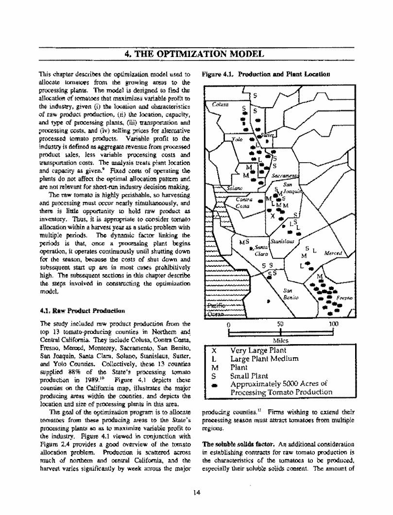
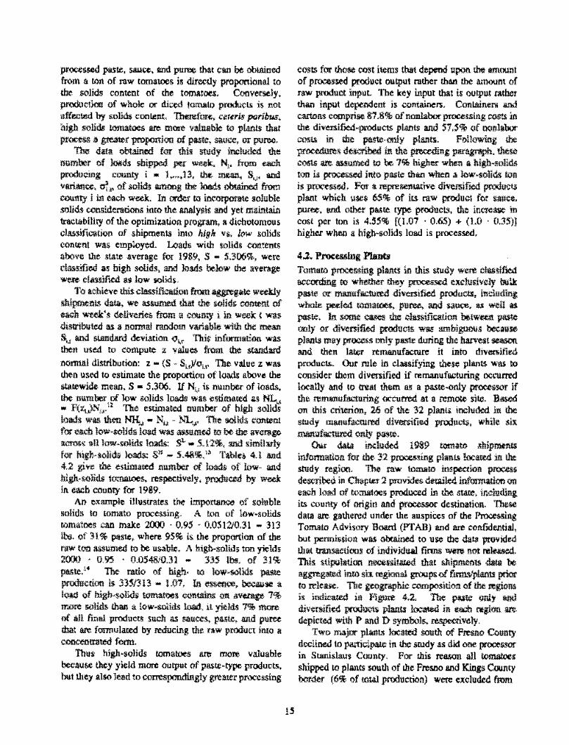
Tht srudy inciu;kd raw product production from lhe top 13 tomatc;·producbg counties in Northern an4 Ccnlral California. They include Colusa, Contra Costa, Fresno, Merced, Monterey, Sacramento, Snn Benito, San Joaquin. Sanla Clam, Solano, Stfll'lislaus, Sutter, and Yolo Counties. Collectively, the:>e 13 rounties supplied 88% of the State's processing tomaio prodecton in 1989.'~ Figure 4,1 de;licts the'ie t{lunties oo the Califore.ia map, llfustrntcs the majcr producing MCtt$ within the counties. an<l depicts tlie lcx;atk>n and sire of p!OClming plan!ll in thti area,

The goal of the optimization program is to allocate tooit<IOOS from ~ producing mas to the Stirte's process:mg pi;uw; so llli to m;uimi:te varialm: profit to the induMcy. Figure 4.1 viewed \n conjunction with. figum 2A provides a good overview of the l\lmato allocadon problem. Production is sc11ttered across much of nonhem and cen1tal Califomia, and ihe harvest varlet. s!gnifitll.nlly by week across lhe ma_i-Or

liigure 4.1. Productlon and Plant Localian

s t'AJU!ll

~ s • ••• •

x Very Large Plant L Large Plant Medium M Plant S Small Plant • Approximately 5000 Acres of

Processi1,gTomato Production

producir:g roontieit" Firms wishing to extend d!elr pr~ssing season must attra~ tomatoes from. multiple n:giom'..

The- soluble .sollds fact(Jr, An addition.al .oonsideration i11 est11blishing contracts for raw tomato production is the characteristics of the tomatoes to be produe-ed, especially lheir solub;e soiid~ conft-ltt. The amount of

14

processed pi.ISie, sauce, e:nd puree that Cfl:.fl be oblttlced fron1 a ll)U of rnw tomawes is directly proportional 10 the solids content of the tama1oes, Conversely, productXm of whole or di;;;ed tomato produ<'Ls is not affected by soli~ cooLent. Thtlrefmt, cettri5 paribus, high soli& tomatoes are more '<al:uable to pl.atits that ~ 11 gteMtt 'JX'l>P<ITTiOO of paste. sauce, or puree.

11w data obtained for this study included the numOOr of loods shipped per week. N,. fmm each producmg county i "' l,.'",13, tht. mMn., S,,, and vflri.Ance, or" of solid; among the 1ottds obtained froel C<)Urtty i it! each wu.k. In order to i:ne"orparate soluble solids considerations inco the analysis and yet maintain tract&biliry of the optimiz.ation program, a dichotomous class.ificatiori of .shipments into high vs, lo1<> solids ccmtent was emp:oyed. Loads with solid11 crnt~ents

above !he ~Late !;verage f<>r 1989, S .. 5.306%, were classifil'd a-~ bigh solids, and loads below dle average ""'ere c!ml"'ICJ u low tolkl$.

To achieve this classificatioo from ~ale we:ek.!y shipments data, we assumed that the wlid& content of each ....m's deliveri.¢$ ftom a coon;y i ln week c was dumibuted as a normal random variable with the metm S,; find sumdllrd deviation ;:i,, This infurmatoo was then used to compute ;;: value& from tbe standard normal distribution: z - (S · S,.,}lo,.,. The value z was tben used to estimate the proportion of loads above the statewide mean, S • 5.306. UN;" is numbec of loads, the number of low ;;oJids loads was e~tlruared ~ NL.,. .. F(1t,).."<,,.:i The estimated m1n1ber of h!gb solid~ loads was then NK.,, .. N4 - ~'L.,.. The solids content for cacll low-rolids load W1IS .mumed to be tbe average !lCTO!;;; ull low-rolids lruids: ~ • 5.\1%, and slmil:ufy for hlgh-aolidii loads S11 - 5.48%.1> Tahleb 4.l 11nd 4.2 gi¥e the esthnared number ti loads of low- and hl&Jt·Wlids 1roiawes. respectively, produccrl by wed: in each county for 1989.

An e:o:arnple illusrrates tM i:nportaJ'ICO of soluble solids lo tomato processing. A ton of low-solids tomatoes can make 20'.Xl · 0.9.S · O.OS1210.31 - 313 lba. of 31 % pl!Ste, w'here 95% is the propttrtion of the ru:w ton a:;sumed tu be usabk- A hlgh-solW;; ~on yields 2000 • 0.95 · 0.054810.31 .. 335 lbs. of 311,l; par;te.1• The ratio of bigti.. t(! low-sclhls paste

pnxiuction is 3351313 - 1.07, In essern:e, becai~ a load of higti..wlids tomatoes oontairui on avuage 7% tr.ore solids than a low-solids loOO, 1l yields 7% rttore uf all final product! such as &auccs, paste. and puree Wat are fomtulaced by reducing the raw product into a coocenrrnted foon.

Thus high-solids tomatoes are more valuable becaur.e they yield more output of paste·type produl'ts, hut I.bey 1.11$0 lead to ccnespondingly greawr processing

costs for thos.e cost items that depend upon the amount of pro::e~s.ed product output rather than the an1ount of raw product inpuL The key input that is output rather than input dependent is container.;, Conlilinern and cartons eomprise 81.8% of nonlaboc procc~sing OOIP.s in the divenif>ed-pro<:111ru pl'11lts and $7,5% cf oonlabot 001>ts in I.be par;w.only plan~. Followinz the procedures dw.:ribt>AI in the preceding p11tagraph, there costs a.re twumed IC be 7% higher when a hlgh-uolld& ton U ~ it't!o paste than when a low-1olids ron is pnxemed. FQT a rnpn:senwlve divemfred pr00ll17tJ plant whieh U$C$ 65% of Us. raw product for sauce, puree, Md other paste type producL~. the increase in cost per ton is 4.SS% [(J,07 · 0.65) + (l.O · 0.35)] higher when a high-solids load is proces~.

4.l. Procwhlg Phmts

Tomaro processing plants ln this study were clwislfied 11Ccon:.ting to whether llwy processed exclusively bu~ paste vt manufllciut'Ci! diVt:ISified productt, Including whole pu:led romaioos. puree, Md nooe. u wt:U u paste, In some C1UeS me climificatioo ~tween paste ooly or diw:nifitd produCls w115 ambiguous beeause plants rnay process ooly p.1!51e during the harvest season and then lat.er rtm&nufacrure it into diversified products... Our rule in classifying these plants was lO coosider tbem diversified if rernanufw;turing occurred locally and to treat them ru; a paste-only pr<>eessor if the rem1ntufncturing occut'!:'ed at a rem~ site. Based on this criterion, 26 of the 32 plant.> included .in die study !IUU!Ufacn.tred diversified products, while six nwti.tfa.:::tured only paste.

cm data im::luded 1989 tornatb s'hlpmants infonnatlon for the 32 p~ing plants located m lhe study regloo. The raw lomato in~pcalon proc<CSs described in ChapLer 2 provides detailet! infornultloo on each load of to:imtoes produced in the sLUC, including its county of origin and processor destination. Theliil data a.re gathered under the au$pices of the Processing Tomato Advisory Boani (PTAB) and are confxle.ntlal, but pennission was l:tbtaintd to use the datii provided !hat tnmsactions of indivklual firms weni not released. This -stipulation nec«sltai.ed that Ytlpments data 00 nggregQd inro si1 regional gr00pso! finm/planu prior to relell5e. The grographlc composition of the mgions is irnlicared in figure 4,2 Th¢ pute ooly &lid diversified produrn plants 1ocMed Jn e-OCb regixm a.re depicted with P and D symbols. respecrively.

Two n-.ajor pl&nlll locattd south of Fresno County declined to 1'<41'.icipaie in the srudy as did one processor in Sumislaus County. For !his reaoon all tomatoor shipped to plants routh of !he Pres.no and Kings County border (6% of total production) were excluded from

"

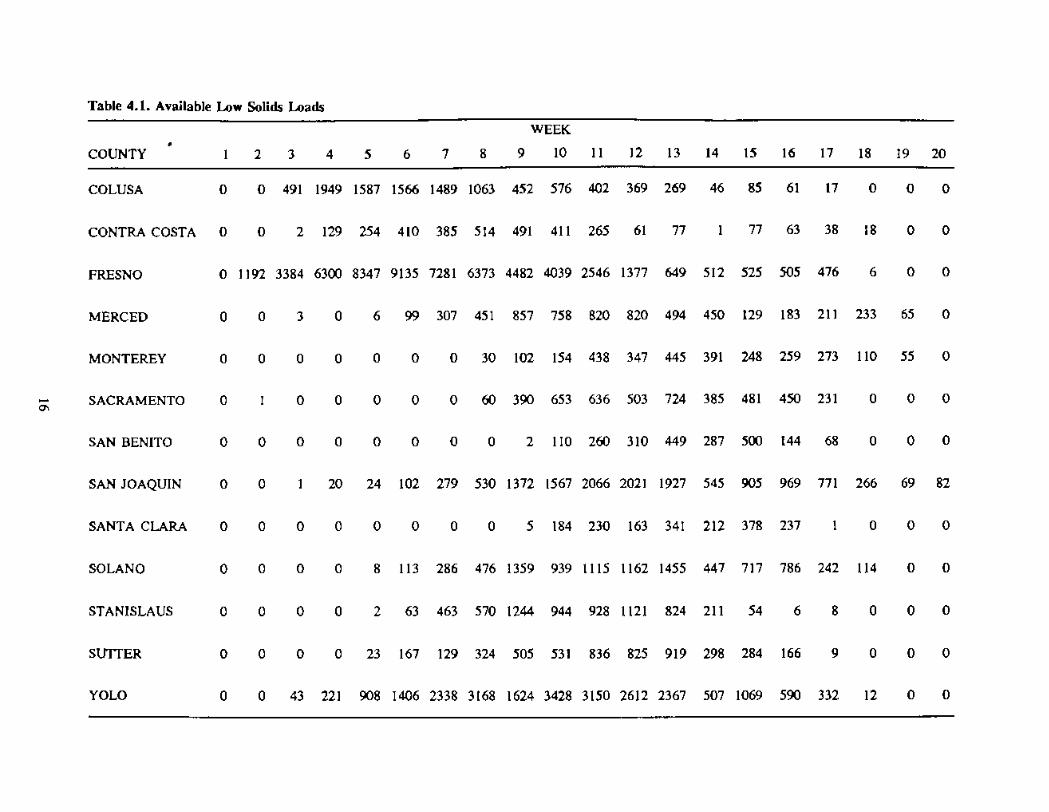
Table 4.1. Available Low Solids Loads WEEK

• COUNTY 2 J 4 5 6 7 8 9 10 II 12 13 14 IS 16 17 18 19 20

COLUSA 0 0 491 1949 1587 1566 1489 1063 452 576 402 369 269 46 85 61 17 0 0 0

CONTRA COSTA 0 0 2 129 254 410 385 514 491 411 265 61 77 77 63 38 18 0 0

FRESNO 0 1192 3384 6300 8347 9135 7281 6373 4482 4039 2546 1377 649 512 525 505 476 6 0 0

MERCED 0 0 J 0 6 99 307 4Sl 8S7 758 820 820 494 4SO 129 183 211 233 6S 0

MONTEREY 0 0 0 0 0 0 0 30 102 154 438 347 44S 391 248 2S9 273 110 SS 0

SACRAMENTO 0 0 0 0 0 0 60 390 6S3 636 S03 724 38S 481 450 231 0 0 0

SAN BENITO 0 0 0 0 0 0 0 0 2 110 260 310 449 287 soo 144 68 0 0 0

SAN JOAQUIN 0 0 20 24 102 279 530 1372 1567 2066 2021 1927 S4S 90S 969 771 266 69 82

SANTA CLARA 0 0 0 0 0 0 0 0 5 184 230 163 34! 212 378 237 0 0 0

SOLANO 0 0 0 0 8 113 286 476 13S9 939 lllS 1162 145S 447 717 786 242 114 0 0

STANISLAUS 0 0 0 0 2 63 463 S70 1244 944 928 1121 824 211 54 6 8 0 0 0

SUTrER 0 0 0 0 23 167 129 324 sos S31 836 82S 919 298 284 166 9 0 0 0

YOLO 0 0 43 221 908 1406 2338 3168 1624 3428 3150 2612 2367 S07 1069 S90 332 12 0 0

WEEK

COUNTY 2 3 4 ' 6 ' • 9 10 11 12 13 14 15 16 17 I& 19 20

COLUSA 0 0 289 2018 2694 1478 1474 795 326 517 643 679 462 14 34 0 0 0 0

CONTRA COSTA 0 0 78 444 666 60S 387 420 225 70 29 43 58 0 20 Il 0 0 0 0

FRESNO 19 1733 6069 &541 9050 7477 6154 45?7 3293 1683 S17 651 363 87 69 129 126 10 0 0

MERCED 0 0 19 0 2 24 203 621 1129 681 596 382 196 169 26 14 47 33 3 0

}.10NTEREY 0 0 0 0 0 0 0 0 27 l2S 95 67 34 37 11 13 24 ' • 0

SACRAMENTO 0 0 0 0 0 0 0 27 203 537 469 363 316 202 113 109 62 0 0 0

S.-'1.N BENlTO 0 0 0 0 0 0 0 0 54 320 754 706 696 298 393 85 ' 0 0 0

SAN JOAQUIN 0 0 0 61 9J T9:i JS! 501 !212 l l7t 1292 1492 1216 404 539 295 155 36 0 2

SA."ITA CLARA 0 0 0 0 0 0 Q 18 75 187 t93 1()7 148 78 9Q 116 0 0 0

SOLANO 0 0 0 0 ;4 102 41 ! 446 1582 900 8% 848 872 197 :528 528 134 0 0 0

STANISLAUS 0 0 0 0 46 271 699 675 JOi3 520 585 623 543 119 67 19 4 0 0 0

SUTIER 0 0 0 0 17 404 9JK 1212 2069 2377 2469 20!5 1726 8.34 535 ' 0 0 0

YOLO 0 0 30 6S4 2292 3302 37a1 4042 N78 3627 36R3 3450 3126 608 1034 272 51 0 0

••• ••

~Fl~KU;::::''::.;:'·~'~·~l'«<~="'::'.''e•<!:.!R"''gl0o~"'?'"~:::~~-:t - 1-[ D

P D

Miles

-

'·.•••• ,,,~,Iii/

2

3

4

5

6

•

D P •

Diverse Plant Paste Plant 5000 Ac:r~ (appro:<lniately 150,0CO tons) of Processing Toniato JJroduction

rhis su1dy as were the tomatoes shipped to the StAnlslaus County processor (3·5 p11ret.1nt of total production in J9&9). Finally, a s:nall amount of production ~hipped to vegetable freezen and dryers wu a.loo e~lud«l,

The processing pkmtS< irtehlded in the $tW!y, i.belr location, processing reg!on affilla!100, ~ type, and estimated weekly capaclty Me llslcrt in Table 4.3. Pl&.nt capacities were emimated from a number of s~ and oonfumcl with irdustry el!perts. L"l general, capacilies o! the various pla.i.ts are well k;n(!W!l dlroughout ihe industry, and we do not treat our e~ti1nares as confidential.

F.stimaies of annual production Jn a plant earmot be translated directly into an e.111im.iue of tt.e plant's

weekly processing capocity. Typically plllll~ operate at full capacity during the height of the hlU'llest season and at lesser rates early and l&te in the seawn. Our estimation of weekly eapw::ities for the vari-Ous plants 1ook into act-OUnt the !l.ggrega.~ weekly pro.,"l)Ss:ng volume ob;erved during !he s.easoo and general knowledge regarding plant char&cteristics and scheduling. Specific fucron considered in establishing weekly processing capacities ~'ere (i) tr.e volume of aggregate feU WC>;lkdeliveries-approrimaiely 7.8% of ili'IM.ll delivcr'.es, (ii) ti;c ol;:is.etvatioo that small plants genemlly operate :or fewer weeks tl-.:ut larger p!&nts and (lii) the volume of wral weekly And annual ~hipments to each processing region. Based on these factors, small. mediurn, large, and very large plants were assigned weekly cb.paeltles of 10%. 9%. 8% and 7%, teSpectively, of their ;mnuul processing volurr.e.

4.J. T~etion and Pr-OCessing Cast&

TrID!sporta.tlon ;;osl$. T<1ble 4.4 provides estim.ai.c<l ~portmion mi!c!ge from each producing county tn the California cities where pma:-ssin.g plants are located. These es:iniaies were derived by the authnfli based on the rwailabl-e transpDrtati0t1 network and the approximalt location of production in each c-0unty11 . TranSp<'.lrt&ion co~ts per too, TC, for Clich shipment from 1:0\lnty i to plant n were caL."lputed us:ng these =nlle.ages, D,,., according t11 the formula:

Prtl<'t.mng ctKts--divenified-produ.:ts plants. n:e optimization mOOel reql.lire$ csti:na!es Qf pl\)OO!lsing oo;;t~ fll'f both pa$~ a."l.d diversified plants, Our primary sO'.tt~ for diversified plant co~u was the study conducted by Losan (1984). Logan obwlncd labor and nonlabor COiltS for a moderute-slie divers.ified·producw plant in California. The pl.ant operates 12 canning E.nes, 7 of whicl". proces;_ only whole wmaroes, a."ld 5 of v;hicb ~; either sauce, pnree, or pasll';, Production !lexibihty io the plant is obtwied by (i) Y3l}'ing the number of canning lines \n operation, {ii) operating from ooe to three eight-hour $ifts. artd (iil) q>etacins; from five to seven days per week.

Logirn developed a rompwer n:ode: ro select the lease cost mode of operal;il;in, given the amount of raw tolllltooS arriving weekly and mMagemcn~ priorities on the processed prod1Jct pack. Logan's analysis illustrates the nature of short-run operating roon.omif's that e~ist it. che indu5tl)'. He writes {p. &):

"

Teble 4.3. 1939 Plants fttld Estimated Wildd} Capaclll~

Tri><' Wilclcty

(;""'• ......, c-FlrmN- Locativn D•Dlvene (000 kins)

Colusa County carutlog Co. Flatter Packlrtg Co, Pacific Coosl Produ;;:ers

William~

Oroville Y'Jba City

p D

D

17,5 17.5 12.0

2 C6ntadl:na Foodil, Inc. Bt:titrice/Hunt·We"40n, Inc. Dixon Canning Co. (Cambell) Amerkill\ Home Food Products Campbell Si>up Co. Sierra Fniit Co., Inc.

Woodland Davi$ Dixon V&CZviEe Sacramento Sacrammtto

D D p D

D

D

40.0 36.0 17.0 27,0 I 1.5 13.5

' Heinz U.S.A. &int U.S.A. Tri:Vallc)' \.>r0wers Tril'lI'll.Icy Growers \'ailey Tom$0 I'roducls,Jnc, {Qunpl.X'.!l) Paci.'i.c Coast Producers Ragn' FOl'X!s, Inc. Qua.'ity Assured Packlng, lnc.

Stockton T~y

Stockton Thornton Stockton tool

'""'""" Stockton

D

D

D D p D

D D

27.0 49.0 20.0 20.0 25.0 12.0 27.0 115

4 Be.atricC1Hunt·Wesson, Inc. Del MOnU:: Corporation

Escalon Packers Tri/Valley Growen

Oakdale Mo:le>.:o &raloo

"""'""'

D

D

D D

4il.O 31.5 7.0 15.0

Gangi Brothen: Packing Ce.. Garden V~Uey Foods, Inc. Gilroy Car-"llng Co,. San Benito Foods Sun Ganlen PlK'king C°' Tri/Val!e7 Growers

Santa/Clara Gilroy Gilro)•

Hollister San lo:ic Hollister

D D

D

D

D

D

13.5 l l.O 135 1::t5 26.0 15~

6 Atwater CllI!ning Co. Jngomllf Packing Co. Ragn' Foods, Inc.

TOMA·TEK, lnc. Tri'Valley Growen

,\1waw Vol:a M.er;:ed

I-ltebaugh Volta

D p

D p p

14.S 27.()

37.S 20.0 34.0

"

Table 4.4. TnwpomtioA Mileage from Produdeg ltt:gion:& to Proces5ing Pl.ants

COUiicy CO'Ju2 S:utlu sm: Solano umtr.l -,,,,.,~.;;--g~.,,,--,K~tiii=~--.y~ii!O"-'Siii=--,sffion=•·-M""'~~@::r-p~==~oc

City mt"nl!J Cost\! aara Benito en:y Joaquin slaus Oroville 7f 49 14 9(t 142 202 245 273 SJ 116 162 205 275

Yuba city 50 " 35 94 '" 167 210 238 .. " 121 170 "" WiUi;un$ 17 49 59 " 138 "' 21l2 230 51 l<lS IS! 194 264 33 31 19 41 119 1.. 1'3 "' IO " 111 154 "'

""'" 44 42 30 30 "" "' rn 100 IO " !OS 151 221

DW,,, '2 46 " ,. '"' "' "' 196 10 66 112 155 "' Vacaville " "' 41 "' 86 107 '" 1'2 25 l!2 '" Pl 241 ,_., " " IO " ,., 167 "' 25 42 " Bl 201

Th~tun " " " 30 " 115 142 166 p 66 104 176

LOOi " 7l " 2S " 113 140 1"1 57 10 .. 102 174

Stockton 102 " 60 J7 24 94 121 "' 71 24 45 83 '" T=y 123 106 81 30 73 100 162 92 45 " 69 152

°""""' 134 111 " 11 58 108 12' 133 105 "' " " " M"""'"- "' 125

112

11"' " 74

66

62 " 49

103 ,. 116

!16

lW

112

100

96

34

3S " "

" SS

75

" SllII Jose 139 146 '" 106 152 ,. .. '"' 99 111 "' 153

Gilmy 169 176 167 136 100 23 28 67 "' 136 79 " 127

Santa Clan 151 146 131 106 "' 15 " " Ill 99 111 134 159

Hollis let 184 191 1'2 151 !IS 23 10 66 148 132 75 SI 123

-- 154

"' 131

IJI

112

1()6

99

93 " ., 104

"'' 90.. 148

"' 123

113

67 .. "

36

" " " Volta 185 "' 143 92 116 74 60 117 154 1111 " JO 69

210 193 "'' 145 132 1'13 .. 146 !79 132 " " "

Muoh of the direct labor required in tomato proce$sing operations is more or Je~s con$t:ant regardless of the rate of output. For example, moo! of the labor needed in the recciving all.d general prqmation C!p!;':rl!tions, the general pro;;es$lng operations, the general service functions, the bri~ \tan) s111tking, cooling, and f'mh;hcd pack receiving ope.nu.iOl'l$ remllins eS!ie'lltially unchanged no n11.1111:r how mw:iy canning Imes are being opttattd or what finfil produ.:ts: are being produce1.t In conttast to these labor economics, nonlaoor

inputll such as cans, canons, energy, water, and various food ingredienu; such as salt are added to the raw t.omato input in approxin111lely fixed proportion5. Thus, we oonsidered labor and nonlAbot oosls separately for bot.1 divrnifi«J prnducL~ and pasle ;>lanu. Non1a?or cootll in either rase V.'Cre treatci! :u a cooswit amount per nni: of raw tomatO procased-

Lat!an's labor l!nd nonlaoor COM& were updatci! to reflect prices in our base year, 1989, trpdaood costs by item are provided in Table 4.5

Table 4.5. 1989/1983 CQ!it Ratios for Dlvmilffed-Produets Plants

Cost Item 89/8~ Cost Ratio U.boc t.122 Electrir:ity \.424

0,9%G" Lye L092 s.i, l.118 CaM l,lt9 a.n~ 1.149 Boiler start up 0.996 Evaporator clean up 1.139 Water l.092

Sources: Clilifornia LaMr Market Bul!etlu Slatirtical. Supple1nc:rt lml3, 1989 (labor rott}, Bweau Qf Lab<!r S!atiltk:.'>. P'rodni:er- Price indeJ; 191!.l. t%9 (elewklty, gas, lye, mtli. ~ ~s), a1:li1 ~ of Wi.w:t Re~ Bulletin t32-$9 (w~),

Based upon these price change>,, oonlabor variable costs per ton ~'ere OO!Iif"Jied as indicated ln Table 4,6:

We also needed to o:ixtrapolare l.ogan's anoJysis to estimate processing costs for larger-size diversified pl&nts. Given updated labor cof.ts, Logan's optimization model was re-rur, t.o establish the

Table 4.li. Nonlabor lnput Costs per Raw Ton: Divenlf'led-Producu Plants

Cott lte.:1n Cost<1mv"'$olids Cost1bigh-solids

"" ""' electricity Sl.97 un

""' 10,32 li132 ,,, 0,9$ 0.95

water {).41 0.4:

,., 1.67 !.75

'"" 99,97 104.52

CarlOl'IS 6.56 6.86

TOTAL 121.85 126,78

minimum labor 00it5 for processing weekly vOb.lme& up to 13,00J rsw tons per week, the capacity of Lat!e.n's base plaru. Capacity within a divernified-pnxlucts plant is increased by addlng addh:Jc.r.al t'mming liner.. To esUma:e costs of QPC:ating additional lines. labor oost:s l!Ild i::lean·up costs from Logan's analysis were modeled as a function of the nu111ber of line$ and shifts operar.ed per day, 1·12 and 1-3, rer.pectively.16

To i:s:timate thei;e costs. for larger plants, JA.bor and c-ka.,-up oost per day were cornputo:I for alternative opert1tin@; n:;gimcs in LJ:.gHn's base plant. These roots were then modeled as a llnew function. '1f ftrtt tl!ifis (S11 adrlitiorutl shif'.s (SA), and lines tim~ total shifu (l.S·S'I). where ST-Sl+SA, cperate<l in the ba!le p!Mt: (4,i) tCi, .. b,(S !} + b,(S,\) + b;(LS·S'I)

Thi$ regression equation \¥as estimated with the data obtained fm1n re-ninn\ng LJ:.gan's model whh updated cost it1f0nt1ation. The estirr1atci! equation ww;

(4.2) LCri .. 28076(51) + !.6546(SA) + 680(1'..S·ST), R1 ...996

AWJ.ougn LJ:.gan's model :iao different operaling rareo for different liOCfl, it was usun:ed that th¢ product mix w11.t oo:istant, g1:'1'iog an average of 72.9 raw tvni;. processed ptr line IN'! shift. This volume was th!::n uted to estimate the munber of canning lines needed to obtmn alternative weeil} p~'ng cap:i.citi$. We t:&timated lalxJ: and clean up costs f.or plants with 18 !im:g (27.5 th!'.JU~d ton week.iy capacity), 24 llnes (37 thousand tons per week), and 36 lines (55 thousand tons per week) using equation (4.2). In addition to direct Cos.t increases from additional lines. operai.ed, shift labor co~ts (primarily for supervisory and

•••

receiving functions.) were estimated to increase by LS% relative to Logan'5 base plant in lM 27.5 thousand ton capacity plant, 30% in the 37 thousand ton plant. and 60% in the SS tho;isand ton plant. These adjustments reflect 1-Jgber managerne.'lt costs in :ill'ger plants due ~ii.her to higber·plliC: manD.gers m" :nrne managers being hlred.

Given this extrapolation of l--0gan's analy,f,; to

w:omi.ruxla\e larger -slze planm, the fmal srep in the process of deriving di•~ifidi plant labor and ck.art up costs (LC) was w estimar.e the relationship between IX.est OOSU and !(Ins of raw tomll:loot processed (TONS). This rcia1ionship wa$ obtained by fitst deriving the minimum labor and clean up cmt <.:onfiguration for processing alternative rsw prcxluct tonnagl.".s in either Logan's base plant or illi 13.l'ger analogues, And then estimating a log Ji.neat average c0>0t fur.ction: (4.3) :.U(LOTO""J - a+ i)ln(TONS), Oioii.X of this functiooal form w,as dicta~d by the nature of the operating e\..'ffi10f!ries 11ppmmt in the data "' tlluitmt&I in Figure 4.3. Tiw estuna!ed functior. was: (4.4'1.) ln{LC:TON) - 7.564 - 0.42 lr.(TONSJ.

R2-.921

(4.4b) LCJTON - 1927"5"TONS·~1

l'he estimated C1.Jrve is depicted in Figure 4.3.

~Ing ttisti··paste plants. Production ;:;-w. da.ui far a moder.ite--size (150·'200 rhwlllll'.d ton searor.al capacity) paste processlng plant w.o:> ohtairted and provided the baSic data input lnto estimauon vf paste plW pro::t:sfilng costS. Ptiste plant& prov'.de a product wgeood lit other food manufl<ct\1(1.11'$ as an ingredient. Bulk pure is umally packed mw SS or 300 gall-On conw.\nern. Mult:ipie canning lines &."C not operated as in diversified·producrs plimts, and, hence,. paste plutts lack some of the operational flexibiliry of adivtmified-producr.,, plant. In particular, once a paste plant begins operations, it is usually roonomical to continue operntio:ii;, 111 fu!1 capacity i:hrougbout the processing season. 1 ~ Thus paste pl(t(!l!i will cypically oper:rte

three ;,hifu 11nd run :.even duys per week thrmtghoot the processl:ng season.

Similw to the dive:i;if>Cd-products case, it was a::M:ful to separate labor and nonlaOOr proce&Sing ;:osts fur paste plants. Nonlabor cost; include Cl.l$1& fm' energy, W.1>1.tr, ~upplie&. ingt'reJent\. ar.d containen. It once agfiln ls, reasonable to assume th.at energy, wawr and snpplies are used in fixed p(l)(X.lrtion to thi;i volume of raw t<:tm~toos procesSied, and, therefore, that nonlubnr coots are consLmt µer unit of raw product

Figure 4-1, Olvenlfkd Plan:t Ave111ge- Labor Cost Curve

• ·····-: • •

' '

pruce$sed. Container cosu iOCiealle in proportion rn Lie solids content of the raw tomato. E~timated costs per too for !bose items !Ire indica!Cd in Table 4.7 The contl!iuer wsl cakul111mns assume Wat 19'4> of each raw ton is pt¢k¢d in S5 gallon drums and tht ~ in 300 pl. cartons,

Tabl\l< 4.7. Nunlabor Inpat Costs per Raw Too: Paste Plants

Cv.,t itt:rn Costilow- Cos1/high-solids ton solkls ton

elecoic.ity $1.89 $1.89

"" 3.19 3,19

supplil.!S 0.64 0,64

SS gallon drum 6.19 6.62 (19% of each ton)

300 gallon carton :.70 I .!i2 (St%)

weighted averuge 13.61 14.16

~ww of the contim:ous nature of pure plant operations, lal:Jor..crut economies arc even more pronoonced In paste plants th.tn in diven.ifi«l·product$ plAlll!i, Once a plant begins opcrntioos, labor CIJS!s a.re essentially fixed wilh Nspect to the vnlume ~sed. so the .!lV\'!tllge labor cost function approxlro11tes a ~g-Jlar hypetbola--it declines rapidly and then levels out fox large processing vohirnes, To acoommodate the diffi::rent ;;:~ity levcis of Califomia paste pla.1.r.,,, we estimar.cd labor costs for three different capacity pil.'lte plants: 18,000 tons per week (the base

22

plant), 27,0C() wns per w.eek, and 37,0C() Ions per week. Costs for the largcr..¢.llpacity plani.s were obtained hy adjusting costs for the bare plant in consulta.rio.'l with industty experts.. It is cvrnmool)' acknowledged that substmtia: ccooomics of sll.C cxi~t m paste plant openu:ion. F¢r e:umple, ooe apert $U~ that a doubling of p!!ll'lt capaclty caiued labor OOS1S lo rise by only about 15%. The estimated empkiymcot requirements and wocia!tld oosu; fur each plant are sum.m!Uized m Table .Ut

Giveo the eoonomics of putt; processil'l,!h a paste plrml lncnl$ full !abor C\'.IS!S. C"', per week if it is operating, e.g .. c• - $82,!35 per week fM the plant with 37,000 raw tons per W«k capacity, and csreDtially 1ero direct labor costs if the plant is not operating. This lyp!t of disoontinuous cost f.inct!on caused problems for the nonlinear nptimizatlon compucer routine ni;ed in the analy!iis. As a C-Of!illqll(mce, the labor-cost !'unction was "smoothed" by er:1pkiying the following trar.<Sfmmrillon: (4,5) LC' .. C*{t • e-•n:ms), where k. is an appropriately scl«!led parameter. Thls functloo asymptotically approach.ts c• 11$ TONS pr~sed bKomes large. The larger is the parnmcler k, the fa~J.er Ld' approaches its azympt-Ote. Therefore, by setting a high value for k we were able to preserve the reality of operating economics in paste plants while maintaining a smooth labor <:Mt f.inlltion. Figvre 4.4 lll\lsr:ta!t:s the LC" F ton functioos for !he base, medium. and large psste plg_i:;.

F1gun: 4.4. A.n:nge Labor Coot Cunes fnr Paste-l'l j

I

I " l ""

4,4, J>rocesiw;d Products Output To :::omp11tc vllriable profit from tomato ~sing, we needed lo make assumptions about the types of processed products being produced. The outp11t mix, of Cttlll'S¢, differs. for eeth diversified products plant.

OutpUt dtvel'liit}' for pMte-only planlli is reflected primarily in rerms of the bulk container choice.

Each firm's product mix is confidential, so the :altemative purwtd here wa$ to assume that the final product breakdown foe our ba~ diventfied·produi:!ll a.nd pas:.e plM't!i held acrO.iS all similw: plams}' 1be divusified·pr0011(1$. plw in Logan's study produced three can sites of whole tomlltoes m:d p!Ute, and two can sizes of puree and sauee. The allocation of final products {by product Md can size) for eath row ton in !be Log!tn base plant and the 1989 sel!ing price are su.rrunarlzed in Table 4,9. This proasood product breakdown was used to cvnsnuct a composite product to establish the "alue of a ton of raw lom111oes processed inl.O diversified products. Since Logan's study includes no information on solnblc ~olids, it wu aswmed that the volumei lhlted Jt ·rabk 4.9 applied to a low-solids !On of :omaioes. Carrying: oot the computations from Table 4.9 yick'.s $355JO at the FOB value of a low-solids ron -0f IOmalOes in r.1w product forn1 ln the l:ra$e yeM. About )5% of raw tomatoes in the b&!ie plant w~ u!ioed IQ produce whole tomato products. Thus, the value of a high-solids too was $355,10"((1,()7 · {l.65) + (1.00 · 0.35)) .. $371.26.

The same procedure was used to create a eontp-OSitc paste plant ourput 'The base plant produced 19.04% of a 55 gallon drum and 6,96% of a 300 gallon ;:&ttOO from one ton oflow·oolids tomatoes. Give.rt 1989 paste prkcs, the FOB value of 11 low-soEds ton p:ocessct as bulk pauc Wll?. $181.80. A hig:i-wlids ton was ~i!'!gly worth :Sl8i.8 · lfil • SI94.53.

4.5. The Mathemalkal Model The mathematical programmi.:ng moCel to determine the optlmlll a!i(')CAflon of r.aw tomatoos from northern and central Catifomia producing counties to prooessing f11Cilitles consisted of the following coniponents:

(i} Tou.I openuing ~s per week t, TC., at a diversified produru plane j.

(4.6) TC/" 1927,5 L" ~,,XH,;F n

,, 1011.20!: <X4,l + 1.oillXH.!I

13.65 E" (XL,;+ XH;_\j, i•l

j = J•• .,,26, t = l,. . .,20.

"

Table 4,8. Labor ia Small, Medlum, JUMI Largt" Paste Plants

Job Function $!Mm II Emplo~

Small PJ.m! Payroll/

st1ifl"

S@ium Pfu'it

' Payroll! Employ.i Slufr

, EMployed

Large Plant Payroll/

Shift Gm"!' Lwk< 13.82 0 0 0 Q 0 0

Meclianic A 12:.18 I 97.44 l 97.44 97.44 Mechanic B l j ,00 0 0 0 0 0 0 lns(rumeru/Elecirician 12.l!I I 97.44 97.44 l 97.4'1

Boiler Opera1or 1'2.:8 I 97.44 l 97.44 I 97_44

Raw Material Opetalor 10.00 Q Q 0 0 0 Q

Yard Truck Driver 9.68 I 77.44 2 !54.88 2 154.88 Tomato Unlooders 8.18 I 65.44 I 6.'1,44 l 65.44 Flume Artelldlult 9.00 2 144 00 2 144.00 2 144.00

~ ~ Sorters 8.18 6 392.64 7 458.08 8 523.52

Clean Up 8.18 2 130.88 2 130.88 2 130.88 Tomah"l Preparation Operator 10.00 &'i.00 85.00 I &5.00

EvaporaLOr Operator A 12.18 109.62 101.53 I 103.53 Evaporator Operntor B 11.00 88.00 9:8.00 I 88.00 Filler ~ Weigher 12.18 6 584.64 7 682.10 ' 779.52 Fork Llft O,p(rat<Jt1C0J11<tiner Handle1 9.68 l 232.32 l 232.32 3 232.32 Clean Up 8.S4 L 68.32 !.. !l!LlA. L 68.32

II of emp!oyee~ishifi: " 31 33 SUBTOTAL $2265 $2,504 $2,668 DUv;t laW i;Q$t$/$hift 3,008 3,393 3,613 Dllte1 Weekly Payroll 64,432 7?.246 75,863 Direct L.::tbur Cusl/Too @ Peak Capacity 3.58 2.44 2. l l Total Weekly Payr;:::ll (n:ccivlng clerks & lab tetJuocians :!Jded; $70.704 $77,517 $82,135

• Jn;;!~~ overtime lf any.

Table 4.9. Processed Product Production for Diversified-Products Plants

Product type Can 51ze/cuse

Whole tomato No. 303/24

Whole tomato No. 21/1'24

Whole tomato No. 10/6

Sauce & puree No. 10/6

Sauce & puree No. 21/1'24

P~re No. 6/48

Paste 12 oz.124

Paste No. 10/6

Number of cons produced per ton

231.89

96.79

25.14

13.96

18.10

256.90

82.89

3.25

1989 pricel$ case

8.75

13.50

12.50

12.25

12.50

13.00

12.35

25.00

The first terms in (4.6) and (4.7) measure laOOr costs, the second terms measure nonlabor costs that are proportional lo processed product output, while the third terms measure nonlabor costs !hat are proportional to the volume of raw product input (!ICC

Tables 4.6 and 4.7 for derivation of the nonlabor costs for diversified and pa.ste plants, respectively). In (4.7) AE' is found for small, medium, and IBrge paste plants on the OOrtom row of Table 4.8.

(ii) Total operating costs per week t at a paste plant k.

(-ioof txLu'•xn..:iJ(4.7) TC/•AE'I-e[ "'

" + 1.89 E cXL,.~ + l.01XHi.~>;., "

+ S.72 E ,., CXL..~ + XH;.~}.

k ~ 1,.. .,6. t = 1, ... ,20.

(iii) Total transportation costs per week, TIC,. toa processing plant n.

" (4.8) TIC,.=E (XL,.~+ XH,,~)((O. lO)D1" + 5.00),,_, n "' 1,.. .,32, t = 1,.. .,20.

(iv) Weekly total revenue from processed product sales.

. " TR, =PDE [ECXLi1 +1.0455XH;~1)J

(4.9) j•l

' l•l

" +PPL [E(XL,~ + 1.07XH,~)J, ); • ' 1•1

t•l ....,20.

Variables in !he optimization model are defined as follows;

pD diversified processed product value per ton of low solids raw tomatoes

P" paste product value per ton of low-solids raw tomatoes

XL,,~ Tons of low solids raw tomatoes transpo~ from county i to plant n in week t

XH;.~ Tons of high solids raw tomatoes transported from county i to plant n in week t

D;" transportation distance from county i to plant n as reported in Table 4.4.

AE' laOOr cost parameter for paste plant k

Combining !he model components (4.6)-(4.9), !he full optimization model can be wrirten as:

The base optimization medel is subject to lhe following constraints:

"

•••

{4.10)

tt ' nIl, •1ll,-LTC/-:£TC/'-L rrc,". ;•: •~1 ,,.,

t ,. 1,...•20.

(i) A Fki.itt n <.:11.11UOt pr~s mOf'e tonnage !him it!!i weekly capacity, C' a& imlica1ed in Table 4.3.

(4.tl) Eu

<XL,: - xa:) s c ~. "'

n=-1, ... ,32, t"'l,,... 20.

(ii) A county i cannoi supply mart low-solids tmtnagc tl'.ll!l lU l<"N·solids tomato prOOuction, prnrluction. t.'Ll' in Illy week t, as reported in l'able 4.1,

" ' (4.12) E XL,! +L XL,,~ 5 NI.,,,. J•i ....

i • l ....,13, ! - l~..•20.

(iii) A oounry i cannot !Wpply ~ higl:.-so'Jds toonage than its high-solids tom aw produ\'tion. :'.'.'H,J in any \11«:.k I, !lS repor;etj in Table 4.2.

"" i ~4.13) E XH,J + E x.tt; s NH,,,

f'\ •••

i"'[,,,.,J), t"'l,n.,20.

Observe that formulation a."ld Y\lution of the base opllrn.i:r.atioc model docs not invclve use of the confidentutl f>TAB inspectioos data on W\'lcl:ly shipmenrt from prnrluClng counties to iudividulil pr~g mgioos. This infomm:lon can be incorporated into the program as addiclonal constraints that fQl"t\e the solution ro approXilnate tl:e actual 1989 allocation, The optimal oolution and the constrained-optimal solullon can then be compared and evttluaood, The specific constraint that furt:es the (eotimated} acrJ:tl allocation is lhllt:

(iv) the to:al raw tomato tonnage allocation from couruy i to all pla..'ttS j - 1.... ;R ir.. each processing regioo r must equal the aotu.!ll tooru.ge allocated, AL~, to the retfun for each week t.

' E (XLJ. • XH/J • AL,;. '"

i•l,.. ,.13, r~l,.,.,6, t"'l,.,,,20.

A less remlctlve venion of U'Js coruitraint ls. to rnqum. only that:

(v) the total allocation to .a region fron1 al'. counties i - !,...,13 nmst equal the lld.1.lal allocation to the region based -00 PTAB m:QtdS.

• u («15) EE (Xl,j • XH..{l •AL;.

J •I ••I

r=l,".,6, t,.1, .. .,20.

The base model, equation (4, 10) subject to (4, 11 )-(4.13), was solved as a static, mu:ti.period problem using the nOnlinear optim\ZAtian program OAMS.'~ This solution procedure dOC1 not incorporate: cl.re dynamic~ that link weeks in the pr(l(:Cssing season, namely !h\i! pm¢t$$on: rem11in irt contmvotis ~ lhroughoot their processing SeaIDn$. This >:oosldtoration can be inw.xluc-«1 explicitly iruo the program by defining Jnieger variabl.es E,,l M follow:.;

u (4.16) If E iX4~ •XH.:) >o.

then 8': .. 1, otherwise &:' ""0,

n•l,.n,32, t .. J, ... ,20.

The conse-.-uuve operations oonMraint can then be lmpo~ed $ follows:

(4.17) If 6/ .. 1 Mid&.,, -1,then&,.1 .. I.

To incorpornro this constraint, a base pcriOO t* must be established for a:J plants n where ff',. - 1. For example, t"' cauld be tlesignalfd a& tl'.e peak delivery week in a given pro;:esWng season. This procedure could be repeated by cbool>ing different hate wee:ts and ll"enluallf selecting thit oolulion set !hat achieve~ the highest variabl\l pmfit. Fortunately. in our applkatioo of the prognm.-ning model, the consecJtive '<l/tt\ks. oper.u:ion constraint was mtt ti.e,, the cor..strain1 was slatk} by Jlmost nil plan« in the base &0lutiO!I w the :nodel, thns vitiflting the need lo rasort ID che integer eons!raints described in (4.16) and (4l7).1c

5. THE BASEll-fODEL SOLUTION: OPTIMAL VS. ACTUAL ALLOCATIONS

T:-!is chapt.er presents results for L're base opdmi:u.tion model described in the prior chapter and compares che op!i:m& results to solutions. obtained by conslt'aining the bate model to epproximate L'>le actual allocgtion. The ~year for the analysis is 1989, Ir. eMCrtCC the b&e op!i('f)).ialioo proQkm is to allooaie the loads of too:lJliQe$ rontained in Tables 4. I and 4.2 to the :m;cc.s!iing plants with the seasorutl capacities r.cted in Tablt. 4.3 so a.~ ro maxirnin: variable profit to the industry. 'file malhematical problem is expressed as equation ( 4.10) i;ubject to constrnints ( 4.11)·(4.l 3).

Imposing constraint (4.14) on the model produces what we shall call coMrralned made( A. 'Th.i$ allocal.ioo requires each proc.essing region to ~ive its acnaJ weekly a1\ocat:.or. from each coonty bast'-0 on PTAH recon:ls.. Com~ alloctrtton A i$ thus an emimate of the actual &Jlooatioo of tomatoes to oorthem and cemral California proceMing plants in 1959. CCllttrairwd fMtltd B imposes the kw restrictive ::'«juire1nent indieated in (4.15), namely that the total a:J();:1iljon IWffill'> producing. oourtdes to a p~$ing region in 1989 equil it~ actual allocation.

:S.1. O\leolew or Model Solutions lrt !Ola! 3,733,600 low·solids wns and 3,720,530 high-solids tons of processing tomatoes a> defined ln section 4.1 were available to be allocated in 1989 from :..ie 13 major lomatt'i producing countic5 in no:tiwrn and central C'.alifomia?' Table S,1 provides an aggrngate revenue and cost breakdown romparison fer the 1989 so'.utiom: w Li.e base rwdel 11nd coru1nined models A l!.'11:1 B.

The g;ro~s profn reporwd in Thble 5.1 is calculated as sales revenue less raw product, transpon.ation, und variable p1oeessing C()Slll. Excluded are fixed costs

such a~ interest and de-preciation on plz..'lt '-"a;lital, admln.Jsrra:ive costs, and llld£il:ciing ooot!;, The optimal S{llutioo produces $16.14 mlllion (1.3~} m<lfe gross prof11 dmn oorutnined model B and $12.% million (l,9%) more than Cl')rt$trnined model A.

Comparison o{ the base and constrained model solutions reveals evidence- of modest inefficiency in hauling wm.r11ncs as mmty in !he indus':cy II.ave i;uspected and 1111 exp«1C4 for a ~W industry -~ndcr unifrum pricing··i&ee chaplCI" 3. The average one-way haul in the bate model is 56.72 miles, compared 10 66.66 miles for constrained model A and 59.28 miles for constrained model B. The extra haulage tra.'l~lar.e~ into- appl')Ximatcly $7.41 niilEon {9.3%) :.n wJdiriooal ~ansponation com !:-Orne by the inC.uwy under the estimated actual :.!location (constmined model A). fn e-0ntrnst. the trllllspoctation com savings tire suiall. SJ .91 million, for the base model compared to conomrlncd model B.

Rcl.\ltive m the base modcl. con!itrained w.odcl D or.ly insures 'that each regkln receive$ its JCtua! aggregate aUooallon of tomatoes in each wee:L The model is free to choose optimally the county of origin. The small increue in transponation costs engendered by adding this constraint guggests i:hat the higher trnn~pmtatioo C<ISts observed for CO!lStra.ined ml.lo'Jel A

are d':.lc ll'.i!.lnly to mls.i!1ocations ti' shipments ln proce:>Sing regions based un county gf p;rigin ralhel' than to aggregate misallOCJtioru: of tbntrll:oo$ air.ong procesring n:gions. In other words, inefficient tornalo tranSportiltion in Caltfurnia involves procttSOn not always pr«uring tomatoes from the least-em< producing loca:ion, rather lhllll some rcpo1t1 processing 100 many or too few trn:ru1toos!'

The figures on the average one-way tomato haul for 1989 indicate an interesting evo!utiort to the p!l.ttem of

Tablfl 5.1. Aggregate Revmun and C&Sl.s for Tomato Allocartnn Models

Rtvoouw'Cost($000,000) Bue Model ConstNdoed Modd A Constrained Model B

Sahu nvenne $2,545.8:1 $2,507.% $2,507.99

Raw prod, t:QSf' 415.17 415.17 4l5.t7

""""'""" 79.55 86.96 81.46

Pr~.eost 824.25 SOI .93 !l00.60

Grop profit 1,226.86 1,203.90 1.210.72

'Raw produ<:t oost& are bilSed on priee.s of $53.90 !llld $57.50 per con fm low~ and :righ-rolid~ tamaioes, rttpe<::!ively.

tomato shipments in California. Collins, Birch, and Mueller (19.59} estimated the average one-way haul lO be 31 miles in 1956, but it was eslirtullted to have increased to 100 miles by i973 (Brandt, French, and Jesse--BFI 1978). FIFJ 11peculated that haulage costs would continue to increase bw:'nlse exprutsiort of existing pr;;x;esstng facilities and long disranre hauling WliS a cheaper method of increll!iing pr-Oductlon than building new facilities oloser ID production si:e'>. This logic has proven to be i:rtt(!l"f\\CI. probabl:r becauoe it ign\'.lt'ed the role of enuy into the iridustry, Even though extant producers may prefer expanskm of facilitie<>. new m'!b:ants have inceoti¥e to locale neM producing &n:llS, thereby gaining a cost adv111rage in procuring raw tomatoes.~;

Higher b:IU'l;;portatioo cost& lt!X!QIJO! for 3!% of the loos in variable profits from et.mmained n1odcl A <Xlll1pMCd to !he base sclutioo. coovemly. they \WCO\L'l! for Oflly 6% of the relati"e profit li;m. in constrained m!Xlel Fl. The rest of the profit gain to the bMe model is obtained from shipping tomal'tl('S ro maxi'1li:u p;O«\sW!g OGOOOrnies in large vs. s1r.a.ll plants, effwiently a!Jocating high vs, low wlids ocirru.too~, and e;i;panding relative production of <:llverslfied products, which apparently yi.cldcd higher profit per ton of raw produet than did bulk paste in 1989. In particular, the base solution allocate8 882,130 too~ lo 1.he ~ix p&Ste-ortly pr<x:essing plwits vs. l,189,860 tens fer COTIAttained model A.

Historically. tliversifitld prod\JCU such llll canned tomatoes have been high profit items for proceSKin \Brandt, French, !lnd JeSM; 1978). artd o"Jr results may ref!ea a continuation of I.his tendency to me present 1J:ne. For exsmple, relnl111ety high profit~ fOI" diveniiied products rnzy re!l;l\.,'1 returns to µopuW brand n&me! ITT.ICb u Heinz. Ragu, or Hunts, or it may reflect m.ritket power (if large p~ for various prooessed produro.1

• Conversely, the 00.lk paste market rtpt'estflts a clruisie com~itive industry In that the product i:> CMentially ~ produced by a lurge ttumber of Cahfomi:a ~, and robj¢ct to cooside.rnble import oompetiOOn (see Table 2.1)."

On !he Other hand, 1939 prices ftt paste were high relative tn oWr rec.en! yea.rt."' Our analysis coru:civably undcmatr:s p:ofitabilicy of p-as1c production by either over estim.&tiug: cow (if prodttciug paste relative to dlvenifled produc1s or failing to aci;:ount fo:-rem1U1uf8'turing acti"ities !bat add vafue. to bulk paste. An addicionW cavea: 1$ our ussumption of OOnStltr.1 per· unit sclling prices for both priste and divenif:ied producis. If $uperio: returns to selling divenified produclS are related to seller market power, then allocating additional cornatoes 10 these markets as in the ba~e model solutmn may reduce the price for these

products and diminish Wlr profit.ability advantage.

S.l. Optimal YS. Actual Alloeatlons from Tom11tr.> Produdng Counties In 1?89

The tlJmato har.>cst in Califomla may extend up to 20 wtd5, frorn lar.e June to early !WlNmber. To faci!iui:t(: reporting :e:su;~ frurn the modcl so:uliim~, we i<l.,utify five "harvest swsuns" in California: Season I Weeks 1-3. "early ha:rvest/' Rationale:

ProrutetiQ!l in w1»lo: 1~3 is very low, w!lereas it nses rapidly in week 4 to near industry weekly P!OciWSing capacity.

Season l Weeks 4-8, "early peak harvest." Rationale: Harvest ls ut or near peak throl:ghoot this perind, bul several coastal coontie1 m nm yet produelrtg.

Season 3 Weeks 9·13, ''peuk harvest," Rationale: HN"Vest iii at rtr Mar peak and every oounty is producing.

SellOfl 4 Weeks 14-16. '':ate harvest" Rationl'!le: E..ery eounry is producing, but harve.st is only ubi:.im 25% of ~sing cap&;;ity for these weeks.

SeallOll ! Weeks 17-20, ''very laic harvest." Rationale' Production is very low and only a few counties are producing.

Table 5.2 depieli the base model tomato all()Cation from producing county to processing region fOJ each of the five processing seasons.l1 The ta.st two columns in the t<tble comp!ll"e the wt.ill bf!Se model allocation vs. the estim~led aC'tual cllocation from constrained model A.

Fresno County is the prinw.ry liOl!.tCC of early·$eti!ltl tomatoes. Season 1 Premo Oruoty tomatoe~ are shipped to all prncessing are.ail except rtonhem Regions 1 and 2 under the optL'flal solutioo. Fresno CoUJtty attains pecil production during season 2, allocating 400 drousand or more !OM during this time ro each of ~g Regions 3~6. Colusa and Yolo Counties also are major st'!\lmlll of tnmatnes during season 2. Colusa Crnmry prodwtion ls uliliud under the optimal solution primarily in 1.hc northern Regions. l Md 2. Searon 2 pro:lu.:tioo in Yolo Crnmty is alloeared mainly to its local lll'MI., RegiM 2. .Lll'.ough 144 thoosand tons flow ~rn.:11:.ward into Region 3 (San Joaquin County),

Yolo County tx:.::omes the !nrgest producer during season 3, harvesting nearly 750 thoo!lal'ld tons in 1989. Over two-thirds of (hat production is- roosu1ncd looally in Region 2 under !he oprim.al sohluon, with 100 thousand tons flowing south LO Region 3 and 120 lhouaand Ions flowing !o coasr.al processing firms in

28

Table 5.1. Tonatu ShipJ.mmts from Producing (;ountig 11.l Pr-oces.sing Regtotts by Sefion: Optimal \'$.

Actual AUoeations (contlnnt'$) Processing sea5on SetUiOii Season LiOri Season 10i81: Total:County Region 1 l 3 4 S Optimum Actual

Shqimei'its lo 600 tom: 129.04 61.76 19!.80 210.25

2 19.97 218.73 57.43 6.17 0.44 292.30 3 4.72 56.70 ...... 4 .4

Costa 3 84.04 4.38 1.4' 89.85 79.21 4 19.10

23,91 44,29 611.23 JS.!3 6' 1,23 2 26. 3 448.7<) 764.24 4 l:Z4.97 467.50 151.49 743:96 516.20

'• 48.06 95.89

424.33 584,00

6.88 352.60 46.77 15.82

479..27 1,095.08

560.00 899.93

' 056 30.82 31.38. 3.99 4 , 13.03

'9.30 57.20 2.13

2930

72.36 67.66 32.87

6 88.43 22.73 15.16 126.32 152.37 Monterey l 0.56 0.56 20.81

5 fJ.77 47.03 24.55 9.22 81.57 63.77 6 2.46 2.46 0.00

trlUllento l 1 2.23 I l2.35 44.54 7.50 166JS2- 55.40 3 10.38 1038 112.40 4 0.03 03')3 8.27

.. 6 2

0.38

a.n!to 3 620 5 93.72 42.13 1.79 137.64 ro.26 6 157 1.57 72.73

s.. ' O.M 2.43 4.68 7.14 71.80 Joaquin 3 56,01 263.!5 74.66 30.6& 424.5-0 170.42

4 129.45 129.45 JA3.12 5 1.87 1.87 l 10.0A 6 !5.94 !5.94 43.37

Region 5, the la~ tomato defieit ri;giQr.. Fresno County wu the second largest i:.tt1wn 3 producer Jn 1989, allocating two-dilrdJ; of its SOO thoussnd ton prOO.uctiO'fl 10 Region ti ~sors ln Mett:6d and Fresno Counlie$., Md most of die remaining Olll';<\hi?T.! to Region 4 processors in Swnislaus County. S1.anislaus Coouty il:t>elf produced about 200 thousand

ton'> dliring season '.l in 1989, processing lhn'A."·fourtbs locally, widl die remainder processed in Region 3,

San Joaquir, Cooney produced 390 thousand 0011$ r;lf tomattie>. during >«l$Qfl 3 in 1989. They are allocaie.d on roughly a two-ID-one basis oo Regions 3 (the local rtg!on) and 4, respectivcly. Sutter County tn the oortb reached pea.lo; production of 365 tllousand loot in

Semon SeASOn s~ s~ Total: Tot11I: I 5 Optimum Aetwil ... ' '

c""' 3 5 0.46 41JIO 20.08 62.34

'36 o.os 11.41' .77 2 11.04 86.67 152.86

318,37 228.813 4 ''' 7.1:2

' 23.94 23.94 10.05' 29.26

l:Z0.'1.0 9!t343 71.40 4 156.64 62.00 5 2'.!16 6 8.25 0.31 20.75 111.48

Sntter 71.96 145.00 l4.00 250:96 106.39 39.72 20.37 0.26 61135 314.52' 10.32 l&a.64 190.96 60.0&'4 S.42

5 7.91

' 4.94

• 1 2 1.87 421.99 524.79 104.45 1.06290 673.70'·"'3 144.31 102.19 0.33 246.&3 451.45

4 134.49 119.14 tt9.t4 .:.Q:ro' 34.33

Regional ' t 201J)) 2m.78 J4.00 442.78 406.f7 T"'I 2 23.91 702.94 734.30 255.00 32.30 1,748.45 1638.35

3 49.00 849,4: 868,34 84.00 35.91 i,886.67 2071.38 4 218.SO 467.50 373.3$ 1;059,35 1006.49

48.06 462.50 434.00 11.01 1,046.35 980.08'6 '95.~ 584J)0 449.2& 33.79 1.:27<t53 1351.60

:>ttl&'.l.ll 3. 'The oplimal illlooatlon calis for 145 thousand tons tr1 be proceued locally in Region l, md for 180 thmSl:lt'>d tons to be hauled southward acrosil Region 2 ini:o Regkrn 3. Suiter Coumy's we-stem rwighbor Colnsa County provided the other tomatoes noccssscy to Region I procetisors: Sutter shipped tht remainder of its produ\:'tion to Region 2.

Production de.:;:Jines rapidly in season 4 (lab: September tn early October}. Few t-Omatoes were a.,~i!able during !his. Li1ne in Fresno County in 19&9. Yolo CO"Jnl.y n:mained the largest produlJ« at 104 1housand tons. all of it processM locelly in Region 2 under !he opcinu!l solutim, The seoond la:gest

producer at 95 thO'J&and tons. was San Joaqu!.n Cmnty. Most of its produ11tion is lilio pmce~ locally in Region 3 under the optimal solution. Tur !hitd lntgest producer during season 4 WM Solano County in Region 2, selling just over 80 thonsand roos. Most of this volume. too, WM pmces.sed lociJ!y.

F:.nally, only s:mal: !ltnounts of production were available in any county dn.-ing seasm S. 'lbe leading produtet was San Joaquin Cmnty wlth about 35 thousand ton~ Of this volume, 30 thousand tons were processed locally in Regim 3 under !he opli1nal wh:tim w\!h the other 5 thouund ums shipped north into Region 2. 11ie regioniJ totals contalr.ed at the

botcom of Table S.2 show the aggregate volume of fomatoes processed in each region. The !ar~1 v&ume is processed in San Joaquin County (Regioo 3) in seasons 2 and:;, ln season 4 Regioo 2, i:he Yolo and Solano County area. is We largest processor. Foor of me six regions extend their prares~ing through au five seasons i:i the base model solution.

Comparison of tile &eil>On wide optim41 $<>lt1LiO!I with the estimated acrual 1989 1cma1.0 aJ;ocation, colum."J~ ll and 9, indicates that more interregional shipments of tomatoes occurred than was optimal. In general, the base mOOel suggests lh;t.t more trnm!l)l:.S shoold have been processed locally rather than haul«! across regions;1J In Fn:sno County, 320 thourand tons of tomatoes that were hauled north into Region 3 would. according to the base mOOel toh.it10n, have been prnoes.sed more efficiently in Region 4.

Slmllnrly in Region 3, apprw::imat.cly 2QO thoo.sand 1oos of San Joaquin prodm:tloo hauled into rc&ions 2, 4. 5, and 6 woold have been better p:-ocessed loea.'ly_ In essence the bMe mOO:el reco.'JlIDCrlds that Region 3 retain its local production rather man importing tomatoes from Fn:sn.o Couruy.

Similar conclusions ho!d for Yolo County in Region 2. The base model reoorn:rner.ds that 74% of the l,429 !hour.and tons of tomatoes produced in Yolo C<iunty 00 processed locally. rn reality only about 47% '"''al> processed in Region 2. The differene<. roughly 4(()

!htr.isand tons WM 3auled north iluo Region ~ (88 tboutand Lons} tJI" south irtto Region 3 (211 !hou$3.nd um~ over the base solution) and Region 4 (134 !ho1.1s&nd tons).

The additional Yolo Coomy tomatoes p~i!!t'rl in Region 2 under !he optimsl solur!Ort I.hen free up tomaU!e$ from Solano Coonty to flow !.nto Region 3 rather lhan remaining in Region 2. The oplililill solution cal!s fur only 87 thousand tons of Solano Czy,;iruy production to be processe.d locally (v,s. 153 1.housand 11Cf\1al tons). 'fhe difference, along willl modest amounts of production acn1ally shipped into Regions 4 and 6, are alloc&hld to Regioo 3 under the optimal solution. It is not surprising that Solano County pt:OOuction is -shipPed to Region 3 procc.$500 ratiler than to Region 2 processon:. be;;au~ Solar.a County productirni is priml!rily on the southeast i>ide of !he Councy and is iii clm;e, or closer, to a n1.1mber of the Region 3 pl!lfif$ than to sotnfl: of thooe in Region 2. This tttuation can 00 oNervcd in figure S.1, tm onbugerncnt of !he map in Figure 4.1, t-O whlch the approi!:lmate location Qftbe roads by which production is s.>tipped to plants has been added. In th1s area and in Region 5 geographical fearures reduce transportation ...:ccss from pr-Oducer-s to plants. lo Regions 2 and 3 .,,,"aterways !imlt access, and bet\lleen Region 5 and

Figure S.l. Roads Unkln11 Region Z and J P~ .00 PMM.tuction

"

"" '" ,..~·"' -,..~

__..

O:ntml Valley production areas there are fewer roads due to the cru.stal r.angc.

Region 5 is the major deficit processing region in northern and «ntr11! California due to urbanization as discussed in chapter 2. The optimal and ~ allocation for Fresno Count)', Lile lead.mg supplier 10 Rq;ioo 5, Am fairly cJote, 11~c.r, Contra Cos~ C(ll;nty production preM:nfy shipped 00!1h intn Rcg\Qn 2 (45 thoosand tons) ls recommended to 00 shipped saulh into Rt:gi-On S. Other increasOO allo::atkins into Region 5 are eallt.d f\'.ll' from Yolo Coutu:y (!ID !.hQusar.d additional tons), San Benito Counl)' {77 thousand lmls presently allocated to Region 6}, Merced Coonty {38. lhousand 1rn1s presently alkieat.cd to Region 4), And M-Onterey County ( !8 thou&a11d tons presellt.'y allOO\led l:QRegion 3)< Convernely, n:duccd shipment!! ere called fix from San Joaquin Couruy (108 Utoosillld tons to be pmcesw.I locally insb;Hd), and Stanlibw$ CQl..'nty (215 thousand tons a.loo to be proce."J..ed locally).

The traruportation miletge savings from implementing the 1989 haw model solution vs, the e11tlmai:«I actual 19&9 allocation is indicated in Table 53. The longest average haul~ are lncuned during !l.MSon 1 when ffi0$t «:nuau:ies are lh.ipped fnxn Fresno C01.n\t}'. The optimal rolution aclrieves en average rrJleage reduction of [0 thlring this time. Sa\ings are ~omew)\al smaller. about 1 milts, during the eatly·pe.a.k hlll"V11$t of se<UOO 2. D1.uilli the peak h~ period,

31

Table S.J. Avera1e One-Way Haul [or Processing Tomatoes: Actual vs, OpUmal AJlocatlons'

Region Allocation Season l Season l Season 3 Season 4 Season S

l Actual so.o 46.3 36.7 30.0

Optimal 33.0 25.8 16.0

' Acturu

Optimal

75.8

38.7

31.1

24.9

27.6

16. l

31.2

21.2

28.0

28.8

3 Acrual

Optimal

147.3

lSl.O

118. 7

97.0

60.0

48.9

40.7

16.4

22.2

19.0

4 Acrual 75.7 79.0 60.7 59.8 50.1

Optimal 79.7 81.3 50.8

s Actual 124.5 134.1 94.7 S5.6 92.1

Optimal 131.8 13S.7 65.2 32.4 56.9

• Acrual

Optimal

Sl.9

S6.l

Sl.S

S7.l

47.7

45.2

73.3

55.4

S8.S

52.3

Total Actual 97.3 80.4 S3.l 46.4 5S.8

Optimal 87.8 73.7 41.7 28.4 3S.5

'Missing ve.lw:s indicate !hat no IOllllltoeS were procesood in !hat region in that season.

season 3, the oplimal solution again reduces the average haul by 11 miles. The largest reduction in haul during this time is achieved in Region S, with average mileage of 65 under the optimal solution vs. 9S actually. Smaller mileage savings are achieved during this time in Regions 1, 2, 3, and 4. Average mileage savings of 18 and 20 are achieved in seasons 4 and S, respectively.

Table 5.4 provides an additional perspective on tomato transportation in California. It indicates avera8e weekly shipment mileage for each of the 13 producing counties under the base model solution. To economize on the data reporting, the table is limited to information for the peak harvest seasons, 2 and 3. As the major tomato surplus area, Fresno County ships its tomatoes the greatest average distances throughout season 2, with an averu.ge haul of in excess of 100 miles. Conversely, Yolo County tomatoes are shipped on average less than 30 miles during season 2.

With the onget of season 3, coastal counties begin producing and shipping primarily to Region 5, enabling Fresno C.OOnty's declining production to be consumed

primarily in nearby Regions 4 and 6. The average Fresno County haul thus declines to the slate average of SS miles for weeks 11-13. The longest hauls during most of season 3 are incurred in shipping Monterey County's production of 47 thousand tons and Contra Costa County's 44 thousand ton harvest to Region S proc:essors. Similarly high mileage is incurred in shipping Sutter County's see.son 3 harvesl, because the optimal solution calls for half to be allocated south into Region 3.

Of course, mileage was generally higher under the actual allocation estimated by constrained model A. The average one-way haul in Fresno County, for example, remlrins over 100 miles through week g and above 90 miles for weeks 9-11. Weekly average hauls of about 150 miles were estimated for Monterey County in weeks g and 9 and 90-110 miles in weeks 10 and 12. Acrual Yolo County hauls are S-lS miles more for most weeks than under the base model solution. Conversely, average actual mileages in Contra Costa County are less than the base model mileages, ranging between 46-62 for weeks 7-13."'

32

Table SA. One-way Haul .Mllffges for CalJf'lmlla Tumaw Producing Cuuntiet: Base MO!ttl SOiution for Peak Producl!uu Weeks"

W4 W5 W6 W1 W8 W9 WlO Wll W12 Wl3

44.5 41.7 37.6 34.8 Zl.3 33,0

C. Cosla 30.U 32.3 36.4 39.2 71.0 70.6 71.0 71.0 7LO 7(!J)

120.3 107.4 105.2 93.7 81.4 69A) 61.0 52.7 56.4 55.0

Merced 69.0 69.0 69.0 62.4 41.6 33.4 9.1 45.4 34.4

67.8 96.0 67.0 63.6 69.0

10.0 10.1 14.3 13.-0 10.4 11.8

S. Ben.Ito 10.0 !(LO 20.4 IIL7 23.1

S. Jo.equin 10.0 10.0 lCJ..O '24..0 26.7 20.1 27.4 Ui.8 .36.0 33.0

S. Clan. 17.0 17.0 !7.3 18,0 18.0 17.0 ....... 37.0 37.0 373

s ...... 42.0 42.8 43.6 42.0 41.4 37.7 3il.8

Sutter 16.0 16Jl 28.5 42.7 31.7 78.2 55.4 65.)

Yolo 10.0 213 19.3 31.7 31.4 143 39.0 35.9 41.3 40.3

'Too Opt\mization ~1~a rninimu111 cf 10 milei: fm: t:-¥.b hau.l, w "'pcnui ~1 «JUlll w lQQ denote tomah:ieti _processeJ in the imruodia1e vkinll)' cf !ht: pmducing llfff.

5.3. The &Umated Vall.W of Expanded Tomato Production

Pwt of the solution 1.o the optiniizalion model wrnmari:ted In eqwruoos (4.10)-{4,13) is a set of values or shadow prices :llat estimate the mcrnase iu the obje.cti\le function 11ttainabk by relaxing each cooso:aint one unit. Jn tbls section we e~amine the prospects for ex;:ianding (or, equivalently, reducing) lOmato acreage in e.ach of the !3 producing counties This analysis must a.loo be lnterpre1ed with c1111tioo. firs!, growing conditions may simply make it infeasible to expand signif'ICIDltly !he lime period a county is in pn>iuntkm. For lhis reuoo. we consider e:\pansion or oontractioo only for those weeks: in which a coonty was ln production in 1989, plus one addition.:! W«k at the beglluilng and end of iIA 1?89 harvest season.

Seoond, lhe estimai.ed shadow prices report only the incremental variab!e profit {iOM) from g;rpwlng additional (fewer) wmatoes. They do noo; consida- ilie

av&ilability and upp<Xtllnity O<»ls of the additio.atd resotlroe$, most notlibly land. thiit wookl be n:quired :o ex.pand tomato production. High land opportunity cO!lls due ~o urbanization have, fot example. caused the decline irl tomalO productioit in !he Bay Area C«IStt4 counties. Thi:r<l, the shadow prices report the value of a ~"ginal (lirerully, one ton) expansion cf productian. f{)(' decision making P"J.rpolCS, the lt'hrvaot fflllgnitude of prOOuctloo change is cl'ten much li;rger, and the value of a one-unit expansion may ooi be lnl'at.tingful in these cases.'°

Table., 5.5 and 5.6 rqrori the m111imum ini.wmema.'. value awiin11ble by the industiy from t"ll"paruion of low-and bigh-wiids tomai.o prudm:Uon, re~tlvely. k, each of the l ~ coontie.ti. These shadow prices 11re the sales value of a too of raw tomaroes in pr~ pn.iduet form less 00Sl$ for tmnspotta1io11 ;ind p~ing, all in terms of !heir 1989 vslues!1 The lare;est sh!Klow value for e.ach. week is indicatel!. w:rh boid lertcring.

33

Table 5.5. Marg!D&I YlllU:Q ($1T01i) tJf ExpBtadlng Low-Solkl8 Tomato Produdion

County Wl Wl WJ W4 W5 w• W7 W8 W9 W!O

c.iu..

Conini Cofi

18S ... "" 200

203

"'' 162

166

158

162

156

162

157

162

162

167

;54

BIO

'"""' 140 19) 100 187 155 150 lSO 154 159 151

M"""' ....._,, '"' 206 163 159 159

156

161

1ti()

165

165

162

161

SacramenW 160 160 165 158

San Benito 190 165 169 166

SAh ,JtiB4tt1n 206 203 170 164 163 163 165 161

Santa Clar11 167 173 166 S.!aoo

Stanislaus

202 ,.. 168

166

162

161

162

161

;62

164

'.64

164

160

161

""'"" 189 "" 165 l6l 15' 1.57 162 "' Yolo 211 207 165 >61 159 159 164 157

County "''11 Wl2 Wl3 W14 WIS Wl6 WI7 W18 Wl9 Wl!I

ColUll4 157 163 190 198 2"2 206 Z!O 197

Coo.kl! C0"1a 162 168 195 198 ]J)3 206 207 202 176

""''" "' 166 1% ;95 '"' 209 206 199 174

M"""' 162 16ll 198 197 ,., 21! 108 201 176 174

M-"Y 160 167 '" 196 198 201 198 190 l71 167

S!lfi'amento 160 166 1"3 10!l 203 "'' 2ll 201

San BH1tto 164 171 "" 100 "" 206 "'' 196

San JoBqttln 163 17{) 197 ~95 204 207 "" ,., ,,. 183

Sanla Clara 168 174 201 204 206 204 201 195

Solano 162 168 195 199 203 206 21 : 203 177

Stanlsl!Ws !64 170 195 196 206 2!0 207 200

s ...... 157 163 190 199 202 206 209 199

Yolo 159 ,., 192 21ll ""' "" '" 201 174 178

Deperu!ing upon the week ;md the pmdu.cing cou::ity, not offer such prerma. and, arr.:.mg tltose lhal do, lh¢ an additional wn of :iigh·Milid~ lottnl.1.0CO- ii> wotth 9 - magni!1Jde o! the promium i5 of!1:n !ess than the net I) dollan more !han an olherwiae equl\<alent ton of vahi:e of ilio incremental 5olids b&Sed on low-solids iomatoes. This information may be valuable analysi$,n °'' The difference between high and low in STl'l.leturin_g price prem;a for ptOOuction of tomatoes solids tomatoos in the model was approximately three with high·wlids content Pn=sently. ~ome processorn do t=th~ of a j)C!Cent This difference yieWs about 7

34

Table 5.6. Marginal Values (ill'on) uf Expanding HJgh·Sol:kh Tomato PnHhu:thm

County Wl W2 WJ W4 ws W6 W7 w• WlO"" c.w.. 198 219 21.'.! 172 168 lli<i 166 174 167

Contn CostA "" 210 217 176 !72 172 172 177 170 ........ M,_,

15-0 ''" 200 197

216

165

173

160

169 160

169

164

171

169

175

1'9

17' Monterey l70 175 !71

Sacramento l70 170 115 168

San Benito 175 179 176 San Joaquin 215 213 179 174 173 '" 175 171 Sartt.a Clara 174 177 18' 175 Sollu:w 212 17' 172 172 172 174 170

Stanislaus '" 176 111 171 174 174 172

Sutm 216 175 171 "' 167 172 ,,, Yolo 201 lll 216 '" 170 169 169 174 167

County WU Wll W13 Wl4 WIS W16 Wl7 Wl8 W1' WW

col.... 169 1"',, 200 208 211 216

Contra CO&t.a 172 17' 205 "" 2:3 216 216

FJ:"e!lllO 170 l76 206 205 215 218 216 2@ 184

Muttd 175 178 208 2C/1 217 221 '" 211 '"' Mo~y 170 177 203 206 208 21l '°' '1:IJ 181 177

Sacrunento 170 116 203 210 213 2l7 221 211

San BenlW 174 181 "" 210 212 216 '" San .Joaquin 173 179 206 W5 2i4 217 11$ 215 "' Sallta Clara 177 ™ 211 213 215 214 211 ...... 172 178 ,,,, 2(18 213 216 221 213 Slanislous 174 '"' 207 206 216 220 217 210 Suti.r 167 173 200 "'' 212 216 220 Yolo 169 175 "" 210 ll4 218 '"' 210

pem:nt more output in produc~ like p!Ule and sauces. The difference betweci'l tire high and low .wlids margirtal values reflt4.:!S the amount of product going 10 these types of products vs. whole tomato products, whlcl!. in turn depends on the 1~sornnenl of diversifieu or pas~ plant !ype$ operMing "''ithin a region.

Because oi the swble p..-.,;:mia for ligh·sohds. tomatoes, we can foct.tS our discussioo of the shadow prices on the in:remerual vl4ues of low-solids

production con tamed in Table S.S. Very early-anC vruy laU:-wason production Wll'> no! patt:icularly valuabie in 1989 becau3c processon. v.'e!'e u.nabk to opcratl! at capacity and often the LOrnatoos v.~ hau'.ed long diStMccs. During season 2, San Joaquin Counry production usually bad tire blghest value San Joaqulr: County in Region 3 is the lOC!iiion of 5even iomaw processors with a joint weekly eapa:.:ity of 191,500 tons (Table 4.3}. San J<>aq,:;in Couitcy. however, produces

almost no tomatoes in Season 1 and only 56 thousand tons in season 2. Therefore, considerable volume must 00 shipped from other producing ~gions. l11e gain from decreased ttllnsportittion costs nll.i.ke~ San Joaquin O:iurtty season z tomatoes th.e mo.~t valuable production in northern and t·.e-ntral California, Sa'l Jo11quin County production peaked in i9B9 at near 400 thousand tons in M':ll>.On 3, obviating the need for long-d.lsumoe hacls a11tl reducing the value of aJtln:.tutal S;ir, Jo;iquir. County production dunng this tir.<e. Finally. San Joaquin Councy produt.'!ion ls asain OOatively very valuable in~ 18·20, season 5. This result reflects that San Joaquin County procesron have the' capabili;y, di.le 10 the Clunty's ability lo harvest tomatoes well into tile fall, to extend their procer.siog sesson longer than mrut nval plants.

'The mOl5t valuable peU;-harvest (sea.vm 3) tcmatoos a..-e grown irt Sartta Om Cour.fy. This result is not >urprislng becmise that area, Region S. ls the ~e of six processors J.1.d 1U Wf hKVe r.oted is a significant Urnatc deficit region. The rrar..sportation OOSt ~avin~

frorr. utilizing loeal produ~ion makes it va!iu;.ble. but ·.ht: derrAnds cf i..'tbanizatklr. rr.ake it unlikely that tomato production will e~pand in this area. •

Incremental Frt$nO County prodrn;tion is among the least valuable in the Stare, t:tipecially through lhe fH'St three processlng season.s. As the area's major surplus producing region, Fresno Co11niy tomatoes are of1en $hipped Jong disrAnces as T~hle 5.4 indicates. Presently. reason 4 and 5 produclio:J in Fresno County is ¥ecy lim!wd, but. M Tables 5.5 and S.6 show, !tis t':on>iderably mo.re valu&ble char. early·seawrr productioo, pritr.arily bee.euse ii e11n be used loce.lly lrr Region 6 rather than Ii.hipped elsewhere.

Region 2, liR' home ill Yolo Coonty. is the location for slx procm50l's with joint weekly capa;;ity of 155 !hoosimd tMS. Th.e incremental Vall.le of Yolo Coon(y ptvductioo is also relailvely low d1.1Mg moot of seasons 2 anti 3, u!tecting the County's large production !Ind r.l.t!.tlrt as an ~j:!Ortllf dunng thfo, time iruo Regi~ 3 and S. Yolo County production is especially valuable during UirlOJl!l 2 and 5 when. lo date, only limited productoo W :nl:en place.

In general, tile shedow pric.es show a n;lativcly oortsiMent patiem at:re&S counties. They a.""t lo>\.'eSt ln weclci I, 19, and 20 due 10 high [r.QCei!Sing cost> generated hy excess capKCities. They also tend to be low during !he middle period, weeks 5-12. ef, lhe processing season, wht:n most plants are able h:I operate at full capacity during hmest ye&ts similar to 1989. Tm: hlglu.::st mu.rginal vnlucs wen;l 11ttained during the early llW"llest in weeks 2·4 and then again during the !are hatVest in weeks 13-18. This information m&y be useful in devising price prentia for early· and !are-

season hervests to give groW(trs appropri1tt.o in~nllves to fill these market windows?1 Higher lacc-11.eiaon prices are needed to compensate for the higher risk of late setliion produc1iou., typically lower solids levels and thus price,. a11d the lower proportio..'l. of riJ.°'(' tomatoes lo be harvested,

A fir.al eavetit mutt be ncted in examining the change in :he sha<!ow prices from season to se!lWn. Tomaw ~ti.lt.18 are aUoctW by vhan~w in 11:-•np;r'!"W-C\' a!!d day length and so early ar,d late lieason :om.atoes have lower average soh.d" thar, lhote hwvei:.ted during the height of the reason. V.1ti.le this Ji:. refleeled in the w.odel by a reduction in the proportion ofhlg.'>t-solids tomat~ available, the :;;hOOow value$ ~fleet the value of the overall avenge solids level& f!(l2% for low and S.45% for high-.roiids tomatoes),

5.4. Optmud Al~ll ki f'roa,s$lng PlaRH

Ir. thl~ section we report infunr~lon on the optimal allocation of I.he 1989 hervest «.l the :32 tomaro proce~sing plants included irt the swdy. We ooruinue to design.ale finns according to I.heir regional location and also 5eparate paste vs, divers1fied·producu processors.

Table 5.7 sutMl.IUizes the operating eondldon of each of lhe planlS for the 20 week hervest and processing season. An '0' designates Iha~ a plant wa;; operating under the optimal solution during lhe indicaccC week. whllc an 'X' deslgnates !hat the p!811t was operating at capacUy.1• The first plant!i :o OOgin operntior: under the optimal solution are <!iversif:.e(I. pmduclS processon; \n 'Region 6, This outcome conesp;inds IO the eaclie&t harvest occurring nearhy in F~o Cvunty. Twelve plants encomptW$mg flve of lire. six regions are in operation by week 3, including all the planl!l ill the Stan\slaus Conruy, Region 4. area. Though hauling distances are long for Region S plwiu they are as ~, or clostt, to Fresno county production tium ~ in Region l, 2, or 3: fouc of tire six Retion 5 phmts open m week 3, '*i.!..'l the remaining two beginning in week 4.

Week 4 nw.rk$ the on.'let of !leanon 1 ar..d !he, peak lw'vest period. All eiYersificd·producti! plants in Regions 3-6 11re operating at or 11.cat capacity during this week and continue w operate at capacity through week 12 undet I.he optimal solution. All diverslfied-products plants in nonhern Regions 1 and 2 are operaling a1 capacity by week five and continue IO operate at capaeicy thl'trugll week 13, meaning ih~t all diversified-products plants in the study operated at capacity for at least nine w!Zks under tlte optimal solution for the l 989 harve~t.

36

Table 5.7. Operating Condition for Tomato Processing Plants Under the Optimal Allocation for the 1989 HBrYest (continues)

Region Plant Wl Wl WJ W4 W5 w• W7 W8 W9 WlO

Diverdfted Products Plants

x 2 x x x x x x x

x x x x x

2 I x x x x x x x 2 x x x x x x x 3 x x x x x x 4 x x x x x x 5 0 x x x x x x x

3 I x x x x x x x x 2 x x x x x x x 3 x x x x x x x 4 0 x x x x x x 5 x x x x x x x • x x x x x x x 7 x x x x x x x

4 x x x x x x x x 2 x x x x x x x x x 3 x x x x x x x x 4 x x x x x x x x

5 I x x x x x x x x 2 x x x x x x x x 3 x x x x x x x x 4 x x x x x x x 5 x x x x x x x 6 0 x x x x x x x

6 I 0 x x x x x x x x 2 0 x x x x x x x x x

Pute Plants

6 I x x x x 0 0

2 x x x x x x 3 x x x x x x

x x x x 0 x 2 0 x x x x x 3 0 0 0 x

37

Table S.7. (Cont.)

Region Plant Wll Wl2 WlJ Wl4 WIS Wl6 Wl7 Wl8 Wt• W10

D:lvenllled-Pt-oducts Pl.ants

x x x 2 x x x x x

2 x x x x 2 x x x x x x 0 3 x x x x x 4 x x x 5 x x x x x x

3 x x x 2 x x x 3 x x x 4 x x x x x x 0 0 5 x x x 6 x x x 7 x x x x x x x

4 1 x x x 2 x x x 3 x x 0 4 x x x

5 x x x x x x 0 0 2 x x x x x 3 x x x 4 x x 5 x x 6 x x x 0 0

6 1 x x x 2 x x x x x 0 0 0 0

Pa!lte Plants

6 0 2 x

' x

o•~ x x 2 x 0 3 0

38

1\s nmed, un&r the cmt and revenue infoonation compiled f<:rt' this study, bulk paste production was generally less profitable than production of di'¥cnified producl.$. Thus. them par>U: plants in the ~tudy ~d !O operate fewt.r weeks than I.Ile di.ven.ified-prOOucu plnnts. The three p$1C pl;J.11t$ located in Region 6 bega.'l operating in week !i, two operated at capacity !or wecla; 5-11 .and 1111 these. hal.! ::eru;ed Of"llNllion b>y 1veel:: I2. Tne cessation of operations at this time coincides wiC:t 11. sharp decline in &\'ailability of production from Fttsno ll.lld t.kt'ced oouruie:>. The other thrtt pasle plants are locared ir. Regions 1, A !llld 3. They follow an operating cycle similar iO the Region 6 plants. Two begin operati~ in week 5, nnd the third in w!lek 6. ~ cootinue operating through week 12, with the o6er SC-Op?ing af\ef "''eek 11.

With lte oru;et of season 4 in week 14 a number of divenilfi«l-producl'.ll procttSOCS cease operating under the optimal solution. All Region 4 procesi!On shut down for 1..1.e semoo during this week. Tbc hlgbest concentration of produelion during~ 4 i' in Yolo Cocnty. This production is all eomureed !«ally in Region 2 under 1..'le O{Y.imal solution and is sufficient to

sustain two Region 1 processon;' operations throogb week 16.

All but a few proeeswrs have shJJt down by the beginning fJf the \'ery late Season 5 luu",·'CSt The lomatoes that were available Ul be processed were

spn!ad across a large part of lhe area, inc-luding 1he oouthem (Fresno Cortoty), ceotntl {San Joaquin County), Nortbem (Yolo County), B!ld coasral (Monierey County) regioru:. The response under the optimel solution m this harvest scenario is essentially to designate 011,., plnnt in each producing fITTllt to receive !hat area's p«Xlutton, For exllmple, a slngh: p:uceswr remWns in 0111:.intion in wook 17 in ~g:ioos 2, 3, 5. u.-.d 6, iil!hough with ooe exception the plants !\re unable ro operate at capacity." I.nrerestingly, dire: plant !hat remains open durif!j thi:s time undet the optimel :>Olutirni is not nece%arily the larges! plant ir. the region, Based on our size clullll1catit"!f),; .set in. c!ia;iter 4, two of the plants operating in season 5 am muiH, one is medium, and two are luge,

It ls important to use cautlor. in inrerpreting ruults when plants are operating considerably ut:lder capa,;:icy. l.n these Cll.$C$ lhe non-linear algorithm used to find the optimal a.L-Ocation TMY be ur..able ro "$CC" lID altemati\'e better allocation, even .,.,hen urw: exists, The a:!gorithm move$ ftvm one allocatioo lo another by choosing to move in the direction wbkh gives tte hlghtst improvement in the objective fllilctkln. Gi,,,-en the benefits to opernting at capacity. or more accurar.e!y in this case the costs of not doing so. It is possible fut the algorithm to get ''stud" on one allocation because d~ng the aliocation m or.e p\(\tlt increases pa unit oosl ~ t..'illll lhf. prollu gained by moving a ringle

Table 5.8. E~esK TOOl!ltO ~ C1tpaclt7 by ltt!g!oo: 1989 Harvest (000 T-0m) .... WI W2 W3 W4 WS W6 W7 W8 W9 Wl& 46.0 46.0 46.0 29.0

2 I33.0 135,0 131. l 52.0 20.l

3 . 191.5 191.5 142.S 21!.1 25.0 223 10,2 22.5 15.0

4 93.S 62.0

' 91.S 92.:5 ""' 6 132.5 '9.6 81.0 81.0 l lJ) 17:9

R... Wll Wl2 W!J W14 W15 Wl6 W17 W18 Wl> W20

17,0 29.0 29.0 "'"° 46.0 460 46.0 46.0 2 13.7 27.0 79.0 5.2 79,0 122.7 155,0 155.0 155.0

3 14.2 2'.0 25.o !71.5 159.S 159.5 !71.5 179.5 1g9.7 189.4

4 0.6 933 93,S 93.5 93.S "" "" 93.5

' 18.5 "l 52.6 19n 83.l 92.5 90.9 92.5

6 81_0 Sl.O 955 95.5 100.4 l 10.6 123.3 IJ: .3 t33.0

39

ton to another plant. Unfortunately this result can keep the program from testing whether a complete reallocation of tonnage from one plant to the other would be an improvement. Table 5.8 reports weekly excess processing capacity by processing region. A fact of tomato processing is that firms must plan their capacities to meet the peak harvest during seasons 2 and 3. Most plants and regions, therefore, have substantial excess capacity during the other seasons. The industry has moved in two directions to better utilize plant capacities: (I) the harvest has been extended in some eases up to 20 weeks as this report documents, and (2) some plants use nonharvest weeks to remanufacrure paste into other products. Our designations of operating condition in Table 5.7 or excess capacity in Table 5.8 refer only to the primary harvest, and do not take account of these remanufacruring activities.

The greatest early-season excess capacity is in the San Joaquin County, Region 3 area. Most Region 3 processora do not begin operating until week 4 under the optimal solution, and modest excess capacity in Region 3 remains through week 9. As the Fresno County harvest begins to decline in season 3, Region 6 becomes the main surplus processing capacity area. Under the optimal solution for the 1989 crop, the three Region 6 paste plants shut down after week 11, while one of the diven;if1ed products plants shuts down after week 13. The other diven;if1ed-products plant in the Region remains open through week 19 as a destination for late-season Fresno County production.

Excess capacity existed in all six regions beginning in week 13. Regions 4 and 5 had the least excess processing capacity under the optimal solution. Region 4 operates at full capacity for IO weeks from week 3 through week 12, region .5 operates at full capacity for weeks 4-12, while Region I ope.rates at full capacity for weeks .5-12.

Analogous to the shadow prices derived for county-level raw tomato production, the base model solution also includes marginal values on plant capacity constraints. For weeks whe:n a plant j is operating at full capacity, these shadow prices indicate the increment to variable profit obtained by reallocating one additional ton of tomatoes from another plant, one not operating at capacity, to plant j (i.e., relaxing j's cape.city Co!L'ltrnint by one ton). Thus, the shadow prices measure the value by week of expanding processing capacity in each plant by one ton based on the 1989 harvest.

Table 5.9 reports the plant capacity shadow prices for the peak harvest wecks--seasons 2 and 3. The plant designated in each week as "Mar" is the marginal plant for that week beeause it is not ope.rating at capacity. In

other words, it is the plant that is likely to lose tomatoes under the optimal solution if any of the other plants expanded their capacity. The highest shadow price in each week is indicated by bold lettering. These shadow prices indicate the value of Wl additional ton of tomatoes to the plant in question net of the loss to the plant which otherwise would have processed it and the additional cransponation used to get it from the lowest valued site to the one in question.

The most valuable processing capacity during season 2 is located in Region 6, where additional diversified-products capacity would augment variable profit by more than $55/ton during weeks .5-8. The comparative advantage to a Region 6 processing location during this pericxl reflects the large Fresno County harvest during season 2. With the onset of season 3, Region 2 capacity becomes the most valuable, reflecting Yolo County's status as the leading tomato-prcxlucing county during this time.

The value of additional processing capacity for diven;ified-prcxlucts plants generally varies between $40-55 per ton during weeks 5-11. The values are usually about 8% lower in Region 5, reflecting the long haul that is necessary to bring tomatoes to this region. The shadow prices exhibit a pronounced decline in week 12 and then again in week 13, reflecting the decliniug harvest during this pericxl in 19g9, especially in Fresno County (see Tables 4.1 and 4.2).

The n-.curring theme throughout the base mcxlel analysis of comparatively lower paste plllnt profitability is also reflected in Table 5.9. The value of added paste-plant capacity in most weeks is less than one fourth the diver5ified-products plants. For weeks which paste plants operate, they are the "marginal" plants that would lose tonnage if diven;ified plant capacity were expanded as envisioned by the shadow price analysis.

Finally, we tum to analysis of transportation mileages for shipping product to the 32 processing plants. Table 5.10 contains the estimated average mileages by season under the base model solution and the overall average across seasons. The overall average mileage from conscrained model A, the estimated actual outcome, is also provided as a comparison.

The tomato transponation story told by Table .5.10 is consistent with the prior analysis in this chapter. Season 1 hauls are high for most plants ope.rating at this rime except those in Region 6, which are proximate to Fresno County prcxluction. Mileages during season 2 are highest as expected for Region 5 firms, with one plant n-.cording average mileage in excess of 150 during this season. Several Region 3 processors in San Joaquin County also incur average one-way hauls in excess of 100 miles during this period, reflecting that only .56 thousand tons were

Table S.9. Marginal Values ($fl'on) of Tomato Proce:s.slng Plant Capacity During Peak-Harvest Seasons for the 1989 Crop

Region Plant W 4 WS W6 W7 W8 W9 WIO Wll Wl2 W13

Divenifted-products plants I 37.5 41.8 43.6 44.4 39.9 46.4 44.4 38.3 11.3 2 1.4 42.6 46.9 49.9 50.7 46.1 52.6 50.7 44.6 17.5

2 I 4.4 45.6 49.9 51.7 51.7 46.5 53.6 51.7 45.6 18.5 2 7.0 48.8 53.l 54.9 54.9 49.8 56.9 54.9 48.8 21.8 3 40.4 44.7 46.5 46.5 41.9 48.6 46.7 40.4 13.5 4 38.8 43.1 44.9 44.9 40.4 47.l 45.1 38.8 12.0 5 8.7 49.9 54.2 56.0 55.4 50.3 57.4 SS.4 493 11.3

3 3.2 46.5 50.8 50.8 48.4 48.2 50.3 48.4 42.3 15.2 2 10.5 42.9 47.2 47.2 47.2 45.7 49.1 47.2 41.l 14.0 3 0.5 42.8 47.1 47.1 47.1 45.6 49.0 47.J 41.0 13.9 4 MM 36.1 41.7 42.2 42.2 40.7 44.2 42.2 36.l 9.l 5 35.9 40.2 40.2 40.2 38.7 42.2 40.2 34.l 7.l 6 40.6 44.9 44.9 44.9 43.4 46.9 44.9 38.8 11.8 7 41.5 45.8 47.6 47.6 44.2 49.6 47.6 41.5 14.5

4 I 19.4 51.8 56.l 56.I 52.6 47.5 49.1 47.1 41.0 13.9 2 19.3 51.7 56.0 56.0 52.5 47.4 49.0 47.0 40.9 13.9 3 38.0 42.3 42.3 38.8 33.7 36.2 34.2 28.1 4 14.1 46.5 50.8 50.8 47.3 42.2 43.8 41.8 35.7 8.6

5 40.8 45.I 45.1 41.6 37.8 40.2 43.1 35.6 9.9

2 40.4 44.7 44.7 41.2 37.4 39.8 41.3 33.8 8.l

3 38.3 42.6 42.6 39.1 35.3 37.8 39.2 31.7 "" 4 6.2 38.6 42.9 42.9 39.4 34.3 41.2 39.3 33.2 5 5.3 37.7 42.0 42.0 38.5 33.4 40.3 38.4 32.3 6 5.6 42.7 47.0 47.0 43.5 38.4 45.4 43.4 37.3 10.3

6 I 15.3 47.7 52.0 52.0 48.5 43.4 43.4 43.0 36.4 6.4 2 ll.4 54.7 59.0 S9.0 SS.5 50.4 50.4 50.0 43.4 13.1

Paste plants 6 I 6.2 6.2 Mar

2 6.2 10.5 10.5 7.0 l.9 3.5 l.5 3 2.0 6.3 6.3 3.9 MM MM "" other 3.9 5.7 5.l 7.l 5. l 2 2.9 MM 5.9 3.9 3 - 2.0

harvested during season 2 in San Joaquin County during 1989.

Production is widespread across the state during season 3, c11.using the average haul under the base model solution to decline relative to sea.5on 2 for all firms except one Region 3 paste processor. The longest hauls arc still recorded by Region 5 pnxesso~.

but the highest average haul for any region is under 70 miles during this period.

Late season haulage disumccs in seasons 4 and 5 att generally low, as most of the hllI"VeSt is processed by local f1m1s under the optimal. solution. Region 5 firma who remain in pm:luction during this period, however, generally continue LO incur the longest luwls.

4l

Table- 5.10. A•enge Shipment Mflea&et; tor Tomato Pr~ Pbinll by Season: OpUmal \~ Actual Alklation

SeaMm t Stason 2 S~ 3 Seasoo 4 Season S T<>W: Total~ Optimum Aduat

I

' 60.S '9.0 54.2 74.!l

30.! 16.0 21.9 3J.O

' "" 25.0 "" 3l,l 2 :2 4 10.0 20.4 '"' 14.3 3 24.4 10.0 !6.4 '4.6 4 260 17.4 21.2 65.9 5 38.68 31,0 20.0 l S:.5 24.9 3Ll

I 15!.05 114,4 7JL9 99.Z 114.3

' 1"'7 "'' 71.3 81.1

3 4

J09.0 ,.., 51.3 10.0 H'tO 111.l ""'29.J

'JL7 '9.9

' '4.0 30Ji 57.3 SS.1 6 120.S 3lt0 19.4 101.4

' 4;.0 "'' !$.{! 11.6 >1.5 "' .... 8b.O J.7.8 69.7 85.4

' 15.0 1S.0 51.1 65.! 60.4 3 115.0 <'-0 45.2 67.1 54.l 4 75.0 75.0 6114 68.4 61.7

' 123.0 :n..o

' l27.0 J12.1 3 129.0 121!.6

' 137.4 s 143_(!

6 153.0 152 . .5

lit.& 20.[ 56.8 63.4 42.6 55.5 78.l 63.9 09.3 72.4 !!l65 914 122.&

"' 27.0 112.5

$2.5 1"'5 112.6

l 19.4 137.2 115 1

I 61W 60.o 55.6 511. l 63.9' 55.0 55.0 53.7 55.4 52.3 54.5 59.9' 67.9-6 I 69.0

2 25.0 ,.., 5L4

17/> 11.0 37.S 10.0 100

3 29.4 '6.6 52 5

3

2

25.0

25.0

Among the 32 processon, 21 incur ffiorter hauls under the optimal solution than were acrufil!y iru:urred based on the solution 10 constrBined model A. The oi»wa;; he.ul savings for the two Region l di~r:sifed· p~proces~ors an: em:h 10-20 miles. In Regio:; 1 lhe s~vings. vary across processorn, ranging from a high of 45 1niks lO a low of about five milm;. The uplimal 00.u! mile~ in Region l,.... 1o,._23 miles lmi$ then !he a~tu.al allocation for five {If the seven divmifted-products processors: one is eslimated to save over 30 mile5.

Mileage in Region 4, the Stm'Jislaus Cour.ty area, is not redu.:ed significantly undet the optimal sol11tion, In fact, tr_'tt of the four proce!ioorll lncur lonF hauls umler the optimal solution. Alrhough the ha.<ee rruxtm sohltion differs in a rturnber of respec!i from the actual allocation for Region 4 (ie<: Table 5.2), the upshot is that this centtally kx:ated Region can procure tomatoes from Fresno, Mm:ed, San Joaquin, and (southern) Yolo Counties without affecting haulage ¢:1$t$ in a signifiCllnt \\>BY.

The average mileage srtvings for optimal vs . .actual allocations in Region 5 e.lso Vhrf con~iderably,

Mileitge is reduced by about 15 for four of the six dJVersjfio.:1-producl'> plams, while i: changes litlle for the «her two, In Region 6 the two divtmlificd produet$ plants ooh:eve modest milef!ge savings under the optL-na.l solution because more Fresno County production is elioealed to them. However, two of lhe throo Region 6 pliSIC plants end up wlth longer haul~ under the <.>ptimal solution than !"elXlrdcd in actuality.

5.5, C0:nctu.sk111$

A."lalysis of the base model solution for alkx:ation of tht i9S9 processing tomato erop relative to the e:;timar.ed actual allocation of the crop revealed m-Odest Inefficiency in allocating the crop Mnong ;irocessors. In particular, the comparison ~uggests that too much laterregional haulbig i.akeio p]aec. The a.dditiorutl vanable profit generated by the base model solution works out to $3.08 per ton of raw tomilineS for the !989 crop, BMMI on approximat<11y 290 thousund loads of tomatoes hlll"Vested froo: lhe 13 counties during 1989 and 9,94 avernge miles of reduced naulage 11ndtt the base model. we compute that 5.8 mtlboo addrtional miles (rouru.l·trip) were traveled hauling toniatoos in 1989 lhITTl if the base model solution had been implemerutd.

Sever&! fac!ors contribute to the divergence between !he optimal and acrual solutions. Most important perhaps is the indus:ry's uw of a unifomi pricing £1nlcrure. As chapter 3 illustrated. uniform pricing

alml}St certainly leads IO additional mmsport:alion compared to !ill FOB pricing scheme, In particulat, uniform pricirtg: facilitates overlap of tnMket areas !illd lnriem:gional competition among processor:s. Gmwers locared prox:im~ IO proow:ing facilities crm:i

$llbsidi:te growers at remote Jocatkms under uniform pricing. Indeed, comparison of the tmlK' model and acmal allQCJIQons !11 T11bk 5.2 i,:onfirr:is thar ;i. greater amot1n': of ill~rregional shipment took place un&r the actual v~. optL-nai allocation.

A!; we have noted in this report, importan.t f&Cti)P; support the indus:ry's ure of uoiforrr, pricing and intem:gloon\ h.1t1Jiing. Ii moderates risks dut lo local crop fall\11'1l, a filctor our analysis was unable to consider. lt also enables process0r:s, such llS thi:me 1-0catcd in Region 5. wbo lack a snbs!An~ base of Acal prodw.:lion, to be rompelitlve in procuring !Dmatoes from odmr regions.

Lo::!g·1ltanding com.ractual re!ationsl'Jps between grtiwet$ and p~$Ul"5 rr.ay also :;;ool'ribute to lhe divergtnce between the optimal mid actual iillocalions. Matket particip!U'lt!! may prefer the stability of these arrangen:.enu C¥et'! though geogrnpl»oal shifu; overtime in producliQn and proce.iSillg location~ suggest the utility of alternative allOClltions. Furthermore, our analy>.i:i. WllS unabie to iru:lorpurtte uniqoo ~ological or market advantages that some processors may e!".joy. Firms that occupy particularly lucrative niches in the market fuT proce.1sed produet:S ot employ superior processing technclogies will be able to profitably haul tomatoes long~ distances thITTl can the prototype processing firms modeled here.

1'hut, this analysis should not be construed ti an indicrment of present industry practk."es. :tru:k<:d, gi¥en all the complicating f.at{OXS ilia! ir.terveru: in t..'ie tndependent production ITTld rt1arl:.cting decisious of nearly 500 gTt>WCrS a..'ld 32 processor:s.. it i' pertiaps ::ems:ri::ab:e dlat the var:iab:C pmfrt ge:rmred by die optimal vs, esllmat«l actua! allocations differ by only 1.9%. Rathe;, the poteni.ial cdlity of this enalysis lies in suggesting potential alternatives to prevaJUng prar:tices. For ¢XMtple, whereas: it is probably oot feasible lo adopt f.i.lly die op1im1tl :mh:it'ion. some of the reduc:ioo :n cross-regl<)ll ha\llS produced by die oplimal allocatlor: may sugge5t profitablfl alternative contracting oppom.uthiC$ for both growm and ~SS<Jn, Sim.ila.r!y, the ~hitdow prices fur additional production by location, season, and soluble solids content offer guklclines for ;rrocmring price pn;:mia to achieve the desired harvest ¢heractcristics, Pl1111t capacity shadow price!>. iu turn, suggest lOClltions, based on the 19&9 harvest panern, where adthlional production capacity would be best utiliud. Wl: e:urr..d ffiis ITT1alysis in the next chapter by simulating the dei."elopment of new

43

processing pllU'llil at key locatibt!S ln the s~te. We also product returns by simulating ii long-run eqnilibrium addre>~ the dichotomy between paste and divcn1fied- wherein returns are equated acrm~ produ..i fonns.

44

6. EXTENSIONS: LONG-RUN EQUILIBRIUM AND NEW PLANT LOCATIONS

'i1ll!" base model des-."fibed in chapter 4 and analyzed for 1989 industry oonditiM$ in chapter 5 can be altertd to

peri'orm a variety nf ''what if'' simulations-- For example, the effecl.!l of changes in t.'le magnitu~ and localion of raw product produ:::tkin can be analyzed, as can lhe mlty and exit of pn:a.si;ing: plarn:s. Simi!arly, the effects of ,,;hanges in too11om.W variabks sud. as ~OCi\$sed-product prices, raw-product pnces, prociessing costs. or transportation coots can be slmJlaied. To eoniain che scope of L'iit analysis, our focus irt thi~ chapter is limited t-0 two types of i>imulatlons; F:XSt. we will examine a long-run eqllillbrium formulation where pasre- ;md dive-:sl!ied· pn:.wiu.i:t returns a..-e equated. Second, we exilmine the effix:ts <>!-establishicg a new processing plant in Regioo 1 and in Region 6.

6.1. Long.Run Competfii~e EquJtibrium

An imponant feature of \he analysis fot the 1989 crop yeu was that variable profits fl.lf' proccllslng diversified tomato products exceedeC. s!gniflCl!Jltly I.he variable profits from ~s.ing bulk pa!te only. As noted, this pmfrtabilhy differential appeao;. to have persisted in the industry for some time !ltld may uf:ecc !he mDTket powC!' nf divernlfitAl·product~ pr~ or rents :o well-known di'<W:ifu:d-products brands.

In 11 oompetitive industry· market f!'.)f'«i can be expected lo rcJ.C! over time to eliminate such profit diffettit:!al :nnong altemau,,.e product forms. Specifiea.Tly, profit-!letlking be'ha\.>Or will MuW raw ~omatoes to flow into their highest val\led processed-produot use. Th:s increase in Lt.e vnluim of diverglfied products supplie-0 and decrease in volume of bulk pate WO'Jld, in turn, n:di1w the profimbility differential bet~ &.cm until in the long run rnaq;iru.l return$ would be equaliu.d atrots alterr'!alive product fomi~.

Malt.ematically this noti<m can be expreued as follows: La P,,,.. ,P. reprerent finished prOOuct prices fur n prodnct form:;, W represent !he unif.;;imi raw tomato price, and Ci,.."~ represent variable p~s.ing coots. Finally le! :>.;,. .•,A,, represent I.he ratio at which raw product is convertee inlil procei>sed product for t:ach of the n prod1,,-ct f0fl'T!5. Then market fore« will work to establish the fcllow:ing long-run tip!ilibrium condition:

i.e.. processed product prices net of variable pIDQ!Ssir.g costs and adj1u:ted for differential raw-to--processed-produ:.:t oonvetlirm are equated aero>& product f.:.rms,

tn C..e.lifomia this !1'..ovement of tollliltoeS into divmi!'ied tomato producU; is coostrained in !.hn short rnn by :he capacity of tiu: dlven;ified products plants as ilh1stn11t1d in the chaptorr 5 analysis. Long.run ad]L;Stment> to equilibrium ma~ ftt!Uire expt!l1Sioo of :;irocessL"l.Jl: ~ity f;;>r dlvmlfied prOOJct> or incrcwid remaru:facruring ofbuik paste into lt.e higher· valued diversified prOOuets. Three pa1llil plams 11ru!eP.ake currently «:n'lanufacwring activitie~ at other California processing plant sites. fu p;;qxiscs of this &nalysis the adjus~ent 10 longTrun equilibrium w.u sirrruinted in a sirnp!c way: the bu:k paste- products price was adfuoted upw4trl 111 w equate ne1 rerurn>. for proces•lng diversified ar.d paste products in a rnedlum-ilm plan\., Tuts cype of markcl adjuslment oou!d, for exrunple, refuK:I changes in the intemationril market that either increased U.S. paste e;i;pons oc decrensed paste imp<>ns,

To facilitate compariW:'! wilh chapter 5 results, wt 00¢¢ aellin use 1989 value& for »ornato prod-.iction. prices, and costs. Tut most ob.viou~ chmge in the model so1utiort frorr1 cqnating paste- and divertiifltld· product rctu.rns is thac l}.e six bulk pa$te pl11Ets iu lt.e srudy receive 11 considerably greater allocation 0: tcmac<>es nnder lhe optimal sohuion: 1,057,000 wns ¥&. 882.!30 tons under me solution based on acrual priu:s, whlc-h henr:eforth we refer to as Uw base model 1cU.tkm (BMS). One paste plant in Regkm 6 (Fresno and Merced Counties) now begins Operation m week 3 vs. week 5 under the EMS, 1be other two still begin operation in wt>ek 5; all three operate at peak eapacil)' every week, One plant shuts down after week IQ; the other lwo continue io opernte at capacity through wed.: ll.

'The 1wo pa$te ~ing plarns in Regioos I and 2 :nitiate operations in week 5, the wne !IS under I.he BMS, but 11nder 1ccg-ruo equilibrium all opeu and operate Uuooghout at cf;{IAcity vs. operat:ing at les~ than capacity in three instances u.'lder the BMS, Only 11'.e Region 3 plant C¥cr opera.res ;at less than capacity m the long-run equilibril!m. In sum, additional ou.rput flowing to the paste plants 1Jnder this seena."Xi is generai:e.d by a combination of modest expruisioru; at the beg1'!'!n\ng of the pr<Xe>~ing sea$0!l and. with the exception of I.he Region 3 pllillli pbml. operation at full Cttpac:tty throughout I.he reason,

Table 6..1. Allocations and Mil~ for Baii'E' vs. Long-Rnn Equilibrtum Models

Region Base Model Allocation Lmg·Run Equilibrium Alloe.

Total $blpmen.t Avg, one-way Total shipment Avg, one-way {000 tons; ml'-< (000 tons) mm,.,.

l 442JS 28.34 439.9 2lt39

2 I74S.4 20.91 178112 W.80

' 1886,6 71.17 1891.3 "9A6

4 1059.4 67_67 1028.6 68.54

' 1046.4 96.49 976.8 96.S2

6 1270.5 52.57 l'.l37.3 s1.91

The long-run equilibrium solution has llrtle impact on trani;pi>rt.Rtion cow; for !he ind\istry, 'The average one-way mileage falls to 55.7 Vii, 56.7 for the BMS, generatlitg a savings of $7&0.(0)_ Table 6.1 lllusttateS !he reasoo:> for the reduc«i baulil$¢. Region 6 paste planl5 utlliu:. g:rea£eI' amour.ts of Fresno and Merced C'..-0un1y produttioo. rewlting in less. h:mg·di!>Ul!lce hnulage into region~ 5 and 3. On a lesser sea.le the same phenomer.on applies to Region 2, the other maj-Or tomato surplus region. More tomatoes am oon~umed

hcally and fewer are exported w Region S and elsewhere.

To obtain further information on how the tomato all~ patwrn woold be affect«! by e:quality m pas!J:- find divernified·prodoct returns, we examine the Qpt\iru.l allocation of tomatoes by proce£s1rig season in Table (i.2. fix pars.irnwy of presentation. we ex~rnine only the peak proces:sL'lg =ons. 2 and 3, and only those countles where a stgnificant reallocation from the BMS (depicied in Table 5.2) would oo;;ur.17 The

Tablt 6.2. AJlooltions by Seawli for tbe ROM vs. Long-R..n Equilibrium Models

c..mcy Season l AUocaUon Sf1ison J Al!oaitlon-· -Mod<! L.R. Equil. Base Model L.R, Equll,

SbJpmena io 000 truw

c ...... c- ' 84J)! 103.&l 4.38:

,.,... 5 3

23.9-1 400.26

4.lS 380.26

44.29 .o, 4 467.50 467.50 151.49 146.27

' 424.33 424.43 '"'6 584.00 604.00 352.60 35$,47 Merced 3 30.82 3J.!i4

4 29.30 52,38

s..... l

•'

13.03 1032

0.41

.57.20 88.43

5.24

45.40 77.14 5.24

3 47.S: 47.ll 262.98 262.98 5 18.70

Yolo 2 421.99 -03.58 524.79 530.99 3 144.31 132.71 99.81 108.13 l 121.51 106.99

46

major i>e!ISOn 2 reallocatlon that would occur under long-run equilibrium would involve p!'OCe$!iing locally about 20.000 tons of Frosoo County producl.ion that ur.OOr the BMS 11<ue shipped mainly into Region 3, which is Tl'placed by Co!U'f& Cosu produc:ion which had ~1 shipped ro Region 5,

In searon 3 Fresno County production hai begun to wtnd down and the base model and long-run equilibrium allocations are quite similar. The majoc change would occur !11 Regi011 2, where 15,000 tons of l'olo Coonty prod"Jctkin and 18,000 tons of Solano County production would ~ processed locally rather than be shipped into RegiO!l 5. Regions 5 and 6 would loi;e shipments from Merced County, where 22,COJ tons would be pr0<:essed locally in$t.cad.

Bccw'e I.be loog-run equilibrium $irouiMion is invoked by raising pa.sit prices to equate ;cariabk return;. from p&Ste- vs. ffivcrs:ified-products production, the marginal value of raw to.~ Clli'l'e5poodil".gly irt~ during all weeks when df,,.en.lfied-producls plants operate at their join! i'llf'aclt}'. &.cep< when tmnspoltalion cost differrnti.al5 for a!lo;:;ating a wn d !Omatoos between a p&'.e· vs. a rli,,.mified·products plant were e;'lt1reme, the ton would be allocated to the diverrifiOO-products plant up w lts capacity in the BMS due to its higher "'ariable profit pet ton. ·fhus, during early- and late-season harve~to when significant excess processing ;;apacity e:llsts. marginal •alues of additional raw tonnage were, thus, generally ball¢d on thcit coorribution [<t prorrt in n diversified products plant. D>.tcing s~sons 2 a.11 3 when most diversified·

product$ plan!.$ operated at c~pacity, marginal values of additional raw tonnage wue based upon thni.r contributi¢r ro profit in a paste phmt !l:nd, tb\1$, were generally Lower.

Tab'.e 6.3 shows !he increase in vah:e forincremente.! low·i-Olids tomnt.o vmnage in the peak >e:'IS(>Til> for lhe long-run equilibrium slmulatioo vs, the BMS. Although lhe n;ajorny of p.L~ processlng 1..-apac1ly in !he model is !;x..)t#d !n Region 6 (111,00'.> wnstweek vs. 69,001 tvns!week in all other regions). it is iut.Q'esting ro ob!lerve lha:t the incremenlal value~ of raw product tonna,se mcrras.e ah:nost unifonn!y l!C!OSS the 13 major producing councies. This result illuotrates tbe close inLc:rlinkages in the industry. Although the immediate impll.Ct of iOCTellsing bulk paste prices is to ir..crerure the value of tomatoes grown near lhe pasftl plants, e,g., in Fresno County, tomatoes grown in other areas become Como$pondingly more valuable as !h;;:y a.re te&:lloeat«I in the optimal solution to i;(Jl'!lpensate for the addition&! tonnage flowing to the ~te plants.

A further effect of increasing retu~ f:roin pam prodlli:tiou relJUivc to Qiven:ificd products produetioo i! !hat sli.3.dow value$ QI; capacity ronsttairtl!l decrease fOf diversified,producl$ plants vid increase to about the same Jevtl for paste plants. Similar to thn oounty-level raw product shadow values, the marginal •alues for diversified·producl:i plan! capacity decreased nnarly symmetrk:nlJy acroos pirmts. lo the long·r.m equilibrium mOOel lhe two main ft!Clocs differentiating prolililiiBty llmQft,ll plMIS aJe {l) rux:.ess lo tornattl production and {2) ca;mrnnie:; of size in procuring.

Table ().3, ·"..sdJt!onal Marginal Vah:l.e$ tVl'on) of Low-SM.Ids Tum.aloe!':Ulng-run EquiUbrlum vs, B8$t Model Solution

Cou.ntl ws W6 W7 W8 W9 WIO Wll Wl2 W13 Colusa 25 7 7 16 27 "' " 25 0 Contra Costa 22 7 7 16 26 "' " 25 0 FreV>O- 22

" 7 7

1 7

16 16

Tl 27 "'3' " 34

25 25

0 0

Monterey 22 7 1 16 26 " 34 25 0 Sacramento 25 7 7 16 27 "' 34 25 0 San Benito 22 7 1 16 27 "' 34 25 0 San Joaquin 20 6 7 16 26 "' 34 25 0 Sa."lta Clea 22 7 7 16 26 40 34 25 0 Solano 21 7 7 16 26 40 34 25 0 St.anislalls 22 7 7 16 27 "' " " 0 Suner 25 7 7 16 27 40 34 25 0 Yolo 25 7 7 16 27 40 34 25 0

41

il The Impact of New Plant Entrv ltt CaHfGrnia 'fomato ~ng ·

hi this ~ctioo we arutly:re the impa.ct on the pr~slng tomato mdu111ty of establishing new pn:>ees>;i."lg plants. T!le hy~J.cal plants were located stmtegkaJly in Rirplus production 8feaS, One pllmt wru; localed ln Region 6 It Rlppe.rdan, near Fre'ino, wbi:C Ute ruher wa; located in Region i in Dl..>nniga.1 (!Xf!!hem Yolo Coo.nty). Figure ti.l illusttates the location of the hypothetical p!!lll!S. Boih hypothetical plants -.re as;;umcd to process divernifwd products and to have a 'large" weekly cap<>eiry of 30,00J tons.

For fl'.Jrposmi of r:f)!ldU<,,'flng the new ·plant ~lmulations. several c::ui.ngcs in the tm$C modcl were i:mplcmenccd to provide- the most n:ali&lic as'e~rnent of the effeoo oo the irtdus1ry of new etitry. First, production levels ar.d locatimo were updated to 1990. This year was cho!ie.n because it represenlii updated infonnali('l[l from !he !9k9 b.lse year. Production in 1990 was up SOJr.Cwhat OVllf t9S9 levels to 9.3 million !Or!s, which may i:epre8ent a typical production year for the industry,'' Second, the existing pr~}jn1r capncity in the lndu~try was updated to account fv~ entry that had o.ctucred between 1989·90.'° Finally. the new plar.t s:mulfltions ""ere oandueied under the ussumptioo of Jong-run equilibrium (i.e., p.!l..ic- und dlvcnificd·p."Odn.:t vAriabJc profits were equatOO). llle kutg-ron equilibrium r,gsumption effectively makes the choice of p&& only vs. divenifred-i)roduct productivr. for the new plants ur.imporuint

To HSl!C~S the im?act on the indu$lry of ell(:h hYPOthctical plant, we compare the optima! tomato allocation for the industty for a 1990 OOst model without either new p!&nt with the np(imal allocation I.ha! results when each plant is added to the industrv Despite the addition of the tw<J pasre plants Jn Regi~~ 6 m 1990, our arta!ysis suggesrs that another plant in the Region wuukl also be a magnet for raw toomto prorlu.::tiQO. lJr.der the optimal allo<!ation the Ripperdan plant operated during Weeks 1·17 of the harvest 11Cawn, ar.d operated at capacity far wet:i:s 2-13 and 16, The plant pt0CC$sed 454,0CC tons of ionuwes. The hypothetical D111:nigsr. plar.: in Region l also at!raciod a signlf1eam volu1ne of tomatoes. Jt operate.ct in Wlrb. 3-13 in the opthnnl solution with all but liw initial w#tk representing c~ity operation, Total sensonal !or.nage for the plant was 3:26,500.

The SOUroe$ of produetioo fO"I' thi: new plar.ts reflect.> Lhe Strategic choices of locations made for !l:iem. The Region 6 Ripptrdan plant pn'.lCured irs. raw tom;aw S'Jpply solely from Fresno Count~ thrrn;gh wet:k 12, at whi;:h point ir also sourc«I from Merced County

:.hxough week 17 with mino:- hclp from San Joaquin Cot1r.!y. The Region l plant w&> localed m Dunnigan ~nan area where no p!ants are I~ presently l(l give 11 hegemony <:Wcr producti.on ln Colus.a and Su:ter Counties. l.'ndcr the optimal solution the Dunni~a.n plant was able to procure supply exclusively from Colusa County fur weeks 4-!l nnd lO. t2. Tonnage wai:

al~o drawn from Snm'!t County in week 9. """ Yolo Cooney helps in weeks 3: and J3. In l.t:ll:>l 95% nf tl:ie plant's lonn.age was obtained from. Colu~ Couniy,

Among the most interesting and irnporta."l.t dy::iamics of new pl3nt entry are lb impacts on t1'.e over.ii op;i.'ilal tommo alloc>11.ion pnttr:m un.d, specifically, on competing processors. Tables 6.4 and 6.5 provide this ir.fmmatioo. Table 6.4 compares optimal 1990 allocations t-O each plant for the bare mcx.lel md the models wi>h new plant mtry. Table 6.5 indicntc.s optimal 1990 alloclltions frorn producing rouniies r.o processing regions for the tarrte :;:ct -0f rr.odels.

The table;; lndicare that interregkma.t COIW¢!1l1on co procure tollWtles effectively links pr~rs ncross nm.hem ar.d central Califumi11."' F.ntrv (or equiv11lenlly. exit) in one region affects ~ U: almost every other tegioo. Tu hypot.'lctical Ripperdan plant, although located south in Regkin 6, a..'Ieas supply LO processors in all regions and has significant effects on ptocessorn ir. Region :'i as !lffll! as the local Region. The hypo!hct~al northern plant in Dunnigan has. only a minor effect an tOO!.I supply alloca!ed !h its Region l C<:.lUnterparts i:«ausc the Region is a 1ignifwant surplus producer buc, rather, affects supply to processors in uch of the miler processing region;. inclcding the sootrum Region 6.

1n Cit\:h new-plant simulation, the mgi.;r, losing the greatest volume of tonnage is cuasul Regiou 5. which loses 6J t.hoosaod tor.s (5 5% of total) from ct'lry of the Rippenian plar.~ and 48 thousand tons (5J}'#J of too.I) from entry of the Dunnigan plant This latter resul! fa. partirularly striking slru;e OJlusu County, which supplie~ 95% of Lhe Dunnigan plant's tomaloell un&::r the opti111al allocation does no:: supply any tomatoes w Region 5 under the 199-0 blJse mCl\"kl allocation, Rather, !he tonnage is lost from Yolo Counly, where prod'Jctk>r: roo.:ed to Region 5 in !he base model is allocated to processors Iha! had procured Co!usa Coumy production prior to entry of t.'ie Du!lnigan ple..4.L

These sim11!Jtion results indicate the comp:u11tive vulner.ability of Region 5 ~~ssorn to :iew

competition as a CO!ISO<}.Jmice of having lo source iomatoes from loog: distance&. The fact that the optimal. lli!ocati-Ons for t.'ie models with. entry tedu...""e tomato flows into Region .S relative to the base model allocalion imp;y that Region ! processors could be out

Figure fl.I. Hypothetical Ph\nt Locatltm11:

. _, .... M -­l ,_.... X Vtft'! Large P1aD1 11 ~-Aa uwbk following the letb2 i.nl.ticm$ • plant wbiclt began opemions: since 1969, • prime 1oo•caw a clCSIJ1.'C since 1989,

I

100 150 'SJ

Table 6.4. 1990 Proces.Yng Plant Alloca.tiom (000 Tons) for Base and New Plant Models

Region Plant Base 1990 Sew Ripperdan New Dunnigan Solution Plant Plant

Diversified-products plants

l l 106 108 108 2 204 204 204 3 327

2 297 297 295 2 504 503 503 3 135 135 122 4 115 115 104 5 547 551 520

3 l 539 539 539 2 297 297 297 3 270 270 270 4 165 148 147 5 112 86 89

6 200 200 200 7 260 280 280

4 l

2 3 4

440 378 35

165

440 347 32

165

440 378 42

165

5 l

2 3 4 5 6

194 165 79

150 96

285

199 162 81

119 64

288 174 500 454

Past_e plants

191 159 83

125 67

287 173 610

6 2

'

173 613

6 l 162 135 135 2 180 180 180 3 306 238 272 4 (new) 264 264 264 S (new) 180 160 180

other l 153 136 119 2 216 189 189 3 148 75 75

50

bid for these tmnatoes in actual compeuuon by proc:esoors exploiting locational advantages.

In oonttast to the hyPolhet:icnl Dunnigan plan! Ll:!e Rlpperdan plant has a major impooJ on its direct cor:1petitorn in Region 6.. Whereu 294,0ClO of !he 326,500 tons processed by trx Dunnigan plant are lo~t on ru:t oJtside of Region l, only 117,0C!O of the 454,COO toos prooosserl by the Rippetdan plan! are lost nn net oo;side of Region 6. One <Jf the dl,,,'e?Sified-prOOuctu pra--esson in Reg.ion 6 !()St ool: tonnage to the ittw plrmt as did two Df t:he tlimc <tiilablisbed pasu: pl'O<:etsm and cne of the two :iew paste processor~.

A perhaps unexpecled-0u1corne doc:umented in Table 6.4 is rhat competitive entry actually benefit.!! some existing processors. The optimal solution for either ntw plMt model shows a kw proc:es.sm gltin:ng ru:t tonnage retative to the base modeL The n::tl!ion is rhat incn:ased co:npffilion for mw product tonnage cau'iC$ some plant$ tc begin ~"'eMing later and stop processing earik! in the harvest season. 1bus, 11lth0\1gh entry meAM an increase in. -0verall oompetition, during SQ('f',e we-ells of the seasun f£m fu:ms or. net: ere com.peting far tomatoe~, enabllng some f1tms to attai.'I a greatt:r volume of product de$.pilt: entry.

The average one-way hauling distance under the optimal solution for the 1990 bnse model is :53.7 miles. This mileage is down frortt the 1989 base model ro!ution due to estabiishrnerit cf the tw-O new paste prooMoi.ng. focllities. in prodc:ction·r".ch Reg.ion 6. As bid for 11".ese tomatoes in actual eompletiti-Oo by unexpected, entty of new plarus further reduce~ twilage coou relative to the base roh.itiou. Average one--way mikage w!lh entty of the Rlpperdan plant was estimated to be 50.l vs. :51,4 w:itb entry by the Ouru:igun plant. s~vings to the industry from reduoe.d haulage an; estimated to be .$2.& and SJ.8 r.i.ill"ion for the Ripperdan !Uld Dunnigan pla..'lts rtsj)(:Ctively.

Average mileage for the new plllllts themscP<'eS wen: near the constrained minimum. 11.7 for Dunnigan and 14,3 for Ripperd1U1, reflecting the strategic choice of their lreation in surplus-producing regions. Haulage dis~ for rrmst established pilillts wm either little changed or decreased under solutions to the '!{l(Jdels with entry vs. the base model, Reduced h&ulages moo of'tcti reflected lower tonnage flowing to plrmts that did not romw distant production in ttre more eornpetiti-..e milrkl'l< enviror.ment.

Region 5 wa:> an e.xceptloo to th1s OOO(llusion fQr the model wllt entry by !he Dunnigan p!Aot. Three processors from this region incurred sub~l.!\lltialiy

greater hauls as a consequence of the entry even though two of !he lhree incurred significant reduction~ in net toru».ge. This result again emphasizes the pteeaf.(lllS

sl.ll.tus of the Region S processing plants. Our analysis in this study has focu~ on vflriable

costs for ttm\at(l-p!oce5sing planu, and, lacking detflile.d iofonnation on the capiwl cOS'!~ of constrooting p~>ing: tacilitit>.s in Ripperdan or Durtnigan, it is. beyond oor IX'op:: lo offer a specific rec~on ai: to the overall profitability of such an investment Both hypothetil:al piuus, however, gem:rate fuih variable profiU relative to existing plants in northern Md central C&lifomia, The Ripperdan pliittt genemterl L'ie fifth b:gbest vari&hle profits among 35 plant£ in the analysis for the ~imulation based oo 1990 productioo and prici::s. The Dunnigan plant generll!OO the niolh highest variable profits in its simulation. Thus, ii is evident that processing faei!ities that (a) locate rtt.ar

surplus producing regions Md (b) opem1e at a. Luge scalt: lo capture avai:ablc ecooornles L"l pmees~ing. u did the hypothetical plar,:s in tl-.ese slnmlatkin~. &re

capable of pcrfroning alxwe the industty Mfttl.

These rerults raise lnterestlrig questions rcgatding the dynamic evolutkm of the industry, The :iliift in production to the cenlral valley bas t'reated loeatioual advanL>ge.> for pttx:essors in !his area. and, as we lulvc doc:umen!ed, new p~l.ng facilities have been located especially in tlte Fresno region, Yei the analysis in this chapter suggests chat additionnl procegsing capacity in production rich Fresno and Yolo Counties would appa.-mitly be profiw.ble. Why have tr.Wt forces in this industry bee1>_ slow to respond to ttiese incenti,,.e&? 'l'!le 1U1Zwer lie$ ;;i&rtly in Brand:, Freoch, lilld Jesse's corucntioo that in thc short r.Jn incurring long d1stanee hauis to existing ~ facilities m cheaper than buikling: new p!'OCC51ling capacity,

For e:o.ample, ~!lpitai oosto for the prototype pa'te ~~ing facility des-crit.w. in Chapta:r 4 wem estimated to be 11.bont $14 million il.nmllilly for a. processing capacity of 150,000 tons." Depreciation and int&:rest (calculated ai 10%) on this invesiment ate about $2,665,0ClO annu;tl!y. In order for a processor to reali:i:e net cost &avmg;i from relocating, the net redue.ion in avemgt hauling di$tar_ce woo Id havt robe al least 17!\ miles. b<lsed on the haulage ¢httg?S u&«i in this study,.:1 From the [989 a•tenge hault report.td in Table 5.10, it is apparent that extant proteSS«S cannot achil':vc haulage reductions of this magnitude. 13

This logic Coos oot .apply tu new en'l'antS, These fiTITtS, onbuniened by investments in :ounk proceMing capacil), have incentive, cereris parib1.1.1, tc ehoose a pr<'.!CUsing looftlion Iha! minimizes haulage rosli. However, it is also plausible chat these firms face entry barriers into SQme &egrnents cf tomato processing L':irough the extensive investmeois incumbent\ have

"

Table 6.5. lM Optimal Tomato Allocatloru: from Pr~lng Coontles kl Proces.<lfng Reglllns: Ba.t<e Model and New Plftut Solutlons («ontiaues.)

Coonty Proce68ing....~ _,... Solutlon

N~w IUppmlan..... Ne,,. Dunnigan Piomt

Shlpmenl:!i in 000 tons Colusa 2il4 193 449

2 426 449 215

3 ,, "Conrra 2 6 2

Costa 3 93 " 103 s 87 " ' ' '

""""" , 2 3 "' 302 3&9

' 6S2 "' 6&6

5 42.l 312 417 6 1555 1732 1553

t.ierccd 3 " " I& 4 I 6 38 s 43 41 42

6 215 210 178 Monterey 5 76 so 73

6 3 IO Sarrnmento 2 136 128 136

4 I San Benltil 5 126 127 130

6 IO I2 IO San Jos.qu:n ' 6 ' ' 3 347 317 402

' 211 258 161 6 29 12 25

Sant.a Clara 5 70 73 73 6 3

Solano 2 88 " 91

3 421 420 395 5 14 " Stanislaus 3 l23 92 125 4 125 126 140 6 55 " 39

Table 6.5. (continued)

Cnunty Base 1990 New Rlpperdan New Dunnlgan Sotuilon Plan! Plant

Shipments in 000 kins Suner i

2 268 44

255 ,. 291 '7

3 154 142 '"' 6 6 Yolo 1

2 1112

3 421

' 130

Rvg. Total 2

3

4

' '

463

1814

1990 1018 ... t87S

IOS.i 4'14

12

""' 1790 1895

9'4 914

2105

to 1222

"' 67 7:57

1732 1&97

1025

'12 1813

made into product differentiation and brand deve!Qprnent for various dlverSified comoto products. B&lriers to entry for generic, bulk pam are. converseiy, low.

This l!l"lalysis comparts closel) with recent experience. in the ind>.:stty. SirK:e 1988, &ix p!(ll.'tssing plants.

have been built. Five of the plants were built by new enlrllnts. All five of !he plants were located in or Mat

Fre$.J!O County. Four nf the fi•e maJl-Uf!IC<.-uwJ bulk paste, with the fif'th manufacturing !Y.l!k dl•enified products primarily for the iustltu1ional market

"

7. SUMMARY AND CONCLUSIONS

This srudy has developed and applied a nonlinear mathematical programming model to determine the optimal allocation of processing tomatoes from the 13 largest producing counties in nonhem and central California to the 32 processing facilities located in the area. This optimiuition framework represents an alternative approach to lllllllysis of this important California industry relative to previous econometric studies conducted by Chem and Just (1978) and Brandt and French {1981).

The mathematical mcxlel of the industry incorporates costs of hauling tomatoes from field to processing facilities and distinguishes between plants that process only bulk paste products and those that process diversified produces including sauces, puree, juice, and whole tomatoes. The study is also the first to incorporate explicitly tomatoes' soluble solids content into the analysis. The market information needed to implement the mcxlel are locations, volume, and soluble solids content of tomato prcxluction by county; the location, type, and capacity of processing plants; selling prices for bulk paste and diversified tomato products; variable cost functions for paste and diversified-products processing; and lrllnsponation costs for allocating tomatoes from field to plant. The mathematical program was set forth in detail in Ch. 4.

A primary goal of the study was to evaluate the efficiency of the allocation of iomatoes from farms to processing plants in northern and central California. Several factors were noled that contribute to long field-to-plant hauls in the California tomato industry. Due to urbanization, production has shifted from areas along the California central coast to the Central Valley. Thus, several plants, lacking a base of Jocali:ted production, must incur long hauls to stay in business. In addition, production peaks at different times in different prcxlucing regions. As summarized in Table 5.2, early-season prcxluction is concentrated in Fresno County with Yolo County becoming the largest prcxlucer during the middle of the 20 or so week harvest season. Tomato processing is characierized by substantial economies to sire of operation, so processors have incentives to extend their processing season as long as possible. Given the seasonal harvest pattern, meeting this objective often compels long-distance hauls. We also noted in chapier 3 that the uniform (as opposed to FOB) pricing structure employed by the industry facilitates interregional competition among processors and, hence, additional haulage.

These factors were all incorporated into the optimization mcxlel which was solved using the GAMSIMINOS algorithm for 1989 industry values and compared to the estimated actual tomato allocation for 1989."" The derived optimal solution was shown in chapter 5 to deviate from the estimated actual solution in a number of important respects. In panicular, as many industry observl'.r.i have suspected, the actual allocation involved more inierregional cross hauling of tomatoes than did the optimal solution. The average one-way haul under the optimal allocation was 56.7 miles vs. 66.6 miles for the eslimaied acrual allocation. The longest hauls under either solution, ofien in excess of 100 miles, were incurred by coastal processors in Region 5, with San Joaquin processors also ofien incurring average hauls of near 100 miles. The loss to the industry from misallocation of tomatoes was estimated to be about $23 million or 1.9% of gross profits.

The nonlinear optimization model cre.ats prcxluctiou volumes and plant capacities in the base year as conscraints, thereby enabling shadow prices to be generated that estimate the contribution to industry variable profit from expanding production by county and/or processing capacity. The results of this analysis indicated that the most valnable early-season tomato production occurs in San Joaquin County, with Santa Clara County production being most valuable in middle weeks. Yolo and San Joaquin production assume premium value in later weeks of the processing season.

Not surprisingly the most valuable processing capacity was found in Regions 2 and 6, reflecting those areas starus as surplus production regions due to the bountiful harvests in Yolo and Fresno Counties, respectively. Simulations of new plant entry in Northern Yolo and Fresno Counties conducted in chapter 6 suggesied that, if large-scale capacity plants were localed in either area, they would be among the most profitable in northern and central California. The primary loses of tonnage in either case were projected to be processors localed in Region 5.

In general, the results of the various simulation analyses reveal an industry where processors' and prcxlucers' fates are closely linked through interregional competition despite their being separated in many cases by long distances and high transpon.ation costs. Among the 13 major producing counties, eight were estimated to ship tomatoes into five or more of the six processing regions. Although the simulated new plants were located at the northern and southern erids of the

54

producing range, either new plant affected production allocated to processors throughout the six processing regions. As noted also in the Durham and Sexton (1992) study, this type of interregional competition among processors to procure tomato prcxluction contracts apparently causes this market to be more competitive than would be predicted from the prototype spatial theory with FOB pricing and nonoverlapping markets.

Although transponation costs comprise a significant share of tomato marketing costs and modest departures from efficiency were found, it is worth closing with the observation that haulage disl.allces have declined considerably from the 100 miles estimated for 1973 by

Brandt, French, and Jesse (1978). These authors' forecast of even longer shipment disumces has not materialized. The decline in haulage disl.allces and costs l"t'flects in our view the important sLIUctural dimensions of the market. Firms compete to procure raw tomatoes, and entry into the bullc paste segment of the industry is relatively unimpeded. Entrants have incentive to locate in surplus production areas, as the proliferation of processing facilities in the Fresno County area illustrates. The new plant simulations conducted here suggest that further restrucruring of plant locations and attendant decre:ues in hauling costs are likely to occur.

"

ENDNOTES

1. Durham wtd Sexton (1992) investigated oligapsony power in the California tomato industry using some of the dala employed in the present srudy. They concluded, in contrast to Chem and Just, that potential for oligopsony in the industry was limited in large part due to interregional competition among processors.

2. Processing tomaloes may be grown from seed or from transplants. Improvements in weed control may be responsible for increased din1et seeding in n1eent years since weeds compete with young plants. This siruation may change if chemical use is restricted.

3. Public Law 78, popularly known as the Bracero program, provided for easy migration of harvest farm labor from Mexico. Within four years of the law's termination in 1964, the mechanical harvester's adoption rate reached 92%. By 1970 harvester adoption was 100%.

4. Uniform pricing in a spatial context means that prices are constant with respect to the distance the product is shipped. Price premiums for soluble solids content and early- or late-season deliveries may be part of a uniform price schedule.

5. Each of the factors cited in this paragraph represents a departure from the prototype model of spatial competition discussed in Greenhut, Nonnan, and Hung and elsewhere.

6. Most srudies of spatial pricing focus on the selling side of the market. Capozza and Van Order (1978) discuss the FOB pricing case, while Gronberg and Meyer (1981) study the uniform pricing ca.se. Sexton (1990) extends the analysis to the input buying side of the market.

7. Identical firm's have identical mill prices and therefore split the m!II'ket in half.

8. Calculation assumes that growera in the disputed area arc shared equally between the two processora.

9. In chapter 6 we consider potential locations for new processing plants.

10. Kem and Imperial Counties located in Southern California are, respe<;tively, the 8th and 12th largest processing tomato producera in California. They were e;>;;cluded from this study because their production is allocated almost exclusively to plants located in the southern half of the state, who did not agree to participate in the study.

11. This analysis treats the timing of harvests in a county as given. As noted in Chapter 2, processora oft.en pay premiums for early- and late-sea.son harvests. These premiums can be used to somewhat affect the harvest pattern, a factor not modeled here. One output from our analysis, however, is a set of shadow prices that illustrate the comparative v:l!ue of early- and late-season haivests. These shadow prices may provide input into pricing decisions.

12. F(z,.J gives the proponion of the area under the normal curve from-<><> to z.

13. In principle, this procedure could be used to create several classifications of tomatoes based on solids content. The cost in terms of programming comple1'ity is large, however. For example, increasing the solids classifications from 2 to 4 would add 2• l 3(counties)-26 constraints for each of 20 weeks or 520 constraints to the model. Similarly, the model could incorporate the mean high and low solids levels for each county and/or week but only at the expense of significantly greater complexity.

56

14. These values over simplify the relationship between solids content and raw-to-processed-product conversion rates. Conversion rates depend on non-soluble solids as well as soluble solids. Total solids are more difficult to test for than soluble solids and thus soluble rather than tot.al solids are reported at inspection, and are thus necessarily the basis for estimating conversion rates in this study.

15. Production locations were based on maps provided by the California Agricultural Statistics Service for the 1989 crop as reported by the County Agricultural Commissioners.

16. Labor costs in Logan's model include differential pay for overtime and require labor payments of at least one full shift 5-day week. Shift labor is then allowed to increase in 4 hour increments up to 24 hour.1 per day. Line labor also has a 8 hour daily minimum but overtime labor on weekends can be reduced to necessary hours. Clean-up costs also depend on days of operation and number of shifts. Clean-up costs are incurred whenever a line is shut down, either each day of operation, if the plant operates less than three shifts, or weekly if the plant operates less than 7 days.

17. Costs of evaporator clean up and boiler slart up from shutting down and starting back up are high, making continuous operation the preferred alternative.

18. Costs of canning line operation are quite similar for most canned tomato products, so moderate differences in product mix among processors are uulikely to have a significant impact on per-unit processing costs.

19. A linear version of the optimization model was formulated and solved lo provide sLarting values for the nonlinear program.

20. This outcome is not surprising because simple profit maximization motives are what drive processors to operate in consecutive weeks. Thus, except for abnormal weekly harvests due, for example, lo weather problems, the consecutive weeks operation constraint would be expected to be slack in a well-specified model.

21. Each load of tomatoes listed in tables 4.1 and 4.2 converts into approximately 25.6 tons of raw tomatoes.

22. Note that this conclusion takes the location and magnirude of processing capacity in the industry as given.

23. Five firms have joined the California processing tomato industry since 1988. though one has since sold its plant to an existing processor. Each of the plants they built were either in Fresno county or an adjoining county.

24. Concentration in rerail tomato products is quite high for all products except whole tomatoes. Four-firm concentration ratios for rel.ail sales of catsup, concentrated tomato products, and spaghetti sauces are in the 75% range or higher. Concentration ratios this high are considered to be indicative of the ability to achieve supra competitive returns.

25. If all processed tomato products were manufactured and sold competitively, the net marginal returns to each product form woula be equated in long-run equilibrium. This conclilion would be generated through competitive arbitrage. Raw tomatoes would flow from \ow-value uses into high-value uses until the marginal returns were equated across uses.

26. In 1989 January bulk paste prices reached 55 cents a pound, about 45% higher than the average over the previous 3 years. Rel~tive to the same period canned prices had increased between 20-25% for whole tom a.toes, 7% for puree, and about 3 % for spaghetti sauce. Prices remained high throughout 1989 declining slowly in 1990. In 1992 paste prices dropped as low as 27 cents a pound.

27. The locations of the six processing regions is illustrated in Figure 4.2, and counties' and fums' regional affiliation is provided in table 4.3.

57

28. A caveat to this conclusion is the model's failure to account explicitly for risks of crop failure in spei;ific growing areas. For this reason processors may have incentive to spread !heir contracts across a broad geographic area to !imit exposure to !his type of risk.

29. Model B which constrains regions to receive !he same allocations received in Model A but allows them to source from the most efficient location yields nearly the same mileage savings observed in the optimal model.

30. For example, a one ton exparuion of production may not be valuable if it must be processed in a plant with substantial excess capacity. However. an expansion sufficient to enable the plant to utilize fully its capacity may be much more valuable.

31. Note that raw product costs are not dt:ducted. Rather, the shadow prices represent the total value available lo the combined producing and processing sector of the industry after incurring variable costs for hauling and processing.

32. In 1989 five processors offered no premium for solids, five offered an extra dollar per ton for each additional tenth of a percent of solids, and the remaining frrms offered something in between.

33. While not all processors contract for late season tomatoes, those that do generally begin with a $5/ton premium in mid-September and raise it to $8 or $10 a week or two later. Some processors offer a $12-15 premium by the second week in October.

34. Note that our information on the actual 1989 rnip allocation included shipments by region and not by individual plants, so it is not possible to compare results for individual planL'i under the optimal allocation with what occurred under the acrual allocation.

35. The discussion of tomato processing technology in chapter 4 indicated that divei;ified-products plants have greater flexibility to downsize !heir operations (through reducing lines and shifts in operation) than do paste plants. The tendency of the diversified products plants to operate during the early and late season harvests while the paste plants operate only during the peak harvest is a function of both relative profiiability and !he diversified-products plants' superior flexibility.

36. Decreasing diversified products rerums to equal paste rerums results in a very similar allocation.

37. The season 4 and 5 allocations are unchanged from the BMS because the six paste plants do not operate during this period under either model. The only changes in season 1 are that Fresno County production is mainly processed locally in Regions 4 and 6 vs. being shipped into Regions 3 and 5 under !he BMS.

3g_ 1991 production increased even further to nCJII"ly 10 million tons and then. due to sharply falling prices. fell off precipitously in 1992 and 1993. Thus, we view 1990 production levels as more reflective of cypical "equilibrium" values than production in 1991-1993.

39. Two paste plants were added in the Region 6 area. One plant located in Helm has a weekly capacity of about 20,000 tons; the other, located near Los Banos, has a weekly capacity of approximately 44.000 tons.

40. Durham and Sexton (1992) reached a similar conclusion in a srudy of potential oligopsony power in the California processing industry. Even though only a few processors operate in most regions of the state, statistical results indicated that potential interregional competition limited processors' opponunities to exercise oligopsony power in their local markets.

41. This figure comporu reasonably with $21 million in fixed assets reponed for a 300,000 ton capacity paste manufacrurer by Burnett (1989).

58

42. The savings from reduced haulage is the one-way haul reduction, M, times $0.10 per ton-mile times 150,<XXJ tons. To solve for the breakeven M, set !he haulage savings equal Lo the $2,665,000 annual capiLlll cost of a new plant.

43. Other adjustment costs in addition to new plant construction also would be incurred, including cosl.<l of restaffing a new facility and securing production contracts from a new group of growers.

44. On the other hand, possible risk-reduction incentives from spreading tomato procurement across a broad geographic area were not incorporated into !he model.

59

REFERENCES

Brandt. Jon A., 1977. An ECD11omir: AN>fysis of the Prm:es.sing T(Jrl'l!)to Industry. t:npublished Ph.D.

dis~ru.tion. University of California, Davis.

Brandt, Jon A. and Ben C. French. l 978. An Analysis of Eammn1c RelalicnJhtps arid Projected AdjllSf'frfL11fs in 11'e U.S. Pro.;e.'ilirtg Tomato industry. University of California, 0'.Mnmi FOU11dalion Re~:uch Report No. 331.

Brt-'ldt, Jon A, Ben C. French, Md Edward V. Jesse. 1978. &oncmlc Perform.tJ11ce of rite Prncessing Tomaro Industry. Cniversity of C!iliftlrnia, Giar.nini Foondatio;i lnfomwion Series No. 78·1.

Bllrnett, Tedd. ''Ingomat Packing r . .mnpany." Cai;e Srudy, Ortiveni:y of California, 1990.

Capozm. D.P. and R. Van Order, 1978. "A Generalized Model of Spatial eompetition," American Er:t>rwll'tic Rc;ie.- 68;896JtUg.

OJern, Wen S. and Ri~ha:rd E. JuM. 1978. Er:orwmetric A11Glysis of ~/y Retpoim and Demand /Or Prm:essing 1CrnaJoes ill Cclrjornia. Univen11ty of Califum'l., Giarullni Frnm<lation Monogrnph No. 37.

Collins, Norman R., Willard F. M\ltllcr, and Eleanur M. Bi:Kh. 1959. Orcw1tr·Pn;;cesror /nlegratfnn: A Study of Ver1icol /111egration 8ef'H!ee11 Grow.!rs and Processcrs of Tomatoes in CalifernVJ. Calif0mia Agricnltural Experiment Station Bu]etin 768,

DJrltaci, C.A. and R. J. Sexton. 1992. ''()Jigop~ony Powntial in Agrinulrute: Re~\dual -Supply Est\n-Mion in Ca!ifornl11's Pn:.K:essing Tomato Market." Americon JourMI of Ag>'itttil'Ul'f11 &anomu;r 74:962-71.

Gould, WilOCr A, 1992. Tomatu Product.Wn, ProcfJ$Sing, ond Techoology. Baltimore, NID:CJJ Publications,

Grecnhur. Mclvin L., Geor&"" Nomum, and Chao-shun H:ung. 1987. The Eccnomks uf Impcrfett C,,mpe1irio11: A Spa.rial ApprOOI:'h. Cambridge· r:ambridge Untvers.ity Press.

Gronberg, T. Mid J. Meyer. 1981. ''Competitive Equilibria L'l. Uniform Deli\it.'l:'d Pricing Models." Ameriam EtOlWr11ic Re•;iew 71:7$8-63.

Just, Rich3rd E. and Wen S. Chem. 1980. "ToF.Jatoes, Technology, Mid Ol\gop$ony." B1:ll JourNJi of EccMmlcs I 1(2):.S84,,(!1)2.

Logan, S. H. 1984. An Ar.-..u.:il Pf=ning Mod,./ for Food Prcarsrif18: An Exampje of tire Tamaw /11dnstry. Vnivers:ry of California, Gian.-iinl Foor.datJ.e.n Re»earoh Repon No.. 332.

Moulton, Kirby S. and Vijay Pradhan. 19S8. ''Selecu:d Strucrural Characterist:CS of the U.S. Plticesscd To1nato Ind11$1ly." Uni-..-enlty of C!llifomia. Cooperative &1ensiort

Sei;too, R.J. 1990. "Imperfect Contpe:itlon in Agncultural ntilri:ets and the Role of Coope.,"ative~: A Spatial Analysis." Am.krican Jvurll.Ol ¢f Agriculf'JU-al Economic$ 72;709<.ZO.

Sin<;. William L. et !it.I. 1979. Mechamwl Growing end Harvestir.g of Proces:>i>rg TcltW:t~s. C~!ve EJ:tenslnn, Ucivenity of California. Leaflet l6&t

Slllrbini, S.A. and M. Ghiassi. 1986. ''Sim~lation

Mtxkhng of a ~!ti Product Tomato Processing Plant.'' Tronu;ctintts of the AmETir.an Society of A9riculrw-ai Engineers. 29(1):3:24-330.

Stilliv1111, G.H. 1992, "Jlu: Odtiook for Tomato Processing in North Amer".<::e." CoUjonua Tomato Grower 1.t:ly:4-8.

U.S. Departinent of Agrirolture. 1992. "AgriculllJre in a North Ameriean Free 1'rade Agroen-.en.t." Economic Re::;earch Service. F«eign A,!,"rieull'!Jral Economic Re;iort 2-46.

GIANNINI FOUNDATI()N RESEARCH REPORT SERIES

The Giannini Foundation Research Report Series (ISSN 0899-3068) is designed LO communicate resean;h resull.'l to specific professional audiences inle.resllld in applications. The first Research Report was issued in 1961 as No. 246, continuing the numbering of lhe Giannini Foundation Mimeographed Report Series which lhe Resean:h Report replaced.

The Giannini Foundalion's goal is ID encourage research in the various areas of interest ID agricultural cconomisl.'l and to support the dissemination of research findings ID other researchers and ID lhe public. Foundation membership includes agricultural economist~ at lhe Department of Agricultural Economics, Davis and at the Department of Agricultural and Resource Economics, Berkeley. Associate members include foresuy cconomisl.'l in lhe College of Natw:al Resources, Berkeley and economisl.'l in Soil and EnvironmenLal Sciences at Riverside.

Copies of this Research Report may be ordered from Agricultural and Natural Resource Publications, 6701 San Pablo Avenue, Oakland, CA 94608. Exchanges of similar materials are welcome. Inquiries should be sent LO Librarian. Department of Agricultural Economics, University of California, Davis, CA 95616.

In accordance with applicable Staie and Federal laws and University policy, the Universicy of California does not discriminate in any of it.s policies, procedures, or practices on the b""is of race, color, national origin, religion, sex, sexual orientation, handicap. age, veieran sLahll, medical condition (cancer related) as defined in Section 12926 of lhto California Government Code, ancesuy. or marital status; nor does lhe University discrimina.te on the basis of citizeruhip, within the !irni!J impo&l'd by law or University policy. In conformance wilh applicable law and Univer1ity policy, Ule University of California is an alTirmative action/equal opportunity employer. Inquiries regarding the University's equal opporrunity policies may be directed to the Executive Vice Chancellor and Provost/Affirmative Action Officer and Title IX Coordinator. 537A Mrak Hall, University of California. Davis, CA 95626, (916) 752-2071. Speech or hearing impaired persons may dial (916) 752-7320 (TDD).