transient stability analysis with powerworld simulator · time scale of dynamic phenomena p. sauer...
TRANSCRIPT
[email protected]://www.powerworld.com
2001 South First StreetChampaign, Illinois 61820+1 (217) 384.6330
2001 South First StreetChampaign, Illinois 61820+1 (217) 384.6330
Transient Stability Analysis with PowerWorld Simulator
T1: Transient Stability Overview, Models and Relationships
2© 2019 PowerWorld CorporationT1: Overview, Models, and Relationships
• PowerWorld has been working on transient stability since 2006, with a very simple implementation appearing in Version 12.5 (Glover/Sarma/Overbye book release).
• Some reasons for adding transient stability to PowerWorld– Growing need to perform transient stability/short-term
voltage stability studies– There is a natural fit with PowerWorld – we have good
expertise in power system information management and visualization and transient stability creates lots of data
– Fills out PowerWorld’s product line
PowerWorld and Transient Stability

3© 2019 PowerWorld CorporationT1: Overview, Models, and Relationships
• Overview of power system modeling in general– Time Scales
• Overview of the different model types supported by Simulator– Generator Models
• Relationships between the different types of generator models
– Wind Generator Models• Relationships for them
– Also some discussion of Load Models
Models and Model Relationships
4© 2019 PowerWorld CorporationT1: Overview, Models, and Relationships
• Questions an engineer asks– What happens when lightning strikes a transmission
line?– What happens during black start as you switch in
transmission lines that are completely de-energized?– How long does it take to change the MW output of a
very large coal plant?– What happens when a 2,400 MW of generation trips
off-line unexpected?– What happens when you switch on a light?
• To answer these questions require completely different tools depending on the time scale
Analysis Time Scales
5© 2019 PowerWorld CorporationT1: Overview, Models, and Relationships
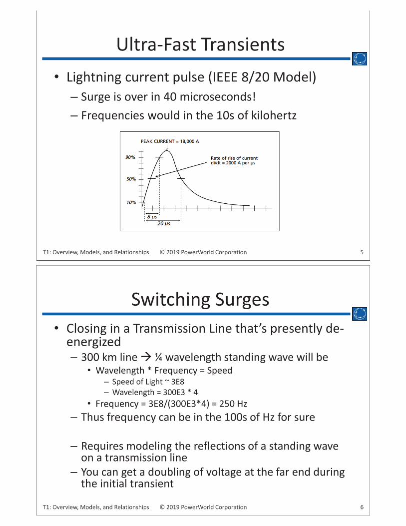
• Lightning current pulse (IEEE 8/20 Model)– Surge is over in 40 microseconds!– Frequencies would in the 10s of kilohertz
Ultra-Fast Transients
6© 2019 PowerWorld CorporationT1: Overview, Models, and Relationships
• Closing in a Transmission Line that’s presently de-energized– 300 km line ¼ wavelength standing wave will be
• Wavelength * Frequency = Speed– Speed of Light ~ 3E8– Wavelength = 300E3 * 4
• Frequency = 3E8/(300E3*4) = 250 Hz– Thus frequency can be in the 100s of Hz for sure
– Requires modeling the reflections of a standing wave on a transmission line
– You can get a doubling of voltage at the far end during the initial transient
Switching Surges

7© 2019 PowerWorld CorporationT1: Overview, Models, and Relationships
• Fast Current Transients (100 – 200 Hz).
Stator Current Transients
Krause, P.C.; Nozari, F.; Skvarenina, T.L.; Olive, D.W., "The Theory of Neglecting Stator Transients," Power Apparatus and Systems, IEEE Transactions on , vol.PAS-98, no.1, pp.141,148, Jan. 1979
8© 2019 PowerWorld CorporationT1: Overview, Models, and Relationships
• The mechanical system of the generator turbine will have mechanical resonant frequency (or frequencies)
• For large generators like big coal plants these can be on the order of 18 – 25 Hz.– Note: a generator operator needs to be cognizant of this as they
startup a generator. When the generator goes through this resonant speed it can create mechanical oscillations.
• Typically the electrical system resonant frequencies are much higher than this, so it’s not a concern
• However– Series capacitors near a generator can push electrical system
resonance lower into this range– Can lead to resonant interaction between electrical and
mechanical system damaging the mechanical shaft.
Sub-Synchronous Resonance
9© 2019 PowerWorld CorporationT1: Overview, Models, and Relationships
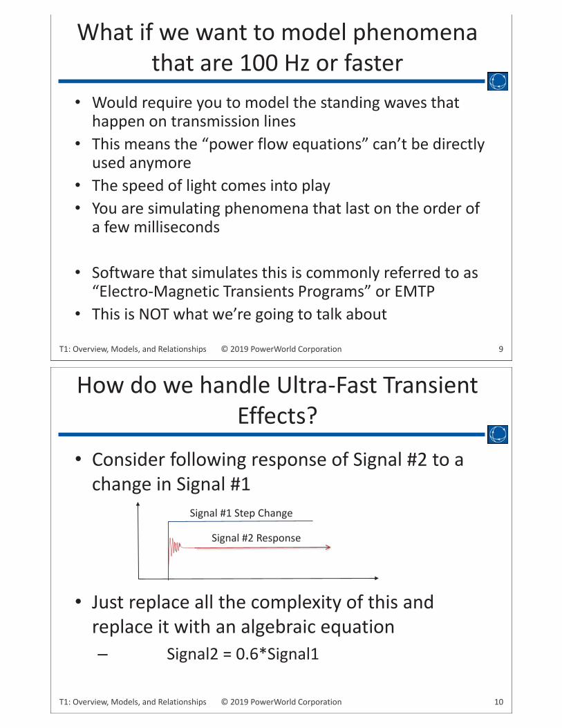
• Would require you to model the standing waves that happen on transmission lines
• This means the “power flow equations” can’t be directly used anymore
• The speed of light comes into play• You are simulating phenomena that last on the order of
a few milliseconds
• Software that simulates this is commonly referred to as “Electro-Magnetic Transients Programs” or EMTP
• This is NOT what we’re going to talk about
What if we want to model phenomena that are 100 Hz or faster
10© 2019 PowerWorld CorporationT1: Overview, Models, and Relationships
• Consider following response of Signal #2 to a change in Signal #1
• Just replace all the complexity of this and replace it with an algebraic equation– Signal2 = 0.6*Signal1
How do we handle Ultra-Fast Transient Effects?
Signal #1 Step Change
Signal #2 Response

11© 2019 PowerWorld CorporationT1: Overview, Models, and Relationships
Time Scale of Dynamic Phenomena
P. Sauer and M. Pai, Power System Dynamics and Stability, Stipes Publishing, 2006.
Lightning Propagation
Switching Surges
Stator Transients andSubsynchronous Resonance
Transient Stability
Governor and Load Frequency Control
Boiler and Long-Term Dynamics
10-7 10-5 10-3 0.1 10 103 105
Time (Seconds)
Transient Stability:10 milliseconds up to 100 seconds
12© 2019 PowerWorld CorporationT1: Overview, Models, and Relationships
• The power flow is used to determine a quasi steady-state operating condition for a power system– Goal is to solve a set of algebraic equations
• g(y) = 0 [y variables are bus voltage and angle]– Models employed reflect the steady-state
assumption, such as generator PV buses, constant power loads, LTC transformers.
Power Flow

13© 2019 PowerWorld CorporationT1: Overview, Models, and Relationships
• Contingency re-solves the power flow equations after a change (say opening a line)
• You get a new steady-state (algebraic) equation solution
• But what if system goes unstable before you get to the new system state?
Contingency Analysis
EventTime
State(Voltage)
EventTime
State(Voltage) System “blows up”
and goes unstable
Power Flow Based Contingency Analysis finds this new point
Transient Stability simulates how you get from the initial state to a new steady state
C ii
nstable be
hs
14© 2019 PowerWorld CorporationT1: Overview, Models, and Relationships
• Transient stability is used to determine whether following a contingency the power system returns to a steady-state operating point– Goal is to solve a set of differential and algebraic equations,
• dx/dt = f(x,y) [y variables are bus voltage and angle]• g(x,y) = 0 [x variables are dynamic state variables]
– Starts in steady-state, and hopefully returns to a new steady-state.
– Models reflect the transient stability time frame (up to dozens of seconds)• Slow Values Treat as constants
– Some values assumed to be slow enough to hold constant (LTC tap changing)• Ultra Fast States Treat as algebraic relationships
– Synchronous machine stator current dynamics, voltage source converter dynamics (DC transmission, portions of wind turbine models)
Power Flow vs. Transient Stability

15© 2019 PowerWorld CorporationT1: Overview, Models, and Relationships
• Commercial Software typically uses explicit integration1. Start with solved Power Flow (similar to , =
• The “Initial” or “Boundary” Conditions• Gives initial values for all the variables (Voltage, Angle)
2. Derivatives at “steady state” are zero by definition, thus use the equation = = , and solve for
3. Use numerical integration to simulate going forward in time• Many ways to do this (half of an entire class in graduate school was
dedicated to this), but let’s just consider the Forward Euler’s method because it’s simple to explain
• Important user choice is the Time Step that will be used in numerical integration
Transient Stability Solution Process
16© 2019 PowerWorld CorporationT1: Overview, Models, and Relationships
• Already have initial and • Initialize = 0 and = 0• Choose a Time Step that will be used in numerical
integration
1. Calculate new : = + ,– called the “integration time step”– Many ways to do this. This is a “Forward Euler”
2. Calculate new : Solve , =– Called solving the “network boundary equations”– Very similar to power flow equation, but use complex currents instead
3. Increment time : = +4. Increment : = + 15. Go back to 1 repeat
Transient Stability Numerical Integration

17© 2019 PowerWorld CorporationT1: Overview, Models, and Relationships
• Non-windup versus Windup Limits– Think an old “windup” clock with a spring. Eventually, the
spring reaches a point where it can no longer “windup” anymore
– A “non-windup” limit must be enforced between step 1 and 2 so that the state never goes past its limit
Other Tricks in Integration
1 +1 +in
Max
Min1 +1 + Max
Min
Mi1111
Mi
Max
18© 2019 PowerWorld CorporationT1: Overview, Models, and Relationships
Sub-Interval Integration
One Time Step ( t)
t + ttx3 x3
x2 x1
x3x2
x1
x3x2
x0
1 2 3 87654
• Chop-up the time step into pieces so that you can use a smaller time step only for states that require this.
Subinterval updates updates updates updates1 = + 8 , Assume constant Assume constant Assume constant
2 = + 8 , = + 4 , Assume constant Assume constant
3 = + 8 , Assume constant Assume constant Assume constant
4 = + 8 , = + 4 , = + 2 , Assume constant
5 = + 8 , Assume constant Assume constant Assume constant
6 = + 8 , = + 4 , Assume constant Assume constant
7 = + 8 , Assume constant Assume constant Assume constant
8 = + 8 , = + 4 , = + 2 , = + 1 ,

19© 2019 PowerWorld CorporationT1: Overview, Models, and Relationships
Physical Structure Power System Components
Generator
P, Q
Network
Network control
Loads
Load control
Fuel Source
Supply control
Furnace and Boiler
Pressure control
Turbine
Speed control
V, ITorqueSteamFuel
Electrical SystemMechanical System Elm
Fa T G N L
Voltage Control
P. Sauer and M. Pai, Power System Dynamics and Stability, Stipes Publishing, 2006.
20© 2019 PowerWorld CorporationT1: Overview, Models, and Relationships
Machine
Governor
Exciter
LoadChar.
Load Relay
LineRelay
Stabilizer
Transient Stability Models in the Physical Structure
Generator
P, Q
Network
Network control
Loads
Load control
Fuel Source
Supply control
Furnace and Boiler
Pressure control
Turbine
Speed control
V, ITorqueSteamFuel
Electrical SystemMechanical System Elm
Fa T G N L
Voltage Control
P. Sauer and M. Pai, Power System Dynamics and Stability, Stipes Publishing, 2006.

21© 2019 PowerWorld CorporationT1: Overview, Models, and Relationships
• The most comprehensive book on this type of analysis is the by Prabha Kundur and is called Power System Stability and Control published in 1994
• Book is too detailed for a classroom textbook, but it is a really great as a reference book once you’re working
Transient Stability Modeling
22© 2019 PowerWorld CorporationT1: Overview, Models, and Relationships
• Basics of Synchronous Machine Model– Exciter applies DC current to rotor making it an electromagnet – Turbine/Governor spins rotor– Spinning magnet creates AC power
Synchronous Machine
ExciterCreates a DC voltage to apply to Rotor Winding, resulting in an electromagnet
Turbine/ GovernorCreates a mechanical torque to spin the rotor
Machine

23© 2019 PowerWorld CorporationT1: Overview, Models, and Relationships
• Start with Newton’s second law– Force = Mass * Acceleration
– = and =• We have a rotational system though, so instead
we end up with something a little different– Torque = Moment of Inertia * Angular Acceleration
– = and =
Mechanical Modeling a Generator
24© 2019 PowerWorld CorporationT1: Overview, Models, and Relationships
• You were introduced to per unit systems for the power flow• This concept is everywhere in transient stability analysis• It can be VERY confusing to everyone, but is a vital part of
how these software tools are written and how data is provided by manufacturers
• You need to be very careful when entering data into any software package to make sure you’re handling per unit correctly– = synchronous speed
• = 2 = 2 3.14159 60 = 376.99– H = Inertia Constant– Torque Base = MVABase/– = treated as per unit speed deviation =
Per Unit Systems (again and always)

25© 2019 PowerWorld CorporationT1: Overview, Models, and Relationships
• Anyway, after a lot of additional algebra, software tools model the swing equations as follows with values in per unit– = and =
• If you use a more complete model of the rotor of a generator, then the term has some inherent damping in it
• In academic settings, as we’ll introduce in a moment, the rotor modeling has no inherent damping in it (which makes your results really oscillate)– To overcome this, folks often add an extra term as follows
– This term should NOT be used to model the damping in the more accurate rotor models such as GENROU, GENSAL, GENTPF, GENTPJ, etc.
Generator Swing Equation
= 1 +
26© 2019 PowerWorld CorporationT1: Overview, Models, and Relationships
• This can be a few weeks worth of lectures in a graduate level course– We’re going to take 4 slides, so don’t worry about the details here
• Physical Structure Terms– Positional Winding Terms
• Stator (Stationary portion of generator)• Rotor (Rotating portion of generator)
– Functional Winding Terms• Armature Winding (three-phase AC winding that carries the power)
– Normally this is on the Stator• Field Winding (DC current winding)
– Normally this is on the Rotor• Amortisseur Winding (or damper winding)
– An extra winding that provides start-up torque and damping– Basically a winding that causes a force that attempts to bring machine to synchronous speed (60
Hz)• Armature Poles
– Following slide shows two dots for each (A, B, C) phase one “in” and one “out”– This represents a 2 pole machine– If you just repeated this 4 additional times for each phase then you’d have an “8 pole” machine– More poles means the machine doesn’t need to spin as fast to create 60 Hz
Modeling the Generator Rotor

27© 2019 PowerWorld CorporationT1: Overview, Models, and Relationships
• d = Direct Axis– Spinning axis directly in line with the “North Pole” of
the field winding• q = Quadrature Axis
– Spinning axis 90 degrees out of phase with thedirect axis
• Rotor Angle ( )– Angle between
Direct axis andPhase A axis
Modeling the Generator Rotor
Page 46 of Kundar BookRight-Hand rule defines axes of phase a, b, and c as well as direct axis
28© 2019 PowerWorld CorporationT1: Overview, Models, and Relationships
• Algebra and trigonometry end up being extremely complex– Results give inductances between phases that are a
function of the cosine of rotor angle– A simplification is done to transform the abc phase
quantities into another reference frame• Called the dq0 transformation • Might hear “Park’s
Transformation” after Robert H. Park who did something very similar in 1929
Deriving Equations for Rotor

29© 2019 PowerWorld CorporationT1: Overview, Models, and Relationships
• This is a very similar idea as symmetrical components when discussing fault analysis (different matrix conversion though)
• We can say thanks to engineers who figured this all out for us 80 years ago!• We end up with 14 equations that go through conversion similar to following• Also do some more “magic” per unit assignment to make things clean-up more
dq0 Transformation
dq0
30© 2019 PowerWorld CorporationT1: Overview, Models, and Relationships
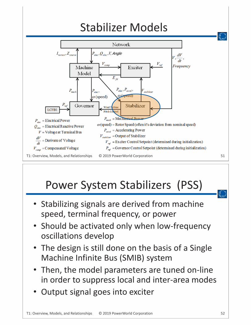
• Generators can have several classes of models assigned to them– Machine Models– Exciter– Governors– Stabilizers
• Others also available – Excitation limiters, voltage compensation, turbine load
controllers, and generator relay model
Generator Models

31© 2019 PowerWorld CorporationT1: Overview, Models, and Relationships
Generator Models
32© 2019 PowerWorld CorporationT1: Overview, Models, and Relationships
Machine Models

33© 2019 PowerWorld CorporationT1: Overview, Models, and Relationships
• The Classical Model (GENCLS)- very simplified • Represents the machine dynamics as a fixed voltage
magnitude behind a transient impedance Ra + jXd’.
• Only 2 states equationsfor and
• Used in academic settings because of its simplicity but is not recommended for actual power system studies
Machine Models
+-or
== 1 1 +
34© 2019 PowerWorld CorporationT1: Overview, Models, and Relationships
• PowerWorld Simulator has many more realistic models that can be easily used– Many books and papers discuss the details
• Salient pole – GENSAL machine model • Round rotor – GENROU model• Generator with Transient Saliency – GENTPF
and GENTPJ models– These models are becoming required in WECC
(Western US and Canada)
More Realistic Models

35© 2019 PowerWorld CorporationT1: Overview, Models, and Relationships
The GENROU modelprovides a very good approximation for thebehavior of a synchronousgenerator over the dynamicsof interest during a transient stability study (up to about 10 Hz).It is used to represent a solid rotor machine withthree damper windings.
More than 2/3 of the machines in the 2006 NorthAmerican Eastern Interconnect case (MMWG) are
represented by GENROU models.
GENROU Model
The “d” and “q” values here are referring back to the Direct and Quadrature discussion from earlier
36© 2019 PowerWorld CorporationT1: Overview, Models, and Relationships
Exciter Models

37© 2019 PowerWorld CorporationT1: Overview, Models, and Relationships
• Three distinctive types– Type DC excitation systems
• Direct current generator with a commutator as source of excitation system power
• Original exciters (1920s- 1960s)– Type AC excitation systems
• Usually means you place a synchronous motor on the same shaft as the generator
• Use the AC voltage created by this motor to feed a rectifier and feed back to the DC voltage to the generator field
– Type Static (ST) excitation systems• Similar to AC, except power is supplied through transformers or
auxiliary generator windings and rectifiers• Source might be the output of generator itself, or an auxiliary feed
from somewhere else
Types of Exciters
38© 2019 PowerWorld CorporationT1: Overview, Models, and Relationships
• Models must be suitable for modeling severe disturbances as well as large perturbations
• Generally, these are reduced order models that do not represent all of the control loops– For example, there may be an entire control system
ensuring that a particular variable doesn’t exceed a limit– This control system is replaced by an algebraic equation that
says (Vr < Vrmax)– Again, Fast Variable Algebraic Equations
• These models do not generally represent delayed protective and control functions that may come into play in long-term dynamic performance studies
Excitation System Models
IEEE Standard 421.5, IEEE Recommended Practice for Excitation System Models for Power System Stability Studies, Aug. 1992

39© 2019 PowerWorld CorporationT1: Overview, Models, and Relationships
• Excitation subsystems for synchronous machines may include voltage transducer and load compensator, excitation control elements, exciter, and a power system stabilizer
Excitation System Models
Measurementand
Compensation
Machineand
Network Equations
ExciterExcitation control
elements
VT IT
VSI
VC
IFDVFD
VR
VS
VREF
VOELVUEL
Stabilizer
40© 2019 PowerWorld CorporationT1: Overview, Models, and Relationships
• VREF is the voltage regulator reference signal– Is calculated to satisfy the initial operating conditions.– In Simulator this will be called the Exciter Setpoint (Vref)– This represents the “knob” that the generator operator
turns to move the voltage higher or lower• Efd is the field voltage
– Adjusting the DC field voltage changes the DC field current and thus impacts the terminal AC voltage of generator
– If Efd were a constant, the machine would not have voltage control.
– The exciter systematically adjusts Efd in attempt to maintain the terminal voltage equal to the reference signal.
• Ifd is the field current
Exciter Models in General

41© 2019 PowerWorld CorporationT1: Overview, Models, and Relationships
• Ec is the “compensated voltage”– Typically this is just the generator terminal voltage– Could regulate a point some impedance away (such
as half way through the step-up transformer)• Ec = Vt – Xcomp*It
• Typical optional feedback signals– Vs is from the stabilizer– VUEL is from an under excitation limiter– VOEL is from an over excitation limiter
Comments on Typical Exciter
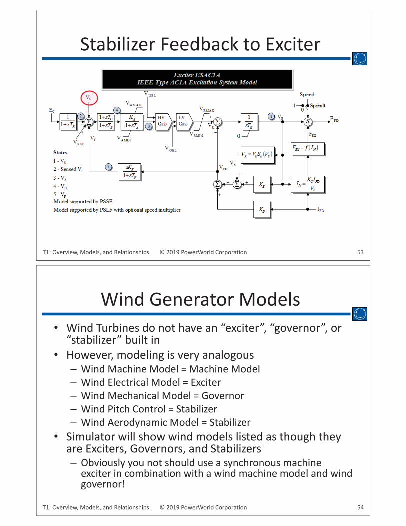
42© 2019 PowerWorld CorporationT1: Overview, Models, and Relationships
Typical Exciter Block Diagram
Rectifier
Laplace Transforms! s = Laplace Operator

43© 2019 PowerWorld CorporationT1: Overview, Models, and Relationships
• Derivative Block Output (VF)– Output at steady state is zero (definition of “steady” state)
• Stabilizer Signal (VS)– Output at steady state is also
zero (again by definition)• Delay Block for signal (EC)
– Represents measurement delay• Assume you know (VR)
– (VUEL) and (VOEL) are zero at steady state– State 4 is then VR/KA– Output summation is same as state 4 (treat “s” as zero at steady state)
• Calculation of VREF– VREF = EC +VR/KA
Example “Back-Solving”for Initial States
Output of Delay Block
Input
Output of Lead/Lag
input
44© 2019 PowerWorld CorporationT1: Overview, Models, and Relationships
Governor Models

45© 2019 PowerWorld CorporationT1: Overview, Models, and Relationships
• Steady-state speed of a synchronous machine determined by the speed of the prime mover that drives its shaft
• Prime mover thus provides a mechanism for controlling the synchronous speed – Diesel engines– Gasoline engines– Steam turbines– Hydroturbines
• Prime mover output affects the mechanical torque to the shaft (TM)
Prime Movers and Turbine Models
46© 2019 PowerWorld CorporationT1: Overview, Models, and Relationships
• A governor senses the speed (or load) of a prime mover and controls the fuel (or steam) to the prime mover to maintain its speed (or load) at a desired level
• Essentially, a governor ends up controlling the energy source to a prime mover so that it can be used for a specific purpose
• Consider driving a car you act as a governor to control the speed under varying driving conditions
What is a Governor?
Woodward, “Governing Fundamentals and Power Management,” Technical Manual 26260, 2004. [Online]. Available: http://www.woodward.com/pubs/pubpage.cfm
47© 2019 PowerWorld CorporationT1: Overview, Models, and Relationships
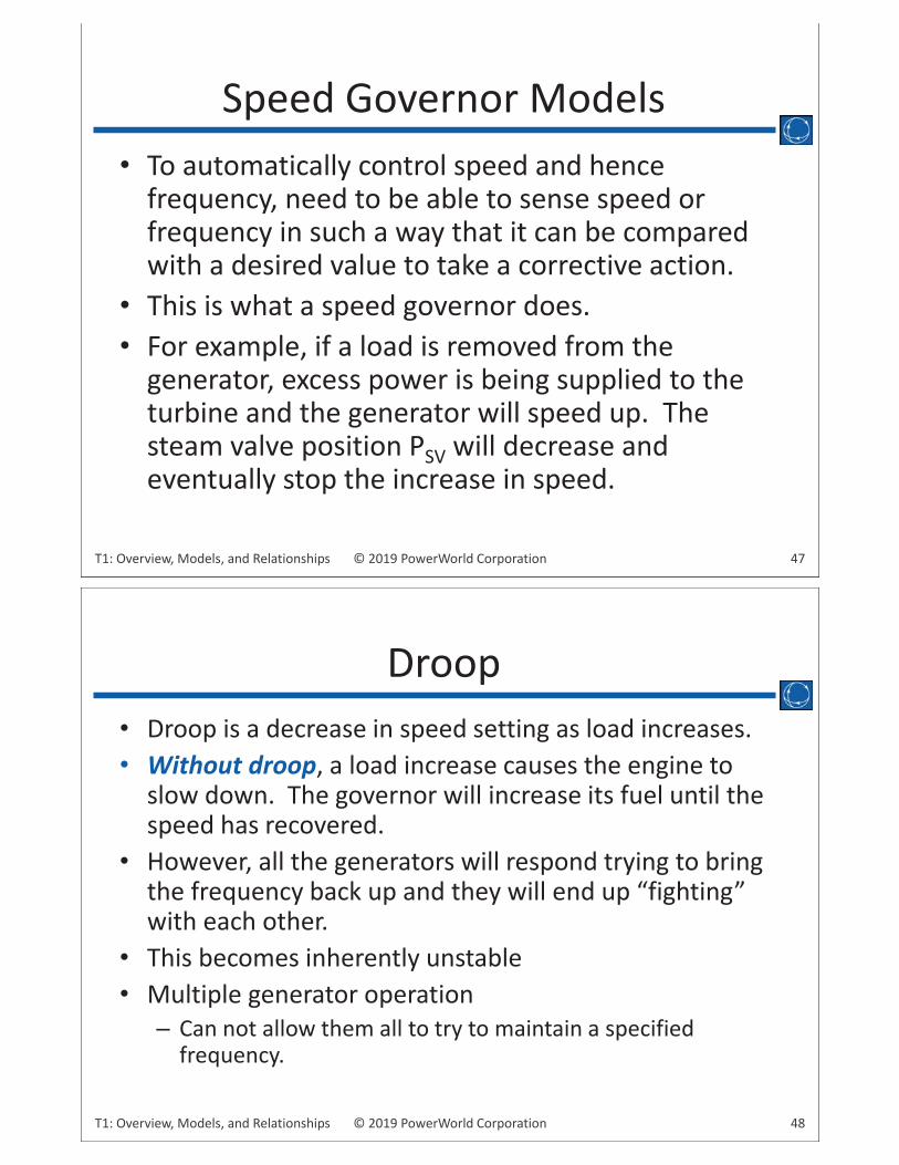
• To automatically control speed and hence frequency, need to be able to sense speed or frequency in such a way that it can be compared with a desired value to take a corrective action.
• This is what a speed governor does.• For example, if a load is removed from the
generator, excess power is being supplied to the turbine and the generator will speed up. The steam valve position PSV will decrease and eventually stop the increase in speed.
Speed Governor Models
48© 2019 PowerWorld CorporationT1: Overview, Models, and Relationships
• Droop is a decrease in speed setting as load increases.• Without droop, a load increase causes the engine to
slow down. The governor will increase its fuel until the speed has recovered.
• However, all the generators will respond trying to bring the frequency back up and they will end up “fighting” with each other.
• This becomes inherently unstable• Multiple generator operation
– Can not allow them all to try to maintain a specified frequency.
Droop
49© 2019 PowerWorld CorporationT1: Overview, Models, and Relationships
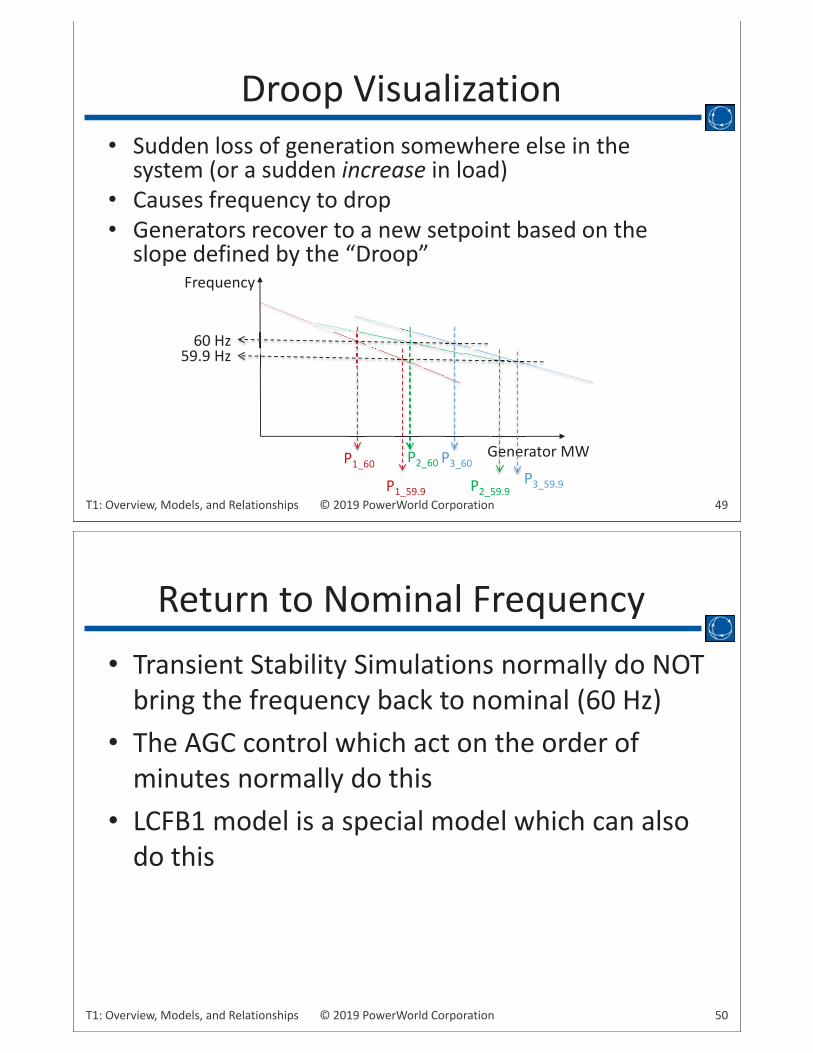
• Sudden loss of generation somewhere else in the system (or a sudden increase in load)
• Causes frequency to drop• Generators recover to a new setpoint based on the
slope defined by the “Droop”
Droop Visualization
Frequency
Generator MW
60 Hz
P1_60 P2_60 P3_60
59.9 Hz
PP Gennern
P1_59.9 P2_59.9P3_59.9
50© 2019 PowerWorld CorporationT1: Overview, Models, and Relationships
• Transient Stability Simulations normally do NOT bring the frequency back to nominal (60 Hz)
• The AGC control which act on the order of minutes normally do this
• LCFB1 model is a special model which can also do this
Return to Nominal Frequency
51© 2019 PowerWorld CorporationT1: Overview, Models, and Relationships
Stabilizer Models
52© 2019 PowerWorld CorporationT1: Overview, Models, and Relationships
• Stabilizing signals are derived from machine speed, terminal frequency, or power
• Should be activated only when low-frequency oscillations develop
• The design is still done on the basis of a Single Machine Infinite Bus (SMIB) system
• Then, the model parameters are tuned on-line in order to suppress local and inter-area modes
• Output signal goes into exciter
Power System Stabilizers (PSS)
53© 2019 PowerWorld CorporationT1: Overview, Models, and Relationships
Stabilizer Feedback to Exciter
54© 2019 PowerWorld CorporationT1: Overview, Models, and Relationships
• Wind Turbines do not have an “exciter”, “governor”, or “stabilizer” built in
• However, modeling is very analogous– Wind Machine Model = Machine Model– Wind Electrical Model = Exciter– Wind Mechanical Model = Governor– Wind Pitch Control = Stabilizer– Wind Aerodynamic Model = Stabilizer
• Simulator will show wind models listed as though they are Exciters, Governors, and Stabilizers– Obviously you not should use a synchronous machine
exciter in combination with a wind machine model and wind governor!
Wind Generator Models

55© 2019 PowerWorld CorporationT1: Overview, Models, and Relationships
• Load fall into two categories in a transient stability– Static Load Model
• Normally a function of voltage and/or frequency
• Discharge Lighting (Fluorescent Lights)– Voltage Dependent.
– Dynamic Load Models• Induction Motors
• Load Characteristic Models end up being combinations of all these– “Complex” load models include all of them in various
proportions
Load Characteristic Models
31 2
5 64
1 2 3 7
4 5 6 8
1
1
nn nload
n nnload
P P a v a v a v a f
Q Q a v a v a v a f
56© 2019 PowerWorld CorporationT1: Overview, Models, and Relationships
Load Characteristic Models: CMPLDW• CMPLDW Load Characteristic Models end up being
combinations of all these models in the following manner:

57© 2019 PowerWorld CorporationT1: Overview, Models, and Relationships
Load Characteristic Models: CMPLDW• Data management issue
– Up to 130 parameters– Number of parameters can differ depending on the
type of motor used– Pushing the limits of how much data can be reasonably
managed• Group together models with the same parameters• Create new objects in Simulator
– Load Model Groups– Load Distribution Equivalent Types– More details on these new object in next training
section
58© 2019 PowerWorld CorporationT1: Overview, Models, and Relationships
• Basic idea:
Load Characteristic Models: CMPLDW
Low Side Bus Rfdr, Xfdr
Load Bus
LTC Tfixhs s Tfixls
Bss
Bf1 Bf2
Tdel Tdelstep Rcmp Xcmp MVABase
Xxf
Transmission System Bus
Transmission System Bus
LTC TdelTransformer Control former Csf
Tmax Step Vmin Vmax
Pinit + jQinit
XxPinit + jQinit
Pnew + jQnew
Fb
Bf1 = ( Fb )(Bf1+Bf2) Bf2 = (1-Fb)(Bf1+Bf2)
The internal model used by the transient stability numerical simulation structurally does the following.
1. Creates two buses called Low Side Bus and Load Bus 2. Creates a transformer between Transmission Bus and Low
Side Bus 3. Creates a capacitor at the Low Side Bus 4. Creates a branch between Low Side Bus and Load Bus 5. Moves the Load from the Transmission Bus to the Load Bus
PLS + jQLS LS
Tap

Blank Page
Blank Page