transient conduction lumped thermal capacitance method analytical method: separation of variables...
TRANSCRIPT

TRANSIENT CONDUCTION
• Lumped Thermal Capacitance
Method
• Analytical Method: Separation of Variables
• Semi-Infinite Solid: Similarity Solution
• Numerical Method: Finite Difference Method

Lumped Thermal Capacitance Methodnegligible spatial
effect( , , , ) ( )T x y z t T t
,h T
in g out stE E E E st out 0E E
out ( ) ,sE hA T t T st
dTE Vc
dt
( ) 0s
dTVc hA T t T
dt
volume Vsurface area As
,c
(0) iT T( )T t

excess temperature:
( ) ( )t T t T
( ) 0s
dTVc hA T t T
dt
0,shAd
dt Vc
( ) exp shAt C t
Vc
initial condition:
(0) (0) i iT T T T
(0) i C
( ) ( )
i i
t T t T
T T
exp shA
tVc

thermal time constant
1t
shAVc
: convection resistance
ttR C
1t
s
RhA
tC Vc : lumped thermal capacitance
Thermocouple?
( )exp s
i
hAtt
Vc

Transient temperature response of lumped capacitance solids for different thermal time constant t

Seebeck effect and Peltier effect
2
1
( ) ( )T
B ATV S T S T dT
2 1B AS S T T A B
T2
T1
V
+
-
Seebeck effect (1821)
AB
↑I
B A ABQ I I
Peltier effect (1834)
T2
T1
volume Vsurface area As
( )T t,h T
,c
(0) iT T
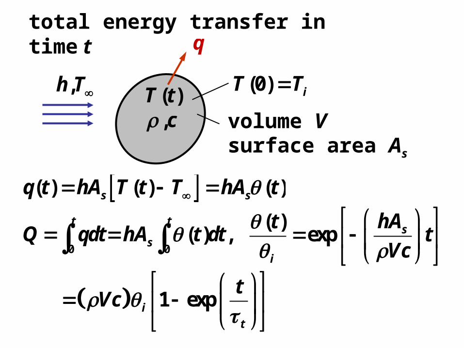
total energy transfer in time t q
0
t
Q qdt
( ) ( ) ( )s sq t hA T t T hA t
0( ) ,
t
shA t dt
1 expi
t
tVc
( )exp s
i
hAtt
Vc
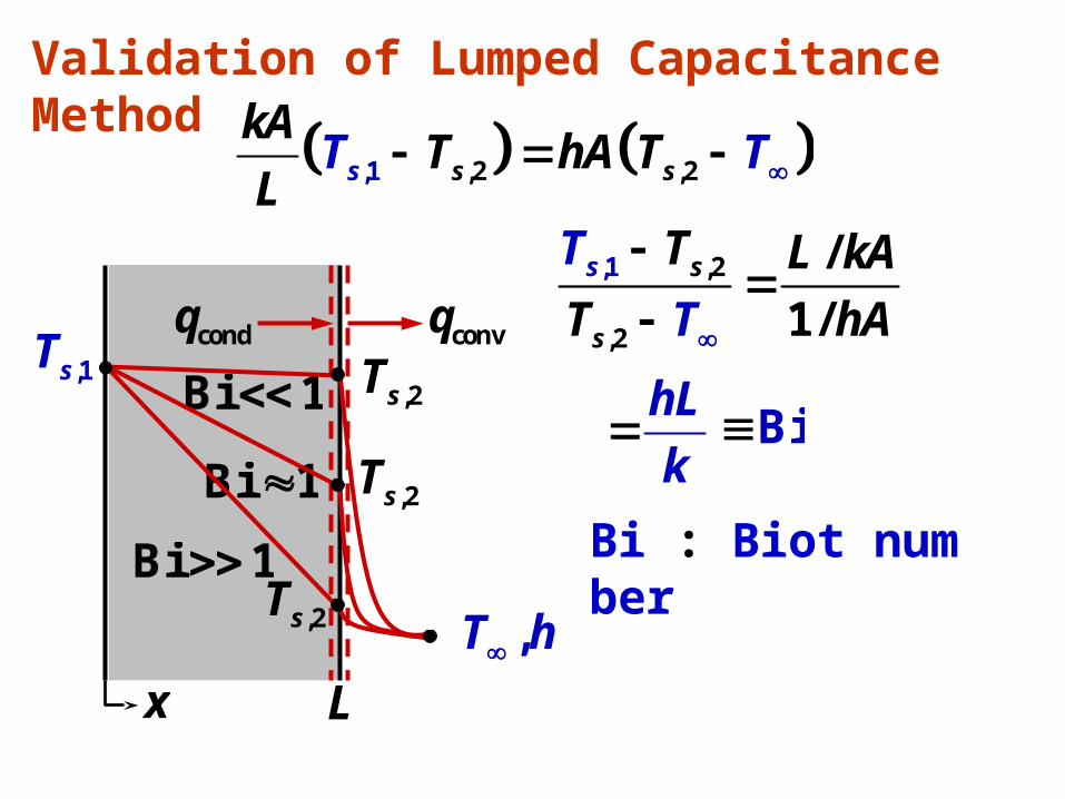
Validation of Lumped Capacitance Method ,21 ,2, ss s
kAT hA T
LT T
,2
,2
,1 /
1/s
s
sT
T
T L kA
T hA
hL
k Bi
Bi : Biot number
x L
,1sT
,T h
,2sT
Bi 1
Bi 1
Bi 1
condq convq
,2sT
,2sT

Transient temperature distributions for different Biot numbers in a plane wall symmetrically cooled by convection

When
spatial effect is negligible.i 0 ,B .1chL
k
Lc : characteristic length c
s
VL
A
( )exp s
i
hAtt
Vc
s
c
hA t ht
Vc cL
2c
c
hL kt
k cL
2c
chL
k
t
L
FBi o
( )exp Bi Fo
i
t
Fo : Fourier number (dimensionless time)

Find: Total time tt required for the two-step process
Assumption: Thermal resistance of epoxy is negligible.
Example 5.3
sA
2
,
=40 W/m K=175 C
o
o
hT
sur , 175 CoT
Step 1: Heating(0 )ct t
2
,
=10 W/m K=25 C
c
c
hT
sur , 25 CcT
Step 2: Cooling( )e tt tt
t = 0
Ti,o = 25°C
t = tc t = te t = tt300 s
Tc = 150°C Te = ?°C Tt = 37°C
heating
coolingcuring
aluminum T(0) = Ti,o = 25°C T(tt) = 37°C
epoxy = 0.8
2L = 3 mm

,h T
Epoxy
sA
2 L surT
Biot numbers for the heating and cooling processes
4Bi 3.4 10 ,oh
h L
k 5Bi 8.5 10c
c
h L
k
3177 W/m K, 875 J/kg K, 2770 kg/mk c Aluminum:
Thus, lumped capacitance approximation
can be applied.
2 s
dTc LA
dt
4 4sur( ) ( )
cLdTdt
h T T t T T t
qconv
qrad
2 ( )sh A T t T 4 4sur2 ( )sA T t T
T(t)
st in out gE E E E

Heating process
Curing process
Cooling process
tc = 124 s
Te = 175°C
tt = 989 s
t = 0
Ti,o = 25°C
t = tc t = te t = tt300 s
Tc = 150°C Te = ?°C Tt = 37°C
heating
coolingcuring
Numerical solutions
,4 40
, sur,( ) ( )
c
i o
cT
To o o
cLdTdt
h T T t T T t
t
4 4sur( ) ( )
cLdTdt
h T T t T T t
4 4, sur,( ) ( )
e
c c
et
t To o o
T cLdTdt
h T T t T T t
4 4, sur,( ) ( )
t
e e
t T
t Tc c c
t cLdTdt
h T T t T T t

Total time for the two-step process :
989 stt
Intermediate times : 124 sct 424 set

Plane wall with convection
Separation of Variables
L Lx
i.c.
b.c.
Analytical Method
,T h ,T h
2
2
T T
t x
( ,0) iT x T
0
0x
T
x
( , )x L
Tk h T L t T
x
( , , , , , , , )iT T x t T k L h T
( , )T x t
( ,0)
i
T x
T

Dimensional analysis
dimensionless variables
Fo: Fourier number, Bi: Biot number
L: m [L]
( , , , , , , , )iT T x t T k L h T
, , : K [ ],iT T T D : m [ ],x L : s [ ]t T2 2 1: m /s [ ],L T
3 -3 1: W/m K kg m/s K [ ]k LMT D 2 3 -3 1: W/m K kg/s K [ ]h MT D
* ,i
T T
T T
* ,
xx
L *
2F ,o
tt
L
Bi
hL
k
* * * *( , ;Bi)x t
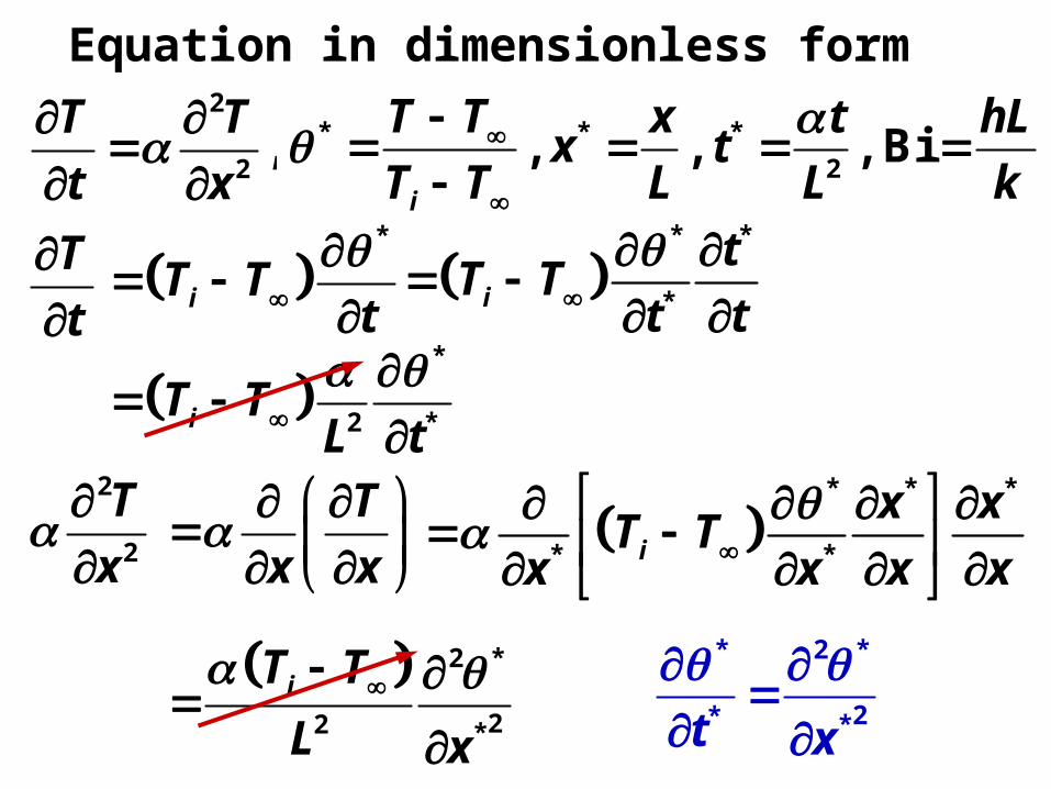
Equation in dimensionless form2
2,
T T
t x
* * *
2, , , Bi
i
T T x t hLx t
T T L L k
T
t
*
iT Tt
* *
*i
tT T
t t
*
2 *iT TL t
2
2
T
x
T
x x
* * *
* *i
x xT T
x x x x
2 *
22 *
iT T
L x
* 2 *
2* *t x

initial condition boundary conditions
* * *
2, , , Bi
i
T T x t hLx t
T T L L k
( ,0) iT x T * *( ,0) 1x
0x
T
x
*
*
*
0
0i
x
T T
L x
*
*
*
0
0x
x
( , )x L
Tk h T L t T
x
*
*
*
1
i
x
k T T
L x
* *(1, )ih T T t
*
** *
*
1
Bi (1, ) 0x
tx

Drop out * for convenience afterwards
2
2t x
0 1
, ,( ,0) 1 0 Bi (1, ) 0x x
x tx x
( , ) ( ) ( )x t X x t
,X X X
X
2
2 0,X X 2 0

boundary conditions
0
(0) ( ) 0x
X tx
(0) 0X
1
Bi (1, )x
tx
(1) ( )X t Bi (1) ( )X t
(1) Bi (1) ( ) 0X X t (1) Bi (1) 0X X
0 1
0, Bi (1, ) 0x x
tx x

b.c.
( ) :X x 2 0X X (0) 0,X (1) Bi (1) 0X X
1 2( ) sin( ) cos( )X x C x C x
1 2( ) cos( ) sin( )X x C x C x
1(0) 0X C
2 2(1) Bi (1) sin Bi cosX X C C
2 Bicos sin 0C tan Bi
( ) cos( )n n nX x a x
tan Bi,n n n such that 1,2,3,n

initial condition
( ) :t 2 0 2( ) exp( )n n nt b t
2
1
( , ) exp( )cos( )n n nn
x t c t x
( ) cos( )n n nX x a x
1
( ,0) 1 cos( )n nn
x c x
1
01
2
0
cos( )
cos ( )
n
n
n
x dxc
x dx
4sin
2 sin(2 )n
n n

Approximate solution
at x = 0, Bi = 1.0Fo = 0.1 Fo = 1
1 1.0393 0.53392 -0.0469 -1.22 10-5
3 0.0007 4.7 10-20
2
1
( , ) exp( )cos( )n n nn
x t c t x
2
1 1 1( , ) exp( )cos( )x t c t x 2
2 2 2exp( )cos( )c t x
1 2
When
,Fo 0.2t 2
2 2 22
1 1 1
exp( )cos( )1
exp( )cos( )
c t x
c t x

See Table 5.1
21 1 1( , ) exp( )cos( )x t c t x
Approximate solution
When
Fo 0.2,t
21 1(0, ) exp( )t c t 0
1
0
( , )cos( )
x tx
tan Bin n

10
( , )cos( )
x tx
20 1 1exp( )c t

( , ) ic T x t T dV ( , ) iT x t dVTc
total energy transfer (net out-going)
maximum amount of energy transfer
( , ) iT x t T( )Q t
0 iQ cV T T
0
Q
Q
i
i
c T TdV
cV T T
1 i
i
T T T TdV
V T T
11 dV
V
1
0 10
1 cos( )x dx 1
0
1
sin1

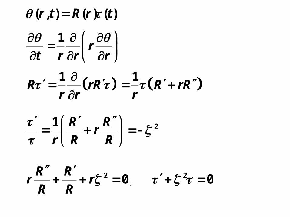
Radial systems with convection
i.c.
b.c.
rT T
rt r r r
,T h
( ,0) iT r T
0
0r
T
r
( , )o
or r
Tk h T r t T
r
or
(0, )T t finite
ro
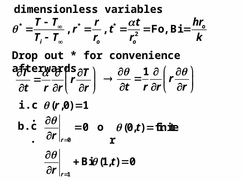
dimensionless variables
T Tr
t r r r
* * *2
, , Fo, Bi o
i o o
hrT T r tr t
T T r r k
Drop out * for convenience afterwards 1
rt r r r
i.c.
b.c.
( ,0) 1r
0
0rr
o
r(0, )t finite
1
Bi (1, ) 0r
tr
( , ) ( ) ( )r t R r t
1r
t r r r
R 1rR
r r
1R rR
r
1 R Rr
r R R
2
2 0,R R
r rR R
2 0
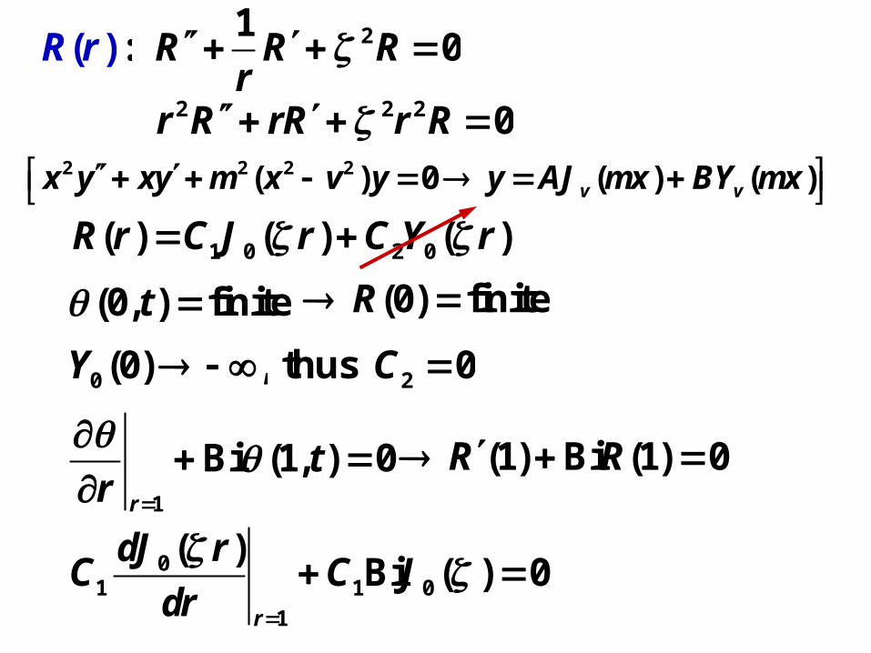
( ) :R r 210R R R
r
2 2 2 0r R rR r R
(0, )t finite (0)R finite1 0 2 0( ) ( ) ( )R r C J r C Y r
0 (0)Y , 2 0C thus
1
Bi (1, ) 0r
tr
(1) Bi (1) 0R R
01 1 0
1
( )Bi ( ) 0
r
dJ rC C J
dr
2 2 2 2( ) 0 ( ) ( )v vx y xy m x v y y AJ mx BY mx

1 1
2( ) ( ) ( )n n n
nJ x J x J x
x
0 1 1( ) ( ) ( )d
J x J x J xdx
Since
1( ) ( ) n nn n
dx J x x J x
dx
00
1
( )Bi ( ) 0
r
dJ rJ
dr
00
1
( )Bi ( )
r
dJ rJ
dr
1 0( ) Bi ( ) 0J J
0( ) ( ), n n nR r a J r 1
0
( ) Bi
( )n
n n
n
J
J
such that
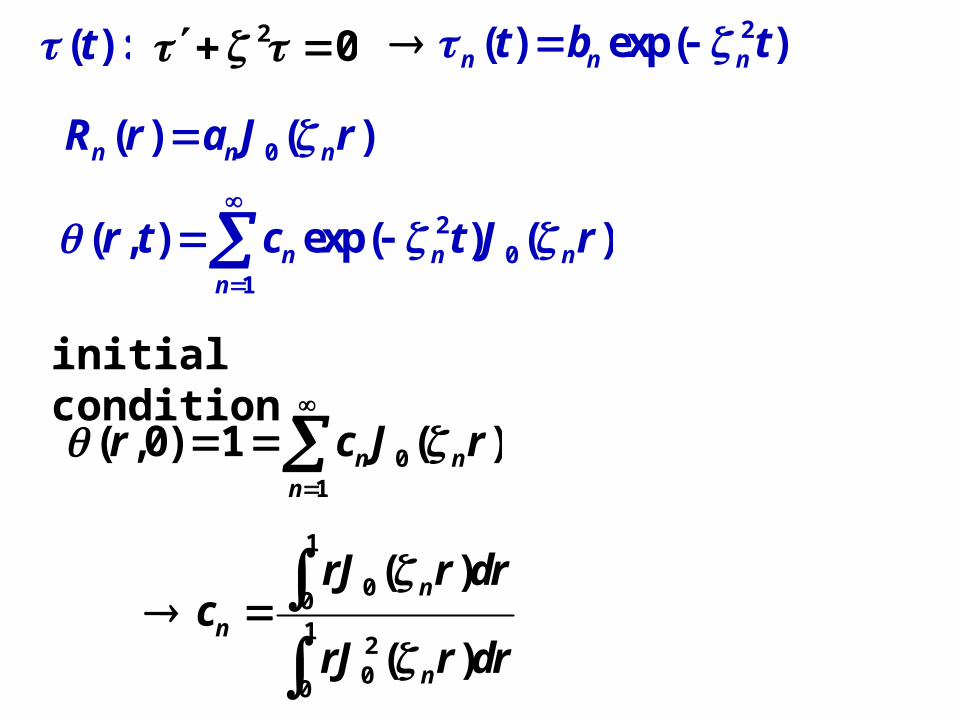
initial condition
( ) :t 2 0 2( ) exp( )n n nt b t
20
1
( , ) exp( ) ( )n n nn
r t c t J r
01
( ,0) 1 ( )n nn
r c J r
1
001
20
0
( )
( )
n
n
n
rJ r drc
rJ r dr
0( ) ( )n n nR r a J r

Approximate solution
Total energy transfer (net out-going)
Since V = L, dV = 2rdrL
21 1 0 1( , ) exp( ) ( )r t c t J r
2 21 1 0 1 1 0(0, ) exp( ) (0) exp( )t c t J c t
0 1
0
( , )( )
x tJ x
( ) ( , ) iQ t c T x t T dV , 0 iQ cV T T
1
0 0 10
0
1 11 1 ( )
QdV J r dV
Q V V
1
0 0 10
0
2 1 ( )Q
J r rdrQ
1 10
1
2 ( )1
J
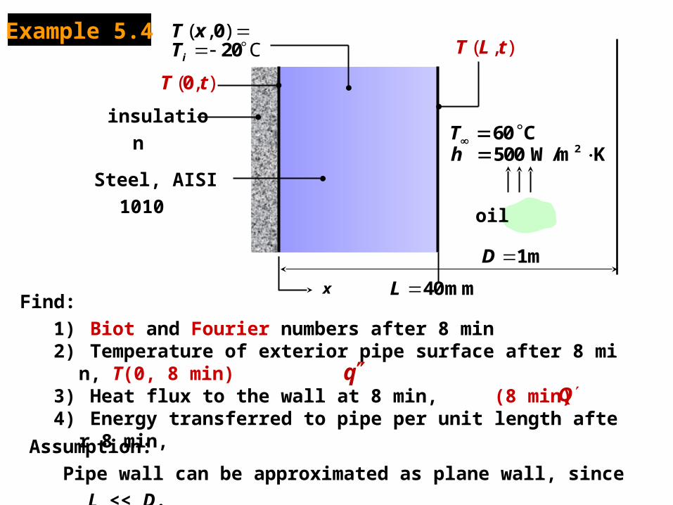
Assumption:Pipe wall can be approximated as plane wall, since L
<< D.
Example 5.4
x 40mmL
260 C500 W/m K
Th
oil
( , )C
020i
T xT
1mD
insulation
Steel, AISI 1010
( , )T L t
( , )0T t
Find: 1) Biot and Fourier numbers after 8 min2) Temperature of exterior pipe surface after 8 min, T(0, 8 min)3) Heat flux to the wall at 8 min, (8 min)4) Energy transferred to pipe per unit length after 8 min, Q
q

260 C500 W/m K
Th
oil
( , )C
020i
T xT
( , )T L t
( , )0T t
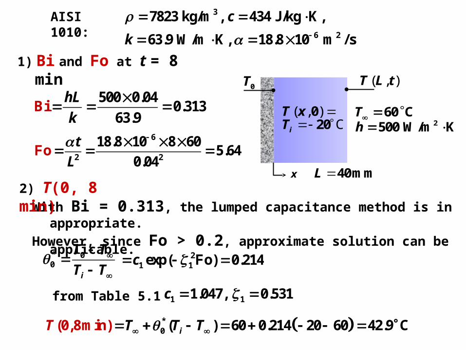
1) Bi and Fo at t = 8 min
500 0.040.313
63.9Bi
hL
k
6
2 2F
18.8 10 8 605.64
0.04o
t
L
With Bi = 0.313, the lumped capacitance method is inappropriate.However, since Fo > 0.2, approximate solution can be applicable.
* 00
i
T T
T T
2) T(0, 8 min)
21 1exp( Fo)c 0.214
*0 ( ) 60(0,8m 0.214 20 60 42.9in C) iT TT T
AISI 1010: 3
6 2
7823 kg/m , 434 J/kg K,
63.9 W/m K, 18.8 10 m / s
c
k
x
0T ( , )T L t
( , )C
020i
T xT
40mmL
260 C
500 W/m KTh
from Table 5.1 1 11.047, 0.531c

(40 ( m48 m,0 s) 480 s)h Tq T
4) The energy transfer to the pipe wall over the 8-min interval
*10
0 1
sin( )1
Q
Q
3)
0.80
0.80 ic TQ V T
*0 1( , ) cos( )iT L t T T T
2500 45.2 60 7400 W/mq
0.80 ic DL T TQ 72.73 10 J/m
x
0T ( , )T L t
( , )C
020i
T xT
40mmL
2
60 C
500 W/m K
Th
* * * * * *0 1
( , )( , ) ( )cos( )
i
T x t Tx t t x
T T
(40 mm,480 s) 60 ( 20 60) 0.214 cos(0.531) 45.2T
(480 s)q
sin(0.531)1 0.214
0.531
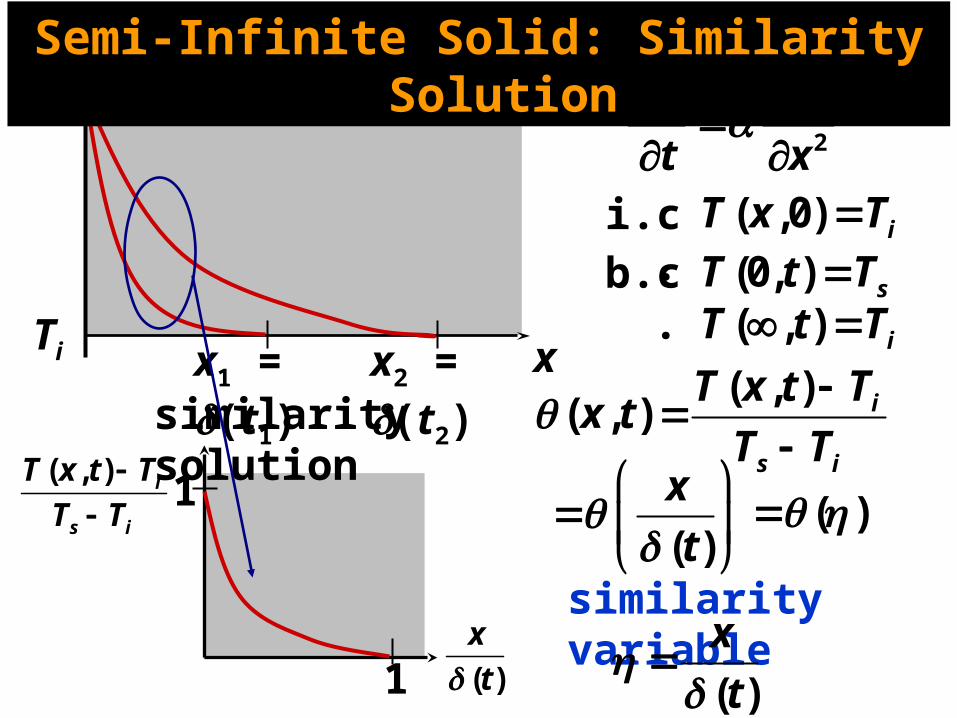
( , ) i
s i
T x t T
T T
( )
x
t
i.c.b.c.
Ti x
Ts
similarity solution
similarity variable
1
1
x1 = (t1) x2 = (t2)
2
2
T T
t x
( ,0) iT x T(0, ) sT t T( , ) iT t T ( , )
( , ) i
s i
T x t Tx t
T T
( )
x
t
( )
( )
x
t
Semi-Infinite Solid: Similarity Solution

Scaling analysisTs
Tix
x = (t)
2
2
T T
t x
~T
t
T
t
2
2
T T
x x x
2~
T
2~
T T
t
2 ~ t ~ t
Let( )
x
t
2
x
t

2
x
t
T
t
s iT Tt
s i
dT T
d t
1
2 2s i
x dT T
dt t
2
s iT T d
t d
T
x
s iT Tx
s i
dT T
d x
1
2s i
dT T
dt
( , )( , ) ( ),i
s i
T x t Tx t
T T

1
2s i
T dT T
x dt
,
2
x
t
2
2
T
x
T
x x
1
2s i
dT T
x dt
1
2s i
d dT T
d d xt
2
2
1
4s i
dT T
t d
2
2
T T
t x
2
s iT T d
t d
2
2
1
4s i
dT T
t d

merge into one
2 0
i.c. ( ,0) :iT x T
b.c. (0, ) sT t T
( , ) iT t T
( , )( , ) i
s i
T x t Tx t
T T
2
x
t
, ( ) 0
0, (0) 1
, ( ) 0
Ts
Tix
x = (t)

Similarity solution
integrating factor
2 0 : (0) 1, ( ) 0 2
e
2
0d
ed
2
1
dC e
d
2
1 d C e d
2
10 0
ud C e du
2
10
( ) (0) uC e du
or
2
10
( ) 1 uC e du
2
10
( ) 0 1 uC e du

erfc: complimentary error function
error function:
2
0
2erf ( ) ,
xux e du
erf ( ) 1
2
10
( ) 0 1 uC e du
2
0 2ue du
1
2C
2
0
2( ) 1 ue du
1 erf ( )
( , )( , ) 1 erf
2i
s i
T x t T xx t
T T t
erfc
2
x
t

Ts
Ti
x1 = (t1) x2 = (t2)x
( , )( , ) i
s i
T x t Tx t
T T
( , ) s s i
s i
T x t T T T
T T
( , )
1 s
i s
T x t T
T T
( , )1 ( , )s
i s
T x t Tx t
T T
1 1 erf ( )
erf2
x
t