transformer design optimization using nested loop
TRANSCRIPT

TRANSFORMER DESIGN OPTIMIZATION
USING NESTED LOOP
MUHAMMAD ZULKIFLI B. ABD HAMID
FACULTY OF ENGINEERING
UNIVERSITY OF MALAYA
KUALA LUMPUR
2018
Univers
ity of
Mala
ya

2
TRANSFORMER DESIGN OPTIMIZATION
USING NESTED LOOP
MUHAMMAD ZULKIFLI B. ABD HAMID
SUBMITTED TO THE
FACULTY OF ENGINEERING
UNIVERSITY OF MALAYA, IN PARTIAL
FULFILMENT OF THE REQUIREMENT FOR
THE DEGREE OF MASTER OF POWER SYSTEM ENGINEERING
2018
Univers
ity of
Malaya

ii
UNIVERSITY OF MALAYA
ORIGINAL LITERARY WORK DECLARATION
Name of Candidate: Muhammad Zulkifli B. Abd Hamid
Matric No: KMA150017
Name of Degree: Master of Power System Engineering
Title of Project Paper: TRANSFORMER DESIGN OPTIMIZATION USING NESTED
LOOP
Field of Study: 132kV Power Transformer
I do solemnly and sincerely declare that:
(1) I am the sole author/writer of this Work;
(2) This Work is original;
(3) Any use of this work in which is copyright exist was done by way of fair dealing and for
permitted purpose and any excerpt or extract form, or to reference to or reproduction of any
copyright work has been disclosed expressly and sufficiently and the title of the Work and its
authorship have been acknowledge in this Work;
(4) I do not have any actual knowledge nor do I ought reasonably to know that the making of
this work constitutes an infringement of any copyright work;
(5) I hereby assign all and every rights in the copyright to this Work to the University of
Malaya (“UM”) and myself who henceforth shall be the owner of this copyright in this Work
and that any reproduction or use in any form or by any means whatsoever is prohibited without
the written consent of University of Malaya and myself having been first had and obtained;
(6) I am fully aware that if in the course of making this Work I have infringed any copyright
whether intentionally or otherwise, I may be subject to legal action or any action as may be
determined by myself and University of Malaya.
Candidate‟s Signature: Date:
Subscribed and solemnly declared before,
Witness Signature: Date:
Name:
Designation:
Univers
ity of
Mala
ya

iii
ABSTRACT
This paper presents Power Transformer design using Nested Loop by optimizing the
important parameters but keeping in sight the guidelines of the International Electro
Technical standards and fundamental Power Transformer specification in general. The
result obtained by using the Nested Loop optimization have been compared with the
result obtained using conventional calculation method (CCM). Using the same sets of
parameters, it is evident that the parameters applying the Nested Loop have been
optimized in comparison to the parameters in CCM. The result of CCM and Nested Loop
have been obtained by coding in MATLAB which is the first effort thus far in the
industries in Malaysia. The presented paper provides convenient, accurate, fast and
reliable solution to overcome any issues related to the optimization of 132kV
Transformer with several listed design options and it fulfills the criteria or compatible
with any kinds of Transformer needs by the global grid power system. Hence, this paper
demonstrates a better and efficient solution for Power Transformer design using the
Nested Loop optimization techniques.
Univers
ity of
Mala
ya

iv
ABSTRAK
Penulisan ini mempersembahkan rekabentuk Alatubah Kuasa yang mengaplikasikan
teknik Nested Loop dengan mengoptimumkan parameter-parameter penting kepada
alatubah disamping mengekalkan keperluan standard IEC (International Electro
Technical) dan spesifikasi asas alatubah kuasa secara umum. Perbandingan keputusan
yang diperolehi menggunakan teknik pengoptimuman Nested Loop telah dibandingkan
dengan kaedah kiraan konvensional (CCM). Menggunakan set parameter yang sama,
ternyata bahawa pengaturcaraan yang mengaplikasikan Nested Loop adalah lebih
optimum berbanding CCM. Perbandingan keputusan ini telah diperolehi dengan
menggunakan kaedah pengaturcaraan didalam perisian MATLAB yang mana pertama
kali diperkenalkan didalam industri Alatubah kuasa di Malaysia ini. Penulisan ini
menawarkan solusi yang mudah, cepat, tepat dan terbukti dalam menyelesaikan isu
pengoptimuman yang berkaitan dengan Alatubah 132kV dengan penyenaraian beberapa
pilihan rekabentuk dan memenuhi kriteria atau sepadan dengan keperluan alatubah ynag
berada di dalam system grid kuasa secara global. Secara keseluruhannya, penulisan ini
mempamerkan solusi yang lebih baik dan effisyen dengan cara pengoptimuman Alatubah
kuasa menggunakan teknik Nested Loop.
Univers
ity of
Mala
ya

v
ACKNOWLEDGEMENT
I would like to express my upmost gratitude to Allah s.w.t for His abundance of givings
and to guides all of us to Jannah, Insya Allah. Firstly, to my supervisor, Associate Prof.
Dr. Jievan A/L Kaneson for his calmness, brilliance and guidance to complete this
dissertation. This work will not stop here and will be the passage through for the next
development phase. To the most important family members especially my mother Datin
Hjh. Jamiah Binti Sanusi who has given me support especially during the hard times
when our father passed away during the 1st
semester of this Master degree. To the mother
of our 3 happy children, my wife, thank you for the support, and sacrifices made in order
to complete this whole journey and to have a better life ahead. To the company I am
working and earning right now Malaysia Transformer Manufacturing Sdn Bhd, thank you
for the knowledge and research platform that constitutes to the important content for this
paper. Finally to the viewers of this paper, please use it with health.
Univers
ity of
Malaya

vi
TABLE OF CONTENT
Page
DECLARATION ii
ABSTRACT iii
ABSTRAK iv
ACNOWLEDGEMENT v
TABLE OF CONTENT vi
LIST OF FIGURES ix
LIST OF TABLES x
LIST OF SYMBOLS xi
ABBREVIATION xiii
CHAPTER 1: INTRODUCTION
1.1 Introduction 1
1.2 Problem Statement 2
1.3 Objectives 2
Univers
ity of
Mala
ya

vii
1.4 Scope of Work 3
CHAPTER 2: POWER TRANSFORMER (132/33kV) DESIGN
2.1 Introduction 4
2.2 Design Parameter and Electrical Performance of Power Transformer 4
2.3 Transformer Design Optimization Procedure 6
2.4 Nested Loop 8
CHAPTER 3: RESEARCH METHODOLOGY
3.1 Introduction 9
3.2 Transformer Design Mathematical Model 10
3.3 Power Transformer Design Process 30
3.4 Optimization Relation for Magnetic Flux Density and Low Voltage Turn 31
3.5 Pseudo Code for the Overall Optimization Algorithm 31
Univers
ityof
Malaya

viii
CHAPTER 4: RESULT OF TRANSFORMER DESIGN OPTIMIZATION
4.1 Introduction 33
4.2 Conventional Calculation Method (CCM) of Power Transformer Design 32
4.3 Nested Loop Optimization of Power Transformer Design 34
4.4 Result Comparison between CCM (Conventional Calculation Method) 38
And Nested Loop Optimization
CHAPTER 5: CONCLUSION AND FUTURE WORK
5.1 Conclusion 42
5.2 Future Work 43
REFERENCE 44
Univers
ity of
Mala
ya
ix
LIST OF FIGURES
Figure No. Page
2.1 Design Flow Chart for Transformer Design Optimization 7
2.2 Automatic Design Optimization 7
2.3 Structure of Nested Loop 8
3.1 Delta Connection 11
3.2 Star Connection 11
3.3 Insulation Distance 16
3.4 CTC Copper Conductor Dimension 18
3.5 Bunch Copper Conductor Dimension 19
3.6 Dimension of the Core and Windings 23
3.7 Power Transformer Design Process 29
3.8 Optimization code for the Magnetic Flux Density and LV Number of Turn 30
3.9 Simplified Pseudo Code for Overall Optimization Algorithm 30
4.1 Prompt Data Pop-Up for Optimization Criterion 35
4.2 Prompt Data Acquisition for Optimization Criterion of Core Diameter 35
4.3 Prompt Data Acquisition for Optimization Criterion of LV Turn 36
4.4 Convergence Characteristic of Nested Loop Optimization 37
Univers
ity of
Mala
ya

x
LIST OF TABLES
Table No. Page
3.1 Insulation Distance 14
3.2 Winding End to Upper Yoke Distance 14
3.3 Winding End to Upper Lower Yoke Distance 15
3.4 Winding Top End Insulation Distance 15
3.5 Winding Bottom End Insulation Distance 15
3.6 Main Duct Insulation Distance 15
3.7 Main Duct Insulation Distance 16
3.8 Core and Windings Total Dimension 20
3.9 Dimension of the Core and Windings 23
4.1 Conventional Calculation Method Design Parameters 33
4.2 Conventional Calculation Method Electrical Performance 33
4.3 Result of Nested Loop Optimization Design Parameters 33
4.4 Convergence Characteristic of Nested Loop Optimization 36
4.5 Result of Comparison between Conventional Calculation Method 37
And Nested Loop Optimization
4.6 Result of Comparison between Conventional Calculation Method 38
And Nested Loop Optimization Electrical Performance
4.7: Result of Comparison between CCM and Nested Loop 39
Optimization Electrical Performance
Univers
ity of
Mala
ya

xi
LIST OF SYMBOLS
𝐸 Voltage applied to the primary
𝑘 Factor (for rectangular waves)
𝐵𝑀 Maximum flux density
𝑁 Number of primary turns
𝐴𝑐 The cross sectional area (cm²)
𝑓 Frequency of operation (Hz)
𝑊𝐴 Core window area (Circular mils)
𝐴𝐶 The effective cross sectional area, in cm²
𝑃0 Output power (W)
∆𝐵 Flux density swings (Tesla)
𝑓𝑆𝑊 The switching frequency (Hz)
𝐾 The winding factor
𝑃𝑤 Total winding losses (W)
𝐼𝑝2𝑅𝑝 The primary and secondary rms current (A)
𝐼𝑠2𝑅𝑠 The primary and secondary dc resistance (Ω)
𝑃𝑤 Copper conductor or winding losses (W)
𝐾𝑟 AC resistance coefficient (Rac/Rdc)
𝜌 The core permeability
𝐴𝐶 The effective cross sectional area, in cm²
𝑉Ø The rated phase voltage, kV
𝑉𝐿𝐿 The rated line to line voltage, kV
Univers
ity of
Mala
ya

xii
𝑆 The rated apparent power, VA
𝐼Ø The rated phase current, A
𝐼𝐿𝐿 The rated line current, A
𝑉∅ The phase voltage of the Low Voltage side.
Univers
ity of
Mala
ya

xiii
LIST OF ABBREVIATIONS
CCM Conventional Calculation Method
C.S.A Core Cross Sectional Area
LV Low Voltage
HV High Voltage
TER Tertiary Voltage
IEC Electro-Technical Committee
BIL Basic Insulation Level
DIL Dielectric Insulation Level
Univers
ity of
Mala
ya

1
CHAPTER 1
INTRODUCTION
1.1 Introduction
An optimum design of Transformer depends on combination of few important factors
namely the minimization of active part cost, minimization of active part mass,
minimization of total owning cost, and minimization of manufacturing cost as well as
maximization of transformer apparent power. One of the challenges of such an objective
function is that the transformer manufacturing cost depends on the cost of the material
(copper, aluminum, steel, etc.) that are stock exchange commodities with fluctuating
prices on the world market [1].
An early attempt was done which described a method for design optimization by
computer. It utilizes a routine called “Monica”, which is use to guide the choice of the
independent variables in such way that the optimum, usually the lowest cost design, is
reached. In essence, this routine does self-optimize its design. The paper shows none of
the design interaction between the designer and the program [2].
The choices of the right core, winding and insulation materials and their subsequent
sizing and geometry play a vital role in the final performance of these transformers. The
objective is to use the best practices obtained from this study in order to help in the
development of the computer aided design tools which in the end objective of the design
process, in order to facilitate the user to try out combinations of the materials and the
design methodology in the medium frequency high power design space and come out
with optimal design [3].
1.2 Proposed Method
Univers
ity of
Mala
ya

2
The nested for loop was developed in 1984 after other earlier programming environment.
It was developed to execute a group of statements in a loop for a specified number of
times. To iterate over the values of a single column vector, first transposed it to create a
row vector.
Univers
ity of
Mala
ya

2
To iterate over the values of a single column vector, first transposed it to create a row
vector. With a high reputation, MATLAB program will be tested to perform engineering
related task in order to test its performance.
1.3 Problem Statement
For Transformer rating up to 132kV voltage levels, it is essential to have a well optimized
design. Many industrial design fatal error in the past were caused by the wrong decision
making during the first design stage. The occurrence of such mistake have emphasized
the importance of design and development process study. The tradition product design
technique involves in trial-and-error design sheets and testing methodology to synthesize
a set of promising Transformer design that attain the targeted results. However, this
technique is time consuming and costly. An alternate way is the top-down reverse
engineering and approach which couples with the proven Nested Loop (MATLAB)
technique to identify the optimal structure of the Transformer design.
1.4 Objectives
The objective of this study are:
1. To design a 132kV Power Transformer
2. To optimize the design by using the Conventional Calculation Method (CCM)
and the Nested Loop Algorithm
3. To compare the result obtained using CCM and Nested Loop
Univers
ity of
Mala
ya

3
1.5 Scope of Works
This study was carried out by designing a 132kV Transformer for a designated TNB
substation. An excel sheet with formulas was developed for the CCM while the
MATLAB software was used for the programming of the transformer design. The initial
transformer design was then optimized by using the Nested Loop to obtain the best Core
parameter, number of Low Voltage turns, Impedance and Reactance value as specified by
the customer. Hence the overall parameter is also computed and compared.
Univers
ity of
Mala
ya

4
CHAPTER 2
POWER TRANSFORMER DESIGN
2.1 Introduction
It has been recorded in history as Power Transformer being the leading and essential to
Power Grid system. With its primary power source conversion from primary to secondary
stage utilizing few important principle of transforming voltage together with isolating
electrical and noise decoupling. The main idea for Transformer to operate is by supplying
energy to the load efficiently. The challenge whereby consistence as supplying bulk
electrical machine with very low frequency can be very high staking risk. The concept of
grasping a reduced size, lesser losses, greater efficiency and lesser volume solid state
Transformer may be achieve in one or a mixture of this three criteria: (1) Modification of
the structural core and winding, (2) Manipulating the flux density of the structural core or
(3) Manipulating the temperature where the winding is operating [4].
2.2 Design Parameters and Electrical Performance of Power Transformer
A Power Transformer design is determined by few terms, which are Core Diameter, Low
Voltage number of Turn (LV Turn), Magnetic Flux density (BFinal), Voltage Per Turn, Core
Weight, No Load Loss, Impedance and Load Losses. The terms are defined as follows:
A. The connection of the term equation comprising voltage (𝐸), Flux Density (𝐵𝑀),
and Frequency (𝑓) is defined by the experiments of the Faraday‟s Law [4]:
𝐸 = 𝑘𝐵𝑀𝑁𝐴𝑐 𝑓 𝑥 10−8
(1) Univ
ersity
of M
alaya

5
Where
𝐸 is primary voltage
𝑘 is 4.0 (for rectangular waves)
𝐵𝑀 is maximum flux density
𝑁 is number of primary turns
𝐴𝑐 is the cross sectional area (cm²)
𝑓 is the Frequency of operation (Hz)
B. Core Size Selection
Transformer Core solid and the thickness were determined. In Power Transformers, tally
these losses to no-load losses, which occur when the Transformer is linked to a voltage
source and give back substantially to growth cost of the Transformer [5]. Next, designers
will look into the supplying output power and also the generated frequency in the system.
The structure of the core considering the winding for it to be filled must be optimized in
order to reduce leakage of flux. The selection of core and winding need to be balanced as
core sectional area and winding diameter has to be suitable to avoid further difficulties
during manufacturing. The power handling capability of a core can easily verify by this
core area product (WA x AC). A rough indication of the required area product is given by
[4]:
𝑊𝐴 𝐴𝐶 = 𝑃0
𝐾∆𝐵𝑓𝑆𝑊
4
3
Where
𝑊𝐴 is core window area (Circular mils)
𝐴𝐶 is the effective cross sectional area, in cm²
𝑃0 is output power (W)
∆𝐵 is flux density swings (Tesla)
𝑓𝑆𝑊 is the switching frequency (Hz)
𝐾 is the winding factor
(2)
Univers
ity of
Mala
ya

6
C. Winding Losses
Winding losses of two Transformer carrying an AC current can be considered as
𝑃𝑤 = 𝐼𝑝2𝑅𝑝 𝑥 𝐼𝑠
2𝑅𝑠
Where
𝑃𝑤 is total winding losses (W)
𝐼𝑝2𝑅𝑝 is the primary and secondary rms current (A)
𝐼𝑠2𝑅𝑠 is the primary and secondary dc resistance (Ω)
However, for a streamlined argument or study, designer can consider the succeeding
calculation, which has been shown by Petkov [4]:
𝑃𝑤 = 𝐾𝑟 𝑥 𝜌 𝑥𝐼2
𝑟𝑚𝑠
𝐴𝑐
Where
𝑃𝑤 is copper conductor or winding losses (W)
𝐾𝑟 is an AC resistance coefficient (Rac/Rdc)
𝜌 is the core permeability
𝐴𝐶 is the effective cross sectional area, in cm²
2.3 Transformer Design Optimization Procedure
There has been a proposal to design Transformer applying the automatic optimization
using shell Transformer. The design constraint is focused on the core lamination. When
the area is decreasing, its dimension in lamination can be increased. The volume increase
gradually until the set value of temperature is obtained. The Figure 2.1 shows the
flowchart of designing the Transformer. Zooming in the design flowchart, another
optimization criterion which chosen as subject for detailed were presented by another
research. Focusing on the core type medium frequency and proposed an optimization
flowchart which is indicated in Figure 2.2. In this automatic design optimization, the one
turn voltage of primary winding is used as the key parameter to change the core and the
winding design till the optimized result are obtained [3].
(3)
(4)
Univers
ity of
Mala
ya

7
Figure 2.1: Design Flow Chart for Transformer Design Optimization
Figure 2.2: Automatic Design Optimization
Univers
ity of
Mala
ya

8
2.4 Nested Loop (MATLAB)
Cleve Moler invented the program in the year of 1970. The program invented were
rendered from the FOTRAN with it sub program identified as LINPAK and EISPACK
utilizing linear and eigenvalue method. It was re-written in C in the 1980‟s with more
functionality, which includes plotting routines [6].
The statement inside of a nested loop can be any valid statement, including any selection
statement. For example, there could be an „if‟ or „if-else‟ statement as the action, or part
of the action in a loop. For example if the data for any type of analysis loaded into a
matrix variable. The script will find the size of the matrix and then loops through all the
elements in the matrix using by using the nested loop. The outer loop iterates through the
rows and the inner loop iterates through the columns [7].
Loops and conditional statement can be nested within other loops or conditional
statements. This means that loops and/or conditional statement can start (and end) within
another loop or conditional statement. There is no limit to the number of loops and
conditional statement that can be nested. Figure 2.3 show the structure of a nested for-end
loop within another for-end loop. In the loops shown in this figure, if for example n=3
and k=4, then first k=1.Next, k =2, and the nested loop executes 4 times with h =1, 2, 3,
4. Finally k=3, and the nested loop executes 4 times again. Every time a nested loop is
typed, MATLAB automatically indents the new loop relative to the outside loop. Nested
loop and conditional statement are demonstrated in the following chapter [8].
Figure 2.3: Structure of Nested Loop
Univers
ity of
Mala
ya

9
CHAPTER 3
RESEACRH METHODOLOGY
3.1 Introduction
The transformer is an electromagnetic conversion device in which electrical energy
received by the primary winding is first converted into magnetic energy which is
reconverted back into a useful electrical energy in other circuit (secondary winding,
tertiary winding, etc.) Thus, the primary and secondary winding are not connected
electrically, but coupled magnetically. A Transformer is termed as either a step down or a
step up transformer depending on whether the secondary voltage is higher or lower than
the primary voltage, respectively. Transformer can be used as either step-up or step-down
voltage depending upon the need and application. Hence, their windings are referred as
high-voltage/low-voltage or high tension/low tension winding in place of primary or
secondary windings [9].
From a maker‟s perspective, it is useful to design and produce a set range of Transformer
sizes. Usually, the terminal voltages, VA rating and frequency are specified. In the
conventional method of Transformer design, these specification decide the materials to be
used and their dimension. The methodology has been used as a strategy tools for teaching
in engineering school. However, by designing to rated specification, consideration is not
openly given to what materials and sizes what are actually available. It is possible that an
engineer having designed a Transformer, maybe then find the material sizes not exist.
The engineer may then be forced to use available materials. Therefore, the performance
of the actual Transformer built is likely to be different from that of the design
calculations. Thus, the optimized design of the magnetic component is not based on
selection of the right magnetic core but on the definition of its best dimensions [10].
Univers
ity of
Mala
ya

10
In the reverse design approach, the physical characteristics and the specification are
determined by evaluating the dimensions of the windings and core. By manipulating the
amount and type of material actually to be used in the transformer construction, its
performance can be determined. This is essentially the opposite of the conventional
Transformer design method. It allows for the customized design, as there is considerable
flexibility in meeting the performance required for a particular application. [11].
In this chapter, Transformer design terminology, Transformer design steps and review of
the optimization technique are explained.
3.2 Transformer Design Mathematical Model
The Transformer performance is determined by few terminologies, which are Voltage
requirement and calculation, etc. The terminologies are defined as follows:-
1. Voltage Requirement and Calculation
Determine the HV and LV Winding, Line Voltage and Phase Voltage. Phase Voltage is
required for winding turn calculation. For Star connection of three phase Transformer,
phase voltage is equal to 1
3 line voltage. For delta connection, phase voltage is equal to
line voltage. The formula is as follow:
( Y- Vector Group)
𝑉Ø =1
3 𝑉𝐿𝐿
( ∆- Vector Group)
𝑉Ø = 𝑉𝐿𝐿
where 𝑉Ø is the rated phase voltage, kV and 𝑉𝐿𝐿 is the rated line to line voltage.
(1)
(2)
Univers
ity of
Mala
ya

11
2. Current Calculation
Determine the HV and LV Winding, Line Current and Phase Current. Phase Voltage is
required for winding type and its carrying capacity. For Star connection of three phase
Transformer, phase current is equal to line current. For delta connection, phase current is
equal to 1
3 line current. The formula is as follow:
( Y- Vector Group)
𝐼Ø = 𝐼𝐿𝐿 = 𝑆
3𝑉𝐿𝐿
( ∆- Vector Group)
𝐼Ø =𝐼𝐿𝐿
3
= 𝑆
3𝑉Ø
where 𝑆 is the rated apparent power , VA and 𝐼Ø is the rated phase current and 𝐼𝐿𝐿 is the
rated line current.
Figure 3.1: Delta Connection Figure 3.2: Star Connection
(3)
(4)
Univers
ity of
Mala
ya

12
3. Core Diameter Estimation and Induced Voltage Constraint
3.1 Core Diameter Estimation
Usually core are made of silicon steel or CRGO (Cold Rolled Grain Oriented) steel that is
used to create alternating magnetic circuit for Transformer. The calculation is as follow:-
Diameter of the Transformer Core, D
= 𝑇𝑖𝑐𝑘𝑛𝑒𝑠𝑠 𝑜𝑓 𝐶𝑅𝐺𝑂 𝑃𝑙𝑎𝑡𝑒𝑠 𝑊𝑖𝑑𝑡1𝑥 𝑁𝑢𝑚𝑏𝑒𝑟 𝑜𝑓 𝐵𝑙𝑎𝑑𝑒𝑠 𝑊𝑖𝑑𝑡1
+ 𝑇𝑖𝑐𝑘𝑛𝑒𝑠𝑠 𝑜𝑓 𝐶𝑅𝐺𝑂 𝑃𝑙𝑎𝑡𝑒𝑠 𝑊𝑖𝑑𝑡2𝑥 𝑁𝑢𝑚𝑏𝑒𝑟 𝑜𝑓 𝐵𝑙𝑎𝑑𝑒𝑠 𝑊𝑖𝑑𝑡2
+ 𝑇𝑖𝑐𝑘𝑛𝑒𝑠𝑠 𝑜𝑓 𝐶𝑅𝐺𝑂 𝑃𝑙𝑎𝑡𝑒𝑠 𝑊𝑖𝑑𝑡3𝑥 𝑁𝑢𝑚𝑏𝑒𝑟 𝑜𝑓 𝐵𝑙𝑎𝑑𝑒𝑠 𝑊𝑖𝑑𝑡3
+ 𝑇𝑖𝑐𝑘𝑛𝑒𝑠𝑠 𝑜𝑓 𝐶𝑅𝐺𝑂 𝑃𝑙𝑎𝑡𝑒𝑠 𝑊𝑖𝑑𝑡(𝑛) 𝑥 𝑁𝑢𝑚𝑏𝑒𝑟 𝑜𝑓 𝐵𝑙𝑎𝑑𝑒𝑠 𝑊𝑖𝑑𝑡(𝑛)
OR to select the Core Diameter value based on experience or some empirical formula [9].
3.2 Core Cross Sectional Area (Core C.S.A)
In design, effective section is determined by the Core Cross Sectional area. At certain
condition of the core diameter, the more stacks the bigger the effective section area is.
Stacked factor selection related to the thickness, flatness of silicon steel and varnish film
thickness. Space actual factor reduces as coating of the non-magnetic insulation were
measured together as thickness. Usually with the value of 0.97.
𝐶𝑜𝑟𝑒 𝐶. 𝑆. 𝐴 =𝜋(𝐷2)
4𝑥 𝑆𝑡𝑎𝑐𝑘𝑒𝑑 𝐹𝑎𝑐𝑡𝑜𝑟 𝑥 𝑈𝑡𝑖𝑙𝑖𝑧𝑎𝑡𝑖𝑜𝑛 𝐹𝑎𝑐𝑡𝑜𝑟
where 𝐷 is the diameter of the Transformer core.
3.3 Induced Voltage Constraint
For a sinusoidal waveform, the rms value of the induced voltage in the primary winding
is given by
𝐸𝑝 = 2𝜋 𝑥 𝐹𝑟𝑒𝑞 𝐻𝑧 𝑥 𝑁𝐿𝑉 𝑥 𝐵 𝑥 𝐶𝑜𝑟𝑒 𝐶. 𝑆. 𝐴
(5)
(6)
(7)
Univers
ity of
Mala
ya

13
where 𝐹𝑟𝑒𝑞 𝐻𝑧 is the operating frequency , 𝑁𝐿𝑉 is the number of Turn in the LV
Winding, and 𝐵 is the maximum value of flux density. Rated frequency for Malaysia is
50 Hz whereas for the Maximum Flux Density is around 1.7 Tesla. For developing large
Transformer and Reactors, it is necessary to know the distribution of the magnetic
leakage field to calculate the electro-dynamic forces and the stray losses due to eddy
currents in the winding conductors and in steel part such as core, tanks, pressing beams
and others [12].
Cold Rolled Grain Oriented (CRGO) has a unique saturation flux density value up to a
value of 2.0T whereas 1.9T are the value of saturation of the knee point to begin
appearing. The severity of the over-excitation conditions as stated by the user will
determine the operating points (the mutual flux density, B indicated by the peak value).
3.4 Preliminary Calculation of the Low Voltage Winding Turn (𝑁𝐿𝑉)
𝑁𝐿𝑉 =𝑉∅
𝐸𝑝
where 𝑉∅ is the phase voltage of the Low Voltage side.
According to the formula of the Low Voltage Winding Turn 𝑁𝐿𝑉 , it is not necessarily an
integer. If rounding down to an integer, magnetic flux density, B will be bigger than
preliminary calculation. If rounding up to an integer, magnetic flux B, will be smaller
than the preliminary calculation.
3.4 Calculation of the High Voltage Winding Turn (𝑁𝐻𝑉)
Usually HV winding has tap. Calculate the number of Turn according to the tapping
phase voltage. Calculate the biggest number of tapping turn at first:-
𝑁𝐻𝑉 𝑀𝐴𝑋 =𝑉∅ 𝑀𝐴𝑋
𝐸𝑝
(8)
(9)
Univers
ity of
Mala
ya

14
Consequently for the Nominal Tap Voltage and Minimum Tap Voltage
𝑁𝐻𝑉 𝑁𝑂𝑅𝑀 =𝑉∅ 𝑁𝑂𝑅𝑀
𝐸𝑝
𝑁𝐻𝑉 𝑀𝐼𝑁 =𝑉∅ 𝑀𝐼𝑁
𝐸𝑝
where, 𝑁𝐻𝑉 𝑁𝑂𝑅𝑀 is the number of Turn in the HV for Nominal Voltage and 𝑁𝐻𝑉 𝑀𝐼𝑁 is
the number of Turn in the HV for Minimum Voltage.
4. Main Insulation Distance
4.1 Clearance of Inner Winding to the Core Distance, A1
Voltage Class, (kV) 11
Dielectric Level (AC/LI,(kV)) 95/28
Insulation Distance (mm) 17
Thickness of Cylinder (mm) 3 and 5
Quantity of Cylinder 3
Table 3.1: Insulation Distance
4.2 Winding End to Upper Yoke Distance, A2
Voltage Class, (kV) 132 33 11
Dielectric Level (AC/LI,(kV)) 650/275 200/72 95/28
Insulation Distance (mm) 100 100 100
(10)
(11)
Univers
ity of
Mala
ya

15
Table 3.2: Winding End to Upper and Lower Yoke Distance
4.3 Winding End to BottomYoke Distance, A3
Voltage Class, (kV) 132 33 11
Dielectric Level (AC/LI,(kV)) 650/275 200/72 95/28
Insulation Distance (mm) 100 100 100
Table 3.3: Winding End to Upper and Lower Yoke Distance
4.4 Winding Top End Insulation Distance, A4
Voltage Class, (kV) 132 33 11
Dielectric Level (AC/LI,(kV)) 650/275 200/72 95/28
Insulation Distance (mm) 220 220 220
Table 3.4: Winding Top End Insulation Distance
4.5 Winding Bottom End Insulation Distance, A5
Voltage Class, (kV) 132 33 11
Dielectric Level (AC/LI,(kV)) 650/275 200/72 95/28
Insulation Distance (mm) 150 150 150
Table 3.5: Winding Bottom End Insulation Distance
4.6 Main Duct Insulation Distance, A6
Voltage Class, (kV) 132 33
Dielectric Level (AC/LI,(kV)) 650/275 200/72
Univers
ity of
Mala
ya

16
Insulation Distance (mm) 50 16
Thickness of Cylinder (mm) 2 and 3 3
Quantity of Cylinder 4 1
Table 3.6: Main Duct Insulation Distance
Figure 3.3: Insulation Distance
4.7 Phase to Phase Distance
Voltage Class, (kV) 33
Dielectric Level (AC/LI,(kV)) 200/72
Insulation Distance (mm) 36
Table 3.7: Main Duct Insulation Distance
TRANSFORMER_CORE
TR
AN
SF
OR
ME
R_
CO
RE
A1
TER LV1 LV2 HV REG
A2 A4
A5
A6
A3
Univers
ity of
Mala
ya

17
5. Winding Calculation
5.1 Low Voltage Winding Design
Usually, when copper type conductor section area is smaller than 2mm², use round
enameled wire. However if the conductor width is up to and including 15mm and the
thickness is up to and including 4.3mm, use either paper wrapped flat wire or glass fiber
wrapped flat wire. The same case for Aluminum type, when it is smaller than the 8mm²,
use enameled round wire. Nevertheless, if the conductor width is up to and including
17mm and the thickness is up to and including 5.3mm, use either paper wrapped flat wire
or glass fiber wrapped flat wire. The complicated shape of the insulation system is such
that it has to relieve the electric stress at the end of the winding and it does this by
distributing the potential and hence stress around a labyrinth of duct and barriers [13].
5.1.1 Current Density Selection
Current density of the conductor is determined by the load loss, winding temperature rise
and dynamic stability and thermal stability when short circuited the second winding.
Usually the current density of the copper conductor is up to and including 3.5A/mm²
without exceeding the temperature rise limits, while current density of copper conductor
is up to and including 2.0mm². One consequential problem is that short-circuit forces and
stresses in the windings have increased also [14].
5.1.2 Current Density Calculation
𝐼(𝐿𝑉 𝐶𝑈𝑅𝑅𝐸𝑁𝑇 𝐷𝐸𝑁𝑆𝐼𝑇𝑌) =𝐼Ø𝐿𝑉
𝐴(𝐿𝑉 𝐶𝑂𝑁𝐷𝑈𝐶𝑇𝑂𝑅 )
The edges of the conductor appears due to manufacturing casting copper curvy radius of
0.6 – 1.2mm which in turn elude high-pitched corners possibly damaged the insulation
(12)
Univers
ity of
Mala
ya

18
layer and to lessen the high electric stress levels, and as calculated above eventually
requires a smaller area of the conductor.
5.1.3 Paper Cover Insulation on the Conductor
An upper dimension of the insulation wrapping tend to upgrade the withstand pressure
but deteriorates heating values compared to the copper and the nearby liquid insulated
area. A firm layer of wrapping are necessary from existing structure strength point of
views. Convection process is one of the way of natural heat transfer through the oil
channel provided the gap in between is properly prepared. Mid-depth area of the
windings should have a bigger gap in between the conductor called the ducts for effective
cooling. Axial ducts reacts as the cooling agent from internal side of the winding as well
as the outer of the windings.
Important factor of thermal and dielectric rules in Transformer manufacturing will decide
for the insulation in between the winding disc. Thermal condition normally are the
deciding factor for the Low Voltage winding side. Convection process is one of the way
of natural heat transfer through the oil channel provided the gap in between is properly
prepared. Mid-depth area of the windings should have a bigger gap in between the
conductor called the ducts for effective cooling. Axial ducts reacts as the cooling agent
from internal side of the winding as well as the outer of the windings.
Axial Dimension
Radial
Dimension
Axial
Dimension
Bare
Radial
Dimension
Bare
Univers
ity of
Mala
ya

19
Figure 3.4: CTC Copper Conductor Dimension
5.2 High Voltage Winding Design
The section number and layer field strength of High Voltage winding is determined by
voltage level. The Basic Insulation Level (BIL) of 230kVrms/550kVp normally the value
required for 132kV Transformers. The designer will optimize the value to somewhere
around 20% based on details scheming or analysis involving the impact on the inter-turn
disc. Rated voltage and impulse stresses as one of the indication. The selection of the
discs size need to be selected in order for a proper copper width is determined as
designing stage of the Low Voltage Winding. Under few circumstances, if the dimension
chosen is optimum, the winding height need to be indirectly proportional to the number
of turns.
The primary side voltage winding has been proposed to perform as a disc winding with
continuous arrangement. Disc winding with shielding arrangements and interleaved disc
are selected normally for 132kV class transformers. For 220kV voltage level, this
arrangements has been proven to stabilize the stresses appearing along the winding.
5.2.1 Paper Cover Insulation on the Conductor
As stated earlier, the insulation required for any copper conductor on the winding will be
based on the impulse test voltage and the strain in between the conductor turn. Next the
cooling part need to be considered as the ducts will be placed along the disc. Designers
have the flexibility in modifying the gaps in between the two direct continuous disc. Line
end and neutral end tends to have difference in the dimension of the space as it will
undergo testing with overvoltage conditions and will witness a sharp ramp in the
waveform.
Univers
ity of
Mala
ya

20
Figure 3.5: Bunch Copper Conductor Dimension
5.3 Height of the Low Voltage and High Voltage Winding
The rule of thumb in order to maintain the dimension are to make sure that the height of
LV and HV are the same. However, there are sample cases which the LV windings are
resize in order to reduce the strain of over-voltages and voltage impulse. In some design,
the same identical dimension of windings are located in middle level line to reduce axial
pressure. The electric field leakage is less at the dominant dimension area with less
number of pressure acting on it. Such short circuit pressure acting on typical secondary
level winding or Low Voltage in a helical and layer shape.
5.4 Core and Windings Total Dimension
As designer establish the core dimension as well as the winding size which is derived
from the conductor size and copper area, now is where the core winding combination
Axial
Dimension
Bare
Axial
Dimension
Radial
Dimension
Radial
Dimension Bare
Univers
ity of
Mala
ya

21
begin. The important mean diameter and whole radius of windings layer are given
below:-
ITEMS
CLEARANCE (mm)
GAP (mm)
DIAMETER
(mm)
1 684
2 21 Tertiary Winding 705
3 726
4 16 Tertiary to Low Voltage Winding 742
5 758
6 38 Low Voltage 1 796
7 834
8 16 Low Voltage 1 to Low Voltage 2 850
9 866
10 38 Low Voltage 2 Winding 904
11 942
12 50 Low Voltage to High Voltage 992
13 1042
14 110 High Voltage Main Winding 1152
15 1262
16 40 HV to Regulating Winding 1302
17 1342
18 11 Regulating Winding 1353
19 1364
20 Phase to Phase Distance 36
Table 3.8: Core and Windings Total Dimension
The examples shown in the calculation consider the gap dimension of both HV and LV
based on their respective radial dimension. It should be noted that the distance required in
Univers
ity of
Mala
ya
22
between core to tertiary winding for 33kV class is specified as 21mm with 70kV
rms/10kVp insulation level. It is different cases for a less voltage level since the value of
gap and mechanical consideration will be observed to decide the distance in between
winding and core. It should be noted that the Basic Insulation Level can be slightly higher
than the specified level due to consideration of surge voltage in between windings thus
deciding the gap of inner core towards innermost winding. For example, looking on the
distance between phases in HV winding as static and the other distance from the HV
static in comparison to other winding should be made larger in any adjacent direction.
Lightning impulse of the HV winding is important and as deciding factor to determine the
dimension of the HV to LV gaps. Based on the testing procedure, when lightning impulse
is conducted on HV side, other terminal will be grounded. To be on the save side, the
dimension gap in between phases are kept larger compared to the LV gap. In some
design, Basic Insulation Level are specified as one way for the maker to tell the phase to
phase distance. As the existing electric field calculation software could only take
maximum electric field strength as the insulation criterion, which is redundant and with
low economic feasibility [15].
The insulation height in between winding and core is a strict requirements adhering to the
dielectric insulation level, winding compact clamping as well as thermal consideration.
This will in turn decide the highest or maximum dimension of the end insulation that can
be made through early designing process. The specified Basic Insulation Level of the
132kV side are 550kVp and 230kV rms. From this value, the insulation from the upper
top yoke up to the distance between phases can be computed. Another important criteria
in deciding the specification of the insulation are the 3 phase top leads of HV winding.
Winding support will be put to ensure all the winding is clamped all together to avoid any
movements to the winding. Winding support which is made out of insulation pressboard
is suit for the design since it has a good mechanical structure strength. However, due to
the dimension or size, it may cause a problem during design stage because it will affect
the height and affecting clearances. The whole transformer body also was design in a way
Univers
ity of
Mala
ya

23
that the oil will flow through in between the windings and directed in a direction of top to
the bottom for efficient cooling.
Upper and lower lead voltages are of 33kV voltage of 70 kVrms/170 kVp Basic
Insulation Level should sides of delta connection is linked. 70 kV rms/170 kVp Basic
Insulation Level is intended for Neutral connection. Any increase during any over current
or fault condition will be covered under the gap or clearance requirement of
38kVrms/95kVp Basic Insulation Level. The assembled winding need to be strong at the
bottom part. Some area are required for the winding to place perfectly. There are very
little option on selection of space in the bottom. The Neutral terminal will be on the
higher side in order to maintain a line voltage at the winding. There will be specific test
to be performed to test such condition. Designer will have to think with end in mind
when dealing with this condition during designing stage.
Figure 3.6: Dimension of the Core and Windings
5.4.1 Dimension of the Core and Windings
No Location Distance (mm)
TER
LV1
LV2
HV
REG TER
LV1
LV2
HV
REG TER
LV1
LV2
HV
REG TER
LV1
LV2
HV
REG TER
LV1
LV2
HV
REG TER
LV1
LV2
HV
REG
A7 A7
R Y B A8
D Univers
ity of
Mala
ya

24
1 Centre to Centre Distance of the Core
Structure , A7
1400
2 Core Leg Length, A8 1530
3 Core Diameter, D 650
Table 3.9: Dimension of the Core and Windings
6.0 Core Weight and Loss Calculation
𝐶𝑜𝑟𝑒 𝐿𝑒𝑛𝑔𝑡
= 4 𝑥 1
2 𝑥 𝐶𝑜𝑟𝑒 𝐷𝑖𝑎𝑚𝑒𝑡𝑒𝑟 + 3 𝑥 𝐶𝑜𝑟𝑒 𝐿𝑒𝑔 𝐿𝑒𝑛𝑔𝑡
+ (4 𝑥 𝐶𝑒𝑛𝑡𝑟𝑒 𝑡𝑜 𝐶𝑒𝑛𝑡𝑟𝑒 𝐷𝑖𝑠𝑡𝑎𝑛𝑐𝑒 𝑜𝑓 𝑡𝑒 𝐶𝑜𝑟𝑒 𝑆𝑡𝑟𝑢𝑐𝑡𝑢𝑟𝑒)
This calculation demonstrates the equation in order to determine the Core Volume
utilizing the given values at initial stage.
𝐶𝑜𝑟𝑒 𝑉𝑜𝑙𝑢𝑚𝑒 = 𝐶𝑜𝑟𝑒 𝐿𝑒𝑛𝑔𝑡 𝑥 𝐶𝑜𝑟𝑒 𝐶𝑟𝑜𝑠𝑠 𝑆𝑒𝑐𝑡𝑖𝑜𝑛𝑎𝑙 𝐴𝑟𝑒𝑎
𝐶𝑜𝑟𝑒 𝑊𝑒𝑖𝑔𝑡 = 𝐶𝑜𝑟𝑒 𝑉𝑜𝑙𝑢𝑚𝑒 𝑥 𝐶𝑜𝑟𝑒 𝐷𝑒𝑛𝑠𝑖𝑡𝑦
Where the density of the Core Lamination = 7.65 x 10ˉ⁶ kg/mm³
In obtaining the No Load Losses, two modules will be considered, the eddy loss and
hysteresis loss. The losses are calculated using the curves as manufacturer provides it
which take into account few modules. For example, Watt/kg (losses of core lamination)
from the contractor curvature at peak effective flux densities of 1.7 Tesla = 1.2.
(13)
(14)
(15)
Univers
ity of
Mala
ya

25
Limb and yokes are identified to be the greater contributor of the flux loss densities
considering area of flux cross, saturation and others. Hence, a penalty has to be executed
for these area while computing the losses. As a simpler measure, the known factor are
marked as 2.0. Based on the drawing weight of parts can be computed. From an
assumption, the joints add 30% from all the calculation. The core loss be able to be
determined.
𝑊𝑒𝑖𝑔𝑡 𝑜𝑓 𝑡𝑒 𝐽𝑜𝑖𝑛𝑡𝑠 = 0.3 𝑥 𝐶𝑜𝑟𝑒 𝑊𝑒𝑖𝑔𝑡
𝑇𝑜𝑡𝑎𝑙 𝐶𝑜𝑟𝑒 𝐿𝑜𝑠𝑠 = 𝐶𝑜𝑟𝑒 𝑊𝑒𝑖𝑔𝑡 − 𝑊𝑒𝑖𝑔𝑡 𝑜𝑓 𝑡𝑒 𝐽𝑜𝑖𝑛𝑡𝑠
The value that is known to most of the manufacturer are in the area of 1.7 Tesla flux
density that can be define based on constructing factor. The measurement on the
Epstein‟s Test will indicate the flux density when it is built at manufacturer premise.
Here all identified factor during the building of the core will be examined and tested with
the outcome of the values. The building factor need to be considered as 1.3. Therefore
the calculated core loss can be identified.
𝐶𝑎𝑙𝑐𝑢𝑙𝑎𝑡𝑒𝑑 𝐶𝑜𝑟𝑒 𝐿𝑜𝑠𝑠 = 𝑇𝑜𝑡𝑎𝑙 𝐶𝑜𝑟𝑒 𝐿𝑜𝑠𝑠 𝑥 1.2 𝑥 1.3
7.0 Equivalent Circuit: Shunt Branch
The corresponding circuit has per-phase amounts. The shunt branch has few components
in parallel: Rc symbolizes the total core loss and Xm denotes the magnetizing reactance.
𝑅𝑐 =(𝑅𝑎𝑡𝑒𝑑 𝑉𝑜𝑙𝑡𝑎𝑔𝑒)2
𝐶𝑎𝑙𝑐𝑢𝑙𝑎𝑡𝑒𝑑 𝐶𝑜𝑟𝑒 𝐿𝑜𝑠𝑠
𝐼𝑐 =(𝑅𝑎𝑡𝑒𝑑 𝑉𝑜𝑙𝑡𝑎𝑔𝑒)2
𝑅𝑐
The amounts are being designed as stated to the HV side. A higher value of Rc shows
increased steel characteristic degradation of the reluctance linkages from example over
(16)
(17)
(18)
(19)
(20)
Univers
ity of
Mala
ya

26
current withstand pressure between the core building will further overcome the resistance
and increased loss. For a simpler measure, designers refer to a schedule data on the losses
information to establish core losses. There are tendency of higher losses from the single
plate due to jointing. The example of the built core at 1.7 with given flux density as
below
𝑁𝑜 𝐿𝑜𝑎𝑑 𝐶𝑢𝑟𝑟𝑒𝑛𝑡 = 𝐼𝑜 =
𝑉𝐴
𝑘𝑔 𝑥 𝐶𝑜𝑟𝑒 𝑊𝑒𝑖𝑔𝑡
3 𝑥 𝑅𝑎𝑡𝑒𝑑 𝑉𝑜𝑙𝑡𝑎𝑔𝑒
𝑀𝑎𝑔𝑛𝑒𝑡𝑖𝑧𝑖𝑛𝑔 𝐶𝑢𝑟𝑟𝑒𝑛𝑡𝑠 = 𝐼𝑚 = 𝐼𝑜2 − 𝐼𝑐
2
The no-load power factor is as follow
𝐶𝑜𝑠 𝜃0 =𝐼𝑐𝐼𝑜
When material grades are optimized, the lowering in Im can be still be bigger than the
decrease in Ic. It will be computed as the given equation
𝑋𝑚 =𝑅𝑎𝑡𝑒𝑑 𝑉𝑜𝑙𝑡𝑎𝑔𝑒
𝐼𝑚
The single plate has higher effective permeability than the core being built due to jointing
effect from one another. Magnetizing reactance provides for higher effective permeability
based on the equivalent circuit. Both characteristic of magnetic reactance and reluctance
of magnetic circuit are in inversely proportional with regards of the winding.
(22)
(23)
(24)
Univers
ity of
Mala
ya

27
8.0 Leakage Reactance Scheming
A procedure for the determining the reactance is explained here. The inductance in the
design winding taking N turns which flux linkages Ø can be designed based from this
expression.
𝐿 =𝑁∅
𝑖
𝐿 =𝑁𝐵𝐴
𝑖=
𝑁𝜇𝐻𝐴
𝑖=
𝑁𝜇 𝑁𝑖/𝑙 𝐴
𝑖=
𝜇𝑁2𝐴
𝑙
𝐿 =𝜇𝑁2𝐴
𝑙=
𝑁2
𝑙/(𝜇𝐴)=
𝑁2
ℜ
The relationship ∅ = 𝐵𝐴 and 𝐻 = 𝑁𝑖/𝑙 will be utilized, ℜ is the reluctance of the
directive direction of flux and the other marking in the equation. It is a recognized effects
that in the formula, the magnetic densities Ø is connected through whatever number of
𝑁 turns, and 𝑙 turning into overall winding axial dimension. Form the given
formula, 𝑙 comprising flux ∅ through the flux circular shape which connected
throughout the turns. LV and HV windings will be the center point of the field presence
of flux. The relation between LV and HV turns are that half of LV field will be residual
to the HV winding turn. From the observation, this phenomenon can be assume to be
calculated from axial height. Hence the flux lines in the clearance area depending to the
amperes turn will be same. For instance, the magnetizing amperes-turns are neglected if
the LV and the HV ampere-turns which are of same values. In this case the calculation of
the leakage reactance will be solely based on the axial length (heights) which are equal in
terms of flux.
Using the Maxwell‟s ampere-circuital law, are whole sets of connotation assumed to be
equal in the flux lines towards the gap area. It is the same for any direction in the
windings of HV and LV flux lines. As the ampere turn lowered, and the distance is far
away from winding, lower 𝐻 and 𝐵will be recorded. Therefore, having the Current and
Number of turn (Ampere-Turn) and the vector shaping in a trapezoidal form. To establish
a calculation of leakage inductor value, magnetic flux value has to be seen as variable due
to winding dimension across the line. Accordingly, when inductor value is measured as
(25)
(26)
(27)
Univers
ity of
Mala
ya

28
𝜇𝑁2𝐴
𝑙 , the cross sectional area of the flux circular shape area, consisting the secondary
side winding, the clearance and the primary side winding have 1/3 as the calculation
factor.
Also, the formula 𝑙 value in the equation considered to be efficient dimension of the
circular, to be designed by height known as Rogowski factor. Height of the winding will
relate to the factor calculated and the circular flux shape. This also will consider the
linkages between nearby windings and the total manufacturing length.
To compute the effective area as per below formula
𝐴 = 𝜋 𝑥 𝑚𝑒𝑎𝑛 𝑑𝑖𝑎𝑚𝑒𝑡𝑒𝑟 𝑥 𝑟𝑎𝑑𝑖𝑎𝑙 𝑑𝑒𝑝𝑡
The terms conforming to the secondary and primary windings are grew by 𝐴 equal 𝜋
times ΣEATD by equation below
𝐾𝑅 = 1 − 𝑒−𝐻𝑤 /(𝑇1+𝑇𝑔+𝑇2 )
𝜋𝐻𝑤/(𝑇1 + 𝑇𝑔+𝑇2)
And the equivalent axial dimension of the magnetic circular is 𝑙 . The leakage inductor
on going to the primary side will be established (on the primary side).
𝐿 =𝜇𝑁2𝐴
𝑙
The intended circuitry will be seen to the secondary side, the value needs to be multiplied
by
𝑅𝑎𝑡𝑒𝑑 𝑘𝑉𝐿−𝐿 𝐿𝑉 2
𝑅𝑎𝑡𝑒𝑑 𝑘𝑉𝐿−𝐿 𝐻𝑉 2
For example the ration of squares of the line-line voltage of the HV and LV Windings.
The leakage reactance is (referred to the HV side).
(28)
(29)
(30)
(31)
(32)
Univers
ity of
Mala
ya
29
𝑋 = 2𝜋𝑓𝐿
The per-unit overall impedance and reactance value is depended to the true value seen on
the primary side as
𝑅𝑎𝑡𝑒𝑑 𝑘𝑉𝐿−𝐿 𝐿𝑉 2
𝑀𝑉𝐴 3∅
9.0 Load Loss Calculations
9.1 Copper Loss in LV Winding
𝑀𝑒𝑎𝑛 𝑇𝑢𝑟𝑛 𝐿𝑒𝑛𝑔𝑡, 𝐿𝑉 = 𝜋 𝑥 𝑚𝑒𝑎𝑛 𝑑𝑖𝑎𝑚𝑒𝑡𝑒𝑟 𝑥 3 𝑃𝑎𝑠𝑒𝑠
𝑅𝑒𝑠𝑖𝑠𝑡𝑎𝑛𝑐𝑒 = 𝐶𝑜𝑝𝑝𝑒𝑟 𝑅𝑒𝑠𝑖𝑠𝑡𝑖𝑣𝑖𝑡𝑦 𝑥 𝐿𝑉 𝐿𝑒𝑛𝑔𝑡
𝐴𝑟𝑒𝑎
Where resistivity = 0.0211 Ω-mm²/m at 75°C.
Copper Loss I2R Losses in LV = 𝐼∅ LV 2𝑥 𝑅𝑒𝑠𝑖𝑠𝑡𝑎𝑛𝑐𝑒
9.2 Copper Loss in HV Winding
𝑀𝑒𝑎𝑛 𝑇𝑢𝑟𝑛 𝐿𝑒𝑛𝑔𝑡, 𝐻𝑉 = 𝜋 𝑥 𝑚𝑒𝑎𝑛 𝑑𝑖𝑎𝑚𝑒𝑡𝑒𝑟 𝑥 3 𝑃𝑎𝑠𝑒𝑠
𝑅𝑒𝑠𝑖𝑠𝑡𝑎𝑛𝑐𝑒 = 𝐶𝑜𝑝𝑝𝑒𝑟 𝑅𝑒𝑠𝑖𝑠𝑡𝑖𝑣𝑖𝑡𝑦 𝑥 𝐻𝑉 𝐿𝑒𝑛𝑔𝑡
𝐴𝑟𝑒𝑎
Where resistivity = 0.0211 Ω-mm²/m at 75°C.
(33)
(34)
(35)
(36)
(37)
(38)
Univers
ity of
Mala
ya

30
Copper Loss I2R Losses in HV = 𝐼∅ HV 2𝑥 𝑅𝑒𝑠𝑖𝑠𝑡𝑎𝑛𝑐𝑒
Total Copper Loss in Windings =
(Copper Loss I2R Losses in LV + Copper Loss I2R Losses in HV )
10. Calculation of Copper Weight
LV Winding Volume = 𝑇𝑜𝑡𝑎𝑙 𝐿𝑒𝑛𝑔𝑡 𝑜𝑓 𝑡𝑒 𝑐𝑜𝑛𝑑𝑢𝑐𝑡𝑜𝑟𝑠 𝑥 𝐴𝑟𝑒𝑎 𝑜𝑓 𝑜𝑛𝑒 𝑇𝑢𝑟𝑛
LV Winding Weight = LV Winding Volume 𝑥 𝐶𝑜𝑝𝑝𝑒𝑟 𝐷𝑒𝑛𝑠𝑖𝑡𝑦
Where the copper density = 8.89 g/cm³
HV Winding Volume = 𝑇𝑜𝑡𝑎𝑙 𝐿𝑒𝑛𝑔𝑡 𝑜𝑓 𝑡𝑒 𝑐𝑜𝑛𝑑𝑢𝑐𝑡𝑜𝑟𝑠 𝑥 𝐴𝑟𝑒𝑎 𝑜𝑓 𝑜𝑛𝑒 𝑇𝑢𝑟𝑛
HV Winding Weight = HV Winding Volume 𝑥 𝐶𝑜𝑝𝑝𝑒𝑟 𝐷𝑒𝑛𝑠𝑖𝑡𝑦
Where the copper density = 8.89 g/cm³
3.3 Power Transformer Design Process
The flow chart of the Power Transformer Design is specified below [16].
(39)
(40)
(41)
(42)
(43)
Univers
ity of
Mala
ya
31
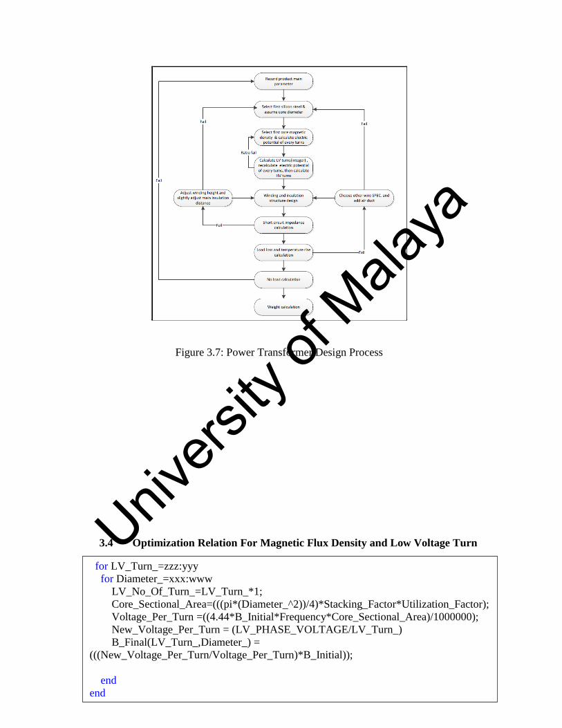
Figure 3.7: Power Transformer Design Process
3.4 Optimization Relation For Magnetic Flux Density and Low Voltage Turn
for LV_Turn_=zzz:yyy
for Diameter_=xxx:www
LV_No_Of_Turn_=LV_Turn_*1;
Core_Sectional_Area=(((pi*(Diameter_^2))/4)*Stacking_Factor*Utilization_Factor);
Voltage_Per_Turn =((4.44*B_Initial*Frequency*Core_Sectional_Area)/1000000);
New_Voltage_Per_Turn = (LV_PHASE_VOLTAGE/LV_Turn_)
B_Final(LV_Turn_,Diameter_) =
(((New_Voltage_Per_Turn/Voltage_Per_Turn)*B_Initial));
end
end
Univers
ity of
Mala
ya

32
Figure 3.8: Optimization code for the Magnetic Flux Density and Low Voltage Number
of Turn
This program lines perform nested loops based on the prompted values by the
Transformer designer. The function check first to make sure that the Core Diameter loops
based on the range prompted by the designer. It is followed by the parentheses containing
the column assigned to it. The values computed will be stored in matrices array and
indexed according to its row and column element.
3.5 Pseudo Code for the Overall Optimization Algorithm
Figure 3.9: Simplified Pseudo Code for Overall Optimization Algorithm
The data will be based on the value of the final flux density calculated from the formula
below:
𝐵𝐹𝑖𝑛𝑎𝑙 =𝐸𝑝 ′
𝐸𝑝𝑥 𝐵𝐼𝑛𝑖𝑡𝑖𝑎𝑙
Next, the constraint were set for the algorithm to search for the optimized value. Here, the
value required is as below condition:
𝐵𝐹𝑖𝑛𝑎𝑙 ≈ 𝐵𝐼𝑛𝑖𝑡𝑖𝑎𝑙
data = B_Final;
[minNumCol, minIndexCol] = (min(abs(data-B_Initial)));
[maxNum, Core_Diameter] = min(minNumCol);
LV_Turn_Optimized = minIndexCol(Core_Diameter);
(44)
(45)
Univers
ity of
Mala
ya

33
Where the value of the 𝐵𝐹𝑖𝑛𝑎𝑙 is set to be as close to as the 𝐵𝐼𝑛𝑖𝑡𝑖𝑎𝑙 values in this
design case is at 1.7 Tesla.
This function sorts the structure based on the 𝐵𝐹𝑖𝑛𝑎𝑙 values. The function check first to
make sure that the Core Diameter loops based on the range prompted by the designer. It
is followed by the parentheses containing the column assigned to it and at the same time
identifying the optimized Low Voltage number of turn committed to it. In order to
achieve the minimum power loss, the Medium Frequency Transformer should operate at
the optimum flux density which can be calculated by the equation [17].Using this
combined function, the elements of the row and column are compared to determine the
optimized value [18].
CHAPTER 4
RESULT OF POWER TRANSFORMER DESIGN OPTIMIZATION
4.1 Introduction
Univers
ity of
Mala
ya

34
In this chapter, the results of this study are explained and going to be discussed. For this
purpose, the results are focused on the Core Diameter values, Number of Low Voltage
Turns, Percentage of Resistance, Reactance and Impedance as well as the No Load
Losses. In order to determine the optimized design of the Power Transformer based on
the mentioned important and high performance parameters, section 4.2 shows the results
of a preliminary result of a Conventional Calculation Method (CCM) Power Transformer
design. Section 4.3 shows the result of the Power Transformer after optimization. There
are few curves obtained in giving justification ot the optimized design using Nested
Loop. In Section 4.4, both the results from Conventional Calculation Method (CCM) and
Nested Loop are compared to determine which method is able to give better optimized
Power Transformer design.
4.2 Conventional Calculation Method (CCM) of Power Transformer Design
The Conventional Calculation Method (CCM) Power Transformer Design is designing
through trial and error method. The typical medium rating Power Transformer
specification are as Table 4.1. The important design Parameters are tabulated in Table
4.2. The method given is used for the design calculation of Transformer which in the
opinion based on the experience in the Transformer industry, is the most realistic and
complete conventional design method available in the literature to the best of our
knowledge [19].
Rating 3-Phase, 45MVA, 132/33/11kV
Vector Group YNyn0d11
Frequency 50 Hz
Magnetic Flux Density, BINITIAL 1.7 Tesla
Impedance 10% – 20%
No Load Loss 20,000 – 25,000 Watt
Univers
ity of
Mala
ya

35
Load Loss 200,000 – 250,000 Watt
Table 4.1: Conventional Calculation Method (CCM) Design Parameters
Core Diameter, D 650mm
Number of Low Voltage Turn, LV Turn 166 Turn
Induced Voltage, 𝐸𝑝 114.774
Voltage Per Turn, 𝐸𝑝 ′ 115.383
Magnetic Flux Density, BFINAL 1.69104
Table 4.2: Conventional Calculation Method (CCM) Design Parameters
Design Variable Result
MINIMUM NOMINAL MAXIMUM
Core Weight, (kg) 26581.7
Reactance Percentage, % X 13.0894 13.7125 14.2932
Resistance Percentage, % R 0.48936 0.39801 0.396184
Impedance Percentage, % Z 13.0985 13.7183 14.2987
No Load Loss, NLL (Watt) 23817.2
Load Loss, LL (Watt) 220212 179106 178283
Table 4.3: Conventional Calculation Method (CCM) Electrical Performance
By using the design parameters and the assumptions made in section 3.2, the Electrical
Performance as shown in Table 4.2 can be achieved. The data shows that with current
core diameter of 650mm as per Table 4.1, the weight of core is 26581.7 kg. The cost is
assumed to be directly proportional to the weight of the core. It is also found that the
Univers
ity of
Mala
ya
36
Impedance value were kept at 13% to 14% value. The total Losses were calculated
between 178kW to 220kW.
Based on the computed result, the Power Transformer is fit for production and
manufacturing process. The electrical performance were considered standard as per
current market, However, from the eye of a Sales and Marketing executives and potential
customer, the costing is considered high, there is always a way to fulfill the cost saving
while keeping the electrical performance optimization on par. This is where the research
and development begin and the conventional calculation method (CCM) will be
transform to optimized design.
4.3 Nested Loop Optimization of Power Transformer Design
In Nested Loop optimization, the initial dimension of the Core Diameter, (D), Magnetic
Flux Density (BFINAL), Induced Voltage (Ep), Voltage per Turn (Ep‟) and the number of
Turn (LV Turn) are determined by the algorithm instead of trial and error mode. The initial
values of optimization were prompted by the Transformer Designer during the
optimization process.
Univers
ity of
Mala
ya

37
Figure 4.1: Prompt Data Pop-Up for Optimization Criterion
Figure 4.2: Prompt Data Acquisition for Optimization Criterion of Core Diameter Univers
ity of
Mala
ya
38
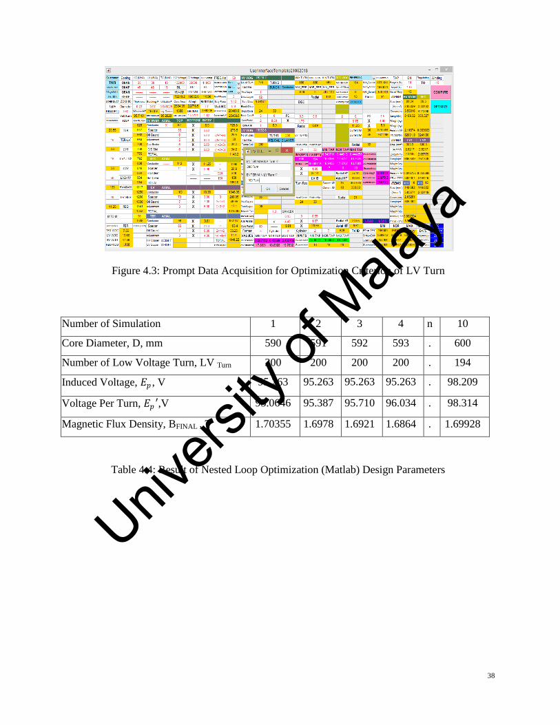
Figure 4.3: Prompt Data Acquisition for Optimization Criterion of LV Turn
Number of Simulation 1 2 3 4 n 10
Core Diameter, D, mm 590 591 592 593 . 600
Number of Low Voltage Turn, LV Turn 200 200 200 200 . 194
Induced Voltage, 𝐸𝑝 , V 95.263 95.263 95.263 95.263 . 98.209
Voltage Per Turn, 𝐸𝑝 ′,V 95.0646 95.387 95.710 96.034 . 98.314
Magnetic Flux Density, BFINAL , T 1.70355 1.6978 1.6921 1.6864 . 1.69928
Table 4.4: Result of Nested Loop Optimization (Matlab) Design Parameters
Univers
ity of
Mala
ya

39
Design Variable Result
MINIMUM NOMINAL MAXIMUM
Core Weight, (kg) 23414.2
Reactance Percentage, % X 16.9396 17.8731 18.7028
Resistance Percentage, % R 0.549711 0.44613 0.444258
Impedance Percentage, % Z 16.9485 17.8787 18.7081
No Load Loss, NLL (Watt) 20979.2
Load Loss, LL (Watt) 247370 200758 199916
Table 4.5: Result of Nested Loop Optimization Electrical Performance (Ø = 600mm)
Figure 4.4: Convergence Characteristic of Nested Loop Optimization
The optimization will commenced with acquisition of input from designer. A range of
Core Diameter dimension will be prompted as well as the Low Voltage number of turn
range. For this example the range of the Core dimension is between 590mm to 600mm
while for Low Voltage number of turn in between 200 to 100 turn. In this study, the
optimized criterion chosen was the Core Diameter in order to reduce the dimension of the
Core. The data shows that the optimized core diameter can be reduce up to 600mm as per
Table 4.3, and the weight of core is reduced to 23414.2 kg respectively. The cost will be
Univers
ity of
Mala
ya

40
shrinking as a result of the optimization. On the other side of the electrical performances,
it is also found that the Impedance value were increasing from 16% to 18%. The total
Losses were calculated between 204kW to 255kW.
4.4 Result Comparison between CCM (Conventional Calculation Method) and
Nested Loop Optimization
In this section, both of the result from Conventional Calculation Method (CCM) and
Nested Loop Optimization are compared. The comparison is made by comparing the
dimension of the Core Diameter, Number of Low Voltage Turn (LV Turn), Magnetic Flux
Density (B FiTal), Electrical performance and also the Transformer Core Weight. The
comparison result is tabulated in Table 4.5.
Design Parameters Designing Method
Conventional
Calculation Method
(CCM)
Nested Loop
Optimization
(Matlab)
Core Diameter, D 650mm 600mm
Number of Low Voltage Turn, LV
Turn
166 Turn 194 Turn
Induced Voltage, 𝐸𝑝 114.774 98.209
Voltage Per Turn, 𝐸𝑝 ′ 115.383 98.314
Magnetic Flux Density, BFINAL 1.69104 1.69928
Table 4.6: Result of Comparison between CCM and Nested Loop Optimization
Univers
ity of
Mala
ya

41
Design
Variable
Conventional Calculation Method
(CCM)
Nested Loop Optimization (Matlab)
MINIMUM NOMINAL MAXIMUM MINIMUM NOMINAL MAXIMUM
Core
Weight,
(kg)
26581.7 23414.2
Reactance
Percentage,
% X
13.0894 13.7125 14.2932 16.9396 17.8731 18.7028
Resistance
Percentage,
% R
0.48936 0.39801 0.396184 0.549711 0.44613 0.444258
Impedance
Percentage,
% Z
13.0985 13.7183 14.2987 16.9485 17.8787 18.7081
No Load
Loss, NLL
(Watt)
23817.2 20979.2
Load Loss,
LL (Watt)
220212 179106 178283 247370 200758 199916
Table 4.7: Result of Comparison between CCM and Nested Loop Optimization Electrical
Performance
From the result in the table 4.5 and 4.6, the optimized Core Diameter, 600mm and Low
Voltage number of turn, 194 turn were presented respectively. The voltage per turn and
Magnetic Flux density were 98.314 and 1.69928 respectively. It is observed that the Core
Diameter can be reduced up to 7% as a result of the optimization technique of the Nested
Loop. Consequently, with the 7% reduction of the Core Diameter, the weight of the core
will follow through with reduction up to 11.9%. The No-Load Loss also will see further
Univers
ity of
Mala
ya

42
reduction also up to 11.9%. From a manufacturing side of view, the reduction in the
Core Weight is significant due to the amount of raw materials and handling involved. The
positive reduction also will give back to the spoilage during manufacturing process if
considered the total mass production events. To the Sales and Marketing executives, this
will be a positives sales margin keeping the same selling price tag but with a lower
overhead cost. However, for every manufacturing design, there are always a trade-off.
The optimization using nested loop will yield a higher total Load Loss. This is due to for
every inches of dimension reduction on the Core Diameter, the number of Low Voltage
Turn will be increased. Hence, the length of Copper will be increased and resulting for a
higher Impedance value and I2R Load Loss. In this case, a potential customer will be
advised on the specification and tolerable values of the Transformer to be installed to the
Grid system with agreement on both parties involved.
Univers
ity of
Mala
ya

43
CHAPTER 5
CONSLUSION AND FUTURE WORKS
5.1 Conclusion
In this work, optimization of the Conventional Calculation Method (CCM) of the Power
Transformer design has been successfully performed. One main algorithms were used in
this study namely Nested Loop Optimization (MATLAB). The conventional calculation
method still uses the Excel sheet as part of trial and error method in designing Power
Transformer whereas the Nested Loop Optimization were using sophisticated user GUI
technique developed in the MATLAB software environment. The electrical performance
was evaluated based on the Core Diameter dimension, number of Low Voltage turn (LV
Turn), No-Load Loss, Core Weight and also the total Load Losses.
From the result that has been obtained, Nested Loop Optimization yield the optimum
result in terms of cost saving and practicality over the Conventional Calculation Method
(CCM). Furthermore, the time consuming when using the Conventional Calculation
Method (CCM) in excel sheets can be phase out with the application style of the Designer
GUI at the fingertip just to give broad ideas and consideration on the designing
parameters and optimization.
Univers
ity of
Mala
ya

44
5.2 Future Work
Future work that can be performed are as follows:-
1. A hybrid algorithm can be proposed. Few other function optimization algorithm
can be used namely Genetic Algorithm (GA), Particle Swarm Optimization (PSO)
and Back Search Algorithm (BSA) for the Power Transformer Design
Optimization.
2. Use more parameters as variable for optimization of the Power Transformer
3. Develop an application tools of designing and optimization coupled together for
android environment. This to be in line with the upcoming revolution of Industrial
4.0.
Univers
ity of
Mala
ya

45
REFERENCES
[1] H. M. O. R. Ajay Khatri, "Optimal Design of Power Transformer using
Genetic Algorithm," 2012 International Conference on Communication
System and Network Technologies, vol. I, no. I, p. 3, 2012.
[2] A. Rubaai, "Computer Aided Instruction of Power Transformer Design in the
Undergraduate Power Engineering Class," IEEE Transaction on Power
System, vol. 9, no. 3, p. 7, 1994.
[3] C. D. C. S. A. T. T. H. K. B. Sriram Vaisambhayana, "State of Art Survey
for design of Medium Frequency High Power Transformer," IEEE, vol. 1,
no. 1, p. 9, 2016.
[4] S. T. A. R. Abdul Razak, "Design Consideration of A High Frequency Power
Transformer," in National Power and Energy Conference (PECon) 2003
Proceedings, Bangi, Malaysia, Selangor, Malaysia, 2003.
[5] T. L. Christian Freitag, "Mixed Core Design For Power Transformer To
Reduce Core Losses," IEEE, Vols. 978-1-5090-4489-4, no. 17, p. 1, 2017.
[6] D. Houcque, Introduction to MATLAB for Engineering Students, Evanston,
Illinois: McCormick School of Engineering and Applied Science, 2005.
[7] S. Attaway, Matlab A Practical Approach, Boston, MA: Elsevier Inc., 2009.
[8] A. Gilat, MATLAB An Introduction With Appliaction, Ohio: John Wiley &
Sons Inc., 2011.
[9] S. K. S.V Kulkarni, Transformer Engineering Design And Practice, Mumbai:
Marcel Dekker Inc., 2004.
[10] A. G. B. U. V. I. E. O. A. R. Irma Villar, "Proposal And Validation Of
Univers
ity of
Mala
ya

46
Medium Frequency Power Transformer Design Methodology," IEEE, Vols.
978-1-4577-0541-0, no. 11, p. 2, 2011.
[11] P. S. B. Simon C. Bell, "Power Transformer Design using Magnetic Circuit
Theory and Finite Element Analysis-A Comparison of Technique," IEEE,
vol. 1, no. 1, p. 6, 2004.
[12] B. S. R. F. M. P. S. L. P. B. D. P. El Nahas, "Three Dimensional Flux
Calculation On A Three-Phase Transformer," IEEE, Vols. 85 SM 378-5, no.
1, pp. 156-160, 1986.
[13] L. H. G. P. O. C. S A Holland, "A Power Transformer Design With Finite
Elements - A Company Experience," IEEE, vol. 1, no. 1, p. 3, 1991.
[14] S. P. Robert J. Carcoran, "Mechanical Properties Of Copper In Relation To
Power Transformer Design," Power Engineering Journal, vol. 1, no. 1, p. 1,
1987.
[15] Z. G. L. K. L. T. L. S. F. Y. W. B. Niu When Hao, "Development and
Application Of Automatic Software Based On APDL For Optimizing
Insulation Design Of Power Transformer," IEEE, Vols. 978-1-5090-0496-
6/16, no. 16, p. 2, 2016.
[16] H. E. C. Ltd., "Electromagnetic Design Manual Cast Resin 3D Wound Core
Dry Type Transformer Technical License Project". China 01 January 2015.
[17] T. I. J. C. B. Cheng Deng, "Design Of Medim Frequency Transformer With
Silicon Steel For Mobile Power Substation," IEEE Transaction, Vols. 978-1-
5090-1/17, no. 1, p. 3, 2017.
[18] Jan, "MATLAB ANSWER," MATLAB, MONDAY JULY 2018. [Online].
Available: https://jp.mathworks.com/matlabcentral/answers/3221-finding-
the-row-and-column-number-in-a-matrix. [Accessed 01 JULY 2018].
Univers
ity of
Mala
ya

47
[19] N. Y. Levent Alhan, "Discrete Design Optimization Of Distribution
Transformer With Guaranteed Optimum Convergence Using Cuckoo Search
Algorithm," Turkish Journal of Electrical Engineering And Computer
Sciences, vol. 1, no. 1, p. 5, 2017.
Univers
ity of
Mala
ya