LABORATORY OF COMPUTER PROGRAMMING

R: COLLECTION OF EXERCISES

FILIPPO PICCININI University of Bologna f.piccinini@unibo.it

DESCRIPTION This is a collection of exercises useful to learn how to use the basic data types of R. Additionally, a very interesting website full of useful exercises on the basic features of R is: https://www.w3resource.com/r-programming-exercises/

SOURCE: https://www.r-exercises.com/2019/08/05/working-with-vectors/

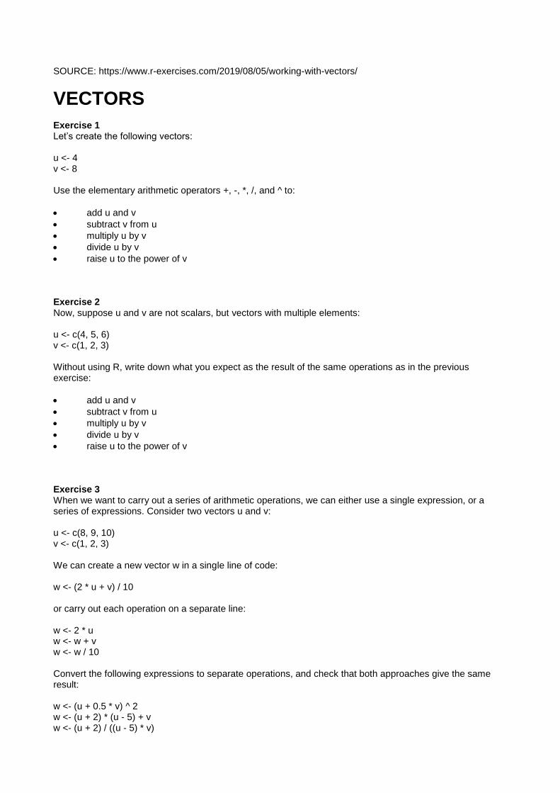
VECTORS Exercise 1 Let’s create the following vectors: u <- 4 v <- 8 Use the elementary arithmetic operators +, -, *, /, and ^ to:

add u and v

subtract v from u

multiply u by v

divide u by v

raise u to the power of v Exercise 2 Now, suppose u and v are not scalars, but vectors with multiple elements: u <- c(4, 5, 6) v <- c(1, 2, 3) Without using R, write down what you expect as the result of the same operations as in the previous exercise:

add u and v

subtract v from u

multiply u by v

divide u by v

raise u to the power of v Exercise 3 When we want to carry out a series of arithmetic operations, we can either use a single expression, or a series of expressions. Consider two vectors u and v: u <- c(8, 9, 10) v <- c(1, 2, 3) We can create a new vector w in a single line of code: w <- (2 * u + v) / 10 or carry out each operation on a separate line: w <- 2 * u w <- w + v w <- w / 10 Convert the following expressions to separate operations, and check that both approaches give the same result: w <- (u + 0.5 * v) ^ 2 w <- (u + 2) * (u - 5) + v w <- (u + 2) / ((u - 5) * v)

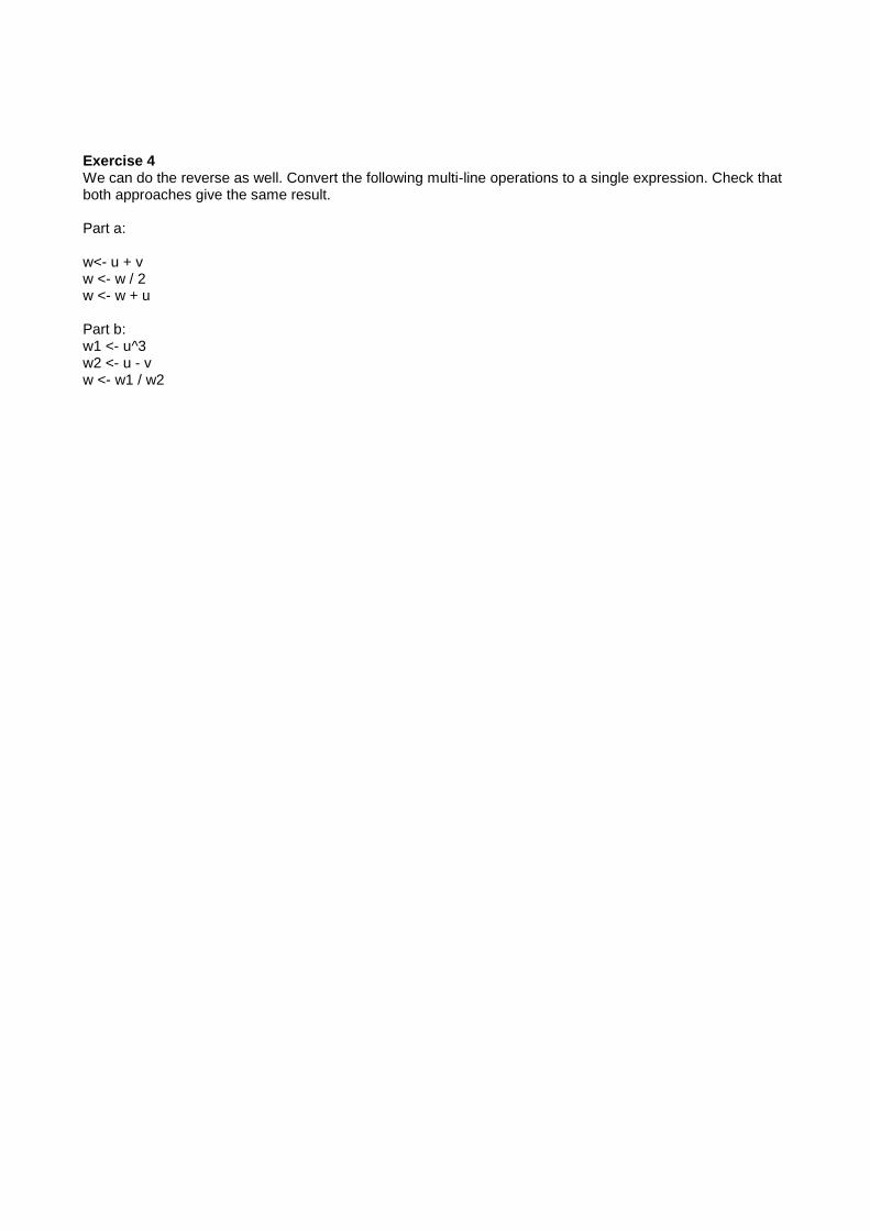
Exercise 4 We can do the reverse as well. Convert the following multi-line operations to a single expression. Check that both approaches give the same result. Part a: w<- u + v w <- w / 2 w <- w + u Part b: w1 <- u^3 w2 <- u - v w <- w1 / w2

SOURCE: https://www.r-exercises.com/2019/08/05/working-with-vectors/

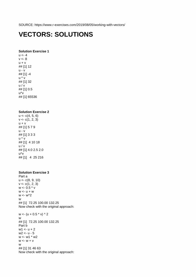
VECTORS: SOLUTIONS Solution Exercise 1 u <- 4 v <- 8 u + v ## [1] 12 u - v ## [1] -4 u * v ## [1] 32 u / v ## [1] 0.5 u^v ## [1] 65536 Solution Exercise 2 u <- c(4, 5, 6) v <- c(1, 2, 3) u + v ## [1] 5 7 9 u - v ## [1] 3 3 3 u * v ## [1] 4 10 18 u / v ## [1] 4.0 2.5 2.0 u^v ## [1] 4 25 216 Solution Exercise 3 Part a u <- c(8, 9, 10) v <- c(1, 2, 3) w <- 0.5 * v w <- u + w w <- w^2 w ## [1] 72.25 100.00 132.25 Now check with the original approach: w <- (u + 0.5 * v) ^ 2 w ## [1] 72.25 100.00 132.25 Part b w1 <- u + 2 w2 <- u - 5 w <- w1 * w2 w <- w + v w ## [1] 31 46 63 Now check with the original approach:

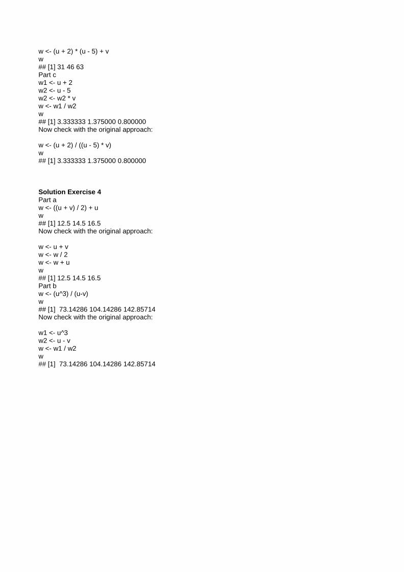
w <- (u + 2) * (u - 5) + v w ## [1] 31 46 63 Part c w1 <- u + 2 w2 <- u - 5 w2 <- w2 * v w <- w1 / w2 w ## [1] 3.333333 1.375000 0.800000 Now check with the original approach: w <- (u + 2) / ((u - 5) * v) w ## [1] 3.333333 1.375000 0.800000 Solution Exercise 4 Part a w <- ((u + v) / 2) + u w ## [1] 12.5 14.5 16.5 Now check with the original approach: w <- u + v w <- w / 2 w <- w + u w ## [1] 12.5 14.5 16.5 Part b w <- (u^3) / (u-v) w ## [1] 73.14286 104.14286 142.85714 Now check with the original approach: w1 <- u^3 w2 <- u - v w <- w1 / w2 w ## [1] 73.14286 104.14286 142.85714

SOURCE: https://www.r-bloggers.com/data-frame-exercises/

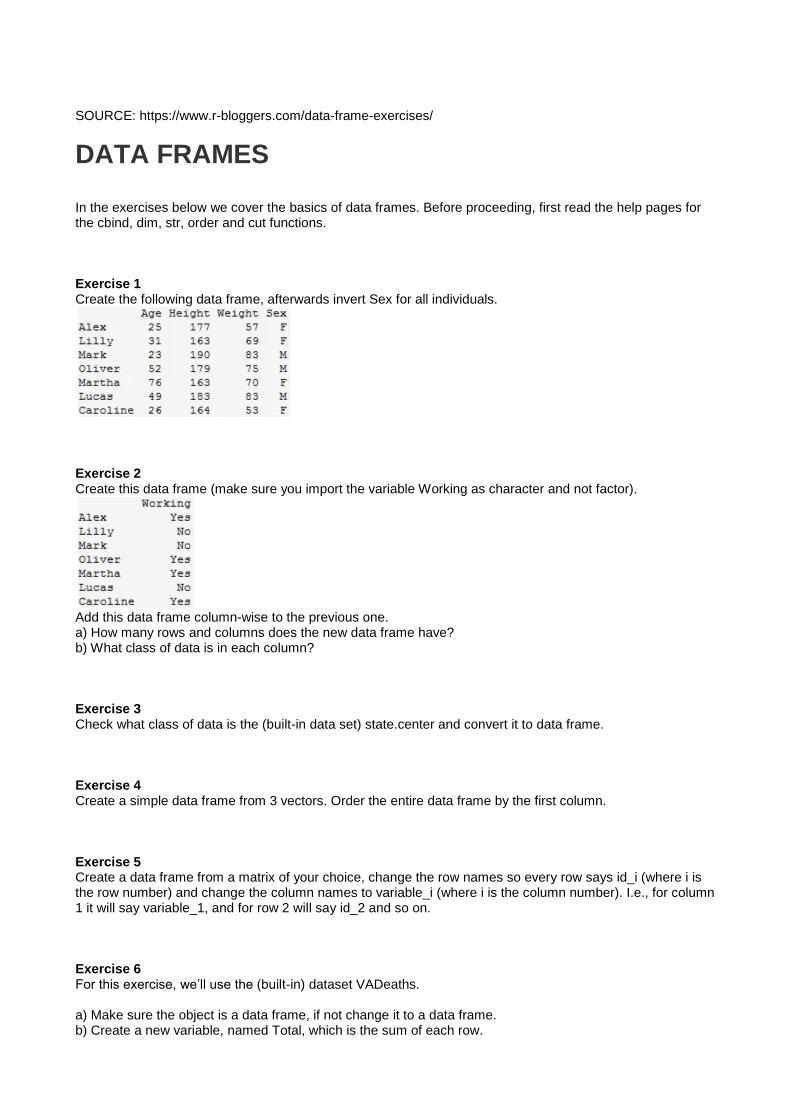
DATA FRAMES In the exercises below we cover the basics of data frames. Before proceeding, first read the help pages for the cbind, dim, str, order and cut functions. Exercise 1 Create the following data frame, afterwards invert Sex for all individuals.

Exercise 2 Create this data frame (make sure you import the variable Working as character and not factor).

Add this data frame column-wise to the previous one. a) How many rows and columns does the new data frame have? b) What class of data is in each column? Exercise 3 Check what class of data is the (built-in data set) state.center and convert it to data frame. Exercise 4 Create a simple data frame from 3 vectors. Order the entire data frame by the first column. Exercise 5 Create a data frame from a matrix of your choice, change the row names so every row says id_i (where i is the row number) and change the column names to variable_i (where i is the column number). I.e., for column 1 it will say variable_1, and for row 2 will say id_2 and so on. Exercise 6 For this exercise, we’ll use the (built-in) dataset VADeaths. a) Make sure the object is a data frame, if not change it to a data frame. b) Create a new variable, named Total, which is the sum of each row.

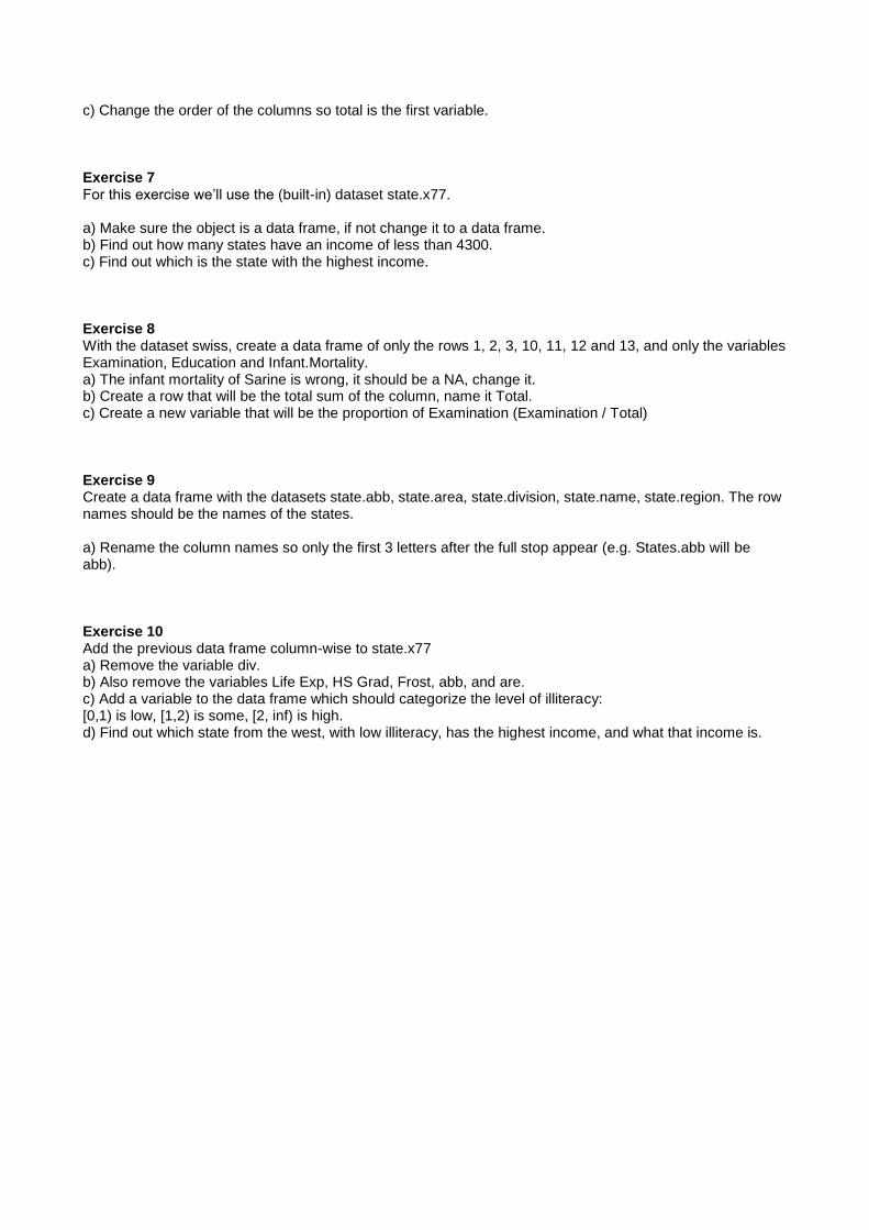
c) Change the order of the columns so total is the first variable. Exercise 7 For this exercise we’ll use the (built-in) dataset state.x77. a) Make sure the object is a data frame, if not change it to a data frame. b) Find out how many states have an income of less than 4300. c) Find out which is the state with the highest income. Exercise 8 With the dataset swiss, create a data frame of only the rows 1, 2, 3, 10, 11, 12 and 13, and only the variables Examination, Education and Infant.Mortality. a) The infant mortality of Sarine is wrong, it should be a NA, change it. b) Create a row that will be the total sum of the column, name it Total. c) Create a new variable that will be the proportion of Examination (Examination / Total) Exercise 9 Create a data frame with the datasets state.abb, state.area, state.division, state.name, state.region. The row names should be the names of the states. a) Rename the column names so only the first 3 letters after the full stop appear (e.g. States.abb will be abb). Exercise 10 Add the previous data frame column-wise to state.x77 a) Remove the variable div. b) Also remove the variables Life Exp, HS Grad, Frost, abb, and are. c) Add a variable to the data frame which should categorize the level of illiteracy: [0,1) is low, [1,2) is some, [2, inf) is high. d) Find out which state from the west, with low illiteracy, has the highest income, and what that income is.

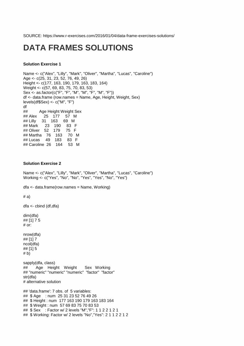
SOURCE: https://www.r-exercises.com/2016/01/04/data-frame-exercises-solutions/

DATA FRAMES SOLUTIONS Solution Exercise 1 Name <- c("Alex", "Lilly", "Mark", "Oliver", "Martha", "Lucas", "Caroline") Age <- c(25, 31, 23, 52, 76, 49, 26) Height <- c(177, 163, 190, 179, 163, 183, 164) Weight <- c(57, 69, 83, 75, 70, 83, 53) Sex <- as.factor(c("F", "F", "M", "M", "F", "M", "F")) df <- data.frame (row.names = Name, Age, Height, Weight, Sex) levels(df$Sex) <- c("M", "F") df ## Age Height Weight Sex ## Alex 25 177 57 M ## Lilly 31 163 69 M ## Mark 23 190 83 F ## Oliver 52 179 75 F ## Martha 76 163 70 M ## Lucas 49 183 83 F ## Caroline 26 164 53 M Solution Exercise 2 Name <- c("Alex", "Lilly", "Mark", "Oliver", "Martha", "Lucas", "Caroline") Working <- c("Yes", "No", "No", "Yes", "Yes", "No", "Yes") dfa <- data.frame(row.names = Name, Working) # a) dfa <- cbind (df,dfa) dim(dfa) ## [1] 7 5 # or: nrow(dfa) ## [1] 7 ncol(dfa) ## [1] 5 # b) sapply(dfa, class) ## Age Height Weight Sex Working ## "numeric" "numeric" "numeric" "factor" "factor" str(dfa) # alternative solution ## 'data.frame': 7 obs. of 5 variables: ## $ Age : num 25 31 23 52 76 49 26 ## $ Height : num 177 163 190 179 163 183 164 ## $ Weight : num 57 69 83 75 70 83 53 ## $ Sex : Factor w/ 2 levels "M","F": 1 1 2 2 1 2 1 ## $ Working: Factor w/ 2 levels "No","Yes": 2 1 1 2 2 1 2

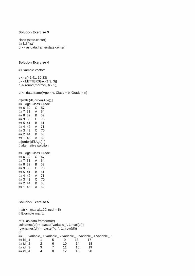
Solution Exercise 3 class (state.center) ## [1] "list" df <- as.data.frame(state.center) Solution Exercise 4 # Example vectors v <- c(45:41, 30:33) b <- LETTERS[rep(1:3, 3)] n <- round(rnorm(9, 65, 5)) df <- data.frame(Age = v, Class = b, Grade = n) df[with (df, order(Age)),] ## Age Class Grade ## 6 30 C 57 ## 7 31 A 64 ## 8 32 B 59 ## 9 33 C 73 ## 5 41 B 61 ## 4 42 A 71 ## 3 43 C 70 ## 2 44 B 63 ## 1 45 A 62 df[order(df$Age), ] # alternative solution ## Age Class Grade ## 6 30 C 57 ## 7 31 A 64 ## 8 32 B 59 ## 9 33 C 73 ## 5 41 B 61 ## 4 42 A 71 ## 3 43 C 70 ## 2 44 B 63 ## 1 45 A 62 Solution Exercise 5 matr <- matrix(1:20, ncol = 5) # Example matrix df <- as.data.frame(matr) colnames(df) <- paste("variable_", 1:ncol(df)) rownames(df) <- paste("id_", 1:nrow(df)) df ## variable_ 1 variable_ 2 variable_ 3 variable_ 4 variable_ 5 ## id_ 1 1 5 9 13 17 ## id_ 2 2 6 10 14 18 ## id_ 3 3 7 11 15 19 ## id_ 4 4 8 12 16 20

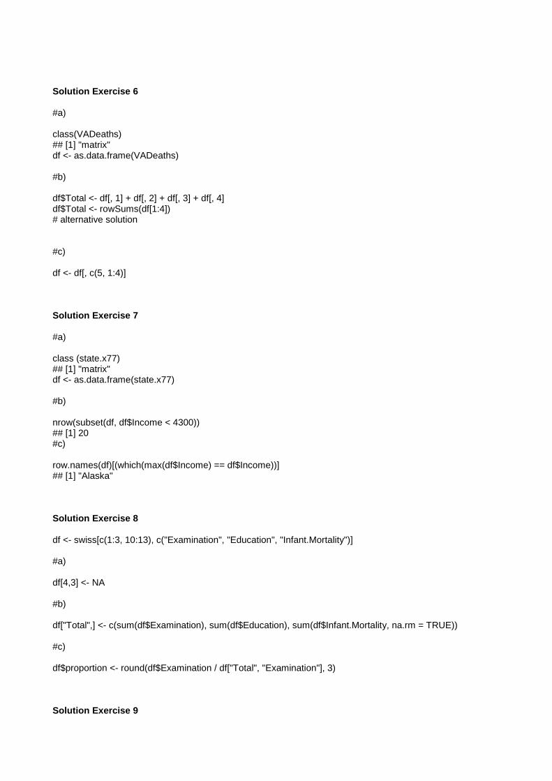
Solution Exercise 6 #a) class(VADeaths) ## [1] "matrix" df <- as.data.frame(VADeaths) #b) df$Total <- df[, 1] + df[, 2] + df[, 3] + df[, 4] df$Total <- rowSums(df[1:4]) # alternative solution #c) df <- df[, c(5, 1:4)] Solution Exercise 7 #a) class (state.x77) ## [1] "matrix" df <- as.data.frame(state.x77) #b) nrow(subset(df, df$Income < 4300)) ## [1] 20 #c) row.names(df)[(which(max(df$Income) == df$Income))] ## [1] "Alaska" Solution Exercise 8 df <- swiss[c(1:3, 10:13), c("Examination", "Education", "Infant.Mortality")] #a) df[4,3] <- NA #b) df["Total",] <- c(sum(df$Examination), sum(df$Education), sum(df$Infant.Mortality, na.rm = TRUE)) #c) df$proportion <- round(df$Examination / df["Total", "Examination"], 3) Solution Exercise 9

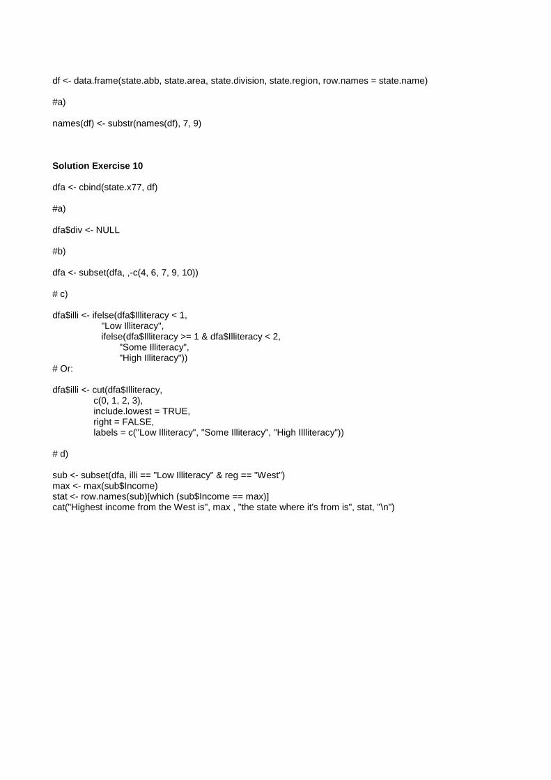
df <- data.frame(state.abb, state.area, state.division, state.region, row.names = state.name) #a) names(df) <- substr(names(df), 7, 9) Solution Exercise 10 dfa <- cbind(state.x77, df) #a) dfa$div <- NULL #b) dfa <- subset(dfa, ,-c(4, 6, 7, 9, 10)) # c) dfa$illi <- ifelse(dfa$Illiteracy < 1, "Low Illiteracy", ifelse(dfa$Illiteracy >= 1 & dfa$Illiteracy < 2, "Some Illiteracy", "High Illiteracy")) # Or: dfa$illi <- cut(dfa$Illiteracy, c(0, 1, 2, 3), include.lowest = TRUE, right = FALSE, labels = c("Low Illiteracy", "Some Illiteracy", "High Illliteracy")) # d) sub <- subset(dfa, illi == "Low Illiteracy" & reg == "West") max <- max(sub$Income) stat <- row.names(sub)[which (sub$Income == max)] cat("Highest income from the West is", max , "the state where it's from is", stat, "\n")

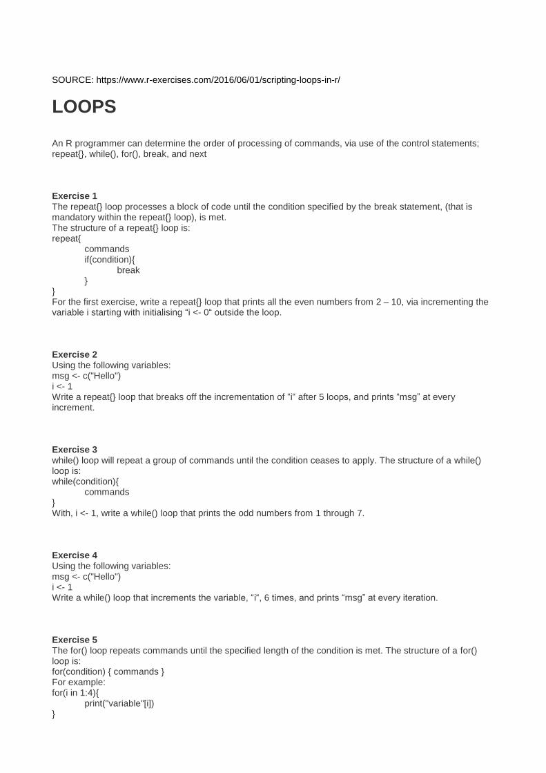
SOURCE: https://www.r-exercises.com/2016/06/01/scripting-loops-in-r/

LOOPS An R programmer can determine the order of processing of commands, via use of the control statements; repeat{}, while(), for(), break, and next Exercise 1 The repeat{} loop processes a block of code until the condition specified by the break statement, (that is mandatory within the repeat{} loop), is met. The structure of a repeat{} loop is: repeat{ commands if(condition){ break } } For the first exercise, write a repeat{} loop that prints all the even numbers from 2 – 10, via incrementing the variable i starting with initialising “i <- 0“ outside the loop. Exercise 2 Using the following variables: msg <- c("Hello") i <- 1 Write a repeat{} loop that breaks off the incrementation of “i“ after 5 loops, and prints “msg” at every increment. Exercise 3 while() loop will repeat a group of commands until the condition ceases to apply. The structure of a while() loop is: while(condition){ commands } With, i <- 1, write a while() loop that prints the odd numbers from 1 through 7. Exercise 4 Using the following variables: msg <- c("Hello") i <- 1 Write a while() loop that increments the variable, “i“, 6 times, and prints “msg” at every iteration. Exercise 5 The for() loop repeats commands until the specified length of the condition is met. The structure of a for() loop is: for(condition) { commands } For example: for(i in 1:4){ print("variable"[i]) }

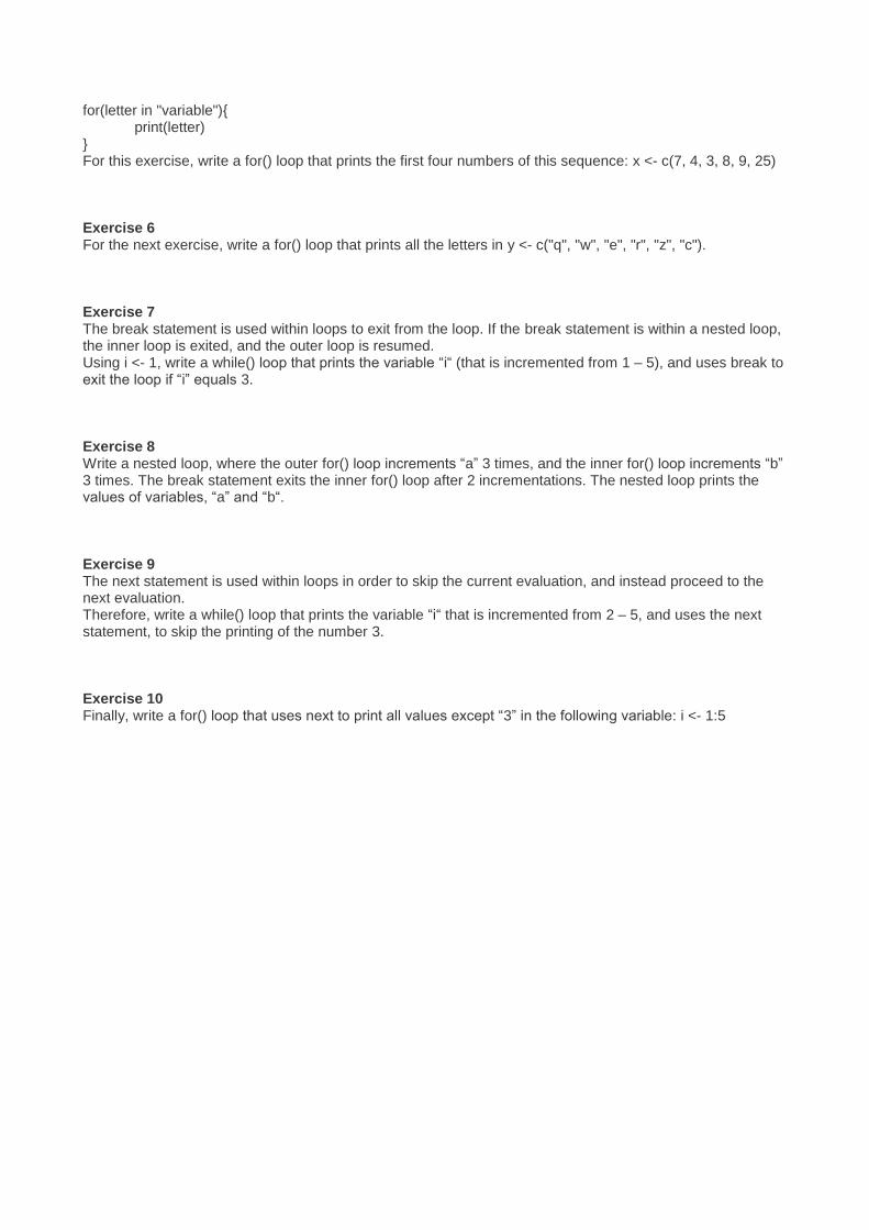
for(letter in "variable"){ print(letter) } For this exercise, write a for() loop that prints the first four numbers of this sequence: x <- c(7, 4, 3, 8, 9, 25) Exercise 6 For the next exercise, write a for() loop that prints all the letters in y <- c("q", "w", "e", "r", "z", "c"). Exercise 7 The break statement is used within loops to exit from the loop. If the break statement is within a nested loop, the inner loop is exited, and the outer loop is resumed. Using i <- 1, write a while() loop that prints the variable “i“ (that is incremented from 1 – 5), and uses break to exit the loop if “i” equals 3. Exercise 8 Write a nested loop, where the outer for() loop increments “a” 3 times, and the inner for() loop increments “b” 3 times. The break statement exits the inner for() loop after 2 incrementations. The nested loop prints the values of variables, “a” and “b“. Exercise 9 The next statement is used within loops in order to skip the current evaluation, and instead proceed to the next evaluation. Therefore, write a while() loop that prints the variable “i“ that is incremented from 2 – 5, and uses the next statement, to skip the printing of the number 3. Exercise 10 Finally, write a for() loop that uses next to print all values except “3” in the following variable: i <- 1:5

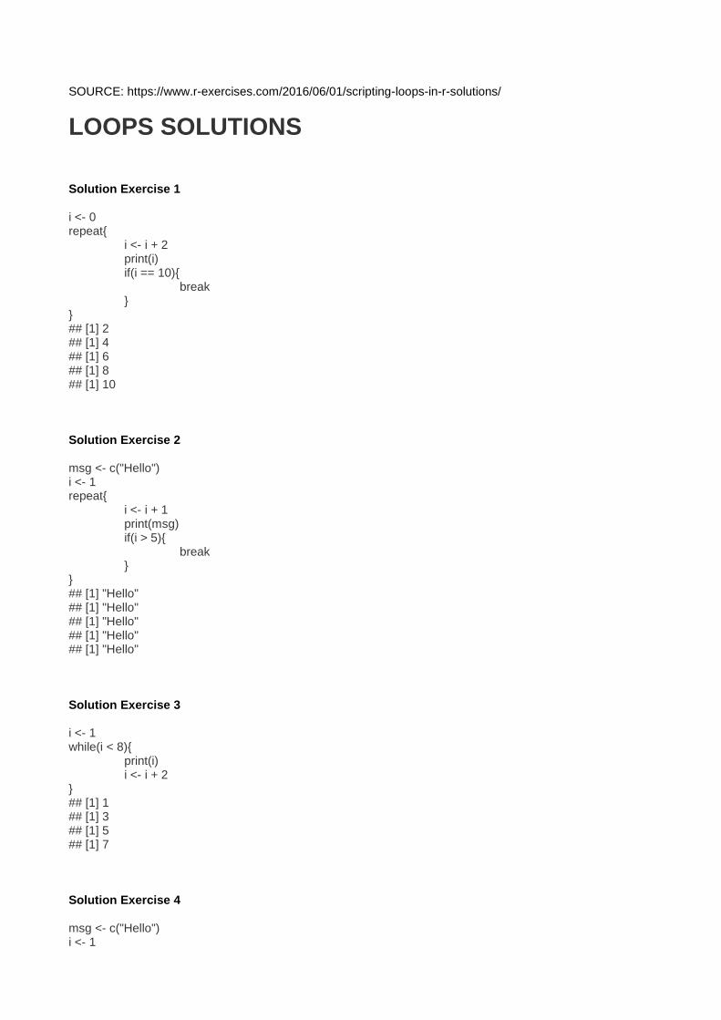
SOURCE: https://www.r-exercises.com/2016/06/01/scripting-loops-in-r-solutions/

LOOPS SOLUTIONS Solution Exercise 1 i <- 0 repeat{ i <- i + 2 print(i) if(i == 10){ break } } ## [1] 2 ## [1] 4 ## [1] 6 ## [1] 8 ## [1] 10 Solution Exercise 2 msg <- c("Hello") i <- 1 repeat{ i <- i + 1 print(msg) if(i > 5){ break } } ## [1] "Hello" ## [1] "Hello" ## [1] "Hello" ## [1] "Hello" ## [1] "Hello" Solution Exercise 3 i <- 1 while(i < 8){ print(i) i <- i + 2 } ## [1] 1 ## [1] 3 ## [1] 5 ## [1] 7 Solution Exercise 4 msg <- c("Hello") i <- 1

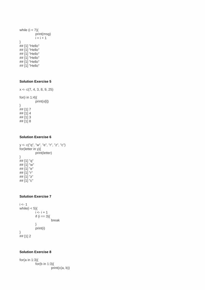
while (i < 7){ print(msg) i = i + 1 } ## [1] "Hello" ## [1] "Hello" ## [1] "Hello" ## [1] "Hello" ## [1] "Hello" ## [1] "Hello" Solution Exercise 5 x <- c(7, 4, 3, 8, 9, 25) for(i in 1:4){ print(x[i]) } ## [1] 7 ## [1] 4 ## [1] 3 ## [1] 8 Solution Exercise 6 y <- c("q", "w", "e", "r", "z", "c") for(letter in y){ print(letter) } ## [1] "q" ## [1] "w" ## [1] "e" ## [1] "r" ## [1] "z" ## [1] "c" Solution Exercise 7 i <- 1 while(i < 5){ i <- i + 1 if (i == 3){ break } print(i) } ## [1] 2 Solution Exercise 8 for(a in 1:3){ for(b in 1:3){ print(c(a, b))

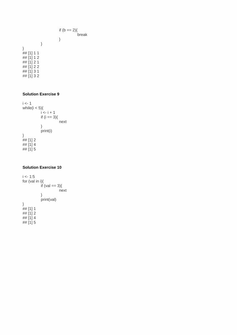
if (b == 2){ break } } } ## [1] 1 1 ## [1] 1 2 ## [1] 2 1 ## [1] 2 2 ## [1] 3 1 ## [1] 3 2 Solution Exercise 9 i <- 1 while(i < 5){ i <- i + 1 if (i == 3){ next } print(i) } ## [1] 2 ## [1] 4 ## [1] 5 Solution Exercise 10 i <- 1:5 for (val in i){ if (val == 3){ next } print(val) } ## [1] 1 ## [1] 2 ## [1] 4 ## [1] 5

SOURCE: https://www.r-exercises.com/2016/02/07/functions-exercises/

FUNCTIONS Today we’re practicing functions! In the exercises below, you’re asked to write short R scripts that define functions aimed at specific tasks. The exercises start at an easy level, and gradually move towards slightly more complex functions. Note: For some exercises, the solution will be quite easy if you make clever use of some of R’s built-in functions. For some exercises, you might want to create a vectorized solution (i.e., avoiding loops), and/or a (usually slower) non-vectorized solution. However, the exercises do not aim to practise vectorization and speed, but rather defining and calling functions. Exercise 1 Create a function that will return the sum of 2 integers. Exercise 2 Create a function what will return TRUE if a given integer is inside a vector. Exercise 3 Create a function that given a data frame will print by screen the name of the column and the class of data it contains (e.g. Variable1 is Numeric). Exercise 4 Create the function unique, which given a vector will return a new vector with the elements of the first vector with duplicated elements removed. Exercise 5 Create a function that given a vector and an integer will return how many times the integer appears inside the vector. Exercise 6 Create a function that given a vector will print by screen the mean and the standard deviation, it will optionally also print the median. Exercise 7 Create a function that given an integer will calculate how many divisors it has (other than 1 and itself). Make the divisors appear by screen. Exercise 8 Create a function that given a data frame, and a number or character will return the data frame with the character or number changed to NA.

SOURCE: https://www.r-exercises.com/2016/02/07/functions-exercises-solutions/

FUNCTIONS SOLUTIONS Solution Exercise 1 f.sum <- function(x, y){ r <- x + y r } f.sum(5, 10) ## [1] 15 Solution Exercise 2 f.exists <- function(v, x){ exist <- FALSE i <- 1 while (i <= length(v) & !exist){ if (v[i] == x){ exist <- TRUE } i <- 1 + i } exist } f.exists(c(1:10), 10) ## [1] TRUE f.exists(c(9, 3, 1), 10) ## [1] FALSE Solution Exercise 3 f.class <- function(df){ for (i in 1:ncol(df)){ cat(names(df)[i], "is", class(df[, i]), "\n") } } f.class(cars) ## speed is numeric ## dist is numeric Solution Exercise 4 (solution A) f.uniq <- function(v){ s <- c(v[1])

for(i in 1:length(v)){ counter<-0 for(j in 1:length(s)){ if(v[i]==s[j]){ counter<-counter+1 } } if(counter==0){ s <- c(s, v[i]) } } s } (solution B) f.uniq <- function(v){ s <- c() for(i in 1:length(v)){ if(sum(v[i] == s) == 0){ s <- c(s, v[i]) } } s } f.uniq(c(9, 9, 1, 1, 1, 0)) ## [1] 9 1 0 Solution Exercise 5 f.count <- function(v, x){ count <- 0 for (i in 1:length(v)){ if (v[i] == x) { count <- count + 1 } } count } f.count(c(1:9, rep(10, 100)), 10) # The rep(a,b) function creates a vector by replicating the value a per b times ## [1] 100 Solution Exercise 6 desi <- function(x, med=FALSE){ mean <- round(mean(x), 1) stdv <- round(sd(x), 1) cat("Mean is:", mean, ", SD is:", stdv, "\n") if(med){ median <- median(x)

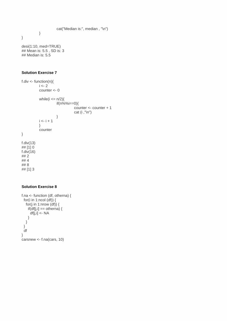
cat("Median is:", median , "\n") } } desi(1:10, med=TRUE) ## Mean is: 5.5 , SD is: 3 ## Median is: 5.5 Solution Exercise 7 f.div <- function(n){ i <- 2 counter <- 0 while(i <= n/2){ if(n%%i==0){ counter <- counter + 1 cat (i ,"\n") } i <- i + 1 } counter } f.div(13) ## [1] 0 f.div(16) ## 2 ## 4 ## 8 ## [1] 3 Solution Exercise 8 f.na <- function (df, otherna) { for(i in 1:ncol (df)) { for(j in 1:nrow (df)) { if(df[j,i] == otherna) { df[j,i] <- NA } } } df } carsnew <- f.na(cars, 10)

SOURCE: https://www.r-exercises.com/2016/01/07/reading-delimited-data/

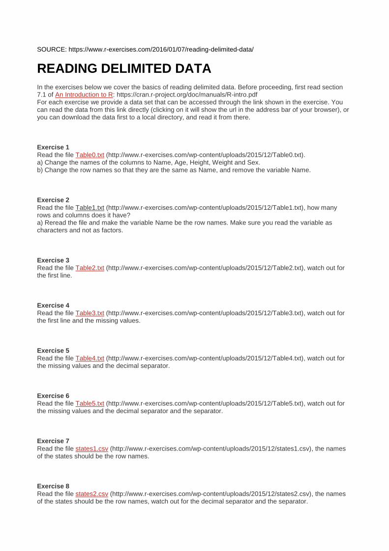
READING DELIMITED DATA In the exercises below we cover the basics of reading delimited data. Before proceeding, first read section 7.1 of An Introduction to R: https://cran.r-project.org/doc/manuals/R-intro.pdf For each exercise we provide a data set that can be accessed through the link shown in the exercise. You can read the data from this link directly (clicking on it will show the url in the address bar of your browser), or you can download the data first to a local directory, and read it from there. Exercise 1 Read the file Table0.txt (http://www.r-exercises.com/wp-content/uploads/2015/12/Table0.txt). a) Change the names of the columns to Name, Age, Height, Weight and Sex. b) Change the row names so that they are the same as Name, and remove the variable Name. Exercise 2 Read the file Table1.txt (http://www.r-exercises.com/wp-content/uploads/2015/12/Table1.txt), how many rows and columns does it have? a) Reread the file and make the variable Name be the row names. Make sure you read the variable as characters and not as factors. Exercise 3 Read the file Table2.txt (http://www.r-exercises.com/wp-content/uploads/2015/12/Table2.txt), watch out for the first line. Exercise 4 Read the file Table3.txt (http://www.r-exercises.com/wp-content/uploads/2015/12/Table3.txt), watch out for the first line and the missing values. Exercise 5 Read the file Table4.txt (http://www.r-exercises.com/wp-content/uploads/2015/12/Table4.txt), watch out for the missing values and the decimal separator. Exercise 6 Read the file Table5.txt (http://www.r-exercises.com/wp-content/uploads/2015/12/Table5.txt), watch out for the missing values and the decimal separator and the separator. Exercise 7 Read the file states1.csv (http://www.r-exercises.com/wp-content/uploads/2015/12/states1.csv), the names of the states should be the row names. Exercise 8 Read the file states2.csv (http://www.r-exercises.com/wp-content/uploads/2015/12/states2.csv), the names of the states should be the row names, watch out for the decimal separator and the separator.

SOURCE: https://www.r-exercises.com/2016/01/07/reading-delimited-data-solutions/

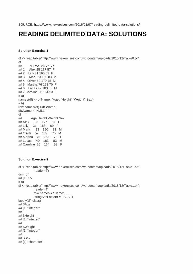
READING DELIMITED DATA: SOLUTIONS Solution Exercise 1 df <- read.table("http://www.r-exercises.com/wp-content/uploads/2015/12/Table0.txt") df ## V1 V2 V3 V4 V5 ## 1 Alex 25 177 57 F ## 2 Lilly 31 163 69 F ## 3 Mark 23 190 83 M ## 4 Oliver 52 179 75 M ## 5 Martha 76 163 70 F ## 6 Lucas 49 183 83 M ## 7 Caroline 26 164 53 F # a) names(df) <- c('Name', 'Age', 'Height', 'Weight','Sex') # b) row.names(df)<-df$Name df$Name <- NULL df ## Age Height Weight Sex ## Alex 25 177 57 F ## Lilly 31 163 69 F ## Mark 23 190 83 M ## Oliver 52 179 75 M ## Martha 76 163 70 F ## Lucas 49 183 83 M ## Caroline 26 164 53 F Solution Exercise 2 df <- read.table("http://www.r-exercises.com/wp-content/uploads/2015/12/Table1.txt", header=T) dim (df) ## [1] 7 5 # a) df <- read.table("http://www.r-exercises.com/wp-content/uploads/2015/12/Table1.txt", header=T, row.names = "Name", stringsAsFactors = FALSE) lapply(df, class) ## $Age ## [1] "integer" ## ## $Height ## [1] "integer" ## ## $Weight ## [1] "integer" ## ## $Sex ## [1] "character"

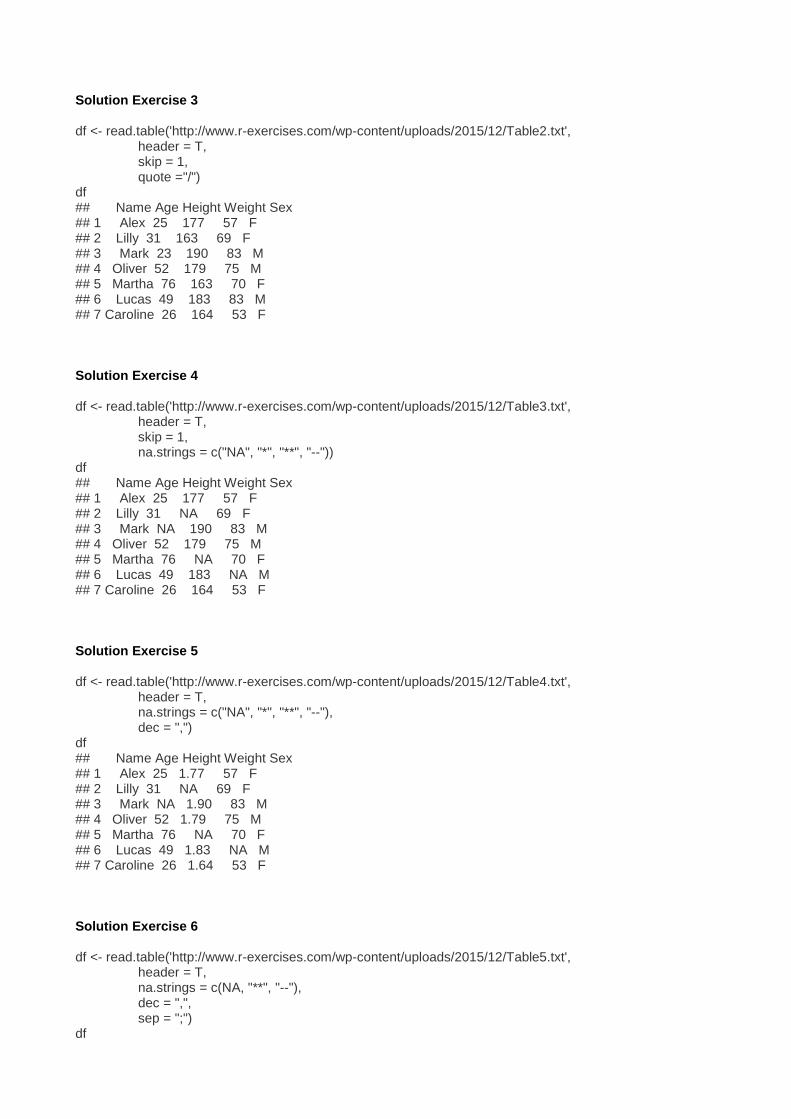
Solution Exercise 3 df <- read.table('http://www.r-exercises.com/wp-content/uploads/2015/12/Table2.txt', header = T, skip = 1, quote ="/") df ## Name Age Height Weight Sex ## 1 Alex 25 177 57 F ## 2 Lilly 31 163 69 F ## 3 Mark 23 190 83 M ## 4 Oliver 52 179 75 M ## 5 Martha 76 163 70 F ## 6 Lucas 49 183 83 M ## 7 Caroline 26 164 53 F Solution Exercise 4 df <- read.table('http://www.r-exercises.com/wp-content/uploads/2015/12/Table3.txt', header = T, skip = 1, na.strings = c("NA", "*", "**", "--")) df ## Name Age Height Weight Sex ## 1 Alex 25 177 57 F ## 2 Lilly 31 NA 69 F ## 3 Mark NA 190 83 M ## 4 Oliver 52 179 75 M ## 5 Martha 76 NA 70 F ## 6 Lucas 49 183 NA M ## 7 Caroline 26 164 53 F Solution Exercise 5 df <- read.table('http://www.r-exercises.com/wp-content/uploads/2015/12/Table4.txt', header = T, na.strings = c("NA", "*", "**", "--"), dec = ",") df ## Name Age Height Weight Sex ## 1 Alex 25 1.77 57 F ## 2 Lilly 31 NA 69 F ## 3 Mark NA 1.90 83 M ## 4 Oliver 52 1.79 75 M ## 5 Martha 76 NA 70 F ## 6 Lucas 49 1.83 NA M ## 7 Caroline 26 1.64 53 F Solution Exercise 6 df <- read.table('http://www.r-exercises.com/wp-content/uploads/2015/12/Table5.txt', header = T, na.strings = c(NA, "**", "--"), dec = ",", sep = ";") df

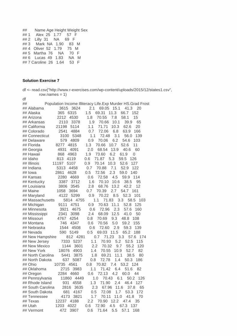
## Name Age Height Weight Sex ## 1 Alex 25 1.77 57 F ## 2 Lilly 31 NA 69 F ## 3 Mark NA 1.90 83 M ## 4 Oliver 52 1.79 75 M ## 5 Martha 76 NA 70 F ## 6 Lucas 49 1.83 NA M ## 7 Caroline 26 1.64 53 F Solution Exercise 7 df <- read.csv("http://www.r-exercises.com/wp-content/uploads/2015/12/states1.csv", row.names = 1) df ## Population Income Illiteracy Life.Exp Murder HS.Grad Frost ## Alabama 3615 3624 2.1 69.05 15.1 41.3 20 ## Alaska 365 6315 1.5 69.31 11.3 66.7 152 ## Arizona 2212 4530 1.8 70.55 7.8 58.1 15 ## Arkansas 2110 3378 1.9 70.66 10.1 39.9 65 ## California 21198 5114 1.1 71.71 10.3 62.6 20 ## Colorado 2541 4884 0.7 72.06 6.8 63.9 166 ## Connecticut 3100 5348 1.1 72.48 3.1 56.0 139 ## Delaware 579 4809 0.9 70.06 6.2 54.6 103 ## Florida 8277 4815 1.3 70.66 10.7 52.6 11 ## Georgia 4931 4091 2.0 68.54 13.9 40.6 60 ## Hawaii 868 4963 1.9 73.60 6.2 61.9 0 ## Idaho 813 4119 0.6 71.87 5.3 59.5 126 ## Illinois 11197 5107 0.9 70.14 10.3 52.6 127 ## Indiana 5313 4458 0.7 70.88 7.1 52.9 122 ## Iowa 2861 4628 0.5 72.56 2.3 59.0 140 ## Kansas 2280 4669 0.6 72.58 4.5 59.9 114 ## Kentucky 3387 3712 1.6 70.10 10.6 38.5 95 ## Louisiana 3806 3545 2.8 68.76 13.2 42.2 12 ## Maine 1058 3694 0.7 70.39 2.7 54.7 161 ## Maryland 4122 5299 0.9 70.22 8.5 52.3 101 ## Massachusetts 5814 4755 1.1 71.83 3.3 58.5 103 ## Michigan 9111 4751 0.9 70.63 11.1 52.8 125 ## Minnesota 3921 4675 0.6 72.96 2.3 57.6 160 ## Mississippi 2341 3098 2.4 68.09 12.5 41.0 50 ## Missouri 4767 4254 0.8 70.69 9.3 48.8 108 ## Montana 746 4347 0.6 70.56 5.0 59.2 155 ## Nebraska 1544 4508 0.6 72.60 2.9 59.3 139 ## Nevada 590 5149 0.5 69.03 11.5 65.2 188 ## New Hampshire 812 4281 0.7 71.23 3.3 57.6 174 ## New Jersey 7333 5237 1.1 70.93 5.2 52.5 115 ## New Mexico 1144 3601 2.2 70.32 9.7 55.2 120 ## New York 18076 4903 1.4 70.55 10.9 52.7 82 ## North Carolina 5441 3875 1.8 69.21 11.1 38.5 80 ## North Dakota 637 5087 0.8 72.78 1.4 50.3 186 ## Ohio 10735 4561 0.8 70.82 7.4 53.2 124 ## Oklahoma 2715 3983 1.1 71.42 6.4 51.6 82 ## Oregon 2284 4660 0.6 72.13 4.2 60.0 44 ## Pennsylvania 11860 4449 1.0 70.43 6.1 50.2 126 ## Rhode Island 931 4558 1.3 71.90 2.4 46.4 127 ## South Carolina 2816 3635 2.3 67.96 11.6 37.8 65 ## South Dakota 681 4167 0.5 72.08 1.7 53.3 172 ## Tennessee 4173 3821 1.7 70.11 11.0 41.8 70 ## Texas 12237 4188 2.2 70.90 12.2 47.4 35 ## Utah 1203 4022 0.6 72.90 4.5 67.3 137 ## Vermont 472 3907 0.6 71.64 5.5 57.1 168

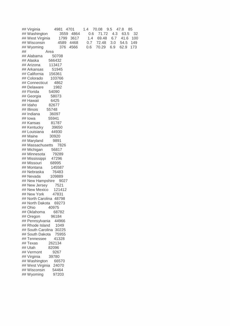
## Virginia 4981 4701 1.4 70.08 9.5 47.8 85 ## Washington 3559 4864 0.6 71.72 4.3 63.5 32 ## West Virginia 1799 3617 1.4 69.48 6.7 41.6 100 ## Wisconsin 4589 4468 0.7 72.48 3.0 54.5 149 ## Wyoming 376 4566 0.6 70.29 6.9 62.9 173 ## Area ## Alabama 50708 ## Alaska 566432 ## Arizona 113417 ## Arkansas 51945 ## California 156361 ## Colorado 103766 ## Connecticut 4862 ## Delaware 1982 ## Florida 54090 ## Georgia 58073 ## Hawaii 6425 ## Idaho 82677 ## Illinois 55748 ## Indiana 36097 ## Iowa 55941 ## Kansas 81787 ## Kentucky 39650 ## Louisiana 44930 ## Maine 30920 ## Maryland 9891 ## Massachusetts 7826 ## Michigan 56817 ## Minnesota 79289 ## Mississippi 47296 ## Missouri 68995 ## Montana 145587 ## Nebraska 76483 ## Nevada 109889 ## New Hampshire 9027 ## New Jersey 7521 ## New Mexico 121412 ## New York 47831 ## North Carolina 48798 ## North Dakota 69273 ## Ohio 40975 ## Oklahoma 68782 ## Oregon 96184 ## Pennsylvania 44966 ## Rhode Island 1049 ## South Carolina 30225 ## South Dakota 75955 ## Tennessee 41328 ## Texas 262134 ## Utah 82096 ## Vermont 9267 ## Virginia 39780 ## Washington 66570 ## West Virginia 24070 ## Wisconsin 54464 ## Wyoming 97203

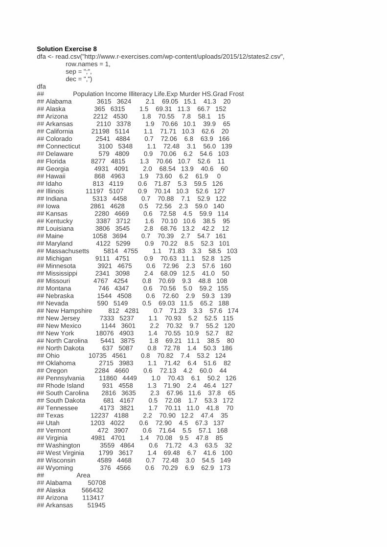
Solution Exercise 8 dfa <- read.csv("http://www.r-exercises.com/wp-content/uploads/2015/12/states2.csv", row.names = 1, sep = ";", dec = ",") dfa ## Population Income Illiteracy Life.Exp Murder HS.Grad Frost ## Alabama 3615 3624 2.1 69.05 15.1 41.3 20 ## Alaska 365 6315 1.5 69.31 11.3 66.7 152 ## Arizona 2212 4530 1.8 70.55 7.8 58.1 15 ## Arkansas 2110 3378 1.9 70.66 10.1 39.9 65 ## California 21198 5114 1.1 71.71 10.3 62.6 20 ## Colorado 2541 4884 0.7 72.06 6.8 63.9 166 ## Connecticut 3100 5348 1.1 72.48 3.1 56.0 139 ## Delaware 579 4809 0.9 70.06 6.2 54.6 103 ## Florida 8277 4815 1.3 70.66 10.7 52.6 11 ## Georgia 4931 4091 2.0 68.54 13.9 40.6 60 ## Hawaii 868 4963 1.9 73.60 6.2 61.9 0 ## Idaho 813 4119 0.6 71.87 5.3 59.5 126 ## Illinois 11197 5107 0.9 70.14 10.3 52.6 127 ## Indiana 5313 4458 0.7 70.88 7.1 52.9 122 ## Iowa 2861 4628 0.5 72.56 2.3 59.0 140 ## Kansas 2280 4669 0.6 72.58 4.5 59.9 114 ## Kentucky 3387 3712 1.6 70.10 10.6 38.5 95 ## Louisiana 3806 3545 2.8 68.76 13.2 42.2 12 ## Maine 1058 3694 0.7 70.39 2.7 54.7 161 ## Maryland 4122 5299 0.9 70.22 8.5 52.3 101 ## Massachusetts 5814 4755 1.1 71.83 3.3 58.5 103 ## Michigan 9111 4751 0.9 70.63 11.1 52.8 125 ## Minnesota 3921 4675 0.6 72.96 2.3 57.6 160 ## Mississippi 2341 3098 2.4 68.09 12.5 41.0 50 ## Missouri 4767 4254 0.8 70.69 9.3 48.8 108 ## Montana 746 4347 0.6 70.56 5.0 59.2 155 ## Nebraska 1544 4508 0.6 72.60 2.9 59.3 139 ## Nevada 590 5149 0.5 69.03 11.5 65.2 188 ## New Hampshire 812 4281 0.7 71.23 3.3 57.6 174 ## New Jersey 7333 5237 1.1 70.93 5.2 52.5 115 ## New Mexico 1144 3601 2.2 70.32 9.7 55.2 120 ## New York 18076 4903 1.4 70.55 10.9 52.7 82 ## North Carolina 5441 3875 1.8 69.21 11.1 38.5 80 ## North Dakota 637 5087 0.8 72.78 1.4 50.3 186 ## Ohio 10735 4561 0.8 70.82 7.4 53.2 124 ## Oklahoma 2715 3983 1.1 71.42 6.4 51.6 82 ## Oregon 2284 4660 0.6 72.13 4.2 60.0 44 ## Pennsylvania 11860 4449 1.0 70.43 6.1 50.2 126 ## Rhode Island 931 4558 1.3 71.90 2.4 46.4 127 ## South Carolina 2816 3635 2.3 67.96 11.6 37.8 65 ## South Dakota 681 4167 0.5 72.08 1.7 53.3 172 ## Tennessee 4173 3821 1.7 70.11 11.0 41.8 70 ## Texas 12237 4188 2.2 70.90 12.2 47.4 35 ## Utah 1203 4022 0.6 72.90 4.5 67.3 137 ## Vermont 472 3907 0.6 71.64 5.5 57.1 168 ## Virginia 4981 4701 1.4 70.08 9.5 47.8 85 ## Washington 3559 4864 0.6 71.72 4.3 63.5 32 ## West Virginia 1799 3617 1.4 69.48 6.7 41.6 100 ## Wisconsin 4589 4468 0.7 72.48 3.0 54.5 149 ## Wyoming 376 4566 0.6 70.29 6.9 62.9 173 ## Area ## Alabama 50708 ## Alaska 566432 ## Arizona 113417 ## Arkansas 51945

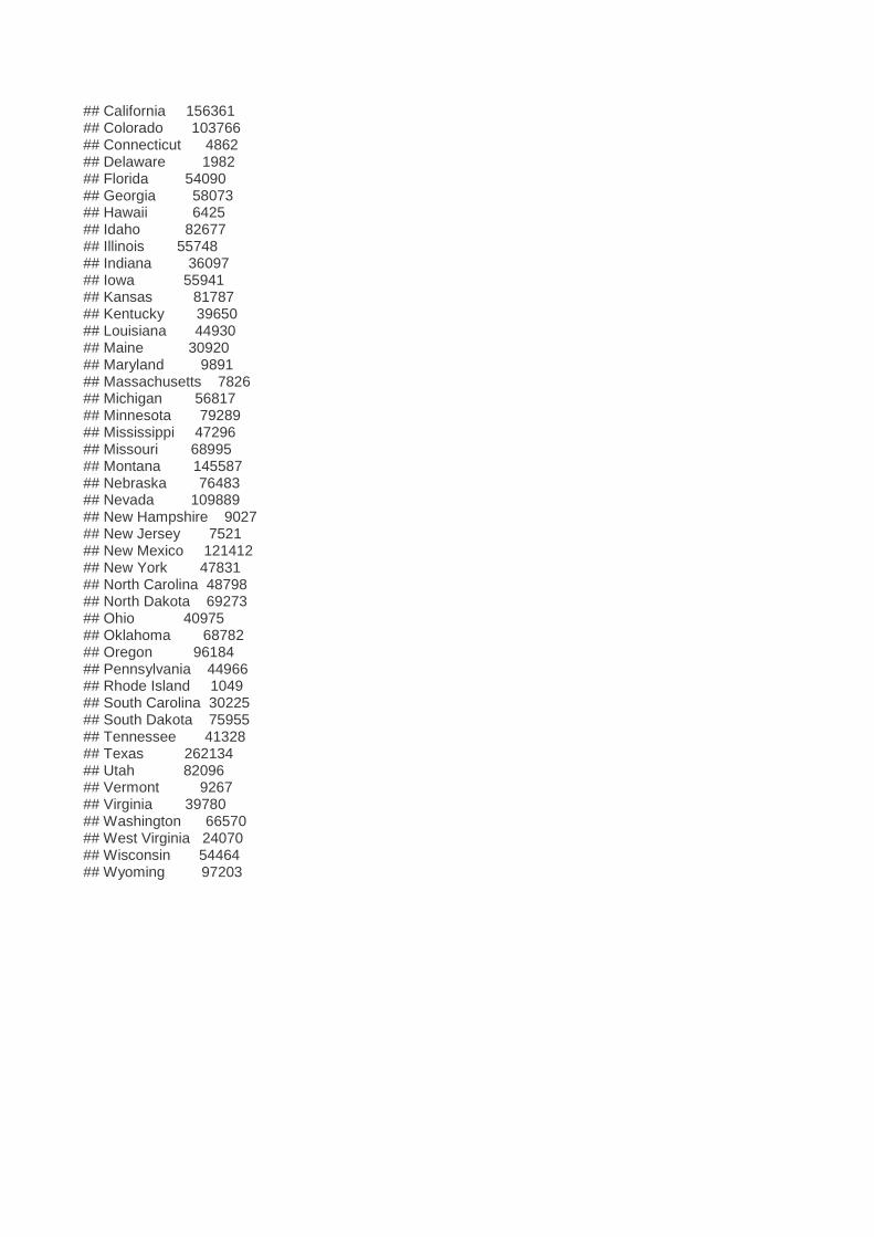
## California 156361 ## Colorado 103766 ## Connecticut 4862 ## Delaware 1982 ## Florida 54090 ## Georgia 58073 ## Hawaii 6425 ## Idaho 82677 ## Illinois 55748 ## Indiana 36097 ## Iowa 55941 ## Kansas 81787 ## Kentucky 39650 ## Louisiana 44930 ## Maine 30920 ## Maryland 9891 ## Massachusetts 7826 ## Michigan 56817 ## Minnesota 79289 ## Mississippi 47296 ## Missouri 68995 ## Montana 145587 ## Nebraska 76483 ## Nevada 109889 ## New Hampshire 9027 ## New Jersey 7521 ## New Mexico 121412 ## New York 47831 ## North Carolina 48798 ## North Dakota 69273 ## Ohio 40975 ## Oklahoma 68782 ## Oregon 96184 ## Pennsylvania 44966 ## Rhode Island 1049 ## South Carolina 30225 ## South Dakota 75955 ## Tennessee 41328 ## Texas 262134 ## Utah 82096 ## Vermont 9267 ## Virginia 39780 ## Washington 66570 ## West Virginia 24070 ## Wisconsin 54464 ## Wyoming 97203

SOURCE: https://www.r-exercises.com/2016/03/11/start-plotting-data-3/

PLOTTING DATA

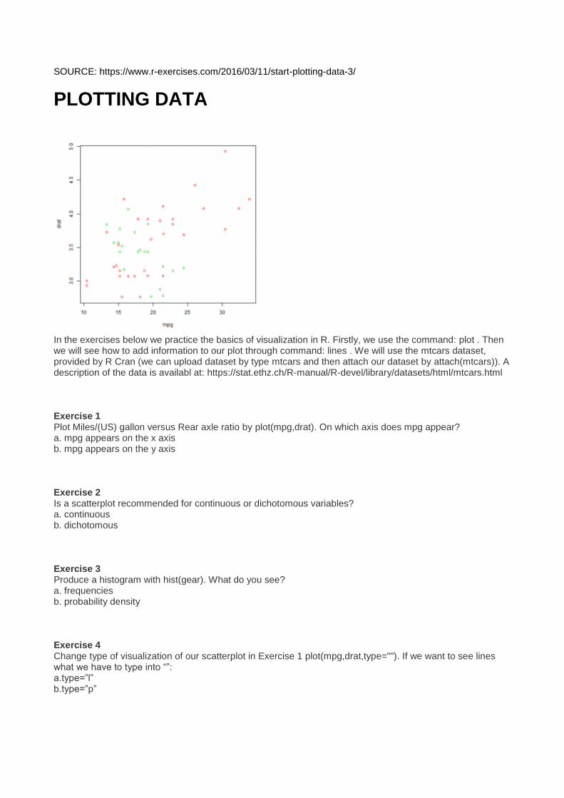
In the exercises below we practice the basics of visualization in R. Firstly, we use the command: plot . Then we will see how to add information to our plot through command: lines . We will use the mtcars dataset, provided by R Cran (we can upload dataset by type mtcars and then attach our dataset by attach(mtcars)). A description of the data is availabl at: https://stat.ethz.ch/R-manual/R-devel/library/datasets/html/mtcars.html Exercise 1 Plot Miles/(US) gallon versus Rear axle ratio by plot(mpg,drat). On which axis does mpg appear? a. mpg appears on the x axis b. mpg appears on the y axis Exercise 2 Is a scatterplot recommended for continuous or dichotomous variables? a. continuous b. dichotomous Exercise 3 Produce a histogram with hist(gear). What do you see? a. frequencies b. probability density Exercise 4 Change type of visualization of our scatterplot in Exercise 1 plot(mpg,drat,type=""). If we want to see lines what we have to type into “”: a.type=”l” b.type=”p”

Exercise 5 Now we want to see both point and lines in our plot. What we have to type into plot(mpg,drat,type=""): a.type=c(“p”,”l”) b.type=”b” Exercise 6 Add another variable to our plot, for example Weight. What command do we have to use: a.plot(mpg, drat); plot(mpg, wt) b.plot(mpg, drat); points(mpg, wt) Exercise 7 Now we have added a new variable to our plot. Suppose we want to use two different colours to separate the points. Type plot(mpg, drat, col=2) : What colour have we selected: a. red b. green Exercise 8 Now we want to differentiate the two different variables in the scatterplot: a. Let’s change the colours of the second plot b. Change use two different types of plot (e.g. points,lines) Exercise 9 Now we want to highlight a variable in the final plot. Type: plot(mpg, drat, lwd=2) ; points(mpg, wt, lwd=1). Which plot is highlighted: a. plot1 (mpg,drat) b. plot2 (mpg,wt) Exercise 10 Finally choose four different continuous variables from mtcars set and produce: a.Plot with lines and points for different variables with different colours (hint: change y axis parameters by adding command ylim=c(0,30) to plot [e.g. plot(a,b,type="p",ylim=c(0,30)). b.Choose one variable from each and highlighted it set red colour and a broad line.

SOURCE: https://www.r-exercises.com/2016/03/11/start-plotting-data-solutions/

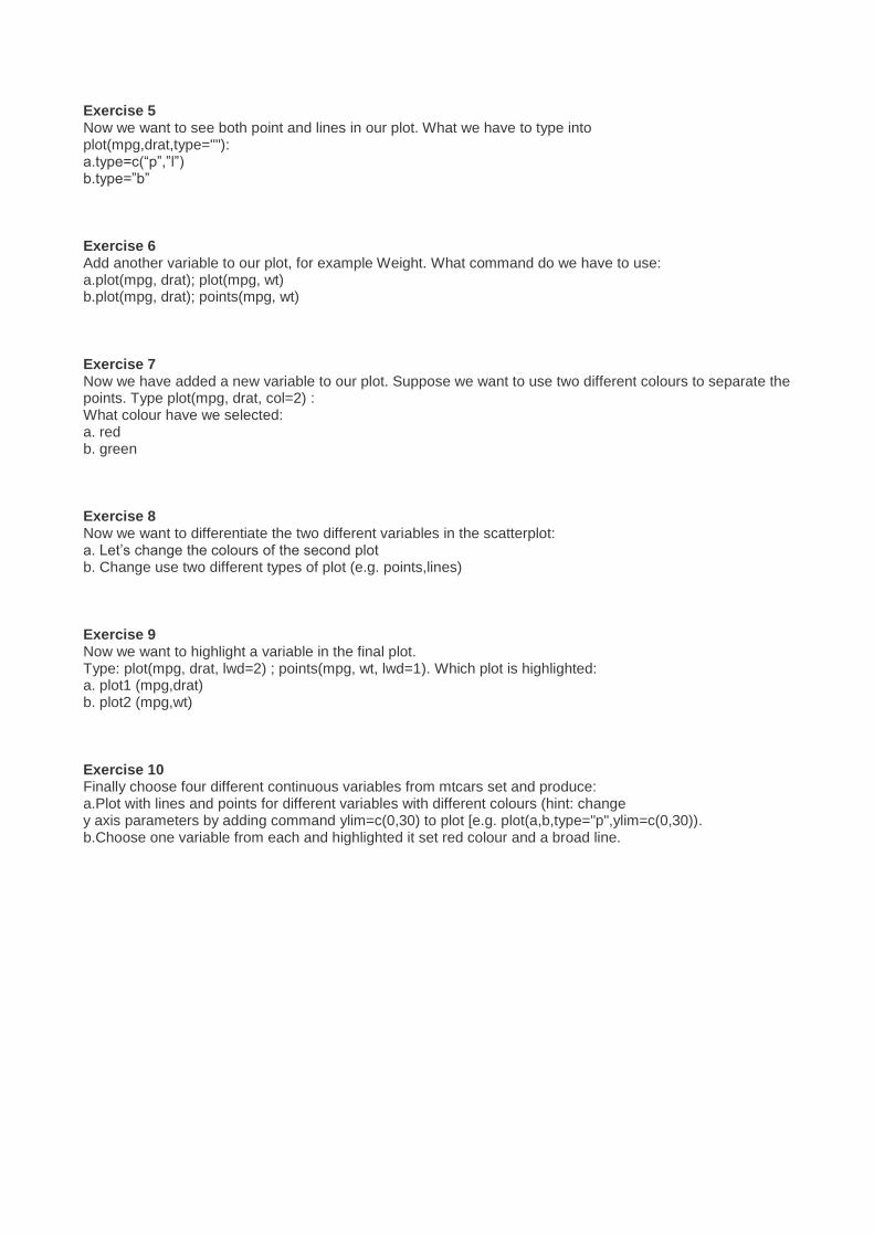
PLOTTING DATA: SOLUTIONS Solution Exercise 1 attach(mtcars) plot(mpg,drat)

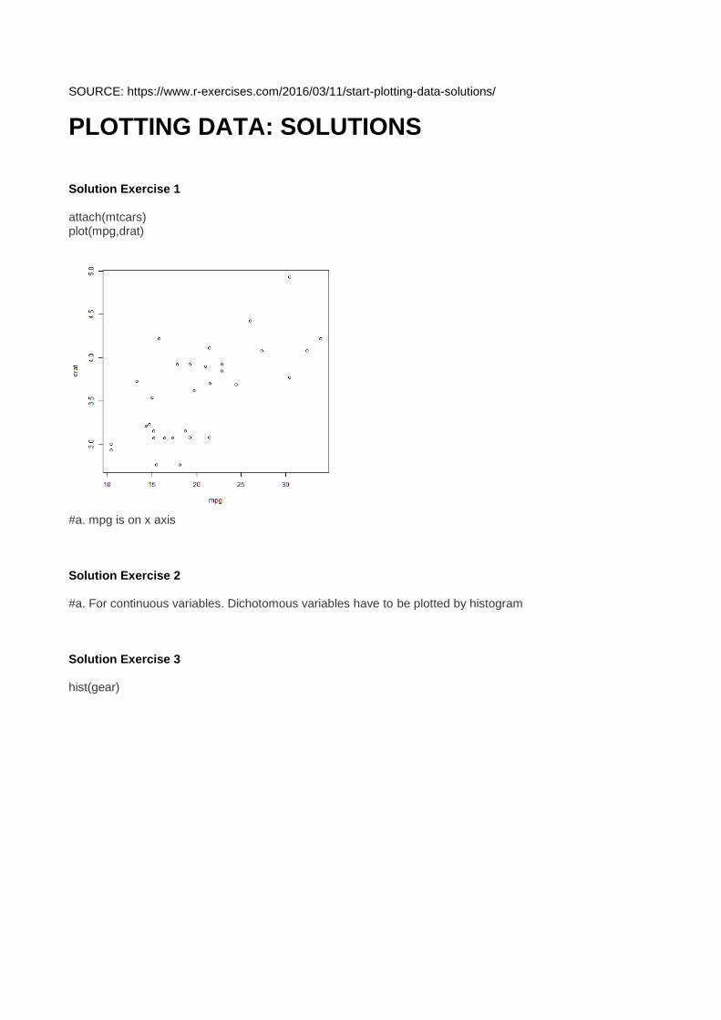
#a. mpg is on x axis Solution Exercise 2 #a. For continuous variables. Dichotomous variables have to be plotted by histogram Solution Exercise 3 hist(gear)

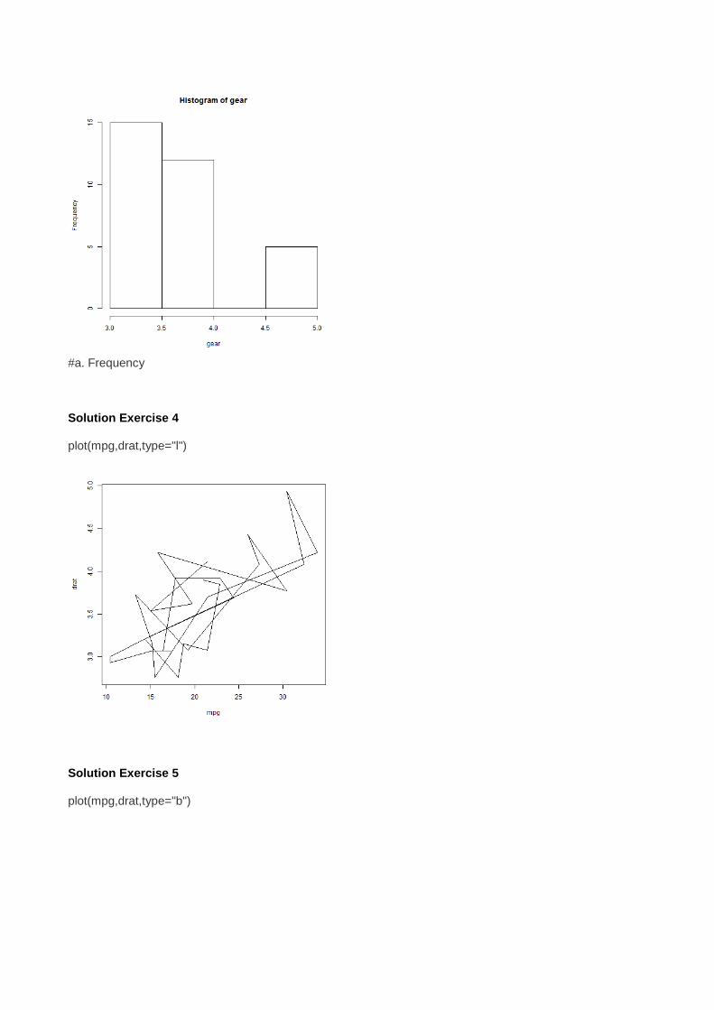
#a. Frequency Solution Exercise 4 plot(mpg,drat,type="l")

Solution Exercise 5 plot(mpg,drat,type="b")

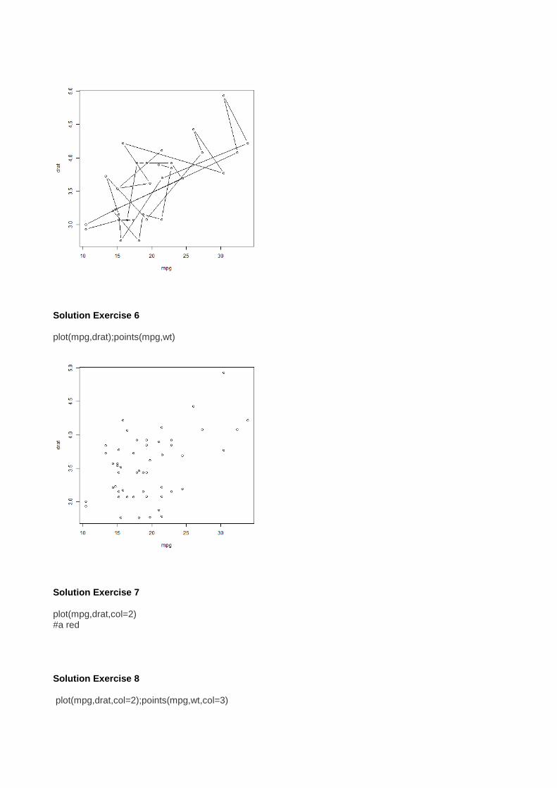
Solution Exercise 6 plot(mpg,drat);points(mpg,wt)

Solution Exercise 7 plot(mpg,drat,col=2) #a red Solution Exercise 8 plot(mpg,drat,col=2);points(mpg,wt,col=3)

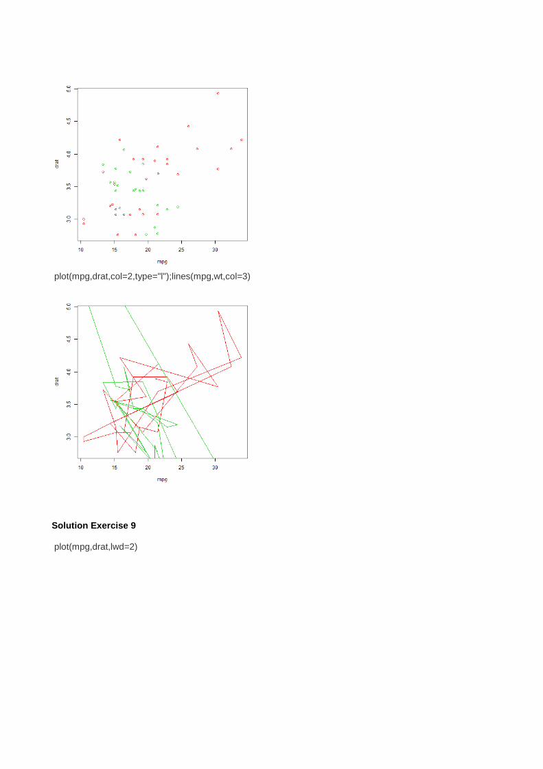
plot(mpg,drat,col=2,type="l");lines(mpg,wt,col=3)

Solution Exercise 9 plot(mpg,drat,lwd=2)

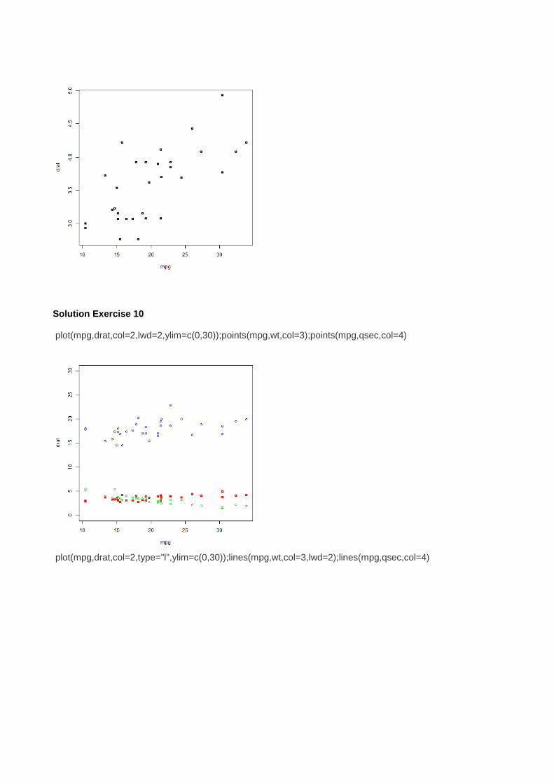
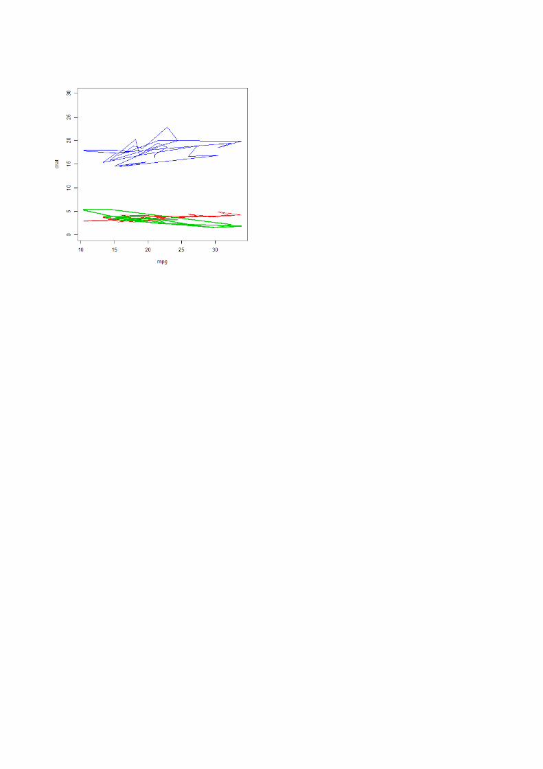
Solution Exercise 10 plot(mpg,drat,col=2,lwd=2,ylim=c(0,30));points(mpg,wt,col=3);points(mpg,qsec,col=4)

plot(mpg,drat,col=2,type="l",ylim=c(0,30));lines(mpg,wt,col=3,lwd=2);lines(mpg,qsec,col=4)