Transfer Prices and Import and Export Price Indexes: Theory and Practice 1

(June 4, 2004 version)

W. Erwin Diewert Department of Economics

University of British Columbia Vancouver, Canada, V6T 1Z1 Email:diewert@econ.ubc.ca

William F. Alterman

Division of International Prices Bureau of Labor Statistics

2 Massachusetts Avenue, N. E. Washington DC 20212

Email: alterman_w@bls.gov

Lorraine Eden Department of Management

Texas A&M University TAMU 4221

College Station, Texas 77843-4221 Email: leden@tamu.edu

1 The authors thank Ted To for helpful comments. All views expressed in this paper are those of the authors and do not necessarily reflect the views or policies of the U.S. Bureau of Labor Statistics.

2

1. Introduction The main purpose of this paper is to suggest a theoretical foundation for determining what is the appropriate price a statistical agency (like the Bureau of Labor Statistics) should seek from domestic establishments that engage in international trade with an affiliated establishment abroad. Such a price is called a transfer price. Should such a price be the same price that the related party reports to the relevant domestic trade authority such as the U. S. Customs Service for the U. S.? Or should it be the price that is reported to the domestic tax authority such as the Internal Revenue Service for the U. S. case? Or should it be a cost based price? Or should it be a market based price for similar trades with unaffiliated establishments? Finally, suppose that the conceptually perfect transfer price cannot be collected for practical reasons. In this situation, what are the practical alternatives for the price collector and can they be ordered in terms of their desirability? These are the questions that we will attempt to answer in this paper. What makes a transfer price different from a price for an international trade transaction between two unrelated firms? When there is a international transaction between say two divisions of a multinational enterprise (MNE), then the value of the transaction to the exporting division will be equal to the value of the transaction for the importing division and when the MNE works out its profits worldwide for the quarter where the transaction took place, the export value will equal the import value and hence will cancel out, leaving the MNE’s overall profits unchanged, no matter what price it chooses to value the transaction.2 Hence, at first glance, it appears that the firm could choose the transfer price for the transaction to be practically anything.3 However, in a world where there are taxes on international transactions and where the rates of business income taxation differ across countries, then as we shall see below, the situation is actually worse: in this situation, the multinational will have definite financial incentives to choose strategically the transfer price to minimize the amount of taxation paid to both jurisdictions. It is this element of strategic choice that casts doubt on the usefulness of simply collecting transfer prices just as if they were ordinary prices between unrelated parties. However, if we choose to question reported transfer prices, what type of price should replace them? This question will be addressed in section 13 of this paper. Before the transfer price problem is directly addressed, some background information detailing the importance and complexity of pricing intra-firm trade will be found in section 2. It will be followed by a brief overview in section 3 of some of the purposes that indexes of export and import prices might be used. In section 4, we look at some alternative pricing concepts that

2 This assertion requires the proviso that there are no trade taxes on the transaction and that business income tax rates are equal in both countries. 3 Thus this situation is very different than that where the trade takes place between unaffiliated firms. In the latter case, the price for the transaction is very meaningful: an increase in the negotiated price will increase the profits of one firm and decrease the profits of the other firm.

2

could be used to describe import and export prices that could be used in a national index of import or export prices. In section 5, we define in a preliminary fashion the four main types of transfer price that have been considered in the theoretical literature on transfer prices. In this section, the transfer price problem is studied in the context of two affiliated establishments in two countries trading a single commodity. In section 6, we consider the simplest case where there are no trade taxes, business income taxes do not exist (or are the same in the two jurisdictions) and there is an external market price for the traded commodity. In section 7, we consider the case where there are no trade or business income tax distortions but an external market for the internationally traded commodity does not exist. In sections 8-10, the analysis is extended to the case where the rates of business income taxation differ in the two countries (section 8), to the case where the rate of business taxation are the same but there are trade taxes (section 9) and finally to the situation where there are both trade taxes and differing rates of business income taxation (section 10). Although this framework is rather simple, most of the complexities of transfer pricing can be illustrated using it. Sections 11 and 12 look at “practical” approximations to the theoretical transfer price in the context of a single commodity traded internationally between related establishments. Section 13 looks at the main question that we are attempting to answer, namely, what are the practical alternatives for collecting transfer prices and can they be ordered in terms of their desirability? This section concludes with some additional discussion of what can be done at the central office in order to obtain improved transfer prices. The theory presented in sections 6-12 assumes that the importing and exporting establishments behave competitively; i.e., they take the prices of nontraded commodities as being fixed parameters beyond their control. An Appendix considers how the theoretical results are changed when this assumption is relaxed. 2. Background The need to calculate accurately prices of goods in intra-firm trade is not just an abstract one. In calendar 2000, the latest year that the data are available, the Bureau of Economic Analysis reported that $241 billion (or 31 percent) of export goods and $452 billion (or 37 percent) of imports were between related parties. During the past 20 years these percentages have tended to fluctuate somewhat. The value for exports has ranged between 31 and 40 percent, while the comparable range for imports is between 37 and 44 percent. Regardless of the actual percentage, intra-firm shipments continue to represent a substantial portion of U.S. trade.4 It should be noted that the characteristics of intra-firm trade could be different from trade between unrelated parties. For example, in 2001, only 13 percent of exports to both China and Korea were intra-firm, while 41 percent of sales to Mexico were between related parties. On the

4 The percentage figures constructed using the BLS price data (which uses a separate survey compared to the data produced by the U.S. Customs Service or BEA) are similar.

3

import side, fully 74 percent of U.S. imports from Japan were related party trade, while the comparable figure for China was just 18 percent. Similar differences crop up when looking at the data by industry, with especially high proportions of intra-firm trade in transportation equipment, computers and chemicals.5 Even within intra-firm trade their can be significant differences. For U.S. multinationals, 65 percent of their exports in 1999 consisted of intermediate products exported to overseas affiliates for further processing or assembly. In contrast, for foreign multinationals 76 percent of their shipments to the U.S. in 1998 were finished goods ready for final sale.6 Given these types of variations, simply excluding intra-firm trade when constructing export and import price indexes would not be appropriate. Because of the significant international taxation aspects of world trade, the pricing of goods in intra-firm trade has become a major issue, both politically as well as administratively. It has been contended that companies do indeed price these goods in order to maximize corporate profits. Using BLS price data, a recent paper found evidence that “there is a strong and statistically significant relationship between countries’ tax rates and the prices of intra-firm imports and exports exchange with those countries.”7 A Federally funded study released in October 2002 by Professors Simon J. Pak and John S. Zdanowicz, estimated that corporations saved $53.1 billion in 2001 by over or under invoicing goods in intra-firm trade. The evidence on transfer price manipulation is, however, mixed (Eden, 1998; 2001b). Ernst & Young (2003, p. 17), for example, reports that over 80% of MNE parent respondents “use a single set of transfer prices for management and tax purposes”. Twenty-five percent of respondents said that “business strategy drives all transfer pricing decisions”, with almost 40% of respondents reporting that “management and operational objectives are more important than fiscal considerations”. To the extent that the Ernst & Young (2003) report is an accurate reflection of MNE transfer pricing practices, concerns over strategic transfer pricing should be somewhat tempered. Nonetheless, politicians and academics alike are taking a closer look at these and other possible practices used by multinationals to minimize corporate taxes.8 From an administrative standpoint, the pricing of U.S. goods in international trade must serve two masters: The Internal Revenue Service (IRS) and the U.S. Customs Service.9 While

5 These data are from the Bureau of the Census (2002). Although the Census data is not considered as accurate as data from BEA, the aggregate numbers are fairly consistent. 6 The best article on the value of intra-firm trade was published in 1997 by the Bureau of Economic Analysis; see Zeile (1997). In addition, more recent data is available directly from BEA. 7 See Clausing (2001). 8 The Pak-Zdanowicz study was funded at the behest of Senator Byron Dorgan (Democrat, North Dakota) who has been critical of both multinationals as well as the Treasury Department. Pak and Zdanowicz (2002) is an executive summary of this study. For Senator Dorgan’s comments, see Dorgan (2002). For an example of ongoing attempts by Congress to address other multinational practices for reducing taxes (such as incorporating in a low tax jurisdiction), see Freedman (2002). 9 Note that, in general, the valuation of transactions between domestic buyers and sellers are not subject to the same government scrutiny. This is for two reasons: first, most of these transactions are between unrelated parties; and second, the tax implications of these transactions

4

Federal—and most foreign--regulations call for the use of an arm’s length standard in valuing intra-firm trade, these two agencies historically have worked independently in deriving values for intra-firm trade, in part because they have differing objectives.10 Tariff officials, who are attempting to maximize duty assessments, will tend to want to raise the value of imported goods, while the IRS will have a tendency to want to lower the value of imports in order to maximize the amount of domestic profits.11 Furthermore, while Customs values tend to be finalized comparatively quickly, final valuations associate with IRS audits and subsequent court procedures can drag on for years.12 The laws, procedures and documentation covering transfer prices are complicated and substantial. Both agencies devote significant resources to pricing intra-firm trade. This brief summary of the US situation, of course, does not even address the transfer price regulations associated with other countries.13 Because of this complexity, corporations can end up devoting substantial resources to valuing intra-firm trade.14 In a recent survey, fifty-nine percent of multinationals indicated that they had undergone an audit of their transfer pricing practices in 2001.15 Increasingly multinational traders avail themselves of any number of accounting firms that specialize in assisting corporations in navigating the multitude of both domestic and foreign regulations associated with pricing intra-firm trade. In the early 1990s, in order to minimize the disagreements between importers and the IRS, the IRS introduced Advanced Pricing Agreements (APA) whereby a company could voluntary meet with the IRS and negotiate a transfer pricing method that would stand for a fixed length of time, usually five years. While designed to streamline the process, it nonetheless, has added more complexity to the pricing process.16 Since individual APAs are considered confidential, it is not clear how they are constructed and how often they are used.

are minimal. An official of the Bureau of the Census, which is responsible for collecting data on domestic shipments from manufacturers, did confirm that companies oftentimes had problems valuing shipments between plants that were within the same firm, particularly when the item was an intermediate good which would undergo further processing prior to being sold. Unfortunately, the Bureau of the Census does not publish separate totals for related and unrelated value of domestic shipments. (as per conversation with Judy M. Dodds, May 25th, 2004). 10 Under an Arm’s Length Standard, the transfer price should equal the price that would be settled on if the two trading firms were unrelated. 11 See Eden (1998; 395-96) for further details. 12 See Eden (1998; 684) for mention of 4 cases that each dragged on for over a decade. 13 It should also be noted that export data do not receive nearly the same scrutiny as import data from the U.S. Customs Service. In fact, since 1990 the U.S. has used data supplied by Statistics Canada to estimate U.S. exports to Canada. In 1986 undocumented U.S. exports to Canada were equivalent to 22.4 percent of the published value; see Mozes and Oberg (2002). 14 The IRS, at the behest of Senate Committee on Appropriations, even contracted for a study assessing the cost to business of filing the paperwork associated with intra-firm trade; see Schulman, Ronca and Bucuvalas, Inc. (2001). 15 The survey indicated that the rate for was even higher when looking at just U.S. trade; see Ernst & Young (2001). 16 APAs can still be very detailed and a number of companies such as Ernst & Young, and Deloitte & Touche advertise their services extensively. For example, see Deloitte & Touche (2002), which is essentially an advertisement, detailing their services.

5

The limited evidence available, however, indicates that APAs cover a significant portion of U.S. trade in goods, services and intangibles.17 Furthermore, there is a concern that companies are able to use APAs to minimize taxes. Consequently, the U.S. Senate Committee on Finance has requested the IRS investigate and report back to Congress on the effectiveness of the APA program.18 Some of the companies which have publicly announced that they make use of APAs include Ford Motor Company, Apple Computer Incorporated, Sony Corporation of America and Intel Corporation. All of this serves to emphasize both the importance of transfer pricing as well as the difficulty in estimating these prices. Since transfer prices are used in export and import price indexes, the next section will review some of the purposes and uses of these indexes. 3. Import and Export Price Indexes: Purposes and Uses There are many purposes for national import and export price indexes. In this section, we list seven of the major uses and purposes. (a) Calculation of a Country’s Terms of Trade A country’s terms of trade is defined as an index of export prices divided by an index of import prices. To illustrate this concept, assume for simplicity that there is only one exported commodity that has price px

t in period t and one imported commodity into the country that has price pm

t in period t. Then the terms of trade for the country, comparing the prices in period 0 with those of period t, is defined as follows: (1) TT(0,t) ≡ [px

t/px0]/[pm

t/pm0] .

Thus the terms of trade is the rate of increase in export prices going from a base period to the current period divided by the corresponding rate of increase in import prices. If the terms of trade is greater than 1, we say that there has been an improvement in the country’s terms of trade while if TT(0,t) is less than 1, we say that there has been a deterioration in the terms of trade. An improvement in the terms of trade means that a country can now purchase additional units of the imported commodity in exchange for a single unit of the export commodity as compared to the situation in the base period; i.e., foreigners offer are now willing to exchange more imports in exchange for a constant amount of exports compared to the base period. Hence, the home

17 During the first 10 years of its existence (1991-2001) 349 APA agreements were executed; see Internal Revenue Service (2002; 8). In 2001 alone, however, 77 applications for an APA were filed, indicating that this practice is becoming more prevalent over time. A report by the General Accounting Office stated that the 10 percent of the major multinationals had an approved APA, but that this 10 percent accounted for 42 percent of the dollar value of the intercompany transactions included in their analysis (2002). For the most recent information see Ernst & Young (2003) for a survey of APA practices, perceptions and trends in 22 countries. 18 “Grassley, Baucus Launch Review of Whether Certain Multinationals Pay Fair Share of Taxes,” Press Release, December 22, 2003.

6

country is now better off.19 A country’s terms of trade index is sometimes viewed as an index of the country’s competitive success in foreign markets. Thus if a country is able to sell its products at higher prices in foreign markets so that its terms of trade increases, then this could be viewed as an improvement in the country’s competitiveness.20 (b) Measurement of National Real Output and Productivity The output of a country is defined in nominal terms as the familiar C + I + G + X − M (consumption plus investment plus government expenditures plus exports minus imports) and in order to define real output, each component of national output has to be deflated by a price index. Hence, a major use for the export and import price index is to act as deflators for two major components of national output so that accurate estimates of real GDP can be constructed. The national productivity of a country is defined as either real output divided by labor input (labor productivity) or as real output divided by real input (multifactor or total factor productivity). Thus import and export price indexes are a necessary input into the construction of national productivity indexes. (c) Measures of National Inflation Central banks require broad indexes of price change or general inflation so that they can undertake monetary policy. Two of the most frequently used indexes of general inflation are the Consumer Price Index and the GDP deflator.21 In order to construct the GDP deflator, price indexes for exports and imports are required. (d) Model Building and Forecasting Price indexes for exports and imports are required for a wide variety of macroeconomic models. More generally, disaggregated models of the economy may require price indexes for a wide

19 Thus an improvement in a country’s terms of trade acts in much the same manner as a productivity improvement, which corresponds to a situation where more output can be produced with the same amount of input. 20 On the other hand, if the country exports mainly primary products, then world commodity prices may simply fluctuate exogenously and the country’s terms of trade may not say much about the country’s competitiveness in international markets. 21 It could be argued that the GDP deflator is not the best index of inflation since import prices enter this index with negative weights. Hence if import prices increase, other things remaining constant, the GDP deflator will decrease. This is a rather counterintuitive property for a measure of general price change. Thus a more appropriate indicator of general inflation might be the deflator for C + I + G + X. Note that a price index for exports will still be required for this inflation index. A price index for imports will be required in order to construct an input price index for the economy. The input price index will be required in order to construct an index of multifactor productivity for the economy but it could also serve as a useful measure of general inflation. See Diewert (2002; 12) for further discussion on these points.

7

variety of components of the exports and imports of a country. Business and government economists are often required to provide forecasts for specific classes of exports and imports in real terms (or they may be asked to forecast future trends in the prices of these components) and price indexes for these components of exports and imports are vital building blocks into their models. (e) Indexation of Contracts An exporter may sign a contract to deliver units of a commodity to a foreign purchaser on a long-term basis. Alternatively, a domestic producer may sign a long-term contract with a foreign supplier in order to ensure delivery of a vital input into the producer’s production process. It may be difficult to determine what a “fair” price for the commodity is for periods that are far off and hence these long-term contracts may use a component of the export or import price index in order to index future prices. Similarly, in the regulatory context, a domestic power company that has to import fuel may be able to pass on part of its costs to demanders by using a formula that involves the import price index for fuel. In all of these indexation uses, it is important that the relevant import or export price index be fairly comprehensive and representative of actual transactions for that component. (f) Monitoring Trade Legislation and Trade Agreements Export and import price indexes can be used to track the effects of various trade policies. For example, the U. S. Department of Commerce may impose a punitive tariff on a certain class of imports (e.g., softwood lumber imports from Canada) in retaliation for perceived unfair trade practices. The import price index for the affected commodity can then be monitored in order to determine whether the foreign exporters are absorbing the tariffs or passing them on to U. S. importers. Similarly, if the government decides to subsidize the exports of a domestic industry, then the relevant export price index could be used to determine whether these exports become more competitive in foreign markets. At times, export and import price indexes play a role in negotiating trade agreements in specific commodity areas. (g) Replacement Cost Accounting If a domestic firm uses replacement cost accounting and it has used imports of foreign machines and equipment in its production process, then it could use the import price index for the relevant class of imports as a price index to escalate the initial purchase cost. From the above list of uses for the components of the export and import price indexes, it can be seen that a modern economy cannot do without these indexes. They are a key input into the national system of economic statistics and they have many other private and public uses. 4. Pricing Concepts In this section, we make some observations on the interaction of the uses of the export and

8

import price indexes with alternative definitions for the price of an export or the price of an import.22 We consider the problem of determining the price for an imported commodity. The problem is that there are several plausible price concepts that can be used in order to price an imported commodity. Consider the problem of importing a particular good from a foreign factory. There is a starting price for this good: the selling price for this good at the foreign factory. This is known as the (output) factory gate price. To this initial price, we need to add transportation costs to ship the good to the port of export in the foreign country plus insurance costs for the inland transportation in the foreign country. Call the resulting price the private opportunity cost export price. Once the good is at the port of export, there may be export subsidies, domestic commodity taxes or additional export taxes that must be paid. After adjusting for government tax and subsidy payments, the resulting price is called the water’s edge export price or the free along side export price. From the viewpoint of the importing country, this price is also known as the free on board import price. This price represents the price that the exporting country is charging international purchasers of the commodity at the exit port of the exporting country. This water’s edge export price is the sum of the private opportunity costs of producing the commodity and shipping it to the export port plus government net taxes that the exporting country sees fit to impose on foreign purchasers of the commodity. This is not the end of the story. To the water’s edge export price, we need to add international shipping and insurance charges to get the commodity to the port of entry of the importing country. The resulting price is called the water’s edge import price. Again, this is not the end of the story. We now can add any applicable domestic commodity taxes and import tariffs to the price (less import subsidies if any) in order to obtain the post tariff import price or the import for consumption price. Finally, we can add to this price, transportation costs to ship the good from the port of entry in the home country to the importing establishment plus the associated insurance costs for the inland transportation in the home country. Call the resulting price the (input) factory gate price. The International Price Program of the Bureau of Labor Statistics attempt to collect the water’s edge export price as its pricing concept for exports (which is the domestic output factory gate price plus domestic inland transportation costs plus U. S. tax and subsidy adjustments). For imports, it attempts to use the foreign water’s edge export price (which is the foreign output factory gate price plus foreign inland transportation costs plus foreign tax and subsidy adjustments). Thus, essentially the same pricing concept is used for both exports and imports.23 This treatment of export and import prices seems to be appropriate if our major purpose is to measure a country’s terms of trade; i.e., what do countries offer us for their exports compared to what we offer foreigners for our exports, exports and imports being priced in a symmetric manner. However, for many of the other purposes listed in section 3 for the import and export price indexes, this treatment will only be approximately “correct”. For purposes (b) and (c), if we are using the economic approach to price and quantity indexes, then the appropriate import pricing concept is either the input factory gate price (since this is the price actually paid for the

22 For additional material on this topic, see Eden (2001) and Eden and Rodriguez (2004). 23 In practice, BLS will accept nearly any price basis that the respondent reports is the basis consistently used in transactions for that particular good. The major exception is on imports where the Bureau will not use prices that include a duty value that cannot be removed.

9

use of the imported commodity by the importing establishment) or the post tariff import price (since this is the price paid for the use of the imported commodity by the consolidated U.S. production sector, including the domestic transportation sector). Similarly, the appropriate export pricing concept is the output factory gate price plus government subsidies since this is the actual revenue received by the producing establishment for producing a unit of the commodity. If we consolidated the exporting establishment with the domestic transportation sector, then the appropriate export pricing concept from the viewpoint of the economic approach to index number theory would be the output factory gate price plus government subsidies plus domestic transportation and insurance costs which is equal to the private opportunity cost export price plus export subsidies.24 Unfortunately, an implication of the above paragraph is that, in theory, more than one export and import index will be required in order to meet the needs of all users of international price indexes. The use of water’s edge prices for imports and exports is suitable if the main purpose of the index is to calculate the country’s terms of trade. For all other uses that use an economic modeling approach that assumes that firms maximize profits or minimize costs, the post tariff price for an imported commodity and the private opportunity cost plus subsidies price for an exported commodity would be the most suitable pricing concepts. If in addition, the effects of domestic trade taxes and subsidies on international trade were to be modeled, then it would also be essential to collect information on taxes paid or subsidies received by domestic exporting and importing establishments. However, it must be recognized that collecting this additional information may place a heavy burden on respondents and price collectors. Indeed, in reality, The Bureau is very limited--both from a legal standpoint, as well as a burden standpoint--in how much additional information can be collected. Like nearly all BLS data collection efforts, the IPP is a voluntary Program and currently approximately 20 percent of the establishments in any given sample refuse to cooperate. The most frequently cited reason for this refusal is burden on the respondent. In addition, any attempt to collect additional information on a regular basis would require approval from the Office of Management and Budget. 5. Alternative Transfer Pricing Concepts There are four main theoretical concepts for a transfer price.25 These concepts are:

• the external market or arm’s length transfer price26;

24 We mention these complications because as noted above, in order to deal with transfer prices in the context of index number theory, it is necessary to use the economic approach to index number theory. However, the economic approach to index number theory requires that the prices used be the prices that firms actually get for their sales of products and the prices that they actually pay out for their inputs. For an exposition of the economic approach to export and import price indexes, see Alterman, Diewert and Feenstra (1999). These theories draw heavily on the theory of the output price index; see Fisher and Shell (1972), Samuelson and Swamy (1974; 588-592), Archibald (1977; 60-61) and Diewert (1980; 461) (1983; 1055). 25 Diewert (1985) considers other transfer pricing concepts but for our purposes, they are not important. Some of these alternative concepts will be mentioned in footnotes below.

10

• the efficient transfer price; • the profit maximizing transfer price and • the economic transfer price that is suitable for collection by a statistical agency.

The first concept for a transfer price is feasible if there is a well-defined external market price for the traded commodity where units can be bought or sold at a common price (let us call it ‘w’). Then the transfer price for the commodity is just this price w. This is the arm’s length transfer price. The second concept for a transfer price arises if there is no external market for the commodity that is traded between two production units (or establishments) of a multinational that are located in different countries. The efficient transfer price is generated by solving a joint profit maximization problem involving the two establishments and it is a Lagrange multiplier, or shadow price, which corresponds to the constraint that says the output of the producing establishment must equal the input of the purchasing establishment. If there are no tax distortions27, then this transfer price can also be generated by setting up two profit maximization problems for the two establishments involving the traded commodity being sold by one unit at the price w say and being purchased by the other production unit at the price w. This artificial price is then varied so that the supply of the one establishment equals the demand of the other establishment and the resulting transfer price is called the optimal decentralized transfer price.28 If there are no tax distortions and the establishments take all other input and output prices as fixed, this transfer price will also be a socially efficient one. The profit maximizing transfer price is the third main concept for a transfer price. With no taxes on trade and no taxation of business income in the two jurisdictions, the profit maximizing

26 This price corresponds to Eden’s (1998; 37) (2001; 32) Comparable Uncontrolled Price concept for a transfer price. Eden (2001; 32) follows U. S. Internal Revenue Service conventions and further distinguishes an external CUP (also referred to as an external comparable) as the price set between two unrelated parties for the same or similar product sold under the same or similar circumstances) and an internal CUP (also referred to as an internal or in-house comparable) where the multinational enterprise simultaneously buys or sells the same or similar product with an unrelated party. The IRS recommends internal comparables as preferable to external comparables for income tax purposes (Feinschreiber, 2004; 4). This concept for a transfer price also roughly corresponds to the U. S. Customs Service transactions value concept for a transfer price; see Eden (2001; 35-36). 27 We also need to rule out increasing returns to scale in both establishments in order to get the existence of the decentralized transfer price. 28 This concept of a transfer price is also called an arm’s length transfer price by Hirshleifer (1956); see also Diewert (1985; 61). Under the no tax distortions assumption and a no increasing returns to scale assumption for each establishment, this second concept for a transfer price is equal to Diewert’s (1985; 49-66) efficient, arm’s length and decentralized transfer price concepts. Note that the external market transfer price is also efficient and in fact, multinational profits will always be greater (or at least not less than) in the situation where an external market for the product exists than the situation where no such market exists.

11

transfer price29 is the same as the efficient transfer price. But with tax distortions in either of the two jurisdictions, then the profit maximizing transfer price will generally be different from the efficient transfer price. In fact, with tax distortions and no constraints on the behavior of the multinational, the profit maximizing transfer price will usually be zero or an arbitrarily large number. However, usually, the tax authorities will not allow such extreme transfer prices and they will either impose a transfer price or the multinational will choose a strategic transfer price that the tax authorities will accept. The economic transfer price that is suitable, in theory, for collection by a statistical agency will in all cases be a marginal cost (for the exporting establishment) or a marginal revenue (for the importing establishment). In the case of no tax distortions, the economic transfer price will coincide with the external market transfer price or the efficient transfer price. In sections 6-10 below, we consider how these concepts for a transfer price can be defined for the case where there are only two establishments of a multinational trading in a single commodity. This very simple framework will suffice to illuminate the problems involved in constructing transfer prices. 6. Transfer Pricing when an External Market Exists Assume that establishment 1 in country 1 imports the commodity from establishment 2 in country 2. Let x1 ≥ 0 denote the total quantity of the commodity used by establishment 1 and let x2 ≥ 0 denote the production of the commodity by establishment 2. In this section, we will assume that there are no tax distortions in order to simplify the analysis. Suppose that establishment 1 has a technology set S1 which is defined to be a set of feasible net output vectors30, y1, that can be produced if the amount x1 of the imported commodity is available. Suppose further that the establishment faces the positive vector of prices p1 for these net outputs. Then the net revenue function of establishment 1, r1, can be defined as follows31: (2) r1(p1,x1) ≡ max y {p1⋅y : (y,x1) belongs to S1}

29 The profit maximizing transfer price is indeterminate under these conditions; it could be any positive price since it cancels out of the objective function of the multinational’s global profit maximization problem. 30 If the ith component of y1 is positive, then the ith commodity is an output produced by the establishment while if the ith component of y1 is negative, then the ith commodity is an input used by the establishment. 31 See Diewert (1974; 133-146) (1993; 165-169) for the properties of net revenue or profit functions. It should be noted that definition (2) assumes competitive behavior on the part of the firm in the y markets. However, this assumption is not essential for our analysis. The firm could be behaving in a monopolistic or monopsonistic manner in these other markets but the revenue function as a function of the amount of imported commodity x can still be defined; see Diewert (1993; 169-174) for alternative methods for defining the revenue function in this case.

12

where p1⋅y ≡ ∑i=1I pi

1yi is the inner product between the vectors p1 and y. Thus r1(p1,x1) is the net revenue establishment 1 can achieve if it faces the price vector p1 for its outputs and non x inputs and it has available for use x1 units of the imported commodity. Suppose now that establishment 2 has a technology set S2 which is defined to be a set of feasible net input vectors32, z2, that can be used to produce the amount x2 of the commodity that is exported to establishment 1 or which is sold on the general market. Suppose further that this establishment faces the positive vector of prices p2 for these net inputs. Then the net cost function for establishment 2, c2, can be defined as follows33: (3) c2(p2,x2) ≡ min z {p2⋅z : (z,x2) belongs to S2}. Thus c2(p2,x2) is the minimum net cost establishment 2 can achieve if it faces the price vector p2 for its net inputs and it is asked to produce x2 units of the commodity which can be exported to establishment 1 or sold on the general market. Given that the multinational faces the price w > 0 for the x commodity, the multinational’s joint profit maximization problem is: (4) max x’s {r1(p1,x1) − c2(p2,x2) − w[x1 − x2]}. If r1 and c2 are differentiable with respect to their x arguments, then the first order necessary conditions for x1* and x2* to solve (4) are: (5) ∂r1(p1,x1*)/∂x = w ; (6) ∂c2(p2,x2*)/∂x = w. Equation (5) says that at an optimal allocation of resources between the two establishments, the marginal revenue generated by the last unit of x that is used by establishment 1 should be equal to the external market price of the x commodity, which is w. Equation (6) says that at an optimal allocation of resources between the two establishments, the marginal cost of establishment 2 for producing the last unit of x should be equal to the external market price of the x commodity, which is again w. The second order sufficient conditions for x1* and x2* to solve (4)34 are conditions (5) and (6) and the following conditions: (7) ∂2r1(p1,x1*)/∂x2 < 0 ; (8) ∂2c2(p2,x2*)/∂x2 > 0.

32 If the ith component of z2 is positive, then the ith commodity is an input used by the establishment while if the ith component of z2 is negative, then the ith commodity is an output produced by the establishment. 33 See Diewert (1993; 167) for the properties of net cost or joint cost functions. 34 Actually, conditions (7) and (8) only guarantee that x1* and x2* locally maximize (4) but if conditions (7) and (8) hold for all x1 > 0 and x2 > 0, then we will have a global maximum for (4).

13

Condition (7) says that marginal revenue is falling and condition (8) says that marginal cost is increasing. Basically, these two conditions rule out increasing returns to scale in both establishments in a neighborhood of the optimal allocation. If x2* > x1*, then the multinational sells x2* − x1* units of the internationally traded commodity to the external market while if x2* < x1*, then the multinational purchases x1* − x2* units of the internationally traded commodity from the external market. The external market case is relatively easy to deal with empirically: the external market price w is the appropriate transfer price for statistical agencies to use to value the transactions between the two production units of the multinational.35 We turn now to the more difficult case where no such external market exists. 7. Transfer Pricing with no External Market, Trade or Profit Taxes If no external market for the internationally traded good exists, then the amount demanded by establishment 1, x1, must equal the amount supplied by establishment 2, x2. Thus replacing x1

and x2 in (4) by a common x leads to the following (efficient) global multinational profit maximization problem: (9) max x {r1(p1,x) − c2(p2,x)}. The first order necessary condition for x** to solve (9) is: (10) ∂r1(p1,x**)/∂x = ∂c2(p2,x**)/∂x ≡ w** The first equation in (10) says that at an optimal allocation of resources between the two establishments, the marginal revenue generated by the last unit of x that is used by establishment 1 should be equal to the marginal cost of establishment 2 for producing the last unit of x. We have defined this common marginal cost and marginal revenue as w**. We note that the allocation of resources generated by the solution to problem (9) will not in general be equal to the solution to problem (4) unless the solution to (4) had the property that x1* = x2*, so that there were no external sales or purchases of x at this solution to (4). The second order sufficient conditions for x** to solve (9) are conditions (10) and the following condition: (11) ∂2r1(p1,x**)/∂x2 − ∂2c2(p2,x**)/∂x2 > 0.

35 This is what is called a Comparable Uncontrolled Transfer Price (CUP) in the business literature on transfer pricing. “The CUP method looks for a comparable product to the transaction in question, either in terms of the same product being bought or sold by the MNE in a comparable transaction with an unrelated party, or the same or similar product being traded between two unrelated parties under the same of similar circumstances.” (Eden 1998; 37). Obviously, the same concept is applicable in a tax distorted context as well.

14

Condition (11) is actually weaker that our earlier second order conditions (7) and (8): the new condition is consistent with increasing returns to scale in one of the two establishments. In order to obtain an interpretation for the transfer price w** defined by (10), consider the following constrained maximization problem, which is equivalent to (9): (12) max x’s {r1(p1,x1) − c2(p2,x2) : x1 − x2 = 0}. It turns out that w** is the optimal Lagrange multiplier for the constraint in (12). Hence following Diewert (1985; 51), we may use Samuelson’s (1947; 132) standard interpretation for a Lagrange multiplier and interpret the efficient transfer price w** as the marginal increase in the worldwide net output of the multinational firm (valued at the reference prices p1 and p2) due to an exogenous gift to the multinational of a marginal unit of the intermediate input. Note that Copithorne (1976; 346) used the term opportunity cost transfer price in place of our term, efficient transfer price. If our earlier second order conditions (7) and (8) are satisfied globally, then we can show that the efficient allocation of resources, i.e., the x** solution to (9) can be decentralized if we use the w** defined by (10) as a transfer price. Consider the following profit maximization problems for establishments 1 and 2 using the transfer price w**: (13) max x {r1(p1,x) − w**x}; (14) max x {w**x − c2(p2,x)}. It can be seen that the first order necessary conditions for (13) and (14) are: (15) ∂r1(p1,x**)/∂x − w** = 0 ; (16) w** − ∂c2(p2,x**)/∂x = 0. It can be seen that (15) and (16) are equivalent to the conditions (10), which are the first order conditions for x** to solve (9). The second order sufficient conditions for (13) and (14) are: (17) ∂2r1(p1,x**)/∂x2 < 0 ; (18) − ∂2c2(p2,x**)/∂x2 < 0 and these conditions will hold if our earlier second order conditions (7) and (8) hold globally. Thus under stronger conditions on the technology of establishments 1 and 2 i.e., no increasing returns to scale in either establishment), we have shown that the efficient transfer price is also the decentralized arm’s length transfer price introduced by Hirshleifer (1956) that equates the supply of establishment 2 to the demand of establishment 1. To sum up, the efficient transfer price w** was defined as the solution to equation (10); i.e., we need to find an x** such that marginal revenue in establishment 1 is equal to marginal cost in establishment 2 so that ∂r1(p1,x**)/∂x = ∂c2(p2,x**)/∂x and then this common value is the appropriate transfer price w**. This efficient transfer price is an appropriate price for a

15

statistical agency to collect for the traded commodity if it can be identified. From the viewpoint of production theory, the efficient transfer price will have the same standing as the observable external prices p1 of the establishment in country 1 or the observable external prices p2 of the establishment in country 2. 8. Transfer Pricing with Profit Taxes and No External Market We now consider the multinational’s profit maximization problem in the case where there is no external market for the commodity (as in the previous section) and there are no trade taxes but there are differential rates of business income taxation in the two jurisdictions. Let the rate of business income taxation in country 1 be T1 and in country 2 be T2 where the numbers Ti are fractions between 0 and 1. If the multinational chooses the transfer price w > 0, then the multinational’s global profit maximization problem is now: (19) max x,w (1−T1){r1(p1,x) − wx} + (1−T2){wx − c2(p2,x)} = max x,w (1−T1)r1(p1,x) − (1−T2)c2(p2,x) + (T1−T2)wx Comparing (19) with the profit maximization problem (9) in the previous section, we see that there are two differences:

• The differential rates of business income taxation, T1 and T2, lead to a difference between the terms (1−T1)wx and (1−T2)wx and so the terms involving the transfer price w no longer cancel out as they did in (9) and

• The multinational now is now able to choose the transfer price w as well as the level of international trade in the intermediate input x; i.e., instead of just maximizing with respect to x, the firm now maximizes with respect to x and w.

In order to solve the firm’s intercountry profit maximization problem, it is necessary to consider two cases, depending on whether the rate of taxation in country 1 is higher than in country 2 or not.36 Case 1: Country 1 (the Importing Country) Is the Low Tax Country In this case, (20) T1 < T2 and the importing country is the low business income tax jurisdiction. If we look at the second line of (19), we see that the term (T1−T2)wx is negative if w > 0 and x > 0. Note also, that this is the only term where w appears. Hence to maximize overall profits, the multinational will want to choose w to be as small as possible. This will make profits in the low tax country (country 1) as big as possible compared to profits in the high tax country (country 2). If there are no

36 If the rates of business income taxation are exactly the same so that T1 = T2, then (19) is equivalent to (9) in the previous section and it does not matter what the firm chooses as its transfer price. The efficient transfer price w** is still defined by (10) in this case.

16

constraints on the multinational, the optimal choice of w would be:37 (21) w = 0. However, the tax authorities in country 2 will almost certainly object to the solution w = 0. A reasonable hypothesis in the case where losses can be carried forward to offset taxable income in future periods might be that the tax authorities in country 2 insist that the transfer price be high enough so that profits are zero in country 2. This leads to the following constraint on w:38 (22) wx = c2(p2,x). Adding (22) as a constraint to the multinational’s profit maximization problem (19) leads to the following global profit maximization problem: (23) max x,w {(1−T1)r1(p1,x) − (1−T2)c2(p2,x) + (T1−T2)wx : wx = c2(p2,x)} = max x {(1−T1)r1(p1,x) − (1−T2)c2(p2,x) + (T1−T2)c2(p2,x)} eliminating w = max x {(1−T1)r1(p1,x) − (1−T1)c2(p2,x)} canceling terms = (1−T1) max x {r1(p1,x) − c2(p2,x)}. The last line of (23) shows that the multinational’s global profit maximization problem under the zero profits constraint in the high tax country is equivalent to the efficient profit maximization problem defined by (9) in the previous section. Hence if the high tax country imposes a zero profits constraint on the transfer price, the multinational will end up making an efficient allocation of resources between the two countries. However, although the allocation of resources will be globally efficient in this case, the transfer price w*** that the multinational chooses in this case will usually be higher than the efficient transfer price w** defined by (10) in the previous section. In order to establish this result, we need to assume that when the allocation of resources is efficient and the efficient transfer price w** is used, both establishments make positive profits; i.e., assume:39 (24) r1(p1,x**) − w**x** > 0 ; w**x** − c2(p2,x**) > 0. However, instead of choosing the efficient transfer price w**, the multinational chooses the profit maximizing transfer price w***, which is consistent with (22) when x = x**; i.e., w*** satisfies the following equation: (25) w*** ≡ c2(p2,x**)/x**.

37 In this case, the multinational would choose x to satisfy (1−T1)∂r1(p1,x)/∂x − (1−T2)∂c2(p2,x)/∂x = 0, which would not lead to the efficient allocation defined in the previous section. 38 This method for choosing a transfer price is known as the cost plus method in the transfer pricing literature; see Eden (1998; 42). 39 If there is constant returns to scale for establishment 1, then the first inequality in (24) becomes an equality; if there is constant returns to scale for establishment 2, then the second inequality in (24) becomes an equality.

17

Comparing (25) with the second equation in (24), we see that the profit maximizing transfer price w*** will be less than the efficient transfer price w** defined by (10); i.e., we have: (26) w*** < w**. The result (26) was established under the hypothesis that the tax authorities in country 2 had enough knowledge about establishment 2’s costs to be able to impose the zero profits constraint (22) on the transfer price. If the tax authorities do not have this knowledge, then there will be an incentive for the multinational to choose an even lower transfer price than w*** in order to transfer profits out of the high tax jurisdiction. In general, we can sum up the results for the case where (20) holds by stating that the chosen transfer price will generally be lower than the efficient transfer price and that it will no longer be the case that the chosen transfer price equals marginal cost in the exporting country or marginal revenue in the importing country. Hence the chosen transfer price will no longer represent true opportunity costs in the two countries and hence is not a suitable price to be collected if we are applying the economic approach to index number theory.40 Case 2: Country 2 (the Exporting Country) Is the Low Tax Country In this case, (27) T1 > T2 and the exporting country is the low business income tax jurisdiction. If we look at the second line of (19), we see that when (27) holds, the term (T1−T2)wx is positive if w > 0 and x > 0. As before, note that this is the only term where w appears. Hence to maximize overall profits, the multinational will want to choose w to be as large as possible. This will make profits in the low tax country (country 2) as big as possible compared to profits in the high tax country (country 1). If there are no constraints on the multinational, the optimal choice of w would be a very large number. However, the tax authorities in country 1 may object to this arbitrarily large solution for w, since it would make taxable income in country 1 arbitrarily negative. A reasonable hypothesis in the case where losses can be carried forward to offset taxable income in future periods might be that the tax authorities in country 1 insist that the transfer price be low enough so that profits are zero in country 1. This leads to the following constraint on w:41

40 In the case where country 2 imposes the zero profits constraint (22), the “correct” price to collect from the viewpoint of the economic approach to index number theory is the efficient transfer price w** defined by (10). In the general case where the business income tax authorities in one or both countries impose the arbitrary transfer price wb on the multinational, the firm will choose the xb that solves max x (1−T1)r1(p1,x) − (1−T2)c2(p2,x) + (T1−T2)wx. In the differentiable case, xb will satisfy the first order condition (1−T1)∂r1(p1,xb)/∂x − (1−T2)∂c2(p2,xb)/∂x = (T1−T2)wb. The economic transfer price that should be collected by the statistical agency in country 1 is the marginal revenue ∂r1(p1,xb)/∂x and the economic transfer price that should be collected by country 2 is the marginal cost ∂c2(p2,xb)/∂x. 41 This method for choosing a transfer price is roughly equivalent to the resale price method that is described in the transfer pricing literature as follows: “Under the resale price method, the tax

18

(28) wx = r1(p1,x). Adding (28) as a constraint to the multinational’s profit maximization problem (19) leads to the following global profit maximization problem: (29) max x,w {(1−T1)r1(p1,x) − (1−T2)c2(p2,x) + (T1−T2)wx : wx = r1(p1,x)} = max x {(1−T1)r1(p1,x) − (1−T2)c2(p2,x) + (T1−T2) r1(p1,x)} eliminating w = max x {(1−T2)r1(p1,x) − (1−T2)c2(p2,x)} canceling terms = (1−T2) max x {r1(p1,x) − c2(p2,x)}. The last line of (29) shows that the multinational’s global profit maximization problem under the zero profits constraint in the high tax country is equivalent to the efficient profit maximization problem defined by (9) in the previous section. Hence, if the high tax country imposes a zero profits constraint on the transfer price, the multinational will be induced to make an efficient allocation of resources between the two countries. However, although the allocation of resources will be globally efficient in this case, the transfer price w**** that the multinational chooses in this case will usually be higher than the efficient transfer price w** defined by (10) in the previous section. In order to establish this result, we need to assume that when the allocation of resources is efficient and the efficient transfer price w** is used, both establishments make positive profits; i.e., assume again that (24) holds. Instead of choosing the efficient transfer price w**, the multinational now chooses the profit maximizing transfer price w****, which is consistent with (28) when x = x**; i.e., w**** satisfies the following equation: (30) w**** ≡ r1(p1,x**)/x**. Comparing (30) with the first equation in (24), we see that the profit maximizing transfer price w**** will be greater than the efficient transfer price w** defined by (10); i.e., we have: (31) w**** > w**. The result (31) was established under the hypothesis that the tax authorities in country 1 had enough knowledge about establishment 1’s costs to be able to impose the zero profits constraint (28) on the transfer price. If the tax authorities do not have this knowledge, then there will be an incentive for the multinational to choose an even higher transfer price than w**** in order to transfer profits out of the high tax jurisdiction. In general, we can sum up the results for the case where (27) holds by stating that the chosen transfer price will generally be higher than the efficient transfer price and that it will no longer be the case that the chosen transfer price equals marginal cost in the exporting country or marginal revenue in the importing country. Hence the chosen transfer price will no longer

auditor looks for firms at similar trade levels that perform similar distribution functions (i.e., a functional comparable). The RP method is best used when the distributor adds relatively little value to the product so that the value of its functions is easier to estimate.” Lorraine Eden (1998; 40).

19

represent true opportunity costs in the two countries and hence is not a suitable price to be collected if we are applying the economic approach to index number theory. The above results rely somewhat on the ability of the tax authorities in the two jurisdictions to be able to determine either the appropriate cost in the exporting country or the appropriate net revenue or markup in the importing country. Needless to say, in actual practice, it is difficult to determine costs or markups accurately. In the cost context, Eden describes the situation as follows:

“In order to use the cost plus method, the tax authority or MNE [Multinational Enterprise] must know the accounting approach adopted by the unrelated parties. For example, what costs are included in the cost base before the mark-up over costs is calculated? Is it actual cost or standard cost (costs which have been standardized for cyclical fluctuations in production as in the example in Box 1.5)? Are only manufacturing costs (cost of goods sold, which includes labour, overhead costs, including depreciation, and material input costs) included or is the cost base the sum of manufacturing costs plus some portion of operating costs (i.e., selling, general and administrative (SG&A) expenses and R&D costs)? Lorraine Eden (1998; 42-43).

There are additional problems in allocating the cost of capital to various products, including the problem of picking an appropriate benchmark rate of return to the firm’s equity capital. Moreover, the problems involved in allocating joint costs over multiple outputs are difficult indeed. The main message that has been delivered in this section is this: when there are differential rates of business income taxation in the two countries where two units of a multinational engage in international trade, then the transfer prices that are reported by the multinational are unlikely to represent true opportunity costs. Hence if the statistical agency is using the economic approach to index number theory, these reported transfer prices will generally be biased (and the direction of bias is indicated above). In the following section, we assume that either business income taxation is absent in the two countries or that the rates are equal and we focus on the distortions induced by trade taxes. 9. Transfer Pricing with Trade Taxes and No External Market We now consider the multinational’s profit maximization problem in the case where there is no external market for the commodity (as in the previous sections) and there are no business income taxes but there are trade taxes We assume that the importing country (country 1) imposes a specific tax or tariff at the rate t1 and an ad valorem tax at the rate τ1

42 on each unit of x that is imported. We assume that the exporting country (country 2) imposes a specific tax at the rate t2 and an ad valorem tax at the rate τ2

43 on each unit of x that is exported. If the multinational

42 If the imports are subsidized by country 1, then t1 and τ1 are negative or zero. 43 If the exports are subsidized by country 2, then t2 and τ2 are negative or zero.

20

chooses the transfer price w > 0, then the multinational’s global profit maximization problem is now: (32) max x,w {r1(p1,x) − w(1+τ1)x − t1x} + {w(1−τ2)x − t2x − c2(p2,x)} = max x,w r1(p1,x) − c2(p2,x) − (t1 + t2)x − w(τ1+τ2)x. Comparing (32) with the no tax profit maximization problem (9) in section 7, we see that there are two differences:

• The ad valorem trade tax rates, τ1 and τ2, and the specific trade taxes, t1 and t2, lead to the terms (t1 + t2)x and w(τ1+τ2)x in the objective function. In particular, the terms involving the transfer price w no longer cancel out as they did in (9) and

• The multinational now is now able to choose the transfer price w as well as the level of international trade in the intermediate input x; i.e., instead of just maximizing with respect to x, the firm now maximizes with respect to x and w.

In order to solve the firm’s global profit maximization problem, it is necessary to consider two cases, depending on whether the ad valorem trade taxes are jointly positive (this is the usual case) or jointly negative Case 1: Ad Valorem Trade Taxes Are Jointly Positive In this case, (33) τ1 + τ2 > 0. If we look at the second line of (32), we see that the term − w(τ1+τ2)x is negative in this case. Note also, that this is the only term where w appears. Hence to maximize overall profits, the multinational will want to choose w to be as small as possible. If there are no constraints on the multinational, the optimal choice of w would be w = 0.44 However, the trade tax authorities in at least one of the countries would almost certainly object to the solution w = 0. It is difficult to specify what transfer price the border tax officials will impose;45 hence, we will assume that it is some positive number, say wb > 0. With this exogenous choice for the transfer price w, the multinational’s profit maximization problem (32) becomes: (34) max x r1(p1,x) − c2(p2,x) − (t1 + t2)x − wb(τ1+τ2)x. If the revenue and cost functions are differentiable and if xb solves (34), then the following first 44 In this case, the multinational would choose x to satisfy ∂r1(p1,x)/∂x − ∂c2(p2,x)/∂x = (t1 + t2), which would not lead to the efficient allocation defined in section 7 unless the sum of the specific taxes were equal to zero; i.e., unless (t1 + t2) = 0. 45 The border tax authorities will usually not have access to the information possessed by the tax authorities in the two countries and so it will be difficult for them to impose the zero profits constraint on either establishment as in the previous section. The transfer price wb may not actually be imposed by the border trade authorities but it must be acceptable to them.

21

order condition will be satisfied: (35) ∂r1(p1,xb)/∂x − ∂c2(p2,xb)/∂x = (t1 + t2) + wb(τ1+τ2). If by chance, the sum of the trade distortion terms on the right hand side of (35) is equal to zero so that (36) (t1 + t2) + wb(τ1+τ2) = 0, then it can be seen that the solution to (34) is the efficient solution x** to (9); i.e., under assumption (36), we will have xb = x** and using (35), we will also have (37) ∂r1(p1,xb)/∂x = ∂c2(p2,xb)/∂x ≡ w** so that marginal revenue and marginal cost in the two establishments will be equal to the efficient transfer price w**. However, even in the case where (36) holds, it will not generally be the case that the imposed transfer price wb is equal to w**. Hence, in general: (38) ∂r1(p1,xb)/∂x ≠ wb ; ∂c2(p2,xb)/∂x ≠ wb. In the general case where (t1 + t2) + wb(τ1+τ2) ≠ 0, then it will still be the case that the inequalities in (38) will hold; i.e., in this case, it would only be by chance that we would find that marginal revenue or marginal cost in the two establishments equal the border authorities’ acceptable transfer price wb. Since the economic approach to index number theory requires that the transfer price in establishment 1 be set equal to the marginal revenue ∂r1(p1,xb)/∂x and the transfer price in establishment 2 be set equal to the marginal cost ∂c2(p2,xb)/∂x, it can be seen that the transfer price that is acceptable to the border tax authorities will not usually be an acceptable one for statistical purposes. Case 2: Ad Valorem Trade Taxes Are Jointly Negative In this case, (39) τ1 + τ2 < 0. If we look at the second line of (32), we see that the term − w(τ1+τ2)x is positive in this case. Note, as in the previous case, that this is the only term where w appears. Hence to maximize overall profits, the multinational will want to choose w to be as large as possible. If there are no constraints on the multinational, the optimal choice of w would be an arbitrarily large. However, the trade tax authorities in at least one of the countries would almost certainly object to this solution and so again, they will impose some acceptable transfer price wb > 0. With this exogenous choice for the transfer price w, the multinational’s profit maximization problem (32) becomes (34) and the rest of the analysis proceeds as in the previous case. Thus there is little difference in this case compared to the previous case except in the present case, the multinational will want to choose an acceptable transfer price wb that is as large as possible, whereas in the previous case, the multinational wanted to choose an acceptable transfer price that was as small

22

as possible. In either case, it can be seen that the transfer price that is acceptable to the border tax authorities will not usually be an acceptable one for statistical purposes. 10. Transfer Pricing with Trade and Profit Taxes and No External Market We now consider the multinational’s profit maximization problem in the case where there is no external market for the commodity (as in the previous sections) and there are business income taxes as well as trade taxes. Using the definitions of the tax variables made in the previous 2 sections, if the multinational chooses the transfer price w > 0, then the multinational’s global profit maximization problem is now: (40) max x,w (1−T1){r1(p1,x) − w(1+τ1)x − t1x} + (1−T2){w(1−τ2)x − t2x − c2(p2,x)} = max x,w (1−T1)r1(p1,x) + (1−T2)c2(p2,x) − {[1−T1]t1 + [1−T2]t2}x + wx{[T1−T2] − (τ1+τ2) + [T1τ1+T2τ2]} Comparing (40) with the no tax profit maximization problem (9) in the section 7, we see that as usual, there are two differences:

• The ad valorem trade tax rates, τ1 and τ2, the specific trade taxes, t1 and t2, and the income tax rates, T1 and T2, lead to the terms {[1−T1]t1 + [1−T2]t2}x and wx{[T1−T2] − (τ1+τ2) + [T1τ1+T2τ2]} in the objective function. In particular, the terms involving the transfer price w no longer cancel out as they did in (9) and

• The multinational now is now able to choose the transfer price w as well as the level of international trade in the intermediate input x.

In order to solve the firm’s global profit maximization problem, it is necessary to consider two cases, as usual. Case 1: Tax Gap Is Negative In this first case, the term involving wx is negative; i.e., we assume that: (41) [T1−T2] − (τ1+τ2) + [T1τ1+T2τ2] = [T1−T2] − [(1−T1)τ1 + (1−T2)τ2] < 0. Note that sufficient conditions for condition (41) to hold are: (42) T1 − T2 < 0 ; (43) (1−T1)τ1 + (1−T2)τ2 > 0. Condition (42) means that the business income tax rate in country 1 (the importing country) is less that the income tax rate in country 2 (the exporting country) and so (42) corresponds to case 1 in section 8 above. Condition (43) says that an income tax adjusted sum of the ad valorem trade taxes is positive. This condition corresponds roughly to case 1 in section 9 above.46 Thus 46 It corresponds exactly to case 1 in section 9 if T1 = T2 so that the business income tax rates in the two countries are equal.

23

case 1 in the present section corresponds to a situation where either the business income tax rate in the importing country is lower than in the exporting country or income tax adjusted ad valorem trade taxes are positive or both conditions (42) and (43) hold. In any case, if condition (41) holds, in order to maximize overall profits, the multinational will want to choose w to be as small as possible. As usual, if there are no constraints on the multinational, the optimal choice of w would be w = 0. However, the trade tax authorities and the income tax authorities in at least one of the countries would almost certainly object to the solution w = 0. It is difficult to specify what transfer price the border tax officials will impose in the present situation.47 Hence, we will assume that it is some positive number, say wb > 0. With this exogenous choice for the transfer price w, the multinational’s profit maximization problem (40) becomes: (44) max x (1−T1)r1(p1,x) + (1−T2)c2(p2,x) − {[1−T1]t1 + [1−T2]t2}x + wbx{[T1−T2] − (τ1+τ2) + [T1τ1+T2τ2]}. If the revenue and cost functions are differentiable and if xb solves (44), then the following first order condition will be satisfied: (45) (1−T1)∂r1(p1,xb)/∂x − (1−T2)∂c2(p2,xb)/∂x = [1−T1]t1 + [1−T2]t2 + wb{[T1−T2] − (τ1+τ2) + [T1τ1+T2τ2]}. In this case, the economic transfer price in the importing country is the marginal revenue ∂r1(p1,xb)/∂x. The economic transfer price in the exporting country is the marginal cost ∂c2(p2,xb)/∂x. Only by chance would these transfer prices be equal to the transfer price that is acceptable to the border tax authorities, wb.48 Hence, in general: (46) ∂r1(p1,xb)/∂x ≠ wb ; ∂c2(p2,xb)/∂x ≠ wb. Since the economic approach to index number theory requires that the transfer price in establishment 1 be set equal to the marginal revenue ∂r1(p1,xb)/∂x and the transfer price in establishment 2 be set equal to the marginal cost ∂c2(p2,xb)/∂x, it can be seen that the transfer price that is acceptable to the border tax authorities wb will not usually be an acceptable one for statistical purposes. Case 2: Tax Gap Is Positive In the second case, the term involving wx is positive; i.e., we assume that: (47) [T1−T2] − (τ1+τ2) + [T1τ1+T2τ2] = [T1−T2] − [(1−T1)τ1 + (1−T2)τ2] > 0. 47 The border tax authorities will usually not have access to the information possessed by the tax authorities in the two countries and so it will be difficult for them to impose the zero profits constraint on either establishment as in the previous section. The transfer price wb may not actually be imposed by the border trade authorities but it must be acceptable to them. 48 Recall that in this case, the multinational will try to choose the acceptable transfer price wb to be as small as possible so there will be a tendency for the economic transfer prices to be above wb.

24

Note that sufficient conditions for condition (47) to hold are: (48) T1 − T2 > 0 ; (49) (1−T1)τ1 + (1−T2)τ2 < 0. Condition (48) means that the business income tax rate in country 1 (the importing country) is greater that the income tax rate in country 2 (the exporting country) and so (48) corresponds to case 2 in section 8 above. Condition (49) says that an income tax adjusted sum of the ad valorem trade taxes is negative. This condition corresponds roughly to case 2 in section 9 above. Thus case 2 in the present section corresponds to a situation where either the business income tax rate in the importing country is greater than in the exporting country or income tax adjusted ad valorem trade taxes are negative or both conditions (48) and (49) hold. In any case, if condition (47) holds, in order to maximize overall profits, the multinational will want to choose w to be as large as possible. If there are no constraints on the multinational, the optimal choice of w would be an arbitrarily large. However, the tax authorities in at least one of the countries would almost certainly object to this solution and so again, they will impose some acceptable transfer price wb > 0. With this exogenous choice for the transfer price w, the multinational’s profit maximization problem (40) becomes (44) and the rest of the analysis proceeds as in the previous case. Thus there is little difference in this case compared to the previous case except in the present case, the multinational will want to choose an acceptable transfer price wb that is as large as possible, whereas in the previous case, the multinational wanted to choose an acceptable transfer price that was as small as possible. In either case, it can be seen that the transfer price that is acceptable to the tax authorities will not usually be an acceptable one for statistical purposes. In the following sections, we turn our attention to the problem of estimating the economic transfer prices, ∂r1(p1,xb)/∂x and ∂c2(p2,xb)/∂x. 11. Constructing an Economic Transfer Price for Exports In this section, we consider the problem of how to construct an approximation to the economic transfer price for the exporting country.49 In the following section, we will consider the problem of how to construct an approximation to the economic transfer price for the importing country.50 In the case of no tax distortions, the economic transfer price will coincide with the external market transfer price or the efficient transfer price. Suppose that the producing establishment has a constant returns to scale technology51; i.e., if all inputs are doubled, then output is also doubled. Then the net cost function defined by (3) will have the following decomposition52:

49 Recall that this transfer price is the marginal cost ∂c2(p2,xb)/∂x. 50 Recall that this transfer price is the marginal revenue ∂r1(p1,xb)/∂x. 51 Technically, this means that the set S2 which appears in (3) is a cone. This means that if (z2,x2) belongs to S2 and the scalar λ is greater than 0, then (λz2,λx2) also belongs to S2. 52 See Diewert (1993; 120).

25

(50) c2(p2,x) = c2(p2,1)x for all x > 0 ; i.e., the total establishment 2 cost of producing x units of the traded intermediate input, c2(p2,x), is equal to the cost of producing one unit of the traded commodity, c2(p2,1), times the number of units produced, x. Let the observed net input vector for the exporting establishment 2 during the period under consideration be z2b and let xb be the establishment’s observed output of x during the same period. Then under the assumption that the establishment is cost minimizing during the period, the observed total cost of producing xb is: (51) c2(p2,xb) = p2⋅z2b. Now differentiate (50) with respect to x and we find that the marginal cost of x is the following constant for all x > 0: (52) ∂c2(p2,x)/∂x = c2(p2,1) for all x > 0 = c2(p2,1)xb/xb = c2(p2,xb)/xb using (50) = p2⋅z2b/xb using (51). Thus under the assumption of a constant returns to scale technology, the unknown marginal cost ∂c2(p2,xb)/∂x which occurs in (45) and which we have identified as the economic transfer price for the exporting establishment, we say, is exactly equal to the observable total cost of producing xb units, c2(p2,xb) = p2⋅z2b, divided by the output produced, xb; i.e., (53) we ≡ p2⋅z2b/xb. Thus we have an observable exact estimator for the economic transfer price ∂c2(p2,xb)/∂x defined in the previous section. It is clear that the transfer price we defined by (53) is a cost based estimate which is very close to the Cost Plus method for estimating transfer prices described in Eden (1998; 42) (2002; 33).53 Some limitations on using (53) as a practical transfer price should be kept in mind. These limitations are:

53 “The method starts with the costs of production, measured using recognized accounting principles, and then adds an appropriate markup over costs. ... Are only manufacturing costs (costs of goods sold, which includes labour, overhead costs, including depreciation and material input costs) included or is the cost base the sum of manufacturing costs plus some portion of operating costs (i.e., selling general and administrative (SG&A) expenses and R&D costs)? The larger the cost base (i.e., the more items put below the line and thus into the cost base), the smaller should be the profit markup, or gross margin, over costs.” Lorraine Eden (1998; 42-43).

26

• It was necessary to assume constant returns to scale in production for the exporting establishment in order to derive (53).

• The result works only if the exporting establishment is producing only one product that is subject to transfer pricing.

• The desired transfer price is to be representative for a reference week or month. However, typically, establishment accounting data are only available on a quarterly basis54 and so the we defined by (53) can only be a average of several economic transfer prices that are applied to the weeks or months in the quarter.

The last two limitations provide significant difficulties for statistical agencies that might want to use the cost based transfer price defined by (53) as an export price in their export price index, since typically establishments produce many products or models and hence, the assumption that the establishment produces only one product that is subject to transfer pricing is rather unlikely to hold. Similarly, if the statistical agency must produce an export price index every month that is not subject to revision, then it cannot wait for accounting data to become available some months later than the current period. 12. Constructing an Economic Price for Imports Suppose now that the importing establishment has a constant returns to scale technology.55 Then the net revenue function defined by (2) will have the following decomposition: (54) r1(p1,x) = r1(p1,1)x for all x > 0 ; i.e., the establishment 1 net revenue that can be raised if x units of the traded intermediate input are available, r1(p1,x), is equal to the net revenue that can be raised if 1 unit of the traded intermediate input is available, r1(p1,1), times the number of intermediate units purchased, x. Let the observed net output vector for establishment 1 during the period under consideration be y1b and let xb be the establishment’s observed imports of x during the same period. Then under the assumption that the establishment is maximizing net revenues during the period, the observed establishment net revenue excluding any charge for the imports of x is: (55) r1(p1,xb) = p1⋅y1b. Now differentiate (54) with respect to x and we find that the marginal revenue for an extra unit of x is the following constant for all x > 0: (56) ∂r1(p1,x)/∂x = r1(p1,1) for all x > 0 = r1(p1,1)xb/xb = r1(p1,xb)/xb using (54) = p1⋅y1b/xb using (55).

54 Managerial accounting data may be available for shorter time intervals. 55 Technically, this means that the set S1 which appears in (2) is a cone. This means that if (y1,x1) belongs to S1 and the scalar λ is greater than 0, then (λy1,λx1) also belongs to S1.

27

Thus under the assumption of a constant returns to scale technology, the unknown marginal revenue for establishment 1, ∂r1(p1,xb)/∂x which occurs in (45) and which we have identified as the economic transfer price for the importing establishment, wi say, is exactly equal to the observable total net revenue (excluding any cost for the imports) that establishment 1 can raise provided it imports xb units, p1⋅y1b, divided by the amount imported, xb. Hence if we define the observable transfer price for the importing establishment wi as the last expression on the right hand side of (56) so that (57) wi ≡ p1⋅y1b/xb, then under the constant returns to scale assumption for establishment 1, we have an observable exact estimator for the efficient transfer price ∂r1(p1,xb)/∂x defined in equation (45) in section 10. It can be seen that the transfer price for the importing establishment, wi defined by (57), is a revenue based estimate, which is somewhat related to the Resale Price method for estimating transfer prices described in Eden (1998; 40) (2001a; 33).56 If the imported commodity is distributed to domestic demanders in substantially unchanged form, then wi is essentially the average selling price of the commodity to the demanders less the per unit costs of selling and distribution. However, if the commodity is substantially transformed by the importer before it is sold to third parties, then wi is the average selling price of the transformed commodity less the per unit costs of manufacturing, distribution and selling. Some limitations (similar to the limitations on using (53) in the previous section) on using (57) as a practical transfer price are:

• It was necessary to assume constant returns to scale in production for the importing establishment in order to derive (57).

• The result works only if the importing establishment is using only one input that is subject to transfer pricing.

• The desired transfer price is to be representative for a reference week or month. However, typically, establishment accounting data are only available on a quarterly basis and so the wi defined by (57) can only be a average of several economic transfer prices that are applied to the weeks or months in the quarter.

In spite of the above limitations, in section 13, we recommend that a modification of this net revenue method for constructing a transfer price be used in a wide variety of circumstances. If the commodity is not substantially transformed by the importing establishment, then the modification is to use the importer’s selling price of the commodity to third parties as a proxy for

56 “If the chosen firm is the importer (distributor), the government estimates the normal gross profit margin earned by unrelated distributors performing the same or similar functions to the related party (contract distributors) and subtracts this gross return from the retail price to find the transfer price. This method is called the resale price (RP) method (Eden 2001; 33). Thus in (57), the estimated transfer price is based on the net revenues of the actual importing firm, not comparable importing firms (which may not exist).

28

the transfer price.57 This price will move proportionally to the net revenue transfer price wi provided that per unit manufacturing, distribution and selling costs of the imported commodity are a constant proportion of the selling price to third parties. This method will not work well if the imported commodity is substantially transformed by the importer and the imported good makes up a small fraction of the cost of the finished good. If data on both the importing and exporting establishment are available, then we could calculate both the cost based estimate for the exporting establishment’s transfer price we and the revenue based estimate for the importing establishment’s transfer price wi. However, if we assume constant returns to scale in production for both the exporting and importing establishments, then the profit maximization problem defined by (44) breaks down; i.e., with constant returns to scale in both establishments, (44) becomes, using (50) and (54): (58) max x (1−T1)r1(p1,x) + (1−T2)c2(p2,x) − {[1−T1]t1 + [1−T2]t2}x + wbx{[T1−T2] − (τ1+τ2) + [T1τ1+T2τ2]} = max x [(1−T1)r1(p1,1) + (1−T2)c2(p2,1) − {[1−T1]t1 + [1−T2]t2} + wb{[T1−T2] − (τ1+τ2) + [T1τ1+T2τ2]}]x. Thus the multinational’s objective function is linear in x under the assumption of constant returns to scale in both the importing and exporting establishment. Hence if (59) (1−T1)r1(p1,1) + (1−T2)c2(p2,1) − {[1−T1]t1+[1−T2]t2} + wb{[T1−T2] − (τ1+τ2) + [T1τ1+T2τ2]} > 0, then the optimal x solution to (58) is x = +∞. If on the other hand, (60) (1−T1)r1(p1,1) + (1−T2)c2(p2,1) − {[1−T1]t1+[1−T2]t2} + wb{[T1−T2] − (τ1+τ2) + [T1τ1+T2τ2]} < 0, then the optimal x solution to (58) is x = 0. Thus the assumption of constant returns to scale in both establishments is not consistent with the existence of a finite positive x solution to our global profit maximization problem unless the inequalities (59) or (60) hold as equalities, which is a knife edge case unlikely to hold in practice.58 57 This same method can be used in the context of an exporting establishment that exports a commodity only to affiliated establishments abroad. A proxy for the exporter’s transfer price to a particular foreign establishment could be foreign (importing) establishment’s selling price of the commodity to unrelated parties. However, the collection of this latter price would entail price collectors working in the foreign country or the cooperation of the foreign statistical agency in collecting the relevant prices. 58An alternative way around this difficulty would be to relax the assumption of price taking behavior on the part of the multinational. This relaxation introduces other formidable difficulties for the price statistician who wishes to use the economic approach to index number theory; see Frisch (1936). See the Appendix for a discussion of the implications of price making behavior for the efficient transfer price.

29

The analysis in this section and the previous one can be summarized as follows: in practice, it will not be possible for the price statistician to estimate economic transfer prices with any degree of accuracy even in the simplest case where the exporting and importing establishments are trading only a single commodity. In the many commodity case, the difficulties are even greater: econometric techniques would have to be employed59 and different econometricians would come up with very different transfer prices; i.e., the issue of reproducibility of the estimates would become important. 12. Which Transfer Prices Can Be Usefully Collected? As one can see, the validity of using transfer prices, either one reported by the respondent or one constructed by from outside, is rather suspect. The price associated with a transaction between unaffiliated parties reveals very useful information. In this situation, one party wishes to make the price as small as possible while the other party wishes to make it as large as possible. For the minimizing party (the importer), the price should not exceed the marginal revenue that can be generated by the last unit of the imported commodity. For the maximizing party (the exporter), the price should not be less than the full marginal cost of producing the last unit of the sale. However, the transfer price that is used to value international trades between affiliated establishments in general tells us nothing about marginal costs and marginal revenues: this transfer price will be chosen strategically by a profit maximizing multinational in order to maximize its global after-tax profits. Ad valorem tariffs and differences in profit tax rates between countries will lead the profit maximizing MNE to choose different volumes of intrafirm trade and different transfer prices compared to the no-tariff-no-tax situation. Conceivably, only the effective upper and lower bounds on the transfer price will be established by the income tax and customs authorities in the two countries where the transaction occurs. In the absence of government regulation, the strategic transfer price will typically lie outside these bounds. Hence, it may or may not be useful for a statistical agency to collect a strategically chosen transfer price unless the income tax and customs regulators are successful in forcing the MNE to choose the economically meaningful transfer price. What are the chances that the regulated transfer price for income tax or customs duty purposes is the efficient transfer price? If the regulated price is simply an upper or lower bound, what then should be collected by the statistical agency? (a) Recommended Transfer Pricing Methods for Profit and Trade Tax Purposes

For income taxation and customs valuation purposes, the OECD Transfer Pricing Guidelines (OECD, 1995) recommend MNEs and national tax authorities follow the arm’s length standard, that is, set the transfer price equal to the price that two unrelated parties would negotiate when trading the same or substantially similar products under the same or substantially similar

59 We would have to estimate econometrically the cost function c2(p2,x,t) and the revenue function r1(p1,x,t), where x is now a vector of traded commodities. Note that each function is now a function of time t as well in order to allow for the possibility of technical progress.

30

circumstances. All OECD countries, and many non-OECD member countries, follow the OECD Guidelines by requiring MNEs to report their transfer prices using the best method rule (that is, the most appropriate method given the facts and circumstances) selected from a set of acceptable transfer pricing methods (Eden, 1998; Feinschreiber, 2004). Key to selection of the best method is the concept of comparability. Transactions are considered comparable when their “economically relevant characteristics” are the same, or if they differ, the differences have no material impact on the results. The attributes of a transaction that can affect comparability are (OECD, 1995, Chapter I. paragraphs 1.15-1.17):

• Specific characteristics of the traded product (e.g., weight, quality, product maturity, whether intangibles are bundled with tangibles)

• Functions performed by the parties to the transaction (e.g., manufacturing, distribution, purchasing, marketing)

• Contractual terms of the transaction (e.g., warranties, rights, payment and credit terms) • Economic circumstances of the parties (e.g., wholesale versus retail level, geographic

location and relative size of the markets, market competition) • Business strategies of the parties (e.g., market penetration strategies)

In practice, since internal and external transactions are unlikely to be exact comparables, the OECD Guidelines recommend that material differences be identified, quantified and adjusted for in determining the arm’s length transfer price. Moreover, since transfer pricing is not an exact science, the Guidelines recommend that transfer prices be set inside a range of acceptable arm’s length prices, called the arm’s length range. The arm’s length transfer price can be measured using either an internal comparable or external comparable to the intra-firm transaction. An internal or in-house comparable is a product traded by the MNE on both the internal and external markets, under substantially the same or similar circumstances. For example, a Ford affiliate might buy an auto part from a sister subsidiary and also buy the same part from an arm’s length supplier such as TRW. An external comparable is a transaction, similar to the intra-firm transaction, which occurs between two unrelated firms. For example, the transfer price for an auto part traded between two Ford affiliates could be proxied by an arm’s length transaction between TRW and General Motors. Tax authorities typically view an internal or in-house comparable where the MNE sells (buys) the same product from an unaffiliated firm as it sells (buys) in-house as having a higher degree of comparability, in general, than an external comparable. There is a higher probability that the facts and circumstances are the same or similar (or, alternatively, a lower probability of potential errors and omissions) for in-house comparables, and thus, the “economically relevant characteristics of the transaction” are more likely to be the same. There are five acceptable transfer pricing methods for income tax purposes: comparable uncontrolled price (CUP), the cost plus method, the resale price (minus) method, the

31

transactional net margin method (TNMM) 60 and the profit split method. Ernst & Young (2003, p. 17) reports that, for tangible goods, 35% of MNE respondents in 2003 used the CUP method, 18% resale price, 31% cost plus, and 12% profit-based methods. There were substantial variations across countries; 42% of US parent respondents reported using CUP, for example, compared to the worldwide average of 35 percent (ibid, p. 72). Customs authorities typically require merchandise imports to be priced using one of three methods: transaction value (equivalent to CUP), computed value (similar to cost plus) or deductive value (similar to resale price). There are no profit-based methods under the customs regulations equivalent to the profit-based methods for income tax purposes. Most national tax authorities, but not all (e.g., the U.S.), rank these methods, with CUP for income tax purposes and transaction value for customs valuation being preferable to the others because they most closely fulfill the conditions required by the arm’s length standard. Thus, under the best method rule, CUP typically “trumps” the other methods because it most closely proxies the requirements of the arm’s length standard. Where sufficient information is not available to employ the CUP method, the MNE should turn to the cost plus and resale price methods next. Profit-based methods should only be selected when the other methods fail.61 The reasoning developed by income tax and customs valuation authorities should have relevance for other statistical agencies. While their purposes in collecting transfer prices may not be the same, the agencies share a desire for pricing to reflect economically relevant characteristics of the market. We follow this line of reasoning below, in developing recommendations for selecting transfer prices to be used in international price index programs. (b) Recommended Transfer Pricing Methods for the International Price Program The primary goal of the BLS International Price Program (IPP) is “to produce accurate and timely price indexes for both U.S. exports and imports” (BLS IPP Manual, Chapter I, “Overview of the International Price Program”, p. 3). The Manual states (p.7):

To ensure uniformity and to create indexes which show pure price changes in “the real world” the IPP uses actual transaction prices from reporters whenever possible. Actual transaction prices provide the most accurate reflection of prices faced by buyers and sellers in item markets.

Because the IPP produces indexes rather than actual prices, the statistical agency’s goals are somewhat different from those of income tax and customs authorities. See Table 1 for a summary of the differences.

60 In the United States, TNMM is replaced by the comparable profit method (CPM). The IRS argues that the two methods are basically equivalent. Others argue there are recognizable differences. See Eden (1998) and Feinschreiber (2004). 61 In practice, in the United States, MNEs now use the comparable profits method (CPM)

32

First, in the case of taxes and tariffs, the relevant agencies do want to know the exact price paid or payable in order to determine the applicable tax on the transaction or profits from the transaction. The arm’s length standard is designed to ensure that the MNE sets a transfer price that proxies the price that would be selected by unrelated firms. Second, customs and tax authorities are interested in a particular firm and taxing its transactions or profits. For the BLS export and import price index calculations, on the other hand, actual transaction prices are required as the first step in calculating price changes of product groups (ELIs, entry level items) aggregated across firms. Thus, movements in prices are more important than the level of prices, and representative firms and transactions are more important than any individual firm or transaction. Thus, the appropriate transfer pricing methods for calculating international price indexes may differ somewhat from those for paying income taxes and customs duties, even if all three statistical agencies adhere to the arm’s length standard. We argue that the best method rule, developed as a way to rank transfer pricing methods for income tax purposes, should also be relevant for the International Price Program. The best method rule says to select the most appropriate pricing method given the facts and circumstances of the case. In practice, for a statistical agency, this means that the price should reflect the economically relevant characteristics of the market; that is, actual transaction prices faced by buyers and sellers in item markets. Moreover, for the purpose of calculating international price indexes, the price should trend with the market; that is, it should be representative of price changes made by representative firms in typical transactions within a particular product group (ELI). We interpret the implication of the best method rule, for intrafirm exports and imports, below. Case 1: Exports For an exporting establishment, we recommend the following ordering of alternative collection strategies, in order of their merit, starting with the best method first. The ranked methods are: a. Internal Comparable: If the same or a sufficiently similar product is sold by the MNE affiliate, under the same or substantially similar circumstances, to an unaffiliated third party during the reference period, use that price62 for the sales of the commodity to affiliated parties rather than the transfer price. Where the same product is exported under the same circumstances to both affiliated and unaffiliated firms, we have an exact internal comparable (or exact internal CUP).63 Where the circumstances are sufficiently similar and differences can be identified, quantified and adjusted, we have an inexact internal comparable(or inexact internal CUP). It does not matter whether the unaffiliated sales are domestic or international for most purposes, as long as differences can be identified, quantified and adjusted for. Exact comparables are, of

62 It may be necessary to make adjustments for transport costs and alternative tax treatments. 63 For example, suppose Ford-US exports finished cars to an affiliated distributor in Germany and to an arm’s length distributor in France. If wholesale trade between France and Germany in finished cars is unrestricted, it may be possible to use the arm’s length price in France, adjusted for material differences, to proxy for the transfer price to the German affiliate.

33

course, preferable to inexact comparables, where they exist. Moreover, if the he MNE says that its transfer price was determined using either the internal or external CUP methods (for tax purposes) or the transaction value method (for customs purposes), collect that transfer price and note the transfer pricing method used. b. Externally Referenced Comparable: If alternative (a) is not available, but there is a recognized domestic or international exchange (e.g., the London Metal Exchange, the Chicago Mercantile Exchange) that trades in the product, use the price on the exchange for the reference period, making any necessary adjustments to ensure that the economically relevant characteristics of the transactions are sufficiently similar. It does not matter whether the reference exchange is domestic or international for most purposes, as long as differences can be identified, quantified and adjusted for.64 c. External Comparable: If alternatives (a) and (b) are not available, attempt to find a foreign or domestic market price for the product traded between two unaffiliated traders under the same or substantially similar circumstances, and make adjustments for any material differences.65 It does not matter whether the external transaction is domestic or international for most purposes, as long as differences can be identified, quantified and adjusted for. d. Downstream (and Upstream) Internal Transactions: If alternatives (a), (b) and (c) are not available, and attempt to collect the first arm’s length price of a downstream product that uses the intermediate good as a major input. In the simplest case, the imported good will be a finished good and the downstream sale will be to arm’s length distributors.66 In more complex cases, the intra-firm transaction will be in unfinished parts or subassemblies that undergo further processing in the foreign affiliate prior to final sale. If the final product is sold through different channels to many downstream buyers, possibly located in different countries, it may be difficult to trace and identify appropriate transactions for comparison purposes. In such cases, it may be easier to trace downstream transactions in the U.S. (domestic) market, and, even in this situation there may be many buyers at different arm’s length prices. The closer the exported product is to final sale, the more likely it should be to obtain downstream internal comparables. 67

64 The primary differences are likely to be additional costs for transportation, insurance and foreign currency transactions. 65 Such prices may be available from the country’s Producer Price Index program or from industry sources. Note that this strategy might imply a cooperative collection strategy with other countries. 66 For example, if GM-US exports finished cars to GM-Germany, collect the downstream selling price from GM-Germany to an unaffiliated GM dealer in Germany and adjust for any differences in price movements due to differences in the trade levels. This is similar to the resale price method (for tax purposes) and the deductive method (for customs duty purposes) where an arm’s length gross profit margin is deducted from the final market price to determine the transfer price. The key difference is that the export price index is not interested in calculating the gross margin, per se, but rather in whether movements of the downstream price to the arm’s length distributor in Germany is a good proxy for movements in the transfer price of exported finished cars from the U.S. parent to its German affiliate. 67 It may also be possible to determine an arm’s length price by going upstream from the intrafirm transaction. This would be appropriate only in cases where little additional value is added in moving to the downstream stage. This situation resembles the cost plus method, whereby a gross profit margin for arm’s length firms is added to costs to determine the transfer

34

e. Declared Transfer Price: If none of the above alternatives is available, the international price program should collect the exporting firm’s listed transfer price along with a brief description of its type. The data collector should also determine if the transfer price is market-based or cost-based. If the latter, the collector should identify whether a profit component is attached or not (the “plus” in cost plus, as compared to standard or actual cost without any “plus”). If at all possible, the collector should avoid profit-based transfer prices since these are the least likely of the methods to represent economically meaningful transactions. 68 Case 2: Imports For an importing establishment, we suggest the following ordering of alternative collection strategies, in order of their merit: a. Internal Comparable: If the same commodity is purchased from an unaffiliated third party

during the reference period, then use that price69 for the purchases of the commodity from affiliated parties rather than the transfer price. It does not matter whether the unaffiliated purchases are domestic or international for most purposes. Where the same product is imported under the same circumstances from both an affiliated and an unaffiliated firm, we have an exact internal comparable. Where the circumstances are sufficiently similar and differences can be identified, quantified and adjusted, we have an inexact internal comparable. It does not matter whether the unaffiliated purchases are domestic or international for most purposes, as long as differences can be identified, quantified and adjusted for. Exact internal comparables are, of course, preferable to inexact internal comparables, where they exist. Moreover, if the he MNE says that its transfer price was determined using either the internal or external CUP methods (for tax purposes) or the transaction value method (for customs purposes), collect that transfer price and note the transfer pricing method used.

b. Externally Referenced Comparable: If alternative (a) is not available, but there is a

recognized domestic or international exchange (e.g., the London Metal Exchange, the Chicago Mercantile Exchange) that trades in the product, use the price on the exchange for the reference period, making any necessary adjustments to ensure that the economically relevant characteristics of the transactions are sufficiently similar. It does not matter whether the reference exchange is domestic or international for most purposes, as long as differences can be identified, quantified and adjusted for.

price. For the IPP, the relevant question is whether upstream costs move in a similar fashion to costs of the intrafirm product. For example, the Producer Price Index might be a relevant substitute for some intrafirm transactions where there are no external comparables. 68 Most intermediate transfers are at mandated full costs for cost centers, and at full cost plus a profit mark-up for profit centers (Feinschreiber, 2004, p. 18). It would also be useful to know whether the affiliate had the responsibility for setting the transfer pricing, either wholly or shared with its trading partner, or whether the transfer price was mandated by the parent firm. 69 It may be necessary to make adjustments for transport costs and alternative tax treatments.

35

c. External Comparable: If alternatives (a) and (b) are not available, attempt to find a foreign or domestic market price for the product traded between two unaffiliated traders under the same or substantially similar circumstances, and make adjustments for any material differences. It does not matter whether the external transaction is domestic or international for most purposes, as long as differences can be identified, quantified and adjusted for.

d. Downstream (and Upstream) Internal Transactions: If alternatives (a), (b) and (c) are not

available, and attempt to collect the first arm’s length price of a downstream product that uses the intermediate good as a major input. In the simplest case, the imported good will be a finished good and the downstream sale will be to arm’s length distributors.70 In more complex cases, the intra-firm transaction will be in unfinished parts or subassemblies that undergo further processing in the U.S. affiliate prior to final sale. It is possible in such cases that final product will be sold through different channels to many downstream buyers, not only in the U.S. but abroad, making it difficult to trace and identify appropriate transactions for comparison purposes. The closer the imported product is to the finished stage, the more likely it should be to obtain downstream internal comparables. Again, similar to the situation with exports, it may be possible to find arm’s length upstream prices that can be used to replace the transfer price of the imported product.

e. Declared Transfer Price: If none of the above alternatives is available, the international price

program should collect the importing firm’s listed transfer price along with a brief description of its type. The data collector should also determine if the transfer price is market-based or cost-based. If the latter, the collector should identify whether a profit component is attached or not. If at all possible, the collector should avoid profit-based transfer prices since these are the least likely of the methods to represent economically meaningful transactions.

( c) Practical Issues in Selecting the Best Method We have outlined, and ranked, five methods for determining an acceptable transfer price for constructing international price indexes: (a) internal comparable, (b) externally referenced price, (c) external comparables, (d) downstream (and possibly upstream) internal transactions, and (e) the declared transfer price. Our analysis and ranking were theoretically driven. In this section, we discuss some issues of moving from theory to practice. First, note that the transfer pricing methods outlined above bear a close resemblance to those recommended by the OECD Transfer Pricing Guidelines in that they stress the importance of comparing economically relevant characteristics, and typically (but not always) prefer internal to

70 For example, if Toyota-Japan sells a finished car to Toyota-US, the IPP should collect the selling price from Toyota-US to an unaffiliated Toyota dealer in the United States and adjust for the difference in trade levels. While this looks similar to the resale price method for tax and customs duty purposes, the key difference is that the import price index is not interested in calculating the gross margin, per se, but rather in whether movements of the downstream price to the arm’s length U.S. distributor is a good proxy for movements in the transfer price of exported finished cars from Toyota-Japan to Toyota-US.

36

external comparables. In such cases, if the MNE states that its transfer price does follow the same method as the IPP is attempting to collect, that transfer price should be collected. For example, collection strategy (a), Internal Comparables, is the top preferred method for intrafirm exports. If the MNE states that its transfer price is based on an exact or inexact internal comparable, the transfer price should be collected by the IPP. Second, in comparing which collection strategy should be selected by the statistical agency, the issues of feasibility and administrative costs are important considerations. For example, suppose the MNE respondent states that its declared transfer price follows method (b), an External Comparable on a Reference Exchange. While method (a), Internal Comparable, is theoretically preferable, the costs and time involved in collecting this information may outweigh the additional reliability. The statistical agency should, in these situations, collect the declared transfer price that follows method (b), even where in theory method (a) is preferable. Similarly, if the MNE’s transfer price is based on method (c), accepting that transfer price may be preferable to the additional time and costs involved in determining the arm’s length price using method (a) or (b).71 Third, it might be thought that the multinational’s posted transfer price would be acceptable for statistical purposes, provided that the multinational uses the same set of transfer prices for both management and tax purposes. In a recent survey, Ernst & Young (2001; 6) report that 77% of multinationals responding to their survey used the same set of transfer prices for both purposes,72 which seems encouraging at first glance since transfer prices for managerial purposes should approximate economic transfer prices based on opportunity costs. However, the same Ernst & Young survey also reveals that these dual purpose transfer prices are frequently heavily influenced by tax considerations.73 The most recent Ernst & Young (2003) study, however, found that nearly 40% of respondents report business considerations are more important than fiscal ones, with another 25% reporting that business considerations are the key driver for transfer pricing. Thus, the existence of one – as opposed to two – sets of books is insufficient justification for accepting the MNE’s stated transfer price for purposes of calculating export and import price indexes. Rather, the key issue is whether the MNE uses an economically acceptable transfer pricing methodology, which will in most cases depend on whether business or fiscal considerations dominate the firm’s transfer pricing policy. Fourth, although in most cases, strategy (a), internal comparables, will be preferred, there are

71 Moreover, given the reluctance of firms to share transfer pricing information when compliance is voluntary, the statistical agency may fail to collect any price if the firm perceives a request for detailed information as a ‘fishing expedition’ or something that could potentially be used by another agency to collect more income or trade taxes. 72 “According to the 2001 survey responses, over three quarters of MNC parents (77%) reported using the same set of transfer prices for both tax and management purposes.” Ernst and Young (2001; 6). 73 “Of those using the same transfer price, about half (52%) use a compromise between satisfying tax requirements and achieving management/operational objectives, while a quarter (26%) and a fifth (21%) base it primarily on tax management/operations respectively.” Ernst and Young (2001; 6).

37

circumstances when this strategy may not be very reliable, such as:

• The sales to the unaffiliated parties are relatively small and sold at prices that are “abnormally” high or low.

Lastly, if there are no sales to unaffiliated parties during the reference period, then methods (b) or (c) should be used. However, these strategies can fail under some circumstances:

• The exporting establishment may be shipping a proprietary product to units of a multinational firm in other countries for further processing and there is no openly traded market for the product anywhere in the world.74

• The open market for trades in the product may be small and unrepresentative of the bulk

of the trades in the commodity or price movements in this open market could be very volatile.

14. Conclusion We have attempted to show above that in a world where there are taxes on international transactions or where the rates of business income taxation differ across countries, then a multinational enterprise has financial incentives to choose strategically a transfer price to reduce the amount of taxation paid in the importing and exporting countries. This strategically chosen transfer price will generally be very different from an economic transfer price (based on opportunity costs) that would be suitable for an import or export price index. Since international trade between affiliated units is somewhere in the neighborhood of 30 to 40 percent of world trade, it can be seen that this problem of determining appropriate transfer prices is a huge one. To the extent that MNEs base their transfer prices on fiscal rather than business considerations, the statistical agency is faced with the problem of whether or not to accept a transfer price that is not economically meaningful. If income tax and customs authorities are successful at implementing the arm’s length standard, there is a greater likelihood that the MNE’s transfer prices will reflect market prices. In recommending what a statistical agency should do when faced with strategically determined transfer prices, we have developed a hierarchy of methods following the best method rule developed by income tax authorities. Our first best alternative to the firm’s listed transfer price is an internal comparable; that is, the average price paid to (for an imported commodity) or received from (for an exported commodity) unaffiliated firms for the same commodity during the reference period, if such unaffiliated purchases or sales exist. If the MNE’s transfer pricing policy is developed from internal comparables (e.g., CUP or transaction value), we recommend accepting that transfer price. If there are no such unaffiliated purchases or sales, then we

74 In this case, if the proprietary product is a major component of a product that is traded between unaffiliated parties, then the price of this latter product could be used as a proxy for the transfer price.

38

recommend the use of an externally referenced comparable, that is, the price of the commodity on a recognized exchange that trades in the commodity if such an exchange exists. If no such exchange exists, then we recommend attempting to find an external comparable price based on transactions between unaffiliated traders. These three methods all focus on the price of the same product traded by different firms. Where this is impossible, the price collector could look at downstream prices, or potentially upstream prices, to see whether an economically acceptable price can be found. Finally, if there are no internal or external comparables, at the same or different levels of the value chain, the international price index should use the MNE’s stated transfer price, if the transfer price is based on the resale price or cost plus methods, or their customs’ equivalents. Our recommended strategy for the collection of transfer prices may appear to be somewhat radical, given that we recommend – with the exception of the CUP and TV transfer pricing methods -- that the multinational’s listed transfer prices only be used as a last resort. Since the MNE must develop and use transfer prices that meet the arm’s length standard, for both income tax and customs duty valuation purposes, it is possible that the declared transfer price does satisfy one of the outlined methods for the International Price Program. However, a multinational that is attempting to maximize its after-tax profits has an incentive to choose relatively extreme transfer prices that will reduce its tax liabilities, suggesting that the reported transfer price may not meet any of the IPP’s best method tests outlined above. Even in this situation, both time and financial constraints may change the ranking of the acceptable methods or make the MNE’s stated transfer price the only practical alternative.

39

Appendix: Transfer Pricing in the Context of Noncompetitive Behavior A considerable amount of international trade that is conducted by multinational firms between affiliated establishments is in commodities that are proprietary; i.e., these commodities are protected by patents or other barriers to entry. In this Appendix, we extend our analysis to cover cases where the importing or exporting establishments have potential monopoly power. We find below that the theoretical analysis presented above in sections 6-10 for the competitive case goes through unchanged in the monopoly case, except that the formerly “efficient” transfer prices must now be interpreted more narrowly as “opportunity cost” transfer prices. However, the approximations to the efficient transfer prices developed in sections 11 and 12, which are based on marginal cost and marginal revenue, are no longer necessarily valid in the monopolistic case. Consider the two-establishment framework that was presented in section 6 for the case of a competitive importing and exporting establishment. The revenue function of the importing establishment, r1(p1,x1), was defined by the competitive profit maximization problem (2), where x1 ≥ 0 was the amount of the affiliate traded imported commodity and p1 ≡ [p1

1,p21,…,pI

1] was defined as the positive vector of prices that the importing establishment faced for its outputs and non-imported inputs. In the present noncompetitive context, the fixed vector p1 is now replaced by a vector of inverse (net) demand functions d1 ≡ [d1

1(y1),d21(y2),…,dI

1(yI)]. Thus each (net) output price pi

1 is replaced by the inverse (net) demand function75 di1(yi), which indicates how

the selling price changes as supply increases so that we have76 (A1) pi

1 = di1(yi) ; i = 1,2,…,I.

The counterpart to the competitive importing establishment’s profit maximization problem (2) in section 6 above is now the following monopolistic profit maximization problem: (A2) r1(d1,x1) ≡ max y {∑i=1

I di1(yi) yi : (y1,y2,…,yI,x1) ∈ S1}

where as before, S1 is the importing establishment’s production possibilities set. Note that this maximization problem is conditional on the amount imported, x1. Thus the monopolistic net revenue function for the importing establishment, r1(d1,x1), depends on x1, the amount imported from the foreign affiliate and the vector of (net) input demand functions that the establishment faces in other markets.77 The only difference between the monopolistic net revenue function r1(d1,x1) defined by (A2) and the competitive net revenue function r1(p1,x1) defined by (2) in section 6 above is that the vector of inverse demand functions d1 has replaced the old fixed vector of (net) output prices p1.

75 If commodity i corresponds to an input, then di

1(yi) is the inverse supply function that the establishment faces in this market. 76 If the establishment has no monopoly or monopsony power with respect to its sales or purchases of commodity i, then di

1(yi) will be a constant and the establishment behaves competitively in that market. 77 The net revenue function depends on the establishment’s production possibilities set S1 as well so that it should be written as r1(d1,x1,S1) but since we hold S1 constant throughout our analysis, we have suppressed S1 from the notation.

40

We now turn our attention to the cost minimization problem of the exporting establishment and we now allow for possible non-price taking behavior. The (net) cost function of the exporting establishment, c2(p2,x2), was defined by the competitive cost minimization problem (3), where x2 ≥ 0 was the amount of the affiliate traded commodity produced by the establishment and p2 ≡ [p1

2,p22,…,pJ

2] was defined as the positive vector of prices that the exporting establishment faced for its inputs and non-exported outputs. In the present noncompetitive context, the fixed vector p2 is now replaced by a vector of inverse (net) supply functions s2 ≡ [s1

2(z1),s22(z2),…,sJ

2(zI)]. Thus each (net) input price pj

2 is replaced by the inverse (net) supply function78 sj2(zj), which

indicates how the purchase price changes as demand for the input increases so that we have79 (A3) pj

2 = sj2(zj) ; j = 1,2,…,J.

The counterpart to the competitive importing establishment’s cost minimization problem (3) in section 6 above is now the following monopolistic cost minimization problem: (A4) c1(s2,x2) ≡ min z {∑j=1

J sj2(zj) zj : (z1,z2,…,zJ,x2) ∈ S2}

where as before, S2 is the exporting establishment’s production possibilities set. Note that this minimization problem is conditional on the amount exported, x2. Thus the monopolistic net cost function for the exporting establishment, c2(s2,x2), depends on x2, the amount of the affiliate traded commodity produced for export and the vector of input supply functions that the establishment faces in other markets.80 The only difference between the monopolistic net cost function c2(s2,x2) defined by (A4) and the competitive net cost function c2(p2,x2) defined by (3) in section 6 above is that the vector of inverse supply functions s2 has replaced the old fixed vector of (net) input prices p2. It can be verified that the new monopolistic revenue and cost functions, r1(d1,x1) and c2(s2,x2) respectively, can replace our old competitive revenue and cost functions, r1(p1,x1) and c2(p2,x2) respectively, and all of the analysis in sections 6-10 is still valid, with one exception noted below). In particular, the profit maximizing multinational that has some monopoly power will still have the same incentives to choose its transfer prices strategically in order to maximize its global after-tax profits. Thus, reported transfer prices in the monopolistic case could still be largely arbitrary, which of course leads to difficulties for statistical agencies. However, the approximations presented in sections 11 and 12 are no longer necessarily adequate in the monopolistic case.

78 If commodity j corresponds to an output, then sj

2(zj) is the inverse demand function that the establishment faces in this market. 79 If the establishment has no monopoly or monopsony power with respect to its sales or purchases of commodity j, then sj

2(zj) will be a constant and the establishment behaves competitively in that market. 80 The net cost function depends on the establishment’s production possibilities set S2 as well so that it should be written as c2(s2,x2,S2) but since we hold S2 constant throughout our analysis, we have suppressed S2 from the notation.

41

In the paragraph above, it was mentioned that one aspect of our analysis in sections 6-10 does not carry over to the monopolistic context. To see what this exception is, consider the following monopolistic counterpart to the efficient multinational profit maximization problem that was defined by (9) in section 7: (A5) max x {r1(d1,x) − c2(s2,x)}. Assuming that r1 and c2 are differentiable with respect to x, the first order necessary condition for xo to solve (A5) is: (A6) ∂r1(d1,xo)/∂x = ∂c2(s2,xo)/∂x ≡ wo. Equation (A6) is the monopolistic counterpart to (10) in section 7 which identified (A7) w** ≡ ∂r1(p1,x**)/∂x = ∂c2(p2,x**)/∂x as the efficient transfer price. In the monopolistic context, we can no longer identify the transfer price wo defined by (A6) as being efficient; this transfer price wo can only be characterized as an opportunity cost transfer price that is not distorted by tax considerations. It is no longer necessarily efficient in an economic sense because of the monopolistic considerations that are imbedded in the revenue and cost functions, r1(d1,x1) and c2(s2,x2). However, since there does not seem to be a clearly superior alternative target price for a statistical agency to collect when there are no arm’s length prices between unaffiliated traders available, it seems that wo could still be a useful target price. To see more clearly some of the complications that can arise in practice, consider the case of a U.S. multinational that undertakes various research and development (R&D) expenses and develops a proprietary product. Suppose the production of the product is outsourced abroad and the marginal cost of producing this product is very low and constant. Then looking at (A6), it can be seen that the opportunity cost transfer price, wo, is equal to the foreign marginal cost, ∂c2(s2,xo)/∂x, and is a small number. However, the downstream price of the product in the United States will be considerably higher since the multinational will add a markup to the low marginal cost of production when selling the product in the U.S. market, in order to recover its investment in R&D. Now suppose the same product was developed by a foreign multinational, which had a U.S. subsidiary distributing the product in the U.S. market. The marginal cost of producing the product would still be the same low wo ; the U.S. distribution subsidiary would collect the markup on the product for the U.S. sales; and the monopoly profits would be sent back to the head office of the foreign multinational. As a result, there would be a service trade flow directly associated with the imports of the new product into the United States. Up to this point, both assumptions about ownership of the multinational lead to the same import price and quantities for the new commodity. However, since the R&D is done abroad in the second case, we have an associated service trade flow out of the United States (which did not

42

occur in the first case). Now suppose that the foreign multinational freely sells the new commodity on the world market at the price w so that there are arm’s length transactions in the new commodity. Naturally, in this case, the arm’s length price will include a markup to cover the R&D costs. Under these circumstances, the U.S. subsidiary would pay the higher price w > wo and the monopoly markup would be imbedded in this arm’s length price. With this seemingly minor change in assumptions, suddenly the U.S. merchandise trade balance would decrease; although there would be an offsetting increase in the services trade balance. The above discussion indicates a need to study international trade in services in more depth. In particular, there is a need to decompose various service value flows into sensible price and quantity components. The impacts of different trade and profit taxes on the MNE’s optimal transfer pricing strategy when the firm has price setting power also need to be analyzed. These models should be quite complex, although we expect the results to be similar to theoretical models using comparative statics methods. In the comparative static models, the profit maximizing transfer price depends not only marginal cost of the exporter and the tax gap, but also by the MNE’s degree of monopoly power (see, for example, Eden, 1985, or Chapter 5 in Eden, 1998). At the present stage of research, we believe that our strategy for collecting transfer prices outlined in the last paragraph of section 14 is still “best”, even under conditions where firms are not necessarily price takers.

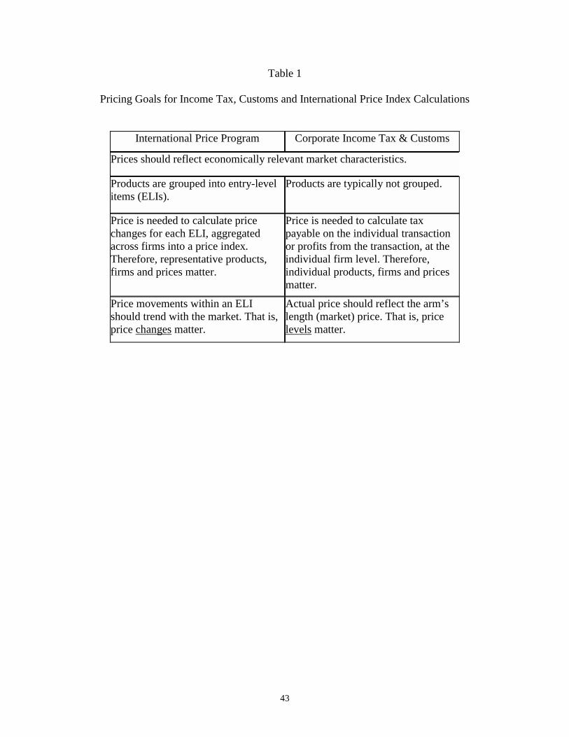
43

Table 1

Pricing Goals for Income Tax, Customs and International Price Index Calculations

International Price Program Corporate Income Tax & Customs

Prices should reflect economically relevant market characteristics.

Products are grouped into entry-level items (ELIs).

Products are typically not grouped.

Price is needed to calculate price changes for each ELI, aggregated across firms into a price index. Therefore, representative products, firms and prices matter.

Price is needed to calculate tax payable on the individual transaction or profits from the transaction, at the individual firm level. Therefore, individual products, firms and prices matter.

Price movements within an ELI should trend with the market. That is, price changes matter.

Actual price should reflect the arm’s length (market) price. That is, price levels matter.

44

References Alterman, W. F., W. E. Diewert and R. C. Feenstra, (1999), International Trade Price Indexes

and Seasonal Commodities, Bureau of Labor Statistics, Washington D.C. Archibald, R. B. (1977), “On the Theory of Industrial Price Measurement: Output Price

Indexes”, Annals of Economic and Social Measurement 6, 57-72. Bureau of the Census (2002), “U.S. Goods Trade: Imports and Exports by Related Parties;

2001”, United States Department of Commerce News, Economics and Statistics Information, Bureau of the Census: Washington DC, 20230. Website: http://www.census.gov/foreign-trade/Press-Release/2001pr/aip/rp01.pdf

Clausing, K. A. (2001), “The Behavior of Intrafirm Trade Prices in U. S. International Price

Data”, BLS Working Paper 333, Washington DC: U. S. Department of Labor, Bureau of Labor Statistics, January. Website: http://stats.bls.gov/ore/pdf/ec010010.pdf

Copithorne, L. (1976), “La théorie des prix des transfert internes des grandes sociétés”,

L’actualité économique 52, 324-352. Deloitte and Touche (2002), “Advanced Pricing Agreements”. Website:

http://deloitte.com/dtt/cda/doc/content/APA.pdf Diewert, W. E. (1974), “Applications of Duality Theory”, pp. 106-171 in Frontiers of

Quantitative Economics, Volume II, M. Intriligator and D. Kendrick (eds.), Amsterdam: North-Holland.

Diewert, W. E. (1980), “Aggregation Problems in the Measurement of Capital”, pp. 433-528 in

The Measurement of Capital, Dan Usher (ed.), University of Chicago Press, Chicago. Diewert, W. E. (1983), “The Theory of the Output Price Index and the Measurement of Real

Output Change”, pp. 1049-1113 in Price Level Measurement, W. E. Diewert and C. Montmarquette (eds.), Ottawa: Statistics Canada.

Diewert, W. E. (1985), “Transfer Pricing and Economic Efficiency”, pp. 47-81 in Multinationals

and Transfer Pricing, A. M. Rugman and L. Eden (eds.), London: Croom Helm. Diewert, W. E. (1993), “Duality Approaches to Microeconomic Theory”, pp. 105-175 in Essays

in Index Number Theory, Volume 1, W. E. Diewert and A. O. Nakamura (eds.), Amsterdam: North-Holland.

Diewert, W. E. (2002), “Harmonized Indexes of Consumer Prices: Their Conceptual

Foundations”, Working Paper No. 130, European Central Bank, Kaiserstrasse 29, D-60311 Frankfurt am Main, Germany.

Dorgan, B. (2002), “Dorgan Releases Study that Shows Multinational Corporations use Phony

45

Pricing Schemes to Avoid $53.1 Billion in U. S. Taxes”, News Release, November 1, Byron Dorgan, U. S. Senator, North Dakota, 713 Hart Senate Office Building, Washington DC, 20510. Website: http://dorgan.senate.gov/newsroom/record.cfm?id=187978

Eden, L. (1985) “The Microeconomics of Transfer Pricing”, pp. 13-46 in Multinationals and

Transfer Pricing, A. M. Rugman and L. Eden (eds.), London: Croom Helm. Eden, L. (1998), Taxing Multinationals: Transfer Pricing and Corporate Income Taxation in North America, Toronto: University of Toronto Press. Eden, L. (2001a), International Taxation, Transfer Pricing and the Multinational Enterprise. In

The Oxford Handbook of International Business, edited by Alan Rugman and Thomas Brewer. London, UK: Oxford University Press, pp. 591-619.

Eden, L. (2001b), “Transfer Pricing, Intrafirm Trade and the BLS International Price Program”,

BLS Working Paper 334, Washington DC: U. S. Department of Labor, Bureau of Labor Statistics, January. Website: http://stats.bls.gov/ore/pdf/ec010020.pdf

Eden, L. and P. Rodriguez (2004), How Weak Are the Signals? International Price Indices and

Multinational Enterprises. Journal of International Business Studies, 35.1: 61-74. Ernst & Young (2001), Transfer Pricing 2001 Global Survey: Making Informed Decisions in

Uncertain Times: Practices, Perceptions and Trends in 22 Countries, Ernst and Young International. Website: http://www.ey.com/global/download.nsf/Denmark/TP_2001_Global_Survey/$file/2001_Global_TP_Survey_final.pdf

Ernst & Young (2003), Transfer Pricing 2003 Global Survey: Practices, Perceptions and

Trends in 22 Countries Plus Tax Authority Approaches in 44 Countries. Website: http://www.ey.com/GLOBAL/content.nsf/International/Transfer_Pricing_2003_Global_Survey

Feinschreiber, R. (2004), Transfer Pricing Methods: An Applications Guide, New York: John

Wiley & Sons, Inc. Fisher, F. M. and K. Shell (1972), “The Pure Theory of the National Output Deflator”, pp. 49-

113 in The Economic Theory of Price Indexes, New York: Academic Press. Freedman, D. (2002), “Running Away from Taxes: Senator Grassley Fights Offshore Evaders”,

The Miami Herald, December 23. Website: http://www.miami.com/mld/miamiherald/business/4787109.htm

Frisch, R. (1936), “Annual Survey of General Economic Theory: The Problem of Index

Numbers”, Econometrica 4, 1-39.

46

Hirshleifer, J. (1956), “On the Economics of Transfer Pricing”, Journal of Business 29, 172-183. Internal Revenue Service (2002), “Announcement and Report Concerning Advance Pricing

Agreements”, Department of the Treasury, Washington DC, March 29. Website: http://www.irs.gov/pub/irs-apa/apa_report_2002_40.pdf

Mozes, S. and D. Oberg (2002), “U. S.-Canada Data Exchange: 1990-2001”, U. S. Census

Bureau, Washington D.C. Website: http://www.census.gov/foreign-trade/aip/uscanada.pdf

OECD (1995) Transfer Pricing Guidelines for Multinational Enterprises and Tax

Administrations. Paris: OECD. Pak, S. J. and J. S. Zdanowicz (2002), “U. S. Trade with the World: An Estimate of 2001 Lost U.

S. Federal Income Tax Revenues due to Over-Invoiced Imports and Under-Invoiced Exports”, Executive Summary to the U. S. Senate, October 31, 2002. Website: http://dorgan.senate.gov/newsroom/extras/pak-zdan.pdf

Samuelson, P. A. (1947), Foundations of Economic Analysis, Cambridge MA: Harvard

University Press. Samuelson, P. A. and S. Swamy (1974), “Invariant Economic Index Numbers and Canonical

Duality: Survey and Synthesis”, American Economic Review 64, 566-593. Schulman, Ronca and Bucuvalas, Inc. (2001), “IRS Contemporaneous Documentation Survey:

Final Report”, December 11. Website: http://www.irs.gov/pub/irs-utl/report_121101.pdf U.S. General Accounting Office, (2000), Tax Administration: IRS’ Advance Pricing Agreement

Program, GAO/GGD-00-168. Washington, DC: General Accounting Office, August. Zeile, W. J. (1997), “US Intrafirm Trade in Goods”, Survey of Current Business 77 (February),

23-38. Website: http://www.bea.gov/bea/ARTICLES/INTERNAT/BPA/1997/0297iid.pdf