impact of free trade agreement use on import prices

Policy Research Working Paper 8416

Impact of Free Trade Agreement Use on Import Prices

Kazunobu HayakawaNuttawut Laksanapanyakul

Hiroshi MukunokiShujiro Urata

Development Economics Vice PresidencyStrategy and Operations TeamApril 2018

WPS8416P

ublic

Dis

clos

ure

Aut

horiz

edP

ublic

Dis

clos

ure

Aut

horiz

edP

ublic

Dis

clos

ure

Aut

horiz

edP

ublic

Dis

clos

ure

Aut

horiz

ed

Produced by the Research Support Team

Abstract

The Policy Research Working Paper Series disseminates the findings of work in progress to encourage the exchange of ideas about development issues. An objective of the series is to get the findings out quickly, even if the presentations are less than fully polished. The papers carry the names of the authors and should be cited accordingly. The findings, interpretations, and conclusions expressed in this paper are entirely those of the authors. They do not necessarily represent the views of the International Bank for Reconstruction and Development/World Bank and its affiliated organizations, or those of the Executive Directors of the World Bank or the governments they represent.

Policy Research Working Paper 4816

This paper is a product of the Strategy and Operations Team, Development Economics Vice Presidency. It is part of a larger effort by the World Bank to provide open access to its research and make a contribution to development policy discussions around the world. Policy Research Working Papers are also posted on the Web at http://www.worldbank.org/research. The authors may be contacted at [email protected].

This paper examines the impact of free trade agreement (FTA) use on import prices. For this analysis, it employs establishment-level import data with information on tariff schemes, that is, the FTA and most-favored-nation schemes used for importing. Unlike previous studies, this paper estimates the effects of FTA use on prices by controlling for differences in importing-firm characteristics. There are

three main findings. First, the effect of FTA use is overes-timated when not controlling for importing firm-related fixed effects. Second, on average, firms’ FTA use reduces tariffs by 12 percentage points and raises import prices by 3.6–6.7 percent. Third, in general, a price rise resulting from the costs of complying with rules of origin was not found.

Impact of Free Trade Agreement Use on Import Prices

Kazunobu Hayakawa, Nuttawut Laksanapanyakul, Hiroshi Mukunoki, and Shujiro Urata

JEL classification: F15, F53

Key words: Free trade agreement, Thailand, Tariffs

Kazunobu Hayakawa (corresponding author) is a senior research fellow at the Institute of Developing Economies, Japan; his

email address is [email protected]. Nuttawut Laksanapanyakul is a researcher at Thailand Development

Research Institute, Thailand; his email address is [email protected]. Hiroshi Mukunoki is a professor at Gakushuin

University, Japan; his email address is [email protected]. Shujiro Urata is a professor at Waseda

University, Japan; his email address is [email protected]. This research was conducted as part of a project by the Economic

Research Institute for ASEAN and East Asia, “Comprehensive Analysis on Free Trade Agreements in East Asia.” We would

like to thank Luis Servén (Associate Editor of this journal), two anonymous referees, Fukunari Kimura, Kiyoyasu Tanaka,

Toshiyuki Matsuura, Kozo Kiyota, Taiyo Yoshimi, and the seminar participants at Chukyo University, the Japan Society of

International Economics, and the East Asian Economic Association. This work was supported by JSPS KAKENHI Grant

Number 26705002.

2

Trade liberalization yields various economic impacts. One of the impacts is to lower the consumer

prices of imported products through the reduction in tariffs, which benefits consumers and improves

welfare in importing countries. Lower consumer prices can also contribute to reducing poverty (e.g.,

Broda, Leibtag, and Weinstein 2009). Meanwhile, the rise in (tariff-exclusive) trade prices amplifies the

exporting country’s benefits by increasing the value of exports and thus exporters’ profits. In addition

to these benefits, as suggested by Melitz (2003) and Kasahara and Lapham (2013), trade liberalization

promotes resource reallocation both across industries and within each industry, thus improving

macro-level productivity.

Over recent decades, the principal way of advancing trade liberalization has shifted from

multilateral agreements to preferential agreements. Tariff reductions have been implemented under

the most-favored-nation (MFN) principle, which is the backbone of policy discipline for the General

Agreement on Tariffs and Trade (GATT) and the World Trade Organization (WTO). Tariff reductions

under the WTO, however, have not advanced well in the Doha Development Agenda. As a result, most

countries have started to aggressively exploit “exceptions” to the MFN principle, of which a typical form

is the free trade agreement (FTA). By July 2017, more than 400 FTAs had been notified to the GATT and

the WTO.

An important policy question in this shift is the extent of the differences in the economic impacts

of trade liberalization under FTAs and the MFN principle. One of the key differences between these two

3

types of liberalization is that exporters must comply with rules of origin (RoO) to use an FTA and to

benefit from preferential FTA tariffs. Products exported under FTAs need to originate from FTA

member countries. FTAs may induce exporters to change their procurement sources and raise material

costs. To certify the “origin” of their products, they must submit various documents, such as invoices

for each input. To handle this, exporters may establish an administrative division or assign staff to be in

charge of FTA use. Because of these additional costs, unlike the case of trade liberalization under MFN,

some firms cannot benefit from trade liberalization under FTA. These costs may diminish the gains

from liberalization for FTA users and change the distribution of gains between exporters and

importers.

Among the many impacts of trade liberalization, this study sheds light on the effects of firms’ FTA

use on their trade prices.1,2 There exist channels for such price changes resulting from FTA use. The

traditional channel is based on the change in markup due to the use of FTA preferential rates, which are

lower than MFN rates. As summarized in Feenstra (2003), under some conditions, a reduction in tariff

rates raises export prices. We call this effect the “tariff effect.” Another possible channel is the increase

1 We use the following expressions interchangeably: trade price, export price, and import price.

2 General changes to trade prices caused by tariff rates are called the “tariff pass-through.” Feenstra (1989)

was one of the early studies on tariff pass-through, although he did not examine tariff changes under FTAs.

Gorg, Halpern, and Muraközy (2010) examined the tariff pass-through for Hungarian exports at the firm level

but did not find significant tariff pass-through. By contrast, Ludema and Yu (2016) found significant firm-level

tariff pass-through in US exports.

4

in production costs due to the above-mentioned RoO compliance. We call this the “RoO effect.” We

examine the tariff and RoO effects separately. Separate examination such as this is important once one

realizes that a simple reduction in MFN rates yields the tariff effect but not the RoO effect. In addition,

other channels may exist. To compensate for the costs of using FTAs, potential FTA exporters may

bargain over export prices with importers.

Several studies have empirically quantified the overall effects of FTAs on trade prices without

differentiating between tariff and RoO effects. Most of these studies employ product-level import data

to differentiate trade values according to tariff scheme. Cadot et al. (2005) found a rise in export prices

in the context of Mexican textile and apparel exporters through use of the North American FTA

(NAFTA) of around 80 percent of the tariff margin (the difference between the FTA and MFN rates).

Ozden and Sharma (2006) examined the impact of the United States’ Caribbean Basin Initiative on the

prices received by eligible apparel exporters and found that export prices rose by around 65 percent of

the tariff margin. African apparel exporters captured 16–53 percent of the tariff margin under the

African Growth and Opportunity Act (Olarreaga and Ozden 2005). Cirera (2014) found the rise in

export prices to the European Union through the use of the generalized scheme of preferences and its

related schemes to be 17–80 percent of the tariff margin. Overall, previous studies using product-level

data have found higher export prices for exporters trading under FTA schemes than under MFN

schemes.

5

The difference in export prices may reflect not only the use of different tariff schemes but also the

characteristics of the firms. Not all firms can necessarily benefit from trade liberalization under FTAs.

Demidova and Krishna (2008) theoretically demonstrated that exporters under MFN and FTA schemes

are systemically different in terms of productivity.3 For example, if productive firms have lower export

prices owing to having lower marginal costs and are likely to use FTA schemes when exporting, then

the export prices under FTA schemes will be related not only to the effects of FTA use but also to the

effect of the exporter’s productivity. Besides these exporter characteristics, importer characteristics

may affect the use of FTA schemes in trading and yield biased estimates of the effects of FTAs on export

prices. Obtaining unbiased estimates of the effects of FTAs on export prices requires the consideration

of firm-level factors. To the best of our knowledge, no studies have thus far addressed these problems

successfully.

3 Demidova and Krishna (2008) introduced choice of tariff schemes into Melitz’s (2003) firm-heterogeneity

model.

6

To examine the effects of FTA use on import prices, we employ transaction-level import data for

Thailand during 2007–2011.4,5 This dataset enables us to identify not only the date of import, firm,

branch, exporting country, and commodity (at the 2007 harmonized system [HS] eight-digit level) but

also the tariff scheme (e.g., FTA scheme or MFN scheme) used by the importing firm and branch.6 We

focus on the effects of using the FTA by the Republic of Korea (henceforth Korea) in the ASEAN–Korea

FTA (AKFTA). During 2007–2011, Thailand had bilateral and/or plurilateral FTAs with 15 countries.7

One of the main reasons for selecting the AKFTA is that it entered into force in the middle of our sample

period, in 2010. Further, the FTA entered into force at a time that was unpredictable for firms in

Thailand because of exogenous events such as the political turmoil. These features enhance the validity

of our empirical identification of the effects of FTA use. Another reason for selecting the AKFTA is that

4 In general, the use of exporter-side data in the FTA literature has some problems. For example, data on FTA

use for exports are difficult to obtain in the case of FTAs adopting the self-certification system. For more details,

see Hayakawa et al. (2013a).

5 This period includes the global financial crisis in 2007/2008. In the estimation section, we address this issue

to some extent.

6 Although several recent empirical studies have used firm-level trade data (e.g., Amiti, Itskhoki, and Konings

2014; Berman, Martin, and Mayer 2012; Eaton, Kortum, and Kramarz 2011), few have used data that

enable identification of tariff schemes. One exception is Cherkashin et al. (2015); however, their dataset

covered only the apparel industry, whereas our dataset covers all sectors.

7 These countries are Australia, China, Japan, Korea, India, New Zealand, the Philippines, Brunei Darussalam,

Cambodia, Lao PDR, Myanmar, Malaysia, Indonesia, Singapore, and Vietnam.

7

we can avoid examining complex decisions by firms vis-à-vis tariff schemes. Most of the FTAs enacted

by Thailand have overlap in country coverage. Thailand has not only bilateral but also plurilateral FTAs

with Japan, Australia, New Zealand, and India. When multiple FTA schemes are available, firms’ choice

of tariff scheme becomes complicated. To avoid this complication, we focus on imports from Korea,

which has a single FTA scheme with Thailand.

We examine the effects of FTA use by controlling for various fixed effects. To do so, our sample

includes imports from not only Korea but also countries with which Thailand does not have an FTA. We

estimate the import price equations at the importing establishment level rather than at the importing

firm level. Since this method yields more variation across the observations within a given importing

firm, it is easy to control for importing-firm characteristics. We can examine how import prices change

for the same establishment before and after AKFTA by controlling for time-variant importing-firm fixed

effects in addition to importing establishment-exporting country-product fixed effects and time-

variant-exporting country-sector fixed effects. Our estimates are less biased compared with those

obtained in previous studies.

By using these strategies, we empirically examine the effects of FTA use on import prices. We first

simply regress import prices on an FTA use dummy to assess how the results change when we control

for various importing firm-related fixed effects and thus uncover the existence of biases in the

estimates found in previous studies. Then, we examine the tariff and RoO effects separately. We further

8

conduct analyses by considering various important factors. We control for the effects of tariff reduction

on the quality of imported products. There is a growing literature on the trade price–quality nexus.8

Focusing on China, Bas and Strauss-Khan (2015) empirically established that a reduction in MFN rates

allows firms to upgrade the quality of their imported inputs, resulting in a rise in import prices. FTA

use may also encourage import firms to change trade partners in favor of those who produce higher-

quality products. Since our interest does not lie in that domain, we estimate our model for observations

with little change in the quality of imported products.

The rest of this paper is organized as follows. In Section 1, we theoretically demonstrate how FTA

use affects import prices, focusing particularly on the tariff and RoO effects. After specifying our

empirical framework in Section 2, we report our estimation results in Section 3. Finally, Section 4

concludes the paper.

I. Theoretical Framework

This section explains the theoretical background of our estimation. We first set up our model.

Specifically, we consider a monopolistic competition model where products are differentiated within

the same product category. Then, we examine how tariff reduction and RoO compliance through FTA

8 Examples include Khandelwal (2010), Amiti and Khandelwal (2013), Khandelwal et al. (2013), Bas and

Strauss-Khan (2015), and Fan, Li, and Yeaple (2015).

9

use change import prices. Finally, to demonstrate that the choice of FTA schemes is not random across

firms, we consider the selection of tariff schemes by exporters.

Basic Setup

Consider an economy with L consumers who have symmetric preferences over a continuum of

imported varieties of products supplied within the same product category. The utility of each consumer

is given by

Ω ( ) ,i

iU u c di

(1)

where 𝑐𝑖 is each individual’s consumption of product variety i and Ω is the set of available product

varieties. We assume 𝑢(0) = 0, 𝑢′(𝑐𝑖) > 0, and 𝑢′′(𝑐𝑖) < 0 for 𝑐𝑖 > 0. Each consumer supplies one unit of

labor and earns 𝑤. Without loss of generality, we set 𝑤 = 1. Let 𝑝𝑖 denote the consumer price of

product variety i. Consumers individually maximize U subject to Ω

1i ii

p c di

. From the first-order

condition, inverse individual demand becomes

𝑝𝑖 (𝑐𝑖) =𝑢′(𝑐𝑖)

𝜆 , (2)

where Ω

'( )i ii

u c c di

is the marginal utility of income. We can calculate the price elasticity of

individual demand as

휀𝑖 (𝑐𝑖) = −𝑝𝑖(𝑐𝑖)

𝑝𝑖′(𝑐𝑖)𝑐𝑖= −

𝑢′(𝑐𝑖)

𝑢′′(𝑐𝑖)𝑐𝑖. (3)

10

The elasticity needs to satisfy 휀𝑖(𝑐𝑖) > 1 to derive the equilibrium price. Under a constant

elasticity of substitution preferences, which are often assumed for tractability in monopolistic

competition models, the price elasticity of demand is constant and does not depend on 𝑐𝑖 . Under

constant price elasticity, however, a tariff reduction does not affect the import price, as we see below.

We thus need a variable price elasticity of demand to examine how a tariff reduction affects the import

price.

Here, we focus on imported product varieties. Since demand is symmetric for all imported

product varieties, we drop the variety index hereafter. The (tariff-exclusive) import price is denoted by

𝑝𝑖𝑚𝑝. Let 𝑇 ∈ {𝑇𝐹𝑇𝐴, 𝑇𝑀𝐹𝑁} be the ad valorem tariff imposed on the imports. Then, we have

𝑝 = (1 + 𝑇)𝑝𝑖𝑚𝑝. The tariff under the FTA scheme should be lower than the tariff under the MFN

scheme: 𝑇𝐹𝑇𝐴 < 𝑇𝑀𝐹𝑁. If the firm uses the FTA scheme, however, it must incur the fixed

documentation cost to certify the origin of products, which is given by F.

Because consumers are symmetric, the production of each product variety is the sum of their

individual consumption and is given by 𝑞 = 𝑐𝐿. Let θ denote a parameter that takes 𝜃 = 1 if the firm

uses the FTA or 𝜃 = 0 if it chooses the MFN tariff. Then, the tariff level that the firm faces is given by

𝑇 (𝜃) = 𝜃𝑇𝐹𝑇𝐴 + (1 − 𝜃)𝑇𝑀𝐹𝑁. The marginal cost of the firm is given by Γ (𝜃) = {𝜃𝛿 + (1 − 𝜃)}𝛾,

where γ is the firm-specific unit cost of production (i.e., the inverse of firm productivity). To comply

with the RoO, firms may need to adjust their procurement sources. We capture the degree of an

11

increase in the unit cost for such a procurement adjustment by δ (≥1). Note that 𝛿 = 1 if the firm’s

procurement under the MFN scheme meets RoO. The operating profit of the firm (i.e., the profit before

subtracting the fixed cost) in a foreign country that produces each variety is given by

𝜋 (𝑞, 𝜃) = [𝑝(𝑞 𝐿⁄ )

1+𝑇(𝜃)− Γ(𝜃)] 𝑞. (4)

We follow the standard model of monopolistic competition and assume that the number of

varieties is sufficiently large. Then, firms regard the level of λ as given. The firm maximizes profit with

respect to q. From the first-order condition of profit maximization, the optimal level of production, �̃�,

is determined to satisfy

𝜕𝜋(�̃�,𝜃)

𝜕𝑞=

𝑝(�̃� 𝐿⁄ )

1+𝑇(𝜃) [1 −

1

(�̃� 𝐿⁄ )] − Γ (𝜃) = 0. (5)

Accordingly, the equilibrium level of individual consumption and equilibrium consumer price

respectively become �̃� = �̃� 𝐿⁄ and �̃� = 𝑝(�̃�). The second-order condition of profit maximization

requires

𝜕2𝜋(�̃�,𝜃)

(𝜕𝑞)2 = −𝑝(𝑐){2−𝜂(𝑐)}

{1+𝑇(𝜃)}𝑞 (𝑐)< 0, (6)

where 𝜂 (𝑐) = −𝑐𝑝′′(𝑐)/𝑝′(𝑐) is the elasticity of the slope of the inverse demand function. The

demand curve is concave if 𝜂(𝑐) ≤ 0 and convex if 𝜂(𝑐) > 0. To satisfy (6), 2 > 𝜂(𝑐) must hold. By

rearranging (5), the equilibrium import price of each variety is given by

�̃�𝑖𝑚𝑝 =�̃�

1+𝑇(𝜃) = 𝑚(�̃�)Γ(𝜃), (7)

12

where 𝑚 (𝑐) = 휀(𝑐) {휀(𝑐) − 1} > 1⁄ is (one plus) the markup over the marginal cost.

Effects of FTA Use on Import Prices

An ad valorem tariff does not directly affect �̃�𝑖𝑚𝑝, but it may indirectly change �̃�𝑖𝑚𝑝 because it

increases the consumer price, �̃�. Specifically, an increase in �̃� decreases �̃� and thereby changes 휀(𝑐)

and the price–cost markup. By differentiating (5) with respect to 1 + 𝑇(𝜃) and Γ(𝜃), we have

𝑑 ln 𝑐̃

𝑑 ln{1+𝑇(𝜃)}=

𝑑 ln 𝑐̃

𝑑 ln Γ(𝜃) = −

(𝑐̃)−1

2−𝜂(𝑐̃)< 0. (8)

An increase in 𝑇(𝜃) or Γ(𝜃) reduces the individual consumption of the variety. Then, the effect

of an increase in a tariff on the import price is given by

𝑑 ln �̃�𝑖𝑚𝑝

𝑑 ln{1+𝑇(𝜃)}=

𝑑 ln 𝑚(𝑐̃)

𝑑 ln 𝑐̃

𝑑 ln 𝑐̃

𝑑 ln{1+𝑇(𝜃)}. (9)

Hence, whether an import tariff increases or decreases the import price depends on the sign of

𝑑 ln 𝑚(�̃�)/(𝑑 ln �̃�), that is, on how a change in �̃� affects the price–cost markup. If 𝑑 ln 𝑚(�̃�)/(𝑑 ln �̃�) >

0, then 𝑑 ln �̃�𝑖𝑚𝑝 [𝑑 ln{1 + 𝑇(𝜃)}] < 0⁄ holds. In this case, a lower consumer price and an increase in

consumption induced by the tariff reduction raise the markup and import price. If 𝑑 ln 𝑚(�̃�)/(𝑑 ln �̃�) <

0, however, the tariff reduction lowers both the consumer price and the import price. If

𝑑 ln 𝑚(�̃�)/(𝑑 ln �̃�) = 0, in other words, if consumer preferences follow a constant elasticity of

substitution function, then the tariff reduction lowers the consumer price but the import price remains

unchanged.

13

More specifically, we have

𝑑 ln 𝑚(𝑐)̃

𝑑 ln 𝑐̃=

�̂�−𝜂(𝑐̃)

(𝑐̃)−1 . (10)

Therefore, 𝑑 ln 𝑚(�̃�)/(𝑑 ln �̃�) > 0 holds if the elasticity of the slope of the inverse demand is low

to satisfy 𝜂(�̃�) < �̂� ≡ 1 + 1/휀(�̃�). A tariff reduction lowers the consumer price and increases the

equilibrium consumption, and the increased consumption decreases the price elasticity of demand

(i.e., 휀′(�̃�) < 0) unless the demand curve is highly convex. The decreased price elasticity of demand in

turn increases the price–cost markup because consumers become less sensitive to price changes. In

addition, by substituting (8) and (10) into (9), we have


𝑑 ln{1+𝑇(𝜃)}= −

�̂�−𝜂(𝑐̃)

2−𝜂(𝑐̃). (11)

A larger 𝜂(�̃�) diminishes the price-increasing effect of the tariff reduction.

Note that the decreasing price elasticity of demand is not specific to our specification of the

model. Krugman (1979) assumed decreasing price elasticity in his seminal paper on intra-industry

trade. Bertoletti and Epifani (2014) and Kichko, Kokovin, and Zhelobodko (2014) showed that a

decreasing elasticity of substitution in the utility function yields 휀′(�̃�) < 0. Decreasing price elasticities

were also obtained by Melitz and Ottaviano (2008) with a linear demand function and by Behrens and

Murata (2007) with additively quasi-separable functions.

14

We have examined how changes in the import tariff affect the import price. Next, we examine the

effect of an increase in the marginal cost, Γ(𝜃), on the equilibrium import price. We have


𝑑 ln Γ(𝜃)= 1 +

𝑑 ln 𝑚(𝑐̃)

𝑑 ln 𝑐̃

𝑑 ln 𝑐̃

𝑑 ln Γ(𝜃)=

1

𝑚(𝑐̃){2−𝜂(𝑐̃)} > 0. (12)

Hence, a higher marginal cost of a firm always leads to a higher import price. Note that a larger

𝜂(�̃�) increases the price-increasing effect of the marginal cost. As a result, we have the following

proposition.

Proposition 1 A reduction in the tariff increases the import price if the elasticity of the slope of the

inverse demand function is low (𝜂(�̃�) < �̂�). It decreases the import price if the elasticity is high

(𝜂(�̃�) > �̂�) and does not affect the import price if the elasticity is equal to the threshold (𝜂 (�̃�) =

�̂� ). An increase in the marginal cost always increases the import price.

Proposition 1 provides an important implication for the impact of FTA use on import prices. By

using an FTA scheme, a firm, on the one hand, faces an FTA tariff that is lower than the MFN tariff (the

tariff effect). On the other hand, the firm must incur the costs of meeting the RoO, part of which

increases the marginal cost of the firm and thus the import price (the RoO effect). If the elasticity of the

slope of the demand curve is low, the tariff effect increases the import price. If the elasticity is high,

however, the tariff effect increases the import price less or may even decrease the import price,

whereas the RoO effect always increases the import price irrespective of the curvature of the demand

curve. This fact implies that if FTA use increases the import price, the increased markup is the main

driving force if the elasticity of the slope of the demand curve is low (𝜂(�̃�) < �̂�), whereas the RoO effect

15

plays an important role otherwise (𝜂(�̃�) ≥ �̂�). Put differently, if the RoO effect is not so significant,

then the firm gains more and consumers gain less from FTA use in the former case, whereas a large

part of the gains accrues to consumers in the latter case.

We have shown that several exogenous parameters govern the equilibrium import price.

However, we cannot explicitly solve the equilibrium import price from (7), because the price elasticity

of demand that affects �̃�𝑖𝑚𝑝 is not constant and varies with �̃�, which recursively depends on the level

of �̃�𝑖𝑚𝑝. Hence, we implicitly define the import price function as

�̃�𝑖𝑚𝑝 = 𝑓(𝑇(𝜃), Γ(𝜃), 𝐿). (13)

The effects of Γ(𝜃) on the import price are positive, whereas those of 𝑇(𝜃) and L depend on the

shape of the demand curve. If the elasticity of the slope of the demand curve satisfies �̂� > 𝜂(�̃�), 𝑇(𝜃)

and L have negative impacts on �̃�𝑖𝑚𝑝. If the demand curve is highly convex and satisfies 𝜂(�̃�) > �̂�,

𝑇(𝜃) and L have positive impacts on �̃�𝑖𝑚𝑝.9 This equation is estimated in the following empirical

sections.

Choice between FTA and MFN Schemes

9 An increase in L decreases �̃�. Therefore, it decreases the import price if 휀′(�̃�) < 0 and increases the

import price if 휀′(�̃�) > 0.

16

In this last subsection, we investigate a firm’s choice between an FTA scheme and an MFN

scheme. By substituting (7) into (4), the equilibrium operating profit of the firm is given by

�̃� (�̃�, 𝜃) = [𝑚(�̃�) − 1]Γ(𝜃)�̃�𝐿. (14)

By differentiating (14) with respect to �̃�, we have

𝑑 ln �̃�(𝑐̃,𝜃)

𝑑 ln 𝑐̃= 1 +

𝑚(𝑐̃)

𝑚(𝑐̃)−1 𝑑 ln 𝑚(𝑐̃)

𝑑 ln 𝑐̃= 𝑚(�̃�){2 − 𝜂(�̃�)} > 0. (15)

Then, by differentiating (14) with respect to Γ(𝜃), and using (10) and (15), we can confirm that an

increase in the marginal cost reduces the firm’s operating profit:

𝑑 ln �̃�(𝑐̃,𝜃)

𝑑 ln Γ(𝜃)= 1 +

𝑑 ln �̃�(𝑐̃,𝜃)

𝑑 ln 𝑐̃

𝑑 ln 𝑐̃

𝑑 ln Γ(𝜃)= −{휀(�̃�) − 1} < 0. (16)

Similarly, the effect of tariffs on profit is given by

𝑑 ln �̃�(𝑐̃,𝜃)

𝑑 ln{1+𝑇(𝜃)}=

𝑑 ln �̃�(𝑐̃,𝜃)

𝑑 ln 𝑐̃

𝑑 ln 𝑐̃

𝑑 ln{1+𝑇(𝜃)}= −휀(�̃�) < 0. (17)

On the basis of these derivatives, we discuss the situation under which the producer of each

product variety chooses an FTA scheme over an MFN scheme. If the producer chooses the FTA scheme,

θ=1 holds and the equilibrium price and the individual consumption are respectively denoted by 𝑝𝐹𝑇𝐴

and 𝑐𝐹𝑇𝐴. Similarly, if the producer chooses the MFN scheme, we have θ=0, and the equilibrium price

and the consumption are respectively denoted by 𝑝𝑀𝐹𝑁 and 𝑐𝑀𝐹𝑁. Substituting these prices and

consumption into (14) yields the operating profit in each scheme:

𝜋𝐹𝑇𝐴 ≡ �̃� (𝑐𝐹𝑇𝐴, 1) = (𝑝𝐹𝑇𝐴 − 𝛿𝛾) 𝑐𝐹𝑇𝐴𝐿 = {𝑚(𝑐𝐹𝑇𝐴) − 1}𝛿𝛾𝑐𝐹𝑇𝐴𝐿, (18)

17

𝜋𝑀𝐹𝑁 ≡ �̃� (𝑐𝑀𝐹𝑁 , 0) = (𝑝𝑀𝐹𝑁 − 𝛾) 𝑐𝑀𝐹𝑁𝐿 = {𝑚(𝑐𝑀𝐹𝑁) − 1}𝛾𝑐𝑀𝐹𝑁𝐿. (19)

The difference between 𝜋𝐹𝑇𝐴 and 𝜋𝑀𝐹𝑁 is given by Δ𝜋 ≡ 𝜋𝐹𝑇𝐴 − 𝜋𝑀𝐹𝑁.

First, we examine the tariff effect of FTA use on the profit. Suppose δ=1, that is, the RoO does not

raise the marginal cost and FTA use only lowers the applied tariff from 𝑇𝑀𝐹𝑁 to 𝑇𝐹𝑇𝐴. From (17), we

have Δ𝜋 > 0, meaning that the gain in the operating profit from using the FTA is positive with δ=1. Δ𝜋

becomes larger as the tariff margin, 𝑇𝑀𝐹𝑁 − 𝑇𝐹𝑇𝐴, becomes larger. If the gain is large enough to exceed

the fixed cost of FTA use, Δ𝜋 > 𝐹, then the firm chooses the FTA scheme over the MFN scheme.

Next, we discuss the RoO effect of FTA use. An increase in δ reduces 𝜋𝐹𝑇𝐴, but it does not affect

𝜋𝑀𝐹𝑁. From (16) and (18), we have

𝑑 ln Δ𝜋

𝑑 ln 𝛿=

𝜋𝐹𝑇𝐴

Δ𝜋

𝑑 ln 𝜋𝐹𝑇𝐴

𝑑 ln 𝛿= −

𝜋𝐹𝑇𝐴

Δ𝜋{휀(𝑐𝐹𝑇𝐴) − 1} < 0. (20)

Therefore, as the RoO becomes more stringent, firms are less likely to use the FTA scheme. In

addition, a larger F obviously discourages FTA use.

Finally, let us examine how a firm’s productivity affects FTA use. Equation (16) tells us that an

increase in γ reduces the firm’s profit. By comparing the effect of γ on 𝜋𝐹𝑇𝐴 and 𝜋𝑀𝐹𝑁, we have

𝑑 ln Δ𝜋

𝑑 ln 𝛾= −{휀(𝑐𝐹𝑇𝐴) − 1} +

𝜋𝑀𝐹𝑁

Δ𝜋{휀(𝑐𝑀𝐹𝑁) − 휀(𝑐𝐹𝑇𝐴)}. (21)

Given that Δ𝜋 > 0, the effect of γ on Δ𝜋 is always negative if 휀(𝑐𝐹𝑇𝐴) > 휀(𝑐𝑀𝐹𝑁) holds, that is, if

the elasticity of the slope of the demand curve is high (𝜂(�̃�) ≥ �̂�) and 휀′(�̃�) > 0 holds. However, if the

18

elasticity of the slope of the demand curve is low (i.e., �̂� > 𝜂(�̃�)), then the effect of γ on Δ𝜋 can be

positive if 휀(𝑐𝑀𝐹𝑁) − 휀(𝑐𝐹𝑇𝐴) is large and Δ𝜋 is small. Note that Δ𝜋 becomes larger as the tariff

margin becomes higher and the RoO less stringent. If 𝑑 ln Δ𝜋 (𝑑 ln 𝛾)⁄ < 0 holds, then firms with

higher productivity (i.e., lower γ) are more likely to choose the FTA scheme.

Intuitively, if the price elasticity of demand does not depend on consumption, then higher

productivity increases a firm’s gains from FTA use because the FTA increases exports more without

changing the export price. This effect is reflected in the first term of (21). From (16), however, the

profit effect of higher productivity is larger if the price elasticity is higher. If the use of the FTA

decreases the elasticity, 휀(𝑐𝐹𝑇𝐴) < 휀(𝑐𝑀𝐹𝑁), then higher productivity reduces the gains from FTA use

because it increases the volume of exports more under the MFN scheme. This effect is reflected in the

second term of (21). In this case, the relative magnitude of these two effects determines the

relationship between firms’ productivity and FTA use.

The following proposition summarizes the firm’s choice of tariff scheme.

Proposition 2 A firm is more willing to use an FTA scheme as the preference margin of using the

FTA (i.e., 𝑇𝑀𝐹𝑁 − 𝑇𝐹𝑇𝐴 > 0) becomes larger. However, the firm is more likely to choose the MFN

scheme if the costs of the RoO (F and δ) are high. It is ambiguous whether a firm with higher

productivity will tend to use an FTA. If the elasticity of the slope of the demand curve is high

(𝜂(�̃�) ≥ �̂�), the tariff margin is large, or the costs of meeting the RoO are small, then productive

firms are more likely to use the FTA scheme.

II. Empirical Framework

19

This section explains the empirical strategy adopted to examine the effects of FTA use on import

prices, as described in Proposition 1. We first introduce our equation to be estimated and our dataset,

and then we provide a brief overview of FTA use in our dataset.

Specification

Our main dataset comprises transaction-level import data for Thailand from 2007 to 2011,

obtained from the Customs Department of Thailand.10 The dataset covers imports of all commodities

for Thailand and contains data on the customs clearing dates, HS eight-digit codes, exporting countries,

importing-firm codes, firm-branch codes, invoicing currencies, tariff schemes (e.g., FTA or MFN), and

import values in Thai baht. We classify the tariff schemes into three categories: MFN schemes, FTA

schemes, and other schemes. Other schemes include imports under the schemes of bonded

warehouses, free zones, investment promotion, duty drawbacks under Section 19, and duty drawbacks

for re-exports. Although it is interesting to take into account the choice of these other schemes, we do

not include imports under such other schemes in our sample to keep our analysis simple.

During our sample period, Thailand had 10 FTAs, most of which overlap in country coverage.

Thailand had both bilateral and plurilateral FTAs with Japan, Australia, New Zealand, and India. With

other ASEAN members, Thailand had six plurilateral FTA schemes: the ASEAN FTA, ASEAN–Australia–

10 We have been given permission to use these confidential data for academic purposes only.

20

New Zealand FTA, ASEAN–China FTA, ASEAN–Japan Comprehensive Economic Partnership, AKFTA,

and ASEAN–India FTA. In this study, we define the following 15 countries as “FTA member countries”:

Australia, Brunei, Cambodia, China, India, Indonesia, Japan, Korea, Lao PDR, Malaysia, Myanmar, New

Zealand, the Philippines, Singapore, and Vietnam. Except for Korea, with which Thailand concluded an

FTA in 2010, all these countries have been FTA partner countries for Thailand since at least the

beginning of our sample period of 2007. Other countries are defined as “FTA non-member countries.”

One empirical issue that needs attention when examining the effects of FTA use on import prices

is that FTA use and import prices are simultaneously determined. In addition, as shown in Proposition

2, the selection of FTA use is not random. Therefore, our identification strategy is as follows. First, by

taking advantage of the nature of our transaction-level panel data, we conduct a difference-in-

differences (DID) analysis on the effects of FTA use on import prices. To do so, in addition to all FTA

non-member countries, we include only one FTA member country, Korea, as an exporting country. As

mentioned, the FTA with Korea was the only one to enter into force during our sample period (i.e., in

2010). Therefore, during 2007–2009, the sample firms could not use an FTA scheme, but some were

able to do so during 2010–2011.

Second, another advantage of focusing on the AKFTA is that firms at the time were unable to

accurately predict when the FTA would enter into force. The ASEAN countries and Korea began FTA

negotiations in 2003. However, there was serious political turmoil in Thailand in 2006. As a result,

21

proceedings with respect to various external economic policies, including FTA policy, stopped in

Thailand. Hence, the AKFTA was signed by Korea and ASEAN member states, with the exception of

Thailand, in 2006. The AKFTA entered into force for all other countries in either 2007 or 2008, but for

Thailand it was unclear when or whether the negotiations on the AKFTA would restart. The agreement

was finally signed in 2009 and entered into force in 2010. This unpredictable situation of the AKFTA for

Thailand due to exogenous shocks to firms may enhance our identification for the DID analysis.11

Third, we examine establishment-level import prices rather than firm-level import prices.12

Further, our sample’s exporting countries include FTA non-member countries.13 These two notable

characteristics of our dataset enable us to easily control for all time-variant importing-firm

characteristics (e.g., productivity) in addition to fixed effects with various dimensions. In other words,

we can completely control for importing firm-specific elements that affect both FTA use and import

11 Another advantage of focusing on the AKFTA is the ability to avoid firms’ complicated decisions on tariff

schemes, which arise under the existence of multiple FTA schemes.

12 Greater firm-level variation exists if we examine transaction-level import prices rather than the annual

average of import prices. The estimation results for the analysis at the transaction level are introduced in Section

3.3.

13 We also estimate our model for all exporting countries, including other FTA member countries. We

introduce the estimation results for this case in Section 3.3.

22

prices.14 We use the data on imports aggregated by importing firms, their branches, exporting

countries, HS eight-digit codes, tariff schemes, and years.

For the empirical analysis, we parameterize the import price equation specified in (13). In

particular, we assume that it can be log-linearized as follows:

ln 𝑝𝑓𝑏𝑐𝑝𝑡 = 𝛼𝜃𝑓𝑏𝑐𝑝𝑡 − 𝛽 ln(1 + 𝑇𝑓𝑏𝑐𝑝𝑡) + 𝑢𝑓𝑏𝑐𝑝 + 𝑢𝑓𝑡 + 𝑢𝑐𝑠𝑡 + 휀𝑓𝑏𝑐𝑝𝑡 , (22)

where

1 + 𝑇𝑓𝑏𝑐𝑝𝑡 = {1 + 𝑀𝐹𝑁𝑝𝑡 𝑖𝑓 𝜃𝑓𝑏𝑐𝑝𝑡 = 0

1 + 𝐹𝑇𝐴𝑝𝑡 𝑖𝑓 𝜃𝑓𝑏𝑐𝑝𝑡 = 1 . (23)

pfbcpt denotes the import price (average unit value) by branch b of firm f in Thailand for an HS

eight-digit product p from country c in year t. θfbcpt indicates the tariff scheme and takes the value of

one if an observation is based on an import under the AKFTA and zero otherwise (called the “FTA

dummy”). Tfbcpt is the tariff rate in Thailand, which differs according to the tariff scheme used for

importing. MFN and FTA are the MFN rates and AKFTA preferential rates, respectively. The coefficient

α captures the RoO effect (i.e., δ in Section 1), whereas the coefficient β is related to the tariff effect.

Specifically, the coefficient α indicates whether the rise in marginal costs for RoO compliance by Korean

14 Instead of a model that controls for firm-specific elements, we also estimate a model that takes into account

to some extent the decision on FTA use. The estimation results for this case are reported in Table S2.1 in the

supplemental appendix.

23

exporters is passed through to import prices. When an establishment starts to import product p under

the AKFTA in year t, the magnitude of the tariff effect can be expressed as15

−𝛽{ln(1 + 𝐹𝑇𝐴𝑝𝑡) − ln(1 + 𝑀𝐹𝑁𝑝𝑡−1)} > 0. (24)

As shown in Proposition 1, both coefficients are expected to be positively estimated, particularly

when the elasticity of the slope of the inverse demand curve is low.

As mentioned, we control for various elements. ufbcp are the time-invariant, importing

establishment-exporting country-product fixed effects, which control for the importing establishment-

product-specific inherent characteristics. In addition, these fixed effects control for the role of the RoO

complied with by firms in the exporting country (i.e., Korea) because the RoO differ by product but do

not change over time. uft are the time-variant firm fixed effects used to control for all time-variant

importing-firm characteristics, such as knowledge and productivity.16 ucst are the time-variant,

exporting country-sector fixed effects. We define sectors by their HS two-digit codes. The fixed effects

15 Note that MFN rates are unchanged in 99.98 percent of all observations during our sample period.

16 We use import firm-year fixed effects rather than import establishment-year fixed effects. One reason for

this choice is that a firm’s productivity or knowledge is shared among its establishments. The other is to

maintain sufficient variation among the observations. The introduction of import establishment-year fixed

effects forces us to drop import establishments that import only one product from only one country, although

the number of such establishments is small (0.2 percent of all observations). We also estimate the model by

using import establishment-year fixed effects later.

24

control for production factor prices (e.g., wages) in the exporting countries in addition to sector-level

demand (i.e., L in Section 1) or the degree of competition in the importing country (i.e., Thailand). We

expect that these various fixed effects control for elements that affect both import prices and the choice

of tariff scheme.17

Our specification controls for biases that were not controlled for in previous studies. The

estimates of product-level studies such as Cadot et al. (2005), Ozden and Sharma (2006), and Olarreaga

and Ozden (2005) include not only the effect of FTA use but also the differences in exporter and/or

importer characteristics between FTA users and non-users. Our inclusion of time-variant importing-

firm fixed effects controls for all importing-firm characteristics. Moreover, if importing firms do not

change their country-product-level trading partners frequently, our importing establishment-country-

product dummy variables will, to some extent, be able to control for exporting-firm characteristics (e.g.,

exporter productivity, 1/γ in Section 1).

The remaining noteworthy point is that some establishments import products from Korea under

both the MFN and the FTA schemes for a number of reasons. One is that firms may import from

different firms under different tariff schemes (e.g., a productive export firm under the FTA scheme and

17 We cannot control for region-sector-year fixed effects since location information is not available in our

dataset.

25

a less productive export firm under the MFN scheme). The other is that firms may decide on the tariff

scheme for each transaction and choose the FTA scheme for transactions with a large trade value.18

For such observations, in the estimation sample, we retain those importing under the FTA scheme but

drop those importing under the MFN scheme to control for exporter characteristics as much as possible

through our importing establishment (-product-country) fixed effects.19

Data Overview

Before reporting our estimation results, we provide an overview of AKFTA use. The AKFTA

entered into force for Thailand in 2010 (signed in October 2009). Under the agreement, tariffs were

reduced according to the category into which each product is classified: normal track products,

sensitive list products, and highly sensitive list products. Since a tariff reduction for products in the

sensitive and highly sensitive lists started in 2012, AKFTA preferential rates are available only for

18 Indeed, we find significant evidence that larger transactions are more likely to occur under FTA schemes.

The results are shown in table S2.2 in the supplemental appendix.

19 Suppose that establishment A imported a product from firms B and C under the MFN scheme in 2009, and

it again imported that product from firm B under the MFN scheme and from firm C under the FTA scheme in

2010, although our dataset does not enable us to explicitly identify whether firms B and C are different. In this

example, we drop the observation of importing under the MFN scheme in 2010 (i.e., that of importing from

firm B in 2010). Otherwise, our import establishment(-product-country) dummy variable would take the value

of 1 for two observations (i.e., two tariff schemes) in 2010. To focus on the impacts of changing from the MFN

to the FTA scheme, we drop observations of importing under the MFN scheme for establishments that import

products under both the MFN and the FTA schemes. As a result, 0.2 percent of the observations are dropped.

26

products placed in the normal track during our sample period after the enactment of the AKFTA (i.e.,

2010 and 2011). The eligibility and level of AKFTA preferential rates did not change in 2010 or 2011. In

both years, 70 percent of all tariff-line products (8,300 products) were eligible under the AKFTA. The

average preference margin, the difference between the FTA and MFN rates, for the eligible products

was approximately 12 percent. The median and maximum margins were 7 percent and 266 percent,

respectively. The most commonly applied RoO was for a “change in heading or regional value content, ”

accounting for 77 percent of all tariff-line products. Other rules with a non-trivial share (8 percent)

include “change in chapter or regional value content” and “wholly obtained.”20

Next, we provide a brief overview of Thai imports from Korea. Table 1 reports various statistics

on Thai imports from Korea. The left-hand panel shows statistics for products where the MFN and FTA

rates coincide in 2011, and the right-hand panel shows those for products where the FTA rate is lower

than the MFN rate in 2011. Since our sample FTA is a multilateral FTA (i.e., an FTA among Korea and 10

ASEAN member states) with accumulation rules, firms have incentives to use FTA schemes, even for

products where MFN and FTA rates coincide, as they can enjoy the benefits from accumulation. When

firms export their products to other AKFTA member countries such as Indonesia under the AKFTA by

20 More detailed statistics on the RoO and preference margin are provided in supplemental appendix S1.

27

using materials from Korea as inputs for their products, those materials are imported under the AKFTA

even if the MFN rate for those materials is zero (see Hayakawa, Laksanapanyakul, and Shiino 2013b).

In table 1, we focus on the right-hand panel and define the products for which the FTA rates are

lower than the MFN rates as “eligible products.” From the number of importing establishment-product

observations, we can see that the number of FTA users is small compared with the number of MFN

users and importers under other schemes. In particular, the number of MFN users is at least 10 times

larger than that of FTA users. However, total import values differ little between MFN and FTA users,

particularly in 2011. These observations imply that average imports at the importing establishment-

product level are much larger for FTA users than for MFN users, although they are not so different

between FTA users and importers under other schemes. FTA users exhibit nearly 10 times greater

average import values than MFN users. This pattern is likely to reflect qualitative differences in

importing-firm characteristics between FTA users and MFN users.

Table 2 reports changes in tariff schemes at the importing establishment-product level between

2007 and 2011. In the table, we restrict the sample products to those in which FTA rates were lower

than MFN rates in 2011. “Both” indicates observations for which an establishment imported a product

under both the FTA and MFN schemes. “None” comprises cases of no imports under the MFN and FTA

schemes, but it includes imports under other schemes. A large number of “only MFN” users started or

stopped importing. Each case accounts for more than 40 percent of the observations. A relatively large

28

number also started importing under only the FTA scheme. The number of observations that changed

from “MFN” to “only FTA” is the smallest, accounting for only 0.1 percent; this is even smaller than for

the case of “both.”

Table 3 reports the means and medians of the log-differences of importing establishment-

product-level changes in import prices (import unit values) from 2007 to 2011. In this table, we restrict

the sample to observations that existed in both 2007 and 2011 and that used the MFN scheme in 2007.

In the case of “both”, we calculate the price changes for the MFN and FTA schemes separately. The

“nominal” row shows a relatively large increase in import prices for observations that changed in

status to “only FTA.” The median also shows a positive change in observations that changed in status to

the FTA scheme under “both.” These results are unchanged when we deflate import prices by using the

commodity-level consumer price index (normalized to 1 in 2007) obtained from the Bureau of Trade

and Economic Indices (Ministry of Commerce) of Thailand. The results for real import price changes

are shown in the row titled “real.” In sum, a relatively large increase in import prices is observed for

products for which the status changed to importing under the FTA scheme, although the absolute

magnitude of the price rise is small.

III. Empirical Results

This section reports our estimation results concerning the effects of FTA use on import prices. We

first present our basic estimation results to indicate how the results change when we control for

29

various importing firm-related fixed effects. Then, we report the estimation results for equation (22).

Descriptive statistics are provided in table 4.

Basic Estimation

Before estimating equation (22), we examine the existence or magnitude of bias in the estimation

of the effects of FTA use on import prices when not controlling for importing firm-related

characteristics. To do so, we simply regress the log of import prices on the FTA dummy variable by

including only country-sector-year fixed effects. The estimation results are reported in column (I) of

table 5. As per previous studies, the coefficient for the FTA dummy is estimated to be significantly

positive at the product level, indicating that import prices were 12 percent higher in international

transactions under the FTA scheme than in those under the MFN scheme. Since the average FTA

preferential tariff margin over the MFN rates was 12 percentage points, FTA preferential tariff margins

were absorbed by the increase in import prices.

The result changes significantly when we control for importing firm-related fixed effects. Column

(II) shows results for the case where importing establishment-country-product fixed effects are

included. The coefficient for the FTA dummy is statistically insignificant, and its magnitude is greatly

reduced. When controlling for not only importing establishment-country-product fixed effects but also

importing firm-year fixed effects, the coefficient is estimated to be insignificant, as shown in column

(III), and its magnitude is further reduced. Our findings indicate that both the inherent characteristics

30

of importing firms and time-variant characteristics seemed to have resulted in the overestimation of

the FTA effect in previous studies.

Tariff and Rules of Origin Effects

We estimate equation (22) that decomposes the effects of FTA use into tariff and RoO effects.

Table 6 presents the results of the estimation, which control for importing establishment-exporting

country-product, importing firm-year, and exporting country-sector-year fixed effects. In column (I),

we include only the tariff rates, of which the coefficient is estimated to be significantly negative,

indicating that the tariff reduction resulting from FTA use raises import prices. This result is consistent

with theoretical expectations for the case of the inverse demand curve with low slope elasticity (𝜂(�̃�) <

�̂�), as is demonstrated in Section 1. Quantitatively, the average MFN and AKFTA rates among eligible

products are 12.8 percent and 0.8 percent, respectively. Therefore, based on equation (24), the tariff

effect contributes, on average, to raising import prices by 3.6 percent (=−0.737*(0.0034−0.0525)*100),

implying that approximately 30 percent (=100*3.6/12.0) of the tariff margin is allocated to exporters

owing to the tariff effect.

Column (II) of table 6 includes both the FTA dummy and the tariff rate, which respectively

capture the RoO and tariff effects. The coefficient for the tariff rate is again estimated to be significantly

negative. Its absolute magnitude rises sharply from 0.737 to 1.374. A similar calculation as per the

above indicates that, on average, the tariff effect raises import prices by 6.7 percent and that

31

approximately 56 percent of the tariff margin is captured by exporters. On the other hand, the

coefficient for the FTA dummy is estimated to be insignificant. These results indicate that on average

the effects of FTA use on import prices are mainly based on the tariff effect, not on the RoO effect. This

implies that the effects of tariff reduction on import prices may not be different between the cases

based on FTA enactment and on multilateral liberalization (i.e., tariff reduction on an MFN basis).

Although it is difficult to generalize the above result from the export from Korea to Thailand,

there are indeed two supporting lines of evidence regarding the insignificant effect of RoO in Korea’s

export. First, the share of domestic value-added is very high. For example, according to the “Survey of

Japanese-Affiliated Firms in Asia and Oceania” (henceforth “the Survey”) in 2012, administered by the

Japan External Trade Organization, the average shares of labor costs, local materials/inputs, and

miscellaneous expenses in Japanese affiliates in Korea are respectively 17 percent, 32 percent, and 19

percent out of total production costs. Therefore, domestic value-added occupies 68 percent, which is

much higher than the usual cutoff in RVC rules (i.e., 40 percent). Second, the Survey for 2011 reports

responses by Japanese affiliates in Korea to a range of problems when exporting under FTA schemes.21

Consistent with the above observation concerning the high share of domestic value-added, it shows

that the major problem is the time taken to obtain CoO rather than whether or not to comply with RoO.

21 The table is provided in supplemental appendix S3.

32

In short, RoO compliance does not appear to be a serious issue at least in Korea and does not have a

significant effect on prices.

Robustness Checks

We conduct some robustness checks to explore the validity of our results. As mentioned in the

introductory section, the extant literature suggests that the reduction in tariff rates resulting from FTA

enables firms to import products with higher quality and higher prices. Since our interest lies in the

price effect of markups and RoO compliance, we control for the quality effect. Following the modified

version of the method proposed by Khandelwal, Schott, and Wei (2013), we first decompose import

prices into their quality component and quality-adjusted prices (QaPrice). We estimate the following

for imports from Korea and FTA non-member countries during our sample period using the OLS

method:

ln 𝑞𝑓𝑏𝑐𝑝𝑡 + 𝜎𝑝 ln((1 + 𝑇𝑓𝑏𝑐𝑝𝑡) × 𝑝𝑓𝑏𝑐𝑝𝑡) = 𝑢𝑝 + 𝑢𝑐𝑡 + 𝜖𝑓𝑏𝑐𝑝𝑡 ,

where 𝑞𝑓𝑏𝑐𝑝𝑡 denotes an import quantity of product p by firm f’s establishment b from country c in

year t. 𝑢 indicates fixed effects. 𝜎𝑝 indicates the elasticity of substitution for product p in Thailand,

which is available at the HS three-digit level in Broda, Greenfield, and Weinstein (2006). Log-quality

(ln �̂�𝑓𝑏𝑐𝑝𝑡) is measured by

ln �̂�𝑓𝑏𝑐𝑝𝑡 = 𝜖�̂�𝑏𝑐𝑝𝑡 (𝜎𝑝 − 1)⁄ ,

where 𝜖�̂�𝑏𝑐𝑝𝑡 is a residual term. The log of quality-adjusted prices (QaPrice) is obtained as

33

ln 𝑝𝑓𝑏𝑐𝑝𝑡 − ln �̂�𝑓𝑏𝑐𝑝𝑡 .

We drop import establishment-export country-product pairs where the absolute magnitude of

quality change over the sample period is in the top 10 percent in all pairs. Our theoretical framework in

Section 1 examines the price change with the same trading partner before and after the use of FTA and

considers neither partner change nor quality change of imported inputs. Since our dataset does not

enable us to identify export firms, we cannot directly exclude observations with those kinds of change.

Therefore, to reduce the possibility of including such observations, we retain only the observations

exhibiting little quality change. With those observations, we estimate the model specified in (23) for the

log of quality-adjusted prices. The results are shown in table 7. Columns (I) and (III) show the results

for (log of) import prices, whereas those for (log of) quality-adjusted prices are reported in columns

(II) and (IV). Although no significant results are presented in the former cases, the latter cases show

results similar to those in table 6.22

22 We also estimate a model for the quality component and confirm that the coefficient for the FTA dummy is

insignificant, indicating that our sample does not include a non-trivial number of observations with large

changes in product quality through FTA use. In addition, we estimate the quality component and QaPrice

separately for all observations. We also conduct this separate estimation only for imports of intermediate

products. However, all these cases lead to insignificant FTA dummy variable coefficients.

34

Additional robustness checks are as follows.23 First, we estimate our model for imports from all

countries, including those from other FTA member countries. We obtain significant results for the FTA

dummy and the tariff rate when introducing the variables separately. Only the coefficient for the FTA

dummy is estimated to be significantly positive when introducing both variables simultaneously.

Second, we use transaction-level data rather than aggregated data according to year. Although the

coefficient for the FTA dummy is negative when introducing both variables, the results are similar to

those in the preliminary robustness check when introducing the two variables separately. Third, to

examine differences in the RoO effect across RoO, we introduce interaction terms for the FTA dummy

variable with various dummy variables indicating RoO. The results reveal that only the interaction term

incorporating the regional value content rule is significantly negative. This sign is not consistent with

our expectations. Furthermore, the absolute magnitude of the coefficient is abnormally large.24

23 The results are shown in tables S2.3–S2.5 in the supplemental appendix. In table S2.6, we also report

estimation results for the equations with an interaction term for the tariff variable with demand elasticity.

24 The other checks are as follows. First, to circumvent the effects of the 2007/2008 financial crisis, we exclude

the years 2007 and 2008 from the estimation. Second, we include import establishment-year fixed effects

instead of import firm-year fixed effects. In these cases, only the coefficient for the tariff rate is estimated to be

significantly negative, as in the baseline results. Last, we also examine the role of certain elements (such as

invoicing currency) that are not explicitly considered in Section 2. The results are shown in table S2.7 in the

supplemental appendix. For example, we found that importing firms with higher total import values are found

to limit import-price rises. The effect of FTA use on import prices is also found to be larger for Thai baht (THB)

invoiced transactions. These findings probably reflect the difference in bargaining power between importers

and exporters.

35

IV. Concluding Remarks

Changes in prices owing to trade liberalization are important because they affect the welfare of

countries. A proliferation of FTA suggests that preferential liberalization becomes a principal way of

reducing tariffs rather than multilateral liberalization, which had been implemented under the MFN

principle. A difference between the two types of liberalization is that exporters must comply with RoO

to qualify for preferential tariffs in FTA. Investigating the price effect of trade liberalization under FTA

and how the effect is different from trade liberalization under the MFN principle is important to

understand the welfare effects of FTA.

In this paper, we examined the impact of FTA use on import prices. We found that, on average,

firms’ FTA use reduced tariffs by 12 percentage points and raised import prices by 3.6–6.7 percent. On

the other hand, we did not find evidence of a price rise induced by costs associated with RoO

compliance. This result implies that the price effects of trade liberalization under MFN and FTA are

qualitatively similar. The significant tariff effect, which is a source of welfare improvement not only in

importing countries but also in exporting countries, can be realized in both FTA and MFN trade

liberalization. On the other hand, the insignificant RoO effect implies that the additional costs of RoO

compliance to exporters are not so large or are not passed through to export prices; in the latter case,

trade liberalization under FTA is costlier for exporters than that under MFN.

36

References

Amiti, M., and A. Khandelwal. 2013. “Import Competition and Quality Upgrading.” Review of Economics

and Statistics 95 (2): 476–90.

Amiti, M., O. Itskhoki, and J. Konings. 2014. “Importers, Exporters, and Exchange Rate Disconnect.”

American Economics Review 104 (7): 1942–78.

Bas, M., and V. Strauss-Kahn. 2015. “Input-Trade Liberalization, Export Prices and Quality Upgrading.”

Journal of International Economics 95 (2): 250–62.

Behrens, K., and Y. Murata. 2007. “General Equilibrium Models of Monopolistic Competition: A New

Approach.” Journal of Economic Theory 136 (1): 776–87.

Berman, N., P. Martin, and T. Mayer. 2012. “How Do Different Exporters React to Exchange Rate

Changes?” Quarterly Journal of Economics 127 (1): 437–92.

Bertoletti, P., and P. Epifani. 2014. “Monopolistic Competition: CES Redux?” Journal of International

Economics 93 (2): 227–38.

Broda, C., J. Greenfield, and D. Weinstein. 2006. “From Groundnuts to Globalization: A Structural

Estimate of Trade and Growth.” NBER Working Paper No. 12512. Cambridge, MA: NBER.

Broda, C., E. Leibtag, and D. Weinstein. 2009. “The Role of Prices in Measuring the Poor’s Living

Standards.” Journal of Economic Perspectives 23 (2): 77–97.

Cadot, O., C. Carrere, J. de Melo, and A. Portugal-Perez. 2005. “Market Access and Welfare under Free

Trade Agreements: Textiles under NAFTA.” World Bank Economic Review 19 (3): 379–405.

Cherkashin, I., S. Demidova, H. Kee, and K. Krishna. 2015. “Firm Heterogeneity and Costly Trade: A New

Estimation Strategy and Policy Experiments.” Journal of International Economics 96 (1): 18–36.

Cirera, X. 2014. “Who Captures the Price Rent? The Impact of European Union Trade Preferences on

Export Prices.” Review of World Economics 150 (3): 507–27.

Demidova, S., and K. Krishna. 2008. “Firm Heterogeneity and Firm Behavior with Conditional Policies.”

Economics Letters 98 (2): 122–28.

37

Eaton, J., S. Kortum, and F. Kramarz. 2011. “An Anatomy of International Trade: Evidence from French

Firms.” Econometrica 79 (5): 1453–98.

Feenstra, R. 1989. “Symmetric Pass-Through of Tariffs and Exchange Rates under Imperfect

Competition: An Empirical Test.” Journal of International Economics 27 (1–2): 25–45.

Feenstra, R. 2003. Advanced International Trade: Theory and Evidence. Princeton, NJ: Princeton

University Press.

Fan, H., A. Y. Li, and S. Yeaple. 2015. “Trade Liberalization, Quality, and Export Prices.” Review of

Economics and Statistics 97 (5): 1033–51.

Gorg, H., L. Halpern, and B. Muraközy. 2010. “Why Do within Firm-Product Export Prices Differ across

Markets?” Kiel Working Paper No. 1596. Kiel, Germany: Kiel Institute for the World Economy.

Hayakawa, K., H. S. Kim, N. Laksanapanyakul, and K. Shiino. 2013a. “FTA Utilization: Certificate of Origin

Data versus Customs Data.” IDE Discussion Papers 428. Tokyo: Institute of Developing Economies.

Hayakawa, K., N. Laksanapanyakul, and K. Shiino. 2013b. “Some Practical Guidance for the Computation

of Free Trade Agreement Utilization Rates.” IDE Discussion Papers 438. Tokyo: Institute of Developing

Economies.

Kasahara, H., and B. Lapham. 2013. “Productivity and the Decision to Import and Export; Theory and

Evidence.” Journal of International Economics 89 (2): 297–316.

Khandelwal, A. 2010. “The Long and Short (of) Quality Ladders.” Review of Economic Studies 77 (4):

1450–76.

Khandelwal, A., P. Schott, and S. Wei. 2013. “Trade Liberalization and Embedded Institutional Reform:

Evidence from Chinese Exporters.” American Economic Review 103 (6): 2169–95.

Kichko, S., S. Kokovin, and E. Zhelobodko. 2014. “Trade Patterns and Export Pricing under Non-CES

Preferences.” Journal of International Economics 94 (1): 129–42.

Krugman, P. R. 1979. “Increasing Returns, Monopolistic Competition, and International Trade.” Journal

of International Economics 9 (4): 469–79.

Ludema, R., and Z. Yu. 2016. “Tariff Pass-Through, Firm Heterogeneity and Product Quality.” Journal of

International Economics 103:234–49.

38

Melitz, M. 2003. “The Impact of Trade on Intra-Industry Reallocations and Aggregate Industry

Productivity.” Econometrica 71 (6): 1695–1725.

Melitz, M. J., and G. I. P. Ottaviano. 2008. “Market Size, Trade, and Productivity.” Review of Economic

Studies 75 (1): 295–316.

Olarreaga, M., and C. Ozden. 2005. “AGOA and Apparel: Who Captures the Tariff Rent in the Presence of

Preferential Market Access?” World Economy 28 (1): 63–77.

Ozden, C., and G. Sharma. 2006. “Price Effects of Preferential Market Access: Caribbean Basin Initiative

and the Apparel Sector.” World Bank Economic Review 20 (2): 241–59.

39

Table 1. Number of Importing Establishment-Product Observations and Import Values (THB million) for

Imports from Korea, 2007–2011

MFN FTA Others MFN FTA Others

Number of importing establishment-products

2007 11,073 4,116 19,467 6,589

2008 11,664 5,050 20,909 8,275

2009 9,902 3,406 19,287 5,942

2010 10,495 272 3,124 21,014 1,644 5,303

2011 11,162 302 3,084 22,513 2,218 5,585

Total import value (THB million)

2007 58,916 53,549 34,880 38,418

2008 66,090 81,097 36,875 43,260

2009 53,738 63,628 27,298 41,251

2010 79,404 1,728 73,016 30,139 14,712 54,910

2011 79,165 1,662 62,478 31,372 29,719 46,138

Average import value (THB million)

2007 5.3 13.0 1.8 5.8

2008 5.7 16.1 1.8 5.2

2009 5.4 18.7 1.4 6.9

2010 7.6 6.4 23.4 1.4 8.9 10.4

2011 7.1 5.5 20.3 1.4 13.4 8.3

MFN = FTA (# = 2,527) MFN > FTA (# = 5,773)

Note: “THB” indicates Thai baht. MFN: Most-Favored-Nation. FTA: Free Trade Agreement. "#" indicates the number of observations.

Source: Customs Department, Thailand.

Table 2. Importing Establishment-Product-Level Changes in Tariff Scheme Status for Imports from Korea,

2007–2011

None Only MFN Only FTA Both

Scheme in 2007

None Number 21,092 1,408 723

Share (%) 49 3 2

MFN Number 18,777 580 23 63

Share (%) 44 1.4 0.1 0.2

Scheme in 2011

Note: “Share” indicates the share of total observations. MFN: Most-Favored-Nation. FTA: Free Trade Agreement


40

Table 3. Log-Difference of Importing Establishment-Product-Level Import Prices for Imports from Korea,

2007–2011

Only MFN Only FTA

MFN FTA

Nominal Mean -0.106 0.002 -0.285 -0.124

Median -0.064 0.022 -0.082 0.024

Real Mean -0.131 -0.003 -0.314 -0.153

Median -0.090 0.009 -0.144 0.004

Both

Scheme in 2011

Notes: Importing establishment-product observations are restricted to those for which the MFN scheme was used in 2007. “Nominal”

indicates nominal price changes, whereas “real” shows the change in prices deflated by the product-level consumer price index in

Thailand. MFN: Most-Favored-Nation. FTA: Free Trade Agreement

Sources: Customs Department, Thailand; Bureau of Trade and Economic Indices (Ministry of Commerce), Thailand.

Table 4. Descriptive Statistics

Obs Mean Std. Dev. Min Max

ln Price 1,071,985 6.720 2.886 -11.575 20.976

FTA Dummy 1,071,985 0.003 0.051 0 1

ln (1+Tariff) 1,071,985 0.074 0.074 0 1.164


Table 5. Basic Estimation Results

(I) (II) (III)

FTA Dummy 0.110** 0.023 0.013

[0.051] [0.034] [0.039]

Country-Sector-Year FE YES YES YES

Importing Establishment-Country-Product FE NO YES YES

Importing Firm-Year FE NO NO YES

Number of obs 1,071,985 1,071,985 1,071,985

Adj R-squared 0.2863 0.8688 0.8719

Notes: The dependent variable is the log of import prices at the importing establishment-country-product-year level. ***, **, and *

indicate 1%, 5%, and 10% significance, respectively. Robust standard errors are in brackets. “FE” indicates fixed effects. FTA: Free

Trade Agreement


41

Table 6. Tariff and Rules of Origin Effects

(I) (II)

FTA Dummy -0.075

[0.059]

ln (1+Tariff) -0.737* -1.374**

[0.391] [0.596]

Number of obs 1,071,985 1,071,985

Adj R-squared 0.8719 0.8719


indicate 1%, 5%, and 10% significance, respectively. Robust standard errors are in brackets. All specifications include importing

establishment-country-product, importing firm-year, and sector-country-year fixed effects. FTA: Free Trade Agreement


Table 7. Quality-Adjusted Import Prices

Price QaPrice Price QaPrice

(I) (II) (III) (IV)

FTA Dummy 0.025 0.066** -0.002 -0.016

[0.026] [0.031] [0.036] [0.046]

ln (1+Tariff) -0.425 -1.285**

[0.388] [0.540]

Number of obs 829,251 829,251 829,251 829,251

Adj R-squared 0.9435 0.9435 0.9548 0.9435


indicate 1%, 5%, and 10% significance, respectively. Robust standard errors are in brackets. “QaPrice” indicates quality-adjusted

import prices. All specifications include importing establishment-country-product, importing firm-year, and sector-country-year fixed

effects.

Source: Authors’ analysis based on data described in the text.

42

Supplemental Appendix to “Impact of Free Trade Agreement Use on Import

Prices” by Kazunobu Hayakawa, Nuttawut Laksanapanyakul, Hiroshi Mukunoki,

and Shujiro Urata

Appendix S1. AKFTA Descriptive Statistics

Table S1.1. Number and Share of RoO at the Tariff-Line Level

Number of RoO Share of RoO (%)

CC 6 0.07

CC&RVC 13 0.16

CC/RVC 669 8.06

CH 17 0.2

CH&RVC 5 0.06

CH/RVC 6,394 77.04

CS/RVC 192 2.31

RVC 315 3.8

WO 689 8.3

Total 8,300 100

Notes: CC = change-in-chapter, CH = change-in-heading, CS = change-in-subheading, RoO = rules of origin, RVC = regional value

content, WO = wholly obtained rule. AKFTA: ASEAN-Korea Free Trade Agreement.

Source: Authors’ computations using the legal text of the AKFTA.

43

Figure S1.1. Distribution of the Preference Margin in 2010/2011

Note: Products are restricted to those with a positive preference margin.

Source: Authors’ computations using the legal text of the AKFTA.

0

.02

.04

.06

.08

De

nsity

0 100 200 300Preference margin (%)

kernel = epanechnikov, bandwidth = 1.7703

44

Appendix S2. Further Estimation Results

Here, we report results associated with additional estimations. Table S2.1 reports the estimation results

for the endogenous switching regression model to explicitly incorporate firms’ decisions on tariff schemes

into our empirical model.25 Specifically, the model to be estimated is as follows.

𝜃𝑓𝑏𝑐𝑝𝑡 = 1 if 𝛾0 + 𝛾1 ln(1 + 𝑇𝑓𝑏𝑐𝑝𝑡) + 𝛾2 ln 𝑇𝐼𝑀𝑓𝑡 + 𝛾3 ln 𝑀𝑎𝑟𝑔𝑖𝑛𝑝𝑡 + 𝜖𝑓𝑏𝑐𝑝𝑡 > 0

𝜃𝑓𝑏𝑐𝑝𝑡 = 0 if 𝛾0 + 𝛾1 ln(1 + 𝑇𝑓𝑏𝑐𝑝𝑡) + 𝛾2 ln 𝑇𝐼𝑀𝑓𝑡 + 𝛾3 ln 𝑀𝑎𝑟𝑔𝑖𝑛𝑝𝑡 + 𝜖𝑓𝑏𝑐𝑝𝑡 ≤ 0

ln 𝑝𝑓𝑏𝑐𝑝𝑡 = 𝛽10 + 𝛽11 ln(1 + 𝑇𝑓𝑏𝑐𝑝𝑡) + 𝛽12 ln 𝑇𝐼𝑀𝑓𝑡 + 휀1𝑓𝑏𝑐𝑝𝑡 if 𝜃𝑓𝑏𝑐𝑝𝑡 = 1

ln 𝑝𝑓𝑏𝑐𝑝𝑡 = 𝛽20 + 𝛽21 ln(1 + 𝑇𝑓𝑏𝑐𝑝𝑡) + 𝛽22 ln 𝑇𝐼𝑀𝑓𝑡 + 휀2𝑓𝑏𝑐𝑝𝑡 if 𝜃𝑓𝑏𝑐𝑝𝑡 = 0

Where TIMft and Marginpt are the importing firm f’s total imports from the world in year t and the AKFTA

preference margin for product p in year t, respectively. The former variable is introduced to control for time-

variant importing firm characteristics. The latter variable is one of the main variables in the selection

equation, as shown in Proposition 2 in Section 1.3. The results are shown in column (I) in Table S2.1. As is

consistent with the theoretical discussion in Section 1, firms are more likely to use the AKFTA scheme when

importing products with a larger preference margin. As in the results of the FTA dummy in Table 6, the

constant term does not differ between the FTA and MFN schemes, and it is marginally smaller in the FTA

scheme. We also observe significantly negative coefficients for tariff rates and their quantitative difference

between the FTA and MFN schemes. These coefficients are based on the cross-product differences in tariff

rates rather than the over-time differences because the AKFTA rates do not change at all and the MFN rates

do not change in 99.98% of the observations during the sample period.

We also estimate this model by introducing a dummy variable that takes the value 1 if the preference

margin is greater than a certain cut-off level and 0 otherwise instead of a continuous variable of the margin.

We estimate the model, changing the cut-off level from 1% to the maximum level of our sample, i.e. 60%, by

1% increments. We find that the log pseudo-likelihood is highest when the cut-off is set to 3%.26 This cut-off

may be taken as the tariff equivalent rates of the FTA utilization cost. Indeed, 3% lies within the range of

25 As for the endogenous switching regression model, see Maddala (1983).

26 This grid search is based on the idea of the threshold regression model, which is proposed by Hansen (2000).

45

such rates found in previous studies.27 The results when the cut-off is set to 3% are shown in column (II) and

are qualitatively indistinct from those in column (I).

In Table S2.2, we examine the determinants of AKFTA use by employing transaction-level data.

Unlike the dataset used in the main text, we do not aggregate according to year. The dependent variable is an

indicator variable taking the value 1 for imports under the AKFTA scheme and 0 for imports under the MFN

scheme. Based on the discussion in Section 1.3, independent variables are chosen. In particular, the exporting

firm-specific unit cost, i.e. the inverse of productivity, is negatively associated with transaction values, as

demonstrated in the following.

𝑑 ln �̃�𝑖𝑚𝑝�̃�𝐿

𝑑 ln Γ(𝜃)=


𝑑 ln Γ(𝜃)+

𝑑 ln �̃�

𝑑 ln Γ(𝜃)= −

휀(�̃�) − 1

𝑚(�̃�){2 − 𝜂(�̃�)}< 0.

Therefore, transaction values can be regarded as a proxy for productivity. We include tariff margin and

transaction values as independent variables. By proposition 2, it is ambiguous whether FTA is used for trade

with large transaction values (i.e., trade by an exporting firm with higher productivity). Sample observations

are restricted to imports from Korea in 2010–2011. In columns (I) and (II), we estimate a probit model,

controlling for sector-year fixed effects to control for the role of RoO. We obtain the expected result that the

AKFTA is more likely to be chosen in the case of a larger preference margin. Larger transaction values also

increase the use of the AKFTA, implying that higher productivity increases the gains from using FTA

because its positive effect, due to a larger volume of exports under the FTA scheme than under the MFN

scheme, dominates a possible negative effect due to the difference in the price elasticities between the two

schemes. In columns (III) and (IV), we estimate a linear probability model by controlling for importing

establishment-product, importing firm-year and sector-year fixed effects and obtain similar results.

In Tables S2.3–6, we again estimate equation (22). Table S2.3 reports the results of the estimation for

importing from all countries, including FTA member countries. As mentioned in Section 2, some countries

have both bilateral and plurilateral FTAs. When constructing the FTA dummy, we do not distinguish between

these FTAs, while the tariff variable is constructed from the corresponding tariff scheme. We obtain

significant results for the FTA dummy and tariff rates when introducing those variables separately. In

27 For example, applying the threshold regression approach to the utilization rate of Cotonou preferences, Francois et al.

(2006) found that the tariff equivalent costs of preference use ranged between 4% and 4.5%. Hayakawa (2011) also

showed that by employing the threshold regression method, the average tariff equivalent of fixed costs for use of an FTA

for all existing FTAs in the world is estimated to be around 3%. Cadot and de Melo (2007), in their review article,

concluded that such fixed costs range between 3 % and 5% of the product price.

46

particular, the coefficient for the FTA dummy is estimated to be significantly positive. The coefficient for the

tariff rate proves to be insignificant when introducing both variables. In Table S2.4, we use transaction-level

data. As in Table S2.2, we do not aggregate according to year. The results are similar when introducing the

two variables separately, although the coefficient for the FTA dummy is negative when introducing both

variables. These results are unchanged, even when controlling for transaction-level values, as shown in

column (IV), though the transaction-level values and prices are simultaneously determined.

The RoO effects might be different depending on the rule. Therefore, we introduce interaction terms

between the FTA dummy variable and various dummy variables indicating the RoO. Specifically, we classify

the RoO into the following five types and their combinations based on ‘and’ (&) or ‘or’ (/): CC is change-in-

chapter, RVC is regional value content, CH is change-in-heading, CS is change-in-subheading and WO is

wholly obtained rule. We set WO as the base rule. The results are reported in column (I) in Table S2.5. The

tariff rates again exhibit a significantly negative coefficient. The coefficient for the FTA dummy is

insignificant, indicating that the RoO effect does not exist when the RoO are WO. Furthermore, most

interaction terms exhibit insignificant coefficients. Only the interaction term with RVC is estimated to be

significantly negative. This sign is not consistent with our expectation. Furthermore, the absolute magnitude

of its coefficient is abnormally large.

These results are unchanged, even when we alter the definition of the RoO and the sample products.

First, we define the RoO more broadly. Specifically, we classify CC, CH and CS into change-in-tariff

classification (CTC). As shown in column (II), the abnormal result in the interaction term of the FTA dummy

with RVC is unchanged. Second, the RoO effect should exist (if any) even when imported products are

ineligible for the AKFTA. Even in this case, importers still have an incentive to request exporters to use FTA

schemes to benefit from accumulation. Therefore, we also employ an estimation which restricted sample

products only to such ineligible products to focus on the effects of FTA use other than the tariff effect. In this

estimation, we do not include a tariff rate variable because the MFN rates are unchanged in 99.98% of all

observations during our sample period. The effects of the tariff rates are absorbed by the product fixed

effects. As shown in column (III), we again obtain similar results for the interaction terms with the RoO

dummy variables.

Next, we examine the relation between the tariff effect and demand elasticity. By substituting equations

(8) and (10) into (9), we have


𝑑 ln{1 + 𝑇(𝜃)}= −

�̂� − 𝜂(�̃�)

2 − 𝜂(�̃�).

47

As 휀(�̃�) becomes larger, �̂� = 1 + 1/휀(�̃�) becomes smaller and 𝑑 ln �̃�𝑖𝑚𝑝/[𝑑 ln{1 + 𝑇(𝜃)}] increases. This

implies that the extent of the price-increasing effect of tariff reduction becomes smaller (or the price-

decreasing effect of tariff reduction becomes larger) as the price elasticity of demand, 휀(�̃�), increases.

Therefore, introducing the interaction term between tariff rates and the demand elasticity in Thailand

(Demand elasticity), we empirically investigate how demand elasticity affects the tariff effect. We use

information on demand elasticity from the studies by Broda et al. (2006) and Kee et al. (2008), which provide

the estimates at the HS three-digit level and at the HS six-digit level, respectively.

Table S2.6 reports the estimation results. The results for the FTA dummy and tariff variable are

unchanged from those in Table 6. The coefficient for the interaction term is estimated to be insignificant or

significantly negative. This result is not consistent with the above prediction. One important reason for this

inconsistent result might be that the estimates of demand elasticity are derived under the assumption of a

constant price elasticity of demand. However, as we demonstrated in Section 1, under the constant price

elasticity of demand, a change in the tariff rate does not affect the import price. Instead, to obtain the

significant tariff effect, we need to assume variable price elasticity of demand. In sum, our result may indicate

that the use of such estimates is not appropriate to examine the relation between the tariff effect and demand

elasticity.

Last, we also examine how the coefficient for the FTA dummy is related to other elements not explored

in our theoretical model. First, we consider the difference in the bargaining power between an importer and

an exporter in the determination of import prices. We examine the role of an importing firm’s size since

larger importers are expected to have stronger bargaining power in price negotiations and may thus limit the

extent of a price rise. To investigate this effect, we introduce an interaction term for the FTA dummy with

importing firms’ total imports of all products from the rest of the world (denoted by Total Imports). The use

of importing firms’ total imports rather than importing establishments’ total imports reduces the biases that

arise from the fact that importing establishments’ import prices and values are simultaneously determined.28

The results are shown in column (I) in Table S2.7. The coefficient for the FTA dummy is estimated to

be significantly positive. Its interaction term with the importing firm’s size exhibits a significantly negative

coefficient. These results imply that as is consistent with expectation, the rise in import prices through FTA

28 To further reduce those biases, we also use time-invariant firm-level imports in an initial year (i.e., 2007). Although

the coefficient for the FTA dummy is insignificant, its interaction term with the imports in an initial year exhibits a

significantly negative coefficient.

48

use is smaller when importer size is larger. Quantitatively, since the average of the log of total imports among

AKFTA users is 2.913, the resulting magnitude of the FTA dummy coefficient is −0.055 (=1.687 −

0.598*2.913). The additional rise in import prices is found when trading under the AKFTA with importers

that are smaller than the average size, probably because of their weak bargaining power in price negotiations.

Second, we consider the presence of competitors. The larger the number of FTA users, including users

of FTAs other than AKFTA, the smaller the advantage of using the AKFTA scheme. In such a situation,

importers may not allow exporters to raise import prices substantially. To examine this effect, we introduce

an interaction term for the FTA dummy with the share of imports under all FTA schemes in total imports for

each tariff-line product (denoted by Preference Share). In the computation of this variable, we do not include

an establishment’s own imports (i.e. the establishment’s imports of a given product from Korea). As reported

in column (II), we do not reveal a significant result for either the FTA dummy or its interaction term with

Preference Share.

Finally, we introduce an interaction term between the FTA dummy and the invoicing currency. The

invoicing currency dummy variable is constructed so that it takes the value 1 if the invoicing currency is Thai

baht (THB), i.e. the local currency, and 0 otherwise (denoted by THB Invoice). The literature has suggested

that more productive exporters, i.e. exporters with a higher market share, are more likely to choose the local

currency (i.e. the importing country’s currency) as an invoicing currency (Devereux et al., 2015).29

Therefore, the interaction term may capture the effects of FTA use on import prices through the exporter’s

characteristics. For this estimation, we use data on imports aggregated by importing firm, their branches, HS

eight-digit codes, tariff schemes, years and the value of THB Invoice. Similarly, we introduce importing

establishment-country-product-THB Invoice indicator fixed effects. The results are shown in column (III).

While the FTA dummy exhibits an insignificant coefficient, the coefficient for its interaction with THB

Invoice is estimated to be significantly positive. This finding appears to indicate that productive exporters

raise import prices, probably because of their strong bargaining power in price negotiations.

29 See Asprilla et al. (2015) for several analyses on pricing-to-market.

49

Table S2.1. Endogenous Switching Regression Model

Select FTA MFN Select FTA MFN

ln (1+Tariff) -36.365*** -11.898*** -3.496*** -25.613*** -19.667*** -3.564***

[1.897] [1.352] [0.106] [1.013] [1.805] [0.107]

ln TIM 0.009*** -0.035* -0.056*** 0.006** -0.034* -0.056***

[0.003] [0.019] [0.002] [0.003] [0.019] [0.002]

Margin 32.431***

[1.608]

D (Margin > 3%) 2.155***

[0.046]

Constant -1.979*** 6.118*** 7.381*** -2.012*** 5.667*** 7.394***

[0.054] [0.356] [0.045] [0.053] [0.361] [0.045]

σ1 3.088*** 3.103***

[0.013] [0.013]

σ2 3.109*** 3.109***

[0.002] [0.002]

ρ 1 0.099*** 0.219***

[0.014] [0.024]

ρ 2 -0.074*** 0.017***

[0.010] [0.014]

Number of obs. 159,511 159,511

Log pseudolikelihood -417,466 -418,399

(I) (II)

Notes: In the ‘select’ column, the dependent variable is an indicator variable taking the value 1 for imports under the AKFTA

scheme and 0 for imports under the MFN scheme. In columns ‘FTA’ and ‘MFN’, the dependent variables are logs of the import

prices under the AKFTA and MFN schemes, respectively. ***, ** and * indicate 1%, 5% and 10% significance, respectively.

Robust standard errors are in brackets. ‘Total imports’ indicates total imports of a given product from the world. ‘D (Margin > 3%)’

takes the value 1 if the preference margin is greater than 3% and 0 otherwise. MFN and FTA refer to most-favored-nation and free

trade agreement, respectively.

Source: Customs Department, Thailand

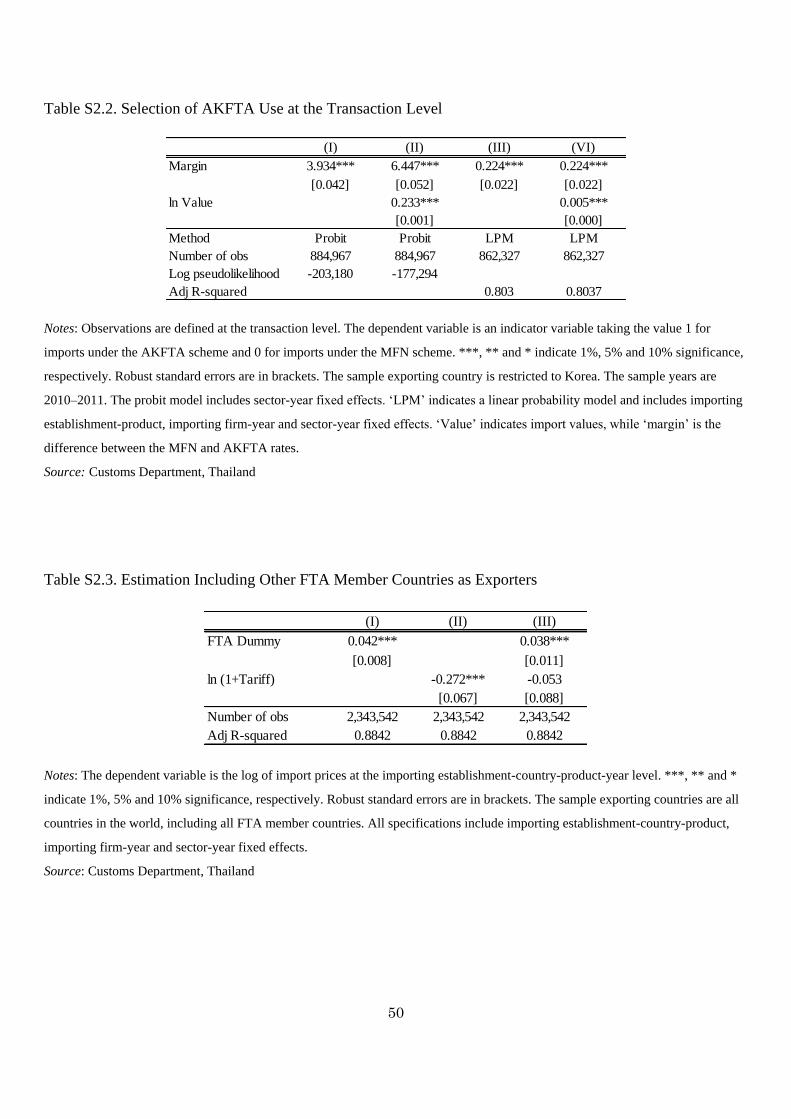
50

Table S2.2. Selection of AKFTA Use at the Transaction Level

(I) (II) (III) (VI)

Margin 3.934*** 6.447*** 0.224*** 0.224***

[0.042] [0.052] [0.022] [0.022]

ln Value 0.233*** 0.005***

[0.001] [0.000]

Method Probit Probit LPM LPM

Number of obs 884,967 884,967 862,327 862,327

Log pseudolikelihood -203,180 -177,294


Notes: Observations are defined at the transaction level. The dependent variable is an indicator variable taking the value 1 for

imports under the AKFTA scheme and 0 for imports under the MFN scheme. ***, ** and * indicate 1%, 5% and 10% significance,

respectively. Robust standard errors are in brackets. The sample exporting country is restricted to Korea. The sample years are

2010–2011. The probit model includes sector-year fixed effects. ‘LPM’ indicates a linear probability model and includes importing

establishment-product, importing firm-year and sector-year fixed effects. ‘Value’ indicates import values, while ‘margin’ is the

difference between the MFN and AKFTA rates.


Table S2.3. Estimation Including Other FTA Member Countries as Exporters

(I) (II) (III)

FTA Dummy 0.042*** 0.038***

[0.008] [0.011]

ln (1+Tariff) -0.272*** -0.053

[0.067] [0.088]

Number of obs 2,343,542 2,343,542 2,343,542

Adj R-squared 0.8842 0.8842 0.8842

Notes: The dependent variable is the log of import prices at the importing establishment-country-product-year level. ***, ** and *

indicate 1%, 5% and 10% significance, respectively. Robust standard errors are in brackets. The sample exporting countries are all

countries in the world, including all FTA member countries. All specifications include importing establishment-country-product,

importing firm-year and sector-year fixed effects.


51

Table S2.4. Estimation at the Transaction Level

(I) (II) (III) (IV)

FTA Dummy 0.028*** -0.079*** -0.282***

[0.010] [0.015] [0.016]

ln (1+Tariff) -0.553*** -1.083*** -1.056***

[0.098] [0.157] [0.137]

ln Value 0.370***

[0.000]

Number of obs 16,010,533 16,010,533 16,010,533 16,010,533

Adj R-squared 0.7451 0.7451 0.7451 0.7958

Notes: The dependent variable is the log of import prices at the transaction-level. ***, ** and * indicate 1%, 5% and 10%

significance, respectively. Robust standard errors are in brackets. All specifications include importing establishment-country-

product, importing firm-year and sector-year fixed effects.


52

Table S2.5. Decomposition of Rules of Origin Effects

(I) (II) (III)

FTA Dummy 0.111 0.136 0.442

[0.288] [0.287] [0.585]

FTA Dummy * CC/RVC -0.291

[0.276]

FTA Dummy * CH/RVC -0.174 -0.722

[0.266] [0.601]

FTA Dummy * CS/RVC 0.161 -0.612

[0.373] [0.611]

FTA Dummy * CH&RVC 0.215

[0.507]

FTA Dummy * RVC -1.050** -1.073** -1.764*

[0.463] [0.463] [0.911]

FTA Dummy * CTC/RVC -0.199

[0.264]

FTA Dummy * CTC&RVC 0.198

[0.507]

ln (1+Tariff) -1.299** -1.209*

[0.644] [0.642]

Base RoO WO WO WO

Products All All Ineligible

Number of obs 1,071,985 1,071,985 315,636

Adj R-squared 0.8719 0.8719 0.8763


indicate 1%, 5% and 10% significance, respectively. Robust standard errors are in brackets. All specifications include importing

establishment-country-product, importing firm-year and sector-year fixed effects. In this table, we interrelate the RTA dummy with

dummy variables indicating various RoO. ‘Ineligible’ in the products category indicates that the estimation sample products are

restricted to those in which the AKFTA rates are the same as the MFN rates.


53

Table S2.6. Tariff Effect and Demand Elasticity

BGW KNO

FTA Dummy -0.077 -0.064

[0.060] [0.065]

ln (1+Tariff) -1.551** -1.458*

[0.727] [0.751]

ln (1+Tariff) * Demand elasticity 0.049 -0.102***

[0.115] [0.038]

Number of obs 1,062,859 985,482



indicate 1%, 5% and 10% significance, respectively. Robust standard errors are in brackets. All specifications include importing

establishment-country-product, importing firm-year and sector-country-year fixed effects. In column ‘BGW’, we use the demand

elasticity obtained from the study by Broda, Greenfield and Weinstein (2006); whilst that from the study by Kee et al. (2008) is

used in column ‘KNO’. AKFTA is ASEAN-Korea free trade agreement. MFN refers to most-favored-nation. CH, RVC, CS, and

CTC are respectively change-in-heading, regional value content, change-in-subheading, and change-in-tariff classification.


54

Table S2.7. Other Estimations

(I) (II) (III)

FTA Dummy 1.687* -0.102 -0.089

[0.993] [0.072] [0.060]

FTA Dummy * ln Total Imports -0.598*

[0.338]

FTA Dummy * Preference Share 0.100

[0.128]

FTA Dummy * THB Invoice 0.376*

[0.212]

ln (1+Tariff) -1.327** -1.286** -1.510**

[0.598] [0.608] [0.604]

Number of obs 1,071,985 1,071,985 1,075,739

Adj R-squared 0.8719 0.8719 0.8721


indicate 1%, 5% and 10% significance, respectively. Robust standard errors are in brackets. The specifications in columns (I) and

(II) include importing establishment-country-product, importing firm-year and sector-year fixed effects. Column (III) includes

importing establishment-country-product-THB invoice, importing firm-year and sector-country-year fixed effects. ‘Total imports’

are the importing firms’ total imports of all products from the rest of the world. ‘Preference share’ indicates the share of imports

under all FTA schemes in total imports for each tariff-line product. ‘THB invoice’ is a variable taking the value 1 if the invoicing

currency is the Thai baht and 0 otherwise.


55

Appendix S3. Problems When Japanese Affiliates in Korea Export under FTA Schemes

Number %

No problems 9 29

Long time for obtaining CoOs 5 16

Shortage of staffs 4 13

Cumbersome RoOs across FTAs 3 10

No existence of FTAs 3 10

Unable to comply with RoOs 2 6

Cumbersome works for obtaining CoOs 2 6

Incooperative suppliers 2 6

Expensive CoO fee 1 3

Total 31

Notes: Multiple answers are allowed. The number of responding affiliates is 22.

Source: Survey of Japanese-Affiliated Firms in Asia and Oceania in 2011 (Japan External Trade Organization).

56

References

Asprilla, A., N. Berman, O. Cadot, and M. Jaud (2015), ‘Pricing-to-Market, Trade Policy, and Market

Power’, Working Paper N IHEIDWP04-2015, Geneva, Switzerland: The Graduate Institute of

International and Development Studies.

Broda, C., J. Greenfield, and D.Weinstein. 2006. From Groundnuts to Globalization: A Structural Estimate of

Trade and Growth. NBER Working Paper No. 12512, National Bureau of Economic Research,

Cambridge, MA.

Cadot, O. and J. de Melo (2007), ‘Why OECD Countries Should Reform Rules of Origin’, World Bank

Research Observer, 23(1), pp. 77–105.

Devereux, M., B. Tomlin, and W. Dong (2015), ‘Exchange Rate Pass-through, Currency of Invoicing and

Market Share’, NBER Working Paper No. 21413, Cambridge, MA: NBER.

Francois, J., B. Hoekman, and M. Manchin (2006), ‘Preference Erosion and Multilateral Trade

Liberalization’, World Bank Economic Review, 20(2), pp. 197–216.

Hansen, B. (2000), ‘Sample Splitting and Threshold Estimation’, Econometrica, 68(3), pp. 575–604.

Hayakawa, K. (2011), ‘Measuring Fixed Costs for Firms’ Use of a Free Trade Agreement: Threshold

Regression Approach’, Economics Letters, 113(3), pp. 301–303.

Kee, H. L., L. Nicita, and M. Olarreaga. 2008. “Import Demand Elasticities and Trade Distortions.” Review

of Economics and Statistics 90 (4): 666–82.

Maddala, G.S. (1983), Limited-dependent and Qualitative Variables in Econometrics, Cambridge, United

Kingdom: Cambridge University Press.

impact of free trade agreement use on import prices

Documents