training in household air pollution and...

Training in Household Air Pollution and MonitoringParo, Bhutan • 21 - 25 March 2016

Area MeasurementsEstimation, Measurement, and Analysis

COOKSTOVE EXPOSURE MONITORING PYRAMID

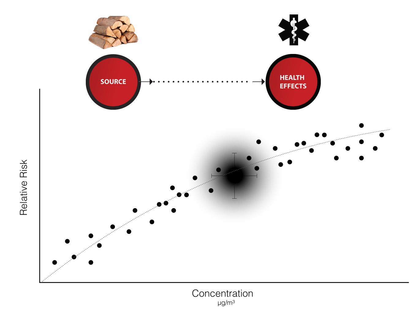
HEALTH EFFECT

National and Regional Fuel Use

Stove Usage

Emissions Sampling

Emissions Sampling + HH Characteristics

Micro-environmental Pollutant Concentrations

Micro-environmental + Time Activity

Personal Exposure

Personal Exposure + Time Activity

Biomarkers of Exposure

Biomarkers of Effect

COOKSTOVE EXPOSURE MONITORING PYRAMID

Stove Usage

Micro-environmental Pollutant Concentrations

Concentration µg/m3

Rela

tive

Risk

WOODSMOKE HEALTH EFFECTS: A REVIEW 69

TABLE 1Major health-damaging pollutants from biomass combustion

Compound Examplesa Source Notes Mode of toxicity

Inorganicgases

Carbon monoxide(CO)

Incompletecombustion

Transported over distances Asphyxiant

Ozone (O3) Secondary reactionproduct of nitrogendioxide andhydrocarbons

Only present downwind of fire,transported over long distances

Irritant

Nitrogen dioxide(NO2)

High-temperatureoxidation ofnitrogen in air, somecontribution fromfuel nitrogen

Reactive Irritant

Hydrocarbons Many hundreds Incompletecombustion

Some transport—also react to formorganic aerosols. Species vary withbiomass and combustion conditions

Unsaturated: 40+,e.g.,1,3-butadiene

Irritant, carcinogenic,mutagenic

Saturated: 25+,e.g., n-hexane

Irritant, neurotoxicity

Polycyclic aromatic(PAHs): 20+,e.g., benzo[a]pyrene

Mutagenic,carcinogenic

Monoaromatics:28+, e.g.,benzene, styrene

Carcinogenic,mutagenic

Oxygenatatedorganics

Hundreds Incompletecombustion

Some transport—also react to formorganic aerosols. Species vary withbiomass and combustion conditions

Aldehydes: 20+,e.g., acrolein,formaldehyde

Irritant, carcinogenic,mutagenic

Organic alcoholsand acids: 25+,e.g., methanolacetic acid

Irritant, teratogenic

Phenols: 33+, e.g.,catechol, cresol(methylphenols)

Irritant, carcinogenic,mutagenic,teratogenic

Quinones:hydroquinone,fluorenone,anthraquinone

Irritant, allergenic,redox active,oxidative stress andinflammation,possibly carcinogenic

Chlorinatedorganics

Methylene chloride,methyl chloride,dioxin

Requires chlorine inthe biomass

Central nervous systemdepressant (methylenechloride), possiblecarcinogens

(Continued on next page)

Inha

latio

n To

xico

logy

Dow

nloa

ded

from

info

rmah

ealth

care

.com

by

Prev

entio

n R

esea

rch

Cen

ter o

n 06

/21/

11Fo

r per

sona

l use

onl

y.

Products of Incomplete Combustion (PICs)What Could be measured in homes?

• Small particles, CO, NOX

• Hydrocarbons• 25+ saturated hydrocarbons such as n-hexane• 40+ unsaturated hydrocarbons such as 1,3 butadiene• 28+ mono-aromatics such as benzene & styrene• 20+ polycyclic aromatics such as benzo(a)pyrene

• Oxygenated organics• 20+ aldehydes including formaldehyde & acrolein • 25+ alcohols and acids such as methanol • 33+ phenols such as catechol & cresol

• Many quinones such as hydroquinone

• Semi-quinone-type and other radicals

• Chlorinated organics such as methylene chloride and dioxin“Toxic Waste Factory”

What can we measure in households?

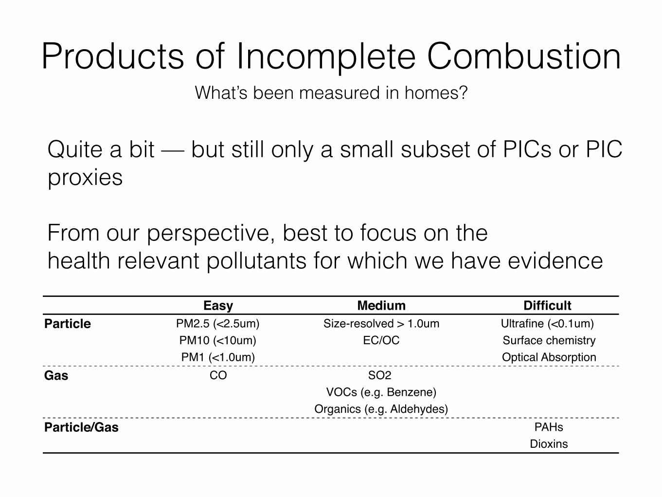
Products of Incomplete CombustionWhat’s been measured in homes?

Quite a bit — but still only a small subset of PICs or PIC proxies

From our perspective, best to focus on the health relevant pollutants for which we have evidence

Easy Medium Difficult Particle PM2.5 (<2.5um) Size-resolved > 1.0um Ultrafine (<0.1um)

PM10 (<10um) EC/OC Surface chemistryPM1 (<1.0um) Optical Absorption

Gas CO SO2 VOCs (e.g. Benzene)

Organics (e.g. Aldehydes)Particle/Gas PAHs

Dioxins

Monitoring KAP

ESTIMATE +PREDICT

SELECTDEVICES ANALYZEPERFORM

MEASUREMENTS

SAMPLING SCHEMEQA/QC PROCEDURES

SAMPLING SETUPDATA CLEANING

SAMPLE PROCESSING

Estimate

Predicting KAPApproximate before deciding on sampling schedule

(1) Literature Review

(2) Indoor models, using published emission rates, emission factors, and household characteristics

- Emissions are often measured in the lab - Estimate household characteristics

Why? - Measurement device selection - Sampling Duration - Hypothesis testing

Literature Review Examplehttp://www.who.int/indoorair/health_impacts/databases_iap/en/

! 40!

with location of 5, mean 50, and standard deviation of 85. A separate analysis for improved stoves was not used due to the limited number of scenarios. Modeling the distribution of CO concentrations from actual household data incorporates some of the influences of household factors on pollutant concentration, such as ventilation rate and room volume, that vary between locations.

Table 3.1. Descriptive statistics from 19 studies measuring average CO concentrations during meal preparation. All concentrations units are in ppm CO. Scenarios Studies Mean Min Max (ppm) (ppm) (ppm) Aggregated 35 (100%) 21 38 (48) 2 189 “Improved” 12 (34%) 7 21 (35) 2 130 “Traditional” 23 (66%) 14 47 (52) 6 189 P-value* 0.127 Values in parentheses represent one standard deviation *Student's ttest

3.2.3 Estimating Body Burden

COHb concentrations were estimated using the Peterson and Stewart regression model applied previously in chapter two, and based on non-smoking adults at a resting breathing rate [10] (Equation 2.1).

197%

63.0858.0 tCOCOHb �

Using Equation 3.1, we do not attempt to distinguish a difference in burden between children and adults due to limitations and assumptions inherently built into the model. Results from Chapter two would suggest, however, that the environmental model would underestimate burden in children more substantially than adults, likely due to their smaller body size and elevated breathing rates.

3.3 Simulation Results

3.3.1 Estimated COHb results

A Monte Carlo simulation for estimating %COHb based on environmental concentrations was performed using Crystal Ball (Oracle, Redwood Shores, CA, USA) under the parameters described previously. Estimated COHb concentrations from 50,000 trials using all stove types followed a lognormal distribution with mean and median of 3% (SD = 4%) and 2% COHb, respectively (Figure 2.1).

Equation 3.1

Lam, 2010

! 40!

with location of 5, mean 50, and standard deviation of 85. A separate analysis for improved stoves was not used due to the limited number of scenarios. Modeling the distribution of CO concentrations from actual household data incorporates some of the influences of household factors on pollutant concentration, such as ventilation rate and room volume, that vary between locations.

Table 3.1. Descriptive statistics from 19 studies measuring average CO concentrations during meal preparation. All concentrations units are in ppm CO. Scenarios Studies Mean Min Max (ppm) (ppm) (ppm) Aggregated 35 (100%) 21 38 (48) 2 189 “Improved” 12 (34%) 7 21 (35) 2 130 “Traditional” 23 (66%) 14 47 (52) 6 189 P-value* 0.127 Values in parentheses represent one standard deviation *Student's ttest

3.2.3 Estimating Body Burden

COHb concentrations were estimated using the Peterson and Stewart regression model applied previously in chapter two, and based on non-smoking adults at a resting breathing rate [10] (Equation 2.1).

197%

63.0858.0 tCOCOHb �

Using Equation 3.1, we do not attempt to distinguish a difference in burden between children and adults due to limitations and assumptions inherently built into the model. Results from Chapter two would suggest, however, that the environmental model would underestimate burden in children more substantially than adults, likely due to their smaller body size and elevated breathing rates.

3.3 Simulation Results

3.3.1 Estimated COHb results

A Monte Carlo simulation for estimating %COHb based on environmental concentrations was performed using Crystal Ball (Oracle, Redwood Shores, CA, USA) under the parameters described previously. Estimated COHb concentrations from 50,000 trials using all stove types followed a lognormal distribution with mean and median of 3% (SD = 4%) and 2% COHb, respectively (Figure 2.1).

Equation 3.1

Estimating KAP Concentrationsthe single compartment box model

Gα

VSingle box-model is basic, but reasonable, first approximation in many situations

Using information on pollutant emission factors/rates (G), room volume, and pollutant loss mechanisms such as air exchange rate or wall loss (α), we can approximate the indoor air pollutant concentration (Ct) at a point in time (t).

Estimating KAP Concentrationsthe single compartment box model

G

α

V

used tools in air pollution and climate studies (Bond et al., 2011;Hellweg et al., 2009; Nicas, 2008), yet have not been relied uponas tools for informing on the impact of improved stove projects.Modeling approaches pose several potential benefits, including: 1)estimating potential impacts on indoor air pollution concentrationsbefore conducting expensive and time consuming field studies; 2)evaluating relative importance and impacts of critical stoveperformance parameters and environmental variables; and 3)providing a means to set stove performance benchmarks or stan-dards which are explicitly linked to air quality guidelines.

There is growing interest in setting standards for stove perfor-mance as part of international efforts to promote clean cookstoves.Currently there are globally accepted performance standards forbiomass cookstoves, although the Shell Foundation/AprovechoBenchmarks have been used in laboratory testing for guidance andevaluation of stove design (MacCarty et al., 2010). These bench-marks, however, are not linked to air quality guidelines and arenormalized to a standardized water boiling test, which has beenshown to be a poor predictor of emissions from normal stove use inhomes (Johnson et al., 2008, 2009; Roden et al., 2009).

This paper presents a first approach toward addressing theseneeds with a simple Monte Carlo single-box model, which predictsindoor concentrations given a stove’s emission performance andusage, as well as kitchen characteristics. Here we illustrate theutility of the model by presenting simulated distributions of IAPconcentrations in kitchens based on a series of stove/fuel scenarios,comparing them with the World Health Organization (WHO) AirQuality Guidelines (AQGs) for PM2.5 and CO. Finally, the model isused to predict the stove performance characteristics that would berequired for a given percentage of homes to meet the WHO AQGs.

2. Methods

2.1. Monte Carlo single-box model

The single-box model employed here predicts room concentra-tions based on stove emissions and kitchen characteristics. Indoorair pollutant concentrations were modeled assuming a well mixedroom with single constant emission source. The model assumesinstantaneousmixing with zero backflow to the room, that removalof the pollutant from the air is dominated by ventilation, andcompeting loss mechanisms are negligible (e.g. surface reactions,particle settling). The model is described mathematically as:

Ct ¼ GfaV

!1" e"at

"þ Co

!e"at

"; (1)

where, Ct ¼ Concentration of pollutant at time t (mg m"3);G ¼ emission rate (mg min"1); a ¼ first order loss rate (nominal airexchange rate) (min"1); V ¼ kitchen volume (m3); t ¼ time (min);C0 ¼ concentration from preceding time unit (mgm"3); f¼ fractionof emissions that enters the kitchen environment.

The emission rate and cooking duration are functions of thepower, thermal efficiency, and emission factors for a given fuel/stove combination, as well as the amount of required energy-delivered for cooking. Emission rate G was calculated as:

G ¼EFED

P; (2)

where EF is the fuel based emission factor (mg pollutant kg fuel"1),ED is the energy density of the fuel (MJ kg"1)1, and P is the stovepower (MJ min"1). Emission rates were constant during each

cooking event for each respective model iteration. Daily cookingenergy requiredwas split into three equal events, with the duration(TC) of each determined as:

TC ¼ EDC=3PðhÞ ; (3)

where EDC is total daily cooking energy required (MJ) and h isstove’s thermal efficiency (%).

A Monte Carlo approach was used to incorporate the variabilityin model parameters, resulting in a predicted distribution of PM2.5and CO concentrations. 5000 simulations of a day of cooking wererun, with the inputs randomly selected from their respectiveprobability distribution.

2.2. Model inputs

For the purposes of illustrating the model, we present resultsbased on inputs selected to represent scenarios specific to theIndian context, although the model can be applied to any regionwhere sufficient data is available. Indiawas selected as the availabledata for inputs was relatively comprehensive, and it representsa country with a large number of homes using solid fuel stoves.Four different scenarios were run to illustrate the utility of themodel: 1) wood-burning traditional chulha with inputs based oncontrolled cooking tests2 conducted in Indian homes by regularstove users; 2) wood-burning Envirofit G3300 rocket stove withinputs based on controlled cooking tests conducted in Indianhomes by regular stove users; 3) the same Envirofit G3300 stovewith inputs based on water boiling tests3 conducted in the labo-ratory; and 4) an LPG stove with inputs based onwater boiling testsconducted in the laboratory. Table 1 provides a summary of themodel parameters and their basis for use in the model.

Air exchange rate distributions were based on three studiesconducted in India, which were estimated from the decay rate ofcarbon monoxide after the conclusion of a cooking event(McCracken and Smith, 1998). Distributions of kitchen volumeswere also estimated based on measurements in Indian homes.Daily cooking energy for India was obtained from an analysis byHabib et al. (2004), who combined national survey data for foodconsumption with the specific energy required for cookingcommon foods. Emission factors, thermal efficiency, and stovepower were drawn from four sources: Inputs for in-home use oftraditional chulhas and the G3300 were from a study by BerkeleyAir Monitoring Group and Sri Ramachandra University in TamilNadu, which was conducted using a series of controlled cookingtests in 10 rural homes. The lab-based inputs for the G3300 werefrom water boiling tests conducted at the Engines and EnergyConversion Lab at Colorado State University. The inputs for LPGemission factors, thermal efficiency, and power were from Smithet al. (2000), with an additional PM emission factor for LPG fromHabib et al. (2008) included in the mean.

All distributions were assumed to be lognormal, which iscommon for environmental data. Distributions were truncated atlimits deemed highly improbable for the given parameter, whilestill allowing relatively extreme, yet possible data points (e.g. verysmall or large kitchens). All truncated distributions contained over90% of the data of the entire distribution. The fraction of emissions

1 18 MJ kg"1 for dry wood and 46 MJ kg"1 for LPG (Smith et al., 2000).

2 The controlled cooking test is a stove performance test where a typical, localmeal is prepared by local cooks on multiple stoves in order to compare stoveperformance metrics to complete a typical cooking task.

3 The water boiling test is a standardized laboratory test where water is broughtto a boil and then simmered for 45 min, from which various stove performancemetrics can be derived.

M. Johnson et al. / Atmospheric Environment xxx (2011) 1e72

Please cite this article in press as: Johnson, M., et al., Modeling indoor air pollution from cookstove emissions in developing countries usinga Monte Carlo single-box model, Atmospheric Environment (2011), doi:10.1016/j.atmosenv.2011.03.044

Emission Rate (mass/time)Loss Rate, Ventilation ( 1/hr)Volume (cubic meters)Background concentration (mass/vol)Fraction emitted to environment (0-1)

GAlpha

VCo

f

SKIP

Estimating KAP ConcentrationsAt steady-state, assuming instantaneous mixing

Emission Rate (mass/time)Loss Rate, Ventilation ( 1/hr)Volume (cubic meters)Fraction emitted to environment (0-1)

GAlpha

Vf

used tools in air pollution and climate studies (Bond et al., 2011;Hellweg et al., 2009; Nicas, 2008), yet have not been relied uponas tools for informing on the impact of improved stove projects.Modeling approaches pose several potential benefits, including: 1)estimating potential impacts on indoor air pollution concentrationsbefore conducting expensive and time consuming field studies; 2)evaluating relative importance and impacts of critical stoveperformance parameters and environmental variables; and 3)providing a means to set stove performance benchmarks or stan-dards which are explicitly linked to air quality guidelines.

There is growing interest in setting standards for stove perfor-mance as part of international efforts to promote clean cookstoves.Currently there are globally accepted performance standards forbiomass cookstoves, although the Shell Foundation/AprovechoBenchmarks have been used in laboratory testing for guidance andevaluation of stove design (MacCarty et al., 2010). These bench-marks, however, are not linked to air quality guidelines and arenormalized to a standardized water boiling test, which has beenshown to be a poor predictor of emissions from normal stove use inhomes (Johnson et al., 2008, 2009; Roden et al., 2009).

This paper presents a first approach toward addressing theseneeds with a simple Monte Carlo single-box model, which predictsindoor concentrations given a stove’s emission performance andusage, as well as kitchen characteristics. Here we illustrate theutility of the model by presenting simulated distributions of IAPconcentrations in kitchens based on a series of stove/fuel scenarios,comparing them with the World Health Organization (WHO) AirQuality Guidelines (AQGs) for PM2.5 and CO. Finally, the model isused to predict the stove performance characteristics that would berequired for a given percentage of homes to meet the WHO AQGs.

2. Methods

2.1. Monte Carlo single-box model

The single-box model employed here predicts room concentra-tions based on stove emissions and kitchen characteristics. Indoorair pollutant concentrations were modeled assuming a well mixedroom with single constant emission source. The model assumesinstantaneousmixing with zero backflow to the room, that removalof the pollutant from the air is dominated by ventilation, andcompeting loss mechanisms are negligible (e.g. surface reactions,particle settling). The model is described mathematically as:

Ct ¼ GfaV

!1" e"at

"þ Co

!e"at

"; (1)

where, Ct ¼ Concentration of pollutant at time t (mg m"3);G ¼ emission rate (mg min"1); a ¼ first order loss rate (nominal airexchange rate) (min"1); V ¼ kitchen volume (m3); t ¼ time (min);C0 ¼ concentration from preceding time unit (mgm"3); f¼ fractionof emissions that enters the kitchen environment.

The emission rate and cooking duration are functions of thepower, thermal efficiency, and emission factors for a given fuel/stove combination, as well as the amount of required energy-delivered for cooking. Emission rate G was calculated as:

G ¼EFED

P; (2)

where EF is the fuel based emission factor (mg pollutant kg fuel"1),ED is the energy density of the fuel (MJ kg"1)1, and P is the stovepower (MJ min"1). Emission rates were constant during each

cooking event for each respective model iteration. Daily cookingenergy requiredwas split into three equal events, with the duration(TC) of each determined as:

TC ¼ EDC=3PðhÞ ; (3)

where EDC is total daily cooking energy required (MJ) and h isstove’s thermal efficiency (%).

A Monte Carlo approach was used to incorporate the variabilityin model parameters, resulting in a predicted distribution of PM2.5and CO concentrations. 5000 simulations of a day of cooking wererun, with the inputs randomly selected from their respectiveprobability distribution.

2.2. Model inputs

For the purposes of illustrating the model, we present resultsbased on inputs selected to represent scenarios specific to theIndian context, although the model can be applied to any regionwhere sufficient data is available. Indiawas selected as the availabledata for inputs was relatively comprehensive, and it representsa country with a large number of homes using solid fuel stoves.Four different scenarios were run to illustrate the utility of themodel: 1) wood-burning traditional chulha with inputs based oncontrolled cooking tests2 conducted in Indian homes by regularstove users; 2) wood-burning Envirofit G3300 rocket stove withinputs based on controlled cooking tests conducted in Indianhomes by regular stove users; 3) the same Envirofit G3300 stovewith inputs based on water boiling tests3 conducted in the labo-ratory; and 4) an LPG stove with inputs based onwater boiling testsconducted in the laboratory. Table 1 provides a summary of themodel parameters and their basis for use in the model.

Air exchange rate distributions were based on three studiesconducted in India, which were estimated from the decay rate ofcarbon monoxide after the conclusion of a cooking event(McCracken and Smith, 1998). Distributions of kitchen volumeswere also estimated based on measurements in Indian homes.Daily cooking energy for India was obtained from an analysis byHabib et al. (2004), who combined national survey data for foodconsumption with the specific energy required for cookingcommon foods. Emission factors, thermal efficiency, and stovepower were drawn from four sources: Inputs for in-home use oftraditional chulhas and the G3300 were from a study by BerkeleyAir Monitoring Group and Sri Ramachandra University in TamilNadu, which was conducted using a series of controlled cookingtests in 10 rural homes. The lab-based inputs for the G3300 werefrom water boiling tests conducted at the Engines and EnergyConversion Lab at Colorado State University. The inputs for LPGemission factors, thermal efficiency, and power were from Smithet al. (2000), with an additional PM emission factor for LPG fromHabib et al. (2008) included in the mean.

All distributions were assumed to be lognormal, which iscommon for environmental data. Distributions were truncated atlimits deemed highly improbable for the given parameter, whilestill allowing relatively extreme, yet possible data points (e.g. verysmall or large kitchens). All truncated distributions contained over90% of the data of the entire distribution. The fraction of emissions

1 18 MJ kg"1 for dry wood and 46 MJ kg"1 for LPG (Smith et al., 2000).

2 The controlled cooking test is a stove performance test where a typical, localmeal is prepared by local cooks on multiple stoves in order to compare stoveperformance metrics to complete a typical cooking task.

3 The water boiling test is a standardized laboratory test where water is broughtto a boil and then simmered for 45 min, from which various stove performancemetrics can be derived.

M. Johnson et al. / Atmospheric Environment xxx (2011) 1e72

Please cite this article in press as: Johnson, M., et al., Modeling indoor air pollution from cookstove emissions in developing countries usinga Monte Carlo single-box model, Atmospheric Environment (2011), doi:10.1016/j.atmosenv.2011.03.044

ss

Information Emission Factor = 2.0 g pollutant / kg fuel (lab)Fuel Consumption Rate = 1.0 kg fuel/hr (lab, field)Kitchen Volume = 40 cubic-meters (estimated, field)Air Exchange rate per hour (ACH) = 8/hr (estimated, field) Fraction to Indoor Environment (f) = 1.0 (non-chimney)

Steady State Level Ctss = (2.0 g/kg*1.0 kg/hr) *1 / 8/hr * 40m3 Ctss = 0.0063 g/m3 = 6.3 mg/m3

24hr Average (Assume 6 hrs of cooking/day, background is zero )

C24hr TWA = (6/24)*6.3mg/m3 + (18/24)*0mg/m3 = 1.6mg/m3

CalculationsSKIP

Want more?

Select Devices

Sampling in households is complicated

Devices need to be quiet, as they are placed in common areas in households, like kitchens and bedrooms

The sampling environments are harsh, and equipment is exposed to high concentrations of pollutants. Devices must be robust, repairable, relatively inexpensive, and battery operated

Due to the difficulties of fieldwork, devices need to be lightweight, portable, and require minimal field staff intervention

Need to be able to access devices easily to make sure they are operating properly

DeviceCharacteristics

an overview

How the sample is obtained(active or passive)

+

The form of the data(integrated or real-time)

Human hair 50–70 μm in diameter

PM 2·5Eg, combustion particles, organic

compounds, metals <2·5 μm in diameter

PM 10Eg, dust, pollen, mould <10 μm in diameter

90 μm in diameterFine beach sand

Measuring Particulate MatterPM of primary concern from a health perspective

PM size is conventionally referred to by its aerodynamic diameter: the diameter of a sphere of water with the same aerodynamic properties as the particles in question

Adapted from Guarnieri et al 2014

PM Size ConventionsUpper respiratory tract

Nasopharynx

Ultr

afine

PM

(PM

<0·

1 μm

) Trachea

Bronchi/bronchioles

Alveoli

Oropharynx

Larynx

Lower respiratory tract

Fine

PM

(PM

2·5

μm

)

Coar

se P

M (P

M 2

·5–1

0 μm

)

Ultr

afine

PM

(PM

<0·

1 μm

)

Adapted from Guarnieri et al 2014

PM Size ConventionsUpper respiratory tract

Nasopharynx

Ultr

afine

PM

(PM

<0·

1 μm

) Trachea

Bronchi/bronchioles

Alveoli

Oropharynx

Larynx

Lower respiratory tract

Fine

PM

(PM

2·5

μm

)

Coar

se P

M (P

M 2

·5–1

0 μm

)

Ultr

afine

PM

(PM

<0·

1 μm

)

Guarnieri et al 2014

Particle sampling devices and inlet-ports limit the particle sizes that are collected or measured in accordance with these cutoffs and/or distribution shapes.

Filter-based or gravimetric samplingGold-standard for PM sampling - Active, integrated

Basic Theory:

1) Air sample is passed through a filter using a pump, capturing or impacting particles onto the filter media, at a specific flow rate

2) Particle mass (ug) is measured using a microbalance and sampled air volume is calculated using measured flow rates.

Many filter media exist depending type of analysis (e.g. Teflon, PVC, Quartz, glass fiber, various coating combinations)

Air fl

ow

Filter

BGI USA

BGI Triplex: PM 4PM 2.5PM 1

Aerodynamic Diameter (um)

3.5 lpm 1.5 lpm 1.05 lpm

Gold Standard method for measuring PM mass concentrations. Flow rates correspond to specific size cutoffs or

distributions (D50).

Manufactures should provide validation material the device (e.g.

penetration curves)

Cyclones and Impactors select for particle sizes or distributions using

particle dynamics in airstreams

Personal samplers often used as environmental samplers (size, flow

rates, battery life)

http://aerosol.ees.ufl.edu/

Filter-based or gravimetric samplingActive, integrated samplers

BGI Respirable / Thoracic cyclone

SKC Cascade Impactor

SKC Personal Exposure Monitor

http://aerosol.ees.ufl.edu/

Filter-based or gravimetric samplingActive, integrated samplers - Workflow

Casella Apex Pro

SKC Personal

Pump

0.5 - 6 lpm

1.5 lpm (PM2.5)

Filters and holders ($5-10 + labor), sampler ($350+), tubing (<$20), pump ($500+)

Flow calibration ($100s - 1000+)

Selecting Pumps - Battery life, flow rate requirements, and noise.

Flow compensation for consistent flow rate as filter loads and creates increasing resistance

Filter-based or gravimetric samplingWorkflow - Step by Step

PREPARATION SAMPLING CALCULATIONSPOSTWEIGHING

Equilibrate Pre-Weigh

Prepare Cassettes

Leak Check Cassette Pre/Post Flow rates Sample Duration

Field Blanks Transport

Equilibrate Post-Weigh

Adjust for blanks

Pre Mass (ug) Sample + Blanks

Sample Volume (m3) + Duration (hrs, days)

Post Mass (ug) Sample + Blanks

Mass Concentration

(ug/m3)

!!"# ! !!"#$ ! !"# ! !"#$%

!"#$%& !

Light Scattering Devices

UCB Particle Monitor

Smoke enters and exits through diffuser

Current source drives pulses to IR LED

Photodetector

Light scattered by smoke particles

The relationship between scattering and mass concentration is affected by the aerosol and environmental conditions.

To obtain accurate mass conc. light scattering devices must be calibrated or co-located using filters, using the aerosol of interest, under field conditions.

Light scattering is not a direct measure of mass concentration but can be related.

Active, direct-reading instrumentsMany on the market!

TSI SidePak (~$5000)

Thermo PDR w/ cyclone (~$4000)

Aprovecho IAP Meter (~$3000)

Devices vary by measurement range, size, cost, sensitivity, validation

Measure light scattering, not mass. Must be compared against filter-based measurements.

Aerosol mixtures pose adjustment challenges

Selection Considerations: Range of levels expected Duration of sampling (battery) Budget

TSI DustTrak (~$8500)

RTI MicroPEM (~$3000)

Passive, direct-reading instruments

Ideal for KAP field studies

Low-power consumption

High range

Robust, easy to clean and service

UCB-PATS used in dozens of studies around the world

~500 USD

Passive, direct-reading instruments

PATS+

Wide dynamic range10µg/m3 to 50mg/m3

Modern microelectronicsUSB, SD card

Long-battery life

Coming soon from Berkeley Air

We’ll use with them later today

All light-scattering, direct reading instruments must be calibrated against the aerosol of interest

Adjust the response on the monitor

Ex post facto apply a 'calibration factor'

or

Particle CalibrationsOnce in the lab, at least once in the field

Light scattering devices should be calibrated against filter-based samples or filter-calibrated instruments.

Ideally, tests in lab first with aerosol of interest, then in-field co-locations to account for differences in

aerosol mixtures.

Does not require complex chamber but is a critical step since intra-instrument variability combined with

response can be a major source of error!


2200–3000 m) from August 2002 to January 2005.5 One-eighth(n = 69) of the 530 households in RESPIRE, were intensivelymonitored for particulate matter and carbon monoxide.Reported here are the results of deploying two separate UCBsin each intensively monitored household with simultaneousgravimetric assessment of fine particulate matter (PM2.5) everythree months. Standard protocols were followed in placingequipment on the wall of the kitchen: 145 cm above the floor,100 cm from the edge of the combustion zone of the cookingstove and at least 150 cm away (horizontally) from openabledoors and windows. PM2.5 was measured over 48 h in thekitchen using the SKC 224-PCXR8 pump programmed tooperate every 1 min out of 5 using a BGI SCC1.062 Triplexcyclone with a flow rate of 1.5 l min!1. Initial 24 h supervision,and 48 h final flow rates were measured with a rotameter toensure proper functioning of equipment. The rotameter wascalibrated with a laboratory Gilibrator (Gilian Model, Sensi-dyne, Clearwater, FL, USA) every 3 months. 37 mm PTFETEFLO filters (SKC Inc., Eighty Four, PA, USA) with poresize of 1 micron were used as the particle collection media. Thefilters were pre-weighed and post-weighed with a 6-placeMettler Toledo MT-5 microbalance at the Harvard UniversitySchool of Public Health. The weighing room was controlledfor temperature (21.9 " 0.8 1C) and relative humidity (41.8 "1.7%); barometric pressures (101.4 " 1.1 kPa) were alsonoted. Static electricity was discharged before each weighingby passing each side of the filter near a polonium 210 alpha-radiation source for a few seconds. Lab blanks were weighedevery 10 filter weights to ensure the lab blank readings werewithin 5 mg of the standard reading during the entire weighingsession. Each sample filter was weighed at least 2 times untilthe mass difference between the repeated weighing was equalto or less than 5 mg. Field blanks were assessed concurrently(average change in weight of !0.001 " 0.005 mg, n = 48).Since this was negligible, no blank subtraction was performed.Laboratory and field sampling forms and UCB results weredouble entered and discrepancies resolved against data collec-

tion forms. Subsequently, to see if any error was found, filterweights were merged using SAS (Version 9.1) and 20% of preand post filter weights checked manually.

Results and discussion

Controlled co-location tests in Mexico

Fig. 2 shows the different concentration peaks generated toevaluate the UCB and DustTrak responses. Peak combustionevents were chosen rather than continuous exposure periodsbecause (1) they are indicative of the dynamic range ofconcentrations over a 24 h period in rural households thatrely on biomass in open fires for energy provision both interms of concentration and in terms of the dynamic changes inconcentration during cooking periods; and (2) they provide abetter evaluation of instrument performance as decreases insensitivity over the study period are easier to identify. Amixing fan was present to minimize spatial concentrationdifferences that may impact the estimation of instrumentperformance.The correlation matrix in Table 1 shows the Pearson r2

exceeding 0.99 for each pair of instruments in one co-locationtest, and Table 2 shows the summarized results for the 4different co-location tests. As might be expected for differentmonitors, the slope of the response was slightly different foreach UCB, highlighting the need for individual instrumentcalibrations, similar to many other air pollution monitors.Although slightly lower, as seen in Table 2, correlations werehighly and consistently correlated with the DustTrak, withaverage Pearson r2 values exceeding 0.986 for each co-location.Fig. 3 shows a comparison of DustTrak and unadjusted

UCB response for each peak exposure event in the 4 testsshowing that the UCB sensitivity remained linear through awide range of peak concentrations that would be found inbiomass-burning kitchens (slope = 0.06; see also Table 2).

Fig. 2 Responses of 19 UCBs and DustTrak during chamber tests.

This journal is #c The Royal Society of Chemistry 2007 J. Environ. Monit., 2007, 9, 1099–1106 | 1101

Intra-instrument variability


Adjustment for inter-instrument differences in sensitivity can,therefore, be applied across the range of these concentrationswithout significant bias introduced. Although the UCBshowed consistently good relationships with DustTrak sensi-tivity on a minute by minute basis (Table 1), as peak particu-late masses increase, the UCB is more sensitive than theDustTrak for the size distributions generated in these tests.The slightly poorer correlation between the UCB : DustTrakand the UCB : UCB in the tests are due to these sensitivitydifferences between the UCB and the DustTrak response. Thisis not surprising between nephelometers using different wave-lengths.Fig. 4 shows the relationship between the UCB mV response

and gravimetric filters collected during the different chambertests. For clarity, only 3 UCBs are displayed in the graph, butthe remaining 16 showed similar response (Table 2). The UCBresponse correlated well with gravimetric filter mass, althougheach UCB showed a slightly different sensitivity compared togravimetric mass, as would be expected between differentmonitors. UCB response also agreed well with DustTrakresponse shown in the graph, although, as has been reportedby others,6–9 the unadjusted DustTrak without calibrationwith the aerosol of interest overpredicted the mass of thiscombustion aerosol by a factor of 3.1 compared to TeflonPM2.5 mass estimates over the course of the 4 experiments. Nodecay in UCB particulate mass sensitivity in relation to PM2.5

gravimetric estimates was observed between the 4 co-locationtests, even though at the time, the UCBs were being used 5days a week over a 6 week period in an intensive monitoringexercise of kitchens using open fires in Mexico. Therefore, theresults demonstrated that the UCB, with an appropriatecleaning protocol as described in the methods, may be usedto provide consistent estimates of PM2.5 mass over the courseof most field monitoring exercises. Clearly, to ensure properUCB performance during the entire duration of very long fieldprojects that sample in high particulate environments, a con-

sistent quality assurance monitoring strategy such as thecontrolled co-location tests presented here should be used.The relationship between the UCB mV response and both

PVC and Teflon PM2.5 mass estimates in co-location tests arepresented in Table 3. The coefficient of variation of theunadjusted UCB mass response in relation to gravimetricestimates was 15%. Therefore, if such controlled co-locationtests are not performed between UCBs in field studies, a biasof 15% can be expected between mass estimates of differentUCBs because of innate differences in sensitivity among thecommercial smoke detector chambers. As a result, to check fordefective components, controlled comparisons such as theseare performed routinely after manufacture but prior to de-ployment in the field. Although identical pumps and cycloneswere used, PM2.5 mass estimates were higher for PVC filterscompared to Teflon filters in these co-location tests. Ascorrelations between filter types were high, a systematic dif-ference in particle capture efficiency may exist between them.To standardize any bias in gravimetric estimates, therefore,Teflon filters should probably be used when making thesecomparisons.Although substantially improving accuracy compared to no

calibration with combustion aerosols, controlled co-locationtests such as these do not fully simulate actual field conditionsbecause of the potential for different size distributions ofcombustion aerosols in the households compared to the con-trolled co-location tests even when the same fuel is used. Inreal biomass-burning households, for example, there is amixture of flaming and smoldering combustion, which gener-ate aerosols with quite different size distributions.10,11 In theco-location tests, we consistently used smoldering pieces offuel for several reasons: (1) it is extremely difficult to effectivelycontrol the balance of flaming and smoldering phases duringcombustion events in a test. Small differences in this balancebetween different phases of combustion would significantlyimpact the particle size distributions present at each burn in

Table 2 Summary correlations between 19 UCBs and a DustTrak for 4 chamber tests

Pearson r2 Co-location 1 Co-location 2 Co-location 3 Co-location 4

Average inter UCB correlation (N = 19) 0.993 ! 0.003 0.998 ! 0.002 0.994 ! 0.009 0.998 ! 0.001Correlation between 19 UCBs and DustTrak 0.986 ! 0.002 0.993 ! 0.003 0.989 ! 0.010 0.998 ! 0.001

Fig. 3 Correlation of mean UCB peak response with DustTrak

during 4 chamber tests (N = 19).

Fig. 4 Correlation of UCB response with PM2.5 Teflon gravimetric

filters collected during 4 tests.

This journal is "c The Royal Society of Chemistry 2007 J. Environ. Monit., 2007, 9, 1099–1106 | 1103


Room ExhaustAir Flow

ValveMixing Fan

Sampling Probe

Valve

HEPA

Why calibrate in the field?

Field-based conversion factors calculated for Open Fire and Patsari stoves differed significantly

Using the Open Fire conversion factor for the Patsari would have resulted in an underestimation of the PM concentration by ~57%.

Fuel and stove type can influence light scattering response

In-field co-location with filter-based samples on subsample must be used for most accurate data.

Mean 24-h PM2.5 concentrations in homes with improved Pat-sari stoves were 60% (Student’s t-test, p < 0.01) lower than homeswith open fires (0.101 mg m!3and 0.257 mg m!3, respectively).Similarly, mean personal exposures were 50% (Student’s t-testp < 0.01) lower for the primary cooks in homes with improvedPatsari stoves compared to primary cooks in homes with open fires(0.78 mg m!3 and 0.156 mg m!3, respectively). Fig. 4 showsa comparison of reductions in kitchen concentrations in Tanacocompared to reductions in indoor PM2.5 concentrations in a nearbycommunity Comachuén (Armendáriz Arnez et al., 2008). Althoughthe percentage reductions in the two communities differ (50%compared to 67% respectively), the percentage reductions are moreinfluenced by the initial concentrations in the home as theimproved stove reduces concentrations consistently across homes.

Table 2 shows the correlation of co-located semi-continuousUCBparticle monitors with the size fractions measured with the Sioutascascade impactor in kitchens with open fire and improved Patsaristoves. The light scattering UCB particle monitor correlated bestwith the size fraction 0.25e0.5 mm for both homes with open fires(r2 ¼ 0.85) and homes with improved Patsari stoves (r2 ¼ 0.86).Subsequently the light scattering monitor correlated best with thesmallest size fraction for the open fire, as this size fractioncontributed the greatest to mass concentrations, but the larger sizefractions for the Patsari improved stove, as the larger size fractions

have a greater relative contribution to mass concentrationscompared to the open fire and light scattering sensor in the UCB ismore sensitive to the larger size particles (Edwards et al., 2006;Litton et al., 2004).

4. Discussion

Mass median diameter (MMD) of indoor PM2.5 particulatematter increased by 29% with the Patsari improved stove comparedto the open fire (from 0.59 mm to 0.42 mm, respectively). Thesefindings are comparable to other studies; Venkataraman and Rao(2001) reported unimodal distributions with MMDs of0.5e0.8 mm across 4 stove types for PM emissions from biofuelcombustion, and Li et al. (2007) reported a bimodal distributionwith a prominent mode at 0.12e0.32 mm and a smaller mode at0.76 mm during the whole burning cycle of woody fuels. AlthoughTanaco has unpaved streets with considerable fine dust resulting inhigh concentrations of resuspended dust that had a characteristi-cally different color in the largest size cut of the Sioutas cascadeimpactor (Fig. 2), over 80% of particle mass concentrations in theseindoor environments were submicron consistent with otherstudies. For example, inside a simulated village house Smith (1987)found that an open cook burning stove released 85% of total PMmass emissions as sub-micrometer particles. Reid et al. (2005)reported that approximately 80e90% of the volume of biomassburning particles is in the accumulation mode (dp< 1 mm) and Parkand Lee (2003) found that for all biofuel combustion cases, 90% ofthe mass of PM was between 0.03 and 2.39 mm.

0.00

0.05

0.10

0.15

0.20

0.25

0.30

0.35

Open Fire Patsari

MP5.2

mg

m(3-)

1.0-2.50.5-1.00.25-0.5<0.25

11%

48%

20%12%20%67%

15%

7%

Size bin (µm)n=11

n=10

0.00

0.05

0.10

0.15

0.20

0.25

0.30

0.35

Open Fire Patsari

mg

m(PS

T3-)

>2.5

1.0-2.5

0.5-1.0

0.25-0.5

<0.25

19%

34%

14%9%

14%

29%55%

12%

5%9%

Size bin (µm)n=11

n=10

Fig. 3. Relative contributions of size fractions to TSP and PM2.5 mass concentrations in homes with open fires and homes with improved Patsari stoves.

y = 0.84x - 0.068r² = 0.89

-0.2

0

0.2

0.4

0.6

0.8

1

1.2

1.4

0 0.5 1 1.5 2

Open fire PM2.5 (mg/m3)

MPirastaP-erif

nepO

5.2m/g

m(3 )

ComachuenTanaco (mean)

Fig. 4. Cross sectional PM2.5 mass concentrations in indoor air of homes with openfires and improved Patsari stoves in Tanaco compared to before and after measure-ments with the same stove types in a nearby community Comachuén.

Table 2Correlation betweenUCB particlemonitors and size fractions of particulatematter inindoor air for homes with open fires and improved Patsari stoves.

PM sizefraction (mm)

Open Fire Patsari Differencein b1b1 (mg m!3

per mv)r2 b1 (mg m!3

per mv)r2

<0.25 0.028 0.65 0.025 0.56 L11%0.25-0.5 0.0037 0.85 0.014 0.86 280%0.5e1.0 0.0014 0.55 0.0059 0.49 320%1.0e2.5 0.0014 0.34 0.0093 0.65 560%>2.5 0.0021 0.19 0.012 0.43 470%

TSP 0.037 0.69 0.066 0.63 78%PM2.5 0.035 0.70 0.055 0.67 57%

Notes: b1 represents the slope in the linear regression equation, y

ˇ

¼ b0 þ b1x, wherey

ˇ

is the predicted PM size fraction, b0 is the intercept, and x is the UCB-PM millivoltresponse. All regressions were significant at p < 0.05.

C. Armendáriz-Arnez et al. / Atmospheric Environment 44 (2010) 2881e28862884

Mean 24-h PM2.5 concentrations in homes with improved Pat-sari stoves were 60% (Student’s t-test, p < 0.01) lower than homeswith open fires (0.101 mg m!3and 0.257 mg m!3, respectively).Similarly, mean personal exposures were 50% (Student’s t-testp < 0.01) lower for the primary cooks in homes with improvedPatsari stoves compared to primary cooks in homes with open fires(0.78 mg m!3 and 0.156 mg m!3, respectively). Fig. 4 showsa comparison of reductions in kitchen concentrations in Tanacocompared to reductions in indoor PM2.5 concentrations in a nearbycommunity Comachuén (Armendáriz Arnez et al., 2008). Althoughthe percentage reductions in the two communities differ (50%compared to 67% respectively), the percentage reductions are moreinfluenced by the initial concentrations in the home as theimproved stove reduces concentrations consistently across homes.

Table 2 shows the correlation of co-located semi-continuousUCBparticle monitors with the size fractions measured with the Sioutascascade impactor in kitchens with open fire and improved Patsaristoves. The light scattering UCB particle monitor correlated bestwith the size fraction 0.25e0.5 mm for both homes with open fires(r2 ¼ 0.85) and homes with improved Patsari stoves (r2 ¼ 0.86).Subsequently the light scattering monitor correlated best with thesmallest size fraction for the open fire, as this size fractioncontributed the greatest to mass concentrations, but the larger sizefractions for the Patsari improved stove, as the larger size fractions

have a greater relative contribution to mass concentrationscompared to the open fire and light scattering sensor in the UCB ismore sensitive to the larger size particles (Edwards et al., 2006;Litton et al., 2004).

4. Discussion

Mass median diameter (MMD) of indoor PM2.5 particulatematter increased by 29% with the Patsari improved stove comparedto the open fire (from 0.59 mm to 0.42 mm, respectively). Thesefindings are comparable to other studies; Venkataraman and Rao(2001) reported unimodal distributions with MMDs of0.5e0.8 mm across 4 stove types for PM emissions from biofuelcombustion, and Li et al. (2007) reported a bimodal distributionwith a prominent mode at 0.12e0.32 mm and a smaller mode at0.76 mm during the whole burning cycle of woody fuels. AlthoughTanaco has unpaved streets with considerable fine dust resulting inhigh concentrations of resuspended dust that had a characteristi-cally different color in the largest size cut of the Sioutas cascadeimpactor (Fig. 2), over 80% of particle mass concentrations in theseindoor environments were submicron consistent with otherstudies. For example, inside a simulated village house Smith (1987)found that an open cook burning stove released 85% of total PMmass emissions as sub-micrometer particles. Reid et al. (2005)reported that approximately 80e90% of the volume of biomassburning particles is in the accumulation mode (dp< 1 mm) and Parkand Lee (2003) found that for all biofuel combustion cases, 90% ofthe mass of PM was between 0.03 and 2.39 mm.

0.00

0.05

0.10

0.15

0.20

0.25

0.30

0.35

Open Fire Patsari

MP5.2

mg

m(3-)

1.0-2.50.5-1.00.25-0.5<0.25

11%

48%

20%12%20%67%

15%

7%

Size bin (µm)n=11

n=10

0.00

0.05

0.10

0.15

0.20

0.25

0.30

0.35

Open Fire Patsari

mg

m(PS

T3-)

>2.5

1.0-2.5

0.5-1.0

0.25-0.5

<0.25

19%

34%

14%9%

14%

29%55%

12%

5%9%

Size bin (µm)n=11

n=10

Fig. 3. Relative contributions of size fractions to TSP and PM2.5 mass concentrations in homes with open fires and homes with improved Patsari stoves.

y = 0.84x - 0.068r² = 0.89

-0.2

0

0.2

0.4

0.6

0.8

1

1.2

1.4

0 0.5 1 1.5 2

Open fire PM2.5 (mg/m3)

MPirastaP-erif

nepO

5.2m/g

m(3 )

ComachuenTanaco (mean)

Fig. 4. Cross sectional PM2.5 mass concentrations in indoor air of homes with openfires and improved Patsari stoves in Tanaco compared to before and after measure-ments with the same stove types in a nearby community Comachuén.

Table 2Correlation betweenUCB particlemonitors and size fractions of particulatematter inindoor air for homes with open fires and improved Patsari stoves.

PM sizefraction (mm)

Open Fire Patsari Differencein b1b1 (mg m!3

per mv)r2 b1 (mg m!3

per mv)r2

<0.25 0.028 0.65 0.025 0.56 L11%0.25-0.5 0.0037 0.85 0.014 0.86 280%0.5e1.0 0.0014 0.55 0.0059 0.49 320%1.0e2.5 0.0014 0.34 0.0093 0.65 560%>2.5 0.0021 0.19 0.012 0.43 470%

TSP 0.037 0.69 0.066 0.63 78%PM2.5 0.035 0.70 0.055 0.67 57%

Notes: b1 represents the slope in the linear regression equation, yˇ

¼ b0 þ b1x, wherey

ˇ

is the predicted PM size fraction, b0 is the intercept, and x is the UCB-PM millivoltresponse. All regressions were significant at p < 0.05.

C. Armendáriz-Arnez et al. / Atmospheric Environment 44 (2010) 2881e28862884

Ultrafine Particle Measurement

TSI P-Trak

TSI CPC

Very few field ready options available and none are capable of monitoring unattended for long durations (e.g. 24-48hrs)

Report count concentration (not size-resolved for field-ready devices)

Representative challenges - PM sizes may change depending on location in room, time in room

Upper limit of detection can be a concern in many household scenarios.

Measuring Particle Properties

MicroAeth Sunset Labs OC-EC Analyzer Quartz Fiber Filters

Growing interest in exposure to black carbon (BC) - (5-30% of PM by mass)

BC and elemental carbon (EC) often used interchangeably, although they differ in the method by which they are measured

Interpretation is a challenge for either method

Given field limitations, EC sampling which uses prepared quartz fiber filters would be the only real option (~24hr)

Measuring Gases

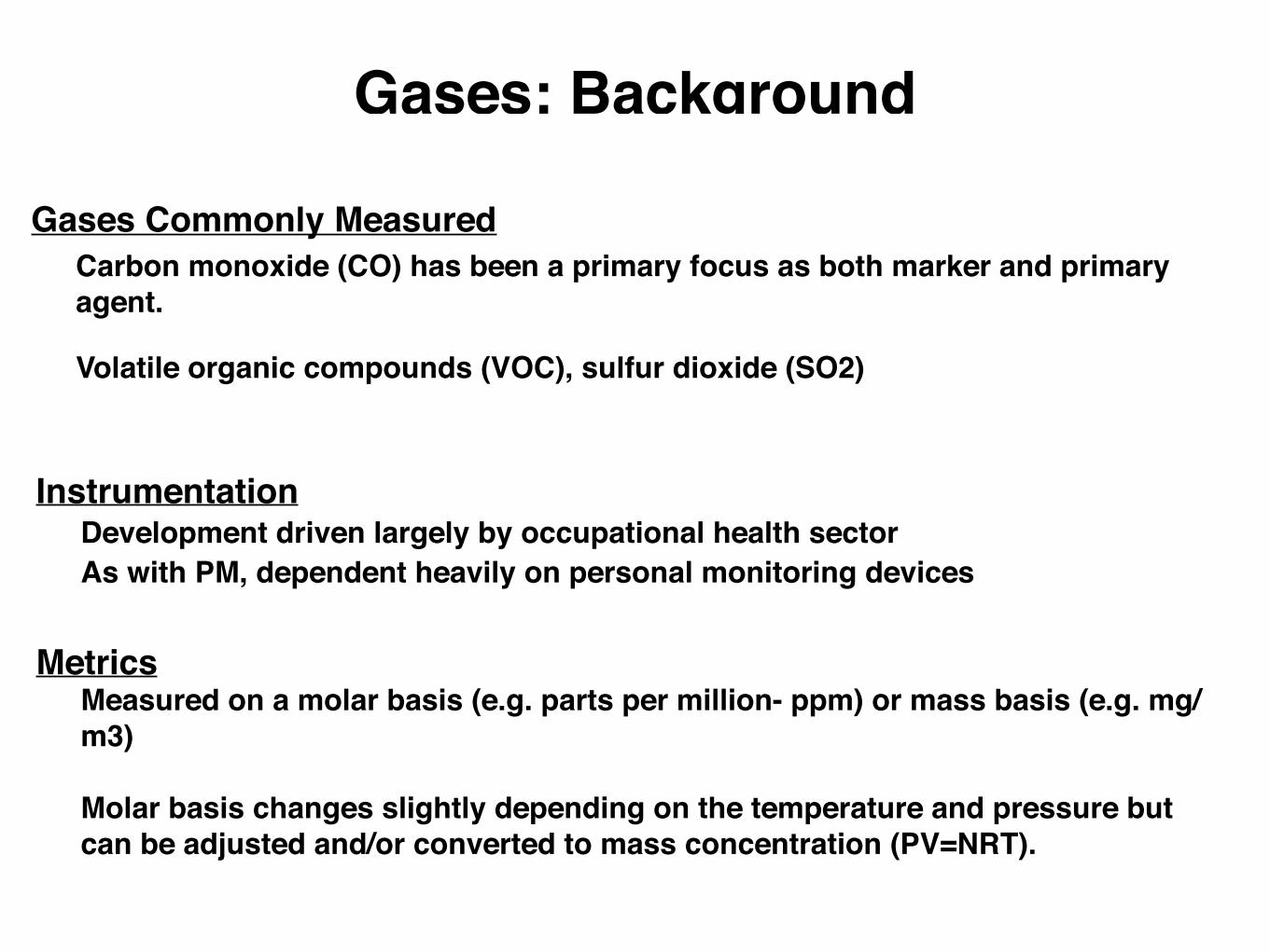
Gases: Background

Gases Commonly MeasuredCarbon monoxide (CO) has been a primary focus as both marker and primary agent.

Volatile organic compounds (VOC), sulfur dioxide (SO2)

Instrumentation Development driven largely by occupational health sector As with PM, dependent heavily on personal monitoring devices

MetricsMeasured on a molar basis (e.g. parts per million- ppm) or mass basis (e.g. mg/m3)

Molar basis changes slightly depending on the temperature and pressure but can be adjusted and/or converted to mass concentration (PV=NRT).

Gas Detection

1 2 3 4

Colorimetric Semiconducting Metal Oxide (SMO)

Electrochemical Infrared

2 3 41Semiconducting

Metal Oxide (SMO)Colorimetric Electrochemical Infrared

Colorimetric Badges

Passive Diffusion Tubes

Badges best for qualitative assessment of gas presence

Least sensitive

Tubes are a good integrated measure if response is characterized appropriately

Cross-sensitivity, temperature, humidity, reversibility can be problematic

Cheap, easy, non-invasive

1 2 3 4

ColorimetricSemiconducting

Metal Oxide (SMO) Electrochemical Infrared

17 mm

21 mm

1 2 3 4



Tin Oxide

1 2 3 4



Small, reliable, durable, cheap

Long-lasting, stable baseline, stable outputs over time

Cross-sensitivities, humidity, temperature, power requirements

Well characterized - patent in 1962

1 2 3 4



Metal oxides change their resistance based on exposure to gases in air

Operating Principles

O- O- O- O- O-

Highly negativeIncreased Resistance

1 2 3 4



Metal oxides change their resistance based on exposure to gases in air

High resistance in clean air

In the presence of CO, resistance drops

We can measure the change in resistance - related to CO concentration

Thermal cycling caveat

DIRTY AIR

Operating Principles

CO + O- –> CO2 Decreased resistance

1 2 3 4



55.0 mm

Gas Access

51.0 mm

1 2 3 4



ELECTROLYTE

CURRENT

CO + O CO

ELECTRODES

Working ReactionCO + H2O --> CO2 + 2H + 2e

Counter Reaction2H + O + 2e --> H2O

Net ReactionCO + O --> CO2

Example: Carbon Monoxide

55.0 mm

Gas Access

51.0 mm

1 2 3 4



Good resolution, available for many gases, relatively low power demand

“Reasonable Cost” - though varies widely depending on cross-sensitivities, lifespan, resolution, and range

Typically favored for field studies

Effected by humidity and temperature

Sensor drift & signal decay

55.0 mm

Gas Access

51.0 mm

Drager Pac 7000 (~$500)

Drager Pac 7000 (~$350)

Drager Pac III (~$750)

Langen CO ($1500)

TSI Q-Trak ($2700)

Inexpensive (1ppm resolution), alarms, limited settings

Slightly more robust, alarm-shutoff

Great resolution (<1ppm), low upper limit, expensive, battery life

ToxiRAE Pro CO (~$550)

1 2 3 4



Filter

Photodetector

Identify gas based on its unique IR Spectra

IR Source4.7 µm

1 2 3 4



Filter

Photodetector

No Gas - all light passes to thephotodetector

IR Source4.7 µm

1 2 3 4



IR Source4.7 µm

Filter

Photodetector

CO present - not alllight makes it to the detector

1 2 3 4



IR Source4.7 µm

Filter

Photodetector

We can quantify the relationshipbetween light at the sensor + CO

1 2 3 4



More power demand, selective, sensitive, long life time, wide measurement range

Expensive and not available in “field-ready” form for most pollutants

Susceptible to misinterpretation if not properly cleaned/maintained

Size increases (bench) to resolve lower concentrations

Sample Bag

Best for “grab samples” or short duration sampling (meals)

Many compounds could be measured

Some pollutants require significant post-processing with laboratory equipment.

Transportation of sample bags can be difficult and expensive

Tedlar or Teflon Bag

Sample Pump w/ Filter

“Calibration”: Gas

0

10

20

30

40

50

60

70

14:50 15:15

HCO 828

HCO 416

HCO 030

HCO 829

HCO 680

HCO 830

HCO 000

HCO 000

HCO 000

HCO 000

Time

PPM

CO

Vent

Sample

Gas

Calibration and/or Test Regularly: 1) Response 2) Decay time3) Accuracy

Cannot rely on manufacture “checks”

Multiple span gas concentrations ideal but one is better than none

- Lab-only devices (bronze standards) can be used but should be tested periodically with span

Simple testing chambers can be made from hardware store supplies

Calibration test results should be analyzed same-day and criteria for sensor replacement/instrument removal should be established.

1. Rise 2. Steady State

3. Decay

Parameters

Ventilation RatesIndoor pollutant concentrations are strongly influenced by the ventilation rate in the environment (recall mass-balance of room)

Measured as air changes per unit time (e.g. ACH) in units of inverse time (1/time)

Can be measured in-field using a tracer gas: (1) few competing sources at the time of measurement and (2) stable (non-reactive) over the period of sampling.

Previous efforts use CO2 (volcano experiment, pressurized canister, people) or CO (burning bucket, bag)

Protocol involved increasing the level of tracer in the room, them measuring the the slope of the logged decay curve.

y"="$0.106x"+"3.94"R²"="0.934"

y"="$0.12x"+"4.18"R²"="0.95"

y"="$0.11x"+"3.68"R²"="0.97"

1"

1.5"

2"

2.5"

3"

3.5"

4"

4.5"

0" 5" 10" 15" 20"

Ln(PPM

"CO)"

Time"(10sec"Intervals)"

Measuring in homes

Sampling PlanBudget and logistic challenges limit our ability to deploy the “ideal” sampling plan

CRECER IAP Monitoring

Extensive Monitoring

Intensive Monitoring

Personal

Group- C Toddler

Group- P Toddler

Group- N Toddler Baby

Integrated CO

Personal Area

Integrated CO

Group- C 1. Toddler 2. Mother

Group- P 1. Toddler 2. Mother

Group- N 1. Toddler 2. Baby 3. Mother

Integrated CO

Kitchen

Continuous PM2.5

Integrated PM2.5

Kitchen

Bedroom

Outdoor Kitchen

Continuous CO

Kitchen

Bedroom

Breath CO

1. Toddler 2. Mother

Instrument Placement in Homes

1.0m from outside edge of stove Represents general cooking area

~1.5 meter above the floor Relates to the approximate

breathing height of a standing woman

Standard height needed due to vertical stratification of indoor air pollutants

Floor is defined as the lowest predominant point in the kitchen

At least 1.0 meter from doors and windows when possible

Calibration & Conclusions

Calibration of monitor affects what conclusions can be made with your data

With Calibration

Absolute differences can be reported: the actual change in concentration.

“Introduction of the improved stove into the study population reduced the 48-hr average kitchen concentration from 400 ug/m3 to 50 ug/m3 (88%)”

Without Calibration

Relative differences can be reported

“Introduction of the improved stove into the study population reduced the 48-hr average kitchen concentration by 35%."

Training in Household Air Pollution and MonitoringParo, Bhutan • 21 - 25 March 2016

training in household air pollution and...

Documents