traffic forecasting for project development · traffic forecasting for project develop~ent 7. ......
TRANSCRIPT
1. Report No. 2. Government Aceo .. ion No.
FHWA/TX-89-1112-1F ----------~------4. Tille and Subtitle
Traffic Forecasting for Project Develop~ent
7. Aulholl sl
Vergil G. Stover, Duk M. Chang, Chun-Soo Chung and George B. Dresser
9. Performing Organ; zol,on Nome ond Add,e ..
Transportation Planning Program Texas Transportation Institute The Texas A&M University System
TECHNICAL REPORT STANDARD TITLE PAGE
3. Recipient's Catalog No.
6. Perfo,ming O"on, 1010 on Cod.
8. P.rlo,ming O,goni ution R.po,t No.
Research Report 1112-1F 10. Work Unit No,
11. Cont,act 0' G,ant No.
2-10-87-1112 College Station, TX 77843-3135' 13. TypeofRepo,tondPe,iodCover.d
--------------------------~ 12. Sponsoring Agency Nome and Add, ...
Texas State Department of Highways and Public Transportation
Fi nal September 1987-August 1989
Transportation Planning Di·visidn, P.O. Box 5051 Austin, TX 78763 ,
14. Sponsoring Agency Code
~----------------.-----~--------------------------~~------------------------~ IS. Supplementary Not ••
Study was conducted in cooperation with U.S. Department of Transportation, Federal I Highway Administration. Study title: Corridor Analysis Automation
16. Ab,tloet
The traditional modeling process was developed in response to the need to evaluate future transportation needs in large, rapidly growing urban areas. The process is an excellent tool for evaluation of land-use/transportation alternatives. However, it is generally recognized that such a system level must be refined for projectlevel applications. A cas.e study showed that the manual procedure follo\lJed by the Texas Corridor Analysis Group produced results which were different from the traffic assignments results using the TRANPLAN microcomputer package. A new alternative procedure for performing corridor analysis is proposed. This procedure is illustrated through a case study.
A capacity restraint procedure which equalizes the VIC ratio of groups of links which constitute compe~ing routes was developed and tested. The prototype model demonstrated that the VIC ratios of the links in each group converge toward the av~rage VIC for that g00up. Counted volumes for turning movements were not avail- \ able. Therefore, the assigned turning movements' utilizing the equalized link VIC ratio method were compared to the results using the incremental capacity restraint. procedure. The equalized link VIC proc~dure wa$ judged to produce turning movements which are more realistic than the present capacity restraint method.
17. Key WOld,
Transportation Planning, Corridor Analysis, Traffic Assignment, Capacity Restraint, Capacity Restraint Assignment
18. Oi,trlltvtiOft Steteluftt
No restrictions~ This document is availa~le to the public through the National Techni ca 1 Informati on Servi ce, Spring-field, Vir~inia 22161
19 Security Clollif. (0/ this report) 20. Seculity CIOllil. (of thit pogel 21. No, 01 Pogu 22. Price
Uncl assn; ed Unclassified Form DOT F 1700.7 18.691
I
I

TRAFFIC FORECASTING FOR PROJECT DEVELOPMENT
Research Report 1112-1F
by
Vergil G. Stover Research Engineer
Duk M. Chang Assistant Research Planner
Chun-Soo Chung Research Assistant
and
George B. Dresser Study Supervisor
Corridor Analysis Automation Research Study Number 2-10-87-1112
Sponsored by Texas State Department of Highways and Public Transportation
In cooperation with the U.S. Department of Transportation
Federal Highway Administration
Texas Transportation Institute The Texas A&M University System
College Station, Texas
November 1989

-'.
-'.
--------------------------------------------------------------------............... -
METRIC (SI*) CONVERSION FACTORS
Symbol
In ft yd ml
In2 ft2
yd2
mi2
ac
oz Ib T
floz gal ft,
yd'
APPROXIMATE CONVERSIONS TO SI UNITS When You Know Multiply By To Find
inches feet yards miles
square inches square feet square yards square miles acres
LENGTH
2.54 0.3048 0.914 1.61
AREA
645.2 0.0929 0.836 2.59 0.395
millimetres metres metres kilometres
millimetres squared metres squared metres squared kilometres squared hectares
MASS (weight)
ounces 28.35 pounds 0.454 short tons (2000 Ib) 0.907
fluid ounces gallons cubic feet cObic yards
VOLUME
29.57 3.785 0.0328 0.0765
grams kilograms megagrams
millilitres litres metres cubed metres cubed
NOTE: Volumes greater than 1000 L shall be shown in m'.
TEMPERATURE (exact)
Fahrenheit 5/9 (after temperature subtracting 32)
Celsius temperature
• 51 Is the symbol for the International System of Measurements
Symbol
mm m m km
mm2 m2 m' km' ha
g kg Mg
mL L m' m'
..
ii u
., ..
.. ..
::
APPROXIMATE CONVERSIONS TO SI UNITS Symbol When You Know Multiply By To Find
mm m m
km
mm' m' km' ha
g kg Mg
mL L
m' m'
millimetres metres metres kilometres
LENGTH
0.039 3.28 1.09 0.621
AREA
millimetres squared 0.0016 metres squared 10.764 kilometres squared 0.39 hectores (10 000 m2) 2.53
inches feet yards miles
square inches square feet square miles acres
MASS (weight)
grams 0.0353 kilograms 2.205 megagrams (1 000 kg) 1.103
millilitres litres metres cubed metres cubed
VOLUME
0.034 0.264 35.315 1.308
ounces pounds short tons
fluid ounces gallons cubic feet cubic yards
TEMPERATURE (exact)
°C Celsius 9/5 (then Fahrenheit temperature temperature add 32)
OF -40 0
I I I' I.' 'i 1
-40 -20 OC
o , iii I I 20 40 60 80
37 i 100
OC
These factors conform to the requirement of FHWA Order 5190.1A.
Symbol
in ft yd mi
in' ft· mi' ac
oz Ib T
floz gal
ft' yd'

ABSTRACT
The traditional modeling process was developed in response to the need to evaluate
future transportation needs in large rapidly growing urban areas. The process is an
excellent tool for evaluation of land-use/transportation alternatives. However, it is
generally recognized that such a system level must be refined for project-level applications.
This research reviewed and evaluated procedures for the refinement of traffic assignment
results for applications to project planning. This review included the procedures included
in NCHRP Report 255 and the corridor analysis procedure used by the Texas State
Department of Highways and Public Transportation (SDHPT) Corridor Analysis Group.
A case study showed that the manual procedure followed by SDHPT Corridor Analysis
Group produced results which were quite different from the traffic assignment results using
the TRANPLAN microcomputer package. A new alternative procedure for performing
corridor analysis is proposed. This procedure was illustrated through a case study.
A capacity restraint procedure which equalizes the v / c ratio of groups of links which
constitute competing routes was developed and tested. The prototype model demonstrated
that the v / c ratios of the links in each group converge toward the average v / c ratio for that
group. Counted volumes for turn movements were not available for use in evaluating the
assignment results. Therefore, the assigned turn movements utilizing the equalized link v / c
ratio method were compared to the results using the incremental capacity restraint
procedure contained in the TRANPLAN package. The equalized link v / c procedure was
judged to produce turn movements which are more realistic than the present capacity
restraint method.
iv

SUMMARY
This report contains the results of a study concerned with the development of traffic
forecasts for project-level analysis. A case study using US-290 in Austin, Texas, compared
the results using the subarea analysis procedures of the TRANPLAN microcomputer
package and the Texas Travel Demand Package for a mainframe computer. Both packages
produced similar results. This case study also compared the TRANPLAN results with the
results using the Texas State Department of Highways Group. None of the procedures
tested produced results which matched those of the Corridor Analysis Group procedures.
An alternative corridor analysis procedure was developed and evaluated using State
Highway 161 as a case study; the results were compared to these using the Corridor
Analysis Group procedures. The difference between the turning movements of the
alternative iterative procedure and the Corridor Analysis Group procedure averaged less
than 30%. The iterative turning movement procedure eliminated the problem of "zero"
volumes.
A theoretical procedure for estimating turning movements as a percentage of
approach volume was developed. The theoretical results were compared to actual turn
percentages using count data from the Sherman-Denison, Texas, urban area. The count
data were for the 9-hour period 7:00 a.m. to 10:00 a.m., 11:00 a.m. to 2:00 p.m., and 3:00
p.m. to 6:00 p.m. Comparison of the theoretical and observed turn percentages indicates
that the procedure may be applicable to high volume intersections.
A prototype model equalizing the volume-to-capacity (VIC) ratios of links which
comprise competing routes was developed and evaluated using the Tyler, Texas, study area
network. The procedure produced the expected results in that the link VIC ratios
converged toward the average VIC ratio for the link group. Within the project-level
analysis area, the equalized link VIC ratio method produced "better" results than the
present incremental restraint assignment procedure. The results were judged to be "better"
because there were fewer zero movements; the distribution of left turns, thru movements,
v

and right turns was also improved. The incremental method was found to produce better
results than the other restraint assignment procedures on the Tyler network. Therefore, by
implication, the equalized link V Ie ratio procedure produces assignment results which are
better than the existing restraint assignment methods.
VI
IMPLEMENTATION
Further evaluation of the alternative corridor analysis procedure should be
undertaken prior to its adoption for routine application.
Prior to implementation of the equalized link VIC ratio restraint assignment
procedure, the two following enhancements are needed:
(1) Increase in the number of link groups on which the VIC ratios are equalized,
and
(2) Programming to improve and increase the information which the user can
easily access for analysis. Further evaluation using a large network is also
suggested.
DISCLAIMER
The contents of this report reflect the views of the authors who are responsible for
the opinions, findings, and conclusions presented herein. The contents do not necessarily
reflect the official views or policies of the Federal Highway Administration or the State
Department of Highways and Public Transportation. This report does not constitute a
standard, specification, or regulation.
Vll

ABSTRACf
SUMMARY
TABLE OF CONTENTS
............................................ iv
v
IMPLEMENTATION . . . . . . . . . . . . . . . . . . . . . . . . . . . . . . . . . . . . . . vii
DISCLAIMER ........................................... vii
LIST OF TABLES ........................................ x
LIST OF FIGURES ....................................... xi
CHAPTER I. INTRODUCTION ............................. 1
The Problem ........................................ 2 System-Level Versus Project-Level Analysis . . . . . . . . . . . . . . . . . . 4 Design Accuracy ..................................... 10 Literature Review ..................................... 13
CHAPTER II. TEXAS CORRIDOR ANALYSIS PROCEDURE. . . . . . 26
General Corridor Analysis Group Procedure ................. 26 Austin US-290 Case Study .............................. 32
CHAPTER III. APPLICATION OF ALTERNATIVE PROCEDURE .. 40
Alternative Procedure ................................. 40 SH-161 Case Study in Dallas-Fort Worth. . . . . . . . . . . . . . . . . . . . 45
CHAPTER IV. TURNING MOVEMENTS ..................... 57
NCHRP Report 255 Procedures .......................... 57 Comparison of Theoretical and Counted Turning Movements . . . . . 60
CHAPTER V. RESTRAINT ASSIGNMENT USING EQUALIZED VIC RATIOS ........................................... 85
Study Procedures .... . . . . . . . . . . . . . . . . . . . . . . . . . . . . . . . . . 85 Analysis . . . . . . . . . . . . . . . . . . . . . . . . . . . . . . . . . . . . . . . . . . . . 94
viii
TABLE OF CONTENTS (Continued)
CHAPTER VI. SUMMARY, CONCLUSIONS AND RECOMMENDA-TIONS ......................... _I ••••••••••••••••••
Conclusions Recommendations ................................... .
BIBLIOGRAPHY ........................................ .
APPENDIX A: US-290 Study Worksheet Used in Corridor Analysis Group and Nondirectional Volumes on Schematic Straight-line Network ....................................... .
APPENDIX B: Intersection Volumes Along US-290 ............... .
APPENDIX C: An Example of Turning Movements at SH-161. ...... .
APPENDIX D: Turning Movement Iterative Procedure Using Lotus .. .
APPENDIX E: Turning Movement Procedures .................. .
APPENDIX F: Development of Theoretical Turning Movements ..... .
APPENDIX G: Counted Approach Volumes and Turning Movements, Turning Movements As A Percentage of Approach Volume, and Theoretical Percent Turning Movements .................... .
ix
109
109 111
113
115
118
122
124
128
153
158
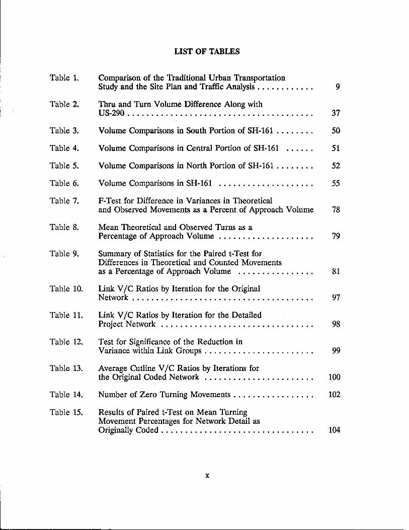
Table 1.
Table 2.
Table 3.
Table 4.
Table 5.
Table 6.
Table 7.
Table 8.
Table 9.
Table 10.
Table 11.
Table 12.
Table 13.
Table 14.
Table 15.
LIST OF TABLES
Comparison of the Traditional Urban Transportation Study and the Site Plan and Traffic Analysis . . . . . . . . . . . .
Thru and Turn Volume Difference Along with US-290 ...................................... .
Volume Comparisons in South Portion of SH-161 ....... .
Volume Comparisons in Central Portion of SH-161 ..... .
Volume Comparisons in North Portion of SH-161 ....... .
Volume Comparisons in SH-161 ................... .
F-Test for Difference in Variances in Theoretical and Observed Movements as a Percent of Approach Volume
Mean Theoretical and Observed Turns as a Percentage of Approach Volume ................... .
Summary of Statistics for the Paired t-Test for Differences in Theoretical and Counted Movements as a Percentage of Approach Volume ............... .
link VIC Ratios by Iteration for the Original Network ..................................... .
link VIC Ratios by Iteration for the Detailed Project Network ............................... .
Test for Significance of the Reduction in Variance within link Groups ...................... .
Average Cutline VIC Ratios by Iterations for the Original Coded Network ...................... .
Number of Zero Turning Movements ................ .
Results of Paired t-Test on Mean Turning Movement Percentages for Network Detail as Originally Coded . . . . . . . . . . . . . . . . . . . . . . . . . . . . . . . .
x
9
37
50
51
52
55
78
79
81
97
98
99
100
102
104
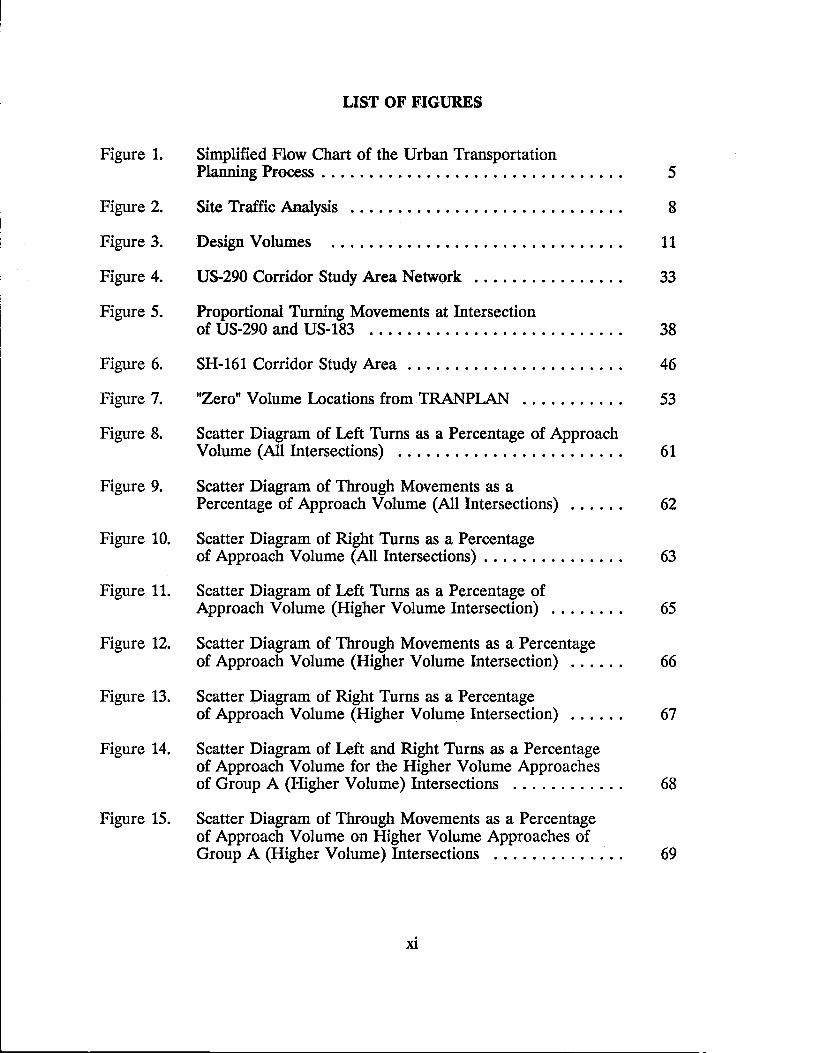
Figure 1.
Figure 2.
Figure 3.
Figure 4.
Figure 5.
Figure 6.
Figure 7.
Figure 8.
Figure 9.
LIST OF FIGURES
Simplified Flow Chart of the Urban Transportation Planning Process . . . . . . . . . . . . . . . . . . . . . . . . . . . . . . . .
Site Traffic Analysis ............................ .
Design Volumes
US-290 Corridor Study Area Network ............... .
Proportional Turning Movements at Intersection of US-290 and US-183 .......................... .
SH-161 Corridor Study Area ...................... .
"Zero" Volume Locations fromTRANPLAN .......... .
Scatter Diagram of Left Turns as a Percentage of Approach Volume (All Intersections) ....................... .
Scatter Diagram of Through Movements as a Percentage of Approach Volume (All Intersections)
Figure 10. Scatter Diagram of Right Turns as a Percentage
5
8
11
33
38
46
53
61
62
of Approach Volume (All Intersections) . . . . . . . . . . . . . . . 63
Figure 11. Scatter Diagram of Left Turns as a Percentage of Approach Volume (Higher Volume Intersection) ........ 65
Figure 12. Scatter Diagram of Through Movements as a Percentage of Approach Volume (Higher Volume Intersection) ...... 66
Figure 13. Scatter Diagram of Right Turns as a Percentage of Approach Volume (Higher Volume Intersection)
Figure 14. Scatter Diagram of Left and Right Turns as a Percentage of Approach Volume for the Higher Volume Approaches
67
of Group A (Higher Volume) Intersections ............ 68
Figure 15. Scatter Diagram of Through Movements as a Percentage of Approach Volume on Higher Volume Approaches of Group A (Higher Volume) Intersections .............. 69
xi
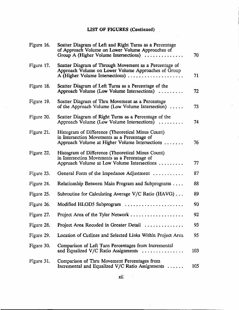
LIST OF FIGURES (Continued)
Figure 16. Scatter Diagram of Left and Right Turns as a Percentage of Approach Volume on Lower Volume Approaches of Group A (Higher Volume Intersections) .............. 70
Figure 17. Scatter Diagram of Through Movement as a Percentage of Approach Volume on Lower Volume Approaches of Group A (Higher Volume Intersections) . . . . . . . . . . . . . . . . . . . . 71
Figure 18. Scatter Diagram of Left Turns as a Percentage of the Approach Volume (Low Volume Intersections) ......... 72
Figure 19. Scatter Diagram of Thru Movement as a Percentage of the Approach Volume (Low Volume Intersection) ..... 73
Figure 20. Scatter Diagram of Right Turns as a Percentage of the Approach Volume (Low Volume Intersections) ......... 74
Figure 21. Histogram of Difference (Theoretical Minus Count) in Intersection Movements as a Percentage of Approach Volume at Higher Volume Intersections. . . . . . . 76
Figure 22. Histogram of Difference (Theoretical Minus Count) in Intersection Movements as a Percentage of Approach Volume at Low Volume Intersections . . . . . . . . . 77
Figure 23. General Form of the Impedance Adjustment ........... 87
Figure 24. Relationship Between Main Program and Subprograms . . . . 88
Figure 25. Subroutine for Calculating Average VIC Ratio (HA VG) . . . 89
Figure 26. Modified HWD5 Subprogram ..................... 90
Figure 27. Project Area of the Tyler Network. . . . . . . . . . . . . . . . . . . 92
Figure 28. Project Area Recoded in Greater Detail .............. 93
Figure 29. Location of Cutlines and Selected links Within Project Area 95
Figure 30. Comparison of Left Turn Percentages from Incremental and Equalized VIC Ratio Assignments ............... 103
Figure 31. Comparison of Thru Movement Percentages from Incremental and Equalized VIC Ratio Assignments
xii
105
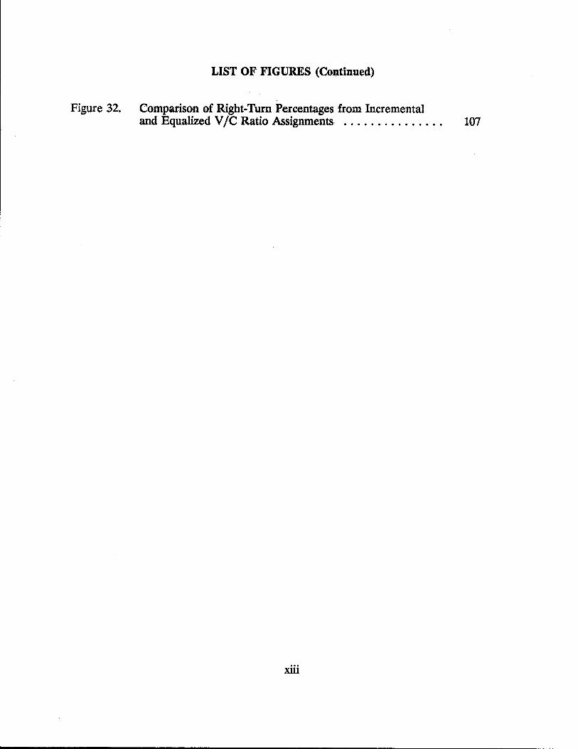
LIST OF FIGURES (Continued)
Figure 32. Comparison of Right-Turn Percentages from Incremental and Equalized V Ie Ratio Assignments ............... 107
xiii
CHAPTER I. INTRODUCTION
The modeling process utilized in urban transportation studies was developed in
response to the need to evaluate future transportation needs in large rapidly growing urban
areas. This computerized modeling procedure is effective for system-level analyses involving
the evaluation of land-use/transportation alternatives, the compatibility of given land-use
and transportation scenarios, the identification of travel corridors and the approximate
volume of future traffic in each corridor, and staging of major transportation system
improvements in response to projected urban growth. Thus, the traditional transportation
modeling process has been found to be an excellent tool for system-level analysis and policy
evaluation.
The modeling process is also applicable to statewide and large regional studies.
Further, it has been successfully used in a variety of other applications such as the Texas
Airport System Study (1).
The desire to analyze portions of a large urban region in greater detail than the
system-level analysis allows has lead to subarea studies. Thus, windowing and subarea
focusing procedures were developed to allow the analyst to make changes in the land-use
and/or the transportation system within the subarea of interest. These procedures permit
the analysis of localized alternatives within the subarea while maintaining the regional
context in which the subarea is situated. It also minimizes the data set which must be
manipulated, and it substantially reduces the computer time needed. Each windowing and
subarea focusing technique has been incorporated in the Texas Travel Demand Package as
well as various other computer packages. Through Study No. 2-10-87-1110, "Subarea
Analysis Using Microcomputers," procedures and software were developed so that the
subarea analysis could be performed on a microcomputer and interfaced with the Texas
Travel Demand Package on the SDHPT mainframe computer. While using greater network
detail than the system-level studies, the subarea analysis utilizes the same trip generation
and trip distribution models.
The models used in the Texas Travel Demand Model (as well as other mainframe
packages such as UTPS and the various microcomputer packages such as TRANPLAN,
Micro TRIPS and MINUTP) involve a variety of simplifying assumptions. These
1
assumptions are necessitated by the complex combination of a large number of factors
involved in individual travel behavior. Consequently, estimates of base-year traffic on
individual facilities in a system-level analysis can differ significantly from the actual counts.
This may be the case even when it is recognized that one- or two-day short counts produce
average daily traffic (ADT) estimates which may have about an 80% probability of being
within ± 15% of the true ADT (2). Where there are multiple facilities within a corridor,
the error in the total corridor volume will be much less due to the offsetting errors on the
individual facilities. Furthermore, the precision necessary in system-level analysis is the
difference in the capacity of 2 vs. 4 vs. 6 vs. 8 lanes or about 15,000 for an arterial street
and about 40,000 for a freeway.
THE PROBLEM
More detailed uses and needs for traffic forecasts involve project-level applications
including the following:
1. Design of route-segments (including ramps, interchanges, and intersections)
which are maintained by the SDHPT. These "on-system" roadways consist
of all the freeways and many of the major at-grade streets within urban areas,
the majority of which are the urban extensions of state highways and
farm/ranch-to-market roads.
2. Design of major street segments other than those facilities on the SDHPT
maintained system (e.g., the off-system facilities). These off-system facilities
are a municipal or county responsibility. They interconnect with the on
system roadways and are, therefore, of some interest to SDHPT.
3. Site traffic impact studies for proposed urban development projects which
may range from a few dwelling units to mixed use development consisting
of several million square feet. Such projects range in size from small to
large. Large projects will influence intersections some distance from the site.
Also, large projects are likely to be located with access to on-system facilities.
4. Site access and circulation design of proposed urban development projects;
including drive-through length and width, curb return radii, channelization,
2
and future traffic control. Commercial and industrial developments and larger
residential subdivisions are likely to have access to an on-system roadway.
Such projects range in size from small to large.
5. Intersection design; including number of lanes, number and length of left
turn bays, length of right-turn bays, curb return radii, channelization, and
future traffic control.
6. Expected speed, delay, queue length.
7. Effect of proposed changes in land use.
8. Effect of multiple closely spaced access drives as opposed to fewer better
designed access points.
9. Geometric design for large trucks.
10. Pavement design.
The application identified in the item 1 above, design of on-system facilities, is of
obvious concern to SDHPT. Site traffic generation and site access and circulation design
are of major concern to municipalities, and in states other than Texas, to counties as well
as to the developers of the projects. However, there is an increasing concern for these
applications in those SDHPT districts which contain expanding urban areas. This concern
comes from the recognition that traffic generated by urban development impacts the on
system facilities, even though the development may not directly front or have direct access
to an SDHPT-maintained facility.
When a large traffic generating project is involved, the area of influence will be
considerable and will impact intersections and interchanges which are some distance from
the site. The location and design of the access will directly impact the adjacent public
street, especially nearby intersections and/or interchanges. Therefore, the SDHPT interest
in project-level applications extends beyond the design of on system facilities.
Irrespective of the user, the first eight project-level applications share a common
problem. That is, the need for detailed traffic projections which provide individual
movements (i.e, left, right, and thru movements at intersections) by time of day.
Design for large trucks, the item 10 above, can be categorized into three situations:
(1) "site-specific" development such as truck terminals and industrial areas; (2) truck routes
through towns and cities; and (3) freeway and street design in general.
3
SYSTEM-LEVEL VERSUS PROJECT-LEVEL ANALYSIS
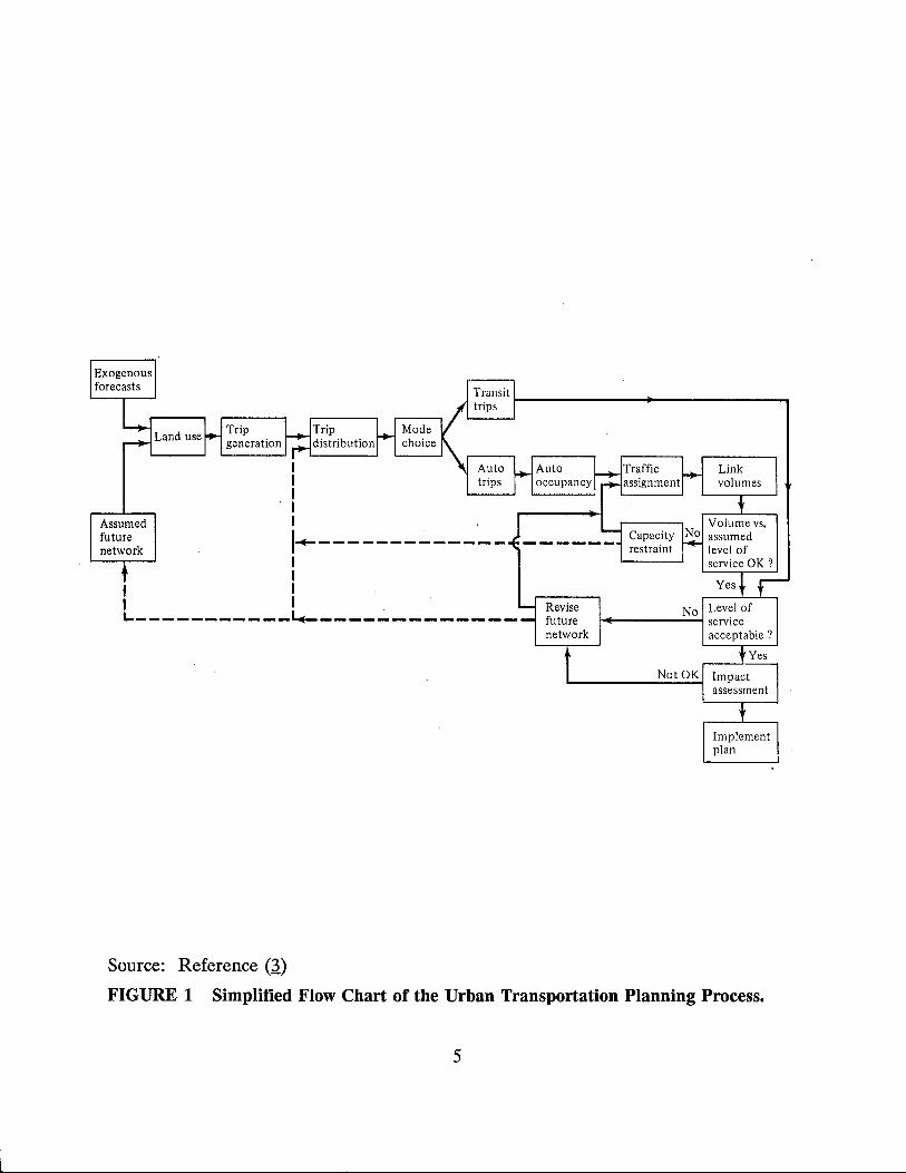
A simplified flow chart of the traditional urban transportation planning process is
given in Figure 1. As previously indicated this process was developed to evaluate future
land-use/transportation alternatives. The process is also an excellent tool for the following:
1. Identifying major travel corridors and the approximate future traffic volume
within each corridor given a future land-use arrangement.
2. Identifying potential major problems in a proposed network given a future
land use or evaluating a proposed land-use arrangement given a future
transportation network.
3. Providing a basis for planning and programming major transportation network
improvements.
The process provides information (mean trip length and trip length frequency) by
which the compatibility of the proposed land-use plan and the proposed transportation
plan can be evaluated. It can also be used to evaluate the relative accessibility of the
existing land-use/transportation pattern, to identify changes in accessibility that would
result with different transportation systems, and to see if proposed large commercial or
industrial concentrations are situated at locations which have, or will have, a high level of
accessibility.
The urban transportation modeling process, which relies heavily upon computer
models, is a macroscopic tool which uses an abstract computerized representation of the
street and highway network in the traffic assignment. The results are not directly suitable
at the microscopic or site planning level because it does not provide
1. Reliable forecasts of turning movements at individual intersections or access
drives;
2. Time of day projections of the traffic volumes on individual street segments;
3. Reliable forecasts of traffic volumes at access drives for different access
locations and/or designs;
4. The effect of numerous access points to an arterial as opposed to only a few
direct access points;
4
Assumed future network
I I I I I
~-------~-----I I
I I I I. .
~-----------~-------------
Source: Reference (~)
Revise future network
No
FIGURE 1 Simplified Flow Chart of the Urban Transportation Planning Process.
5

5. Effects of minor changes in land use;
6. Effects of modest changes in the location of activities; e.g., the positioning
of 250,000 square feet of retail floor area on each of the 4 quadrants of an
intersection versus the location of all 1 million square feet in one quadrant;
and
7. Reliable forecasts of the traffic on the frontage roads separate from that or
the main lanes of a freeway or at-grade arterial.
Both the urban general (comprehensive) planning process and the urban
transportation planning process commonly utilize a single 20-year time horizon. In order
to deal more effectively with transportation and land-use development, there is growing
recognition that the planning process should be stratified into the following four planning
horizons or level:
1. Level 1: An infinite, or at least a very long, horizon for strategic planning
of major transportation corridors and other permanent elements of the urban
environment.
2. Level 2: A long-range horizon (20 years) for the planning of significant
changes in transportation facilities, water, waste water, and other major
infrastructure elements and land-use patterns.
3. Level 3: A medium-range horizon (3 to 5 years and 10 years for very large
capital improvement projects) for planning, programming, and design of
major development.
4. Level 4: A short-range horizon (commonly one year) for the approval of
individual construction contracts for public improvements and private
development projects.
The successive stages should constitute a progression of planning design with an
increasing degree of refinement and detail at each successive stage.
The Level 1 and 2 plans should provide general policy guidance for public and
private development decisions. These are the shortest time horizons for which direct
application of the urban transportation modeling process was intended. Level 3 needs to
provide effective coordination of public sector infrastructure decisions and coordination
6
between the public sector and private sector development decisions. Level 4 deals with
the funding of individual construction contracts.
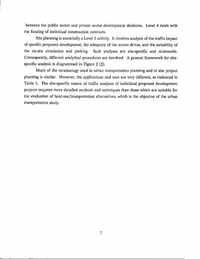
Site planning is essentially a Level 3 activity. It involves analysis of the traffic impact
of specific proposed development, the adequacy of the access drives, and the suitability of
the on-site circulation and parking. Such analyses are site-specific and microscale.
Consequently, different analytical procedures are involved. A general framework for site
specific analysis is diagrammed in Figure 2 (~).
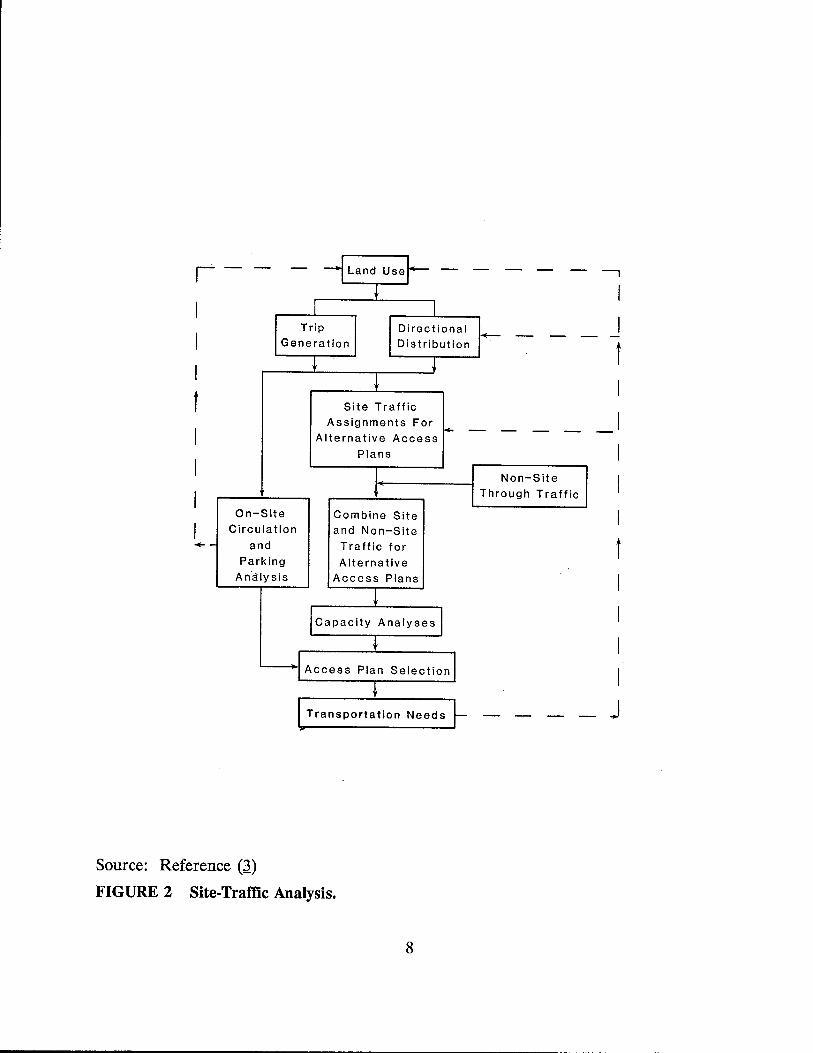
Much of the terminology used in urban transportation planning and in site project
planning is similar. However, the applications and uses are very different, as indicated in
Table 1. The site-specific nature of traffic analyses of individual proposed development
projects requires more detailed methods and techniques than those which are suitable for
the evaluation of land-use/transportation alternatives, which is the objective of the urban
transportation study.
7
I
I I I
t
-
- - - Land Use - - - - -t
I Trip Directional t-- - -Generation Distribution
t t t
Site Traffic Assignments For
1+ - - - -Alternative Access
Plans
I Non-Site
~ Through Traffic
On-Site Combine Site Circulation and Non-Site
and Traffic for Parking Alternative
An111ysis Access Plans
1 Capacity Analyses
~ I LAccess Plan Selection I
1
I
t
I
t
l Transportation Needs ~ - - - - j
Source: Reference GD FIGURE 2 Site-Traffic Analysis.
8
TABLE 1 COMPARISON OF THE TRADITIONAL URBAN TRANSPORTATION STUDY AND THE SITE PLAN AND TRAFFIC ANALYSIS
Analysis Element
Mode choice
Trip distribution
Traffic assignment
Use of results
Urban Transportation Planning Study
Interzonal and intrazonal trips generally are obtained with gravity model using zone-to-zone, and intrazonal travel times obtained by trip generation.
Person trips are "split" into auto and transit - generally using some mathema~ical model. The auto mode trips are then converted to auto/vehicle trips using auto occupancy factors. In urban areas where there is little or no transit, auto/vehicle trips and transit trips (if any) are most appropriately obtained by direct generation.
Zone-to-zone movements obtained using a gravity model calibrated for the urban area.
Zone-to-zone trips assigned to the coded, abstract network using minimum paths, all-or-nothing, or multiple-path "capacity" restrained assignment.
Assess the internal consistency of a land use-transportation plan.
Evaluate and compare mutually exclusive land use-transportation plans.
Identify major problem areas in the transportation plan given a land use plan.
Identify movement corridors and project the approximate volume within each corridor.
Identify major system deficiencies in the existing transportation system in comparison to the adopted land use-transportation plan.
Source: Reference (~) 9
S,ite Plan and Traffic Analysis
commor)ly used trip-generation rates are auto trips.
Trips are projected by direction: into the development (destination) or out from the development (origin).
When a large development is mixed-use (e.g., retail and office), the number of trips to and from the site must be adjusted.
Where some of the trips are expected to be made by transit, the number of transit trips is projected and the number of auto trips is reduced using auto occupancy rates.
Percentage of traffic to/from the site obtained by: (1) geographical distribution of clientele within the primary trade zonesmanual analysis using judgment, or (2) gravity model application - computerized or manual methods, or (3) analogyappropriate in situations where a similar business is already located in close proximity to the proposed development.
Percentage of traffic using each access point is projected. Traffic volume at each access point by movement. Traffic added by the proposed development projected by movement for each street segment and intersection adjacent to and within the traffic influence area of the proposed development. If computerized, thorough, detailed analysis of the results is essential.
Identify the selected peak-hour demands at individual access points of a proposed development.
Assess the capacity of the proposed access and its adequacy to accommodate the projected demand.
Evaluate the layout of the on-site circulation and parking, building location, and location and design of the access in relation to the adjacent street(s).
Identify the need for street improvements such as additional through lanes, turn lanes, and traffic control adjacent to and within the area of traffic influence of the proposed development.
DESIGN ACCURACY
It is common practice to estimate the average annual daily traffic (AADT) or
average annual weekday traffic (A WDT) from traffic counts which are made for a short
time (one or two days). These short counts provide estimates which are within about 10%
or 15% of the actual AADT or A WDT with about 80% confidence. It is not logical to
interpret traffic assignment forecasts as having greater accuracy than the precision with
which existing traffic is counted.
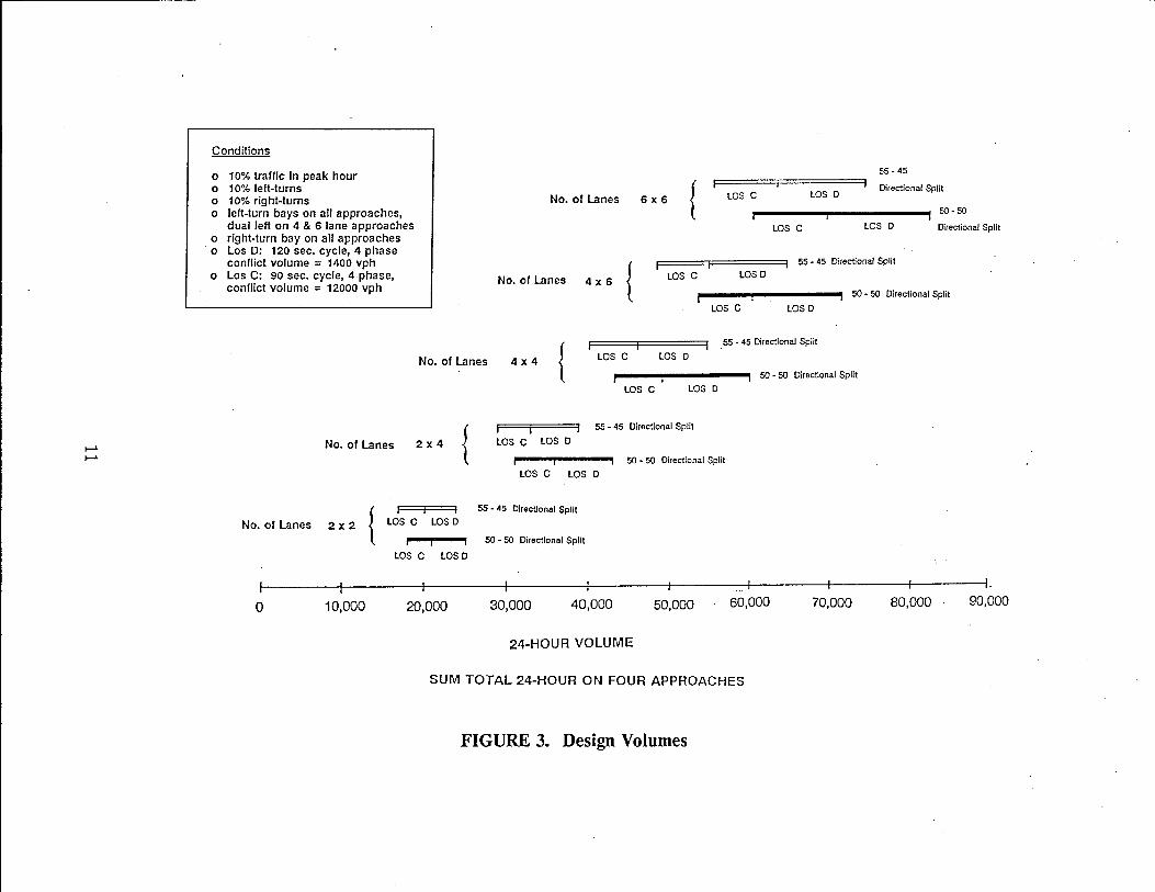
Moreover, when interpreting traffic application, it is important to note that volume
is, essentially, a continuous variable (traffic volume can be measured in increments of one
vehicle). Capacity, on the other hand, can be provided only in large increments, i.e., one
lane per approach. Figure 3 illustrates the maximum theoretical capacity provided by
intersections having a different approach cross section. A 2 x 2 intersection is one at which
all four approaches have a single thru lane (i.e., the intersection of two 2-lane undivided
roadways). A 4 x 4 is the intersection of two 4-lane divided roadways (all four approaches
have two thru lanes). The conditions assumed in calculation of the two capacities are as
follows:
1. 10% of the 24-hour traffic carried in the peak hour (highest volume 60
minutes).
2. 10% left turns.
3. 10% right turns.
4. Separate left-turn and right-turn bays provided on all four approaches; dual
left-turn bays assumed on all 4-lane and 6-lane facilities.
5. LOS D: 4-phase signal, 120-second cycle, maximum conflicting volume of
1,400 vph.
6. LOS C: 4-phase signal, 90-second cycle, maximum conflicting volume of 1,200
vph.
7. LOS B: 2-phase signal, 60-second cycle, maximum conflicting volume of 1,060
vph.
10
Conditions
o 10% traHic In peak hour o 10% left-turns o 10% right-turns o left-turn bays on all approaches,
dual left on 4 & 6 lane approaches o right-turn bay on all approaches o Los D: 120 sec. cycle, 4 phase
conllict volume = 1400 vph o Los C: 90 sec. cycle, 4 -phase,
conllict volume = 12000 vph
No. of Lanes
No. of Lanes 4 x 6 { LOse
LOS e LOSD
LOse
55 - 45
Directional Split
LOS D
50·50
Directional Split
55 - 45 Directional Split
LOS D
50 - 50 Directional Split
LOS e LOS D
_ 55 - 45 Directional Split
No. of Lanes 4 x 4 { LOse LOSD
,...--.,..----.-.0111 50·50 Directional Split
LOS e LOSD
1 I 55 - 45 Directional Split
No. of Lanes LOSe LOSD
50 - 50 Directional Split
LOS e LOS D
{ I I 55 - 45 Directional Split
No. of Lanes 2x2 lOS e LOS D
50 - 50 Directional Split
LOSe LOS D
~-------4---------+1---------+--------~--------~1---------+1--------41---------+I------~I.
o 10,000 20,000 30,000 40,000 50,000 60,000 70,000 80,000 90,000
24-HOUR VOLUME
SUM TOTAL 24-HOUR ON FOUR APPROACHES
FIGURE 3. Design Volumes
The figure presents the capacity ranges for a 55/45 directional split and a 50/50
directional split. The 55/45 split probably represents a practical design condition, whereas
the 50/50 split represents an optimistic or maximum physically possible condition.
The upper limits of LOS D are about 15% greater than the upper limits of LOS C
(the boundary between LOS C and LOS D). This is approximately the error associated
with traffic counts. This suggests that designing for LOS D is a questionable practice. A
desirable practice is to design for the next larger intersection configuration when the
forecast traffic assignment is within the LOS D range. For example, if the total assigned
traffic on the four approaches is greater than about 46,000, the design should be an
intersection of a 4-lane street with a 6-lane street rather than the intersection of two 4-
lane streets. Depending upon the forecast traffic at other major intersections, the 6-lane
cross section may be configured for a substantial distance or the cross section may be
"flared" from 4 lanes to 6 lanes at the intersection in question.
An obvious characteristic shown in Figure 3 is the gap between the intersection of
two 2-lane streets and the intersection of a 2-lane and a 4-lane divided street. As an
extension of the preceding paragraph, when the total forecast 24-hour approach volume is
more than 18,000 or 20,000 vpd, at least one of the intersection streets should be designed
with 4 lanes (or flared to 4 lanes) at the intersection.
In some cases there is no overlap of the LOS D capacity and the LOS C capacity
of the next larger intersection configuration (see Figure 3). For example, the upper limit
of LOS D of a 2-lane street with a 4-lane street is about 39,000 vpd (for a 55/45 directional
split). The LOS C capacity for an intersection of two 4-lane streets begins at about 40,000
vpd, whereas there is a substantial overlap between 4 x 4 and 4 x 6 as well as the 4 x 6 and
6 x 6 intersection configurations.
12
LITERATURE REVIEW
System-level traffic data is not appropriate for project-level analysis and design.
Therefore, an analyst must take the system-level data and manually reassign the traffic to
a detailed schematic network representing all roadways and intersections within the corridor
(project area) of interest. Such procedures are time consuming, costly and require
considerable judgment on the part of an experienced analyst. Consequently, the results are
not reproducible (at least not easily reproducible) by different analysts.
NCHRP Report 255
The National Cooperative Highway Research Program sponsored research which
produced an exhaustive study of procedures to translate system-level traffic assignment
results into traffic data needed for individual highway project use (1). This project included
the following three tasks:
1. Investigate procedures being used to develop data for project planning and
design;
2. Develop and recommend appropriate procedures for the range of planning
and design needs; and
3. Prepare a user's manual with illustrative case studies.
NCHRP Report 255 provides a good synthesis of the procedures that work best for
developing project-level data from traffic assignments. This report represents the only
major effort (1) in documenting standardized procedures that produce traffic data for use
in project planning and design, (2) in establishing accepted procedures that translate various
inputs into project traffic data, and (3) in specifying the contents, accuracies, and limitations
of the data for the problem being addressed. The following general conclusions were
presented in this report based on the finding of the research:
1. Traffic data are used for three primary purposes in highway project planning
and design:
(a) for evaluation of alternative highway improvement projects;
13

(b) for input to air quality, noise, and energy analyses of highway
improvement projects; and
(c) for input to capacity and pavement analyses.
2. The traffic assignments that are produced by system-level computerized traffic
assignment procedures must, in virtually all cases, be refined and subjected
to further analysis in order that traffic data can be produced which can be
used for highway project planning and design.
3. Until now there has been virtually no national standardization of procedures
for the development of traffic data that are used as input to evaluation and
environmental and design analyses. As a result, there are wide variations in
the format and quality of traffic data produced by agencies.
4. Production of adequate traffic data requires considerable effort and time as
well as judgment that comes with experience.
5. A large number of explicit assumptions are made every time traffic forecasts
are performed for project planning and design studies.
6. It is important that the analyst applying the procedures have a general
understanding of how the traffic data are to be used to insure that the proper
data are prepared.
7. The users of the traffic data must understand the limitations and degree of
uncertainty associated with traffic forecast data.
The appendix to NCHRP Report 255 is a user's guide which presents procedures
for different applications on data needs. These, together with a brief statement of the
purpose and methodology of each are as follows:
1. Preliminary Checks of Computerized Traffic Volume Forecasts
Purpose: To check the necessity of further refinement for the traffic
forecasts.
Check 1:
Check 2:
Check 3:
Check 4:
Examine the traffic forecasts with land use data assumptions.
Compare future trip end summary to land use data assumptions.
Examine highway network assigned by the future year traffic
forecasts.
Compare base year traffic count with the assigned volume of the
14
Check 5:
base year.
Compare the traffic forecasts with growth trends oflink volumes,
VMT, population, employment and households
2. Refinement of Computerized Traffic Volume Forecasts
Purpose: To document procedures that will allow for the refinement to
take place in a rational and consistent manner.
(a) Screenline Refinement Process
Input data: Highway network with historical record, base year traffic
counts, base year assignment, base year link capacity, and land-use
growth trends
Procedure: Select screenline ---- > check base year volume ---- >
perform computation ---- > enter available data onto the calculation
form ---- > calculate adjustments due to base year assignment deviation
---- > calculate %TCOUNT, %GCf, RAf/Cf and COUNT ICb ---- >
perform final checks
(b) Select Link Analysis
Input data: Historical record network and trip table, future year traffic
assignment
Procedure: Determine key links within the study area ---- > prepare
input data, run program, and check output ---- > place output into
refinement format ---- > identify inconsistencies and errors ---- > make
refinement to traffic assignment
3. Traffic Data for Alternative Network Assumption
Purpose: To enable alternative highway projects to be effectively
evaluated.
Application: Changes in roadway capacity, construction of parallel roadways,
change in roadway alignment, and addition or deletion of
roadway links.
(a) Modified Screenline Refinement Procedure
Application: For examining changes in roadway capacity and
construction of parallel facility
15
Procedure: Apply screenline procedure for original future year
network ---- > repeat procedure using revised network data ---- >
compare assignment --- > perform reasonableness check ---- > make
final adjustment
(b) Modified Select Link/Zonal Tree Analysis
Application: For analyzing different roadway alignments, construction
of parallel facilities, or the addition/subtraction of roadway links
Procedure: Refine assignment for original future year network ---- >
estimate magnitude of network change ---- > determine link or
zones for analyzing network changes ---- > perform appropriate
computer run ---- > identify competing paths and compute new travel
time ---- > perform volume adjustment ---- > make final check of
volume/capacity ratio
4. Traffic Data for More Detailed Networks
Purpose: To produce a traffic assignment on a detailed highway network
using available data.
Method: Subarea windowing, subarea focusing
Input data: Trip table, network, zonal land use, appropriate computer
software
Procedure: Define study area ---- > define new zone system and highway
network ---- > define trip table for revised network ---- > assign
trips to revised network ---- > refine trip assignment within study
area
5. Traffic Data for Different Forecast Years
Purpose: To produce traffic data for a target year that is different from
that used in any computer forecasts.
Input data: Land-use projection, patterns of land use and traffic growth,
staging of highway and transit facilities, available capacity of the
roadway system, historical traffic trends, timetable of land-use
development, and future year forecasts
Growth: Linear (uniform) or nonlinear (increasing growth decreasing
16
growth, or stepped growth)
( a) Interpolation Method
For estimating traffic between two future year assignment, needs two
sets of known values between which data can be generated
Procedure: Select assignments to bracket the desired year ---- >
determine the shape of the growth curve ---- > calculate interpolation
factor ---- > perform computation
(b) Extrapolation Method
For estimating traffic for years beyond any available traffic forecast
for years within a short time frame from the base year or when only
one adequate traffic forecast is available
Procedure: Select forecast ---- > determine the shape of the growth
curve ---- > calculate extrapolation factor ---- > perform computation
6. Turning Movement Procedures
Purpose: To enable the analyst to develop the future year assignment of
the turning movement.
Input data: Future year turning volume forecasts, directional and
nondirectional volume forecasts, actual base year turning
movement counts, desired time period, and number of
intersection approaches
(a) Factoring Procedures: ratio method, different method, and combined
method
(b) Iterative Method: directional volume method and nondirectional
volume method
(c) liT' intersection procedures: nondirectional turning movement method
and directional turning movement method
7. Design Hour Volume and Other Time of Day Procedures
Purpose: To forecast design hour volumes and peak hour factor.
(a) Design Hour Volume (DHV)
Objective: To select a specific hour of future traffic volume that will
be used as the basis for design
17
"'------------------------------------------------
Method: The hour at which the slope of the traffic volume curve
changes most rapidly -- the 30th highest hour of the traffic volume
curve
Result: 8%-12% of ADT (work travel), 12%-18% of ADT
(recreational travel)
(b) DHV Forecasting Procedures for Typical Urban Facilities
Identify highway facility characteristics ---- > select a PHT / ADT ratio -
--- > multiply the PHT / ADT ratio by the future ADT
( c) Peak Hour Factor
Definition: The ratio of the traffic carried during the peak 5-minutes
of the peak hour to the total traffic carried during the peak hour (for
freeways and expressways), the ratio of traffic carried during the peak
15 minutes of the peak hour to the total traffic carried during the peak
hour (for arterials)
8. Directional Distribution Procedures
Purpose: Expecting the future change in directional distribution
( a) Procedure using modification of base year data
Input data: Future year traffic directional distribution, base year
traffic distribution, future year work trip directional distribution, and
base year work trip directional distribution
Procedure: Obtain estimate of the year directional distribution of peak
hour traffic ---- > determine the directional distribution of home to
work travel in the base and future year ---- > establish the
reasonableness of base year estimated peak hour traffic directional
distribution given the base year work travel directional distribution -
--- > forecast future year directional distribution by factoring base year
directional distribution
(b) Procedure using anticipated future conditions
Input data: Future year forecasted peak hour traffic, estimated future
year facility characteristics, and base year directional distributions on
facilities with similar characteristics to those of future facility
18
L-_________________________________________________________________ _
Procedure: Identify the highway facility characteristics which influence
directional distribution and the degree of influence of each
characteristic ---- > select a peak hour directional distribution based
on the anticipated characteristics of the facility ---- > multiply the future
estimated peak hour directional distribution by the future year peak
hour total traffic
( c) Procedure to adjust intersection directional link volumes
Input data: Hourly directional link volume on each approach
Procedure: Check volume totals ---- > calculate the difference between
the inbound and outbound movements ---- > adjust the total inbound
trips among approaches ---- > calculate adjusted outbound movements
for each hour ---- > make final check
9 . Vehicle Classification Procedures
Purpose: To forecast the vehicle classification of the future year.
Usage: Capacity analysis, pavement design, and environmental analysis
Consideration: The effects of forecasted land-use changes, long term vehicle
classification counts
Procedure: Select base year vehicle classification ---- > compare base year
and future year land use ---- > estimate the future year vehicle
classification
10. Speed, Delay and Queue Length Procedures
Purpose: To calculate the future speed, delay and queue length.
Definition: Average speed, average running speed, operating speed, design
speed queue and delay
Consideration: Under-capacity and over-capacity
(a) Speed procedure:
Input data: Design speed and volume-to-capacity ratio
Procedure: Apply design speed and volume-to-capacity ratio
relationships to estimate average running speed ---- > convert average
running speed to operating speed
(b) Speed and delay procedure:
19
Input data: Signal cycle length, approach volume, flow rate, green
time, green-to-cycle time ratio capacity
Procedure: Determine the mid-block average running speed ---- >
calculate intersection delay on each of the facility approaches ---- >
calculate total intersection delay on each of the facility approaches
(c) Queue length calculation procedures:
Input data: Approach flow rate, degree of saturation, cycle length,
green-to-cycle time ratio
Procedure: Estimate the average proportion of vehicles stopping
during a signal cycle ---- > calculate the average queue length
11. Traffic Data for Design of Highway Pavements
In addition, the following three case studies are presented:
1. Use of refinement procedures for upgrading a limited access highway.
2. Use of windowing procedures for evaluating an arterial improvement.
3. Application of procedures for highway design.
The researchers recommend the following six areas of research:
1 The development of microcomputer of several procedures in a user's manual.
2. A need to better quantify factors influencing traffic growth.
3. A noniterative procedure to derive directional turning volumes to increase
its applicability and to simplify its calculation.
4. Improved relationships between various highway speed groups.
5. An improved statistical base for transferring time-of-day, directional
distribution, and vehicle classification data.
6. Quantifying truck time-of-day relationships.
A significant deficiency with the procedures presented in NCHRP Report 255 is that
while it is suitable for a single intersection, the procedure is weak and very complex when
applied to several intersections.
20
S.I.T.E. Handbook
The project-level traffic data desired for the traffic impact evaluation and design of
proposed development includes individual movements (left, right, and thru) at all access
drives to the proposed development, at all existing and proposed intersections adjacent to
the proposed development, and at all intersections within the development areas of traffic
influence. Procedures to develop such detailed project-level traffic data are presented in
a report prepared for the Federal Highway Administration, Report No. FHWA/PL/85/105,
"Site Impact Traffic Evaluation (S.I.T.E.) Handbook" (In. This report is available through
the Institute of Transportation Engineers.
This manual presents analytical procedures (with examples) for the projection of
traffic volumes by movement that will be generated at each access drive and intersection
adjacent to and within the development's area of traffic influence. Such detailed project
level data are necessary to (a) access the traffic impact on the street system and nearby
intersections, (b) evaluate the location and design of the proposed access drives, ( c)
evaluate the need for and effectiveness of changes in traffic operations and control of
existing intersections within the area of traffic influence of the development, and (d)
evaluate the need for and effectiveness of alternatives for the redesign of existing and
proposed intersections within the area of traffic influence.
The procedures as presented in the S.I.T.E. Handbook are for manual calculations.
However, consulting firms have developed microcomputer programs to assist in making
the calculations, and various proprietary software packages are available.
Other Research
Eash, Janson, and Boyce (2) investigated the advantages and implications for practice
of equilibrium trip assignment. The authors concluded that equilibrium trip assignment,
rather than iterative assignment, should always be used on large networks especially for
congested networks. They remarked that the method which best replicates the observed
vehicle flows may depend on the detail of the network, the accuracy of the capacity-restraint
functions, and the time period of the assignment. Finally, the authors concluded that the
21
use of equilibrium assignment to produce 24-hour assignments may be inappropriate in that
only the peak periods have truly congested flow. All-or-nothing assignments may be
sufficient for off-peak periods.
Creighton and Hamburgh (10) developed a micro-assignment for simulating detailed
vehicular movements in small areas. Unlike region-wide assignment approaches, this model
has the ability to assign traffic to a finely coded street network for various time periods
throughout the day. The time periods can be of short enough duration to reflect congestion
realistically and are limited only by the practitioner's ability to obtain assigned trips by short
time periods. Most O-D (origin-destination) surveys have time reported to the nearest one
tenth of an hour (six minutes).
Research by Stover, Woods, and Brudeseth (11) found that the application of
volume-to-capacity relationships contained in the "Highway Capacity Manual," TRB Special
Report 87. to traffic assignment produces "wide swings" in the impedance and assigned link
volumes from one iteration to another. They concluded that the speed and VIC
relationship used in traffic engineering was not applicable to traffic assignment. The
researchers found that some "dampening" needed to be applied in order to achieve
convergence in a capacity restraint assignment.
Benson and Cunagin (12) investigated the effects of implementing various impedance
adjustment functions that could be applied to all over- or undercapacity links between each
iteration on capacity restraint assignment. They concluded that the currently used capacity
restraint functions are similar. The Bureau of Public Roads (BPR) function was found to
be the most appropriate impedance adjustment function. The authors indicated that there
were several problems with respect to developing capacity adjustment functions in the
application of speed-flow relations in the assignment process. These problems occur for two
reasons: (1) the most critical flow problems actually occur over short time spans, and (2)
the assignment process may load a facility far in excess of capacity based upon some
originally coded speed, but observed conditions are limited to some maximum capacity. As
a result, capa~ity restraint functions might cause one to assign traffic to the links beyond
some critical capacity.
Research by Stover and Woods (13) and Stover and Long (14) evaluated the effect
of assignment results for zone size and network detail used in urban transportation planning
22
studies. They concluded that there are no benefits, but several disadvantages, in the use
of very detailed networks when using all-or-nothing assignments. The comparisons of traffic
counts with the corresponding assigned volumes on arterial and major collector streets
showed that assignment results were not improved with increased network detail.
Pratt (15) developed a screenline refinement process that can be used for refining
system-level traffic assignments prior to their use for highway project planning and design.
This procedure is used for refining traffic movements within a small- to medium-sized
network and along highway corridors. The procedure also uses the relationship between
base year traffic counts and future year capacities to adjust traffic crossing a prespecified
screenline.
A sensitivity evaluation of traffic assignment by Stover, Buechler, and Benson (16)
investigated the effect of the trip matrix on the traffic assignment results. They also
evaluated the sensitivity of various measures of assignment accuracy commonly employed
to evaluate traffic assignment results to detect differences in the assignment results. The
researchers concluded that good assignment results will be achieved if the three following
criteria are met: (1) there is a precise estimate of the total number of trip ends in the
study area, (2) there is a precise estimate of the mean trip length (an error of ±.3%), and
(3) there is a reasonable geographic distriObution of trip ends. (The geographic distribution
of trip ends can be achieved by using small zones in densely developed areas and large
zones in sparsely developed areas, and then using the same number of trip ends in each
zone.) They also concluded that percent root-mean-square (PRMS) error is the best
measure and that vehicle miles of travel (VMT) is the least sensitive of the eight measures
of assignment accuracy examined. The research demonstrated that, due to the aggregative
nature of the assignment procedure, many differences that may be observed at the trip
matrices tend to disappear in the assignment results.
Recent research by Chang (17) also investigated the sensitivity of the traffic
assignment to different trip matrices generated from various constraints. He concluded
that in small networks the traffic assignment was not sensitive to the trip matrices applied
and was slightly more sensitive to the trip length frequency (TLF) constraint than the
constraint of row and column totals (zonal productions and attractions).
Creighton and Hamburgh (18) presented an insight into the effect of assignment
23
inaccuracy on the design process. They concluded that traffic forecast errors can have
substantial impact on the project planning and design since the quality of traffic data for
project planning and design is dependent upon the accuracy of the traffic forecasts. They
also remarked that there is little likelihood that a plan would be prepared without some
error in forecasts: either misadjustment or errors created by changes in the city that could
not reasonably have been foreseen. As a result, they suggested a way to solve such errors,
that is, "a regular monitoring activity" to identify problem areas and to determine whether
changes in land use, trip generation, or trip length are having effects on traffic assignment
accuracy. If problem areas are identified, then remedial actions can be taken. In sum, they
concluded that the forecast errors are more sensitive to the planning than data, and they
suggested that defensive measures and actions be created in the planning process to offset
inevitable errors in the projection of the input variables.
A paper by Abu-Eisheh and Mannering (19) described a methodological package
that can be readily applied to forecast the impacts of a range of transportation/facility
related improvements.
A recent paper by Fleet, Osborne, and Hooper (20) presented examples of practice
based on techniques currently employed in planning and project development at both the
state and local levels. This paper includes (1) background on the sources of traffic data,
on traffic forecasting methodologies, as well as other planning considerations and (2) a
perspective for planners on the utilization of traffic data in the project development process
including pavement design. The article highlighted several key aspects for improving the
basis for making project-level decisions, presented a framework for project development,
and described a course developed to enhance connection between planning and project
development. They also presented examples of spread sheet templates useful for applying
the project-development procedure. In addition, they emphasized that planners and
engineers must learn from each other and that they need to accept the importance,
relevance, and necessity of each other's work.
The paper by Roden (21) described the features and advantages of "System II" which
is defined as a regional information system and subarea analysis process computer package.
He indicated that commercially available microcomputer planning models were inadequate
for addressing detailed subarea studies; it was extremely difficult to use a modeling process
24

designed for long-range regional planning studies to generate peak hour turning
movements at a series of critical intersections. On the other hand, the System II not only
represented an extensive information system and a quick and easy method of addressing a
wide range of regional issues but also was innovative, attractive, easy to use, and cost
effective.
25

CHAPTER II. TEXAS CORRIDOR ANALYSIS PROCEDURE
GENERAL CORRIDOR ANALYSIS GROUP PROCEDURE
The computerized system level traffic assignments require refinement before the
assignment results are used for highway project planning and design. Although the
procedures attempt to logically refine the results of the computerized modeling process by
taking into account factors that cannot be adequately incorporated in the computer process,
considerable professional judgment must be applied both during and following application
of the procedures. The purpose of this chapter is to document the general procedures that
are used in the Corridor Analysis Group of the Texas SDHPT.
Staff members of the Corridor Analysis Subsection of the Transportation Systems
Planning Section (D-lOP) were interviewed to obtain an understanding of the procedures
currently in use. Collectively this staff represented a depth of experience and knowledge
in corridor analysis garnered over many years of applications for each metropolitan area
in the state.
The corridor analyst must take the traffic assignment results and manually reassign
the traffic to a detailed schematic representing all the roadways within the corridor of
interest. Currently the products produced by the Corridor Analysis Group are derived
manually based on each individual analyst's experience and professional judgment. The
. assumptions and professional judgments used were documented to the extent practical. Key
issues and decision parameters were highlighted. The general procedures used by the
Corridor Analysis Group are summarized.
Phase I: Existing
During Phase I, existing traffic is assigned to existing facilities.
1. Obtain straightline network. The straightline network is a simplification of
the actual highway system that contains the study facility, intersecting arterials,
and a zonal centroid called "area." The need to forecast traffic volumes for
a major facility (highway or freeway) is usually the reason for conducting a
corridor analysis. Each existing or proposed facility is represented by a
26
straight line. The Corridor Analysis Group calls this straightline network a
"picture."
2. Collect existing traffic volumes. Traffic counts are obtained from a variety
of sources:
(a) Own counts: The traffic counts may be made by the Corridor Analysis
Group or other D-lO staff. Through movements are counted by
automatic count record equipment. Directional turning movement
percentages may be obtained by counting or by direct observation.
Turning movement percentages made by observation require
professional judgment based on experience.
(b) Freeway ramp map, semipermanent record, automatic traffic record,
and/ or automatic count record: Permanent count stations provide
trend data. Average daily traffic estimates and annual average daily
traffic estimates are available for locations with semi-permanent record
and automatic traffic record equipment. The annual report from the
permanent automatic traffic recorders shows for an estimate of volume
for each location, the directional distribution, the peak-hour factor,
and the K-factor. The semipermanent record location that is nearest
the study area provides a starting point for estimating freeway volumes
in the study area. The volumes in the study area are estimated by
adding or subtracting counted ramp volumes recorded on the ramp
map.
(c) Others: Traffic counts are also obtained from traffic maps, urban
studies, and projects files of previously completed adjacent corridor
analysis studies. Information on new development that will impact
volume estimates is obtained from SDHPT Districts Offices or from
the consulting firm assisting with the project. The RI (road inventory)
LOG is used for reference.
3. Calculate existing turn volumes and adjust approach volumes for each study
area intersection or interchange using counted turn percentage data, observed
27
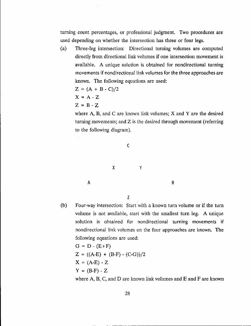
turning count percentages, or professional judgment. Two procedures are
used depending on whether the intersection has three or four legs.
(a) Three-leg intersection: Directional turning volumes are computed
directly from directional link volumes if one intersection movement is
available. A unique solution is obtained for nondirectional turning
movements if nondirectionallink volumes for the three approaches are
known. The following equations are used:
Z = (A + B - C) /2
X = A-Z
Z = B - Z
where A, B, and C are known link volumes; X and Yare the desired
turning movements; and Z is the desired through movement (referring
to the following diagram).
c
x y
A B
Z
(b) Four-way intersection: Start with a known turn volume or if the turn
volume is not available, start with the smallest turn leg. A unique
solution is obtained for nondirectional turning movements if
nondirectional link volumes on the four approaches are known. The
following equations are used:
G = D - (E+F)
Z = ((A-E) + (B-F) - (C-G»/2
X = (A-E) - Z
Y = (B-F) - Z
where A, B, C, and D are known link volumes and E and F are known
28
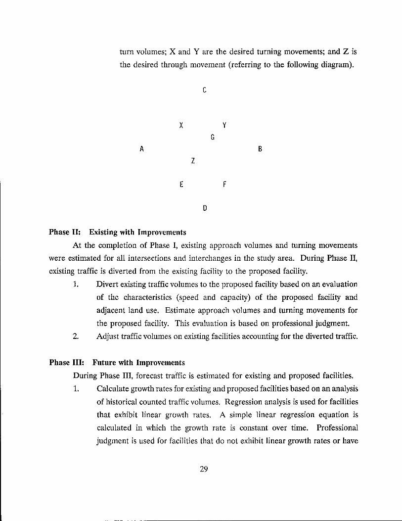
turn volumes; X and Yare the desired turning movements; and Z is
the desired through movement (referring to the following diagram).
c
x y
G
A B
z
E F
o
Phase II: Existing with Improvements
At the completion of Phase I, existing approach volumes and turning movements
were estimated for all intersections and interchanges in the study area. During Phase II,
existing traffic is diverted from the existing facility to the proposed facility.
1. Divert existing traffic volumes to the proposed facility based on an evaluation
of the characteristics (speed and capacity) of the proposed facility and
adjacent land use. Estimate approach volumes and turning movements for
the proposed facility. This evaluation is based on professional judgment.
2. Adjust traffic volumes on existing facilities accounting for the diverted traffic.
Phase III: Future with Improvements
During Phase III, forecast traffic is estimated for existing and proposed facilities.
1. Calculate growth rates for existing and proposed facilities based on an analysis
of historical counted traffic volumes. Regression analysis is used for facilities
that exhibit linear growth rates. A simple linear regression equation is
calculated in which the growth rate is constant over time. Professional
judgment is used for facilities that do not exhibit linear growth rates or have
29
- --------------------------------------------
significant changes in adjacent land use. The following sources of information
are used to establish an appropriate growth rate:
(a) Old traffic maps and historical data.
(b) Old project files.
( c) Historical and forecast adjacent land use.
(d)
(e)
Growth rates for similar existing facilities within the same urban area.
In general, lower growth rates are applied in completely developed
areas; intermediate growth rates are applied in partially developed
areas; and high growth rates are applied to undeveloped areas that are
forecast to develop. The RI Log is used for reference.
2. Calculate future approach and turning movement volumes for the existing and
proposed facilities by applying the appropriate growth rates to the traffic
volumes estimated during Phase II.
Phase IV: Future with Model Assignment
During Phase IV, the forecast traffic assignment produced from the Texas Travel
Demand Package are refined and posted to a detailed schematic.
1. Obtain and post on a straight line network map the future year approach and
turning movement volumes produced by the Texas Large Network Assignment
Models. Normally, these volumes are the result of a weighted capacity
restraint assignment.
Network coding practices used by D-IOP vary by study area. For most urban
areas, the networks are coded as two-way links with a single node representing
an intersection or interchange. For these urban areas, the practice is to post
the approach and turn volumes directly on the network map. For some urban
areas, the freeways are detail coded. This means that the freeway main lanes
are coded as two one-way links, ramps are coded as one-way links, and an
interchange is coded using several nodes rather than as a single node. It is
the practice of the Corridor Analysis Section to first collapse a detail coded
network to a straight line network and collapse the approach and turning
movement volumes as well prior to refining the traffic.
30
2. Revise the straight line network to match the schematic for the proposed
facility. Schematic diagrams for proposed facilities are provided by the
applicable District Office or D-S.
Rarely does a detailed coded network match the schematic for a proposed
facility. There are several reasons for this. The forecast year network is
prepared months or even years before a detailed schematic is prepared. The
schematic for a project will change several times during development of a
project. And finally, the detail coded network for a proposed facility is almost
never to the same degree of detail as the schematic used for project design.
3. Manually reassign the approach and turning movement volumes to the revised
straight line network. Professional judgment is exercised at this stage for two
reasons. The revised straight line network will, of course, not match the
assigned network. The turning movement volumes obtained from a traffic
assignment are subject to error.
Phase V: Final Phase
During Phase V, the straight line approach and turning movement volumes obtained
from Phase III and Phase IV are compared, a decision made on the preferred forecast, and
final volume refinements made to the schematic.
1. Compare the straight line approach and turning movement volumes developed
in Phase III with those developed in Phase IV.
Several factors are considered as part of this comparison. Frequently, the
project year and 20-year forecast will be different than the years for which
traffic assignments are available. Therefore, some interpolation of forecast
volumes will almost always be necessary. The traffic assignment provides an
excellent "pattern" of major traffic movements through a corridor or proposed
project. The traffic assignment may have significant errors for specific turning
movement volumes. The traffic assignment may be based on a different land
use forecast than the land-use forecast available at the time the corridor
analysis is undertaken. This can be particularly significant if the location of
a major traffic generator is known at the time of the corridor analysis, but
31
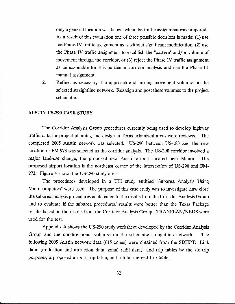
only a general location was known when the traffic assignment was prepared.
As a result of this evaluation one of three possible decisions is made: (1) use
the Phase IV traffic assignment as is without significant modification, (2) use
the Phase IV traffic assignment to establish the "pattern' and/or volume of
movement through the corridor, or (3) reject the Phase IV traffic assignment
as unreasonable for this particular corridor analysis and use the Phase III
manual assignment.
2. Refine, as necessary, the approach and turning movement volumes on the
selected straightline network. Reassign and post these volumes to the project
schematic.
AUSTIN US-290 CASE STUDY
The Corridor Analysis Group procedures currently being used to develop highway
traffic data for project planning and design in Texas urbanized areas were reviewed. The
completed 2005 Austin network was selected. US-290 between US-183 and the new
location of FM-973 was selected as the corridor analysis. The US-290 corridor involved a
major land-use change, the proposed new Austin airport located near Manor. The
proposed airport location is the northeast corner of the intersection of US-290 and FM-
973. Figure 4 shows the US-290 study area.
The procedures developed in a TTl study entitled "Subarea Analysis Using
Microcomputers" were used. The purpose of this case study was to investigate how close
the subarea analysis procedures could come to the results from the Corridor Analysis Group
and to evaluate if the subarea procedures' results were better than the Texas Package
results based on the results from the Corridor Analysis Group. TRANPLAN /NEDS were
used for the test.
Appendix A shows the US-290 study worksheet developed by the Corridor Analysis
Group and the nondirectional volumes on the schematic straightline network. The
following 2005 Austin network data (615 zones) were obtained from the SDHPT: Link
data; production and attraction data; zonal radii data; and trip tables by the six trip
purposes, a proposed airport trip table, and a total merged trip table.
32
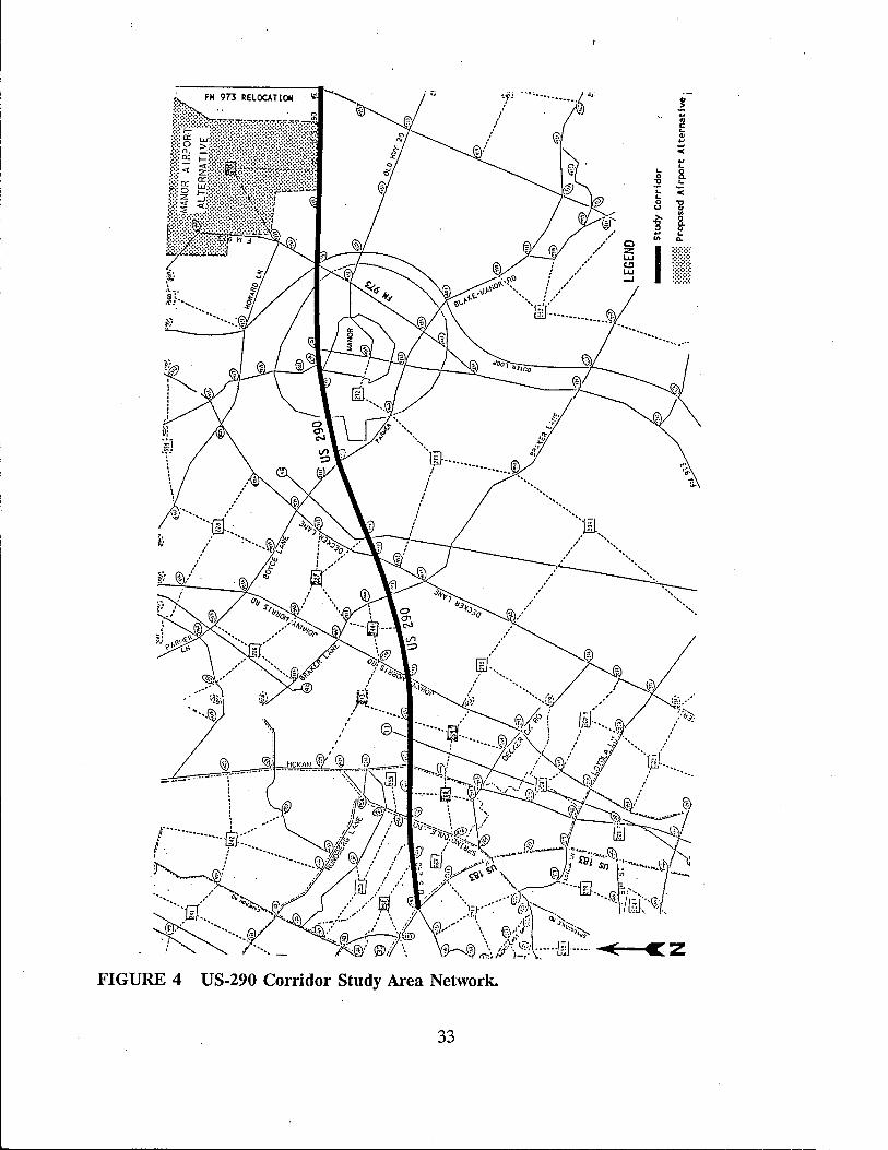
FH 973 RELOCATION
FIGURE 4 US-290 Corridor Study Area Network.
33
~ ~ ., ... c ...
'- 8. :2 ~ '- c
8 ] ~ ~ ... 'II> Q.
1IlIIIIIIIl
LtII( c:z
The 2005 Austin network and trip tables were downloaded to the microcomputer.
The downloaded data were converted from the Texas Model format to TRANPLAN based
on the following procedures:
1. Mount labeled tapes and allocate data sets on disk.
2. Copy from the tape data set to the allocated disk.
3. Convert binary record trip table to 12I6 format using the CVTRP program.
4. Download main frame to microcomputer.
5. Convert trip tables and link data from the Texas Model to TRANPLAN.
Use of Entire Study Area
The subarea assignment technique is primarily applicable to large urban areas.
TRANPLAN capacities are sufficient to handle the entire Austin network. The subarea
analysis procedures can be used in smaller urban areas without any recoding of the study
area.
Every effort was made to obtain assigned volumes as close as possible to the volumes
calculated by the Corridor Analysis Group. The traffic assignment programs in
TRANPLAN were run using the following procedures:
1. Checked the downloaded (and converted to TRANPLAN) Austin trip tables
using the selected zone parameter of the TRANPLAN Report Matrix
function.
2. Ran the TRANPLAN Matrix Manipulate function to merge six trip tables
(home-based-work, home-based-nonwork, nonhome-based, external-local,
external-external, and truck-taxi trip purposes) into one total trip table.
3. Converted the total production and attraction (P / A) trip table to an origin
and destination (O/D) trip table.
4. Ran the TRANPLAN Report Matrix function to be sure that the OlD trip
table was converted correctly.
5. Converted the link data of the Texas Model to the TRANPLAN format using
the link data conversion program developed by TIL
6. Built the Austin highway network (2005) using the Build Highway Network
34
function in TRANPLAN.
7. Ran the traffic assignment using the five different techniques (all-or-nothing,
stochastic, iterative, incremental and equilibrium assignments). The following
parameters and options were used:
Assign Techniques Parameters and Options
All-or-nothing Save Turn
Stochastic Theta = 0.02
Iterative
Incremental
Iteration = 5 and Save Turn
15, 15,20,20,30% and Save Turn
Equilibrium Iteration = 5 and Save Turn
The following nodes were selected along the study corridor (US-290 between
US-183 and FM-973) for the turning movements using the following
parameter specification:
SAVE TURNS = 1169, 1170, 1990, 1995, 2038, 2040-2043, 2045,
2049, 2061, 2062, 2065, 3837-3842
8. The Report Highway Load function was used to report assigned volumes from
all five traffic assignment techniques. Turn volumes and selected link volumes
on US-290 were obtained by using the following options:
Minimum Report: Any link with zero volume will not be reported.
Print Turns: All nodes for which turn volumes were saved
during loading are to be reported.
Suppress Links:
Turns File:
VC Report:
Only turn volumes are to be reported.
Turning movements are written to the TRNDATA
file in ASCII format.
One-way V / C calculations are reported for all
links selected, as well as the respective volumes
and capacities.
Table 2 shows the through and turn volumes along US-290 and the percent
differences between the Corridor Analysis Group results and the TRANPLAN results.
The multipath stochastic assignment does not have an option for the turning movement (no
Save Turn option). The stochastic assignment produced assigned link volumes similar to
35
the all-or-nothing assignment.
The schematic map was used for posting the turn and assigned volumes for each
intersection. Appendix B shows the three different sources of the intersection volumes
(from the Corridor Analysis Group, the Texas Package, and TRANPLAN) posted on three
intersections along US-290. There was a significant difference between the manual
calculation results from the Corridor Analysis Group and the results from TRANPLAN.
The results from the Texas Package were compared with TRANPLAN because there
is a very significant difference between the manual calculation results of the Corridor
Analysis Group and the TRANPLAN results. The TRANPLAN assigned link volumes were
compared with the Texas Package volumes. The assigned (resulted) volumes from both
packages using the all-or-nothing and capacity restraint assignment techniques were similar.
The volume constraint assignments were tested by replacing the coded link capacities with
the link volumes calculated by the Corridor Analysis Group. The volume constraint
assignment results were not any better than the capacity restraint assignment results (see
Table 2). This may be because there is no highway parallel to US-290.
Turning movement estimates for the intersection of US-290 and US-183 were studied
(see Figure 5). The Corridor Analysis Group turning movement volumes as a proportion
of through movements appeared high. For some reason which was not determined, the
Corridor Analysis Group increased the number of trips going to or from Zone 254. On the
original network, Zone 254 connected to three nodes and produced a total of 19,379 trip
ends. On the network as revised by the Corridor Analysis Group, the link volume on the
centroid connector to US-290, (the link from Node 254 to Node 1169) was 28,400 trips. A
high percentage of these additional trips made a turn at the intersection of US-290 and US-
183.
36
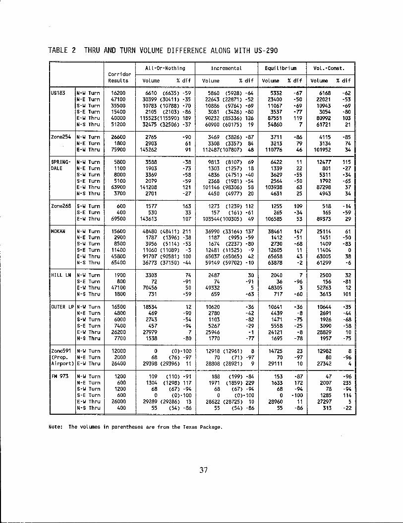
TABLE 2 THRU AND TURN VOLUME DIFFERENCE ALONG WITH US-290
~ I All-Or-Nothing Incremental Equilibrium Vol.-Const.
~ Corridor Results Volume % dif Volume % dif Volume % dif Volume % dif
~US183 N-W Turn 16200 I 6610 (6635) -59 5860 (5928) -64 5332 -67 6168 -62 ~ N-E Turn 47100 30399 (30411) -35 22643 (22871) -52 23400 -50 22021 -53
i S-W Turn 35500 10783 (10788) -70 10886 (9764) -69 11067 -69 10943 -69 S-E Turn 15400 2105 (2103) -86 3081 (3426) -80 3537 -77 3054 -80
I E-W Thru 40000 115523(115590) 189 90232 (85336) 126 87551 119 80992 103 N-S Thru 51200 32475 (32506) -37 60900 (60175) 19 54860 7 61721 21
Zone254 N-W Turn 26600 2765 -90 3469 (3826) -87 3711 -86 4115 -85 N-E Turn 1800 2903 61 3308 (3357) 84 3213 79 3134 74 E-W Thru 75900 145262 91 112487(107807) 48 110776 46 101952 34
SPRING- N-W Turn 5800 3588 -38 9813 (8107) 69 6422 11 12477 115 DALE IN-E Turn 1100 1903 -73 I 1303 ( 1257) 18 1339 22 801 -27
I IS-W Turn 8000 I 3369 -58 I 4836 (4751) -40 3629 -55 5311 -34 S-E Turn 5100 2079 -59
I 2368 (1981 ) -54 2564 -50 1792 -65
E-W Thru 63900 141208 121 101146 (98306) 58 103938 63 87298 37
"
N-S Thru I 3700 2701 -27 I 4450 (4977) 20 I 4631 25 4943 34 I
~zone268 IS-W Turn I
600 1577 163 I
1273 (1239) 112 1255 109 I
518 -14 i S-E Turn 400 530 33 157 (161) -61 265 -34 165 -59
~ IE-W Thru 69500 143613 107 I 103544(100305) 49 106585 53 I 89373 29 ~ ii i
I II MOKAN IN-W Turn 15600 48480 (48411) 211 36990 (33164) 137 38461 147 25114
61 I N-E Turn 2900 1787 (1396) -38 1187 (995) -59 1412 -51 1451 -50 II IS-w Turn I 8500 3956 (5114) -53 1674 (2237) -80 2730 -68 1409 -83 ~ IS-E Turn
I 11400 11060 (11089) -3 12481 (11525) -9 12605 11
I 11404 o I
~ E-W Thru 45800 91707 (90581) 100 65037 (65065) 42 65658 43 63005 38 I N-S Thru 65400 36773 (37150) -44 59149 (59702) -10 63878 -2 61299 -6
IHILL LN N-W Turn 1900 3303 74 2487 30 2040 7 2500 32
I S-E Turn 800 72 -91 74 -91
I 36 -96 156 -81
E-W Thru 47100 70456 50 49332 5 48305 3 52763 12 N-S Thru 1800 731 -59 659 -63 717 -60 3613 101
I!0UTER LP N-W Turn I
16500 18534 12 10620 -36 10641 -36 10644 -35 N-E Turn 4800 469 -90 2780 -42 4439 -8 2691 -44
IS-W Turn I 6000 2743 -54 1103 -82 1471 -75 1926 -68 I S-E Turn 7400 457 -94 5267 -29 5558 -25 3090 -58 I
IE-W Thru 26200 27979 7 25946 -1 24121 -8 28829 10 ! N-S Thru 7700 1538 -80 1770 -77 1695 -78 1957 -75 ii
Zone591 IN-W Turn 12000 0 (0)-100 I 12918 (12961) 8 14725 23 12982 8 I I (Prop. I N-E Turn 2000 68 (76) -97 70 (71 ) -97 70 -97 I 80 -9~
Airport) E-W Thru 26400 29398 (29396) 11 28808 (28921) 9 29111 10 27342 i i i
IFM 973 N-W Turn 1200 109 (110) -91 I 188 (199) -84 153 -87 I 47 -96 i
! N-E Turn I 600 1304 (1298) 117 1971 (1859) 229 1633 172 I 2007 235 I S-W Turn 1200 68 (67) -94 68 (67) -94 68 -94 78 -94
I S-E Turn 600 o (0)-100 I 0 (0)-100 0 -100 I 1285 11~ I E-W Thru I 26000
I 29289 (29286) 13 28622 (28725) 10 28960 11 27297
N-S Thru 400 55 (54) -86 i 55 (54) -86 55 -86 i 313 -22 i Note: The volumes in parentheses are from the Texas Package.
37
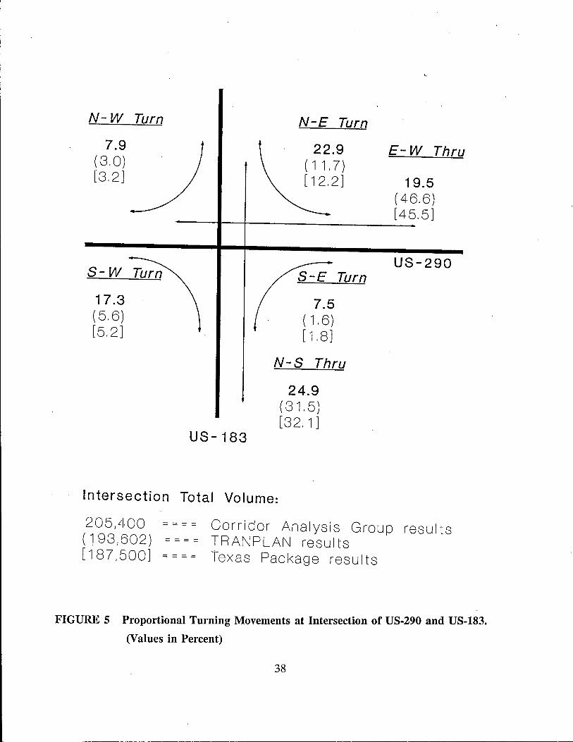
N- W Turn
7.9 (3,0) [3,2]
S-W
17.3 (5,6) [5,2]
N-E Turn
22.9 (11,7) [12,2]
S-E Turn
7.5 ( 1 ,6) [1,8]
N-S Thru
US-183
Intersection Total Volume:
24.9 (31,5) [32,1]
E- W Thru
19.5 (46,6) [45,5]
US-290
205,400 = = = = Corridor Analysis Group resul ts (193,602) ==== TRANPLAN results [187,500] ==== Texas Package results
FIGURE 5 Proportional Turning Movements at Intersection of US-290 and US-1S3.
(Values in Percent)
38
Conclusions of US-290 Case Study
The US-290 case study compared assignments produced using the TRANPLAN
subarea analysis procedures with the Corridor Analysis Group results. It was hoped that
TRANPLAN subarea analysis procedures would produce "better" assignments than the
Texas Package, "better" meaning assigned volumes closer to those developed by the
Corridor Analysis Group. This did not occur. There was a significant difference between
the TRANPLAN and Corridor Analysis Group assigned volumes. The Texas Package
assignments and TRANPLAN subarea analysis assignments were similar. The volume
constraint assignment results were similar to the capacity restraint assignment. None of the
procedures tested were able to match the Corridor Analysis Group results.
39
CHAPTER III. APPLICATION OF ALTERNATIVE PROCEDURE
ALTERNATIVE PROCEDURE
Corridor analysis needs to be performed using standardized and documented
procedures, and, to the extent practical, microcomputer software. This will help assure the
production of the high quality, consistent, and timely forecasts. However, the procedures
must be applied with considerable judgment by a trained analyst. The following alternative
procedures were developed and are recommended for evaluation by the Corridor Analysis
Group.
Phase I: Existing
During Phase I, existing traffic is assigned to existing facilities.
1. Obtain straightline network. The straightline network is a simplification of
the actual highway system that contains the study facility, intersecting arterials,
and a zonal centroid called "area." The need to forecast traffic volumes for
a major facility (highway or freeway) is usually the reason for conducting a
corridor analysis. Each existing or proposed facility is represented by a
straight line. The Corridor Analysis Group calls this straightline network a
"picture."
2. Collect existing traffic volumes. Traffic counts are obtained from a variety
of sources.
(a) Own counts: The traffic counts may be made by the Corridor Analysis
Group or other D-IO staff. Through movements are counted by
automatic count record equipment. Directional turning movement
percentages may be obtained by counting or by direct observation.
Turning movement percentages made by observation require
professional judgment based on experience.
(b) Freeway ramp map, semipermanent record, automatic traffic record,
and/ or automatic count record: Permanent count stations provide
trend data. Average daily traffic estimates and annual average daily
40
traffic estimates are available for locations with semipermanent record
and automatic traffic record equipment. The annual report from the
permanent automatic traffic recorders shows for an estimate of volume
for each location, the directional distribution, the peak-hour factor,
and the K-factor.
The semipermanent record location that is nearest the study area
provides a starting point for estimating freeway volumes in the study
area. The volumes in the study area are estimated by adding or
subtracting counted ramp volumes recorded on the ramp map.
(c) Others: Traffic counts are also obtained from traffic maps, urban
studies, and projects files of previously completed adjacent corridor
analysis studies. Information on new development that will impact
volume estimates is obtained from SDHPT Districts Offices or from
the consulting firm assisting with the project. The RI (road inventory)
LOG is used for reference.
3. Calculate existing turn volumes and adjust approach volumes for each study
area intersection or interchange using counted turn percentage data, observed
turning count percentages, or professional judgment. Two procedures are
used depending on whether the intersection has three or four legs.
(a) Three-leg intersection: Directional turning volumes are computed
directly from directional link volumes if one intersection movement is
available. A unique solution is obtained for nondirectional turning
movements if nondirectionallink volumes for the three approaches are
known. The following equations are used:
Z = (A + B - C)/2
X = A- Z
Z = B - Z
where A, B, and C are known link volumes; X and Yare the desired
turning movements; and Z is the desired thm movement (referring
to the next diagram).
41
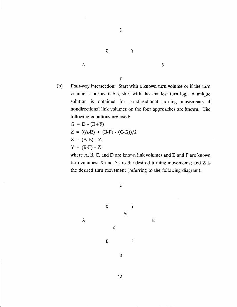
c
x y
A B
Z
(b) Four-way intersection: Start with a known turn volume or if the turn
volume is not available, start with the smallest turn leg. A unique
solution is obtained for nondirectional turning movements if
nondirectional link volumes on the four approaches are known. The
following equations are used:
G = D - (E+F)
Z = ((A-E) + (B-F) - (C-G))/2
X = (A-E) - Z
Y = (B-F) - Z
where A, B, C, and D are known link volumes and E and F are known
turn volumes; X and Yare the desired turning movements; and Z is
the desired thru movement (referring to the following diagram).
c
x y
G
A B
z
E F
o
42
Phase II: Existing with Improvements
At the completion of Phase I, existing approach volumes and turning movements
were estimated for all intersections and interchanges in the study area. During Phase II,
existing traffic is diverted from the existing facility to the proposed facility.
1. Divert existing traffic volumes to the proposed facility based on an evaluation
of the characteristics (speed and capacity) of the proposed facility and
adjacent land use. Estimate approach volumes and turning movements for
the proposed facility. This evaluation is based on professional judgment.
2. Adjust traffic volumes on existing facilities accounting for the diverted traffic.
Phase III: Run Base Year Traffic Assignment Using Subarea Analysis
1. Define the subarea including, if possible, at least two parallel roadways within
the study corridor.
2. Set up a run of the Texas Large Network Assignment Model to assemble the
full study area network, and then run the Subarea Windowing Program.
3. Download the data (Le., link data, zonal productions and attractions, radii
data, fifth relative values, XY coordinates, and trip tables) to microcomputer.
4. Convert the downloaded data from the Texas Package format to TRANPLAN.
5. Revise the future network into the detailed (schematic) network if needed.
6. Run the TRANPLAN traffic assignments.
Phase IV. Validate Model and Run Future Year Assignment Using Subarea Analysis
Phase VI. Refine Future Year Link Volumes Using Factoring Procedures
The computations are to adjust the future year link volumes to account for probable
assignment errors. The underlying assumption used is that errors occurring in a base year
assignment will continue to occur proportionally in any future year assignment. A future
year link volume is adjusted using two methods: (1) the ratio of the adjusted base year
traffic count on the existing network with improvements (results from Phase II) to the
validated base year assignment (results from Phase IV) and (2) the numerical difference
between the adjusted base year traffic count and the validated base year assignment. Then,
a subsequent adjustment is made which is the average of the two methods.
43
1. Input Data and Output:
(a) Future year assigned volume (Fi) from Phase V.
(b) Base year assigned volume (B.i) from Phase IV.
( c) Base year ground counts (Be) from Phase II.
(d) Output: Adjusted future year link volume (Vi).
2. Ratio Method: Vri = Fi x (Be/B.)
3. Difference Method: Vdi = Fi + (BecBa)
4. Combined Method: Vfi = (Vfj+ Vdi)/2
Phase VII. Calculate Future Turning Movements Using Iterative Procedures
The iterative procedures adjust future year turning movements to match as closely
as possible a predetermined estimate of turning percentages. The turning movement
iterative procedures are from NCHRP Report 255, pages 105-108 (1). Iteration involves
applying a technique repeatedly until the results converge to an acceptable result. Iteration
is required to balance the volume of traffic entering and leaving the intersection. Future
year link volumes are fixed using this method and the turning movements are adjusted to
match.
1. Input Data:
(a) Future year directional link volumes from Phase VI.
(b) Initial estimate of future directional turning percentages from Phase
II.
2. Iterative Procedures:
(a)
(b)
(c)
(d)
(e)
(f)
Step 1:
Step 2:
Step 3:
Step 4:
Step 5:
Step 6:
Construct initial turning movement matrix.
Perform the first row iteration.
Perform the first column iteration.
Repeat row iteration.
Repeat column iteration.
Continue the iterations until acceptable values are
obtained.
Note: The final adjusted directional turning and thru movements should be reviewed
for reasonableness.
44
SH-161 CASE STUDY IN DALLAS-FORT WORTH
The SH-161 project was selected for evaluation of the proposed alternative
procedures. Only part of the alternative procedures were able to be evaluated because the
base year data was not available. The alternative procedure results were compared to the
Corridor Analysis Group results. The proposed SH-161 from IH-20 to IH-635 in the D
FW area (see Figure 6) was chosen because the project, including the forecast average
daily traffic volumes and turning movements, had already been completed by the Corridor
Analysis Group.
The purpose of this case study was to test the alternative procedures. The
alternative procedures are intended to reduce the manual work required by substituting
travel demand modeling software for a part of the manual labor. The proposed SH-161
runs through Irving and Grand Prairie, connects with IH -635 on the north, intersects IH-
30 in the middle, and connects with IH-20 on the south. The year 2010 D-FW total trip
table and the future network with improvements were provided by the SDHPT Regional
Planning Office in Arlington. A series of network plots associated with the improvements
were provided as well.
Subarea Window Procedure
The microcomputer packages have different network design limits. The network size
limits also vary according to the amount of main memory available. TRANPLAN is
designed for 3,000 zones and 32,000 links; however, 1,500 zones, 8,000 nodes, and 9,000
links can be processed on a 640 Kbytes-RAM microcomputer. The subarea assignment
technique is primarily applicable to studies in large areas such as San Antonio, Houston
Galveston, and Dallas-Fort Worth.
TTl Research Report 1110-4F (22) provides a detailed description of subarea
analysis procedures. A major application of subarea analysis is the study of proposed future
land-use and transportation alternatives. A subarea assignment technique is applicable to
alternatives involving major changes to the transportation system, major land-use changes,
or both. The proposed SH-161 project is a major change to the transportation system.
45
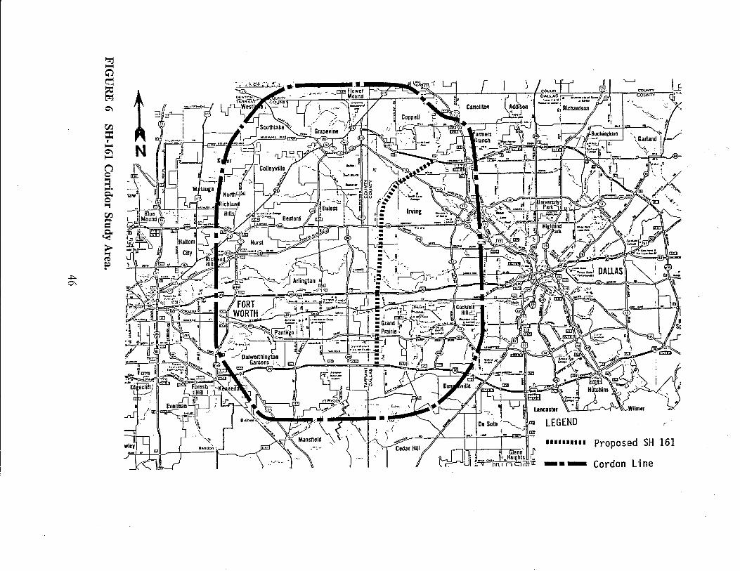
~ -Ci
~
1 Q\
r:n == • ~ Q\ ~
(i 0 '"l '"l ..... !:lo 0 '"l
r:n .... = !:lo '<
~ (t)
F +>-0\
.......... Proposed SH 161
--- Cordon Line
One of the subarea assignment approaches, the subarea window approach, was used
in this case study. Using this approach, the subarea was identified and only those zones and
the network within the subarea were carried forward in the subarea analysis procedure. In
essence, the network and zones within the subarea were isolated and treated as a small
stand-alone study area. Traffic entering or leaving the subarea was treated as external
traffic relative to the subarea. The subarea's external traffic is predominantly composed
of internal traffic relative to the larger study area.
Use of Subarea Window Technique in Texas Package
1. Chose the approximate area of the subarea along SH-161. The subarea was
a substantially larger area than the subarea of interest. The window area
covered West Loop 12 in Dallas and East Loop IH-820 in Fort Worth.
2. Drew a cordon line on the map which surrounds the subarea. The following
rules were used:
(a) The subarea cordon line should not pass through any nodes or
centroids.
(b) When the cordon line intersected a centroid connector, the associated
centroids were inside the cordon line. Each node immediately outside
the cordon became an external station for the subarea. A centroid
should not function as an external station.
(c) The cordon line should not intersect (1) a zonal centroid connector
which had only one centroid connector or (2) all the centroid
connectors that a zonal centroid had because the internal trips from
or to that zone were isolated.
(d) The windowed subarea should be completely closed without any
missing external station link.
3. Checked the cordon line to insure that it completely surrounded the subarea
and that it followed the rules above. The Path Trace function in the Texas
Package was employed to check if there were any missing links.
4. Chose a link intersected by the cordon line and recorded all links and
47
connectors crossed by the cordon line. Each link, called an External Station
Link, was entered on an External Station Link card image.
5. Picked a centroid inside the cordon line and entered the centroid number on
the Direction Card image. Centroid 973 was chosen as the zone inside the
cordon line.
6. Set up a run of the Texas Large Network Assignment Models to assemble the
full study area network and then ran the Subarea Windowing program. This
program renumbered the centroids within the subarea starting at "1." Then
the nodes which constitute the external stations were renumbered.
7. Examined the run. There were errors in the external station links. The errors
were corrected and the program was rerun.
8. Ran trip matrix collapse and saved the resulting windowed trip matrix.
Downloading Procedure
The conversion (Le., downloading and/or uploading) program which is a part of the
subarea analysis was used. Two output data sets from the subarea window program, total
trip table and link data, were generated and downloaded from the Texas Package to
TRANPLAN. Node numbers larger than 9,999 had to be renumbered because
TRANPLAN can handle a maximum of 9,999 nodes. The renumbered node numbers were
inserted into gaps between Node 1 and Node 9,999.
The downloaded/windowed network consisted of 444 internal zones, 118 external
stations, 1,098 internal centroid connectors, and 4,764 nondirectional (two-way) links. The
windowed network was revised into the detailed schematic network. Forty new links were
added along SH-161. The Build Highway Network program in TRANPLAN was run.
Use of Traffic Assignment
The incremental assignment in TRANPLAN was run. In order to get the turning
movement result from the TRANPLAN traffic assignment, the following steps were needed:
1. Select a series of interchanges on SH-161 (usually three to six interchanges
48
with less than 50 nodes because TRANPLAN can save turn volumes up to 50
nodes during one loading).
2. Recode all node numbers inside the selected interchanges.
3. Run TRANPLAN with the parameter specification as SA VB TURNS = list
of nodes.
The study area was divided into three portions: south, central, and north. Three
interchanges were selected in each portion for the turning movement comparisons. The
comparisons of the TRANPLAN results with the Corridor Analysis Group Results are
shown in Table 3 (south portion), Table 4 (central portion), and Table 5 (north portion).
Turning movement volumes from the Texas Travel Demand Model using the entire D-FW
_ network are also included in Tables 3, 4, and 5. Appendix C shows an example of the
turning movements for one intersection. There was a significant difference between the
results of the Corridor Analysis Group and TRANPLAN. The comparison between the
Texas Travel Demand Model and TRANPLAN using the subarea window assignment
technique resulted in similar thru and turning movement volumes.
Like most modeling packages, TRANPLAN assigned "zero" turning and thru volumes
at some intersections (see Figure 7). The locations with "zero" assigned volumes were
investigated and identified:
1. V-turn underpass of freeway: No zonal centroids near the frontage road. In
TRANPLAN, drivers are assumed to be 100 percent rational and make no
mistakes in choosing their routes. However, in reality, the V-turn underpass
of a freeway is frequently used by drivers who miss their intended exit and
need to return to some upstream locations.
2. Thru movement on frontage road: No zonal centroids near the frontage
road.
3. Turn movements from or to frontage road: No zonal centroids toward the
turning direction. Alternative routes are available that take shorter travel
time.
In summary, two reasons explain most of these "zero" assigned volumes: (1) A
centroid is an assumed point in a zone that represents the origin or destination of all trips
to or from the zone and (2) the path algorithm is based on the minimum path.
49
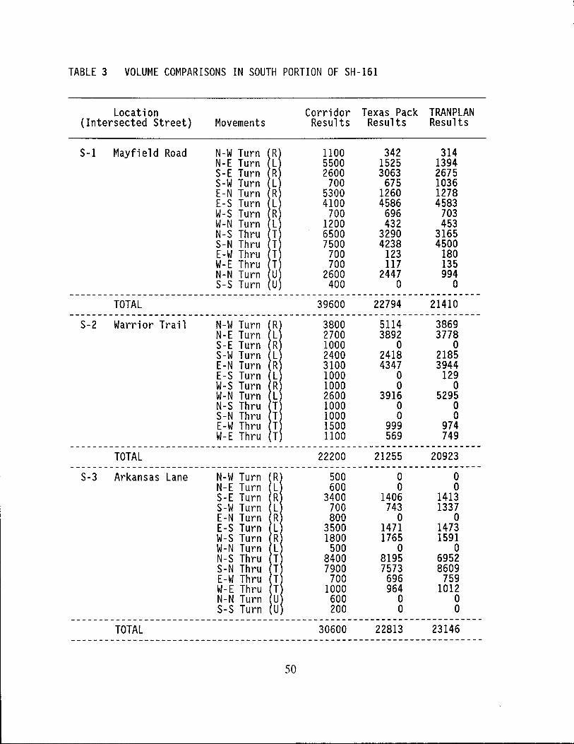
TABLE 3 VOLUME COMPARISONS IN SOUTH PORTION OF SH-161
Location Corridor Texas Pack TRANPLAN (Intersected Street) Movements Results Results Results
S-l Mayfi e 1 d Road N-W Turn R 1100 342 314 N-E Turn L 5500 1525 1394 S-E Turn R 2600 3063 2675 S-W Turn L 700 675 1036 E-N Turn R 5300 1260 1278 E-S Turn L 4100 4586 4583 W-S Turn R 700 696 703 W-N Turn L 1200 432 453 N-S Thru T 6500 3290 3165 S-N Thru T 7500 4238 4500 E-W Thru T 700 123 180 W-E Thru T 700 117 135 N-N Turn U 2600 2447 994 S-S Turn U 400 0 0
-------------------------------------------------------------------------TOTAL 39600 22794 21410
-------------------------------------------------------------------------S-2 Warrior Trail N-W Turn R 3800 5114 3869
N-E Turn L 2700 3892 3778 S-E Turn R 1000 0 0 S-W Turn L 2400 2418 2185 E-N Turn R 3100 4347 3944 E-S Turn L 1000 0 129 W-S Turn R 1000 0 0 W-N Turn L 2600 3916 5295 N-S Thru T 1000 0 0 S-N Thru T 1000 0 0 E-W Thru T 1500 999 974 W-E Thru T 1100 569 749
-------------------------------------------------------------------------TOTAL 22200 21255 20923
-------------------------------------------------------------------------S-3 Arkansas Lane N-W Turn R 500 0 0
N-E Turn L 600 0 0 S-E Turn R 3400 1406 1413 S-W Turn L 700 743 1337 E-N Turn R 800 0 0 E-S Turn L 3500 1471 1473 W-S Turn R 1800 1765 1591 W-N Turn L 500 0 0 N-S Thru T 8400 8195 6952 S-N Thru T 7900 7573 8609 E-W Thru T 700 696 759 W-E Thru T 1000 964 1012 N-N Turn U 600 0 0 S-S Turn U 200 0 0
-------------------------------------------------------------------------TOTAL 30600 22813 23146
-------------------------------------------------------------------------
50
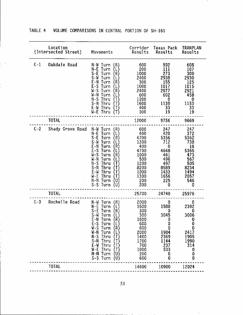
TABLE 4 VOLUME COMPARISONS IN CENTRAL PORTION OF SH-161
Location Corridor Texas Pack TRANPLAN (Intersected Street) Movements Results Results Results
C-1 Oakdale Road N-W Turn R 600 592 608 N-E Turn L 200 111 107 S-E Turn R 1000 273 300 S-W Turn L 2400 2938 2930 E-N Turn R 300 155 125 E-S Turn L 1000 1017 1015 W-S Turn R 2400 2877 2921 W-N Turn L 600 602 458 N-S Thru T 1200 0 0 S-N Thru T 1600 1139 1153 E-W Thru T 400 33 33 W-E Thru T 300 19 19
-------------------------------------------------------------------------TOTAL 12000 9756 9669
-------------------------------------------------------------------------C-2 Shady Grove Road N-W Turn R 600 247 247
N-E Turn L 400 420 372 S-E Turn R 4700 5356 5362 S-W Turn L 1300 712 738 E-N Turn R 400 0 16 E-S Turn L 4700 4648 5365 W-S Turn R 1000 461 473 W-N Turn L 500 496 567 N-S Thru T 1200 497 505 S-N Thru T 8200 8589 8234 E-W Thru T 1000 1433 1494 W-E Thru T 1300 1656 2057 N-N Turn U 200 225 546 S-S Turn U 200 0 0
-------------------------------------------------------------------------TOTAL 25700 24740 25976
-------------------------------------------------------------------------C-3 Rochelle Road N-W Turn R 2000 0 0
N-E Turn L 1600 1588 2392 S-E Turn R 300 0 0 S-W Turn L 300 3045 3006 E-N Turn R 1600 0 0 E-S Turn L 600 0 0 W-S Turn R 600 0 0 W-N Turn L 2000 1984 2417 N-S Thru T 1400 2369 1905 S-N Thru T 1700 1144 1990 E-W Thru T 700 237 314 W-E Thru T 1000 533 0 N-N Turn U 200 0 0 S-S Turn U 600 0 0
-------------------------------------------------------------------------TOTAL 14600 10900 12024
-------------------------------------------------------------------------
51
'---------------------------------------
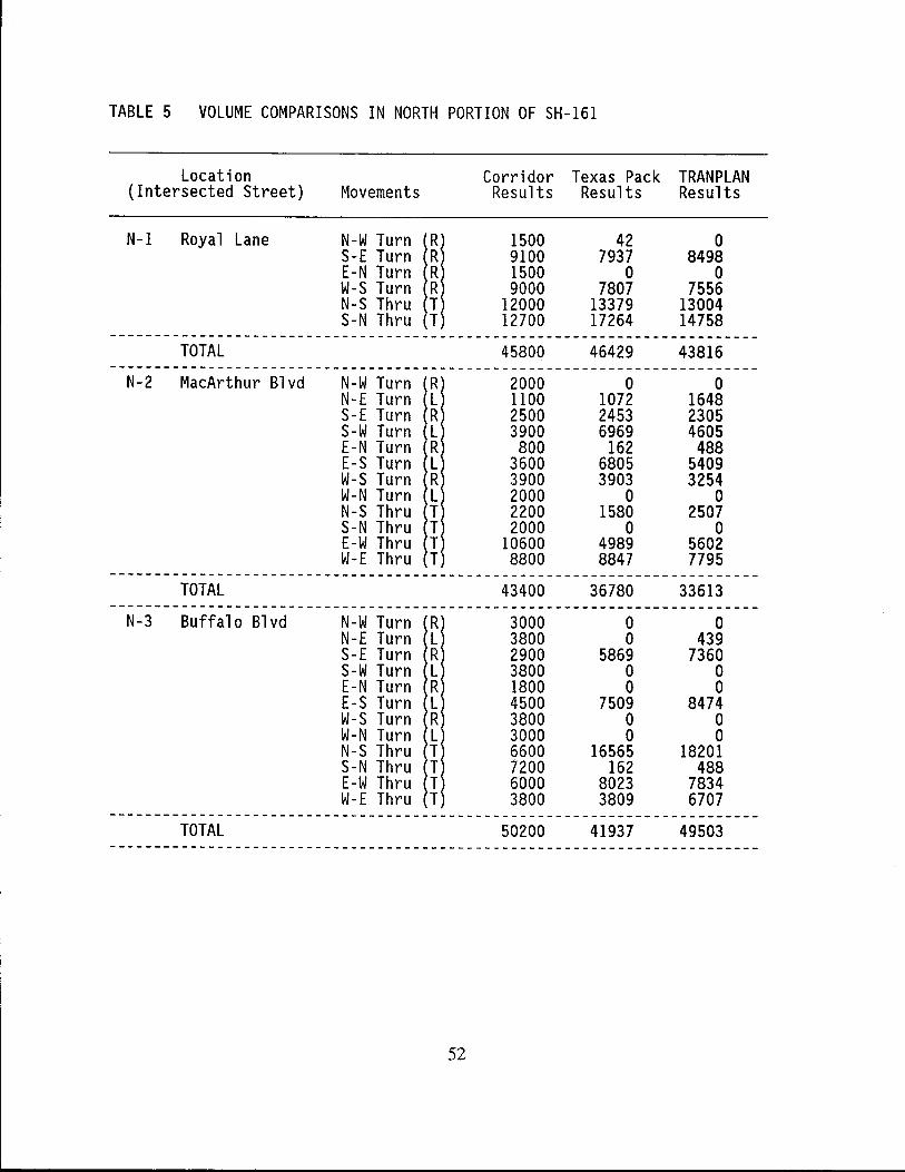
TABLE 5 VOLUME COMPARISONS IN NORTH PORTION OF SH-161
Location Corridor Texas Pack TRANPLAN (Intersected Street) Movements Results Results Results
N-1 Royal Lane N-W Turn R 1500 42 0 S-E Turn R 9100 7937 8498 E-N Turn R 1500 0 0 W-S Turn R 9000 7807 7556 N-S Thru T 12000 13379 13004 S-N Thru T 12700 17264 14758
-------------------------------------------------------------------------TOTAL 45800 46429 43816
-------------------------------------------------------------------------N-2 MacArthur Blvd N-W Turn R 2000 0 0
N-E Turn L 1100 1072 1648 S-E Turn R 2500 2453 2305 S-W Turn L 3900 6969 4605 E-N Turn R 800 162 488 E-S Turn L 3600 6805 5409 W-$ Turn R 3900 3903 3254 W-N Turn L 2000 0 0 N-$ Thru T 2200 1580 2507 $-N Thru T 2000 0 0 E-W Thru T 10600 4989 5602 W-E Thru T 8800 8847 7795
-------------------------------------------------------------------------TOTAL 43400 36780 33613
-------------------------------------------------------------------------N-3 Buffalo Blvd N-W Turn R 3000 0 0
N-E Turn L 3800 0 439 S-E Turn R 2900 5869 7360 S-W Turn L 3800 0 0 E-N Turn R 1800 0 0 E-$ Turn L 4500 7509 8474 W-$ Turn R 3800 0 0 W-N Turn L 3000 0 0 N-$ Thru T 6600 16565 18201 $-N Thru T 7200 162 488 E-W Thru T 6000 8023 7834 W-E Thru T 3800 3809 6707
-------------------------------------------------------------------------TOTAL 50200 41937 49503
-------------------------------------------------------------------------
52
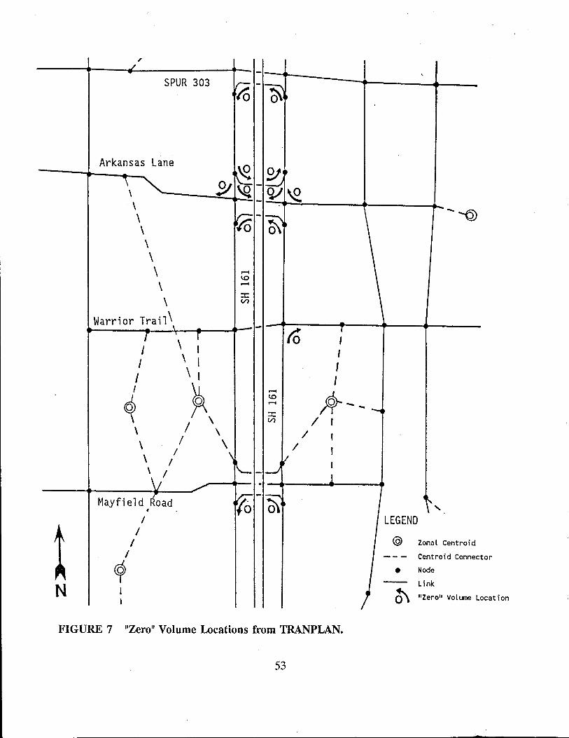
, J
"
SPUR 303 ?o 11\
Arkansas Lane ~ "\ $I I\Q \
\ \ IPo \
£I ~ ~ ~ .-::--'\ -'Q) O\~
\ \ \ ,....,
lO
\ ,...., ::r:
\ V')
Warrior Trail\ -T \
r J I I \ I
I \ I I
~ ~ / \\ \ \ I \ \ / \
'--\ I
\i
-to I , ,
I I
.....
Ar-- -lO ,...., ::r: V') I I
/ I / r
I--"V I
1 -Mayfield Road r;; •
I-=--", 0\. l', \
/
1 I
I I
~ N I
I
LEGEND
@ Zonal Centroid
--- Centroid Connec
• Node
-- Link
b\ "Zero" Voll.l1le L
tor
ocation
FIGURE 7 "Zero" Volume Locations from TRANPLAN.
53
Use of Turning Movement Iterative Procedure
The turning movement iterative procedure, a part of the alternative procedure, was
performed using a combination of the TRANPLAN assignment results and Corridor
Analysis Group results. The turning movement iterative procedures were from NCHRP
Report 255. The Lotus program developed by FHWA and modified by COMSIS was used
for calibrating the turning movements. Appendix D shows the input and output files from
the Lotus program.
Three interchanges (Arkansas Lane, Shady Grove Road, and MacArthur Boulevard)
along SH-161 were selected for the turning movement comparisons. The row and column
iterations were continued until a difference of less than 10% was obtained. The differences
in row totals for all three interchanges were within 10% after the second iteration. The
base year traffic data were not available in this study. The following computational
procedures were used:
Step 1: Construct an initial future year turning movement using estimated turn
percentages that are derived from the Corridor Analysis Group volume
forecast.
Step 2:
Step 3:
Step 4:
Use TRANPLAN assigned link inflow and outflow volumes as the row
and the column totals, respectively.
Perform the first row iteration.
Perform the first column iteration.
Step 5: Repeat row iteration.
Step 6: Repeat column iteration.
Table 6 shows the results of the turning movements from the three results (Corridor
Analysis Group, TRANPLAN, and iterative procedures). The iterative procedures
produced closer results to those results produced by the Corridor Analysis Group than the
TRANPLAN results.
Conclusions of SH·161 Case Study
The alternative procedure was evaluated in comparison with the Corridor Analysis
Group results. The turning movement differences between the iterative procedures and the
54
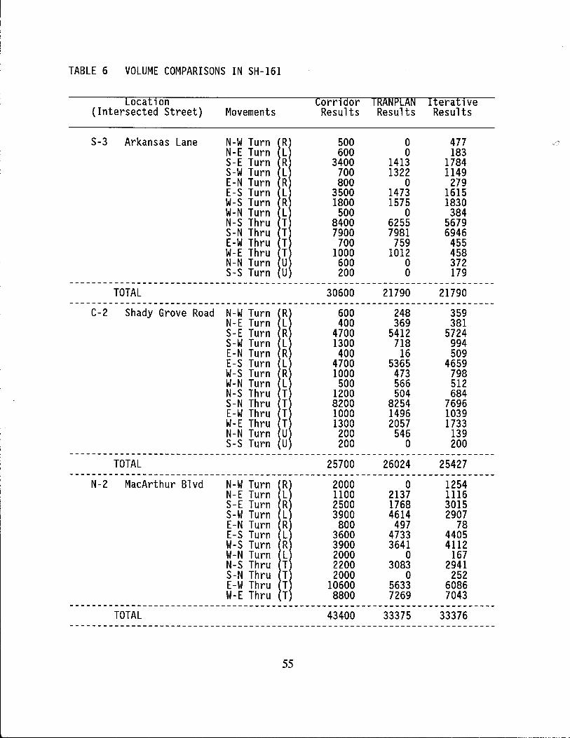
TABLE 6 VOLUME COMPARISONS IN SH-161
Location Corridor 1 RANPLAN Iterative (Intersected Street) Movements Results Results Results
S-3 Arkansas Lane N-W Turn R 500 0 477 ~
N-E Turn L 600 0 183 S-E Turn R 3400 1413 1784 S-W Turn L 700 1322 1149 E-N Turn R 800 0 279 E-S Turn L 3500 1473 1615 W-S Turn R 1800 1575 1830 W-N Turn L 500 0 384 N-S Thru T 8400 6255 5679 S-N Thru T 7900 7981 6946 E-W Thru T 700 759 455 W-E Thru T 1000 1012 458 N-N Turn U 600 0 372 S-S Turn U 200 0 179
----------------------------------------------------------------------------TOTAL 30600 21790 21790
----------------------------------------------------------------------------C-2 Shady Grove Road N-W Turn R 600 248 359
N-E Turn L 400 369 381 S-E Turn R 4700 5412 5724 S-W Turn L 1300 718 994 E-N Turn R 400 16 509 E-S Turn L 4700 5365 4659 W-S Turn R 1000 473 798 W-N Turn L 500 566 512 N-S Thru T 1200 504 684 S-N Thru T 8200 8254 7696 E-W Thru T 1000 1496 1039 W-E Thru T 1300 2057 1733 N-N Turn U 200 546 139 S-S Turn U 200 0 200
----------------------------------------------------------------------------TOTAL 25700 26024 25427
----------------------------------------------------------------------------N-2 MacArthur Blvd N-W Turn R 2000 0 1254
N-E Turn L 1100 2137 1116 S-E Turn R 2500 1768 3015 S-W Turn L 3900 4614 2907 E-N Turn R 800 497 78 E-S Turn L 3600 4733 4405 W-S Turn R 3900 3641 4112 W-N Turn L 2000 0 167 N-S Thru T 2200 3083 2941 S-N Thru T 2000 0 252 E-W Thru T 10600 5633 6086 W-E Thru T 8800 7269 7043
----------------------------------------------------------------------------TOTAL 43400 33375 33376
----------------------------------------------------------------------------
55
Corridor Analysis Group were less than an average of 30%. The turning movement
iterative procedure eliminated the problem "zero" directional volume. The total interchange
volume from the iterative procedure was the same as the total of TRANPLAN because the
loaded link inflow and outflow volumes from the TRANPLAN were used as input for the
row and the column totals, respectively.
The future link volumes from TRANPLAN should be refined before the turning
movements are calibrated using the iterative procedure. The refinement procedures were
omitted, and only a part of the alternative procedures were applied because of the lack of
base year data.
The alternative procedures are recommended for further evaluation by the Corridor
Analysis Group.
56

CHAPTER IV. TURNING MOVEMENTS
The principal problem in developing project-level forecasts is the need for individual
movements at existing or proposed intersections. These intersections include the junctionof
two public streets, an access drive with a public street, freeway ramp, terminals with
mainlanes and feeder roads, feeder roads and the cross street, and the junction of elements
of the on-site circulation of private development.
NCHRP REPORT 255 PROCEDURES
The User's Manual portion of NCHRP Report 255, Appendix Chapter 8, presents
procedures which are (have been) used to develop turning movements. A summary of this
chapter (in a modified "Information Mapping (R)" method format) is included as Appendix
E of this report. These procedures are classified as follows:
1. Factoring
2. Iterative-directional
3. Iterative-nondirectional
4. T-intersection
The procedures are applicable to an individual intersection. In effect, then, each
intersection is considered in isolation and independent of adjacent intersections. This is a
significant problem when dealing with urban project design, especially of arterial streets,
since a series of intersections need to be designed and operated as a systme.
The following is a critique of the assumptions which are fundamental to the
application of each procedure for developing project-level turning movement forecasts from
system-level assignments.
Factoring
Factoring requires the following data:
1. Base year turning movement counts;
2. Base year turning movement assignments; and
3. Future year turning movement assignment.
57
According to NCHRP Report 255 (page 103), "The assumption used is that the
discrepancy between a base year count and a base year assignment is likely to be of the
same magnitude in the future year."
The validity of this assumption is extremely questionable. It will not be true for
directional movements and movements by time of day in areas which will experience
substantial development between the base and future assignment year. This is due to the
fact that traffic movements at an intersection are influenced by the pattern of the traffic to
and from the development in close proximity to the intersection. Movements at an
intersection will be influenced by the following: (1) the number, location and design of the
access points serving the development situated adjacent to the intersection; (2) the size and
type of development (Le., residential, industrial commercial); and (3) the building
arrangement and site circulation design of development. Furthermore, experience shows
that when there are two or more access drives serving a site the movement pattern entering
the site is not the same as the movement pattern leaving the site (3.).
Iterative-Directional
The iterative-directional procedure requires the following input data:
1. Future year directional link volumes; and
2. Either base year counted or assigned directional turning movements or initial
estimate of future year directional turning percentages.
If base year turning movement counts are used, it must be assumed that the present
pattern of movements will persist over time (1, 105). As discussed above under the
factoring procedure, this will not be the case at a location where there is sparse
development at present but where substantial development will occur by the future year.
When base year assigned directional movements are used, the assumption must be
made that the assigned directional movements in the future year are the same as in the
base year. There is no reason to believe that this should be the case for the reasons stated
above; site traffic movements through an intersection are highly dependent upon the size,
type, and design of the development. Again, traffic engineering experience in signal timing
shows that intersection movements change over time, and the change is often substantial.
Moreover, the traditional assignmnet procedures are not sufficiently refined to reproduce
58
the detailed traffic patterns associated with specific developments.
The alternative is to make an initial estimate of future year directional turning
percentages. While subject to judgment, this is a straightforward analytical problem for
an analyst who is experienced with the procedures used in the preparation of site traffic
impact studies. The movement volumes contributed by the develoment is close proximity
to the intersection is then estimated and added to the background volumes to obtain the
forecast of the total volume for each movement. Such a procedure can be expected to
provide the best forecasts of turn movement volumes when specific projects are being
proposed.
Iterative-Nondirectional
This method produce two-way turning volumes given two-way link volumes and an
estimate of total turning percentage. It assumes that the "the volume of traffic on a given
approach of an intersection is a surrogate for land-use attractions and productions" (1).
There are two deficiencies in this assumption. First, analyses (15, 16) have shown
that assigned volumes are not highly sensitive to the trip matrix and that a reasonable
geographical distribution of trip ends (productions and attractions) will produce good
assignment results. Second, the site design (building arrangement, on-site circulation, and
access location and design) of the adjacent land use is known to have substantial effect on
traffic patterns in close proximity to the development. System-level assignments cannot
simulate the traffic flows resulting from such location specific design details.
T -Intersections
Three-way intersections present a simpler mathematical problem than four-way
intersections. A unique mathematical soluation can be obtained for nondirectional turns
at a three-way intersection. However, it should be noted that the two problems indicated
for the iterative-nondirectional method above also apply to three-way intersections.
59
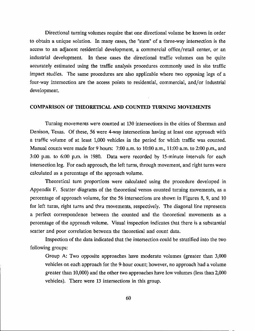
Directional turning volumes require that one directional volume be known in order
to obtain a unique solution. In many cases, the "stem" of a three-way intersection is the
access to an adjacent residential development, a commercial office/retail center, or an
industrial development. In these cases the directional traffic volumes can be quite
accurately estimated using the traffic analysis procedures commonly used in site traffic
impact studies. The same procedures are also applicable where two opposing legs of a
four-way intersection are the access points to residential, commercial, and/or industrial
development.
COMPARISON OF THEORETICAL AND COUNTED TURNING MOVEMENTS
Turning movements were counted at 130 intersections in the cities of Sherman and
Denison, Texas. Of these, 56 were 4-way intersections having at least one approach with
a traffic volume of at least 1,000 vehicles in the period for which traffic was counted.
Manual counts were made for 9 hours: 7:00 a.m. to 10:00 a.m., 11:00 a.m. to 2:00 p.m., and
3:00 p.m. to 6:00 p.m. in 1980. Data were recorded by IS-minute intervals for each
intersection leg. For each approach, the left turns, through movement, and right turns were
calculated as a percentage of the approach volume.
Theoretical turn proportions were calculated using the procedure developed in
Appendix F. Scatter diagrams of the theoretical versus counted turning movements, as a
percentage of approach volume, for the 56 intersections are shown in Figures 8, 9, and 10
for left turns, right turns and thru movements, respectively. The diagonal line represents
a perfect correspondence between the counted and the theoretical movements as a
percentage of the approach volume. Visual inspection indicates that there is a substantial
scatter and poor correlation between the theoretical and count data.
Inspection of the data indicated that the intersection could be stratified into the two
following groups:
Group A: Two opposite approaches have moderate volumes (greater than 3,000
vehicles on each approach for the 9-hour count; however, no approach had a volume
greater than 10,000) and the other two approaches have low volumes (less than 2,000
vehicles). There were 13 intersections in this group.
60
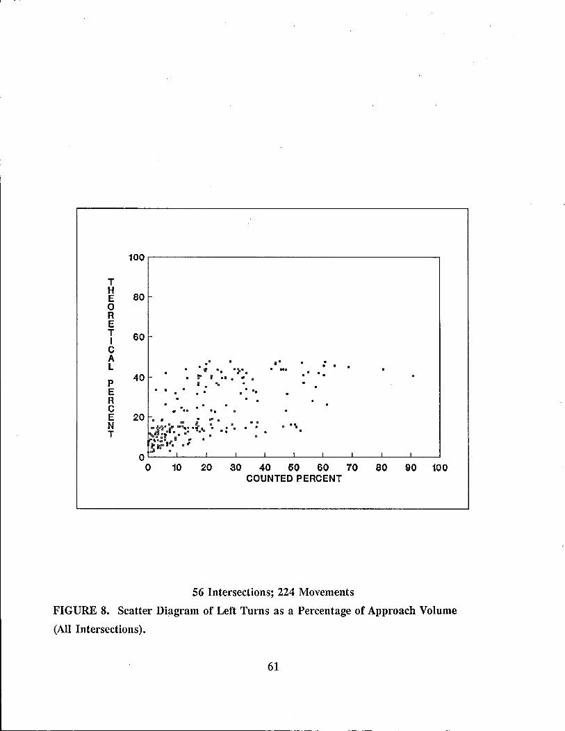
T H E o R E T I C A L
P E R C E N T
100.--------------------------------------------,
so
60
40
aD ,D, a a" DD D)D. a DO.
~ I •• a .. •
B a"" • ..
. . . ..
. '. .. . . . ."
. . . . . .
30 40 50 60 70 COUNTED PERCENT
56 Intersections; 224 Movements
so 90 100
FIGURE 8. Scatter Diagram of Left Turns as a Percentage of Approach Volume
(All Intersections).
61
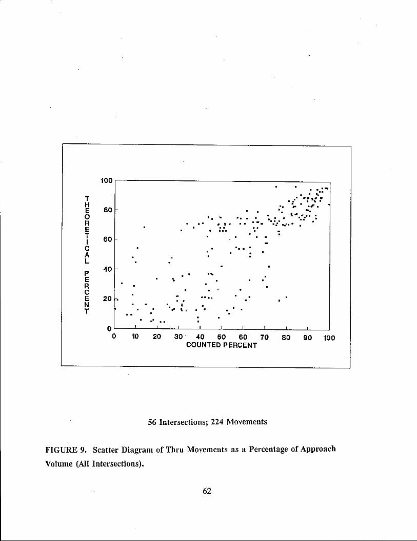
T H E o R E T I C A L
P E R C E N T
100r-------------------------------------~
80
60
40
20 .
o •
D aD. a
.. • I 0
o • . . ..
. a.:" 00 .. a· • II, ...
• • • 1\ • a. 0... ..,.
•• •• a.. , .. '.a a .... .. .. .
••• _ ••• : .. aDrJ' •• a.
... . o o
o 0 o • .
0L---L---~1--~ __ ~L_ __ L_ __ L_ __ ~ __ _L __ _L __ ~
o 10 20 30 40 50 60 70 COUNTED PERCENT
56 Intersections; 224 Movements
80 90 100
FIGURE 9. Scatter Diagram of Thru Movements as a Percentage of Approach
Volume (All Intersections).
62
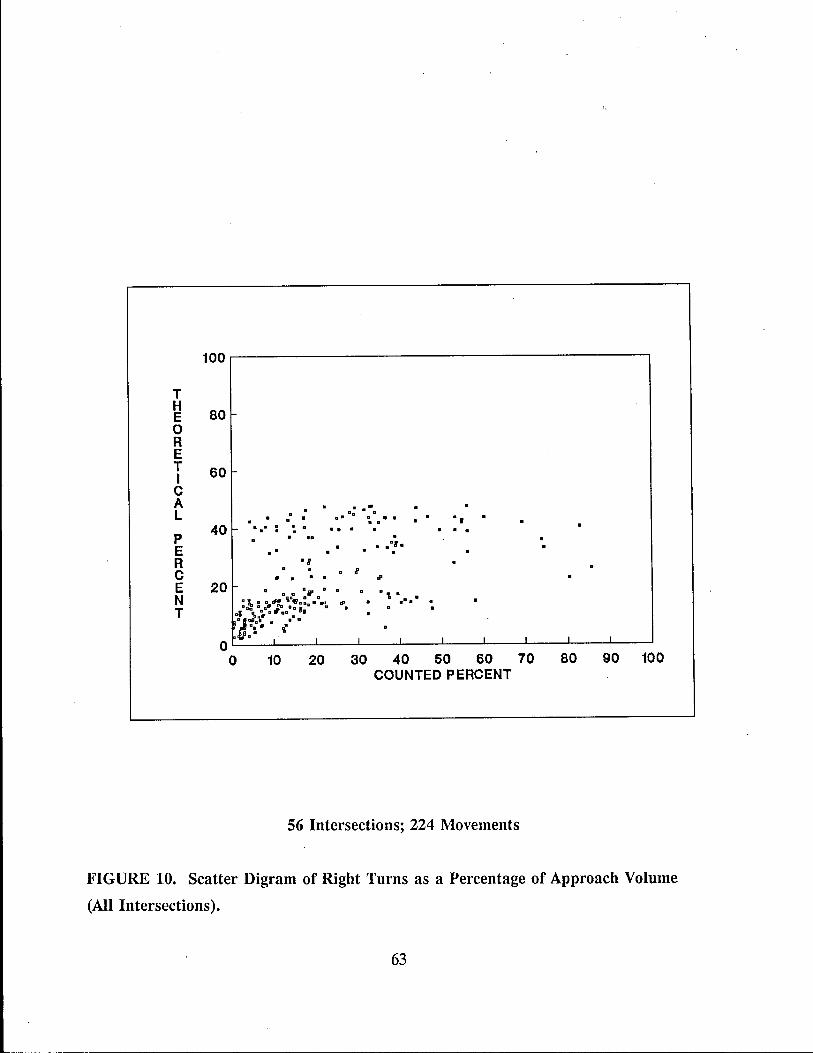
T H E o R E T I C A L
P E R C E N T
100.-----------------------------------------,
80
60
o • 0
40 r- •• D:' -:..
20
.. • .0
., o . . . .
.: a ....
D· -:. ••• ... . o ,
. . .. ,. . a a,. .
aa a a .
" . . .
56 Intersections; 224 Movements
FIGURE 10. Scatter Digram of Right Turns as a Percentage of Approach Volume
(All Intersections).
63
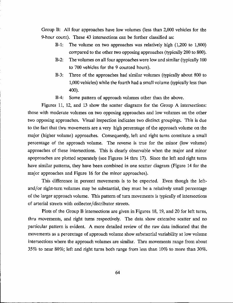
Group B: All four approaches have low volumes (less than 2,000 vehicles for the
9-hour count). These 43 intersections can be further classified as:
B-1: The volume on two approaches was relatively high (1,200 to 1,800)
compared to the other two opposing approaches (typically 200 to 800).
B-2: The volumes on all four approaches were low and similar (typically 100
to 700 vehicles for the 9 counted hours).
B-3: Three of the approaches had similar volumes (typically about 800 to
1,000 vehicles) while the fourth had a small volume (typically less than
400).
B-4: Some pattern of approach volumes other than the above.
Figures 11, 12, and 13 show the scatter diagrams for the Group A intersections:
those with moderate volumes on two opposing approaches and low volumes on the other
two opposing approaches. Visual inspection indicates two distinct groupings. This is due
to the fact that thru movements are a very high percentage of the approach volume on the
major (higher volume) approaches. Consequently, left and right turns constitute a small
percentage of the approach volume. The reverse is true for the minor (low volume)
approaches of these intersections. This is clearly observable when the major and minor
apoproaches are plotted separately (see Figures 14 thru 17). Since the left and right turns
have similar patterns, they have been combined in one scatter diagram (Figure 14 for the
major approaches and Figure 16 for the minor approaches).
This difference in percent movements is to be expected. Even though the left
and/or right-turn volumes may be substantial, they must be a relatively small percentage
of the larger approach volume. This pattern of turn movements is typically of intersections
of arterial streets with collector/distributor streets.
Plots of the Group B intersections are given in Figures 18, 19, and 20 for left turns,
thru movements, and right turns respectively. The data show extensive scatter and no
particular pattern is evident. A more detailed review of the raw data indicated that the
movements as a percentage of approach volume show substantial variability at low volume
intersections where the approach volumes are similar. Thru movements range from about
35 % to near 80%; left and right turns both range from less than 10% to more than 30%.
64
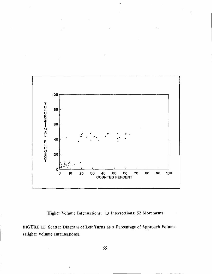
100
T H
80 E 0 R E T 60 I C A
" ," . L " . . .,
DD"
P 40
E R C E 20 N T
" a ':m: D. d' all""
" I I I I I I I I I 0 0 10 20 30 40 50 60 70 80 90 100
COUNTED PERCENT
Higher Volume Intersections: 13 Intersections; 52 Movements
FIGURE 11 Scatter Diagram of Left Turns as a Percentage of Approach Volume
(Higher Volume Intersections).
65
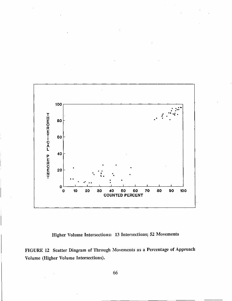
100 • _.: III . .
T . .. . 0 ·Ol •
H . 0 . .
E 80 I-0 R E T 60 I C A L
P 40
E R C E 20 N D H
0
T " 0
D DD o D D
0 I I I I I I I I I
0 10 20 30 40 50 60 70 80 90 100 COUNTED PERCENT
Higher Volume Intersections: 13 Intersections; 52 Movements
FIGURE 12 Scatter Diagram of Through Movements as a Percentage of Approach
Volume (Higher Volume Intersections).
66
T H E o R E T I C A L
P E R C E N T
100r-----------------------------__________ ~
80
60
40
20
. . . .
Ia.: •• a,,_ a. dI. a
OL---~---'L---~ __ ~I ____ L_ __ ~' __ ~'~ __ L_' __ ~I __ ~
o 10 20 30 40 50 60 70 80 90 COUNTED PERCENT
100
Higher Volume Intersections: 13 Intersections; 52 Movements
FIGURE 13 Scatter Diagram of Right Turns as a Percentage of Approach Volume
(Higher Volume Intersections).
67
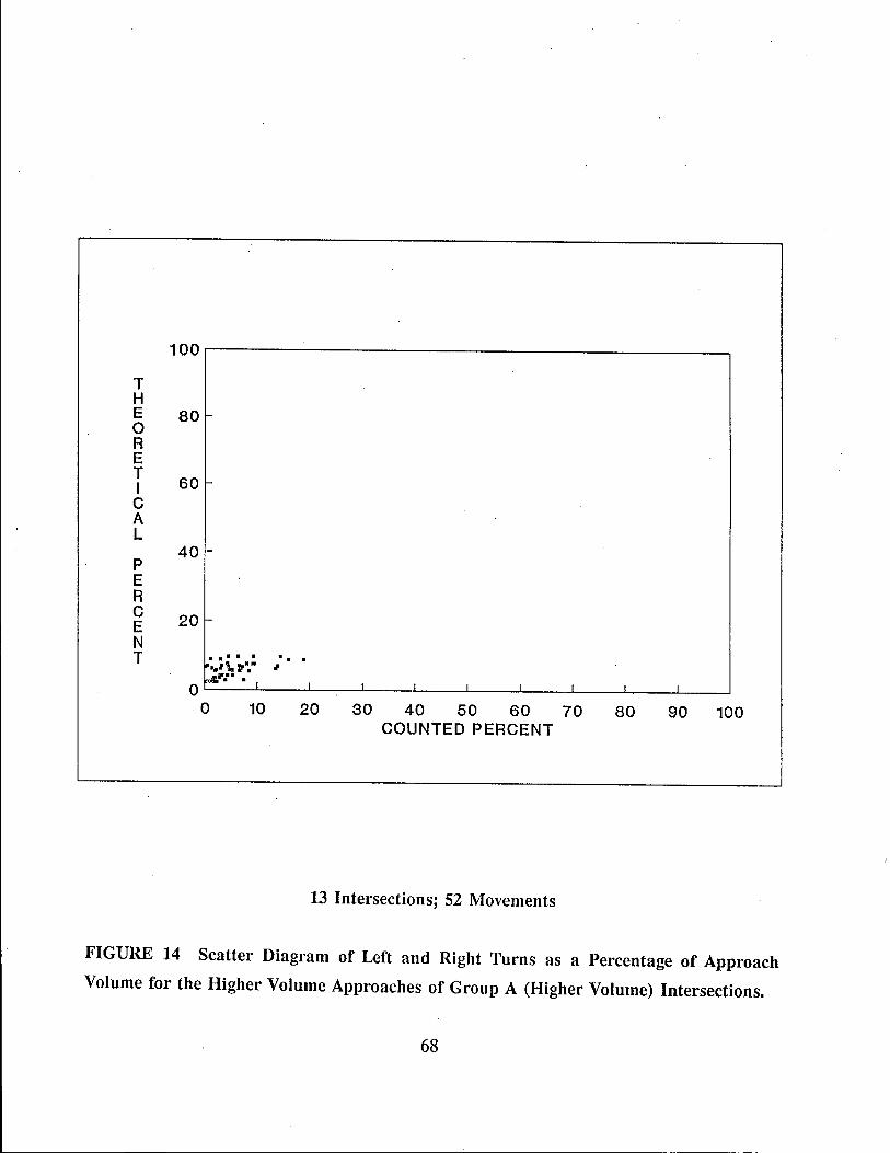
100~--------------------------------------------~
T H E 80 ~ o R E
T 60 f
C A L
P E R C E N T
40 ~
20 f-
. . ... ... 10-... , to 'to: ~
1..1.11'''" " I I I I I I I I O~--~---L--~----L---~--~ ____ L-__ ~ __ -L __ ~
o 10 20 30 40 50 60 70 COUNTED PERCENT
13 Intersections; S2 Movements
80 90 100
FIGURE 14 Scatter Diagram of Left and Right Turns as a Percentage of Approach
Volume for the Higher Volume Approaches of Group A (Higher Volume) Intersections.
68
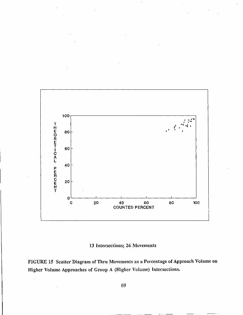
100 . . .... T
. . .. . .. . H · .~ . · . E 80
. · 0 R E T
60 I C A L
40 P E R C 20 E N T
0 I I I
0 20 40 60 80 100 COUNTED PERCENT
13 Intersections; 26 Movements
FIGURE 15 Scatter Diagram of Thru Movements as a Percentage of Approach Volume on
Higher Volume Approaches of Group A (Higher Volume) Intersections.
69
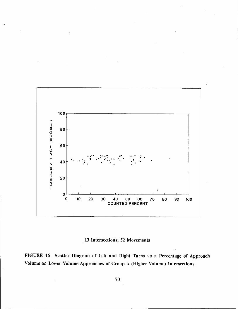
T H E o R E T I C A L
P E R C E N T
100.-------------------------------------------~
80 I-
60 I-
40 ..
20
. ... . ., . . . . . :- ... . . .- ... . •• .. . .. . . .
O~--~---L--~I----L-I--~ __ _L __ ~ ____ L_ __ ~ __ ~
o 10 20 30 40 50 60 70 COUNTED PERCENT
,13 Intersections; 52 Movements
80 90 100
FIGURE 16 Scatter Diagram of Left and Right Turns as a Percentage of Approach
Volume on Lower Volume Approaches of Group A (Higher Volume) Intersections.
70
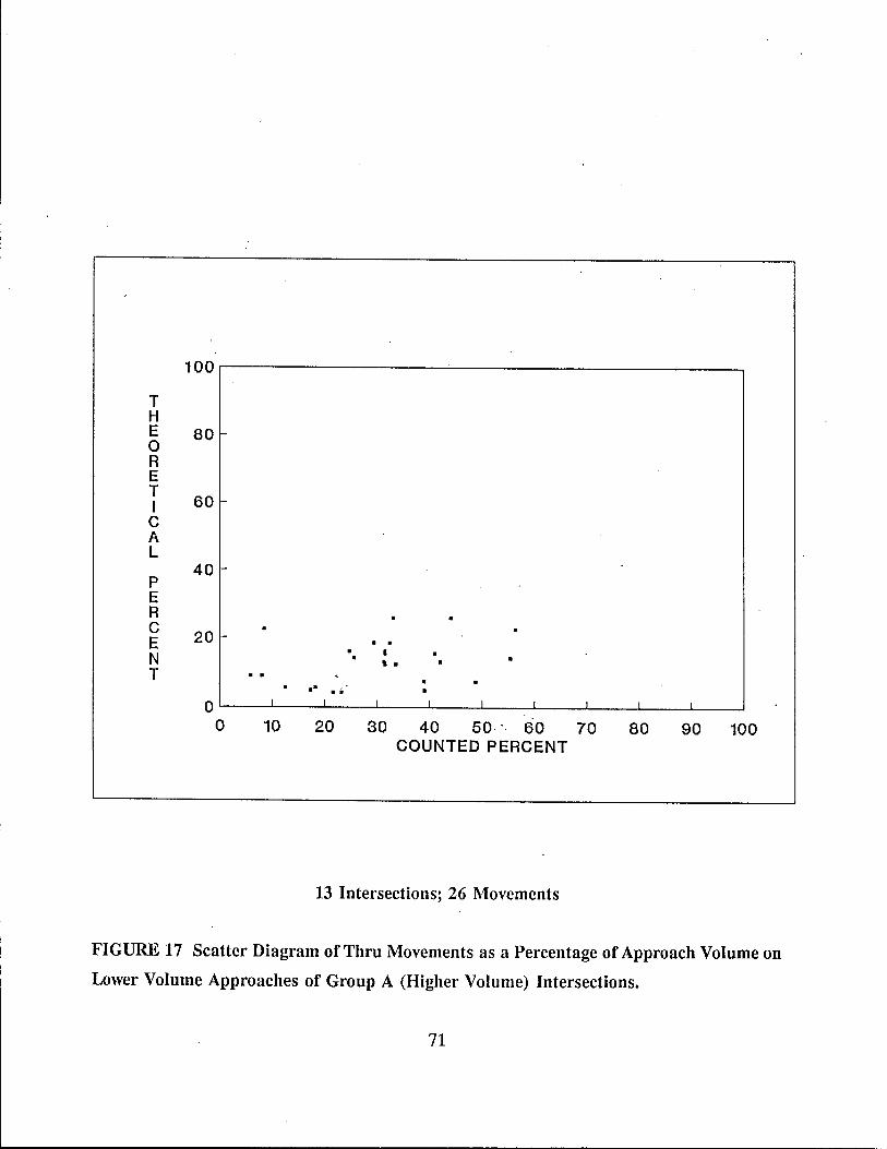
100
T H E 80 0 R E T 60 l-I C A L
40 I-P E R C 20 l-E . • N . , . T
.' •• 0 I I I 1 I I I I 1
0 10 20 30 40 50· - 60 70 80 90 100 COUNTED PERCENT
13 Intersections; 26 Movements
FIGURE 17 Scatter Diagram of Thru Movements as a Percentage of Approach Volume on
Lower Volume Approaches of Group A (Higher Volume) Intersections.
71
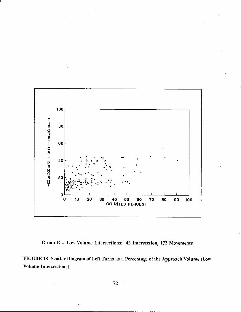
T H E o R E T I C A L
p E R C E N T
100r-------------------------------------------~
80
60
40 . ,. , .. • 0 ..
o • o 0
.. o ..
o 00
o • . .
-.
• 0"
OL---~--_L-I--~I--__ L-I __ ~I ____ ~ __ ~I ____ L_I __ ~I __ ~
o 10 20 30 40 50 60 70 80 90 100 COUNTED PERCENT
Group B -- Low Volume Intersections: 43 Intersection, 172 Movements
FIGURE 18 Scatter Diagram of Left Turns as a Percentage of the Approach Volume (Low
Volume Intersections).
72
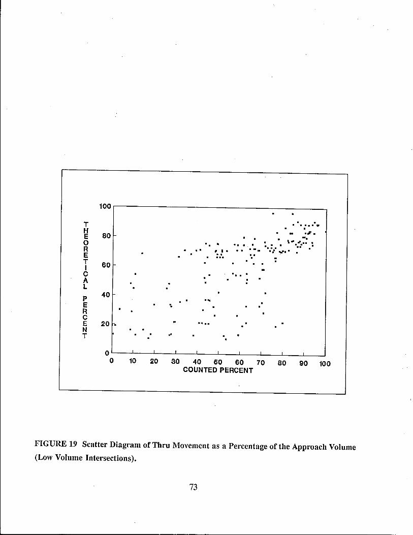
T H E o R E T I C A L
P E R C E N T
100r-----------------------________________ ~
80 !-
60
40 'L
20 .. I- ..
0 I I
0 10 20 30
. . .. . , . . . . . ..
... . ...
I
40 60
. . . . .... . ., . . . -. . , .. .... . .. ... ... .... . .• . -. • ..... ".p.. .
... . . .
60
. . . . .
I
70 I
80 I
90 COUNTED PERCENT
100
FIGURE 19 Scatter Diagram of Thru Movement as a Percentage of the Approach Volume
(Low Volume Intersections).
73
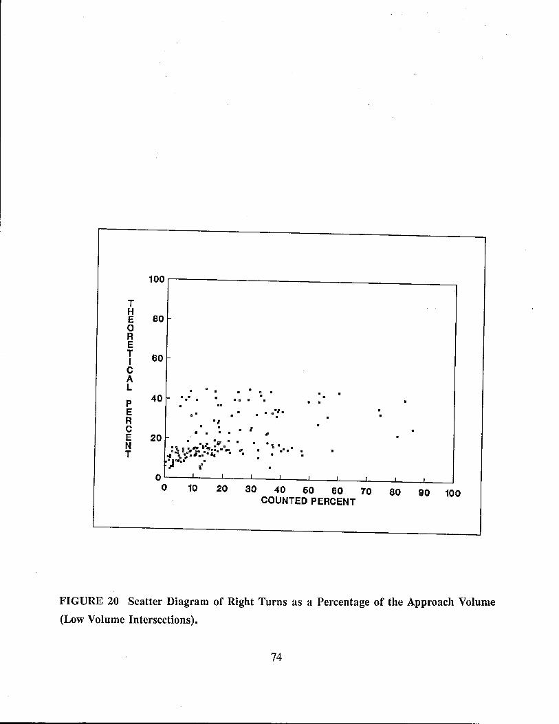
100~--------------____________________ ~
T H E SO o R E
T 60 C A L
P E R C E N T
40
20
. . . . . . ., . • . . .
. . .,0": •..
.~ : : .. ~ .:"aa. __ • aI J~ .••• B. :,I.. , ..
. . . . . . . . . . . a-I •
. , " . . . ,.. .
"'. . . .. . . . O~--~I~--L---~I----L-I--~ ___ L-I __ ~~ __ . __ L-__ ~IL-~
o 10 20 30 40 60 60 70 SO 90 100 COUNTED PERCENT
FIGURE 20 Scatter Diagram of Right Turns as a Percentage of the Approach Volume
(Low Volume Intersections).
74
While the four general patterns (B-1 thru B-4) identified above are apparent from
the raw data, subdivision into these groups for analysis did not appear to be worthwhile for
the purposes of this study due to the limited number of intersections in each of the
subgroups.
Figure 21 shows the distribution of the differences between the theoretical and
counted movements as a percent of approach volume (percent theoretical minus percent
by count) for the 13 higher volume (Group A) intersections. Hence, negative values
indicate an underestimate by the procedure for calculating the theoretical percentage. The
differences appear to be more or less symmetrically distributed. However, close inspection
indicates that the differences in the thru movements are skewed to positive differences.
Thus, the theoretical procedure tended to underestimate the thru movement and
overestimate left and right turns as a percent of approach volume.
Figure 22 shows the distribution of the difference in the theoretical and observed
turn percentages. The modal (most frequent) difference for thru movements is a minus
10%, for left and right turns it is plus 5%. This suggests that theoretical procedure tends
to underestimate thru movement percentages and overestimate turn movements where
intersection approach volumes are very small.
Statistical Analysis
F-tests at the 10% significance level were performed to determine if the variances
of the theoretical and observed percent left turns, thru movements and right turns are
significantly different.
The statistical data are summarized in Table 7. The numerical value of the variance
of the counted volume is larger than the theoretical values in all cases. This is to be
expected since the "real world" will experience some diversity, while the theoretical
procedure yields a unique solution for a given set of approach volumes. In all but two
cases, the alternate hypothesis was accepted: there is statistical evidence that the difference
in the variances is significant.
75
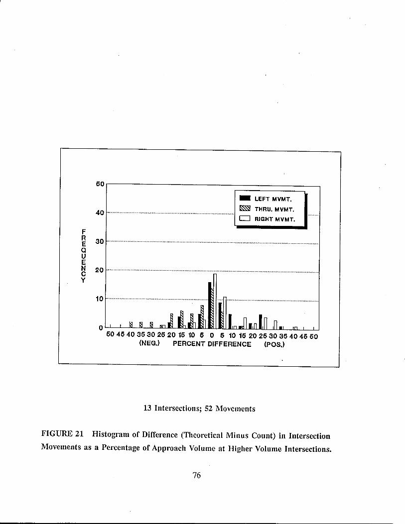
F R E Q U E N C Y
50r-----------------------------____________ ~
_ LEFT MVMT.
~ THRU. MVMT. 40 ................................................................................................ 0 RIGHT MVMT.
30 ................................................................................................................................................................. .
20 ................................................................................................................................................................ .
10 ............................................................................ . .......................................................................... .
O~~~~~~~~~~~~~~~~~~~~~~~
50 4540 3530 25 20 15 10 5 0 5 10 15 20 2530 354045 50 (NEG.) PERCENT DIFFERENCE (POS.)
13 Intersections; S2 Movements
FIGURE 21 Histogram of Difference (Theoretical Minus Count) in Intersection
Movements as a Percentage of Approach Volume at Higher Volume Intersections.
76
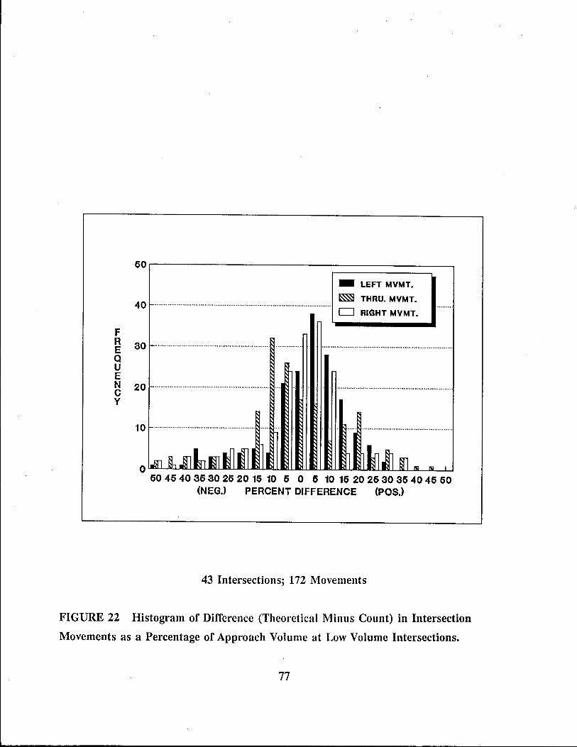
F R E Q U E
50r-------------------------------------------~
40 ............................................................................................... .
30 ............................................................................ .
_ LEFT MVMT.
~ THRU. MVMT.
D RIGHT MVMT.
N 20 ................................................................ . C Y
10 .............................................................. .
O~~~~~~u.~~~~~~~mu.u~~~Lm~~~
50 45 40 3530 25 20 15 10 5 0 5 10 15 20 2530 35 40 45 50 (NEG.) PERCENT DIFFERENCE (POS.)
43 Intersections; 172 Movements
FIGURE 22 Histogram of Difference (Theoretical Minus Count) in Intersection
Movements as a Percentage of Approach Volume at Low Volume Intersections.
77
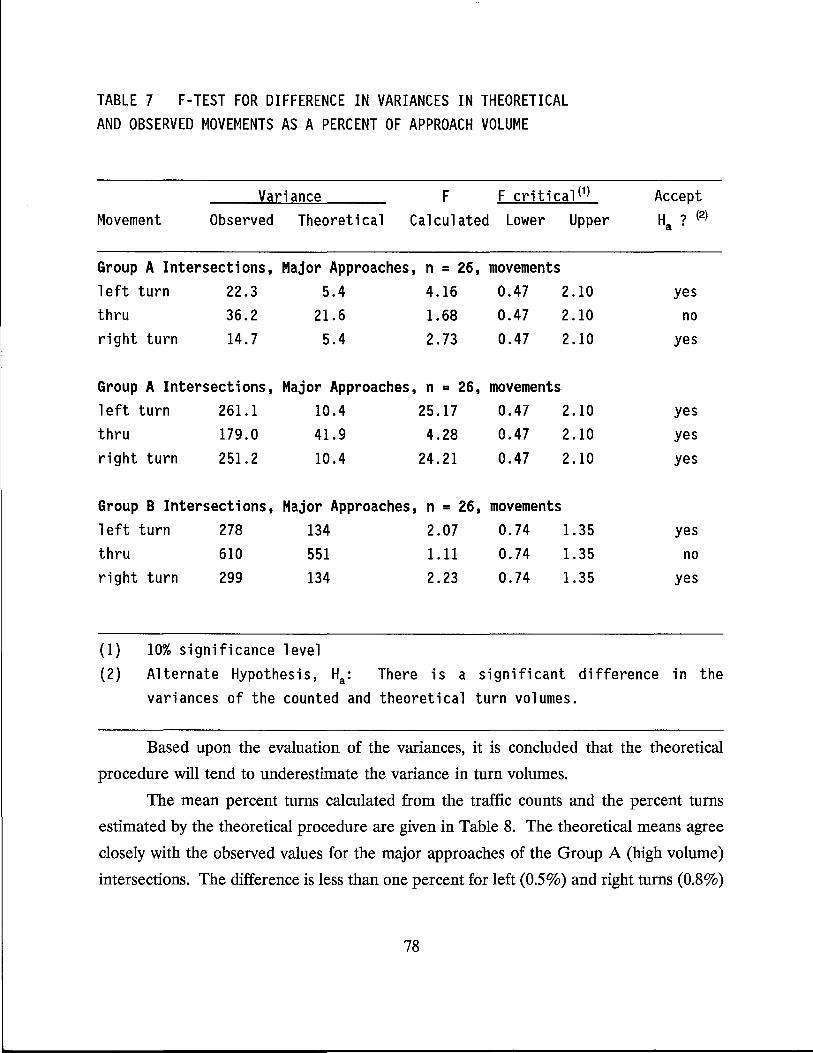
TABLE 7 F-TEST FOR DIFFERENCE IN VARIANCES IN THEORETICAL AND OBSERVED MOVEMENTS AS A PERCENT OF APPROACH VOLUME
Variance F F critical (1)
Movement Observed Theoretical Calculated Lower Upper
Group A Intersections, Major Approaches, n = 26, movements 1 eft turn 22.3 5.4 4.16 0.47 2.10 thru 36.2 21.6 1.68 0.47 2.10 right turn 14.7 5.4 2.73 0.47 2.10
Group A Intersections, Major Approaches, n = 26, movements 1 eft turn 261.1 10.4 25.17 0.47 2.10 thru 179.0 41.9 4.28 0.47 2.10 right turn 251.2 10.4 24.21 0.47 2.10
Group B Intersections, Major Approaches, n = 26, movements 1 eft turn 278 134 2.07 0.74 1.35 thru 610 551 1.11 0.74 1.35 right turn 299 134 2.23 0.74 1.35
(1) 10% significance level
Accept Ha ? (2)
yes no
yes
yes yes yes
yes no
yes
(2) Alternate Hypothesis, Ha: There is a significant difference in the variances of the counted and theoretical turn volumes.
Based upon the evaluation of the variances, it is concluded that the theoretical
procedure will tend to underestimate the variance in turn volumes.
The mean percent turns calculated from the traffic counts and the percent turns
estimated by the theoretical procedure are given in Table 8. The theoretical means agree
closely with the observed values for the major approaches of the Group A (high volume)
intersections. The difference is less than one percent for left (0.5%) and right turns (0.8%)
78
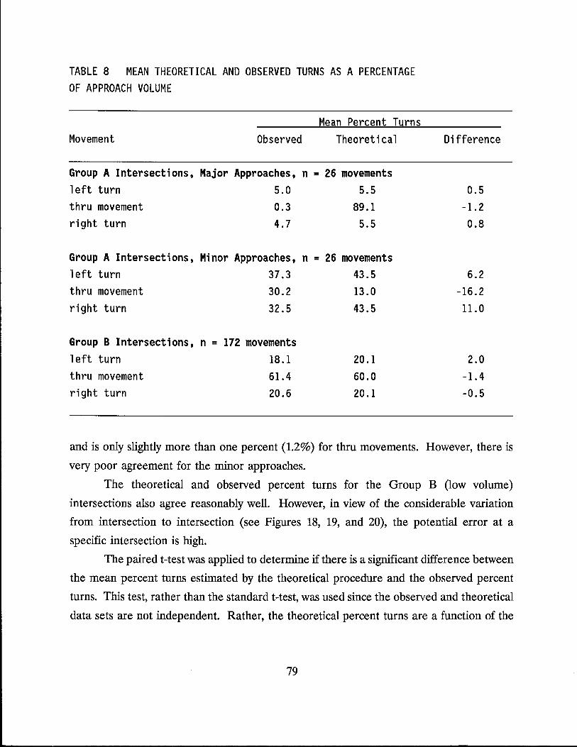
TABLE 8 MEAN THEORETICAL AND OBSERVED TURNS AS A PERCENTAGE OF APPROACH VOLUME
Mean Percent Turns Movement Observed Theoretical Difference
Group A Intersections, Major Approaches, n = 26 movements 1 eft turn 5.0 5.5 0.5 thru movement 0.3 89.1 -1.2 right turn 4.7 5.5 0.8
Group A Intersections, Minor Approaches, n = 26 movements 1 eft turn 37.3 43.5 6.2 thru movement 30.2 13.0 -16.2 right turn 32.5 43.5 11.0
Group B Intersections, n = 172 movements left turn 18.1 20.1 2.0 thru movement 61.4 60.0 -1.4 right turn 20.6 20.1 -0.5
and is only slightly more than one percent (1.2%) for thru movements. However, there is
very poor agreement for the minor approaches.
The theoretical and observed percent turns for the Group B (low volume)
intersections also agree reasonably well. However, in view of the considerable variation
from intersection to intersection (see Figures 18, 19, and 20), the potential error at a
specific intersection is high.
The paired t-test was applied to determine if there is a significant difference between
the mean percent turns estimated by the theoretical procedure and the observed percent
turns. This test, rather than the standard t-test, was used since the observed and theoretical
data sets are not independent. Rather, the theoretical percent turns are a function of the
79
approach volumes at a particular intersection. The paired t-test statistics are presented in
Table 9.
The alternate hypothesis was rejected for the major approaches at high volume
(Group A) intersections (there is a significant difference between the theoretical and
observed mean percent turns). Therefore it can be concluded that the mean percent turns
estimated by the theoretical procedure could be the same as the observed mean percent
turns. Inspection of Figures 14 and 15 shows that there is very little scatter in these data
points. Thus, it appears that the theoretical procedure produces a reliable estimate of
turning movement percentages for the major approaches of intersections where two
opposing approaches have high traffic volumes and the other two opposing approaches have
low volumes.
However, the two following limitations should be noted. First, this conclusion
applies to turning movements over the high traffic hours of the day. Since most of the daily
traffic in an urban area occurs during the hours for which traffic count data were collected,
it might be assumed that the theoretical percent turns are applicable to the 24-hour period.
However, there is no evidence to suggest that the procedure provides reliable estimates of
percent turns during specific times of the day (e.g., a.m. or p.m. peak hours).
80
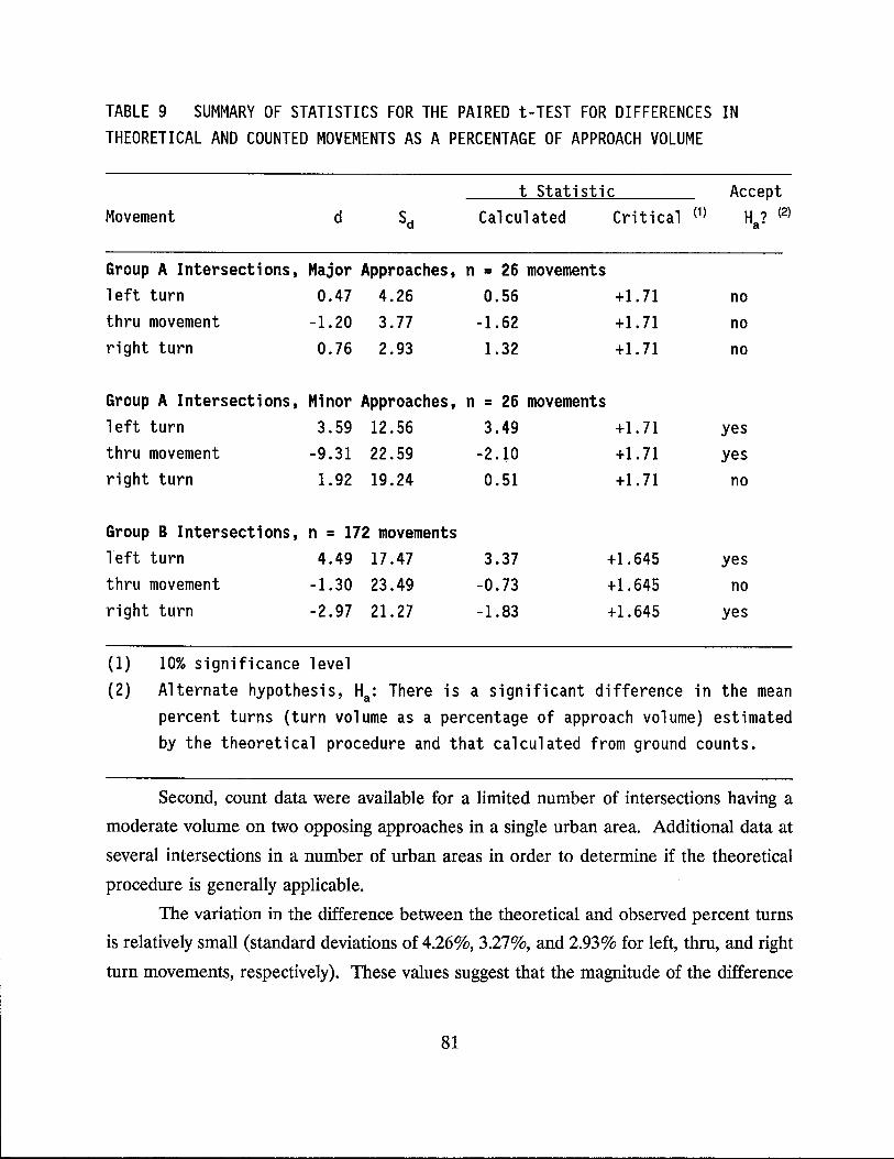
TABLE 9 SUMMARY OF STATISTICS FOR THE PAIRED t-TEST FOR DIFFERENCES IN THEORETICAL AND COUNTED MOVEMENTS AS A PERCENTAGE OF APPROACH VOLUME
t Statistic Accept Movement d Sd Calculated Critical (1) Ha? (2)
Group A Intersections, Major Approaches, n = 26 movements 1 eft turn 0.47 4.26 0.56 +1. 71 no thru movement -1.20 3.77 -1.62 +1. 71 no right turn 0.76 2.93 1.32 +1. 71 no
Group A Intersections, Minor Approaches, n = 26 movements 1 eft turn 3.59 12.56 3.49 +1. 71 yes thru movement -9.31 22.59 -2.10 +1. 71 yes right turn 1.92 19.24 0.51 +1. 71 no
Group B Intersections, n = 172 movements left turn 4.49 17 .47 3.37 +1.645 yes thru movement -1.30 23.49 -0.73 +1.645 no right turn -2.97 21.27 -1.83 +1.645 yes
(1) 10% significance level (2) Alternate hypothesis, Ha: There is a significant difference in the mean
percent turns (turn volume as a percentage of approach volume) estimated by the theoretical procedure and that calculated from ground counts.
Second, count data were available for a limited number of intersections having a
moderate volume on two opposing approaches in a single urban area. Additional data at
several intersections in a number of urban areas in order to determine if the theoretical
procedure is generally applicable.
The variation in the difference between the theoretical and observed percent turns
is relatively small (standard deviations of 4.26%, 3.27%, and 2.93% for left, thru, and right
turn movements, respectively). These values suggest that the magnitude of the difference
81
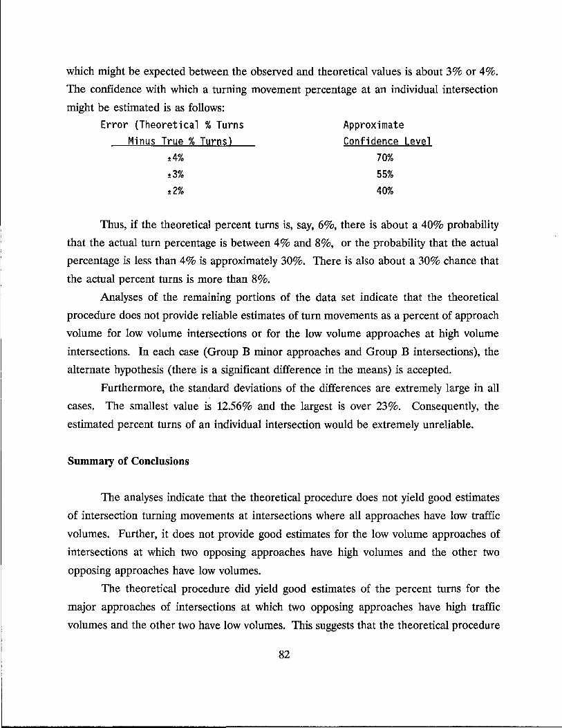
which might be expected between the observed and theoretical values is about 3% or 4%.
The confidence with which a turning movement percentage at an individual intersection
might be estimated is as follows:
Error (Theoretical % Turns Minus True % Turns)
±4% ±3% ±2%
Approximate Confidence Level
70% 55% 40%
Thus, if the theoretical percent turns is, say, 6%, there is about a 40% probability
that the actual turn percentage is between 4% and 8%, or the probability that the actual
percentage is less than 4% is approximately 30%. There is also about a 30% chance that
the actual percent turns is more than 8%.
Analyses of the remaining portions of the data set indicate that the theoretical
procedure does not provide reliable estimates of turn movements as a percent of approach
volume for low volume intersections or for the low volume approaches at high volume
intersections. In each case (Group B minor approaches and Group B intersections), the
alternate hypothesis (there is a significant difference in the means) is accepted.
Furthermore, the standard deviations of the differences are extremely large in all
cases. The smallest value is 12.56% and the largest is over 23%. Consequently, the
estimated percent turns of an individual intersection would be extremely unreliable.
Summary of Conclusions
The analyses indicate that the theoretical procedure does not yield good estimates
of intersection turning movements at intersections where all approaches have low traffic
volumes. Further, it does not provide good estimates for the low volume approaches of
intersections at which two opposing approaches have high volumes and the other two
opposing approaches have low volumes.
The theoretical procedure did yield good estimates of the percent turns for the
major approaches of intersections at which two opposing approaches have high traffic
volumes and the other two have low volumes. This suggests that the theoretical procedure
82
may be applicable to intersections where at least two of the four approaches have high
traffic volumes. Additional.research is essential to verify the results obtained with the very
limited data set which is available.
From a practical application standpoint, the need to forecast turn percentages, and
then turn volumes, involves intersections at which high traffic volumes are expected on at
least two approaches. There is little need to forecast individual movement at very low
volume intersections because the individual turn volumes will not affect the design. The
intersection geometries will be controlled by physical turning characteristics of the design
vehicle. Capacity will not be an issue since an intersection with minimum physical
characteristics can accommodate substantial volumes. And finally, intersections with very
low volumes on all approaches are local street/collector street connectors which are a
function of the subdivision or site development design. Even the intersection of two
collector/distributor facilities, site distance, and design vehicle characteristics, not the
volume of the various movements, will be the controlling factor.
Recommendations for Further Analyses
The theoretical procedure appears to have promise for estimating turning movements
at high volume intersections. In order to validate the procedure and to identify the range
of volumes over which it is valid, it is recommended that turning movement counts be made
at a number of intersections. The following list is in order of priority for data collection and
analysis:
1. All four approaches to the intersection are known to have high ADTs as well
as high volumes during the a.m. and p.m. peak periods. A nondirectional
ADT of at least 40,000 vpd on each of the four legs of the intersection is a
suggested minimum criterion for selection.
2. Two opposing approaches are known to have high ADTs as well as high
volumes in the a.m. and p.m. peak periods. An ADT of at least 40,000 vpd
on these two legs of the intersection is suggested. The other two approaches
83
should have moderate volumes. An ADT of at least 5,000 vpd on each of the
two lower volume approaches is suggested as a selection criterion.
3. All four approaches have similar volumes but of a lower magnitude than (1)
above. The suggested selection criterion is that the ADT on each of the four
intersection legs be between 20,000 and 30,000 vpd.
The following recommendations are made relative to the data collection:
1. The manual turning movement counts should be made for the period 6 a.m.
to at least 8 p.m.
2. The data should be summarized by IS-minute intervals. This will permit
identification of the highest volume 60-minute interval at each intersection
during the a.m. and p.m. peak periods. Thus the theoretical turn percentages
can be compared to the counted percentages for the a.m. peak hours, for
other selected hours of the day, and for the total count period.
3. In order to evaluate transferability of the results, data should be collected in
at least three different urban areas.
4. In order to provide a degree of statistical reliability, data should be collected
for at least 10 (preferably at least 30) intersections in each of the volume
categories in each city. For example, at 30 intersections where all approaches
are known to have high volumes (see (1) above) counts should be taken (Le.,
10 intersections x 3 urban areas). If all three volume categories are to be
evaluated, 90 intersections would need to be counted (Le., 3 categories x 10
intersections in each category x 3 urban areas).
84
CHAPTER V. RESTRAINT ASSIGNMENT USING EQUALIZED VIC RATIOS
Existing capacity restraint assignment procedures provide excellent results for
evaluating system-level alternatives and for analyzing transportation system plans. However,
refinement of the assignment results, such as that performed by the Corridor Analysis
Group of the Transportation Planning Section (D-lOP), is essential for project-level
planning. Such procedures are manual and therefore time-consuming.
Their research study developed and evaluated a computerized process which
equalizes the VIC ratios on competing routes. The logic of such an approach is as follows:
In a very detailed network there are a large number of possible paths between two points
which are some distance apart. Several of these possible paths have similar total
impedances (total centroid-to-centroid travel time). Each of the similar paths should
accommodate some of the trips. And the distribution of traffic on these paths should result
in VIC ratios which are equal or nearly equal.
Such a procedure should more closely reflect actual trip-making characteristics when
the coded network is in such detail that it has, or nearly has, a one-to-one correspondence
to the actual street system. Therefore, the procedure equalizing VIC ratios should produce
more realistic turning movement volumes.
STUDY PROCEDURES
Testing of the assignment procedures to equalize the VIC ratios on competing
routes involved the following elements:
1. Formulation of the procedure
2. Development of the prototype microcomputer software
3. Selection and coding of a test network
4. Analysis of the results
Formulation of Procedures
The procedures for equalizing the VIC ratios on competing routes involve two
85
elements. The first is to be able to identify the links which comprise competing routes.
This was easily accomplished since the TRANPLAN package utilizes a two-digit field for
link classification. Different numbers in this field were used to identify the various links
in the different competing routes for the purposes of testing and evaluating the concept of
equalizing V Ie ratios. If the procedure was found to be effective, the TRANPLAN
package would be modified to establish a unique field for identifying competing routes. The
present link classification field would then be used for the traditional functional
classification purposes.
The second element is to determine the impedance adjustment function. It was
hypothesized that this function should have the properties indicated in Figure 23. If the
V Ie ratios of a link are equal to the average V Ie for given competing routes, the adjusted
impedance should be the same as the previous impedance. If the link V Ie is greater than
or less than average, the impedance should be increased. Further, the magnitude of the
adjustment should increase as the ratio of the link V Ie to the average V Ie becomes more
distant from 1.0.
Development of Software
The existing TRANPLAN package was modified to incorporate a technique to
equalize the V Ie ratios. This involved development of two subroutines. The first was for
calculating the average V Ie ratios for all links on competing routes. The second subroutine
calculated the adjusted link impedances. The relationship between the subroutines and the
main TRANPLAN program is indicated in Figure 24. Figure 25 shows the subroutine
structure for calculating the average V Ie ratio. The procedure for modifying the existing
HLOD5 subroutine in TRANPLAN is shown in Figure 26. Figure 25 shows the existing
BPR formula used to update the impedance on those links which are not competing routes
within the project-level area and on links outside of the project area.
86
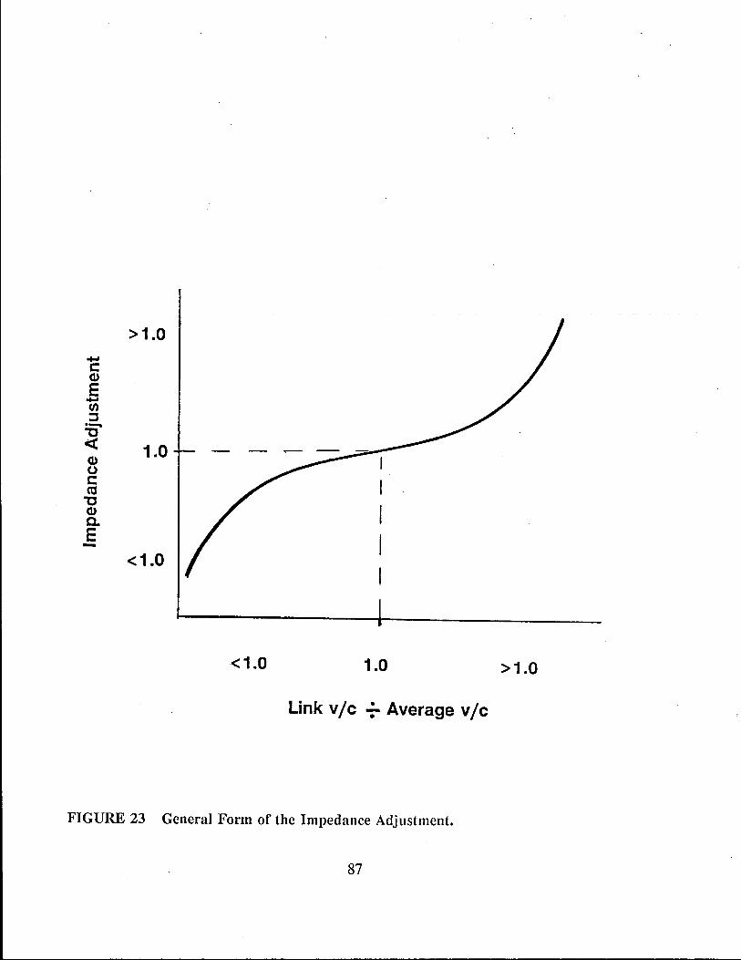
>1.0 .... s: Q)
E ..... (J) ::J .-
"C « 1.0 Q) 0 s: ctS
"C Q) c. E -
<1.0
<1.0 1.0 >1.0
Link vie -:- Average vie
FIGURE 23 General Form of the Impedance Adjustment.
87
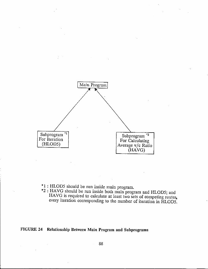
Subprogram *1
For Iteration (HLOD5)
Subprogram *2
For Calculating Average v / c Ratio
(HAVG)
* 1 : HLOD5 should be run inside main program. *2 : HA VG should be run inside both main program and HLOD5; and
HA VG is required to calculate at least two sets of competing routes, every iteration corresponding to the number of iteration in HLOD5.
FIGURE 24 Relationship Between Main Program and Subprograms
88
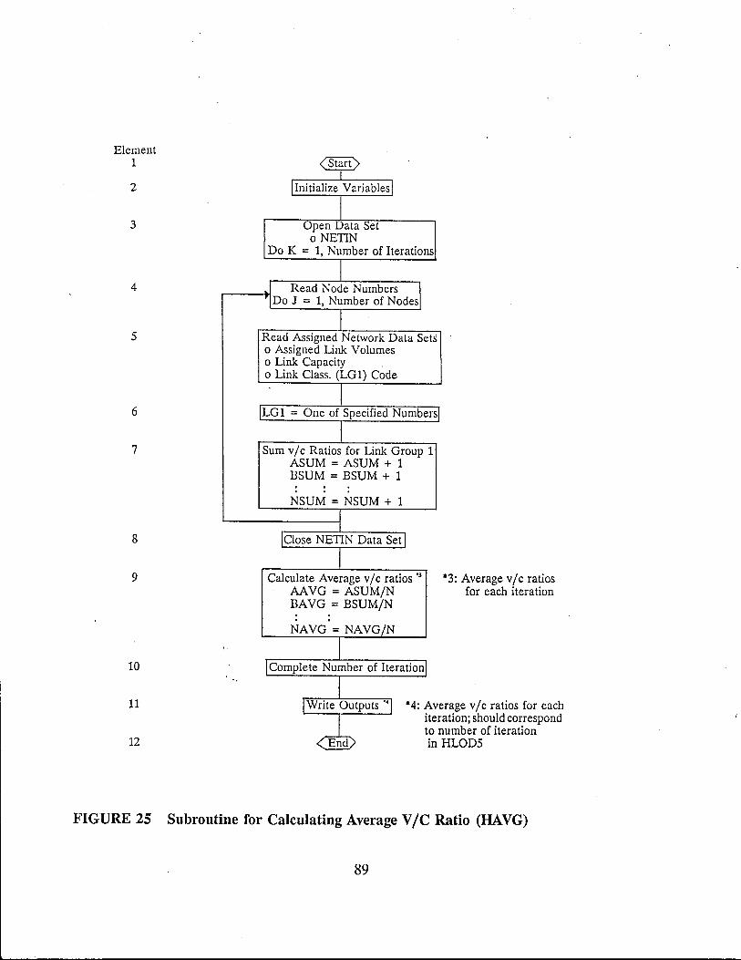
Element 1
2
3
4
5
6
7
8
9
10
,.
<Start> ~
I lni tialize Variables I
I Open Data Set
o NETIN Do K = 1, Number of Iterations
I .1 Read Node Numbers sl 'IDo J = 1, Number of Nodes
I Read Assigned Network Data Sets o Assigned Link Volumes o Link Capacity o Link Class. (LG 1) Code
1 LGI = One of Specified Numbers
I Sum v I c Ratios for Link Group 1
ASUM = ASUM + 1 BSUM = BSUM + 1 : : :
NSUM = NSUM + 1 -r l
[Close NETIN Data Set I
1 Calculate Average vic ratios '3
AAVG = ASUM/N BA VG = BSUM/N : :
NAVG = NAVG/N
T I Complete Number of Iteration
j
*3: Average vic ratios for each iteration
I Write Outputs '41 *4: Ave 11 rage vic ratios for each iter ation; should correspond
umber of iteration to n ~ in 12 HLOD5
FIGURE 25 Subroutine for Calculating Average VIC Ratio (HA VG)
89
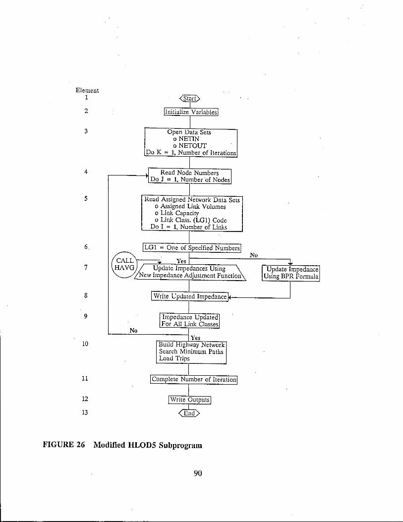
Element 1
2
3 Open Data Sets o NETIN o NETOUT
Do K = 1, Number of Iterations
4 Read Node Numbers Do J = 1, Number 'of Nodes
5 Read Assigned Network Data Sets o Assigned Link Volumes o Link Capacity o Link Class. (LGl) Code
Do I = 1, Number of Links
6 LG 1 = One of Specified Numbers No
Yes 7 Update Impedances Using
New Impedance Adjustment Function
8 Write Updated Impedance
9
No Yes
10 Build Highway Network Search Minimum Paths Load Trips
11 Complete Number of Iteration
12
13
FIGURE 26 Modified HLOD5 Subprogram
90
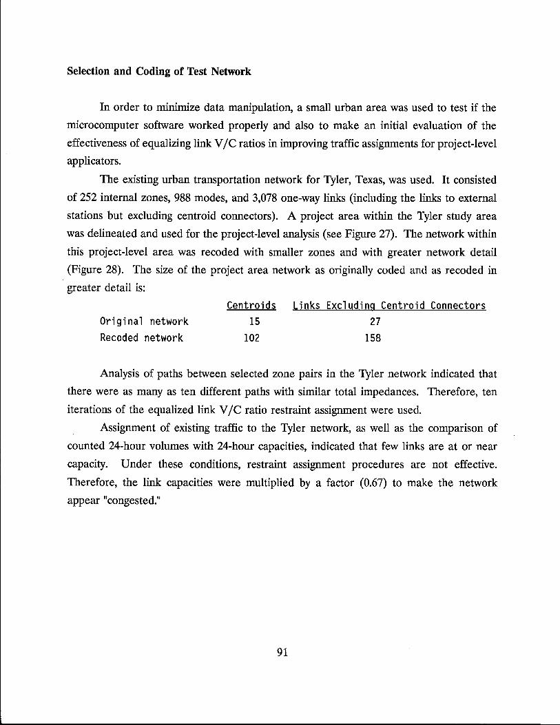
Selection and Coding of Test Network
In order to minimize data manipulation, a small urban area was used to test if the
microcomputer software worked properly and also to make an initial evaluation of the
effectiveness of equalizing link V Ie ratios in improving traffic assignments for project-level
applicators.
The existing urban transportation network for Tyler, Texas, was used. It consisted
of 252 internal zones, 988 modes, and 3,078 one-way links (including the links to external
stations but excluding centroid connectors). A project area within the Tyler study area
was delineated and used for the project-level analysis (see Figure 27). The network within
this project-level area was recoded with smaller zones and with greater network detail
(Figure 28). The size of the project area network as originally coded and as recoded in
greater detail is:
Original network Recoded network
Centroids 15
102
Links Excluding Centroid Connectors 27
158
Analysis of paths between selected zone pairs in the Tyler network indicated that
there were as many as ten different paths with similar total impedances. Therefore, ten
iterations of the equalized link V Ie ratio restraint assignment were used.
Assignment of existing traffic to the Tyler network, as well as the comparison of
counted 24-hour volumes with 24-hour capacities, indicated that few links are at or near
capacity. Under these conditions, restraint assignment procedures are not effective.
Therefore, the link capacities were multiplied by a factor (0.67) to make the network
appear "congested."
91
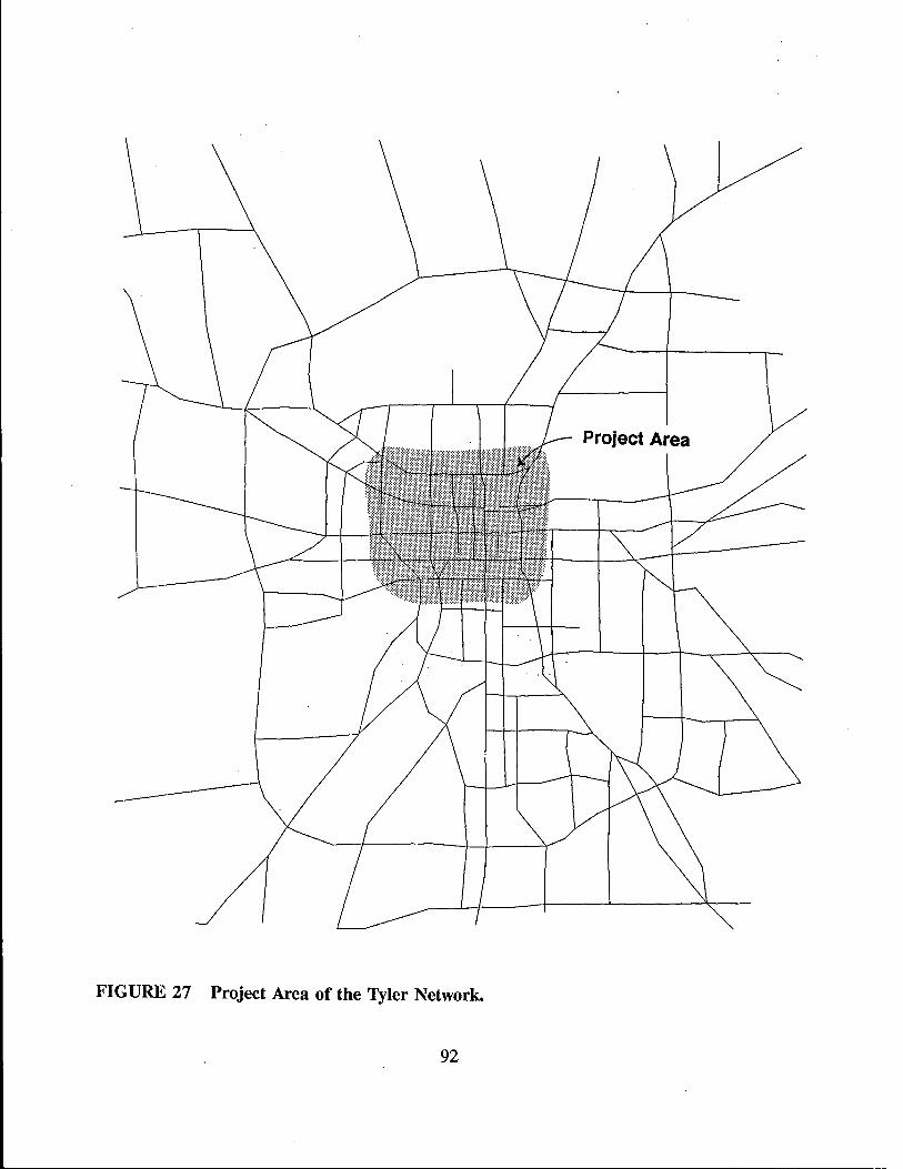
FIGURE 27 Project Area of the Tyler Network.
92
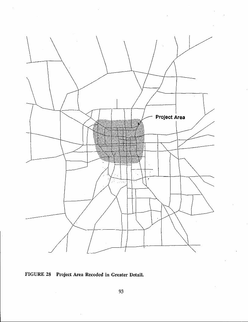
Project Area
................................................ ..... ........... .... ...... ' ..................... .
..... ', .............. . .... .....
FIGURE 28 Project Area Recoded in Greater Detail.
93
ANALYSIS
Analysis of the equalized V / C ratio assignment procedure involved the two following
principal evaluations:
1. Convergence of the link V /C ratios on competing routes to the average V /C
ratio for these routes; and
2. Improvement in turning movements compared to results using the existing
restraint assignment procedures.
Convergence of Link VIC Ratios
The concept of this restraint assignment is that the link V / C ratios on competing
routes should converge toward the mean value for each class/category of routes within the
project-level area. For the evaluation, 16 individual links, 4 cutlines, and 3 travel routes
were selected inside the project area (see Figure 29). The assignment results were
produced for from 1 to 10 iterations for both a congested network and a congested and
detailed network using the improved assignment technique which equalizes the link V /C
ratio.
Selected Links
There were three sets of competing routes inside the project area. One set was
comprised of four competing east-west major streets, the second was a pair of major north
south streets, and the third was two north-south collector streets. The pattern of link V /C
ratios from iteration to iteration was considered to be a major criterion of satisfactory
performance.
The data required for evaluation had to be extracted manually. Therefore, two links
on each of the routes were selected for determining if the desired closure of the V /C ratios
was being obtained. Table 10 contains the link V /C ratios for each of the 10 iterations.
The average V /C ratio for each link group is also given for each iteration. Visual
inspection shows that the V /C ratios do, in fact, converge toward the average for each link
94
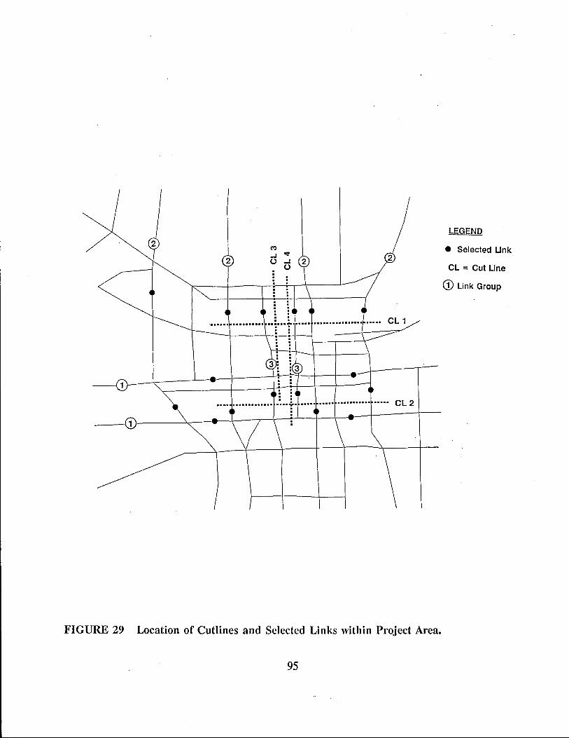
· · . · · · · . .•••••. •••••••••• •• ;, ••• ; ••••• •.••..•••.•.•.•. ••••• CL 1
· ·
CL2
FIGURE 29 Location of Cutlines and Selected Links within Project Area.
95
LEGEND
• Selected Link
CL = Cut Line
CD Link Group
group. This trend is especially noticeable for link groups 1 and 3. The standard errors, s,
are observed to systematically decrease as well.
Table 11 shows the link V Ie ratios for the same selected links in the more detailed.
Again, the individual link V Ie ratios "closed" on the average V Ie ratio of all links in each
group. However, the average V Ie ratios for each link group are somewhat lower than in
Table 10. This results because the more detailed network offers more paths through the
network. This in turn results in lower assigned volumes on the selected links. Inspection
of Table 11 indicates that the standard error on the tenth iteration is less than on the first.
However, the pattern of the diverse is not as "smooth" as for the original network (Table
10).
The F-test was performed to determine if the variance on the tenth iteration was
significantly less than on the first iteration. The equalized link vie ratio method was
expected to produce link V Ie ratios which converge toward the average V Ie ratio for each
group; hence, the variance should decrease. Therefore a one-tail test was employed; all
tests were made at the 10% significance level. As shown in Table 12, the F-test for
differences in variances, S2, indicated that the reduction from the first to the tenth iteration
is statistically significant at the 10% significance level for link groups 1 and 2 for the
original network. The reduction in the variance from the first to the tenth iteration was not
statistically significant (at the 10% significance level) for link group 3. Similar results were
achieved with the more detailed network. The reduction in the variance, S2, for link groups
1 and 2 is statistically significant at the 10% significance level. However, the reduction is
not statistically significant for link group 3.
The links in Groups 3 are on two north-south collector-type facilities which are
entirely within the project area. The very limited continuity of these routes restricts the
opportunity for path diversion from iteration to iteration. Therefore, there is limited
opportunity for the variation in the group V Ie ratios to decrease. Nevertheless, inspection
of Tables 10 and 11 shows that the variation in link V Ie ratios tends to decrease with
successive iterations for this group of links as well as for the Group 1 and 2 links.
96
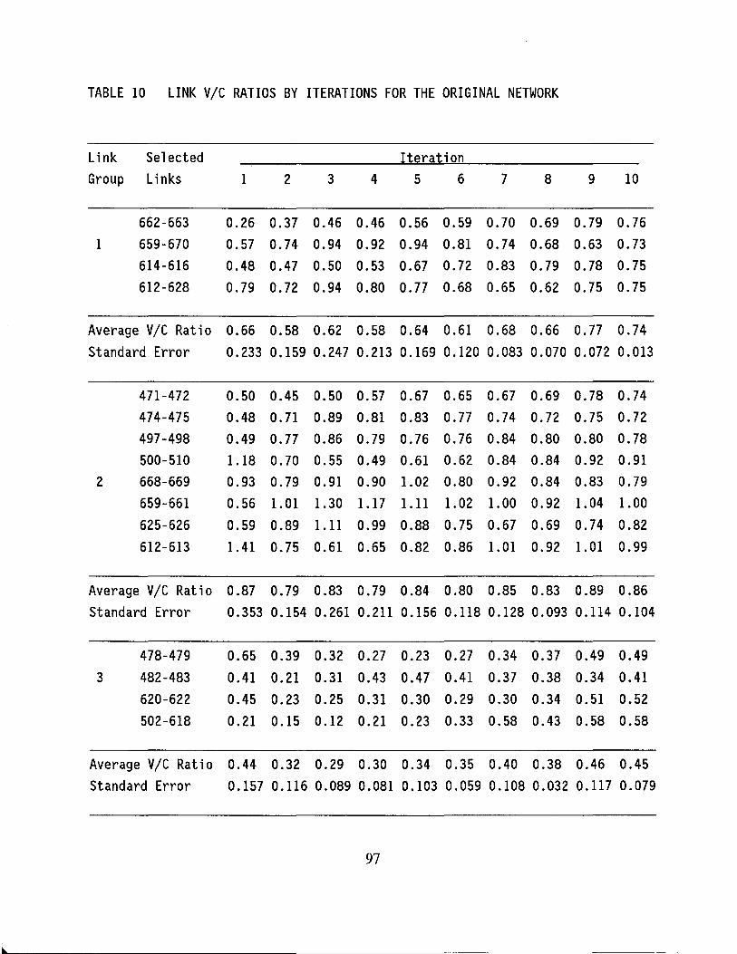
TABLE 10 LINK VIC RATIOS BY ITERATIONS FOR THE ORIGINAL NETWORK
Link Selected Iteration Group Links 1 2 3 4 5 6 7 8 9 10
662-663 0.26 0.37 0.46 0.46 0.56 0.59 0.70 0.69 0.79 0.76 1 659-670 0.57 0.74 0.94 0.92 0.94 0.81 0.74 0.68 0.63 0.73
614-616 0.48 0.47 0.50 0.53 0.67 0.72 0.83 0.79 0.78 0.75 612-628 0.79 0.72 0.94 0.80 0.77 0.68 0.65 0.62 0.75 0.75
Average VIC Ratio 0.66 0.58 0.62 0.58 0.64 0.61 0.68 0.66 0.77 0.74
Standard Error 0.233 0.159 0.247 0.213 0.169 0.120 0.083 0.070 0.072 0.013
471-472 0.50 0.45 0.50 0.57 0.67 0.65 0.67 0.69 0.78 0.74 474-475 0.48 0.71 0.89 0.81 0.83 0.77 0.74 0.72 0.75 0.72 497-498 0.49 0.77 0.86 0.79 0.76 0.76 0.84 0.80 0.80 0.78 500-510 1.18 0.70 0.55 0.49 0.61 0.62 0.84 0.84 0.92 0.91
2 668-669 0.93 0.79 0.91 0.90 1.02 0.80 0.92 0.84 0.83 0.79
659-661 0.56 1.01 1.30 1.17 1.11 1.02 1.00 0.92 1.04 1.00
625-626 0.59 0.89 1.11 0.99 0.88 0.75 0.67 0.69 0.74 0.82
612-613 1.41 0.75 0.61 0.65 0.82 0.86 1.01 0.92 1.01 0.99
Average VIC Ratio 0.87 0.79 0.83 0.79 0.84 0.80 0.85 0.83 0.89 0.86 Standard Error 0.353 0.154 0.261 0.211 0.156 0.118 0.128 0.093 0.114 0.104
478-479 0.65 0.39 0.32 0.27 0.23 0.27 0.34 0.37 0.49 0.49
3 482-483 0.41 0.21 0.31 0.43 0.47 0.41 0.37 0.38 0.34 0.41
620-622 0.45 0.23 0.25 0.31 0.30 0.29 0.30 0.34 0.51 0.52
502-618 0.21 0.15 0.12 0.21 0.23 0.33 0.58 0.43 0.58 0.58
Average VIC Ratio 0.44 0.32 0.29 0.30 0.34 0.35 0.40 0.38 0.46 0.45 Standard Error 0.157 0.116 0.089 0.081 0.103 0.059 0.108 0.032 0.117 0.079
97
l
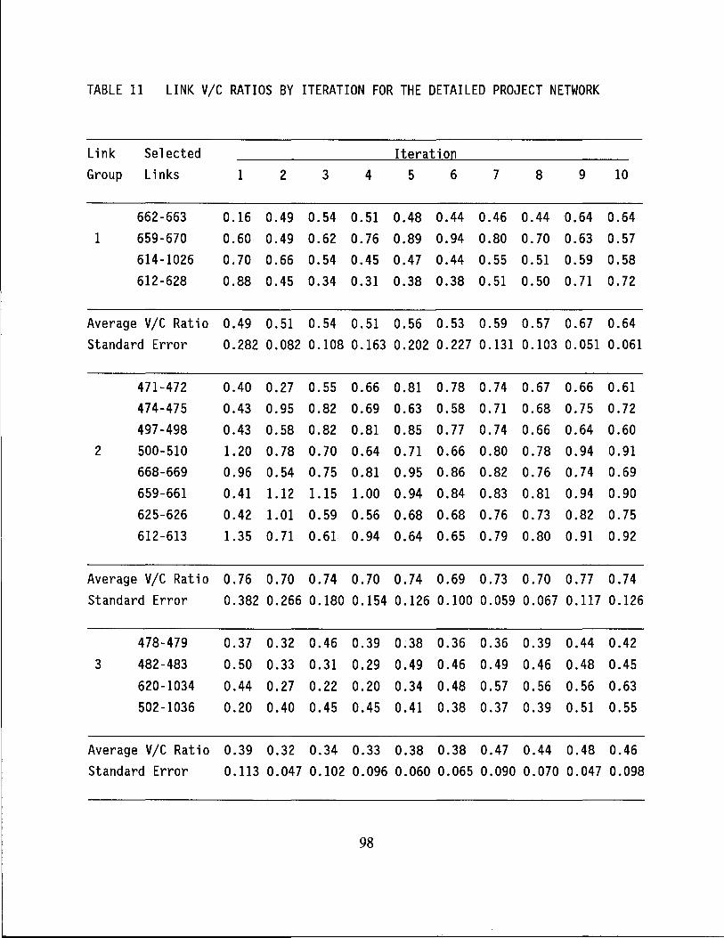
TABLE 11 LINK VIC RATIOS BY ITERATION FOR THE DETAILED PROJECT NETWORK
Link Selected Iteration Group Links 1 2 3 4 5 6 7 8 9 10
662-663 0.16 0.49 0.54 0.51 0.48 0.44 0.46 0.44 0.64 0.64 1 659-670 0.60 0.49 0.62 0.76 0.89 0.94 0.80 0.70 0.63 0.57
614-1026 0.70 0.66 0.54 0.45 0.47 0.44 0.55 0.51 0.59 0.58 612-628 0.88 0.45 0.34 0.31 0.38 0.38 0.51 0.50 0.71 0.72
Average VIC Ratio 0.49 0.51 0.54 0.51 0.56 0.53 0.59 0.57 0.67 0.64 Standard Error 0.282 0.082 0.108 0.163 0.202 0.227 0.131 0.103 0.051 0.061
471-472 0.40 0.27 0.55 0.66 0.81 0.78 0.74 0.67 0.66 0.61 474-475 0.43 0.95 0.82 0.69 0.63 0.58 0.71 0.68 0.75 0.72 497-498 0.43 0.58 0.82 0.81 0.85 0.77 0.74 0.66 0.64 0.60
2 500-510 1.20 0.78 0.70 0.64 0.71 0.66 0.80 0.78 0.94 0.91 668-669 0.96 0.54 0.75 0.81 0.95 0.86 0.82 0.76 0.74 0.69 659-661 0.41 1.12 1.15 1.00 0.94 0.84 0.83 0.81 0.94 0.90 625-626 0.42 1.01 0.59 0.56 0.68 0.68 0.76 0.73 0.82 0.75 612-613 1.35 0.71 0.61 0.94 0.64 0.65 0.79 0.80 0.91 0.92
Average VIC Ratio 0.76 0.70 0.74 0.70 0.74 0.69 0.73 0.70 0.77 0.74 Standard Error 0.382 0.266 0.180 0.154 0.126 0.100 0.059 0.067 0.117 0.126
478-479 0.37 0.32 0.46 0.39 0.38 0.36 0.36 0.39 0.44 0.42 3 482-483 0.50 0.33 0.31 0.29 0.49 0.46 0.49 0.46 0.48 0.45
620-1034 0.44 0.27 0.22 0.20 0.34 0.48 0.57 0.56 0.56 0.63 502-1036 0.20 0.40 0.45 0.45 0.41 0.38 0.37 0.39 0.51 0.55
Average VIC Ratio 0.39 0.32 0.34 0.33 0.38 0.38 0.47 0.44 0.48 0.46 Standard Error 0.113 0.047 0.102 0.096 0.060 0.065 0.090 0.070 0.047 0.098
98
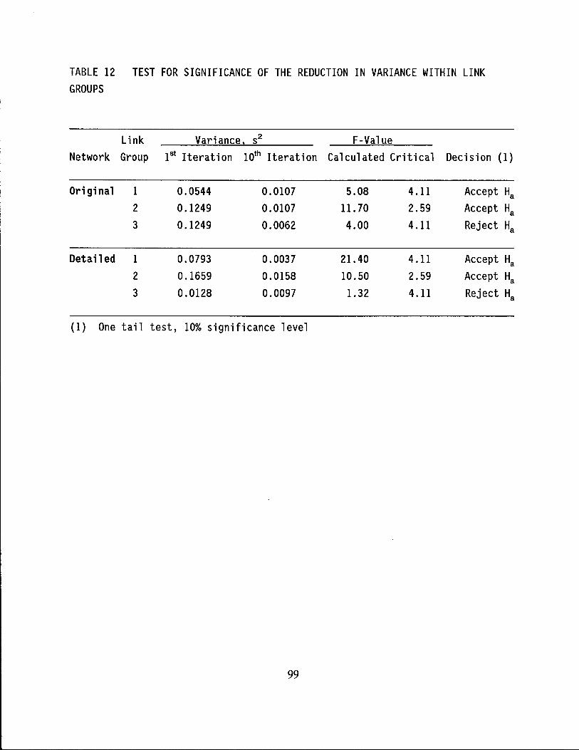
TABLE 12 TEST FOR SIGNIFICANCE OF THE REDUCTION IN VARIANCE WITHIN LINK GROUPS
Link Vari ance 2 S2 F-Value Network Group 1st Iteration 10th Iteration Calculated Critical Decision (1)
Original 1 0.0544 0.0107 5.08 4.11 Accept Ha 2 0.1249 0.0107 11.70 2.59 Accept Ha 3 0.1249 0.0062 4.00 4.11 Reject Ha
Detailed 1 0.0793 0.0037 21.40 4.11 Accept Ha 2 0.1659 0.0158 10.50 2.59 Accept Ha 3 0.0128 0.0097 1.32 4.11 Reject Ha
(1) One tail test, 10% significance level
99
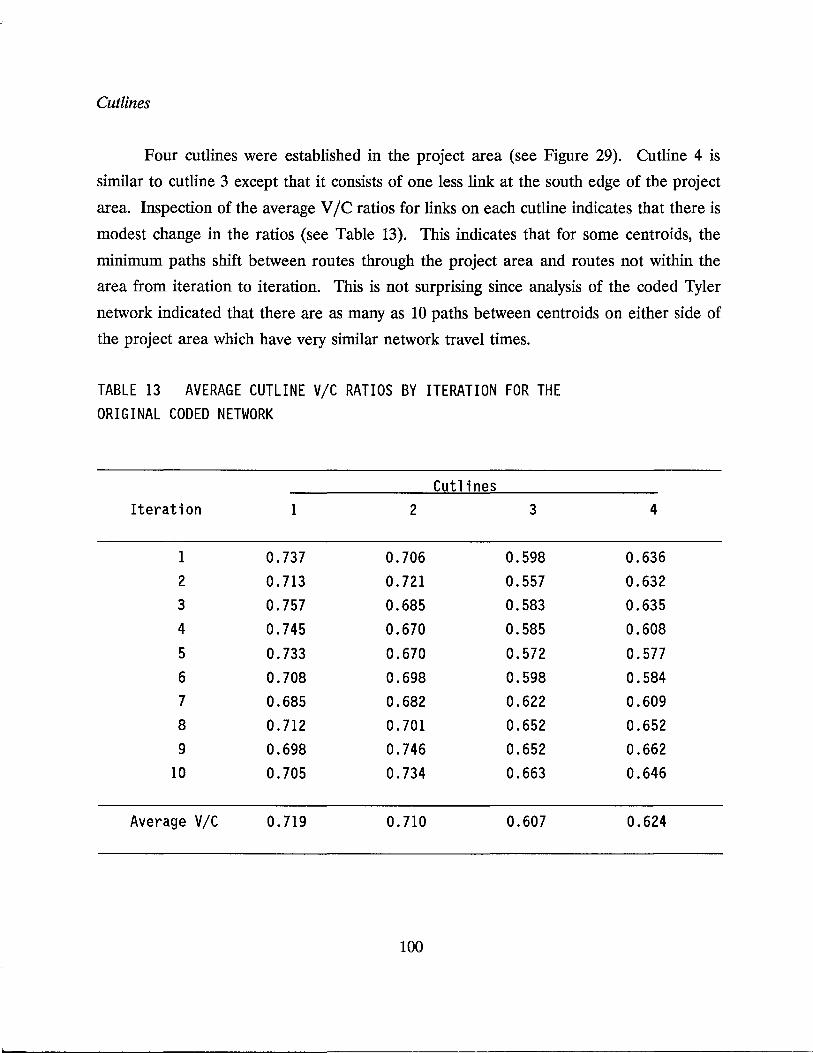
Cutlines
Four cutlines were established in the project area (see Figure 29). Cutline 4 is
similar to cutline 3 except that it consists of one less link at the south edge of the project
area. Inspection of the average V Ie ratios for links on each cutline indicates that there is
modest change in the ratios (see Table 13). This indicates that for some centroids, the
minimum paths shift between routes through the project area and routes not within the
area from iteration to iteration. This is not surprising since analysis of the coded Tyler
network indicated that there are as many as 10 paths between centroids on either side of
the project area which have very similar network travel times.
TABLE 13 AVERAGE CUTLINE VIC RATIOS BY ITERATION FOR THE ORIGINAL CODED NETWORK
Cutlines Iteration 1 2 3
1 0.737 0.706 0.598 2 0.713 0.721 0.557 3 0.757 0.685 0.583 4 0.745 0.670 0.585 5 0.733 0.670 0.572 6 0.708 0.698 0.598 7 0.685 0.682 0.622 8 0.712 0.701 0.652 9 0.698 0.746 0.652
10 0.705 0.734 0.663
Average VIC 0.719 0.710 0.607
100
4
0.636 0.632 0.635 0.608 0.577 0.584 0.609 0.652 0.662 0.646
0.624
Comparison of Assigned Turning Movements
The ideal evaluation of assignment procedures equalizing the vIc ratios on
competing routes would be to compare the assigned turning movements with counted
volumes. Since counted turning movements were not available, the assignment volumes
were compared to the results which were produced by the existing assignment procedure.
This procedure was judged to produce the best results when compared to mid-block count
data. The incremental procedure was selected as producing better results than the
stochastic, iterative,and equilibrium procedures. Four equal incremental loadings were
used. Four iterations were also used for the iterative and equilibrium techniques when
evaluating the existing restraint assignment techniques.
The following comparisons of the equalized link VIC ratio method and the
incremental assignment were made:
1. The Tyler Urban Transportation Study network in the detail as coded was
used. The link capacities were reduced as previously indicated to cause the
network to react as a "congested" network.
2. That portion of the network within the project area was recoded in greater
detail; the detail of the network outside of the project area remained
unchanged. The link capacities as previously factored to make the network
appear "congested" were used.
Because turning movement counts were not available, the following were used to
evaluate the potential improvement of the equalized VIC ratio method Gudged to provide
better results) over the existing capacity-restraint procedure:
1. Number of zero turning movements.
2. Distribution of the turning movements as a percentage of the approach
volume.
3. Paired t-test for difference in mean turn percentages.
The equalized link VIC ratio method did not produce a significant difference in the
number of zero turning movements (see Table 14). There were 5 left-turn and 4 right
turn movements having zero volume within the project area with the incremental
assignment. The equalized VIC ratio produced 3 left turns and 4 right turns having zero
101
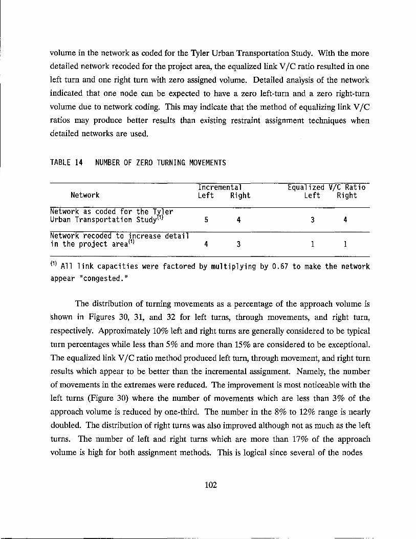
volume in the network as coded for the Tyler Urban Transportation Study. With the more
detailed network recoded for the project area, the equalized link VIC ratio resulted in one
left turn and one right turn with zero assigned volume. Detailed analysis of the network
indicated that one node can be expected to have a zero left-turn and a zero right-turn
volume due to network coding. This may indicate that the method of equalizing link VIC
ratios may produce better results than existing restraint assignment techniques when
detailed networks are used.
TABLE 14 NUMBER OF ZERO TURNING MOVEMENTS
Network
Network as coded for the Tyler Urban Transportation Study(1)
Network recoded to increase detail in the project area0)
Incremental Left Right
5 4
4 3
Equalized VIC Ratio Left Right
3 4
1 1
(1) All link capacities were factored by multiplying by 0.67 to make the network appear "congested."
The distribution of turning movements as a percentage of the approach volume is
shown in Figures 30, 31, and 32 for left turns, through movements, and right turn,
respectively. Approximately 10% left and right turns are generally considered to be typical
turn percentages while less than 5 % and more than 15% are considered to be exceptional.
The equalized link VIC ratio method produced left turn, through movement, and right turn
results which appear to be better than the incremental assignment. Namely, the number
of movements in the extremes were reduced. The improvement is most noticeable with the
left turns (Figure 30) where the number of movements which are less than 3% of the
approach volume is reduced by one-third. The number in the 8% to 12% range is nearly
doubled. The distribution of right turns was also improved although not as much as the left
turns. The number of left and right turns which are more than 17% of the approach
volume is high for both assignment methods. This is logical since several of the nodes
102
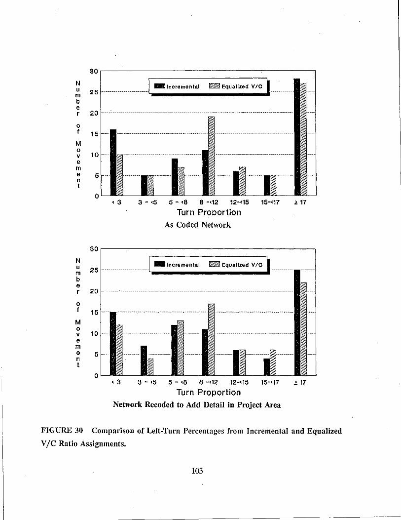
N u m b e r
o f
M o v e m e n t
N u m b e r
0 f
M 0 v e m e n t
30~------------------------------~--------~
J • Incremental - Equalized VIC I , .... , ......... " .. , ....... ' 251· .... · .... ' ...... ·' .. · .. ··· .. ·· .. ' .. ····"·' .. ··· ............ ·~ ____________________ .I ...... ,
20~ ............. " .. : .................. , ............................ , .. , .......... " .. , .. , ........... " ....... , .... , .............. " .................................... ~ ... ' ....... " ..... " .................. - ... " ........................... ".c." .................... , ..... ..
151--.. ..
10~ ...... I~·· .... ··· .... · .. ···· .. ····,·· .. · .... ···········"'·· .. · .. ,,·--.... · ..... , .... " ... ~~~' .............. ' ............ ' .. --" ................. " ....................... , .. " ............................. .
, @j ~ rd\\\\, ....................... ,
5"- ~ r I i~ ~ o L- .=-..--
< 3
30
25
20
15
10
5
0
3 - <5 5 - <8 8 -<12 12-<15
Turn ProDortion
As Coded Network
15-<17
• Incremental _ Equalized VIC
I· ..........
t ..........
t ..........
< 3 3 - <5 5 - <8 8 -<12 12-<15 15-<17 ~ 17
Turn Proportion
Network Recoded to Add Detail in Project Area
FIGURE 30 Comparison of Left-Turn Percentages from Incremental and Equalized
VIC Ratio Assignments.
103
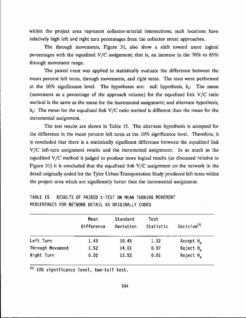
within the project area represent collector-arterial intersections; such locations have
relatively high left and right turn percentages from the collector street approaches.
The through movements, Figure 31, also show a shift toward more logical
percentages with the equalized vIc assignment; that is, an increase in the 70% to 85%
through movement range.
The paired t-test was applied to statistically evaluate the difference between the
mean percent left turns, through movements, and right turns. The tests were performed
at the 10% significance level. The hypotheses are: null hypothesis, ho: The mean
(movement as a percentage of the approach volume) for the equalized link VIC ratio
method is the same as the mean for the incremental assignment; and alternate hypothesis,
ha: The mean for the equalized link VIC ratio method is different than the mean for the
incremental assignment.
The test results are shown in Table 15. The alternate hypothesis is accepted for
the difference in the mean percent left turns at the 10% significance level. Therefore, it
is concluded that there is a statistically significant difference between the equalized link
VIC left-turn assignment results and the incremental assignment. In as much as the
equalized VIC method is judged to produce more logical results (as discussed relative to
Figure 31) it is concluded that the equalized link VIC assignment on the network in the
detail originally coded for the Tyler Urban Transportation Study produced left turns within
the project area which are significantly better than the incremental assignment.
TABLE 15 RESULTS OF PAIRED t-TEST ON MEAN TURNING MOVEMENT PERCENTAGES FOR NETWORK DETAIL AS ORIGINALLY CODED
Mean Standard Test Difference Deviation Statistic
Left Turn 1.43 10.45 1.32 Through Movement 1.52 14.01 0.97 Right Turn 0.02 13.52 0.01
(1) 10% significance level, two-tail test.
104
Decision(1)
Accept Ha Reject Ha Reject Ha
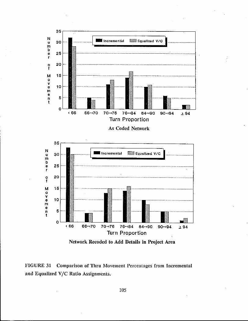
35r-----------------------------------------~--~
N u 30 m b e 25 r
o 20 f
M 15 o v e 10 m e n 5 t
o
........ __ ......•.......... __ . __ . ___ .1 - Incremental - Equalized VIC • ___ .. _________ . __ ..... __ . __ .. __ .. ___ .... _.1
( 66 66-<70 70-<76 76-<84 84-<90 90-<94 .l. 94
Turn Proportion
As Coded Network
35r------------------------------------------.
N u 30 m b e 25 r
o 20 f
M 15 o v e 10 m e n 5 t
o
- Incremental _ Equalized VIC
< 66 66-<70 70-<76 76-<84 84-<90 90-<94 ..l 94
Turn Proportion
Network Recoded to Add Details in Project Area
FIGURE 31 Comparison of Thru Movement Percentages from Incremental
and Equalized VIC Ratio Assignments.
105
However, the alternate hypothesis for both through movements and right turns is
rejected at the 10% significance level. Therefore, it is concluded that the mean turn
percentages for these movements could be the same for the equalized link VIC ratio and
incremental assignment methods. In other words, there is no statistically significant
difference between the mean through and right turn volumes as a percentage of the
approach volume. However, while the means are not significantly different for the right
turns, the distribution (see Figure 32) is certainly improved. Therefore, it is concluded that
the equalized link VIC ratio method did produce improved right turn results.
The improvement in the distribution of the percent through movement is less
dramatic than for left turns. Nevertheless, the equalized link,v I C ratio results are more
logical. Further, since it is concluded that the equalized VIC ratio method produced better
left and right turn movements, the through movement must also be improved.
Conclusions
Based upon the analysis of the assignment results obtained with the prototype
equalized link VIC ratio restraint assignment, the following conclusions and observations
are made:
1. The assignment process does perform as intended. Namely, the VIC ratios
for links in each link group converge toward the average VIC ratio for the
group.
2. The variation in the VIC ratios within each link group is reduced appreciably
even though the reduction may not be statistically significant.
3. Cutline VIC ratios did not change appreciably from iteration to iteration.
This indicates that while there was some movement of trips between rates
through the project area and rates outside the project area, the number of
trips was not large. The shifting that did occur appears to be reasonable for
the network (i.e., analysis of reasonable alternative paths indicated that as
many as 10 different paths may have very similar centroid-to-centroid travel
times).
4. The equalized link VIC ratio restraint assignment produced fewer turn
movements with zero volume within the project area.
106
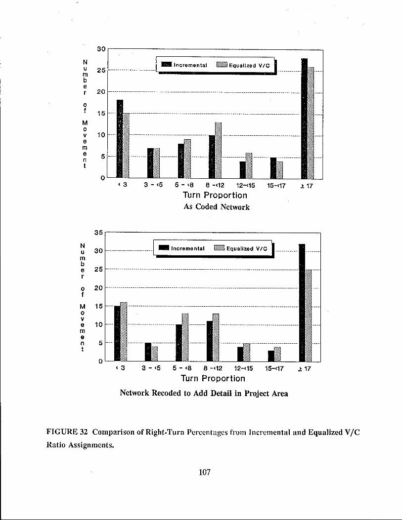
30,---------------------------------------------~
N _ Incremental _ Equalized VIC ~ 25 r····················································· .......... ~ ___________ ................................... .
b e r 20~········· ....................................................................................................... , ............................... .
o f
M o V e m e n t
15
10
5
o < 3 3 - <5 5 - <8 8 -<12 12-<15 15-<17 l. 17
Turn Proportion As Coded Network
35,--------------------------------------------. N u m b
30 1-..................................................... ···1 _ Incremental _ Equalized VIC
~------------------~ e 25r··················································· .......................•.•..•..••••.•............•....•....••.•.........................•..• _ ......................................................... .
r o 201-··················································· ........................................................................................................................ .
f
M 15 o v e 10 m e n 5 t
o < 3 3 - <5 5 - <8 8 -<12 12-<15 15-<17
Turn Proportion
Network Recoded to Add Detail in Project Area
.l. 17
FIGURE 32 Comparison of Right-Turn Percentages from Incremental and Equalized VIC
Ratio Assignments.
107
5. Evaluation of the distribution of turning movements as a percentage of
approach volume indicates that the equalized link V Ie ratio restraint
assignment produces results which are more reasonable than the existing
incremental restraint assignment. By inference it would also produce more
logical results than the other existing restraint assignment procedures since
the incremental procedure was judged to produce better results when the
existing techniques were compared.
108

CHAPTER VI. SUMMARY, CONCLUSIONS AND RECOMMENDATIONS
The traditional transportation modeling process (trip generation, trip distribution,
and traffic assignment) is an excellent tool for evaluation of land-use/transportation
alternatives. However, it is generally recognized that such a system level must be refined
for project-level applications. NCHRP Report 225 is the most exhaustive documentation
of procedures used to refine system-level traffic forecasts for use at the corridor or facility
level. Such procedures involve considerable judgment and must be performed by an
experienced analyst. Moreover, they are time-consuming and expensive.
A restraint assignment procedure which considers groups of links is hypothesized
to provide assignment results that are more applicable to project-level applications than
assignments obtained by existing techniques. The simplest approach is to equalize the link
V /C ratios on competing routes. This research project investigated the potential of such
a procedure. The research also included the investigation of manual corridor analysis
procedures and microcomputer applications which would facilitate the conduct of such
corridor studies.
There is a critical need to obtain traffic counts at intersections in order to provide
a data base for evaluating corridor analysis procedures and project-level traffic assignment
techniques.
CONCLUSIONS
The following is a summary of the conclusions drawn from this research project:
1. Intersection movements, as a percentage of approach volume, may be
calculated using a theoretical procedure based upon the relative conflicting
volumes. Good correlation between the theoretical and counted percent
turns was obtained for high volume approaches. The correlation was very
poor where all four approaches were low volume. Also, the theoretical values
did not compare favorably with the counted data for the low-volume
approaches where the other two opposing approaches were moderate to high
volume.
109
2. The prototype assignment procedure equalizing link vIc ratios on competing
routes functions as intended. That is, the vIc ratio of links of the same
classification do converge toward the average vIc ratio for the link class as
the number of iterations increases.
3. The prototype restraint assignment procedure produced better project-level
results than the existing incremental capacity-restraint assignment procedure.
Since the incremental procedure was judged to produce better results than
the stochastic, iterative, and equilibrium capacity-restraint assignment
methods, it is implied that the equalized link vIc ratio method would also
produce better project-level assignments than the other existing methods on
the Tyler network.
4. There is no difference in the results of the Texas Package and the
TRANPLAN results for subarea analysis.
5. There is a significant difference in the results of the manual calculations
procedure followed by the Corridor Analysis Group and the TRANPLAN
(and Texas Package) results.
6. For the US-290 Case Study the results using capacity-restraint were no better
than using all-or-nothing assignment because there is no parallel facility in the
Austin network.
7. The proposed new alternative procedure for performing corridor analysis will
help produce high quality, consistent, and timely data for prioritization, cost,
and design of a project. However, the procedure must be applied with
considerable judgment and a knowledgeable analyst.
8. Application of part of the proposed alternative procedure and the computer
subarea assignment in the SH-161 Case Study indicated that they produced
different results. Since the comparison was for a future year, no traffic counts
are available, and there is no certain way to conclude which of the two
procedures is better. However, the turning movements, particularly the
number of turns with zero volume, are improved with the proposed alternative
procedure.
110
RECOMMENDATIONS
Recommendations based upon Study No. 1112 are grouped according to those
needing further research and those involving implementation:
Further Research
Recommendations for further research and development are as follows:
1. Conduct turning movement traffic counts at several intersections within an
urban corridor in order to perform the following analyses and evaluations.
(a) Comparison of intersection movements with ground counts obtained
using the SDHPT Corridor Analysis Group procedure; also comparison
of intersection movements with ground counts using the alternative
corridor analysis procedure identified in Chapter 3. Comparison of the
difference of the two results.
(b) Analysis of the ability of the existing capacity-restraint traffic
assignment procedures to reproduce ground counts.
(c) Analysis of the ability of the equalized link VIC ratio restraint
assignment procedure to reproduce ground counts.
(d) Further evaluation of the theoretical procedure for the calculation of
turning movements as a percentage of approach volume.
2. Apply the equalized link VIC ratio restraint assignment procedure to a large
urban network such as Dallas-Ft. Worth.
3. Further evaluate and refine the impedance adjustment function used in the
equalized link VIC ratio and restraint assignment procedure.
4. Determine the optimum number of iterations that should be used when
applying the equalized link VIC ratio restraint assignment procedure.
5. Evaluate the equalized link VIC ratio method of restraint assignment to
determine the following two options:
(a) Use of all iterations to obtain the assigned link volumes; or
(b) Use of last several iterations to obtain the final assigned link volumes.
111
The number of iterations is determined based on the achievement of
stability in the link V Ie ratios (for example, the last 4 iterations out
of a total of 10 or 12 iterations).
6. Further evaluate the effect of network detail on the assignment results
obtained using the equalized link V Ie ratio restraint assignment procedure.
7. Develop and test a prototype restraint assignment computer program which
applies the traffic restraint at each node in the network (each node represents
an intersection).
8. Develop microcomputer software to more fully automate the proposed
alternative corridor analysis procedure.
9. Evaluate more thoroughly the proposed alternative corridor analysis
procedure.
Implementation
Recommendations concerning the implementation of the findings of Study No. 1112
are as follows:
1. Incorporate an equalized link V Ie ratio restraint assignment procedure into
the TRANPLAN package and Texas Travel Demand Package, including user
documentation.
2. Download data from the mainframe computer to a microcomputer for
performing subarea analysis. The TRANPLAN package should be used for
the subarea modeling.
112
BIBLIOGRAPHY
1. Texas Airport System Study, Texas Transportation Institute.
2. Traffic Engineering Short Course Notes, Texas Engineering Extension Service.
3. V. G. Stover and F. J. Koepke. Transportation and Land Development. Institute of
Transportation Engineers, Prentice Hall, Inc., 1988.
4. V. G. Stover. Accessibility and Access Considerations in the Planning and Design
of Urban Activity Centers. Presented at the Transportation Research Board
Workshop on Transportation Requirements for Urban Activity Centers, Phoenix,
AZ, September 27-28, 1984.
5. Smith, Wilbur, and Associates. Maryland National Capitol Beltway Impact Study,
1965.
6. Robert M. Winick. Balancing Future Development and Transportation in a High
Growth Area. In Compendium of Technical Papers, Institute of Transportation
Engineers, 1985.
7. N. J. Pedersen and D. R. Samdahl. Highway Traffic Data for Urbanized Project
Planning and Design. NCHRP Report 255, Dec. 1982.
8. C. Richard Keller and Joe Mehra. Site Impact Traffic Evaluation (S.I.T.E.).
Report FHWA/PL/85/004. Kellerco for the Federal Highway Administration,
January 1985.
9. R. W. Eash, B. N. Janson, and D. E. Boyce. Equilibrium Traffic Assignment:
Advantages and Implications for Practice. In Transportation Research Record 944,
TRB, National Research Council, Washington, D.C., 1983, pp. 1-8.
10. R. L. Creighton and J. R. Hamburgh. Mirco Assignment, Final Report, Volume I -
Procedure and Theoretical Background, and Volume II - Program Documentation.
Creighton, Hamburgh Planning Consultants, Bethesda, Maryland, October 1969.
11. V. G. Stover, D. L. Woods, and T. J. Brudeseth. Unpublished research on the
development and testing of capacity restraint equations. Texas Transportation
Institute, The Texas A&M University System, College Station, TX, 1968.
113
12. J. D. Benson and W. D. Cunagin. Development and Implementation of a New
Impedance Function for Capacity Restraint Traffic Assignment. Unpublished Report.
Texas Transportation Institute, The Texas A&M University System, College Station,
TX,1980.
13. V. G. Stover and D. L. Woods. The Effect of Zone Size on Traffic. Research Report
60-8. Texas Transportation Institute, The Texas A&M University System, College
Station, TX, 1967.
14. V. G. Stover and G. D. Long. The Effect of Network Detail on Traffic Assignment
Results. Research Report 60-11. Texas Transportation Institute, The Texas A&M
University System, College Station, TX, 1967.
15. R. H. Pratt. A Method for Distributing Traffic Volumes Among Competing Highway
Facilities. Unpublished Working Report. R. H. Pratt Associates, Kensington, MD,
1976.
16. V. G. Stover, J. D. Benson and J. Buechler J. A Sensitivity Evaluation of Traffic
Assignment. Research Report 17-2. Texas Transportation Institute, The Texas A&M
University System, College Station, TX, 1985.
17. D. M. Chang. A Sensitivity Analysis of Traffic Assignment. Ph. D. Dissertation. Texas
A&M University, College Station, TX, August 1988.
18. R. L. Creighton and J. R. Hamburgh. "Sensitivity" In Data Requirements for
Metropolitan Transportation. NCHRP 120, 1971.
19. S. A. Abu-Eisheh and F. L. Mannering. Traffic Forecasting for Small- to Medium
sized Urban Areas. In ITE Journal, Oct. 1986, pp. 37-42.
20. R. F. Fleet, R. A Osborne, and K. G. Hooper. Increasing the Relevance of
Planning for Project Development and Engineering Design. In ITE Journal,
Washington, D.C., May 1989, pp 29-32.
21. D. B. Roden. The Development of a Regional Information Systems and Subarea
Analysis Process. In ITE Journal, Washington, D.C., Dec. 1988, pp 27-31.
22. D. M. Chang and G. B. Dresser. Subarea Analysis Using TRANPLAN/NEDS.
Research Report FHWA/TX-87/111O-4F. Texas Transportation Institute, The Texas
A&M University System, College Station, TX, Nov. 1988.
114
APPENDIX A
US-290 Study Worksheet Used in Corridor Analysis Group and
Nondirectional Volumes on Schematic Straightline Network.
115

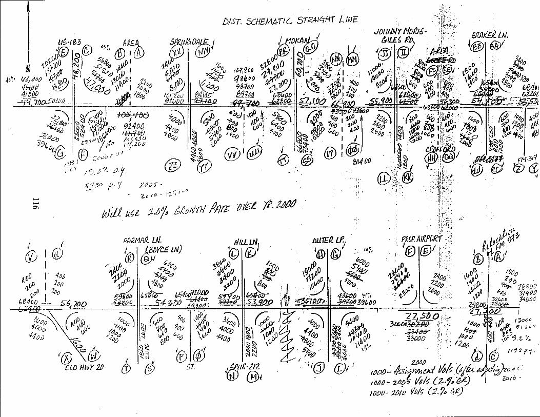
D/ST. 5:JI£MA-TIG STI2AIr::rHT LINE
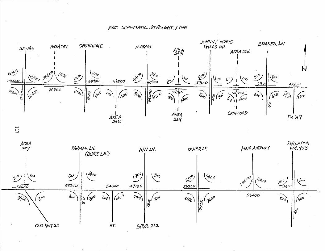
7/ 1ST. SCHE/'1A-Vc. .5t!J?ALr:dfLJ..Jtll3 •
JoHN N r MOR.IS 8R41<£R.. L.N
1 llS-t63 ARfA:2.S4 SfRlllfrPALE MorAN
AF$A GILfS RD.
AReA ;;1,11/.. , .:l~3
I I I I I I I J N I~J OJI ;;
~ ~. fJ'!J ~ ''z ~ ~ I ~. \t ~oo~l~ d~ ~o ~I't -4.~ . _. I I~~~oo b9500 ~()O S"J!>OO --L- 5"230') ;;1.'8..0 <"")
~~ r:? 1.5"900 ~ ~r:;:o I
~ ~(id: 5910--~ (j --B?oo ~ r;o~ ~ ~I~ o dJ it \\U! ~I~ ~Q;O ~I~ ti \ P;; J \5 " I 4aO 1\0
~ : I I , I A~A CKOfFOI<J)
R13'7 AREA ::uq .;lbB
~ ~ -.l
AR.PA Rf/.l;Ifirto JI ;2.2.7 PMM/tR LN. HILL 111. O()rERLP. /WP. AIRpoRf PM. 973 I (eoYCELN,)
I I
~ ~ V''t. ~ ~ ~ ~ :5 ~o ~ ~ -L ,'J.-\ :;;z6r:.r:, &3:2012 53-:200 54.600 47100 26'U;o ~- --
\ (;0 34 &W ~ !? ~ (;0 ~~ r,)r;;O 26400 ~ r:;; ~ ~ ~ ()
t ~
CiD HW'(:20 5" 5f1.!f<. 212
-.
APPENDIX B
Intersection Volumes Along US-290.
118

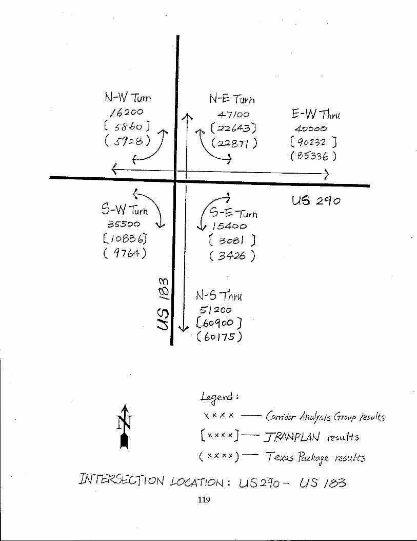
N-WTurn N-f; TUrh 16200
/ ~ 4-7/00 F-W/lwu >', .
(58~ ~b43) 40000
( .s-Cf:2 6 ) (22871 ) (qo2?;1- J ( B5'3'3b )
I , , /
U6 2'10 S-W~ S-rU'~ 35500 /5400 l/oBBb) ( 3051 J ( 1764) ( 3426 )
t'()
~ N-S 1hr~ --~
5"1 ::200
~~ (.6oqoo J (6 0 /75)
~Atl;
x )( x x - Com'dcr Ana!rsi:; Grot-1p jesu!ts
( )( x X x J - J7?ANPLAJJ te-:.ul1s
( )(. x x )C ) - T exa.s PackOJ~ r:?-50uJts
INTEt<.5£G{ION W("ATIO"-J = US 210 - US /83 119
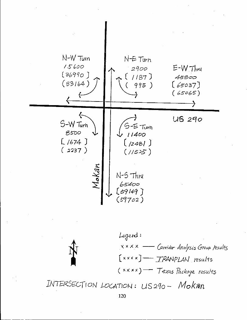
N-WTuyn /SbOO
(':3b9Cfo J ('33/~
I
s-w~ BSD~urh ~
l/674 J ( :2237 )
N-t:. Turh
/~ ·2Qoo
\ ~ / ~S7) ~75 )
~--rlJrh l ~~~OO (/2461 J (//5~S )
/-b?~rd !
S-WTlwu 4-5So:::>
( b5037J ( 6.50 65)
, /
US 2'10
X X X. x - (Pm'dor 4nafySi.5 Group ~sult.s
( x )()( x J - _Ti<ANPLAJJ . ~suliS
( x>< X 1. ) - Texa.s PackOJ~ r~s.{jJts
LN/~-rION WCATION = US210 - Mokan 120
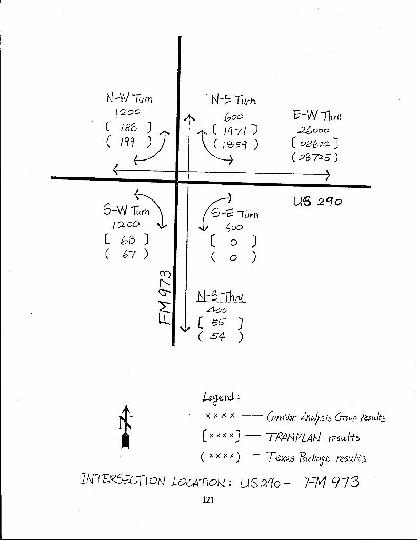
t-J-w Turn 1'200 ( !8:J;
( /~9 )
I ,
s-w~ I':). 00 .
l bB J ( 67 )
rr) f'.. <:!--
a:
N-&. Tu.rh
/ r" bOO S-VVThru \J.E7! ') .:2.{;,ooo
( 1<05"'1 ) ( 286'2.'2. J (.2272 5 )
, /
US 2Cfo 14IU'11 bOo
( 0 J ( 0 )
~S:ThH{ .- - ... _-400
,~ [ 55 ) . ( 54 )
~A-d;
x x x x - Com'dar Anaysi.5 Gror.Lp tesu/fS
( x )( )l x ] - TRANPLAIJ . t'e-:.ul1s
( )( >< X;l. ) - Texa.s PctckOJ.t r~~uJts
lNTEt<5£GiION WG,4.TION = US210 - PM 973 121

APPENDIX C
An Example of Turning Movements at SH-161.
122

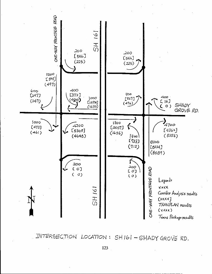
~ ~
~ i -::r: >-
~ 200 en ..200 \
[5«:>J ~ l54b] (.;225) (~ )t
I-u>O ( 5t>5J (4tJ7)
"00 400 '?ljJ !:)bO
(247J~ 1000 [;]7 4ao . (~O) ~bJ (1.47) C14Q4] (4%) ,~ (.0) SHADY ~ (143?)
&Rove R.D.
) IOOO~ 1=300 n 700
~ (473J a lOO (.2057J [-53b"l. J
(4'" ) (53b5J (1"56)
( 535 6) (4b4~)
('738J 6200 (712) [B234]
(~8~)
~ • .f?j ..:1.00 a ( 0) c. 0) ~ ( 0) ( 0) ~
~ Lea~dl ~)(,()(
\0 ~ Com'dol" AtqJ/SI'~ Ye.~.s -:r:: >- ()(XXX]
(f) ~ TRAN PL.AN ~~ts I
(')( xu.)
~ T~o.s f?,.d:c.r t£~
123

APPENDIX D
Turning Movement Iterative Procedure Using Lotus.
124

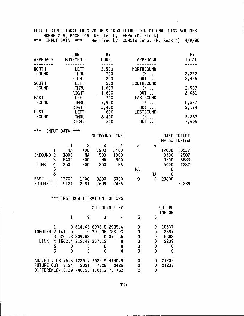
FUTURE DIRECTIONAL TURN VOLUMES FROM FUTURE DIRECTIONAL LINK VOLUMES NCHRP 255, PAGE 105 Written by: FHWA (C. Fleet)
*** INPUT DATA *** Modified by: COMSIS Corp. (M. Roskin) 4/9/86
TURN BY FY APPROACH MOVEMENT COUNT APPROACH TOTAL -------- -------- --------NORTH LEFT 3,500 NORTHBOUND
BOUND THRU 700 IN ... 2,232 RIGHT 800 OUT ... 2,425
SOUTH LEFT 500 SOUTHBOUND BOUND THRU 1,000 IN ... 2,587
RIGHT 1,800 OUT ... 2,081 EAST LEFT 700 EASTBOUND
BOUND THRU 7,900 IN ... 10,537 RIGHT 3,400 OUT ... 9,124
WEST LEFT 600 WESTBOUND BOUND THRU 8,400 IN 5,883
RIGHT 500 OUT ... 7,609
*** INPUT DATA *** OUTBOUND LINK BASE FUTURE
INFLOW INFLOW 1 2 3 4 5 6
1 NA 700 7900 3400 12000 10537 INBOUND 2 1800 NA 500 1000 3300 2587
3 8400 500 NA 600 9500 5883 LINK 4 3500 700 800 NA 5000 2232
5 NA a 6 NA a
BASE . 13700 1900 9200 5000 a a 29800 FUTURE 9124 2081 7609 2425 21239
***FIRST ROW ITERATION FOLLOWS
OUTBOUND LINK FUTURE INFLOW
1 2 3 4 5 6
1 a 614.65 6936.8 2985.4 a a 10537 INBOUND 2 1411. a a 391. 96 783.93 a a 2587
3 5201. 8 309.63 a 371.55 a a 5883 LINK 4 1562.4 312.48 357.12 a a a 2232
5 a a a a a a a 6 a a a a a a a
ADJ.FUT. 08175.3 1236.7 7685.9 4140.9 a a 21239 FUTURE OUT 9124 2081 7609 2425 a a 21239 DIFFERENCE-10.39 -40.56 1.0112 70.762 a a
125
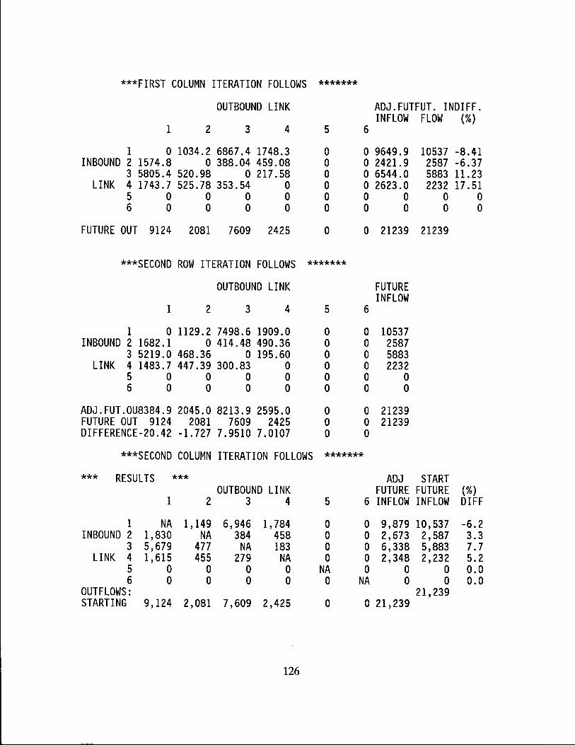
***FIRST COLUMN ITERATION FOLLOWS *******
OUTBOUND LINK ADJ. FUTFUT. INDIFF. INFLOW FLOW (%)
1 2 3 4 5 6
1 o 1034.2 6867.4 1748.3 0 o 9649.9 10537 -8.41 INBOUND 2 1574.8 o 388.04 459.08 0 o 2421. 9 2587 -6.37
3 5805.4 520.98 o 217.58 0 o 6544.0 5883 11. 23 LINK 4 1743.7 525.78 353.54 0 0 o 2623.0 2232 17.51
5 0 0 0 0 0 0 0 0 0 6 0 0 0 0 0 0 0 0 0
FUTURE OUT 9124 2081 7609 2425 0 0 21239 21239
***SECOND ROW ITERATION FOLLOWS *******
OUTBOUND LINK FUTURE INFLOW
1 2 3 4 5 6
1 o 1129.2 7498.6 1909.0 0 0 10537 INBOUND 2 1682.1 o 414.48 490.36 0 0 2587
3 5219.0 468.36 o 195.60 0 0 5883 LINK 4 1483.7 447.39 300.83 0 0 0 2232
5 0 0 0 0 0 0 0 6 0 0 0 0 0 0 0
ADJ.FUT.OU8384.9 2045.0 8213.9 2595.0 0 0 21239 FUTURE OUT 9124 2081 7609 2425 0 0 21239 DIFFERENCE-20.42 -1.727 7.9510 7.0107 0 0
***SECOND COLUMN ITERATION FOLLOWS *******
*** RESULTS *** ADJ START OUTBOUND LINK FUTURE FUTURE (%)
1 2 3 4 5 6 INFLOW INFLOW DIFF
1 NA 1,149 6,946 1,784 0 0 9,879 10,537 -6.2 INBOUND 2 1,830 NA 384 458 0 0 2,673 2,587 3.3
3 5,679 477 NA 183 0 0 6,338 5,883 7.7 LINK 4 1,615 455 279 NA 0 0 2,348 2,232 5.2
5 0 0 0 0 NA 0 0 0 0.0 6 0 0 0 0 0 NA 0 0 0.0
OUTFLOWS: 21,239 STARTING 9,124 2,081 7,609 2,425 0 o 21,239
126
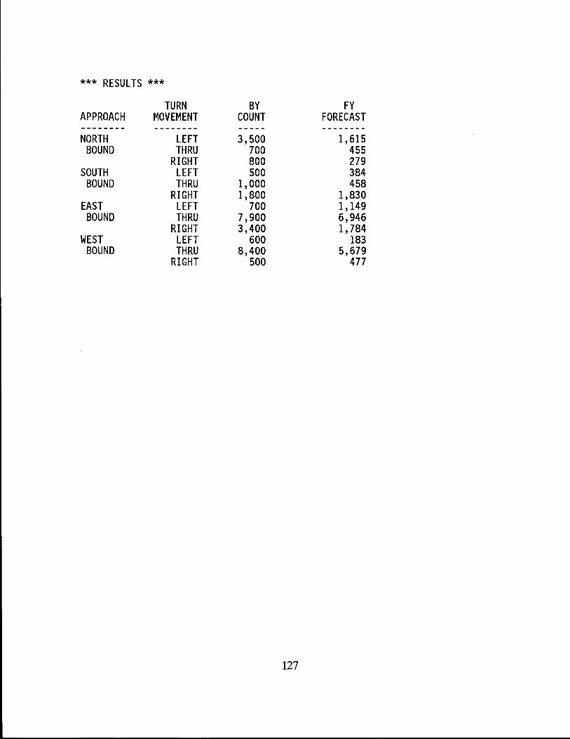
*** RESULTS ***
TURN BY FY APPROACH MOVEMENT COUNT FORECAST -------- -------- --------NORTH LEFT 3,500 1,615
BOUND THRU 700 455 RIGHT 800 279
SOUTH LEFT 500 384 BOUND THRU 1,000 458
RIGHT 1,800 1,830 EAST LEFT 700 1,149
BOUND THRU 7,900 6,946 RIGHT 3,400 1,784
WEST LEFT 600 183 BOUND THRU 8,400 5,679
RIGHT 500 477
127

APPENDIX E
Turning Movement Procedures.
This appendix is a condensation of Chapter 8 of the User's Guide contained in NCHRP
Report 255.
128

Introduction
Scope
Turning movement data are often required for the planning and design of highway intersections and interchanges. Therefore, procedures have been developed to enable the analyst to develop these data from sources and various uses. This appendix summarizes the procedures documented in "Highway Traffic Data For Urbanized Area Project Planning and Design," NCHRP Report 255, pp. 102-114.
Example problems to illustrate the five calculations involved are included at the end of this appendix.
The methodologies covered are as follows:
* * * * * *
*
Factoring procedure Iterative procedure Directional volume method of iterative procedure Nondirectional volume method of iterative procedure "T" intersection procedure Directional turning movement method of "T" intersection procedure Nondirectional turning movement method of "T" intersection procedure
129
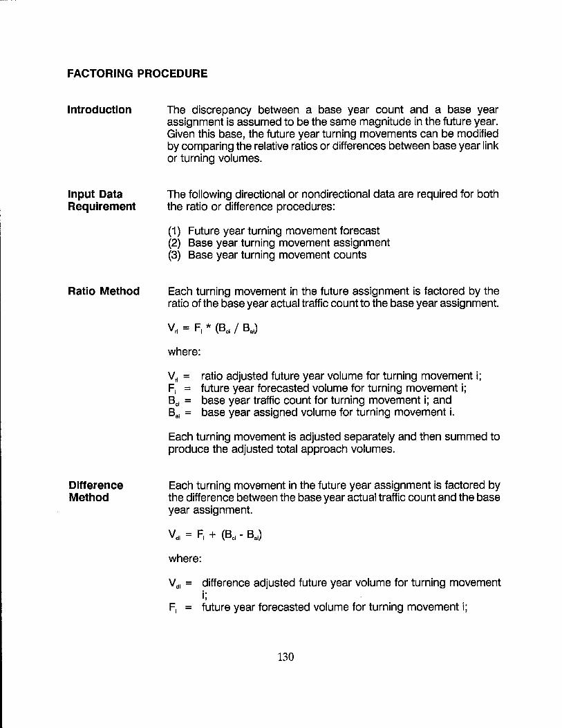
----------- -------- -----
FACTORING PROCEDURE
Introduction
Input Data Requirement
Ratio Method
Difference Method
The discrepancy between a base year count and a base year assignment is assumed to be the same magnitude in the future year. Given this base, the future year turning movements can be modified by comparing the relative ratios or differences between base year link or turning volumes.
The following directional or nondirectional data are required for both the ratio or difference procedures:
(1) Future year turning movement forecast (2) Base year turning movement assignment (3) Base year turning movement counts
Each turning movement in the future assignment is factored by the ratio of the base year actual traffic count to the base year assignment.
where:
Vrl = ratio adjusted future year volume for turning movement i; F, = future year forecasted volume for turning movement i; Bc' = base year traffic count for turning movement i; and Sal = base year assigned volume for turning movement i.
Each turning movement is adjusted separately and then summed to produce the adjusted total approach volumes.
Each turning movement in the future year assignment is factored by the difference between the base year actual traffic count and the base year assignment.
where:
Vdl = difference adjusted future year volume for turning movement i;
F, = future year forecasted volume for turning movement i;
130
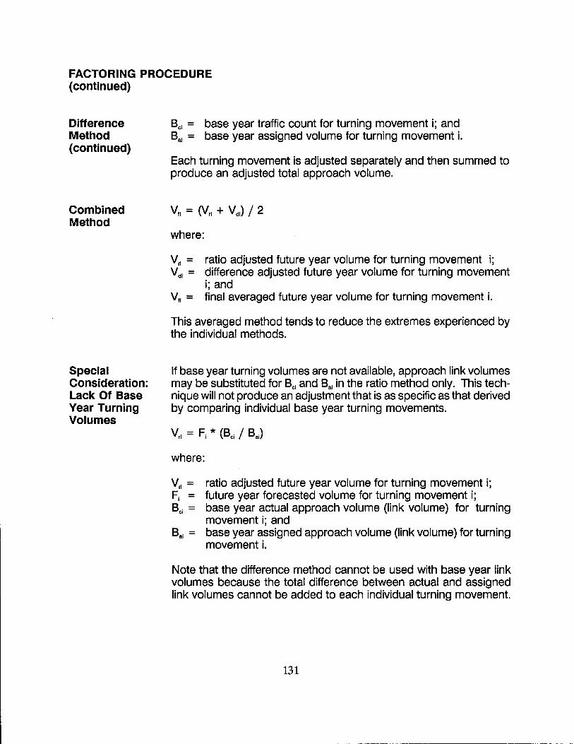
FACTORING PROCEDURE (continued)
Difference Method (continued)
Combined Method
Special Consideration: Lack Of Base Year Turning Volumes
BCI = base year traffic count for turning movement i; and Bal = base year assigned volume for turning movement i.
Each turning movement is adjusted separately and then summed to produce an adjusted total approach volume.
where:
V'I = ratio adjusted future year volume for turning movement i; Vdl = difference adjusted future year volume for turning movement
i; and VII = final averaged future year volume for turning movement i.
This averaged method tends to reduce the extremes experienced by the individual methods.
If base year turning volumes are not available, approach link volumes may be substituted for BCI and Bal in the ratio method only. This technique will not produce an adjustment that is as specific as that derived by comparing individual base year turning movements.
where:
V'I = ratio adjusted future year volume for turning movement i; F; = future year forecasted volume for turning movement i; Bc; = base year actual approach volume (link volume) for turning
movement i; and Bal = base year assigned approach volume (link volume) for turning
movement i.
Note that the difference method cannot be used with base year link volumes because the total difference between actual and assigned link volumes cannot be added to each individual turning movement.
131
DIRECTIONAL VOLUME METHOD OF ITERATIVE PROCEDURE
Introduction
Input Data Requirement
Directions for Use
The directional volume method proceeds through an iterative computational technique to produce a final set of future year turning volumes. The computations involve alternatively balancing the rows (inflows) and columns (outflows) of a turning movement matrix until an acceptable convergence is obtained. Normally, a maximum of six to ten iterations requiring one or two person-hours should suffice.
The following input data are required:
* *
Future year directional link volumes Either base year actual or assigned directional turning movements; initial estimate of future year directional turning movements.
The base year data preferably would be actual turning movement counts, but turning data from a base year assignment could also be used. In lieu of base year data, the analyst must make an initial estimate of future year turning percentages based on an examination of adjacent land uses or the turning movements at similar intersections.
The directional volume method consists of five steps, and the following notations are used in the calculations:
n = number of links emanating from the intersection; Olb = base year (b) inflow to the intersection on link i; Olf = future year (f) inflow to the intersection on link i; Djb = base year (b) outflow from the intersection on link j; Djf = future year (f) outflow from the intersection on link j; Tjjb = base year (b) traffic flow entering through link i and leaving link
j; Tjjf = future year (f) traffic flow entering through link i and leaving link
j; Pljf = future year (f) estimated percentage of traffic flow from link i to
link j; and * = adjusted values in each iteration.
132
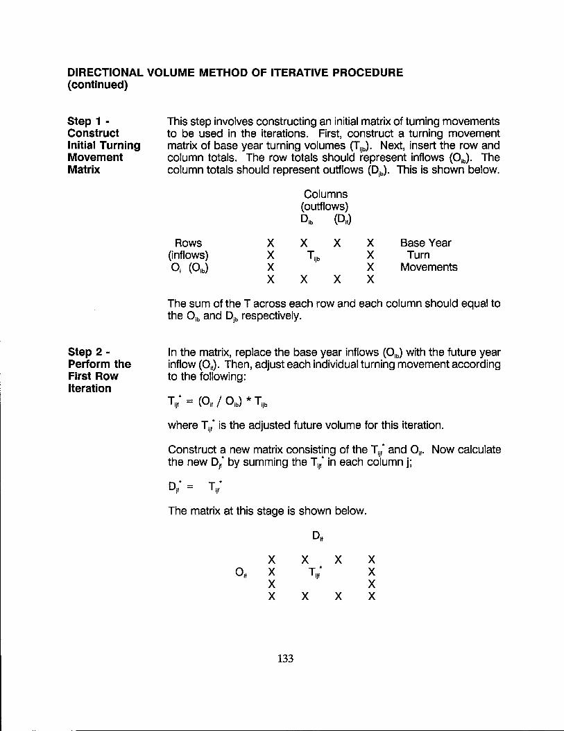
DIRECTIONAL VOLUME METHOD OF ITERATIVE PROCEDURE (continued)
Step 1 -Construct Initial Turning Movement Matrix
Step 2-Perform the First Row Iteration
This step involves constructing an initial matrix of turning movements to be used in the iterations. First, construct a turning movement matrix of base year turning volumes (TIJb)' Next, insert the row and column totals. The row totals should represent inflows (Olb)' The column totals should represent outflows (DJb). This is shown below.
Columns (outflows) Dlb (Dw)
Rows X X X X Base Year (inflows) X TIJb X Turn 0 1 (Olb) X X Movements
X X X X
The sum of the T across each row and each column should equal to the 0lb and DJb respectively.
In the matrix, replace the base year inflows (Olb) with the future year inflow (Olf)' Then, adjust each individual turning movement according to the following:
Tlj; = (Olf / Olb) * TIJb
where TIJ; is the adjusted future volume for this iteration.
Construct a new matrix consisting of the Tlj; and 0lf' Now calculate the new DJ; by summing the TIJ; in each column j;
The matrix at this stage is shown below.
X X X X
133
X X
X X X X
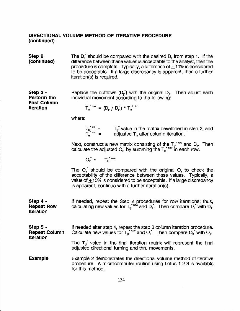
DIRECTIONAL VOLUME METHOD OF ITERATIVE PROCEDURE (continued)
Step 2 (continued)
Step 3-Perform the First Column Iteration
Step 4-Repeat Row Iteration
Step 5 -Repeat Column Iteration
Example
The D/ should be compared with the desired DJf from step 1. If the difference between these values is acceptable to the analyst, then the procedure is complete. Typically, a difference of ± 10% is considered to be acceptable. If a large discrepancy is apparent, then a further iteration(s) is required.
Replace the outflows (Djf") with the original Djf. Then adjust each individual movement according to the following:
where:
T "new - (D / D ") * T "old ijf - jf Jf ijf
T "old -ijf -T • new -
Ijf -TIJf" value in the matrix developed in step 2, and adjusted Tijf after column iteration.
Next, construct a new matrix consisting of the Tijf" new and Djf" Then calculate the adjusted Olf" by summing the TIJf" new in each row.
T * new IJf
The Olf" should be compared with the original Olf to check the acceptability of the difference between these values. Typically, a value of ± 10% is considered to be acceptable. If a large discrepancy is apparent, continue with a further iteration(s).
If needed, repeat the Step 2 procedures for row iterations; thus, calculating new values for Tljf" new and Djf". Then compare DJf" with Djf"
If needed after step 4, repeat the step 3 column iteration procedure. Calculate new values for TiJf" new and o If" • Then compare Olf" with OJ("
The TIJf" value in the final iteration matrix will represent the final adjusted directional turning and thru movements.
Example 2 demonstrates the directional volume method of iterative procedure. A microcomputer routine using Lotus 1-2-3 is available for this method.
134
NON DIRECTIONAL VOLUME METHOD OF ITERATIVE PROCEDURE
Introduction
Input Data Requirement
Directions for Use
Step 1 -Estimate Total Turning Percentage
Step 2 -Calculate the Relative Weight of Each Intersection Approach
The nondirectional volume method produces two-way turning volumes and an estimate of the total vehicle turning percentage. Turning movements at an intersection should be some function of the attractions and productions each direction of travel offers.
The method provides a five-step sequence and may have to be performed iteratively to achieve a balanced distribution of turning and thru movements. The number of iterations will vary, but three to four iterations requiring one to three person-hours will be sufficient.
Nondirectional link volumes (Le., total both directions) on each approach are required input data for this method.
The five-step methodology for the nondirectional volume method is described below.
The first step is to determine the percentage of total inflowing traffic which turns (either right or left). The turning percentage value must normally be estimated based on the unique characteristics of the intersection and comparable intersections from other parts of the urban area.
If the actual signal green times given to individual turning movements are known at the subject intersection, these values can be used instead of the estimated percentage for the entire intersection.
This turning movement percentage is estimated relative to the sum of only inflowing (Le., one direction) volume. The inflowing volume equals one-half of the total nondirectional volume.
Calculate the relative weight of each intersection approach. Sum all nondirectional volumes on all the intersection approaches. Express the volume on a particular approach as a proportion of total volume. The proportions (or relative weight) on all approaches must sum to 1.00.
135
----~---~ ---------------------
NONDIRECTIONAL VOLUME METHOD OF ITERATIVE PROCEDURE (continued)
Step 3 -Perform Initial Allocation of Turns
Step 4-Adjust Turning Volumes Based on Turning Percentage
Step 5-Balance the Approach Volumes and Adjusted Turning Volumes
This step involves allocating the volume in each approach to the other intersection approaches. Multiply the total volume on an approach by the relative weights, as computed in Step 2 for the remaining approaches which involve turns. This calculation should be performed for each intersection approach to produce turns to the other approaches.
The total volume of turns generated in Step 3 will typically exceed the likely volume of turns at the intersection. To adjust the step 3 estimates, a turning adjustment needs to be imposed. The adjustment involves the following computations:
(a) Write down the total inflowing volume (Step 1) (b) Write down the total turn percentage (step 2) (c) Compute total expected volume of turns as (a) x (b) (d) Sum the turning volume calculated during Step 3 (e) Adjust the individual turns from Step 3 using either a difference
method or ratio method
Difference method: Va = (Ve - Vd) / 4 Ratio method: Re = Ve / Vd
where:
Va = volume to be subtracted from each turning volume Ve = turning volume from Step 4(c) Vd = turning volume from Step 4(d) Ra = ratio to be multiplied by each turning volume.
At the end of this step, the total volume of turns at the intersection will be equal to the expected volume total from Step 1.
Typically the preceding steps will yield a turning movement estimate that conforms to the estimated turning percentage established in Step 1. However, it is possible, even likely, that the method will not yield an intersection scenario that accounts for all the traffic traversing the intersection.
To test for this situation, take each approach of the intersection and do the following:
136
NONDIRECTIONAL VOLUME METHOD OF ITERATIVE PROCEDURE (continued)
Step 5 (continued)
(a) Write down the total approach volume (b) Subtract the turns made to/from that approach from cross
streets (c) Add the turns made to/from the approach on the opposite side
of the intersection
If the intersection clears all traffic, the total volume on the opposing approach of the intersection should equal the volume estimated from the above test. If these volumes do not correspond, out-of-balance numbers need to be adjusted to bring the analysis into equilibrium.
Two situations are normally encountered in this analysis:
(a) The opposite intersection approaches show a greater difference in adjusted volume (Step 5) than was evident in the original volumes (Step 2).
(b) The two opposing intersection approaches having adjusted volumes (Step 5) are closer to each other than was evident in the original volume (Step 2).
In the first situation, iterating the entire procedure from Step 2 using the new approach volumes will narrow the volume difference between two opposing intersection approaches.
The second situation in which the differences in volume on opposing approaches needs to be increased is more complicated. The following computations will provide an adjustment which will increase the difference between the opposing volumes.
(a) Sum the volumes on the two opposing approaches using the original volumes input at the outset of the analysis (Step 2).
(b) Determine the proportion of this volume (a) represented by each of the two opposing approaches. This must sum up to 1.00.
(c) Determine the approach volume difference between the adjusted and the original estimates.
(d) Multiply the proportions (b) by the volume difference (c). Add/subtract this number to/from the calculated volumes as appropriate.
137
NONDIRECTIONAL VOLUME METHOD OF ITERATIVE PROCEDURE (continued)
Step 5 (continued)
Example
The above adjustments should be applied to each intersection approach in order to insure that the approach volumes are in scale relative to the completed turning volumes.
Example 3 demonstrates the nondirectional volume method of iterative procedure. A microcomputer routine using Lotus 1-2-3 is available for this method.
138
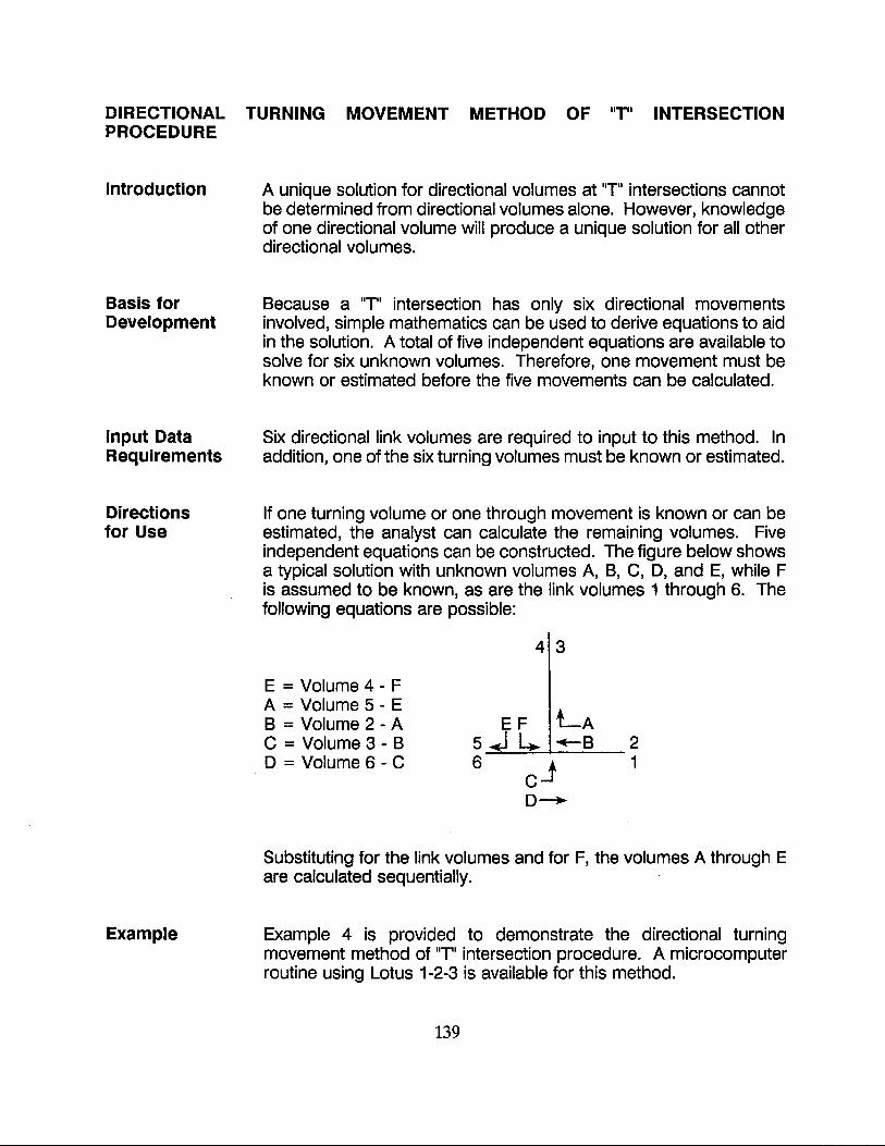
DIRECTIONAL TURNING MOVEMENT METHOD OF "r' INTERSECTION PROCEDURE
Introduction
Basis for Development
Input Data Requirements
Directions for Use
Example
A unique solution for directional volumes at 'T' intersection.s cannot be determined from directional volumes alone. However, knowledge of one directional volume will produce a unique solution for all other directional volumes.
Because a "T" intersection has only six directional movements involved, simple mathematics can be used to derive equations to aid in the solution. A total of five independent equations are available to solve for six unknown volumes. Therefore, one movement must be known or estimated before the five movements can be calculated.
Six directional link volumes are required to input to this method. In addition, one of the six turning volumes must be known or estimated.
If one turning volume or one through movement is known or can be estimated, the analyst can calculate the remaining volumes. Five independent equations can be constructed. The figure below shows a typical solution with unknown volumes A, B, C, D, and E, while F is assumed to be known, as are the link volumes 1 through 6. The following equations are possible:
E = Volume 4 - F A = Volume 5 - E B = Volume 2 - A C = Volume 3 - B D = Volume 6 - C
4 3
2 1
Substituting for the link volumes and for F, the volumes A through E are calculated sequentially.
Example 4 is provided to demonstrate the directional turning movement method of "T" intersection procedure. A microcomputer routine using Lotus 1-2-3 is available for this method.
139
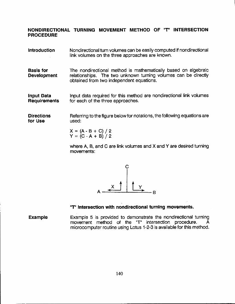
NONDIRECTIONAL TURNING MOVEMENT METHOD OF "T" INTERSECTION PROCEDURE
Introduction
Basis for Development
Input Data Requirements
Directions for Use
Example
Nondirectional turn volumes can be easily computed if nondirectional link volumes on the three approaches are known.
The nondirectional method is mathematically based on algebraic relationships. The two unknown turning volumes can be directly obtained from two independent equations.
Input data required for this method are nondirectional link volumes for each of the three approaches.
Referring to the figure below for notations, the following equations are used:
x = (A - B + C) / 2 Y = (C - A + B) / 2
where A, B, and C are link volumes and X and Yare desired turning movements:
C
L1~ A---'----"'---~-B
"T" intersection with nondirectional turning movements.
Example 5 is provided to demonstrate the nondirectional turning movement method of the liT" intersection procedure. A microcomputer routine using Lotus 1-2-3 is available for this method.
140
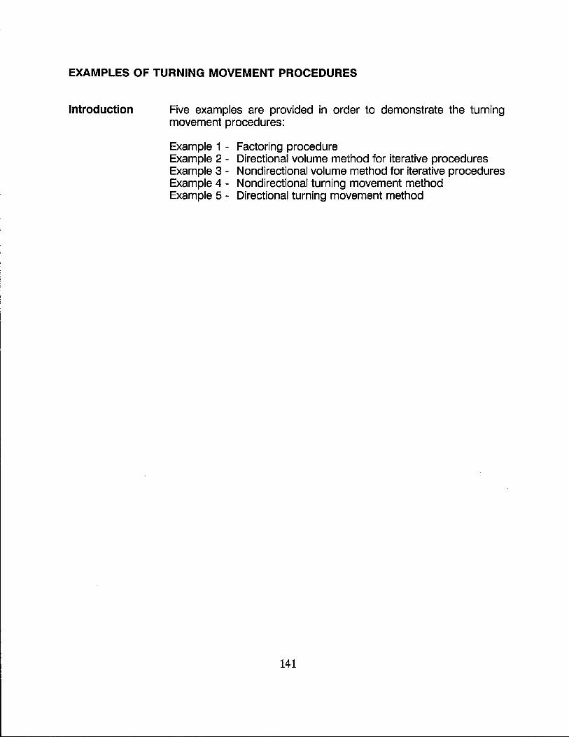
EXAMPLES OF TURNING MOVEMENT PROCEDURES
Introduction Five examples are provided in order to demonstrate the turning movement procedures:
Example 1 - Factoring procedure Example 2 - Directional volume method for iterative procedures Example 3 - Nondirectional volume method for iterative procedures Example 4 - Nondirectional turning movement method Example 5 - Directional turning movement method
141
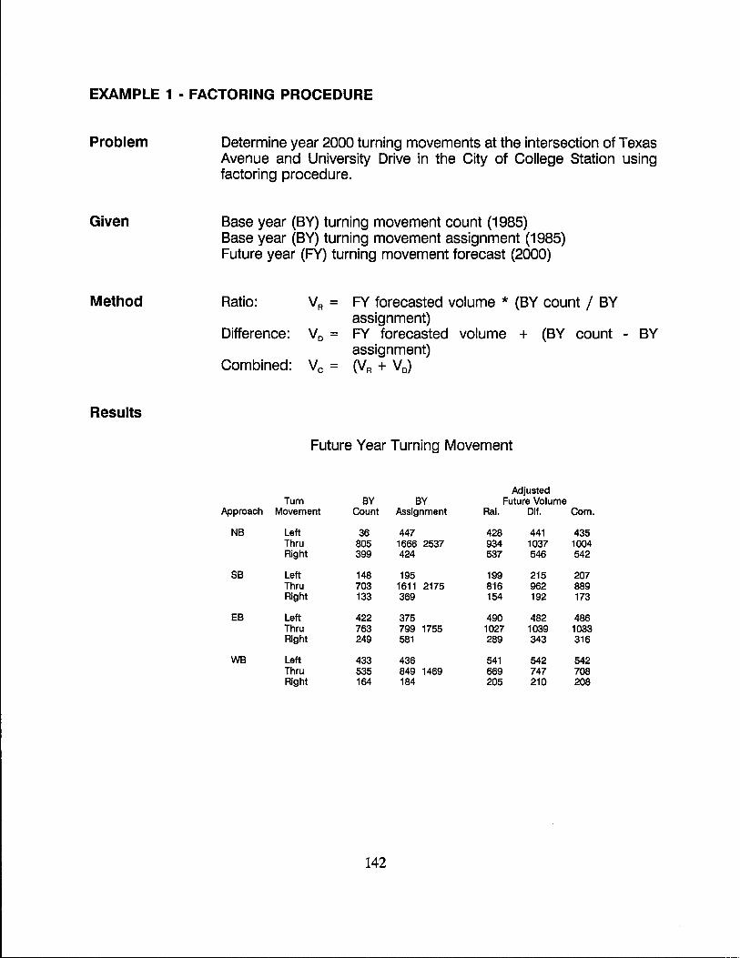
EXAMPLE 1 - FACTORING PROCEDURE
Problem
Given
Method
Results
Determine year 2000 turning movements at the intersection of Texas Avenue and University Drive in the City of College Station using factoring procedure.
Base year (BY) turning movement count (1985) Base year (BY) turning movement assignment (1985) Future year (FY) turning movement forecast (2000)
Ratio: VR = FY forecasted volume * (BY count / BY assignment)
Difference: VD = FY forecasted volume + (BY count -assignment)
Combined: Vc = (VR + VD)
Future Year Turning Movement
Adjusted Turn BY BY Future Volume
Approach Movement Count Assignment Rai. Dif. Com.
NB Left 36 447 428 441 435 Thru 805 1666 2537 934 1037 1004 Right 399 424 537 546 542
SB Left 148 195 199 215 207 Thru 703 1611 2175 816 962 889 Right 133 369 154 192 173
EB Left 422 375 490 482 486 Thru 763 799 1755 1027 1039 1033 Right 249 581 289 343 316
WB Left 433 436 541 542 542 Thru 535 849 1469 669 747 708 Right 164 184 205 210 208
142
BY
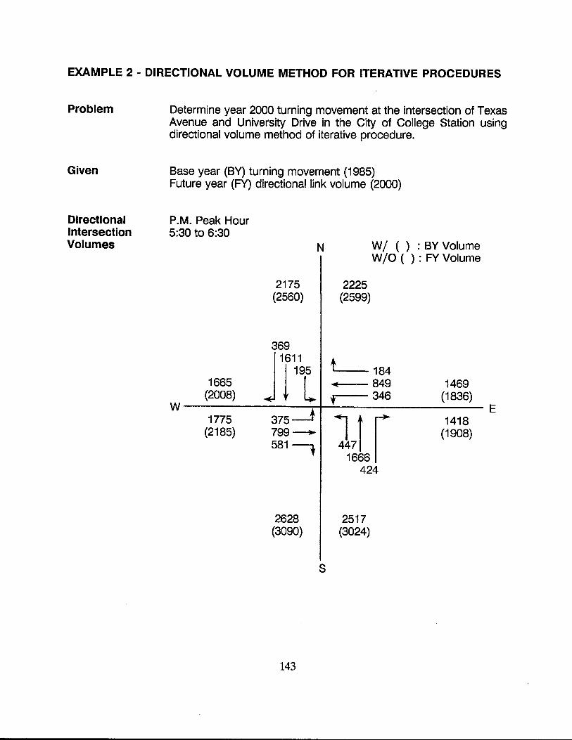
EXAMPLE 2 - DIRECTIONAL VOLUME METHOD FOR ITERATIVE PROCEDURES
Problem
Given
Directional Intersection Volumes
Determine year 2000 turning movement at the intersection of Texas Avenue and University Drive in the City of College Station using directional volume method of iterative procedure.
Base year (BY) turning movement (1985) Future year (FY) directional link volume (2000)
P.M. Peak Hour 5:30 to 6:30
1665 (2008)
W 1775
(2185)
N
2175 2225 (2560) (2599)
369
JTt t IIIIE
f
WI ( ) : BY Volume W/O ( ) : FY Volume
184 849 1469 346 (1836)
375---1
~~tr 1418
799 ---. (1908) 581 f
424
2628 2517 (3090) (3024)
S
143
E
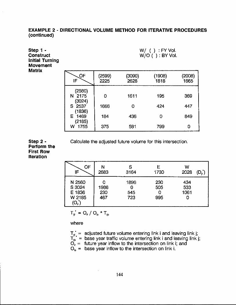
EXAMPLE 2 - DIRECTIONAL VOLUME METHOD FOR ITERATIVE PROCEDURES (continued)
Step 1 -Construct Initial Turning Movement Matrix
Step 2 -Perform the First Row Iteration
~ (2599) IF 2225
(2560) N 2175 0
(3024) S 2537 1666
(1836) E 1469 184
(2185) W 1755 375
(3090) 2628
1611
0
436
581
WI ( ) : FY Vol. WIO ( ) : BY Vol.
(1908) 1818
195
424
0
799
(2008) 1665
369
447
849
0
Calculate the adjusted future volume for this intersection.
~ N S E W IF 2683 3164 1730 2028
N 2560 0 1896 230 434 S 3024 1986 0 505 533 E 1836 230 545 0 1061 W 2185 467 723 995 0 (Oif")
where
(Dj;)
Tlj; = adjusted future volume entering link i and leaving link j; Tljb" = base year traffic volume entering link i and leaving link j; Oif = future year inflow to the intersection on link i; and Olb = base year inflow to the intersection on link i.
144
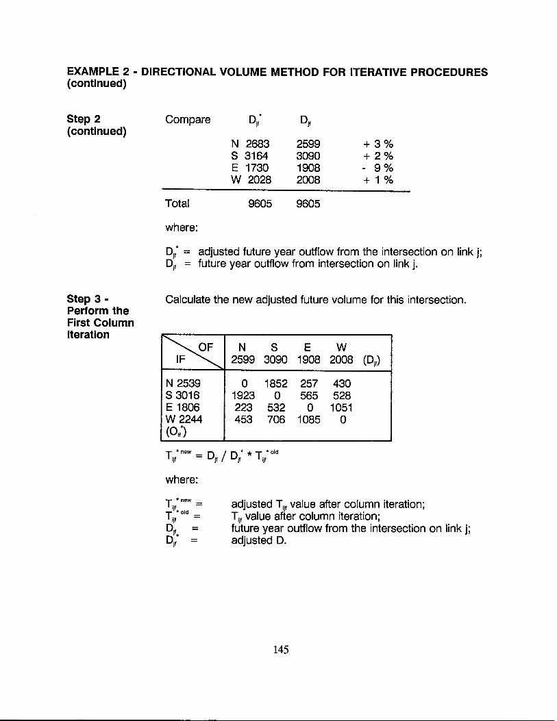
EXAMPLE 2 - DIRECTIONAL VOLUME METHOD FOR ITERATIVE PROCEDURES (continued)
Step 2 (continued)
Step 3-Perform the First Column Iteration
Compare Dj; Djf
N 2683 2599 + 3% S 3164 3090 + 2% E 1730 1908 - 9 % W 2028 2008 + 1 %
Total 9605 9605
where:
Djf* = adjusted future year outflow from the intersection on link j; Djf = future year outflow from intersection on link j.
Calculate the new adjusted future volume for this intersection.
~ N S E W IF 2599 3090 1908 2008 (Djf)
N 2539 0 1852 257 430 S 3016 1923 0 565 528 E 1806 223 532 0 1051 W2244 453 706 1085 0 (0;;)
T*new= D /D**T*old Ijf jf jf ;jf
where:
T. 1\' new =
T,jf*old _ Ijf -
Djf = Djf* =
adjusted Tijf value after column iteration; Tljf value after column iteration; future year outflow from the intersection on link j; adjusted D.
145
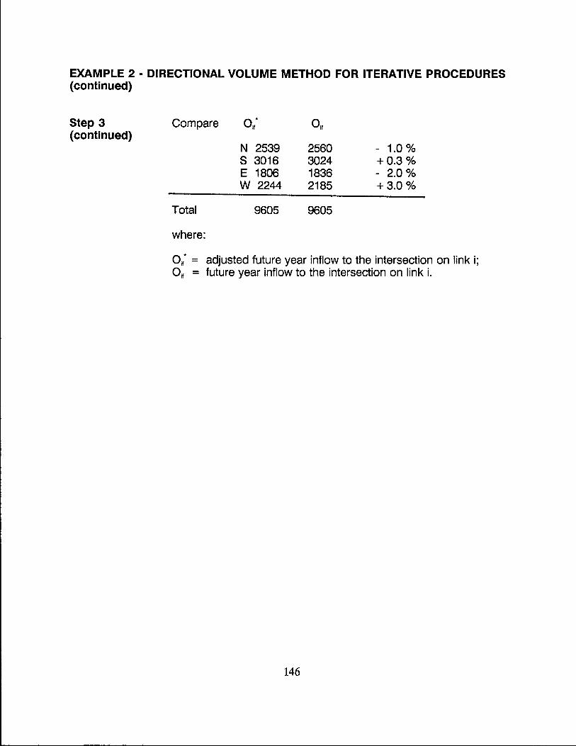
EXAMPLE 2 - DIRECTIONAL VOLUME METHOD FOR ITERATIVE PROCEDURES (continued)
Step 3 (continued)
Compare 0 1; O~
N 2539 2560 - 1.0 % S 3016 3024 +0.3% E 1806 1836 - 2.0 % W 2244 2185 +3.0%
Total 9605 9605
where:
Olf* = adjusted future year inflow to the intersection on link i; 0if = future year inflow to the intersection on link i.
146
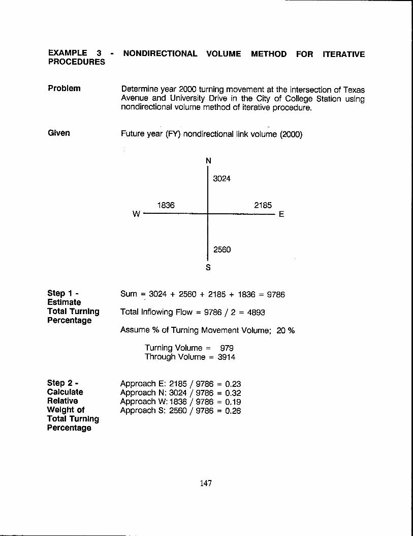
EXAMPLE 3 - NONDIRECTIONAL VOLUME METHOD FOR ITERATIVE PROCEDURES
Problem
Given
Step 1 -Estimate Total Turning Percentage
Step 2 -Calculate Relative Weight of Total Turning Percentage
Determine year 2000 turning movement at the intersection of Texas Avenue and University Drive in the City of College Station using nondirectional volume method of iterative procedure.
Future year (FY) nondirectional link volume (2000)
N
3024
1836 2185 W--------I------E
2560
S
Sum = 3024 + 2560 + 2185 + 1836 = 9786
Totallnflowing Flow = 9786/2 = 4893
Assume % of Turning Movement Volume; 20 %
Turning Volume = 979 Through Volume = 3914
Approach E: 2185 / 9786 = 0.23 Approach N: 3024 / 9786 = 0.32 Approach W: 1836/9786 = 0.19 Approach S: 2560/9786 = 0.26
147
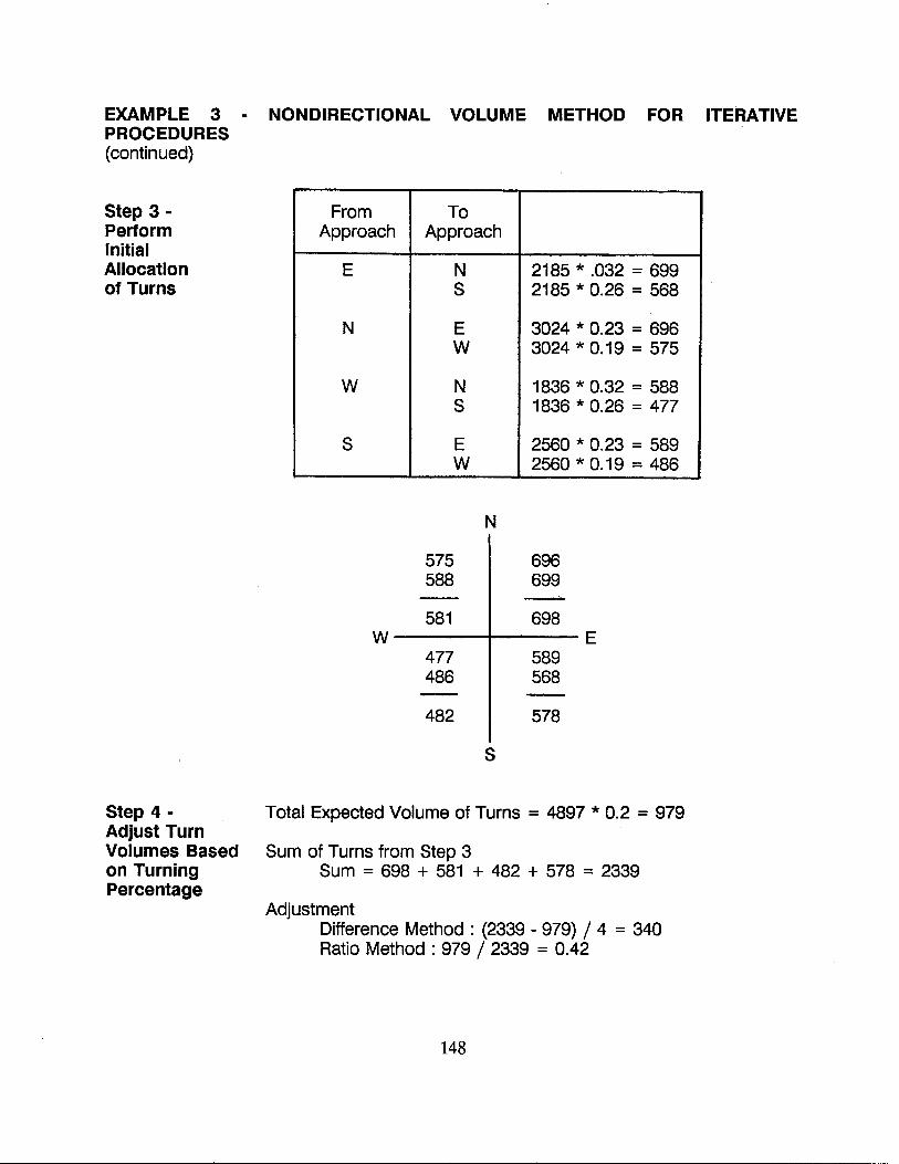
EXAMPLE 3 - NONDIRECTIONAL VOLUME METHOD FOR ITERATIVE PROCEDURES (continued)
Step 3 -Perform Initial Allocation of Turns
From To Approach Approach
E N 2185 * .032 = 699 S 2185 * 0.26 = 568
N E 3024 * 0.23 = 696 W 3024 * 0.19 = 575
W N 1836 * 0.32 = 588 S 1836 * 0.26 = 477
S E 2560 * 0.23 = 589 W 2560 * 0.19 = 486
N
575 696 588 699
581 698 W ----1---- E
477 486
482
s
589 568
578
Step 4 - Total Expected Volume of Turns = 4897 * 0.2 = 979 Adjust Turn Volumes Based Sum of Turns from Step 3 on Turning Sum = 698 + 581 + 482 + 578 = 2339 Percentage
Adjustment Difference Method : (2339 - 979) / 4 = 340 Ratio Method : 979 / 2339 = 0.42
148
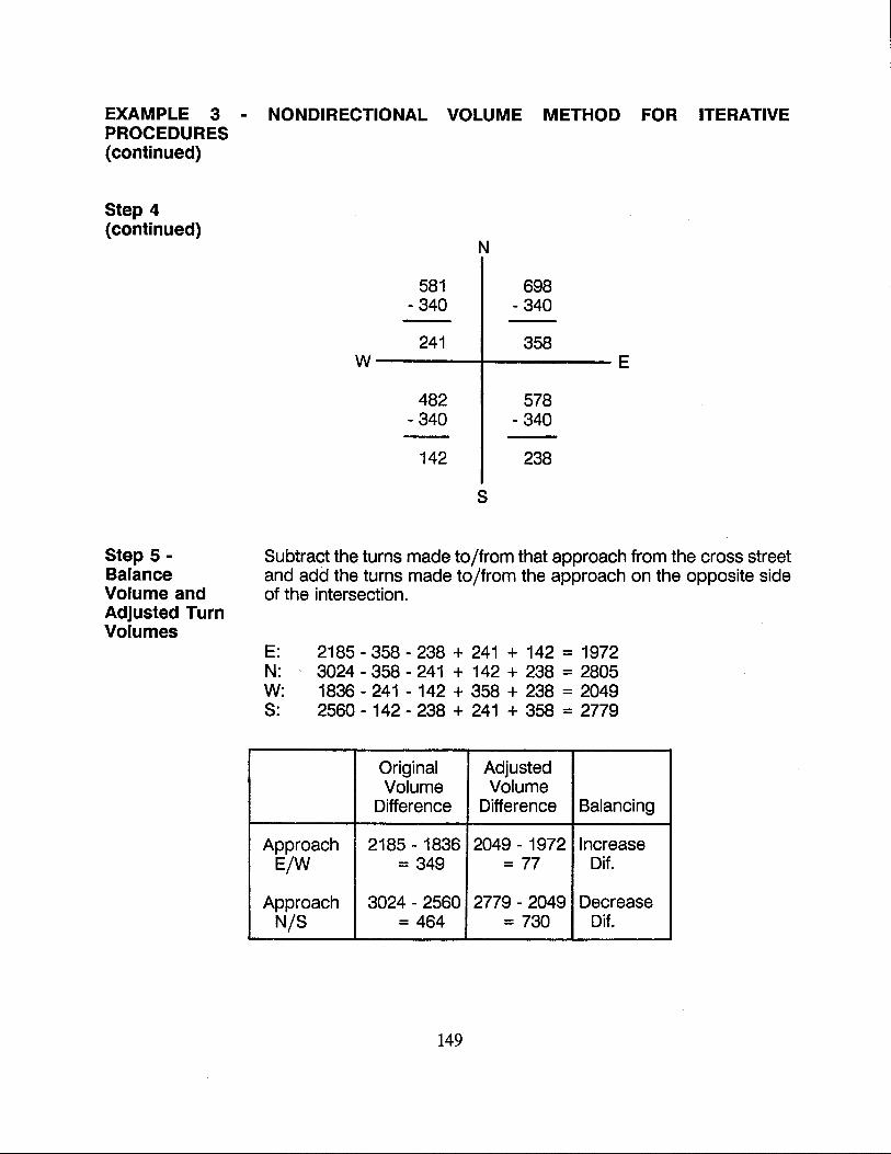
EXAMPLE 3 - NONDIRECTIONAL VOLUME METHOD FOR ITERATIVE PROCEDURES (continued)
Step 4 (continued)
Step 5-Balance Volume and Adjusted Turn Volumes
581 - 340
241
N
698 - 340
358 W -----+------ E
482 - 340
142
S
578 - 340
238
Subtract the turns made to/from that approach from the cross street and add the turns made to/from the approach on the opposite side of the intersection.
E: 2185 - 358 - 238 + 241 + 142 = 1972 N: 3024 - 358 - 241 + 142 + 238 = 2805 W: 1836 - 241 - 142 + 358 + 238 = 2049 S: 2560 - 142 - 238 + 241 + 358 = 2779
Original Adjusted Volume Volume
Difference Difference Balancing
Approach 2185 - 1836 2049 - 1972 Increase E/W = 349 = 77 Dif.
Approach 3024 - 2560 2779 - 2049 Decrease N/S = 464 = 730 Dif.
149
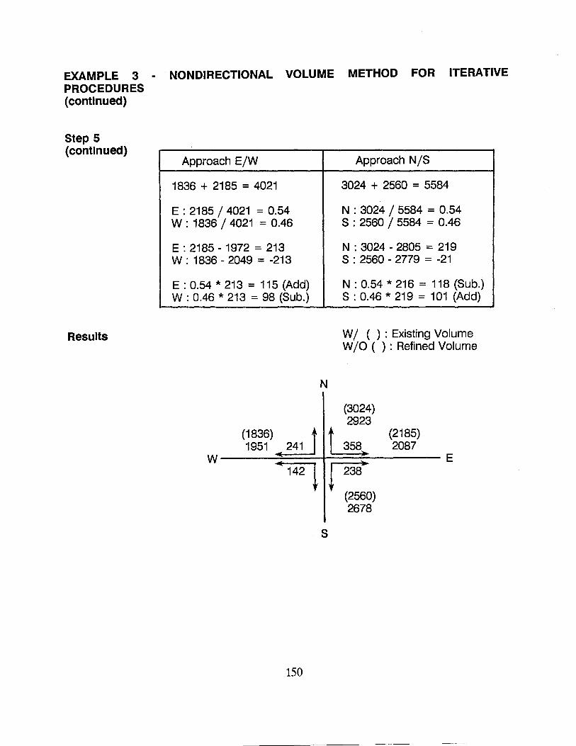
EXAMPLE 3 - NONDIRECTIONAL VOLUME METHOD FOR ITERATIVE PROCEDURES (continued)
Step 5 (continued)
Results
Approach E/W
1836 + 2185 = 4021
E : 2185/4021 = 0.54 W : 1836 / 4021 = 0.46
E : 2185 - 1972 = 213 W : 1836 - 2049 = -213
E : 0.54 * 213 = 115 (Add) W : 0.46 * 213 = 98 (Sub.)
N
Approach N/S
3024 + 2560 = 5584
N : 3024 / 5584 = 0.54 S : 2560/5584 = 0.46
N : 3024 - 2805 = 219 S : 2560 - 2779 = -21
N : 0.54 * 216 = 118 (Sub.) S : 0.46 * 219 = 101 (Add)
W / ( ) : Existing Volume W /0 ( ) : Refined Volume
(3024) 2923
(2185) 2087
(1836) _ .. t t 1951~ ~
W----=;;;;;;;;;;;;;;;;;,;;;;;;;;.~;;;;;;;;;;;;;;;;;;:;::;;;::;~---- E
~F (2560) 2678
S
150
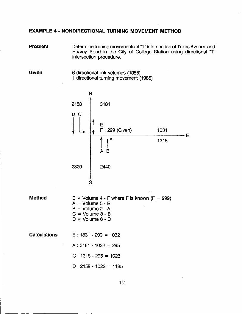
EXAMPLE 4 - NON DIRECTIONAL TURNING MOVEMENT METHOD
Problem
Given
Method
Calculations
Determine turning movements at liT" intersection of Texas Avenue and Harvey Road in the City of College Station using directional liT" intersection procedure.
6 directional link volumes (1985) 1 directional turning movement (1985)
N
2158 3181
D C
LE 1331 rF : 299 (Given)
~----------------------------E
t r 1 L
1318
A B
2320 2440
S
E = Volume 4 - F where F is known (F = 299) A = Volume 5 - E B = Volume 2 - A C = Volume 3 - B D = Volume 6 - C
E : 1331 - 299 = 1032
A : 3181 - 1032 = 295
C : 1318 - 295 = 1023
D: 2158 - 1023 = 1135
151
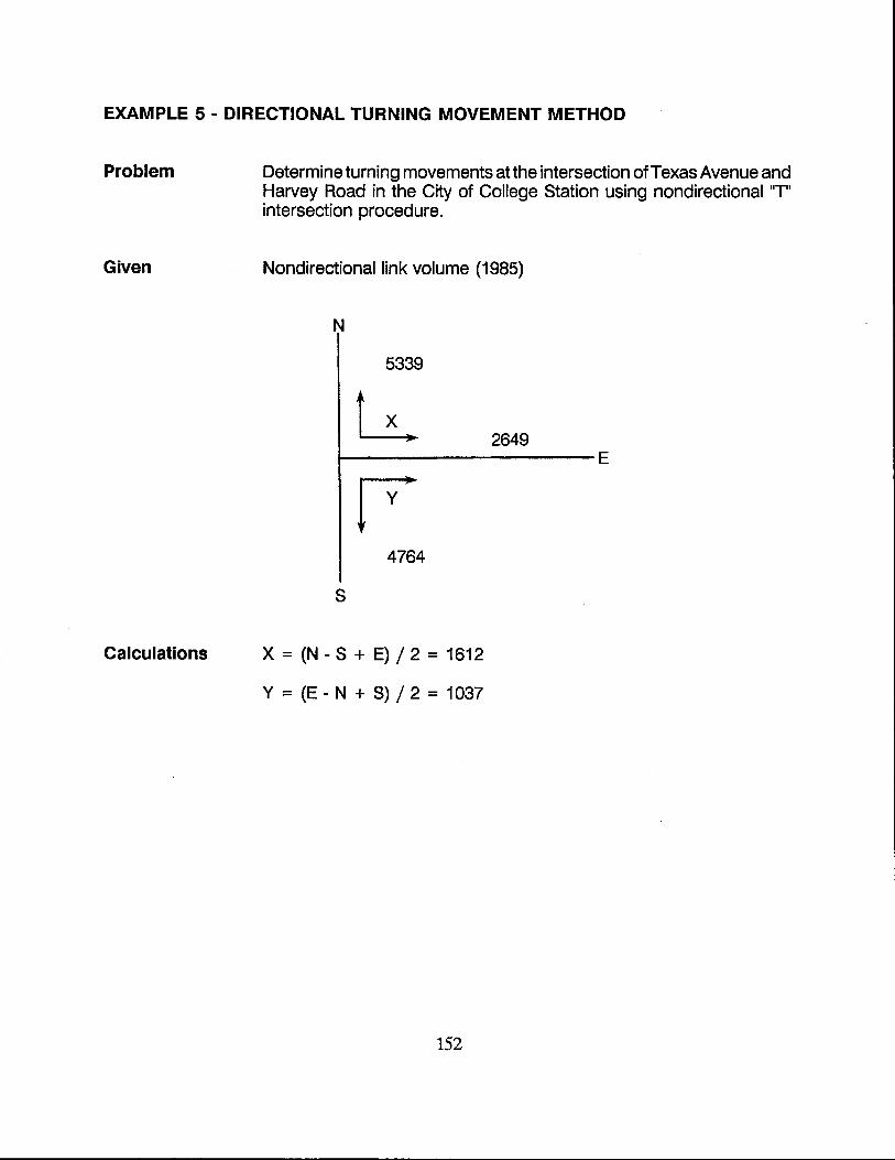
EXAMPLE 5 - DIRECTIONAL TURNING MOVEMENT METHOD
Problem
Given
Calculations
Determine turning movements at the intersection of Texas Avenue and Harvey Road in the City of College Station using nondirectional "T" intersection procedure.
Nondirectional link volume (1985)
N
5339
~ 2649 I----.....--------E
[7 4764
S
x = (N - S + E) / 2 = 1612
Y = (E - N + S) / 2 = 1037
152
APPENDIX F
Development of Theoretical Turning Movements.
153

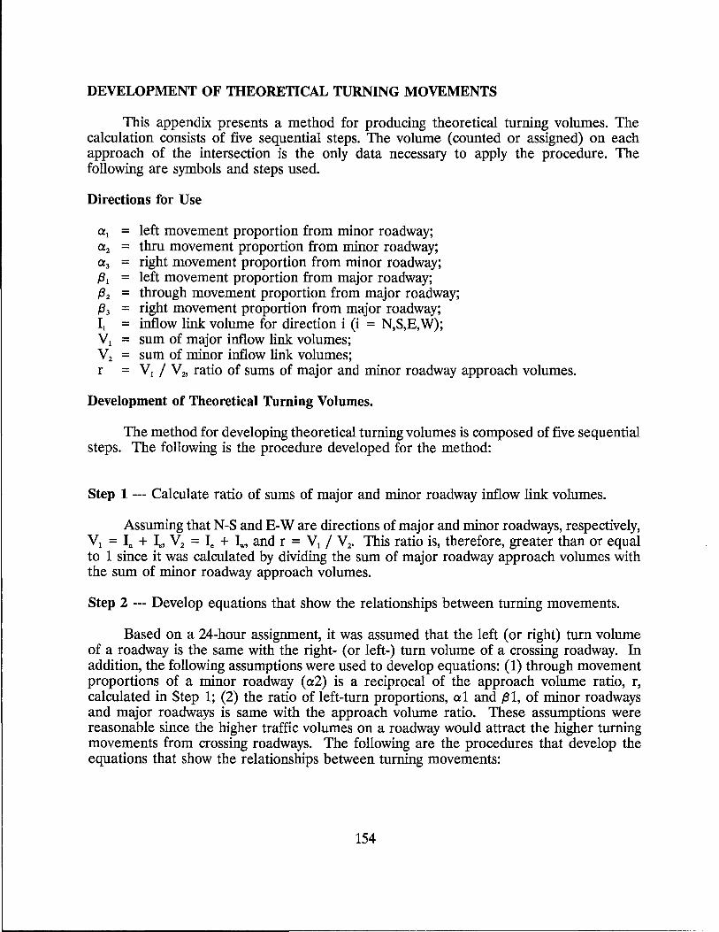
DEVELOPMENT OF THEORETICAL TURNING MOVEMENTS
This appendix presents a method for producing theoretical turning volumes. The calculation consists of five sequential steps. The volume (counted or assigned) on each approach of the intersection is the only data necessary to apply the procedure. The following are symbols and steps used.
Directions for Use
a l
a2 a3 f3I f32 f33 Ii VI V 2
r
= = = = = = = = = =
left movement proportion from minor roadway; thru movement proportion from minor roadway; right movement proportion from minor roadway; left movement proportion from major roadway; through movement proportion from major roadway; right movement proportion from major roadway; inflow link volume for direction i (i = N,S,E,W); sum of major inflow link volumes; sum of minor inflow link volumes; VI / V 2, ratio of sums of major and minor roadway approach volumes.
Development of Theoretical Turning Volumes.
The method for developing theoretical turning volumes is composed of five sequential steps. The following is the procedure developed for the method:
Step 1 --- Calculate ratio of sums of major and minor roadway inflow link volumes.
Assuming that N-S and E-W are directions of major and minor roadways, respectively, VI = In + Is, V 2 = Ie + 4, and r = VI / V 2• This ratio is, therefore, greater than or equal to 1 since it was calculated by dividing the sum of major roadway approach volumes with the sum of minor roadway approach volumes.
Step 2 --- Develop equations that show the relationships between turning movements.
Based on a 24-hour assignment, it was assumed that the left (or right) turn volume of a roadway is the same with the right- (or left-) turn volume of a crossing roadway. In addition, the following assumptions were used to develop equations: (1) through movement proportions of a minor roadway (a2) is a reciprocal of the approach volume ratio, r, calculated in Step 1; (2) the ratio of left-turn proportions, a1 and f31, of minor roadways and major roadways is same with the approach volume ratio. These assumptions were reasonable since the higher traffic volumes on a roadway would attract the higher turning movements from crossing roadways. The following are the procedures that develop the equations that show the relationships between turning movements:
154
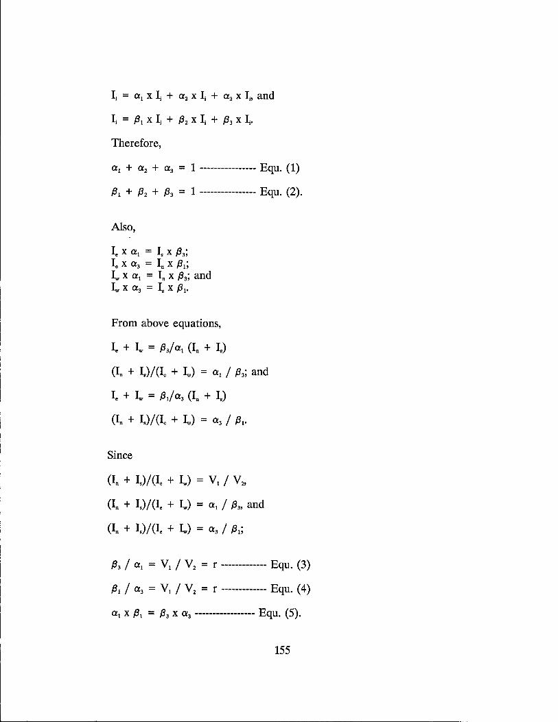
Therefore,
0:1 + 0:2 + 0:3 = 1 ---------------- Equ. (1)
/31 + /32 + /33 = 1 ---------------- Equ. (2).
Also,
Ie X 0:1 = Is X /33;
Ie X 0:3 = In X /31;
4 X 0:1 = In X /33; and 4 X 0:3 = Is X /31"
From above equations,
Ie + Iw = /33/0:1 (In + Is)
(In + Is) / (Ie + 4) = 0:1 / /33; and
Ie + 4 = /31/0:3 (In + Is)
(In + Is)/(Ie + Iw) = 0:3 / /31.
Since
(In + I.)/(Ie + Iw) = VI / V2,
(In + Is)/(Ie + Iw) = 0:1 / /33' and
(In + I.)/(Ie + 4) = 0:3 / /31;
/33 / 0:1 = VI / V2 = r ------------- Equ. (3)
/31 / 0:3 = VI / V2 = r ------------- Equ. (4)
0:1 X /31 = /33 X 0:3 ----------------- Equ. (5).
155
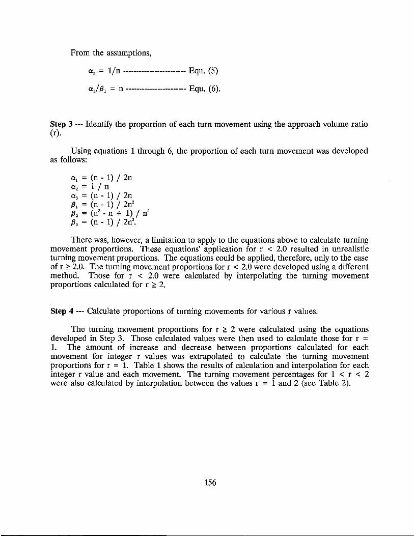
From the assumptions,
aZ = lin ------------------------ Equ. (5)
a1//31 = n ----------------------- Equ. (6).
Step 3 --- Identify the proportion of each turn movement using the approach volume ratio (r).
Using equations 1 through 6, the proportion of each turn movement was developed as follows:
a1 = (n - 1) I 2n az = 1 In a3 = (n - 1) I 2n /31 = (n - 1) I 2nz
/3z = (nZ - n + 1) I nZ
/33 = (n - 1) I 2nz.
There was, however, a limitation to apply to the equations above to calculate turning movement proportions. These equations' application for r < 2.0 resulted in unrealistic turning movement proportions. The equations could be applied, therefore, only to the case of r ~ 2.0. The turning movement proportions for r < 2.0 were developed using a different method. Those for r < 2.0 were calculated by interpolating the turning movement proportions calculated for r ~ 2.
Step 4 --- Calculate proportions of turning movements for various r values.
The turning movement proportions for r ~ 2 were calculated using the equations developed in Step 3. Those calculated values were then used to calculate those for r = 1. The amount of increase and decrease between proportions calculated for each movement for integer r values was extrapolated to calculate the turning movement proportions for r = 1. Table 1 shows the results of calculation and interpolation for each integer r value and each movement. The turning movement percentages for 1 < r < 2 were also calculated by interpolation between the values r = 1 and 2 (see Table 2).
156
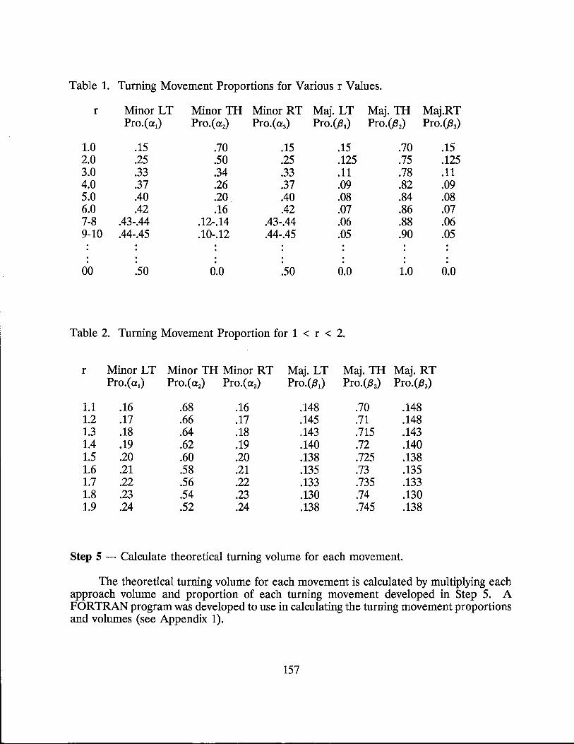
Table 1. Turning Movement Proportions for Various r Values.
r Minor LT Minor TH Minor RT Maj. LT Maj. TH Maj.RT Pro.(a1) Pro. (a2) Pro. (a3) Pro. (.B 1) Pro. (.B2) Pro.(.B3)
1.0 .15 .70 .15 .15 .70 .15 2.0 .25 .50 .25 .125 .75 .125 3.0 .33 .34 .33 .11 .78 .11 4.0 .37 .26 .37 .09 .82 .09 5.0 .40 .20 .40 .08 .84 .08 6.0 .42 .16 .42 .07 .86 .07 7-8 .43-.44 .12-.14 .43-.44 .06 .88 .06 9-10 .44-.45 .10-.12 .44-.45 .05 .90 .05
00 .50 0.0 .50 0.0 1.0 0.0
Table 2. Turning Movement Proportion for 1 < r < 2.
r Minor LT Minor TH Minor RT Maj. LT Maj. TH Maj. RT Pro.(a1) Pro.(a2) Pro.(a3) Pro.(.B1) Pro. (.B2) Pro.(.B3)
1.1 .16 .68 .16 .148 .70 .148 1.2 .17 .66 .17 .145 .71 .148 1.3 .18 .64 .18 .143 .715 .143 1.4 .19 .62 .19 .140 .72 .140 1.5 .20 .60 .20 .138 .725 .138 1.6 .21 .58 .21 .135 .73 .135 1.7 .22 .56 .22 .133 .735 .133 1.8 .23 .54 .23 .130 .74 .130 1.9 .24 .52 .24 .138 .745 .138
Step 5 --- Calculate theoretical turning volume for each movement.
The theoretical turning volume for each movement is calculated by multiplying each approach volume and proportion of each turning movement developed in Step 5. A FORTRAN program was developed to use in calculating the turning movement proportions and volumes (see Appendix 1).
157
APPENDIX G
Counted Approach Volumes and Turning Movements,
Turning Movements As A Percentage of Approach Volume, and
Theoretical Percent Turning Movements.
158

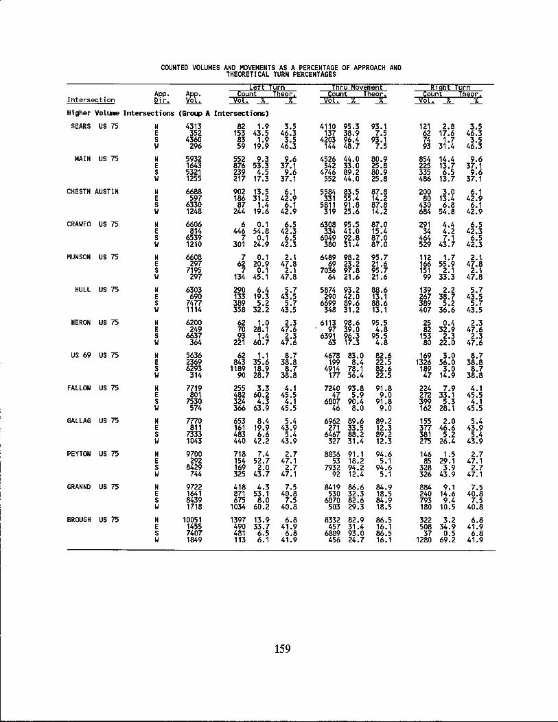
COUNTED VOLUMES AND MOVEMENTS AS A PERCENTAGE OF APPROACH AND THEORETICAL TURN PERCENTAGES
[eH Turn Tfiru Rovement ~19fit Turn App. Ap~. Count Tfieor. Count Tfieor. Count Tfieor.
Intersection Di r. Vo . Vol. % ..!... Vol. % % Vol. % ..!... Higher Volume Intersections (Group A Intersections)
SEARS US 75 N 4313 82 1.9 3.5 4110 95.3 93.1 121 2.8 3.5 E 352 153 43.5 46.3 137 38.9 7.5 62 17.6 46.3 S 4360 83 1.9 3.5 4203 96.4 93.1 74 1.7 3.5 W 296 59 19.9 46.3 144 48.7 7.5 93 31.4 46.3
MAIN US 75 N 5932 552 9.3 9.6 4526 44.0 80.9 854 14.4 9.6 E 1643 876 53.3 37.1 542 33.0 25.8 225 13.7 37.1 S 5321 239 4.5 9.6 4746 89.2 80.9 335 6.5 9.6 W 1255 217 17.3 37.1 552 44.0 25.8 486 13.7 37.1
CHESTN AUSTIN N 6688 902 13.5 6.1 5584 83.5 87.8 200 3.0 6.1 E 597 186 31.2 42.9 331 55.4 14.2 80 13.4 42.9 S 6330 87 1.4 6.1 5811 91.8 87.8 430 6.8 6.1 W 1248 244 19.6 42.9 319 25.6 14.2 684 54.8 42.9
CRAWFO US 75 N 6606 6 0.1 6.5 6308 95.5 87.0 291 4.4 6.5 E 814 446 54.8 42.3 334 41.0 15.4 34 4.2 42.3 S 6539 7 0.1 6.5 6049 92.8 87.0 464 7.1 6.5 W 1210 301 24.9 42.3 380 31.4 87.0 529 43.7 42.3
MUNSON US 75 N 6608 7 0.1 2.1 6489 98.2 95.7 112 1.7 2.1 E 297 62 20.9 47.8 69 23.2 21.6 166 55.9 47.8 S 7195 7 0.1 2.1 7036 97.8 95.7 151 2.1 2.1 W 297 134 45.1 47.8 64 21.6 21.6 99 33.3 47.8
HULL US 75 N 6303 290 6.4 5.7 5874 93.2 88.6 139 2.2 5.7 E 690 133 19.3 43.5 290 42.0 13.1 267 38.7 43.5 S 7477 389 5.2 5.7 6699 89.6 88.6 389 5.2 5.7 W 1114 358 32.2 43.5 348 31.2 13.1 407 36.6 43.5
HERON US 75 N 6200 62 1.0 2.3 6113 98.6 95.5 25 0.4 2.3 E 249 70 28.1 47.6 97 39.0 4.8 82 32.9 47.6 S 6637 93 1.4 2.3 6391 96.3 95.5 153 2.3 2.3 W 364 221 60.7 47.6 63 17.3 4.8 80 22.0 47.6
US 69 US 75 N 5636 62 1.1 8.7 4678 83.0 82.6 169 3.0 8.7 E 2369 843 35.6 38.8 199 8.4 22.5 1326 56.0 38.8 S 6293 1189 18.9 8.7 4914 78.1 82.6 189 3.0 8.7 W 314 90 28.7 38.8 177 56.4 22.5 47 14.9 38.8
FALLON US 75 N 7719 255 3.3 4.1 7240 93.8 91.8 224 7.9 4.1 E 801 482 60.2 45.5 47 5.9 9.0 272 33.1 45.5 S 7530 324 4.3 4.1 6807 90.4 91.8 399 5.3 4.1 W 574 366 63.9 45.5 46 8.0 9.0 162 28.1 45.5
GAL LAG US 75 N 7770 653 8.4 5.4 6962 89.6 89.2 155 2.0 5.4 E 811 161 19.9 43.9 271 33.5 12.3 377 46.6 43.9 S 7333 483 6.6 5.4 6467 88.2 89.2 381 5.2 5.4 W 1043 440 42.2 43.9 327 31.4 12.3 275 26.4 43.9
PEYTON US 75 N 9700 718 7.4 2.7 8836 91.1 94.6 146 1.5 2.7 E 292 154 52.7 47.1 53 18.2 5.1 85 29.1 47.1 S 8429 169 2.0 2.7 7932 94.2 94.6 328 3.9 2.7 W 744 325 43.7 47.1 92 12.4 5.1 326 43.9 47.1
GRANND US 75 N 9722 418 4.3 7.5 8419 86.6 84.9 884 9.1 7.5 E 1641 871 53.1 40.8 530 32.3 18.5 240 14.6 40.8 S 8439 675 8.0 7.5 6870 82.6 84.9 793 9.4 7.5 W 1718 1034 60.2 40.8 503 29.3 18.5 180 10.5 40.8
BROUGH US 75 N 10051 1397 13.9 6.8 8332 82.9 86.5 322 3.2 6.8 E 1455 490 33.7 41.9 457 31.4 16.1 508 34.9 41.9 S 7407 481 6.5 6.8 6889 93.0 86.5 37 0.5 6.8 W 1849 113 6.1 41.9 456 24.7 16.1 1280 69.2 41.9
159
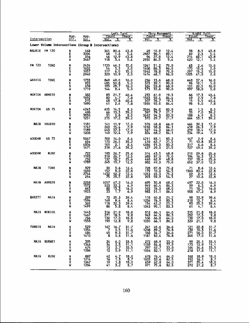
[eft Turn Tliru Rovement ~191it Turn App. Apr· Count Tlieor. Count Tlieor. Count Tlieor.
Intersection Dir. Vo • Vol. l l Vol. % l Vol. % l Lower Volume Intersections (Group B Intersections)
MAURIE FM 120 N 448 361 80.6 43.8 49 10.9 12.4 38 8.5 43.8 E 3004 48 1.6 5.4 2887 96.1 89.1 69 2.3 5.4 S 356 46 12.9 43.8 96 27.0 12.4 214 60.1 43.8 W 3467 118 3.4 5.4 2930 84.5 5.4 420 12.1 5.4
FM 120 TONE N 2424 1120 46.2 15.0 1241 51.2 70.0 63 2.6 15.0 E 1632 54 3.3 2.0 1408 86.3 96.0 170 10.4 2.0 S 1957 117 6.0 15.0 1542 78.8 70.0 297 15.2 15.0 W 2940 320 10.9 2.0 1414 48.1 96.0 1205 41.0 2.0
WASHIG TONE N 1733 849 49.0 16.0 236 13.6 68.0 648 37.4 16.0 E 955 485 50.8 5.0 373 39.1 90.0 96 10.1 5.0 S 638 183 28.7 16.0 324 50.8 68.0 131 20.5 16.0 W 1719 144 8.4 5.0 573 33.6 90.0 997 58.0 5.0
MORTON ARMSTR N 382 83 21.7 40.4 233 61.0 19.3 66 17.3 40.4 E 1692 80 4.7 7.8 1563 92.4 84.4 49 2.9 7.8 S 270 48 17.8 40.4 207 76.7 19.3 15 5.5 40.4 W 1690 41 2.4 7.8 1555 92.0 84.4 95 5.0 7.8
MORTON US 75 N 4243 615 14.5 8.5 3564 84.0 83.0 64 1.5 8.5 E 498 66 13.3 39.2 397 79.7 21.7 35 7.0 39.2 S 3830 31 0.8 8.5 3612 94.3 83.0 188 4.9 8.5 W 1251 215 17.2 39.2 372 29.7 21.7 664 53.1 39.2
MAIN HOUSTO N 1181 141 11.9 17.0 576 48.8 66.0 464 39.3 17.0 E 1747 269 15.4 7.9 1018 58.8 84.1 459 26.3 7.9 S 1189 443 37.3 17.0 527 44.3 66.0 219 18.4 17.0 W 1208 149 12.4 7.9 824 68.2 84.1 234 19.4 7.9
WOOOAR US 75 N 5067 709 14.0 8.4 4211 83.1 83.2 147 2.9 8.4 E 654 173 26.5 39.2 410 62.7 21.5 71 10.8 39.2 S 4804 101 2.1 8.4 4386 91.3 83.2 317 6.6 8.4 W 1471 318 21.6 39.2 427 29.0 21.5 727 49.4 39.2
WOODAR RUSK N 722 193 26.7 25.6 314 43.5 48.8 215 29.8 25.6 E 1193 319 26.7 12.5 680 57.0 75.0 194 16.3 12.5 S 732 137 18.7 25.6 460 62.9 48.8 137 18.4 25.6 W 1789 245 13.7 12.5 882 49.3 75.0 652 37.0 12.5
MAIN TONE N 829 30 3.6 12.4 728 87.8 75.2 71 8.6 12.4 E 1692 152 9.0 22.8 179 10.6 54.5 1360 80.4 22.8 S 2744 1432 52.2 12.4 1243 45.3 75.2 69 2.5 12.4 W 254 75 29.5 22.8 203 59.9 54.5 27 10.6 22.8
MAIN ARMSTR N 2258 1057 47.2 16.0 695 30.8 68.0 497 22.0 16.0 E 1572 523 33.3 6.9 949 60.4 86.3 99 6.3 6.9 S 663 88 13.3 16.0 503 76.0 68.0 71 10.7 16.0 W 1923 33 1.7 6.9 983 51.1 86.0 908 47.2 6.9
BARETT MAIN N 289 73 25.3 39.4 118 40.8 21.2 98 33.9 39.4 E 1594 149 9.4 8.4 1256 76.9 83.3 218 13.7 8.4 S 365 118 32.3 39.4 154 42.2 21.2 93 25.5 39.4 W 1491 86 5.8 8.4 1343 90.1 83.3 61 4.1 8.4
MAIN MIRICK N 1443 316 21.9 18.0 812 66.1 64.0 315 21.8 18.0 E 1467 271 18.5 9.8 943 64.3 80.3 252 17.3 9.8 S 766 130 17.0 18.0 506 66.0 64.0 130 17.0 18.0 W 1558 199 12.8 9.8 1030 66.1 80.3 329 21.1 9.8
FANNIN MAIN N 529 167 16.7 31.7 241 45.6 36.6 121 22.8 31.7 E 1354 7 0.5 11.6 1208 89.2 76.8 139 10.3 11.6 S 484 45 9.3 31.7 168 34.7 36.6 271 56.0 31.7 W 1410 8 0.6 11.6 1161 82.4 76.8 240 17.0 11.6
MAIN BURNET N 395 24 6.0 33.5 272 68.9 33.0 99 25.1 33.5 E 1346 34 2.5 11.1 1139 84.6 77.9 173 12.9 11.1 S 474 13 2.7 33.5 297 62.7 33.0 164 34.6 33.5 W 1286 12 0.9 11.1 1056 82.1 77.9 218 17.0 11.1
MAIN RUSK N 887 42 4.7 18.0 678 76.4 64.0 168 18.9 18.0 E 1214 16 1.3 8.7 1003 82.6 82.5 192 16.1 8.7 S 1047 19 1.8 18.0 659 62.8 64.0 371 35.4 18.0 W 1284 41 3.2 8.7 971 75.6 82.5 272 21.2 8.7
160
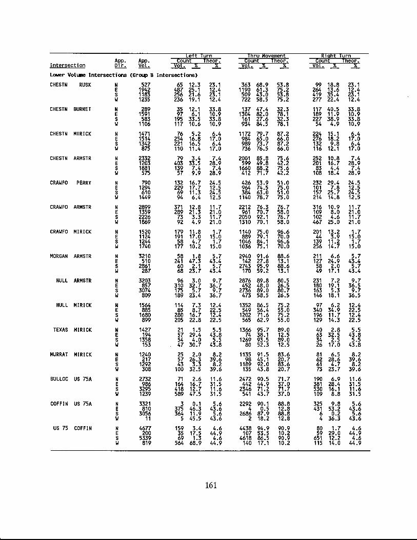
[eft Turn Tliru Movement ~181it Turn App. A~. Count Tlieor. Count Tlieor. Count Tlieor.
Intersection Dir. Vo • Vol. l l Vol. % % Vol. l %
Lower Volume Intersections (Group B Intersections)
CHESTN RUSK N 527 65 12.3 23.1 363 68.9 53.8 99 18.8 23.1 E 1942 487 25.1 12.4 1190 61.3 75.2 264 13.6 12.4 S 1183 256 21.6 23.1 509 43.0 53.8 419 35.4 23.1 W 1235 236 19.1 12.4 722 58.5 75.2 2n 22.4 12.4
CHESTN BURNET N 289 35 12.1 33.8 137 47.4 32.3 117 40.5 33.8 E 1591 97 6.1 10.9 1304 82.0 78.1 189 11.9 10.9 S 583 195 33.5 33.8 161 27.6 32.3 227 38.9 33.8 W 1106 117 10.6 10.9 934 84.5 78.1 54 4.9 10.9
CHESTN MIRICK N 1471 76 5.2 6.4 1172 79.7 87.2 224 15.1 6.4 E 1514 254 16.8 17.0 984 65.0 66.0 276 18.2 17.0 S 1342 221 16.5 6.4 989 73.7 87.2 132 9.8 6.4 W 875 110 11.4 17.0 736 76.5 66.0 116 12.1 17.0
CHESTN ARMSTR N 2332 79 3.4 7.4 2001 85.8 75.6 252 10.8 7.4 E 1203 403 33.5 28.9 599 49.8 42.2 201 16.7 28.9 S 1881 139 7.4 7.4 1660 88.2 75.6 83 4.4 7.4 W 575 57 9.9 28.9 412 71.7 42.2 108 18.4 28.9
CRAWFO PERRY N 790 132 16.7 24.5 426 53.9 51.0 232 29.4 24.5 E 1294 229 17.7 12.5 964 74.5 75.0 101 7.8 12.5 S 610 69 11.3 24.5 384 63.0 51.0 157 25.7 24.5 W 1449 94 6.4 12.5 1140 78.7 75.0 214 14.8 12.5
CRAWFO ARMSTR N 2899 371 12.8 11.7 2212 76.3 76.7 316 10.9 11.7 E 1359 289 21.3 21.0 961 70.7 58.0 109 8.0 21.0 S 2226 73 3.3 11.7 2050 92.1 76.7 102 4.6 11.7 W 1869 92 4.9 21.0 1310 70.1 58.0 467 25.0 21.0
CRAWFO MIRICK N 1520 179 11.8 1.7 1140 75.0 96.6 201 13.2 1.7 E 1124 191 17.0 15.0 889 79.1 70.0 44 3.9 15.0 S 1244 58 4.7 1.7 1046 84.1 96.6 139 11.2 1.7 W 1740 177 10.2 15.0 1036 75.1 70.0 256 14.7 15.0
MORGAN ARMSTR N 3210 58 1.8 5.7 2940 91.6 88.6 211 6.6 5.7 E 510 241 47.3 43.4 142 27.8 13.1 127 24.9 43.4 S 2861 60 2.1 5.7 2743 95.9 88.6 58 2.0 5.7 W 287 68 23.7 43.4 170 59.2 13.1 49 17.1 43.4
HULL ARMSTR N 3203 96 3.0 9.7 2876 89.8 80.5 231 7.2 9.7 E 857 310 32.7 36.7 452 48.0 26.5 180 19.1 36.5 S 3074 175 5.7 9.7 2736 89.0 80.7 163 5.3 9.7 W 809 189 23.4 36.7 473 58.5 26.5 146 18.1 36.5
HULL MIRICK N 1564 114 7.3 12.4 1352 86.5 75.2 97 6.2 12.4 E 885 85 8.7 22.5 549 56.4 55.0 340 34.9 22.5 S 1680 280 16.7 12.4 1202 71.6 75.2 196 11.7 12.4 W 899 205 22.8 22.5 565 62.9 55.0 129 14.3 22.5
TEXAS MIRICK N 1427 21 1.5 5.5 1366 95.7 89.0 40 2.8 5.5 E 194 57 29.4 43.8 74 38.1 12.5 63 32.5 43.8 S 1358 54 4.0 5.5 1269 93.5 89.0 34 2.5 5.5 W 153 47 30.7 43.8 80 52.3 12.5 26 17.0 43.8
MURRAT MIRICK N 1240 25 2.0 8.2 1135 91.5 83.6 81 6.5 8.2 E 217 57 26.3 39.6 98 45.1 20.7 62 28.6 39.6 S 1292 43 3.3 8.2 1189 92.0 83.6 61 4.7 8.2 W 308 100 32.5 39.6 135 43.8 20.7 73 23.7 39.6
BULLOC US 75A N 2732 71 2.6 11.6 2472 90.5 71.7 190 6.9 11.6 E 986 164 16.7 31.5 442 44.9 37.0 381 28.4 31.5 S 3295 418 12.7 11.6 2346 71.2 71.7 530 16.1 11.6 W 1239 589 47.5 31.5 541 43.7 37.0 109 8.8 31.5
COFFIN US 75A N 3321 3 0.1 5.6 2292 90.1 88.8 325 9.8 5.6 E 810 375 46.3 43.6 4 0.5 12.8 431 53.2 43.6 S 3056 364 11.9 5.6 2686 87.9 88.8 6 0.2 5.6 W 11 5 45.5 43.6 2 18.2 12.8 4 36.3 43.6
US 75 COFFIN N 4677 159 3.4 4.6 4438 94.9 90.9 80 1.7 4.6 E 200 35 17.5 44.9 107 53.5 10.2 59 29.0 44.9 S 5339 69 1.3 4.6 4618 86.5 90.9 651 12.2 4.6 W 819 564 68.9 44.9 140 17.1 10.2 115 14.0 44.9
161
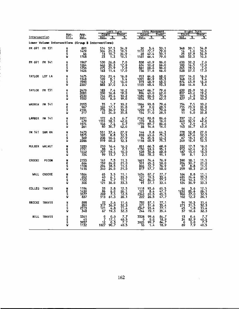
[eft Turn T~ru Rovement Ih~~t Turn App. Apr' Count T~eor. Count Tlieor. Coun· Tlieor.
Intersection Dir. Vo . Vol. l % Vol. % % Vol. % l Lower Volume Intersections (Group B Intersections)
FM 691 FM 131 N 891 514 57.5 34.9 30 3.4 30.1 348 39.1 34.9 E 1429 304 21.3 10.5 1110 77.7 79.0 14 1.0 10.5 S 66 13 19.7 34.9 28 42.4 30.1 25 37.9 34.9 W 1748 23 1.3 10.5 1161 66.4 79.0 565 32.3 10.5
FM 691 FM 141 N 1967 530 26.8 7.0 808 40.9 86.0 638 32.3 7.0 E 1264 446 35.3 17.0 634 50.2 66.0 183 14.5 17.0 S 1256 275 21.9 7.0 861 68.6 86.0 245 19.5 7.0 W 1426 163 11.4 17.0 736 51.6 66.0 528 37.0 17.0
TAYLOR LOY LA N 1475 316 21.4 16.0 953 64.6 68.0 207 14.0 16.0 E 1348 109 8.1 3.4 1091 80.9 93.3 148 11.0 3.4 S 1990 143 7.2 16.0 973 48.9 68.0 874 43.9 16.0 W 2387 883 37.0 3.4 1155 48.4 93.3 348 14.6 3.4
TAYLOR FM 131 N 2470 183 7.4 10.2 1647 66.7 79.6 639 25.9 10.2 E 2081 350 16.8 19.0 894 43.0 62.0 837 40.2 19.2 S 2530 744 29.4 10.2 1685 66.6 79.6 101 4.0 10.2 W 1502 120 8.0 19.0 1054 70.2 62.0 327 21.8 10.2
WASHIN FM 141 N 2053 35 1.7 10.2 1864 90.8 79.6 154 7.5 10.2 E 967 165 17.1 35.8 87 9.0 28.5 715 73.9 35.8 S 2104 776 36.9 10.2 1290 61.3 79.6 38 1.8 10.2 W 217 52 24.0 35.8 154 71.0 28.5 11 5.0 35.8
LAMBER FM 141 N 2651 172 6.5 6.7 2142 80.8 86.6 337 12.7 6.7 E 479 1155 58.5 42.0 170 8.6 16.0 649 32.9 42.0 S 1974 146 7.4 6.7 1770 89.7 86.6 57 2.9 6.7 W 261 80 30.7 42.0 38 14.6 16.0 143 54.7 42.0
FM 141 SAM RA N 1473 551 37.4 27.9 144 9.8 44.3 778 52.8 27.9 E 1875 165 8.8 12.3 818 43.6 75.3 893 47.6 12.3 S 369 208 56.4 27.9 94 25.5 44.3 67 18.1 27.9 W 2286 919 40.2 12.3 1118 48.9 75.3 249 10.9 12.3
MULBER WALNUT N 1283 210 16.4 16.0 851 66.3 68.0 222 17.3 16.0 E 2151 88 4.1 2.5 1150 53.5 95.1 912 42.4 2.5 S 1442 727 50.4 16.0 528 36.6 68.0 187 13.0 16.0 W 724 99 13.7 2.5 566 78.2 95.1 59 8.1 2.5
CROCKE PECON N 2153 161 7.5 11.5 1601 74.4 76.9 390 18.1 11.5 E 664 159 24.0 21.0 301 45.3 58.0 204 30.7 21.0 S 1108 204 18.5 11.5 806 72.7 76.9 97 8.8 11.5 W 1416 340 24.0 21.0 817 57.7 58.0 259 18.3 21.0
WALL CROCKE N 1864 65 3.5 11.1 1634 87.7 77.7 164 8.8 11.1 E 652 40 6.1 33.3 127 19.5 33.4 485 74.4 33.3 S 1122 64 5.7 11.1 942 84.0 77.7 116 10.3 11. 1 W 306 121 36.0 33.3 91 27.1 33.4 124 36.9 33.3
COL LEG TRAVIS N 1194 33 2.8 12.5 1118 93.6 65.5 44 3.6 12.5 E 1439 86 6.0 26.1 121 8.4 47.7 1232 85.6 26.1 S 3577 269 7.5 12.5 2342 65.5 65.5 966 27.0 12.5 W 837 513 61.3 26.1 222 26.5 47.7 102 12.2 26.1
RROCKE TRAVIS N 898 22 2.4 11.4 782 87.1 77.1 94 10.5 11.4 E 859 317 36.9 32.3 271 31.6 35.4 271 31.5 32.3 S 2513 121 4.8 11.4 2347 93.4 77.1 45 1.8 11.4 W 348 67 19.3 32.3 244 70.1 35.4 37 10.6 32.3
HILL TRAVIS N 3341 0 0.0 7.7 3328 99.6 84.7 13 0.4 7.7 E 41 7 17.1 40.5 0 0.0 18.9 34 82.9 40.5 S 3937 12 0.3 7.7 3925 99.7 84.7 0 0.0 7.7 W 1132 1027 90.7 40.5 16 1.4 18.9 89 7.9 40.5
162