traffic flows mesoscopic simulation...

D R . S C . I N G . M I H A I L S S AV R A S O V S

T R A N S P O R T A N D T E L E C O M M U N I C AT I O N I N S T I T U T E

R I G A , L AT V I A

TRAFFIC FLOW SIMULATION USING

MESOSCOPIC APPROACH

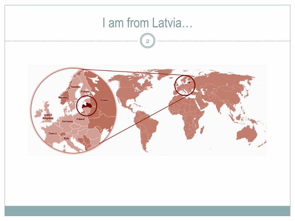
I am from Latvia…2

Time line3

Higher Military

School for Aviation

Engineers (Riga)

1946

Riga Institute for

Civil Aviation

Engineers (Riga)

1960

1992

Riga Aviation

University

TSI

University of

applied

sciences

1999

Aircraft Technician

School (Kiev)

1919

Key data4

Number of students: > 2900

Faculties:

Computer Science and Telecommunication

Management and Economics

Transport and Logistics

Levels:

Bachelor/Professional qualification

Master

PhD

Staff: >160 teaching staff

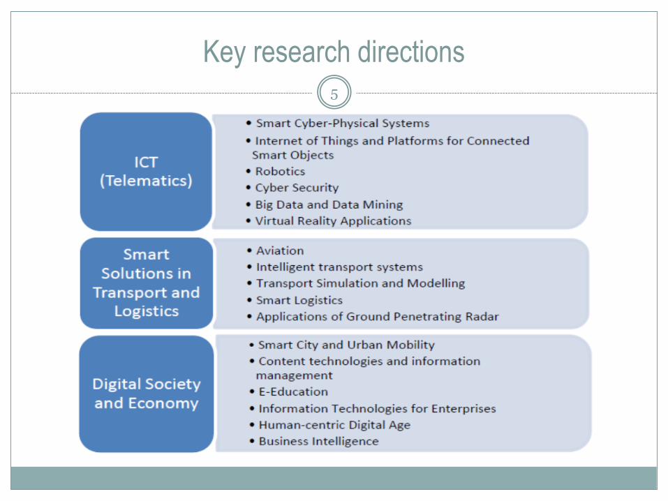
Key research directions5

Contents7

Introduction

Fundamentals of mesoscopic discrete rate

approach

Formulation of discrete rate traffic reference model

Case-study: simulation of the two connected

crossroads

Case-study: Urban transport corridor mesoscopic

simulation

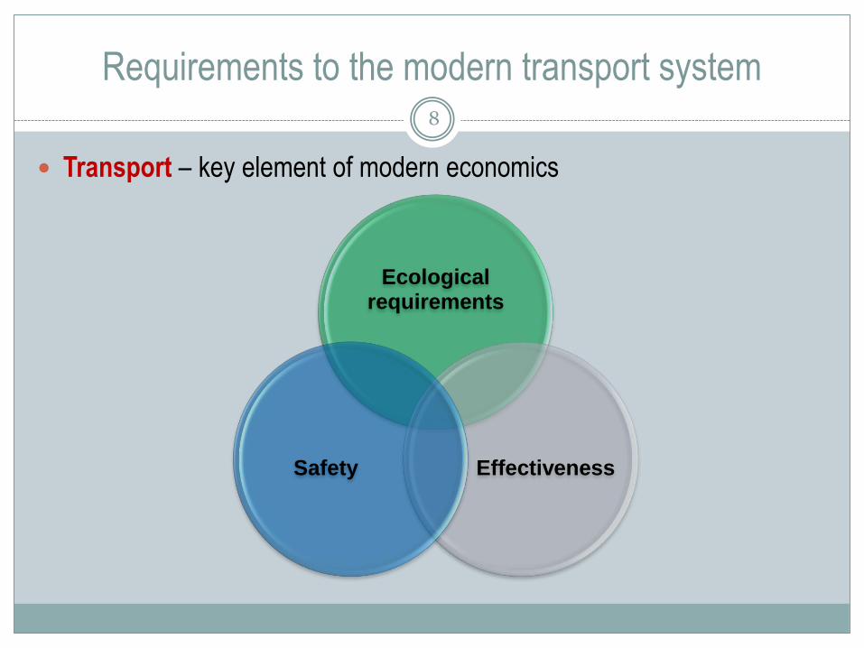
Requirements to the modern transport system8

Transport – key element of modern economics

Ecological requirements

EffectivenessSafety

Sustainable development9

Sustainable development is a development that meets the needs of the present without compromising the ability of future generations to meet their own needs

Transport sustainable development tools: use of ITS (Intelligent Transportation Systems)

use of P&R (Park and Ride)

optimization of existing transport infrastructure

development of intermodality

implementation of new transport infrastructure elements onthe base of doing strict impact analysis

use of sound tax policy

etc

Traffic analysis tools10

A traffic analysis tools is a collective term used to describe a variety of

software-based analytical procedures and methodologies that support

different aspects of traffic and transportation analyses

Traffic analysis tools:

• Sketch –planning tools

• Travel demand models

• Analytical deterministic tools (HCM, ICU…)

• Traffic signal optimization tools

• Macroscopic simulation models

• Mesoscopic simulation models

• Microscopic simulation models

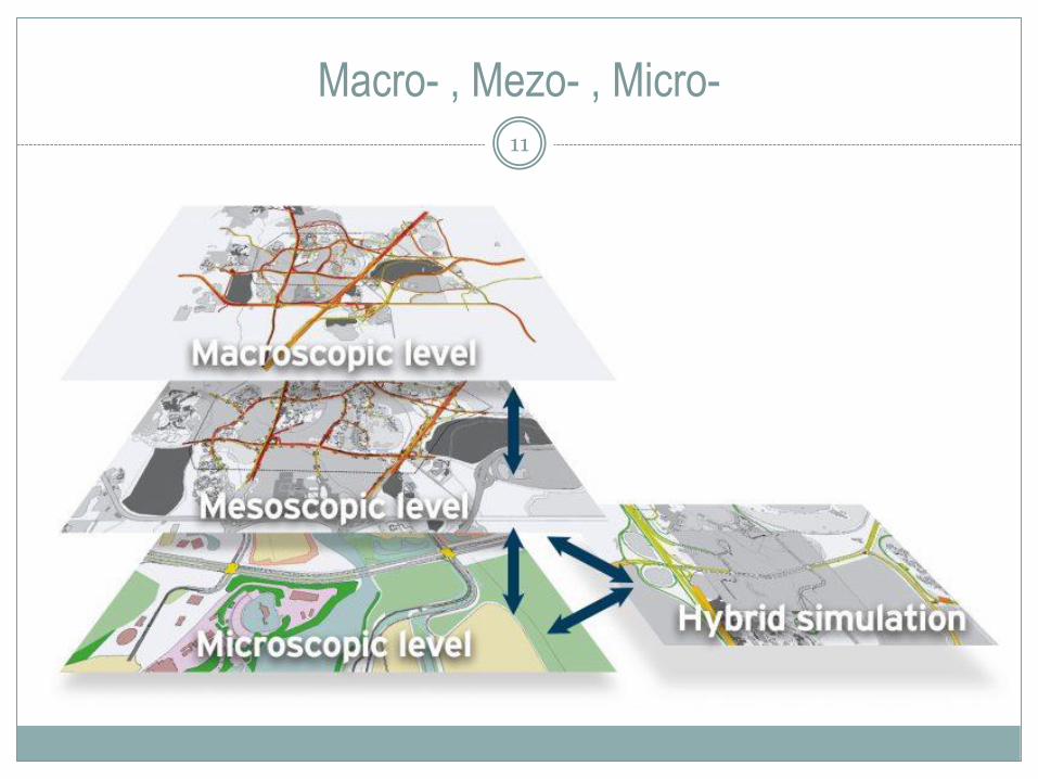
Macro- , Mezo- , Micro-11

Mesoscopic models12

Mesoscopic models combine the properties of both microscopic and macroscopic simulation models. These models simulate individual vehicles, but describe their activities and interactions based on aggregate (macroscopic) relationships 1

Mesoscopic models of traffic flow are based on estimation macroscopic indices on microscopic level 2

Mesoscopic models combine the properties of both microscopic and macroscopic simulation models. These models simulate individual vehicles or group of vehicles, but describe their activities and interactions based on aggregate (macroscopic) relationships

1) http://www.dot.ca.gov

2) Gilkerson G. et al. 2005. Traffic Simulation

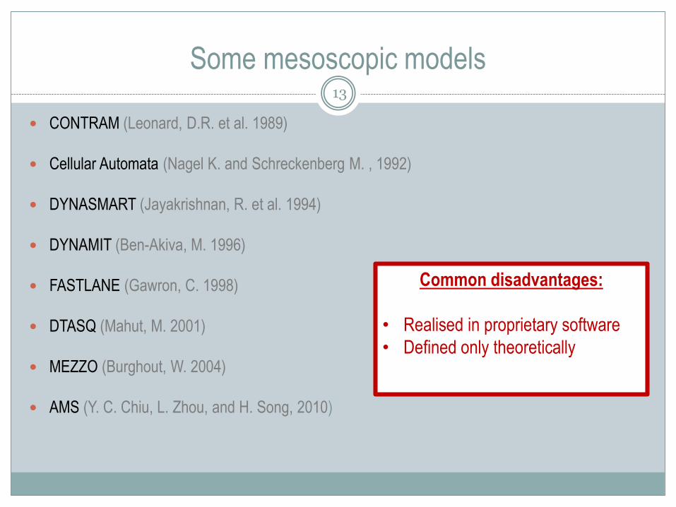
Some mesoscopic models

СONTRAM (Leonard, D.R. et al. 1989)

Cellular Automata (Nagel K. and Schreckenberg M. , 1992)

DYNASMART (Jayakrishnan, R. et al. 1994)

DYNAMIT (Ben-Akiva, M. 1996)

FASTLANE (Gawron, C. 1998)

DTASQ (Mahut, M. 2001)

MEZZO (Burghout, W. 2004)

AMS (Y. C. Chiu, L. Zhou, and H. Song, 2010)

13

Common disadvantages:

• Realised in proprietary software

• Defined only theoretically

14

Fundamentals of

discrete rate approach

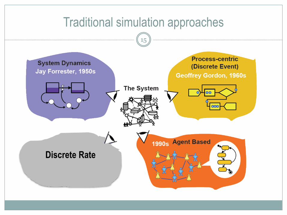
Traditional simulation approaches15

Discrete Rate

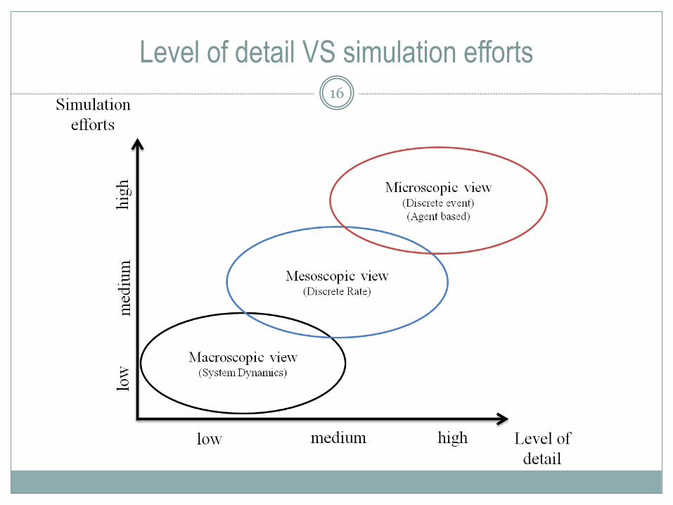
Level of detail VS simulation efforts16

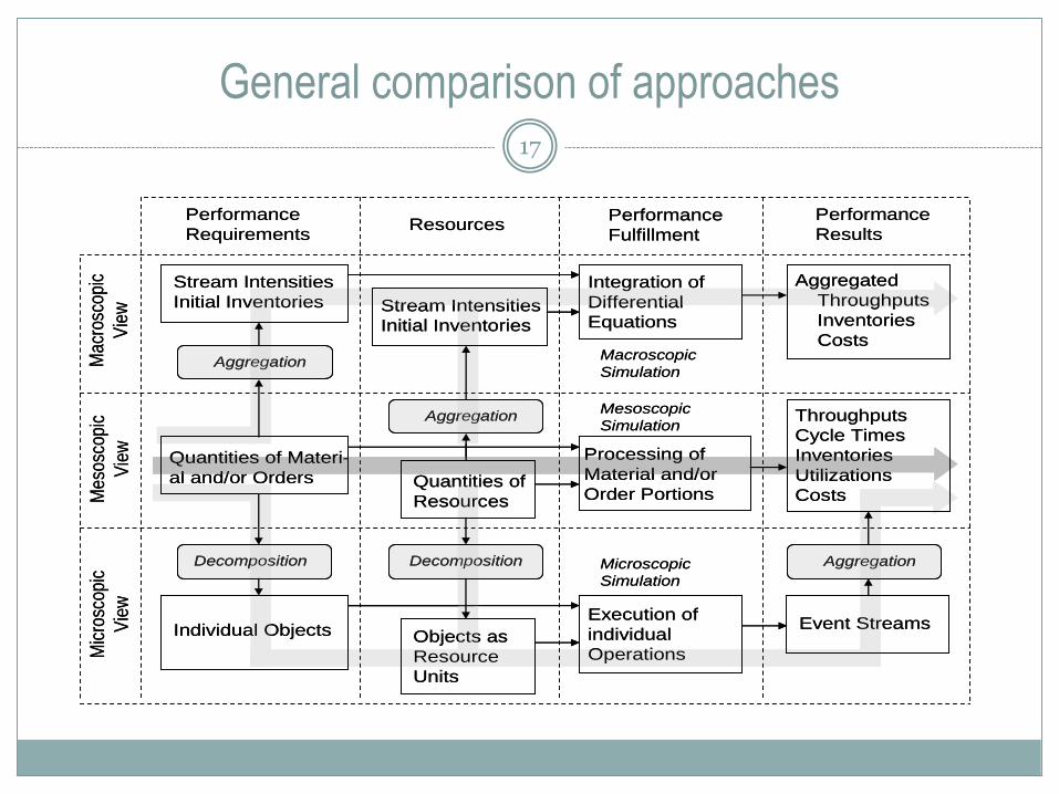
General comparison of approaches17

Performance

RequirementsResources

Performance

Fulfillment

Performance

Results

Quantities of Materi-

al and/or Orders Quantities of

Resources

Processing of

Material and/or

Order Portions

Throughputs

Cycle Times

Inventories

Utilizations

Costs

Individual Objects Objects as

Resource

Units

Execution of

individual

Operations

Event Streams

Decomposition Decomposition

Mes

osco

pic

Vie

w

Mic

rosc

opic

Vie

w

Aggregation

Mesoscopic

Simulation

Microscopic

Simulation

Aggregation

Stream Intensities

Initial Inventories

Integration of

Differential

Equations

Aggregated

Throughputs

Inventories

CostsMacroscopic

Simulation

Aggregation

Stream Intensities

Initial Inventories

Mac

rosc

opic

Vie

w

Performance

RequirementsResources

Performance

Fulfillment

Performance

Results

Quantities of Materi-

al and/or Orders Quantities of

Resources

Processing of

Material and/or

Order Portions

Throughputs

Cycle Times

Inventories

Utilizations

Costs

Individual Objects Objects as

Resource

Units

Execution of

individual

Operations

Event Streams

Decomposition Decomposition

Mes

osco

pic

Vie

w

Mic

rosc

opic

Vie

w

Aggregation

Mesoscopic

Simulation

Microscopic

Simulation

Aggregation

Stream Intensities

Initial Inventories

Integration of

Differential

Equations

Aggregated

Throughputs

Inventories

CostsMacroscopic

Simulation

Aggregation

Stream Intensities

Initial Inventories

Mac

rosc

opic

Vie

w

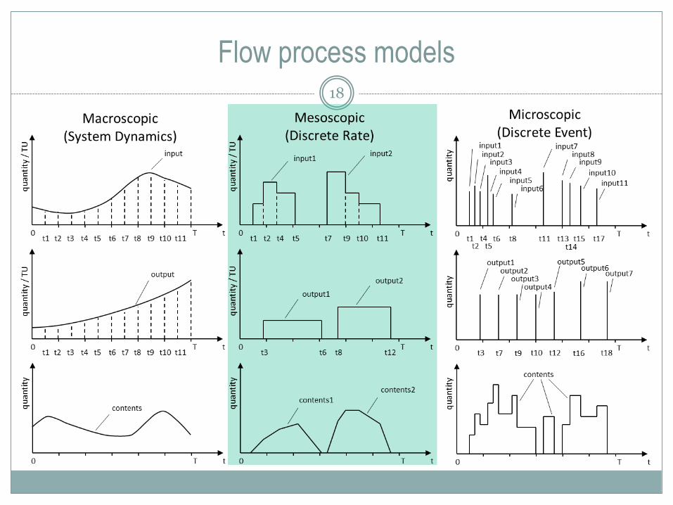
Flow process models18

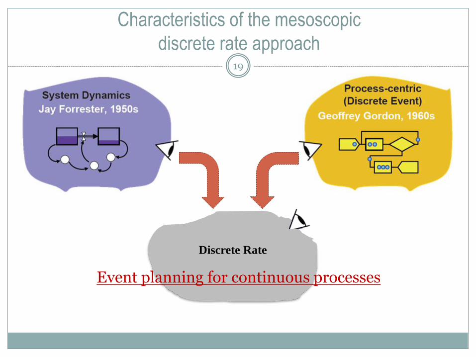
Characteristics of the mesoscopic

discrete rate approach19

Discrete Rate

Event planning for continuous processes

Hybrid characteristics of a mesoscopic discrete rate

approach20

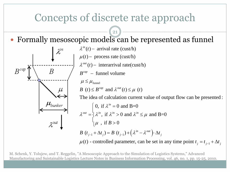
Concepts of discrete rate approach

Formally mesoscopic models can be represented as funnel

funnel

( ) arrival rate (cust/h)

( ) process rate (cust/h)

( ) interarrival rate(cust/h)

funnel volume

( ) and ( ) ( )

The idea of calculation current value of output flow c

in

out

cap

cap out

t

t

t

B

B t B t t

1 1

1

an be presented :

0, if 0 and B=0

, if 0 and and B=0

, if 0

( ) ( )

( ) - controlled parameter, can be set in any time point

in

out in in in

in out

j j j j

j j j

B

B t t B t t

t t t t

21

M. Schenk, Y. Tolujew, and T. Reggelin, "A Mesoscopic Approach to the Simulation of Logistics Systems," Advanced Manufactoring and Suistainable Logistics Lecture Notes in Business Information Processing, vol. 46, no. 1, pp. 15-25, 2010.

M O D E L F O R U N C O N G E S T E D N E T W O R K

M O D E L F O R C O N G E S T E D N E T W O R K

22

Formulation of DRTRM

(discrete rate traffic reference model)

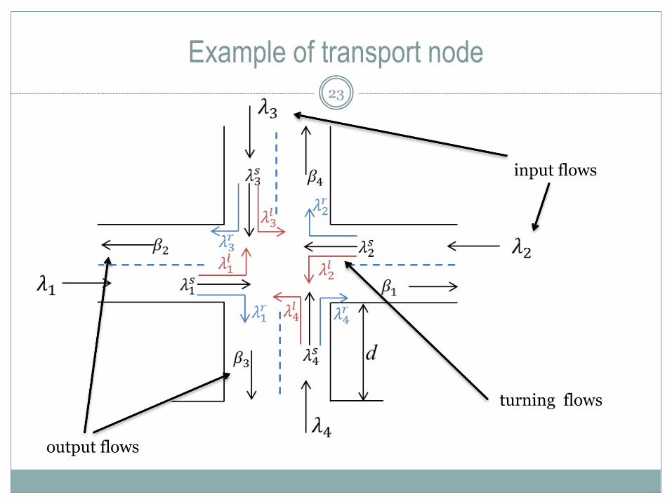
Example of transport node23

input flows

output flows

turning flows

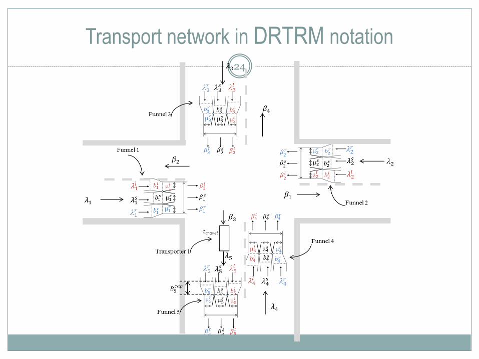
Transport network in DRTRM notation

24

2

2

2

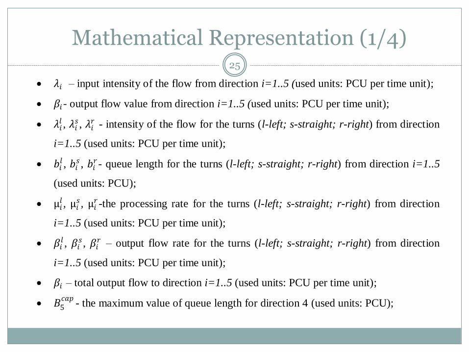
Mathematical Representation (1/4)25

• 𝜆𝑖 – input intensity of the flow from direction i=1..5 (used units: PCU per time unit);

• 𝛽𝑖- output flow value from direction i=1..5 (used units: PCU per time unit);

• 𝜆𝑖𝑙 , 𝜆𝑖

𝑠 , 𝜆𝑖𝑟 - intensity of the flow for the turns (l-left; s-straight; r-right) from direction

i=1..5 (used units: PCU per time unit);

• 𝑏𝑖𝑙 , 𝑏𝑖

𝑠 , 𝑏𝑖𝑟 - queue length for the turns (l-left; s-straight; r-right) from direction i=1..5

(used units: PCU);

• µ𝑖𝑙 , µ𝑖

𝑠 , µ𝑖𝑟 -the processing rate for the turns (l-left; s-straight; r-right) from direction


• 𝛽𝑖𝑙 , 𝛽𝑖

𝑠 , 𝛽𝑖𝑟 – output flow rate for the turns (l-left; s-straight; r-right) from direction


• 𝛽𝑖 – total output flow to direction i=1..5 (used units: PCU per time unit);

• 𝐵5𝑐𝑎𝑝

- the maximum value of queue length for direction 4 (used units: PCU);

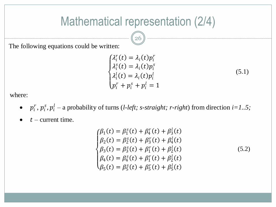
Mathematical representation (2/4)26

The following equations could be written:

𝜆𝑖

𝑟 𝑡 = 𝜆𝑖 𝑡 𝑝𝑖𝑟

𝜆𝑖𝑠 𝑡 = 𝜆𝑖 𝑡 𝑝𝑖

𝑠

𝜆𝑖𝑙 𝑡 = 𝜆𝑖 𝑡 𝑝𝑖

𝑙

𝑝𝑖𝑟 + 𝑝𝑖

𝑠 + 𝑝𝑖𝑙 = 1

(5.1)

where:

• 𝑝𝑖𝑟 , 𝑝𝑖

𝑠 , 𝑝𝑖𝑙 – a probability of turns (l-left; s-straight; r-right) from direction i=1..5;

• 𝑡 – current time.

𝛽1 𝑡 = 𝛽1

𝑠 𝑡 + 𝛽4𝑟 𝑡 + 𝛽3

𝑙 𝑡

𝛽2 𝑡 = 𝛽2𝑠 𝑡 + 𝛽3

𝑟 𝑡 + 𝛽4𝑙 𝑡

𝛽3 𝑡 = 𝛽3𝑠 𝑡 + 𝛽1


𝛽4 𝑡 = 𝛽4𝑠 𝑡 + 𝛽1


𝛽5 𝑡 = 𝛽5𝑠 𝑡 + 𝛽5


(5.2)

Mathematical representation (3/4)27

𝛽𝑖∈(1,2,4,5)𝑠 𝑡 =

0, 𝜆𝑖𝑠 𝑡 = 0 𝑎𝑛𝑑 𝑏𝑖

𝑠 𝑡 = 0

𝜆𝑖𝑠 𝑡 ,𝜆𝑖

𝑠 𝑡 > 0 𝑎𝑛𝑑 𝜆𝑖𝑠 𝑡 ≤ 𝜇𝑖

𝑠 𝑎𝑛𝑑 𝑏𝑖𝑠 𝑡 = 0

𝜇𝑖𝑠 , 𝑏𝑖

𝑠 𝑡 > 0

(5.4)

𝛽𝑖∈(2,3,4,5)𝑟 𝑡 =

0, 𝜆𝑖𝑟 𝑡 = 0 𝑎𝑛𝑑 𝑏𝑖

𝑟 𝑡 = 0

𝜆𝑖𝑟 𝑡 ,𝜆𝑖

𝑟 𝑡 > 0 𝑎𝑛𝑑 𝜆𝑖𝑟 𝑡 ≤ 𝜇𝑖

𝑟 𝑎𝑛𝑑 𝑏𝑖𝑟 𝑡 = 0

𝜇𝑖𝑟 , 𝑏𝑖

𝑟 𝑡 > 0

(5.5)

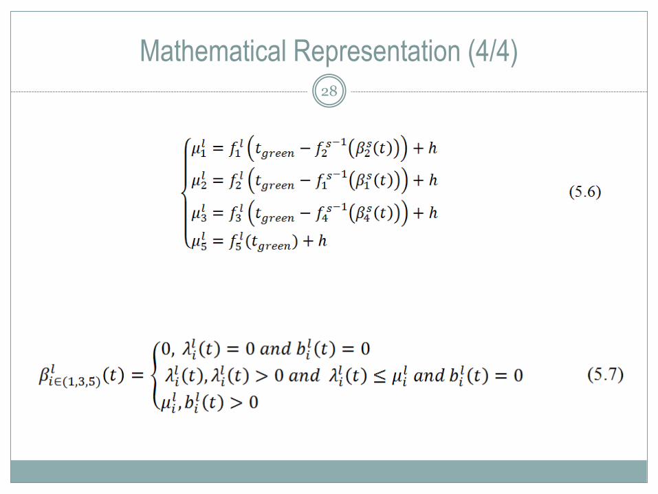
Mathematical Representation (4/4)28

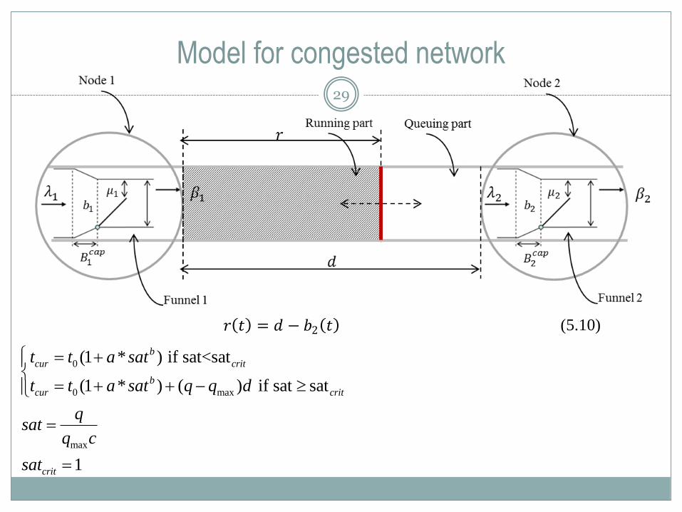
Model for congested network29

𝑟 𝑡 = 𝑑 − 𝑏2 𝑡 (5.10)

0

0 max

max

(1 * ) if sat<sat

(1 * ) ( ) if sat sat

1

b

cur crit

b

cur crit

crit

t t a sat

t t a sat q q d

qsat

q c

sat

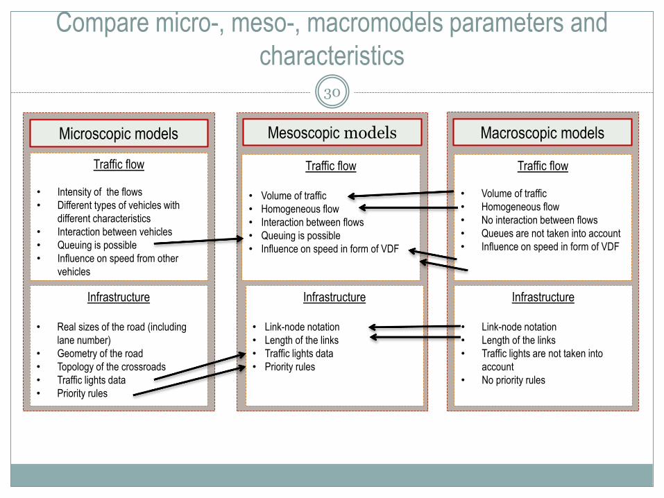
Compare micro-, meso-, macromodels parameters and

characteristics 30

Microscopic models Macroscopic models

Traffic flow

• Intensity of the flows

• Different types of vehicles with

different characteristics

• Interaction between vehicles

• Queuing is possible

• Influence on speed from other

vehicles

Infrastructure

• Real sizes of the road (including

lane number)

• Geometry of the road

• Topology of the crossroads

• Traffic lights data

• Priority rules

Traffic flow

• Volume of traffic

• Homogeneous flow

• No interaction between flows

• Queues are not taken into account

• Influence on speed in form of VDF

Infrastructure

• Link-node notation

• Length of the links

• Traffic lights are not taken into

account

• No priority rules

Traffic flow

• Volume of traffic

• Homogeneous flow

• Interaction between flows

• Queuing is possible

• Influence on speed in form of VDF

Infrastructure

• Link-node notation

• Length of the links

• Traffic lights data

• Priority rules

Mesoscopic models

Case-study: simulation of the two

connected crossroads31

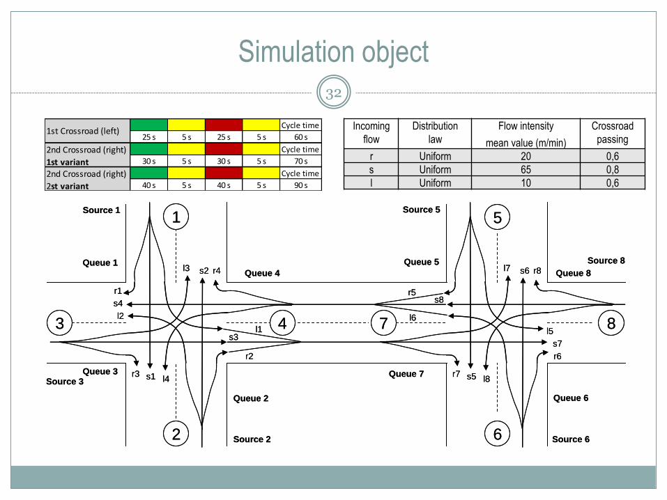
Simulation object32

Source 1

Source 2

r1

s1

l1

r2

s2

l2

r3

s3

l3 r4

s4

l4

Source 5

Source 6

r5

s5

l5

r6

s6

l6

r7

s7

l7 r8

s8

l8Source 3

1

2

3 4

Queue 4

Queue 7

7

Queue 2

Queue 3

Queue 1 Queue 5

Queue 6

Queue 8

Source 8

5

6

8

Source 1

Source 2

r1

s1

l1

r2

s2

l2

r3

s3

l3 r4

s4

l4

Source 5

Source 6

r5

s5

l5

r6

s6

l6

r7

s7

l7 r8

s8

l8Source 3

1

2

3 4

Queue 4

Queue 7

7

Queue 2

Queue 3

Queue 1 Queue 5

Queue 6

Queue 8

Source 8

5

6

8

Cycle time

25 s 5 s 25 s 5 s 60 s

Cycle time

30 s 5 s 30 s 5 s 70 s

Cycle time

40 s 5 s 40 s 5 s 90 s

1st Crossroad (left)

2nd Crossroad (right)

1st variant2nd Crossroad (right)

2st variant

Incoming

flow

Distribution

law

Flow intensity

mean value (m/min)

Crossroad

passing

r Uniform 20 0,6

s Uniform 65 0,8

l Uniform 10 0,6

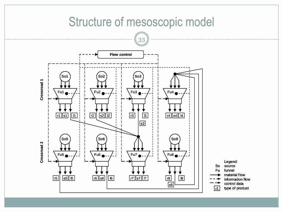
Structure of mesoscopic model33

So1

r1 s1 l1

So2 So3

Flow control

r2 s2 l2 r3

s3

l3 r4 s4 l4

Fu1 Fu2 Fu3 Fu4

Legend:

source

funnel

material f low

information flow

control data

type of productr1

So

Fu

So5

r5 s5 l5

So6 So8

r6 s6 l6 r7 s7 l7 r8

s8

l8

Fu5 Fu6 Fu7 Fu8

Cro

ss

road

1C

ross

road

2

So1So1

r1 s1 l1

So2So2 So3So3

Flow control

r2 s2 l2 r3

s3

l3 r4 s4 l4

Fu1 Fu2 Fu3 Fu4

Legend:

source

funnel

material f low

information flow

control data

type of productr1

So

Fu

Legend:

source

funnel

material f low

information flow

control data

type of productr1

So

Fu

So5So5

r5 s5 l5

So6So6 So8So8

r6 s6 l6 r7 s7 l7 r8

s8

l8

Fu5 Fu6 Fu7 Fu8

Cro

ss

road

1C

ross

road

2

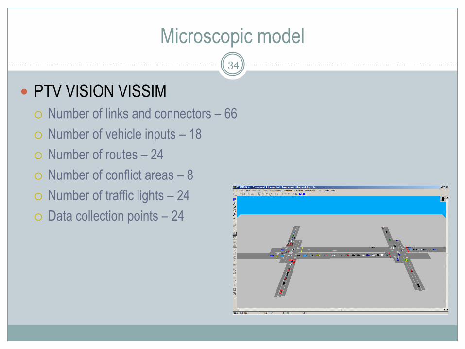
Microscopic model

PTV VISION VISSIM

Number of links and connectors – 66

Number of vehicle inputs – 18

Number of routes – 24

Number of conflict areas – 8

Number of traffic lights – 24

Data collection points – 24

34

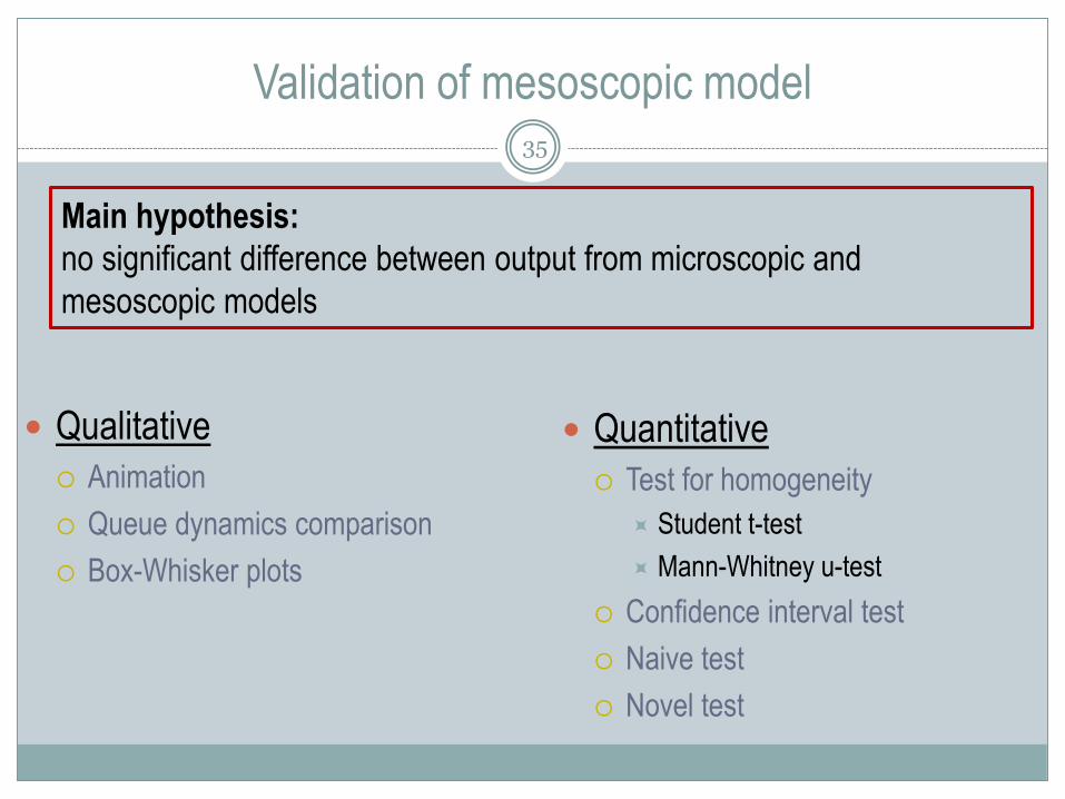
Validation of mesoscopic model

Qualitative

Animation

Queue dynamics comparison

Box-Whisker plots

35

Main hypothesis:

no significant difference between output from microscopic and

mesoscopic models

Quantitative

Test for homogeneity

Student t-test

Mann-Whitney u-test

Confidence interval test

Naive test

Novel test

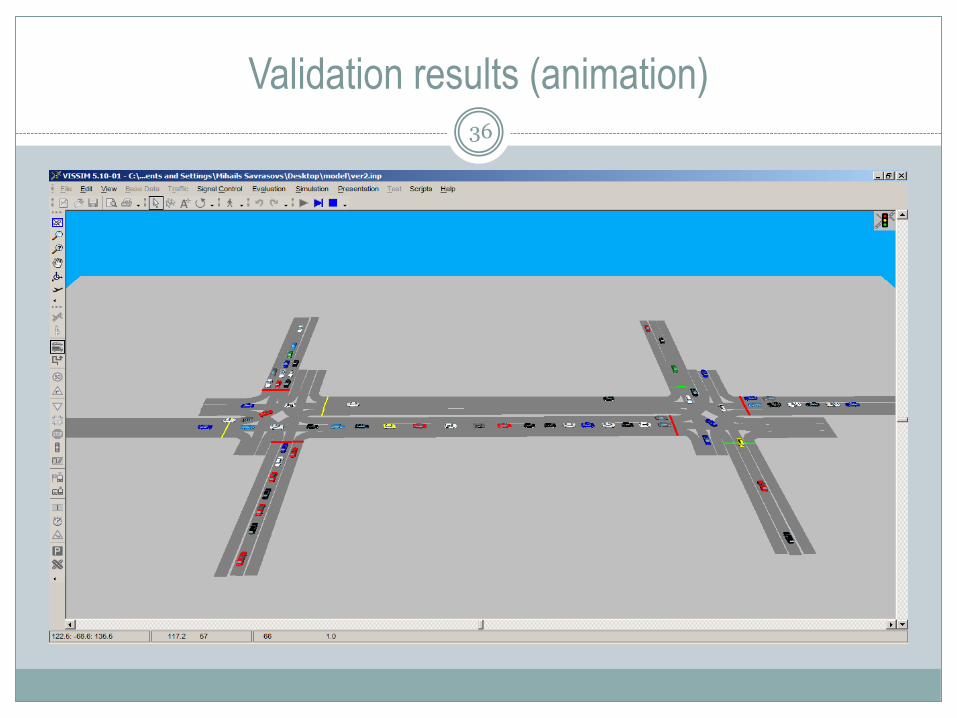
Validation results (animation)36

Validation results (queue dynamics comparison)37

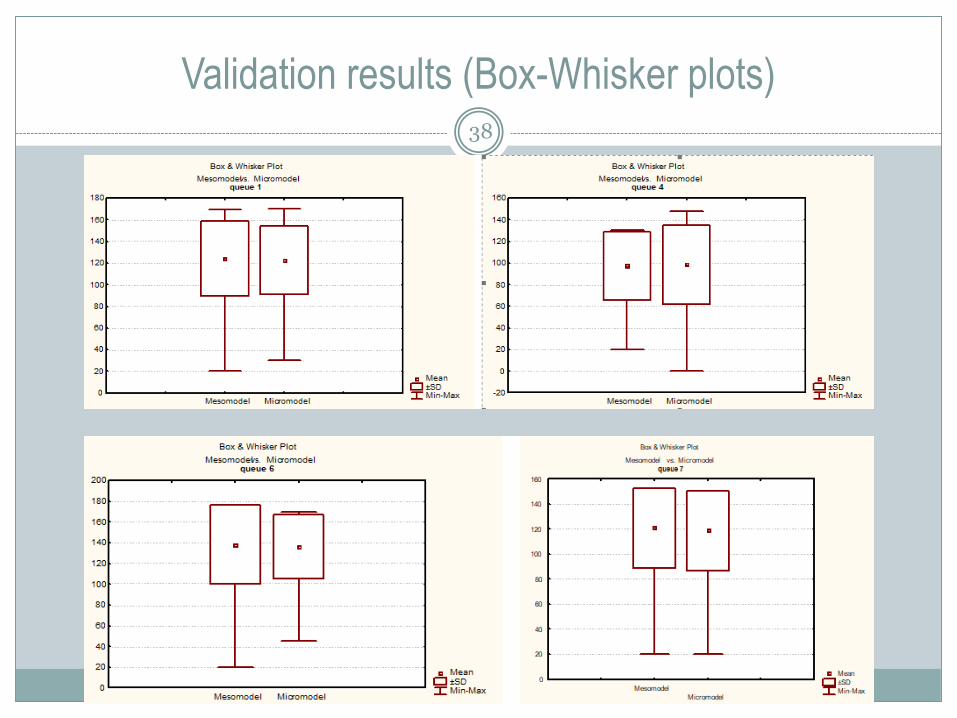
Validation results (Box-Whisker plots)38

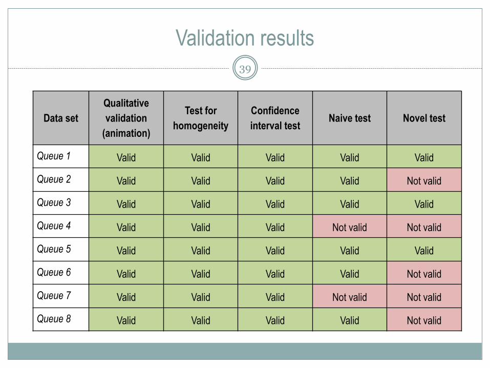
Validation results

Data set

Qualitative

validation

(animation)

Test for

homogeneity

Confidence

interval testNaive test Novel test

Queue 1 Valid Valid Valid Valid Valid

Queue 2 Valid Valid Valid Valid Not valid


Queue 4 Valid Valid Valid Not valid Not valid



Queue 7 Valid Valid Valid Not valid Not valid


39

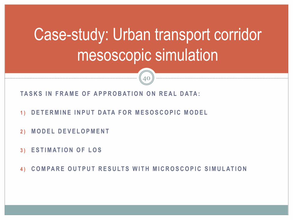
TA S K S I N F R A M E O F A P P R O B AT I O N O N R E A L D ATA :

1 ) D E T E R M I N E I N P U T D ATA F O R M E S O S C O P I C M O D E L

2 ) M O D E L D E V E L O P M E N T

3 ) E S T I M AT I O N O F L O S

4 ) C O M PA R E O U T P U T R E S U LT S W I T H M I C R O S C O P I C S I M U L AT I O N

40

Case-study: Urban transport corridor

mesoscopic simulation

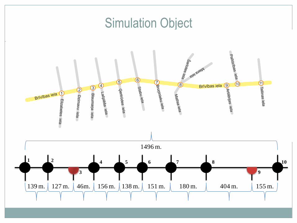
Simulation Object41

1496 m.

139 m. 127 m. 46m. 156 m. 138 m. 151 m. 180 m. 404 m. 155 m.

1 2

3

4 5 6 7 8

9

10

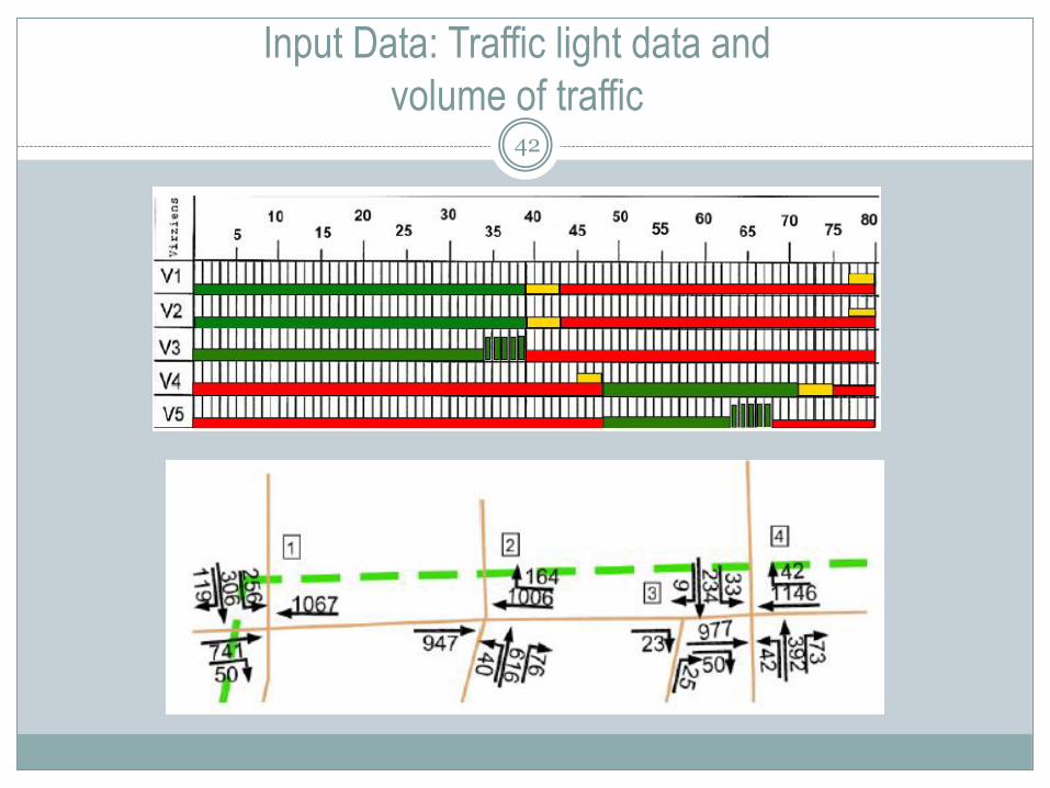
Input Data: Traffic light data and

volume of traffic42

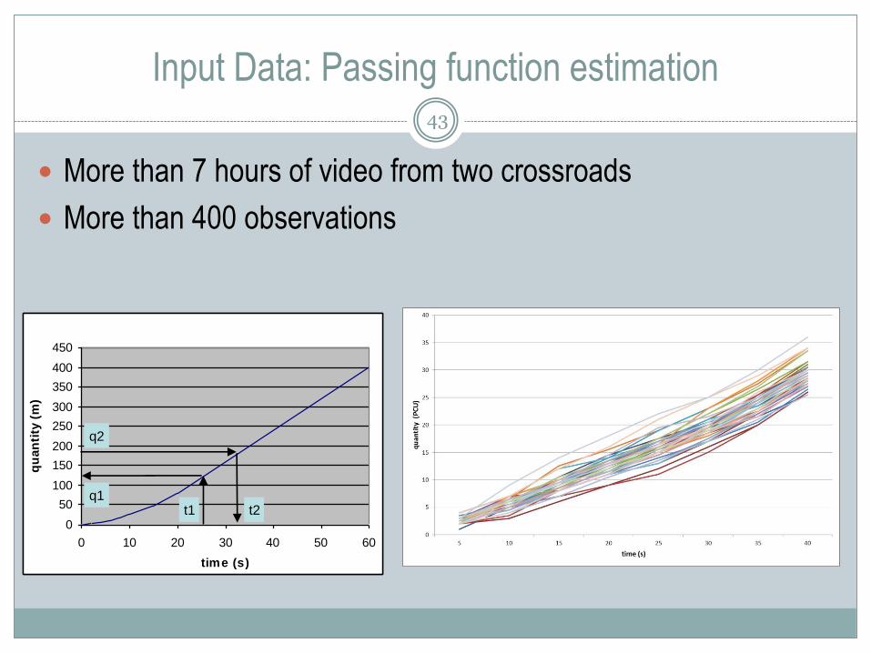
Input Data: Passing function estimation

More than 7 hours of video from two crossroads

More than 400 observations

43

Exemplary chart

0

50

100

150

200

250

300

350

400

450

0 10 20 30 40 50 60

time (s)

qu

an

tity

(m

)

t1 t2q1

q2

Exemplary chart

0

50

100

150

200

250

300

350

400

450

0 10 20 30 40 50 60

time (s)

qu

an

tity

(m

)

t1 t2q1

q2

ExtendSim simulation software47

https://www.extendsim.com

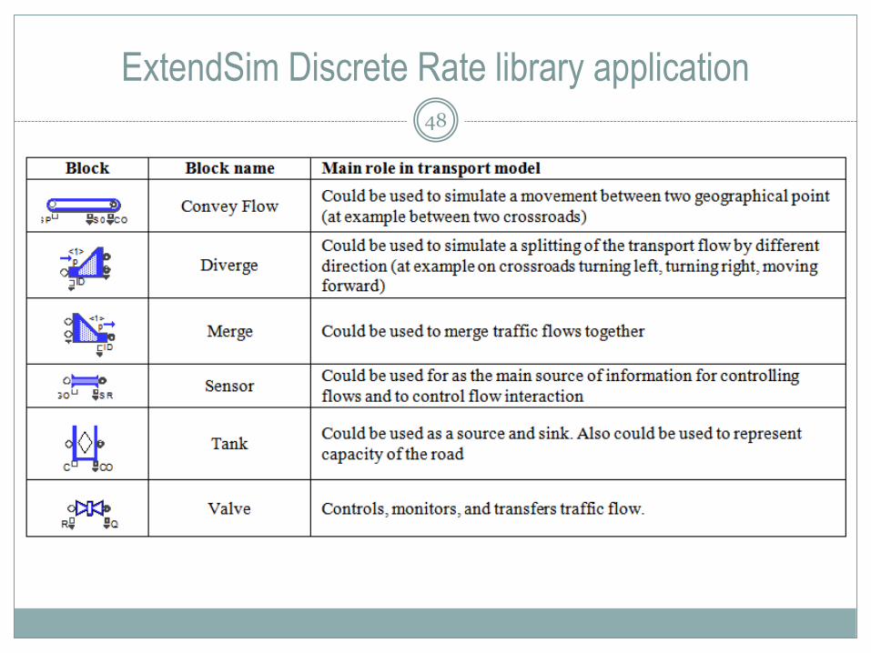
ExtendSim Discrete Rate library application48

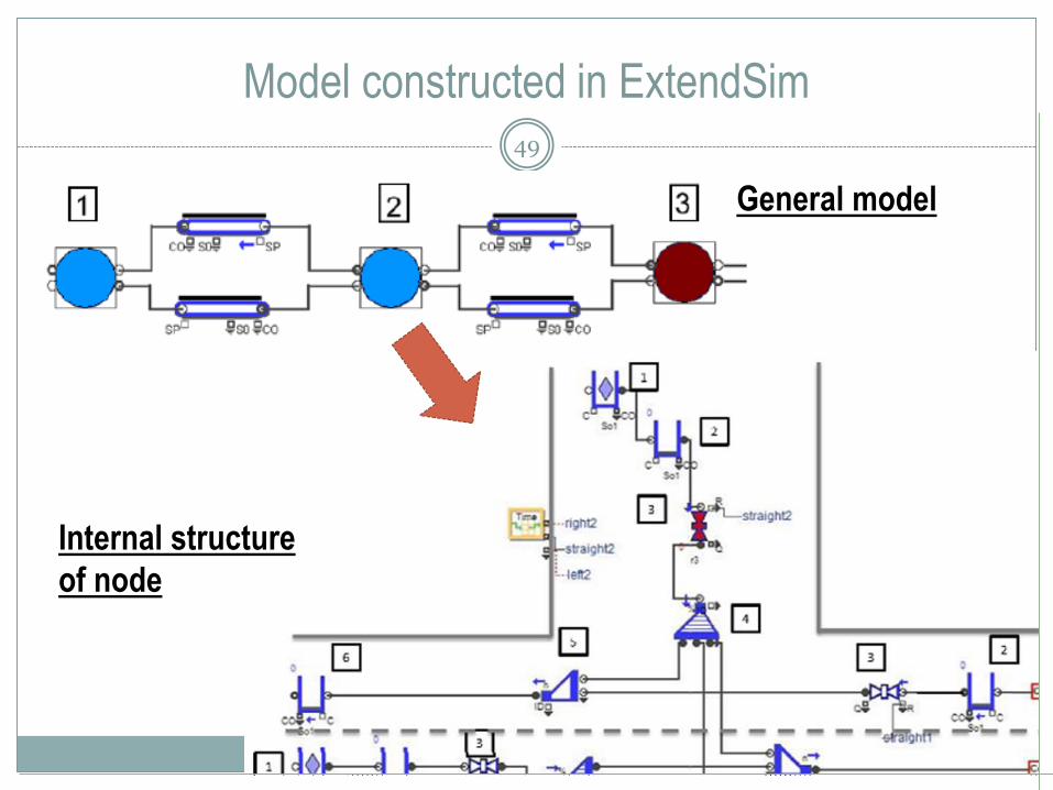
Model constructed in ExtendSim49

General model

Internal structure

of node

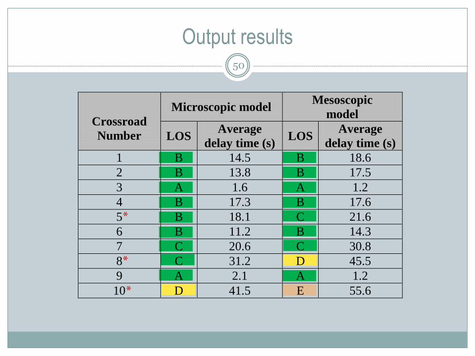
Output results50

Crossroad

Number

Microscopic model Mesoscopic

model

LOS Average

delay time (s) LOS

Average

delay time (s)

1 B 14.5 B 18.6

2 B 13.8 B 17.5

3 A 1.6 A 1.2

4 B 17.3 B 17.6

5 B 18.1 C 21.6

6 B 11.2 B 14.3

7 C 20.6 C 30.8

8 C 31.2 D 45.5

9 A 2.1 A 1.2

10 D 41.5 E 55.6

*

*

*

Mesoscopic vs Microscopic

(time resource)51

Publications (1/2)

Savrasovs M. "Traffic Flow Simulation on Discrete Rate Approach Base", Transport and

Telecommunication, Vol. 13, April, 2012, pp. 167-173.

Savrasovs M. “Urban Transport Corridor Mesoscopic Simulation”, the 25th European

Conference on Modelling and Simulation (ECMS’2011) , 2011, pp. 587-593.

Savrasovs M. “The Application of a Discrete Rate Approach to Traffic Flow Simulation”,

the 10th International Conference, Reliability and Statistics in Transportation and

Communication, 2010, pp. 433-439.

M. Savrasov, I. Yatskiv, A. Medvedev and E. Yurshevich. "Simulation as a Tool of

Decision Support Process: Latvia-based Case Study". In Proceedings of 1-st

International Conference on Road and Rail Infrastructure (CETRA 2010). 2010. pp.

217-222.

Savrasovs M. “Mesoscopic Simulation Concept for Transport Corridor”, the 12th World

Conference on Transport Research (WCTR 2010). Lisbon, Portugal, 2010.

52

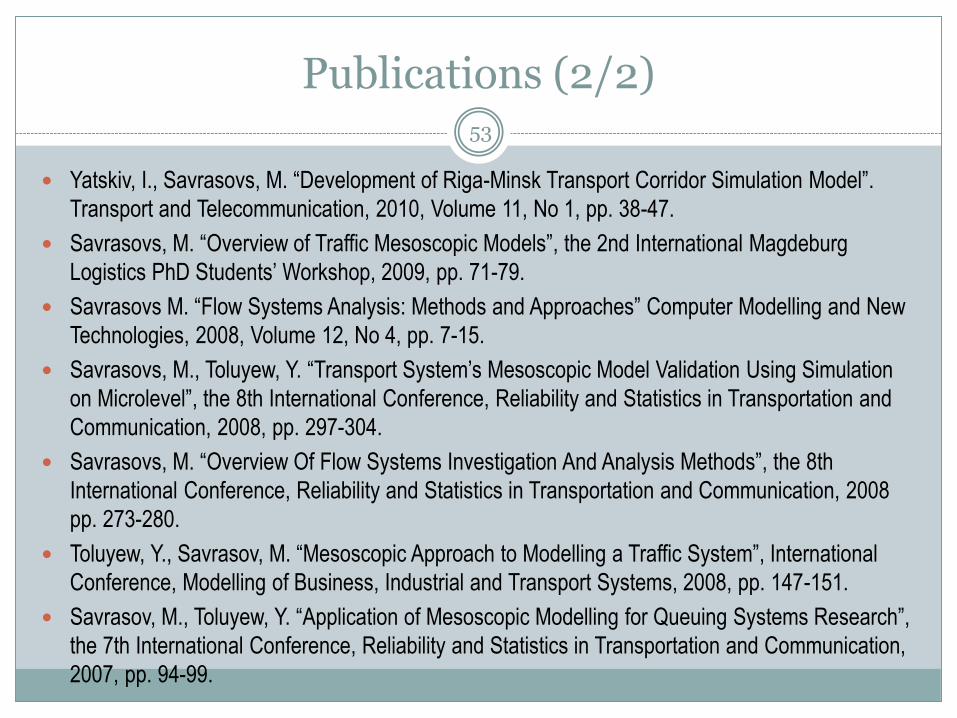
Publications (2/2)53

Yatskiv, I., Savrasovs, M. “Development of Riga-Minsk Transport Corridor Simulation Model”.

Transport and Telecommunication, 2010, Volume 11, No 1, pp. 38-47.

Savrasovs, M. “Overview of Traffic Mesoscopic Models”, the 2nd International Magdeburg

Logistics PhD Students’ Workshop, 2009, pp. 71-79.

Savrasovs M. “Flow Systems Analysis: Methods and Approaches” Computer Modelling and New

Technologies, 2008, Volume 12, No 4, pp. 7-15.

Savrasovs, M., Toluyew, Y. “Transport System’s Mesoscopic Model Validation Using Simulation

on Microlevel”, the 8th International Conference, Reliability and Statistics in Transportation and

Communication, 2008, pp. 297-304.

Savrasovs, M. “Overview Of Flow Systems Investigation And Analysis Methods”, the 8th

International Conference, Reliability and Statistics in Transportation and Communication, 2008

pp. 273-280.

Toluyew, Y., Savrasov, M. “Mesoscopic Approach to Modelling a Traffic System”, International

Conference, Modelling of Business, Industrial and Transport Systems, 2008, pp. 147-151.

Savrasov, M., Toluyew, Y. “Application of Mesoscopic Modelling for Queuing Systems Research”,

the 7th International Conference, Reliability and Statistics in Transportation and Communication,

2007, pp. 94-99.

traffic flows mesoscopic simulation...

Documents