data-driven mesoscopic simulation of large-scale surface ... · data-driven mesoscopic simulation...
TRANSCRIPT

Data-Driven Mesoscopic Simulation of Large-Scale Surface Transit Networks
by
Bo Wen Wen
A thesis submitted in conformity with the requirements for the degree of Master of Applied Science
Department of Civil Engineering University of Toronto
© Copyright by Bo Wen Wen 2017

ii
Data-Driven Mesoscopic Simulation of Large-Scale Surface
Transit Networks
Bo Wen Wen
Master of Applied Science
Department of Civil Engineering
University of Toronto
2017
Abstract
The planning of transit services, assessment of operational strategies, and evaluation of service
changes can benefit tremendously from high-fidelity transit network models. Traditional
microsimulation models are infeasible for large networks due to onerous model construction and
calibration and prohibitive computational requirements. They are typically only used to model
individual corridors or small sub-networks. This study presents a data-driven mesoscopic
simulation method that models surface transit movement based on open data and machine learning.
After a comprehensive comparison of running speed models using multiple linear regression,
support vector machine, linear mixed effect model, regression tree and random forest, the random
forest running speed models and lognormal dwell time distribution models were used to perform
stop-to-stop mesoscopic simulations. The model results adequately replicated variation in
headways, delays, and dwell times. Validation at the stop level and the route level demonstrated
the need to capture passenger demand and congestion variations in future studies.

iii
Acknowledgement
This research was made possible by the generous support of our industry research partner,
ARUP, as well as the grants and scholarships from the Natural Sciences and Engineering Research
Council of Canada.
I want to express my gratitude for Prof. Amer Shalaby’s supervision. His support,
guidance, and vision encouraged me to overcome many challenges. We have accomplished a great
deal together and I believe this thesis brings the transit research community closer to a world with
growing presence of data and artificial intelligence.
Thank you, Prof. Shoshanna Saxe, for providing valuable feedback on my thesis. I want to
also express gratitude for Siva Srikukenthiran’s efforts in making this project possible.
I want to thank the staff working at the Toronto Open Data Team for their efforts in making
quality transportation data available.
Special thanks to Kenny Ling from TTC for providing very valuable suggestions for
processing AVL data, you have saved me countless hours in figuring out the best way to structure
AVL data for analysis.
I am forever indebted to the open source developers for many of the R packages that I used
and the python packages I tested, as well as the countless number of posts that had taught me how
to code in C#, R, and Python on Stack Overflow.
Thank you to all the wonderful people working very hard with me along the way and cheer
me on day after day: Greg and Greg, Paula, Yishu, Ariel, Teddy, Sami, Adam, Nancy.
Finally, thank you to my family for supporting me and believing in me. My parents, Lina,
and David. Your love made everything possible in the most trying times.

iv
Table of Contents
List of Tables ................................................................................................................................ vii
List of Figures .............................................................................................................................. viii
Glossary ......................................................................................................................................... xi
Modelling Terms ....................................................................................................................... xi
Programming Terms................................................................................................................. xii
Chapter 1 Introduction ..............................................................................................................1
1.1 Thesis Objectives .................................................................................................................2
1.2 Surface Transit Modelling Approach ...................................................................................3
1.3 The Nexus Platform .............................................................................................................7
1.4 Thesis Outline ......................................................................................................................8
Chapter 2 Literature Review...................................................................................................10
2.1 Simulation Level of Detail .................................................................................................10
2.2 Simulation Models for Transit ...........................................................................................13
2.3 Statistical Learning Models ...............................................................................................16
2.4 Research Opportunities ......................................................................................................21
Chapter 3 Modelling Framework ...........................................................................................23
3.1 Functional Requirements ...................................................................................................23
3.2 Simulation Framework.......................................................................................................25
3.3 Detailed Functional Design................................................................................................28
3.4 Summary ............................................................................................................................35
Chapter 4 Data Collection ......................................................................................................36
4.1 Data Collection Methods ...................................................................................................36
4.2 Open Data Formats and Collections ..................................................................................39
4.3 Summary ............................................................................................................................50
v
Chapter 5 Data Processing ......................................................................................................51
5.1 Data Loading ......................................................................................................................52
5.2 Preprocessing of AVL data ................................................................................................57
5.3 AVL Trip Data Processing.................................................................................................61
5.4 Data Export ........................................................................................................................77
5.5 Summary ............................................................................................................................79
Chapter 6 Model Estimation ...................................................................................................80
6.1 Running Speed Model........................................................................................................81
6.2 Dwell Time Model ...........................................................................................................112
6.3 Summary ..........................................................................................................................115
Chapter 7 Simulation Procedures .........................................................................................116
7.1 Load Trained Models .......................................................................................................117
7.2 Initialize Simulation Data ................................................................................................118
7.3 Iterative Predictions .........................................................................................................119
7.4 Simulation Result Outputs ...............................................................................................122
7.5 Analytic Reports ..............................................................................................................126
7.6 Summary ..........................................................................................................................129
Chapter 8 Results of Case Study ..........................................................................................130
8.1 Case Study Background ...................................................................................................130
8.2 Summary of Data .............................................................................................................132
8.3 Running Speed Model......................................................................................................135
8.4 Dwell Time Distribution Model Result ...........................................................................140
8.5 Simulation with Random Forest ......................................................................................147
8.6 Simulation with Linear Mixed Effect Model ...................................................................152
8.7 Summary ..........................................................................................................................157
Chapter 9 Conclusion ...........................................................................................................158

vi
9.1 Summary of Results .........................................................................................................158
9.2 Research Contributions ....................................................................................................162
9.3 Future Research ...............................................................................................................163
Bibliography ................................................................................................................................164
Appendix A Selected Programming Code ................................................................................177
A.1 Data Collection Algorithm ...............................................................................................177
A.2 Data Processing Algorithm ..............................................................................................203
A.3 Model Estimation Algorithm ...........................................................................................277
A.4 Model Simulation Algorithm ...........................................................................................293
A.5 Analytic Report Algorithm ..............................................................................................301
Appendix B Software Repository.............................................................................................315
Appendix C TRB Paper 2016 ...................................................................................................316
Appendix D TransitData 2017 Abstract ...................................................................................337
vii
List of Tables
Table 1. Fields for GTFS CSV files.............................................................................................. 41
Table 2. Vehicle object fields for NextBus AVL XML files ........................................................ 44
Table 3. Closure object fields for Road Restriction XML files .................................................... 45
Table 4. Objects and fields in weather JSON files ....................................................................... 47
Table 5. Processed GTFS Database table information ................................................................. 53
Table 6. List of possible variables, attributes, by data sources ..................................................... 78
Table 7. Variables for route level basic model ............................................................................. 83
Table 8. Variables for network level advanced model analysis .................................................... 84
Table 9. Comparing linear and RBF kernels for support vector machine .................................... 94
Table 10. Random forest performances with increasing number of trees .................................. 107
Table 11. A sample of simulated and scheduled trip summary data .......................................... 124
Table 12. A sample of observed trip summary data from test data set ....................................... 125
Table 13. Detailed summary of open data sources ..................................................................... 134
Table 14. Comparison of route-level running speed models for 34-Eglinton East .................... 136
Table 15. Comparison of route-level running speed models for 54-Lawrence East .................. 137
Table 16. Comparison of route-level running speed models for 504-King ................................ 137
Table 17. Comparison of route-level running speed models for 512-St. Clair ........................... 138
Table 18. Comparison of five types of network-level running speed models ............................ 139
viii
List of Figures
Figure 1. Nexus simulation platform .............................................................................................. 8
Figure 2. Nexus surface simulator automatic modelling pipeline framework design .................. 27
Figure 3. Classes and data object references within the surface transit simulator tool ................ 30
Figure 4. Functional component calls within the surface transit simulator tool ........................... 34
Figure 5. Data collection for archival data .................................................................................... 37
Figure 6. Data collection for real-time online API data................................................................ 39
Figure 7. Data tool objects of the surface transit simulator .......................................................... 40
Figure 8. Data Processing Flow .................................................................................................... 51
Figure 9. Data points that cannot be used to produce trips, left: points with default location, right:
points in trip with no path travelled .............................................................................................. 58
Figure 10. Non-revenue trip for AVL points labelled as King Street shuttle bus ........................ 59
Figure 11. Multiple eastbound and westbound trips (over 10) on St Clair had the same trip
information, labelled as St Clair shuttle bus ................................................................................. 60
Figure 12. Trip forming using SQL database query, top: TTCGPS table containing AVL GPS
points, bottom: TTCGPSTRIPS table containing AVL trips........................................................ 62
Figure 13. Stop sequence trimming to delete stops not traversed by the observed trip ................ 65
Figure 14. Arrival and dwell time determination for a sample AVL trip ..................................... 66
Figure 15. Delay determination for all previous stop times served .............................................. 67
Figure 16. Delay determination for a trip with missed scheduled arrival times ........................... 69
Figure 17. Delay determination for a trip following the trip with missed arrival times ............... 69

ix
Figure 18. Headway determination demonstration ....................................................................... 70
Figure 19. Generation of link data using trip data ........................................................................ 73
Figure 20. Model estimation process flow for running speed model ........................................... 81
Figure 21. Separating and classifying data with support vector machine..................................... 90
Figure 22. Clustering pattern for links for route number 192 ....................................................... 98
Figure 23. Clustering pattern for links for route number 504 ....................................................... 99
Figure 24. Clustering pattern for links for route number 196 ....................................................... 99
Figure 25. Clustering pattern for links for route number 510 ..................................................... 100
Figure 26. Diagram of a simple regression tree model ............................................................... 102
Figure 27. Relative error of regression tree with increasing number of splits ............................ 102
Figure 28. Illustration of a random forest (R. Hänsch & O. Hellwich, 2015) ............................ 105
Figure 29. RMSE decreases and training time increases with increasing number of trees ........ 107
Figure 30. Model estimation process flow for dwell time model ............................................... 113
Figure 31. Simulation procedure process flow ........................................................................... 116
Figure 32. Flowchart of model simulation procedure ................................................................. 120
Figure 33. An example of time-distance diagram for Route 192 Airport Rocket NB ................ 127
Figure 34. Examples of route speed histograms for Route 192 Airport Rocket NB .................. 128
Figure 35. Examples of stop delay distribution curve ................................................................ 129
Figure 36. The Toronto Transit Commission downtown network map (Toronto Transit
Commission, 2017c) ................................................................................................................... 131
Figure 37. Dwell time model parameters at stops on coloured bubble map ............................... 142
x
Figure 38. Observed dwell times at stops on coloured bubble map ........................................... 144
Figure 39. Predicted dwell times at stops on coloured bubble map ............................................ 145
Figure 40. Chi-square goodness of fit test for dwell time predictions ........................................ 146
Figure 41. Time distance diagrams, 504 King WB and EB, for scheduled, observed and
simulated trips, simulated using Random Forest running speed model ...................................... 148
Figure 42. Route speed validation for four major TTC routes, simulated using Random Forest
running speed model ................................................................................................................... 149
Figure 43. Stop delay validation for four routes at 14 major TTC transfer stops, simulated using
Random Forest running speed model ......................................................................................... 151
Figure 44. Time distance diagrams, 504 King WB and EB, for schedule, observed and simulated
trips, simulated using Linear Mixed Effects running speed model ............................................ 153
Figure 45. Route speed validation for four major TTC routes, simulated using Linear Mixed
Effects running speed model ....................................................................................................... 154
Figure 46. Stop delay validation for four routes at 14 major TTC transfer stops, simulated using
Linear Mixed Effects running speed model ................................................................................ 156

xi
Glossary
Modelling Terms
• ROW: right of way in transit describes the area which transit vehicles pass through.
• Dedicated ROW: area which only transit vehicles may pass through
• Shared ROW: a shared area of road both transit vehicles and other vehicles may occupy
• Streetcar: light rail public vehicles on streets
• Subway: heavy underground rail vehicles
• AVL: automatic vehicle location systems which determine the locations of vehicles
• GTFS: General Transit Feed Specification is a common format for public transportation
schedules. It contains geographical information regarding each transit trip and schedule.
(Google Inc., 2016)
• Transit Trip: a sequence of stops along a route that occur at specific times (Google Inc.,
2016).
• Transit Route: a group of trips organized as a single service (Google Inc., 2016).
• Transit Stop: locations where transit vehicles board or alight passengers (Google Inc.,
2016).
• Vehicle Block: the complete itinerary of a transit vehicle for one day, including revenue
and non-revenue trips. Vehicle blocks in the context of GTFS data include only the revenue
trips since the GTFS schedules do not contain non-revenue trip information (Google Inc.,
2016).
• GTFS Shapes: lines with a sequence of geographical location data to represent transit
routes on a map (Google Inc., 2016).
xii
Programming Terms
• API: application programming interface is a set of clearly defined methods of
communications between software components.
• Web APIs: an interface that use Hypertext Transfer Protocol (HTTP) request messages to
retrieve response messages. Common response message formats are XML, JSON, and
CSV.
• CSV: comma-separated value format is a commonly used data storage format for tables of
values where column values are separated by a comma and rows are separated by newlines.
• XML: Extensible Markup Language is a language that defines a set of encoding rules for
documents in a way that is both human-readable and machine-readable. A key
characteristic of the XML format is the use of begin tag <aTag> and end tag </aTag>.
• JSON: JavaScript Object Notation is a data object transmission standard popularized by
JavaScript, which is both human-readable and machine-readable. A key characteristic of
the JSON format is the use of curly brackets and colons to define objects.
• Database: a collection of data organized for fast access by an application. It usually
contains a set of tables with defined data columns.
• Database Table: a matrix of related data with defined data columns and data types. Often,
a key can be defined for a table column for fast data row retrieval. Properties such as unique
or default values can be defined for convenient data insertions.
• SQL: refers to the programming languages that execute commands on a database table.
Some common SQL queries include: Create, Drop, Insert, Select, Update, and Vacuum.
• SQLite: a variant of SQL application that is optimized for file-based database operations;
in particular, it does not require a separate client-server process.
• File: a collection of data stored, usually on disk. A file may store data in different formats,
such as binary, text, CSV, JSON, XML, etc.

xiii
• Memory: a short-term, volatile data storage medium.
• Disk: a long-term, non-volatile data storage device.
• Data Type: a type of data can be primitives, such as string (text), int (integer), long (large
integer), double (decimal numbers), etc. It may also be complex data types that contain
many of data types defined within a class.
• Class: an extensible program code for creating objects. It defines the data types as well as
procedures within the class.
• Method: detailed instructions to perform a certain procedure.
• Data Object: an in-process object containing data of a specific data or class type.
• List: a type of object that contains many items of the same data type.
• Dictionary: a type of object that contains values of many items of the same data type, with
each item having a key that can be used for locating the item.

1
Chapter 1
Introduction
In an era when cities are growing at an ever-increasing rate while infrastructural
improvements are lagging, transit agencies are faced with difficulties in maintaining service
reliability in the face of chronic congestion. The ability to maintain service reliability is even more
difficult for routes running at capacity with short headways, giving transit agencies few options to
recover from heavy congestion and long delays. Furthermore, these delays from surface transit can
cause irregular crowding at major stations, spreading the effects of surface disruptions to other
parts of the transit network such as transit stations, as well as subway and rail systems. Currently,
transit agencies handle these service disruptions and irregularities in an ad-hoc fashion. This is
partly due to a lack of analytical tools to model and analyse network-level impacts of response
strategies. As such, the cascading effects of delays due to surface transit congestion on a
multimodal transit network are rarely quantified and thus poorly addressed. The difficulty of
operating reliable transit service in a congested network is evident for the Toronto Transit
Commissions network. According to TTC’s performance scorecard for May of 2017, only 58.4%
of the streetcars and 75.7% of the buses departed on-time, falling short of the 90% target TTC had
set for itself (Toronto Transit Commission, 2017a).
Microsimulation models are commonly used to assess transit operational performance on
a few selected routes. However, when the impact of policy decisions and strategies need to be
evaluated at the network level, microsimulation models are too resource intensive to build and
computationally intensive to calibrate (Casas, Perarnau, & Torday, 2011). Calculation of vehicle
trajectories using car-following models become intractable when the network is large and
congested. A new method of simulation is needed for the evaluation of large-scale transit networks.
The adoption of modern transit technologies such as automatic vehicle location (AVL),
automatic passenger counter (APC), and automatic fare collection (AFC) systems provides transit
agencies with a large quantity of data and the opportunity to develop data-driven transit models
(Wilson, 2016). Existing transit simulation models have a primary focus on characterizing the
2
passenger demand using survey data and AFC data with the assumption that all transit vehicles
operate according to schedule (Gaudette, Chapleau, & Spurr, 2016; Kucirek, 2012; Weiss,
Mahmoud, Kucirek, & Habib, 2014). Based on TTC’s performance score, running transit services
to schedule in a congested network such as Toronto is very difficult to achieve (Toronto Transit
Commission, 2017a). As such, many other studies account for the various effects that influence
transit travel times using machine learning models in real-time bus arrival prediction algorithms
(Bai, Peng, Lu, & Sun, 2015; X. Chen, Liu, Xia, & Chien, 2004; Elhenawy, Chen, & Rakha, 2014;
Farid, Christofa, & Paget-Seekins, 2016; Kormaksson, Barbosa, Vieira, & Zadrozny, 2014;
Rashidi, Ranjitkar, & Hadas, 2014; Shalaby & Farhan, 2004; Yu, Yang, & Yao, 2006). These bus
travel time prediction techniques are capable of representing the stochastic behavior of transit
travel times in a congested network. However, they have not previously been applied in a large-
scale transit simulation application.
This study presents an innovative approach to model transit vehicle movement using open
data sources and machine learning algorithms. This approach extracts and combines various data
sources, trains statistical models, and simulates surface transit movement. More importantly, data-
driven models can be trained on recent data to more accurately represent the various impacts on
transit operations. Data-driven transit simulation models such as the one presented in this thesis
can help transit agencies evaluate their operational strategies and plans using the data produced by
modern transit technologies.
1.1 Thesis Objectives
The primary objective of this thesis is to model and simulate transit vehicle movements for
large-scale networks accurately and efficiently, utilizing big data and open data. In particular, the
aim of this thesis is to identify and evaluate appropriate methods for travel time and dwell time
models, which would characterize the mesoscopic transit vehicle movements under dynamic
operating conditions. This type of modelling technique would allow for assessment of transit
operational performance at the network level. By utilizing open data, these models can be quickly
updated for real-time decision support. A secondary objective of the data-driven mesoscopic transit
simulator is to integrate with multimodal simulation platforms to assess network level impacts
3
across different modes of public transport. These objectives can be achieved by developing the
surface simulator as a modular automatic modelling pipeline with the use of open source machine
learning software packages. This thesis demonstrates the capability of the simulator to replicate
surface transit movements for the Toronto Transit Commission network.
1.2 Surface Transit Modelling Approach
An appropriate modelling approach was developed to achieve the study objectives. This
thesis uses multiple sources of open data and open-source statistical models to identify the factors
influencing transit movements. These factors were used to develop the transit model, which was
then used as the engine to perform surface transit simulation.
1.2.1 Open Data and Big Data
Recent progress in public transit network modelling has been made possible using
automatic data collection systems (ADCS), general transit feed specification (GTFS), and other
transportation-related open data such as weather, road restriction and traffic intersection data. The
advances in public transit data have enabled the use of statistical learning methods that require
large quantities of data.
ADCS, including automatic vehicle location systems (AVL), automatic passenger counting
systems (APC), and automatic fare collection systems (AFC), are capable of collecting real-time
data and archiving historical data (Wilson, 2016). Bus locations collected by AVL-based GPS data
are readily available in real time, and a large sample of this data can be collected at a lower
marginal cost by the ADCS. Then, bus location data can be used to model transit vehicle speed. If
available at the network level, APC and AFC data can be valuable in modelling passenger demand
and enable more realistic representation of passenger movements across a transit network. The
AVL bus location data is sufficient in determining the travel speed of vehicles along a transit route;
however, to quantify the effects of various factors on transit travel speeds, additional open data
sources are required.
4
To fully uncover the wealth of transit travel patterns from AVL data and enable their use
beyond descriptive statistics, key transit operational characteristics must be identified using transit
schedules. GTFS is a standardized open data format for transit schedule data (Goldstein & Dyson,
2013). GTFS data contains trip, schedule, route, and stop information, for the entire transit
network. Using the GTFS transit schedule data, the AVL bus location data of a route can be
matched to its GTFS schedule data. This enables the computation of many transit operational
characteristics, including stop times at all the stops along the route, headways at stops, and delays
at stops.
To understand the effects of additional factors such as weather, road restrictions, and
attributes of traffic intersections on transit movements, additional transportation-related data
sources must be matched to the AVL data to identify the effects of these additional factors on
transit movements. This thesis uses weather data, road restriction data, and traffic intersection to
identify numerous link characterises and route characteristics that can impact transit movements.
By incorporating additional open data sources, the policy-relevant factors affecting surface transit
travel times can be assessed: the number of signalized intersections, the number of vehicular turns,
the presence of dedicated transit lane, the presence of transit signal priority, and transit stop
locations. This allows the model to assess the degree of impact policy changes can have on transit
performances. A policy sensitive model can be produced using the additional factors from open
data.
1.2.2 Link Representation
The method used for data processing is affected by how transit movements are represented
and thus a consistent link representation need to be established early on in this study. To represent
transit movement, a model incorporating both the transit running speed and dwell times need to be
captured (Padmanaban, Vanajakshi, & Subramanian, 2009). Because running speed and dwell time
of a transit vehicle are associated with the transit link the vehicle is traversing, an accurate
modelling of transit speeds and travel times requires a consistent representation of the link. There
are a few options available for representing links: by terminal stations, by time points, and by
stops.

5
Terminal-station-based segments, or route level segments provides better prediction
accuracy of average speeds over stop-based segments due to higher variations of speed observed
within shorter length of links (W. X. Hu & Shalaby, 2017). However, route level segments are not
suitable for this study because they cannot provide arrival patterns at major subway stations for
transit lines that do not terminate at these stations (M. Chen, Yu, Zhang, & Guo, 2009). The ability
to generate transit vehicle arrival patterns at major subways stations is important for this study.
Time-point-based segments can be a suitable approach and were used by many previous
studies (X. Chen et al., 2004; Yu et al., 2006). However, time points are generally not marked in
GTFS schedule data and the determination of time points are not standardized across transit
agencies (City of Toronto, 2017a). This makes time-point based segments difficult to implement
in a consistent way. In addition, the process of aggregating multiple stops into a single link can
exclude stops of interests. The possible exclusion of stops of interests can generate issues during
simulation when attempting to produce arrival patterns at key stations. With the exclusion of key
stops, it is difficult to assess of policies such as stop relocation, stop removal, and stop addition
since the many stop locations were aggregated as one time-point-based segment.
The use of stop-based links is not common in transit travel time studies since the
achievement of high model fitness and high accuracy can be difficult due to the higher degree of
random effects on travel time relative with shorter length of links (W. X. Hu & Shalaby, 2017).
However, there are several benefits with stop-based links. Firstly, stop-based links represent the
movement of transit vehicle between stops along an entire route. This provides greater simulation
fidelity. Secondly, the modelling of stop-based links enables detailed simulation of transit
passenger travel demand from origin to destination, when such information is available. Passenger
demand is an important aspect of transit models. Finally, stop-based link representations are
consistent with those used by standard transit schedule data such as GTFS. This allows for a
consistent mapping between GTFS schedule times and the calculated AVL stop times, which can
be advantageous in evaluating transit services at across stops and stations. This thesis will explore
the use of stop-based link representation for transit models.

6
1.2.3 Statistical Models for Transit Movements
With the goal of providing an accurate representation of transit travel patterns, structured
data obtained from various open data sources were used to estimate running speed and dwell time
models. To estimate these models, the unstructured data must first be processed into a list of
attributes that can be used as variables of the model – these are structured data. Once structured
data are obtained through data processing, the modelling methods for the running speed and dwell
time models were determined and evaluated.
In the field of machine learning, model accuracy, model training time, and model
prediction time are important criteria to assess to suitability of the method for modelling (Lim,
Loh, & Shih, 2000). Since this study uses various machine learning methods to model transit travel
times, model selection for this study will be based on a trade off between accurate representation,
training time, and simulation time. More complex modelling methods may allow more flexibility
in model representation and improve model fitness, but such flexibility can impose a heavier
computational cost in model training and in generating predictions for simulation (Caruana &
Niculescu-Mizil, 2006; Lim et al., 2000). Balancing these trade offs is important in producing
useful models, especially for application in large-scale networks.
While there are many previous studies on travel time models for transit vehicles, they
generally model up to several transit routes (Bai et al., 2015; X. Chen et al., 2004; Elhenawy et al.,
2014; Farid et al., 2016; Kormaksson et al., 2014; Rashidi et al., 2014; Shalaby & Farhan, 2004;
Yu et al., 2006). For the estimation of a large-scale transit running speed model involving a large
number of routes and trips, data clustering can become an issue since particular transit links and
route environments may have significant differences in running speed (Lee, Si, Chen, & Chen,
2012). An important aspect of this thesis is to properly characterize the data clustering effects on
running speeds due to link attributes. Providing an accurate representation of running speed with
feasible training time and efficient simulation method is critical to the simulation of surface transit
for Nexus.
1.2.4 Simulation Demonstration
Stop-based running speed and dwell time models were used as the engine to drive the
simulation of transit vehicles travelling across a series of transit links. To demonstrate the
7
capability of the surface transit simulation engine, all transit routes over the study period will be
simulated based on scheduled release of vehicles from the terminal station for the first trip of the
vehicle block. The simulation case study demonstrates the capabilities of data-driven transit
simulation models.
1.2.5 Toronto Transit Commission Case Study
The Toronto Transit Commission (TTC) bus and streetcar network was chosen to illustrate
the ability of large-scale transit statistical running speed and dwell times models with stop-based
link representation and the use of open data, to accurately represent the travel patterns of surface
transit vehicles. This study uses the TTC GTFS schedule data, TTC NextBus AVL real-time data,
Toronto intersection data, Toronto road restriction data, and Toronto weather data to characterize
the attributes and conditions of transit travel. The statistical models were evaluated on their ability
to predict running speeds and dwell times across the entire network for simulation purposes. The
variables used for the statistical models were based on the available open data sources and their
statistical significance; the statistical models can be extended in future studies. The framework
used in this study can be applied to other transit networks as well.
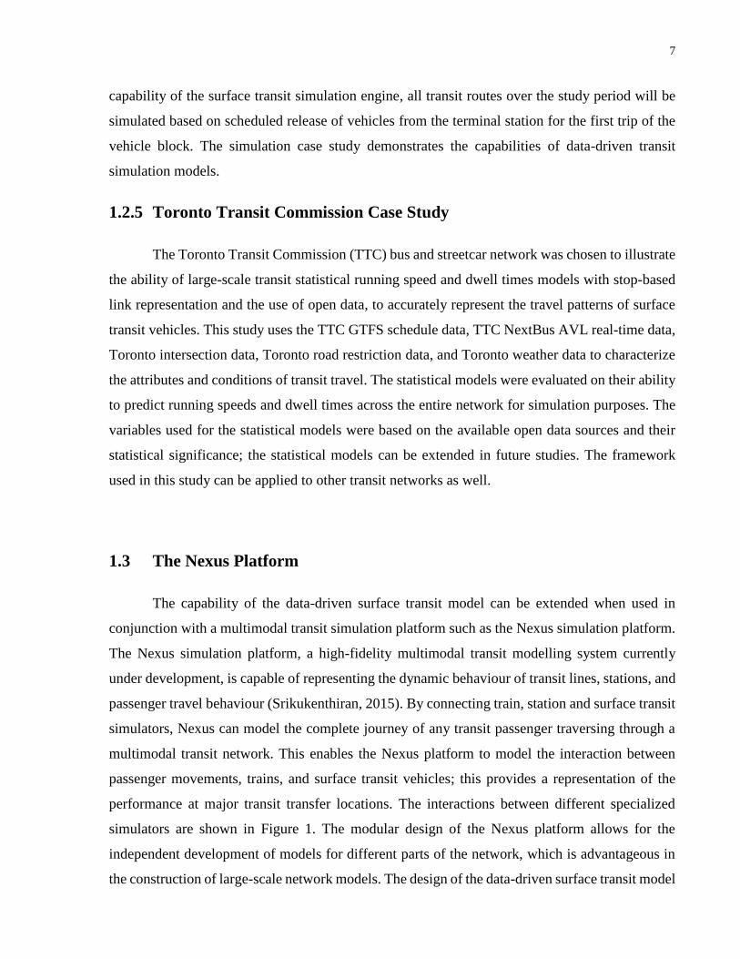
1.3 The Nexus Platform
The capability of the data-driven surface transit model can be extended when used in
conjunction with a multimodal transit simulation platform such as the Nexus simulation platform.
The Nexus simulation platform, a high-fidelity multimodal transit modelling system currently
under development, is capable of representing the dynamic behaviour of transit lines, stations, and
passenger travel behaviour (Srikukenthiran, 2015). By connecting train, station and surface transit
simulators, Nexus can model the complete journey of any transit passenger traversing through a
multimodal transit network. This enables the Nexus platform to model the interaction between
passenger movements, trains, and surface transit vehicles; this provides a representation of the
performance at major transit transfer locations. The interactions between different specialized
simulators are shown in Figure 1. The modular design of the Nexus platform allows for the
independent development of models for different parts of the network, which is advantageous in
the construction of large-scale network models. The design of the data-driven surface transit model
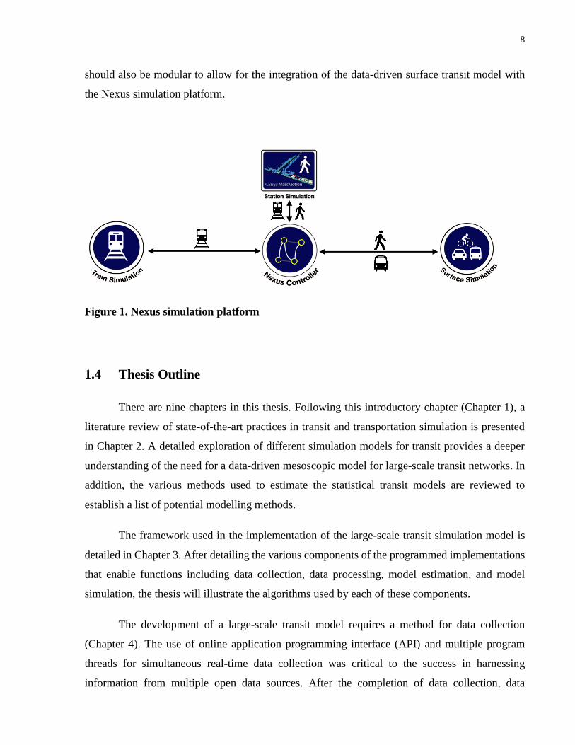
8
should also be modular to allow for the integration of the data-driven surface transit model with
the Nexus simulation platform.
Figure 1. Nexus simulation platform
1.4 Thesis Outline
There are nine chapters in this thesis. Following this introductory chapter (Chapter 1), a
literature review of state-of-the-art practices in transit and transportation simulation is presented
in Chapter 2. A detailed exploration of different simulation models for transit provides a deeper
understanding of the need for a data-driven mesoscopic model for large-scale transit networks. In
addition, the various methods used to estimate the statistical transit models are reviewed to
establish a list of potential modelling methods.
The framework used in the implementation of the large-scale transit simulation model is
detailed in Chapter 3. After detailing the various components of the programmed implementations
that enable functions including data collection, data processing, model estimation, and model
simulation, the thesis will illustrate the algorithms used by each of these components.
The development of a large-scale transit model requires a method for data collection
(Chapter 4). The use of online application programming interface (API) and multiple program
threads for simultaneous real-time data collection was critical to the success in harnessing
information from multiple open data sources. After the completion of data collection, data

9
processing of open data from real-time and archival sources enabled the fusion of multiple data
sources using spatiotemporal map matching techniques (Chapter 5).
Using the structured data obtained via data processing, several machine learning algorithms
were used to estimate and evaluate the potential statistical learning models (Chapter 6). The
recommended modelling method is based on the ability of the model to more accurately predict
the running speeds and dwell times of the vehicles across the transit network. To demonstrate the
implementation of the recommended models as the transit vehicle movement engine for simulation
applications, a procedure used to generate simulated trips based on a base case simulation scenario
was developed (Chapter 7). Lastly, the modelling and simulation demonstration results is
presented for a case study of the TTC network (Chapter 8). The case study demonstrates the
possible application of the statistical transit running speed and dwell time models for the Nexus
platform.
Finally, the final chapter provides a summary of the methods, results, and findings of the
thesis. The thesis ends with some suggestions of possible extensions to this study and establishes
potential future research directions (Chapter 9).
10
Chapter 2
Literature Review
The modeling and simulation of transit vehicles for large networks is a challenging task
due to its high computational requirements. Often, studies on transit modelling have focused on
isolated areas of networks where the factors affecting transit movement were specific to a limited
number of routes (Bai et al., 2015; Yu, Lam, & Tam, 2011). Since different transit modelling
approaches impose different computational requirements, selecting an appropriate modelling
method becomes critical to the success of the simulation framework when the network is large.
Therefore, an appropriate method for modelling must be chosen.
Expanding on the surface transit modelling approach we identified in the introduction, the
various methods used by previous studies are explored. Firstly, the trade-off between the level of
detail and computational requirements for traffic and transit modelling is discussed. Then, the
statistical methods used for transit travel time models are comprehensively reviewed. In addition,
the methods used by previous studies to model transit using open data such as GTFS and AVL
provide an in-depth understanding of the benefits of combining data sets to enhance models and
analyses. Finally, an appropriate method that addresses the modelling needs of a large-scale transit
network is presented.
2.1 Simulation Level of Detail
The level of detail required in simulation models depends on the nature of the research
study. There are three major types of simulation models as classified by the level of detail:
macroscopic, microscopic, and mesoscopic models. In the following sections, the abilities of
various simulations models to address research question at different level of modelling detail are
discussed.

11
2.1.1 Macroscopic Models
Macroscopic models describe traffic flow in aggregate variables such as flow, density and
speed and they include a lower number of parameters than microscopic models (Spiliopoulou,
Kontorinaki, Papageorgiou, & Kopelias, 2014). There are three main categories of previous studies
estimating traffic states: replicating traffic flow along congested freeway segments, using field
data and recursive filtering algorithms to dynamically adjust analytical traffic flow models, and
employing statistical or machine learning algorithm to generate short term predictions of traffic
states (Yang, Haghani, & Qiao, 2013). Similar to other models, macroscopic models require proper
calibration to generate realistic traffic states. Given the complex nature of transit systems,
particularly the interactions of traffic when it stops for passengers at different lanes and road
segments, macroscopic models are not as popular. More importantly, traditional macroscopic flow
models do not track the movements of individual vehicles and this limitation makes modelling of
transit movements difficult.
2.1.2 Microscopic Simulation Models
In contrast to macroscopic models, microscopic models simulate a high level of details
using detailed models such as the car-following models of traffic flow. Microscopic models can
simulate individual vehicles and their detailed movements. Previous studies demonstrated the
capabilities of microscopic simulation software, Paramics, in simulating various interactions
between transit vehicles, passengers, and traffic, such as bus holding, active transit signal priority
for buses, skip-stop operations, and bus station passenger transfers (Fernandez, Cortes, & Burgos,
2010). However, microscopic simulations’ vehicle routing algorithm suffer from a nonlinear
increase in computation requirements as network size increases (Cortés, Pagès, & Jayakrishnan,
2005). To overcome this limitation, mesoscopic simulation tools are used for vehicle route
decisions (Cortés et al., 2005). While microscopic simulation models generate a high level of
detail, calibration of large networks is very difficult and computation requirements can be
prohibitive.
12
2.1.3 Mesoscopic Simulation Models
While macroscopic models may lack a level of details required for transit modelling and
microscopic models may not be suitable for large-scale applications, mesoscopic models can be a
suitable alternative to fulfil both of these needs. Mesoscopic simulation models represent
individual vehicles but treat each roadway segment as queues and lanes are not represented
explicitly (Cats, Burghout, Toledo, & Koutsopoulos, 2010). One example of mesoscopic
simulation platform is Mezzo. Unlike microscopic simulation models, the links of Mezzo models
have a running part that contains vehicles not delayed by downstream and queueing part that
extends upstream from the end of the link when capacity is exceeded; the exit time of vehicles
entered the queue is calculated as a function of the density in the running part (Cats et al., 2010).
Mesoscopic models like Mezzo can simulate bus routes and collect stop-level statistics and are
suitable alternatives for large-scale applications.
2.1.4 Determining Simulation Level of Detail
The level of detail required in simulation models depends on the nature of the research
study. For instance, macroscopic models often address the relationships between flow, density and
speed but do not have the ability to trace individual vehicles (Spiliopoulou et al., 2014). In contrast,
microscopic simulation models based on the car-following model provides detailed vehicle
trajectories of all vehicles in the network at every time step but impose a higher computational
requirement (Cortés et al., 2005). Finally, mesoscopic simulation platform such as Mezzo uses a
queueing model to represent the movement of particular vehicles along transit links, balancing the
need to trace specific vehicles and computational requirements (Cats et al., 2010). The level of
detail of the models can impact computational requirements as well as the type of analysis that can
be performed. For studies interested in the capacity analysis of roadway and identifying traffic
bottlenecks, a macroscopic model is most suitable and most efficient. The capacity analysis of a
network may not be sufficient for studies requiring characterization of vehicle trajectories. In the
case of public transit modelling, microscopic simulation is preferred when computational
requirements are not a concern, such as for smaller networks (Cortés et al., 2005). However,
mesoscopic simulation may be desired if only a subset of vehicle trajectories must be determined,
such as in the case for large-scale transit simulations (Cats et al., 2010).

13
2.2 Simulation Models for Transit
As open data sources such as AVL, APC and AFC data become more readily available
from various transit agencies, a standard format was needed for transit data (Wilson, 2016). The
Google Transit Feed Specification (GTFS) common format enhances the interoperability of transit
data, thus allowing the development of applications using these data (Catala, Dowling, &
Hayward, 2011). In the following two sections, 2.2.1 and 2.2.2, the current state of the art in the
use of open data sources for transit simulation are discussed. These simulation models currently
place an emphasis on passenger demand modelling but do not model the stochastic travel time
behavior of surface transit vehicles, instead assuming transit vehicles proceed according to
schedule.
2.2.1 MATSim Model using GTFS and TTS
While GTFS data had previously been used to develop traveller information applications,
Kucirek has built a multimodal network model of the Greater Toronto and Hamilton Area (GTHA)
using GTFS data and Transportation Tomorrow Survey (TTS) data (Kucirek, 2012). The GTFS
data allowed Kucirek to construct scheduled vehicle trips. Kucirek used MATSim, a Java based
open-source simulation platform, to construct the simulation network based on GTFS data
(Kucirek, 2012). Kucirek converted an existing EMME2 model of the GTHA into the MATSim
network, creating the network nodes and links properties in the MATSim network (Kucirek, 2012).
More importantly, Kucirek used the semi-automated map-matching procedure developed by
Ordonez & Erath (Ordonez & Erath, 2011). A notable problem with Ordonez & Erath’s method is
the mismatch between the locations of GTFS bus stops and the simulation model’s bus stop. To
resolve this, Kucirek referenced multiple GTFS stops to a single geo-coded network link (Kucirek,
2012). Using the model constructed in MATSim, Kucirek could demonstrate the ability of
MATSim to be configured to include the effects of congestion in transit routing, and the ability of
MATSim to assign traffic and transit volumes (Kucirek, 2012).
Building upon Kucirek’s work on transit assignment, Weiss proposed a dynamic
multimodal assignment using a similar model and approach (Weiss et al., 2014). Using GTFS data
and TTS data, Weiss constructed a multimodal network with some improvements. Firstly, he

14
proposed additional solutions to the mismatched bus stop problem with Ordonez & Erath’s
method: increase the resolution of the simulation network to match that of GTFS data; and
removing stops to match the lower resolution of the simulation network (Weiss et al., 2014). This
results in a better definition of transit stops. He defined different types of GTFS stop clusters and
computed an equivalent multimodal network solution, accurately identifying different bus stop
types: transfer station, intersection stations and intermediate stops (Weiss et al., 2014).
Additionally, he reduced the size of the routing search space by proposing a more detailed
automated router network generation algorithm to consider more realistic transit transfers; this
reduced computation effort and generated more logical network routing results (Weiss et al.,
2014). Finally, Weiss noted a few issues with this assignment framework for the GTHA: use of
flat fare for all transit agencies generated unrealistically high assignments on some transit lines;
over prediction of traveller demands on specific stretches of highways with road pricing; and the
absent of multi-modal trip chaining behaviour in this model, particularly between modes (Weiss
et al., 2014).
2.2.2 MATSim Model using GTFS and Smart Card Data
Rather than using retrospective telephone survey data such as the TTS, Gaudette
demonstrated the use of a highly detailed public transit microsimulation model using GTFS and
tap-in smart card data from the Sociéte de transport de Laval (STL) bus network (Gaudette et al.,
2016). The use of smart card data allowed Gaudette to couple transit vehicle trips with passenger
actions; therefore, the passenger transfer behaviour can be represented (Gaudette et al., 2016).
Due to the moving fare box and lack of tap-out smart card data in Laval, determining the
exact boarding and alighting location of passengers was challenging. Gaudette used four methods
to match fare box transaction to boarding location: using subway station fare box as an anchor,
matching vehicle block, matching route-time window, and manual adjustments (Gaudette et al.,
2016). After the boarding location was determined, the trip was classified as a transfer from a
subway trip or initial boarding (Gaudette et al., 2016). For alighting location, the transaction
sequence of the smart card was used to determine where the user returned to the transit system;
however, if transaction sequence provides insufficient information, then a proportional distribution
calculation was used to determine the bus alighting locations (Gaudette et al., 2016).
15
The benefit of population level data sets such as the smart card data is that they allow for
accurate analysis of low-ridership lines for which insufficient samples exist for a conventional
survey such as the TTS. Gaudette validated the result of the model using APC data. However, trip
chaining between different modes, such as park and ride or kiss and ride, was still not captured.
Further research is needed to enrich data sources to provide true origin and destination points
(Gaudette et al., 2016).
2.2.3 Limitations of Simulation Models
Simulation models have been the standard of practice for assessing traffic congestion and
transit operation since they provide a way for researchers to perform scenario analysis without the
need to run a controlled experiment in real life (Weiss et al., 2014). The reliability of these models
depends on the careful calibration of several components of the models such as travel demand
models (generation of the origin-destination matrix), traffic and transit assignment models, mode
choice models, and car-following models or queueing models. The calibration of these various
models within the simulation model can be difficult and requires an extensive and expensive
survey (Kucirek, 2012).
As such, recent transit simulation models have advanced with the use of GTFS, smart cards
and APC data. These microscopic models rely heavily on the assumption of on-time transit vehicle
operations. As a result, they lack the stochastic representation of transit travel times due to the
effects of temporal variation, roadway incidents, weather, route characteristics, and link
characteristics. The primary focus of existing transit simulation models has been on passenger
demand and transit assignments; however, surface vehicle movement needs to be characterized in
order to determine passenger boarding and alighting at major transfer stations (Gaudette et al.,
2016). One of the key objectives of this thesis is to provide an accurate and efficient representation
of surface transit travel times across the entire transit network using existing data. Statistical
learning methods provide a means of achieving this goal. As such, various statistical learning
models for characterizing transit travel times are investigated in the following section.

16
2.3 Statistical Learning Models
With the advent of the global positioning system (GPS) based automatic vehicle location
(AVL) system, automatic passenger counter (APC) and other intelligent transportation systems
(ITS) for transit vehicles, statistical models including those based on machine learning algorithms
have been used by many previous studies for bus-arrival time and travel time prediction models
(Bai et al., 2015; X. Chen et al., 2004; Elhenawy et al., 2014; Farid et al., 2016; Kormaksson et
al., 2014; Rashidi et al., 2014; Shalaby & Farhan, 2004; Yu et al., 2006). These regression models
provide travel time predictions between stops and dwell times at stops and can be a
computationally efficient way to characterize the various effects on transit travel times. However,
they have not previously been applied in the setting of large-scale transit simulation, as is
performed in this thesis. In the following sections, 2.3.1 to 2.3.7, various modelling methods are
reviewed to form an understanding of existing state of the art statistical learning models for transit
travel time models. The limitations of each model in previous studies are assessed to determine
appropriate statistical learning models for use in this thesis.
2.3.1 Multiple Linear Regression
Multiple linear regression is one of the most commonly used regression models in research
as it reveals the degree of importance of independent variables (Bai et al., 2015). Using a linear
combination of independent predictor variables, multiple linear regression estimates the
coefficients of predictor variables by minimizing the variances. Multiple linear regression does
this based on the fundamental assumptions of linearity, independence, normal errors, and
homoscedasticity (Marill, 2004). Early studies on bus travel time used multiple linear regression
to assess travel time and reliability on arterial roads (Polus, 1979). Later studies on bus travel time
compared multiple linear regression to other regression models such as artificial neural networks
and support vector machine (Bai et al., 2015; Jeong & Rilett, 2004). In this study, multiple linear
regression was used as the basis for model comparison when evaluating more advanced regression
models.

17
2.3.2 Linear Mixed Effects Models
Another class of statistical model used for travel time prediction is linear mixed effects
model. Unlike most fixed-effects only models such as multiple linear regression, mixed effects
model deals with heteroscedasticity by accounting for correlations due to a grouping of subjects
or repeated measurements on each subject using random effects parameters (Seltman, 2016). A
varying intercept linear mixed effects model has been used for a travel time prediction model for
four regional bus routes in Rio Janeiro (Kormaksson et al., 2014). This study found the addition
of a random intercept for each bus ride improved model fitness by correcting the interpolating
errors due to repeated measurements per each bus trip (Kormaksson et al., 2014). Linear mixed
effects model can be useful in modelling variables with random effects due to repeated sampling.
2.3.3 Kalman Filter Algorithm
Instead of modelling effects of many explanatory variables on a predictor variable, the
Kalman filter algorithm models the recursive states of a predictor variable across time (Harvey,
1990). The Kalman filter is a process model that represents cyclic patterns between variables; it is
estimated using a linear recursive predictive update algorithm (Shalaby & Farhan, 2004). A bus
arrival and departure time prediction model for bus route number 5 in downtown Toronto had been
developed using Kalman filter (Shalaby & Farhan, 2004). The running time and dwell time models
used the Kalman filter algorithm, as well as Automatic Vehicle Location (AVL) and Automatic
Passenger Count (APC) data (Shalaby & Farhan, 2004). The model successfully captured the
interaction between running times and dwell times; also, it outperformed the predictive ability of
multiple linear regression and neural network models against real-world data (Shalaby & Farhan,
2004). Since the Kalman filter algorithm is designed to be updated in real-time during model run
time, it is commonly used for real-time travel time prediction application rather than offline transit
planning purposes.
2.3.4 Artificial Neural Network
The modelling of the recursive states of travel time using Kalman filter may not sufficiently
capture various effects on travel time. A study using weather and APC data for New Jersey Transit
route number 62 was conducted to demonstrate the use of both Kalman filter and artificial neural
18
networks for bus arrival time prediction model to address such concern (X. Chen et al., 2004). The
artificial neural networks model was used to predict bus travel time between time points, while the
Kalman filter was used to perform an adjustment on arrival-time estimates for a trip based on latest
travel-time information (X. Chen et al., 2004). The Kalman filter is required due to the inability of
artificial neural networks model to dynamically adjust its prediction using the most recent
information from the trip, while the artificial neural network model is required to provide an
accurate baseline travel time estimate (X. Chen et al., 2004). More importantly, the combined
dynamic model with artificial neural networks and Kalman filter adjustments outperformed the
model with artificial neural networks alone (X. Chen et al., 2004).
2.3.5 Support Vector Machine
A few other studies have compared artificial neural networks to other models such as
support vector machine. Similar to artificial neural networks, support vector machine does not
require specific form of function development; rather than minimizing the empirical risk as in
artificial neural networks, support vector machine seeks to minimize an upper bound of the
generalization error, consisting of the sum of the training error and a confidence level – structural
risk minimization (Yu et al., 2006). Using single route data for route number 4 in Dalian economic
development zone, a support vector machine model has been applied and its results are evaluated
against a three-hidden-layer artificial neural network (Yu et al., 2006). The support vector machine
outperformed the artificial neural networks by 5% to 7% over four different patterns of real data.
In addition, the root-mean-squared errors (RMSEs) were more stable for support vector machine,
which can be attributed to the use of structural risk minimization principle by support vector
machine.
Extending on the study on using support vector machine, bus running and arrival data from
multiple routes in Hong Kong within 3 major roadway corridors were used to demonstrate the use
of support vector machine, artificial neural networks, and k-nearest neighbour and conventional
linear regression (Yu et al., 2011). Similar to the results of previous studies, in general, artificial
neural networks performed worse than support vector machine, while artificial neural networks
outperformed k-nearest neighbour and linear regression models (Yu et al., 2011). Since artificial
neural networks models are only slightly better than k-nearest neighbour model, considering k-
nearest neighbour’s simple structure, k-nearest neighbour can serve as an alternative method for a
19
bus running time prediction (Yu et al., 2011). Additionally, it was shown that the use of multiple
routes’ data for support vector machine improved the accuracy of arrival time prediction by
approximately 20% in average mean absolute error compared with the use of single routes data in
previous studies (Yu et al., 2011). Support vector machine showed strong resistance to over-fitting
and performed well with a large set of data, in particular for multiple transit routes (Yu et al.,
2011).
2.3.6 Regression Trees
Unlike artificial neural networks and support vector machine, decision trees perform
classification or regression by partitioning the data into clusters to reduce misclassification
probability by minimizing the Gini impurity (Charpentier, 2013). Decision trees can perform
regression by partitioning the data using continuous labels rather than discrete and regression. This
is often referred to as regression trees. Due to the ability of regression trees to deal with data
clustering, a study on bus dwell time for Auckland, New Zealand, found that regression trees can
outperform multiple linear regression by addressing many limitations of multiple linear regression
such as multicollinearity and non-normality of random errors (Rashidi et al., 2014). Another study
dealing with the short-term prediction of bus travel time using automatic vehicle location data for
a street block in Boston, Massachusetts compared numerous machine learning models such as
multiple linear regression, support vector regression and regression tree; the study found that
support vector regression outperformed regression tree while regression tree performed similarly
to multiple linear regression (Farid et al., 2016). The regression tree is a useful modelling method
for datasets with a high degree of data clustering effects.
2.3.7 Random Forest
While regression tree can be useful on datasets with data clustering, the simplicity of its
data partitioning method can produce models that may perform poorly for complex datasets with
highly nonlinear relationships. Tree-based ensemble methods such as random forest can improve
model performances by combining inputs from many weak learners to generate more accurate
outputs (Breiman, 2001). The random forest can replicate complex and nonlinear relationships for
clustered data while reducing bias and overfitting by maintaining a low correlation between trees
using random subsampling with replacement (Breiman, 2001).

20
There are a few studies on traffic and transit travel times that demonstrate the strength of
random forest models. A study using INRIX traffic data showed that a random forest model
responds fast to peak period changes and can accurately reproduce temporal variations in travel
speeds of interstate I-64 and I-264 highway segments between Newport News and Virginia Beach
(Elhenawy et al., 2014). Another study on taxi travel time prediction for the Kaggle challenges
demonstrated that random forest can accurately represent the trip length of taxi trips and
outperforms another tree-based ensemble method using gradient boosting (Hoch, 2015). In
addition to the use of the random forest for traffic and taxi data, a random forest and a k-nearest
neighbour model were used to model a bus route in the city of Chennai, India (Bahuleyan &
Vanajakshi, 2017). It was found that random forest performed well for the complex intersection
areas of the bus route while and k-nearest neighbour was only suitable for mid-block sections
without intersections (Bahuleyan & Vanajakshi, 2017). Various studies on travel time prediction
suggest that random forest can be a promising method to model nonlinearity, data clustering
effects, and spatiotemporal travel time variations.
2.3.8 Choosing Statistical Learning Models
More complex statistical learning model such as artificial neural networks, support vector
machine, linear mixed effects model, regression tree and random forest can potentially provide
better model accuracy than multiple linear regression and fixed schedules (Yu et al., 2011). This
is due to their ability to model more complex relationships and relax some of the fundamental
assumptions of multiple linear regression, such as linearity and homoscedasticity (Young, 2017).
Although previous studies have made some comparisons between the different modelling methods
for networks up to several routes, the most suitable statistical learning model for the modelling of
transit travel times across an entire network such as the TTC network with over 100 surface transit
routes has not previously been determined. This study evaluates the modelling performance of
multiple linear regression, linear mixed-effects models, supportive vector machine, regression
trees, and random forest.

21
2.4 Research Opportunities
Microscopic simulation can produce fairly complex transit behaviour with limited data
using travel demand models, traffic and transit assignment models, mode choice models, and car-
following models; however, the calibration of various components of microscopic simulation can
be very difficult for large networks due to the need for data-rich surveys of various components of
the network (Fernandez et al., 2010). Even though microscopic simulation provides a high level
of model details, it is very difficult to produce such a large-scale microscopic model for analysis
of disruptions and planning scenarios, especially for transit applications. Microscopic simulation
models are computationally expensive and rarely used for large networks (Cats et al., 2010).
Statistical learning models are generally considered to be computationally efficient, but
current transit models based on statistical learning do not provide sufficient modelling detail and
model only one route or a few selected routes (Bai et al., 2015; X. Chen et al., 2004; Elhenawy et
al., 2014; Farid et al., 2016; Kormaksson et al., 2014; Rashidi et al., 2014; Shalaby & Farhan,
2004; Yu et al., 2006). Statistical learning models are data-driven and require many big data
sources. As such, availability of real-time data to produce a robust and realistic model can often
be a modelling constraint. Fortunately, the recent availability of real-time AVL, weather, road
restriction, and intersection characteristics data allows for the estimation of large-scale transit
travel time models for the TTC network. Traditional transit travel time models are used primarily
to assess impacts of various attributes on travel times, but they do not represent the movement of
vehicles and lack model detail. These models were based on a limited set of data with one or few
transit routes, making them unsuitable for large-scale transit simulations.
The primary aim of this thesis is to take advantage of the mesoscopic simulation framework
established by previous studies and to fully utilize the computational efficiency of statistical
learning models. Past transit simulation models showed the promise of using GTFS data to model
a transit network to schedule. While simulation models based on schedules and passenger loads
provide valuable information to transit agencies, these simulation models do not realistically
represent the stochastic nature of transit travels and thus cannot be used to understand transit
service variability (Gaudette et al., 2016). On the other hand, statistical learning models of travel
times showed the many factors affecting the transit link and route travel times, but these models
are not often applied to simulation applications to assess network performances due to their limited
22
model details (Bai et al., 2015; X. Chen et al., 2004; Elhenawy et al., 2014; Farid et al., 2016;
Kormaksson et al., 2014; Rashidi et al., 2014; Shalaby & Farhan, 2004; Yu et al., 2006).
Microscopic simulation models are based on car-following models that characterize the
movements of all vehicles in the network, but are computational intensive (Cats et al., 2010;
Fernandez et al., 2010). On the other hand, statistical learning models characterize travel times of
transit routes or links, but have not been applied in a transit simulation setting (Bai et al., 2015; X.
Chen et al., 2004; Elhenawy et al., 2014; Farid et al., 2016; Kormaksson et al., 2014; Rashidi et
al., 2014; Shalaby & Farhan, 2004; Yu et al., 2006). Different models have a unique set of
advantages regarding model details, data requirements, and computational efficiency. This thesis
will use a data-driven approach to generate detailed and computationally efficient transit
simulation models.
This thesis represents the movements of transit vehicles with statistical learning models of
travel times (i.e.: running speeds and dwell times). The models were trained using several open
data sources such as AVL, GTFS, road restriction, weather, and intersection characteristics. Many
of the state-of-the-art statistical learning algorithms such as support vector machine, linear mixed
effects model, regression tree and the random forest were assessed on their ability to generate
accurate and computationally efficient predictions. Finally, transit simulations based on the
statistical learning travel time model were performed to demonstrate the capabilities of data-driven
mesoscopic transit simulations. The next chapter provides more details on the modelling
framework and program designs developed by this thesis.

23
Chapter 3
Modelling Framework
While previous studies on statistical models and mesoscopic simulations showed
promising modelling results, they provide little guidance on model implementation. This chapter
presents an innovative modelling framework for a data-driven mesoscopic transit simulation
model. Using the defined modelling framework based on intended use cases, a detailed functional
software program design was produced.
The program design of the model implementations was guided by three key principles.
Firstly, functional design approaches will be used to ensure modularity of the program
implementations. Modularity allows programs to evolve with changing data requirements and
algorithms. Secondly, the object-oriented programming paradigm will be used to construct
modular program components and structures. Thirdly, cross-language interoperability enables the
use of open source packages from different programming languages, such as R and C#, for rapid
model implementations.
In the following sections, a detailed design of the simulator program based on the three key
program design principles is presented. The first section establishes the programs’ functional
requirements based on potential use cases. Then, an overall simulation framework is suggested to
achieve the functional requirements. Finally, the detailed functional design section presents the
procedural components and data definitions of the simulator program.
3.1 Functional Requirements
The functional requirements of the mesoscopic transit simulation program were determined
based on the potential use cases. This section first defines the use cases of the simulator. Then, the

24
program requirements, related to the type of data and the relevant processing procedures, were
developed to address the specified use cases.
3.1.1 Use Cases
The use cases were established based on the data sampling level and variable specifications
used to estimate models of travel times (i.e.: running speed model and dwell time models). Two
main use cases were considered for this study: 1. a basic analysis of a transit route, and 2. an
advanced analysis of the entire transit network. The basic analysis use case estimated travel time
models with sampling at the route level. By sampling travel time observations at the route level,
the variation due to route characteristics were held constant, while temporal effects such as time
of day and day of the week, transit operational characteristics such as stop headways, stop delays
and previous travel times, and basic link characteristics such as link distance were captured by the
travel time models. On the other hand, the advanced analysis use case sampled observations at the
network level to train travel time models. The goal of the advanced analysis model was to capture
a wider range of route and link characteristics that can affect transit travel speeds. In addition to
the temporal effects and the transit operational characteristics, the network level model accounted
for an expanded set of link characteristics including stop locations, link distance, number of
signalized intersections, number and type of turns made by transit vehicles between stops, traffic
volumes, and pedestrian volumes. The network level model also used route characteristics such as
route code, and disruptions such as the presence of road restrictions, and the rain and snow
precipitations to model the route level variations.
3.1.2 Requirements for Use Cases
The requirements for basic analysis and advanced analysis use cases were complimentary
to one another and share many common components. The basic analysis with sampling at the route
level needed to account for temporal and transit operational characteristics. These variables needed
for basic analysis were obtained using AVL and GTFS schedule data. By comparing the observed
arrivals and dwell times from the AVL trips and the scheduled arrivals from the GTFS schedule
trips, all the variables for basic analysis were obtained. The advanced analysis with sampling at

25
the network level required more data. In addition to AVL and GTFS data, signalized intersection
location, intersection volume data, road restriction data, and weather data were needed to obtain
expanded link, route, and disruption characteristic. Link characteristics such as stop locations, link
distance, and number of signalized intersections were obtained from intersections data and
scheduled stop locations. Route characteristics were used to accounted for the route level
differences across the network using route identifications. Disruption characteristics were obtained
using the location and time of road restriction and weather data as well. Since the basic analysis
requirements were a subset of the advanced analysis requirements, the simulator was designed to
enable advanced analysis but allows users to produce models at the route levels as well. The
functional requirements for the mesoscopic transit simulator include the use of various open data
sources to represent temporal effects, transit operational characteristics, expanded link
characteristics, route characteristics, and disruption characteristics at the network or route level.
This included data processing to obtain model attributes, estimating statistical models to represent
running speed and dwell time, and simulating transit vehicles using the statistical models. The
ability to export and analyse the simulation result was a key function as well. To achieve these
various functional requirements, a detailed program design was needed.
3.2 Simulation Framework
To address the computational and modelling challenges associated with large-scale transit
simulation, this study developed a data-driven method to efficiently simulate surface transit. This
thesis considered the functional requirements relevant to feature design and variable selection.
Based on these functional requirements, this thesis proposes an automatic modelling pipeline that
produces stop-to-stop mesoscopic surface transit simulation, using travel time models produced
from open transit data. As illustrated in Figure 2, the transit simulation pipeline collects online
open data, processes transit data, estimates data-driven models, and performs surface transit
simulation.
Using a system framework that gathers open data from multiple sources, the pipeline
extracted a rich array of attributes for each transit link, including arrival times, dwell times, delays,

26
headways, weather conditions, incidents, and transit link characteristics. This enabled the
estimation of running speed models based on regression methods and dwell time models based on
distribution fitting. The running speed model and dwell time model at each transit link were used
to simulate the movements of surface transit vehicles. Finally, the simulated transit trips were
evaluated based on their ability to replicate observed route cycle speeds, stop arrival patterns and
bunching patterns. The simulated transit trips can also be used by the Nexus coordination server
to model a multimodal transit network.

27
Figure 2. Nexus surface simulator automatic modelling pipeline framework design

28
3.3 Detailed Functional Design
This section presents a detailed functional design of the simulator program that translates
the simulation framework into class objects and program components. Class objects within the
object-oriented programming context can store data using fields and perform operations using
methods. The class objects define the general structure of the simulator program. These class
objects show how data were transformed by a collection of procedures. The detailed program
components illustrate how different algorithms defined by methods were used together to
accomplish functions such as processing AVL data or estimate running speed and dwell time
models. The program structures outlined in this section were used to perform detailed functions
relevant to the Nexus surface simulator automatic modelling pipeline framework design.
3.3.1 Class Objects
Classes define the data structure of objects and the procedure of methods. In designing a
program that addresses the needs of various aspect of the functional requirements, the classes must
be properly defined. As shown in Figure 3, there are four main groups of classes that carry out
functions by making references to each other: data tool classes, simulation modeller classes, model
engine classes, and report tools classes. The data tool classes are comprised of procedures to obtain
open data from online APIs, such as AVL data APIs, weather data APIs, and road restriction data
APIs.
The simulation modeller classes processed the raw API data to formats used by the
simulator program. This included the use of GTFS data to determine actual stop times from the
AVL data. The model engine classes contained data structure definitions and procedures used in
estimating running speed models in R and dwell time models in C#. Finally, the report tools classes
generated excel reports and graphs produced by excel and R.
The simulation modeller classes took the raw data formats from online APIs and convert
them to the appropriate data formats. This conversion enabled the program to save the data fields
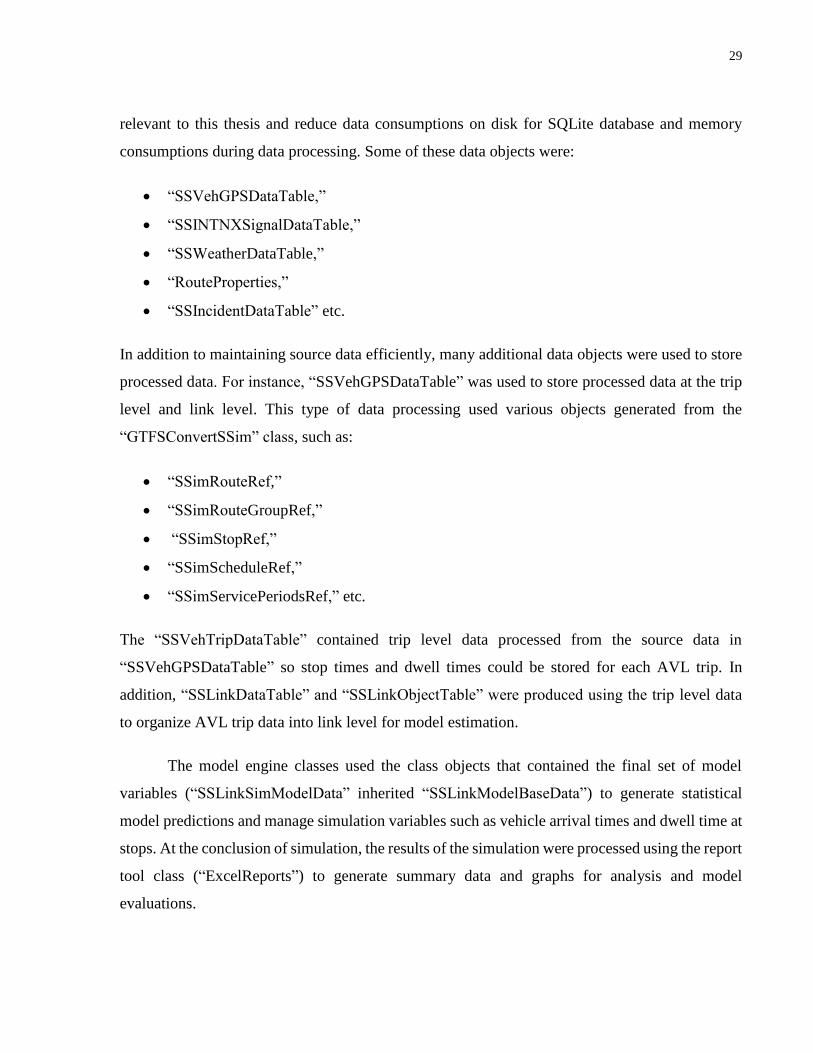
29
relevant to this thesis and reduce data consumptions on disk for SQLite database and memory
consumptions during data processing. Some of these data objects were:
• “SSVehGPSDataTable,”
• “SSINTNXSignalDataTable,”
• “SSWeatherDataTable,”
• “RouteProperties,”
• “SSIncidentDataTable” etc.
In addition to maintaining source data efficiently, many additional data objects were used to store
processed data. For instance, “SSVehGPSDataTable” was used to store processed data at the trip
level and link level. This type of data processing used various objects generated from the
“GTFSConvertSSim” class, such as:
• “SSimRouteRef,”
• “SSimRouteGroupRef,”
• “SSimStopRef,”
• “SSimScheduleRef,”
• “SSimServicePeriodsRef,” etc.
The “SSVehTripDataTable” contained trip level data processed from the source data in
“SSVehGPSDataTable” so stop times and dwell times could be stored for each AVL trip. In
addition, “SSLinkDataTable” and “SSLinkObjectTable” were produced using the trip level data
to organize AVL trip data into link level for model estimation.
The model engine classes used the class objects that contained the final set of model
variables (“SSLinkSimModelData” inherited “SSLinkModelBaseData”) to generate statistical
model predictions and manage simulation variables such as vehicle arrival times and dwell time at
stops. At the conclusion of simulation, the results of the simulation were processed using the report
tool class (“ExcelReports”) to generate summary data and graphs for analysis and model
evaluations.
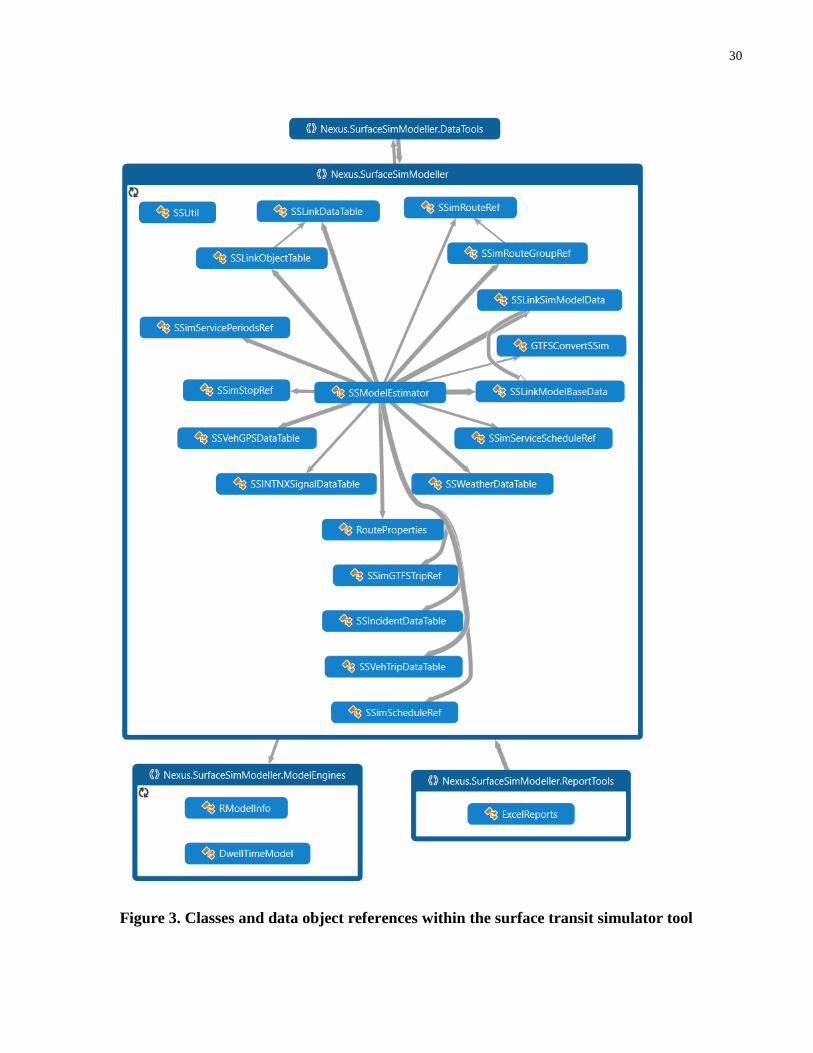
30
Figure 3. Classes and data object references within the surface transit simulator tool

31
3.3.2 Program Components
Within each of the class objects, methods were defined to carry out the required procedures
of the program. Figure 4 illustrates how the various functional components of the program interact
to carry out the required functions by making calls to each other. As mentioned previously, the
simulator program functions include data collection, data processing, model estimation, and model
simulation with variables on temporal effects, transit operational characteristics, expanded link
characteristics, route characteristics, and disruption characteristics. Modular program components
each carry out a particular procedure that enables these functions.
The first group of methods handle the data collection. The “DownloadNextBusGPSData”
method queries real-time NextBus API online to retrieve AVL data and save these data offline for
processing (see section 0 for source code). To gather weather data, the “DownloadWeatherData”
method retrieves real-time weather information from OpenWeatherMap APIs (see section A.1.3
for source code). The Toronto road restriction data were gathered via the open data Toronto road
restriction API with the “DownloadTorontoIncidentData” method (see section A.1.4 for source
code). These methods were used to gather online real-time data needed for modelling.
Once the data were downloaded, the offline data files containing all of the required data
sources were loaded into the program. The modular design of the methods means that
“LoadDataFromOfflineFile” loaded various offline data into memory and updated them in the
SQLite database by calling different methods such as (see section A.1.5 for source code):
• “LoadGTFSReferenceData” to load GTFS data from GTFS database (see section A.1.6
for source code);
• “InitializeGPSTripDb” to load AVL GPS data and process GPS trips and “Update-
AndLoadGPSDbDataFromFiles” to load and update database table;
• “UpdateDbWeatherDataFromFiles” to load weather data from file and update database
table, or “GetWeatherDataFromDB” to load weather data from database table;
• “UpdateDbIncidentDataFromFiles” to load road restriction data from file and update
database table, or “GetTorInciDataFromDB” to road restriction data from database table.

32
After the data were loaded, data processing could be done by calling “ProcessGPSData”
method (see section A.2.1 for source code). The “ProcessGPSData” method checked if the AVL
trip information contained fully process stop times, dwell times, as well as respective link data
with all the necessary attributes. The first stage of the data processing was to determine the
schedule ID of the AVL or GPS trips. This was performed by the method
“ScheduleMatchingGPSTripWithGTFS” (see section A.2.2 for source code). The determination
of schedule ID allowed the “DetermineAllFeatureValues” method to proceed in finding the
observed stop times (see section A.2.3 for source code). The GPS trips were preprocessed and
organized for arrival and dwell time computation using the method
“ProcessAndOrganizeGPSPointsForTrip” (see section A.2.4 for source code). Then, the
“EstimatedArrivalAndDwellAlongScheduleRoute” method was called to determine arrival and
dwell times for every stop along the GPS trips (see section A.2.5 for source code). By comparing
the observed arrival and dwell times to the schedule information, all of the transit operational
characteristics could be found. After the trip data were processed, these data were processed into
link data with “InitializeModelLinksToDb” method (see section A.2.6 for source code). Expanded
link characteristics, route characteristics, and disruption characteristic were obtained using
“GetIntxnIDsAndInitialDataForLinkObj” and “GetIntxnDataMissingVolAndStopLoc” methods;
these methods geotemporally match data records from different data sources to obtain additional
characteristics for a transit trip (see section A.2.7 and section A.2.8 for source code). In addition,
stop locations were obtained using the relative positions between stops and intersections; the stop
locations data were stored in a database table using the “UpdateStopDataToDB” method (see
section A.2.9 for source code). After link objects and link data were finalized, the
“UpdateAllLinksToDB” method was called to update the database with the link data information
(see section A.2.10 for source code). These link data were exported for model estimation and
simulation.
Once data processing was completed, the attributes associated with each observation on a
transit link can be used to estimate the running speed and dwell time models. The estimation of
running speed models was done in C# and R using the “RModel_RunningSpeedModelEstimation”
33
method in C# and “ME_TaskHandler” script in R (see section A.3.1 and A.3.3 for source code).
The following packages were used to estimate running speed models:
• the “MASS” package for multiple linear regression models (Ripley et al., 2017),
• the “e1071” and “liquidSVM” packages for support vector machines (Meyer et al., 2017;
Steinwart & Thomann, 2017),
• the “lme4” package for linear mixed-effects models (Bates et al., 2017, p. 4),
• the “rpart” package for regression trees (Therneau, Atkinson, & Ripley, 2017),
• the “ranger” package for fast implementation of random forest (Wright, 2017).
In addition, dwell time models were estimated in C# using the “Model_StopModelsEstimation”
method (see section A.3.2 for source code). The lognormal distribution estimator from the
Math.Net Numerics library in C# was used to estimate the parameters of the dwell time models
(Christoph Rüegg et al., 2017). After estimating running speed and dwell time models, transit trips
were initialized using a set of test data from “ImportLinkDataForModelRef” and GTFS schedule
trip data from “LoadGTFSReferenceData” (see section A.4.1 and section A.1.6 for source code).
Using the initialized trips, the “GetPredictionForLinkDataInR” method was able to generate
running speed and dwell time predictions for simulated transit trips (see section A.4.2 for source
code). Then, the “Model_GenerateReportsWithBinFileAndR” method generated detailed
summary data and graphs using the simulated transit trips results (see section A.5.1 for source
code). This method called three separate methods to generate three types of reports. The method,
“CreateTimeDistDiagramReport”, generated excel line graphs showing the vehicle trajectories of
simulated, scheduled, and observed trips (see section A.5.2 for source code). Another method,
“CreateStopDelayReport”, produced stop level reports for model validation. Similarly,
“CreateRouteSpeedReport” generated route level reports for model validation.

34
Figure 4. Functional component calls within the surface transit simulator tool

35
3.4 Summary
This chapter introduced the modelling framework for the mesoscopic surface transit
simulator. Two different use cases, basic route level analysis and advanced network level analysis,
were established to determine the appropriate functional requirements. The functional
requirements for this simulator were to represent the temporal effects, transit operational
characteristics, expanded link characteristics, route characteristics, and disruption characteristics,
by obtaining model attributes through data processing, by estimating statistical models of running
speed and dwell time, and simulating transit vehicle movements using the statistical models. A
detailed simulation framework, consisting of various components of a software pipeline, was
constructed based on these function requirements (see Figure 2). Then, the function design
components of the simulator were detailed with respect to the class object references and program
component calls. The class objects contained data fields and methods to store data and carry out
functional procedures, respectively. In addition, the methods within each of those classes carried
out the specific procedures, using fields and method calls, to fulfil the functional requirements of
the program (see Figure 3). This chapter detailed the functional design of the surface simulator
program, based on function design approach, object-oriented programming paradigm, and cross-
language interoperability. The final program design is highly modular and extensible for additional
data sets, training new types of models, and new transit networks.

36
Chapter 4
Data Collection
One of the first steps in building an automatic modelling pipeline is data collection. This
chapter details the different procedures used to collect and manage data from online open data
sources. A collection of these data enabled the program to perform the functions required by its
functional design. Data for this thesis were obtained in two ways: historical open data archives and
real-time open data feeds. Real-time open data feeds required the use of online APIs with multiple
download threads for simultaneous real-time data collection. Archival open data required data
conversion to enable automatic data processing.
This chapter discusses the use of different data collection methods for transit network data,
such as GTFS, AVL, road restriction, weather, and traffic intersection data. The choice of these
data was based on previous literatures on transit travel time regression models. In addition to transit
operational parameters such as headway and delay, previous studies have used disruptions,
weather conditions, time of day, and day of the week to model the various effects on transit travel
times (X. Chen et al., 2004; Yu et al., 2006). In this thesis, road restriction data were collected to
examine the effect of roadway closure disruptions have on transit travel times. Weather data were
also collected to examine the effect of weather parameters such as precipitation. Finally, the
specific time of day and day of the week of the transit travel were used to examine temporal effects.
In addition to the variables used by the previous studies, this thesis also accounts for the effect of
transit stop locations using the traffic intersection data for Toronto.
4.1 Data Collection Methods
This section presents the processes used to collect historical open data archives and real-
time open data feeds. An established method to collect open data ensured consistent data structure,

37
data quality, and data storage format. The consistent data structure for particular data sets or even
groups of similar data sets allowed different data sets to be fused and create more informative
attributes for analysis. A standardized method of collecting data, especially when done
automatically, maintained a consistent data format for analysis. Finally, a predetermined data
storage format ensured readability of the data. This thesis used common open standard file and
database formats, such as Extensible Markup Language (XML) and JavaScript Object Notation
(JSON), to store the collected data.
4.1.1 Historical Open Data Archives
Historical open data archives that were stored in formats such as comma-separated value
(CSV) formats or text formats were converted into formats such as XML and JSON. XML and
JSON are human-readable because they are text-based with words and numbers that can be viewed
easily without the need for conversion. These formats are machine-readable because the words and
numbers containing data are qualified with the name and type of fields. The properties of XML
and JSON file format make them suitable candidates to deliver and store historical open data.
The flowchart below outlines the steps to convert historical open data archives into XML
or JSON file formats. The historical data was first downloaded manually. Then, these data were
unpackaged, manually validated, and saved as text-based CSV files. The prepared data were
converted to XML or JSON objects with a short script that read the text file and properly formats
the data types of each field. Finally, the converted XML or JSON objects were saved. The schema
of these XML or JSON objects could be used to read these files into program memory.
Figure 5. Data collection for archival data
Manually Download
Archival Data
Unpack archive and validate
data
Convert archive to XML or JSON
Object
Save XML or JSON File

38
4.1.2 Real-time Open Data Feeds
Traditionally, open data were usually archives and records published by organizations
periodically. Recent efforts in the digitalization of real-time data records by governments and
organizations made available many real-time data streams such as the automatic vehicle locations,
weather conditions, and road restrictions. Unlike archival data, real-time data streams require
continuous polling and downloads from APIs, as well as management of the downloaded data.
Using programming code developed for this thesis, the real-time online API data were downloaded
(see section A.1 for source code).
The first step in downloading real-time data was to initiate download session, as shown in
Figure 6. In this step, the “end of the download” time is assigned and checked against the current
time. If the current time is before the “end of the download” time, then the next download request
is scheduled based on the polling rate. For instance, if the polling rate of the download is 20
seconds, then the next download request is to take place 20s after the previous download request.
Then, the program will wait until the download request execution time to send an asynchronous
web client download request to the web API server. After a brief wait, the web server returned an
API response object. This API response object was converted into desired data structure and
checked for duplicates. The converted data was then saved into memory or disk. The download
cycle continued until the “end of the download” time was reached. At the end of the download, all
the data were saved to disk.

39
Figure 6. Data collection for real-time online API data
4.2 Open Data Formats and Collections
There were five open data sources used by this thesis. The classes and data objects used to
read and convert these data are presented in Figure 7. In the following sections, methods used for
data collection are outlined. Then, the format of the downloaded data is presented. Finally, the data
conversion process to prepare the data for data processing are discussed. The type of information
each open data source contains determined the attributes that could be obtained for modelling.
Initiate Download
•Check current time
•If greater than end of download time, save and terminate.
•If less, schedule next download request.
Sends Asynchronous WebClient Download Request
•Wait for response
•Get Web API response object
Data Conversion
•Convert to defined structure
•Eliminate duplicates
Save
•If reached schedule save, add to memory object and save to disk.
•Otherwise, save to memory object.
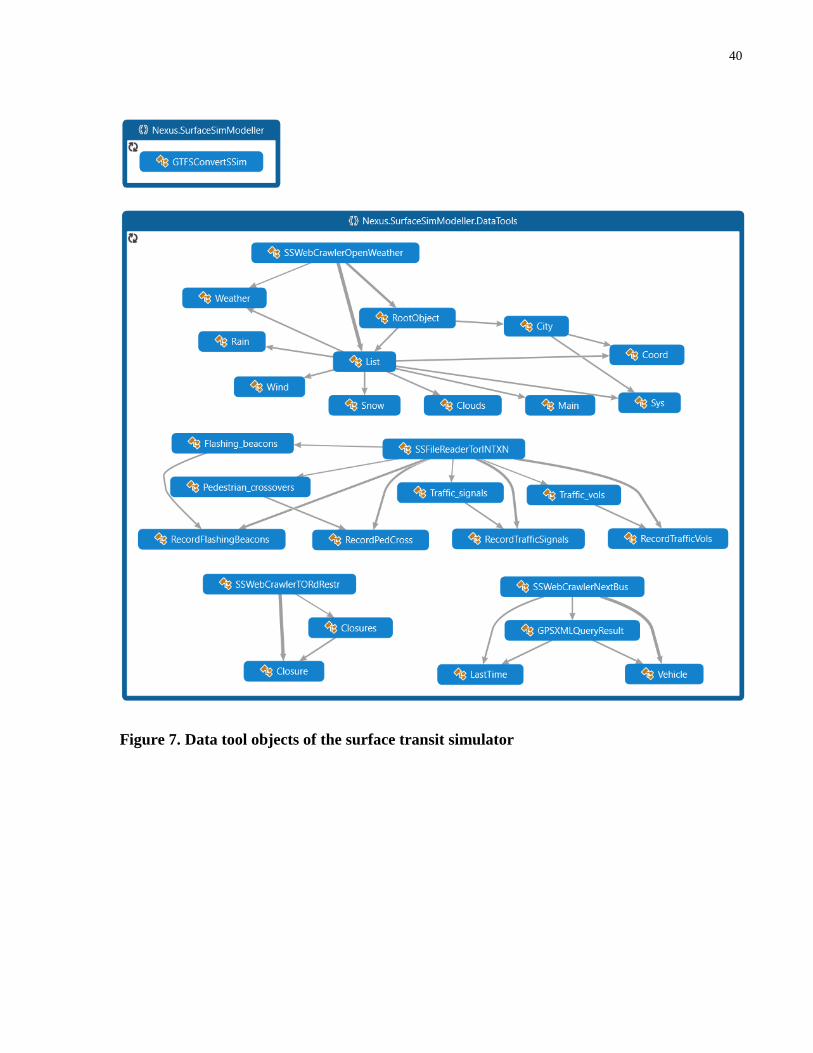
40
Figure 7. Data tool objects of the surface transit simulator

41
4.2.1 General Transit Feed Specification
General Transit Feed Specification (GTFS) data for the Toronto transit network contained
the schedule information of all transit trips in the network. The GTFS data were manually
downloaded from TransitFeeds (TransitFeeds, 2016). The format of the GTFS schedule data was
CSV. The CSV files contained data about the transit agency, service periods, routes, shapes of
routes, stop times, stops, and trips. The fields of each of the CSV files are outlined in the following
table. The data were then organized into vehicle trips using a GTFS converter,
“GTFSConvertSSim”. The details regarding how the GTFS converter process the original CSV
files can be found in section 5.1.1. The GTFS data contained detailed information regarding transit
services at the network level; these data were used extensively during all stages of the simulation
such as data processing, model estimation, and model simulation, where the schedule data were
required.
Table 1. Fields for GTFS CSV files
CSV File Name of Field Description of Field
Agency.CSV agency_id the id number of agency
agency_name the name of the agency
agency_url the web address of the agency
Calendar.CSV service_id the id of the service period
Monday, Tuesday,
Wednesday, Thursday,
Friday, Saturday, Sunday
a list of the days this service period includes
start_date the start date of the service period
end_date the end date of the service period
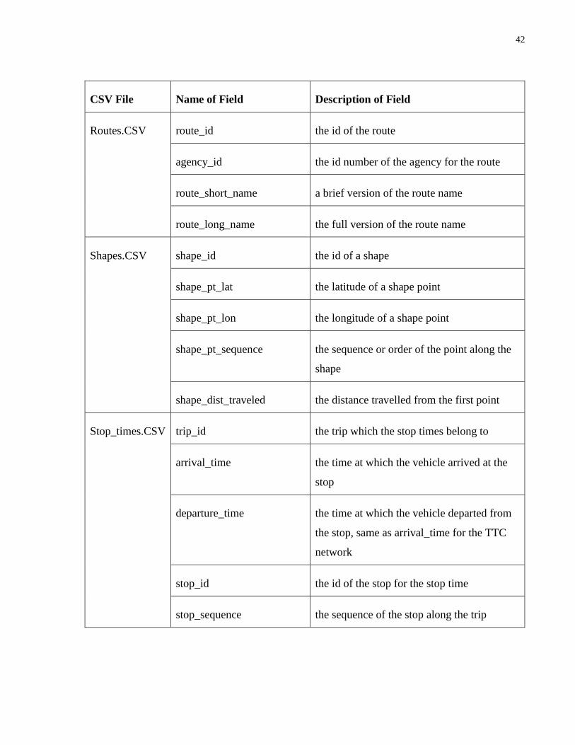
42
CSV File Name of Field Description of Field
Routes.CSV route_id the id of the route
agency_id the id number of the agency for the route
route_short_name a brief version of the route name
route_long_name the full version of the route name
Shapes.CSV shape_id the id of a shape
shape_pt_lat the latitude of a shape point
shape_pt_lon the longitude of a shape point
shape_pt_sequence the sequence or order of the point along the
shape
shape_dist_traveled the distance travelled from the first point
Stop_times.CSV trip_id the trip which the stop times belong to
arrival_time the time at which the vehicle arrived at the
stop
departure_time the time at which the vehicle departed from
the stop, same as arrival_time for the TTC
network
stop_id the id of the stop for the stop time
stop_sequence the sequence of the stop along the trip
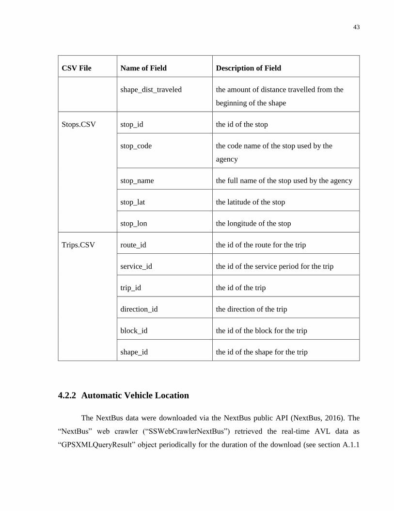
43
CSV File Name of Field Description of Field
shape_dist_traveled the amount of distance travelled from the
beginning of the shape
Stops.CSV stop_id the id of the stop
stop_code the code name of the stop used by the
agency
stop_name the full name of the stop used by the agency
stop_lat the latitude of the stop
stop_lon the longitude of the stop
Trips.CSV route_id the id of the route for the trip
service_id the id of the service period for the trip
trip_id the id of the trip
direction_id the direction of the trip
block_id the id of the block for the trip
shape_id the id of the shape for the trip
4.2.2 Automatic Vehicle Location
The NextBus data were downloaded via the NextBus public API (NextBus, 2016). The
“NextBus” web crawler (“SSWebCrawlerNextBus”) retrieved the real-time AVL data as
“GPSXMLQueryResult” object periodically for the duration of the download (see section A.1.1

44
for source code). For every download, the “LastTime” object attached to each query batch was
used to determine the exact time of the observation of the vehicle location in an array of the
“Vehicle” object. The vehicle objects contained several fields detailed in the following table. The
observed “Vehicle” fields were converted to “SSVehGPSDataTable” with assigned gpsID,
GPStime, vehID, longitude, latitude, direction, heading, and tripCode (that contained route
number, branch number and vehicle id). The converted AVL data was used during data processing
to retrieve attributes such as arrival and dwell times.
Table 2. Vehicle object fields for NextBus AVL XML files
Field Name Field Description Example data
id the id of the vehicle 4187
routeTag route number of the vehicle 512
dirTag route number, direction, and
branch number of the vehicle
concatenated with an
underscore
512_1_512
lat latitude of the observed
vehicle
43.673367
lon longitude of the observed
vehicle
-79.463783
secsSinceReport the number of seconds since
the last report
10
heading the heading of the vehicle 253
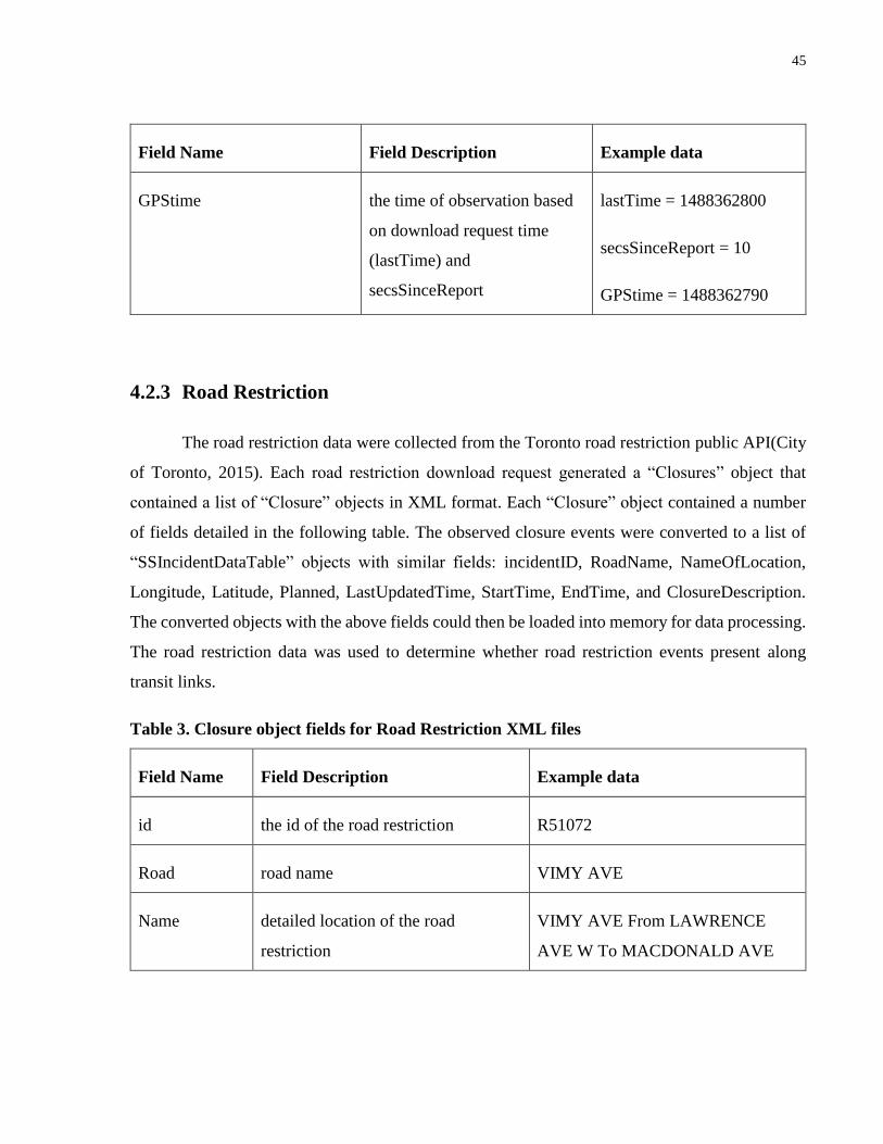
45
Field Name Field Description Example data
GPStime the time of observation based
on download request time
(lastTime) and
secsSinceReport
lastTime = 1488362800
secsSinceReport = 10
GPStime = 1488362790
4.2.3 Road Restriction
The road restriction data were collected from the Toronto road restriction public API(City
of Toronto, 2015). Each road restriction download request generated a “Closures” object that
contained a list of “Closure” objects in XML format. Each “Closure” object contained a number
of fields detailed in the following table. The observed closure events were converted to a list of
“SSIncidentDataTable” objects with similar fields: incidentID, RoadName, NameOfLocation,
Longitude, Latitude, Planned, LastUpdatedTime, StartTime, EndTime, and ClosureDescription.
The converted objects with the above fields could then be loaded into memory for data processing.
The road restriction data was used to determine whether road restriction events present along
transit links.
Table 3. Closure object fields for Road Restriction XML files
Field Name Field Description Example data
id the id of the road restriction R51072
Road road name VIMY AVE
Name detailed location of the road
restriction
VIMY AVE From LAWRENCE
AVE W To MACDONALD AVE

46
Field Name Field Description Example data
District the name of the city district Etobicoke York
Latitude the latitude location 43.702751
Longitude the longitude location -79.504901
RoadClass Major Arterial the type of road
Planned an indication of whether the event is
planned or unplanned
1 – yes
LastUpdated the time last updated 1486701720000
StartTime the start time of the restriction 1487062800000
EndTime the end time of the restriction 1487174400000
Description description of the nature of road
restriction
The northbound and southbound
lanes will be alternately occupied
due to construction.
4.2.4 Weather
The weather data were downloaded from the OpenWeatherMap public API
(OpenWeatherMap, 2017). Unlike other open data formats, the download weather data was highly
hierarchical and very complex with many data objects (see “SSWebCrawlerOpenWeather” in
Figure 7). The “RootObject” object returned from weather API query contain several objects with
multiple fields, as detailed in the following data. The information contained in the weather objects
were converted to “SSWeatherDataTable” object with reduced data complexity and similar fields
such as:
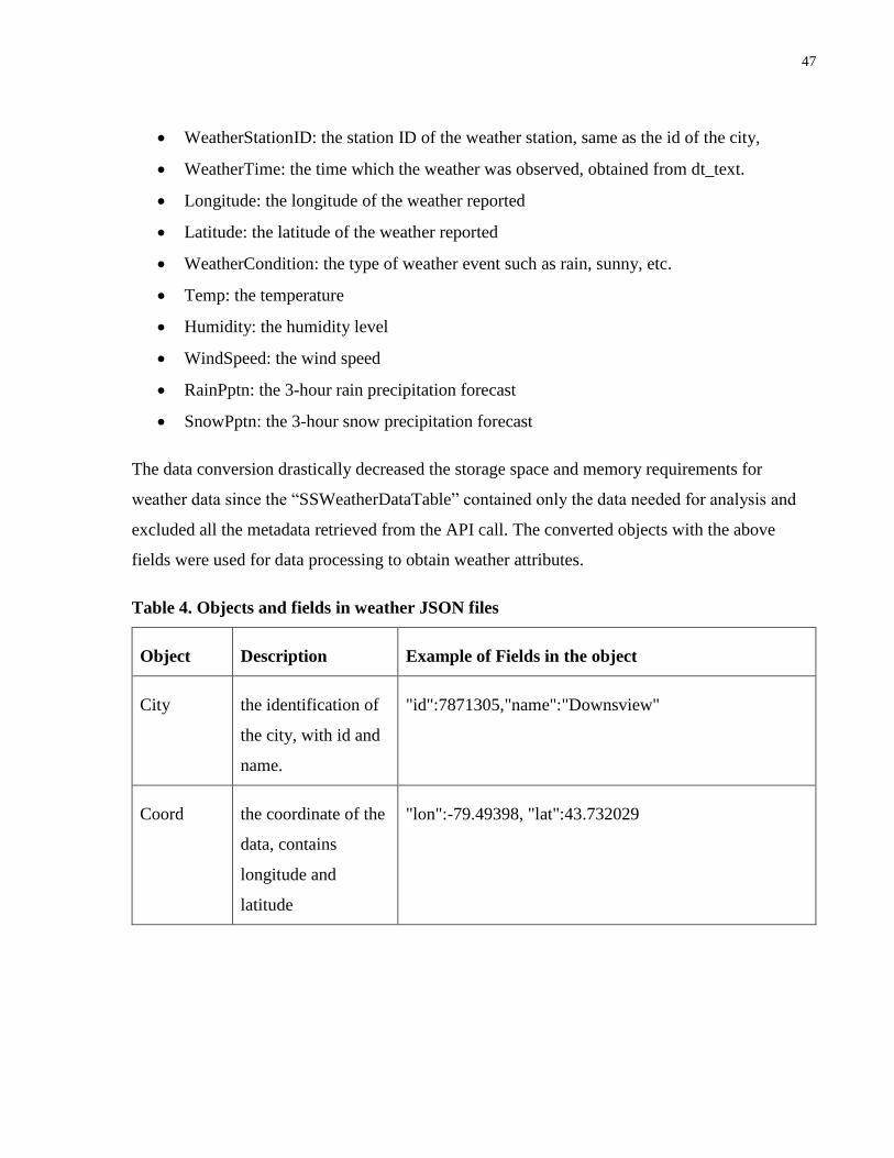
47
• WeatherStationID: the station ID of the weather station, same as the id of the city,
• WeatherTime: the time which the weather was observed, obtained from dt_text.
• Longitude: the longitude of the weather reported
• Latitude: the latitude of the weather reported
• WeatherCondition: the type of weather event such as rain, sunny, etc.
• Temp: the temperature
• Humidity: the humidity level
• WindSpeed: the wind speed
• RainPptn: the 3-hour rain precipitation forecast
• SnowPptn: the 3-hour snow precipitation forecast
The data conversion drastically decreased the storage space and memory requirements for
weather data since the “SSWeatherDataTable” contained only the data needed for analysis and
excluded all the metadata retrieved from the API call. The converted objects with the above
fields were used for data processing to obtain weather attributes.
Table 4. Objects and fields in weather JSON files
Object Description Example of Fields in the object
City the identification of
the city, with id and
name.
"id":7871305,"name":"Downsview"
Coord the coordinate of the
data, contains
longitude and
latitude
"lon":-79.49398, "lat":43.732029

48
Object Description Example of Fields in the object
Main the typical weather
information
including,
temperature range,
pressure, sea level,
ground level,
humidity.
"temp":270.59, "temp_min":270.59, "temp_max":270.9,
"pressure":992.76, "sea_level":1027.49,
"grnd_level":992.76, "humidity":68
List an object that holds
detailed weather data
see the following rows
Clouds the type of clouds "clouds":null
Snow the expected 3-hour
snow precipitation
"snow":{"3h":0.065}
Rain the expected 3-hour
rain precipitation
"rain":{"3h":0.0}
Weather contains weather
display objects
properties
"weather":[{"id":600,"main":"Snow","description":"light
snow","icon":"13n"}]
Sys general and other
information about
the data point
"sys":{"country":null,"population":0,"pod":"n"}
49
4.2.5 Traffic Intersection Characteristics
The traffic intersection and signal data files were downloaded manually from Open Data
Toronto (City of Toronto, 2017c, 2017b). There were four data files for traffic intersection
characteristics: “flashing_beacons.XML”, “pedestrian_crossovers.XML”, “traffic_signals.XML”,
“traffic_vols.XML”. Each of the data files had corresponding XML objects (one object as
individual records, one object as the container of an array of records) as shown in Figure 7. The
first three data files contained detailed data about the intersections, such as intersection ID, street
names and geographical locations (longitude and latitude) of the flashing beacon device, pedestrian
crossover signals, and traffic light signals. These data were helpful in determining the locations
where transit vehicles may have encountered potential delays due to flashing beacon warnings,
pedestrians crossing mid-block sections of the street, or signals delays at intersections. The fourth
data file contained the traffic volume count data at most of the signalized intersections. The volume
data included the count date, 8-hour vehicle count and 8-hour pedestrian count in addition to
identifying information about the intersection. The volume data could be used to determine general
traffic levels at each intersection.
Although there were four different data files for traffic intersections, a common data type
was defined for loading all of the data files since almost all of the fields exist in each of the files.
As such, the four data files were converted to “SSINTNXSignalDataTable” data type for data
processing. The “SSINTNXSignalDataTable” data type contained all of the fields present in any
of the four intersection data files: intersectionID (“pxID”), mainStreetName,
midBlockStreetName, sideStreetNames, Latitude, Longitude, countDate, vehVol, pedVol,
signal_system, mode_of_control, and type_Of_Intersection (signalized intersection, pedestrian
crossing, or flashing beacon). A common data type for all the four data files allowed the traffic
volume data to be merged with intersection properties where the pxID were identical. After data
conversion, the intersection data could be used during data processing to obtain intersection related
attributes between transit stops.

50
4.3 Summary
This chapter detailed the method used to perform data collection. This thesis used manual
download and data conversions to collect historical open data archives and used automatic multi-
threaded online API web requests to collect real-time open data feeds. The five major data sets
used in this study were GTFS, AVL, road restriction, weather, and traffic intersection data. The
format of the original data source was presented. The original data were converted to a new format
for lower data size, reduced data complexity, and common data type. The converted data types
could be loaded into memory and saved into SQLite database tables for data processing.

51
Chapter 5
Data Processing
While big data from open data sources provide researchers with vastly more information
to analyse and study, the value of open data may not be fully realized without a systematic and
computationally efficient method of data processing. Many of the open data formats were
unstructured, so they were not suitable for modelling and analysis. To retrieve valuable
information from these data, they must be processed. Unstructured data are data with a low degree
of organization. Processing unstructured data into structured data with target labels and defined
attributes and variables enables the estimation of models. For example, the AVL source data was
composed of a large list of GPS points with information such as longitude, latitude, route number,
vehicle number, and direction of travel (S/N or E/W). These data labels could be used to process
the AVL data into vehicle trips with variables of interests such as trip id, stop times, running
speeds, dwell times, and delays. After such processing, the structured AVL data could be analysed
and be used for modelling. To process these data efficiently, a cross-platform relational database
management system called SQLite was used to manage application data.
There were four stages involved in an automatic data processing procedure used for this
thesis: data loading, preprocessing, processing, and data export. The detailed processing
procedures for each data set following the four main stages are discussed in the following sections.
Figure 8. Data Processing Flow
Data LoadingPreprocessing or Preparation
Processing
•Trip Processing
•Map Matching
Data Export
52
5.1 Data Loading
Data loading refers to the process of copying source data from files or databases onto
memory objects used by the processing procedure. This section describes the formats of the
collected data files, and the process used to load them into memory. As open data formats evolve,
the data loading processes used can differ, but the general idea of loading these data to enable data
processing should remain the same. The following sections detail the data loading process of
GTFS, AVL, road restriction, weather, traffic intersection, and transit route property data.
5.1.1 General Transit Feed Specification
While comma separated value (CSV) format are commonly used, the GTFS CSV files are
quite difficult to use at runtime when retrieving attributes related to transit trips. This is due to the
unstructured nature of these CSV files. There were eight CSV files for the Toronto Transit
Commission (TTC) network: agency.CSV, calendar.CSV, calendar_dates.CSV, routes.CSV,
shapes.CSV, stop_times.CSV, stops.CSV, and trips.CSV. Each of these files contained all the
information regarding the file name of the CSV. For instance, stops.CSV contained the stop id,
stop code, stop description as well as the longitude, the latitude of all the transit stops in the
network. The user of this data was expected to use this data and refer to other CSVs with additional
data about the stops. The stop_times.CSV contained all the scheduled times that the transit vehicles
made a stop, for a trip at a stop. Given the trip id of those stop times, the stop times with stop
locations could then be traced to a trip in the trips.CSV file. Then, the trips.CSV contained further
information about the trip such as route id, which established the characteristics of the routes in
routes.CSV. The routes data had information about the agency, as well as the calendar dates which
the route serviced. The original GTFS CSV files minimized the storage requirements of these files
but made their use at runtime more difficult.
To use the GTFS CSV files efficiently at run time, they were processed into a network of
vehicle trips with their corresponding stop times and travel paths. For this thesis, a GTFS converter
was used to transform these CSV files into an SQLite database file with various tables on vehicle
trips, routes, and stops. This GTFS converter had been originally used by the Nexus Platform for
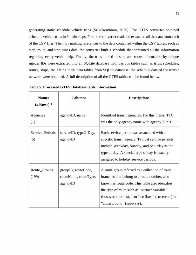
53
generating static schedule vehicle trips (Srikukenthiran, 2015). The GTFS converter obtained
schedule vehicle trips in 3 main steps. First, the converter read and extracted all the data from each
of the CSV files. Then, by making references to the data contained within the CSV tables, such as
stop, route, and stop times data, the converter built a schedule that contained all the information
regarding every vehicle trip. Finally, the trips linked to stop and route information by unique
integer IDs were extracted into an SQLite database with various tables such as trips, schedules,
routes, stops, etc. Using these data tables from SQLite database, the schedule data of the transit
network were obtained. A full description of all the GTFS tables can be found below.
Table 5. Processed GTFS Database table information
Names
(# Rows) *
Columns Descriptions
Agencies
(1)
agencyID, name Identified transit agencies. For this thesis, TTC
was the only agency name with agencyID = 1.
Service_Periods
(5)
serviceID, typeOfDay,
agencyID
Each service period was associated with a
specific transit agency. Typical service periods
include Weekday, Sunday, and Saturday as the
type of day. A special type of day is usually
assigned to holiday service periods.
Route_Groups
(199)
groupID, routeCode,
routeName, routeType,
agencyID
A route group referred to a collection of route
branches that belong to a route number, also
known as route code. This table also identifies
the type of route such as “surface variable”
(buses or shuttles), “surface fixed” (streetcars) or
“underground” (subways).

54
Names
(# Rows) *
Columns Descriptions
Routes
(3,405)
routeID, groupID, name This table described the route branches in a route
group, and linked the route branches to the main
route number.
Stops
(10,570)
stopID, stopCode,
Longitude, Latitude,
stopType, stopName
The location of stops was defined by longitude
and latitude, while the stops were identified by
stop ID, stop code and stop name.
Schedule
(3,405)
scheduleID, serviceID,
routeID, groupID,
routeStops,
routeStopDistances,
shapeID
The schedule table contained the list of stops and
stop shape distances, as well as the path (shape)
which the transit vehicle travelled. The list of
stops IDs, distances and path for a schedule was
stored in the sequencing service. Each schedule
corresponded to each route with a route name, as
well as a service period with a type of day.
Shapes
(1,515)
shapeID, path Each path in the Shapes table contained a
sequence of high-resolution geographical
locations, defined by longitude and latitude.
Trips
(133,361)
tripID, scheduleID,
blockID, shapeID,
stopTimes
The trip table contained all the scheduled transit
trips over each day of service. The sequence of
stop times in each trip corresponded to a
sequence of stops and stop distances in the
schedule table with the corresponding
scheduleID.
* based on TTC GTFS schedule data between February 12, 2017 and March 25, 2017.
55
There were many benefits of converting the original CSV files to database tables during
the data loading step. Firstly, the process of converting the CSV files into linked trip objects with
detailed properties such as stop ID, stop distances, stop times, and paths took a considerable
amount of time – approximately five minutes, while the reading of the processed GTFS data takes
much less time. By processing the GTFS schedule during or before data loading, we reduced the
time associated with loading the routed transit trips from five minutes down to 30 seconds, for
each data processing run. Also, this eliminated the need to process GTFS data at run time, as
processed GTFS data could be simply saved to disk and be loaded quickly when they were needed
at the beginning of data processing. In addition, loading fully processed scheduled data allowed
for faster referencing during AVL data processing. Finally, this was beneficial to parts of the thesis
beyond data processing, such as model estimation and model simulation, as those algorithms relied
heavily on the ability to reference GTFS schedule as well for key information.
5.1.2 Automatic Vehicle Location (AVL)
Since the AVL data collected were stored in XML files divided up by each hour, the data
loading of AVL data consisted of two steps: loading XML files into memory and combining all
data objects. The file names of AVL XML data files used were in the format of “all-GPS-
yyyymmddhhmmss-yyyymmddhhmmss.XML.” The first and second date time string consisted of
the start and end year, month, day, hour, minute, and second, respectively. The date time string
used the UTC time to prevent duplicate names due to daylight saving time. Using this naming
convention, the XML file names falling within the study period were loaded into memory as a
dictionary of “SSVehGPSDataTable” indexed by GPS ID. After the XML files were loaded, each
AVL point was checked for uniqueness by the time of observation and vehicle ID. Duplicated data
were ignored during AVL data loading. After AVL data points were loaded into memory, they
were inserted into the “TTCGPS” table in the Surface Simulator (SSim) database. The SSim
database was a separate database from the GTFS database generated earlier and it was used to store
and process real-time transit related data. The data points from AVL data were used extensively
to compute various operational characteristics of the observed transit trips.
56
5.1.3 Road Restriction
The road restriction data also used XML format for storage, but due to the smaller sizes of
the data, this data was stored by day with a similar naming convention: “all-RR-
yyyymmddhhmmss-yyyymmddhhmmss.XML”. Using such a naming convention, all the required
road restriction data were loaded into the program as a dictionary of “SSIncidentDataTable”
indexed by incident ID and were ready to be used for processing. After loading these data into
memory, they were inserted into the “TORINC” table in the SSim Database. The road restriction
data were used to determine the presence of potential incidents due to emergency and road work,
which resulted in reduced road capacities and potential travel delays.
5.1.4 Weather
Similar to road restriction data, weather data had smaller sizes as well, as such, the weather
JSON files were stored by day with a naming convention such as: “GTA-Weather-
yyyymmddhhmmss- yyyymmddhhmmss.json”. All the required weather data were loaded into
memory as a dictionary of “SSWeatherDataTable”, indexed by weather record ID for data
processing. The weather data had detailed temperature and precipitation across many weather
station for a defined geographical area such as the Greater Toronto Area (GTA).
5.1.5 Traffic Intersection Characteristics
Unlike AVL, road restriction, and weather data, traffic intersection data were archived data.
For easier data loading, the various traffic intersection data originally in CSV format were
converted into XML format. These traffic data files, namely “flashing_beacons.XML”,
“pedestrian_crossovers.XML”, “traffic_signals.XML”, and “traffic_vols.XML”, were loaded into
memory with a common object type named “SSINTNXSignalDataTable”, indexed by intersection
(px) ID. The intersection data were used to determine the intersection-related attributes for transit
network.

57
5.1.6 Transit Route Properties
While GTFS contains route identifications, additional properties of the transit route may
be needed to introduce more descriptive characteristics to transit routes. For this thesis, a custom
route properties data object, stored in XML format, was created to identify whether each route
number in the Toronto Transit Commission is a streetcar and has dedicated right of way (ROW).
The route properties data were loaded during data loading step as a list of “RouteProperties”. These
data were used for determining route attributes during data processing.
5.2 Preprocessing of AVL data
Due to equipment and communication errors, a small fraction of the real-time AVL data
did not contain meaningful information for analysis. AVL data preprocessing addressed three main
data issues: empty data, non-revenue trip data, and wrongly labelled data. These erroneous data
points could cause problems in many steps of data processing, including the proper forming of
trips and computations of attributes. Due to these potential issues related to erroneous AVL data
points, the AVL data needed to be preprocessed.
5.2.1 Empty Data
Most modern AVL systems rely on Global Positioning Systems (GPS) to triangulate the
positions of transit vehicles and report them in real-time via cellular service or radio
communications. Often, during initialization of the GPS system, a default geographical location
stored by the GPS device is reported. This default location for the Toronto Transit Commission
AVL system was (latitude = 43.5 and longitude = -79), which is in the middle of Lake Ontario.
Often, a series of these default location data were received at the beginning of a vehicle’s operation
while its AVL system is trying to establish GPS triangulation. Data points with this default location
were considered empty data and were removed from the AVL data records during the data
preprocessing step.
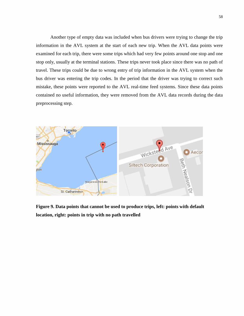
58
Another type of empty data was included when bus drivers were trying to change the trip
information in the AVL system at the start of each new trip. When the AVL data points were
examined for each trip, there were some trips which had very few points around one stop and one
stop only, usually at the terminal stations. These trips never took place since there was no path of
travel. These trips could be due to wrong entry of trip information in the AVL system when the
bus driver was entering the trip codes. In the period that the driver was trying to correct such
mistake, these points were reported to the AVL real-time feed systems. Since these data points
contained no useful information, they were removed from the AVL data records during the data
preprocessing step.
Figure 9. Data points that cannot be used to produce trips, left: points with default
location, right: points in trip with no path travelled

59
5.2.2 Non-Revenue Trip Data
Occasionally, drivers entered the trip code and left the AVL system on when they were
performing non-revenue trip from the garage to their first stop of service. This was evident
because, for some trips, the AVL points were off route at the beginning and/or at the end of the
trip where the bus garages were located. It was important to exclude these non-revenue trips
because points off route may lead to misidentifications of stop times during data processing. To
remove these points, the proximities of the AVL point from the schedule route stops were
determined. Once the points that were off the route and far away from route stops were found, they
were identified as the non-revenue trip with no stops made on their route to the garage. These non-
revenue points were then removed from the rest of the trip.
Figure 10. Non-revenue trip for AVL points labelled as King Street shuttle bus

60
5.2.3 Incorrectly labelled Trips
In the original real-time AVL data, there were trips with identical trip codes but traversed
for several cycles within the same trip before they were returned to the garage. For instance, in the
figure below, the trips were all labelled westbound but half of them were travelling eastbound.
Ideally, the bus information should have been set to out-of-service when they were performing the
non-revenue trips in the eastbound direction after the transit agency serviced customers from the
St Clair station to St Clair West station. Due to the temporary nature of these trips, the heading of
the trip was not changed for the duration of the shuttle service, where the buses were traversing
back and forth between the two stations.
For these type of incorrectly labelled trips, the chain of trips formed based on the
mislabelled trip codes resulted in a very long trip being formed, with points traversing back and
forth between two stations. To properly compute stop times, delays and headways, this type of
chained trips needed to be split into individual trips. In addition, the non-revenue portions of the
trip were removed. These trips were labelled travelling westbound when they were, in fact,
travelling eastbound. Based on careful observation and analysis of these incorrectly labelled trips,
they were corrected so data processing on mislabelled temporary services could be completed.
Figure 11. Multiple eastbound and westbound trips (over 10) on St Clair had the same trip
information, labelled as St Clair shuttle bus
61
5.3 AVL Trip Data Processing
Once data preprocessing was completed, the AVL data were processed to extract the
various attributes required for model estimation. Firstly, the AVL trips were formed based on their
route number, vehicle identification, and direction of travel. Then, using the newly formed trips
with their route number (route code), the branch with the closest geographical match to the trip
trajectory was found and assigned to the trip. Once the specific branch the trip belongs to was
determined, various attributes such as stop times, delay, and headways at each of the stops were
computed. Finally, the trips data were converted into link data to allow the addition of attributes
related to weather, road restriction, intersections, and stop locations for each link. These AVL data
processing steps converted the unstructured data of bus locations into a set of structured data
variables with descriptive feature representations.
5.3.1 Forming AVL Trips
When AVL data were collected, the data received contained various properties such as
route code (i.e.: 32), route tag (i.e.: 32A), vehicle ID (i.e.: 1504), and direction (i.e.: 1 for
North/West and 0 for South/East). These properties were used to determine the sequence of AVL
data points that formed the AVL trips. The route code, route tag, and vehicle ID properties of each
data point were used to identify the specific vehicle on a route. To perform more efficient queries
in the database, these three properties were combined into a string (text) called trip code. For
example, a data point with route code of “504”, route tag of “504BUS” and vehicle ID of “7609”
had a trip code of “504_504BUS_7609”. Utilizing this trip code for every AVL data point, a select
query was performed on the “TTCGPS” table in the SSim Database. The SQL query was
conducted for each route number using query statement such as “select * from TTCGPS where
routeCode=504 order by tripCode ASC”. Then, by reading these points one by one, in order, and
forming a trip where the change in trip code and/or vehicle direction occurred, a collection of
unique transit trips can be observed from the AVL data points. In the example provided in the
following figure, the query statement for route code 504, King Street, returned a total of 20879

62
rows of AVL data points for the sample data from February 28, 2017. A sample of these data is
shown and the forming of two trips with trip ID 8873 and 9843 is demonstrated.
Figure 12. Trip forming using SQL database query, top: TTCGPS table containing AVL
GPS points, bottom: TTCGPSTRIPS table containing AVL trips
TT
CG
PS
Tab
le
TT
CG
PS
TR
IP T
able
63
5.3.2 Stop Sequences
The newly formed AVL trips were much more informative than scattered individual AVL
points, but stop level attributes were still missing. A sequence of stops the trips serviced needed to
be determined. After AVL trips were formed, these unique trips had a sequence of AVL or GPS
point IDs that were used to retrieve detailed information regarding each point. Using these GPS
point IDs and their corresponding data, the branch that the trip belongs to was determined. After
the branch of the trip had been determined, the sequence of stops the trip serviced was then be
found.
5.3.2.1 Trip Route Branch Matching
For the Toronto Transit Commission (TTC) system, each route number had many branch
routes with different stop sequences. This allows the transit agency to serve the same corridor with
varying level of frequency across the line with only one route number. Some section of routes with
higher passenger demand receive more frequent service routes while other sections, usually further
away from the central business district, receive less frequent services. For example, route number
504 of King Street had two branch numbers: 504 (between Broadview Station and Dundas West
Station) and 504B (between Broadview and Queen to Roncesvalles and Queen). Many the trips’
branch routes could be found by matching the route tag from the AVL point data and the route
name in the GTFS schedule data. For clarity, these individual bus branches were equivalent to
routes in the GTFS database tables.
Unfortunately, not all the AVL trips had serviced the exact stop sequences that the GTFS
schedule suggested. Even from the sample data shown in the previous section, it was evident that
shuttle buses and temporary services were often needed to address operational challenges the
transit agency encounter daily. In fact, according to TTC’s CEO reports, in the month of May,
there were 2,603 short turned bus trips and 1,151 short turned streetcar trips(Toronto Transit
Commission, 2017a). These trips, along with the shuttle bus trips that were observed in the AVL
data, made it necessary to determine the branch the observed AVL trip was serving, especially if
the trip was a short turned or temporary trip.

64
The procedure to determine the best schedule match involved three main steps. Firstly, a
possible list of all the GTFS schedule (as each schedule ID for GTFS database has a unique route
ID for branches such as 504, 504A, with a specific time of day code such as 3 for weekday) from
the GTFS route group (i.e.: route number or route code such as 504) with the correct time of day
of service was chosen. This step reduces the number of comparisons between the GTFS route stop
sequences and the GPS points in the AVL trip. Then, a score based on the proximity of GPS points
in the AVL trip to the path of the GTFS schedule was used to determine the trip’s branch/route
matching. This match error score was the sum of all the GPS points’ distances from the path of the
GTFS schedule, the distance between the first GPS point and GTFS start stop, and the distance
between the last GPS point and the GTFS end stop. Finally, using the match score computed for
each potential GTFS schedule, the GTFS schedules were ranked and the one with the lowest match
error score was chosen to be the match.
Equation 1. Match error score for AVL trip schedule matching
Match Error Score = ∆𝒅𝒔𝒕𝒂𝒓𝒕 + ∆𝒅𝒆𝒏𝒅 + ∑ 𝒅𝒊
𝒌−𝟏
𝒊=𝟐
∆𝑑𝑠𝑡𝑎𝑟𝑡: distance from the first GPS point to closest GTFS start stop
∆𝑑𝑒𝑛𝑑: distance from the last GPS point to closest GTFS end stop
𝑑𝑖: distance from a GPS point to nearest point on the GTFS shape
5.3.2.2 Stop Sequence Trimming
In an ideal situation, the GPS points from an AVL trip were identically matched to the
locations of the stops from GTFS schedule. In this case, the stop sequence from the matched GTFS
schedule table could be used for the AVL trip without modifications. However, this was evidently
not the case due to the presence of short turn and temporary shuttle trips. To properly determine
the stop sequence for these trips, a custom stop sequence for the AVL trip was determined.
The stop trimming algorithm worked by first finding the closest stop to the first and last
GPS points. The result of this search could be obtained by finding the distances from the GPS

65
point to all the stops in the chosen GTFS schedule. Once the stop indices of the likely first and last
stops were determined, based on minimum distances, the algorithm deleted the stops that the AVL
trip never visited, from the stop sequence list for the AVL trip. This algorithm is illustrated in the
following figure.
Figure 13. Stop sequence trimming to delete stops not traversed by the observed trip
The stop sequence trimming step in the AVL trip data processing procedure enabled the
analysis of short-turn trips and shuttle bus trips, which did not adhere to scheduled trips’ standard
stop sequences. After stop sequence trimming, the AVL trip was ready for further processing and
attribute extraction. To make the following data processing tasks more efficient, the GPS points in
the AVL were placed in a list inside a dictionary with stop ID as the key. Each of the list placed
within the dictionary with a key was assembled in order of their distance from the start of the trip.
This GPS-list dictionary allowed for more efficient retrieval of GPS points for stop times
computation.
5.3.3 Stop Times Calculations
After determining which GTFS schedule the AVL trip belonged to, the approximate stop
times at each transit stop along the trip scheduled were estimated. For simplicity, stop times
referred to both the arrival time and departure time at a stop. To determine the arrival and departure
times at a stop, a buffer area around the stop location was used. The buffer area used in this thesis
was 25m around the stop location. Most modern GPS receivers can obtain accuracy higher than
25m under normal conditions. For each stop and points within that stop’s buffer zone, the GPS
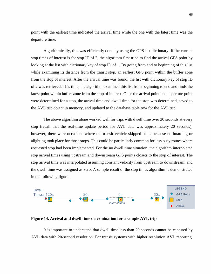
66
point with the earliest time indicated the arrival time while the one with the latest time was the
departure time.
Algorithmically, this was efficiently done by using the GPS-list dictionary. If the current
stop times of interest is for stop ID of 2, the algorithm first tried to find the arrival GPS point by
looking at the list with dictionary key of stop ID of 1. By going from end to beginning of this list
while examining its distance from the transit stop, an earliest GPS point within the buffer zone
from the stop of interest. After the arrival time was found, the list with dictionary key of stop ID
of 2 was retrieved. This time, the algorithm examined this list from beginning to end and finds the
latest point within buffer zone from the stop of interest. Once the arrival point and departure point
were determined for a stop, the arrival time and dwell time for the stop was determined, saved to
the AVL trip object in memory, and updated to the database table row for the AVL trip.
The above algorithm alone worked well for trips with dwell time over 20 seconds at every
stop (recall that the real-time update period for AVL data was approximately 20 seconds);
however, there were occasions where the transit vehicle skipped stops because no boarding or
alighting took place for those stops. This could be particularly common for less busy routes where
requested stop had been implemented. For the no dwell time situation, the algorithm interpolated
stop arrival times using upstream and downstream GPS points closets to the stop of interest. The
stop arrival time was interpolated assuming constant velocity from upstream to downstream, and
the dwell time was assigned as zero. A sample result of the stop times algorithm is demonstrated
in the following figure.
Figure 14. Arrival and dwell time determination for a sample AVL trip
It is important to understand that dwell time less than 20 seconds cannot be captured by
AVL data with 20-second resolution. For transit systems with higher resolution AVL reporting,

67
this algorithm will be able to capture smaller dwell times. Since excessive dwell times were often
the cause of significant delays and operational challenges for the surface transit system, especially
at major subways station, a 20-second resolution AVL data is sufficient for an application that
aims to characterizes the effects of delays and transit operational challenges.
5.3.4 Delay Calculations
In this thesis, transit schedule delay was defined as the difference between scheduled
arrival time and actual observed arrival time of a vehicle at a stop. As evident in the manner the
AVL trip route branch match and stop sequence was determined, the large portion of short turned
and temporary shuttle service on some of the transit routes introduced a few complications in delay
calculations. One of the complication was in the determination of the best-matched scheduled
arrival time. Another complication was to properly determine delay when there were missing
arrivals at a stop. Once these complications were addressed, best-matched schedule arrival times
were assigned for each actual observed arrival times. Using these assignments, the delay could be
determined using the difference between the scheduled and actual arrival times at a stop.
The simplest case in determining the best-matched scheduled arrival was for the first
observed stop times for each stop. For these cases, it was assumed that all previously scheduled
stop times were served. As such, there was no complication when dealing with the best-matched
scheduled arrival time and penalization of delay. In such circumstance, the best-matched scheduled
arrival time was simply the time closest to the actual arrival time. The delay was the time difference
between scheduled and actual arrival times. This is demonstrated in Figure 15.
Figure 15. Delay determination for all previous stop times served

68
A more general algorithm in determining delay accounted for missed stops, early arrivals,
and delay penalization, by keeping a detailed sequence of arrivals and their matches to schedule.
This algorithm first conducted a simple assignment of actual arrival times to schedule times based
on the smallest time difference. The simple assignment step found the scheduled arrival time
closest to actual arrival time.
Then, the next step assigned observed stop times with conflicted matches in a reversed
order. For instance, when two actual arrival times were both assigned to a single scheduled arrival
time in the simple assignment step, the earlier of the two was reassigned to an earlier schedule
arrival time match. This step was done in reverse order, from latest to earliest, to ensure the later
matches were not overwritten as only the earlier of the pair of the identical match were assigned
to an earlier match, effectively penalizing these instances of bunching. The reverse assignment
step was important for bunching vehicles where multiple vehicles may be serving the same
schedule arrival time but the earlier one of the vehicles may have missed a previously scheduled
arrival time, by being delayed and thus arriving at the same time as a later trip. By performing
reverse reassignment, the delay of these bunching vehicles was properly calculated.
After taking care of the complications regarding determining the best-matched schedule,
not all scheduled arrival times received a match with an actual arrival time. This could happen
with missed trips or short turned trips due to excessive delays on the route. This situation was
particularly common for congested streetcar routes. For instance, a vehicle could be delayed as it
progressed along its trip, eventually missing its own schedule arrival time at all its downstream
stops. To properly account for the delayed vehicle, delay for the vehicles with missed scheduled
arrival times was applied to only the first vehicle that missed scheduled stop times. In the
algorithm, missed delay penalization at a stop was applied to these missed schedule arrival times
for the situation demonstrated in Figure 16.

69
Figure 16. Delay determination for a trip with missed scheduled arrival times
The calculation of delay had a principal focus on the delay experienced from the customer’s
point of view. The trips following the one in Figure 16 were technically late as result of the missed
trip, if only a simple match to the schedule was made. However, this was not a realistic delay
estimation, because accumulative penalization on delays could produce artificial delays not
experienced by users. Instead, missed trip delays were accounted for using the missed stop delay
penalization algorithm, demonstrated in Figure 16. And from the customer’s point of view, the
vehicles arriving after the trip described in Figure 16 simply followed the later scheduled arrival
time. The way the algorithm deals with delay calculations after missed stop times situation is
demonstrated in Figure 17. Upon excessive delay from the earlier trip, the following trip served
the next sequence of scheduled arrival times at the downstream stop. This may result in some early
arrivals from the customer’s point of view. However, if the service ever fully recovered from such
delay, vehicles can eventually catch up to all of their schedule and the delay calculations were able
to reflect this by allowing a single schedule arrival time to be matched with more than one actual
arrival time, given all of the previous arrival times were served.
Figure 17. Delay determination for a trip following the trip with missed arrival times
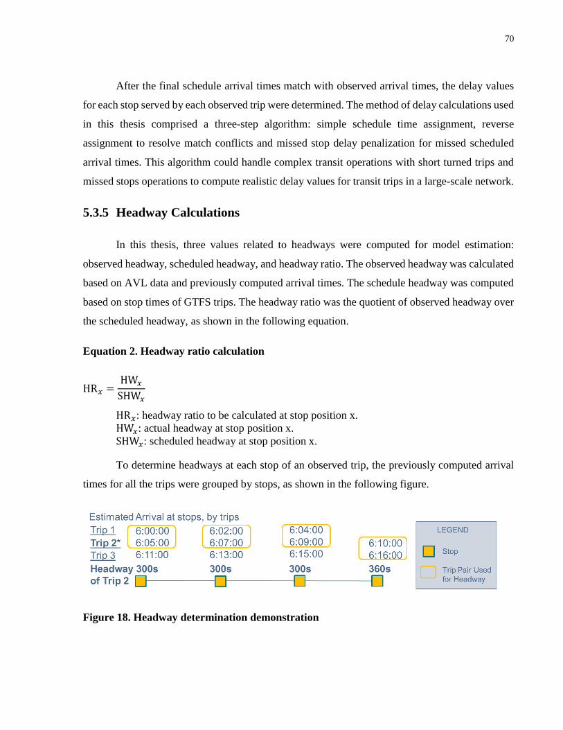
70
After the final schedule arrival times match with observed arrival times, the delay values
for each stop served by each observed trip were determined. The method of delay calculations used
in this thesis comprised a three-step algorithm: simple schedule time assignment, reverse
assignment to resolve match conflicts and missed stop delay penalization for missed scheduled
arrival times. This algorithm could handle complex transit operations with short turned trips and
missed stops operations to compute realistic delay values for transit trips in a large-scale network.
5.3.5 Headway Calculations
In this thesis, three values related to headways were computed for model estimation:
observed headway, scheduled headway, and headway ratio. The observed headway was calculated
based on AVL data and previously computed arrival times. The schedule headway was computed
based on stop times of GTFS trips. The headway ratio was the quotient of observed headway over
the scheduled headway, as shown in the following equation.
Equation 2. Headway ratio calculation
HR𝑥 =HW𝑥
SHW𝑥
HR𝑥: headway ratio to be calculated at stop position x.
HW𝑥: actual headway at stop position x.
SHW𝑥: scheduled headway at stop position x.
To determine headways at each stop of an observed trip, the previously computed arrival
times for all the trips were grouped by stops, as shown in the following figure.
Figure 18. Headway determination demonstration
71
When determining actual headways, the AVL trip ID of the stop time values and calculated
headways were tracked so the actual headway values were organized by trips, rather than by stops.
This was particularly important for cases where there were insufficient stop times at a stop, for
example when only one trip serviced a stop. When headway for a stop in a trip cannot be computed
using observed arrival times, the headways were interpolated based on the headways and stop
distances at the closest upstream and downstream stops with computed headway values. The
interpolation of headway was based on weighted average of headway based on distance from start
stop, as detailed by the following equation.
Equation 3. Headway interpolation using upstream and downstream headways
HW𝑥 = HWupstream, j +(Dx − Dupstream, j)
(Ddownstream, i − Dupstream, j)(HWdownstream, i − HWupstream, j)
HW𝑥: missing headway to be calculated at stop position x.
Dx: distance from start stop at stop position x.
HWupstream, j: upstream headway at stop position j
HWdownstream, i: downstream headway at stop position i
Dupstream, j: distance from start stop at stop position j
Ddownstream, i: distance from start stop at stop position i
The calculation of schedule headway was similar to the calculation of observed headway
except the stop times used were from the GTFS trip stop times during the period of interest. Using
the calculated observed headway and scheduled headway, the headway ratio can be obtained.
These values were important in characterizing the effect of transit congestion during operations
and could indicate the occurrence of transit vehicle bunching.
5.3.6 Previous Speeds
For the determination of previous running speeds for each link-based observation, it was
important to keep track of the order of trip arrivals at stops. For this thesis, the previous trip speed
at the current link (previous trip speed) and the previous link speed for the current trip (previous
link speed) were used. The previous trip speed accounted for the time lag effect of travel speed,
72
while the previous link speed accounted for the spatial lag effect of travel speed. The previous
speed attributes ensured the travel time prediction was both realistic and reasonable and were not
dependent on operational and link attributes alone.
To keep track of the order of previous trip speeds so they could be retrieved quickly, an
object “PreviousTripIDByTripIDByStopID” was constructed and used to query previous trip
speeds. For the retrieval of previous link speed, the current trip ID and the previous stop ID was
used to query previous link speed.
5.3.7 Conversion and Initialization Link Data
With transit operational attributes found for each AVL trip and stop within the trip, the trip
based data could be converted to link based data. Stop-to-stop based transit travel was established
in the framework of this thesis as it provided an appropriate level of detail for transit simulation.
Use of the link based data and the attributes from map matching allowed the incorporation of
transit operational attributes, disruption attributes, link attributes, and route attributes.
To perform the conversion to link data, links with unique names were created using the
start stop code and end stop code, separated by an underscore (i.e.: “3271_8373”). After these
unique link names were created, an algorithm went through all the AVL trips, reading the
processed data organized in sequence by start stop ID and populating all the values of transit
operational attributes previously calculated. The transit operational attributes at the start stop are:
stop time, dwell time, link distance (also was a link attribute), running speed, delay, headway,
previous speeds. The link attributes identified were linkID (with start and end stop codes), link
distance, and scheduleID. Additional unprocessed attributes were initialized so they could be
computed in the next steps of the data processing algorithm.
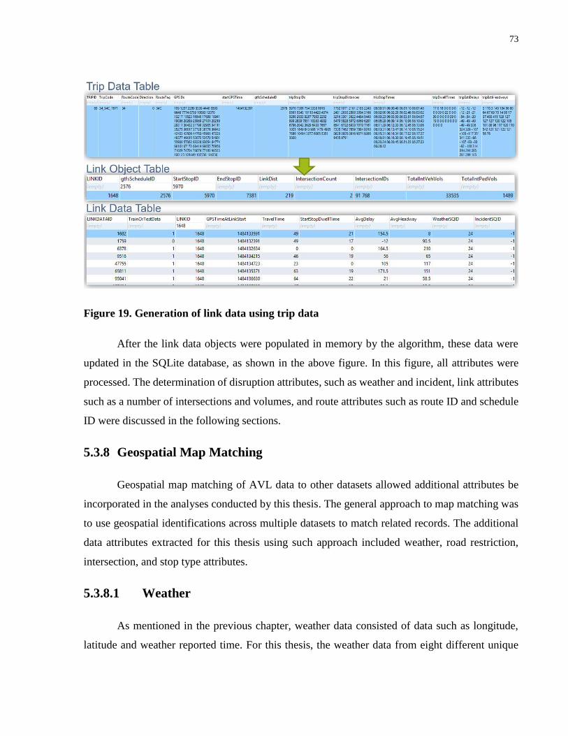
73
Figure 19. Generation of link data using trip data
After the link data objects were populated in memory by the algorithm, these data were
updated in the SQLite database, as shown in the above figure. In this figure, all attributes were
processed. The determination of disruption attributes, such as weather and incident, link attributes
such as a number of intersections and volumes, and route attributes such as route ID and schedule
ID were discussed in the following sections.
5.3.8 Geospatial Map Matching
Geospatial map matching of AVL data to other datasets allowed additional attributes be
incorporated in the analyses conducted by this thesis. The general approach to map matching was
to use geospatial identifications across multiple datasets to match related records. The additional
data attributes extracted for this thesis using such approach included weather, road restriction,
intersection, and stop type attributes.
5.3.8.1 Weather
As mentioned in the previous chapter, weather data consisted of data such as longitude,
latitude and weather reported time. For this thesis, the weather data from eight different unique
74
weather stations were collected and loaded for processing. These stations were: Agincourt,
Downsview, Downtown Toronto, Etobicoke, Rexdale, Scarborough Station, Thornhill, and
Vaughan. These weather stations provided a distributed and complete coverage of the Toronto
Region that the Toronto Transit Commission serviced.
For each link data, an algorithm determined the nearest weather station to the link based
on the distances between the link and the weather station. Then, the data from that weather station
that was closest in time to the link data time was assigned to the link data. Once all the link data
within all the link objects were updated, in memory and in the database table, with weather data
via the assignments of weather data ID (WeatherSQID), weather information such as temperature,
humidity, wind speed, rain precipitation, and snow precipitation could be retrieved for each link
data quickly when exporting features (variables).
5.3.8.2 Road Restriction
Road restriction records had time fields and location fields. Each record of road restriction
provided the start time, end time and last updated time of the restriction, as well as the as longitude,
latitude of the road restriction event. Using the geospatial fields, the road restriction record event
that existed on a link data record was determined. The road restriction data were collected for the
entire City of Toronto and were maintained by the City of Toronto Transportation Services and
Open Data Team. This dataset provided a complete coverage for the areas that the Toronto Transit
Commission serviced.
Unlike weather data which used proximity for the geographical match, road restriction data
record must be on the link to be considered a valid record for that link. To check this, a buffer
width of 25 metres along the links was used to determine if the road restriction record falls
anywhere on the link. If a road restriction record falls within the link, its “IncidentSQID” was
assigned to that link; if no record was found for that link, then the “IncidentSQID” was set to
negative one (-1) to indicate no restrictions. In addition to making sure the restriction record was
geographically on the link, the link data time must fall between the start and end time of the
75
restriction for the restriction as well, for it to be assigned to the link. The final step of road
restriction matching was to update the link data table in the SQLite database.
5.3.8.3 Intersection Attributes
The intersection and signals data from Open Data Toronto provided the geographical
locations of traffic signals, flashing beacons, and pedestrian crossovers, as well as the latest
pedestrian and traffic volumes for over 2,000 intersections. (City of Toronto, 2017b, 2017c).
Before matching, four separate XML files were loaded into memory into a list of common type
“SSINTNXSignalDataTable” with no duplicate intersections. Each intersection contained fields
such as longitude and latitude, while some intersections contained additional fields such as street
names, signal types (TSP, Actuated, and Adaptive) and volumes (8-hour pedestrian and traffic).
Similar to the procedure used for road restriction data, the algorithm for intersection
attributes searched for intersections falling on the link by checking if any of the intersection was
on the link, with a 25 metres buffer width. Only the intersections within the start and end stops of
the link was added to a list of intersection IDs for the link object.
In addition to keeping track of the list of intersections that were on each link, some
attributes related to intersections were also determined. The following list describes the attributes
found, their variable name (in bracket), and any additional sub-procedures required to obtain them
(after the colon):
• stop types (“far-side” and "near-side"): to determine if the stop type of the start stop or
end stop was far-sided or near-sided, the algorithm checked if there were any intersection
during the search near the start and end stops. The tolerance for the distance between the
intersection and the potential stop was 50 metres. For instance, if the algorithm found an
intersection 30 metres downstream of the end stop, then the end stop was found as a near-
sided stop. Conversely, if the algorithm found an intersection 30 metres upstream of the
start stop, then the start stop was determined as a far-side stop.

76
• the number of signalized intersections (“Num_Intxn”): the number of signalized
intersections was computed by going over the list of intersections found to be on the link
and counting the number of intersections that were signalized intersections.
• the number of TSP equipped intersections (“Num_TSP_equipped”): the number of
TSP intersections was determined by going over the list of intersections found to be on the
link and counting the number of intersections that were TSP intersections.
• the number of pedestrian intersections (“Num_PedCross”): the number of pedestrian
intersections was determined by going over the list of intersections found to be on the link
and counting the number of intersections that were pedestrian crossing intersections.
• the number of left turns made by the transit vehicle at a signalized intersection
(“Num_VehLtTurns”): left turns made by transit vehicles were detected when there were
changes in the direction the path connecting start and end stop in the anti-clockwise
direction. Such change needed to be accounted for to properly determine whether a point
was on the link.
• the number of right turns made by the transit vehicle at an intersection
(“Num_VehRtTurns”): right turns made by transit vehicles were detected when there
were changes in the direction the path connecting start and end stop in the clockwise
direction.
• the number of through movements made by the transit vehicle at an intersection
(“Num_VehThroughs”): no turns detected because the change in direction within the path
connecting start and end stop is minimal (<45 degrees).
• average vehicle volume on the link (“AvgVehVol”): the average vehicle volumes across
all intersection volume counts within the link. If there was no volume record for vehicles
at an intersection, that volume was ignored.

77
• average pedestrian volume on the link (“AvgPedVol”): the average pedestrian volumes
across all intersection volume counts within the link. If there was no volume record for
pedestrians at an intersection, that volume was ignored.
• is streetcar route (“IsStreetcar”): based on route properties and route code of the link
object, the route characteristics were updated to the link object during the geospatial map
matching step.
• dedicated right of way (“IsDedicatedROW”): based on route properties and route code
of the link object, the route characteristics were updated to the link object during the
geospatial map matching step.
Using the algorithm that performed geospatial map matching with intersection data and
link object data, additional attributes about the weather, road restrictions, stops, intersections, and
routes were extracted. The technique of geospatial map matching was successfully applied to
multiple data sources to enrich the breadth of attributes related to link data and link objects, which
allows for a more descriptive travel time model.
5.4 Data Export
After data processing has been completed, link data with a set of variables could be
exported for model estimation of travel time models. Depending on the model specifications of
the travel time model, the list of variables needed for model estimation may differ. Based on the
information available in our processed dataset, the following table provides lists of possible
variables that were exported into a file with common-separated values (CSV) format.

78
Table 6. List of possible variables, attributes, by data sources
Data Source Attributes List of Possible Variables
AVL Observed Arrival
Times and Dwell
Times at Stops
RunningSpeed, DwellTime, LinkDist,
PrevLinkRunningSpeed, PrevTripRunningSpeed,
TerminalDelay, Delay, Headway, ScheduleHeadway,
HeadwayRatio, Day, Time_mins
GTFS Schedule Arrival
Times
RouteCode, GtfsScheduleID, LinkName, StopSeq,
StartStopID,
Weather Weather
Locations and
Conditions by ID
TotalPptn
Road
Restriction
Road Restriction
Locations and
Conditions by ID
HasIncident
Intersection
and Signal
Data
Intersection
Locations and
Properties by ID
Num_VehLtTurns, Num_VehRtTurns,
Num_VehThroughs, Num_TSP_equipped,
Num_PedCross, AvgVehVol, AvgPedVol,
IsStartStopNearSided, IsEndStopFarSided
Route
Properties
(Customize
Route
Information)
Streetcar or Bus,
and Shared or
Dedicated Right
of Way
IsStreetcar, IsSeparatedROW

79
5.5 Summary
This chapter demonstrated an automatic data processing procedure that extracted attributes
from multiple sources of open data, which could be used to generate descriptive variables and
features for model estimation of a large-scale transit network. There were four major steps
involved in data processing. Data loading allowed for the program to perform the operations in
memory. AVL data preprocessing eliminated erroneous data. Trip data processing formed AVL
trips, computed arrival and dwell times, computed delays, computed headways, found previous
speeds, and performed geospatial map matching to enrich link data attributes. Finally, data export
converted processed data attributes into specific link data variables. Using the possible list of
variables, different types of travel time models were estimated and evaluated.

80
Chapter 6
Model Estimation
Once a list of defined variables had been obtained from data processing, they were used to
estimate models to represent transit travel times. While it was common for previous studies to use
terminal-station-based and time-point-based segments to model transit travel times, these methods
are less flexible when applied to simulation since the ability to generate transit vehicle arrival
patterns at only key transit stops has limited simulation applications. This thesis examines the
potential of representing travel times for stop-based links using open data sources, namely GTFS,
AVL, weather, road restriction and intersection data. This thesis explores various regression
modelling methods to model running speed and estimate an appropriate distribution model for
dwell time.
The decision to model running speed and dwell time separately had a few major benefits.
Firstly, since we know that dwell time was the result of passenger boarding and alighting at stops
rather than the variables we have available such as weather, road restrictions, number of
intersections at the link, it was more sensible to exclude dwell time from being characterized by
the variables in the running speed model. While it is true that passengers boarding and alighting
can be affected by weather and road restriction conditions, without detailed passenger demand data
at each stop, the effects of weather and road restriction conditions on passenger boarding and
alighting cannot be properly characterized. This assumption needs to be addressed in future studies
and extensions of the modelling framework presented by this thesis. Secondly, separating dwell
time enabled this thesis to evaluate the effectiveness of distribution-based dwell time models at
representing transit travel times accurately. Finally, separation of dwell time allows future studies
to extend this data-driven modelling technique by investigating the use of APC or AFC data to
model the effect of passenger demand on dwell times, enabling high fidelity data-driven transit
simulations. The rest of this chapter presents a detailed procedure to estimate dwell time and
running speed models to support the simulation of a data-driven mesoscopic transit model.

81
6.1 Running Speed Model
This thesis used four main steps to complete model estimations of running speed models.
The processed data was first loaded into R workbench, formatted according to data type, and split
into training and test data. Then, the variables were defined and the model type was assigned. The
most computationally intensive step was model training. The model training step used R packages
to estimate running speed models. Finally, the estimated models were used to generate predictions
and these predictions were evaluated against test data. Figure 20 illustrates the four steps of model
estimation.
Figure 20. Model estimation process flow for running speed model
6.1.1 Data Retrieval
The data retrieval step involved the validation of data types and splitting the data table into
training and test data. The processed data was saved in a common separated values (CSV) file with
data column names. These data were first loaded into the R workbench using the “fread” function
from “data.table” package in R. When performing model estimations with R, it was important to
specify the correct data type of each column. For example, the route number variable (RouteCode)
was recognized as an integer value by default, but it should be a categorical value. This was
particularly important because, for many modelling methods, categorical variables were treated
differently when performing estimations. After the data were loaded and the data types validated,
Data Retrieval
•Validate Data Types
•Split into training and test data
Model Specifications
•Define target and predictors
Model Training
•Assign model type
•Assign model parameters
Model Prediction and
Evaluation
82
using the “TrainingOrTest” variable field included in the CSV and the split function, separate
training data and test data tables were loaded into the R workbench.
6.1.2 Model Specifications
To estimate meaningful models, the list of variables required that are dependent on the
specific use case and functional requirement of the model need to be specified. This study
established two potential use cases for demonstration. The first was a basic analysis of a transit
route, and the second was an advanced analysis of the entire transit network. The route level model
was designed to account for temporal effects, transit operational characteristics, and basic link
characteristics. The set of variables required were mainly based on attributes extracted from AVL
and GTFS data only. On the other hand, the advanced analysis model required additional link and
route characteristics. With larger sample sizes, weather and road restriction effects on travel time
could be explored as well.
Many variables were used to model running speeds in the route level basic model. To
capture the effect of temporal factors on running speed, the variables day of the week (Day), as
well as the time of the day (Time_mins), were used for the route level model. In addition, headway,
delay, previous link travel speed, and previous trip travel speed variables were used to account for
the effects of transit operational characteristics. Finally, link characteristics, such as link distance
or link name, were used to model the effects of link characteristics.
Due to the variability between different transit routes, the network level advanced model
for running speed required additional variables to account for the spatial variation of links and
routes. With additional link characteristics such as stop locations, link distance, left and right turns
made by transit vehicles, as well as vehicle volumes and pedestrian volumes, the network level
model could account for the variation due to link characterises across the transit network.
Furthermore, the use of the “hasIncident” (road closure incidents) and “totalPptn” (precipitation)
was possible with the network level model since the data was sufficient in geographical scale to
cover areas with different incident occurrences and total precipitation.
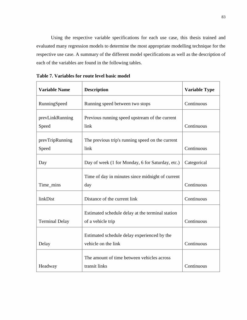
83
Using the respective variable specifications for each use case, this thesis trained and
evaluated many regression models to determine the most appropriate modelling technique for the
respective use case. A summary of the different model specifications as well as the description of
each of the variables are found in the following tables.
Table 7. Variables for route level basic model
Variable Name Description Variable Type
RunningSpeed Running speed between two stops Continuous
prevLinkRunning
Speed
Previous running speed upstream of the current
link Continuous
prevTripRunning
Speed
The previous trip's running speed on the current
link Continuous
Day Day of week (1 for Monday, 6 for Saturday, etc.) Categorical
Time_mins
Time of day in minutes since midnight of current
day Continuous
linkDist Distance of the current link Continuous
Terminal Delay
Estimated schedule delay at the terminal station
of a vehicle trip Continuous
Delay
Estimated schedule delay experienced by the
vehicle on the link Continuous
Headway
The amount of time between vehicles across
transit links Continuous
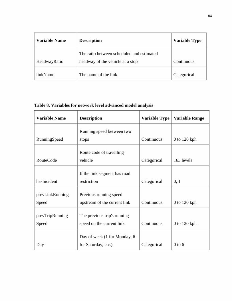
84
Variable Name Description Variable Type
HeadwayRatio
The ratio between scheduled and estimated
headway of the vehicle at a stop Continuous
linkName The name of the link Categorical
Table 8. Variables for network level advanced model analysis
Variable Name Description Variable Type Variable Range
RunningSpeed
Running speed between two
stops Continuous 0 to 120 kph
RouteCode
Route code of travelling
vehicle Categorical 163 levels
hasIncident
If the link segment has road
restriction Categorical 0, 1
prevLinkRunning
Speed
Previous running speed
upstream of the current link Continuous 0 to 120 kph
prevTripRunning
Speed
The previous trip's running
speed on the current link Continuous 0 to 120 kph
Day
Day of week (1 for Monday, 6
for Saturday, etc.) Categorical 0 to 6

85
Variable Name Description Variable Type Variable Range
Time_mins
Time of day in minutes since
midnight of current day Continuous 0 to 86,400 mins.
linkDist Distance of the current link Continuous 0 to 11,600 m
Terminal Delay
Estimated schedule delay at the
terminal station of a vehicle
trip Continuous -1000 to 3000 s
Delay
Estimated schedule delay
experienced by the vehicle on
the link Continuous -1000 to 3000 s
Headway
The amount of time between
vehicles across transit links Continuous 0 to 3000 s
HeadwayRatio
The ratio between scheduled
and estimated headway of the
vehicle at a stop Continuous 0 to 10
totalPptn
Total precipitation reported at
the nearest weather station to
current link Continuous 0 to 10 mm
num_VehLtTurns
Number of left turns by the
transit vehicle Categorical 0 to 2
num_VehRtTurns
Number of right turns by the
transit vehicle Categorical 0 to 3

86
Variable Name Description Variable Type Variable Range
num_VehThroughs
Number of through movements
at intersections made by the
transit vehicle on the link Categorical 0 to 14
num_TSP_equipped
Number of TSP equipped
intersections on the link Categorical 0 to 6
num_PedCross
Number of pedestrian
crossings on the link Categorical 0 to 3
avgVehVol
Average vehicle volume of the
link Categorical 0 to 20,000
avgPedVol
Average pedestrian volume of
the link Categorical 0 to 10,000
isStartStopNearSided If start stop is near sided Categorical 0 or 1
isEndStopFarSided If end stop is far sided Categorical 0 or 1
isStreetcar
If the route on the link a
streetcar route Categorical 0 or 1
isSeparatedROW
If the link on the route
separated right-of-way Categorical 0 or 1
linkName The name of the link Categorical 9267 levels
87
6.1.3 Model Training
After training data, test data, and variable specifications were loaded into the R workbench,
specific models could be trained using corresponding statistics and machine learning packages in
R. This thesis investigated 5 types of regression models for the estimation of running speeds:
multiple linear regression, support vector machine, linear mixed effect regression, regression tree,
and random forest. The followings sections present the theory (model form and estimation
technique), key assumptions, and applications (statistical package used and parameter
specifications) for each model.
6.1.3.1 Multiple Linear Regression
Multiple linear regression (MLR) relates the target variable, y, with multiple predictor
variables Xi using a linear combination of the predictor variables (Young, 2017). The relationship
between the target variable and predictor variable can be expressed as:
Equation 4. Functional form of MLR models
𝑦 = 𝛽0 + 𝛽1𝑥1 + 𝛽2𝑥2 + ⋯ + 𝛽𝑖𝑥𝑛 + 𝜖 = 𝛽𝑋𝑇 + 𝜖
𝑦: response/target variable
𝛽: estimated coefficients for predictor variables,
𝑋: predictor variables,
𝜖: residuals
Estimation of MLR 𝛽𝑖 coefficients is done by minimizing the sum of squared errors for the
sample observations, where m is the number of sample observations. This is also known as

88
ordinary least square estimation where the variance of the model is minimized. The objective
function to be minimized can be expressed as follows:
Equation 5. Objective function of MLR models
min [1
2𝑚∑(𝜖𝑗)
2𝑚
𝑗=1
]
where the residual is 𝜖 = 𝑦𝑖 − �̂�𝑖, the difference between observed and predicted values
Assumptions
There are four fundamentals assumptions associated with MLR: linear relationship,
normally distributed errors, homoscedasticity, and independence. The linear relationship
assumption is often a reasonable one, and in the case where the specific relationship is known,
such as 𝑙𝑛(𝑦) = 𝑥, or 𝑦 = 𝑥2, etc., transformation can usually be applied. In the context of
transit travel times, determining and specifying the type of nonlinear relationship is often difficult
due to varying conditions and presence of random variation in our data. This variation generates
random errors which are accounted for by the residual term. In MLR, the residuals are assumed to
be normally distributed. This is a reasonable assumption for modelling with large data sets for
continuous variables, and the assumption can be evaluated by examining the distribution of
residuals. Thirdly, homoscedasticity means that the standard deviations of the normally distributed
errors must not vary across the ranges of the predictor variables 𝑥𝑖. This implies that the normally
distributed errors are distributed in the same way for y regardless of the value of the predictors.
Finally, MLR assumes independence between predictor variables, which requires the predictor
variables to have zero covariance from one another. This is often an issue in modelling since many
of the variables we specify often are correlated with one another. In this study, vehicle and
pedestrian volumes are certainly correlated. Some variables that may correlates with one another
may be headway and delay, as well as the types of vehicle movements at intersections and link
distance. MLR can account for dependence between variables with interaction terms; however, if

89
the effects of the correlations are weak and the number of correlated variables are large, interaction
term can impose heavy computational requirements when estimating model parameters.
Applications
This thesis used the MASS package from R to estimate MLR models (Ripley et al., 2017).
A formula and training data were used as input for MLR model estimation. The formula consisted
of the target variable “RunningSpeed” and a list of predictor variables listed in Table 7 and Table
8, as part of the model specification. The training data set was obtained at the end of the data
retrieval step. MLR model does not contain any parameters that need to be tuned or specified since
the only variable in its objective function is the residual.
For this thesis, interaction terms were not considered due to the relatively large number of
interaction variable terms that needed to be tested, which would increase model training times
exponentially. For instance, to fully test interaction effects between all k=20 variables, given that
the number of interaction parameters is equal to 2k – k – 1, the number of interaction effect
variables would be over a million. It would be even more difficult to apply given about half the
variables used in this thesis are categorical variables which would require dummy variables that
would further increase the number of interaction variable parameters needed.
6.1.3.2 Support Vector Machine
Support vector machine is a machine learning algorithm that derived its ability to perform
classification and regression from the idea of hyperplane margin optimization and kernel functions
to model highly nonlinear relationships (Hsu, Chang, & Lin, 2016).
Support vector machine finds an optimal hyperplane that maximizes the separation or
“margin” between groups of data with different properties. This is achieved by identifying a group
of linearly separable data points on the edges of a certain label and making them the support
vectors. Figure 21 shows how support vector machine separates two groups of data (blue/small

90
and red/big points) using the idea of edge vectors supporting the margin with maximum separation
ε. Such optimal hyperplane maximization uses the objective function identified in Equation 6.
Using the idea of the optimal hyperplane, support vectors are used as the model for classification
and regression in support vector machine.
Figure 21. Separating and classifying data with support vector machine
Equation 6. Objective function of support vector machine
min [𝐶 ∑ 𝜉𝑖
𝑙
𝑖=1
+1
2𝑤𝑇𝑤], 𝜉𝑖 ≥ 0
where 𝑤 is normal vector to the hyperplane,
C is constant on the error terms (regularization parameter),
𝑙 is sample size, and
𝜉𝑖 are estimation errors terms (Cortes & Vapnik, 1995).

91
Traditionally, the modelling of nonlinear relationships is computationally expensive due to
a large number of polynomial terms in the higher dimensional functions when modelling higher
order variables. To deal with such issue, support vector machine performs kernel tricks obtain the
dot product of the transformed vectors without needing a higher dimensional function. Support
vector machine achieves this with a kernel function. Some common kernel functions are the linear
kernel, radial basis function kernel, and polynomial kernel (Hsu et al., 2016). The use of kernels
allows the objective function to be evaluated efficiently to obtain a set of support vectors that
minimizes the objective function.
Equation 7. linear kernel
𝐾(𝑥𝑖, 𝑥𝑗) = 𝑥𝑖𝑇𝑥𝑗
where 𝑥𝑖𝑇 is a transposed vector of one data point
where 𝑥𝑗 is a transposed vector of another data point
Equation 8. Radial basis function (RBF) kernel
𝐾(𝑥𝑖, 𝑥𝑗) = exp (−𝛾‖𝑥𝑖 − 𝑥𝑗‖2
)
where the hyperparameter gamma is 𝛾 > 0
Equation 9. Polynomial kernel
𝐾(𝑥𝑖, 𝑥𝑗) = (𝛾𝑥𝑖𝑇𝑥𝑗 + 𝑟)
𝑑
where the hyperparameter gamma is 𝛾 > 0
r is the polynomial degree

92
To adapt support vector machine for regression, support vector regression uses a ε-
insensitive error measure where low error values are ignored while larger error contributes linearly
to the absolute residual greater than a constant ε, as shown in (Hastie, Friedman, & Tibshirani,
2008). This makes the fitting less sensitive to outliers (Hastie et al., 2008). The soft margin
hyperplane and kernel property are not unique to classification and they have been demonstrated
in past studies to be integral to the properties of support vector regression (Smola & Schölkopf,
2004).
Equation 10. Support vector machine ε-insensitive loss function for regression
𝜉𝜀 = |𝑟| − 𝜀
where error penalization is |𝑟| ≥ 𝜀
Assumptions
While support vector machine is a much more flexible algorithm than MLR, it does require
the independent and identically distributed (I.I.D.) assumption for the error term to hold true
(Balakrishna, Raman, Trafalis, & Santosa, 2008). Unlike MLR, support vector machine can
account for the correlation between predictor variables with kernel functions. Because kernels can
implicitly map higher order combinations of variables, nonlinear as well as correlated relationships
can be modelled by support vector machine. Depending on the kernel chosen, the degree and
specification of the interaction terms can be different. A linear kernel support vector machine is
similar to ridge regression where the linear combination of variables are modelled, while
polynomial kernel support vector machine also maps the combination of variables in higher order
(Marsupial, 2012). In addition, the radial basis function kernel is formed by an infinite sum over
polynomial kernels; therefore, it can be used as a universal kernel approximator to represent any
decision boundary and nonlinear shapes (Bernstein, 2015). Consequently, radial basis function
kernel is preferred over the polynomial kernel.
93
Applications
This thesis used the “e1071” and “liquidSVM” packages to estimate support vector
machine models in R (Meyer et al., 2017; Steinwart & Thomann, 2017). A formula, the type of
kernel function, as well as the hyperparameters associated with the kernel function need to be
specified for the estimation of support vector machine models. Hyperparameters such as the
regularization parameter (C), kernel function parameters (𝛾, 𝑑), and loss function parameter (𝜀)
should also be determined through k-fold cross-validation, then specified for the final support
vector machine model.
A k-fold cross validation procedure using a grid-search method was used to find the most
suitable set of 𝐶 and 𝛾 parameters. The k-fold cross validation procedure divides training data into
k number of subsets and trains the model sequentially by each subset (Hsu et al., 2016). This
method of finding 𝐶 and 𝛾 prevents overfitting while minimizing the root mean squared error (Hsu
et al., 2016). A common 𝜀 value of 0.001 was used since it was reasonable to exclude very small
estimation errors (Hsu et al., 2016).
This thesis used support vector machine to investigate if the modelling of nonlinear
relationships using different kernels improved model performance. Through our preliminary
analysis, we compared linear kernel and radial basis function kernel. We eliminated polynomial
kernel from our preliminary analysis due to its computational complexity and potential numerical
difficulties associated with the polynomial kernel. The polynomial kernel has a larger number of
hyperparameters which would require exponentially more computing time when selecting these
hyperparameters through cross-validations (Hsu et al., 2016). Also, the polynomial kernel may
generate zero or infinity kernel values for larger degrees (Hsu et al., 2016). Consequently, a
preliminary analysis between linear kernel and radial basis function kernel was done on a group
of 25 routes, and the results of RMSE can be found in Table 9.

94
Table 9. Comparing linear and RBF kernels for support vector machine
Route RMSE for Linear Kernels* (kph) RMSE for RBF Kernels* (kph)
5 12.5 13.7
6 13.0 11.6
7 13.2 12.8
8 17.4 12.7
9 12.7 13.8
11 21.4 13.9
12 16.2 21.8
14 18.0 10.1
15 17.1 13.9
16 14.7 14.5
17 17.1 14.8
20 15.2 13.3
21 15.5 15.0
22 8.3 10.0
23 12.8 11.8
24 18.8 16.1
25 16.8 13.6
26 14.7 15.0
28 13.8 12.6
29 11.4 12.6
30 14.9 14.5
31 19.0 12.2
32 16.5 14.4
33 7.9 10.8
Average 15.0 13.6
Total Runtime for Routes (min.)
10 120
Runtime per Route (min.)
0.42 5.0
* RMSE: root mean square error
Based on the result of the preliminary analysis of support vector machine kernel functions,
RBF can reduce the error of the estimate further for route level models. As such, a k-fold cross
validation procedure with RBF kernel was used in estimating support vector machine models.

95
In addition to selecting kernel function, another issue related to the application of support
vector machine is its limitations when applying it to large datasets. Since finding an optimal
solution to support vector machine requires dot products of all the feature vectors as well as
optimizing the objective function, the computational time complexity of support vector machine
is O(n3), where n is the number of samples (C. Hu, Zhou, & Hu, 2014). Because the computational
time with conventional support vector machine grows exponentially with training sample size,
support vector machine may run into difficulties for network level models with a very large sample
size.
6.1.3.3 Linear Mixed Effect Model
Linear mixed effect models are an extension of MLR model which address the issue of
heteroscedasticity that is often present in repeated measurements and sampling. The linear mixed
effects model does this by modelling random effect variables, in addition to fixed effect variables
that were modelled by MLR. Homoscedasticity refers to the assumption that the distribution of
error term does not vary across different values of fixed effect variables. The use of random effect
variables accounts for heteroscedasticity by varying the intercept and/or slope of the linear function
over different levels of the random effect variable (Seltman, 2016). The mixed-effect linear model
is mathematically expressed by the following equation.
Equation 11. Functional form of linear mixed effects models
𝑦 = 𝛽𝑋𝑇 + 𝑢𝑍𝑇 + 𝜖
𝑦: response/target variable
𝛽: estimated coefficients for fixed-effect predictor variables,
𝑋: fixed-effect predictor variables,
𝑢: estimated coefficients for random-effect predictor variables,

96
𝑍: random-effect predictor variables,
𝜖: residuals
The estimation of linear mixed effects model 𝛽 and 𝑢 coefficients requires the joint
likelihood distributions of the fixed and random effect variables to be maximized. As such, the
objective function for the log-joint distribution of (y, u) is can be expressed as follows (Gumedze
& Dunne, 2011), assuming 𝑢 and 𝑦 represent a joint Gaussian distribution with the following
mean and covariance.
Equation 12. Mean and covariances of u and y for linear mixed effects model
[𝑢𝑦] ~𝑁 (𝑚𝑒𝑎𝑛 [
0𝛽𝑋
] , 𝑐𝑜𝑣 [ 𝐺 𝐺𝑍′𝑍𝐺 𝐻
])
where the variance-covariance of y is: 𝑣𝑎𝑟(𝑦) = 𝜎2(𝑍𝐺𝑍′ + 𝑅) = 𝜎2(𝐻),
𝑍 is the design matrix for random-effect variables,
𝐺 is the known component of random-effect variables,
R is the known component of residuals.
It was shown in the literature that the above join Gaussian distribution can be expressed as follows
(Gumedze & Dunne, 2011).
Equation 13. Log joint distribution of y and u for linear mixed effects model
𝑢~𝑁(0, 𝜎2(𝐺))
𝑦|𝑢~𝑁(𝛽𝑋 + 𝑢𝑍, 𝜎2(𝑅))
log 𝑓(𝑦, 𝑢) = log 𝑓(𝑦|𝑢) + log 𝑓(𝑢) =1
2𝜎2{𝑢′(𝑍𝑅−1𝑍′ + 𝐺−1)𝑢 − 2(𝑦 − 𝑋𝛽)′𝑅−1𝑍𝑢}
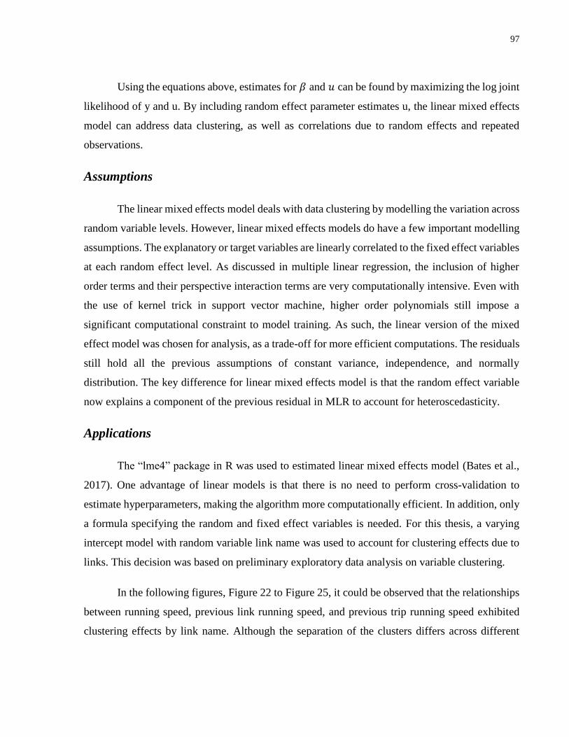
97
Using the equations above, estimates for 𝛽 and 𝑢 can be found by maximizing the log joint
likelihood of y and u. By including random effect parameter estimates u, the linear mixed effects
model can address data clustering, as well as correlations due to random effects and repeated
observations.
Assumptions
The linear mixed effects model deals with data clustering by modelling the variation across
random variable levels. However, linear mixed effects models do have a few important modelling
assumptions. The explanatory or target variables are linearly correlated to the fixed effect variables
at each random effect level. As discussed in multiple linear regression, the inclusion of higher
order terms and their perspective interaction terms are very computationally intensive. Even with
the use of kernel trick in support vector machine, higher order polynomials still impose a
significant computational constraint to model training. As such, the linear version of the mixed
effect model was chosen for analysis, as a trade-off for more efficient computations. The residuals
still hold all the previous assumptions of constant variance, independence, and normally
distribution. The key difference for linear mixed effects model is that the random effect variable
now explains a component of the previous residual in MLR to account for heteroscedasticity.
Applications
The “lme4” package in R was used to estimated linear mixed effects model (Bates et al.,
2017). One advantage of linear models is that there is no need to perform cross-validation to
estimate hyperparameters, making the algorithm more computationally efficient. In addition, only
a formula specifying the random and fixed effect variables is needed. For this thesis, a varying
intercept model with random variable link name was used to account for clustering effects due to
links. This decision was based on preliminary exploratory data analysis on variable clustering.
In the following figures, Figure 22 to Figure 25, it could be observed that the relationships
between running speed, previous link running speed, and previous trip running speed exhibited
clustering effects by link name. Although the separation of the clusters differs across different

98
routes and between different links, it was evident that in general, there was a pattern of clustering
emerging whereby each link occupied a region of the graph space. For example, for route 192, link
“14092_14278” (from Pearson Terminal 1 to Pearson Terminal 3) had more sparse changes in
speed from previous link and trips than its link “2148_14719” (from Dundas St W at the East Mall
Cres to Kipling Station), where the changes in speed from previous link and trip is minimal. For
streetcar routes such as 504, clustering effect by link existed as well. While link “11596_11596”
(Roncesvalles Ave at Queen St W to Roncesvalles Ave at Queen St W North) occupied the lower
speed regions, link “4573_14992” (Roncesvalles Ave at Galley Ave to Roncesvalles Ave At
Marion St South Side) occupied higher speed regions.
Figure 22. Clustering pattern for links for route number 192

99
Figure 23. Clustering pattern for links for route number 504
Figure 24. Clustering pattern for links for route number 196

100
Figure 25. Clustering pattern for links for route number 510
6.1.3.4 Regression Trees
A regression tree is a nonparametric modelling technique based on classification and
regression trees – CART. It uses the idea of node splitting to partition data into different nodes,
forming a decision tree which models the outcome by applying the node splitting decisions based
on predictor variable values. The advantage of regression tree is that it can determine the variables
that were most important in generating predictions, thus using those variables to generate
predictions efficiently. To perform node splitting, regression tree uses an impurity measure for
each node (Equation 14) to maximize the decrease in the change of impurity because of the node
split (Equation 15) (Berk, 2008). The objective of building trees is to maximize the decrease in
impurity with each node construction, thus resulting in a tree with minimum impurity.
Equation 14. Impurity of a node
𝑖(𝜏) = ∑(𝑦𝑖 − �̅�(𝜏))2

101
where 𝜏 is a node on the tree,
�̅�(𝜏) is the mean of the node, which is also the prediction value
Equation 15. Change in impurity due to node split
Δ(𝑠, 𝑡) = 𝑖(𝜏) − 𝑖(𝜏𝐿) − 𝑖(𝜏𝑅)
There are two strategies to avoid overfitting. The first strategy is to set a minimum sample
size, which prevents nodes with only very few samples being formed (Berk, 2008). Nodes with
very few samples may not provide a robust generalizability. The second strategy is to limit the size
of the tree by limiting node split that yields very small change in impurity, referred to as “pruning”
(Berk, 2008). Tree pruning for regression requires the consideration of penalties based on AIC
which accounts for the amount of estimated parameters (Berk, 2008). By either of these strategies,
the complexity of tree can be reduced and the effect of overfitting minimized.
One advantage of regression tree is that it is easy to visualize since the regression tree
model itself can be represented using a decision tree diagram. To demonstrate the appearance of a
decision tree, a sample regression tree model was trained and graphed using process data for the
TTC network. See Figure 26 for a diagram of the tree and Figure 27 for a graph showing how
model errors decrease with increasing number of node splits.
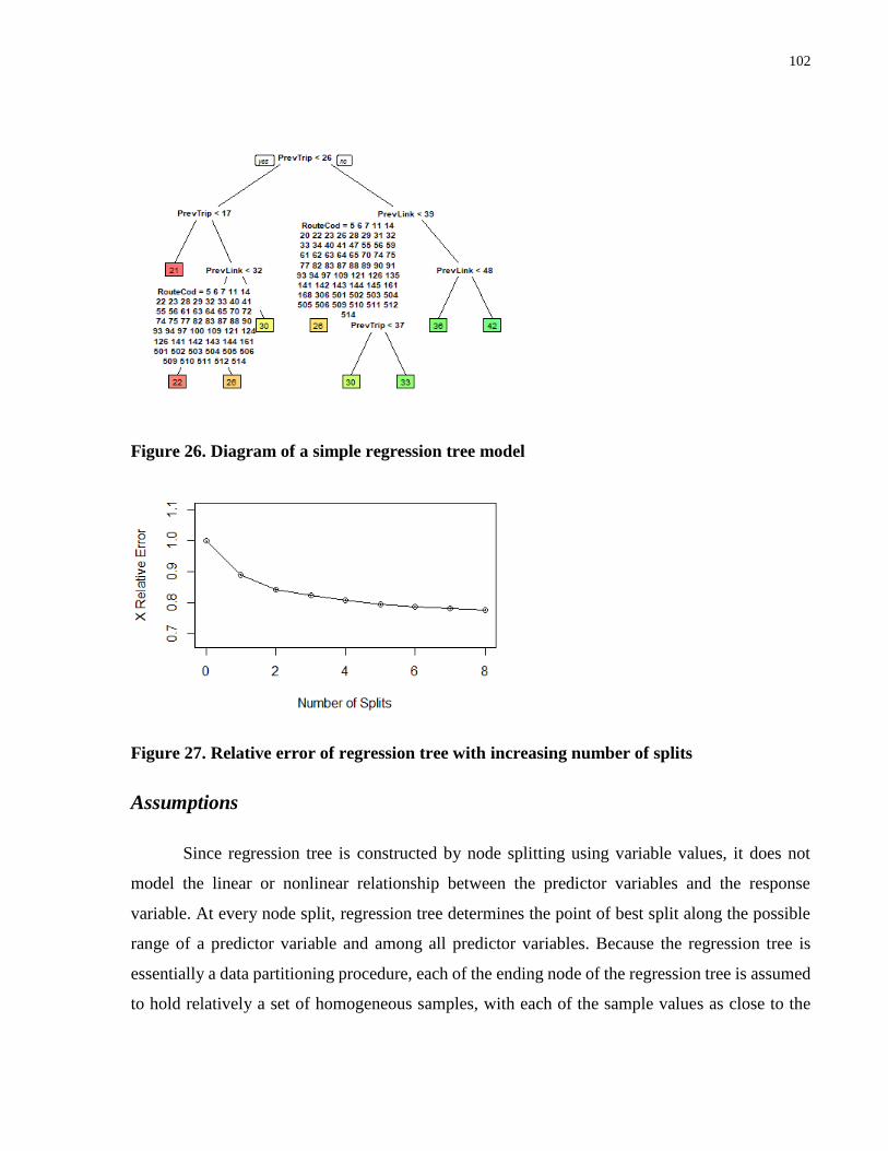
102
Figure 26. Diagram of a simple regression tree model
Figure 27. Relative error of regression tree with increasing number of splits
Assumptions
Since regression tree is constructed by node splitting using variable values, it does not
model the linear or nonlinear relationship between the predictor variables and the response
variable. At every node split, regression tree determines the point of best split along the possible
range of a predictor variable and among all predictor variables. Because the regression tree is
essentially a data partitioning procedure, each of the ending node of the regression tree is assumed
to hold relatively a set of homogeneous samples, with each of the sample values as close to the

103
mean of the node as possible. This leads to the assumption that the samples within each regression
tree node do not hold linear or nonlinear relationships internally.
Another assumption of regression tree stems from the way variables are chosen to when
performing node split. At each node split, a combination of the levels of a categorical variable and
values of a continuous variable will be assessed as a possible split criterion. The variables that are
more important will appear higher up in the nodes of the tree. In addition, the variables with
multiple possible values and levels and are more important may appear more than once,
sometimes, many times on the tree. While important variables are responsible for making multiple
partitions on the tree, less important variables with weaker effects may not appear on the tree nodes
at all. As such, an assumption made by regression tree is that weak effects from less important
variable do not contribute to model fitness. Consequently, outliers and small samples due to rare
occurrences, such as disruptions, have minimal effects on the model.
Applications
The “rpart” package from R was used to estimate regression tree models (Therneau et al.,
2017). A formula, a minimum split size, model complexity and an optional prune complexity are
specified for the regression tree to generate a tree. The formula used is the same across different
methods and consisted of the response variable name with a list of predictor variable names. The
minimum split size has a default of 20 and is a reasonable choice for most modelling applications
(Terry M. Therneau & Elizabeth J. Atkinson, 2017). In addition, the model complexity is the
minimum decrease in impurity before node splitting terminates. It is a stopping criterion for node
splitting during model estimation. Finally, prune complexity is the maximum increase in impurity
the model allows when pruning or removing nodes to limit overfitting.
There are two ways to prevent overfitting for regression trees. The k-fold cross validation
procedure can find the best complexity parameters for the regression tree, without overfitting.
Similar to the way k-fold cross validation was used for support vector machine models in this
thesis, this procedure divides the entire data set into k number of samples and train separate models
on each sample, and evaluate its performance against rest of the (k-1) number of samples. The best

104
model complexity based on this cross-validation procedure is selected. Another way to reduce
overfitting in regression tree is by specifying a pruning complexity parameter. After a tree with
certain complexity parameter (CP), for example, train CP of 0.0015, has been trained, the tree
pruning procedure can be initiated with a prune CP larger than the train CP, such as prune CP of
0.005. The pruned tree is less likely to overfit the data. For this thesis, the k-fold cross validation
procedure was used since it is a more robust means of preventing overfitting and is a very
commonly used method to optimize model parameters.
6.1.3.5 Random Forest
Random forest is a tree ensemble learning method that does not suffer from overfitting. It
is a combination of decision trees, be it regression trees or classification trees, where each tree is
constructed using a random and independent subsample data (Breiman, 2001). Random forest is
an ensemble method because it combines the predictions from many weaker predictors or trees.
This makes the random forest a very flexible machine learning algorithm as it can deal with
nonlinearity, variable dependencies, and heteroscedastic errors. Unlike a single tree, the random
forest can model weaker parameter effects as weaker trees can contain splits of less important
variables with smaller effects. Most importantly, it has been shown that as the number of trees
grown increases, the test or cross-validation error converges to a minimal by the law of large
numbers (see Equation 16) (Breiman, 2001). This means that random forest model does not suffer
from the overfitting problem.
Equation 16. Random forest regression convergence with increasing number of trees
𝐸𝑋,𝑌(𝑌 − 𝑎𝑣𝑘ℎ(𝑋, 𝛩𝑘))2
→ 𝐸𝑋,𝑌(𝑌 − 𝐸Θℎ(𝑋, 𝛩))2
where ℎ(𝑋, Θ𝑘) is the prediction of individual trees,
𝑎𝑣𝑘(ℎ(𝑋, Θ𝑘)) is the average prediction of all individual trees,
𝑌 is the labelled/true value,

105
𝐸Θℎ(𝑋, 𝛩) is the expected prediction from all individual trees (converged result)
Random forest combines results from numerous trees, which enables it to deal with
clustered data and replicate nonlinear relationships. A key requirement of training random forest
is the randomization of subsample draws which aims to achieve low correlations between trees
(Breiman, 2001). This is achieved by performing subsample draws for training individual trees
independently and at random. The ability to grow trees independently allows the random forest to
deal with clusters and nonlinear relationships. Figure 28 shows that a random forest can contain
numerous trees covering a range of variables, giving rise to complex prediction behaviours.
Figure 28. Illustration of a random forest (R. Hänsch & O. Hellwich, 2015)
Assumptions
The model accuracy of any algorithm is dependent on the quality of the data. Data quality
is a particularly important for the random forest. While random forest has been shown to deal with
noise or random errors well, data that are not representative of true relationships can produce
inaccurate models (Louppe, 2014). Besides the need for high quality data, the random forest is a
very flexible and robust nonparametric modelling method that can model any arbitrarily complex
relations, and handle heteroscedasticity, nonlinear relationships, and variable dependencies.
(Louppe, 2014).
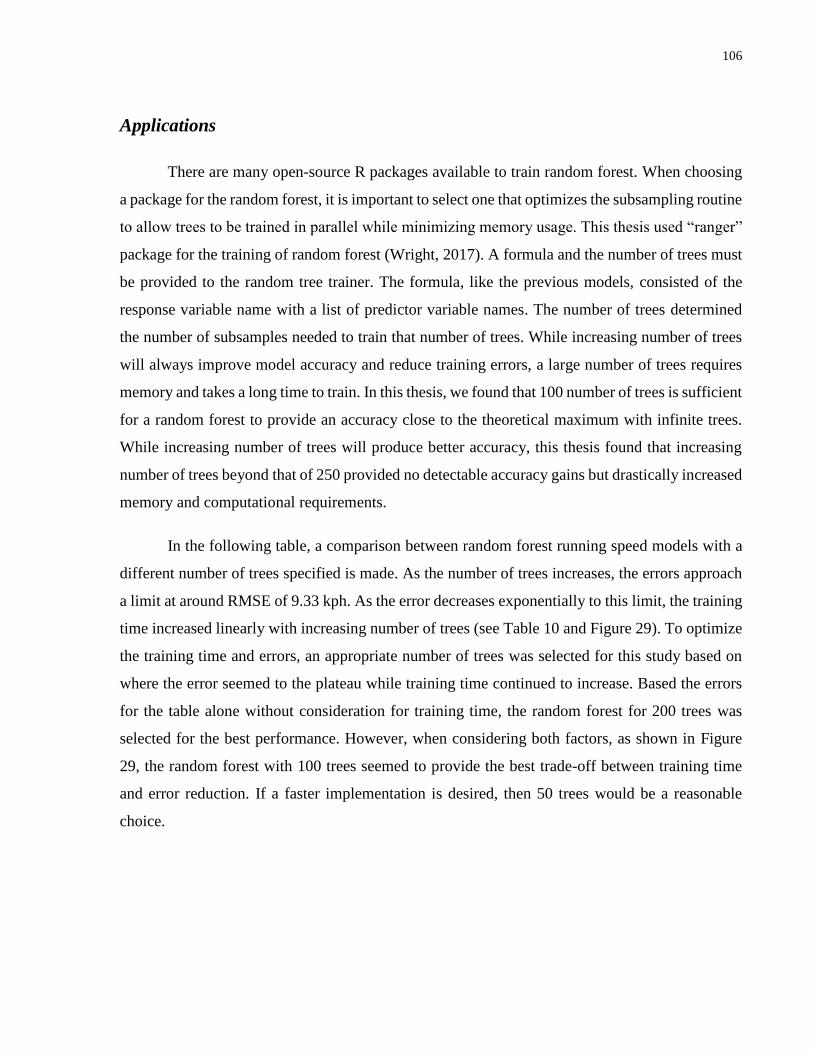
106
Applications
There are many open-source R packages available to train random forest. When choosing
a package for the random forest, it is important to select one that optimizes the subsampling routine
to allow trees to be trained in parallel while minimizing memory usage. This thesis used “ranger”
package for the training of random forest (Wright, 2017). A formula and the number of trees must
be provided to the random tree trainer. The formula, like the previous models, consisted of the
response variable name with a list of predictor variable names. The number of trees determined
the number of subsamples needed to train that number of trees. While increasing number of trees
will always improve model accuracy and reduce training errors, a large number of trees requires
memory and takes a long time to train. In this thesis, we found that 100 number of trees is sufficient
for a random forest to provide an accuracy close to the theoretical maximum with infinite trees.
While increasing number of trees will produce better accuracy, this thesis found that increasing
number of trees beyond that of 250 provided no detectable accuracy gains but drastically increased
memory and computational requirements.
In the following table, a comparison between random forest running speed models with a
different number of trees specified is made. As the number of trees increases, the errors approach
a limit at around RMSE of 9.33 kph. As the error decreases exponentially to this limit, the training
time increased linearly with increasing number of trees (see Table 10 and Figure 29). To optimize
the training time and errors, an appropriate number of trees was selected for this study based on
where the error seemed to the plateau while training time continued to increase. Based the errors
for the table alone without consideration for training time, the random forest for 200 trees was
selected for the best performance. However, when considering both factors, as shown in Figure
29, the random forest with 100 trees seemed to provide the best trade-off between training time
and error reduction. If a faster implementation is desired, then 50 trees would be a reasonable
choice.
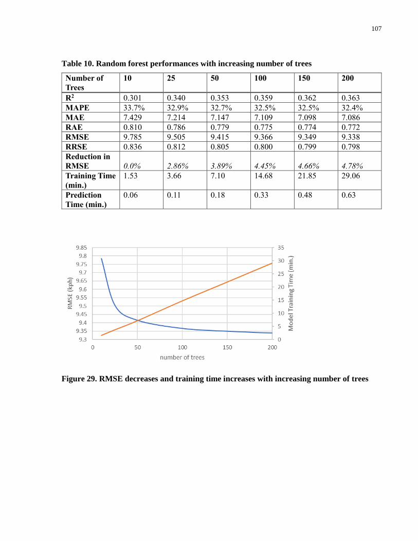
107
Table 10. Random forest performances with increasing number of trees
Number of
Trees
10 25 50 100 150 200
R2 0.301 0.340 0.353 0.359 0.362 0.363
MAPE 33.7% 32.9% 32.7% 32.5% 32.5% 32.4%
MAE 7.429 7.214 7.147 7.109 7.098 7.086
RAE 0.810 0.786 0.779 0.775 0.774 0.772
RMSE 9.785 9.505 9.415 9.366 9.349 9.338
RRSE 0.836 0.812 0.805 0.800 0.799 0.798
Reduction in
RMSE 0.0% 2.86% 3.89% 4.45% 4.66% 4.78%
Training Time
(min.)
1.53 3.66 7.10 14.68 21.85 29.06
Prediction
Time (min.)
0.06 0.11 0.18 0.33 0.48 0.63
Figure 29. RMSE decreases and training time increases with increasing number of trees

108
6.1.4 Model Evaluation
To evaluate the performance of different modelling methods, six error and performance
measurements were computed using equations 1 to 6. They can be used to select a model with the
best prediction performance. While generally a better model provides a lower error and better fit,
each of the error measures a slightly different aspect of the model performance. This section
provides error definitions, their indications, and the possible range of values.
Common notations for calculating model performance measurements are observed values
𝑦𝑖 (y), predicted values �̂�𝑖 (y-hat), and average observed value �̅� (y-bar). Many measurements use
(𝑦𝑖 − �̅�) as base line measurements. A model with all prediction of y-bar is often referred to as the
no relationship horizontal line model, average value model, or default predictor.
6.1.4.1 Coefficient of determination (R2)
The coefficient of determination or R squared is the proportion of the variance explained
by the predictor variable (Allen, 1997). The unexplained error can often be found by computing
the sum of the square of residuals (SSR). Since we know the sum of square, SST, is the difference
between the no relationship horizontal line of �̂�𝑖, the proportion of the unexplained error then is
the quotient between the two, adjusted by degree of freedom. The explained error therefore be one
minus such quotient. The calculation of coefficient of determination is shown in Equation 17. A
typical range of the coefficient of determination is from 0 to 1.
Equation 17. Coefficient of determination
�̅�2 = 1 −SSR dfe⁄
SST dft⁄
where the sum of the square of residual: SSR = ∑ (𝑦𝑖 − �̂�𝑖)2𝑛
𝑖=0
the total sum of the square: 𝑆𝑆𝑇 = ∑ (𝑦𝑖 − �̅�)2𝑛𝑖=0
the degree of freedom: dfe = 𝑛 − 1 dft = 𝑛 − 𝑝 − 1
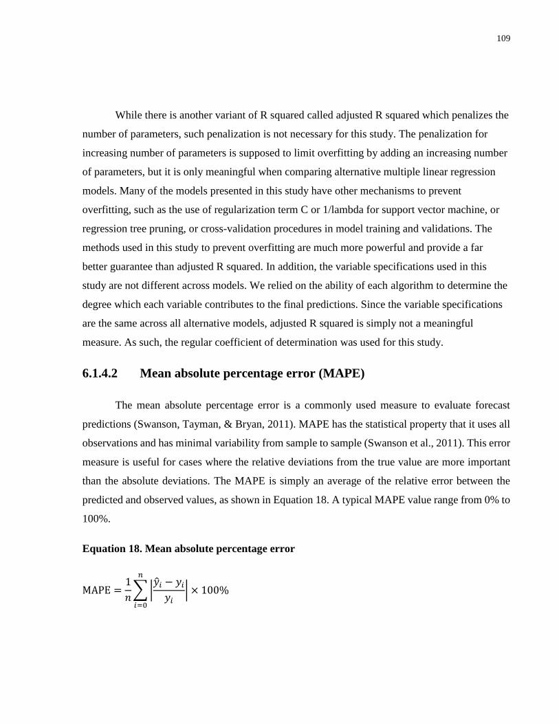
109
While there is another variant of R squared called adjusted R squared which penalizes the
number of parameters, such penalization is not necessary for this study. The penalization for
increasing number of parameters is supposed to limit overfitting by adding an increasing number
of parameters, but it is only meaningful when comparing alternative multiple linear regression
models. Many of the models presented in this study have other mechanisms to prevent
overfitting, such as the use of regularization term C or 1/lambda for support vector machine, or
regression tree pruning, or cross-validation procedures in model training and validations. The
methods used in this study to prevent overfitting are much more powerful and provide a far
better guarantee than adjusted R squared. In addition, the variable specifications used in this
study are not different across models. We relied on the ability of each algorithm to determine the
degree which each variable contributes to the final predictions. Since the variable specifications
are the same across all alternative models, adjusted R squared is simply not a meaningful
measure. As such, the regular coefficient of determination was used for this study.
6.1.4.2 Mean absolute percentage error (MAPE)
The mean absolute percentage error is a commonly used measure to evaluate forecast
predictions (Swanson, Tayman, & Bryan, 2011). MAPE has the statistical property that it uses all
observations and has minimal variability from sample to sample (Swanson et al., 2011). This error
measure is useful for cases where the relative deviations from the true value are more important
than the absolute deviations. The MAPE is simply an average of the relative error between the
predicted and observed values, as shown in Equation 18. A typical MAPE value range from 0% to
100%.
Equation 18. Mean absolute percentage error
MAPE =1
𝑛∑ |
�̂�𝑖 − 𝑦𝑖
𝑦𝑖|
𝑛
𝑖=0
× 100%

110
6.1.4.3 Mean absolute error (MAE)
The mean absolute error considers the unsigned deviation of the predicted value from the
observed value, regardless of the relative sizes of the prediction. This error measure provides an
average of the absolute deviations and is most suitable for uniformly distributed errors (Chai &
Draxler, 2014). Nevertheless, MAE provides average error measure without penalizing the size of
the error, thus indicate an average expected error without exaggerating the effect of outliers
(Witten, Frank, & Hall, 2011). Calculation of MAE is shown in Equation 19. MAE values can
range from 0 to infinity.
Equation 19. Mean absolute error
MAE =1
𝑛∑|�̂�𝑖 − 𝑦𝑖|
𝑛
𝑖=0
6.1.4.4 Relative absolute error (RAE)
The relative absolute error is the absolute error normalized by the residual from the simple
average value predictor (Witten et al., 2011). The benefit of relative error is that it makes a
comparison between the current model and the simple horizontal line model (see Equation 20).
The lower the RAE, the better the model is compared to the simple horizontal line model. The
typical value of RAE ranges from 0 to 1, with 0 being a perfect model that explains all errors and
1 being a model equivalent to the average value model. It is possible for models to perform worse
than the average value model.
Equation 20. Relative absolute error
RAE =∑ |�̂�𝑖 − 𝑦𝑖|
𝑛𝑖=0
∑ |𝑦𝑖 − �̅�|𝑛𝑖=0

111
6.1.4.5 Root mean square error (RMSE)
The root mean square error is one of the most commonly used error measurements in
comparing model performance (see Equation 21) (Witten et al., 2011). The underlying assumption
of RMSE is that the errors are unbiased and are normally distributed (Chai & Draxler, 2014). Since
RMSE assumes normally distributed errors, it penalizes large errors at a greater extent than small
errors. It is generally considered a better representation of normally distributed errors (Chai &
Draxler, 2014). However, RMSE may overestimate error values if the observed values are not
strictly normal. A typical value of RMSE can range from 0 to infinity.
Equation 21. Root mean square error
RMSE = √1
𝑛∑(𝑦�̂� − 𝑦𝑖)2
𝑛
𝑖=0
6.1.4.6 Root relative square error (RRSE)
The root relative square error takes the RMSE and normalize it to the default predictor (see
Equation 22) (Witten et al., 2011). It combines the advantage of accurately representing outliers
and comparing the model errors to the no relationship horizontal line model. Lower RRSE
indicates a model that reduces outlier errors and total errors much better than the average value
model. A typical value of RRSE ranges from 0 to 1, but infinite RRSE is possible if the model
performs significantly worse than the default predictor.
Equation 22. Root relative square error
RRSE = √∑ (�̂�𝑖 − 𝑦𝑖)2𝑛
𝑖=0
∑ (𝑦𝑖 − �̅�)2𝑛𝑖=0
112
6.1.4.7 Training and Prediction Time
The training and prediction time can differ greatly between machine learning algorithms
due to differing mathematical and software implementations. In this thesis, the time required to
train and test a machine learning model was recorded for each model as an additional model
selection criteria. The training time refers to the duration it takes for a machine learning package
to use the input training data and model specification to compute and return a trained model object.
On the other hand, the prediction time refers to the duration it takes for the machine learning
package to use the input test data and trained model object to return a list of predictions, previously
referred to as �̂�𝑖, y-hat. In general, the prediction time is lower than training time. The training and
prediction times were reported in minutes.
6.2 Dwell Time Model
Previous studies have demonstrated that transit dwell times follow a lognormal distribution
(Li, Duan, & Yang, 2012). The characteristics of lognormal distribution are consistent with many
of the properties of dwell time. Firstly, dwell times can only be positive. Secondly, dwell times is
a continuous variable. Finally, dwell times are often right skewed with infrequent large dwell times
and frequent small to median dwell times.
The lognormal distribution parameters of dwell times were estimated and evaluated. The
training data were loaded and all the dwell time observations were organized into stops. Then, a
lognormal distribution of dwell time was estimated for each stop. Finally, the dwell time
predictions across all stops in the network were compared against test data to evaluate the fitness
of the lognormal distribution models.
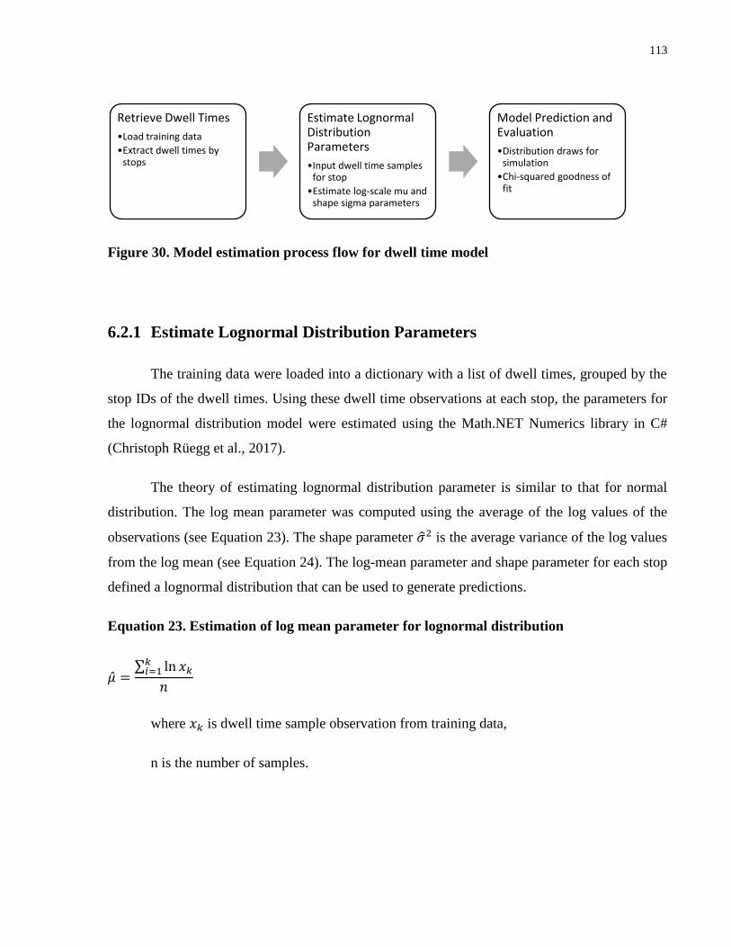
113
Figure 30. Model estimation process flow for dwell time model
6.2.1 Estimate Lognormal Distribution Parameters
The training data were loaded into a dictionary with a list of dwell times, grouped by the
stop IDs of the dwell times. Using these dwell time observations at each stop, the parameters for
the lognormal distribution model were estimated using the Math.NET Numerics library in C#
(Christoph Rüegg et al., 2017).
The theory of estimating lognormal distribution parameter is similar to that for normal
distribution. The log mean parameter was computed using the average of the log values of the
observations (see Equation 23). The shape parameter �̂�2 is the average variance of the log values
from the log mean (see Equation 24). The log-mean parameter and shape parameter for each stop
defined a lognormal distribution that can be used to generate predictions.
Equation 23. Estimation of log mean parameter for lognormal distribution
�̂� =∑ ln 𝑥𝑘
𝑘𝑖=1
𝑛
where 𝑥𝑘 is dwell time sample observation from training data,
n is the number of samples.
Retrieve Dwell Times
•Load training data
•Extract dwell times by stops
Estimate Lognormal Distribution Parameters
•Input dwell time samples for stop
•Estimate log-scale mu and shape sigma parameters
Model Prediction and Evaluation
•Distribution draws for simulation
•Chi-squared goodness of fit
114
Equation 24. Estimation of shape parameter for lognormal distribution
�̂�2 =∑ (ln 𝑥𝑘 − �̂�)2𝑘
𝑖=1
𝑛
where 𝑥𝑘 is dwell time sample observation from training data,
n is the number of samples,
�̂� is the log mean.
6.2.2 Dwell Time Model Evaluations
The dwell time distribution for each stop was used to generate the dwell time predictions
during simulation. The chi-square test was used to assess the goodness of fit of the predicted dwell
times. Since the dwell times at each stop were estimated based on AVL data points, the resolution
of dwell times was 20 seconds. This means that a bin size of at least 20 seconds must be used to
conduct the chi-square test. The chi-square test statistic was then computed with the predicted
dwell time frequency (𝑃𝑖) and observed dwell time frequency (𝑂𝑖), using Equation 25. The null
hypothesis that “the predicted dwell times follow the distribution of the observed dwell times” was
evaluated using the chi-square test statistics. If the critical chi-square value is less than the
computed chi-square value, the null hypothesis would be rejected.
Equation 25. Chi-squared test statistics
𝜒2 = ∑ (𝑃𝑖 − 𝑂𝑖)2 𝑂𝑖⁄
where 𝑃𝑖 is the predicted dwell time frequency,
𝑂𝑖 is observed dwell time frequency

115
6.3 Summary
This chapter presented the procedure this thesis used to perform model estimation for
running speed and dwell time models. After retrieving processed data and specifying model
parameters, this thesis trained five different machine learning models for running speed: multiple
linear regression, support vector machine, linear mixed effect model, regression trees, and random
forest. The theory, assumptions, and applications of each model type were discussed in detailed.
Finally, six different model performance and error measurements were calculated to
comprehensively compare the ability of these models to capture errors under various assumptions.
The running speed model with the best fit and performance was selected to represent the running
speeds for large-scale transit simulations. Similarly, lognormal dwell time models for every stop
across the network were estimated using dwell times from training data. The goodness of fit of the
dwell time models was evaluated using the chi-square test. The estimated models for running
speeds and dwell times were used to generate simulated transit trips.
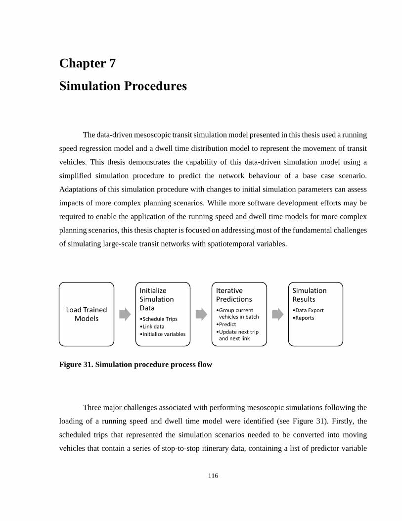
116
Chapter 7
Simulation Procedures
The data-driven mesoscopic transit simulation model presented in this thesis used a running
speed regression model and a dwell time distribution model to represent the movement of transit
vehicles. This thesis demonstrates the capability of this data-driven simulation model using a
simplified simulation procedure to predict the network behaviour of a base case scenario.
Adaptations of this simulation procedure with changes to initial simulation parameters can assess
impacts of more complex planning scenarios. While more software development efforts may be
required to enable the application of the running speed and dwell time models for more complex
planning scenarios, this thesis chapter is focused on addressing most of the fundamental challenges
of simulating large-scale transit networks with spatiotemporal variables.
Figure 31. Simulation procedure process flow
Three major challenges associated with performing mesoscopic simulations following the
loading of a running speed and dwell time model were identified (see Figure 31). Firstly, the
scheduled trips that represented the simulation scenarios needed to be converted into moving
vehicles that contain a series of stop-to-stop itinerary data, containing a list of predictor variable
Load Trained Models
Initialize Simulation Data
•Schedule Trips
•Link data
•Initialize variables
Iterative Predictions
•Group current vehicles in batch
•Predict
•Update next trip and next link
Simulation Results
•Data Export
•Reports
117
values identical to link data. Another challenge was to perform as many predictions in parallel
while updating the vehicle itinerary data in proper order. Many of the predictor variables were
spatiotemporal in nature, so they needed to be updated in order of space and time as well. Some
of the examples of these predictor variables were previous link speed, previous trip speed,
headway, and delay. To update the vehicle itinerary data, this thesis grouped vehicles into batches,
perform predictions, then updated the next link’s and next trip’s vehicle itinerary data. Finally,
after simulation, an important challenge was to extract all the vehicle itinerary information to
enable analysis and generation of reports. The last section of this chapter will represent the
reporting functions used to generate time-distance diagrams, route speed reports, and stop delay
reports.
7.1 Load Trained Models
The running speed models presented in this thesis were trained in an R workbench. Since
the simulation procedure was written in C#, we needed to call R scripts from the C# environment.
R.Net is an in-process interoperability bridge to R from the Dot-Net languages that are capable of
establishing R instances inside of Dot-Net framework (Jean-Michel Perraud, 2015). R.Net allows
one to initiate an R workbench instance from C# and perform any given R function. As such, the
training and loading of running speed model were done in an R workbench instance inside C#.
Before simulation begins, the procedure loads the workbench with the trained running speed model
into the R workbench in memory.
In contrast, the dwell time models were trained in the native C# environment. As a result,
there were no interoperability considerations. The dwell time models were loaded onto memory
before the start of the model simulation. The models were stored in a dictionary indexed by their
stop code. During simulation run time, the dwell time model for a specific stop was used to draw
a random dwell time from the estimated lognormal distribution.
118
7.2 Initialize Simulation Data
After loading the trained models, the simulation data representing vehicles needed to be
prepared for model predictions. The simulation data object contained possible movements of
vehicles from one stop to another. The simulation data object was a dictionary object containing a
list of vehicle movements indexed by the GTFS trip ID. The initialization step constructed the
simulation data object using the GTFS schedule trips and initialized predictor variable values
needed for speed prediction.
To initialize the vehicle movement data, a list of appropriate GTFS trips within the study
period was obtained from the GTFS trip data. The GTFS trip data were first filtered by their service
ID to ensure only the weekday or weekend were included. Then, they were filtered by the trip’s
start and end times. The start time of the trip was required to be before the end time of the study
period, and the end time of the trip must be after the start time of the study period. This ensured
that all of the possible vehicles travelling within the study period were captured, and the vehicles
travelling entirely out the study period were not modelled. After a list of GTFS trips within the
study period was determined, all the vehicle movements from stop to stop for each trip were
generated and stored in a list. The list was sorted by time.
Before predictions on the response variable, running speed and dwell time, could be carried
out, the values of all the predictor variables needed to be specified. The initialization of simulation
data assigns the following predictor variables: stop sequence, start stop ID and code, end stop ID
and code, time of day, route code, link name, start stop scheduled arrival time, end stop scheduled
arrival time, schedule headway, total precipitation, incident occurrence, link distance, is streetcar,
is separated ROW, number of vehicle left, number of vehicle right, number of vehicle through
movements, number of intersections with TSP equipped, number of pedestrian crossings, average
vehicle volume along the transit link, average pedestrian volume along the transit link, is start stop
near sided and is end stop far sided.
The listed predictor variables correspond to the variables previously discussed for model
estimation of running speed models. This part of the procedure populated the variables in two
119
ways. The simplest way is through referencing stop and schedule information in GTFS. For
instance, stop sequence, start stop ID, end stop ID, time of day, route code, link name, start stop
scheduled arrival time, end stop scheduled arrival time, and schedule headway were variables that
were directly obtained from schedule information contained in the GTFS tables, accessible to
model simulation. The remaining variables, total precipitation, incident occurrence, link distance,
is streetcar, is separated ROW, number of vehicle left, number of vehicle right, number of vehicle
through movements, number of intersections with TSP equipped, number of pedestrian crossings,
average vehicle volume along the transit link, average pedestrian volume along the transit link, is
start stop near sided and is end stop far sided, were obtainable using the processed data from AVL,
intersection, weather, and road restriction data. Therefore, a test day data was required for
simulation. It is important that only a few of the variables presented were day dependent: total
precipitation and incident occurrence. Modification of these variables at selected links would be a
viable way to test different scenarios across the network such as heavy rain and multiple roadway
incidents.
All the vehicle movement data were initialized using information from GTFS schedules
and the day of test data (see left side of Figure 32). These vehicle movement data were finally
placed into the simulation data object, Sim_ModelData_ByGtfsTripID, where the ordered list of
vehicle movements for each GTFS trip was indexed by the GTFS trip for easy retrieval.
7.3 Iterative Predictions
The simulation data object itself contained all the possible movements of vehicles from
one stop to another for a GTFS trip; however, there were still a number of transit operational
variables that needed to be obtained before predictions could be obtained: previous link speed,
previous trip speed, terminal stop delay, stop delay, simulated headway, headway ratio. The
iterative prediction algorithm updated these missing variables as predictions were carried out in an
iterative manner (see right side of Figure 32). The iterative procedure ran until all of the vehicle
movements (samples) were predicted. The iterative prediction algorithm performed three major

120
steps: creating sample batch ready for prediction, performing prediction on the batch, and variable
updating for the next round of predictions. Performing predictions and updates in batches allowed
model simulations to be carried out in a computationally efficient manner.
Figure 32. Flowchart of model simulation procedure
Vehicle movements could become ready for prediction in two ways. If the vehicle
movement occurred at the first stop of the first trip of a vehicle block, then the movement was
always ready and would be predicted in the first batch of prediction. These first stop of the block
vehicle movements used default values for transit operational variables: previous link speed = 0,
previous trip speed = 0, terminal stop delay = 0, stop delay = 0, simulated headway = schedule
headway, headway ratio = 1. For all other vehicle movements, they become ready when all of the
above 7 variables were updated during the variable update step. The samples that were ready for
prediction received running speed and dwell time predictions.

121
The prediction step involved the algorithm collecting all of the samples and converting
them into a format that could be used to create predictions. Batched sample predictions reduced
compute time since the model prediction method in R was optimized for parallelized computations
with large sample data batches. The sample batch was first converted into an R.Net DataFrame
table object in C#, then passed to the R workbench. The DataFrame table, now residing inside the
R workbench, was used to generate running speed predictions. The running speed predictions were
returned to C# as an array of Numerics object. These running speed predictions were used to update
the current samples’ running speed values. Dwell time predictions for the current sample were
obtained by performing a random distribution draw using the dwell time models for the start stop.
Using running speed and dwell time predictions, the departure time at start stop and arrival time
at end stop could be computed for these samples as well. At the end of the prediction step, the
samples with the predicted running speed and dwell time were updated to the
Sim_ModelPredOutput_ByGtfsTripID object that contained all of the predicted vehicle
movements. At the same time, the previous GTFS trip ID, GTFS trip ID, block ID, block sequence
were updated as well. These variables, along with running speed and dwell time were used to
update variables for the next steps of prediction.
The variable update was an important step to ensure vehicle movements were consistent
and connected. The variable update was performed on every remaining sample where there are
still missing variables. The previous link speed and arrival time at start stop were updated using
the speed prediction and arrival at end stop from the previous link of the same trip. The previous
trip speed was updated using the speed prediction from the previous trip on the same link. Using
the arrival times of the current trip and previous trip on the same link, the stop headway and
headway ratio were computed. Finally, the stop delay and terminal stop delay were computed
based on the difference between scheduled arrival time and simulated arrival time at the start stop.
The variable update step kept the simulation consistent and allow the next sample batch to be
formed for prediction.
As predictions were carrying out for every sample, the samples with completed predictions
were stored in a simulated trip object, Sim_ModelPredOutput_ByGtfsTripID. This object

122
contained the records of all the simulated vehicle movements of the GTFS trips. Using the
procedure for iterative predictions with three major steps, a network of simulated vehicle
movements was obtained using the GTFS schedule trips.
7.4 Simulation Result Outputs
The simulated trip object obtained from the iterative prediction step was exported into a
binary data object for debugging and software development use. In addition, the simulated trip
object was converted into comma separated value (CSV) format for general analysis. This section
describes the format and use of these outputs of the simulation result.
7.4.1 Binary Simulation Data
The binary simulation data file, “CSharp_Sim_ModelDataPred.bin,” was a serialized
binary object of Sim_ModelPredOutput_ByGtfsTripID. This binary file was a dictionary object
containing lists of vehicle movements indexed by GTFS trip ID. One use of the binary file is to
allow the simulated vehicle movements to be saved and retrieved for report generation (discussed
in the next section). This way, simulation for a scenario can be saved and retrieved later for analysis
and reporting. Another use for the binary data file is for integration with Nexus. The vehicle
movements can be read by Nexus coordinator classes to connect the simulated surface transit
vehicle movements with the pedestrian and station models used by Nexus. A binary file can
efficiently save simulation result for future use.
7.4.2 Summary Data File
In addition to saving the simulation to binary, the simulation procedure also wrote
summary data in CSV format. Unlike binary files, which are not human readable, CSV files could
be used to analyse the fields of vehicle movements. Since for every simulated vehicle movement,
there was a scheduled vehicle movement, a simulated results CSV file can be exported containing
these movements with fields such as simulated arrival time at start stop, scheduled arrival time at
start stop, etc. In contrast, there was not a one to one correspondence between the observed vehicle

123
movements from processed AVL data; therefore, a separate observed results CSV file was
generated. The observed results CSV file contained all the data fields of the observed results. These
CSV files were exported from the final simulation data and test data for simulation; they were used
for general analysis and reporting.
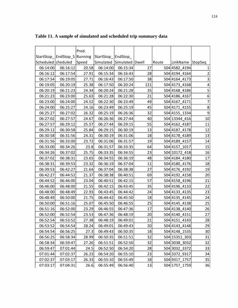
124
Table 11. A sample of simulated and scheduled trip summary data
StartStop_
Scheduled
EndStop_S
cheduled
Pred.
Running
Speed
StartStop_
Simulated
EndStop_
Simulated Dwell Route LinkName StopSeq
06:14:00 06:16:12 20.58 06:14:00 06:15:34 27 504 4582_4194 1
06:16:12 06:17:54 27.91 06:15:34 06:16:43 28 504 4194_4164 2
06:17:54 06:19:05 27.71 06:16:43 06:17:50 38 504 4164_4173 3
06:19:05 06:20:19 25.38 06:17:50 06:20:24 121 504 4173_4168 4
06:20:19 06:21:23 24.34 06:20:24 06:21:28 35 504 4168_4186 5
06:21:23 06:23:00 25.63 06:21:28 06:22:30 21 504 4186_4167 6
06:23:00 06:24:00 24.52 06:22:30 06:23:49 49 504 4167_4171 7
06:24:00 06:25:27 24.16 06:23:49 06:25:19 45 504 4171_4155 8
06:25:27 06:27:02 26.32 06:25:19 06:26:36 32 504 4155_13344 9
06:27:02 06:27:57 24.67 06:26:36 06:27:44 40 504 13344_4162 10
06:27:57 06:29:12 25.57 06:27:44 06:29:15 55 504 4162_4187 11
06:29:12 06:30:58 25.84 06:29:15 06:30:19 13 504 4187_4178 12
06:30:58 06:31:56 24.31 06:30:19 06:31:06 18 504 4178_4189 13
06:31:56 06:33:00 23.72 06:31:06 06:31:57 19 504 4189_4157 14
06:33:00 06:34:26 23.8 06:31:57 06:33:35 64 504 4157_10172 15
06:34:26 06:37:02 25.75 06:33:35 06:34:55 23 504 10172_4184 16
06:37:02 06:38:31 23.65 06:34:55 06:36:19 48 504 4184_4180 17
06:38:31 06:39:53 23.32 06:36:19 06:37:04 11 504 4180_4176 18
06:39:53 06:42:27 21.64 06:37:04 06:38:38 27 504 4176_4192 19
06:42:27 06:44:52 21.37 06:38:38 06:40:51 69 504 4192_4158 20
06:44:52 06:46:00 23.04 06:40:51 06:42:15 57 504 4158_4196 21
06:46:00 06:48:00 21.55 06:42:15 06:43:45 35 504 4196_4133 22
06:48:00 06:48:49 22.93 06:43:45 06:44:42 24 504 4133_4135 23
06:48:49 06:50:00 21.75 06:44:42 06:45:50 18 504 4135_4145 24
06:50:00 06:51:16 25.07 06:45:50 06:46:55 25 504 4145_4138 25
06:51:16 06:52:00 23.29 06:46:55 06:47:36 17 504 4138_4140 26
06:52:00 06:52:54 23.53 06:47:36 06:48:19 20 504 4140_4151 27
06:52:54 06:53:52 27.38 06:48:19 06:49:01 21 504 4151_4143 28
06:53:52 06:54:54 28.24 06:49:01 06:49:43 20 504 4143_4148 29
06:54:54 06:56:25 27.3 06:49:43 06:50:35 18 504 4148_15351 30
06:56:25 06:58:34 28.99 06:50:35 06:51:51 32 504 15351_3038 31
06:58:34 06:59:47 27.26 06:51:51 06:52:50 32 504 3038_3032 32
06:59:47 07:01:44 24.5 06:52:50 06:54:20 28 504 3032_3372 33
07:01:44 07:02:37 26.23 06:54:20 06:55:10 23 504 3372_9317 34
07:02:37 07:03:17 26.33 06:55:10 06:55:49 18 504 9317_1757 35
07:03:17 07:04:31 26.6 06:55:49 06:56:40 13 504 1757_1759 36
07:04:31 07:05:28 30.68 06:56:40 06:57:26 20 504 1759_1766 37
07:05:28 07:06:45 31.22 06:57:26 06:58:19 20 504 1766_1761 38
07:06:45 07:08:06 31.97 06:58:19 06:59:52 58 504 1761_1768 39
07:08:06 07:09:12 29.72 06:59:52 07:01:00 38 504 1768_1755 40
07:09:12 07:10:00 23.1 07:01:00 07:01:57 31 504 1755_14639 41

125
Table 12. A sample of observed trip summary data from test data set
StartStop_
Observed
EndStop_
Observed
Running
Speed Dwell
Route
Code Link Name StopSeq
06:14:06 06:18:48 7.27 0 504 11155_4194 1
06:18:48 06:19:23 32.66 0 504 4194_4164 2
06:19:23 06:20:19 14.25 0 504 4164_4173 3
06:20:19 06:21:03 18.85 0 504 4173_4168 4
06:21:03 06:21:36 21.68 0 504 4168_4186 5
06:21:36 06:22:28 20.14 0 504 4186_4167 6
06:22:28 06:23:21 14.17 0 504 4167_4171 7
06:23:21 06:24:37 14.22 0 504 4171_4155 8
06:24:37 06:26:28 13.28 22 504 4155_13344 9
06:26:28 06:27:00 21.24 0 504 13344_4162 10
06:27:00 06:28:03 21.73 20 504 4162_4187 11
06:28:03 06:29:24 19.8 15 504 4187_4178 12
06:29:24 06:30:14 14.43 0 504 4178_4189 13
06:30:14 06:31:00 16.04 0 504 4189_4157 14
06:31:00 06:31:58 14.04 0 504 4157_10172 15
06:31:58 06:33:42 17.88 21 504 10172_4184 16
06:33:42 06:34:51 12.23 0 504 4184_4180 17
06:34:51 06:35:53 18.09 19 504 4180_4176 18
06:35:53 06:37:50 12.48 0 504 4176_4192 19
06:37:50 06:40:50 16.79 98 504 4192_4158 20
06:40:50 06:41:47 16.74 20 504 4158_4196 21
06:41:47 06:43:52 9.37 0 504 4196_4133 22
06:43:52 06:44:31 19.5 0 504 4133_4135 23
06:44:31 06:45:38 23.41 20 504 4135_4145 24
06:45:38 06:46:53 13.27 0 504 4145_4138 25
06:46:53 06:47:31 14.85 0 504 4138_4140 26
06:47:31 06:48:29 9.27 0 504 4140_4151 27
06:48:29 06:49:04 16.46 0 504 4151_4143 28
06:49:04 06:49:30 23.9 0 504 4143_4148 29
06:49:30 06:51:12 14.42 39 504 4148_15351 30
06:51:12 06:52:55 12.52 0 504 15351_3038 31
06:52:55 06:53:30 20.83 0 504 3038_3032 32
06:53:30 06:55:10 19.18 21 504 3032_3372 33
06:55:10 06:58:26 12.83 140 504 3372_9317 34
06:58:26 06:58:50 23.02 0 504 9317_1757 35
06:58:50 07:00:19 14.87 21 504 1757_1759 36
07:00:19 07:00:54 22.45 0 504 1759_1766 37
07:00:54 07:01:39 23.25 0 504 1766_1761 38
07:01:39 07:02:28 22.69 0 504 1761_1768 39
07:02:28 07:03:10 21.47 0 504 1768_1755 40
07:03:10 07:05:09 12.34 64 504 1755_14639 41

126
7.5 Analytic Reports
While the summary data contained the complete vehicle movement data, analysing the
summary data on the vehicle movements of the entire network, by stop or by route, can be very
time-consuming. This thesis presents ways to automate the analysis and reporting of vehicle
movement data. The report generation methods in this thesis used OfficeOpenXML tools from the
EPPlus package as well as plotting packages in R via R.Net from C#. This thesis demonstrated
three types of analytics reports for transit vehicle movements: time distance diagrams for vehicle
trajectory analysis, route speed histograms for route-level analysis, and stop delay distributions for
stop-level analysis.
7.5.1 Time Distance Diagrams
The time distance diagram is commonly used to examine the vehicle trajectories of transit
vehicles along a route (see Figure 33). The y axis of the diagram is the distance from the start of a
route and the x axis of the diagram is time. In order to generate this type of diagram properly, the
vehicle movement data of different trips needed to be grouped into their appropriate route and
direction. After the trips were grouped by their routes, the reports were generated using the stop
arrival and departure times for scheduled trips, simulated trips and observed trips. The graph data
along with the time distance diagram were saved as a Microsoft Excel file for that route and
direction. This procedure was repeated for each route and direction to generate time and distance
diagrams for all trips.
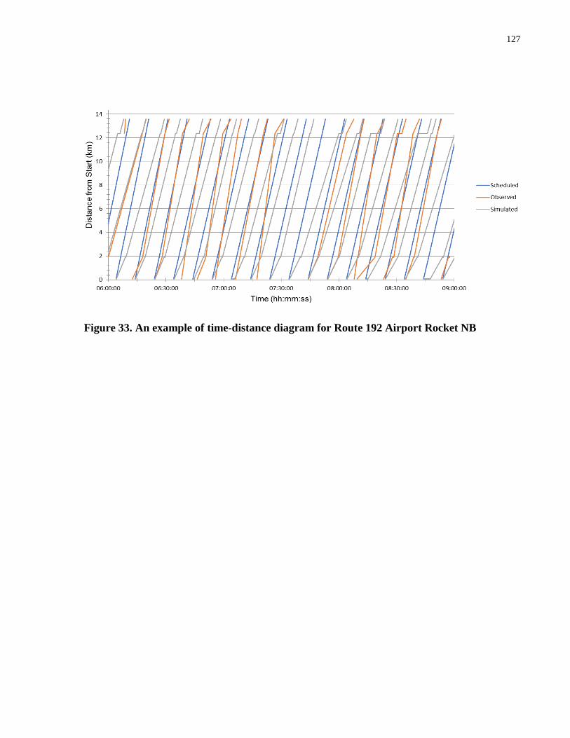
127
Figure 33. An example of time-distance diagram for Route 192 Airport Rocket NB
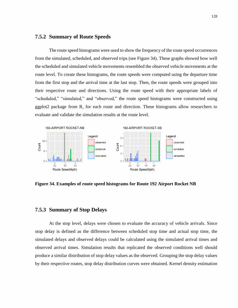
128
7.5.2 Summary of Route Speeds
The route speed histograms were used to show the frequency of the route speed occurrences
from the simulated, scheduled, and observed trips (see Figure 34). These graphs showed how well
the scheduled and simulated vehicle movements resembled the observed vehicle movements at the
route level. To create these histograms, the route speeds were computed using the departure time
from the first stop and the arrival time at the last stop. Then, the route speeds were grouped into
their respective route and directions. Using the route speed with their appropriate labels of
“scheduled,” “simulated,” and “observed,” the route speed histograms were constructed using
ggplot2 package from R, for each route and direction. These histograms allow researchers to
evaluate and validate the simulation results at the route level.
Figure 34. Examples of route speed histograms for Route 192 Airport Rocket NB
7.5.3 Summary of Stop Delays
At the stop level, delays were chosen to evaluate the accuracy of vehicle arrivals. Since
stop delay is defined as the difference between scheduled stop time and actual stop time, the
simulated delays and observed delays could be calculated using the simulated arrival times and
observed arrival times. Simulation results that replicated the observed conditions well should
produce a similar distribution of stop delay values as the observed. Grouping the stop delay values
by their respective routes, stop delay distribution curves were obtained. Kernel density estimation

129
method was applied to the stop delay data using the ggplot2 package from R to produce probability
density curves for simulated and observed stop delays.
Figure 35. Examples of stop delay distribution curve
7.6 Summary
The simulation procedures used by this thesis resolved major challenges associated with
large-scale transit simulations. To enable efficient model loading, the challenges associated with
working across programming platforms (R and C#) were resolved by using R.Net to host R
workbench instance within C#. Simulation data was initialized to establish a base case simulation
scenario based on GTFS schedule trips. Then, running speed and dwell time predictions were
generated in a computationally efficient manner using an iterative prediction procedure with data
sample batching. Using these predictions, a network of transit trips was simulated and the results
of the simulation were exported for analysis. In addition, this thesis presented an innovative
method to automate the generations of time distance diagrams, route speed histograms, and stop
delay distribution curves to evaluate and validate the simulation models. Finally, the simulated
surface transit model enabled analysis of network behaviours and allowed for the integration of
multimodal transit models.
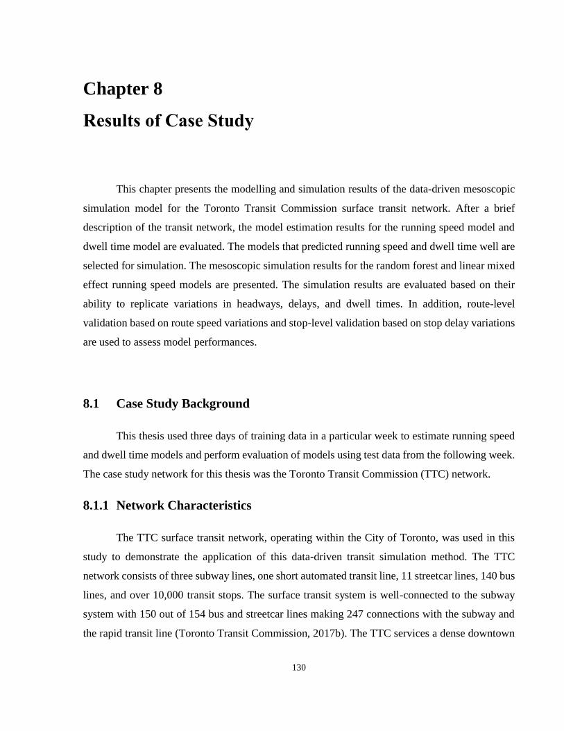
130
Chapter 8
Results of Case Study
This chapter presents the modelling and simulation results of the data-driven mesoscopic
simulation model for the Toronto Transit Commission surface transit network. After a brief
description of the transit network, the model estimation results for the running speed model and
dwell time model are evaluated. The models that predicted running speed and dwell time well are
selected for simulation. The mesoscopic simulation results for the random forest and linear mixed
effect running speed models are presented. The simulation results are evaluated based on their
ability to replicate variations in headways, delays, and dwell times. In addition, route-level
validation based on route speed variations and stop-level validation based on stop delay variations
are used to assess model performances.
8.1 Case Study Background
This thesis used three days of training data in a particular week to estimate running speed
and dwell time models and perform evaluation of models using test data from the following week.
The case study network for this thesis was the Toronto Transit Commission (TTC) network.
8.1.1 Network Characteristics
The TTC surface transit network, operating within the City of Toronto, was used in this
study to demonstrate the application of this data-driven transit simulation method. The TTC
network consists of three subway lines, one short automated transit line, 11 streetcar lines, 140 bus
lines, and over 10,000 transit stops. The surface transit system is well-connected to the subway
system with 150 out of 154 bus and streetcar lines making 247 connections with the subway and
the rapid transit line (Toronto Transit Commission, 2017b). The TTC services a dense downtown

131
area of Toronto where almost all of its streetcar lines run through with major connections at every
subway station (see Figure 36).
Figure 36. The Toronto Transit Commission downtown network map (Toronto Transit
Commission, 2017c)
8.1.2 Study Period
The study period selected for model training was from February 28, 2017 to March 2, 2017.
A large-scale weekday morning peak-period (6:00 to 9:00) running speed and dwell time model
was developed using the training data for this study period. To perform a statistical analysis on the
running speed model, test data from March 7, 2017 to March 9, 2017 were used. To validate the
running speed and dwell time models at the stop and route level of the network, schedule trips
132
from a typical weekday with reference test data from March 8, 2017 were used to simulate transit
trips. Leveraging the availability of open data and the capability of machine learning algorithms,
this case study demonstrates a data-driven method for large-scale transit simulation modelling.
8.2 Summary of Data
The training and test data were necessary for the estimation and evaluation of models. This
thesis used five different data sets within the defined study periods: General Transit Feed
Specification (GTFS), Automatic Vehicle Location (AVL), road restriction, weather, and traffic
intersection data. A description, the type of link variables, as well as the quantity of each type of
data are detailed in Table 13.
A transit schedule contained a set of weekday, weekend, and holiday trips with relevant
stop and route information. Using the schedule information in the GTFS data set for the TTC, the
schedule arrival times, schedule headway, route number, and link distances were obtained for
every vehicle trip. For a typical AM-peak weekday schedule from 6 AM to 9AM, there were 8304
scheduled transit trips. These transit trips were used extensively from data processing to model
evaluation.
The AVL data set for TTC contained the actual vehicle trajectories for the entire network.
Many of the link variables based on the observed vehicle position were obtained, such as the arrival
times, dwell times, running speeds, delays, and headways. Due to operational conditions, the TTC
may short-turn trips or dispatch additional surface transit service. This likely explains the
differences in the number of trips between the AVL data and the GTFS data. The number of AVL
trips ranged from 8350 to 8428 for the set of training and test data used.
The reported road events contained in the road restriction data covered the entire City of
Toronto. This thesis used the locations of road restrictions to determine if there were incident
occurrences on a particular transit link at a particular time. The incident occurrences associated
with each link were recorded to explore the effect of road closures and incidents on transit running
133
speeds. There were 734 road restriction events during the training data period and 766 road
restriction events during the test data period.
In addition to road events, the total precipitation of the transit link within a particular period
were determined based on proximity of the weather stations to the link. Using the various weather
station data from Toronto, 72 weather records were collected each day. These weather records
were used to determine the total precipitation on a transit link for a given time.
Finally, the traffic intersection data consist information from a list of all the signalized
intersections, pedestrian crossings, and flashing beacons in the City of Toronto. Using the
intersection data and the geometry of the scheduled routes from the GTFS data, various transit link
characteristics were determined. Some examples of transit link characteristics were number of left
turns made by a transit vehicle, average vehicle volumes from the upstream intersections, and stop
locations of the transit stops. There were 2269 records with intersections containing historical
traffic and pedestrian volumes and 71 records with minor intersections such as pedestrian
crossings, and flashing beacons.
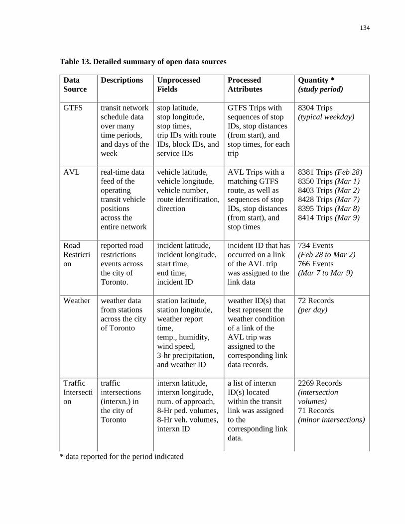
134
Table 13. Detailed summary of open data sources
* data reported for the period indicated
Data
Source
Descriptions Unprocessed
Fields
Processed
Attributes
Quantity *
(study period)
GTFS transit network
schedule data
over many
time periods,
and days of the
week
stop latitude,
stop longitude,
stop times,
trip IDs with route
IDs, block IDs, and
service IDs
GTFS Trips with
sequences of stop
IDs, stop distances
(from start), and
stop times, for each
trip
8304 Trips
(typical weekday)
AVL real-time data
feed of the
operating
transit vehicle
positions
across the
entire network
vehicle latitude,
vehicle longitude,
vehicle number,
route identification,
direction
AVL Trips with a
matching GTFS
route, as well as
sequences of stop
IDs, stop distances
(from start), and
stop times
8381 Trips (Feb 28)
8350 Trips (Mar 1)
8403 Trips (Mar 2)
8428 Trips (Mar 7)
8395 Trips (Mar 8)
8414 Trips (Mar 9)
Road
Restricti
on
reported road
restrictions
events across
the city of
Toronto.
incident latitude,
incident longitude,
start time,
end time,
incident ID
incident ID that has
occurred on a link
of the AVL trip
was assigned to the
link data
734 Events
(Feb 28 to Mar 2)
766 Events
(Mar 7 to Mar 9)
Weather weather data
from stations
across the city
of Toronto
station latitude,
station longitude,
weather report
time,
temp., humidity,
wind speed,
3-hr precipitation,
and weather ID
weather ID(s) that
best represent the
weather condition
of a link of the
AVL trip was
assigned to the
corresponding link
data records.
72 Records
(per day)
Traffic
Intersecti
on
traffic
intersections
(interxn.) in
the city of
Toronto
interxn latitude,
interxn longitude,
num. of approach,
8-Hr ped. volumes,
8-Hr veh. volumes,
interxn ID
a list of interxn
ID(s) located
within the transit
link was assigned
to the
corresponding link
data.
2269 Records
(intersection
volumes)
71 Records
(minor intersections)
135
8.3 Running Speed Model
Based on the two different use case scenarios established in Chapter 3, this thesis tested
running speed models at the route level and at the network level. The route-level running speed
models were designed for the basic analysis use case while the network-level running speed
models were intended for the advanced analysis use case. The variable specifications for each use
cases can be found in section 6.1.2.
As discussed in Chapter 6, the five modelling methods assessed in this study were: multiple
linear regression (MLR), support vector machine (SVM), linear mixed effect (LME), regression
tree (RT), and random forest (RF) models. The definitions for the various error measures, as
presented in section 6.1.4, were used to evaluate model accuracy performance. In addition to model
accuracy, model training time and model prediction time were measured to assess the
computational efficiencies of the models. The compute times were based on i7-7500U processor
with 16GB DDR4, 2400MHz memory, with no GPU acceleration.
8.3.1 Route Level Running Speed Model Results
Four major transit routes were selected for route-level running speed model analysis. Two
bus routes and two streetcar routes were chosen. The first bus route was bus number 34 Eglinton
East serving the east-west Eglinton East Street corridor with subway connections at Eglinton and
Kennedy stations. The second bus route was bus number 54 Lawrence East serving the east-west
Lawrence East Street corridor with rail connections at Eglinton, Lawrence East, and Rouge Hill
Go stations. The 504 King Street streetcar is a TTC streetcar route serving the east-west King
Street corridor. It had shared right of way throughout the route and had subway connections at
Saint Andrew and King Street stations. In contrast, the 512 Saint (St.) Clair streetcar route had
dedicated right of way. It served the east-west St. Clair street corridor and had subway connections
at St. Clair and St. Clair West stations.
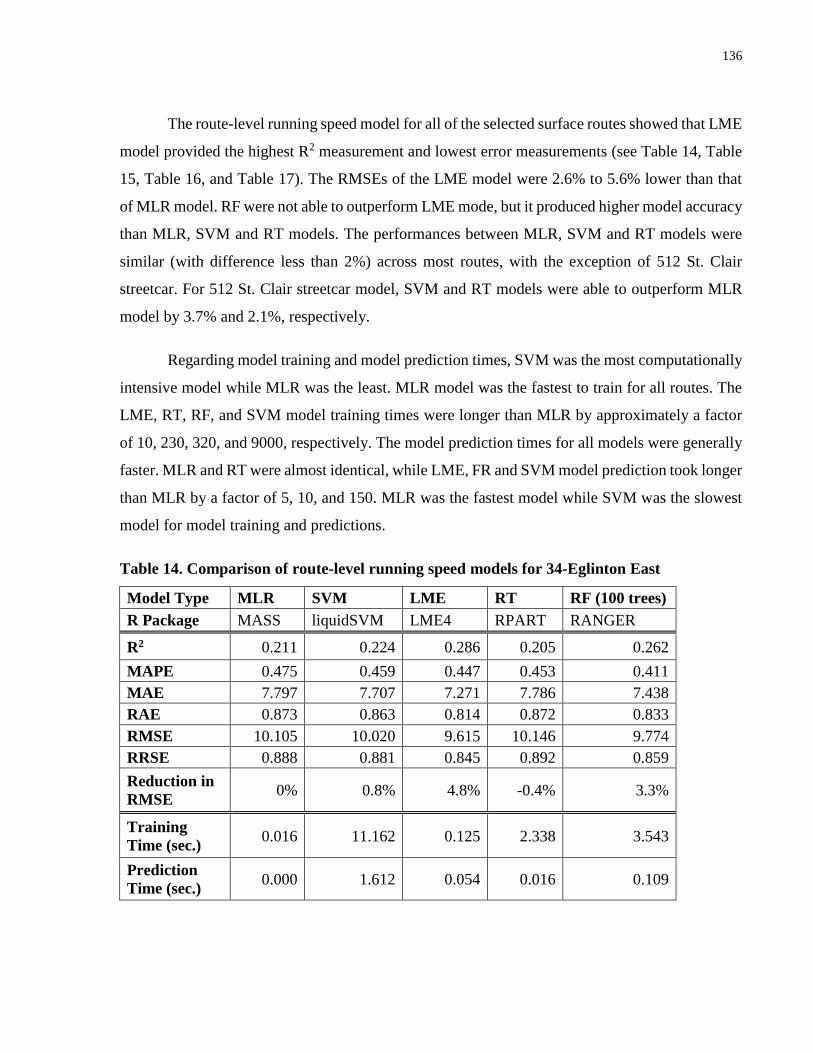
136
The route-level running speed model for all of the selected surface routes showed that LME
model provided the highest R2 measurement and lowest error measurements (see Table 14, Table
15, Table 16, and Table 17). The RMSEs of the LME model were 2.6% to 5.6% lower than that
of MLR model. RF were not able to outperform LME mode, but it produced higher model accuracy
than MLR, SVM and RT models. The performances between MLR, SVM and RT models were
similar (with difference less than 2%) across most routes, with the exception of 512 St. Clair
streetcar. For 512 St. Clair streetcar model, SVM and RT models were able to outperform MLR
model by 3.7% and 2.1%, respectively.
Regarding model training and model prediction times, SVM was the most computationally
intensive model while MLR was the least. MLR model was the fastest to train for all routes. The
LME, RT, RF, and SVM model training times were longer than MLR by approximately a factor
of 10, 230, 320, and 9000, respectively. The model prediction times for all models were generally
faster. MLR and RT were almost identical, while LME, FR and SVM model prediction took longer
than MLR by a factor of 5, 10, and 150. MLR was the fastest model while SVM was the slowest
model for model training and predictions.
Table 14. Comparison of route-level running speed models for 34-Eglinton East
Model Type MLR SVM LME RT RF (100 trees)
R Package MASS liquidSVM LME4 RPART RANGER
R2 0.211 0.224 0.286 0.205 0.262
MAPE 0.475 0.459 0.447 0.453 0.411
MAE 7.797 7.707 7.271 7.786 7.438
RAE 0.873 0.863 0.814 0.872 0.833
RMSE 10.105 10.020 9.615 10.146 9.774
RRSE 0.888 0.881 0.845 0.892 0.859
Reduction in
RMSE 0% 0.8% 4.8% -0.4% 3.3%
Training
Time (sec.) 0.016 11.162 0.125 2.338 3.543
Prediction
Time (sec.) 0.000 1.612 0.054 0.016 0.109

137
Table 15. Comparison of route-level running speed models for 54-Lawrence East
Model Type MLR SVM LME RT RF (100 trees)
R Package MASS liquidSVM LME4 RPART RANGER
R2 0.289 0.307 0.405 0.316 0.344
MAPE 0.397 0.391 0.346 0.380 0.369
MAE 8.208 8.064 7.377 7.969 7.778
RAE 0.830 0.815 0.746 0.806 0.786
RMSE 10.690 10.548 9.773 10.485 10.267
RRSE 0.843 0.832 0.771 0.827 0.810
Reduction in
RMSE 0% 1.3% 8.6% 1.9% 4.0%
Training
Time (sec.) 0.016 15.099 0.194 3.672 7.193
Prediction
Time (sec.) 0.016 2.349 0.064 0.016 0.216
Table 16. Comparison of route-level running speed models for 504-King
Model Type MLR SVM LME RT RF (100 trees)
R Package MASS liquidSVM LME4 RPART RANGER
R2 0.107 0.115 0.223 0.102 0.153
MAPE 0.329 0.326 0.296 0.330 0.318
MAE 5.127 5.077 4.726 5.134 4.982
RAE 0.940 0.931 0.866 0.941 0.913
RMSE 6.816 6.784 6.359 6.834 6.639
RRSE 0.945 0.941 0.882 0.947 0.920
Reduction in
RMSE 0% 0.5% 6.7% -0.3% 2.6%
Training
Time (sec.) 0.017 31.790 0.327 0.662 3.838
Prediction
Time (sec.) 0.011 2.286 0.076 0.012 0.158
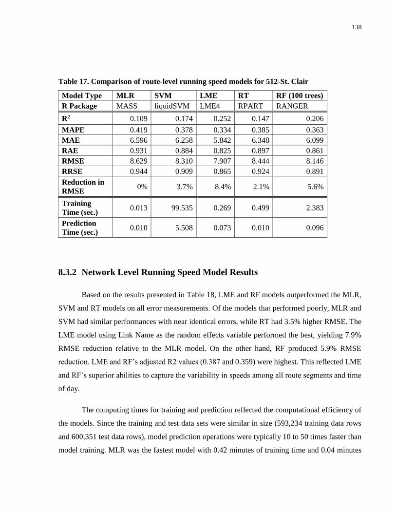
138
Table 17. Comparison of route-level running speed models for 512-St. Clair
Model Type MLR SVM LME RT RF (100 trees)
R Package MASS liquidSVM LME4 RPART RANGER
R2 0.109 0.174 0.252 0.147 0.206
MAPE 0.419 0.378 0.334 0.385 0.363
MAE 6.596 6.258 5.842 6.348 6.099
RAE 0.931 0.884 0.825 0.897 0.861
RMSE 8.629 8.310 7.907 8.444 8.146
RRSE 0.944 0.909 0.865 0.924 0.891
Reduction in
RMSE 0% 3.7% 8.4% 2.1% 5.6%
Training
Time (sec.) 0.013 99.535 0.269 0.499 2.383
Prediction
Time (sec.) 0.010 5.508 0.073 0.010 0.096
8.3.2 Network Level Running Speed Model Results
Based on the results presented in Table 18, LME and RF models outperformed the MLR,
SVM and RT models on all error measurements. Of the models that performed poorly, MLR and
SVM had similar performances with near identical errors, while RT had 3.5% higher RMSE. The
LME model using Link Name as the random effects variable performed the best, yielding 7.9%
RMSE reduction relative to the MLR model. On the other hand, RF produced 5.9% RMSE
reduction. LME and RF’s adjusted R2 values (0.387 and 0.359) were highest. This reflected LME
and RF’s superior abilities to capture the variability in speeds among all route segments and time
of day.
The computing times for training and prediction reflected the computational efficiency of
the models. Since the training and test data sets were similar in size (593,234 training data rows
and 600,351 test data rows), model prediction operations were typically 10 to 50 times faster than
model training. MLR was the fastest model with 0.42 minutes of training time and 0.04 minutes

139
of prediction time. LME and RT were both computationally efficient with less than 3 minutes of
training time and 0.05 minutes of prediction time. SVM was the slowest model with over 36
minutes of training time and 3 minutes of prediction time. RF has a modest training time of 14.69
minutes and prediction time of 0.33 minutes.
Table 18. Comparison of five types of network-level running speed models
Model Type MLR SVM LME RT RF (100 trees)
R Package MASS liquidSVM LME4 RPART RANGER
R2 0.277 0.265 0.387 0.225 0.359
MAPE 0.355 0.358 0.311 0.372 0.325
MAE 7.625 7.677 6.902 7.911 7.109
RAE 0.831 0.837 0.752 0.862 0.775
RMSE 9.950 10.035 9.160 10.303 9.366
RRSE 0.850 0.858 0.783 0.881 0.800
Reduction in
RMSE 0% -0.9% 7.9% -3.5% 5.9%
Training
Time (min.) 0.419 36.272 2.629 1.021 14.681
Prediction
Time (min.) 0.036 3.249 0.049 0.015 0.331

140
8.4 Dwell Time Distribution Model Result
This thesis estimated statistical dwell time models at the stop level assuming that the dwell
time distributions were lognormal. The sigma and mu distribution parameters for the lognormal
distributions were estimated using training data for the case study network. These resulting
parameters were presented on a colour bubble map of the Toronto area (Figure 37). The results of
the lognormal distributions were assessed by comparing the averages and standard deviations of
the observed and predicted dwell times. Finally, the results of the dwell time models were
evaluated using goodness of fit chi-square test.
8.4.1 Log Normal Distribution Parameters
By training a dwell time model for each stop using the training data, the parameters for the
lognormal distributions, mu and sigma, were obtained. The mu parameter is the log average of the
training data. The sigma parameter, also known as the shape parameters, computed the log standard
deviation using the log values and the log average of the training data. The estimation of log normal
distribution parameters was outlined in section 6.2.1.
There was a total of 4488 dwell time models trained for the Toronto network. For each
dwell time model at a stop, a mu and a sigma parameter were obtained. These parameters were
presented as a coloured bubble map (see Figure 37). The colour represented the mu parameter of
log average while the size of the bubble represented the sigma parameter. A small bubble with
green colour indicates a dwell time model with small mu and small sigma parameter values. A
large bubble with red colour indicates a dwell time model with large mu and large sigma parameter
values. The specific values of each dwell time model can be found online via the following URL:
https://bowenwen.carto.com/tables/table_2017_08_12_dwelltimemodel_v5_9/public/map.
The dwell time model parameter values showed variations of dwell time averages and
standard deviations across the transit network. In particular, Figure 37 showed that the mu value
was higher and sigma value was higher for transfer stations at and nearby major subway stations.
The top five subway stations with higher mu and sigma values were:

141
1. Downsview station (mu = 4.63, sigma = 0.82),
2. Rosedale station (mu = 4.54, sigma = 0.69),
3. Broadview station (mu = 4.46, sigma = 1.05),
4. Lawrence East station (mu = 4.43, sigma = 0.95), and
5. Ossington station (mu = 4.42, sigma = 0.88).
In addition to subway stations, dwell time models with large mu and sigma were found for terminal
stations as well. The top five terminal stations with high mu and sigma values were:
1. Main Street station with stop code 14739 (mu = 4.87, sigma = 0.75),
2. Wynford Drive at Don Mills Road with stop code 4720 (mu = 4.83, sigma = 0.83),
3. Ferris Road at Curran Drive with stop code 2475 (mu = 4.74, sigma = 1.03),
4. Lower Jarvis street at Queens Quay East with stop code 6477
(mu = 4.62, sigma = 0.92), and
5. Steeles Avenue West at Highway 27 with stop code 11522 (mu = 4.59, sigma = 0.99).
The dwell time parameter estimates showed variations of averages and standard deviations
across different stops within the network. The dwell time models were used to predict dwell
times during simulation.

142
Figure 37. Dwell time model parameters at stops on coloured bubble map
8.4.2 Dwell Time Model Evaluations
Dwell time models that represent the stochasticity of dwell times across different stops well
should replicate the variation of observed dwell time averages and standard deviations. A
comparison between the dwell time predictions and observed dwell times at each stop for the
simulated period was made. Furthermore, a chi-squared test was used to evaluate the goodness of
fit of the dwell time model at the network level.

143
8.4.2.1 Observed versus Predicted Dwell Times
The observed dwell time coloured bubble plot showed the variation in dwell times across
the network. The observed dwell times were obtained from the 1-day test data for simulation. The
colour of the bubble represented the observed dwell time averages while the size of the bubble
indicated the standard deviations. Figure 38 showed that most of the stops along many corridors
have low observed averages and standard deviations in dwell times. However, the stops with major
transfers with other bus or streetcar routes and the subway system have larger averages and
standard deviations in dwell times. In particular, stops at the subway stations have larger values.
For example, many of the stops at the subway stations on Yonge Street, University Avenue, and
Bloor Street had larger averages and standard deviations of dwell times. In addition, terminal stops
for transit routes were observed to have high averages and standard deviations of dwell time values.
The predicted dwell time coloured bubble plot was obtained using dwell time models with
distribution draws performed at simulation run times (see Figure 39). The predicted dwell time
results were obtained using seed 100 during simulation to ensure simulation model results were
comparable between different running speed models. The predicted dwell time model results
showed variations in dwell time across the network. Stops at subway stations yielded larger
averages and standard deviations of predicted dwell times. These stops were on the Yonge Street,
University Avenue, and Bloor Street corridors. Further away from the Toronto downtown region,
larger averages and standard deviations of predicted dwell times were observed for terminal stop
stations.
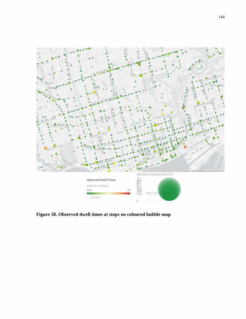
144
Figure 38. Observed dwell times at stops on coloured bubble map
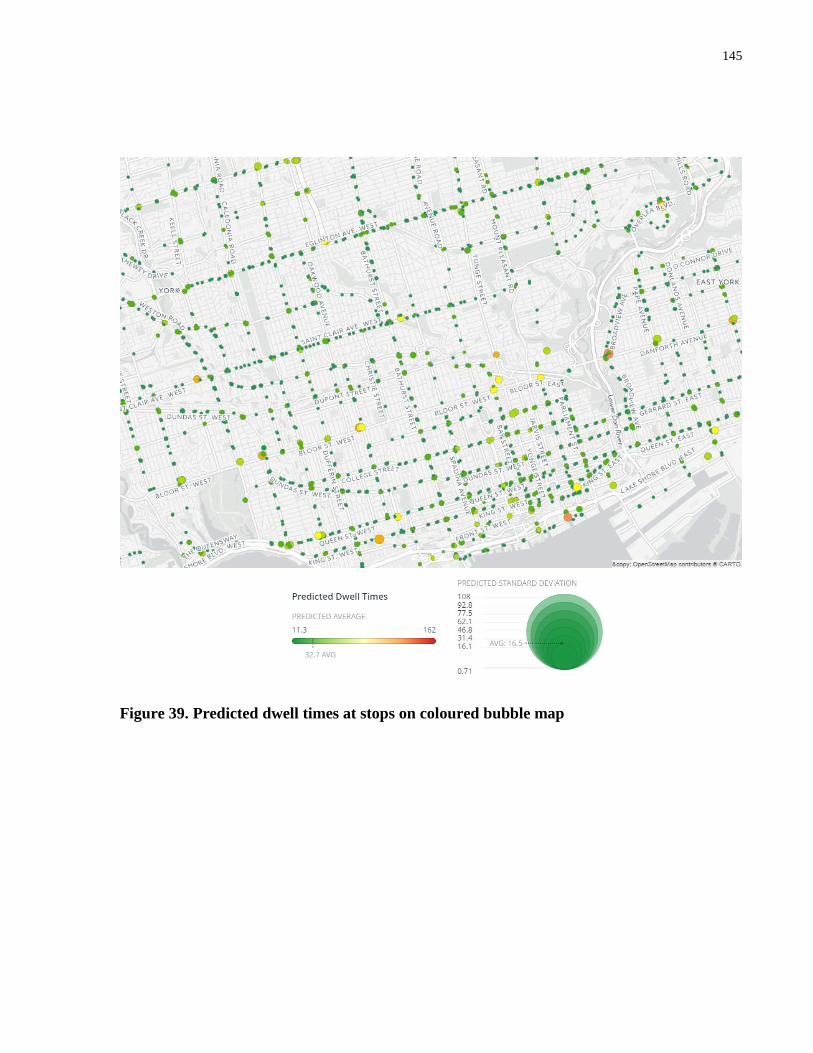
145
Figure 39. Predicted dwell times at stops on coloured bubble map
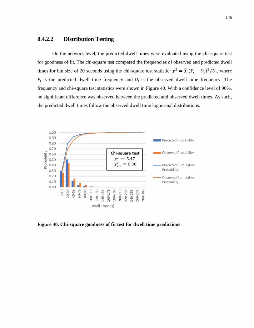
146
8.4.2.2 Distribution Testing
On the network level, the predicted dwell times were evaluated using the chi-square test
for goodness of fit. The chi-square test compared the frequencies of observed and predicted dwell
times for bin size of 20 seconds using the chi-square test statistic: 𝜒2 = ∑ (𝑃𝑖 − 𝑂𝑖)2 𝑂𝑖⁄ , where
𝑃𝑖 is the predicted dwell time frequency and 𝑂𝑖 is the observed dwell time frequency. The
frequency and chi-square test statistics were shown in Figure 40. With a confidence level of 90%,
no significant difference was observed between the predicted and observed dwell times. As such,
the predicted dwell times follow the observed dwell time lognormal distributions.
Figure 40. Chi-square goodness of fit test for dwell time predictions
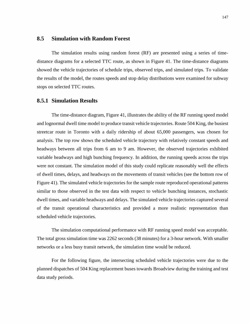
147
8.5 Simulation with Random Forest
The simulation results using random forest (RF) are presented using a series of time-
distance diagrams for a selected TTC route, as shown in Figure 41. The time-distance diagrams
showed the vehicle trajectories of schedule trips, observed trips, and simulated trips. To validate
the results of the model, the routes speeds and stop delay distributions were examined for subway
stops on selected TTC routes.
8.5.1 Simulation Results
The time-distance diagram, Figure 41, illustrates the ability of the RF running speed model
and lognormal dwell time model to produce transit vehicle trajectories. Route 504 King, the busiest
streetcar route in Toronto with a daily ridership of about 65,000 passengers, was chosen for
analysis. The top row shows the scheduled vehicle trajectory with relatively constant speeds and
headways between all trips from 6 am to 9 am. However, the observed trajectories exhibited
variable headways and high bunching frequency. In addition, the running speeds across the trips
were not constant. The simulation model of this study could replicate reasonably well the effects
of dwell times, delays, and headways on the movements of transit vehicles (see the bottom row of
Figure 41). The simulated vehicle trajectories for the sample route reproduced operational patterns
similar to those observed in the test data with respect to vehicle bunching instances, stochastic
dwell times, and variable headways and delays. The simulated vehicle trajectories captured several
of the transit operational characteristics and provided a more realistic representation than
scheduled vehicle trajectories.
The simulation computational performance with RF running speed model was acceptable.
The total gross simulation time was 2262 seconds (38 minutes) for a 3-hour network. With smaller
networks or a less busy transit network, the simulation time would be reduced.
For the following figure, the intersecting scheduled vehicle trajectories were due to the
planned dispatches of 504 King replacement buses towards Broadview during the training and test
data study periods.
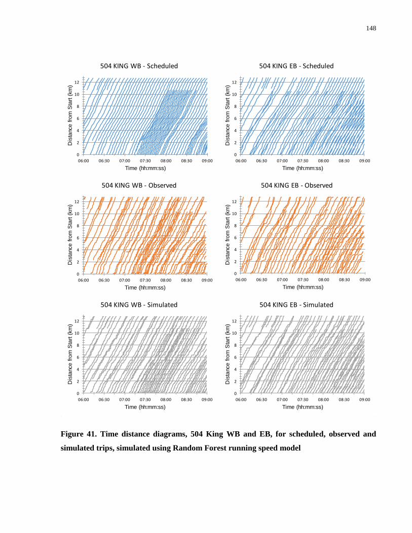
148
Figure 41. Time distance diagrams, 504 King WB and EB, for scheduled, observed and
simulated trips, simulated using Random Forest running speed model
0
2
4
6
8
10
12
06:00 06:30 07:00 07:30 08:00 08:30 09:00
Dis
tance
fro
m S
tart
(km
)
Time (hh:mm:ss)
504 KING WB - Scheduled
0
2
4
6
8
10
12
06:00 06:30 07:00 07:30 08:00 08:30 09:00
Dis
tance
fro
m S
tart
(km
)
Time (hh:mm:ss)
504 KING WB - Observed
0
2
4
6
8
10
12
06:00 06:30 07:00 07:30 08:00 08:30 09:00
Dis
tance
fro
m S
tart
(km
)
Time (hh:mm:ss)
504 KING WB - Simulated
0
2
4
6
8
10
12
06:00 06:30 07:00 07:30 08:00 08:30 09:00
Dis
tance
fro
m S
tart
(km
)
Time (hh:mm:ss)
504 KING EB - Simulated
0
2
4
6
8
10
12
06:00 06:30 07:00 07:30 08:00 08:30 09:00
Dis
tance
fro
m S
tart
(km
)
Time (hh:mm:ss)
504 KING EB - Observed
0
2
4
6
8
10
12
06:00 06:30 07:00 07:30 08:00 08:30 09:00
Dis
tance
fro
m S
tart
(km
)
Time (hh:mm:ss)
504 KING EB - Scheduled

149
8.5.2 Route-based Validation
The route speed of a transit vehicle is important for the planning of transit services as it
determines the number of transit units and the frequency of service. The distribution of route
speeds of the simulated trips, generated by the RF running speed model, was examined to
demonstrate the ability of the simulation model to replicate the observed conditions (see Figure 43
for results of two major bus routes and two streetcar routes). While the schedule-based route speeds
exhibited low variability for each branch of a route, the simulated route speeds varied across
different trips and better reflected the observed conditions. However, the distributions between
simulated and observed route speeds were not identical. In general, the simulated route speeds
were more normally distributed with smaller variances. The average route speeds between the
simulated and observed trips matched well for most routes.
Figure 42. Route speed validation for four major TTC routes, simulated using Random
Forest running speed model

150
8.5.3 Station-based Validation
The delays at each stop are critical for the coordination of transfers as well as crowding at
major transfer stations. This study assessed the distributions of delays captured at 14 major transfer
stops, at subway stations, of four feeder bus and streetcar routes, using the kernel density
estimation for data smoothing. While only a few stops had near identical simulated and observed
distribution, the simulation model was able to capture either the average of delays or the shape of
the density for most stops. For stops where the center of delay distribution curve was shifted, such
as the stops for 504 King EB, the route speed distribution was also shifted. The shape of the
distributions did not match well for 512 St Clair. In addition, routes with less similar variances of
route speeds also have delay density shapes that do not match as well. Even though the simulated
models do not replicate identically the stop delay distribution as observed, they did provide a
reasonable representation of the delays experienced.
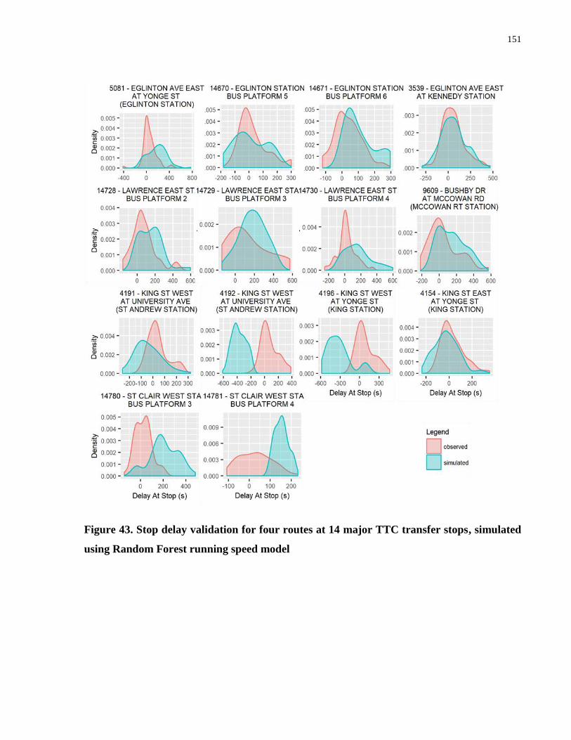
151
Figure 43. Stop delay validation for four routes at 14 major TTC transfer stops, simulated
using Random Forest running speed model

152
8.6 Simulation with Linear Mixed Effect Model
Using the linear mixed effects (LME) running speed model, simulated vehicle movements
were generated. The vehicle movements were presented as a series of time-distance diagrams for
a selected TTC route. The vehicle trajectories of schedule trips, observed trips, and simulated trips
are shown on the time-distance diagrams (Figure 44). The simulated routes speeds and stop delay
distributions were validated against the observed values for subway stops on selected TTC routes.
8.6.1 Simulation Results
The vehicle movements generated by the LME running speed model and lognormal dwell
time model were presented as a series of time-distance diagrams (Figure 44). Similar to the results
for the RF running speed model, the busy streetcar route 504 King was chosen for analysis. The
scheduled vehicle trajectory (top row) showed constant speeds and headways between all trips
from 6 am to 9 am. This did not model the observed trajectories that had variable headways and
high bunching frequency. The LME running speeds model was able to produce non-constant
running speeds across the trips, as observed. The simulation model using LME replicated the
effects of dwell times, delays, and headways on vehicle movements, (refer to bottom row of Figure
41). Operational patterns with vehicle bunching, stochastic dwell times, and variable headways
and delays were reproduced by the LME running speed model. The simulated vehicle trajectories
captured several of the transit operational characteristics and provided a more realistic
representation than scheduled vehicle trajectories.
The simulation computational performance with LME running speed model was
acceptable. For a 3-hour TTC network, the total gross simulation time was 1304 seconds (22
minutes). With smaller networks or a less busy transit network, the simulation time could be less.
For the following figure, the intersecting scheduled vehicle trajectories were due to the
planned dispatches of 504 King replacement bus towards Broadview during the training and test
data study periods.
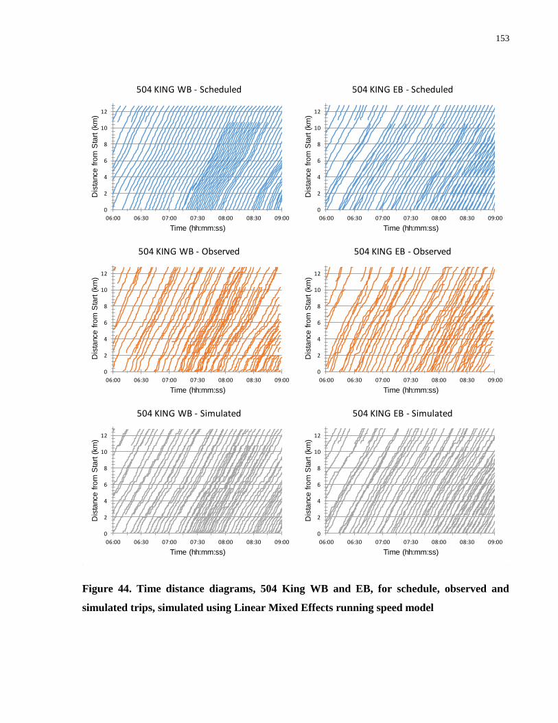
153
Figure 44. Time distance diagrams, 504 King WB and EB, for schedule, observed and
simulated trips, simulated using Linear Mixed Effects running speed model
0
2
4
6
8
10
12
06:00 06:30 07:00 07:30 08:00 08:30 09:00
Dis
tance
fro
m S
tart
(km
)
Time (hh:mm:ss)
504 KING EB - Scheduled
0
2
4
6
8
10
12
06:00 06:30 07:00 07:30 08:00 08:30 09:00
Dis
tance
fro
m S
tart
(km
)
Time (hh:mm:ss)
504 KING WB - Scheduled
0
2
4
6
8
10
12
06:00 06:30 07:00 07:30 08:00 08:30 09:00
Dis
tance
fro
m S
tart
(km
)
Time (hh:mm:ss)
504 KING WB - Observed
0
2
4
6
8
10
12
06:00 06:30 07:00 07:30 08:00 08:30 09:00
Dis
tance
fro
m S
tart
(km
)
Time (hh:mm:ss)
504 KING WB - Simulated
0
2
4
6
8
10
12
06:00 06:30 07:00 07:30 08:00 08:30 09:00
Dis
tance
fro
m S
tart
(km
)
Time (hh:mm:ss)
504 KING EB - Observed
0
2
4
6
8
10
12
06:00 06:30 07:00 07:30 08:00 08:30 09:00
Dis
tance
fro
m S
tart
(km
)
Time (hh:mm:ss)
504 KING EB - Simulated

154
8.6.2 Route-based Validation
Route speeds are important for the planning of transit services, so its distribution was
chosen as a validation measure for the simulation model. The distribution of route speeds of the
simulated trips, generated using the LME model, was examined to demonstrate the ability of the
simulation model to replicate the observed conditions. The results for Eglinton and Lawrence East
buses and Saint Clair and King Streetcars were summarized by a series of route speed histograms
(see Figure 45). While the schedule-based route speeds exhibited low variability for each branch
of a route, the simulated route speeds varied across different trips and better reflected the observed
conditions. However, the distributions between simulated and observed route speeds were not
identical. In general, the simulated route speeds were more normally distributed with smaller
variances. The average route speeds between the simulated and observed trips matched well for
most routes.
Figure 45. Route speed validation for four major TTC routes, simulated using Linear Mixed
Effects running speed model

155
8.6.3 Station-based Validation
Scheduled transit services usually optimize the crowding and the coordination of transfers
at major stations, and delays can often have adverse effect on crowding and transfer. The
distribution of delays at 14 major subway transfer stops along four major feeder bus and streetcar
routes were generated. The distributions were produced using the kernel density estimation for
data smoothing. It was found that only few stops had near identical simulated and observed
distribution. However, the shapes and/or averages of the delay distributions were captured for
some stops. For stops where the center of delay distribution curve was shifted, such as the stops
for 504 King EB, the route speed distribution was also shifted. The distribution for different bus
platforms at the same station, such as those for 512 St Clair, could yield different results as well.
For instance, the delay distribution for bus platform 3 matched better than that for bus platform 4
at St Clair station. Even though the simulated models did not replicate identically the stop delay
distribution as observed, they did provide a reasonable representation of the delays experienced.

156
Figure 46. Stop delay validation for four routes at 14 major TTC transfer stops, simulated
using Linear Mixed Effects running speed model
157
8.7 Summary
This chapter presented data-driven mesoscopic transit simulation models for the Toronto
Transit Commission case study. The mesoscopic transit simulation model was made up of a
regression running speed model and a lognormal statistical dwell time model. In the case study
presented in this thesis, five different regression models for running speed were evaluated. The
random forest and linear mixed effect models were found to provide higher model accuracy and
reasonable computational efficiencies for application. The superior performances of the random
forest and linear mixed effect models were consistent for route-level and network-level running
speed models. The dwell time models were also evaluated based on their ability to replicate dwell
times variation across different stops in the network. The dwell time models were able to capture
the higher dwell time averages and larger standard deviations for major transfer stops intersecting
subway lines. A chi-square goodness of fit test was performed for dwell times at the network level.
It was found that the dwell time distributions pass this statistical test with 90% confidence.
Using the estimated running speed and dwell time models, mesoscopic transit simulations
were performed using the random forest and linear mixed effect running speed models. The
random dwell time distribution draws from the dwell time models were controlled using a seed
with a value of 100 during simulation runs in order to ensure comparability. This chapter presented
the simulation results for both models by showing the vehicle trajectories of a selected TTC route
on a series of time-distance diagrams. In addition, validations were performed on the simulation
results for four major feeder bus and streetcar routes. The route-based validation examined the
distribution of route speeds between scheduled, observed, and simulated trips. The stop-based
validation compared the distributions of stop delay values at major TTC subway stops along the
four major routes. The vehicle trajectories generated by the models were reasonably realistic, and
provided drastic improvements over the scheduled trajectories. The validations results, however,
did not show identically matched distribution results, which replicated the stochasticity of the
transit operational characteristics reasonably well. The overall results of the simulation were
logical and promising.
158
Chapter 9
Conclusion
This thesis provided a framework to construct a data-driven surface transit simulator using
multiple open data sources. It was shown that by combining the use of GTFS, AVL, road
restriction, weather, and signalized intersection data, a data-driven transit movement simulation
model could be constructed using statistical models of running speeds and dwell times. The
conclusions reached based on the model results contributed to a better understanding of the data-
driven models for transit simulation. The research accomplishments presented throughout this
thesis are detailed in the research contribution section. Finally, future research directions to
improve the simulation model, to extend its capabilities, and to apply it to real world systems are
discussed.
9.1 Summary of Results
Data-driven simulation models require accurate running speed and dwell time models to
realistically predict the movement of transit vehicles across a network. A detailed summary of the
running speed models and dwell time models contributed to a better understanding of the transit
simulation model results. A summary of the validation results helped in identifying many potential
future research directions.
9.1.1 Running Speed Models
Even though the model specifications for route-level and network-level running speed
models were different, the relative performances of the models were similar. The linear mixed
effects (LME) method produced the best model prediction performances with the highest R2 and
lowest error measurements. The random forest (RF) model came a close second in model

159
prediction performances with 2% more errors for the network-level model. RF was about 10 times
slower on average than LME at model training and predictions. Based on the route-level and
network-level model results, the training time for LME with more variables and more training data
took considerably longer. Such an increase in training time was less severe for RF, nonetheless the
training time for RF is still more than LME. Prediction with RF took considerably longer with a
larger training sample. Complex and deeper trees with larger training data resulted in an
exponential increase in prediction times with RF. In contrast, the prediction time with LME
increased linearly. This is consistent with the understanding that predictions with LME depend
only on the complexity of variable specifications, not sample sizes. The differences in training and
prediction time characteristics, as well as model accuracies are important considerations for
simulation applications.
The RF may be considered for model simulation applications, despite the superior
prediction performance of LME, because it provides more flexible implementation. Since the LME
model used link name as the random effects variable, it cannot be applied to links with no recorded
training data. In contrast, the RF model can handle clustered data with similar link characteristics
without having the link names explicitly specified. For simulations requiring implementations of
new links, RF model would be preferred as it could predict running speeds for similar links to that
it was trained on.
Unlike RF, LME does not suffer from increased model complexity due to larger datasets
and deeper trees. This results in a more stable model prediction time for LME that increases
linearly with network size. Although the LME model training became slower with more complex
variable specification, it was a more computationally efficient modelling method than RF with
notably better model performance. However, unlike RF, LME requires a random effect variable of
link name, which makes implementation of the LME model for new links difficult. If the addition
of new links was not needed and the data sizes were large, LME should be the preferred model.
160
9.1.2 Dwell Time Models
The predicted dwell times generated using the dwell time models replicated the patterns of
the observed dwell times well. In particular, the predicted values captured longer dwell times with
higher variance nearby or at subway stations and terminal transit stops. The higher passenger
demand for boarding and alighting at transfer stations could explain the longer dwell times with
higher variance at the subway stations. The longer dwell times at terminal stations could be
explained by the higher passenger demand at the area. For example, the Main Street station on
Danforth Avenue had higher average and standard deviation of dwell times because the station
was a major transfer point between the 506 Carlton streetcar, subway transfer to line 2, and several
buses. On the other hand, some of the terminal stops such as Lower Jarvis Street at Queens Quay
East, Wynford Drive at Don Mills Road, and Gunns Loop at St Clair Avenue West do not have
heavy passenger demands. Such discrepancy may be due to the way that automatic vehicle location
(AVL) data were recorded at terminal stations. It was unclear if all drivers follow the same protocol
of changing the vehicle head sign the moment the vehicle arrives at the terminal station. In
addition, the dwell times at terminal stations may contain waiting time for the start of its next trip,
in addition to the boarding and alighting times. This should not affect simulation significantly
because dwell times for on-time arrivals at the terminal stop rarely affect the departure time of the
next trip, given the previous trip arrived early. The behaviour of bus and streetcar waiting at the
terminal stop for its next scheduled trip departure is an important assumption built into the
simulation and can overcome this limitation associated with the dwell time model. The lognormal
dwell time model used in this study replicated the observed dwell time distributions well; however,
there are a few issues which may have affected the model fit. Since the available AVL data had a
20-second resolution, some lower values of dwell times would not be captured, especially for parts
of the networks with poor GPS signal reception, such as areas with tall buildings and tree cover.
This may have led to biased data points, resulting in slightly left skewed observed dwell time
distribution when compared to the simulated values.

161
9.1.3 Simulation Models
The simulation of transit movements was illustrated using the results based on running
speed and dwell time predictions with a “base case” GTFS schedule simulation scenario. This
thesis investigated the performances of the RF and LME running speed models. The results of the
simulated vehicle movements were assessed using a series of time-distance diagrams. Then, the
simulated vehicle movements were validated at the route and the stop levels.
The simulated vehicle trajectories were more realistic than the scheduled vehicle
trajectories. Based on the results on vehicle trajectories, both RF and LME were able to capture
vehicle bunching, distributions of dwell times, stochastic patterns of delay and variations in
headways. The results of RF and LME simulation models were similar. Unlike the observed data,
simulated vehicle trips showed more stable running speeds. The instability of running speed in the
observed vehicle trips could be the result of stochastic traffic congestion. However, even without
traffic congestion data, the patterns of transit travel were replicated generally well by the RF and
LME models. The data-driven models can be a viable way to simulate transit movements
efficiently.
The results of the data-driven simulation were validated at the route level and stop level.
While the simulated route speeds were more realistic than the scheduled route speeds, the
simulated and observed distributions were not identical. The simulated route speeds were more
normally distributed with lower variance than the observed route speeds. This could be due to
unknown disruptions, such as congestion, signal delays, or short-turned transit trips, which may
have shifted the observed route speed distributions and induced larger variance. This affected the
stop delay distributions, as evident in the shift in the means and variances of some stop delay
curves. The simulated trips captured the statistical variations of route speeds and stop delays much
better than the scheduled trips; however, additional data on congestion and transit disruptions
could potentially improve model fit.
While the simulation results from RF and LME were similar, LME is more computationally
efficient with half of the simulation time as RF. The simulation times for both methods were

162
reasonable. In choosing whether to use RF or LME for simulation applications, the need to create
new links with existing link characteristics needs to be assessed. Since RF provides a more flexible
implementation of new links, it may be preferred over LME despite the higher computational cost.
However, if only the modelling of existing transit links is needed, LME should be the preferred
choice given its computational efficiency.
9.2 Research Contributions
This thesis presented an innovative and data-driven approach to transit simulations and it
provided significant contributions on many aspects of this approach. The data-driven transit
simulation used open source data to model surface transit movements with running speed models
and dwell time models. Using this modelling framework, this thesis collected and processed
multiple open source data to obtain variables required for modelling. Using GTFS schedule data,
the AVL data was processed into trips to generate stop-based variables such as stop arrival times,
dwell times, delays, and headways. Then, the spatiotemporal matching of the AVL trip data to
additional sources of open data such as weather, road restrictions, and signalized intersections data
provided policy-relevant variables for model estimation. These processed AVL data enabled the
modelling of running speed and dwell time. The second key contribution was the use of structured
data from multiple data sources to model running speed and dwell times. This thesis performed a
thorough comparison of different machine learning algorithms to model stop-to-stop transit
running speeds. It was shown that random forest and linear mixed effect models were most suitable
for network-level running speed models, and the lognormal dwell time distribution modelled dwell
time variations across the network well. Thirdly, this thesis developed a simulation procedure for
data-driven simulation, with standardized analytics reports. This research contribution lays the
foundation for event-based data-driven simulations and allows future researchers to explore ways
to further optimize data-driven simulation for large-scale network applications. Finally, this thesis
demonstrated the capabilities of the data-driven simulation using a case study on the Toronto
network.

163
9.3 Future Research
This study demonstrated an innovative concept for transit simulation using data-driven
machine learning models. These initial simulation results illustrate the need to incorporate
congestion in future studies to more accurately capture route speeds and stop delays. In addition,
more complex simulation scenarios could improve the realism of the simulation output as well.
Large transit agencies such as the TTC make changes to their services on a daily basis to address
transit disruptions and ease network congestion. Surface transit operational changes such as short-
turned trips or temporary shuttle buses could be useful to incorporate in future simulation models.
In future studies, advanced dwell time models that incorporate passenger demand data from
automatic fare payment or automatic passenger counter systems could be used to capture the effect
crowding and dwell times on transit movements. Advanced dwell time models could handle more
complex scenarios with varying passenger demand. For example, the effects of stop additions,
relocations, and removals could be assessed by reallocating passenger demand among stops.
To further enhance the benefits of more advanced dwell time models, software integration
with pedestrian and station models could further improve the realism of the simulation model by
representing changing passenger demands across the different modes of transit. Such integration
may require the synchronization of time steps during the iterative prediction procedure to allow
simultaneous updates. The conversion of the current event-based running speed prediction
procedure to time-step-based requires further software development efforts.
Finally, the use of continuous learning algorithms to provide real-time transit simulation
models could enable transit agencies to quantify and optimize the effects of operational decisions.
A key benefit of data-driven simulation model is that there was no need to construct a model from
the ground up. The simulation pipeline presented in this thesis could be converted into a continuous
learning application where the data download and data processing could take place continuously
to update the estimated running speed and dwell time models. Future research could use continuous
learning modelling methods to create online transit simulation models.

164
Bibliography
Allen, M. P. (1997). The coefficient of determination in multiple regression. In Understanding
Regression Analysis (pp. 91–95). Springer, Boston, MA. https://doi.org/10.1007/978-0-
585-25657-3_19
Bahuleyan, H., & Vanajakshi, L. D. (2017). Arterial Path-Level Travel-Time Estimation Using
Machine-Learning Techniques. Journal of Computing in Civil Engineering, 31(3).
https://doi.org/10.1061/(ASCE)CP.1943-5487.0000644
Bai, C., Peng, Z.-R., Lu, Q.-C., & Sun, J. (2015). Dynamic Bus Travel Time Prediction Models
on Road with Multiple Bus Routes. Computational Intelligence and Neuroscience, 2015,
e432389. https://doi.org/10.1155/2015/432389
Balakrishna, P., Raman, S., Trafalis, T. B., & Santosa, B. (2008). Support vector regression for
determining the minimum zone sphericity. The International Journal of Advanced
Manufacturing Technology, 35(9–10), 916–923. https://doi.org/10.1007/s00170-006-
0774-1
Bates, D., Maechler, M., Bolker, B., Walker, S., Christensen, R. H. B., Singmann, H., … Green,
P. (2017, April 19). Linear Mixed-Effects Models using “Eigen” and S4 (Package
“lme4”). CRAN Repository. Retrieved from https://cran.r-
project.org/web/packages/lme4/lme4.pdf

165
Berk, R. A. (2008). Classification and Regression Trees (CART). In Statistical Learning from a
Regression Perspective (pp. 1–65). Springer, New York, NY.
https://doi.org/10.1007/978-0-387-77501-2_3
Bernstein, M. N. (2015, August 29). The Radial Basis Function Kernel. University of Wisconsin
- Madison. Retrieved from
http://pages.cs.wisc.edu/~matthewb/pages/notes/pdf/svms/RBFKernel.pdf
Breiman, L. (2001). Random Forests. Machine Learning, 45(1), 5–32.
https://doi.org/10.1023/A:1010933404324
Caruana, R., & Niculescu-Mizil, A. (2006). An Empirical Comparison of Supervised Learning
Algorithms. In Proceedings of the 23rd International Conference on Machine Learning
(pp. 161–168). New York, NY, USA: ACM. https://doi.org/10.1145/1143844.1143865
Casas, J., Perarnau, J., & Torday, A. (2011). The need to combine different traffic modelling
levels for effectively tackling large-scale projects adding a hybrid meso/micro approach.
Procedia - Social and Behavioral Sciences, 20, 251–262.
https://doi.org/10.1016/j.sbspro.2011.08.031
Catala, M., Dowling, S., & Hayward, D. (2011). Expanding the Google Transit Feed
Specification to Support Operations and Planning. Retrieved from
https://trid.trb.org/view.aspx?id=1127545

166
Cats, O., Burghout, W., Toledo, T., & Koutsopoulos, H. (2010). Mesoscopic Modeling of Bus
Public Transportation. Transportation Research Record: Journal of the Transportation
Research Board, 2188, 9–18. https://doi.org/10.3141/2188-02
Chai, T., & Draxler, R. R. (2014). Root mean square error (RMSE) or mean absolute error
(MAE)? – Arguments against avoiding RMSE in the literature. Geosci. Model Dev., 7(3),
1247–1250. https://doi.org/10.5194/gmd-7-1247-2014
Charpentier, A. (2013, January 27). Regression tree using Gini’s index. Retrieved May 19, 2017,
from http://freakonometrics.hypotheses.org/1279
Chen, M., Yu, L., Zhang, Y., & Guo, J. (2009). Analyzing urban bus service reliability at the
stop, route, and network levels. Transportation Research Part A: Policy and Practice,
43(8), 722–734. https://doi.org/10.1016/j.tra.2009.07.006
Chen, X., Liu, X., Xia, J., & Chien, S. I. (2004). A Dynamic Bus-Arrival Time Prediction Model
Based on APC Data. Computer-Aided Civil and Infrastructure Engineering, 19(5), 364–
376. https://doi.org/10.1111/j.1467-8667.2004.00363.x
Christoph Rüegg, Marcus Cuda, Jurgen Van Gael, Scott Stephens, Alexander Karatarakis, Eirik
Ovegard, … Gustavo Guerra. (2017, July 16). Math.NET Numerics. Retrieved September
20, 2017, from https://numerics.mathdotnet.com/
City of Toronto. (2015, October 7). Road Restrictions. Retrieved July 10, 2017, from
https://www1.toronto.ca/wps/portal/contentonly?vgnextoid=1af0e69ae554e410VgnVCM
10000071d60f89RCRD

167
City of Toronto. (2017a). TTC Routes and Schedules - Open Data Toronto. Retrieved September
22, 2017, from
https://www1.toronto.ca/wps/portal/contentonly?vgnextoid=96f236899e02b210VgnVC
M1000003dd60f89RCRD
City of Toronto. (2017b, April 19). Traffic Signal Vehicle and Pedestrian Volumes. Retrieved
April 19, 2017, from
http://www1.toronto.ca/wps/portal/contentonly?vgnextoid=417aed3c99cc7310VgnVCM
1000003dd60f89RCRD
City of Toronto. (2017c, April 19). Traffic Signals Tabular. Retrieved April 19, 2017, from
http://www1.toronto.ca/wps/portal/contentonly?vgnextoid=965b868b5535b210VgnVCM
1000003dd60f89RCRD
Cortés, C., Pagès, L., & Jayakrishnan, R. (2005). Microsimulation of Flexible Transit System
Designs in Realistic Urban Networks. Transportation Research Record: Journal of the
Transportation Research Board, 1923, 153–163. https://doi.org/10.3141/1923-17
Cortes, C., & Vapnik, V. (1995). Support-Vector Networks. Mach. Learn., 20(3), 273–297.
https://doi.org/10.1023/A:1022627411411
Elhenawy, M., Chen, H., & Rakha, H. A. (2014). Random Forest Travel Time Prediction
Algorithm Using Spatiotemporal Speed Measurements. Presented at the 21st Intelligent
Transportation Systems World Congress Conference Proceedings. Retrieved from

168
http://itswc.conferencespot.org/56062-itsa-1.1291464/t-005-1.1292028/f-023-
1.1292111/ts55-1.1292075/12307-1.1292120?qr=1
Farid, Y. Z., Christofa, E., & Paget-Seekins, L. (2016). Estimation of Short-Term Bus Travel
Time by Using Low-Resolution Automated Vehicle Location Data. Transportation
Research Record: Journal of the Transportation Research Board, 2539, 113–118.
https://doi.org/10.3141/2539-13
Fernandez, R., Cortes, C., & Burgos, V. (2010). Microscopic simulation of transit operations:
policy studies with the MISTRANSIT application programming interface. Transportation
Planning and Technology, 33(2), 157–176.
Gaudette, P., Chapleau, R., & Spurr, T. (2016). Bus Network Microsimulation with General
Transit Feed Specification and Tap-in-Only Smart Card Data. Transportation Research
Record: Journal of the Transportation Research Board, (2544). Retrieved from
https://trid.trb.org/view.aspx?id=1393935
Goldstein, B., & Dyson, L. (Eds.). (2013). Beyond transparency: open data and the future of
civic innovation. San Francisco: Code for America Press.
Google Inc. (2016, July 12). Overview | Static Transit. Retrieved August 8, 2017, from
https://developers.google.com/transit/gtfs/reference/
Gumedze, F. N., & Dunne, T. T. (2011). Parameter estimation and inference in the linear mixed
model. Linear Algebra and Its Applications, 435(8), 1920–1944.
https://doi.org/10.1016/j.laa.2011.04.015
169
Harvey, A. C. (1990). Forecasting, Structural Time Series Models and the Kalman Filter.
Cambridge University Press.
Hastie, T., Friedman, J., & Tibshirani, R. (2008). The Elements of Statistical Learning: Data
Mining, Inference, and Prediction (2nd ed). Stanford, California: Springer.
Hoch, T. (2015). An Ensemble Learning Approach for the Kaggle Taxi Travel Time Prediction
Challenge. In Proceedings of the 2015th International Conference on ECML PKDD
Discovery Challenge - Volume 1526 (pp. 52–62). Aachen, Germany, Germany: CEUR-
WS.org. Retrieved from http://dl.acm.org/citation.cfm?id=3056172.3056179
Hsu, C.-W., Chang, C.-C., & Lin, C.-J. (2016, May 19). A Practical Guide to Support Vector
Classification. National Taiwan University. Retrieved from
http://www.csie.ntu.edu.tw/~cjlin/papers/guide/guide.pdf
Hu, C., Zhou, B., & Hu, J. (2014). Fast Support Vector Data Description training using edge
detection on large datasets. In 2014 International Joint Conference on Neural Networks
(IJCNN) (pp. 2176–2182). https://doi.org/10.1109/IJCNN.2014.6889718
Hu, W. X., & Shalaby, A. (2017). Use of Automated Vehicle Location Data for Route- and
Segment-Level Analyses of Bus Route Reliability and Speed. Transportation Research
Record: Journal of the Transportation Research Board, 2649, 9–19.
https://doi.org/10.3141/2649-02
Jean-Michel Perraud. (2015, August 8). R.NET. Retrieved July 31, 2017, from
https://rdotnet.codeplex.com/Wikipage?ProjectName=rdotnet

170
Jeong, R., & Rilett, R. (2004). Bus arrival time prediction using artificial neural network model.
In Proceedings. The 7th International IEEE Conference on Intelligent Transportation
Systems (IEEE Cat. No.04TH8749) (pp. 988–993).
https://doi.org/10.1109/ITSC.2004.1399041
Kormaksson, M., Barbosa, L., Vieira, M. R., & Zadrozny, B. (2014). Bus Travel Time
Predictions Using Additive Models. arXiv:1411.7973 [Cs, Stat], 875–880.
https://doi.org/10.1109/ICDM.2014.107
Kucirek, P. (2012, September). Comparison between MATSim & EMME: Developing a
Dynamic, Activity-based Microsimulation Transit Assignment Model for Toronto.
University of Toronto, Toronto, ON. Retrieved from
https://tspace.library.utoronto.ca/bitstream/1807/33277/10/Kucirek_Peter_201211_MASc
_thesis.pdf
Lee, W.-C., Si, W., Chen, L.-J., & Chen, M. C. (2012). HTTP: A New Framework for Bus
Travel Time Prediction Based on Historical Trajectories. In Proceedings of the 20th
International Conference on Advances in Geographic Information Systems (pp. 279–
288). New York, NY, USA: ACM. https://doi.org/10.1145/2424321.2424357
Li, F., Duan, Z., & Yang, D. (2012). Dwell time estimation models for bus rapid transit stations.
Journal of Modern Transportation, 20(3), 168–177. https://doi.org/10.1007/BF03325795

171
Lim, T.-S., Loh, W.-Y., & Shih, Y.-S. (2000). A Comparison of Prediction Accuracy,
Complexity, and Training Time of Thirty-Three Old and New Classification Algorithms.
Machine Learning, 40(3), 203–228. https://doi.org/10.1023/A:1007608224229
Louppe, G. (2014). Understanding Random Forests: From Theory to Practice. arXiv:1407.7502
[Stat]. Retrieved from http://arxiv.org/abs/1407.7502
Marill, K. A. (2004). Advanced Statistics: Linear Regression, Part II: Multiple Linear
Regression. Academic Emergency Medicine, 11(1), 94–102.
https://doi.org/10.1197/j.aem.2003.09.006
Marsupial, D. (2012, January 12). SVM, variable interaction and training data fit. Retrieved July
19, 2017, from https://stats.stackexchange.com/questions/21291/svm-variable-
interaction-and-training-data-fit
Meyer, D., Dimitriadou, E., Hornik, K., Weingessel, A., Leisch, F., Chang, C.-C., & Lin, C.-C.
(2017, February 2). Misc Functions of the Department of Statistics, Probability Theory
Group (Package “e1071”). CRAN Repository. Retrieved from https://cran.r-
project.org/web/packages/e1071/e1071.pdf
NextBus. (2016, January 25). NextBus Public XML Feed. Retrieved from
http://www.nextbus.com/xmlFeedDocs/NextBusXMLFeed.pdf
OpenWeatherMap. (2017). Weather API. Retrieved July 10, 2017, from
https://openweathermap.org/api

172
Ordonez, S., & Erath, A. (2011). Semi-Automatic Tool For Map-Matching Bus Routes On High-
Resolution Navigation Networks. In Hong Kong: 16th International Conference of Hong
Kong Society for Transportation Studies.
Padmanaban, R. P. S., Vanajakshi, L., & Subramanian, S. C. (2009). Estimation of bus travel
time incorporating dwell time for APTS applications. In 2009 IEEE Intelligent Vehicles
Symposium (pp. 955–959). https://doi.org/10.1109/IVS.2009.5164409
Polus, A. (1979). A Study of Travel Time and Reliability on Arterial Routes. Transportation,
8(2), 141–151. https://doi.org/10.1007/BF00167196
R. Hänsch, & O. Hellwich. (2015). Performance Assessment and Interpretation of Random
Forests by Three-Dimensional Visualizations. In Proceedings of the International
Conference on Information Visualization Theory and Application. Berlin, Germany.
Retrieved from http://www.rhaensch.de/vrf.html
Rashidi, S., Ranjitkar, P., & Hadas, Y. (2014). Modeling Bus Dwell Time with Decision Tree-
Based Methods. Transportation Research Record: Journal of the Transportation
Research Board, 2418, 74–83. https://doi.org/10.3141/2418-09
Ripley, B., Venables, B., Bates, D. M., Hornik, K., Gebhardt, A., & Firth, D. (2017, April 21).
Support Functions and Datasets for Venables and Ripley’s MASS (Package “MASS”).
CRAN Repository. Retrieved from https://cran.r-
project.org/web/packages/MASS/MASS.pdf
173
Seltman, H. J. (2016). Chapter 15: Mixed Models. In Experimental Design and Analysis (1st ed.,
pp. 357–376). Carnegie Mellon University. Retrieved from
http://www.stat.cmu.edu/~hseltman/309/Book/chapter15.pdf
Shalaby, A., & Farhan, A. (2004). Prediction Model of Bus Arrival and Departure Times Using
AVL and APC Data. Journal of Public Transportation, 7(1).
https://doi.org/http://dx.doi.org/10.5038/2375-0901.7.1.3
Smola, A. J., & Schölkopf, B. (2004). A Tutorial on Support Vector Regression. Statistics and
Computing, 14(3), 199–222. https://doi.org/10.1023/B:STCO.0000035301.49549.88
Spiliopoulou, A., Kontorinaki, M., Papageorgiou, M., & Kopelias, P. (2014). Macroscopic traffic
flow model validation at congested freeway off-ramp areas. Transportation Research
Part C: Emerging Technologies, 41, 18–29. https://doi.org/10.1016/j.trc.2014.01.009
Srikukenthiran, S. (2015, June). Integrated Microsimulation Modelling of Crowd and Subway
Network Dynamics for Disruption Management Support. Retrieved from
https://tspace.library.utoronto.ca/handle/1807/69521
Steinwart, I., & Thomann, P. (2017, July 19). A Fast and Versatile SVM Package (Package
“liquidSVM”). CRAN Repository. Retrieved from https://cran.r-
project.org/web/packages/liquidSVM/liquidSVM.pdf
Swanson, D. A., Tayman, J., & Bryan, T. M. (2011). MAPE-R: a rescaled measure of accuracy
for cross-sectional subnational population forecasts. Journal of Population Research,
28(2–3), 225–243. https://doi.org/10.1007/s12546-011-9054-5
174
Terry M. Therneau, & Elizabeth J. Atkinson. (2017, March 12). An Introduction to Recursive
Partitioning Using the RPART Routines. R Project. Retrieved from https://cran.r-
project.org/web/packages/rpart/vignettes/longintro.pdf
Therneau, T., Atkinson, B., & Ripley, B. (2017, April 21). Recursive Partitioning and Regression
Trees (Package “rpart”). CRAN Repository. Retrieved from https://cran.r-
project.org/web/packages/rpart/rpart.pdf
Toronto Transit Commission. (2017a). Chief Executive Officer’s Report – July 2017 Update (p.
5). Retrieved from
https://www.ttc.ca/About_the_TTC/Commission_reports_and_information/Commission_
meetings/2017/July_12/Reports/1_Chief_Executive_Officer%27s_Report_July_2017_Up
date.pdf
Toronto Transit Commission. (2017b, January 1). TTC Operating Statistics Section One -
System Quick Facts. Retrieved July 31, 2017, from
https://www.ttc.ca/About_the_TTC/Operating_Statistics/2016/section_one.jsp
Toronto Transit Commission. (2017c, July 20). TTC Maps. Retrieved August 6, 2017, from
http://www.ttc.ca/Routes/General_Information/Maps/index.jsp
TransitFeeds. (2016, July). TTC GTFS - TransitFeeds. Retrieved from
http://transitfeeds.com/p/ttc/33
Weiss, A., Mahmoud, M. S., Kucirek, P., & Habib, K. N. (2014). Merging transit schedule
information with a planning network to perform dynamic multimodal assignment: lessons

175
from a case study of the Greater Toronto and Hamilton Area. Canadian Journal of Civil
Engineering, 41(10), 900–908. https://doi.org/10.1139/cjce-2014-0202
Wilson, N. (2016). Opportunities Provided by Automated Data Collection Systems. In
Restructuring Public Transport through Bus Rapid Transit. Policy Press Scholarship
Online. Retrieved from
http://policypress.universitypressscholarship.com/view/10.1332/policypress/9781447326
168.001.0001/upso-9781447326168-chapter-14
Witten, I. H., Frank, E., & Hall, M. A. (2011). Data Mining: Practical Machine Learning Tools
and Techniques. Elsevier.
Wright, M. N. (2017, June 20). A Fast Implementation of Random Forests (Package “ranger”).
CRAN Repository. Retrieved from https://cran.r-
project.org/web/packages/ranger/ranger.pdf
Yang, L., Haghani, A., & Qiao, W. (2013). Macroscopic Traffic Flow Model for Estimation of
Real-Time Traffic State Along Signalized Arterial Corridor: Model Development and
Implementation. Transportation Research Record: Journal of the Transportation
Research, 2391, 142–153.
Young, D. S. (2017). Chapter 7: Multiple Regression. In Part II: Multiple Linear Regression (pp.
87–90). Retrieved from
https://onlinecourses.science.psu.edu/stat501/sites/onlinecourses.science.psu.edu.stat501/
files/pt2_multiple_linear_regression.pdf
176
Yu, B., Lam, W. H. K., & Tam, M. L. (2011). Bus arrival time prediction at bus stop with
multiple routes. Transportation Research Part C: Emerging Technologies, 19(6), 1157–
1170. https://doi.org/10.1016/j.trc.2011.01.003
Yu, B., Yang, Z., & Yao, B. (2006). Bus Arrival Time Prediction Using Support Vector
Machines. Journal of Intelligent Transportation Systems, 10(4), 151–158.
https://doi.org/10.1080/15472450600981009
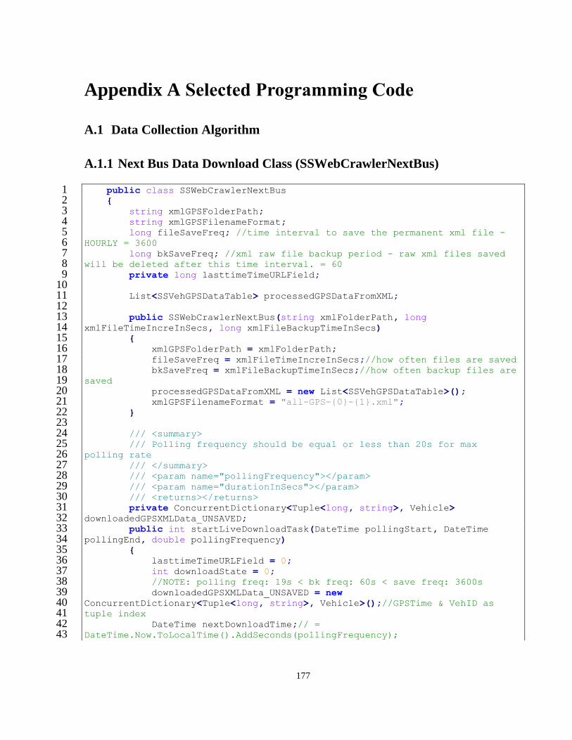
177
Appendix A Selected Programming Code
A.1 Data Collection Algorithm
A.1.1 Next Bus Data Download Class (SSWebCrawlerNextBus)
public class SSWebCrawlerNextBus 1 { 2 string xmlGPSFolderPath; 3 string xmlGPSFilenameFormat; 4 long fileSaveFreq; //time interval to save the permanent xml file - 5 HOURLY = 3600 6 long bkSaveFreq; //xml raw file backup period - raw xml files saved 7 will be deleted after this time interval. = 60 8 private long lasttimeTimeURLField; 9 10 List<SSVehGPSDataTable> processedGPSDataFromXML; 11 12 public SSWebCrawlerNextBus(string xmlFolderPath, long 13 xmlFileTimeIncreInSecs, long xmlFileBackupTimeInSecs) 14 { 15 xmlGPSFolderPath = xmlFolderPath; 16 fileSaveFreq = xmlFileTimeIncreInSecs;//how often files are saved 17 bkSaveFreq = xmlFileBackupTimeInSecs;//how often backup files are 18 saved 19 processedGPSDataFromXML = new List<SSVehGPSDataTable>(); 20 xmlGPSFilenameFormat = "all-GPS-{0}-{1}.xml"; 21 } 22 23 /// <summary> 24 /// Polling frequency should be equal or less than 20s for max 25 polling rate 26 /// </summary> 27 /// <param name="pollingFrequency"></param> 28 /// <param name="durationInSecs"></param> 29 /// <returns></returns> 30 private ConcurrentDictionary<Tuple<long, string>, Vehicle> 31 downloadedGPSXMLData_UNSAVED; 32 public int startLiveDownloadTask(DateTime pollingStart, DateTime 33 pollingEnd, double pollingFrequency) 34 { 35 lasttimeTimeURLField = 0; 36 int downloadState = 0; 37 //NOTE: polling freq: 19s < bk freq: 60s < save freq: 3600s 38 downloadedGPSXMLData_UNSAVED = new 39 ConcurrentDictionary<Tuple<long, string>, Vehicle>();//GPSTime & VehID as 40 tuple index 41 DateTime nextDownloadTime;// = 42 DateTime.Now.ToLocalTime().AddSeconds(pollingFrequency); 43

178
DateTime nextBackupTime;// = 44 DateTime.Now.ToLocalTime().AddSeconds(bkSaveFreq); 45 //DateTime nextSaveTime = 46 DateTime.Now.ToLocalTime().AddSeconds(fileSaveFreq); 47 DateTime nextSaveTime;// = 48 pollingStart.Date.AddSeconds(pollingStart.Hour * 3600 - 1 + 49 fileSaveFreq);//save on the last second of the next hour 50 long lastLogUpdatedSave = 0; 51 string bkfilename = "current-GPSXML-bk.xml"; 52 53 if (pollingStart.DateTimeToEpochTime() >= 54 DateTime.Now.ToLocalTime().DateTimeToEpochTime())//future download - put 55 thread to sleep until start - proper state 56 { 57 //return pollingStart.DateTimeToEpochTime() - 58 downloadStartTime.DateTimeToEpochTime(); 59 Thread.Sleep(Convert.ToInt32(1000 * 60 (pollingStart.DateTimeToEpochTime() - 61 DateTime.Now.ToLocalTime().DateTimeToEpochTime() - 1))); 62 nextDownloadTime = pollingStart.AddSeconds(0); 63 nextBackupTime = pollingStart.AddSeconds(0); 64 nextSaveTime = pollingStart.Date.AddSeconds(pollingStart.Hour 65 * 3600 - 1 + fileSaveFreq);//assume file save frequency is at the hour 66 } 67 else if ((pollingStart.DateTimeToEpochTime() <= 68 DateTime.Now.ToLocalTime().DateTimeToEpochTime()) && 69 (pollingEnd.DateTimeToEpochTime() > 70 DateTime.Now.ToLocalTime().DateTimeToEpochTime()))//some missing downloads - 71 start period is before download can take place 72 { 73 //polling reschedule message 74 LogUpdateEventArgs args = new LogUpdateEventArgs(); 75 args.logMessage = String.Format("NextBus Polling to Start at: 76 {0}.", 77 DateTime.Now.ToLocalTime().Date.AddSeconds(DateTime.Now.ToLocalTime().Hour * 78 3600 + fileSaveFreq).DateTimeISO8601Format()); 79 OnLogUpdate(args); 80 81 Thread.Sleep(Convert.ToInt32(1000 * (3600 - 82 (DateTime.Now.ToLocalTime().Minute * 60 + DateTime.Now.ToLocalTime().Second - 83 1)))); 84 downloadState = -1; 85 nextDownloadTime = DateTime.Now.ToLocalTime(); 86 nextBackupTime = DateTime.Now.ToLocalTime(); 87 nextSaveTime = 88 DateTime.Now.ToLocalTime().Date.AddSeconds(DateTime.Now.ToLocalTime().Hour * 89 3600 - 1 + fileSaveFreq);//assume file save frequency is at the hour 90 } 91 else 92 { 93 nextDownloadTime = new DateTime(); 94 nextBackupTime = new DateTime(); 95 nextSaveTime = new DateTime(); 96 downloadState = -2; 97
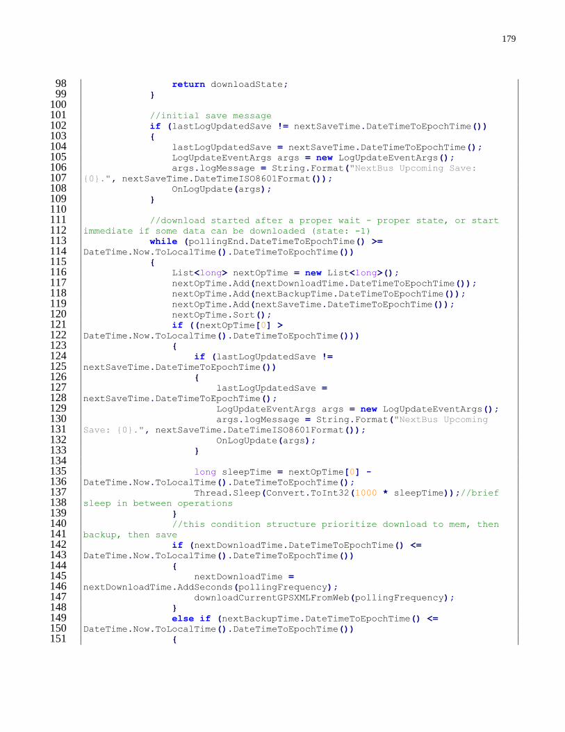
179
return downloadState; 98 } 99 100 //initial save message 101 if (lastLogUpdatedSave != nextSaveTime.DateTimeToEpochTime()) 102 { 103 lastLogUpdatedSave = nextSaveTime.DateTimeToEpochTime(); 104 LogUpdateEventArgs args = new LogUpdateEventArgs(); 105 args.logMessage = String.Format("NextBus Upcoming Save: 106 {0}.", nextSaveTime.DateTimeISO8601Format()); 107 OnLogUpdate(args); 108 } 109 110 //download started after a proper wait - proper state, or start 111 immediate if some data can be downloaded (state: -1) 112 while (pollingEnd.DateTimeToEpochTime() >= 113 DateTime.Now.ToLocalTime().DateTimeToEpochTime()) 114 { 115 List<long> nextOpTime = new List<long>(); 116 nextOpTime.Add(nextDownloadTime.DateTimeToEpochTime()); 117 nextOpTime.Add(nextBackupTime.DateTimeToEpochTime()); 118 nextOpTime.Add(nextSaveTime.DateTimeToEpochTime()); 119 nextOpTime.Sort(); 120 if ((nextOpTime[0] > 121 DateTime.Now.ToLocalTime().DateTimeToEpochTime())) 122 { 123 if (lastLogUpdatedSave != 124 nextSaveTime.DateTimeToEpochTime()) 125 { 126 lastLogUpdatedSave = 127 nextSaveTime.DateTimeToEpochTime(); 128 LogUpdateEventArgs args = new LogUpdateEventArgs(); 129 args.logMessage = String.Format("NextBus Upcoming 130 Save: {0}.", nextSaveTime.DateTimeISO8601Format()); 131 OnLogUpdate(args); 132 } 133 134 long sleepTime = nextOpTime[0] - 135 DateTime.Now.ToLocalTime().DateTimeToEpochTime(); 136 Thread.Sleep(Convert.ToInt32(1000 * sleepTime));//brief 137 sleep in between operations 138 } 139 //this condition structure prioritize download to mem, then 140 backup, then save 141 if (nextDownloadTime.DateTimeToEpochTime() <= 142 DateTime.Now.ToLocalTime().DateTimeToEpochTime()) 143 { 144 nextDownloadTime = 145 nextDownloadTime.AddSeconds(pollingFrequency); 146 downloadCurrentGPSXMLFromWeb(pollingFrequency); 147 } 148 else if (nextBackupTime.DateTimeToEpochTime() <= 149 DateTime.Now.ToLocalTime().DateTimeToEpochTime()) 150 { 151
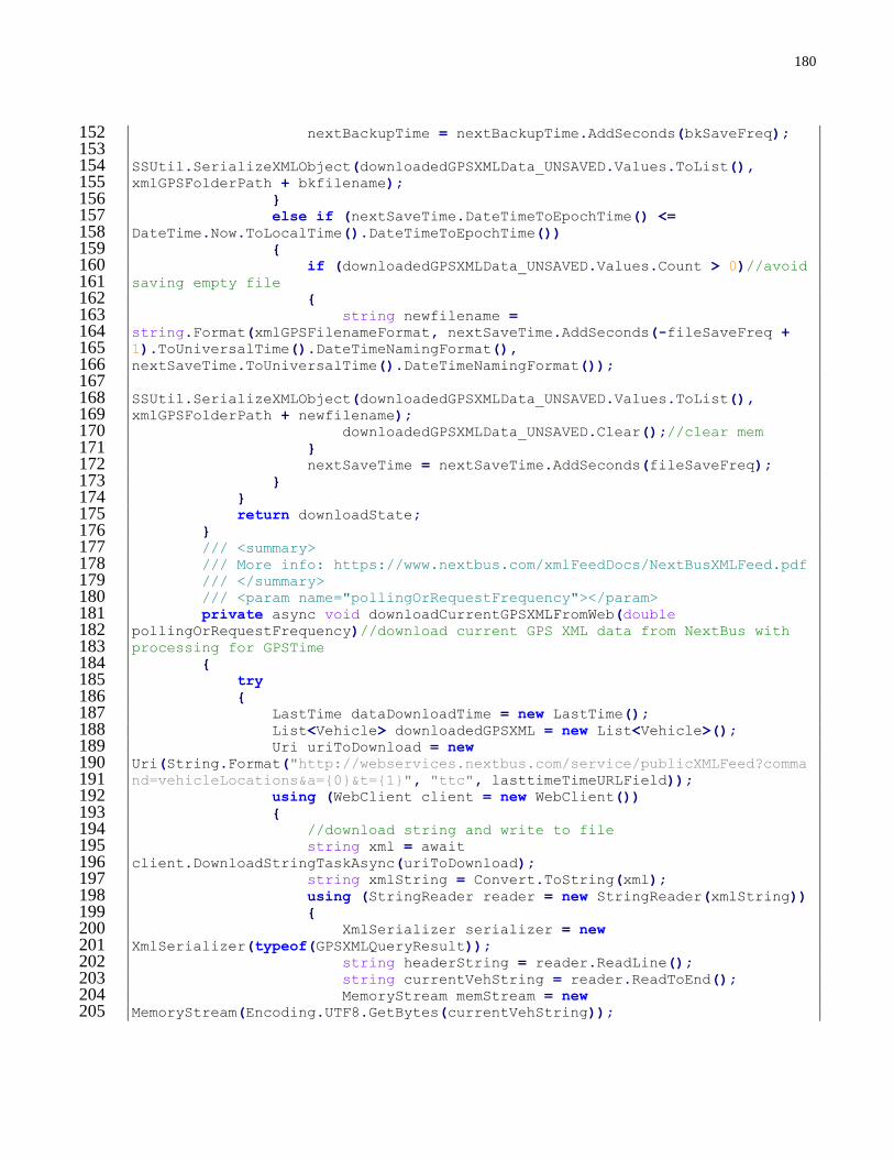
180
nextBackupTime = nextBackupTime.AddSeconds(bkSaveFreq); 152 153 SSUtil.SerializeXMLObject(downloadedGPSXMLData_UNSAVED.Values.ToList(), 154 xmlGPSFolderPath + bkfilename); 155 } 156 else if (nextSaveTime.DateTimeToEpochTime() <= 157 DateTime.Now.ToLocalTime().DateTimeToEpochTime()) 158 { 159 if (downloadedGPSXMLData_UNSAVED.Values.Count > 0)//avoid 160 saving empty file 161 { 162 string newfilename = 163 string.Format(xmlGPSFilenameFormat, nextSaveTime.AddSeconds(-fileSaveFreq + 164 1).ToUniversalTime().DateTimeNamingFormat(), 165 nextSaveTime.ToUniversalTime().DateTimeNamingFormat()); 166 167 SSUtil.SerializeXMLObject(downloadedGPSXMLData_UNSAVED.Values.ToList(), 168 xmlGPSFolderPath + newfilename); 169 downloadedGPSXMLData_UNSAVED.Clear();//clear mem 170 } 171 nextSaveTime = nextSaveTime.AddSeconds(fileSaveFreq); 172 } 173 } 174 return downloadState; 175 } 176 /// <summary> 177 /// More info: https://www.nextbus.com/xmlFeedDocs/NextBusXMLFeed.pdf 178 /// </summary> 179 /// <param name="pollingOrRequestFrequency"></param> 180 private async void downloadCurrentGPSXMLFromWeb(double 181 pollingOrRequestFrequency)//download current GPS XML data from NextBus with 182 processing for GPSTime 183 { 184 try 185 { 186 LastTime dataDownloadTime = new LastTime(); 187 List<Vehicle> downloadedGPSXML = new List<Vehicle>(); 188 Uri uriToDownload = new 189 Uri(String.Format("http://webservices.nextbus.com/service/publicXMLFeed?comma190 nd=vehicleLocations&a={0}&t={1}", "ttc", lasttimeTimeURLField)); 191 using (WebClient client = new WebClient()) 192 { 193 //download string and write to file 194 string xml = await 195 client.DownloadStringTaskAsync(uriToDownload); 196 string xmlString = Convert.ToString(xml); 197 using (StringReader reader = new StringReader(xmlString)) 198 { 199 XmlSerializer serializer = new 200 XmlSerializer(typeof(GPSXMLQueryResult)); 201 string headerString = reader.ReadLine(); 202 string currentVehString = reader.ReadToEnd(); 203 MemoryStream memStream = new 204 MemoryStream(Encoding.UTF8.GetBytes(currentVehString)); 205
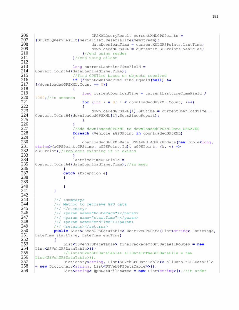
181
GPSXMLQueryResult currentXMLGPSPoints = 206 (GPSXMLQueryResult)serializer.Deserialize(memStream); 207 dataDownloadTime = currentXMLGPSPoints.LastTime; 208 downloadedGPSXML = currentXMLGPSPoints.Vehicles; 209 }//end using reader 210 }//end using cilent 211 212 long currentLasttimeTimeField = 213 Convert.ToInt64(dataDownloadTime.Time); 214 //find GPSTime based on objects received 215 if (!dataDownloadTime.Time.Equals(null) && 216 !(downloadedGPSXML.Count == 0)) 217 { 218 long currentDownloadTime = currentLasttimeTimeField / 219 1000;//in seconds 220 for (int i = 0; i < downloadedGPSXML.Count; i++) 221 { 222 downloadedGPSXML[i].GPStime = currentDownloadTime - 223 Convert.ToInt64(downloadedGPSXML[i].SecsSinceReport); 224 } 225 } 226 //Add downloadedGPSXML to downloadedGPSXMLData_UNSAVED 227 foreach (Vehicle aGPSPoint in downloadedGPSXML) 228 { 229 downloadedGPSXMLData_UNSAVED.AddOrUpdate(new Tuple<long, 230 string>(aGPSPoint.GPStime, aGPSPoint.Id), aGPSPoint, (k, v) => 231 aGPSPoint);//replaces existing if it exists 232 } 233 lasttimeTimeURLField = 234 Convert.ToInt64(dataDownloadTime.Time);//in msec 235 } 236 catch (Exception e) 237 { 238 239 } 240 } 241 242 /// <summary> 243 /// Method to retrieve GPS data 244 /// </summary> 245 /// <param name="RouteTags"></param> 246 /// <param name="startTime"></param> 247 /// <param name="endTime"></param> 248 /// <returns></returns> 249 public List<SSVehGPSDataTable> RetriveGPSData(List<string> RouteTags, 250 DateTime startTime, DateTime endTime) 251 { 252 List<SSVehGPSDataTable> finalPackageOfGPSDataAllRoutes = new 253 List<SSVehGPSDataTable>(); 254 //List<SSVehGPSDataTable> allDataInTheGPSDataFile = new 255 List<SSVehGPSDataTable>(); 256 Dictionary<string, List<SSVehGPSDataTable>> allDataInGPSDataFile 257 = new Dictionary<string, List<SSVehGPSDataTable>>(); 258 List<string> gpsDataFilenames = new List<string>();//in order 259
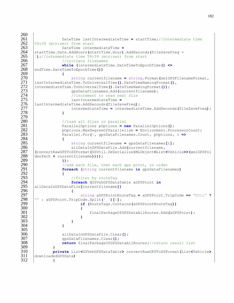
182
260 DateTime lastIntermediateTime = startTime;//intermediate time 261 59:59 (min:sec) from start 262 DateTime intermediateTime = 263 startTime.Date.AddHours(startTime.Hour).AddSeconds(fileSaveFreq - 264 1);//intermediate time 59:59 (min:sec) from start 265 //initiate filenames 266 while (intermediateTime.DateTimeToEpochTime() <= 267 endTime.DateTimeToEpochTime()) 268 { 269 string currentfilename = string.Format(xmlGPSFilenameFormat, 270 lastIntermediateTime.ToUniversalTime().DateTimeNamingFormat(), 271 intermediateTime.ToUniversalTime().DateTimeNamingFormat()); 272 gpsDataFilenames.Add(currentfilename); 273 //increment to read next file 274 lastIntermediateTime = 275 lastIntermediateTime.AddSeconds(fileSaveFreq); 276 intermediateTime = intermediateTime.AddSeconds(fileSaveFreq); 277 } 278 279 //load all files in parallel 280 ParallelOptions pOptions = new ParallelOptions(); 281 pOptions.MaxDegreeOfParallelism = Environment.ProcessorCount; 282 Parallel.For(0, gpsDataFilenames.Count, pOptions, i => 283 { 284 string currentfilename = gpsDataFilenames[i]; 285 allDataInGPSDataFile.Add(currentfilename, 286 (convertRawGPSToSSFormat(SSUtil.DeSerializeXMLObject<List<Vehicle>>(xmlGPSFol287 derPath + currentfilename)))); 288 }); 289 //add each file, then each gps point, in order 290 foreach (string currentfilename in gpsDataFilenames) 291 { 292 //filter by routeTag 293 foreach (SSVehGPSDataTable aGPSPoint in 294 allDataInGPSDataFile[currentfilename]) 295 { 296 string aGPSPointRouteTag = aGPSPoint.TripCode == "NULL" ? 297 "" : aGPSPoint.TripCode.Split('_')[0]; 298 if (RouteTags.Contains(aGPSPointRouteTag)) 299 { 300 finalPackageOfGPSDataAllRoutes.Add(aGPSPoint); 301 } 302 } 303 } 304 305 allDataInGPSDataFile.Clear(); 306 gpsDataFilenames.Clear(); 307 return finalPackageOfGPSDataAllRoutes;//return result list 308 } 309 private List<SSVehGPSDataTable> convertRawGPSToSSFormat(List<Vehicle> 310 downloadedGPSData) 311 { 312
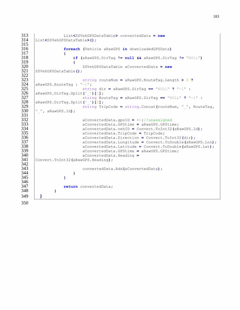
183
List<SSVehGPSDataTable> convertedData = new 313 List<SSVehGPSDataTable>(); 314 315 foreach (Vehicle aRawGPS in downloadedGPSData) 316 { 317 if (aRawGPS.DirTag != null && aRawGPS.DirTag != "NULL") 318 { 319 SSVehGPSDataTable aConvertedData = new 320 SSVehGPSDataTable(); 321 322 string routeNum = aRawGPS.RouteTag.Length > 0 ? 323 aRawGPS.RouteTag : "-1"; 324 string dir = aRawGPS.DirTag == "NULL" ? "-1" : 325 aRawGPS.DirTag.Split('_')[1]; 326 string RouteTag = aRawGPS.DirTag == "NULL" ? "-1" : 327 aRawGPS.DirTag.Split('_')[2]; 328 string TripCode = string.Concat(routeNum, "_", RouteTag, 329 "_", aRawGPS.Id); 330 331 aConvertedData.gpsID = -1;//unassigned 332 aConvertedData.GPStime = aRawGPS.GPStime; 333 aConvertedData.vehID = Convert.ToInt32(aRawGPS.Id); 334 aConvertedData.TripCode = TripCode; 335 aConvertedData.Direction = Convert.ToInt32(dir); 336 aConvertedData.Longitude = Convert.ToDouble(aRawGPS.Lon); 337 aConvertedData.Latitude = Convert.ToDouble(aRawGPS.Lat); 338 aConvertedData.GPStime = aRawGPS.GPStime; 339 aConvertedData.Heading = 340 Convert.ToInt32(aRawGPS.Heading); 341 342 convertedData.Add(aConvertedData); 343 } 344 } 345 346 return convertedData; 347 } 348
} 349
350
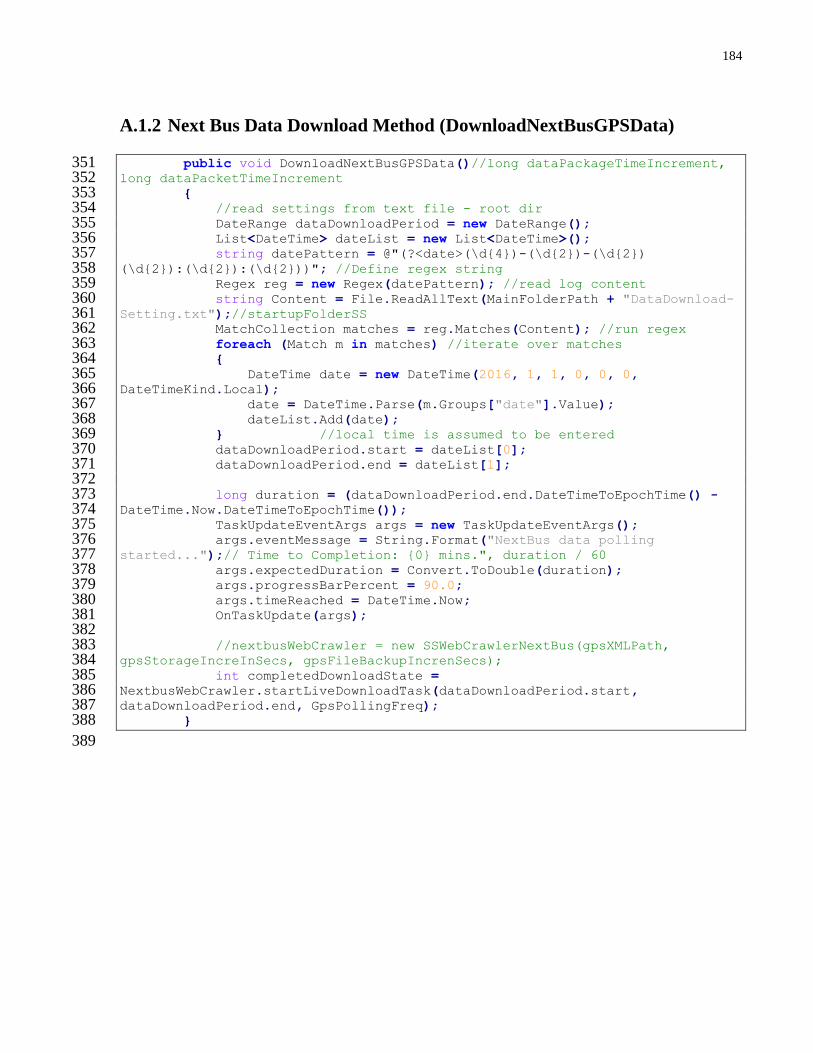
184
A.1.2 Next Bus Data Download Method (DownloadNextBusGPSData)
public void DownloadNextBusGPSData()//long dataPackageTimeIncrement, 351 long dataPacketTimeIncrement 352 { 353 //read settings from text file - root dir 354 DateRange dataDownloadPeriod = new DateRange(); 355 List<DateTime> dateList = new List<DateTime>(); 356 string datePattern = @"(?<date>(\d{4})-(\d{2})-(\d{2}) 357 (\d{2}):(\d{2}):(\d{2}))"; //Define regex string 358 Regex reg = new Regex(datePattern); //read log content 359 string Content = File.ReadAllText(MainFolderPath + "DataDownload-360 Setting.txt");//startupFolderSS 361 MatchCollection matches = reg.Matches(Content); //run regex 362 foreach (Match m in matches) //iterate over matches 363 { 364 DateTime date = new DateTime(2016, 1, 1, 0, 0, 0, 365 DateTimeKind.Local); 366 date = DateTime.Parse(m.Groups["date"].Value); 367 dateList.Add(date); 368 } //local time is assumed to be entered 369 dataDownloadPeriod.start = dateList[0]; 370 dataDownloadPeriod.end = dateList[1]; 371 372 long duration = (dataDownloadPeriod.end.DateTimeToEpochTime() - 373 DateTime.Now.DateTimeToEpochTime()); 374 TaskUpdateEventArgs args = new TaskUpdateEventArgs(); 375 args.eventMessage = String.Format("NextBus data polling 376 started...");// Time to Completion: {0} mins.", duration / 60 377 args.expectedDuration = Convert.ToDouble(duration); 378 args.progressBarPercent = 90.0; 379 args.timeReached = DateTime.Now; 380 OnTaskUpdate(args); 381 382 //nextbusWebCrawler = new SSWebCrawlerNextBus(gpsXMLPath, 383 gpsStorageIncreInSecs, gpsFileBackupIncrenSecs); 384 int completedDownloadState = 385 NextbusWebCrawler.startLiveDownloadTask(dataDownloadPeriod.start, 386 dataDownloadPeriod.end, GpsPollingFreq); 387 } 388
389
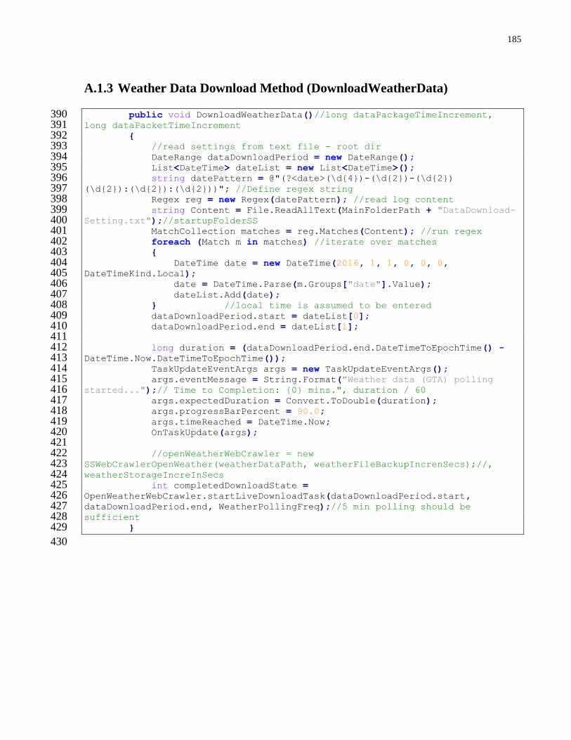
185
A.1.3 Weather Data Download Method (DownloadWeatherData)
public void DownloadWeatherData()//long dataPackageTimeIncrement, 390 long dataPacketTimeIncrement 391 { 392 //read settings from text file - root dir 393 DateRange dataDownloadPeriod = new DateRange(); 394 List<DateTime> dateList = new List<DateTime>(); 395 string datePattern = @"(?<date>(\d{4})-(\d{2})-(\d{2}) 396 (\d{2}):(\d{2}):(\d{2}))"; //Define regex string 397 Regex reg = new Regex(datePattern); //read log content 398 string Content = File.ReadAllText(MainFolderPath + "DataDownload-399 Setting.txt");//startupFolderSS 400 MatchCollection matches = reg.Matches(Content); //run regex 401 foreach (Match m in matches) //iterate over matches 402 { 403 DateTime date = new DateTime(2016, 1, 1, 0, 0, 0, 404 DateTimeKind.Local); 405 date = DateTime.Parse(m.Groups["date"].Value); 406 dateList.Add(date); 407 } //local time is assumed to be entered 408 dataDownloadPeriod.start = dateList[0]; 409 dataDownloadPeriod.end = dateList[1]; 410 411 long duration = (dataDownloadPeriod.end.DateTimeToEpochTime() - 412 DateTime.Now.DateTimeToEpochTime()); 413 TaskUpdateEventArgs args = new TaskUpdateEventArgs(); 414 args.eventMessage = String.Format("Weather data (GTA) polling 415 started...");// Time to Completion: {0} mins.", duration / 60 416 args.expectedDuration = Convert.ToDouble(duration); 417 args.progressBarPercent = 90.0; 418 args.timeReached = DateTime.Now; 419 OnTaskUpdate(args); 420 421 //openWeatherWebCrawler = new 422 SSWebCrawlerOpenWeather(weatherDataPath, weatherFileBackupIncrenSecs);//, 423 weatherStorageIncreInSecs 424 int completedDownloadState = 425 OpenWeatherWebCrawler.startLiveDownloadTask(dataDownloadPeriod.start, 426 dataDownloadPeriod.end, WeatherPollingFreq);//5 min polling should be 427 sufficient 428 } 429
430
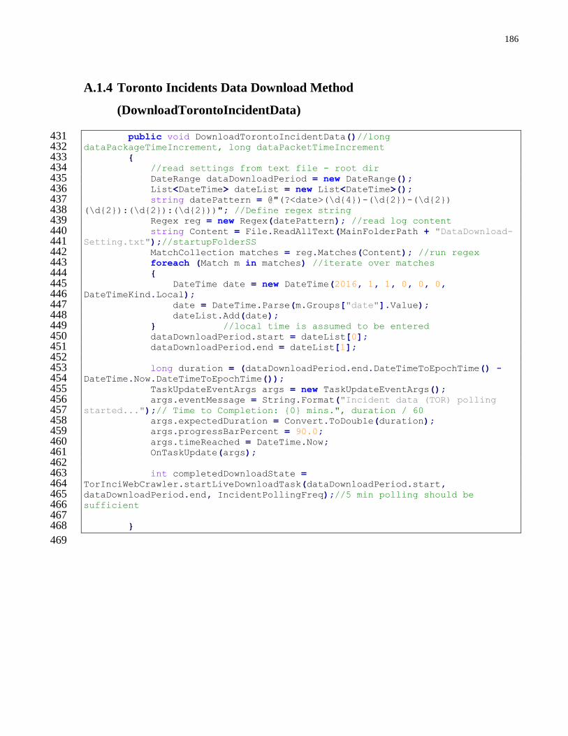
186
A.1.4 Toronto Incidents Data Download Method
(DownloadTorontoIncidentData)
public void DownloadTorontoIncidentData()//long 431 dataPackageTimeIncrement, long dataPacketTimeIncrement 432 { 433 //read settings from text file - root dir 434 DateRange dataDownloadPeriod = new DateRange(); 435 List<DateTime> dateList = new List<DateTime>(); 436 string datePattern = @"(?<date>(\d{4})-(\d{2})-(\d{2}) 437 (\d{2}):(\d{2}):(\d{2}))"; //Define regex string 438 Regex reg = new Regex(datePattern); //read log content 439 string Content = File.ReadAllText(MainFolderPath + "DataDownload-440 Setting.txt");//startupFolderSS 441 MatchCollection matches = reg.Matches(Content); //run regex 442 foreach (Match m in matches) //iterate over matches 443 { 444 DateTime date = new DateTime(2016, 1, 1, 0, 0, 0, 445 DateTimeKind.Local); 446 date = DateTime.Parse(m.Groups["date"].Value); 447 dateList.Add(date); 448 } //local time is assumed to be entered 449 dataDownloadPeriod.start = dateList[0]; 450 dataDownloadPeriod.end = dateList[1]; 451 452 long duration = (dataDownloadPeriod.end.DateTimeToEpochTime() - 453 DateTime.Now.DateTimeToEpochTime()); 454 TaskUpdateEventArgs args = new TaskUpdateEventArgs(); 455 args.eventMessage = String.Format("Incident data (TOR) polling 456 started...");// Time to Completion: {0} mins.", duration / 60 457 args.expectedDuration = Convert.ToDouble(duration); 458 args.progressBarPercent = 90.0; 459 args.timeReached = DateTime.Now; 460 OnTaskUpdate(args); 461 462 int completedDownloadState = 463 TorInciWebCrawler.startLiveDownloadTask(dataDownloadPeriod.start, 464 dataDownloadPeriod.end, IncidentPollingFreq);//5 min polling should be 465 sufficient 466 467 } 468
469

187
A.1.5 Offline Data Loading Method (LoadDataFromOfflineFile)
public void LoadDataFromOfflineFiles(bool includeIncidentData, bool 470 includeWeatherData) 471 { 472 bool saveChangesToDb = true; 473 UpdateAndLoadGPSDbDataFromFiles(saveChangesToDb);//update gps 474 database and load new gps points to data object 475 //1. Load GTFS and AVL data 476 if (!File.Exists(DbFile_GTFS) || StartNewGTFSdbFiles) 477 { 478 GTFSDatabase = new 479 GTFSConvertSSim(Path.GetDirectoryName(DbFile_GTFS), 480 Path.GetFileName(DbFile_GTFS)); 481 482 GTFSDatabase.btn_Convert_and_Save_Click(); 483 GTFSDatabase.generateSQLiteDB_SSim(); 484 } 485 LoadGTFSReferenceData();// read GTFS data for network 486 initialization 487 InitializeGPSTripDB(false);//process new GPS points, let changes 488 be saved after with incident and weather 489 490 //2. Load and process Incident and Weather Data 491 if (includeIncidentData) 492 { 493 //load Incident Data 494 UpdateDbIncidentDataFromFiles(); 495 RdIncidentsTable = GetTorInciDataFromDB(); 496 //Compute incident value for newly loaded GPS points 497 } 498 if (includeWeatherData) 499 { 500 //load Weather Data 501 UpdateDbWeatherDataFromFiles(); 502 WeatherTable = GetWeatherDataFromDB(); 503 //Compute weather value for newly loaded GPS points 504 } 505 SSFileReaderTorINTXN intxnReader = new 506 SSFileReaderTorINTXN(TrafficSignalFile, TrafficIntnxVolFile, 507 TrafficPedCrossFile, TrafficFlasingBeaconFile); 508 IntxnSignalTable = intxnReader.getCombinedIntxnData(); 509 510 SaveSimulatorDbChanges(false); 511 UpdateGUI_StatusBox("Source data loaded...", 100.0, 0.0); 512 } 513 514
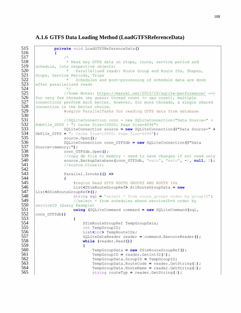
188
A.1.6 GTFS Data Loading Method (LoadGTFSReferenceData)
private void LoadGTFSReferenceData() 515 { 516 /* 517 * Read key GTFS data on stops, route, service period and 518 schedule, into respective objects: 519 * Parallelized reads: Route Group and Route IDs, Shapes, 520 Stops, Service Periods, Trips 521 * Schedules and post-processing of schedule data are done 522 after parallelized reads 523 */ 524 //Some Notes: https://manski.net/2012/10/sqlite-performance/ ==> 525 for very few threads (my guess: thread count <= cpu count), multiple 526 connections perform much better. However, for more threads, a single shared 527 connection is the better choice. 528 #region ParallelTasks for reading GTFS data from database 529 530 //SQLiteConnection conn = new SQLiteConnection("Data Source=" + 531 @dbFile_GTFS + "; Cache Size=10000; Page Size=4096") 532 SQLiteConnection source = new SQLiteConnection(@"Data Source=" + 533 DbFile_GTFS + "; Cache Size=10000; Page Size=4096"); 534 source.Open(); 535 SQLiteConnection conn_GTFSdb = new SQLiteConnection(@"Data 536 Source=:memory:"); 537 conn_GTFSdb.Open(); 538 //copy db file to memory - need to save changes if not read only 539 source.BackupDatabase(conn_GTFSdb, "main", "main", -1, null, 0); 540 //source.Close(); 541 542 Parallel.Invoke(() => 543 { 544 #region Read GTFS ROUTE GROUPS AND ROUTE IDs 545 List<SSimRouteGroupRef> AllRouteGroupData = new 546 List<SSimRouteGroupRef>(); 547 string sql = "select * from route_groups order by groupID"; 548 //select * from schedules where serviceID=4 order by 549 serviceID (Query Example) 550 using (SQLiteCommand command = new SQLiteCommand(sql, 551 conn_GTFSdb)) 552 { 553 SSimRouteGroupRef TempGroupData; 554 int TempGroupID; 555 List<int> TempRouteIDs; 556 SQLiteDataReader reader = command.ExecuteReader(); 557 while (reader.Read()) 558 { 559 TempGroupData = new SSimRouteGroupRef(); 560 TempGroupID = reader.GetInt32(0); 561 TempGroupData.GroupID = TempGroupID; 562 TempGroupData.RouteCode = reader.GetString(1); 563 TempGroupData.RouteName = reader.GetString(2); 564 string routeTyp = reader.GetString(3); 565

189
TempGroupData.RouteType = 566 (routeTyp.Equals("surface_fixed") ? routeType.surface_fixed : 567 (routeTyp.Equals("underground") ? routeType.underground : 568 (routeTyp.Equals("surface_separated") ? routeType.surface_separated : 569 (routeTyp.Equals("surface_variable") ? routeType.surface_variable : 570 (routeTyp.Equals("aerial") ? routeType.aerial : routeType.aerial))))); 571 572 TempGroupData.AgencyID = reader.GetInt32(4); 573 574 string sql2_routesInGroup = "select * from routes 575 where groupID=" + TempGroupID + " order by routeID"; 576 using (SQLiteCommand command_route = new 577 SQLiteCommand(sql2_routesInGroup, conn_GTFSdb)) 578 { 579 SQLiteDataReader reader_route = 580 command_route.ExecuteReader(); 581 TempRouteIDs = new List<int>(); 582 ConcurrentDictionary<int, SSimRouteRef> 583 TempRouteInfo = new ConcurrentDictionary<int, SSimRouteRef>();//routeInfo by 584 routeID - Temp 585 586 while (reader_route.Read()) 587 { 588 SSimRouteRef TempSingleRouteInfo = new 589 SSimRouteRef(); 590 TempRouteIDs.Add(reader_route.GetInt32(0)); 591 string name = 592 reader_route.GetString(2).Replace(" - ", "^"); 593 string[] nameArray = name.Split('^'); 594 TempSingleRouteInfo.RouteTag = 595 nameArray[1].Split(' ').First().ToUpper(); 596 TempSingleRouteInfo.DirTag = 597 Convert.ToInt32(name.Split('^').Last().Split(' ').Last()); 598 TempSingleRouteInfo.Include = false; 599 //default to exclude the route from analysis 600 TempSingleRouteInfo.Name = string.Format("{0} 601 - {1}B", nameArray[1], nameArray[0][0]);//i.e.: 94A WELLESLEY TOWARDS 602 OSSINGTON STATION - WB 603 604 605 TempRouteInfo.GetOrAdd(Convert.ToInt32(reader_route.GetInt32(0)), 606 TempSingleRouteInfo); 607 TempSingleRouteInfo = null; 608 } 609 TempGroupData.RouteIDs = TempRouteIDs; 610 TempGroupData.RouteInfo = TempRouteInfo; 611 TempGroupData.serviceAvailByServiceP = new 612 ConcurrentDictionary<int, bool>(); 613 TempGroupData.mainRouteIDDir0ByServiceP = new 614 ConcurrentDictionary<int, int>(); 615 TempGroupData.mainRouteIDDir1ByServiceP = new 616 ConcurrentDictionary<int, int>(); 617 TempGroupData.subRouteIDDir0 = new 618 List<Tuple<int, string, int>>(); 619
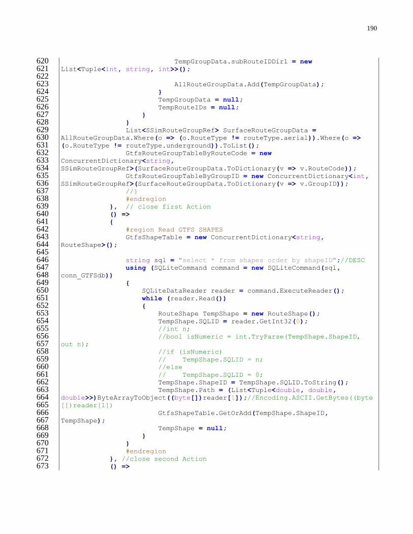
190
TempGroupData.subRouteIDDir1 = new 620 List<Tuple<int, string, int>>(); 621 622 AllRouteGroupData.Add(TempGroupData); 623 } 624 TempGroupData = null; 625 TempRouteIDs = null; 626 } 627 } 628 List<SSimRouteGroupRef> SurfaceRouteGroupData = 629 AllRouteGroupData.Where(o => (o.RouteType != routeType.aerial)).Where(o => 630 (o.RouteType != routeType.underground)).ToList(); 631 GtfsRouteGroupTableByRouteCode = new 632 ConcurrentDictionary<string, 633 SSimRouteGroupRef>(SurfaceRouteGroupData.ToDictionary(v => v.RouteCode)); 634 GtfsRouteGroupTableByGroupID = new ConcurrentDictionary<int, 635 SSimRouteGroupRef>(SurfaceRouteGroupData.ToDictionary(v => v.GroupID)); 636 //} 637 #endregion 638 }, // close first Action 639 () => 640 { 641 #region Read GTFS SHAPES 642 GtfsShapeTable = new ConcurrentDictionary<string, 643 RouteShape>(); 644 645 string sql = "select * from shapes order by shapeID";//DESC 646 using (SQLiteCommand command = new SQLiteCommand(sql, 647 conn_GTFSdb)) 648 { 649 SQLiteDataReader reader = command.ExecuteReader(); 650 while (reader.Read()) 651 { 652 RouteShape TempShape = new RouteShape(); 653 TempShape.SQLID = reader.GetInt32(0); 654 //int n; 655 //bool isNumeric = int.TryParse(TempShape.ShapeID, 656 out n); 657 //if (isNumeric) 658 // TempShape.SQLID = n; 659 //else 660 // TempShape.SQLID = 0; 661 TempShape.ShapeID = TempShape.SQLID.ToString(); 662 TempShape.Path = (List<Tuple<double, double, 663 double>>)ByteArrayToObject((byte[])reader[1]);//Encoding.ASCII.GetBytes((byte664 [])reader[1]) 665 GtfsShapeTable.GetOrAdd(TempShape.ShapeID, 666 TempShape); 667 TempShape = null; 668 } 669 } 670 #endregion 671 }, //close second Action 672 () => 673

191
{ 674 #region Read GTFS STOPS 675 GtfsStopTable = new ConcurrentDictionary<int, SSimStopRef>(); 676 //contains all stop reference, with GPS and stop types. TempStopID as 677 reference. 678 string sql = "select * from stops order by stopID"; 679 using (SQLiteCommand command = new SQLiteCommand(sql, 680 conn_GTFSdb)) 681 { 682 SSimStopRef TempStopData; 683 int TempStopID; 684 SQLiteDataReader reader = command.ExecuteReader(); 685 while (reader.Read()) 686 { 687 TempStopData = new SSimStopRef(); 688 TempStopID = reader.GetInt32(0); 689 TempStopData.StopID = TempStopID; 690 TempStopData.StopCode = reader.GetString(1); 691 TempStopData.Longitude = reader.GetDouble(2); 692 TempStopData.Latitude = reader.GetDouble(3); 693 string stopTyp = reader.GetString(4); 694 TempStopData.StopType = 695 (stopTyp.Equals("platform_bus") ? stopType.platform_bus : 696 (stopTyp.Equals("platform_train") ? 697 stopType.platform_train : 698 (stopTyp.Equals("stop") ? stopType.stop : 699 (stopTyp.Equals("doorway") ? stopType.doorway 700 : 701 (stopTyp.Equals("vehicle_yard") ? 702 stopType.vehicle_yard : 703 (stopTyp.Equals("subway_stop") ? 704 stopType.subway_stop : 705 (stopTyp.Equals("timing_stop") ? 706 stopType.timing_stop : stopType.timing_stop)))))));//subway_stop: modified 707 stop type for subway transfer stations 708 TempStopData.StopName = reader.GetString(5); 709 710 //double check to make sure subway_stop is correctly 711 assigned 712 if ((TempStopData.StopName.Contains("STATION") && 713 TempStopData.StopName.Contains(" AT ") && 714 !TempStopData.StopName.Contains("STATION LOOP")) || 715 (TempStopData.StopName.Contains("STATION)"))) 716 { 717 TempStopData.StopType = stopType.subway_stop; 718 //newStop.StopName += " - SUBWAY STOP";//Not 719 needed 720 } 721 722 string connectingstopstring = reader.GetString(6); 723 string[] connectingstopstringarray; 724 int[] connectingstopInt; 725 if (connectingstopstring != "none") 726 { 727

192
connectingstopstringarray = 728 connectingstopstring.Split(' '); 729 connectingstopInt = 730 Array.ConvertAll(connectingstopstringarray, int.Parse); 731 TempStopData.ConnectingStopIDs = 732 connectingstopInt.ToList(); 733 } 734 TempStopData.scheduledStopTimesByServiceID = 735 (Dictionary<int, List<TimeSpan>>)ByteArrayToObject((byte[])reader[7]); 736 737 //string stopTimesString = reader.GetString(7); 738 //Array.ConvertAll(stopTimesString.Split(' '), 739 TimeSpan.Parse).ToList(); 740 741 GtfsStopTable.GetOrAdd(TempStopID, 742 TempStopData);//uses stopId as index 743 TempStopData = null; 744 } 745 } 746 747 AssignDefaultDataProcessingSettings();//get all stops that 748 needs to have exceptions 749 750 #endregion 751 }, //close third Action 752 () => 753 { 754 #region read GTFS SERVICE PERIODS 755 GtfsServicePeriodTable = new ConcurrentDictionary<int, 756 SSimServicePeriodsRef>();//contains list of service period types and 757 respective agency. Service ID as reference. 758 string sql = "select * from servicePeriods order by 759 serviceID"; 760 using (SQLiteCommand command = new SQLiteCommand(sql, 761 conn_GTFSdb)) 762 { 763 SSimServicePeriodsRef TempServiceData; 764 int TempServiceID; 765 SQLiteDataReader reader = command.ExecuteReader(); 766 while (reader.Read()) 767 { 768 TempServiceData = new SSimServicePeriodsRef(); 769 TempServiceID = reader.GetInt32(0); 770 TempServiceData.ServiceID = TempServiceID; 771 string dayTyp = reader.GetString(1); 772 TempServiceData.TypeOfDay = (dayTyp.Equals("weekday") 773 ? dayType.weekday : (dayTyp.Equals("saturday") ? dayType.saturday : 774 (dayTyp.Equals("sunday") ? dayType.sunday : (dayTyp.Equals("special") ? 775 dayType.special : dayType.special))));//second special day not handled here 776 //TempServiceData.agencyID = 777 Convert.ToInt32(reader[2]); 778 GtfsServicePeriodTable.GetOrAdd(TempServiceID, 779 TempServiceData); 780

193
781 //servicePeriodTable.Add(Convert.ToInt32(TempServiceData.typeOfDay), 782 TempServiceData);//duplicated special daytype 783 TempServiceData = null; 784 } 785 } 786 #endregion 787 }, //close forth Action 788 () => 789 { 790 #region Read GTFS TRIPS - need to be run before schedule 791 //ConcurrentDictionary<int, SSimGTFSTripRef> 792 GtfsTripTable = new ConcurrentDictionary<int, 793 SSimGTFSTripRef>();//contains list of service period types and respective 794 agency. Service ID as reference. 795 GtfsTripIDByScheduleID = new Dictionary<int, 796 List<int>>();//use for post-processing schedule table 797 string sql = "select * from trips order by TripID";//DESC 798 using (SQLiteCommand command = new SQLiteCommand(sql, 799 conn_GTFSdb)) 800 { 801 SQLiteDataReader reader = command.ExecuteReader(); 802 while (reader.Read()) 803 { 804 SSimGTFSTripRef TempTrip = new SSimGTFSTripRef(); 805 TempTrip.gtfsTripID = reader.GetInt32(0); 806 TempTrip.ScheduleID = reader.GetInt32(1); 807 TempTrip.BlockID = reader.GetInt32(2); 808 //TempTrip.shapeID = Convert.ToInt32(reader[3]); 809 TempTrip.StartStopID = reader.GetInt32(4); 810 TempTrip.EndStopID = reader.GetInt32(5); 811 long TempTicks = reader.GetInt64(6); 812 TimeSpan TempTimeSpan = 813 TimeSpan.FromTicks(TempTicks); 814 TempTrip.ReleaseTime = TempTimeSpan; 815 string stopTimesString = reader.GetString(7); 816 TempTrip.StopTimes = 817 Array.ConvertAll(stopTimesString.Split(' '), TimeSpan.Parse).ToList(); 818 //TempTrip.tripScheduleInfo = 819 gtfsScheduleTable[TempTrip.scheduleID]; 820 821 GtfsTripTable.GetOrAdd(TempTrip.gtfsTripID, 822 TempTrip); 823 if 824 (GtfsTripIDByScheduleID.ContainsKey(TempTrip.ScheduleID)) 825 { 826 827 GtfsTripIDByScheduleID[TempTrip.ScheduleID].Add(TempTrip.gtfsTripID); 828 } 829 else 830 { 831 List<int> TempTripIDs = new List<int>(); 832 TempTripIDs.Add(TempTrip.gtfsTripID); 833

194
GtfsTripIDByScheduleID.Add(TempTrip.ScheduleID, 834 TempTripIDs); 835 } 836 837 TempTrip = null; 838 } 839 } 840 #endregion 841 } //close fifth Action, 842 ); //close parallel.invoke 843 #endregion 844 845 #region Read GTFS SCHEDULES with stop distances 846 //Service Period ID as index for the masterScheduleTable - to get 847 the SSimRouteScheduleRef 848 //ConcurrentDictionary<int, SSimScheduleRef> 849 scheduleTableByScheduleID = new ConcurrentDictionary<int, 850 SSimScheduleRef>();//index by schedule id 851 GtfsScheduleTable = new ConcurrentDictionary<int, 852 SSimScheduleRef>();//index by schedule id 853 GtfsScheduleIDLookupTable = new ConcurrentDictionary<int, 854 SSimServiceScheduleRef>();//construct 855 foreach (var servicep in GtfsServicePeriodTable) 856 { 857 //Dictionary<int, int> TempRouteIDbyScheduleID = new 858 Dictionary<int, int>(); 859 int currentServiceID = servicep.Value.ServiceID; 860 861 SSimServiceScheduleRef TempRouteScheduleData = new 862 SSimServiceScheduleRef(); 863 ConcurrentDictionary<int, int> TempScheduleIDByRouteID = new 864 ConcurrentDictionary<int, int>(); 865 866 string sql = "select * from schedules where serviceID=" + 867 servicep.Value.ServiceID + " order by serviceID DESC"; 868 using (SQLiteCommand command = new SQLiteCommand(sql, 869 conn_GTFSdb)) 870 { 871 SQLiteDataReader reader = command.ExecuteReader(); 872 while (reader.Read()) 873 { 874 SSimScheduleRef TempSingleScheduleData = new 875 SSimScheduleRef(); 876 int TempScheduleID = reader.GetInt32(0); 877 int TempServiceID = reader.GetInt32(1); 878 int TempRouteID = reader.GetInt32(2); 879 int TempGroupID = reader.GetInt32(3); 880 string routestopstring = reader.GetString(4); 881 string routestopdiststring = reader.GetString(5); 882 string TempShapeID = "" + reader.GetInt32(6); 883 884 //TempRouteIDbyScheduleID.Add(TempScheduleID, 885 TempRouteID); 886 TempSingleScheduleData.GroupID = TempGroupID; 887
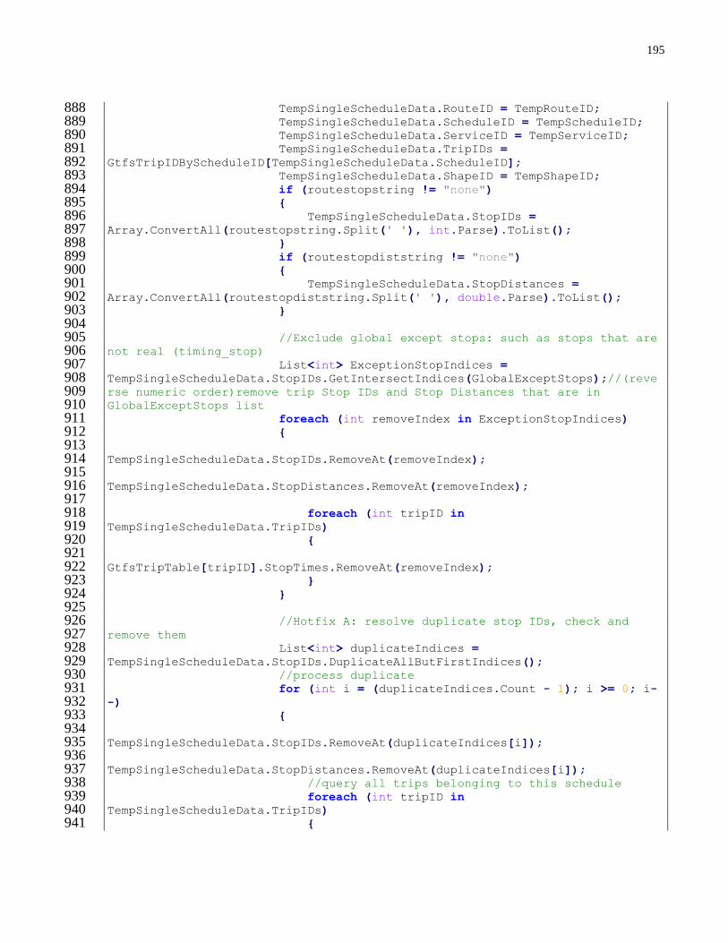
195
TempSingleScheduleData.RouteID = TempRouteID; 888 TempSingleScheduleData.ScheduleID = TempScheduleID; 889 TempSingleScheduleData.ServiceID = TempServiceID; 890 TempSingleScheduleData.TripIDs = 891 GtfsTripIDByScheduleID[TempSingleScheduleData.ScheduleID]; 892 TempSingleScheduleData.ShapeID = TempShapeID; 893 if (routestopstring != "none") 894 { 895 TempSingleScheduleData.StopIDs = 896 Array.ConvertAll(routestopstring.Split(' '), int.Parse).ToList(); 897 } 898 if (routestopdiststring != "none") 899 { 900 TempSingleScheduleData.StopDistances = 901 Array.ConvertAll(routestopdiststring.Split(' '), double.Parse).ToList(); 902 } 903 904 //Exclude global except stops: such as stops that are 905 not real (timing_stop) 906 List<int> ExceptionStopIndices = 907 TempSingleScheduleData.StopIDs.GetIntersectIndices(GlobalExceptStops);//(reve908 rse numeric order)remove trip Stop IDs and Stop Distances that are in 909 GlobalExceptStops list 910 foreach (int removeIndex in ExceptionStopIndices) 911 { 912 913 TempSingleScheduleData.StopIDs.RemoveAt(removeIndex); 914 915 TempSingleScheduleData.StopDistances.RemoveAt(removeIndex); 916 917 foreach (int tripID in 918 TempSingleScheduleData.TripIDs) 919 { 920 921 GtfsTripTable[tripID].StopTimes.RemoveAt(removeIndex); 922 } 923 } 924 925 //Hotfix A: resolve duplicate stop IDs, check and 926 remove them 927 List<int> duplicateIndices = 928 TempSingleScheduleData.StopIDs.DuplicateAllButFirstIndices(); 929 //process duplicate 930 for (int i = (duplicateIndices.Count - 1); i >= 0; i-931 -) 932 { 933 934 TempSingleScheduleData.StopIDs.RemoveAt(duplicateIndices[i]); 935 936 TempSingleScheduleData.StopDistances.RemoveAt(duplicateIndices[i]); 937 //query all trips belonging to this schedule 938 foreach (int tripID in 939 TempSingleScheduleData.TripIDs) 940 { 941
196
942 GtfsTripTable[tripID].StopTimes.RemoveAt(duplicateIndices[i]); 943 } 944 945 } 946 947 TempScheduleIDByRouteID.GetOrAdd(TempRouteID, 948 TempScheduleID);//a copy for master schedule table - by service period then 949 route id 950 GtfsScheduleTable.GetOrAdd(TempScheduleID, 951 TempSingleScheduleData);//simple schedule table lookup 952 TempSingleScheduleData = null; 953 } 954 } 955 TempRouteScheduleData.ServiceID = currentServiceID; 956 TempRouteScheduleData.ScheduleIDByRouteID = 957 TempScheduleIDByRouteID; 958 //TempRouteScheduleData.routeIDbyScheduleID = 959 TempRouteIDbyScheduleID; 960 GtfsScheduleIDLookupTable.GetOrAdd(currentServiceID, 961 TempRouteScheduleData); 962 963 TempRouteScheduleData = null; 964 //TempRouteIDbyScheduleID = null; 965 TempScheduleIDByRouteID = null; 966 //SSimSingleScheduleRef TempRouteScheduleData22 = 967 masterScheduleTable[1].routeSchedule[4];//test if index 4 is route 4 or 5th 968 position-->YES 969 } 970 971 //Remove trips that don't exist in schedule and route group 972 SSimGTFSTripRef anotherTempTripRef; 973 List<int> tripIDsToBeRemoved = new List<int>(); 974 foreach (int tripID in GtfsTripTable.Keys) 975 { 976 int scheduleID = GtfsTripTable[tripID].ScheduleID; 977 if (!GtfsScheduleTable.ContainsKey(scheduleID)) 978 { 979 tripIDsToBeRemoved.Add(tripID); 980 } 981 else 982 { 983 int groupID = GtfsScheduleTable[scheduleID].GroupID; 984 if (!GtfsRouteGroupTableByGroupID.ContainsKey(groupID)) 985 { 986 tripIDsToBeRemoved.Add(tripID); 987 } 988 } 989 } 990 foreach (int tripIDToRemove in tripIDsToBeRemoved) 991 { 992 GtfsTripTable.TryRemove(tripIDToRemove, out 993 anotherTempTripRef); 994 } 995
197
996 //Remove zero size schedules and trips 997 List<int> scheduleIDsToBeRemoved = new List<int>(); 998 foreach (int scheduleID in GtfsScheduleTable.Keys) 999 { 1000 if (GtfsScheduleTable[scheduleID].StopIDs.Count == 0) 1001 { 1002 scheduleIDsToBeRemoved.Add(scheduleID); 1003 } 1004 } 1005 SSimScheduleRef tempScheduleRef; 1006 SSimRouteRef tempRouteRef; 1007 SSimGTFSTripRef tempTripRef; 1008 foreach (int scheduleIDToRemove in scheduleIDsToBeRemoved) 1009 { 1010 foreach (int tripIDToRemove in 1011 GtfsScheduleTable[scheduleIDToRemove].TripIDs) 1012 { 1013 GtfsTripTable.TryRemove(tripIDToRemove, out tempTripRef); 1014 } 1015 int groupID = GtfsScheduleTable[scheduleIDToRemove].GroupID; 1016 1017 GtfsRouteGroupTableByGroupID[groupID].RouteIDs.Remove(scheduleIDToRemove); 1018 1019 GtfsRouteGroupTableByGroupID[groupID].RouteInfo.TryRemove(scheduleIDToRemove, 1020 out tempRouteRef); 1021 GtfsScheduleTable.TryRemove(scheduleIDToRemove, out 1022 tempScheduleRef); 1023 } 1024 1025 //Hotfix B: ensure scheduledStopTimesByServiceID = 1026 (Dictionary<int, List<TimeSpan>>) is correct and consistent 1027 //This hotfix overrides raw stop data from csv and uses the 1028 processed trip schedules generated by the gtfsconverter 1029 //This hotfix is need because Hotfix A removes some duplicate 1030 stop's stop times. 1031 ConcurrentDictionary<int, Dictionary<int, List<TimeSpan>>> 1032 scheduleStopTimesByStopIDByServiceID = new ConcurrentDictionary<int, 1033 Dictionary<int, List<TimeSpan>>>(); 1034 foreach (int tripID in GtfsTripTable.Keys) 1035 { 1036 int scheduleID = GtfsTripTable[tripID].ScheduleID; 1037 //foreach (int stopID in 1038 gtfsScheduleTable[scheduleID].StopIDs) 1039 for (int stopIndex = 0; stopIndex < 1040 GtfsScheduleTable[scheduleID].StopIDs.Count; stopIndex++) 1041 { 1042 //retrieve processed stop id and stop time value 1043 int stopID = 1044 GtfsScheduleTable[scheduleID].StopIDs[stopIndex]; 1045 TimeSpan stopTime = 1046 GtfsTripTable[tripID].StopTimes[stopIndex]; 1047 int serviceID = GtfsScheduleTable[scheduleID].ServiceID; 1048 //add to dictionary 1049

198
if 1050 (!scheduleStopTimesByStopIDByServiceID.ContainsKey(stopID)) 1051 { 1052 scheduleStopTimesByStopIDByServiceID.TryAdd(stopID, 1053 new Dictionary<int, List<TimeSpan>>()); 1054 } 1055 if 1056 (!scheduleStopTimesByStopIDByServiceID[stopID].ContainsKey(serviceID)) 1057 { 1058 1059 scheduleStopTimesByStopIDByServiceID[stopID].Add(serviceID, new 1060 List<TimeSpan>()); 1061 } 1062 1063 scheduleStopTimesByStopIDByServiceID[stopID][serviceID].Add(stopTime); 1064 1065 } 1066 } 1067 // update gtfsStopTable object 1068 foreach (int stopID in scheduleStopTimesByStopIDByServiceID.Keys) 1069 { 1070 //sort scheduleStopTimesByStopIDByServiceID object TimeSpan 1071 Lists 1072 foreach (int serviceID in 1073 scheduleStopTimesByStopIDByServiceID[stopID].Keys) 1074 { 1075 1076 scheduleStopTimesByStopIDByServiceID[stopID][serviceID].Sort(); 1077 //if 1078 (gtfsStopTable[stopID].scheduledStopTimesByServiceID[serviceID].Count != 1079 scheduleStopTimesByStopIDByServiceID[stopID][serviceID].Count) 1080 //{ 1081 // int check = 1;//result of check: changes due to 1082 Hotfix A has been addressed 1083 //} 1084 } 1085 // now, update to gtfsStopTable Object 1086 GtfsStopTable[stopID].scheduledStopTimesByServiceID = 1087 scheduleStopTimesByStopIDByServiceID[stopID]; 1088 } 1089 1090 /* Post Processing of Schedule Data */ 1091 //get the main or longest route within the route group 1092 //TempRouteSchedule = new ConcurrentDictionary<int, 1093 SSimSingleScheduleRef>(); 1094 //ConcurrentDictionary<int, SSimScheduleRef> 1095 selectRouteSchedule;//the longest route 1096 //selectRouteSchedule = new ConcurrentDictionary<int, 1097 SSimScheduleRef>();//the longest route 1098 //TempRouteSchedule = new ConcurrentDictionary<int, 1099 SSimSingleScheduleRef>();//the Temp route with index 1100 //SSimScheduleLookupByServiceRef TempRouteScheduleData = new 1101 SSimScheduleLookupByServiceRef();//Temp route 1102 1103

199
foreach (var group in GtfsRouteGroupTableByRouteCode)//seperate 1104 schedule by group then route 1105 { 1106 foreach (var servicep in GtfsScheduleIDLookupTable) 1107 { 1108 int servID = servicep.Value.ServiceID; 1109 1110 int maxStopDir0 = 0; 1111 int maxStopRouteIDDir0 = -1; 1112 int maxStopDir1 = 0; 1113 int maxStopRouteIDDir1 = -1; 1114 //List<char> subRouteCharsDir0 = new List<char>(); 1115 //List<char> subRouteCharsDir1 = new List<char>(); 1116 //List<int> subRouteIDDir0 = new List<int>(); 1117 //List<int> subRouteIDDir1 = new List<int>(); 1118 List<int> allRouteIDDir0 = new List<int>(); 1119 List<int> allRouteIDDir1 = new List<int>(); 1120 List<int> subRouteMaxStopDir0 = new List<int>(); 1121 List<int> subRouteMaxStopDir1 = new List<int>(); 1122 1123 foreach (int route in group.Value.RouteIDs) 1124 { 1125 int routeLetterIndex = 1126 GtfsRouteGroupTableByRouteCode[group.Key].RouteInfo[route].RouteTag.Count() - 1127 1; 1128 char TempRouteLetter = 1129 GtfsRouteGroupTableByRouteCode[group.Key].RouteInfo[route].RouteTag[routeLett1130 erIndex]; 1131 1132 if 1133 (GtfsScheduleIDLookupTable[servID].ScheduleIDByRouteID.Keys.Contains(route))/1134 /check to make sure the route is in the schedule 1135 { 1136 int currentScheduleID = 1137 GtfsScheduleIDLookupTable[servID].ScheduleIDByRouteID[route]; 1138 1139 // find main route with maximum stop - include 1140 sub-route if it does have the maximum stop - NOTE: some routes only has sub-1141 routes where others have only main. 1142 1143 if ((maxStopDir0 < 1144 GtfsScheduleTable[currentScheduleID].StopIDs.Count) && 1145 (GtfsRouteGroupTableByRouteCode[group.Key].RouteInfo[route].DirTag == 1146 0))//dir 0 1147 { 1148 maxStopDir0 = 1149 GtfsScheduleTable[currentScheduleID].StopIDs.Count; 1150 maxStopRouteIDDir0 = route; 1151 } 1152 else if ((maxStopDir1 < 1153 GtfsScheduleTable[currentScheduleID].StopIDs.Count) && 1154 (GtfsRouteGroupTableByRouteCode[group.Key].RouteInfo[route].DirTag == 1155 1))//dir 1 1156 { 1157

200
maxStopDir1 = 1158 GtfsScheduleTable[currentScheduleID].StopIDs.Count; 1159 maxStopRouteIDDir1 = route; 1160 } 1161 1162 if 1163 (GtfsRouteGroupTableByRouteCode[group.Key].RouteInfo[route].DirTag == 0)//dir 1164 0 1165 { 1166 allRouteIDDir0.Add(route); 1167 } 1168 else if 1169 (GtfsRouteGroupTableByRouteCode[group.Key].RouteInfo[route].DirTag == 1)//dir 1170 1 1171 { 1172 allRouteIDDir1.Add(route); 1173 }//end else if 1174 1175 }//end if route within service p 1176 1177 }//end foreach route 1178 1179 //add only if there's stops for the respective schedule 1180 bool serviceAvail = false; 1181 if (maxStopRouteIDDir0 != -1)//main route - dir 0 1182 { 1183 //int TempScheduleID = 1184 GtfsScheduleIDLookupTable[servID].scheduleIDByRouteID[maxStopRouteIDDir0]; 1185 1186 //longestRouteSchedule.GetOrAdd(gtfsScheduleTable[TempScheduleID].routeID, 1187 gtfsScheduleTable[TempScheduleID]); 1188 1189 GtfsRouteGroupTableByRouteCode[group.Key].RouteInfo[maxStopRouteIDDir0].Inclu1190 de = true;//update include to model 1191 1192 GtfsRouteGroupTableByRouteCode[group.Key].mainRouteIDDir0ByServiceP.GetOrAdd(1193 servicep.Key, maxStopRouteIDDir0); 1194 serviceAvail = true; 1195 } 1196 if (maxStopRouteIDDir1 != -1)//main route - dir 1 1197 { 1198 1199 //longestRouteSchedule.GetOrAdd(unprocessedScheduleIDLookupTable[servID].sche1200 duleIDByRouteID[maxStopRouteIDDir1].routeID, 1201 unprocessedScheduleIDLookupTable[servID].scheduleIDByRouteID[maxStopRouteIDDi1202 r1]); 1203 1204 GtfsRouteGroupTableByRouteCode[group.Key].RouteInfo[maxStopRouteIDDir1].Inclu1205 de = true;//update include to model 1206 1207 GtfsRouteGroupTableByRouteCode[group.Key].mainRouteIDDir1ByServiceP.GetOrAdd(1208 servicep.Key, maxStopRouteIDDir1); 1209 serviceAvail = true; 1210 } 1211
201
if (allRouteIDDir0.Count != 0)//sub - dir 0 1212 { 1213 for (int subIndex = 0; subIndex < 1214 allRouteIDDir0.Count; subIndex++) 1215 { 1216 int subRouteID = allRouteIDDir0[subIndex]; 1217 1218 GtfsRouteGroupTableByRouteCode[group.Key].RouteInfo[subRouteID].Include = 1219 true;//update include to model 1220 if (!subRouteID.Equals(maxStopRouteIDDir0)) 1221 { 1222 string subRouteTag = 1223 GtfsRouteGroupTableByRouteCode[group.Key].RouteInfo[subRouteID].RouteTag; 1224 Tuple<int, string, int> TempSubRouteInfo = 1225 new Tuple<int, string, int>(servicep.Key, subRouteTag, subRouteID); 1226 1227 GtfsRouteGroupTableByRouteCode[group.Key].subRouteIDDir0.Add(TempSubRouteInfo1228 ); 1229 serviceAvail = true; 1230 } 1231 } 1232 } 1233 if (allRouteIDDir1.Count != 0)//sub - dir 1 1234 { 1235 for (int subIndex = 0; subIndex < 1236 allRouteIDDir1.Count; subIndex++) 1237 { 1238 int subRouteID = allRouteIDDir1[subIndex]; 1239 1240 GtfsRouteGroupTableByRouteCode[group.Key].RouteInfo[subRouteID].Include = 1241 true;//update include to model 1242 if (!subRouteID.Equals(maxStopRouteIDDir1)) 1243 { 1244 string subRouteTag = 1245 GtfsRouteGroupTableByRouteCode[group.Key].RouteInfo[subRouteID].RouteTag; 1246 Tuple<int, string, int> TempSubRouteInfo = 1247 new Tuple<int, string, int>(servicep.Key, subRouteTag, subRouteID); 1248 1249 GtfsRouteGroupTableByRouteCode[group.Key].subRouteIDDir1.Add(TempSubRouteInfo1250 ); 1251 serviceAvail = true; 1252 } 1253 } 1254 } 1255 //service availability determined 1256 1257 GtfsRouteGroupTableByRouteCode[group.Key].serviceAvailByServiceP.GetOrAdd(ser1258 vicep.Key, serviceAvail); 1259 1260 }//end foreach service p 1261 } 1262 #endregion 1263 1264 source.Close(); 1265

202
GC.Collect(); 1266 GC.WaitForPendingFinalizers(); 1267 } 1268 1269

203
A.2 Data Processing Algorithm
A.2.1 Data Processing Main Method (ProcessGPSData)
public void ProcessGPSData(int mode, bool printResultLog, bool 1270 mergeShortLinks, double minLinkDistForMerge = 1000) 1271 { 1272 //update status & progress bar based on seconds per hr of data, 1273 entire network 1274 UpdateGUI_StatusBox("Processing data...", 95.0, 700.0); 1275 //if link objects are loaded and processed, then no need to 1276 process any data 1277 if (LinkObjectTable.Count == 0) 1278 { 1279 //DATA PROCESSING: Calculating variable values - stop, stop 1280 distances, speed and headways 1281 bool hasChanges = 1282 ScheduleMatchingGPSTripWithGTFS(printResultLog); 1283 if (hasChanges) 1284 { 1285 UpdateGPSPointInDB(GpsPointTable); 1286 UpdateGPSTripInDB(GpsTripTable); 1287 SaveSimulatorDbChanges(false); 1288 } 1289 hasChanges = DetermineAllFeatureValues(printResultLog);// 1: 1290 schedule delay; 2: Speed; 3: Headways 1291 if (hasChanges) 1292 { 1293 UpdateGPSPointInDB(GpsPointTable); 1294 UpdateGPSTripInDB(GpsTripTable); 1295 SaveSimulatorDbChanges(false); 1296 } 1297 InitializeModelLinksToDb(); 1298 ConcurrentDictionary<int, List<bool>> 1299 stopMergeRecordByScheduleID = new ConcurrentDictionary<int, 1300 List<bool>>();//for info 1301 //mergeAllModelLinks(out stopMergeRecordByScheduleID, 1302 mergeShortLinks, minLinkDistForMerge); 1303 } 1304 SaveSimulatorDbChanges(false); 1305 //raw and initially processed data tables no longer needed - 1306 clear mem 1307 GpsPointTable.Clear(); 1308 //gpsTripTable.Clear();//do not clear trip table, it will be used 1309 later to export data 1310 //note gtfs and intersection tables are NOT cleared! As they may 1311 be needed later 1312 UpdateGUI_StatusBox("Data processed...", 100.0, 0.0); 1313 //runtime: full data processing: 90 mins 1314 GC.Collect(); 1315 GC.WaitForPendingFinalizers(); 1316 } 1317

204
A.2.2 Schedule Matching Method (ScheduleMatchingGPSTripWithGTFS)
private bool ScheduleMatchingGPSTripWithGTFS(bool 1318 printComputeResultLog) 1319 { 1320 StringBuilder tripMatchAnalysis = new StringBuilder(); 1321 1322 tripMatchAnalysis.AppendLine(String.Format("{0},{1},{2},{3},{4},{5},{6}", 1323 "distScore", "distToStartStop", "distToEndStop", "gpsTripID", 1324 "matchedScheduleID", "numGPSPointsInTrip", "numGTFSStops"));//"distScore", 1325 "distToStartStop", "distToEndStop", "timeScore", "distToStartStop", 1326 "distToEndStop", "gpsTripID", "matchedScheduleID", "matchedTripID", 1327 "numGPSPointsInTrip", "numGTFSStops"));//Header: distScore, distToStartStop, 1328 distToEndStop, timeScore, distToStartStop, distToEndStop, gpsTripID, 1329 matchedScheduleID, matchedTripID, numGPSPointsInTrip, numGTFSStops 1330 if (printComputeResultLog) 1331 { 1332 ExportGPSTripMatchCoordinates(GpsTripTable.Values.ToList(), 1333 @"ScheduleMatchingResultCoordinates-PreMatch\\");//prints results - no trims 1334 } 1335 1336 /* Start Generic Initializations - 101 */ 1337 //Get a list of possible GPS trips indexed for a particular date 1338 range 1339 //NOTE: GTFS trip found a GPS trip match will be deleted from 1340 list 1341 Dictionary<DateRange, List<int>> 1342 workloadScheduleMatch_GPSTripIDsByDateRange = new Dictionary<DateRange, 1343 List<int>>(); 1344 List<SSVehTripDataTable> unmatchedTrips = 1345 GpsTripTable.Values.Where(v => v.GtfsScheduleID <= 0).ToList();//unmatched 1346 results 1347 List<int> remainingTripIDs = unmatchedTrips.Select(v => 1348 v.TripID).ToList();//select only the trips with -1 trip schedule IDs 1349 //vehGPSTripTable.Keys.ToList(); 1350 if (remainingTripIDs.Count <= 0) 1351 { 1352 return false; 1353 } 1354 1355 double dateRangeAssignmentToleranceInSecs = 300;//default: 5mins. 1356 Check if dateRanges would overlapp with this 1357 for (int n = 0; n < (AllDateRanges.Count - 1); n++) 1358 { 1359 if ((AllDateRanges[n].end.DateTimeToEpochTime() - 1360 AllDateRanges[n + 1].start.DateTimeToEpochTime()) > 1361 dateRangeAssignmentToleranceInSecs) 1362 { 1363 dateRangeAssignmentToleranceInSecs = 1364 (AllDateRanges[n].end.DateTimeToEpochTime() - AllDateRanges[n + 1365 1].start.DateTimeToEpochTime()); 1366 } 1367 } 1368
205
foreach (DateRange currentDate in AllDateRanges) 1369 { 1370 workloadScheduleMatch_GPSTripIDsByDateRange.Add(currentDate, 1371 new List<int>()); 1372 List<int> matchedTripIDs = new List<int>();//for debug and 1373 efficiency purpose 1374 1375 //foreach (int TripID in allTripIDs) 1376 for (int i = 0; i < remainingTripIDs.Count; i++) 1377 { 1378 //assign TripID to a dateRange 1379 int TripID = remainingTripIDs[i]; 1380 long currentTripStart = 1381 GpsTripTable[TripID].startGPSTime; 1382 if ((currentDate.start.DateTimeToEpochTime() <= 1383 (currentTripStart + dateRangeAssignmentToleranceInSecs)) && 1384 (currentDate.end.DateTimeToEpochTime() >= (currentTripStart - 1385 dateRangeAssignmentToleranceInSecs))) 1386 { 1387 1388 workloadScheduleMatch_GPSTripIDsByDateRange[currentDate].Add(TripID); 1389 remainingTripIDs.RemoveAt(i); 1390 i--; 1391 } 1392 } 1393 } 1394 1395 //MAIN TASK OF THE MEDTHOD, iterate through DateRange and then 1396 Trip IDs 1397 foreach (DateRange currentDay in AllDateRanges) 1398 { 1399 //find current day service id 1400 int currentDayServiceID = 3;//default weekday 1401 DateTime tripStartTime = currentDay.start; 1402 dayType tripDayType = tripStartTime.getDayType(new 1403 dayTypeDefinition()); 1404 foreach (int serviceID in GtfsServicePeriodTable.Keys) 1405 { 1406 if (GtfsServicePeriodTable[serviceID].TypeOfDay == 1407 tripDayType) 1408 { 1409 currentDayServiceID = serviceID; 1410 break; 1411 } 1412 } 1413 /* End Generic Initializations - 101 */ 1414 1415 //find the list of TripIDs that falls within the current date 1416 range 1417 List<int> TripIDs = 1418 workloadScheduleMatch_GPSTripIDsByDateRange[currentDay]; 1419 List<int> TripIDToBeRemoved = new List<int>(); 1420 //List<int> TripIDs = vehGPSTripTable.Keys.ToList(); 1421 foreach (int TripID in TripIDs) 1422
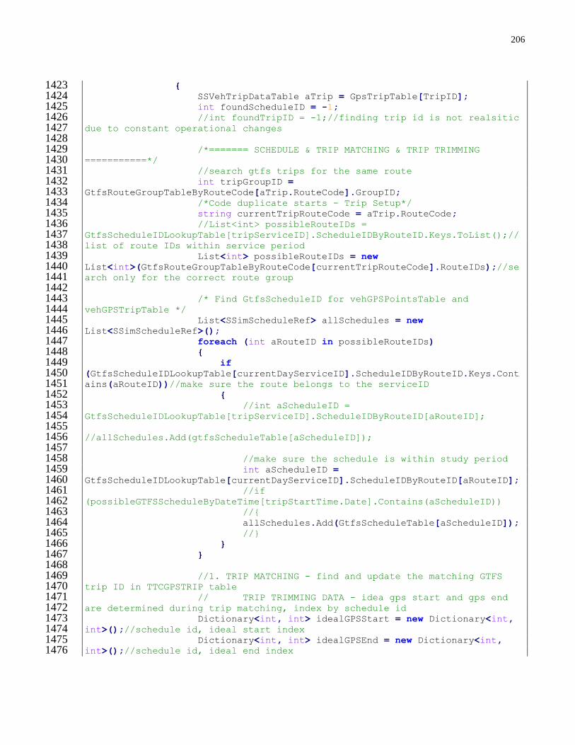
206
{ 1423 SSVehTripDataTable aTrip = GpsTripTable[TripID]; 1424 int foundScheduleID = -1; 1425 //int foundTripID = -1;//finding trip id is not realsitic 1426 due to constant operational changes 1427 1428 /*======= SCHEDULE & TRIP MATCHING & TRIP TRIMMING 1429 ===========*/ 1430 //search gtfs trips for the same route 1431 int tripGroupID = 1432 GtfsRouteGroupTableByRouteCode[aTrip.RouteCode].GroupID; 1433 /*Code duplicate starts - Trip Setup*/ 1434 string currentTripRouteCode = aTrip.RouteCode; 1435 //List<int> possibleRouteIDs = 1436 GtfsScheduleIDLookupTable[tripServiceID].ScheduleIDByRouteID.Keys.ToList();//1437 list of route IDs within service period 1438 List<int> possibleRouteIDs = new 1439 List<int>(GtfsRouteGroupTableByRouteCode[currentTripRouteCode].RouteIDs);//se1440 arch only for the correct route group 1441 1442 /* Find GtfsScheduleID for vehGPSPointsTable and 1443 vehGPSTripTable */ 1444 List<SSimScheduleRef> allSchedules = new 1445 List<SSimScheduleRef>(); 1446 foreach (int aRouteID in possibleRouteIDs) 1447 { 1448 if 1449 (GtfsScheduleIDLookupTable[currentDayServiceID].ScheduleIDByRouteID.Keys.Cont1450 ains(aRouteID))//make sure the route belongs to the serviceID 1451 { 1452 //int aScheduleID = 1453 GtfsScheduleIDLookupTable[tripServiceID].ScheduleIDByRouteID[aRouteID]; 1454 1455 //allSchedules.Add(gtfsScheduleTable[aScheduleID]); 1456 1457 //make sure the schedule is within study period 1458 int aScheduleID = 1459 GtfsScheduleIDLookupTable[currentDayServiceID].ScheduleIDByRouteID[aRouteID]; 1460 //if 1461 (possibleGTFSScheduleByDateTime[tripStartTime.Date].Contains(aScheduleID)) 1462 //{ 1463 allSchedules.Add(GtfsScheduleTable[aScheduleID]); 1464 //} 1465 } 1466 } 1467 1468 //1. TRIP MATCHING - find and update the matching GTFS 1469 trip ID in TTCGPSTRIP table 1470 // TRIP TRIMMING DATA - idea gps start and gps end 1471 are determined during trip matching, index by schedule id 1472 Dictionary<int, int> idealGPSStart = new Dictionary<int, 1473 int>();//schedule id, ideal start index 1474 Dictionary<int, int> idealGPSEnd = new Dictionary<int, 1475 int>();//schedule id, ideal end index 1476
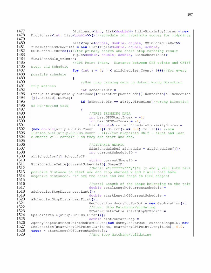
207
Dictionary<int, List<double>> indivProximityScores = new 1477 Dictionary<int, List<double>>();//schedule id, proximity scores for midpoints 1478 1479 List<Tuple<double, double, double, SSimScheduleRef>> 1480 finalMatchedSchedules = new List<Tuple<double, double, double, 1481 SSimScheduleRef>>();//for primary search and start stop matching result 1482 Tuple<double, double, double, SSimScheduleRef> 1483 finalSchedule_trimmed; 1484 //GPS Point Index, Distance between GPS points and GFTFS 1485 stop, and Schedule 1486 for (int j = 0; j < allSchedules.Count; j++)//for every 1487 possible schedule 1488 { 1489 //Use trip triming data to detect wrong Direction 1490 trip matches 1491 int scheduleDir = 1492 GtfsRouteGroupTableByRouteCode[(currentTripRouteCode)].RouteInfo[allSchedules1493 [j].RouteID].DirTag; 1494 if (scheduleDir == aTrip.Direction)//wrong Direction 1495 or non-moving trip 1496 { 1497 //TRIP TRIMMING DATA 1498 int bestGPSStartIndex = -1; 1499 int bestGPSEndIndex = -1; 1500 List<double> currentScheduleProximityScores = 1501 (new double[aTrip.GPSIDs.Count - 1]).Select(x => 0.0).ToList(); //new 1502 List<double>(aTrip.GPSIDs.Count - 1);//for midpoints ONLY - first and last 1503 elements will contain 0 as they are start and end. 1504 1505 //DISTANCE METRIC 1506 SSimScheduleRef aSchedule = allSchedules[j]; 1507 int currentScheduleID = 1508 allSchedules[j].ScheduleID; 1509 string currentShapeID = 1510 GtfsScheduleTable[currentScheduleID].ShapeID; 1511 //Note: w*|*****x***y*|*z (x and y will both have 1512 positive distance to start and end stop whereas w and z will both have 1513 negative distances. "|" are the start and end stops in GTFS shapes) 1514 1515 //Total Length of the Shape belonging to the trip 1516 double totalLengthOfCurrentSchedule = 1517 aSchedule.StopDistances.Last(); 1518 double startLengthOfCurrentSchedule = 1519 aSchedule.StopDistances.First(); 1520 GeoLocation dummyLocForOut = new GeoLocation(); 1521 //Start Stop Matching/Validating 1522 SSVehGPSDataTable startStopGPSPoint = 1523 GpsPointTable[aTrip.GPSIDs.First()]; 1524 double distToStartStop = 1525 AgencyShapeDistFromPointModForGPSPts(out dummyLocForOut, currentShapeID, new 1526 GeoLocation(startStopGPSPoint.Latitude, startStopGPSPoint.Longitude), 0.0, 1527 true) - startLengthOfCurrentSchedule; 1528 //End Stop Matching/Validating 1529

208
SSVehGPSDataTable endStopGPSPoint = 1530 GpsPointTable[aTrip.GPSIDs.Last()]; 1531 double distToEndStop = 1532 totalLengthOfCurrentSchedule - AgencyShapeDistFromPointModForGPSPts(out 1533 dummyLocForOut, currentShapeID, new GeoLocation(endStopGPSPoint.Latitude, 1534 endStopGPSPoint.Longitude), 0.0, true); 1535 //Mid-trip distance offsets - penalize schedule 1536 that doesn't have any overlap or less overlap 1537 double sumMidtripDistDiff = 0;//takes a long time 1538 for (int gpsIDIndex = 1; gpsIDIndex < 1539 (aTrip.GPSIDs.Count - 1); gpsIDIndex++) 1540 { 1541 int gpsID = aTrip.GPSIDs[gpsIDIndex]; 1542 double currentmidTripDist = 1543 ApproxMinDistToShapePath(currentShapeID, new 1544 GeoLocation(GpsPointTable[gpsID].Latitude, GpsPointTable[gpsID].Longitude)); 1545 sumMidtripDistDiff += currentmidTripDist; 1546 1547 currentScheduleProximityScores[gpsIDIndex] = 1548 currentmidTripDist;// Trip Trimming Info 1549 } 1550 //midtripDistDiff = midtripDistDiff / 1551 (aTrip.GPSIDs.Count - 2); 1552 1553 // Trip Trimming Computations 1554 //Note: midpoint distances to start and end stops 1555 are straight line distance evaluations 1556 List<GeoLocation> GPSTripPointLocations = (from r 1557 in aTrip.GPSIDs 1558 select 1559 new GeoLocation(GpsPointTable[r].Latitude, 1560 GpsPointTable[r].Longitude)).ToList(); 1561 GeoLocation startStop = new 1562 GeoLocation(GtfsStopTable[aSchedule.StopIDs.First()].Latitude, 1563 GtfsStopTable[aSchedule.StopIDs.First()].Longitude); 1564 1565 GeoLocation endStop = new 1566 GeoLocation(GtfsStopTable[aSchedule.StopIDs.Last()].Latitude, 1567 GtfsStopTable[aSchedule.StopIDs.Last()].Longitude); 1568 //Write a short method that finds the closest 1569 index, stops once the closest one has been found, rather than keep looking 1570 deeper. Effectively trimming the trips! 1571 bestGPSStartIndex = 1572 GetClosestIndexToStop(GPSTripPointLocations, startStop, true);//closest point 1573 to Start Stop Location (first hit) 1574 bestGPSEndIndex = 1575 GetClosestIndexToStop(GPSTripPointLocations, endStop, false);//closest point 1576 to End Stop Location (first hit) 1577 1578 //Trip Trimming Result/Data 1579 idealGPSStart.Add(aSchedule.ScheduleID, 1580 bestGPSStartIndex); 1581 idealGPSEnd.Add(aSchedule.ScheduleID, 1582 bestGPSEndIndex); 1583

209
indivProximityScores.Add(aSchedule.ScheduleID, 1584 currentScheduleProximityScores);//save calculation for later 1585 1586 //Add ranking score(s) - without trip trimming 1587 //if (distToStartStop >= 0 && distToEndStop >= 0) 1588 //{ 1589 finalMatchedSchedules.Add(new Tuple<double, 1590 double, double, SSimScheduleRef>(Math.Abs(distToStartStop) + 1591 Math.Abs(distToEndStop) + sumMidtripDistDiff, distToStartStop, distToEndStop, 1592 aSchedule));//add as a possible candidate 1593 } 1594 } 1595 //Scoring: ranked schedules and assign the closest 1596 schedule id to the GPS trip 1597 finalMatchedSchedules.Sort((x, y) => 1598 x.Item1.CompareTo(y.Item1));//combined score-ASC 1599 //http://stackoverflow.com/questions/23991802/c-sharp-1600 tuple-list-multiple-sort 1601 foundScheduleID = 1602 finalMatchedSchedules[0].Item4.ScheduleID; 1603 aTrip.GtfsScheduleID = foundScheduleID; 1604 1605 if (foundScheduleID > 0) 1606 { 1607 //2. TRIP TRIMMING OPERATION 1608 //TRIM the trip based on midPointDistToStartStop & 1609 midPointDistToEndStop 1610 //trim end then start 1611 if (((aTrip.GPSIDs.Count - 1 - 1612 idealGPSEnd[foundScheduleID]) > 0) && (idealGPSEnd[foundScheduleID] > 1613 0))//size of removal > 0 1614 { 1615 1616 aTrip.GPSIDs.RemoveRange(idealGPSEnd[foundScheduleID], aTrip.GPSIDs.Count - 1 1617 - idealGPSEnd[foundScheduleID]); 1618 } 1619 if (idealGPSStart[foundScheduleID] > 0)//size of 1620 removal > 0 1621 { 1622 if (idealGPSStart[foundScheduleID] < 1623 idealGPSEnd[foundScheduleID]) 1624 { 1625 aTrip.GPSIDs.RemoveRange(0, 1626 idealGPSStart[foundScheduleID]); 1627 } 1628 else 1629 { 1630 aTrip.GPSIDs = new List<int>();//trip marked 1631 for removal 1632 } 1633 } 1634 //Process trimmed trip - update some fields 1635 if ((aTrip.GPSIDs.Count > 1))//at least 2 points or 1636 trip is flagged and removed & schedule has been found 1637
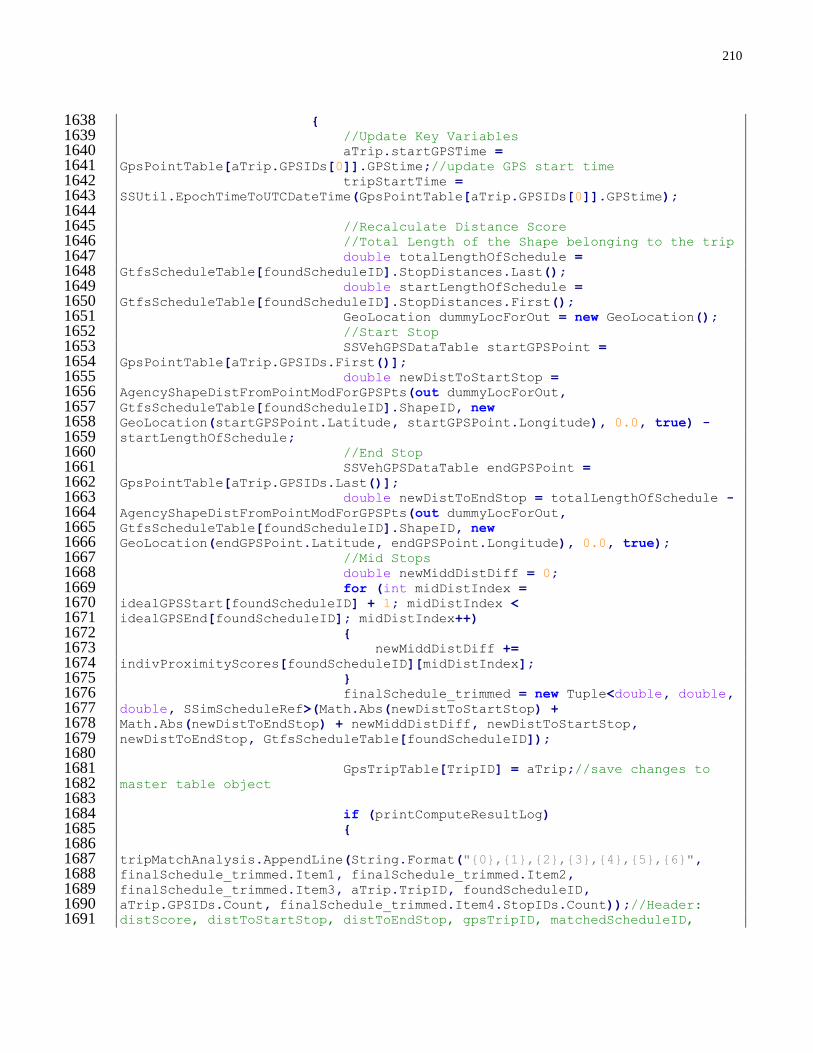
210
{ 1638 //Update Key Variables 1639 aTrip.startGPSTime = 1640 GpsPointTable[aTrip.GPSIDs[0]].GPStime;//update GPS start time 1641 tripStartTime = 1642 SSUtil.EpochTimeToUTCDateTime(GpsPointTable[aTrip.GPSIDs[0]].GPStime); 1643 1644 //Recalculate Distance Score 1645 //Total Length of the Shape belonging to the trip 1646 double totalLengthOfSchedule = 1647 GtfsScheduleTable[foundScheduleID].StopDistances.Last(); 1648 double startLengthOfSchedule = 1649 GtfsScheduleTable[foundScheduleID].StopDistances.First(); 1650 GeoLocation dummyLocForOut = new GeoLocation(); 1651 //Start Stop 1652 SSVehGPSDataTable startGPSPoint = 1653 GpsPointTable[aTrip.GPSIDs.First()]; 1654 double newDistToStartStop = 1655 AgencyShapeDistFromPointModForGPSPts(out dummyLocForOut, 1656 GtfsScheduleTable[foundScheduleID].ShapeID, new 1657 GeoLocation(startGPSPoint.Latitude, startGPSPoint.Longitude), 0.0, true) - 1658 startLengthOfSchedule; 1659 //End Stop 1660 SSVehGPSDataTable endGPSPoint = 1661 GpsPointTable[aTrip.GPSIDs.Last()]; 1662 double newDistToEndStop = totalLengthOfSchedule - 1663 AgencyShapeDistFromPointModForGPSPts(out dummyLocForOut, 1664 GtfsScheduleTable[foundScheduleID].ShapeID, new 1665 GeoLocation(endGPSPoint.Latitude, endGPSPoint.Longitude), 0.0, true); 1666 //Mid Stops 1667 double newMiddDistDiff = 0; 1668 for (int midDistIndex = 1669 idealGPSStart[foundScheduleID] + 1; midDistIndex < 1670 idealGPSEnd[foundScheduleID]; midDistIndex++) 1671 { 1672 newMiddDistDiff += 1673 indivProximityScores[foundScheduleID][midDistIndex]; 1674 } 1675 finalSchedule_trimmed = new Tuple<double, double, 1676 double, SSimScheduleRef>(Math.Abs(newDistToStartStop) + 1677 Math.Abs(newDistToEndStop) + newMiddDistDiff, newDistToStartStop, 1678 newDistToEndStop, GtfsScheduleTable[foundScheduleID]); 1679 1680 GpsTripTable[TripID] = aTrip;//save changes to 1681 master table object 1682 1683 if (printComputeResultLog) 1684 { 1685 1686 tripMatchAnalysis.AppendLine(String.Format("{0},{1},{2},{3},{4},{5},{6}", 1687 finalSchedule_trimmed.Item1, finalSchedule_trimmed.Item2, 1688 finalSchedule_trimmed.Item3, aTrip.TripID, foundScheduleID, 1689 aTrip.GPSIDs.Count, finalSchedule_trimmed.Item4.StopIDs.Count));//Header: 1690 distScore, distToStartStop, distToEndStop, gpsTripID, matchedScheduleID, 1691
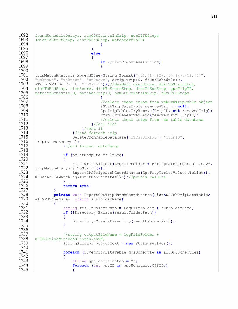
211
foundScheduleDelays, numGPSPointsInTrip, numGTFSStops 1692 (distToStartStop, distToEndStop, matchedTripID) 1693 } 1694 } 1695 else 1696 { 1697 if (printComputeResultLog) 1698 { 1699 1700 tripMatchAnalysis.AppendLine(String.Format("{0},{1},{2},{3},{4},{5},{6}", 1701 "unknown", "unknown", "unknown", aTrip.TripID, foundScheduleID, 1702 aTrip.GPSIDs.Count, "noMatch"));//Header: distScore, distToStartStop, 1703 distToEndStop, timeScore, distToStartStop, distToEndStop, gpsTripID, 1704 matchedScheduleID, matchedTripID, numGPSPointsInTrip, numGTFSStops 1705 } 1706 //delete these trips from vehGPSTripTable object 1707 SSVehTripDataTable removedTrip = null; 1708 GpsTripTable.TryRemove(TripID, out removedTrip); 1709 TripIDToBeRemoved.Add(removedTrip.TripID); 1710 //delete these trips from the table database 1711 }//end else 1712 }//end if 1713 }//end foreach trip 1714 DeleteFromTableDatabase("TTCGPSTRIPS", "TripID", 1715 TripIDToBeRemoved); 1716 }//end foreach dateRange 1717 1718 if (printComputeResultLog) 1719 { 1720 File.WriteAllText(LogFileFolder + @"TripMatchingResult.csv", 1721 tripMatchAnalysis.ToString()); 1722 ExportGPSTripMatchCoordinates(GpsTripTable.Values.ToList(), 1723 @"ScheduleMatchingResultCoordinates\\");//prints results 1724 } 1725 return true; 1726 } 1727 private void ExportGPSTripMatchCoordinates(List<SSVehTripDataTable> 1728 allGPSSchedules, string subFolderName) 1729 { 1730 string resultFolderPath = LogFileFolder + subFolderName; 1731 if (!Directory.Exists(resultFolderPath)) 1732 { 1733 Directory.CreateDirectory(resultFolderPath); 1734 } 1735 1736 //string outputFileName = logFileFolder + 1737 @"GPSTripsWithCoodinates.tsv"; 1738 StringBuilder outputText = new StringBuilder(); 1739 1740 foreach (SSVehTripDataTable gpsSchedule in allGPSSchedules) 1741 { 1742 string gps_coordinates = ""; 1743 foreach (int gpsID in gpsSchedule.GPSIDs) 1744 { 1745
212
gps_coordinates = gps_coordinates + 1746 String.Format("{0},{1}\n", GpsPointTable[gpsID].Latitude, 1747 GpsPointTable[gpsID].Longitude); 1748 } 1749 1750 string gtfs_stop_coordinates = ""; 1751 string gtfs_shape_coordinates = ""; 1752 string shapeID = "-1"; 1753 if (gpsSchedule.GtfsScheduleID > 0)// != -1) 1754 { 1755 SSimScheduleRef gtfsSchedule = 1756 GtfsScheduleTable[gpsSchedule.GtfsScheduleID]; 1757 shapeID = gtfsSchedule.ShapeID; 1758 foreach (int stopID in gtfsSchedule.StopIDs) 1759 { 1760 gtfs_stop_coordinates = gtfs_stop_coordinates + 1761 String.Format("{0},{1}\n", GtfsStopTable[stopID].Latitude, 1762 GtfsStopTable[stopID].Longitude); 1763 } 1764 foreach (Tuple<double, double, double> pathPoint in 1765 GtfsShapeTable[gtfsSchedule.ShapeID].Path) 1766 { 1767 gtfs_shape_coordinates = gtfs_shape_coordinates + 1768 String.Format("{0},{1}\n", pathPoint.Item1, pathPoint.Item2); 1769 } 1770 } 1771 1772 outputText.Append(String.Format("\"GPSTripID: 1773 {0}\"\n{1}\n\"GtfsScheduleID: {2}\"\n{3}\n\"GTFSShapeID: {4}\"\n{5}\n", 1774 gpsSchedule.TripID, gps_coordinates, gpsSchedule.GtfsScheduleID, 1775 gtfs_stop_coordinates, shapeID, gtfs_shape_coordinates)); 1776 File.WriteAllText(resultFolderPath + String.Format("{0}-{1}-1777 ", gpsSchedule.TripID, gpsSchedule.GtfsScheduleID) + 1778 "GPSTripsWithCoodinates.txt", outputText.ToString()); 1779 outputText.Clear(); 1780 } 1781 } 1782
1783

213
A.2.3 Feature Processing Method (DetermineAllFeatureValues)
private bool DetermineAllFeatureValues(bool printComputeResultLog) 1784 { 1785 int numTripAffected = 0; 1786 /*======= I-A1.Initialization of Estimated StopTimes - organize 1787 and process trip information ===========*/ 1788 //find the list of TripIDs that falls within the current date 1789 range 1790 //List<SSVehTripDataTable> allNewTrips = new 1791 List<SSVehTripDataTable>(); 1792 List<int> TripIDToBeRemoved = new List<int>(); 1793 //determine a list of trips needing processing - keep track trip 1794 processing 1795 List<SSVehTripDataTable> allTRIPs_ToBeOrganized = 1796 GpsTripTable.Values.Where(v => v.tripStopIDs == null).ToList(); 1797 numTripAffected += allTRIPs_ToBeOrganized.Count; 1798 List<int> allTripIDs_ToBeOrganized = 1799 allTRIPs_ToBeOrganized.Select(v => v.TripID).ToList(); 1800 allTRIPs_ToBeOrganized.Clear();//clear to min. mem usage 1801 1802 int numTripsRemovedHere = 0; 1803 int numTripsAddedFromSplit = 0; 1804 1805 while (allTripIDs_ToBeOrganized.Count > 0) 1806 { 1807 int TripID = allTripIDs_ToBeOrganized[0]; 1808 List<SSVehTripDataTable> newTripsFromSplit; 1809 bool removeThisTrip = 1810 ProcessAndOrganizeGPSPointsForTrip(TripID, out newTripsFromSplit); 1811 //Note: new trips are added to gpsTripTable() within the 1812 ProcessAndOrganizeGPSPointsForTrip() method. 1813 if (removeThisTrip) 1814 { 1815 TripIDToBeRemoved.Add(TripID);//done processing: deleted 1816 } 1817 if (newTripsFromSplit != null) 1818 { 1819 if (newTripsFromSplit.Count > 0) 1820 { 1821 List<int> newTripIDsFromSplit = (from r in 1822 newTripsFromSplit select r.TripID).ToList(); 1823 numTripsAddedFromSplit += newTripIDsFromSplit.Count; 1824 1825 allTripIDs_ToBeOrganized.AddRange(newTripIDsFromSplit);//additional 1826 processing tasks from split trips 1827 } 1828 } 1829 allTripIDs_ToBeOrganized.Remove(TripID);//done processing: 1830 finished 1831 } 1832 //REMOVE TRIPS 1833 //remove these trips from data object 1834
214
foreach (int removeTripID in TripIDToBeRemoved) 1835 { 1836 //delete these trips from vehGPSTripTable object 1837 SSVehTripDataTable removedTrip = null; 1838 GpsTripTable.TryRemove(removeTripID, out removedTrip); 1839 numTripsRemovedHere++; 1840 } 1841 //delete these trips from the table database 1842 DeleteFromTableDatabase("TTCGPSTRIPS", "TripID", 1843 TripIDToBeRemoved); 1844 TripIDToBeRemoved.Clear(); 1845 1846 /*======= I-A3.Initialization of Estimated StopTimes - compute 1847 then organize by stop id then by trip id ===========*/ 1848 Dictionary<int, Dictionary<int, TimeSpan>> 1849 computedArrivalTimesByStopIDByTripID = new Dictionary<int, Dictionary<int, 1850 TimeSpan>>(); 1851 List<SSVehTripDataTable> allTRIPs_NeedStopTimes = 1852 GpsTripTable.Values.Where(v => v.tripStopArrTimes == null).ToList(); 1853 numTripAffected += allTRIPs_ToBeOrganized.Count; 1854 List<int> allTripIDs_NeedStopTimes = 1855 allTRIPs_NeedStopTimes.Select(v => v.TripID).ToList(); 1856 allTRIPs_NeedStopTimes.Clear(); 1857 foreach (int TripID in GpsTripTable.Keys) 1858 //Parallel.ForEach(allTripIDs_AfterOrganize, (TripID) => 1859 { 1860 Dictionary<int, TimeSpan> TempStopTimesByStopID = new 1861 Dictionary<int, TimeSpan>(); 1862 Dictionary<int, double> TempDwellTimesByStopID; 1863 if (allTripIDs_NeedStopTimes.Contains(TripID))//needs to be 1864 calculated 1865 { 1866 bool complete = 1867 EstimatedArrivalAndDwellAlongScheduleRoute(TripID, out TempStopTimesByStopID, 1868 out TempDwellTimesByStopID);//out List<SSVehGPSDataTable> 1869 if (complete) 1870 { 1871 if 1872 (!computedArrivalTimesByStopIDByTripID.ContainsKey(TripID)) 1873 { 1874 computedArrivalTimesByStopIDByTripID.Add(TripID, 1875 TempStopTimesByStopID); 1876 } 1877 } 1878 else 1879 { 1880 TripIDToBeRemoved.Add(TripID); 1881 //updateGUI_LogBox(String.Format("StopTime 1882 Computation Failed. Line {0}, TripID {1} will be removed", "1732", TripID)); 1883 } 1884 } 1885 else//no need to calculate, can be retrived from saved data 1886 { 1887 //construct TempStopTimesByStopID from saved data 1888
215
for (int tripStopIndex = 0; tripStopIndex < 1889 GpsTripTable[TripID].tripStopIDs.Count; tripStopIndex++) 1890 { 1891 int tripStopID = 1892 GpsTripTable[TripID].tripStopIDs[tripStopIndex]; 1893 TimeSpan tripStopTime = 1894 GpsTripTable[TripID].tripStopArrTimes[tripStopIndex]; 1895 TempStopTimesByStopID.Add(tripStopID, tripStopTime); 1896 } 1897 if 1898 (!computedArrivalTimesByStopIDByTripID.ContainsKey(TripID)) 1899 { 1900 computedArrivalTimesByStopIDByTripID.Add(TripID, 1901 TempStopTimesByStopID); 1902 } 1903 } 1904 }//); 1905 1906 //REMOVE TRIPS 1907 //remove these trips from data object 1908 numTripsRemovedHere = 0; 1909 foreach (int removeTripID in TripIDToBeRemoved) 1910 { 1911 //delete these trips from vehGPSTripTable object 1912 SSVehTripDataTable removedTrip = null; 1913 GpsTripTable.TryRemove(removeTripID, out removedTrip); 1914 numTripsRemovedHere++; 1915 } 1916 //delete these trips from the table database 1917 DeleteFromTableDatabase("TTCGPSTRIPS", "TripID", 1918 TripIDToBeRemoved); 1919 TripIDToBeRemoved.Clear(); 1920 1921 ///*======= I-A4. Initialization of Estimated StopTimes - Update 1922 GPS Trips in the Data Object and Database ===========*/ 1923 ////update all trips variables in the table database 1924 //updateGPSTripInDB(vehGPSTripTable); 1925 1926 /* Start Generic Initializations - 101 */ 1927 //Get a list of possible GPS trips indexed for a particular date 1928 range 1929 //NOTE: GTFS trip found a GPS trip match will be deleted from 1930 list 1931 Dictionary<DateRange, List<int>> GPSTripIDsByDateRange = new 1932 Dictionary<DateRange, List<int>>(); 1933 List<SSVehTripDataTable> allTRIPs_NeedDelayAndHeadway = 1934 GpsTripTable.Values.Where(v => v.tripEstiHeadways == null).ToList(); 1935 numTripAffected += allTRIPs_NeedDelayAndHeadway.Count; 1936 //allTRIPs_NeedDelayAndHeadway.Select(v => v.TripID).ToList(); 1937 List<int> allTripIDs_NeedDelayAndHeadway = (from t in 1938 allTRIPs_NeedDelayAndHeadway.OrderBy(v => v.startGPSTime) select 1939 t.TripID).ToList();//ensure stoptimes processing is in order of time! 1940 allTRIPs_NeedDelayAndHeadway.Clear(); 1941
216
double dateRangeAssignmentToleranceInSecs = 300;//default: 5mins. 1942 Check if dateRanges would overlapp with this 1943 for (int n = 0; n < (AllDateRanges.Count - 1); n++) 1944 { 1945 if ((AllDateRanges[n].end.DateTimeToEpochTime() - 1946 AllDateRanges[n + 1].start.DateTimeToEpochTime()) > 1947 dateRangeAssignmentToleranceInSecs) 1948 { 1949 dateRangeAssignmentToleranceInSecs = 1950 (AllDateRanges[n].end.DateTimeToEpochTime() - AllDateRanges[n + 1951 1].start.DateTimeToEpochTime()); 1952 } 1953 } 1954 foreach (DateRange currentDate in AllDateRanges) 1955 { 1956 GPSTripIDsByDateRange.Add(currentDate, new List<int>()); 1957 List<int> matchedTripIDs = new List<int>();//for debug and 1958 efficiency purpose 1959 1960 //foreach (int TripID in allTripIDs) 1961 for (int i = 0; i < allTripIDs_NeedDelayAndHeadway.Count; 1962 i++) 1963 { 1964 //assign TripID to a dateRange 1965 int TripID = allTripIDs_NeedDelayAndHeadway[i]; 1966 long currentTripStart = 1967 GpsTripTable[TripID].startGPSTime; 1968 if ((currentDate.start.DateTimeToEpochTime() <= 1969 (currentTripStart + dateRangeAssignmentToleranceInSecs)) && 1970 (currentDate.end.DateTimeToEpochTime() >= (currentTripStart - 1971 dateRangeAssignmentToleranceInSecs))) 1972 { 1973 GPSTripIDsByDateRange[currentDate].Add(TripID); 1974 allTripIDs_NeedDelayAndHeadway.RemoveAt(i); 1975 i--; 1976 } 1977 } 1978 } 1979 1980 //MAIN TASK OF THE MEDTHOD 1981 foreach (DateRange currentDay in AllDateRanges) 1982 { 1983 //find current day service id 1984 int currentDayServiceID = 3;//default weekday 1985 DateTime tripStartTime = currentDay.start; 1986 dayType tripDayType = tripStartTime.getDayType(new 1987 dayTypeDefinition()); 1988 foreach (int serviceID in GtfsServicePeriodTable.Keys) 1989 { 1990 if (GtfsServicePeriodTable[serviceID].TypeOfDay == 1991 tripDayType) 1992 { 1993 currentDayServiceID = serviceID; 1994 break; 1995
217
} 1996 } 1997 /* End Generic Initializations - 101 */ 1998 List<int> currentDayTripIDs = 1999 GPSTripIDsByDateRange[currentDay]; 2000 2001 /*======= I-B2.Initialization of Scheduled StopTimes at Stops 2002 ===========*/ 2003 // initialize GTFS stop schedule within this service period, 2004 for all stops (specific to schedule delay calc) 2005 Dictionary<int, List<TimeSpan>> masterGTFSStopInfo = new 2006 Dictionary<int, List<TimeSpan>>();//index stopID, value stopTimes 2007 long bufferTime = 2 * 60;//2*60 mins buffer (from 2008 experimental estimations, 2 hours buffer will cover the worst of cases) 2009 TimeSpan dayStart = 2010 TimeSpan.FromTicks(currentDay.start.AddMinutes(-2011 bufferTime).ToLocalTime().Subtract(currentDay.start.ToLocalTime().Date).Ticks2012 ); 2013 TimeSpan dayEnd = 2014 TimeSpan.FromTicks(currentDay.end.AddMinutes(bufferTime).ToLocalTime().Subtra2015 ct(currentDay.start.ToLocalTime().Date).Ticks); 2016 foreach (SSimStopRef currentStop in GtfsStopTable.Values) 2017 { 2018 List<TimeSpan> singleStopTimes = new List<TimeSpan>(); 2019 2020 //stopTimes for current day service id only 2021 if 2022 (currentStop.scheduledStopTimesByServiceID.ContainsKey(currentDayServiceID)) 2023 { 2024 //SSimStopRef currentStop = 2025 gtfsStopTable[stopID];//check to make sure this is not a pointer 2026 for (int stIndex = 0; stIndex < 2027 currentStop.scheduledStopTimesByServiceID[currentDayServiceID].Count; 2028 stIndex++) 2029 { 2030 TimeSpan aStopTime = 2031 currentStop.scheduledStopTimesByServiceID[currentDayServiceID][stIndex]; 2032 if ((aStopTime.TotalSeconds >= 2033 dayStart.TotalSeconds) && (aStopTime.TotalSeconds <= dayEnd.TotalSeconds)) 2034 { 2035 singleStopTimes.Add(aStopTime); 2036 } 2037 } 2038 masterGTFSStopInfo.Add(currentStop.StopID, 2039 singleStopTimes); 2040 }//end if 2041 //else do nothing 2042 } 2043 2044 /*======= STOP TIMES CALCULATIONS - Done by 2045 computedArrivalTimesByStopIDByTripID() already ===========*/ 2046 2047 /*======= SPEED CALCULATIONS (FOR UTILITY) ===========*/ 2048
218
//TO-DO: technically not need, due to changes to the way data 2049 are processed 2050 for (int tripIndex = 0; tripIndex < currentDayTripIDs.Count; 2051 tripIndex++) 2052 { 2053 //note: assign TimeSpan value in the list to null once 2054 matched to avoid double matching using currentGTFSStopInfo. 2055 int TripID = currentDayTripIDs[tripIndex]; 2056 for (int gpsIndex = 0; gpsIndex < 2057 GpsTripTable[TripID].GPSIDs.Count; gpsIndex++) 2058 { 2059 int gpsID = GpsTripTable[TripID].GPSIDs[gpsIndex]; 2060 double gpsEstiSpeed = -1.0; 2061 if (GpsPointTable[gpsID].EstiAvgSpeed < 0)//check if 2062 it has been calculated already 2063 { 2064 if (gpsIndex > 0 && gpsIndex < 2065 (GpsTripTable[TripID].GPSIDs.Count)) 2066 { 2067 double distToGPS = 2068 GpsPointTable[gpsID].DistFromShapeStart; 2069 long timeToGPS = 2070 GpsPointTable[gpsID].GPStime; 2071 int prevGPSID = 2072 GpsTripTable[TripID].GPSIDs[gpsIndex - 1]; 2073 double distToPrevGPS = 2074 GpsPointTable[prevGPSID].DistFromShapeStart; 2075 long timeToPrevGPS = 2076 GpsPointTable[prevGPSID].GPStime; 2077 gpsEstiSpeed = ((distToGPS - distToPrevGPS) / 2078 (timeToGPS - timeToPrevGPS) * 3.6); 2079 } 2080 else if (gpsIndex == 0) 2081 { 2082 //assume at start of trip, speed is 0 2083 (vehicle generation) 2084 gpsEstiSpeed = 0.0; 2085 } 2086 2087 if (gpsEstiSpeed.Equals(-1.0)) 2088 { 2089 int debug = 0; 2090 } 2091 GpsPointTable[gpsID].EstiAvgSpeed = 2092 Math.Round(gpsEstiSpeed, 1); 2093 } 2094 } 2095 } 2096 /*======= SCHEDULE DELAY CALCULATIONS - A. Matching schedule 2097 stop times with estimated stop times (in 5 smaller steps) ===========*/ 2098 //Previous to this, a list of estimated stopTimes at each 2099 stop of each trip are computed using ProcessAndOrganizeGPSPointsForTrip 2100 (processing) and EstimatedStopTimesAlongScheduleRoute(compute) 2101
219
//Step A-1: simple assignment of observed stop time to 2102 schedule stop time based on lowest time difference 2103 //Step A-2: reverse assignment to reassign observed stop 2104 times with conflicted matches 2105 //Step A-3: Missed Stop Delay Penalization to reassign match 2106 based on missed stop. If stop seq is 1,2,5,6,7, revised is 1,2,3,6,7, where 2107 the delay due to missed stops is penalized. 2108 //Step A-4: backward construction of schedule versus 2109 estimated stopTimes. Based on the fixed match in A-3, construct final actual 2110 and schedule stop time match 2111 //Step A-5. Processing matches for stopTimes final match 2112 results - calculate delay at stops 2113 2114 //A-1: Simple Assignment 2115 Dictionary<int, List<Tuple<int, TimeSpan, int>>> 2116 stopTimesIndexMatchWithTripID_ByStopID = new Dictionary<int, List<Tuple<int, 2117 TimeSpan, int>>>();//Tuple contains stopTimes Index from masterGTFSStopInfo, 2118 estimated/calculated stopTime estimate and TripID - Used also by Headway 2119 Calc! 2120 for (int tripIndex = 0; tripIndex < currentDayTripIDs.Count; 2121 tripIndex++) 2122 { 2123 //note: assign TimeSpan value in the list to null once 2124 matched to avoid double matching using currentGTFSStopInfo. 2125 int TripID = currentDayTripIDs[tripIndex]; 2126 Dictionary<int, Tuple<TimeSpan, TimeSpan>> 2127 Temp_stopTimesMatch_ByStopID = new Dictionary<int, Tuple<TimeSpan, 2128 TimeSpan>>(); 2129 if 2130 (computedArrivalTimesByStopIDByTripID.ContainsKey(TripID)) 2131 { 2132 foreach (int stopID in 2133 GpsTripTable[TripID].tripStopIDs)//note: stops are in order 2134 { 2135 //determine if this trip and stop served multiple 2136 stop times 2137 TimeSpan actualEstiStopTime = 2138 computedArrivalTimesByStopIDByTripID[TripID][stopID]; 2139 //organize computed tuples used for matching 2140 Tuple<int, TimeSpan, int> simpleMatchTuple; 2141 if (masterGTFSStopInfo[stopID].Count > 0) 2142 { 2143 //delay = delay to current stop + missing 2144 stopTimes from previous trips 2145 List<double> delays = (from r in 2146 masterGTFSStopInfo[stopID] select Math.Abs(r.TotalSeconds - 2147 actualEstiStopTime.TotalSeconds)).ToList(); 2148 int stopTimeMatchedIndex = 2149 delays.IndexOf(delays.Min()); 2150 simpleMatchTuple = new Tuple<int, TimeSpan, 2151 int>(stopTimeMatchedIndex, actualEstiStopTime, TripID); 2152 } 2153 else 2154 { 2155
220
simpleMatchTuple = new Tuple<int, TimeSpan, 2156 int>(-1, actualEstiStopTime, TripID);//no schedule - delay will be based on 2157 previous stop if available (later) 2158 } 2159 2160 //add to stopTimesIndexMatchWithTripID_ByStopID 2161 if 2162 (stopTimesIndexMatchWithTripID_ByStopID.ContainsKey(stopID)) 2163 { 2164 2165 stopTimesIndexMatchWithTripID_ByStopID[stopID].Add(simpleMatchTuple); 2166 } 2167 else 2168 { 2169 2170 stopTimesIndexMatchWithTripID_ByStopID.Add(stopID, new List<Tuple<int, 2171 TimeSpan, int>>()); 2172 2173 stopTimesIndexMatchWithTripID_ByStopID[stopID].Add(simpleMatchTuple); 2174 } 2175 }//end foreach 2176 }//end if 2177 }//end for 2178 Dictionary<int, Dictionary<int, Tuple<TimeSpan, TimeSpan>>> 2179 scheduleVsEstimatedStopTimes_ByTripIDByStopID = new Dictionary<int, 2180 Dictionary<int, Tuple<TimeSpan, TimeSpan>>>(); 2181 foreach (int stopID in 2182 stopTimesIndexMatchWithTripID_ByStopID.Keys) 2183 { 2184 //A-2. Reverse Reassignment 2185 // sort stop times matches so duplicated matches are 2186 taken care of: sort by time 2187 stopTimesIndexMatchWithTripID_ByStopID[stopID].Sort((x, 2188 y) => x.Item2.CompareTo(y.Item2)); 2189 // Revise using Backward check for repeated index: check 2190 and see if the list result needs to be revised - no index repeated, if so, 2191 revised according to the TimeSpan values 2192 int prevStopTimesIndex; 2193 int nextStopTimesIndex; 2194 List<int> stopTimesMatchIndexList = (from listItem in 2195 stopTimesIndexMatchWithTripID_ByStopID[stopID] select 2196 listItem.Item1).ToList(); 2197 for (int tupleListIndex = (stopTimesMatchIndexList.Count 2198 - 2); tupleListIndex >= 1; tupleListIndex--)//first and last are not changed, 2199 as they are ref points 2200 { 2201 int TripID = 2202 stopTimesIndexMatchWithTripID_ByStopID[stopID][tupleListIndex].Item3; 2203 prevStopTimesIndex = 2204 stopTimesIndexMatchWithTripID_ByStopID[stopID][tupleListIndex + 1].Item1; 2205 nextStopTimesIndex = 2206 stopTimesIndexMatchWithTripID_ByStopID[stopID][tupleListIndex - 1].Item1; 2207 int currentStopTimesIndex = 2208 stopTimesIndexMatchWithTripID_ByStopID[stopID][tupleListIndex].Item1; 2209

221
//decrease current matched stop index by one only if: 2210 last stop index value is the same as current, next stop index value is not 2211 the same as current, and the (current-1) stop index is not present in the 2212 list, then make current = (current-1) 2213 if (currentStopTimesIndex == prevStopTimesIndex && 2214 currentStopTimesIndex > nextStopTimesIndex && 2215 !stopTimesMatchIndexList.Contains(currentStopTimesIndex - 1)) 2216 { 2217 Tuple<int, TimeSpan, int> revisedTuple = new 2218 Tuple<int, TimeSpan, int>((currentStopTimesIndex - 1), 2219 stopTimesIndexMatchWithTripID_ByStopID[stopID][tupleListIndex].Item2, 2220 stopTimesIndexMatchWithTripID_ByStopID[stopID][tupleListIndex].Item3);//match 2221 with a stop index one previous to 2222 stopTimesMatchIndexList[tupleListIndex] = 2223 (currentStopTimesIndex - 1); 2224 2225 stopTimesIndexMatchWithTripID_ByStopID[stopID][tupleListIndex] = 2226 revisedTuple;//change previous result 2227 } 2228 } 2229 //compute scheduleVsEstimatedStopTimes_ByTripIDByStopID 2230 stopTimesMatchIndexList = (from listItem in 2231 stopTimesIndexMatchWithTripID_ByStopID[stopID] select 2232 listItem.Item1).ToList();//list must be updated 2233 int minIndexBound = stopTimesMatchIndexList.Min();//first 2234 trip's stop is a reference, do not decrease below that. 2235 for (int tupleListIndex = (stopTimesMatchIndexList.Count 2236 - 1); tupleListIndex >= 1; tupleListIndex--) 2237 { 2238 int currentStopTimesIndexMatch = 2239 stopTimesIndexMatchWithTripID_ByStopID[stopID][tupleListIndex].Item1; 2240 int scheduleStopTimesIndex = 2241 currentStopTimesIndexMatch;//may be adjusted 2242 2243 //A-3. Missed Stop Delay Penalization 2244 //trying to find the earliest schedule stopTime that 2245 was not served - final fix of schedule stop time match 2246 while 2247 (!stopTimesMatchIndexList.Contains(scheduleStopTimesIndex - 1) && 2248 (scheduleStopTimesIndex - 1) > minIndexBound) 2249 { 2250 scheduleStopTimesIndex--; 2251 } 2252 if (scheduleStopTimesIndex != 2253 stopTimesIndexMatchWithTripID_ByStopID[stopID][tupleListIndex].Item1)//If 2254 changed by the above while, update tuple data for record. 2255 { 2256 Tuple<int, TimeSpan, int> revisedTuple = new 2257 Tuple<int, TimeSpan, int>((scheduleStopTimesIndex), 2258 stopTimesIndexMatchWithTripID_ByStopID[stopID][tupleListIndex].Item2, 2259 stopTimesIndexMatchWithTripID_ByStopID[stopID][tupleListIndex].Item3);//match 2260 with a stop index one previous to 2261

222
2262 stopTimesIndexMatchWithTripID_ByStopID[stopID][tupleListIndex] = 2263 revisedTuple;//change previous result 2264 } 2265 }//end for tuple matches 2266 for (int tupleListIndex = 0; tupleListIndex < 2267 stopTimesIndexMatchWithTripID_ByStopID[stopID].Count; tupleListIndex++) 2268 { 2269 int gpsTripID = 2270 stopTimesIndexMatchWithTripID_ByStopID[stopID][tupleListIndex].Item3; //final 2271 trip id 2272 TimeSpan estimatedStopTime = 2273 stopTimesIndexMatchWithTripID_ByStopID[stopID][tupleListIndex].Item2; //final 2274 actual stop time 2275 int scheduleStopTimesIndex = 2276 stopTimesIndexMatchWithTripID_ByStopID[stopID][tupleListIndex].Item1; 2277 TimeSpan scheduledStopTime;//final matched schedule 2278 stop time 2279 if (scheduleStopTimesIndex >= 0 && 2280 scheduleStopTimesIndex < masterGTFSStopInfo[stopID].Count) 2281 { 2282 scheduledStopTime = 2283 masterGTFSStopInfo[stopID][scheduleStopTimesIndex]; 2284 } 2285 else 2286 { 2287 scheduledStopTime = new TimeSpan(7, 0, 0, 0, 0); 2288 //7 day as void type 2289 } 2290 //A-4: forward construction of schedule versus 2291 estimated stopTimes. 2292 //= 2293 masterGTFSStopInfo[stopID][scheduleStopTimesIndex]; 2294 //start of: 2295 scheduleVsEstimatedStopTimes_ByTripIDByStopID addition 2296 if 2297 (!scheduleVsEstimatedStopTimes_ByTripIDByStopID.ContainsKey(gpsTripID)) 2298 { 2299 2300 scheduleVsEstimatedStopTimes_ByTripIDByStopID.Add(gpsTripID, new 2301 Dictionary<int, Tuple<TimeSpan, TimeSpan>>()); 2302 } 2303 if 2304 (!scheduleVsEstimatedStopTimes_ByTripIDByStopID[gpsTripID].ContainsKey(stopID2305 )) 2306 { 2307 2308 scheduleVsEstimatedStopTimes_ByTripIDByStopID[gpsTripID].Add(stopID, new 2309 Tuple<TimeSpan, TimeSpan>(scheduledStopTime, estimatedStopTime)); 2310 } 2311 }//end for tuple matches 2312 stopTimesMatchIndexList.Clear();//done using 2313 }//end for stops 2314 2315
223
//A-5: finds the delay at stops 2316 for (int tripIndex = 0; tripIndex < currentDayTripIDs.Count; 2317 tripIndex++) 2318 { 2319 int TripID = currentDayTripIDs[tripIndex]; 2320 //uses scheduleVsEstimatedStopTimes_ByTripIDByStopID to 2321 find estimatedDelay_ByStopID 2322 Dictionary<int, double> estimatedDelay_ByStopID = new 2323 Dictionary<int, double>();//in secs - processed delay 2324 double maxTimeVal = 2 * 24 * 3600; 2325 // double averageDelay = 0.0; 2326 double lastDelay = maxTimeVal; 2327 //foreach (int stopID in 2328 vehGPSTripTable[TripID].tripStopIDs)//note: stops are in order 2329 for (int stopIDIndex = 0; stopIDIndex < 2330 GpsTripTable[TripID].tripStopIDs.Count; stopIDIndex++) 2331 { 2332 int stopID = 2333 GpsTripTable[TripID].tripStopIDs[stopIDIndex]; 2334 double currentDelay = maxTimeVal; 2335 double scheduleTime = 2336 scheduleVsEstimatedStopTimes_ByTripIDByStopID[TripID][stopID].Item1.TotalSeco2337 nds; 2338 double estimatedTime = 2339 scheduleVsEstimatedStopTimes_ByTripIDByStopID[TripID][stopID].Item2.TotalSeco2340 nds; 2341 if (scheduleTime >= maxTimeVal)//should never happen, 2342 if it does, error occurred for this data 2343 { 2344 if (lastDelay < maxTimeVal) 2345 { 2346 currentDelay = lastDelay; 2347 } 2348 else 2349 { 2350 currentDelay = maxTimeVal; 2351 } 2352 } 2353 else 2354 { 2355 currentDelay = estimatedTime - scheduleTime; 2356 } 2357 2358 if (currentDelay < maxTimeVal) 2359 { 2360 //averageDelay = (averageDelay * stopIDIndex + 2361 currentDelay) / (stopIDIndex + 1); 2362 lastDelay = currentDelay; 2363 } 2364 estimatedDelay_ByStopID[stopID] = currentDelay; 2365 }//end for 2366 2367 //process stops with no delay value 2368 double upstreamNearbyDelay = maxTimeVal; 2369
224
for (int stopIDIndex = 0; stopIDIndex < 2370 GpsTripTable[TripID].tripStopIDs.Count; stopIDIndex++) 2371 { 2372 int stopID = 2373 GpsTripTable[TripID].tripStopIDs[stopIDIndex]; 2374 2375 if (stopIDIndex == 0 && 2376 (estimatedDelay_ByStopID[stopID] >= maxTimeVal))//has no upstream, look 2377 downstream 2378 { 2379 int searchStopIDIndex = stopIDIndex; 2380 bool foundVal = false; 2381 while (!foundVal && searchStopIDIndex < 2382 GpsTripTable[TripID].tripStopIDs.Count) 2383 { 2384 int searchStopID = 2385 GpsTripTable[TripID].tripStopIDs[searchStopIDIndex]; 2386 if (estimatedDelay_ByStopID[searchStopID] < 2387 maxTimeVal) 2388 { 2389 estimatedDelay_ByStopID[stopID] = 2390 estimatedDelay_ByStopID[searchStopID]; 2391 foundVal = true; 2392 } 2393 searchStopIDIndex++; 2394 } 2395 2396 if (!foundVal) 2397 { 2398 estimatedDelay_ByStopID[stopID] = -1.0;//bad 2399 trip, no delay can be calculated 2400 } 2401 } 2402 else if (estimatedDelay_ByStopID[stopID] >= 2403 maxTimeVal) 2404 { 2405 estimatedDelay_ByStopID[stopID] = 2406 upstreamNearbyDelay; 2407 } 2408 upstreamNearbyDelay = 2409 estimatedDelay_ByStopID[stopID]; 2410 }//end for stop 2411 2412 //check and validate delays values - stops may be missing 2413 schedule stop times (if exceed studyDurationTolerance) 2414 double studyDurationTolerance = 3600; 2415 //(currentDay.getDurationHours() - (includeOneHourWarmUp ? 1 : 0)) * 2416 3600;//too insensitive 2417 List<double> validDelays = 2418 estimatedDelay_ByStopID.Values.Where(o => o < studyDurationTolerance).Where(o 2419 => o > -studyDurationTolerance).ToList(); 2420 if (validDelays.Count > 0) 2421 { 2422 double avgValidDelays = validDelays.Average(); 2423
225
double lastValidDelay = double.MinValue; 2424 //process stops with missing schedule stop times - 2425 forward pass 2426 for (int stopIDIndex = 0; stopIDIndex < 2427 GpsTripTable[TripID].tripStopIDs.Count; stopIDIndex++) 2428 { 2429 int stopID = 2430 GpsTripTable[TripID].tripStopIDs[stopIDIndex]; 2431 if (Math.Abs(estimatedDelay_ByStopID[stopID] - 2432 avgValidDelays) > studyDurationTolerance) 2433 { 2434 if (lastValidDelay > -100000)// if it has 2435 been assigned 2436 { 2437 estimatedDelay_ByStopID[stopID] = 2438 lastValidDelay; 2439 } 2440 } 2441 else 2442 { 2443 lastValidDelay = 2444 estimatedDelay_ByStopID[stopID]; 2445 } 2446 } 2447 //process stops with missing schedule stop times - 2448 backward pass 2449 for (int stopIDIndex = 2450 (GpsTripTable[TripID].tripStopIDs.Count - 1); stopIDIndex >= 0; stopIDIndex--2451 ) 2452 { 2453 int stopID = 2454 GpsTripTable[TripID].tripStopIDs[stopIDIndex]; 2455 2456 if (Math.Abs(estimatedDelay_ByStopID[stopID] - 2457 avgValidDelays) > studyDurationTolerance) 2458 { 2459 if (lastValidDelay > -100000)// if it has 2460 been assigned 2461 { 2462 estimatedDelay_ByStopID[stopID] = 2463 lastValidDelay; 2464 } 2465 } 2466 else 2467 { 2468 lastValidDelay = 2469 estimatedDelay_ByStopID[stopID]; 2470 } 2471 } 2472 } 2473 2474 //get tripEstiDelays matrix for the trip 2475 List<double> thisTripEstiDelays = new List<double>(); 2476

226
for (int stopIDIndex = 0; stopIDIndex < 2477 GpsTripTable[TripID].tripStopIDs.Count; stopIDIndex++) 2478 { 2479 int stopID = 2480 GpsTripTable[TripID].tripStopIDs[stopIDIndex]; 2481 2482 thisTripEstiDelays.Add(estimatedDelay_ByStopID[stopID]); 2483 }//end for stop 2484 //UPDATE GPS TRIP VARIABLE 2485 GpsTripTable[TripID].tripEstiDelays = new 2486 List<double>(thisTripEstiDelays); 2487 List<double> tempList = 2488 GpsTripTable[TripID].tripEstiDelays.Where(v => v == 2489 maxTimeVal).ToList();//unmatched results 2490 if (tempList.Count > 1) 2491 { 2492 if (!TripIDToBeRemoved.Contains(TripID)) 2493 { 2494 TripIDToBeRemoved.Add(TripID); 2495 } 2496 } 2497 }//end for trip 2498 2499 /*======= OBSERVED HEADWAY CALCULATIONS (AT STOPS) 2500 ===========*/ 2501 //A-1: sort stopTimesIndexMatchWithTripID_ByStopID object 2502 into workable Dictionaries 2503 Dictionary<int, Dictionary<int, double>> 2504 EstiHeadwayByTripIDByStopID = new Dictionary<int, Dictionary<int, double>>(); 2505 foreach (int stopID in 2506 stopTimesIndexMatchWithTripID_ByStopID.Keys) 2507 { 2508 //foreach(Tuple<int,TimeSpan,int> 2509 stopTimesIndexMatchTuple in stopTimesIndexMatchWithTripID_ByStopID[stopID]) 2510 if (stopTimesIndexMatchWithTripID_ByStopID[stopID].Count 2511 > 1) 2512 { 2513 for (int TupleIndex = 0; TupleIndex < 2514 stopTimesIndexMatchWithTripID_ByStopID[stopID].Count; TupleIndex++) 2515 { 2516 //Headway: difference in time between prior 2517 arrival and current arrival at a stop. 2518 //current arrival 2519 Tuple<int, TimeSpan, int> 2520 curStopTimesIndexMatchTuple = 2521 stopTimesIndexMatchWithTripID_ByStopID[stopID][TupleIndex]; 2522 //previous arrival, or next arrival for first 2523 trip at stop 2524 Tuple<int, TimeSpan, int> 2525 nextStopTimesIndexMatchTuple = TupleIndex > 0 ? 2526 stopTimesIndexMatchWithTripID_ByStopID[stopID][TupleIndex - 1] : 2527 stopTimesIndexMatchWithTripID_ByStopID[stopID][TupleIndex + 1];//TupleIndex < 2528 (stopTimesIndexMatchWithTripID_ByStopID[stopID].Count - 1) ? 2529
227
stopTimesIndexMatchWithTripID_ByStopID[stopID][TupleIndex + 1] : 2530 stopTimesIndexMatchWithTripID_ByStopID[stopID][TupleIndex - 1]; 2531 int curTripID = 2532 curStopTimesIndexMatchTuple.Item3; 2533 //A-2: Calculate headway 2534 double estiHeadwayFromStopTimesInSecs = 2535 Math.Abs(curStopTimesIndexMatchTuple.Item2.TotalSeconds - 2536 nextStopTimesIndexMatchTuple.Item2.TotalSeconds); 2537 //A-3: Store calculated headway 2538 if 2539 (!EstiHeadwayByTripIDByStopID.ContainsKey(curTripID)) 2540 { 2541 EstiHeadwayByTripIDByStopID.Add(curTripID, 2542 new Dictionary<int, double>()); 2543 } 2544 if 2545 (!EstiHeadwayByTripIDByStopID[curTripID].ContainsKey(stopID)) 2546 { 2547 2548 EstiHeadwayByTripIDByStopID[curTripID].Add(stopID, 2549 estiHeadwayFromStopTimesInSecs); 2550 } 2551 } 2552 } 2553 //else do not attempt to calculate - rely on 2554 interpolations 2555 }//end foreach stop (trip loop not needed for this comp) 2556 //B-1:Compute and interpolated all observed headway values 2557 for trips' stops, aka process stops with no headway value 2558 for (int tripIndex = 0; tripIndex < currentDayTripIDs.Count; 2559 tripIndex++) 2560 { 2561 int TripID = currentDayTripIDs[tripIndex]; 2562 if (EstiHeadwayByTripIDByStopID.ContainsKey(TripID)) 2563 { 2564 //uses scheduleVsEstimatedStopTimes_ByTripIDByStopID 2565 to find estimatedDelay_ByStopID 2566 //Dictionary<int, double> EstimatedHeadway_ByStopID = 2567 EstiHeadwayByTripIDByStopID[TripID];//in secs - processed delay 2568 for (int stopIDIndex = 0; stopIDIndex < 2569 GpsTripTable[TripID].tripStopIDs.Count; stopIDIndex++) 2570 { 2571 int stopID = 2572 GpsTripTable[TripID].tripStopIDs[stopIDIndex]; 2573 if 2574 (!EstiHeadwayByTripIDByStopID[TripID].ContainsKey(stopID))//attempt to 2575 interpolate 2576 { 2577 int downstreamSearchi = stopIDIndex < 2578 (GpsTripTable[TripID].tripStopIDs.Count - 1) ? stopIDIndex + 1 : stopIDIndex 2579 - 1; 2580 int upstreamSearchj = stopIDIndex > (0) ? 2581 stopIDIndex - 1 : stopIDIndex + 1; 2582 int nearbyStopID_DOWNSTREAM = -1; 2583
228
int nearbyStopID_UPSTREAM = -1; 2584 //try find downstream 2585 while (nearbyStopID_DOWNSTREAM == -1 && 2586 downstreamSearchi <= (GpsTripTable[TripID].tripStopIDs.Count - 1)) 2587 { 2588 if 2589 (EstiHeadwayByTripIDByStopID[TripID].ContainsKey(GpsTripTable[TripID].tripSto2590 pIDs[downstreamSearchi])) 2591 { 2592 nearbyStopID_DOWNSTREAM = 2593 GpsTripTable[TripID].tripStopIDs[downstreamSearchi]; 2594 } 2595 else 2596 { 2597 downstreamSearchi++; 2598 } 2599 } 2600 //try find upstream 2601 while (nearbyStopID_UPSTREAM == -1 && 2602 upstreamSearchj >= 0) 2603 { 2604 if 2605 (EstiHeadwayByTripIDByStopID[TripID].ContainsKey(GpsTripTable[TripID].tripSto2606 pIDs[upstreamSearchj])) 2607 { 2608 nearbyStopID_UPSTREAM = 2609 GpsTripTable[TripID].tripStopIDs[upstreamSearchj]; 2610 } 2611 else 2612 { 2613 upstreamSearchj--; 2614 } 2615 } 2616 //both found, 1 or the other found, or none 2617 found 2618 if (nearbyStopID_DOWNSTREAM >= 0 && 2619 nearbyStopID_UPSTREAM >= 0) 2620 { 2621 double targetStopDist = 2622 GpsTripTable[TripID].tripStopDistances[stopIDIndex]; 2623 double downstreamDist = 2624 GpsTripTable[TripID].tripStopDistances[downstreamSearchi]; 2625 double upstreamDist = 2626 GpsTripTable[TripID].tripStopDistances[upstreamSearchj]; 2627 double downstreamHW = 2628 EstiHeadwayByTripIDByStopID[TripID][nearbyStopID_DOWNSTREAM]; 2629 double upstreamHW = 2630 EstiHeadwayByTripIDByStopID[TripID][nearbyStopID_UPSTREAM]; 2631 2632 double interpolatedHeadway = 2633 ((downstreamHW - upstreamHW) == 0 || (downstreamDist - upstreamDist) == 0 || 2634 (targetStopDist - upstreamDist) < 0) ? (upstreamHW) : (upstreamHW + 2635 (downstreamHW - upstreamHW) / (downstreamDist - upstreamDist) * 2636 (targetStopDist - upstreamDist)); 2637
229
2638 EstiHeadwayByTripIDByStopID[TripID][stopID] = interpolatedHeadway; 2639 } 2640 else if (nearbyStopID_DOWNSTREAM >= 0) 2641 { 2642 2643 EstiHeadwayByTripIDByStopID[TripID][stopID] = 2644 EstiHeadwayByTripIDByStopID[TripID][nearbyStopID_DOWNSTREAM]; 2645 } 2646 else if (nearbyStopID_UPSTREAM >= 0) 2647 { 2648 2649 EstiHeadwayByTripIDByStopID[TripID][stopID] = 2650 EstiHeadwayByTripIDByStopID[TripID][nearbyStopID_UPSTREAM]; 2651 } 2652 //if none of the above conditions can be met, 2653 this stop will be missed => the headway computation for this trip would be 2654 invalid and removed. 2655 }//end if contains key stopid 2656 }//end for stop 2657 //C-1: Assign final headway, post-processed 2658 //get tripEstiHeadways matrix for the trip 2659 List<double> thisTripEstiHeadways = new 2660 List<double>(); 2661 if (GpsTripTable[TripID].tripStopIDs.Count != 2662 EstiHeadwayByTripIDByStopID[TripID].Count) 2663 { 2664 TripIDToBeRemoved.Add(TripID);//remove trips that 2665 can't be processed 2666 } 2667 else 2668 { 2669 for (int stopIDIndex = 0; stopIDIndex < 2670 GpsTripTable[TripID].tripStopIDs.Count; stopIDIndex++) 2671 { 2672 int stopID = 2673 GpsTripTable[TripID].tripStopIDs[stopIDIndex]; 2674 2675 thisTripEstiHeadways.Add(Math.Round(EstiHeadwayByTripIDByStopID[TripID][stopI2676 D], 1)); 2677 }//end for stop 2678 //UPDATE GPS TRIP VARIABLE 2679 GpsTripTable[TripID].tripEstiHeadways = new 2680 List<double>(thisTripEstiHeadways); 2681 //delete criteria 2682 List<double> tempList = new List<double>(); 2683 2684 tempList.AddRange(GpsTripTable[TripID].tripEstiHeadways.Where(v => v >= 2685 currentDay.getDurationSeconds()).ToList());//invalid value 2686 2687 tempList.AddRange(GpsTripTable[TripID].tripEstiDelays.Where(v => v >= 2688 currentDay.getDurationSeconds()).ToList());//invalid value 2689 if (tempList.Count > 1) 2690 { 2691
230
if (!TripIDToBeRemoved.Contains(TripID)) 2692 { 2693 TripIDToBeRemoved.Add(TripID); 2694 } 2695 } 2696 } 2697 }//end if contains key TripID, if this cannot be met => 2698 the headway computation for this trip would be invalid and removed. 2699 }//end for trip 2700 2701 /*======= SCHEDULED HEADWAY CALCULATIONS (AT STOPS) 2702 ===========*/ 2703 //A-1: process all the matching schedule index 2704 Dictionary<int, Dictionary<int, double>> 2705 ScheduleHeadwayByTripIDByStopID = new Dictionary<int, Dictionary<int, 2706 double>>(); 2707 foreach (int stopID in 2708 stopTimesIndexMatchWithTripID_ByStopID.Keys) 2709 { 2710 if (stopTimesIndexMatchWithTripID_ByStopID[stopID].Count 2711 > 1) 2712 { 2713 for (int TupleIndex = 0; TupleIndex < 2714 stopTimesIndexMatchWithTripID_ByStopID[stopID].Count; TupleIndex++) 2715 { 2716 //Schedule Headway: difference in time between 2717 current arrival and prior arrival at a stop, as scheduled. 2718 //current trip 2719 int curTripID = 2720 stopTimesIndexMatchWithTripID_ByStopID[stopID][TupleIndex].Item3; 2721 //current index 2722 int curStopTimeIndex = 2723 stopTimesIndexMatchWithTripID_ByStopID[stopID][TupleIndex].Item1; 2724 ////previous index, or next if this is the first 2725 stop time (less likely) 2726 //int prevStopTimeIndex = curStopTimeIndex > 0 ? 2727 curStopTimeIndex - 1 : curStopTimeIndex + 1; 2728 2729 //only attempt to calculate if matches exist 2730 if (curStopTimeIndex >= 0)// && prevStopTimeIndex 2731 >= 0) 2732 { 2733 // Adjust indices to take the average headway 2734 for 11 arrivals or 10 intervals over that time period. 2735 int maxIndex = 2736 masterGTFSStopInfo[stopID].Count - 1; 2737 int earlierStopTimeIndex = 2738 Math.Max(curStopTimeIndex - 5, 0); 2739 int laterStopTimeIndex = 2740 Math.Min(curStopTimeIndex + 5, maxIndex); 2741 2742 //A-2: Calculate schedule headway 2743 double scheduleHeadwayInSecs = 2744 Math.Abs(masterGTFSStopInfo[stopID][laterStopTimeIndex].TotalSeconds - 2745
231
masterGTFSStopInfo[stopID][earlierStopTimeIndex].TotalSeconds) / 2746 (laterStopTimeIndex - earlierStopTimeIndex); 2747 2748 //A-3: Store calculated headway 2749 if 2750 (!ScheduleHeadwayByTripIDByStopID.ContainsKey(curTripID)) 2751 { 2752 2753 ScheduleHeadwayByTripIDByStopID.Add(curTripID, new Dictionary<int, 2754 double>()); 2755 } 2756 if 2757 (!ScheduleHeadwayByTripIDByStopID[curTripID].ContainsKey(stopID)) 2758 { 2759 2760 ScheduleHeadwayByTripIDByStopID[curTripID].Add(stopID, 2761 scheduleHeadwayInSecs); 2762 } 2763 } 2764 } 2765 } 2766 //else do not attempt to calculate - rely on 2767 interpolations 2768 }//end foreach stop (trip loop not needed for this comp) 2769 //B-1:Compute and interpolated all schedule headway values 2770 for trips' stops, aka process stops with no headway value 2771 for (int tripIndex = 0; tripIndex < currentDayTripIDs.Count; 2772 tripIndex++) 2773 { 2774 int TripID = currentDayTripIDs[tripIndex]; 2775 if (ScheduleHeadwayByTripIDByStopID.ContainsKey(TripID)) 2776 { 2777 for (int stopIDIndex = 0; stopIDIndex < 2778 GpsTripTable[TripID].tripStopIDs.Count; stopIDIndex++) 2779 { 2780 int stopID = 2781 GpsTripTable[TripID].tripStopIDs[stopIDIndex]; 2782 if 2783 (!ScheduleHeadwayByTripIDByStopID[TripID].ContainsKey(stopID))//attempt to 2784 interpolate 2785 { 2786 int downstreamSearchi = stopIDIndex < 2787 (GpsTripTable[TripID].tripStopIDs.Count - 1) ? stopIDIndex + 1 : stopIDIndex 2788 - 1; 2789 int upstreamSearchj = stopIDIndex > (0) ? 2790 stopIDIndex - 1 : stopIDIndex + 1; 2791 int nearbyStopID_DOWNSTREAM = -1; 2792 int nearbyStopID_UPSTREAM = -1; 2793 //try find downstream 2794 while (nearbyStopID_DOWNSTREAM == -1 && 2795 downstreamSearchi <= (GpsTripTable[TripID].tripStopIDs.Count - 1)) 2796 { 2797
232
if 2798 (ScheduleHeadwayByTripIDByStopID[TripID].ContainsKey(GpsTripTable[TripID].tri2799 pStopIDs[downstreamSearchi])) 2800 { 2801 nearbyStopID_DOWNSTREAM = 2802 GpsTripTable[TripID].tripStopIDs[downstreamSearchi]; 2803 } 2804 else 2805 { 2806 downstreamSearchi++; 2807 } 2808 } 2809 //try find upstream 2810 while (nearbyStopID_UPSTREAM == -1 && 2811 upstreamSearchj >= 0) 2812 { 2813 if 2814 (ScheduleHeadwayByTripIDByStopID[TripID].ContainsKey(GpsTripTable[TripID].tri2815 pStopIDs[upstreamSearchj])) 2816 { 2817 nearbyStopID_UPSTREAM = 2818 GpsTripTable[TripID].tripStopIDs[upstreamSearchj]; 2819 } 2820 else 2821 { 2822 upstreamSearchj--; 2823 } 2824 } 2825 //both found, 1 or the other found, or none 2826 found 2827 if (nearbyStopID_DOWNSTREAM >= 0 && 2828 nearbyStopID_UPSTREAM >= 0) 2829 { 2830 double targetStopDist = 2831 GpsTripTable[TripID].tripStopDistances[stopIDIndex]; 2832 double downstreamDist = 2833 GpsTripTable[TripID].tripStopDistances[downstreamSearchi]; 2834 double upstreamDist = 2835 GpsTripTable[TripID].tripStopDistances[upstreamSearchj]; 2836 double downstreamHW = 2837 ScheduleHeadwayByTripIDByStopID[TripID][nearbyStopID_DOWNSTREAM]; 2838 double upstreamHW = 2839 ScheduleHeadwayByTripIDByStopID[TripID][nearbyStopID_UPSTREAM]; 2840 2841 double interpolatedHeadway = 2842 ((downstreamHW - upstreamHW) == 0 || (downstreamDist - upstreamDist) == 0 || 2843 (targetStopDist - upstreamDist) < 0) ? (upstreamHW) : (upstreamHW + 2844 (downstreamHW - upstreamHW) / (downstreamDist - upstreamDist) * 2845 (targetStopDist - upstreamDist)); 2846 2847 ScheduleHeadwayByTripIDByStopID[TripID][stopID] = 2848 Math.Round(interpolatedHeadway, 1); 2849 } 2850 else if (nearbyStopID_DOWNSTREAM >= 0) 2851
233
{ 2852 2853 ScheduleHeadwayByTripIDByStopID[TripID][stopID] = 2854 ScheduleHeadwayByTripIDByStopID[TripID][nearbyStopID_DOWNSTREAM]; 2855 } 2856 else if (nearbyStopID_UPSTREAM >= 0) 2857 { 2858 2859 ScheduleHeadwayByTripIDByStopID[TripID][stopID] = 2860 ScheduleHeadwayByTripIDByStopID[TripID][nearbyStopID_UPSTREAM]; 2861 } 2862 //if none of the above conditions can be met, 2863 this stop will be missed => the headway computation for this trip would be 2864 invalid and removed. 2865 }//end if contains key stopid 2866 }//end for stop 2867 //C-1: Assign final schedule headway, post-processed 2868 //get tripEstiHeadways matrix for the trip 2869 List<double> thisTripScheduledHeadways = new 2870 List<double>(); 2871 if (GpsTripTable[TripID].tripStopIDs.Count != 2872 ScheduleHeadwayByTripIDByStopID[TripID].Count) 2873 { 2874 TripIDToBeRemoved.Add(TripID);//remove trips that 2875 can't be processed 2876 } 2877 else 2878 { 2879 for (int stopIDIndex = 0; stopIDIndex < 2880 GpsTripTable[TripID].tripStopIDs.Count; stopIDIndex++) 2881 { 2882 int stopID = 2883 GpsTripTable[TripID].tripStopIDs[stopIDIndex]; 2884 2885 thisTripScheduledHeadways.Add(Math.Round(ScheduleHeadwayByTripIDByStopID[Trip2886 ID][stopID], 1)); 2887 }//end for stop 2888 //UPDATE GPS TRIP VARIABLE 2889 GpsTripTable[TripID].tripScheduleHeadways = new 2890 List<double>(thisTripScheduledHeadways); 2891 //delete criteria 2892 List<double> tempList = new List<double>(); 2893 2894 tempList.AddRange(GpsTripTable[TripID].tripEstiHeadways.Where(v => v >= 2895 currentDay.getDurationSeconds()).ToList());//invalid value 2896 2897 tempList.AddRange(GpsTripTable[TripID].tripEstiDelays.Where(v => v >= 2898 currentDay.getDurationSeconds()).ToList());//invalid value 2899 if (tempList.Count > 1) 2900 { 2901 if (!TripIDToBeRemoved.Contains(TripID)) 2902 { 2903 TripIDToBeRemoved.Add(TripID); 2904 } 2905
234
} 2906 } 2907 }//end if contains key TripID, if this cannot be met => 2908 the headway computation for this trip would be invalid and removed. 2909 }//end for trip 2910 /*======= tripPrevTripID CALCULATIONS (AT STOPS) 2911 ===========*/ 2912 2913 /*======= Build PreviousTripIDByTripIDByStopID ===========*/ 2914 Dictionary<int, Dictionary<int, int>> 2915 PreviousTripIDByTripIDByStopID = new Dictionary<int, Dictionary<int, int>>(); 2916 foreach (int stopID in 2917 stopTimesIndexMatchWithTripID_ByStopID.Keys) 2918 { 2919 if (stopTimesIndexMatchWithTripID_ByStopID[stopID].Count 2920 > 1) 2921 { 2922 List<int> TripIDListAtStop = (from listItem in 2923 stopTimesIndexMatchWithTripID_ByStopID[stopID] select 2924 listItem.Item3).ToList(); 2925 for (int listIndex = 0; listIndex < 2926 TripIDListAtStop.Count; listIndex++) 2927 { 2928 int curTripID = TripIDListAtStop[listIndex]; 2929 int currentTripStartStopIndex = 2930 GpsTripTable[curTripID].tripStopIDs.IndexOf(stopID); 2931 int curTripNextStop = ((currentTripStartStopIndex 2932 + 1) < GpsTripTable[curTripID].tripStopIDs.Count) ? 2933 (GpsTripTable[curTripID].tripStopIDs[currentTripStartStopIndex + 1]) : (-2934 1);//terminal 2935 int prevTripID = -1; //first trip has no previous 2936 trip id 2937 int matchIndex = listIndex - 1; 2938 if (listIndex > 0) 2939 { 2940 //go over the entire trip list, and assign 2941 only if both stop and end stop match 2942 while (prevTripID == -1 && matchIndex > 0) 2943 { 2944 int potentialPrevTripID = 2945 TripIDListAtStop[matchIndex]; 2946 int prevTripStartStopIndex = 2947 GpsTripTable[potentialPrevTripID].tripStopIDs.IndexOf(stopID); 2948 int nextStopIDForPrevTrip = 2949 ((prevTripStartStopIndex + 1) < 2950 GpsTripTable[potentialPrevTripID].tripStopIDs.Count) ? 2951 (GpsTripTable[potentialPrevTripID].tripStopIDs[prevTripStartStopIndex + 1]) : 2952 (-1);//terminal 2953 if (nextStopIDForPrevTrip == 2954 curTripNextStop) 2955 { 2956 prevTripID = 2957 TripIDListAtStop[matchIndex]; 2958 } 2959
235
matchIndex--; 2960 } 2961 }//else no previous stop 2962 if 2963 (!PreviousTripIDByTripIDByStopID.ContainsKey(curTripID)) 2964 { 2965 PreviousTripIDByTripIDByStopID.Add(curTripID, 2966 new Dictionary<int, int>()); 2967 } 2968 if 2969 (!PreviousTripIDByTripIDByStopID[curTripID].ContainsKey(stopID)) 2970 { 2971 2972 PreviousTripIDByTripIDByStopID[curTripID].Add(stopID, prevTripID); 2973 } 2974 } 2975 } 2976 }//end foreach stop (trip loop not needed for this comp) 2977 //A-2: rearrange, then assign PreviousTripIDByTripIDByStopID 2978 in order of stop to the trip 2979 for (int tripIndex = 0; tripIndex < currentDayTripIDs.Count; 2980 tripIndex++) 2981 { 2982 int TripID = currentDayTripIDs[tripIndex]; 2983 Dictionary<int, int> prevTripID_ByStopID = new 2984 Dictionary<int, int>();//in secs 2985 for (int stopIDIndex = 0; stopIDIndex < 2986 GpsTripTable[TripID].tripStopIDs.Count; stopIDIndex++) 2987 { 2988 int stopID = 2989 GpsTripTable[TripID].tripStopIDs[stopIDIndex]; 2990 int prevTripID = 2991 PreviousTripIDByTripIDByStopID.ContainsKey(TripID) ? 2992 (PreviousTripIDByTripIDByStopID[TripID].ContainsKey(stopID) ? 2993 PreviousTripIDByTripIDByStopID[TripID][stopID] : -1) : -1;//no prev trip id 2994 if didn't exist 2995 prevTripID_ByStopID.Add(stopID, prevTripID); 2996 }//end for 2997 //get tripEstiDelays matrix for the trip 2998 List<int> thisTripPrevTripIDs = new List<int>(); 2999 for (int stopIDIndex = 0; stopIDIndex < 3000 GpsTripTable[TripID].tripStopIDs.Count; stopIDIndex++) 3001 { 3002 int stopID = 3003 GpsTripTable[TripID].tripStopIDs[stopIDIndex]; 3004 thisTripPrevTripIDs.Add(prevTripID_ByStopID[stopID]); 3005 }//end for stop 3006 //UPDATE GPS TRIP VARIABLE 3007 GpsTripTable[TripID].tripPrevTripIDs = new 3008 List<int>(thisTripPrevTripIDs); 3009 }//end for trip 3010 3011 }//end foreach dateRange 3012 3013

236
/*======= I-A2.More Changes to Trip Information (organize and 3014 process trip information) ===========*/ 3015 //add new trips - done with ProcessAndOrganizeGPSPointsForTrip() 3016 & its returns in both data object and database 3017 //remove these trips from data object 3018 //delete these trips from the table database 3019 foreach (int removeTripID in TripIDToBeRemoved) 3020 { 3021 //delete these trips from vehGPSTripTable object 3022 SSVehTripDataTable removedTrip = null; 3023 GpsTripTable.TryRemove(removeTripID, out removedTrip); 3024 } 3025 if (TripIDToBeRemoved.Count > 0) 3026 { 3027 DeleteFromTableDatabase("TTCGPSTRIPS", "TripID", 3028 TripIDToBeRemoved); 3029 } 3030 3031 if (numTripAffected == 0) 3032 { 3033 return false; 3034 } 3035 else 3036 { 3037 return true; 3038 } 3039 } 3040 3041
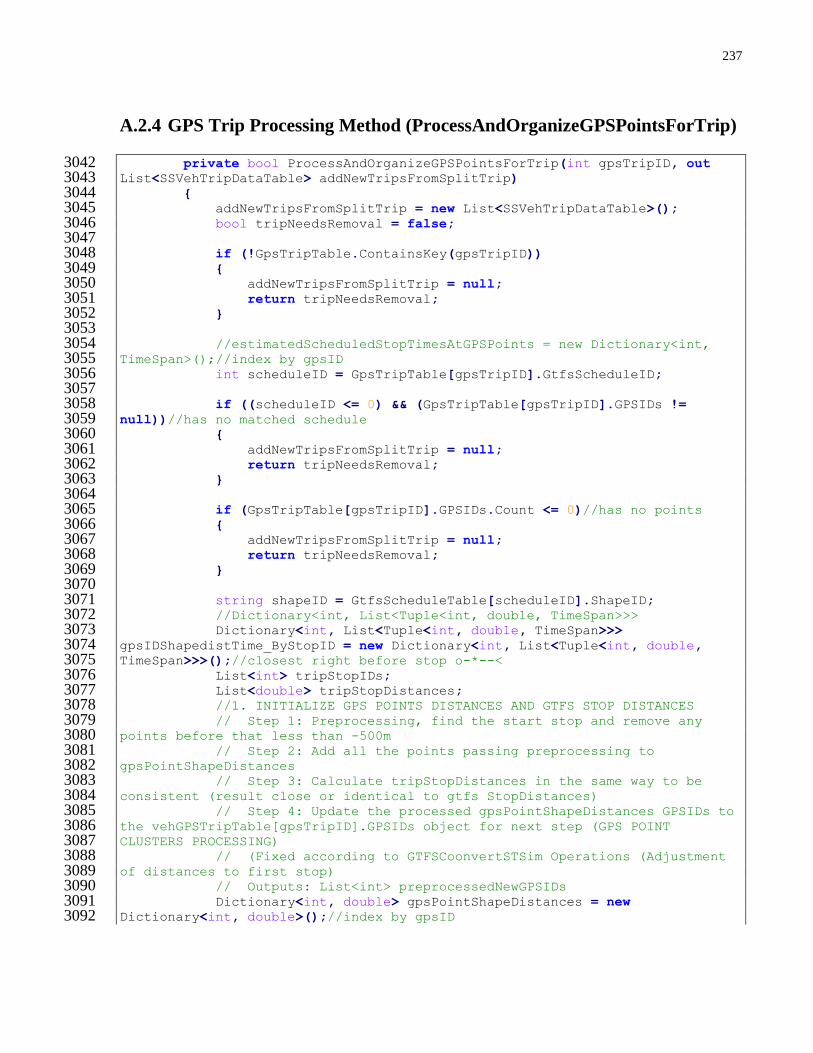
237
A.2.4 GPS Trip Processing Method (ProcessAndOrganizeGPSPointsForTrip)
private bool ProcessAndOrganizeGPSPointsForTrip(int gpsTripID, out 3042 List<SSVehTripDataTable> addNewTripsFromSplitTrip) 3043 { 3044 addNewTripsFromSplitTrip = new List<SSVehTripDataTable>(); 3045 bool tripNeedsRemoval = false; 3046 3047 if (!GpsTripTable.ContainsKey(gpsTripID)) 3048 { 3049 addNewTripsFromSplitTrip = null; 3050 return tripNeedsRemoval; 3051 } 3052 3053 //estimatedScheduledStopTimesAtGPSPoints = new Dictionary<int, 3054 TimeSpan>();//index by gpsID 3055 int scheduleID = GpsTripTable[gpsTripID].GtfsScheduleID; 3056 3057 if ((scheduleID <= 0) && (GpsTripTable[gpsTripID].GPSIDs != 3058 null))//has no matched schedule 3059 { 3060 addNewTripsFromSplitTrip = null; 3061 return tripNeedsRemoval; 3062 } 3063 3064 if (GpsTripTable[gpsTripID].GPSIDs.Count <= 0)//has no points 3065 { 3066 addNewTripsFromSplitTrip = null; 3067 return tripNeedsRemoval; 3068 } 3069 3070 string shapeID = GtfsScheduleTable[scheduleID].ShapeID; 3071 //Dictionary<int, List<Tuple<int, double, TimeSpan>>> 3072 Dictionary<int, List<Tuple<int, double, TimeSpan>>> 3073 gpsIDShapedistTime_ByStopID = new Dictionary<int, List<Tuple<int, double, 3074 TimeSpan>>>();//closest right before stop o-*--< 3075 List<int> tripStopIDs; 3076 List<double> tripStopDistances; 3077 //1. INITIALIZE GPS POINTS DISTANCES AND GTFS STOP DISTANCES 3078 // Step 1: Preprocessing, find the start stop and remove any 3079 points before that less than -500m 3080 // Step 2: Add all the points passing preprocessing to 3081 gpsPointShapeDistances 3082 // Step 3: Calculate tripStopDistances in the same way to be 3083 consistent (result close or identical to gtfs StopDistances) 3084 // Step 4: Update the processed gpsPointShapeDistances GPSIDs to 3085 the vehGPSTripTable[gpsTripID].GPSIDs object for next step (GPS POINT 3086 CLUSTERS PROCESSING) 3087 // (Fixed according to GTFSCoonvertSTSim Operations (Adjustment 3088 of distances to first stop) 3089 // Outputs: List<int> preprocessedNewGPSIDs 3090 Dictionary<int, double> gpsPointShapeDistances = new 3091 Dictionary<int, double>();//index by gpsID 3092
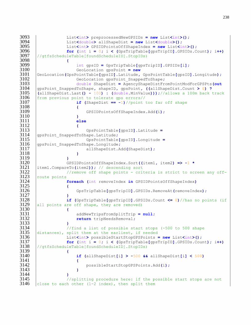
238
List<int> preprocessedNewGPSIDs = new List<int>(); 3093 List<double> allShapeDist = new List<double>(); 3094 List<int> GPSIDPointsOffShapeIndex = new List<int>(); 3095 for (int i = 0; i < (GpsTripTable[gpsTripID].GPSIDs.Count); i++) 3096 //gtfsScheduleTable[foundScheduleID].StopIDs) 3097 { 3098 int gpsID = GpsTripTable[gpsTripID].GPSIDs[i]; 3099 GeoLocation gpsPoint = new 3100 GeoLocation(GpsPointTable[gpsID].Latitude, GpsPointTable[gpsID].Longitude); 3101 GeoLocation gpsPoint_SnappedToShape; 3102 double ShapeDist = AgencyShapeDistFromPointModForGPSPts(out 3103 gpsPoint_SnappedToShape, shapeID, gpsPoint, ((allShapeDist.Count > 0) ? 3104 (allShapeDist.Last() - 100) : (double.MinValue)));//allows a 100m back track 3105 from previous point to tolerate gps errors// 3106 if (ShapeDist == -1)//point too far off shape 3107 { 3108 GPSIDPointsOffShapeIndex.Add(i); 3109 } 3110 else 3111 { 3112 GpsPointTable[gpsID].Latitude = 3113 gpsPoint_SnappedToShape.Latitude; 3114 GpsPointTable[gpsID].Longitude = 3115 gpsPoint_SnappedToShape.Longitude; 3116 allShapeDist.Add(ShapeDist); 3117 } 3118 } 3119 GPSIDPointsOffShapeIndex.Sort((item1, item2) => -1 * 3120 item1.CompareTo(item2)); // descending sort 3121 //remove off shape points - criteria is strict to screen any off-3122 route points 3123 foreach (int removeIndex in GPSIDPointsOffShapeIndex) 3124 { 3125 GpsTripTable[gpsTripID].GPSIDs.RemoveAt(removeIndex); 3126 } 3127 if (GpsTripTable[gpsTripID].GPSIDs.Count <= 0)//has no points (if 3128 all points are off shape, they are removed) 3129 { 3130 addNewTripsFromSplitTrip = null; 3131 return tripNeedsRemoval; 3132 } 3133 //find a list of possible start stops (-500 to 500 shape 3134 distances), split them at the earliest, if needed 3135 List<int> possibleStartStopGPSPoints = new List<int>(); 3136 for (int i = 0; i < (GpsTripTable[gpsTripID].GPSIDs.Count); i++) 3137 //gtfsScheduleTable[foundScheduleID].StopIDs) 3138 { 3139 if (allShapeDist[i] > -500 && allShapeDist[i] < 500) 3140 { 3141 possibleStartStopGPSPoints.Add(i); 3142 } 3143 } 3144 //splitting procedure here: if the possible start stops are not 3145 close to each other (1-2 index), then split them 3146
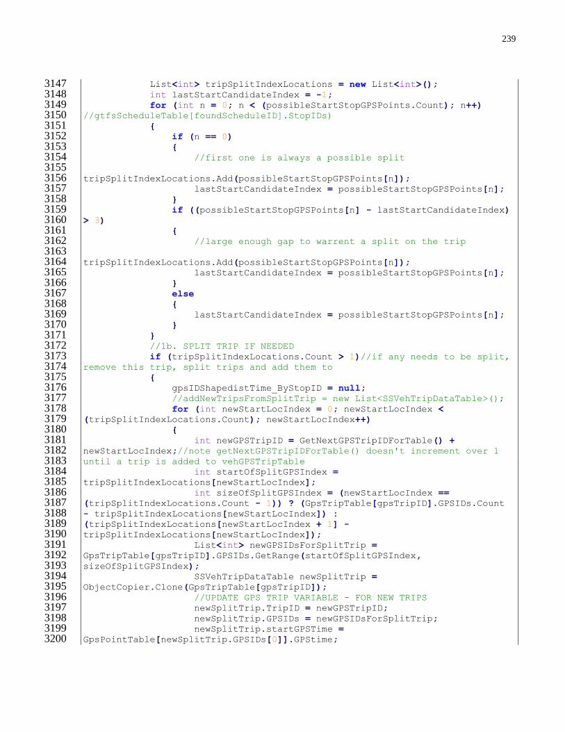
239
List<int> tripSplitIndexLocations = new List<int>(); 3147 int lastStartCandidateIndex = -1; 3148 for (int n = 0; n < (possibleStartStopGPSPoints.Count); n++) 3149 //gtfsScheduleTable[foundScheduleID].StopIDs) 3150 { 3151 if (n == 0) 3152 { 3153 //first one is always a possible split 3154 3155 tripSplitIndexLocations.Add(possibleStartStopGPSPoints[n]); 3156 lastStartCandidateIndex = possibleStartStopGPSPoints[n]; 3157 } 3158 if ((possibleStartStopGPSPoints[n] - lastStartCandidateIndex) 3159 > 3) 3160 { 3161 //large enough gap to warrent a split on the trip 3162 3163 tripSplitIndexLocations.Add(possibleStartStopGPSPoints[n]); 3164 lastStartCandidateIndex = possibleStartStopGPSPoints[n]; 3165 } 3166 else 3167 { 3168 lastStartCandidateIndex = possibleStartStopGPSPoints[n]; 3169 } 3170 } 3171 //1b. SPLIT TRIP IF NEEDED 3172 if (tripSplitIndexLocations.Count > 1)//if any needs to be split, 3173 remove this trip, split trips and add them to 3174 { 3175 gpsIDShapedistTime_ByStopID = null; 3176 //addNewTripsFromSplitTrip = new List<SSVehTripDataTable>(); 3177 for (int newStartLocIndex = 0; newStartLocIndex < 3178 (tripSplitIndexLocations.Count); newStartLocIndex++) 3179 { 3180 int newGPSTripID = GetNextGPSTripIDForTable() + 3181 newStartLocIndex;//note getNextGPSTripIDForTable() doesn't increment over 1 3182 until a trip is added to vehGPSTripTable 3183 int startOfSplitGPSIndex = 3184 tripSplitIndexLocations[newStartLocIndex]; 3185 int sizeOfSplitGPSIndex = (newStartLocIndex == 3186 (tripSplitIndexLocations.Count - 1)) ? (GpsTripTable[gpsTripID].GPSIDs.Count 3187 - tripSplitIndexLocations[newStartLocIndex]) : 3188 (tripSplitIndexLocations[newStartLocIndex + 1] - 3189 tripSplitIndexLocations[newStartLocIndex]); 3190 List<int> newGPSIDsForSplitTrip = 3191 GpsTripTable[gpsTripID].GPSIDs.GetRange(startOfSplitGPSIndex, 3192 sizeOfSplitGPSIndex); 3193 SSVehTripDataTable newSplitTrip = 3194 ObjectCopier.Clone(GpsTripTable[gpsTripID]); 3195 //UPDATE GPS TRIP VARIABLE - FOR NEW TRIPS 3196 newSplitTrip.TripID = newGPSTripID; 3197 newSplitTrip.GPSIDs = newGPSIDsForSplitTrip; 3198 newSplitTrip.startGPSTime = 3199 GpsPointTable[newSplitTrip.GPSIDs[0]].GPStime; 3200
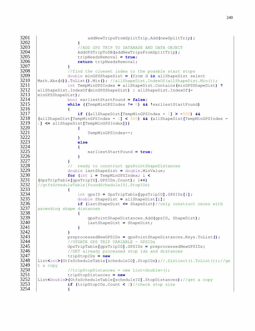
240
addNewTripsFromSplitTrip.Add(newSplitTrip); 3201 } 3202 //ADD GPS TRIP TO DATABASE AND DATA OBJECT 3203 AddGPSTripToDB(addNewTripsFromSplitTrip); 3204 tripNeedsRemoval = true; 3205 return tripNeedsRemoval; 3206 } 3207 //find the cloeset index to the possble start stops 3208 double minGPSShapeDist = (from d in allShapeDist select 3209 Math.Abs(d)).ToList().Min(); //allShapeDist.IndexOf(allShapeDist.Min()); 3210 int TempMinGPSIndex = allShapeDist.Contains(minGPSShapeDist) ? 3211 allShapeDist.IndexOf(minGPSShapeDist) : allShapeDist.IndexOf(-3212 minGPSShapeDist); 3213 bool earliestStartFound = false; 3214 while ((TempMinGPSIndex != 0) && !earliestStartFound) 3215 { 3216 if ((allShapeDist[TempMinGPSIndex - 1] > -500) && 3217 (allShapeDist[TempMinGPSIndex - 1] < 500) && (allShapeDist[TempMinGPSIndex - 3218 1] <= allShapeDist[TempMinGPSIndex])) 3219 { 3220 TempMinGPSIndex--; 3221 } 3222 else 3223 { 3224 earliestStartFound = true; 3225 } 3226 } 3227 // ready to construct gpsPointShapeDistances 3228 double lastShapeDist = double.MinValue; 3229 for (int i = TempMinGPSIndex; i < 3230 (GpsTripTable[gpsTripID].GPSIDs.Count); i++) 3231 //gtfsScheduleTable[foundScheduleID].StopIDs) 3232 { 3233 int gpsID = GpsTripTable[gpsTripID].GPSIDs[i]; 3234 double ShapeDist = allShapeDist[i]; 3235 if (lastShapeDist <= ShapeDist)//only construct onces with 3236 ascending shape distances 3237 { 3238 gpsPointShapeDistances.Add(gpsID, ShapeDist); 3239 lastShapeDist = ShapeDist; 3240 } 3241 } 3242 preprocessedNewGPSIDs = gpsPointShapeDistances.Keys.ToList(); 3243 //UPDATE GPS TRIP VARIABLE - GPSIDs 3244 GpsTripTable[gpsTripID].GPSIDs = preprocessedNewGPSIDs; 3245 //GET already processed stop ids and distances 3246 tripStopIDs = new 3247 List<int>(GtfsScheduleTable[scheduleID].StopIDs);//.Distinct().ToList());//ge3248 t a copy 3249 //tripStopDistances = new List<double>(); 3250 tripStopDistances = new 3251 List<double>(GtfsScheduleTable[scheduleID].StopDistances);//get a copy 3252 if (tripStopIDs.Count < 2)//check stop size 3253 { 3254

241
tripNeedsRemoval = true; 3255 gpsIDShapedistTime_ByStopID = null; 3256 return tripNeedsRemoval; 3257 } 3258 ////Old procedure, less computationally efficient 3259 //if (numHeaders > 8) 3260 // newStopTimes.DistanceToStop = splitLine[8] != "" ? 3261 Double.Parse(splitLine[8]) * 1000 : 0; //*1000 for km to m 3262 conversion 3263 //else 3264 // newStopTimes.DistanceToStop = -1; 3265 //StopTimes.Add(newStopTimes); 3266 //// Trip stop distances compute 1: distances from shape start 3267 //for (int i = 0; i < (tripStopIDs.Count); i++) 3268 //{ 3269 // int stopID = tripStopIDs[i]; 3270 // GeoLocation stopPoint = new 3271 GeoLocation(gtfsStopTable[stopID].Latitude, gtfsStopTable[stopID].Longitude); 3272 3273 // bool notfirstOcc; 3274 // if (tripStopDistances.Count > 1)// && 3275 ListTrips[stopInfo.TripID].StopInfo[1].Stop == newSInfo.Stop) 3276 // { 3277 // notfirstOcc = true; 3278 // } 3279 // else 3280 // { 3281 // notfirstOcc = false; 3282 // } 3283 // tripStopDistances.Add(AgencyShapeDistFromPoint(shapeID, 3284 stopPoint, notfirstOcc ? tripStopDistances[i - 1] : 0)); 3285 // //newSInfo.DistFromFirstStop = stopInfo.DistanceToStop != -3286 1 ? stopInfo.DistanceToStop : 3287 AgencyShapeDistFromPoint(ListTrips[stopInfo.TripID].Shape.ShapeID, 3288 stopInfo.StopID, agencyID, notfirstOcc ? 3289 ListTrips[stopInfo.TripID].StopInfo[stopInfo.StopSequence - 3290 1].DistFromFirstStop : 0); 3291 // //if (tripStopDistances.Count == 1 && 3292 ListTrips[stopInfo.TripID].StopInfo[1].DistFromFirstStop > 3293 newSInfo.DistFromFirstStop) 3294 // //{ 3295 // // 3296 ListTrips[stopInfo.TripID].StopInfo[1].DistFromFirstStop = 0; 3297 // //} 3298 //} 3299 int firstStopID = tripStopIDs[0]; 3300 GeoLocation FirstStopPt = new 3301 GeoLocation(GtfsStopTable[firstStopID].Latitude, 3302 GtfsStopTable[firstStopID].Longitude); 3303 int secondStopID = tripStopIDs[1]; 3304 GeoLocation secondStopPt = new 3305 GeoLocation(GtfsStopTable[secondStopID].Latitude, 3306 GtfsStopTable[secondStopID].Longitude); 3307 // Trip stop distances compute 2: Shape Distance adjustments 3308

242
double firstStopDist = ShapeDistFromPoint(shapeID, FirstStopPt, 3309 tripStopDistances[1]); 3310 bool secondStopFromShapeStart = SecondStopFromShapeStart(shapeID, 3311 FirstStopPt, firstStopDist, secondStopPt, tripStopDistances[1]); 3312 //tripStopDistances[0] = firstStopDist; 3313 if (secondStopFromShapeStart == false) 3314 { 3315 for (int i = 0; i < (GpsTripTable[gpsTripID].GPSIDs.Count); 3316 i++) 3317 { 3318 int gpsID = GpsTripTable[gpsTripID].GPSIDs[i]; 3319 gpsPointShapeDistances[gpsID] += firstStopDist; 3320 } 3321 //// trip stop distances compute 3322 //for (int i = 1; i < (tripStopIDs.Count); i++) 3323 //{ 3324 // tripStopDistances[i] += firstStopDist; 3325 //} 3326 } 3327 //2. GPS POINT CLUSTERS PROCESSING 3328 // Groups gps clusters together to ensure points aren't redundant 3329 and/or back tracking 3330 // Step 1: go through gps points order by GPStime. If the 3331 current gps point is very close to the previous (~10m, add to a cluster). 3332 // If they are not close, check if the gps point has 3333 positive velocity relative to last gps point. 3334 // If yes, start a new cluster, if no, remove the gps 3335 point from the trip and update gps trip id 3336 // Step 2: after all the gps points are processed into their own 3337 clusters, for cluster with more than 2 points, find the earliest point and 3338 latest point 3339 // Then, remove all other gps points from trip and 3340 update gps trip id 3341 // The chosen two points will take coordinates of the 3342 cluster centroid, with their original GPStimes. 3343 // Step 3: now that the cluster processing has been conducted 3344 for all gps points in the trip, it is now ready to be used for purpose of 3345 variable calculations. 3346 // Outputs: List<int> clusterProcessedNewGPSIDs 3347 //Preprocessing, find the start stop and trim the trip 3348 List<List<int>> gpsClusters = new List<List<int>>(); 3349 List<int> clusterProcessedNewGPSIDs = new List<int>(); 3350 List<int> currentGPSCluster = new List<int>(); 3351 currentGPSCluster.Add(GpsTripTable[gpsTripID].GPSIDs[0]); 3352 bool isClusterNew = true; 3353 int startOfClusterGPSID = GpsTripTable[gpsTripID].GPSIDs[0]; 3354 //group points into many clusters 3355 for (int i = 1; i < (GpsTripTable[gpsTripID].GPSIDs.Count); i++) 3356 //gtfsScheduleTable[foundScheduleID].StopIDs) 3357 { 3358 startOfClusterGPSID = isClusterNew ? 3359 GpsTripTable[gpsTripID].GPSIDs[i - 1] : startOfClusterGPSID; 3360 int currentGPSID = GpsTripTable[gpsTripID].GPSIDs[i]; 3361

243
double displacement = gpsPointShapeDistances[currentGPSID] - 3362 gpsPointShapeDistances[startOfClusterGPSID]; 3363 //double deltaTime = (vehGPSPointsTable[currentGPSID].GPStime 3364 - vehGPSPointsTable[prevGPSID].GPStime); 3365 3366 if (Math.Abs(displacement) < ClusterDisplacementTolerance) 3367 //close by points 3368 { 3369 //add to current cluster 3370 currentGPSCluster.Add(currentGPSID); 3371 isClusterNew = false; 3372 } 3373 else //large enough displacement results in a new cluster 3374 { 3375 //finish adding current cluster to master gpsClusters and 3376 int[] TempCluster = new int[currentGPSCluster.Count]; 3377 currentGPSCluster.CopyTo(TempCluster); 3378 gpsClusters.Add(TempCluster.ToList()); 3379 //start a new cluster 3380 isClusterNew = true; 3381 currentGPSCluster = null; 3382 currentGPSCluster = new List<int>(); 3383 currentGPSCluster.Add(currentGPSID); 3384 } 3385 //add final point/cluster 3386 if (i == (GpsTripTable[gpsTripID].GPSIDs.Count - 1)) 3387 { 3388 //finish adding current cluster to master gpsClusters and 3389 int[] TempCluster = new int[currentGPSCluster.Count]; 3390 currentGPSCluster.CopyTo(TempCluster); 3391 gpsClusters.Add(TempCluster.ToList()); 3392 } 3393 } 3394 //processing to remove non-revenue or back-tracking clusters 3395 for (int i_group = 0; i_group < (gpsClusters.Count - 1); 3396 i_group++) 3397 { 3398 //due to nature of comparsions, last gpsCluster will be 3399 automatically retained 3400 List<int> thisGPSCluster = gpsClusters[i_group]; 3401 List<int> nextGPSCluster = gpsClusters[i_group + 1]; 3402 int thisGPSID = thisGPSCluster[0];//look at first pt of 3403 cluster 3404 int nextGPSID = nextGPSCluster[0];//look at first pt of 3405 cluster 3406 double displacement = gpsPointShapeDistances[nextGPSID] - 3407 gpsPointShapeDistances[thisGPSID]; 3408 double deltaTime = (GpsPointTable[nextGPSID].GPStime - 3409 GpsPointTable[thisGPSID].GPStime); 3410 //check if the cluster is decreasing in shape distance, if so 3411 if ((displacement) / (deltaTime) < 0.0) //needs a positive 3412 velocity or else the cluster is removed 3413 { 3414 //likely due to displacment 3415

244
gpsClusters.RemoveAt(i_group); 3416 i_group--; 3417 } 3418 } 3419 //process all gps clusters into a list of new GPS IDs --> can 3420 potentially compute dwell time from this! 3421 foreach (List<int> aGPSCluster in gpsClusters) 3422 { 3423 if (aGPSCluster.Count <= 2) 3424 { 3425 clusterProcessedNewGPSIDs.AddRange(aGPSCluster); 3426 } 3427 else 3428 { 3429 clusterProcessedNewGPSIDs.Add(aGPSCluster[0]); 3430 3431 clusterProcessedNewGPSIDs.Add(aGPSCluster[aGPSCluster.Count - 1]); 3432 }//end else 3433 }//end foreach 3434 //final checks of distances and times - ignores first points 3435 though (cannot compare) - similar check done before on clusters checking 3436 first point 3437 //foreach (int gpsID in newGPSIDs) 3438 List<int> GPSIDsToBeRemovedGPSErrors = new List<int>(); 3439 for (int centerPtIndex = 1; centerPtIndex < 3440 (clusterProcessedNewGPSIDs.Count); centerPtIndex++) 3441 { 3442 long timeLeft = 3443 GpsPointTable[clusterProcessedNewGPSIDs[centerPtIndex - 1]].GPStime; 3444 long timeCtr = 3445 GpsPointTable[clusterProcessedNewGPSIDs[centerPtIndex]].GPStime; 3446 //long timeRight = vehGPSPointsTable[newGPSIDs[centerPtIndex 3447 + 1]].GPStime; 3448 double shapeDistLeft = 3449 gpsPointShapeDistances[clusterProcessedNewGPSIDs[centerPtIndex - 1]]; 3450 double shapeDistCtr = 3451 gpsPointShapeDistances[clusterProcessedNewGPSIDs[centerPtIndex]]; 3452 //double shapeDistRight = 3453 gpsPointShapeDistances[newGPSIDs[centerPtIndex + 1]]; 3454 //double velocity1 = (shapeDistCtr - shapeDistLeft) / 3455 (timeCtr - timeLeft) * 3.6; 3456 //double velocity2 = (shapeDistRight - shapeDistCtr) / 3457 (timeRight - timeCtr) * 3.6; 3458 if ((shapeDistCtr - shapeDistLeft) < 0 && 3459 Math.Abs(shapeDistCtr - shapeDistLeft) < 10) 3460 { 3461 //very small negative distance difference, the vehicle is 3462 probably stopped, change its shape dist to ctr 3463 3464 gpsPointShapeDistances[clusterProcessedNewGPSIDs[centerPtIndex - 1]] = 3465 gpsPointShapeDistances[clusterProcessedNewGPSIDs[centerPtIndex]]; 3466 } 3467 if ((shapeDistCtr - shapeDistLeft) < 0 || (timeCtr - 3468 timeLeft) < 0)//case: raced ahead 3469

245
{ 3470 3471 GPSIDsToBeRemovedGPSErrors.Add(clusterProcessedNewGPSIDs[centerPtIndex]); 3472 } 3473 else if ((timeCtr - timeLeft) > (5 * 60))//gps point gap too 3474 larger (>5mins), rest of trip's gps points are may not be valid 3475 { 3476 3477 GPSIDsToBeRemovedGPSErrors.AddRange(clusterProcessedNewGPSIDs.GetRange(center3478 PtIndex, clusterProcessedNewGPSIDs.Count - centerPtIndex)); 3479 break; 3480 } 3481 } 3482 foreach (int removeGPS in GPSIDsToBeRemovedGPSErrors) 3483 { 3484 clusterProcessedNewGPSIDs.Remove(removeGPS); 3485 } 3486 //UPDATE GPS TRIP VARIABLE - GPSIDs 3487 GpsTripTable[gpsTripID].GPSIDs = clusterProcessedNewGPSIDs; 3488 //3. COMPUTE gpsID_DistFromStartMatchByStopID 3489 // Organize the gps points in relative positions to the gtfs 3490 stops, ordered by their distance from the stop downstream 3491 // * points can only be added to stop IN ORDER. This prevents 3492 back tracked points or travels in reversed Direction. 3493 // Outputs: List<int> stopOrderProcessedNewGPSIDs 3494 int currentStopIndexProcessing = -1;//may not add to a stop if it 3495 is "completed"/next one has started 3496 List<int> stopOrderProcessedNewGPSIDs = new List<int>(); 3497 for (int i = 0; i < (GpsTripTable[gpsTripID].GPSIDs.Count); i++) 3498 //(vehGPSTripTable[gpsTripID].GPSIDs.Count); i++) 3499 //gtfsScheduleTable[foundScheduleID].StopIDs) 3500 { 3501 int gpsID = GpsTripTable[gpsTripID].GPSIDs[i]; 3502 double distOfGPSFromStart = gpsPointShapeDistances[gpsID]; 3503 GeoLocation gpsPoint = new 3504 GeoLocation(GpsPointTable[gpsID].Latitude, GpsPointTable[gpsID].Longitude); 3505 TimeSpan gpsTimeSpan = 3506 SSUtil.EpochTimeToLocalDateTime(GpsPointTable[gpsID].GPStime).DateTimeToTimeS3507 panFromLastLocalMidnight(); 3508 //note: if the gps point is less than 50m past the stop, it 3509 is added. This allows better dwell time determinations for 20s data 3510 List<double> allResult = new List<double>();// = (from r in 3511 tripStopDistances select ((r - distOfGPSFromStart) >= -50 ? (r - 3512 distOfGPSFromStart) : double.MaxValue)).ToList(); 3513 //foreach (double r in tripStopDistances) 3514 for (int index = 0; index < tripStopDistances.Count; index++) 3515 { 3516 double nextStopDist = index < (tripStopDistances.Count - 3517 1) ? tripStopDistances[index + 1] : double.MaxValue; 3518 double r = tripStopDistances[index]; 3519 double stopDistDiff = (nextStopDist - r) / 2; 3520 //the stop boundary extends at most equals to the buffer 3521 distance tolerance setting 3522

246
double currentStopBoundary = (stopDistDiff / 2) <= 3523 (DwellTimeBufferRadius) ? (stopDistDiff / 2) : (DwellTimeBufferRadius); 3524 allResult.Add((r - distOfGPSFromStart) >= -3525 currentStopBoundary ? (r - distOfGPSFromStart) : double.MaxValue); 3526 } 3527 double result_posMinVal = allResult.Min(); 3528 //get the closest stop id 3529 int minStopIndex = (result_posMinVal > 10000000) ? 3530 (allResult.Count - 1) : allResult.IndexOf(result_posMinVal);//if all stops 3531 returned max val, the point is beyond last stop and may be added to last 3532 stop's gps list 3533 double distOfStopFromStart = tripStopDistances[minStopIndex]; 3534 if ((minStopIndex >= currentStopIndexProcessing)) 3535 { 3536 if 3537 (gpsIDShapedistTime_ByStopID.ContainsKey(tripStopIDs[minStopIndex])) 3538 { 3539 3540 gpsIDShapedistTime_ByStopID[tripStopIDs[minStopIndex]].Add(new Tuple<int, 3541 double, TimeSpan>(gpsID, distOfGPSFromStart, gpsTimeSpan)); 3542 } 3543 else 3544 { 3545 3546 gpsIDShapedistTime_ByStopID.Add(tripStopIDs[minStopIndex], new 3547 List<Tuple<int, double, TimeSpan>>()); 3548 3549 gpsIDShapedistTime_ByStopID[tripStopIDs[minStopIndex]].Add(new Tuple<int, 3550 double, TimeSpan>(gpsID, distOfGPSFromStart, gpsTimeSpan)); 3551 } 3552 stopOrderProcessedNewGPSIDs.Add(gpsID); 3553 currentStopIndexProcessing = minStopIndex; 3554 //GPS VARIABLE UPDATE 3555 GpsPointTable[gpsID].DistFromShapeStart = 3556 gpsPointShapeDistances[gpsID]; 3557 GpsPointTable[gpsID].DistToNextStop = distOfStopFromStart 3558 - distOfGPSFromStart; 3559 GpsPointTable[gpsID].NextStop = 3560 tripStopIDs[minStopIndex]; 3561 GpsPointTable[gpsID].PrevStop = (minStopIndex) > 0 ? 3562 tripStopIDs[minStopIndex - 1] : -1; 3563 } 3564 } 3565 bool anyPointsBeyondFirstStop = 3566 gpsPointShapeDistances.Values.ToList().Exists(v => v > 0); 3567 if ((stopOrderProcessedNewGPSIDs.Count < 3) || 3568 !anyPointsBeyondFirstStop)//not enough point at all or beyond the first stop 3569 { 3570 tripNeedsRemoval = true; 3571 //estimatedStopTimesAtStops = null; 3572 gpsIDShapedistTime_ByStopID = null; 3573 return tripNeedsRemoval; 3574 } 3575 //UPDATE GPS TRIP VARIABLE: GPS IDs and start GPS time 3576

247
GpsTripTable[gpsTripID].GPSIDs = stopOrderProcessedNewGPSIDs; 3577 GpsTripTable[gpsTripID].startGPSTime = 3578 GpsPointTable[stopOrderProcessedNewGPSIDs[0]].GPStime; 3579 //4. REVISE STOP SEQUENCE FOR THIS PARTICULAR TRIP, based on gps 3580 traces 3581 // remove edge stops (from start or end) that doesn't have gps 3582 points right in front of it (do not remove if it is the first stop) 3583 // remove case (remove first point, then stop): o----o-----x----3584 o-x---o 3585 // no need to remove: o-----x----o-x---o 3586 // * Takes care of short turn trips - will ignore missing stops 3587 if only 1 or 2 stops are missing at ends 3588 // * Execute if size difference between the 3589 gpsIDShapedistTime_ByStopID trace and tripStopIDs are > 2 3590 //if ((tripStopIDs.Count - gpsIDShapedistTime_ByStopID.Count) >= 3591 2) 3592 //{ 3593 int a = 0;//lower bound 3594 int b = 0;//upper bound 3595 List<int> indexLoc = (from r in gpsIDShapedistTime_ByStopID.Keys 3596 select tripStopIDs.IndexOf(r)).ToList(); 3597 a = indexLoc.Min(); 3598 b = indexLoc.Max(); 3599 3600 if (a == b)//if two are the same, trip is too short and is not 3601 valid 3602 { 3603 tripStopIDs = new List<int>(); 3604 tripStopDistances = new List<double>(); 3605 } 3606 else 3607 { 3608 //tripStopIDs = tripStopIDs.GetRange(a, b - a + 1); 3609 //tripStopDistances = tripStopDistances.GetRange(a, b - a + 3610 1); 3611 if ((tripStopIDs.Count - 1 - b) > 3)//only trim if need to 3612 remove more than 3 3613 { 3614 tripStopIDs.RemoveRange(b + 1, (tripStopIDs.Count - 1 - 3615 b)); 3616 tripStopDistances.RemoveRange(b + 1, (tripStopIDs.Count - 3617 1 - b)); 3618 } 3619 if (a > 3)//only trim if need to remove more than 3 3620 { 3621 tripStopIDs.RemoveRange(0, (a)); 3622 tripStopDistances.RemoveRange(0, (a)); 3623 } 3624 } 3625 //} 3626 //UPDATE GPS TRIP VARIABLE 3627 GpsTripTable[gpsTripID].tripStopIDs = tripStopIDs; 3628 GpsTripTable[gpsTripID].tripStopDistances = tripStopDistances; 3629
248
GpsTripTable[gpsTripID].gpsIDShapedistTime_ByStopID = 3630 gpsIDShapedistTime_ByStopID;//check order and result 3631 3632 if (tripStopIDs.Count < 2)//check stop size 3633 { 3634 tripNeedsRemoval = true; 3635 gpsIDShapedistTime_ByStopID = null; 3636 return tripNeedsRemoval; 3637 } 3638 tripNeedsRemoval = false; 3639 return tripNeedsRemoval; 3640 } 3641 3642
249
A.2.5 Arrival and Dwell Time Processing Method
(EstimatedArrivalAndDwellAlongScheduleRoute)
private bool EstimatedArrivalAndDwellAlongScheduleRoute(int 3643 gpsTripID, out Dictionary<int, TimeSpan> estimatedArrivalTimesAtStops, out 3644 Dictionary<int, double> estimatedDwellTimesAtStops)//out Dictionary<int, 3645 TimeSpan> estimatedScheduledStopTimesAtGPSPoints, 3646 { 3647 estimatedArrivalTimesAtStops = new Dictionary<int, TimeSpan>(); 3648 estimatedDwellTimesAtStops = new Dictionary<int, double>(); 3649 bool successCalc = false; 3650 3651 if (!GpsTripTable.ContainsKey(gpsTripID)) 3652 { 3653 estimatedArrivalTimesAtStops = null; 3654 estimatedDwellTimesAtStops = null; 3655 return successCalc; 3656 } 3657 3658 if (GpsTripTable[gpsTripID].GPSIDs == null || 3659 GpsTripTable[gpsTripID].tripStopIDs == null || 3660 GpsTripTable[gpsTripID].tripStopDistances == null || 3661 GpsTripTable[gpsTripID].gpsIDShapedistTime_ByStopID == null)//make sure 3662 ProcessAndOrganizeGPSPointsForTrip() method was performed fully 3663 { 3664 //NOT COMPUTABLE 3665 estimatedArrivalTimesAtStops = null; 3666 estimatedDwellTimesAtStops = null; 3667 return successCalc; 3668 } 3669 else if (GpsTripTable[gpsTripID].GPSIDs.Count < 3670 (GpsTripTable[gpsTripID].tripStopDistances.Last() / 2000))//at least one 3671 point for every 2km, otherwise data quality too poor to be computed 3672 { 3673 //LOW QUALITY COMPUTATIONS 3674 estimatedArrivalTimesAtStops = null; 3675 estimatedDwellTimesAtStops = null; 3676 return successCalc; 3677 } 3678 else 3679 { 3680 //COMPUTABLE 3681 List<int> stopIndexForSecondaryInterpolation = new 3682 List<int>(); 3683 List<int> tripStopIDs = GpsTripTable[gpsTripID].tripStopIDs; 3684 List<double> tripStopDistances = 3685 GpsTripTable[gpsTripID].tripStopDistances; 3686 Dictionary<int, List<Tuple<int, double, TimeSpan>>> 3687 gpsIDShapedistTime_ByStopID = 3688 GpsTripTable[gpsTripID].gpsIDShapedistTime_ByStopID; 3689 List<int> stopKeyList = 3690 gpsIDShapedistTime_ByStopID.Keys.ToList(); 3691
250
List<int> stopIndexList_RefStopIDs = (from r in stopKeyList 3692 select tripStopIDs.IndexOf(r)).ToList(); 3693 double cycleSpeed = 3694 (gpsIDShapedistTime_ByStopID[stopKeyList.Last()].Last().Item2 - 3695 gpsIDShapedistTime_ByStopID[stopKeyList.First()].First().Item2) / 3696 3697 (gpsIDShapedistTime_ByStopID[stopKeyList.Last()].Last().Item3.TotalSeconds - 3698 gpsIDShapedistTime_ByStopID[stopKeyList.First()].First().Item3.TotalSeconds); 3699 //5. COMPUTE estimatedStopTimes 3700 //A.Estimate stopTimes based on organized GPS data, by stopID 3701 //search through available gps points 3702 for (int i = 0; i < tripStopIDs.Count; i++) 3703 //gtfsScheduleTable[foundScheduleID].StopIDs) 3704 { 3705 int targetStopID = tripStopIDs[i];//target, unique for 3706 each loop (equivalent to beforeStopID if there are gps points nearby stop) 3707 int targetNextStopID = i < (tripStopIDs.Count - 1) ? 3708 tripStopIDs[i + 1] : -1;//the next stop after target, unique for each loop 3709 (equivalent afterStopID if there are gps points nearby stop) 3710 double distToTargetStop = tripStopDistances[i]; 3711 int beforeStopID = -1; 3712 int afterStopID = -1; 3713 if (stopKeyList.Contains(targetStopID)) 3714 { 3715 //A1: find nearest upstream and downstream stops with 3716 gps data 3717 List<int> stopIndexDiff = (from stopIndex in 3718 stopIndexList_RefStopIDs select ((stopIndex - i) <= 0 ? ((stopIndex - i)) : 3719 int.MinValue)).ToList(); 3720 int closestIndex = 3721 stopIndexDiff.IndexOf(stopIndexDiff.Max());//max of negatives 3722 closestIndex = closestIndex <= -1 ? 0 : closestIndex; 3723 beforeStopID = stopKeyList[closestIndex]; 3724 afterStopID = (beforeStopID == targetStopID) || 3725 (stopKeyList.Last() == beforeStopID) ? beforeStopID : 3726 stopKeyList[closestIndex + 1]; 3727 if (afterStopID == stopKeyList.Last() && beforeStopID 3728 == afterStopID && gpsIDShapedistTime_ByStopID[afterStopID].Count < 2) 3729 { 3730 //adjustment if gps point count of last stop is 3731 insufficient (<2), for if afterStopID == stopKeyList.Last() 3732 beforeStopID = stopKeyList[closestIndex - 1]; 3733 } 3734 else if (beforeStopID == afterStopID && 3735 gpsIDShapedistTime_ByStopID[beforeStopID].Count < 2)//beforeStopID == 3736 stopKeyList.First() && 3737 { 3738 //adjustment if gps point count of before stop is 3739 insufficient (<2) 3740 afterStopID = stopKeyList[closestIndex + 1]; 3741 } 3742 //A2: determine index of the specific gps points in 3743 the determined stop ids/index 3744 int beforeStopGPSIndex = -1; 3745

251
int afterStopGPSIndex = -1; 3746 if (beforeStopID == tripStopIDs.Last())//last stop, 3747 had checked that there are enough points 3748 { 3749 //special case - last stop, need to search for 3750 best point since there's no bound 3751 double min = double.MaxValue; 3752 for (int index = 0; index < 3753 gpsIDShapedistTime_ByStopID[beforeStopID].Count; index++) 3754 { 3755 Tuple<int, double, TimeSpan> 3756 beforeStopGPSPoint = gpsIDShapedistTime_ByStopID[beforeStopID][index]; 3757 double TempMinDist = 3758 Math.Abs(distToTargetStop - beforeStopGPSPoint.Item2); 3759 if (min > TempMinDist) 3760 { 3761 beforeStopGPSIndex = index; 3762 min = TempMinDist; 3763 } 3764 } 3765 //afterStopID = beforeStopID;//assumed 3766 if (beforeStopGPSIndex == 3767 (gpsIDShapedistTime_ByStopID[beforeStopID].Count - 1)) 3768 { 3769 afterStopGPSIndex = beforeStopGPSIndex; 3770 beforeStopGPSIndex = beforeStopGPSIndex - 1; 3771 } 3772 else 3773 { 3774 afterStopGPSIndex = beforeStopGPSIndex + 1; 3775 } 3776 } 3777 else if (beforeStopID == afterStopID)//default: 3778 enough points near current stop 3779 { 3780 beforeStopGPSIndex = 3781 gpsIDShapedistTime_ByStopID[beforeStopID].Count - 2; 3782 afterStopGPSIndex = 3783 gpsIDShapedistTime_ByStopID[afterStopID].Count - 1; 3784 } 3785 else if ((stopKeyList.IndexOf(afterStopID) - 3786 stopKeyList.IndexOf(beforeStopID)) == 1)//not enough point near current stop 3787 { 3788 beforeStopGPSIndex = 3789 gpsIDShapedistTime_ByStopID[beforeStopID].Count - 1; 3790 afterStopGPSIndex = 0; 3791 } 3792 //6. COMPUTE arrival time & dwell time 3793 //A3 3794 //Determine Dwell Time - only if two gps points with 3795 distances less than 50m exist close by the stop 3796 //Determine Arrival Time for dwell time NOT equal 0 3797 //May be 2 points before stop, 2 points after stop or 3798 1 point before and 1 point after 3799
252
TimeSpan estiArrivalTime = new TimeSpan(); 3800 double estiDwellTime = 0; 3801 TimeSpan time1; 3802 TimeSpan time2; 3803 double dist1 = -1; 3804 double dist2 = -1; 3805 int gpsPtSizeBeforeStop = 3806 gpsIDShapedistTime_ByStopID[beforeStopID].Count; 3807 int gpsPtSizeAfterStop = 3808 gpsIDShapedistTime_ByStopID[afterStopID].Count; 3809 //Check if the points have dwell time component 3810 (based on criteria for stopped) 3811 //dist1 = (gpsPtSizeBeforeStop >= 1) ? 3812 gpsIDShapedistTime_ByStopID[beforeStopID][beforeStopGPSIndex].Item2 : 3813 (0);//before stop 3814 //dist2 = (gpsPtSizeAfterStop >= 1) ? 3815 gpsIDShapedistTime_ByStopID[afterStopID][afterStopGPSIndex].Item2 : 3816 (10000000);//after stop 3817 dist1 = 3818 gpsIDShapedistTime_ByStopID[beforeStopID][beforeStopGPSIndex].Item2;//before 3819 stop 3820 dist2 = 3821 gpsIDShapedistTime_ByStopID[afterStopID][afterStopGPSIndex].Item2;//after 3822 stop 3823 time1 = 3824 gpsIDShapedistTime_ByStopID[beforeStopID][beforeStopGPSIndex].Item3; 3825 time2 = 3826 gpsIDShapedistTime_ByStopID[afterStopID][afterStopGPSIndex].Item3; 3827 double segmentSpeed = (dist2 - dist1) / 3828 (time2.TotalSeconds - time1.TotalSeconds); 3829 if (((dist2 - dist1) < DwellTimeBufferRadius * 2) && 3830 (beforeStopID == afterStopID) && (segmentSpeed < cycleSpeed))//points very 3831 close by or lower than average cycle speed 3832 { 3833 estiDwellTime = 3834 time2.Subtract(time1).TotalSeconds; 3835 estiArrivalTime = time1; 3836 } 3837 else 3838 { 3839 //no dwell time, estimate arrival time with 0 3840 dwell, to prevent overestimated (late) arrival time due to slow speed around 3841 stops, validate with the first point after before stop 3842 //dist1 = 3843 gpsIDShapedistTime_ByStopID[beforeStopID][beforeStopGPSIndex].Item2;//before 3844 stop 3845 //dist2 = 3846 gpsIDShapedistTime_ByStopID[afterStopID][afterStopGPSIndex].Item2;//after 3847 stop 3848 //time1 = 3849 gpsIDShapedistTime_ByStopID[beforeStopID][beforeStopGPSIndex].Item3; 3850 //time2 = 3851 gpsIDShapedistTime_ByStopID[afterStopID][afterStopGPSIndex].Item3; 3852
253
double distDiff1 = Math.Abs(dist1 - 3853 distToTargetStop); 3854 double distDiff2 = Math.Abs(dist2 - 3855 distToTargetStop); 3856 //no dwell case 1: polling point falls within 3857 stop and are within distance tolerance 3858 if ((distDiff1 < DwellTimeBufferRadius) && 3859 (distDiff2 < DwellTimeBufferRadius)) 3860 { 3861 if (distDiff1 <= distDiff2) 3862 { 3863 estiArrivalTime = time1;//time1 fell 3864 within stop boundary 3865 estiDwellTime = 0; 3866 } 3867 else 3868 { 3869 estiArrivalTime = time2;//time2 fell 3870 within stop boundary 3871 estiDwellTime = 0; 3872 } 3873 } 3874 else if (distDiff1 < DwellTimeBufferRadius) 3875 { 3876 estiArrivalTime = time1;//time1 fell within 3877 stop boundary 3878 estiDwellTime = 0; 3879 } 3880 else if (distDiff2 < DwellTimeBufferRadius) 3881 { 3882 estiArrivalTime = time2;//time2 fell within 3883 stop boundary 3884 estiDwellTime = 0; 3885 } 3886 double extrapolationSpeed = (segmentSpeed < 3887 cycleSpeed) ? cycleSpeed : segmentSpeed;//(beforeStopID == afterStopID) || 3888 //no dwell case 2: polling point falls outside 3889 stop, and stops are outside the two points (dist1 > distToTargetStop or dist2 3890 < distToTargetStop) 3891 if (distToTargetStop < dist1) 3892 { 3893 //adjust time1 and dist1 to one before, if 3894 possible 3895 double stopTimeToTargetStop = 0; 3896 if (stopKeyList.First() == beforeStopID) 3897 { 3898 stopTimeToTargetStop = time1.TotalSeconds 3899 + (distToTargetStop - dist1) / extrapolationSpeed; 3900 } 3901 else 3902 { 3903 beforeStopID = 3904 stopKeyList[stopKeyList.IndexOf(beforeStopID) - 1]; 3905
254
beforeStopGPSIndex = 3906 gpsIDShapedistTime_ByStopID[beforeStopID].Count - 1; 3907 dist2 = dist1; 3908 time2 = time1; 3909 dist1 = 3910 gpsIDShapedistTime_ByStopID[beforeStopID][beforeStopGPSIndex].Item2;//before 3911 stop 3912 time1 = 3913 gpsIDShapedistTime_ByStopID[beforeStopID][beforeStopGPSIndex].Item3; 3914 stopTimeToTargetStop = (((dist2 - dist1) 3915 == 0) || ((time2.TotalSeconds - time1.TotalSeconds) <= 0)) ? 3916 (time1.TotalSeconds) : (time1.TotalSeconds + 3917 Convert.ToInt64((time2.TotalSeconds - time1.TotalSeconds) / (dist2 - dist1) * 3918 (distToTargetStop - dist1))); 3919 } 3920 estiArrivalTime = 3921 TimeSpan.FromSeconds(Math.Round(stopTimeToTargetStop, 1)); 3922 estiDwellTime = 0; 3923 } 3924 else if (distToTargetStop > dist2) 3925 { 3926 //adjust time2 and dist2 to one after, if 3927 possible 3928 double stopTimeToTargetStop = 0; 3929 if (stopKeyList.Last() == afterStopID) 3930 { 3931 stopTimeToTargetStop = time2.TotalSeconds 3932 + (distToTargetStop - dist2) / extrapolationSpeed; 3933 } 3934 else 3935 { 3936 afterStopID = 3937 stopKeyList[stopKeyList.IndexOf(afterStopID) + 1]; 3938 afterStopGPSIndex = 0; 3939 dist1 = dist2; 3940 time1 = time2; 3941 dist2 = 3942 gpsIDShapedistTime_ByStopID[afterStopID][afterStopGPSIndex].Item2;//after 3943 stop 3944 time2 = 3945 gpsIDShapedistTime_ByStopID[afterStopID][afterStopGPSIndex].Item3; 3946 stopTimeToTargetStop = (((dist2 - dist1) 3947 == 0) || ((time2.TotalSeconds - time1.TotalSeconds) <= 0)) ? 3948 (time1.TotalSeconds) : (time1.TotalSeconds + 3949 Convert.ToInt64((time2.TotalSeconds - time1.TotalSeconds) / (dist2 - dist1) * 3950 (distToTargetStop - dist1))); 3951 } 3952 estiArrivalTime = 3953 TimeSpan.FromSeconds(Math.Round(stopTimeToTargetStop, 1)); 3954 estiDwellTime = 0; 3955 } 3956 else 3957 { 3958
255
//no dwell case 3: polling points fall 3959 outside stop, but stop within two points 3960 //search for best estimate of stop times and 3961 validate 3962 double stopTimeToTargetStop = (((dist2 - 3963 dist1) == 0) || ((time2.TotalSeconds - time1.TotalSeconds) <= 0)) ? 3964 (time1.TotalSeconds) : (time1.TotalSeconds + 3965 Convert.ToInt64((time2.TotalSeconds - time1.TotalSeconds) / (dist2 - dist1) * 3966 (distToTargetStop - dist1))); 3967 estiArrivalTime = 3968 TimeSpan.FromSeconds(stopTimeToTargetStop); 3969 estiDwellTime = 0; 3970 } 3971 } 3972 //Add computed arrival and dwell time, if there are 3973 enough nearby points to get these values 3974 if 3975 (!estimatedArrivalTimesAtStops.ContainsKey(targetStopID))//there should not 3976 be repeated stop in a single Direction, if there is, it is errorous 3977 { 3978 estimatedArrivalTimesAtStops.Add(targetStopID, 3979 estiArrivalTime); 3980 estimatedDwellTimesAtStops.Add(targetStopID, 3981 estiDwellTime); 3982 }//end if 3983 }//end if 3984 else 3985 { 3986 //not enough data to compute stop times for this stop 3987 stopIndexForSecondaryInterpolation.Add(i); 3988 }//end else 3989 }//end for 3990 //B.Find stops with missing GPS points for calculation 3991 through Interpolation with stopIndexForSecondaryInterpolation (estimated time 3992 when passing the stop) 3993 foreach (int index in stopIndexForSecondaryInterpolation) 3994 //gtfsScheduleTable[foundScheduleID].StopIDs) 3995 { 3996 //find nearest stops for stop time interpolation 3997 int targetStopID = tripStopIDs[index]; 3998 TimeSpan EstiStopTime = new TimeSpan(); 3999 List<int> ExistingSolIndex = (from r in 4000 estimatedArrivalTimesAtStops.Keys select tripStopIDs.IndexOf(r)).ToList(); 4001 int possibleStartIndex; 4002 int possibleEndIndex; 4003 bool startFound = false; 4004 int startSearchDir; 4005 bool endFound = false; 4006 int endSearchDir; 4007 //initialize and set search dir 4008 if (index <= ExistingSolIndex.Min()) 4009 { 4010 possibleStartIndex = ExistingSolIndex.Min(); 4011 possibleEndIndex = ExistingSolIndex.Min() + 1; 4012

256
startSearchDir = -1; 4013 endSearchDir = 1; 4014 } 4015 else if (index >= ExistingSolIndex.Max()) 4016 { 4017 possibleStartIndex = ExistingSolIndex.Max() - 1; 4018 possibleEndIndex = ExistingSolIndex.Max(); 4019 startSearchDir = -1; 4020 endSearchDir = 1; 4021 } 4022 else 4023 { 4024 possibleStartIndex = index; 4025 possibleEndIndex = index; 4026 startSearchDir = -1; 4027 endSearchDir = 1; 4028 } 4029 //search 4030 while (possibleStartIndex >= 0 && possibleStartIndex < 4031 (tripStopIDs.Count - 1) && !startFound) 4032 { 4033 if 4034 (estimatedArrivalTimesAtStops.ContainsKey(tripStopIDs[possibleStartIndex])) 4035 { 4036 startFound = true; 4037 } 4038 else 4039 { 4040 possibleStartIndex += startSearchDir; 4041 } 4042 } 4043 possibleEndIndex = possibleStartIndex; 4044 while (possibleEndIndex >= 0 && possibleEndIndex <= 4045 (tripStopIDs.Count - 1) && !endFound) 4046 { 4047 if 4048 (estimatedArrivalTimesAtStops.ContainsKey(tripStopIDs[possibleEndIndex]) && 4049 possibleStartIndex != possibleEndIndex) 4050 { 4051 endFound = true; 4052 } 4053 else 4054 { 4055 possibleEndIndex += endSearchDir; 4056 } 4057 } 4058 if (startFound && endFound) 4059 { 4060 double distToTargetStop = tripStopDistances[index]; 4061 //in case the start and end are swapped, switch start 4062 and end index 4063 if (possibleStartIndex > possibleEndIndex) 4064 { 4065 int temp = possibleStartIndex; 4066
257
possibleStartIndex = possibleEndIndex; 4067 possibleEndIndex = temp; 4068 } 4069 int upstreamStopID = tripStopIDs[possibleStartIndex]; 4070 int downstreamStopID = tripStopIDs[possibleEndIndex]; 4071 //check dwell time for different cases, stop after 4072 downstream, stop before upstream, etc 4073 double dwellTime1 = 4074 estimatedDwellTimesAtStops.ContainsKey(upstreamStopID) ? 4075 estimatedDwellTimesAtStops[upstreamStopID] : 0; 4076 double time1 = 4077 estimatedArrivalTimesAtStops[upstreamStopID].TotalSeconds;//arrival time from 4078 start 4079 double dwellTime2 = 4080 estimatedDwellTimesAtStops.ContainsKey(downstreamStopID) ? 4081 estimatedDwellTimesAtStops[downstreamStopID] : 0; 4082 double time2 = 4083 estimatedArrivalTimesAtStops[downstreamStopID].TotalSeconds;//arrival time to 4084 end 4085 double dist1 = tripStopDistances[possibleStartIndex]; 4086 double dist2 = tripStopDistances[possibleEndIndex]; 4087 double stopTimeToTargetStopEpoch = 0; 4088 double estiSpeed = (dist2 - dist1) / (time2 - (time1 4089 + dwellTime1));//running speed from dep of upstreamStop to arr of 4090 downstreamStop 4091 if (distToTargetStop < dist1)//target stop before 4092 upstreamStop 4093 { 4094 stopTimeToTargetStopEpoch = Math.Round((time1 - 4095 (dist1 - distToTargetStop) / estiSpeed), 1);//from arr of upstreamStop 4096 } 4097 else if (distToTargetStop > dist2)//target stop after 4098 downstreamStop 4099 { 4100 stopTimeToTargetStopEpoch = Math.Round(((time2 + 4101 dwellTime2) + (distToTargetStop - dist2) / estiSpeed), 1);//from dep of 4102 downstreamStop 4103 } 4104 else//target stop between upstreamStop and 4105 downstreamStop 4106 { 4107 stopTimeToTargetStopEpoch = Math.Round(((time1 + 4108 dwellTime1) + (distToTargetStop - dist1) / estiSpeed), 1);//from dep of 4109 upstreamStop 4110 } 4111 4112 EstiStopTime = 4113 TimeSpan.FromSeconds(stopTimeToTargetStopEpoch); 4114 if 4115 (!estimatedArrivalTimesAtStops.ContainsKey(targetStopID))//there should not 4116 be repeated stop in a single Direction, if there is, it is errorous 4117 { 4118 estimatedArrivalTimesAtStops.Add(targetStopID, 4119 EstiStopTime); 4120
258
estimatedDwellTimesAtStops.Add(targetStopID, 0); 4121 } 4122 } 4123 //else 4124 //{ 4125 // int debug = 0; 4126 // 4127 //stopIndexForSecondaryInterpolation.Add(index);//try again 4128 //} 4129 } 4130 //UPDATE GPS TRIP VARIABLE 4131 TimeSpan lastStopTime = new TimeSpan(0); 4132 GpsTripTable[gpsTripID].tripStopArrTimes = new 4133 List<TimeSpan>(); 4134 GpsTripTable[gpsTripID].tripDwellTimes = new List<double>(); 4135 //foreach (int stopID in gpsTripTable[gpsTripID].tripStopIDs) 4136 for (int n = 0; n < 4137 GpsTripTable[gpsTripID].tripStopIDs.Count; n++) 4138 { 4139 int stopID = GpsTripTable[gpsTripID].tripStopIDs[n]; 4140 int nextStopID = n < 4141 (GpsTripTable[gpsTripID].tripStopIDs.Count - 1) ? 4142 GpsTripTable[gpsTripID].tripStopIDs[n + 1] : stopID; 4143 //assess logical consistencies 4144 // strictly increasing stop times 4145 if (lastStopTime.TotalSeconds > 4146 estimatedArrivalTimesAtStops[stopID].TotalSeconds) 4147 { 4148 UpdateGUI_LogBox(String.Format("StopTime Error (incr. 4149 times). Line {0}, TripID: {1}, targetStopID: {2}", "3426", gpsTripID, 4150 stopID)); 4151 } 4152 // overall travel times greater than running time or 4153 dwell time, else, set dwell at start to 0, and add dwell to travel time 4154 double currentDwell = 4155 estimatedDwellTimesAtStops[stopID];//at start 4156 double currentTT = 4157 estimatedArrivalTimesAtStops[nextStopID].TotalSeconds - 4158 estimatedArrivalTimesAtStops[stopID].TotalSeconds; 4159 if ((currentTT < currentDwell) && stopID != nextStopID) 4160 { 4161 UpdateGUI_LogBox(String.Format("StopTime Error (dwell 4162 vs TT). Line {0}, TripID: {1}, targetStopID: {2}", "3433", gpsTripID, 4163 stopID)); 4164 //estimatedDwellTimesAtStops[stopID] = 0;//set dwell 4165 to zero 4166 } 4167 4168 //dwell times 4169 if (estimatedDwellTimesAtStops.ContainsKey(stopID)) 4170 { 4171 4172 GpsTripTable[gpsTripID].tripDwellTimes.Add(estimatedDwellTimesAtStops[stopID]4173 ); 4174
259
} 4175 else 4176 { 4177 GpsTripTable[gpsTripID].tripDwellTimes.Add(0); 4178 } 4179 //stop times 4180 if (estimatedArrivalTimesAtStops.ContainsKey(stopID)) 4181 { 4182 4183 GpsTripTable[gpsTripID].tripStopArrTimes.Add(estimatedArrivalTimesAtStops[sto4184 pID]); 4185 } 4186 else 4187 { 4188 //missing stop times, trip is not valid 4189 UpdateGUI_LogBox(String.Format("missing stop times, 4190 trip is not valid. Line {0}, TripID: {1}", "2998", gpsTripID)); 4191 estimatedArrivalTimesAtStops = null; 4192 successCalc = false; 4193 return successCalc; 4194 } 4195 lastStopTime = estimatedArrivalTimesAtStops[stopID]; 4196 } 4197 successCalc = true; 4198 return successCalc; 4199 } 4200 } 4201 4202

260
A.2.6 Link Data Processing Method (InitializeModelLinksToDb)
private void InitializeModelLinksToDb()//(bool newTable) 4203 { 4204 //StringBuilder randomNumTestString= new StringBuilder(); 4205 int GlobalLinkID = 1; 4206 int GlobalLinkDataID = 1; 4207 LinkObjectTable.Clear(); 4208 LinkIDIndexByStartEndAndScheduleID.Clear(); 4209 //1. Construct linkObjectTable (SSLinkObjectTable Dictionary, by 4210 LinkID) 4211 List<int> allTripIDs = GpsTripTable.Keys.ToList(); 4212 foreach (int TripID in allTripIDs) 4213 { 4214 //int TripID = allTripIDs[i]; 4215 List<int> stopIDs = GpsTripTable[TripID].tripStopIDs; 4216 for (int stopIndex = 0; stopIndex < (stopIDs.Count - 1); 4217 stopIndex++) 4218 { 4219 Tuple<int, int, int> newLinkIndex = new Tuple<int, int, 4220 int>(GpsTripTable[TripID].tripStopIDs[stopIndex], 4221 GpsTripTable[TripID].tripStopIDs[stopIndex + 1], 4222 GpsTripTable[TripID].GtfsScheduleID); 4223 double tempLinkDist = 4224 Math.Round(GpsTripTable[TripID].tripStopDistances[stopIndex + 1] - 4225 GpsTripTable[TripID].tripStopDistances[stopIndex], 1); 4226 if 4227 (!LinkIDIndexByStartEndAndScheduleID.ContainsKey(newLinkIndex)) 4228 { 4229 //new link and add data 4230 SSLinkObjectTable newLink = new SSLinkObjectTable(); 4231 newLink.LINKID = GlobalLinkID; 4232 newLink.StartStopID = 4233 GpsTripTable[TripID].tripStopIDs[stopIndex]; 4234 newLink.EndStopID = 4235 GpsTripTable[TripID].tripStopIDs[stopIndex + 1]; 4236 newLink.LinkDist = tempLinkDist; 4237 //Criteria to exclude links: not from platform to 4238 platform with short distances 4239 if ((GtfsStopTable[newLink.StartStopID].StopType == 4240 stopType.platform_bus && 4241 GtfsStopTable[newLink.EndStopID].StopType == 4242 stopType.platform_bus) && newLink.LinkDist <= 100) 4243 { 4244 continue;//skip this link and its link data 4245 } 4246 newLink.GtfsScheduleID = 4247 GpsTripTable[TripID].GtfsScheduleID; 4248 newLink.IntxnIDsAll = new List<int>();//TBD 4249 newLink.OtherLinkVars = new List<double>();//TBD 4250 newLink.OtherRouteVars = new List<double>();//TBD 4251 //newLink.StartStopLocTyp = "NULL";//TBD 4252 //newLink.EndStopLocTyp = "NULL";//TBD 4253

261
newLink.LinkData = new List<SSLinkDataTable>(); 4254 LinkObjectTable.AddOrUpdate(newLink.LINKID, newLink, 4255 (k, v) => newLink); 4256 4257 LinkIDIndexByStartEndAndScheduleID.AddOrUpdate(newLinkIndex, newLink.LINKID, 4258 (k, v) => newLink.LINKID); 4259 GlobalLinkID++; 4260 } 4261 //fill one link data 4262 SSLinkDataTable singleLinkData = new SSLinkDataTable(); 4263 singleLinkData.TripID = TripID; 4264 //determine y varaibles - eliminate infinite or high 4265 speeds 4266 double t1 = 4267 GpsTripTable[TripID].tripStopArrTimes[stopIndex].TotalSeconds + 4268 GpsTripTable[TripID].tripDwellTimes[stopIndex]; //departure time = arrival 4269 time + dwell time, at start stop 4270 double t2 = 4271 GpsTripTable[TripID].tripStopArrTimes[stopIndex + 1].TotalSeconds; //arrival 4272 time at end stop 4273 singleLinkData.RunningTime = (t2 >= t1) ? (t2 - t1) : 4274 ((t1 - t2) > 3600 ? (86400 - t1 + t2) : 0);//difference in arrival time 4275 singleLinkData.StartStopDwellTime = 4276 GpsTripTable[TripID].tripDwellTimes[stopIndex]; 4277 singleLinkData.EndStopDwellTime = 4278 GpsTripTable[TripID].tripDwellTimes[stopIndex + 1]; 4279 //Criteria to exclude link data: AvgSpeed 4280 double avgRunningSpeed = 4281 singleLinkData.getRunningSpeed(tempLinkDist); 4282 if (singleLinkData.RunningTime == 0 || avgRunningSpeed > 4283 120) 4284 { 4285 continue;//skip this loop, speed too high, bad data 4286 point 4287 } 4288 singleLinkData.LINKDATAID = GlobalLinkDataID; 4289 singleLinkData.LINKID = 4290 LinkIDIndexByStartEndAndScheduleID[newLinkIndex]; 4291 singleLinkData.GPSTimeAtLinkStart = 4292 Convert.ToInt64(GpsTripTable[TripID].startGPSTime.EpochTimeToLocalDateTime().4293 Date.DateTimeToEpochTime() + 4294 (GpsTripTable[TripID].tripStopArrTimes[stopIndex].TotalSeconds));//Convert.To4295 Int64(gpsTripTable[TripID].startGPSTime.EpochTimeToLocalDateTime().Date.DateT4296 imeToEpochTime() + 4297 ((gpsTripTable[TripID].tripEstiStopTimes[stopIndex].TotalSeconds + 4298 gpsTripTable[TripID].tripEstiStopTimes[stopIndex + 1].TotalSeconds) / 2)); 4299 singleLinkData.TrainOrTestData = 0; // to be assigned at 4300 link level 4301 //determine more x variables 4302 singleLinkData.DelayAtStart = 4303 GpsTripTable[TripID].tripEstiDelays[stopIndex];//(gpsTripTable[TripID].tripEs4304 tiDelays[stopIndex + 1] + gpsTripTable[TripID].tripEstiDelays[stopIndex]) / 4305 2; 4306
262
singleLinkData.HeadwayAtStart = 4307 GpsTripTable[TripID].tripEstiHeadways[stopIndex];//(gpsTripTable[TripID].trip4308 EstiHeadways[stopIndex + 1] + 4309 gpsTripTable[TripID].tripEstiHeadways[stopIndex]) / 2; 4310 singleLinkData.IncidentSQID = -1;//TO-DO: add procedure 4311 to determine this 4312 singleLinkData.WeatherSQID = -1;//TO-DO: add procedure to 4313 determine this 4314 4315 LinkObjectTable[singleLinkData.LINKID].LinkData.Add(singleLinkData); 4316 GlobalLinkDataID++; 4317 } 4318 } 4319 //File.WriteAllText(modelFolder + "randomNumTest.csv", 4320 randomNumTestString.ToString()); 4321 //2. *** Process/Determine Geographical variable values - 4322 Modifies SSLinkObjectTable 4323 //3. *** Process/Determine Other Operational variable values - 4324 Modifies SSLinkDataTable 4325 ParallelOptions pOptions = new ParallelOptions(); 4326 pOptions.MaxDegreeOfParallelism = Environment.ProcessorCount; 4327 List<int> allLinkObjKeys = LinkObjectTable.Keys.ToList(); 4328 4329 //2. Initialize IntxnIDsAll, some OtherLinkVars, and assign 4330 training and test set value 4331 //foreach (int key in linkObjectTable.Keys) 4332 //{ 4333 Parallel.For(0, LinkObjectTable.Count, pOptions, i => 4334 { 4335 int key = allLinkObjKeys[i];//linkID 4336 SSLinkObjectTable linkObject = LinkObjectTable[key]; 4337 4338 LinkObjectTable[key].OtherRouteVars = new 4339 List<double>();//initialize other route var list 4340 LinkObjectTable[key].OtherLinkVars = new 4341 List<double>();//initialize other link var list 4342 LinkObjectTable[key] = 4343 GetIntxnIDsAndInitialDataForLinkObj(LinkObjectTable[key]); 4344 4345 List<double> randomNumList = new List<double>(); 4346 List<double> testSetLinkDataIndex = new 4347 List<double>();//selection result 4348 for (int selectIndex = 0; selectIndex < 4349 linkObject.LinkData.Count; selectIndex++) 4350 { 4351 randomNumList.Add(RandomNumGen.NextDouble()); 4352 } 4353 List<double> topNumbers = new List<double>(randomNumList); 4354 topNumbers.Sort();//sorted top numbers 4355 int numTestSetData = 4356 Convert.ToInt32(Math.Floor(topNumbers.Count() * TestSetFraction)); 4357 for (int selectIndex = 0; selectIndex < numTestSetData; 4358 selectIndex++) 4359 { 4360

263
4361 testSetLinkDataIndex.Add(randomNumList.IndexOf(topNumbers[selectIndex])); 4362 } 4363 for (int selectIndex = 0; selectIndex < 4364 linkObject.LinkData.Count; selectIndex++) 4365 { 4366 SSLinkDataTable singleLinkData = 4367 linkObject.LinkData[selectIndex]; 4368 bool isTestSet = 4369 testSetLinkDataIndex.Contains(selectIndex) ? true : false; 4370 //assign data as test or train 4371 if (!RandomTestSample)//based on date range 4372 { 4373 if (singleLinkData.TrainOrTestData == 0) 4374 { 4375 foreach (DateRange dateRange in 4376 TestSetDateRanges)//include first and last day 4377 { 4378 DateTime startDateTime = 4379 dateRange.start.ToUniversalTime(); 4380 DateTime endDateTime = 4381 dateRange.end.ToUniversalTime(); 4382 if (startDateTime.DateTimeToEpochTime() < 4383 singleLinkData.GPSTimeAtLinkStart && endDateTime.DateTimeToEpochTime() > 4384 singleLinkData.GPSTimeAtLinkStart) 4385 { 4386 singleLinkData.TrainOrTestData = 2;//it 4387 is test set data 4388 break; 4389 } 4390 } 4391 } 4392 //determine if data is test or train, method 1: by 4393 date ranges 4394 if (singleLinkData.TrainOrTestData == 0) 4395 { 4396 foreach (DateRange dateRange in 4397 TrainingDateRanges)//include first and last day 4398 { 4399 DateTime startDateTime = 4400 dateRange.start.ToUniversalTime(); 4401 DateTime endDateTime = 4402 dateRange.end.ToUniversalTime(); 4403 if (startDateTime.DateTimeToEpochTime() < 4404 singleLinkData.GPSTimeAtLinkStart && endDateTime.DateTimeToEpochTime() > 4405 singleLinkData.GPSTimeAtLinkStart) 4406 { 4407 singleLinkData.TrainOrTestData = 1;//it 4408 is training data 4409 break; 4410 } 4411 } 4412 } 4413 } 4414

264
else//based on random 4415 { 4416 //determine if data is test or train, method 2: use 4417 random number generator (80% train, 20% test) 4418 if (singleLinkData.TrainOrTestData == 0) 4419 { 4420 //double tempRndNum = 4421 randomNumGenObj.NextDouble(); 4422 if (!isTestSet) 4423 { 4424 singleLinkData.TrainOrTestData = 1;//it is 4425 training data 4426 } 4427 else 4428 { 4429 singleLinkData.TrainOrTestData = 2;//it is 4430 test set data 4431 } 4432 } 4433 } 4434 } 4435 }); 4436 4437 Parallel.For(0, LinkObjectTable.Count, pOptions, i => 4438 { 4439 int key = allLinkObjKeys[i]; 4440 SSLinkObjectTable linkObject = LinkObjectTable[key]; 4441 4442 //2B. Get all Intersection data (OtherLinkVars) and 4443 OtherRouteVars 4444 LinkObjectTable[key] = 4445 GetIntxnDataMissingVolAndStopLoc(LinkObjectTable[key]); 4446 for (int j = 0; j < LinkObjectTable[key].LinkData.Count; j++) 4447 { 4448 //3. LinkData: Incident, Weather 4449 if (LinkObjectTable[key].LinkData[j] != null) 4450 { 4451 LinkObjectTable[key].LinkData[j] = 4452 GetLinkDataIncidentIDs(LinkObjectTable[key].LinkData[j]); 4453 LinkObjectTable[key].LinkData[j] = 4454 GetLinkDataWeatherIDs(LinkObjectTable[key].LinkData[j]); 4455 } 4456 else 4457 { 4458 //if there are any null data, remove it 4459 LinkObjectTable[key].LinkData.RemoveAt(j); 4460 j--; 4461 } 4462 } 4463 4464 }); 4465 //clear calculation objects to free mem 4466 //IsPointOnShapeSegment_preCalcResults.Clear(); 4467
265
IsPointOnShapeSegment_preCalcPaths = new 4468 ConcurrentDictionary<Tuple<int, int, int>, Tuple<List<Tuple<double, double, 4469 double>>, double>>(); 4470 //UPDATE LINK DATA 4471 UpdateAllLinksToDB(); 4472 UpdateStopDataToDB(StopLocTypStringByStopID); 4473 } 4474 4475

266
A.2.7 Intersection ID Processing Initialization Method
(GetIntxnIDsAndInitialDataForLinkObj)
private SSLinkObjectTable 4476 GetIntxnIDsAndInitialDataForLinkObj(SSLinkObjectTable thisLink)//designed to 4477 call by parallel for (thread safe) 4478 { 4479 int scheduleID = LinkObjectTable[thisLink.LINKID].GtfsScheduleID; 4480 int gtfsGroupID = 4481 GtfsScheduleTable[LinkObjectTable[thisLink.LINKID].GtfsScheduleID].GroupID; 4482 string gtfsRouteCode = 4483 GtfsRouteGroupTableByGroupID[gtfsGroupID].RouteCode; 4484 4485 //initialize 4486 thisLink.IntxnIDsAll = new List<int>(); 4487 if (thisLink.OtherRouteVars == null) 4488 thisLink.OtherRouteVars = new List<double>(); 4489 int OtherRouteVarsInitialIndex = thisLink.OtherRouteVars.Count; 4490 thisLink.OtherRouteVars.AddRange(Enumerable.Repeat(0.0, 4491 2));//This method adds 2 variables to OtherRouteVars 4492 if (thisLink.OtherLinkVars == null) 4493 thisLink.OtherLinkVars = new List<double>(); 4494 int OtherLinkVarsInitialIndex = thisLink.OtherLinkVars.Count; 4495 thisLink.OtherLinkVars.AddRange(Enumerable.Repeat(0.0, 4496 10));//This method adds 10 variables to OtherLinkVars 4497 4498 thisLink.OtherRouteVars[OtherRouteVarsInitialIndex + 0] = 4499 RouteList.ContainsKey(gtfsRouteCode) ? 4500 Convert.ToDouble(RouteList[gtfsRouteCode].IsStreetcar) : 0; 4501 thisLink.OtherRouteVars[OtherRouteVarsInitialIndex + 1] = 4502 RouteList.ContainsKey(gtfsRouteCode) ? 4503 Convert.ToDouble(RouteList[gtfsRouteCode].IsDedicatedROW) : 0; 4504 4505 //Search through all intersections to find intersections on the 4506 link 4507 foreach (int intKey in IntxnSignalTable.Keys) 4508 { 4509 SSINTNXSignalDataTable Intxn = IntxnSignalTable[intKey]; 4510 GeoLocation IntxnLoc = new GeoLocation(Intxn.Latitude, 4511 Intxn.Longitude); 4512 string turnDir = "none"; 4513 Tuple<bool, bool, bool, bool, bool> positionResult = 4514 GetPtPosOnShapeSeg(out turnDir, scheduleID, 4515 LinkObjectTable[thisLink.LINKID].StartStopID, 4516 LinkObjectTable[thisLink.LINKID].EndStopID, IntxnLoc); 4517 //First Step: determines intersections, the stop type and 4518 turn type variable 4519 //Store stop location information to table object - 4520 stopLocTypStringByStopID 4521 if (Intxn.isSignalizedIntxn)//must use an signalized 4522 intersection to determine stop position 4523 { 4524
267
//check start stop type 4525 if (GtfsStopTable[thisLink.StartStopID].StopType == 4526 stopType.stop || GtfsStopTable[thisLink.StartStopID].StopType == 4527 stopType.subway_stop) 4528 { 4529 if (positionResult.Item1)// && 4530 !stopLocTypStringByStopID.ContainsKey(data.StartStopID)) 4531 { 4532 //Intxn just outside start stop: start stop is 4533 far-sided - x--o 4534 4535 StopLocTypStringByStopID.AddOrUpdate(thisLink.StartStopID, "far-side", (k, v) 4536 => v); 4537 } 4538 else if (positionResult.Item2) 4539 { 4540 //Intxn just inside start stop: start stop is 4541 near-sided - o--x 4542 4543 StopLocTypStringByStopID.AddOrUpdate(thisLink.StartStopID, "near-side", (k, 4544 v) => v); 4545 } 4546 } 4547 if (GtfsStopTable[thisLink.EndStopID].StopType == 4548 stopType.stop || GtfsStopTable[thisLink.EndStopID].StopType == 4549 stopType.subway_stop) 4550 { 4551 if (positionResult.Item4)// && 4552 !stopLocTypStringByStopID.ContainsKey(data.StartStopID)) 4553 { 4554 //Intxn just inside end stop: start stop is far-4555 sided - x--o 4556 4557 StopLocTypStringByStopID.AddOrUpdate(thisLink.EndStopID, "far-side", (k, v) 4558 => v); 4559 } 4560 else if (positionResult.Item5) 4561 { 4562 //Intxn just outside end stop: start stop is 4563 near-sided - o--x 4564 4565 StopLocTypStringByStopID.AddOrUpdate(thisLink.EndStopID, "near-side", (k, v) 4566 => v); 4567 } 4568 } 4569 //Intxn is signalized and is within segment, check 4570 turning movements 4571 if (positionResult.Item3)//within segment 4572 { 4573 thisLink.OtherLinkVars[OtherLinkVarsInitialIndex + 0] 4574 += (turnDir == "left" ? 1 : 0);//Num_VehLtTurns 4575 thisLink.OtherLinkVars[OtherLinkVarsInitialIndex + 1] 4576 += (turnDir == "right" ? 1 : 0);//Num_VehRtTurns 4577 } 4578

268
} 4579 //Intxn is between start and end stop (All 4580 intersection/signal types) 4581 if (positionResult.Item3)//within segment 4582 { 4583 thisLink.IntxnIDsAll.Add(Intxn.pxID);//match found - note 4584 it is not incident id, but rather database id. 4585 //Note: total number 4586 of intersection is not used as it could be signalized, ped cross or flashing 4587 beacons 4588 } 4589 if (positionResult.Item5)//just outside of end of segment - 4590 need to count TSP intersection but not add to list of intersection 4591 { 4592 thisLink.OtherLinkVars[OtherLinkVarsInitialIndex + 3] += 4593 Convert.ToDouble(1);//Num_TSP_equipped 4594 } 4595 } 4596 //Second Step: aggregated variables based on IntxnIDsAll array 4597 and intersection types 4598 //Initialize average link volumes based on intersection volumes 4599 double total_perApproachIntVehVol = 0.0;//Apply 2.14% Annual 4600 Growth Factor on total Veh Vols (Based on Toronto Cordon Counts 2001-2010) 4601 double total_perApproachIntPedVol = 0.0;//No Growth Factor 4602 Applied 4603 int totalIntnxCountWithVol = 0; 4604 double totalSignalizedIntnxApproachCount = 0; 4605 //Link has intersections (signalized, ped cross or flashing 4606 beacons) 4607 if (thisLink.IntxnIDsAll.Count > 0) 4608 { 4609 foreach (int intersectionID in thisLink.IntxnIDsAll) 4610 { 4611 int numApproach = 4612 IntxnSignalTable[intersectionID].no_of_signalized_approaches < 1 ? 1 : 4613 IntxnSignalTable[intersectionID].no_of_signalized_approaches; 4614 if (IntxnSignalTable[intersectionID].vehVol > 0 || 4615 IntxnSignalTable[intersectionID].pedVol > 0)//values greater than 0 are 4616 assigned volumes 4617 { 4618 double growthFactorForVeh = (DateTime.Now.Year - 4619 IntxnSignalTable[intersectionID].countDate.Year) < 100 ? (DateTime.Now.Year - 4620 IntxnSignalTable[intersectionID].countDate.Year) * (2.14 / 100) : 0; 4621 total_perApproachIntVehVol += 4622 IntxnSignalTable[intersectionID].vehVol * (1 + growthFactorForVeh) / 4623 numApproach; 4624 total_perApproachIntPedVol += 4625 IntxnSignalTable[intersectionID].pedVol / numApproach; 4626 totalIntnxCountWithVol++; 4627 } 4628 if (IntxnSignalTable[intersectionID].isSignalizedIntxn) 4629 { 4630 totalSignalizedIntnxApproachCount += 4631 Convert.ToDouble(numApproach); 4632
269
} 4633 thisLink.OtherLinkVars[OtherLinkVarsInitialIndex + 2] += 4634 Convert.ToDouble(IntxnSignalTable[intersectionID].isSignalizedIntxn ? 1 : 4635 0);//Num_Intxn 4636 thisLink.OtherLinkVars[OtherLinkVarsInitialIndex + 3] += 4637 Convert.ToDouble(IntxnSignalTable[intersectionID].transit_preempt ? 1 : 4638 0);//Num_TSP_equipped 4639 thisLink.OtherLinkVars[OtherLinkVarsInitialIndex + 4] += 4640 Convert.ToDouble(IntxnSignalTable[intersectionID].isPedCross ? 1 : 4641 0);//Num_PedCross 4642 } 4643 } 4644 //Third Step: compute some variables from aggregated variables 4645 from previous steps 4646 // a. Change num_intxn to Num_VehThroughs: Num_VehThroughs = 4647 num_intxn - Num_VehLtTurns - Num_VehRtTurns 4648 double num_intxn = 4649 thisLink.OtherLinkVars[OtherLinkVarsInitialIndex + 2];//num_intxn (Signalized 4650 Intersections Only) 4651 double Num_VehLtTurns = 4652 thisLink.OtherLinkVars[OtherLinkVarsInitialIndex + 0];//read from aggregated 4653 number of left turns 4654 double Num_VehRtTurns = 4655 thisLink.OtherLinkVars[OtherLinkVarsInitialIndex + 1];//read from aggregated 4656 number of right turns 4657 double Num_VehThroughs = num_intxn - Num_VehLtTurns - 4658 Num_VehRtTurns; 4659 thisLink.OtherLinkVars[OtherLinkVarsInitialIndex + 2] = 4660 Num_VehThroughs >= 0 ? Num_VehThroughs : 0;//Num_VehThroughs 4661 thisLink.OtherLinkVars[OtherLinkVarsInitialIndex + 5] = 4662 totalSignalizedIntnxApproachCount;//Sum_SigIntxnApproach 4663 double AvgVehVolOnLink = total_perApproachIntVehVol == 0 ? 0 : 4664 total_perApproachIntVehVol / (totalIntnxCountWithVol); //Apply 2.14% Annual 4665 Growth Factor on total Veh Vols (Based on Toronto Cordon Counts 2001-2010) 4666 double AvgPedVolOnLink = total_perApproachIntPedVol == 0 ? 0 : 4667 total_perApproachIntPedVol / (totalIntnxCountWithVol); 4668 thisLink.OtherLinkVars[OtherLinkVarsInitialIndex + 6] = 4669 Math.Round(AvgVehVolOnLink, 0);//AvgVehVol 4670 thisLink.OtherLinkVars[OtherLinkVarsInitialIndex + 7] = 4671 Math.Round(AvgPedVolOnLink, 0);//AvgPedVol 4672 4673 return thisLink; 4674 } 4675 4676

270
A.2.8 Intersection Volume Data Processing
(GetIntxnDataMissingVolAndStopLoc)
private SSLinkObjectTable 4677 GetIntxnDataMissingVolAndStopLoc(SSLinkObjectTable thisLink) 4678 { 4679 //Search for volumes upstream and downstream for when 4680 //link has no signalized intersection, or none of the 4681 intersection has recorded volume 4682 if (thisLink.OtherLinkVars[6] == 0 && thisLink.OtherLinkVars[7] 4683 == 0) 4684 { 4685 int gtfsGroupID = 4686 GtfsScheduleTable[LinkObjectTable[thisLink.LINKID].GtfsScheduleID].GroupID; 4687 string gtfsRouteCode = 4688 GtfsRouteGroupTableByGroupID[gtfsGroupID].RouteCode; 4689 4690 int currentScheduleIDForSearch = thisLink.GtfsScheduleID; 4691 4692 //search through all other schedules with the same routeCode, 4693 if current schedule id link doesn't have volume data 4694 List<int> scheduleIDsOfRouteGroup = new 4695 List<int>(GtfsRouteGroupTableByGroupID[gtfsGroupID].RouteIDs); 4696 4697 scheduleIDsOfRouteGroup.Remove(currentScheduleIDForSearch);//remove current 4698 schedule as it will be searched first anyways 4699 4700 double upstreamVehVol = -1; 4701 double upstreamPedVol = -1; 4702 double downstreamVehVol = -1; 4703 double downstreamPedVol = -1; 4704 int deltaI = 1; 4705 int deltaJ = 1; 4706 int scheduleListIndex = 0; 4707 4708 while (upstreamVehVol < 0 && downstreamVehVol < 0 && 4709 (scheduleListIndex <= scheduleIDsOfRouteGroup.Count - 1))//need to find at 4710 least 1 4711 { 4712 //no intersection found on link, uses data from upstream 4713 and downstream links 4714 List<int> fullStopList = 4715 GtfsScheduleTable[currentScheduleIDForSearch].StopIDs; 4716 int startStopIndex = 4717 fullStopList.IndexOf(thisLink.StartStopID); 4718 int endStopIndex = 4719 fullStopList.IndexOf(thisLink.EndStopID); 4720 //fix for link with different start or end, but not both, 4721 if both, set numbers out of range(start) and proceed to the next schedule id 4722 if (startStopIndex == -1) 4723 { 4724 if (endStopIndex > 1) 4725
271
startStopIndex = endStopIndex - 1; 4726 else 4727 startStopIndex = -1;//results in 4728 upstreamStartStop = -1 4729 } 4730 else if (endStopIndex == -1) 4731 { 4732 if (startStopIndex < (fullStopList.Count - 2)) 4733 endStopIndex = startStopIndex + 1; 4734 else 4735 endStopIndex = int.MaxValue;//results in 4736 downstreamEndStop = -1 4737 } 4738 else if (startStopIndex == -1 && endStopIndex == -1) 4739 { 4740 startStopIndex = -1;//results in upstreamStartStop = 4741 -1 4742 endStopIndex = int.MaxValue;//results in 4743 downstreamEndStop = -1 4744 } 4745 //Initialize stops ids 4746 int i = startStopIndex;//upstream loc tracker 4747 int j = endStopIndex;//downstream loc tracker 4748 int upstreamStartStop = (i > 0) ? fullStopList[i - 1] : -4749 1; 4750 int upstreamEndStop = (i > 0) ? fullStopList[i] : -1; 4751 int downstreamStartStop = (j < (fullStopList.Count - 1)) 4752 && (j > 0) ? fullStopList[j] : -1; 4753 int downstreamEndStop = (j < (fullStopList.Count - 1)) && 4754 (j > 0) ? fullStopList[j + 1] : -1; 4755 4756 while (upstreamStartStop != -1 && upstreamVehVol < 4757 0)//while bound hasn't been reach and volume hasn't been found 4758 { 4759 Tuple<int, int, int> upstreamIDSearchKey = new 4760 Tuple<int, int, int>(upstreamStartStop, upstreamEndStop, 4761 currentScheduleIDForSearch); 4762 int upstreamLinkID = 4763 LinkIDIndexByStartEndAndScheduleID.ContainsKey(upstreamIDSearchKey) ? 4764 LinkIDIndexByStartEndAndScheduleID[upstreamIDSearchKey] : -1; 4765 if (upstreamLinkID > 0) 4766 { 4767 upstreamVehVol = 4768 LinkObjectTable[upstreamLinkID].OtherLinkVars[6];//AvgVehVol 4769 upstreamPedVol = 4770 LinkObjectTable[upstreamLinkID].OtherLinkVars[7];//AvgPedVol 4771 } 4772 i--; 4773 upstreamStartStop = (i > 0) ? fullStopList[i - 1] : -4774 1; 4775 upstreamEndStop = fullStopList[i]; 4776 }//end while 4777 4778
272
while (downstreamEndStop != -1 && downstreamVehVol < 4779 0)//while bound hasn't been reach and volume hasn't been found 4780 { 4781 Tuple<int, int, int> downstreamIDSearchKey = new 4782 Tuple<int, int, int>(downstreamStartStop, downstreamEndStop, 4783 currentScheduleIDForSearch); 4784 int downstreamLinkID = 4785 LinkIDIndexByStartEndAndScheduleID.ContainsKey(downstreamIDSearchKey) ? 4786 LinkIDIndexByStartEndAndScheduleID[downstreamIDSearchKey] : -1; 4787 if (downstreamLinkID > 0) 4788 { 4789 downstreamVehVol = 4790 LinkObjectTable[downstreamLinkID].OtherLinkVars[6];//AvgVehVol 4791 downstreamPedVol = 4792 LinkObjectTable[downstreamLinkID].OtherLinkVars[7];//AvgPedVol 4793 } 4794 j++; 4795 downstreamStartStop = fullStopList[j]; 4796 downstreamEndStop = (j < (fullStopList.Count - 1)) ? 4797 fullStopList[j + 1] : -1; 4798 }//end while 4799 4800 deltaJ = j - endStopIndex; 4801 deltaI = startStopIndex - i; 4802 currentScheduleIDForSearch = 4803 scheduleIDsOfRouteGroup[scheduleListIndex];//assign at end so the first 4804 schedule is for the current link data 4805 scheduleListIndex++; 4806 4807 ////The following codes is more efficient but may not 4808 find any volume 4809 //int downstreamEndStop = (endStopIndex < 4810 fullStopList.Count - 1) ? fullStopList[endStopIndex + 1] : -1; 4811 //int upstreamStartStop = (startStopIndex > 0) ? 4812 fullStopList[startStopIndex - 1] : -1; 4813 ////search upstream 4814 //Tuple<int, int, int> upstreamIDSearchKey = new 4815 Tuple<int, int, int>(thisLink.GtfsScheduleID, upstreamStartStop, 4816 thisLink.StartStopID); 4817 //int upstreamLinkID = 4818 linkIDIndexByGtfsScheduleIDStartAndEndStop.ContainsKey(upstreamIDSearchKey) ? 4819 linkIDIndexByGtfsScheduleIDStartAndEndStop[upstreamIDSearchKey] : -1; 4820 //if (upstreamLinkID > 0) 4821 //{ 4822 // upstreamVehVol = 4823 linkObjectTable[upstreamLinkID].OtherLinkVars[6];//AvgVehVol 4824 // upstreamPedVol = 4825 linkObjectTable[upstreamLinkID].OtherLinkVars[7];//AvgPedVol 4826 //} 4827 ////search downstream 4828 //Tuple<int, int, int> downstreamIDSearchKey = new 4829 Tuple<int, int, int>(thisLink.GtfsScheduleID, thisLink.EndStopID, 4830 downstreamEndStop); 4831

273
//int downstreamLinkID = 4832 linkIDIndexByGtfsScheduleIDStartAndEndStop.ContainsKey(downstreamIDSearchKey) 4833 ? linkIDIndexByGtfsScheduleIDStartAndEndStop[downstreamIDSearchKey] : -1; 4834 //if (downstreamLinkID > 0) 4835 //{ 4836 // downstreamVehVol = 4837 linkObjectTable[downstreamLinkID].OtherLinkVars[6];//AvgVehVol 4838 // downstreamPedVol = 4839 linkObjectTable[downstreamLinkID].OtherLinkVars[7];//AvgPedVol 4840 //} 4841 }//end while 4842 4843 //Apply 2.14% Annual Growth Factor to total Veh Vols (Based 4844 on Toronto Cordon Counts 2001-2010) 4845 //removed: 4460 Veh Vol if can't be found on any links of the 4846 route (~500veh/hr per approach) - 2017 Jan Open Data Toronto 4847 //removed: 500 Ped Vol if can't be found on any links of the 4848 route (~70ped/hr per approach) - 2017 Jan Open Data Toronto 4849 //Weighted Avg Vol by Delta Index = Vj(Deltai) + Vi(Deltaj) / 4850 (Deltai + Deltaj) 4851 double AvgVehVolOnLink = upstreamVehVol > -1 ? 4852 (downstreamVehVol > -1 ? ((upstreamVehVol * (deltaJ)) + 4853 (downstreamVehVol * (deltaI))) / ((deltaJ) + (deltaI)) : upstreamVehVol) : 4854 (downstreamVehVol > -1 ? (downstreamVehVol) : 4855 4460);//AvgVehVol; 4856 double AvgPedVolOnLink = upstreamPedVol > -1 ? 4857 (downstreamPedVol > -1 ? ((upstreamPedVol * (deltaJ)) + 4858 (downstreamPedVol * (deltaI))) / ((deltaJ) + (deltaI)) : upstreamPedVol) : 4859 (downstreamPedVol > -1 ? (downstreamPedVol) : 4860 500);//AvgPedVol 4861 thisLink.OtherLinkVars[6] = Math.Round(AvgVehVolOnLink / 8, 4862 0);//AvgVehVol: avg veh/hr/approach 4863 thisLink.OtherLinkVars[7] = Math.Round(AvgPedVolOnLink / 8, 4864 0);//AvgPedVol: avg veh/hr/approach 4865 } 4866 4867 //double check on stop locations 4868 //thisLink.StartStopLocTyp = 4869 stopLocTypStringByStopID.ContainsKey(data.StartStopID) ? 4870 stopLocTypStringByStopID[data.StartStopID] : "midblock"; 4871 //thisLink.EndStopLocTyp = 4872 stopLocTypStringByStopID.ContainsKey(data.EndStopID) ? 4873 stopLocTypStringByStopID[data.EndStopID] : "midblock"; 4874 bool isStartStopNearSided = 4875 StopLocTypStringByStopID.ContainsKey(thisLink.StartStopID) ? 4876 ((StopLocTypStringByStopID[thisLink.StartStopID]) == "near-side" ? true : 4877 false) : false; 4878 bool isEndStopFarSided = 4879 StopLocTypStringByStopID.ContainsKey(thisLink.EndStopID) ? 4880 ((StopLocTypStringByStopID[thisLink.EndStopID]) == "far-side" ? true : false) 4881 : false; 4882 thisLink.OtherLinkVars[8] = isStartStopNearSided == true ? 1 : 4883 0;//isStartStopNearSided //Changed from startStopLocTyp 4884 //stopLocTypStringByStopID.ContainsKey(data.StartStopID) ? 4885
274
(stopLocTypStringByStopID[data.StartStopID] == "near-side" ? 1 : 4886 (stopLocTypStringByStopID[data.StartStopID] == "far-side" ? 2 : 4887 (stopLocTypStringByStopID[data.StartStopID] == "none" ? 0 : 0))) : 0; 4888 thisLink.OtherLinkVars[9] = isEndStopFarSided == true ? 1 : 4889 0;//isEndStopFarSided //Changed from endStopLocTyp 4890 //stopLocTypStringByStopID.ContainsKey(data.EndStopID) ? 4891 (stopLocTypStringByStopID[data.EndStopID] == "near-side" ? 1 : 4892 (stopLocTypStringByStopID[data.EndStopID] == "far-side" ? 2 : 4893 (stopLocTypStringByStopID[data.EndStopID] == "none" ? 0 : 0))) : 0; 4894 4895 return thisLink; 4896 4897 } 4898 4899
275
A.2.9 Stop Data Processing Method (UpdateStopDataToDB)
private int UpdateStopDataToDB(ConcurrentDictionary<int, string> 4900 stopLocTypByStopID) 4901 { 4902 int numChangeBefore = DbConn_numChanges; 4903 if (SSUtil.GetTableSize(DbConn_Simulator, "TTCLINK_STOPDATA") > 4904 0) 4905 { 4906 DeleteFromTableDatabase("TTCLINK_STOPDATA");//delete old 4907 data, if any 4908 } 4909 //write to table 4910 List<int> stopIDKeys = stopLocTypByStopID.Keys.ToList(); 4911 stopIDKeys.Sort(); 4912 string sql; 4913 using (SQLiteTransaction tr = 4914 DbConn_Simulator.BeginTransaction()) 4915 { 4916 sql = "INSERT OR IGNORE INTO TTCLINK_STOPDATA (STOPID, 4917 StopLocTyp) VALUES (@STOPID, @StopLocTyp)"; 4918 4919 using (SQLiteCommand cmd = new SQLiteCommand(sql, 4920 DbConn_Simulator)) 4921 { 4922 foreach (int stopID in stopIDKeys) 4923 { 4924 cmd.Transaction = tr; 4925 4926 cmd.Parameters.Add("@STOPID", DbType.Int32).Value = 4927 stopID; 4928 cmd.Parameters.Add("@StopLocTyp", 4929 DbType.String).Value = StopLocTypStringByStopID[stopID]; 4930 4931 cmd.CommandType = CommandType.Text; 4932 4933 int rowsAffected = cmd.ExecuteNonQuery(); 4934 //no need to update 4935 DbConn_numChanges += rowsAffected; 4936 } 4937 } 4938 tr.Commit(); 4939 } 4940 return DbConn_numChanges - numChangeBefore; 4941 } 4942 4943

276
A.2.10 Link Attribute Update Method (UpdateAllLinksToDB)
private void UpdateAllLinksToDB() 4944 { 4945 //clear any previous link data and drop previous tables 4946 DeleteFromTableDatabase("TTCLINKDATA"); 4947 DeleteFromTableDatabase("TTCLINKOBJ"); 4948 4949 //4. Add linkObjectTable to TTCLINKOBJ and TTCLINKDATA 4950 TABLES(note these tables are write/initializing only, has no function to and 4951 are not intended to be modify) 4952 List<SSLinkObjectTable> allNewLinks = 4953 LinkObjectTable.Values.ToList(); 4954 List<SSLinkDataTable> allNewLinkData = new 4955 List<SSLinkDataTable>(); 4956 foreach (SSLinkObjectTable link in 4957 LinkObjectTable.Values.ToList()) 4958 { 4959 allNewLinkData.AddRange(link.LinkData); 4960 } 4961 List<SSLinkObjectTable> duplicateLinks; 4962 AddLinkObjToDB(allNewLinks, out duplicateLinks); 4963 AddLinkDataToDB(allNewLinkData); 4964 } 4965 4966

277
A.3 Model Estimation Algorithm
A.3.1 Model Estimation for Running Speed Method
(RModel_RunningSpeedModelEstimation)
public void RModel_RunningSpeedModelEstimation() 4967 { 4968 UpdateGUI_StatusBox("Model estimation started...", 5.0, 0.0, 4969 5.0); 4970 4971 // To prevent overwritting existing workbench, rename it if it 4972 already exist 4973 if (File.Exists(Sim_RModel.RDataWorkBenchRPath)) 4974 { 4975 4976 FileNameHandler.BackupThisFilename(Sim_RModel.RDataWorkBenchRPath); 4977 } 4978 4979 bool readFromRegistry = true; 4980 if (readFromRegistry) 4981 { 4982 using (RegistryKey registryKey = 4983 Registry.LocalMachine.OpenSubKey(@"SOFTWARE\R-core\R")) 4984 { 4985 var envPath = Environment.GetEnvironmentVariable("PATH"); 4986 string rBinPath = 4987 (string)registryKey.GetValue("InstallPath"); 4988 string rVersion = (string)registryKey.GetValue("Current 4989 Version"); 4990 rBinPath = System.Environment.Is64BitProcess ? rBinPath + 4991 "\\bin\\x64" : 4992 rBinPath 4993 + "\\bin\\i386"; 4994 Environment.SetEnvironmentVariable("PATH", envPath + 4995 Path.PathSeparator + rBinPath); 4996 4997 //Environment.SetEnvironmentVariable("R_HOME", rBinPath); 4998 } 4999 } 5000 else 5001 { 5002 //enter path mannually 5003 string rPath32 = @"C:\Program Files\Microsoft\R 5004 Client\R_SERVER\bin\x64"; 5005 string rPath64 = @"C:\Program Files\Microsoft\R 5006 Client\R_SERVER\bin\x64"; 5007 var oldPath = 5008 System.Environment.GetEnvironmentVariable("PATH"); 5009 var rPath = System.Environment.Is64BitProcess ? rPath64 : 5010 rPath32; 5011
278
//var rPath = @"C:\Program Files\Microsoft\R 5012 Client\R_SERVER\bin\x64"; 5013 5014 if (!Directory.Exists(rPath)) 5015 throw new DirectoryNotFoundException(string.Format(" 5016 R.dll not found in : {0}", rPath)); 5017 5018 var newPath = string.Format("{0}{1}{2}", rPath, 5019 System.IO.Path.PathSeparator, oldPath); 5020 System.Environment.SetEnvironmentVariable("PATH", newPath); 5021 } 5022 5023 UpdateGUI_StatusBox("", 35.0, 0.0, 5 * 60.0);//5 minutes for next 5024 task 5025 5026 //Tutorials on R.Net: 5027 http://jmp75.github.io/rdotnet/tut_basic_types/ 5028 5029 //REngine.SetEnvironmentVariables("R_Home"); 5030 // There are several options to initialize the engine, but by 5031 default the following suffice: 5032 REngine engine = REngine.GetInstance(); 5033 5034 // train models 5035 string currentWorkingDirR = ModelFolder.Replace("\\", 5036 "/");//change file path string for R 5037 string setwdCmd = string.Format("setwd('{0}')", 5038 currentWorkingDirR); 5039 engine.Evaluate(setwdCmd); 5040 UpdateGUI_StatusBox("", 65.0, 0.0, 15 * 60.0);//15 minutes for 5041 next task 5042 //string sourceCmd_noRoute = string.Format("source('{0}/{1}')", 5043 Sim_RModel.RFolder, Sim_RModel.TaskScript_NoRoute); 5044 //engine.Evaluate(sourceCmd_noRoute); 5045 string sourceCmd = string.Format("source('{0}/{1}')", 5046 Sim_RModel.RFolder, Sim_RModel.TaskScript_Default); 5047 engine.Evaluate(sourceCmd); 5048 UpdateGUI_StatusBox("", 95.0, 0.0, 60.0);//1 minute for next task 5049 string saveImgCmd = string.Format("save.image('{0}')", 5050 Sim_RModel.RDataWorkBenchRPath); 5051 engine.Evaluate(saveImgCmd); 5052 5053 // you should always dispose of the REngine properly. 5054 // After disposing of the engine, you cannot reinitialize nor 5055 reuse it 5056 //engine.Dispose();//dispose at program exit instead 5057 UpdateGUI_StatusBox("Estimation complete.", 100.0, 0.0); 5058 } 5059 5060

279
A.3.2 Model Estimation for Dwell Time Method
(Model_StopModelsEstimation)
public void Model_StopModelsEstimation(bool saveAllData = false) 5061 { 5062 Sim_DwellTimeModel_ByStartStopID = new Dictionary<int, 5063 DwellTimeModel>(); 5064 5065 int neitherOrTrainOrTest = 1;//1 for train, 2 for test 5066 5067 // Load training data for Dwell Time Distribution Models 5068 Dictionary<string, Dictionary<string, List<SSLinkModelBaseData>>> 5069 allTrainingDataRef_ByRouteCode_ByLinkName = new Dictionary<string, 5070 Dictionary<string, 5071 List<SSLinkModelBaseData>>>();//SimRef_TestDataRef_ByRouteCode_ByLinkName 5072 5073 allTrainingDataRef_ByRouteCode_ByLinkName = 5074 ImportLinkDataForModelRef("", "", neitherOrTrainOrTest, "NULL");//get real 5075 test data from csv 5076 5077 //check and load GTFS ref data 5078 if (GtfsScheduleTable == null) 5079 { 5080 LoadGTFSReferenceData();// read GTFS data for network 5081 initialization 5082 } 5083 5084 //restructure Sim_Ref Data, get data for terminal stations and 5085 intermediateStops 5086 Dictionary<int, List<SSLinkModelBaseData>> allRefData_ByStopID = 5087 new Dictionary<int, List<SSLinkModelBaseData>>(); 5088 foreach (string key in 5089 allTrainingDataRef_ByRouteCode_ByLinkName.Keys) 5090 { 5091 foreach (string innerKey in 5092 allTrainingDataRef_ByRouteCode_ByLinkName[key].Keys) 5093 { 5094 foreach (SSLinkModelBaseData data in 5095 allTrainingDataRef_ByRouteCode_ByLinkName[key][innerKey]) 5096 { 5097 //for all start stops 5098 int startStopID = data.StartStopID; 5099 if (!allRefData_ByStopID.ContainsKey(startStopID)) 5100 { 5101 allRefData_ByStopID.Add(startStopID, new 5102 List<SSLinkModelBaseData>()); 5103 }//end if 5104 allRefData_ByStopID[startStopID].Add(data); 5105 }//end for each data 5106 }//end for each inner key 5107 }//end for each key 5108 5109
280
/* Dwell Time Model */ 5110 //train network wide model 5111 List<double> allDwellTimeData = new List<double>(); 5112 foreach (int startStopID in allRefData_ByStopID.Keys) 5113 { 5114 5115 allDwellTimeData.AddRange(allRefData_ByStopID[startStopID].Select(o => 5116 o.DwellTime).ToList()); 5117 } 5118 try 5119 { 5120 DwellTimeModel networkLvlDwellTimeModel = new 5121 DwellTimeModel(allDwellTimeData, true, RandomNumGen);//always save network 5122 level model training data for later use 5123 Sim_DwellTimeModel_ByStartStopID.Add(0, 5124 networkLvlDwellTimeModel); 5125 } 5126 catch (ArgumentException notEnoughData) 5127 { 5128 //do nothing 5129 } 5130 //train terminal stop specific models 5131 foreach (int startStopID in allRefData_ByStopID.Keys) 5132 { 5133 List<double> newTrainingData = 5134 allRefData_ByStopID[startStopID].Select(o => o.DwellTime).ToList(); 5135 try 5136 { 5137 DwellTimeModel newDwellModel = new 5138 DwellTimeModel(newTrainingData, saveAllData, RandomNumGen); 5139 Sim_DwellTimeModel_ByStartStopID.Add(startStopID, 5140 newDwellModel); 5141 } 5142 catch (ArgumentException notEnoughData) 5143 { 5144 continue; //skip this stop 5145 } 5146 } 5147 } 5148 5149

281
A.3.3 Model Estimation Script for LME in R (ME_TaskHandler_LME.R)
### Model Estimator for Network with or without RouteCode Var ### 5150 5151 # LME Running Speed Model used 5152 5153 ### Set Working Directory and Data Name(s) ---- 5154 setwd("C:\\Nexus\\AppData\\MODEL\\Nexus.SSRTool\\") 5155 dataFileNames = c("Data\\linkData.csv") 5156 #"Data\\linkData-20170228_20170309.csv" 5157 #"Data\\linkData-20170228_20170309-2DayDebug.csv" 5158 5159 ### Global Model Settings ---- 5160 settings <<- 5161 list( 5162 selectRouteNumber = "0", #0-Network, 7-Bathurst, 512-StClair, 506-5163 Carlton, 504-King 5164 fileLabel = "Network", #Network, Bathurst, StClair 5165 loadDataOption = "Global", 5166 modelType = "LME", #MLR, SVM, LME, CART_RT, CART_FRF 5167 performEDA = FALSE, 5168 plotAnalysis = FALSE, #FALSE 5169 resampleTrainTest = FALSE, # When FALSE, trainingFraction and 5170 subSampleFraction are not used 5171 trainingFraction = 0.8, 5172 subSampleFraction = 0.25, 5173 nTree = 100 # number of trees - applies to RF 5174 ) 5175 # Retrive by: settings[['modelType']], etc 5176 # loadDataOption: ByRoute, Global, (separateTrainAndTestFiles-LEGACY-5177 DoneByC#Code) 5178 # modelType: type of model to be trained (MLR, SVM, LME, CART_RT, CART_RF, 5179 CART_FRF, URF) - accepts any in the string 5180 # plotAnalysis: print result and generate relevant plots 5181 # performEDA: generate scatterplots and histograms for Exploratory Data 5182 Analysis 5183 # resampleTrainTest: TRUE will enable LoadData functions to resample data by 5184 linkname 5185 # FALSE will load existing data with predetermined split 5186 # trainingFraction: fraction of sample to be assigned as training (80% is 5187 default) 5188 # subSampleFraction: fraction of training sample used (1 for no subsampling) 5189 5190 ### Load Data ---- 5191 source("LoadData.R") 5192 if (!exists("testData") || !exists("trainingData")) { 5193 if (settings[['loadDataOption']] == "ByRoute") { 5194 data <- 5195 Fn_LoadData( 5196 dataFileNames = dataFileNames, 5197 trainingFraction = settings[['trainingFraction']], 5198 subSampleFraction = settings[['subSampleFraction']], 5199 resampleTrainTest = settings[['resampleTrainTest']], 5200

282
separateByRoute = TRUE 5201 ) 5202 trainingData <- data$trainingData 5203 testData <- data$testData 5204 routeCodes <- levels(data$routeCodes) 5205 rm(data, dataFileNames) 5206 } else if (settings[['loadDataOption']] == "Global") { 5207 data <- 5208 Fn_LoadData( 5209 dataFileNames = dataFileNames, 5210 trainingFraction = settings[['trainingFraction']], 5211 subSampleFraction = settings[['subSampleFraction']], 5212 resampleTrainTest = settings[['resampleTrainTest']], 5213 separateByRoute = FALSE 5214 ) 5215 trainingData <- data$'trainingData' 5216 testData <- data$'testData' 5217 routeCodes <- c("0") 5218 rm(data, dataFileNames) 5219 } 5220 } 5221 5222 5223 ### Variable Definitions: response, fix and random variable(s) ---- 5224 # responseVar 5225 yName = "RunningSpeed" #"TravelSpeed" 5226 5227 # fixedVars 5228 xFixedNames = c( 5229 #"RunningSpeed", #Y 5230 "RouteCode", #Optional-Var-CANNOT USE IT WITH RandomForest - 5231 can have numerical difficulties # do not use when LinkName is used 5232 "HasIncident", #Optional-Vars - leads to rank deficiency 5233 "PrevLinkRunningSpeed", #Optional-Var 5234 "PrevTripRunningSpeed", #Optional-Var 5235 "Day", #Optional-Var 5236 "Time_mins", # minutes since midnight 5237 "LinkDist", 5238 "TerminalDelay", 5239 "Delay", 5240 "Headway", 5241 #"ScheduleHeadway", 5242 "HeadwayRatio", # observed over schedule headway 5243 "TotalPptn", 5244 "Num_VehLtTurns", 5245 "Num_VehRtTurns", 5246 "Num_VehThroughs", 5247 "Num_TSP_equipped", # "hasTSP", 5248 "Num_PedCross", 5249 #"Sum_SigIntxnApproach", # do not use with num_**Turns 5250 "AvgVehVol", 5251 "AvgPedVol", 5252 "IsStartStopNearSided", 5253 "IsEndStopFarSided" 5254

283
#"IsStreetcar", # do not use when RouteCode is used 5255 #"IsSeparatedROW" # do not use when RouteCode is used 5256 #"LinkName" 5257 # for network implementation, assume: TotalPptn = 0, HasIncident = F. 5258 # the rest of the variables can be obtained from SIM-TTC.db -> TTCLINKOBJ 5259 table 5260 ) 5261 # randomVars 5262 xRandName = c( 5263 #"RouteCode" #Optional-Var-CANNOT USE IT WITH RandomForest 5264 #"LinkDist" #"LinkDist.bins" # Note: not as Random Var 5265 #"RouteCode" 5266 "LinkName" # do not use with RouteCode 5267 ) 5268 # X for non-mixed effect models 5269 xNames = xFixedNames#c(xFixedNames, xRandName) 5270 5271 ### Load General analysis function --- 5272 source("ME_Analysis.R") 5273 # STANDARD MODEL OUTPUT FOR ANALYSIS RESULT: 5274 # model = fit 5275 # testResult = [preAdjR2, mseTest, varPTest, adjR2, mseTrain, varPTrain] 5276 5277 route <- 0 5278 # i <- "0" 5279 # for (route in routeCodes) { 5280 ## Temporarily assign trainingData and testData for current route 5281 # if (i == "0") { 5282 # trainingData_All <- trainingData 5283 # testData_All <- testData 5284 # } 5285 # trainingData <- trainingData_All[[route]] 5286 # testData <- testData_All[[route]] 5287 # if (route == "0") { 5288 # rm(trainingData_All, testData_All)# no need for global model 5289 # } 5290 5291 #Train on only select route 5292 if(settings[['selectRouteNumber']]!=0) { 5293 route <- settings[['selectRouteNumber']] 5294 trainingData <- split(trainingData, trainingData$RouteCode)# split by 5295 RouteCode, accessible by $'value'splitLinkData <- 5296 testData <- split(testData, testData$RouteCode)# split by RouteCode, 5297 accessible by $'value' 5298 trainingData <- trainingData[[settings[['selectRouteNumber']]]] 5299 testData <- testData[[settings[['selectRouteNumber']]]] #$'504' 5300 5301 # important: relevel test data so levels are consistent between test and 5302 train 5303 # https://stats.stackexchange.com/questions/235764/new-factors-levels-not-5304 present-in-training-data 5305 trainingData <- droplevels(trainingData) # drop unused levels in training 5306 testData$LinkName <- factor(testData$LinkName, levels = 5307 levels(trainingData$LinkName)) 5308

284
testData$RouteCode <- factor(testData$RouteCode, levels = 5309 levels(trainingData$RouteCode)) 5310 testDataSizeBefore <- nrow(testData) 5311 testData<-na.omit(testData)#, cols =c("LinkName","RouteCode")) 5312 testDataSizeAfter <- nrow(testData) 5313 if(testDataSizeAfter!=testDataSizeBefore){ 5314 message(paste0(testDataSizeBefore-testDataSizeAfter), " rows in test data 5315 deleted due to rank deficiencies to avoid prediction warnings.") 5316 } 5317 trainingData<-na.omit(trainingData)#, cols =c("LinkName","RouteCode")) 5318 } 5319 5320 ### Initialize model list --- 5321 modelCode <- "not specified" 5322 trainedModelList <- list() 5323 trainedModelResults <- list() 5324 5325 ### Perform EDA ---- 5326 # WARNING: performing EDA is slow for very large data sets 5327 if (settings[['performEDA']]) { 5328 source("EDA_Graphs.R") 5329 pngBaseFileName = paste0("EDA_Plot", "_", settings[['fileLabel']]) 5330 plotName <- paste0("Plots\\Plots_EDA_Plots", "_", settings[['fileLabel']], 5331 ".pdf") 5332 EDA_Plots(trainingData, columnSize = 2, fileName = plotName, 5333 PNGBaseFileName = pngBaseFileName) 5334 histName <- paste0("Plots\\Plots_EDA_Histograms", "_", 5335 settings[['fileLabel']], ".pdf") 5336 EDA_Histograms(trainingData, columnSize = 2, fileName = histName) 5337 rm(plotName, histName) 5338 } 5339 5340 # compare varPTest and varPTrain to (use for global model) 5341 varO_train <- var(trainingData$RunningSpeed) 5342 varO_test <- var(testData$RunningSpeed) 5343 5344 5345 ### Train RouteCode Model ---- 5346 5347 ### Training Model and Get Results ---- 5348 #if (settings[['modelType']] == "MLR") 5349 if (grepl("MLR", settings[['modelType']])) { 5350 modelCode <- paste0(route, "-MLR") 5351 Fn_Analysis_StartSink(modelCode = modelCode, fileLabel = 5352 settings[['fileLabel']]) 5353 source("ME_MLR.R") 5354 ##Multiple Linear Regression 5355 trainedModelList[[modelCode]] <- 5356 Fn_ME_MLR( 5357 trainingData = trainingData, 5358 testData = testData, 5359 yName = yName, 5360 xNames = xNames 5361 ) 5362
285
summary(trainedModelList[[modelCode]]) 5363 anova(trainedModelList[[modelCode]]) 5364 trainedModelResults[[modelCode]] <- 5365 Fn_Analysis( 5366 modelCode = "MLR", 5367 trainingData = trainingData, 5368 testData = testData, 5369 fit = trainedModelList[[modelCode]], 5370 plotResult = settings[['plotAnalysis']] 5371 ) 5372 # clean large data from fit 5373 trainedModelList[[modelCode]]$qr$qr = NULL 5374 5375 } 5376 5377 #if (settings[['modelType']] == "LME") 5378 if (grepl("LME", settings[['modelType']])) { 5379 modelCode <- paste0(route, "-LME") 5380 Fn_Analysis_StartSink(modelCode = modelCode, fileLabel = 5381 settings[['fileLabel']]) 5382 source("ME_LME.R") 5383 ##Mixed Effect Model 5384 trainedModelList[[modelCode]] <- 5385 Fn_ME_LME( 5386 trainingData = trainingData, 5387 testData = testData, 5388 yName = yName, 5389 xFixedNames = xFixedNames, 5390 xRandName = xRandName, 5391 enableAnovaReport = FALSE 5392 ) 5393 trainedModelResults[[modelCode]] <- 5394 Fn_Analysis( 5395 modelCode = "LME", 5396 trainingData = trainingData, 5397 testData = testData, 5398 fit = trainedModelList[[modelCode]], 5399 plotResult = settings[['plotAnalysis']] 5400 ) 5401 5402 } 5403 5404 if (grepl("SVM", settings[['modelType']])) { 5405 modelCode <- paste0(route, "-SVM") 5406 Fn_Analysis_StartSink(modelCode = modelCode, fileLabel = 5407 settings[['fileLabel']]) 5408 source("ME_SVM.R") 5409 ##Support Vector Regression 5410 trainedModelList[[modelCode]] <- 5411 Fn_ME_SVM( 5412 trainingData = trainingData, 5413 testData = testData, 5414 yName = yName, 5415 xNames = xNames 5416

286
) 5417 trainedModelResults[[modelCode]] <- 5418 Fn_Analysis( 5419 modelCode = "SVM", 5420 trainingData = trainingData, 5421 testData = testData, 5422 fit = trainedModelList[[modelCode]], 5423 plotResult = settings[['plotAnalysis']] 5424 ) 5425 5426 } 5427 5428 if (grepl("CART_RT", settings[['modelType']])) { 5429 modelCode <- paste0(route, "-CART_RT") 5430 Fn_Analysis_StartSink(modelCode = modelCode, fileLabel = 5431 settings[['fileLabel']]) 5432 source("ME_CART_RT.R") 5433 ##Regression Tree 5434 trainedModelList[[modelCode]] <- 5435 Fn_ME_RT( 5436 trainingData = trainingData, 5437 testData = testData, 5438 yName = yName, 5439 xNames = xNames 5440 ) 5441 trainedModelResults[[modelCode]] <- 5442 Fn_Analysis( 5443 modelCode = "CART_RT", 5444 trainingData = trainingData, 5445 testData = testData, 5446 fit = trainedModelList[[modelCode]], 5447 plotResult = settings[['plotAnalysis']] 5448 ) 5449 5450 } 5451 5452 if (grepl("CART_FRF", settings[['modelType']])) { 5453 modelCode <- paste0(route, "-CART_FRF_", settings[['nTree']]) 5454 Fn_Analysis_StartSink(modelCode = modelCode, fileLabel = 5455 settings[['fileLabel']]) 5456 source("ME_CART_FRF.R") 5457 ##Fast Random Forest 5458 trainedModelList[[modelCode]] <- 5459 Fn_ME_FRF( 5460 trainingData = trainingData, 5461 testData = testData, 5462 yName = yName, 5463 xNames = xNames, 5464 numTree = settings[['nTree']] 5465 ) 5466 trainedModelResults[[modelCode]] <- 5467 Fn_Analysis( 5468 modelCode = "CART_FRF", 5469 trainingData = trainingData, 5470

287
testData = testData, 5471 fit = trainedModelList[[modelCode]], 5472 plotResult = settings[['plotAnalysis']] 5473 ) 5474 5475 } 5476 5477 if (grepl("SVMLibLin", settings[['modelType']])) { 5478 modelCode <- paste0(route, "-SVMLibLin") 5479 Fn_Analysis_StartSink(modelCode = modelCode, fileLabel = 5480 settings[['fileLabel']]) 5481 source("ME_SVMLibLin.R") 5482 ##Support Vector Regression - Linear Faster 5483 trainedModelList[[modelCode]] <- 5484 Fn_ME_SVMLibLin( 5485 trainingData = trainingData, 5486 testData = testData, 5487 yName = yName, 5488 xNames = xNames 5489 ) 5490 trainedModelResults[[modelCode]] <- 5491 Fn_Analysis_SVMLibLin( 5492 modelCode = "SVMLibLin", 5493 trainingData = trainingData, 5494 testData = testData, 5495 fit = trainedModelList[[modelCode]], 5496 plotResult = settings[['plotAnalysis']] 5497 ) 5498 5499 } 5500 5501 if (grepl("CART_RF", settings[['modelType']])) { 5502 modelCode <- paste0(route, "-CART_RF") 5503 Fn_Analysis_StartSink(modelCode = modelCode, fileLabel = 5504 settings[['fileLabel']]) 5505 source("ME_CART_RF.R") 5506 ##'Slow' Random Forest 5507 ##'#Will not take RouteCode as a variable 5508 trainedModelList[[modelCode]] <- 5509 Fn_ME_RF( 5510 trainingData = trainingData, 5511 testData = testData, 5512 yName = yName, 5513 xNames = xNames, 5514 numTree = settings[['nTree']] 5515 ) 5516 trainedModelResults[[modelCode]] <- 5517 Fn_Analysis_RF( 5518 modelCode = "CART_RF", 5519 trainingData = trainingData, 5520 testData = testData, 5521 fit = trainedModelList[[modelCode]], 5522 plotResult = settings[['plotAnalysis']] 5523 ) 5524

288
5525 } 5526 5527 # Clear Data from Memory 5528 #rm(testData, trainingData) 5529 gc(verbose = FALSE) 5530 # } 5531 sink() 5532 5533 # load prepared model 5534 fit <- trainedModelList[[modelCode]] 5535 5536 trainedModelList <- list() 5537 trainedModelResults <- list() 5538 gc(verbose = FALSE) 5539 5540 5541 ### Train No RouteCode & No LinkName Model ---- 5542 5543 # Variable Assignment without RouteCode for secondary no route model 5544 xFixedNames <- xFixedNames[xFixedNames!="RouteCode"] 5545 xNames = xFixedNames#c(xFixedNames, xRandName) 5546 # randomVars 5547 xRandName = c( 5548 "Day" 5549 #"RouteCode" #Optional-Var-CANNOT USE IT WITH RandomForest 5550 #"LinkDist" #"LinkDist.bins" # Note: not as Random Var since it is 5551 continuous 5552 #"RouteCode" 5553 #"LinkName" # do not use with RouteCode 5554 ) 5555 5556 ### Training Model and Get Results ---- 5557 #if (settings[['modelType']] == "MLR") 5558 if (grepl("MLR", settings[['modelType']])) { 5559 modelCode <- paste0(route, "-MLR") 5560 Fn_Analysis_StartSink(modelCode = modelCode, fileLabel = 5561 settings[['fileLabel']]) 5562 source("ME_MLR.R") 5563 ##Multiple Linear Regression 5564 trainedModelList[[modelCode]] <- 5565 Fn_ME_MLR( 5566 trainingData = trainingData, 5567 testData = testData, 5568 yName = yName, 5569 xNames = xNames 5570 ) 5571 summary(trainedModelList[[modelCode]]) 5572 anova(trainedModelList[[modelCode]]) 5573 trainedModelResults[[modelCode]] <- 5574 Fn_Analysis( 5575 modelCode = "MLR", 5576 trainingData = trainingData, 5577 testData = testData, 5578
289
fit = trainedModelList[[modelCode]], 5579 plotResult = settings[['plotAnalysis']] 5580 ) 5581 # clean large data from fit 5582 trainedModelList[[modelCode]]$qr$qr = NULL 5583 5584 } 5585 5586 #if (settings[['modelType']] == "LME") 5587 if (grepl("LME", settings[['modelType']])) { 5588 modelCode <- paste0(route, "-LME") 5589 Fn_Analysis_StartSink(modelCode = modelCode, fileLabel = 5590 settings[['fileLabel']]) 5591 source("ME_LME.R") 5592 ##Mixed Effect Model 5593 trainedModelList[[modelCode]] <- 5594 Fn_ME_LME( 5595 trainingData = trainingData, 5596 testData = testData, 5597 yName = yName, 5598 xFixedNames = xFixedNames, 5599 xRandName = xRandName, 5600 enableAnovaReport = FALSE 5601 ) 5602 trainedModelResults[[modelCode]] <- 5603 Fn_Analysis( 5604 modelCode = "LME", 5605 trainingData = trainingData, 5606 testData = testData, 5607 fit = trainedModelList[[modelCode]], 5608 plotResult = settings[['plotAnalysis']] 5609 ) 5610 5611 } 5612 5613 if (grepl("SVM", settings[['modelType']])) { 5614 modelCode <- paste0(route, "-SVM") 5615 Fn_Analysis_StartSink(modelCode = modelCode, fileLabel = 5616 settings[['fileLabel']]) 5617 source("ME_SVM.R") 5618 ##Support Vector Regression 5619 trainedModelList[[modelCode]] <- 5620 Fn_ME_SVM( 5621 trainingData = trainingData, 5622 testData = testData, 5623 yName = yName, 5624 xNames = xNames 5625 ) 5626 trainedModelResults[[modelCode]] <- 5627 Fn_Analysis( 5628 modelCode = "SVM", 5629 trainingData = trainingData, 5630 testData = testData, 5631 fit = trainedModelList[[modelCode]], 5632

290
plotResult = settings[['plotAnalysis']] 5633 ) 5634 5635 } 5636 5637 if (grepl("CART_RT", settings[['modelType']])) { 5638 modelCode <- paste0(route, "-CART_RT") 5639 Fn_Analysis_StartSink(modelCode = modelCode, fileLabel = 5640 settings[['fileLabel']]) 5641 source("ME_CART_RT.R") 5642 ##Regression Tree 5643 trainedModelList[[modelCode]] <- 5644 Fn_ME_RT( 5645 trainingData = trainingData, 5646 testData = testData, 5647 yName = yName, 5648 xNames = xNames 5649 ) 5650 trainedModelResults[[modelCode]] <- 5651 Fn_Analysis( 5652 modelCode = "CART_RT", 5653 trainingData = trainingData, 5654 testData = testData, 5655 fit = trainedModelList[[modelCode]], 5656 plotResult = settings[['plotAnalysis']] 5657 ) 5658 5659 } 5660 5661 if (grepl("CART_FRF", settings[['modelType']])) { 5662 modelCode <- paste0(route, "-CART_FRF_", settings[['nTree']]) 5663 Fn_Analysis_StartSink(modelCode = modelCode, fileLabel = 5664 settings[['fileLabel']]) 5665 source("ME_CART_FRF.R") 5666 ##Fast Random Forest 5667 trainedModelList[[modelCode]] <- 5668 Fn_ME_FRF( 5669 trainingData = trainingData, 5670 testData = testData, 5671 yName = yName, 5672 xNames = xNames, 5673 numTree = settings[['nTree']] 5674 ) 5675 trainedModelResults[[modelCode]] <- 5676 Fn_Analysis( 5677 modelCode = "CART_FRF", 5678 trainingData = trainingData, 5679 testData = testData, 5680 fit = trainedModelList[[modelCode]], 5681 plotResult = settings[['plotAnalysis']] 5682 ) 5683 5684 } 5685 5686
291
if (grepl("SVMLibLin", settings[['modelType']])) { 5687 modelCode <- paste0(route, "-SVMLibLin") 5688 Fn_Analysis_StartSink(modelCode = modelCode, fileLabel = 5689 settings[['fileLabel']]) 5690 source("ME_SVMLibLin.R") 5691 ##Support Vector Regression - Linear Faster 5692 trainedModelList[[modelCode]] <- 5693 Fn_ME_SVMLibLin( 5694 trainingData = trainingData, 5695 testData = testData, 5696 yName = yName, 5697 xNames = xNames 5698 ) 5699 trainedModelResults[[modelCode]] <- 5700 Fn_Analysis_SVMLibLin( 5701 modelCode = "SVMLibLin", 5702 trainingData = trainingData, 5703 testData = testData, 5704 fit = trainedModelList[[modelCode]], 5705 plotResult = settings[['plotAnalysis']] 5706 ) 5707 5708 } 5709 5710 if (grepl("CART_RF", settings[['modelType']])) { 5711 modelCode <- paste0(route, "-CART_RF") 5712 Fn_Analysis_StartSink(modelCode = modelCode, fileLabel = 5713 settings[['fileLabel']]) 5714 source("ME_CART_RF.R") 5715 ##'Slow' Random Forest 5716 ##'#Will not take RouteCode as a variable 5717 trainedModelList[[modelCode]] <- 5718 Fn_ME_RF( 5719 trainingData = trainingData, 5720 testData = testData, 5721 yName = yName, 5722 xNames = xNames, 5723 numTree = settings[['nTree']] 5724 ) 5725 trainedModelResults[[modelCode]] <- 5726 Fn_Analysis_RF( 5727 modelCode = "CART_RF", 5728 trainingData = trainingData, 5729 testData = testData, 5730 fit = trainedModelList[[modelCode]], 5731 plotResult = settings[['plotAnalysis']] 5732 ) 5733 5734 } 5735 5736 # Clear Data from Memory 5737 #rm(testData, trainingData) 5738 gc(verbose = FALSE) 5739 # } 5740

292
#sink() 5741 5742 # load prepared model 5743 fitNoLinkOrRoute <- trainedModelList[[modelCode]] 5744 5745 # allows checks to avoid invalid prediction using fit (no routeCode and no 5746 LinkName) 5747 fit_RouteCodes <- levels(trainingData$RouteCode) 5748 fit_LinkNames <- levels(trainingData$LinkName) 5749 5750 trainedModelList <- list() 5751 trainedModelResults <- list() 5752 rm(testData, trainingData) 5753 5754

293
A.4 Model Simulation Algorithm
A.4.1 Data Import for Simulation Method (ImportLinkDataForModelRef)
private Dictionary<string, Dictionary<string, 5755 List<SSLinkModelBaseData>>> ImportLinkDataForModelRef(string fileFolder = "", 5756 string fileName = "", int NeitherOrTrainOrTest = -1, string DayFilter = 5757 "NULL") 5758 { 5759 Dictionary<string, Dictionary<string, List<SSLinkModelBaseData>>> 5760 sortedData = new Dictionary<string, Dictionary<string, 5761 List<SSLinkModelBaseData>>>(); 5762 List<SSLinkModelBaseData> dataRows = new 5763 List<SSLinkModelBaseData>(); 5764 //prepare file path, name and directory 5765 if (fileName == "" || fileName == null) 5766 { 5767 fileName = "linkData.csv"; //default 5768 } 5769 if (fileFolder == "" || fileFolder == null) 5770 { 5771 fileFolder = ModelDataFolder; //default 5772 } 5773 string filePath = fileFolder + fileName; 5774 if (!File.Exists(filePath)) 5775 { 5776 return sortedData; 5777 } 5778 5779 //instructions: http://joshclose.github.io/CsvHelper/ 5780 //read record one by one mannually to screen out data not needed 5781 using (var csv = new CsvReader(new StreamReader(filePath, 5782 Encoding.Default))) 5783 { 5784 csv.Configuration.Delimiter = ","; 5785 csv.Configuration.HasHeaderRecord = true; 5786 csv.Configuration.CultureInfo = CultureInfo.InvariantCulture; 5787 5788 //dataRows.AddRange(csv.GetRecords<SSLinkModelBaseData>().ToList()); 5789 while (csv.Read()) 5790 { 5791 var record = csv.GetRecord<SSLinkModelBaseData>(); 5792 bool addRow = true; 5793 if (NeitherOrTrainOrTest != -1)//if has filter 5794 { 5795 if (NeitherOrTrainOrTest != 5796 record.NeitherOrTrainOrTest)//check if fails filter 5797 { 5798 addRow = false; 5799 } 5800 } 5801 if (!DayFilter.Equals("NULL"))//if has filter 5802

294
{ 5803 if (!DayFilter.Equals(record.Day))//check if fails 5804 filter 5805 { 5806 addRow = false; 5807 } 5808 } 5809 5810 if (addRow) 5811 { 5812 dataRows.Add(record); 5813 } 5814 } 5815 } 5816 5817 //sort 5818 dataRows = dataRows.OrderBy(o => o.Time_mins).ToList(); 5819 5820 //build dictionaries 5821 for (int i = 0; i < dataRows.Count; i++) 5822 { 5823 string routeCode = dataRows[i].RouteCode; 5824 string linkName = dataRows[i].LinkName; 5825 5826 if (!sortedData.ContainsKey(routeCode)) 5827 { 5828 sortedData.Add(routeCode, new Dictionary<string, 5829 List<SSLinkModelBaseData>>()); 5830 } 5831 if (!sortedData[routeCode].ContainsKey(linkName)) 5832 { 5833 sortedData[routeCode].Add(linkName, new 5834 List<SSLinkModelBaseData>()); 5835 } 5836 sortedData[routeCode][linkName].Add(dataRows[i]); 5837 } 5838 5839 return sortedData; 5840 } 5841 5842
295
A.4.2 Model Prediction Method (GetPredictionForLinkDataInR)
private List<SSLinkSimModelData> 5843 GetPredictionForLinkDataInR(List<SSLinkSimModelData> inputTestData, REngine 5844 engine, string modelTyp, List<string> trainedVarListRoute, List<string> 5845 trainedVarListLink, bool updatePred = true, bool speedTest = true, bool 5846 saveRDataForRTest = false) 5847 { 5848 //Step 0: separate data with trained routes and data without 5849 trained routes 5850 List<string> modelList = Sim_RModel.ModelObjNames; 5851 //Three levels of prediction potentially (for Info only) 5852 // use model with route parameter - "fit" 5853 // use model without route parameter, but with link 5854 characteristics - "fitNoRoute" 5855 // use model with operational parameters only - (not used) 5856 5857 // data separation 5858 Dictionary<string, List<SSLinkSimModelData>> testData_ByModel = 5859 new Dictionary<string, List<SSLinkSimModelData>>(); 5860 foreach (string modelcode in modelList) 5861 { 5862 testData_ByModel.Add(modelcode, new 5863 List<SSLinkSimModelData>()); 5864 } 5865 foreach (SSLinkSimModelData dataRow in inputTestData) 5866 { 5867 if (modelTyp.Equals("FRF")) 5868 { 5869 if (trainedVarListRoute.Contains(dataRow.RouteCode)) 5870 { 5871 testData_ByModel[modelList[0]].Add(dataRow); 5872 } 5873 else 5874 { 5875 testData_ByModel[modelList[1]].Add(dataRow); 5876 } 5877 } 5878 else if (modelTyp.Equals("LME")) 5879 { 5880 if (trainedVarListRoute.Contains(dataRow.RouteCode) && 5881 trainedVarListLink.Contains(dataRow.LinkName)) 5882 { 5883 testData_ByModel[modelList[0]].Add(dataRow); 5884 } 5885 else 5886 { 5887 testData_ByModel[modelList[1]].Add(dataRow); 5888 } 5889 } 5890 } 5891 // get prediction from each model 5892 //foreach (string modelObject in testData_ByModel.Keys) 5893
296
for (int n = 0; n < testData_ByModel.Keys.Count; n++) 5894 { 5895 string modelObject = testData_ByModel.Keys.ToList()[n]; 5896 List<SSLinkSimModelData> testData = new 5897 List<SSLinkSimModelData>(testData_ByModel[modelObject]); 5898 5899 if (testData.Count > 0) 5900 { 5901 //Step 1: export Link Data To DataFrame In R 5902 //Convert existing list of Link Model Data to array of 5903 columns 5904 IEnumerable[] columns = new IEnumerable[29]; 5905 //Note: 5906 https://stackoverflow.com/questions/204505/preserving-order-with-linq 5907 columns[0] = testData.Select(o => 5908 o.RunningSpeedPred).ToArray();//"blank column" to store prediction 5909 columns[1] = testData.Select(o => o.LinkDist).ToArray(); 5910 columns[2] = testData.Select(o => 5911 o.PrevLinkRunningSpeed).ToArray(); 5912 columns[3] = testData.Select(o => 5913 o.PrevTripRunningSpeed).ToArray(); 5914 columns[4] = testData.Select(o => 5915 o.TerminalDelay).ToArray(); 5916 columns[5] = testData.Select(o => o.Delay).ToArray(); 5917 columns[6] = testData.Select(o => o.Headway).ToArray(); 5918 columns[7] = testData.Select(o => 5919 o.ScheduleHeadway).ToArray(); 5920 columns[8] = testData.Select(o => 5921 o.HeadwayRatio).ToArray(); 5922 columns[9] = testData.Select(o => o.TotalPptn).ToArray(); 5923 columns[10] = testData.Select(o => 5924 o.HasIncident).ToArray(); 5925 columns[11] = testData.Select(o => o.Day).ToArray(); 5926 columns[12] = testData.Select(o => 5927 o.Time_mins).ToArray(); 5928 columns[13] = testData.Select(o => 5929 o.RouteCode).ToArray(); 5930 columns[14] = testData.Select(o => 5931 o.GtfsScheduleID).ToArray(); 5932 columns[15] = testData.Select(o => o.LinkName).ToArray(); 5933 columns[16] = testData.Select(o => o.StopSeq).ToArray(); 5934 columns[17] = testData.Select(o => 5935 o.IsStreetcar).ToArray(); 5936 columns[18] = testData.Select(o => 5937 o.IsSeparatedROW).ToArray(); 5938 columns[19] = testData.Select(o => 5939 o.Num_VehLtTurns).ToArray(); 5940 columns[20] = testData.Select(o => 5941 o.Num_VehRtTurns).ToArray(); 5942 columns[21] = testData.Select(o => 5943 o.Num_VehThroughs).ToArray(); 5944 columns[22] = testData.Select(o => 5945 o.Num_TSP_equipped).ToArray(); 5946
297
columns[23] = testData.Select(o => 5947 o.Num_PedCross).ToArray(); 5948 columns[24] = testData.Select(o => 5949 o.Sum_SigIntxnApproach).ToArray(); 5950 columns[25] = testData.Select(o => 5951 o.AvgVehVol).ToArray(); 5952 columns[26] = testData.Select(o => 5953 o.AvgPedVol).ToArray(); 5954 columns[27] = testData.Select(o => 5955 o.IsStartStopNearSided).ToArray(); 5956 columns[28] = testData.Select(o => 5957 o.IsEndStopFarSided).ToArray(); 5958 5959 string[] columnNames = new[] { "RunningSpeed", 5960 "LinkDist", "PrevLinkRunningSpeed", "PrevTripRunningSpeed", "TerminalDelay", 5961 "Delay", "Headway", "ScheduleHeadway", "HeadwayRatio", "TotalPptn", 5962 "HasIncident", "Day", "Time_mins", "RouteCode", "GtfsScheduleID", "LinkName", 5963 "StopSeq", "IsStreetcar", "IsSeparatedROW", "Num_VehLtTurns", 5964 "Num_VehRtTurns", "Num_VehThroughs", "Num_TSP_equipped", "Num_PedCross", 5965 "Sum_SigIntxnApproach", "AvgVehVol", "AvgPedVol", "IsStartStopNearSided", 5966 "IsEndStopFarSided" }; 5967 5968 DataFrame testDataCurrentDf = 5969 engine.CreateDataFrame(columns, columnNames); 5970 5971 string RSymbolName = "testDataCurrentDf"; 5972 engine.SetSymbol(RSymbolName, testDataCurrentDf); 5973 5974 //Step 2: get prediction 5975 //Options for modelCode: CART_FRF, or empty for any other 5976 //double[] defaultValues = new double[testData.Count]; 5977 //defaultValues.Populate(20); 5978 NumericVector predValues; 5979 5980 // *Prediction in R 5981 //force enable speed test for debugging here 5982 //speedTest = true; 5983 //if saveRDataForRTest is true, speed test result for 5984 RdotNet should not be used - won't be accurate 5985 //saveRDataForRTest = false; 5986 if (speedTest == true) 5987 { 5988 //RdotNetSpeedTest - Comment out for deployment 5989 string speedTestLogFile = string.Format("{0}{1}", 5990 ModelFolder, "R_RdotNet_SpeedTest.txt"); 5991 if (!File.Exists(speedTestLogFile)) 5992 { 5993 //File.Create(speedTestLogFile); 5994 File.WriteAllText(speedTestLogFile, 5995 "SampleSize,ModelType,R.Net_Time,R_Time\n"); 5996 } 5997 Stopwatch watch = new Stopwatch(); 5998 watch.Start(); 5999 //end of RdotNetSpeedTest 6000

298
// PREDICT 6001 predValues = 6002 engine.Evaluate(string.Format("Fn_GenericPredict(modelType = 6003 settings[['modelType']], fit = {0}, testData = {1})", modelObject, 6004 RSymbolName)).AsNumeric();//key line - do not comment out 6005 // END OF PREDICT 6006 //RdotNetSpeedTest 6007 watch.Stop(); 6008 long timeElapsed_ms = watch.ElapsedMilliseconds; 6009 double timeElapsed_secs = 6010 Convert.ToDouble((double)watch.ElapsedMilliseconds / 1000); 6011 File.AppendAllText(speedTestLogFile, 6012 string.Format("{0},{1},{2},{3}\n", predValues.Count(), modelObject, 6013 timeElapsed_secs, ""));//leave R_Time to be filled up later 6014 6015 if (saveRDataForRTest) 6016 { 6017 // remove large model objects 6018 string removeCommand = 6019 string.Format("rm({0},{1})", testData_ByModel.Keys.ToList()[0], 6020 testData_ByModel.Keys.ToList()[1]); 6021 engine.Evaluate(removeCommand); 6022 //RdotNetSpeedTest 6023 6024 // save dataframe and small objects for this 6025 iteration 6026 string saveCommand = ""; 6027 if (modelObject == 6028 testData_ByModel.Keys.ToList()[0]) 6029 { 6030 speedTestTrackerFit++; 6031 saveCommand = 6032 string.Format("save.image('{0}/{1}')", Sim_RModel.RFolder, 6033 string.Format("RSpeed_{0}{1}.RData", modelObject, 6034 speedTestTrackerFit));//RdotNetSpeedTest 6035 } 6036 else if (modelObject == 6037 testData_ByModel.Keys.ToList()[1]) 6038 { 6039 speedTestTrackerFitAlt++; 6040 saveCommand = 6041 string.Format("save.image('{0}/{1}')", Sim_RModel.RFolder, 6042 string.Format("RSpeed_{0}{1}.RData", modelObject, 6043 speedTestTrackerFitAlt));//RdotNetSpeedTest 6044 } 6045 engine.Evaluate(saveCommand); //RdotNetSpeedTest 6046 6047 // read Travel Speed Model - since it is deleted 6048 from save 6049 string loadRDataCmd = 6050 string.Format("load('{0}')", Sim_RModel.RDataWorkBenchRPath); 6051 engine.Evaluate(loadRDataCmd); 6052 } 6053 6054
299
//end of RdotNetSpeedTest - Comment out for 6055 deployment 6056 } 6057 else 6058 { 6059 predValues = 6060 engine.Evaluate(string.Format("Fn_GenericPredict(modelType = 6061 settings[['modelType']], fit = {0}, testData = {1})", modelObject, 6062 RSymbolName)).AsNumeric();//key line - do not comment out 6063 } 6064 6065 List<double> predValuesList = predValues.ToList(); 6066 6067 //Step 3A: update prediction to testDataForExport 6068 for (int i = 0; i < testData.Count; i++) 6069 { 6070 //make sure StartStop_ScheduledArrivalTime has been 6071 updated before this prediction method is called 6072 if (updatePred) 6073 { 6074 6075 testData[i].UpdatePrediction(predValuesList[i]);//comment out for performance 6076 test 6077 } 6078 } 6079 6080 testData_ByModel[modelObject] = testData; 6081 } 6082 } 6083 6084 //Step 3B: get prediction from each model 6085 List<SSLinkSimModelData> testDataForExport = new 6086 List<SSLinkSimModelData>(); 6087 foreach (string modelObject in testData_ByModel.Keys) 6088 { 6089 testDataForExport.AddRange(testData_ByModel[modelObject]); 6090 } 6091 6092 return testDataForExport; 6093 } 6094 6095
300
A.4.3 Model Prediction Script in R (ME_Analysis.R)
### selected script within ME_Analysis.R functions ### 6096 6097 ## Load all possible library needed 6098 modelType = settings[['modelType']] 6099 if (grepl("CART_FRF", settings[['modelType']])) 6100 require(ranger) 6101 if (grepl("MLR", settings[['modelType']])) 6102 require(MASS) # Library for step 6103 if (grepl("SVM", settings[['modelType']])) 6104 require(e1071) # Library for step 6105 require(liquidSVM) 6106 if (grepl("CART_RT", settings[['modelType']])) 6107 require(rpart) 6108 if (grepl("CART_RF", settings[['modelType']])) 6109 require(randomForest) 6110 if (grepl("LME", settings[['modelType']])) { 6111 require(lme4) # load library - fast mixed effect 6112 require(nlme) # load library - regular mixed effect 6113 require(arm) # convenience functions for regression in R 6114 } 6115 6116 ## R Function to generate predictions using existing library 6117 Fn_GenericPredict <- function (modelType = NULL, fit, testData) { 6118 6119 if (modelType == "CART_FRF") { 6120 predictY_test <- predict(fit, data = testData) # out of bag 6121 predictY_test <- predictY_test$predictions 6122 } else{ 6123 predictY_test <- predict(fit, newdata = testData) 6124 } 6125 6126 return(predictY_test) 6127 } 6128 6129
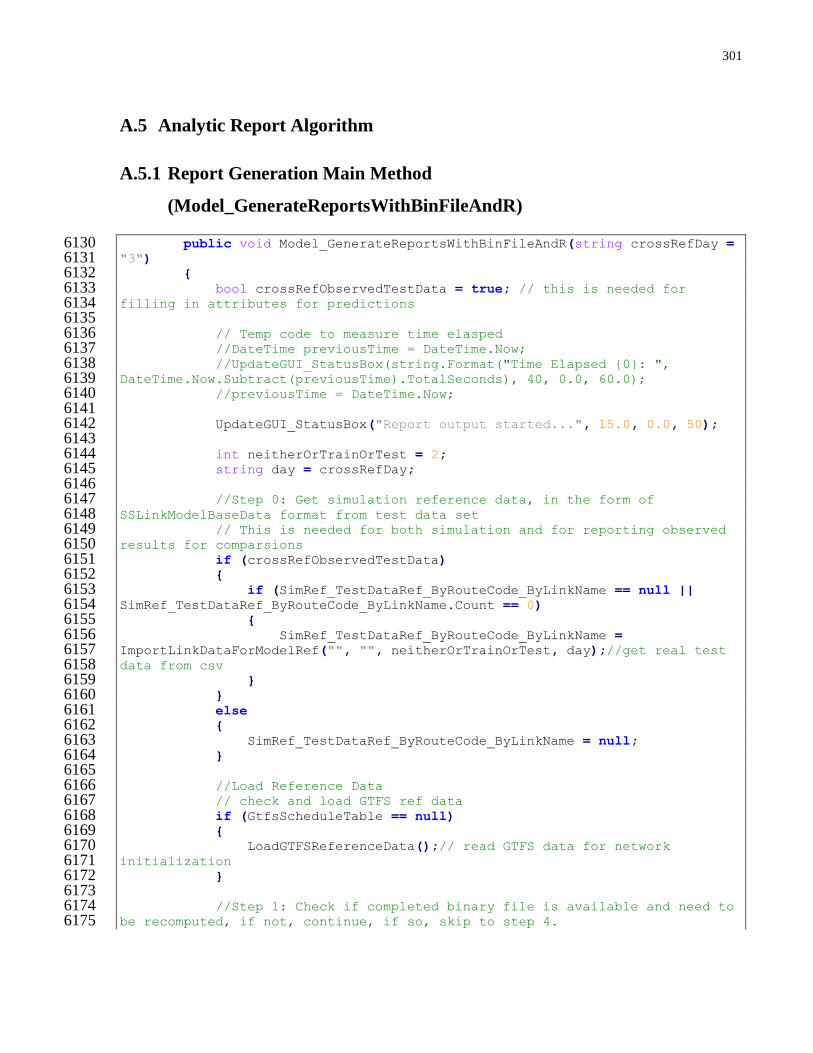
301
A.5 Analytic Report Algorithm
A.5.1 Report Generation Main Method
(Model_GenerateReportsWithBinFileAndR)
public void Model_GenerateReportsWithBinFileAndR(string crossRefDay = 6130 "3") 6131 { 6132 bool crossRefObservedTestData = true; // this is needed for 6133 filling in attributes for predictions 6134 6135 // Temp code to measure time elasped 6136 //DateTime previousTime = DateTime.Now; 6137 //UpdateGUI_StatusBox(string.Format("Time Elapsed {0}: ", 6138 DateTime.Now.Subtract(previousTime).TotalSeconds), 40, 0.0, 60.0); 6139 //previousTime = DateTime.Now; 6140 6141 UpdateGUI_StatusBox("Report output started...", 15.0, 0.0, 50); 6142 6143 int neitherOrTrainOrTest = 2; 6144 string day = crossRefDay; 6145 6146 //Step 0: Get simulation reference data, in the form of 6147 SSLinkModelBaseData format from test data set 6148 // This is needed for both simulation and for reporting observed 6149 results for comparsions 6150 if (crossRefObservedTestData) 6151 { 6152 if (SimRef_TestDataRef_ByRouteCode_ByLinkName == null || 6153 SimRef_TestDataRef_ByRouteCode_ByLinkName.Count == 0) 6154 { 6155 SimRef_TestDataRef_ByRouteCode_ByLinkName = 6156 ImportLinkDataForModelRef("", "", neitherOrTrainOrTest, day);//get real test 6157 data from csv 6158 } 6159 } 6160 else 6161 { 6162 SimRef_TestDataRef_ByRouteCode_ByLinkName = null; 6163 } 6164 6165 //Load Reference Data 6166 // check and load GTFS ref data 6167 if (GtfsScheduleTable == null) 6168 { 6169 LoadGTFSReferenceData();// read GTFS data for network 6170 initialization 6171 } 6172 6173 //Step 1: Check if completed binary file is available and need to 6174 be recomputed, if not, continue, if so, skip to step 4. 6175
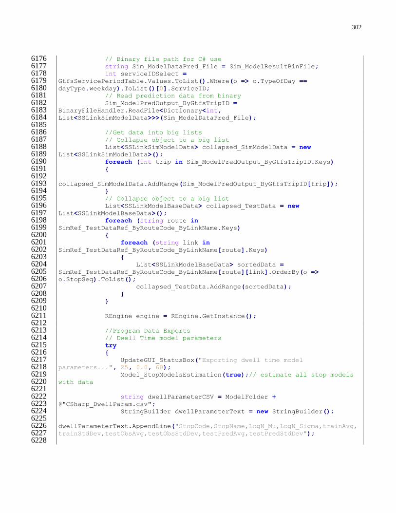
302
// Binary file path for C# use 6176 string Sim_ModelDataPred_File = Sim_ModelResultBinFile; 6177 int serviceIDSelect = 6178 GtfsServicePeriodTable.Values.ToList().Where(o => o.TypeOfDay == 6179 dayType.weekday).ToList()[0].ServiceID; 6180 // Read prediction data from binary 6181 Sim_ModelPredOutput_ByGtfsTripID = 6182 BinaryFileHandler.ReadFile<Dictionary<int, 6183 List<SSLinkSimModelData>>>(Sim_ModelDataPred_File); 6184 6185 //Get data into big lists 6186 // Collapse object to a big list 6187 List<SSLinkSimModelData> collapsed_SimModelData = new 6188 List<SSLinkSimModelData>(); 6189 foreach (int trip in Sim_ModelPredOutput_ByGtfsTripID.Keys) 6190 { 6191 6192 collapsed_SimModelData.AddRange(Sim_ModelPredOutput_ByGtfsTripID[trip]); 6193 } 6194 // Collapse object to a big list 6195 List<SSLinkModelBaseData> collapsed_TestData = new 6196 List<SSLinkModelBaseData>(); 6197 foreach (string route in 6198 SimRef_TestDataRef_ByRouteCode_ByLinkName.Keys) 6199 { 6200 foreach (string link in 6201 SimRef_TestDataRef_ByRouteCode_ByLinkName[route].Keys) 6202 { 6203 List<SSLinkModelBaseData> sortedData = 6204 SimRef_TestDataRef_ByRouteCode_ByLinkName[route][link].OrderBy(o => 6205 o.StopSeq).ToList(); 6206 collapsed_TestData.AddRange(sortedData); 6207 } 6208 } 6209 6210 REngine engine = REngine.GetInstance(); 6211 6212 //Program Data Exports 6213 // Dwell Time model parameters 6214 try 6215 { 6216 UpdateGUI_StatusBox("Exporting dwell time model 6217 parameters...", 25, 0.0, 60); 6218 Model_StopModelsEstimation(true);// estimate all stop models 6219 with data 6220 6221 string dwellParameterCSV = ModelFolder + 6222 @"CSharp_DwellParam.csv"; 6223 StringBuilder dwellParameterText = new StringBuilder(); 6224 6225 dwellParameterText.AppendLine("StopCode,StopName,LogN_Mu,LogN_Sigma,trainAvg,6226 trainStdDev,testObsAvg,testObsStdDev,testPredAvg,testPredStdDev"); 6227 6228
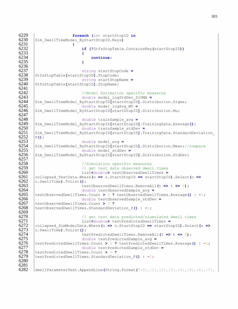
303
foreach (int startStopID in 6229 Sim_DwellTimeModel_ByStartStopID.Keys) 6230 { 6231 if (!GtfsStopTable.ContainsKey(startStopID)) 6232 { 6233 continue; 6234 } 6235 6236 string startStopCode = 6237 GtfsStopTable[startStopID].StopCode; 6238 string startStopName = 6239 GtfsStopTable[startStopID].StopName; 6240 6241 //Model Estimation specific measures 6242 double model_logStdDev_SIGMA = 6243 Sim_DwellTimeModel_ByStartStopID[startStopID].Distribution.Sigma; 6244 double model_logAvg_MU = 6245 Sim_DwellTimeModel_ByStartStopID[startStopID].Distribution.Mu; 6246 6247 double trainSample_avg = 6248 Sim_DwellTimeModel_ByStartStopID[startStopID].TrainingData.Average(); 6249 double trainSample_stdDev = 6250 Sim_DwellTimeModel_ByStartStopID[startStopID].TrainingData.StandardDeviation_6251 P(); 6252 double model_avg = 6253 Sim_DwellTimeModel_ByStartStopID[startStopID].Distribution.Mean;//compare 6254 double model_stdDev = 6255 Sim_DwellTimeModel_ByStartStopID[startStopID].Distribution.StdDev; 6256 6257 //Simulation specific measures 6258 // get test data observed dwell times 6259 List<double> testObservedDwellTimes = 6260 collapsed_TestData.Where(o => o.StartStopID == startStopID).Select(o => 6261 o.DwellTime).ToList(); 6262 testObservedDwellTimes.RemoveAll(t => t <= 0); 6263 double testObservedSample_avg = 6264 testObservedDwellTimes.Count > 3 ? testObservedDwellTimes.Average() : -1; 6265 double testObservedSample_stdDev = 6266 testObservedDwellTimes.Count > 3 ? 6267 testObservedDwellTimes.StandardDeviation_P() : -1; 6268 6269 // get test data predicted/siumulated dwell times 6270 List<double> testPredictedDwellTimes = 6271 collapsed_SimModelData.Where(o => o.StartStopID == startStopID).Select(o => 6272 o.DwellTime).ToList(); 6273 testPredictedDwellTimes.RemoveAll(t => t <= 0); 6274 double testPredictedSample_avg = 6275 testPredictedDwellTimes.Count > 3 ? testPredictedDwellTimes.Average() : -1; 6276 double testPredictedSample_stdDev = 6277 testPredictedDwellTimes.Count > 3 ? 6278 testPredictedDwellTimes.StandardDeviation_P() : -1; 6279 6280 6281 dwellParameterText.AppendLine(String.Format("{0},{1},{2},{3},{4},{5},{6},{7},6282

304
{8},{9}", startStopCode, startStopName, model_logAvg_MU, 6283 model_logStdDev_SIGMA, trainSample_avg, trainSample_stdDev, 6284 testObservedSample_avg, testObservedSample_stdDev, testPredictedSample_avg, 6285 testPredictedSample_stdDev)); 6286 } 6287 File.WriteAllText(dwellParameterCSV, 6288 dwellParameterText.ToString()); 6289 dwellParameterText.Clear(); 6290 } 6291 catch 6292 { 6293 UpdateGUI_StatusBox("Unexpected Error.", 25, 0.0, 0); 6294 } 6295 6296 //Analytics Reports 6297 // Time Distance Diagram for each schedule 6298 try 6299 { 6300 UpdateGUI_StatusBox("Producing time-distance diagrams...", 6301 40, 0.0, 280); 6302 string timeDistDiagFolder = ModelFolder + 6303 @"CSharp_TimeDistDiag\"; 6304 ExcelReports.CreateTimeDistDiagramReport(timeDistDiagFolder, 6305 collapsed_SimModelData, collapsed_TestData, GtfsStopTable, GtfsScheduleTable, 6306 GtfsRouteGroupTableByGroupID, serviceIDSelect); 6307 } 6308 catch 6309 { 6310 UpdateGUI_StatusBox("Unexpected Error.", 40, 0.0, 0); 6311 } 6312 6313 //Route Speed Reports 6314 try 6315 { 6316 UpdateGUI_StatusBox("Analyzing route speeds...", 60, 0.0, 6317 350); 6318 string routeReportFolder = ModelFolder + 6319 @"CSharp_RouteReport\"; 6320 ExcelReports.CreateRouteSpeedReport(routeReportFolder, 6321 collapsed_SimModelData, collapsed_TestData, GtfsStopTable, GtfsScheduleTable, 6322 GtfsRouteGroupTableByGroupID, serviceIDSelect, engine); 6323 } 6324 catch 6325 { 6326 UpdateGUI_StatusBox("Unexpected Error.", 60, 0.0, 0); 6327 } 6328 6329 //Stop Dwell Time Reports 6330 try 6331 { 6332 UpdateGUI_StatusBox("Analyzing stop dwell times...", 75, 0.0, 6333 90); 6334 string stopReportFolder = ModelFolder + 6335 @"CSharp_StopDwellReport\"; 6336

305
ExcelReports.CreateStopDwellReport(stopReportFolder, 6337 collapsed_SimModelData, collapsed_TestData, GtfsStopTable, GtfsScheduleTable, 6338 GtfsRouteGroupTableByGroupID, serviceIDSelect, engine); 6339 } 6340 catch 6341 { 6342 UpdateGUI_StatusBox("Unexpected Error.", 75, 0.0, 0); 6343 } 6344 6345 //Stop Delay Reports 6346 try 6347 { 6348 UpdateGUI_StatusBox("Analyzing stop delays...", 90, 0.0, 90); 6349 string stopReportFolder = ModelFolder + 6350 @"CSharp_StopDelayReport\"; 6351 ExcelReports.CreateStopDelayReport(stopReportFolder, 6352 collapsed_SimModelData, collapsed_TestData, GtfsStopTable, GtfsScheduleTable, 6353 GtfsRouteGroupTableByGroupID, serviceIDSelect, engine); 6354 } 6355 catch 6356 { 6357 UpdateGUI_StatusBox("Unexpected Error.", 90, 0.0, 0); 6358 } 6359 6360 //Clean Up 6361 Sim_ModelPredOutput_ByGtfsTripID.Clear(); 6362 SimRef_TestDataRef_ByRouteCode_ByLinkName.Clear(); 6363 UpdateGUI_StatusBox("Report output complete.", 100, 0.0, 0.0); 6364 // you should always dispose of the REngine properly. 6365 // After disposing of the engine, you cannot reinitialize nor 6366 reuse it 6367 engine.Dispose();//dispose at program exit 6368 } 6369 6370
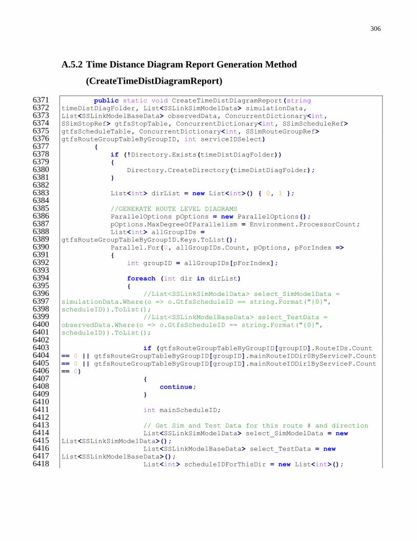
306
A.5.2 Time Distance Diagram Report Generation Method
(CreateTimeDistDiagramReport)
public static void CreateTimeDistDiagramReport(string 6371 timeDistDiagFolder, List<SSLinkSimModelData> simulationData, 6372 List<SSLinkModelBaseData> observedData, ConcurrentDictionary<int, 6373 SSimStopRef> gtfsStopTable, ConcurrentDictionary<int, SSimScheduleRef> 6374 gtfsScheduleTable, ConcurrentDictionary<int, SSimRouteGroupRef> 6375 gtfsRouteGroupTableByGroupID, int serviceIDSelect) 6376 { 6377 if (!Directory.Exists(timeDistDiagFolder)) 6378 { 6379 Directory.CreateDirectory(timeDistDiagFolder); 6380 } 6381 6382 List<int> dirList = new List<int>() { 0, 1 }; 6383 6384 //GENERATE ROUTE LEVEL DIAGRAMS 6385 ParallelOptions pOptions = new ParallelOptions(); 6386 pOptions.MaxDegreeOfParallelism = Environment.ProcessorCount; 6387 List<int> allGroupIDs = 6388 gtfsRouteGroupTableByGroupID.Keys.ToList(); 6389 Parallel.For(0, allGroupIDs.Count, pOptions, pForIndex => 6390 { 6391 int groupID = allGroupIDs[pForIndex]; 6392 6393 foreach (int dir in dirList) 6394 { 6395 //List<SSLinkSimModelData> select_SimModelData = 6396 simulationData.Where(o => o.GtfsScheduleID == string.Format("{0}", 6397 scheduleID)).ToList(); 6398 //List<SSLinkModelBaseData> select_TestData = 6399 observedData.Where(o => o.GtfsScheduleID == string.Format("{0}", 6400 scheduleID)).ToList(); 6401 6402 if (gtfsRouteGroupTableByGroupID[groupID].RouteIDs.Count 6403 == 0 || gtfsRouteGroupTableByGroupID[groupID].mainRouteIDDir0ByServiceP.Count 6404 == 0 || gtfsRouteGroupTableByGroupID[groupID].mainRouteIDDir1ByServiceP.Count 6405 == 0) 6406 { 6407 continue; 6408 } 6409 6410 int mainScheduleID; 6411 6412 // Get Sim and Test Data for this route # and direction 6413 List<SSLinkSimModelData> select_SimModelData = new 6414 List<SSLinkSimModelData>(); 6415 List<SSLinkModelBaseData> select_TestData = new 6416 List<SSLinkModelBaseData>(); 6417 List<int> scheduleIDForThisDir = new List<int>(); 6418

307
// NOTE: route ID = schedule ID, but =/= group ID or 6419 route code 6420 if (dir == 0) 6421 { 6422 6423 scheduleIDForThisDir.AddRange(gtfsRouteGroupTableByGroupID[groupID].mainRoute6424 IDDir0ByServiceP.Values.ToList()); 6425 6426 scheduleIDForThisDir.AddRange(gtfsRouteGroupTableByGroupID[groupID].subRouteI6427 DDir0.Select(o => o.Item3).ToList()); 6428 mainScheduleID = 6429 gtfsRouteGroupTableByGroupID[groupID].mainRouteIDDir0ByServiceP[serviceIDSele6430 ct]; 6431 } 6432 else 6433 { 6434 6435 scheduleIDForThisDir.AddRange(gtfsRouteGroupTableByGroupID[groupID].mainRoute6436 IDDir1ByServiceP.Values.ToList()); 6437 6438 scheduleIDForThisDir.AddRange(gtfsRouteGroupTableByGroupID[groupID].subRouteI6439 DDir1.Select(o => o.Item3).ToList()); 6440 mainScheduleID = 6441 gtfsRouteGroupTableByGroupID[groupID].mainRouteIDDir1ByServiceP[serviceIDSele6442 ct]; 6443 } 6444 foreach (int tempScheduleID in scheduleIDForThisDir) 6445 { 6446 select_SimModelData.AddRange(simulationData.Where(o 6447 => o.GtfsScheduleID == string.Format("{0}", tempScheduleID)).ToList()); 6448 select_TestData.AddRange(observedData.Where(o => 6449 o.GtfsScheduleID == string.Format("{0}", tempScheduleID)).ToList()); 6450 } 6451 6452 string mainScheduleStopString = string.Join(" ", 6453 gtfsScheduleTable[mainScheduleID].StopIDs); 6454 6455 if (select_SimModelData.Count > 0 && 6456 select_TestData.Count > 0) 6457 { 6458 string routeCode = 6459 gtfsRouteGroupTableByGroupID[groupID].RouteCode; 6460 6461 //gtfsRouteGroupTableByGroupID[gtfsScheduleTable[scheduleID].GroupID].RouteCo6462 de; 6463 string routeName = 6464 gtfsRouteGroupTableByGroupID[groupID].RouteName.Replace('/', ' '); 6465 6466 //gtfsRouteGroupTableByGroupID[gtfsScheduleTable[scheduleID].GroupID].RouteNa6467 me.Replace('/', ' '); 6468 //string routeTag = 6469 gtfsRouteGroupTableByGroupID[gtfsScheduleTable[scheduleID].GroupID].RouteInfo6470 [scheduleID].RouteTag; 6471
308
string routeHeading = 6472 gtfsRouteGroupTableByGroupID[groupID].RouteInfo[mainScheduleID].Name;//gtfsRo6473 uteGroupTableByGroupID[gtfsScheduleTable[scheduleID].GroupID].RouteInfo[sched6474 uleID].Name; 6475 string sheetLabel = string.Format("{0}-{1}-{2}", 6476 routeCode, groupID, dir); 6477 string chartTitle = string.Format("TIME DISTANCE 6478 DIAGRAM\n({0} {1} {2})", routeCode, routeName, routeHeading.Replace(" - ", 6479 "^").Split('^').Last()); 6480 string ExcelBookFilePath = timeDistDiagFolder + 6481 string.Format(@"TD_Diag_{0}-{1}-{2}.xlsx", routeCode, routeName, 6482 routeHeading.Replace(" - ", "^").Split('^').Last()); 6483 //string.Format(@"TD_Diag_{0}-{1}-{2}.xlsx", 6484 routeCode, routeName, scheduleID); 6485 6486 // Create the file using the FileInfo object 6487 //ExcelBookFilePath = ExcelBookFilePath.Replace('/', 6488 ' '); 6489 var file = new FileInfo(ExcelBookFilePath); 6490 6491 // Create the package and make sure you wrap it in a 6492 using statement 6493 using (var xlPackage = new ExcelPackage(file)) 6494 { 6495 //--- Simulation Data Workbook --- 6496 6497 // add a new worksheet to the empty workbook 6498 ExcelWorksheet worksheet_sim = 6499 xlPackage.Workbook.Worksheets.Add(string.Format("SimData_{0}", sheetLabel)); 6500 List<int> simSheetRowBreaks = new List<int>(); 6501 6502 // sort simulation data 6503 select_SimModelData = 6504 select_SimModelData.OrderBy(o => o.StopSeq).ToList(); 6505 select_SimModelData = 6506 select_SimModelData.OrderBy(o => o.GtfsTripID).ToList(); 6507 //double distFromStart = 0.0; 6508 6509 // populate simulation data 6510 int i = 1;//header 6511 int lastGTFSTripID = -1; 6512 // First of all the first row 6513 worksheet_sim.Cells[i, 1].Value = "Scheduled 6514 Path"; 6515 worksheet_sim.Cells[i, 2].Value = "Simulation 6516 Path"; 6517 worksheet_sim.Cells[i, 3].Value = "Distance From 6518 Start (km)"; 6519 worksheet_sim.Cells[i, 4].Value = "Link Dist 6520 (m)"; 6521 worksheet_sim.Cells[i, 5].Value = "StopCode"; 6522 worksheet_sim.Cells[i, 6].Value = "GTFSTripID"; 6523 i++; 6524

309
foreach (SSLinkSimModelData aRow in 6525 select_SimModelData) 6526 { 6527 if (aRow.GtfsTripID != lastGTFSTripID) 6528 { 6529 //distFromStart = aRow.LinkDist; 6530 //simSheetRowBreaks.Add(i);//insert blank 6531 row before this row here later 6532 i++;//add empty row to break the lines in 6533 the scatterplot 6534 lastGTFSTripID = aRow.GtfsTripID; 6535 } 6536 //else 6537 //{ 6538 // distFromStart += aRow.LinkDist; 6539 //} 6540 6541 int scheduleID = 6542 Convert.ToInt32(aRow.GtfsScheduleID); 6543 //check if it is best to use main schedule 6544 ID's stop distance or this schedule ID 6545 string scheduleStopString = string.Join(" ", 6546 gtfsScheduleTable[scheduleID].StopIDs); 6547 if 6548 (mainScheduleStopString.Contains(scheduleStopString)) 6549 { 6550 scheduleID = mainScheduleID; 6551 }//else keep the original scheduleID 6552 //Note: if really clean graph is desired, use 6553 only stops from schedules that are subset of the main schedule stops 6554 6555 int stopIndex = 6556 gtfsScheduleTable[scheduleID].StopIDs.IndexOf(aRow.StartStopID); 6557 double distFromStart = 6558 gtfsScheduleTable[scheduleID].StopDistances[stopIndex] / 1000; // to km 6559 string stopCode = 6560 gtfsStopTable[aRow.StartStopID].StopCode; 6561 6562 //arrival at stop 6563 worksheet_sim.Cells[i, 1].Value = 6564 aRow.StartStop_ScheduledArrivalTime; 6565 worksheet_sim.Cells[i, 2].Value = 6566 aRow.StartStop_SimArrivalTime; 6567 worksheet_sim.Cells[i, 3].Value = 6568 distFromStart; 6569 worksheet_sim.Cells[i, 4].Value = 6570 aRow.LinkDist; 6571 worksheet_sim.Cells[i, 5].Value = stopCode; 6572 worksheet_sim.Cells[i, 6].Value = 6573 aRow.GtfsTripID; 6574 i++; 6575 //departure from stop 6576 worksheet_sim.Cells[i, 1].Value = 6577 aRow.StartStop_ScheduledArrivalTime; 6578

310
TimeSpan StartStop_SimDepTime = 6579 TimeSpan.FromSeconds(aRow.StartStop_SimArrivalTime.TotalSeconds + 6580 aRow.DwellTime); 6581 worksheet_sim.Cells[i, 2].Value = 6582 StartStop_SimDepTime; 6583 worksheet_sim.Cells[i, 3].Value = 6584 distFromStart; 6585 worksheet_sim.Cells[i, 4].Value = 6586 aRow.LinkDist; 6587 worksheet_sim.Cells[i, 5].Value = stopCode; 6588 worksheet_sim.Cells[i, 6].Value = 6589 aRow.GtfsTripID; 6590 i++; 6591 }//end foreach 6592 int total_SimWorksheetRows = i; 6593 6594 //--- Observed Data Workbook --- 6595 // add a new worksheet to the empty workbook 6596 ExcelWorksheet worksheet_obs = 6597 xlPackage.Workbook.Worksheets.Add(string.Format("ObsData_{0}", sheetLabel)); 6598 List<int> obsSheetRowBreaks = new List<int>(); 6599 6600 // sort simulation data 6601 select_TestData = select_TestData.OrderBy(o => 6602 o.StopSeq).ToList(); 6603 select_TestData = select_TestData.OrderBy(o => 6604 o.GpsTripID).ToList(); 6605 //distFromStart = 0.0; 6606 6607 // populate simulation data 6608 int lastGPSTripID = -1; 6609 i = 1;//header 6610 // First of all the first row 6611 worksheet_obs.Cells[i, 1].Value = "Observed 6612 Path"; 6613 worksheet_obs.Cells[i, 2].Value = "Distance From 6614 Start (km)"; 6615 worksheet_obs.Cells[i, 3].Value = "Link Dist 6616 (m)"; 6617 worksheet_obs.Cells[i, 4].Value = "StopCode"; 6618 worksheet_obs.Cells[i, 5].Value = "GPSTripID"; 6619 i++; 6620 foreach (SSLinkModelBaseData aRow in 6621 select_TestData) 6622 { 6623 if (aRow.GpsTripID != lastGPSTripID) 6624 { 6625 //distFromStart = aRow.LinkDist; 6626 //obsSheetRowBreaks.Add(i);//insert blank 6627 row before this row here later 6628 i++;//add empty row to break the lines in 6629 the scatterplot 6630 lastGPSTripID = aRow.GpsTripID; 6631 } 6632

311
//else 6633 //{ 6634 // distFromStart += aRow.LinkDist; 6635 // 6636 6637 int scheduleID = 6638 Convert.ToInt32(aRow.GtfsScheduleID); 6639 //check if it is best to use main schedule 6640 ID's stop distance or this schedule ID 6641 string scheduleStopString = string.Join(" ", 6642 gtfsScheduleTable[scheduleID].StopIDs); 6643 if 6644 (mainScheduleStopString.Contains(scheduleStopString)) 6645 { 6646 scheduleID = mainScheduleID; 6647 }//else keep the original scheduleID 6648 //Note: if really clean graph is desired, use 6649 only stops from schedules that are subset of the main schedule stops 6650 6651 int stopIndex = 6652 gtfsScheduleTable[scheduleID].StopIDs.IndexOf(aRow.StartStopID); 6653 double distFromStart = 6654 gtfsScheduleTable[scheduleID].StopDistances[stopIndex] / 1000; // to km 6655 string stopCode = 6656 gtfsStopTable[aRow.StartStopID].StopCode; 6657 6658 //arrival at stop 6659 TimeSpan StartStop_ObsArrTime = 6660 TimeSpan.FromMinutes(aRow.Time_mins); 6661 worksheet_obs.Cells[i, 1].Value = 6662 StartStop_ObsArrTime; 6663 worksheet_obs.Cells[i, 2].Value = 6664 distFromStart; 6665 worksheet_obs.Cells[i, 3].Value = 6666 aRow.LinkDist; 6667 worksheet_obs.Cells[i, 4].Value = stopCode; 6668 worksheet_obs.Cells[i, 5].Value = 6669 aRow.GpsTripID; 6670 i++; 6671 //departure from stop 6672 TimeSpan StartStop_ObsDepTime = 6673 TimeSpan.FromSeconds(StartStop_ObsArrTime.TotalSeconds + aRow.DwellTime); 6674 worksheet_obs.Cells[i, 1].Value = 6675 StartStop_ObsDepTime; 6676 worksheet_obs.Cells[i, 2].Value = 6677 distFromStart; 6678 worksheet_obs.Cells[i, 3].Value = 6679 aRow.LinkDist; 6680 worksheet_obs.Cells[i, 4].Value = stopCode; 6681 worksheet_obs.Cells[i, 5].Value = 6682 aRow.GpsTripID; 6683 i++; 6684 }//end foreach 6685 int total_ObsWorksheetRows = i; 6686

312
6687 //--- Formatting Cell Number Format --- 6688 6689 worksheet_sim.Cells[string.Format("'{0}'!${1}${2}:{1}{3}", 6690 worksheet_sim.Name, "A", 2, 6691 total_SimWorksheetRows)].Style.Numberformat.Format = "HH:mm:ss"; 6692 6693 worksheet_sim.Cells[string.Format("'{0}'!${1}${2}:{1}{3}", 6694 worksheet_sim.Name, "B", 2, 6695 total_SimWorksheetRows)].Style.Numberformat.Format = "HH:mm:ss"; 6696 6697 worksheet_obs.Cells[string.Format("'{0}'!${1}${2}:{1}{3}", 6698 worksheet_obs.Name, "A", 2, 6699 total_ObsWorksheetRows)].Style.Numberformat.Format = "HH:mm:ss"; 6700 6701 //--- Time Distance Graph Workbook --- 6702 // add a new worksheet to the empty workbook 6703 ExcelWorksheet worksheet_Graph = 6704 xlPackage.Workbook.Worksheets.Add(string.Format("TimeDistDiag_{0}", 6705 sheetLabel)); 6706 6707 //Create Chart and Format it 6708 ExcelChart chart = 6709 (ExcelScatterChart)worksheet_Graph.Drawings.AddChart("TimeDistDiagChart", 6710 eChartType.XYScatterLinesNoMarkers); 6711 chart.Title.Text = string.Format("{0}", 6712 chartTitle); 6713 chart.Title.Font.Size = 16; 6714 chart.SetPosition(1, 0, 3, 0); 6715 chart.SetSize(900, 540);// ~("28 cm", "15 cm");// 6716 DPI: 166 //http://dpi.lv/ 6717 chart.DisplayBlanksAs = 6718 eDisplayBlanksAs.Gap;//need to display as Gap for proper visual 6719 6720 //chart.Style = eChartStyle.Style5; 6721 chart.YAxis.Title.Text = "Distance from Start 6722 (km)"; 6723 chart.YAxis.Title.Font.Size = 12; 6724 chart.XAxis.Title.Text = "Time (hh:mm:ss)"; 6725 chart.XAxis.Title.Font.Size = 12; 6726 chart.XAxis.MinValue = (double)6 / 24;//6am 6727 chart.XAxis.MaxValue = (double)9 / 24;//9am 6728 chart.XAxis.MajorUnit = (double)0.5 / 24; //30 6729 minutes 6730 chart.XAxis.MinorUnit = (double)0.25 / 24; //15 6731 minutes 6732 6733 // add schedule times 6734 string cellSelectString_Y = 6735 string.Format("'{0}'!${1}${2}:{1}{3}", worksheet_sim.Name, "C", 2, 6736 total_SimWorksheetRows); //Distance From Start (km) 6737 string cellSelectString_XSchedule = 6738 string.Format("'{0}'!${1}${2}:{1}{3}", worksheet_sim.Name, "A", 2, 6739 total_SimWorksheetRows); //Scheduled Path 6740
313
var ser1 = 6741 (ExcelChartSerie)(chart.Series.Add(worksheet_Graph.Cells[cellSelectString_Y], 6742 worksheet_Graph.Cells[cellSelectString_XSchedule])); 6743 ser1.Header = "Scheduled"; 6744 6745 // add observed times 6746 string cellSelectString_YObserved = 6747 string.Format("'{0}'!${1}${2}:${1}${3}", worksheet_obs.Name, "B", 2, 6748 total_ObsWorksheetRows); //Distance From Start (km) 6749 string cellSelectString_XObserved = 6750 string.Format("'{0}'!${1}${2}:${1}${3}", worksheet_obs.Name, "A", 2, 6751 total_ObsWorksheetRows); //Scheduled Path 6752 var ser2 = 6753 (ExcelChartSerie)(chart.Series.Add(worksheet_Graph.Cells[cellSelectString_YOb6754 served], worksheet_Graph.Cells[cellSelectString_XObserved])); 6755 ser2.Header = "Observed"; 6756 6757 // add simulation times 6758 //use cellSelectString_Y //Distance From Start 6759 (km) 6760 string cellSelectString_XSimulated = 6761 string.Format("'{0}'!${1}${2}:${1}${3}", worksheet_sim.Name, "B", 2, 6762 total_SimWorksheetRows); //Scheduled Path 6763 var ser3 = 6764 (ExcelChartSerie)(chart.Series.Add(worksheet_Graph.Cells[cellSelectString_Y], 6765 worksheet_Graph.Cells[cellSelectString_XSimulated])); 6766 ser3.Header = "Simulated"; 6767 6768 //// break series at every trip completion to 6769 have proper chart display of trips 6770 //// - for SimData sheet 6771 //foreach (int emptyRowNumInsert in 6772 simSheetRowBreaks) 6773 //{ 6774 // worksheet_sim.InsertRow(emptyRowNumInsert, 6775 1); 6776 //} 6777 //// - for ObsData sheet 6778 //foreach (int emptyRowNumInsert in 6779 obsSheetRowBreaks) 6780 //{ 6781 // worksheet_sim.InsertRow(emptyRowNumInsert, 6782 1); 6783 //} 6784 6785 // set graph sheet as selected 6786 6787 xlPackage.Workbook.Worksheets[worksheet_Graph.Name].View.TabSelected = true; 6788 6789 //--- Save The Entire Workbook --- 6790 xlPackage.Save(); 6791 }//end using 6792 }//end if count > 0 6793 }//end foreach dir 6794

314
//}//end foreach groupID 6795 }); 6796 }//end method 6797
6798

315
Appendix B Software Repository
The software program developed for this thesis can be found on two separate online code
repositories. Readers may request access to the program from the author via electronic mail at
bo.wen [at] alum [dot] utoronto [dot] ca. Alternatively, readers may request access to the
repositories by visiting the links below:
https://bitbucket.org/bowenwen/nexus.surfacesimulator
The first repository contains the Nexus Surface Simulator. The Nexus Surface Simulator is written
in C# and it consists of a set of tools that enables the data collection, data processing and model
estimation for transit data. Follow the instructions in “README.md” and “Installations.doc” to
set up your integrated developmental environment.
https://bitbucket.org/bowenwen/nexus.ssrtool
The second repository contains the R scripts used by the Nexus Surface Simulator package to
estimate models. Follow the instructions in “README.md” to set up the R scripts to be used by
the Nexus Surface Simulator.

316
Appendix C TRB Paper 2016
The attached paper was submitted to the 2016 Transportation Research Board Conference.

317
NEXUS SURFACE SIMULATOR FOR LARGE-SCALE TRANSIT SIMULATION
USING GPS AND GTFS DATA: FRAMEWORK AND TRAVEL TIME MODEL
Bo Wen Wen, B.A.Sc.
Department of Civil Engineering
University of Toronto
35 St. George Street, Toronto, ON, Canada M5S 1A4
Tel: 647-924-1996; Email: [email protected]
Siva Srikukenthiran, Ph.D.
Department of Civil Engineering
University of Toronto
35 St. George Street, Toronto, ON, Canada M5S 1A4
Tel: 416-978-5049; Email: [email protected]
Dennis Xu Wu
Department of Civil Engineering
University of Toronto
35 St. George Street, Toronto, ON, Canada M5S 1A4
Email: [email protected]
Prof. Amer Shalaby, Ph.D., P.Eng.
Department of Civil Engineering
University of Toronto
35 St. George Street, Toronto, ON, Canada M5S 1A4
Tel: 416-978-5907; Email: [email protected]
Word count: 5415 words text + 7 tables/figures x 250 words = 7165 words
2016-08-01
318
ABSTRACT
Transit network simulation is a critical planning and forecasting tool for assessing transit
performance, identifying operational shortcomings and evaluating potential service changes. In the
development of Nexus, an integrated transit network simulation platform, the surface transit arrival
patterns at major subway stations must be characterized. This study proposes Nexus Surface
Simulator, a computationally efficient large-scale transit network simulator using open data from
Automatic Data Collection Systems (ADCS) and General Transit Feed Specification (GTFS). A
modelling framework of the simulator and a first-stage prototype were developed. Using Support
Vector Regression (SVR), running time and dwell time models were estimated using GPS and
GTFS data. The SVR models replicated the observed conditions and produced acceptable root-
mean-square error measures. The results of the prototype simulator demonstrated the feasibility of
producing a large-scale travel time model to accurately represent the average weekday transit travel
conditions. Further developments of the simulator will include a vehicle simulation engine based
on the output conditions produced by the travel time model, which will then be integrated into the
Nexus platform.
Keywords: Public Transportation, Data and Information Technology, Planning and Forecasting

319
INTRODUCTION AND MOTIVATION
In many large cities around the world, public transit networks are operating near or at
capacity, leaving little room for absorbing service variation or disruptions. Currently, transit
agencies handle service irregularities and disruptions in an ad-hoc fashion. This is due to the lack
of analytical tools capable of realistically characterizing system performance under congested
conditions (due to capacity constraints and/or disruption incidents) and analyzing the impact of
response strategies. Nexus, an integrated crowd dynamics and transit network simulation platform
currently under development, enables the seamless interfacing of a rail simulator, a station and
pedestrian simulator, and a surface transit simulator to form a large-scale multimodal transit
network simulation (1). It overlays an agent-based framework to model passenger travel behaviour,
while permitting on-the-fly modifications to transit service operation (1). Nexus is designed to
perform capacity analysis of critical transit infrastructure, transit disruption scenario modelling
and analysis, and disruption response strategy assessment at the station, line and network levels.
The modelling of large-scale multimodal transit networks, such as those in Toronto,
Chicago and New York City, will require realistic representations of surface network operations
and their interactions with the rapid transit network in Nexus. Nexus currently uses a simplified
simulator of surface transit, with vehicles travelling according to scheduled times, but this does
not realistically represent the temporal variation of surface transit travel behaviour (1). Introducing
other vehicle modes and traffic signals would impose heavy data requirements, and would require
a traffic simulator which would greatly increase simulation time (1). As this may not be appropriate
for many situations, the objective of this study is to develop an alternate method where publicly
available transit data, such as global position systems (GPS) data of bus and streetcar movements,
are used to produce a statistical model of transit vehicle travel times between each vehicle stop.
State of Practice in Transit Modelling and Advances in Data
One of the major challenges in building a large-scale surface transit simulation is choosing
an appropriate modelling technique to realistically represent transit travel behaviour while
maintaining efficient computation. Macroscopic flow models incorporate aggregate variables such
as flow, density, and speed, but they are usually inadequate for modelling public transit because
they lack individual vehicle representations (2). At the other extreme, microsimulation software
can describe detailed interactions among transit vehicles, passengers, and traffic, which allows the
evaluation of complex public transit policies (3). However, in large networks, the simulation of
individual vehicles in microsimulation imposes high computational requirements (4). To overcome
this limitation, mesoscopic simulation models can be used since they do not explicitly model the
properties of individual vehicles such as position and velocity (5). Instead, they treat roadways as
queuing systems and track vehicle platoon flows (6). As such, mesoscopic simulation models can
produce stop-level statistics and are more suitable for large-scale transit applications.
Another major challenge in building a large-scale surface transit simulation is
characterizing the variation in transit vehicle travel. Recent studies have investigated the use of
artificial neural networks (ANN), support vector machines (SVM) and the k-nearest neighbour
algorithm (k-NN) to predict transit movement behaviour (7, 8, 9). It was found that SVM had the
strongest resistance to over-fitting (10). In addition, it demonstrated improved accuracy for
multiple route data (10). While previous studies have used statistical learning models to produce
travel time predictions for a limited number of routes, this study will use a statistical learning

320
model to develop a large-scale mesoscopic public transit network model with state-of-the-art GPS
and GTFS data.
Recent developments in public transit network modelling have been made possible by the
use of automatic data collection systems (ADCS) and general transit feed specification (GTFS)
(11). These advances in accessible public transit data have enabled modelling approaches that
require detailed network input data, such as new simulation methods based on a statistical learning
approach, as used in this study.
ADCS, such as automatic vehicle location systems (AVL), automatic passenger counting
systems (APC), and automatic fare collection systems (AFC), are capable of collecting real-time
data and archiving historical data (12). Bus locations collected by AVL-based GPS data are readily
available in real time. In contrast, passenger loading and passenger trip data, collected by APC and
AFC, respectively, are typically not available in real time (12). A large sample of detailed data with
measurable accuracy can be collected at a lower marginal cost by ADCS (12); this data can be used
to model transit vehicle travel and transit passenger demand.
GTFS is a standardized open data format for transit schedule data (13). Many transportation
modelling applications have been introduced as the result of the GTFS initiative. For example,
GTFS data have been used to build and update a large regional travel forecasting model (14). Map-
matching algorithms have been applied to GTFS data with GPS points from navigation to create a
multimodal transportation model (15). An intermodal shortest path algorithm has also been used
with GTFS data to develop a dynamic transit assignment model (16). Finally, transportation
simulation software packages including MATSim have used GTFS data to build microsimulation
model layouts (17).
Past studies have demonstrated the use of the ADCS and GTFS data in transit models. By
using both of these datasets, the transit travel patterns and transit network layout can be modelled
to evaluate transit network performance. The aim of this study is to develop a computationally
efficient surface transit simulator using these datasets which interfaces with the Nexus platform.
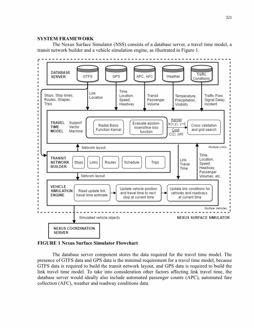
321
SYSTEM FRAMEWORK
The Nexus Surface Simulator (NSS) consists of a database server, a travel time model, a
transit network builder and a vehicle simulation engine, as illustrated in Figure 1.
FIGURE 1 Nexus Surface Simulator Flowchart
The database server component stores the data required for the travel time model. The
presence of GTFS data and GPS data is the minimal requirement for a travel time model, because
GTFS data is required to build the transit network layout, and GPS data is required to build the
link travel time model. To take into consideration other factors affecting link travel time, the
database server would ideally also include automated passenger counts (APC), automated fare
collection (AFC), weather and roadway conditions data.

322
The travel time model uses the processed data from the database server to estimate and
validate SVR models for link travel times. While the simulator can use a range of travel time
modelling methods such as ANN and k-NN, for the initial implementation of NSS, SVR has been
chosen due to its resistance to overfitting in comparison to other modelling methods (10). SVR’s
resistance to overfitting is largely attributed to the use of the v-fold cross validation procedure for
model training (18).
The network builder enables the construction of the transit network layout using GTFS
data. In particular, it converts processed GTFS data into data objects containing stop information,
link definitions, route layouts, route schedules and trip timetables. These data objects can be used
to automate the creation of large-scale surface transit networks, which can be quickly updated via
GTFS data when changes occur to the network. The network builder can also use this network
layout data to visually represent model information.
The final component, the vehicle simulation engine, simulates the movements of public
transit vehicles. The initial conditions for vehicle release are based on the starting stops and times
defined by the values stored in the GTFS trip tables. The SVR model is used to update the link
travel time periodically. The vehicle simulation engine uses this predicted link travel time to update
vehicle position, as well as the expected arrival time at downstream stops and stations. The updated
vehicle and link information is used in turn by the SVR model to compute a series of link travel
times for the next time step.
The conceptual design of the NSS also includes a connection interface to enable linking
the simulator to the Nexus coordination server. This allows the integration of surface transit
simulation with rail and pedestrian simulation on the Nexus platform for use in a broad range of
agent-based analyses of public transit systems (1).
METHODS
The first stage prototype of the NSS consists of a database server with GTFS and GPS data,
an SVR travel time model, and a transit network builder. Development of the first stage prototype
of the NSS involved four steps: data collection, data processing, model estimation and model
validation.
Case Study for the NSS Prototype
The objective of developing the first stage prototype was to test the accuracy of the SVR
travel time model for a large-scale surface transit network. The transit network chosen to build this
prototype was the Toronto Transit Commission (TTC) network, using available GTFS and GPS
data. The TTC network, operating within the City of Toronto, consists of 4 subway lines, 1 short
automated transit line, 11 streetcar lines, 140 bus lines, and over 10,000 transit stops. The TTC
surface transit system is well connected to the subway system with 148 out of 151 bus and streetcar
lines making 245 connections with the subway and the rapid transit line. The study period selected
for training the SVR model was from May 2, 2016 to May 6, 2016. A large-scale weekday morning
peak-period travel time model was developed for the TTC surface transit network for the study
period.

323
Data Collection
To collect data efficiently, web APIs were used to retrieve data from external data sources,
and store them within the NSS’s data server. This method allows for continuous training of the
travel time model with temporally varying data. The two sets of data used for the prototype NSS
were historical GTFS and GPS data. After determining the datasets required, the NSS retrieved
missing GTFS and GPS data for the study period. The GTFS and GPS data tables are summarized
in Table 1.
TABLE 1 Summary of database tables and variables in the GTFS and GPS data
The GTFS data contains schedule information for the transit service network. The GTFS
data for the TTC are updated around ten times per year. The updates to GTFS data correspond
closely to periodic service changes the TTC makes throughout the year. The GTFS data were
retrieved via the TransitFeeds website (19). The GTFS data are provided in the comma-separated
values (CSV) file format, containing information on transit service period, routes, shapes, stops,
324
stop times and trips. The GTFS data for the period between March 27, 2016 and May 7, 2016 were
used to construct the transit network structure for the NSS (20). The GTFS schedule information
in its raw CSV format was processed using a converter before being stored in a Nexus SQLite
database.
The GPS data were retrieved via the Connected Vehicles and Smart Transportation (CVST)
web API (21). These data contain vehicle information such as latitude, longitude, heading (bearing),
route information and vehicle identification, collected at 1 minute intervals. A set of AM peak
period (6:00 to 9:00) GPS data, from May 2, 2016 to May 6, 2016, was used as training data to
estimate the travel time model, while a set of testing data from April 25, 2016 to April 29, 2016,
AM peak period was used to validate the model. The latitude, longitude, heading, route information
and vehicle identification of the GPS points were sorted into vehicle trips and processed, as
detailed in Data Processing, before being stored in the SQLite database.
Data Limitations
No APC data was included in the prototype NSS due to the lack of network-wide data on
passenger counts for the TTC network. Although the deployment of AFC system on the TTC is
underway, the AFC system currently does not have network-wide availability (22). In addition, a
tap-on and -off AFC system is needed to fully characterize passenger trips from the AFC system
(11). Currently, the TTC has plans to implement tap-on and -off at subway stations by 2017 (23).
Finally, while weather and roadway incident data are available on Statistics Canada and Open Data
Toronto, respectively, they were not included in the first stage prototype because of the absence of
a web application program interface (API) implementation to retrieve these data efficiently.
Due to the unavailability of these data sources, a few assumptions on weather conditions,
traffic conditions and transit service quality were made in the travel time model. Firstly, due to the
exclusion of weather data, the GPS data was assumed to have been collected on days where there
would be minimal impact from weather on transit travel time. Secondly, the effects of incidents
and congestion were assumed to be implicit in the travel time model; in particular, the variation of
travel times across the modelling period was assumed to capture the background congestion level
of the modelling period. Finally, since a large part of the TTC network during peak hours has
frequent service of 10 minutes or less, headway variation between vehicles, as opposed to schedule
delay, was assumed to be a better indicator of transit service quality (24).
Data Processing
The raw data were processed into the appropriate formats and then stored in the data server,
allowing it to be used by the travel time model.
GTFS Data
Using a GTFS data converter, a network of routed vehicles with schedule stops and times
was built from a list of stops with a series of vehicle departure times. First, the converter read into
internal data structures all of the original GTFS data tables such as calendar, routes, shapes, stops,
stop times and trips. This allows the converter to organize the tables of trip segments and stop
departure times into series of vehicle blocks. Next, stop and route information were matched to
generate a schedule table. The schedule table defines a list of stops and distances between stops
with a unique schedule for each specific route and service period. Finally, the converter generated
325
a trip table with stop departure times linked to the schedule table. The schedule table provides the
network structure of the transit network by route and service period while the trip table provides a
detailed transit schedule. Together, they allow for the construction of network links, which are each
defined by a start stop and an end stop.
GPS Data
The GPS data were processed in order to determine the start and end stops and the estimated
speed and headway for each vehicle GPS point. First, after sorting each vehicle GPS points into
trips, the upstream (start) and downstream (end) stops were determined for the GPS point. This
was accomplished by identifying the link upon which the GPS point fell, based on the list of stops
and stop distances in the schedule table. The GPS points that did not fall on current segments in
the transit network were not considered in this study, including transit vehicles taking deadhead
trips or long detours. Next, the estimated speed and headway of the GPS points were calculated
based on the time and location of nearby GPS points. The estimated speed was calculated based
on the differences in time and distance between adjacent GPS points on the same trip, while the
estimated headway was approximated based on the differences in time between the subsequent
trips at approximately the same location. If the adjacent GPS points of a given trip did not change
position for more than 1 minute (the GPS data collection interval), the dwell times at transit stops
were determined. The time, speed, headway and vehicle identifications data for all the GPS points
were populated into their respective GTFS-based links.
Model Estimation using Support Vector Machines
The theoretical framework of the travel time model and the three basic components of SVR
machines are discussed.
Travel Time Model
The travel time model provides predictions of the running times between stops as well as
dwell times. The total travel time for a transit vehicle trip is the summation of these times across
the length of the route. As such, the SVR travel time model is a combination of a running time
model and a dwell time model, as shown in Equation 1.
𝑇𝑙,𝑏 = ∑ 𝑡𝑖,𝑙,𝑏𝑟𝑢𝑛𝑛𝑖𝑛𝑔
𝐼
𝑖=1
+ ∑ 𝑡𝑗.𝑙,𝑏𝑑𝑤𝑒𝑙𝑙
𝐽
𝑗=1
subject to 𝜉𝑖 ≥ 0 (1)
where 𝑇𝑙,𝑏 is the total travel time of a bus (b) along a specific route (l), 𝑡𝑖,𝑙,𝑏𝑟𝑢𝑛𝑛𝑖𝑛𝑔
is the
predicted running time at link i of a bus (b) along a specific route (l), and 𝑡𝑖.𝑙,𝑏𝑑𝑤𝑒𝑙𝑙 is the predicted
dwell time at stop j of a bus (b) along a specific route (l).
Soft Margin Hyperplane Optimization
SVMs are statistical learning models capable of classification and regression (25). They
are based on the idea of finding an optimal hyperplane that maximizes the separation or “margin”

326
between groups of data with different properties (18). The soft margin hyperplane which separates
data with minimum classification error is found using Equation 2 (26).
min1
2𝑤𝑇𝑤 + 𝐶 ∑ 𝜉𝑖
𝑙
𝑖=1
subject to 𝜉𝑖 ≥ 0 (2)
where 𝑤 is a normal vector to the hyperplane, C is the constant on the error terms
(regularization parameter), 𝑙 is the sample size, and 𝜉𝑖 are the estimation error terms (26).
Radial basis function kernel (RBF)
For linearly inseparable data, the kernel method is used to transform the data to higher
dimensions and then to classify the data in higher dimensions (25). To avoid the need to specify
the transformed data points explicitly, SVM uses a kernel function to compute the decision
boundaries (25). The kernel functional form and the kernel parameters determine the shape of the
hyperplane (25). A commonly used kernel function is the radial basis function (RBF) (see Equation
3). The RBF kernel has been chosen for its ability to handle nonlinear relations and its
computational efficiency with fewer hyperparameters (12).
𝐾(𝑥𝑖, 𝑥𝑗) = exp (−𝛾‖𝑥𝑖 − 𝑥𝑗‖2
)
subject to 𝛾 > 0 (3)
where 𝛾 is the kernel parameter; 𝑥𝑖 and 𝑥𝑗 are two feature vectors containing dependent
variables such as travel time on the link or dwell time at a stop, and independent variables such as
time value in 5-minute intervals and vehicle headway (18).
ε-insensitive loss function for SVR
To adapt SVM for regression, SVR uses an ε-insensitive error measure where low error
values are ignored while larger error contributes linearly to the absolute residual greater than a
constant ε (see Equation 4) (25). This makes the fitting less sensitive to outliers (25). The soft
margin hyperplane and kernel property are not limited to classification and have been demonstrated
in past studies to be integral to the properties of SVR (27). Furthermore, the kernel method for
SVR can avoid the need to evaluate a large set of functions to obtain error minimizations (25).
𝜉𝜀 = |𝑟| − 𝜀
subject to |𝑟| ≥ 𝜀 (4)
where 𝜀 is the loss function parameter and 𝑟 is the estimation error (25); this loss function
is applied to the error terms for Equation 1 of the SVR model estimation (27).
Parameter estimation and cross validation procedure
327
To estimate a SVR model based on RBF kernel and ε-insensitive loss functions, three
parameters need to be specified: the regularization parameter (𝐶), the kernel parameter (𝛾) and the
loss function parameter 𝜀. A v-fold cross validation procedure using a grid-search method was used
to find the most suitable set of 𝐶 and 𝛾 parameters. The v-fold cross validation procedure divides
training data into v number of subsets and trains the model sequentially by each subset (18). This
method of finding 𝐶 and 𝛾 prevents overfitting while minimizing the root-mean-square error of
the SVR model (18). A common 𝜀 value of 0.001 was used since it was reasonable to exclude very
small estimation errors (18). To implement SVR in the prototype NSS, LIBSVM library was used
to estimate the travel time model (28). Using the LIBSVM library, the SVR model was trained
with a set of link running times, time values in 5-minute intervals and vehicle headways. Using
the test set data with time values and vehicle headways as inputs, the trained model produced link
running time and dwell time predictions.
Validation of SVR Travel Time Model
After the final SVR models for link running time and dwell time were estimated, the trained
SVR models were validated against the test set data corresponding to the link or stop. This was
done by first using the trained SVR models to generate sets of predictions on link running time
and dwell time using the input test data. The sets of predictions were then compared against the
observed conditions in the test set data using the root-mean-square error (RMSE) measure.
RMSE = √1
𝑙∑(𝑓(𝑥𝑖) − 𝑦𝑖)2
𝑙
𝑖=1
subject to 𝑙 ≠ 0 (5)
where 𝑙 is the number of sample, 𝑓(𝑥𝑖) is the value of the predicted value, and 𝑦𝑖 is the
value of the observed value; the estimation error is 𝑟 = 𝑓(𝑥𝑖) − 𝑦𝑖 as shown in Equation 4.
RESULTS
The first stage prototype of the NSS produced a detailed travel time model for a large scale
transit network. The model training results and model validation results for link running times,
stop dwell times are presented in this section.
Results of link running time model
Using the route and stop information from the GTFS data, a complete set of links was
constructed to represent the entire TTC network. Using the GPS data on each of the links, a running
time model of each link was estimated using the training data set and validated using the test set
data. The running time model was able to replicate the slower travel speeds and lower travel times
in the Toronto downtown area, as well as the higher transit speeds outside the downtown core (see
Figure 2). The upper map shows the observed link travel times from the test set data, while the
lower map shows the predicted values for the same period.

328
FIGURE 2 Above: average of observed link running times for test set data. Below: average
of predicted link running times for test set data.

329
Validation of results
RMSE values were produced for the running time models (see Figure 3). The average
RMSE for link running times across the entire network was 0.60 min, which means on average, a
given link would provide a running time prediction of within 0.60 min of the observed running
time. While the RMSE for the Toronto downtown area was low (~1 min), some longer links in the
network showed poorer performance, such as links in the vicinity of York University and
Scarborough town centre areas (>2 min). A scatterplot of RMSE versus link length, as shown in
Figure 4, demonstrated a greater spread of RMSE with increasing link length (R2 = 0.60 for all
links, R2 = 0.1404 for link lengths less than 400m).
FIGURE 3 RMSE of link running times on the TTC network.
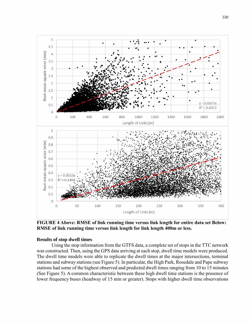
330
FIGURE 4 Above: RMSE of link running time versus link length for entire data set Below:
RMSE of link running time versus link length for link length 400m or less.
Results of stop dwell times
Using the stop information from the GTFS data, a complete set of stops in the TTC network
was constructed. Then, using the GPS data arriving at each stop, dwell time models were produced.
The dwell time models were able to replicate the dwell times at the major intersections, terminal
stations and subway stations (see Figure 5). In particular, the High Park, Rosedale and Pape subway
stations had some of the highest observed and predicted dwell times ranging from 10 to 15 minutes
(See Figure 5). A common characteristic between these high dwell time stations is the presence of
lower frequency buses (headway of 15 min or greater). Stops with higher dwell time observations

331
and predictions were usually terminal stops or subway stops. In contrast, lower dwell time
observations and predictions (<5 min) usually occurred at timed points or intersections with longer
than normal delays.
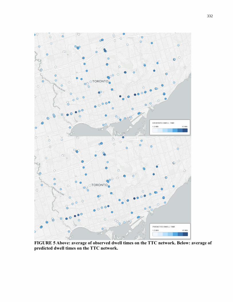
332
FIGURE 5 Above: average of observed dwell times on the TTC network. Below: average of
predicted dwell times on the TTC network.
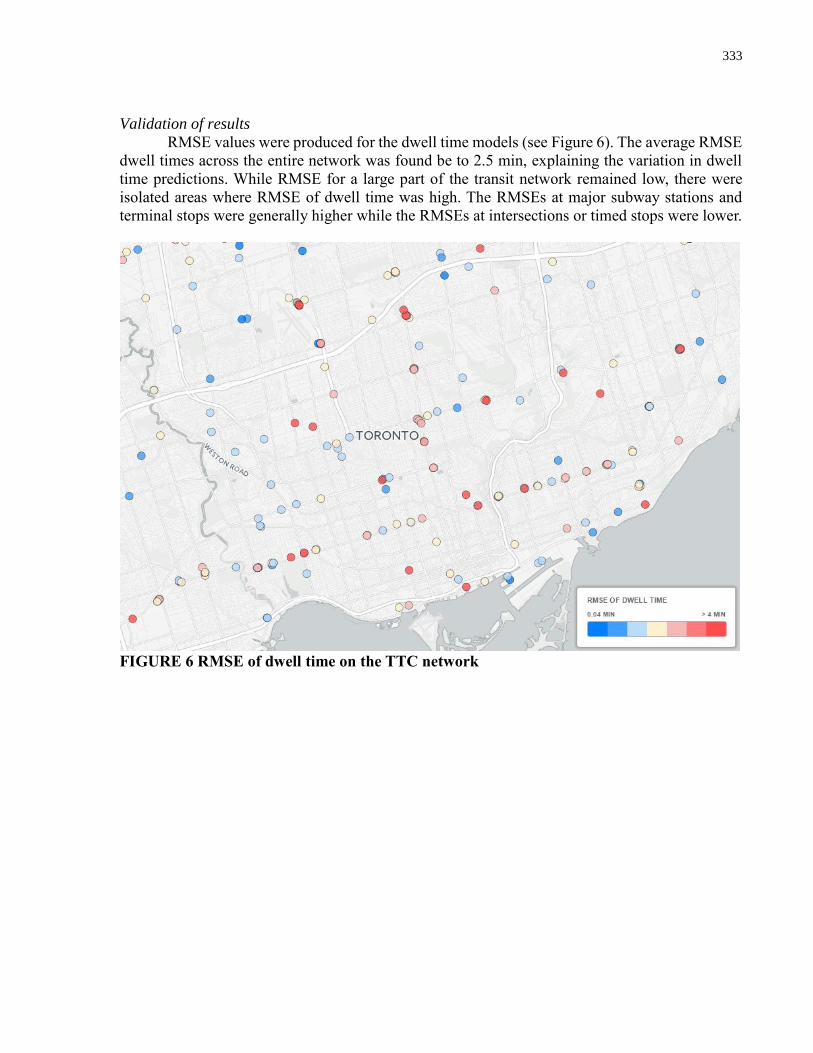
333
Validation of results
RMSE values were produced for the dwell time models (see Figure 6). The average RMSE
dwell times across the entire network was found be to 2.5 min, explaining the variation in dwell
time predictions. While RMSE for a large part of the transit network remained low, there were
isolated areas where RMSE of dwell time was high. The RMSEs at major subway stations and
terminal stops were generally higher while the RMSEs at intersections or timed stops were lower.
FIGURE 6 RMSE of dwell time on the TTC network
334
DISCUSSION AND CONCLUSION
This study presented the conceptual framework of a large-scale surface transit simulator to
be an eventual component of the Nexus integrated transit simulation platform. A first stage
prototype of the NSS, consisting of a data server, travel time model and a transit network builder,
was developed. The prototype NSS generated a detailed large-scale transit network, upon which a
travel time model was built. The travel time model used SVR to generate link running time and
stop dwell time models. The SVR models were able to replicate the observed conditions with
reasonable RMSE; however, the RMSE varied considerably across different links within the
network.
Two factors which may have influenced the performance of the running time models were
link length and roadway incidents. Longer link length was correlated with RMSE for the running
time models (R2 = 0.60 for all links). Longer links usually involve more turning movements and
intersection delays which were not captured and may have resulted in lower accuracy of predicted
link travel times. When examining shorter links where the stop distances are less than 400m (the
TTC criteria for the stop spacing is 300 to 500 m), the correlation between RMSE and link length
was less than that of all links (R2 = 0.60 for all links, R2 = 0.14 for link lengths less than 400m).
This implies that link distance is less of an influence on travel time for shorter links. Roadway
conditions including congestion and roadway incidents may influence transit travel times, but they
were not included in the running time model. Roadway conditions would be needed to improve
prediction performance.
The performance of the dwell time model may have been affected by the length of the GPS
polling time, lack of passenger loading data and exclusion of scheduled departure of the vehicles.
Dwell times shorter than the polling time of 60 seconds would not have been captured by the model.
This may have influenced the RMSE for the dwell time models. In addition, passenger boarding
and alighting data could improve the accuracy of the dwell time predictions, especially for non-
terminal bus stops. For terminal bus stations and subway stations, scheduled departure times of the
vehicle could improve dwell time predictions. Doing so will require the implementation of a
vehicle simulation engine where the arrival and departure times of a bus at a terminal station can
be tracked.
In the continued development of the NSS, a wider range of data, such as APC, AFC,
weather and traffic condition data, will be included in the data server to produce a more accurate
travel time model. The model could also be continuously trained with real-time transit data for
other applications such as real-time trip planning and real-time transit network management. Using
the updated travel time model, a vehicle simulation engine will then be developed to produce a
large-scale transit simulation network. Finally, the NSS will be integrated into the Nexus platform
where activity-based transit simulation will be performed to quantify multimodal transit
performances at the network-level.
335
ACKNOWLEDGEMENTS
The authors express gratitude to the resources provided to us by the Connected Vehicles
and Smart Transportation (CVST).
REFERENCES
1. Srikukenthiran, S., and A. Shalaby. Prototyping a Scalable Agent-based Modelling
Framework for Large-Scale Simulation of Crowd & Subway Network Dynamics.
Presented at the Conference on Advanced Systems in Public Transport, Santiago, Chile,
2012.
2. Spiliopoulou, A., M. Kontorinaki, and M. Papageor. Macroscopic traffic flow model
validation at congested freeway. Transportation Research Part C, Vol 41, 2014, pp. 18-29.
3. Fernandez, R., C. Cortes, and V. Burgos. Microscopic simulation of transit operations:
policy studies with the MISTRANSIT application programming interface. Transportation
Planning and Technology, Vol. 33, No. 2, 2010, pp. 157-176.
4. Cortes, C., L. Pages, and R. Jayakrishnan. Microsimulation of Flexible Transit System
Designs in Realistic Urban Networks. In Transportation Research Record: Journal of the
Transportation Research Board, No. 1923, Transportation Research Board of the National
Academies, Washington, D.C., 2005, pp. 153-163.
5. Toledo, T., O. Cats, W. Burghout, and H. Koutsopoulos. Mesoscopic simulation for transit
operations. Transportation Research Part C: Emerging Technologies, Vol. 18, No. 6, 2010,
pp. 896-908.
6. Cats, O., W. Burghout, T. Toledo, and H. Koutsopolous. Mesoscopic Modelling of Bus
Public Transportation. In Transportation Research Record: Journal of the Transportation
Research Board, No. 2188, Transportation Research Board of the National Academies,
Washington, D.C., 2010, pp. 9-18.
7. Chen, M., X. Liu, J. Xia, and S. Chien. A Dynamic Bus-Arrival Time Prediction Model
Based on APC Data. Computer-Aided Civil and Infrastructure Engineering, Vol. 19, No. 5,
2004, pp. 364–376.
8. Shalaby, A., and A. Farhan. Prediction Model of Bus Arrival and Departure Times Using
AVL and APC Data. Journal of Public Transportation, Vol. 7, No. 1, 2004, pp. 41-61.
9. Yu, B., Z. Yang, and B. Yao. Bus Arrival Time Prediction Using Support Vector Machines.
Journal of Intelligent Transportation Systems, Vol. 10, No. 4, 2006, pp. 151-158.
10. Yu, B., W. Lam, and M. L. Tam. Bus arrival time prediction at bus stop with multiple routes.
Transportation Research Part C: Emerging Technologies, Vol. 19, No. 6, 2011, pp. 1157-
1170.
11. Gaudette, P., R. Chapleau, and T. Spurr. Bus Network Microsimulation with GTFS and
Tap-in Only Smart Card Data. Presented at the 95th Annual Meeting of the Transportation
Research Board, Washington, D.C., 2016.
12. Munoz, J. C., and L. Paget-Seekins, eds. Restructuring Public Transport through Bus Rapid
Transit: An International and Interdisciplinary Perspective. Policy Press, Bristol, 2016.
13. Goldstein, B., and L. Dyson, eds. Beyond Transparency. Code for America Press, Portland,
2013.
336
14. Puchalsky, C., D. Joshi, and W. Scherr. Development of a Regional Forecasting Model
Based on Google Transit Feed. Presented at the 91st Annual Meeting of the Transportation
Research Board, Washington, D.C., 2012.
15. Perrine, K., A. Khani, and N. Ruiz-Juri. Map-Matching Algorithm for Applications in
Multimodal Transportation Network Modeling. In Transportation Research Record:
Journal of Transportation Research Board, No. 2537, Transportation Research Board of
the National Academies, Washington, D.C., 2015, pp. 62-70.
16. Khani, A., B. Bustillos, H. Noh, Y. Chiu, and M. Hickman. Modeling Transit and
Intermodal Tours in a Dynamic Multimodal Network. In Transportation Research Record:
Journal of the Transportation Research Board, No. 2467, Transportation Research Board
of the National Academies, Washington, D.C., 2014, pp. 21-29.
17. Nicolai, T. W., and K. Nagel. Integration of agent-based transport and land use, December
2013. http://svn.vsp.tu-berlin.de/repos/public-svn/publications/vspwp/2013/13-20/chapter
3-2_10dec2013.pdf. Accessed June 16, 2016.
18. Hsu, C.-W., C.-C. Chang, and C.-J. Lin. A Practical Guide to Support Vector Classification.
National Taiwan University, Taipei, 2016, pp. 1-16.
19. TransitFeeds. TTC GTFS – TransitFeeds. http://transitfeeds.com/p/ttc/33. Accessed April
30, 2016.
20. TransitFeeds. 19 March 2016 - TransitFeeds. https://transitfeeds.com/p/ttc/33/20160319.
Accessed May 20, 2016.
21. Connected Vehicles and Smart Transportation. CVST Live Traffic. http://portal.cvst.ca/.
Accessed June 21, 2016.
22. Hollis, R., and C. Upfold. Expanding Presto on TTC: Status Update.
http://www.metrolinx.com/en/docs/pdf/board_agenda/20160427/20160427_PRESTO_Im
plementation_Update_EN.pdf. Accessed July 16, 2016.
23. Borkwood, A. TTC Fare Policy. https://www.ttc.ca/About_the_TTC/Commission_reports
_and_information/Commission_meetings/2015/December_16/Reports/Presentation_Fare
_Policy_final.pdf. Accessed July 16, 2016.
24. Toronto Transit Commission. TTC introduces 10-minutes-or-better service on buses,
streetcars. https://www.ttc.ca/News/2015/June/0615_10min-service.jsp. Accessed July 17,
2016.
25. Hastie, T., R. Tibshirani, and J. Friedman. The Elements of Statistical Learning: Data
Mining, Inference, and Prediction. Springer, Stanford, 2008.
26. Cortes, C., and V. Vapnik. Support Vector Networks. Machine Learning, Vol. 20, 1995, pp.
273-297.
27. Smola, A. J., and B. Scholkopf. A Tutorial on Support Vector Regression.
http://www.svms.org/regression/SmSc98.pdf. Accessed June 22, 2016.
28. Chang, C.-C., and C.-J. Lin. LIBSVM: a library for support vector machines. ACM
Transactions on Intelligent Systems and Technology, Vol. 27, 2011, pp. 1-27.

337
Appendix D TransitData 2017 Abstract
The attached abstract was accepted and presented at the 2017 TransitData Conference.

338
AUTOMATIC MODELLING TOOL FOR ESTIMATING TRANSIT TRAVEL TIME TO
ENABLE SIMULATION OF LARGE-SCALE SURFACE TRANSIT NETWORKS
Bo Wen Wen, B.A.Sc.
Department of Civil Engineering
University of Toronto
35 St. George Street, Toronto, ON, Canada M5S 1A4
Tel: 647-924-1996; Email: [email protected]
Siva Srikukenthiran, Ph.D.
Department of Civil Engineering
University of Toronto
35 St. George Street, Toronto, ON, Canada M5S 1A4
Tel: 416-978-5049; Email: [email protected]
Prof. Amer Shalaby, Ph.D., P.Eng.
Department of Civil Engineering
University of Toronto
35 St. George Street, Toronto, ON, Canada M5S 1A4
Tel: 416-978-5907; Email: [email protected]
Introduction
Current microscopic simulation models can track the movements of transit vehicles but the
construction of these highly-detailed models is computationally expensive. On the other hand,
traditional macroscopic and mesoscopic models lack the ability to track the precise movements of
transit vehicles. Fortunately, with the advent of big data for transit systems, an efficient transit
travel simulation can be produced using a transit travel time model based on machine learning
algorithms. Previous studies on transit travel time models have used delay, traffic volume,
passenger demand and weather as key variables to predict bus travel times (Yu, et al., 2006; Chien,
et al., 2002). A comparison study on transit travel time models using support vector machine
(SVM), artificial neural networks (ANN), k-nearest neighbor (k-NN) and linear regression (LR)
found that SVM with data from multiple routes produced the most accurate travel time models
(Yu, et al., 2011). In particular, SVM showed greater resistance to the problem of over-fitting and
performed well with large data sets (Yu, et al., 2011). This paper presents an automatic modelling
tool that generates transit link travel time models using open data and SVM, with a case study on
the Toronto Transit Commission (TTC) network. The intended use of this modelling tool is to
enable the automatic development and updating of large-scale surface transit simulation models
using open data.
Methods
The automatic modelling tool collects Automatic Vehicle Location (AVL), General Transit Feed
Specification (GTFS), road restriction, signalized intersection and weather data, from online
sources, including NextBus API, Open Data Toronto and Open Weather Map API. During data
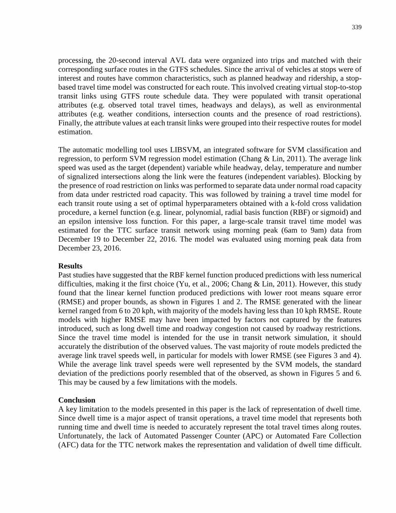
339
processing, the 20-second interval AVL data were organized into trips and matched with their
corresponding surface routes in the GTFS schedules. Since the arrival of vehicles at stops were of
interest and routes have common characteristics, such as planned headway and ridership, a stop-
based travel time model was constructed for each route. This involved creating virtual stop-to-stop
transit links using GTFS route schedule data. They were populated with transit operational
attributes (e.g. observed total travel times, headways and delays), as well as environmental
attributes (e.g. weather conditions, intersection counts and the presence of road restrictions).
Finally, the attribute values at each transit links were grouped into their respective routes for model
estimation.
The automatic modelling tool uses LIBSVM, an integrated software for SVM classification and
regression, to perform SVM regression model estimation (Chang & Lin, 2011). The average link
speed was used as the target (dependent) variable while headway, delay, temperature and number
of signalized intersections along the link were the features (independent variables). Blocking by
the presence of road restriction on links was performed to separate data under normal road capacity
from data under restricted road capacity. This was followed by training a travel time model for
each transit route using a set of optimal hyperparameters obtained with a k-fold cross validation
procedure, a kernel function (e.g. linear, polynomial, radial basis function (RBF) or sigmoid) and
an epsilon intensive loss function. For this paper, a large-scale transit travel time model was
estimated for the TTC surface transit network using morning peak (6am to 9am) data from
December 19 to December 22, 2016. The model was evaluated using morning peak data from
December 23, 2016.
Results
Past studies have suggested that the RBF kernel function produced predictions with less numerical
difficulties, making it the first choice (Yu, et al., 2006; Chang & Lin, 2011). However, this study
found that the linear kernel function produced predictions with lower root means square error
(RMSE) and proper bounds, as shown in Figures 1 and 2. The RMSE generated with the linear
kernel ranged from 6 to 20 kph, with majority of the models having less than 10 kph RMSE. Route
models with higher RMSE may have been impacted by factors not captured by the features
introduced, such as long dwell time and roadway congestion not caused by roadway restrictions.
Since the travel time model is intended for the use in transit network simulation, it should
accurately the distribution of the observed values. The vast majority of route models predicted the
average link travel speeds well, in particular for models with lower RMSE (see Figures 3 and 4).
While the average link travel speeds were well represented by the SVM models, the standard
deviation of the predictions poorly resembled that of the observed, as shown in Figures 5 and 6.
This may be caused by a few limitations with the models.
Conclusion
A key limitation to the models presented in this paper is the lack of representation of dwell time.
Since dwell time is a major aspect of transit operations, a travel time model that represents both
running time and dwell time is needed to accurately represent the total travel times along routes.
Unfortunately, the lack of Automated Passenger Counter (APC) or Automated Fare Collection
(AFC) data for the TTC network makes the representation and validation of dwell time difficult.
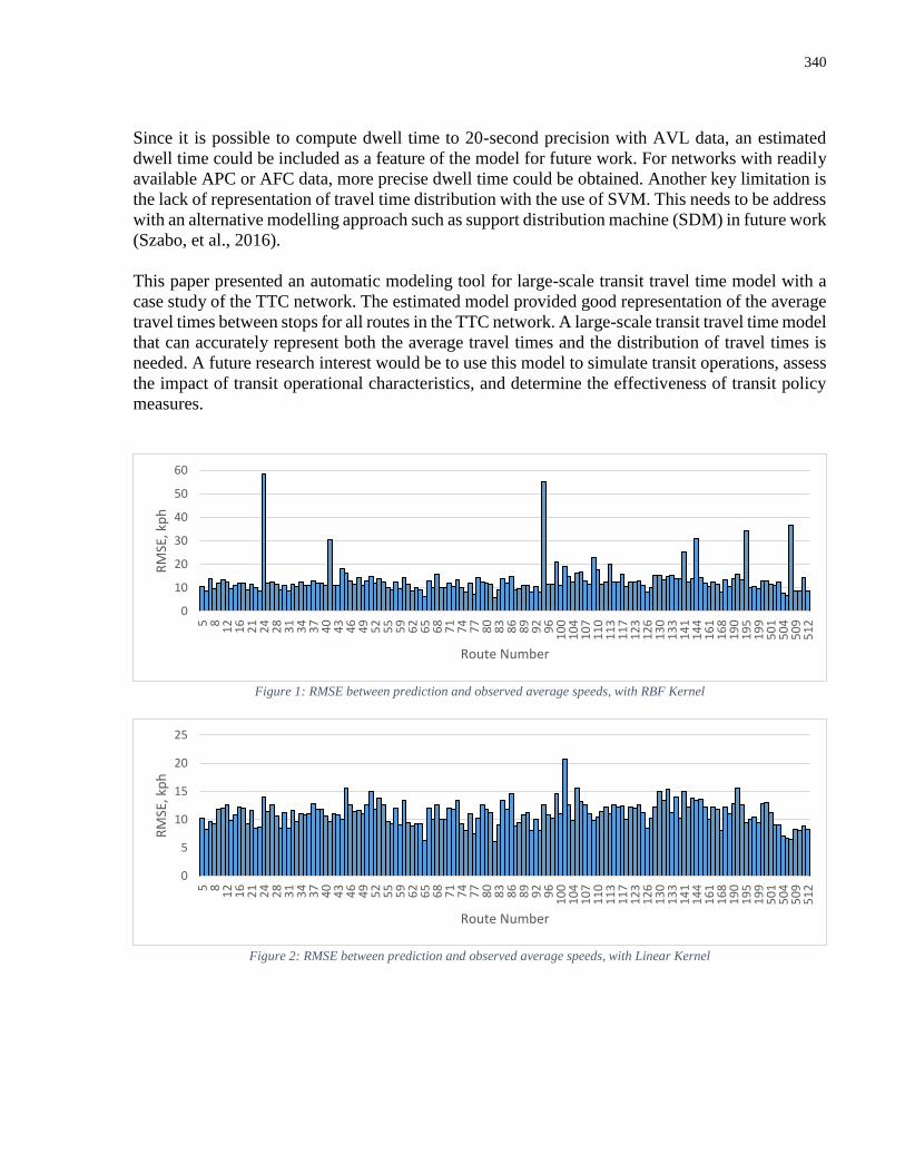
340
Since it is possible to compute dwell time to 20-second precision with AVL data, an estimated
dwell time could be included as a feature of the model for future work. For networks with readily
available APC or AFC data, more precise dwell time could be obtained. Another key limitation is
the lack of representation of travel time distribution with the use of SVM. This needs to be address
with an alternative modelling approach such as support distribution machine (SDM) in future work
(Szabo, et al., 2016).
This paper presented an automatic modeling tool for large-scale transit travel time model with a
case study of the TTC network. The estimated model provided good representation of the average
travel times between stops for all routes in the TTC network. A large-scale transit travel time model
that can accurately represent both the average travel times and the distribution of travel times is
needed. A future research interest would be to use this model to simulate transit operations, assess
the impact of transit operational characteristics, and determine the effectiveness of transit policy
measures.
Figure 1: RMSE between prediction and observed average speeds, with RBF Kernel
Figure 2: RMSE between prediction and observed average speeds, with Linear Kernel
0
10
20
30
40
50
60
5 81
21
62
12
42
83
13
43
74
04
34
64
95
25
55
96
26
56
87
17
47
78
08
38
68
99
29
61
00
10
41
07
11
01
13
11
71
23
12
61
30
13
31
41
14
41
61
16
81
90
19
51
99
50
15
04
50
95
12
RM
SE, k
ph
Route Number
0
5
10
15
20
25
5 81
21
62
12
42
83
13
43
74
04
34
64
95
25
55
96
26
56
87
17
47
78
08
38
68
99
29
61
00
10
41
07
11
01
13
11
71
23
12
61
30
13
31
41
14
41
61
16
81
90
19
51
99
50
15
04
50
95
12
RM
SE, k
ph
Route Number
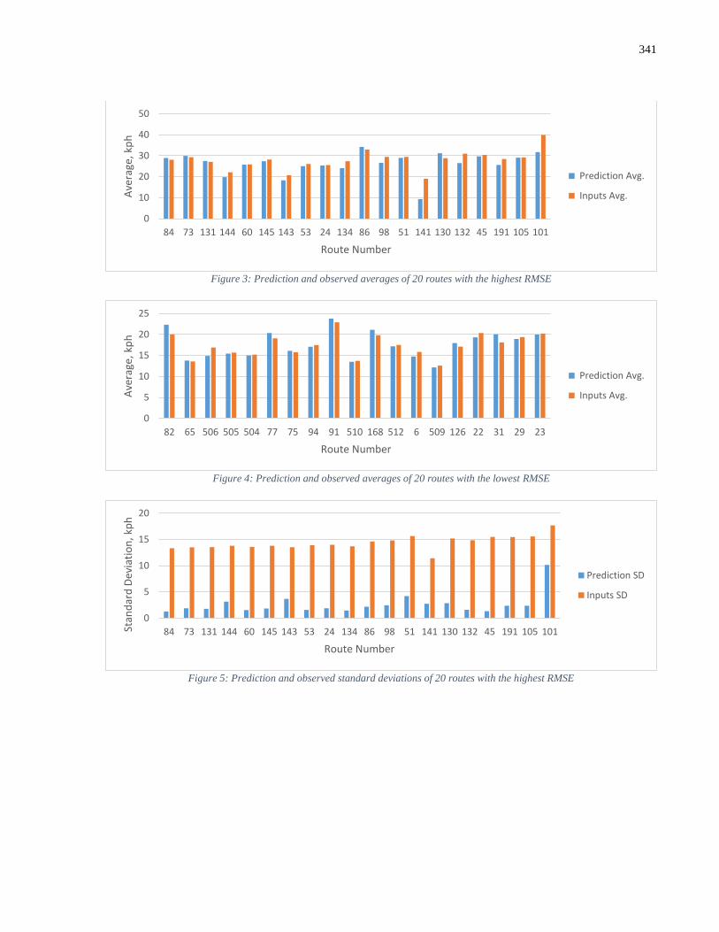
341
Figure 3: Prediction and observed averages of 20 routes with the highest RMSE
Figure 4: Prediction and observed averages of 20 routes with the lowest RMSE
Figure 5: Prediction and observed standard deviations of 20 routes with the highest RMSE
0
10
20
30
40
50
84 73 131 144 60 145 143 53 24 134 86 98 51 141 130 132 45 191 105 101
Ave
rage
, kp
h
Route Number
Prediction Avg.
Inputs Avg.
0
5
10
15
20
25
82 65 506 505 504 77 75 94 91 510 168 512 6 509 126 22 31 29 23
Ave
rage
, kp
h
Route Number
Prediction Avg.
Inputs Avg.
0
5
10
15
20
84 73 131 144 60 145 143 53 24 134 86 98 51 141 130 132 45 191 105 101Stan
dar
d D
evia
tio
n, k
ph
Route Number
Prediction SD
Inputs SD

342
Figure 6: Prediction and observed standard deviations of 20 routes with the lowest RMSE
Bibliography
Chang, C.-C. & Lin, C.-J., 2011. LIBSVM : a library for support vector machines. ACM
Transactions on Intelligent Systems and Technology, Volume 27, pp. 1-27.
Chien, S. I.-J., Ding, Y. & Wei, C., 2002. Dynamic Bus Arrival Time Prediction with Artificial
Neural Networks. Journal of Transportation Engineering, pp. 429-438.
Srikukenthiran, S., 2015. Integrated Microsimulation Modelling of Crowd and Subway Network
Dynamics For Disruption Management Support, Toronto, ON: Ph.D. dissertation, Graduate
Department of Civil Engineering, University of Toronto.
Szabo, Z., Sriperumbudur, B., Pocz, B. & Gretton, A., 2016. Learning Theory for Distribution
Regression. Journal of Machine Learning Research, 17(152), pp. 1-40.
Yu, B., Lam, W. & Tam, M. L., 2011. Bus arrival time prediction at bus stop with multiple routes.
Transportation Research Part C: Emerging Technologies, 19(6), pp. 1157-1170.
Yu, B., Yang, Z. & Yao, B., 2006. Bus Arrival Time Prediction Using Support Vector Machines.
Journal of Intelligent Transportation Systems, 10(4), pp. 151-158.
0
2
4
6
8
10
82 65 506 505 504 77 75 94 91 510 168 512 6 509 126 22 31 29 23Stan
dar
d D
evia
tio
n, k
ph
Route Number
Prediction SD
Inputs SD