trading in structured products: investor behavior and
TRANSCRIPT

TRADING IN STRUCTUREDPRODUCTS:
INVESTOR BEHAVIOR AND PRICING POLICIES
Zur Erlangung des akademischen Grades eines
Doktors der Wirtschaftswissenschaften
(Dr. rer. pol.)
von der Fakultät für
Wirtschaftswissenschaften
am Karlsruher Institut für Technologie (KIT)
genehmigte
DISSERTATION
von
Stephan Meyer
Tag der mündlichen Prüfung: 15. Januar 2014
Referent: Prof. Dr. Christof Weinhardt
Korreferent: Prof. Dr. Martin Ruckes
Karlsruhe, 2013


Abstract
For the last 10 years, we have witnessed a vast development of capital markets, in-troducing high frequency trading, bankruptcies of major institutions, and the estab-lishment of a market designed for small investors. For a long period of time, retailinvestors have solely been able to invest in stocks, bonds, or funds. Today, structuredproducts facilitate an advanced level of trading for retail investors allowing more so-phisticated trading strategies and short term speculation.
In my work I focus on structured products offering numerous risk-return varia-tions on a broad landscape of underlying assets. Compared to traditional investmentopportunities, structured products are often considered a more complex level of in-vesting, even allowing for betting on sideways and falling markets. However, withinthe last years, academics and regulators alike criticized the complexity of such prod-ucts, hiding risks from investors. Due to the fact that structured retail products areissued as bearer bonds, liquidity, i.e. buy and sell prices, for such products are exclu-sively provided by the issuing investment bank. Yet, while investors are now morethan ever capable of behaving like semi-professional traders, they could also be sub-ject of exploitation by issuers. An important question is therefore whether investorsput structured products to good use and whether issuers provide a fair and transpar-ent environment.
This thesis studies both issuing investment banks and investors in the marketfor structured products. I analyze whether issuers exploit investor ignorance andwhether investors benefit from this new market segment. My findings suggest thatissuers use their exclusive position to increase their rents on the expense of retailinvestors. The degree of exploitation varies strongly between product types and is-suers. Examining retail investor trades in short term speculation products revealsthat investors do not perform well in general and have, on average, no informationaladvantage. (Non-)profitability is driven to a large extent by transaction costs. Analyz-ing retail investor trades with respect to the risk incurred reveals a poor investmenton average. Investors expose themselves, i.e. their wealth, to great risk in order torealize potential profits.
Whether the regulator should step in to protect investors from losing money dueto their own misplaced actions and, to a smaller extent, the service charge in form ofhidden issuer fees remains beyond the scope of this thesis. Altogether, the findingsof this thesis suggest that regulators should pay close attention to the behavior ofparticipants in the market for structured products.
i

ii

Acknowledgements
This work would not have been possible without the support, encouragement, andadvice of several people. Foremost I would like to thank Prof. Dr. Christof Wein-hardt and Prof. Dr. Ryan Riordan for the opportunity to pursue my dissertation andproviding with me guidance when it was needed. I would also want to express mygratitude to my co-advisor Prof. Dr. Martin Ruckes and to the other members of thethesis committee, Prof. Dr. Thomas Setzer for providing me with support and fruitfuldiscussions, and Prof. Dr. Stefan Nickel, who has been so kind to guide me througha fair and insightful defense.
I am very grateful for the opportunity to work with my colleagues from the IISM inan excellent environment. Especially, I thank Dr. Martin Wagener for his continuoussupport and constructive critique throughout my thesis, Felix Fritz for being a greatco-author and office mate, Dr. Florian Teschner for his guidance, support, and thebeer, Philipp Ströhle for his way of making me laugh, Tobias Kranz for enduring mein his shelter, and Timm Teubner for his emotional and technical support. Besidesmy colleagues at the IISM, it is my pleasure to express special thanks to my fellowcolleague Sebastian Schroff who made my stay at the Boerse Stuttgart most enjoyableand for his fruitful cooperation up to this day.
Over the last years several friends made my life easier and helped me to face moreor less difficult times. Among many others, I would like to thank Johannes, Kai, Lya,Sebastian, Tim, Tobias, Walter, and Wolfgang.
I gratefully acknowledge that the research stay was supported by a scholarship ofthe Karlsruhe House of Young Scientists (KHYS).
Finally, I would like to thank my parents, Maria and Martin, and my sister Katha-rina for supporting and encouraging me throughout school, university, and my dis-sertation. Thank you.
iii

iv

Contents
List of Figures vi
List of Tables viii
1 Introduction 11.1 Motivation . . . . . . . . . . . . . . . . . . . . . . . . . . . . . . . . . . . 11.2 Research Outline . . . . . . . . . . . . . . . . . . . . . . . . . . . . . . . 51.3 Structure of the Thesis . . . . . . . . . . . . . . . . . . . . . . . . . . . . 7
2 The Universe of Structured Products 92.1 Product Design . . . . . . . . . . . . . . . . . . . . . . . . . . . . . . . . 92.2 Market Design and Trading Possibilities . . . . . . . . . . . . . . . . . . 112.3 Product Universe . . . . . . . . . . . . . . . . . . . . . . . . . . . . . . . 132.4 Regulation and Listing Fees . . . . . . . . . . . . . . . . . . . . . . . . . 202.5 Summary . . . . . . . . . . . . . . . . . . . . . . . . . . . . . . . . . . . . 32
3 Behavior of Participants 333.1 Issuer Behavior . . . . . . . . . . . . . . . . . . . . . . . . . . . . . . . . 333.2 Retail Investor Behavior . . . . . . . . . . . . . . . . . . . . . . . . . . . 423.3 Summary . . . . . . . . . . . . . . . . . . . . . . . . . . . . . . . . . . . . 52
4 Data and Methodology 534.1 Data Selection . . . . . . . . . . . . . . . . . . . . . . . . . . . . . . . . . 53
4.1.1 Thomson Reuters Quote Data . . . . . . . . . . . . . . . . . . . . 544.1.2 Stuttgart Stock Exchange Data . . . . . . . . . . . . . . . . . . . 544.1.3 Thomson Reuters News Data . . . . . . . . . . . . . . . . . . . . 57
4.2 Pricing Model . . . . . . . . . . . . . . . . . . . . . . . . . . . . . . . . . 604.2.1 (Practitioners) Black-Scholes Model . . . . . . . . . . . . . . . . 604.2.2 Black-Scholes and the Volatility Smile/Skew . . . . . . . . . . . 654.2.3 Implied Volatility Estimation . . . . . . . . . . . . . . . . . . . . 664.2.4 Limitations . . . . . . . . . . . . . . . . . . . . . . . . . . . . . . . 70
4.3 Summary . . . . . . . . . . . . . . . . . . . . . . . . . . . . . . . . . . . . 71
5 Investment Banks’ Price-Setting Behavior 735.1 Introduction . . . . . . . . . . . . . . . . . . . . . . . . . . . . . . . . . . 735.2 Research Questions . . . . . . . . . . . . . . . . . . . . . . . . . . . . . . 75
v

Contents
5.3 Sample Selection and Descriptive Statistics . . . . . . . . . . . . . . . . 775.4 Results . . . . . . . . . . . . . . . . . . . . . . . . . . . . . . . . . . . . . 81
5.4.1 Premiums of Investment Banks . . . . . . . . . . . . . . . . . . . 815.4.2 Intraday and Interday Effects . . . . . . . . . . . . . . . . . . . . 835.4.3 Risk and Demand Effects . . . . . . . . . . . . . . . . . . . . . . . 905.4.4 Premium Impact on Retail Investor Wealth . . . . . . . . . . . . 935.4.5 Complexity Effect . . . . . . . . . . . . . . . . . . . . . . . . . . . 98
5.5 Conclusion . . . . . . . . . . . . . . . . . . . . . . . . . . . . . . . . . . . 102
6 Retail Investors’ Trading Behavior 1056.1 Introduction . . . . . . . . . . . . . . . . . . . . . . . . . . . . . . . . . . 1056.2 Research Questions . . . . . . . . . . . . . . . . . . . . . . . . . . . . . . 1086.3 Sample Selection and Descriptive Statistics . . . . . . . . . . . . . . . . 109
6.3.1 Matched Sample . . . . . . . . . . . . . . . . . . . . . . . . . . . 1106.4 Results . . . . . . . . . . . . . . . . . . . . . . . . . . . . . . . . . . . . . 116
6.4.1 Profitability of Leveraged Trades . . . . . . . . . . . . . . . . . . 1166.4.2 Leverage, Volume, and Order Type . . . . . . . . . . . . . . . . . 1226.4.3 News Trading . . . . . . . . . . . . . . . . . . . . . . . . . . . . . 130
6.5 Conclusion . . . . . . . . . . . . . . . . . . . . . . . . . . . . . . . . . . . 134
7 Conclusion and Future Research 1377.1 Contributions . . . . . . . . . . . . . . . . . . . . . . . . . . . . . . . . . 1377.2 Regulatory Proposals and Implications . . . . . . . . . . . . . . . . . . . 139
7.2.1 Obligation to Provide Full Transparency . . . . . . . . . . . . . . 1397.2.2 Standardization . . . . . . . . . . . . . . . . . . . . . . . . . . . . 1407.2.3 Ban of Highly Complex Products . . . . . . . . . . . . . . . . . . 141
7.3 Outlook . . . . . . . . . . . . . . . . . . . . . . . . . . . . . . . . . . . . . 1427.4 Summary . . . . . . . . . . . . . . . . . . . . . . . . . . . . . . . . . . . . 144
A List of Abbreviations IA.1 List of Abbreviations . . . . . . . . . . . . . . . . . . . . . . . . . . . I
B German Product Classification III
C Sample Data - Thomson Reuters DataScope Tick History VII
D Sample Data - Stuttgart Stock Exchange Data XI
E Sample Data - Thomson Reuters News Data Description XVII
References XIX
vi

List of Figures
2.1 German Structured Products Monthly Outstanding Volume . . . . . . 142.2 Issuance Development in Germany . . . . . . . . . . . . . . . . . . . . . 152.3 Listings of Structured Products in Europe . . . . . . . . . . . . . . . . . 162.4 Turnover of Structured Products in Europe . . . . . . . . . . . . . . . . 172.5 Payoff: Discount Certificate . . . . . . . . . . . . . . . . . . . . . . . . . 182.6 Payoff: Bonus Certificate . . . . . . . . . . . . . . . . . . . . . . . . . . . 182.7 Payoff: Warrant . . . . . . . . . . . . . . . . . . . . . . . . . . . . . . . . 192.8 Payoff: Knock-out Warrant . . . . . . . . . . . . . . . . . . . . . . . . . . 192.9 Listing Fees Switzerland . . . . . . . . . . . . . . . . . . . . . . . . . . . 272.10 Listing Fees Switzerland For Less Than 2,000 Products . . . . . . . . . . 282.11 Listing Fees France . . . . . . . . . . . . . . . . . . . . . . . . . . . . . . 30
4.1 Black-Scholes Value of a Down-and-out Put Option . . . . . . . . . . . 644.2 Implied Volatility Skew . . . . . . . . . . . . . . . . . . . . . . . . . . . . 654.3 Implied Volatility Surface . . . . . . . . . . . . . . . . . . . . . . . . . . 674.4 Implied Volatility Over Time . . . . . . . . . . . . . . . . . . . . . . . . . 684.5 Euro Interbank Offered Rate Over Time . . . . . . . . . . . . . . . . . . 69
5.1 Number of Trades Throughout 2010 . . . . . . . . . . . . . . . . . . . . 785.2 Moneyness and Maturity Across Products . . . . . . . . . . . . . . . . . 805.3 Moneyness Across Products Over Time . . . . . . . . . . . . . . . . . . 815.4 Premium Across Products Over Time . . . . . . . . . . . . . . . . . . . . 835.5 Trading Frequency With Respect to Maturity . . . . . . . . . . . . . . . 855.6 Black-Scholes Value of a Down-and-out Put Option . . . . . . . . . . . 875.7 Average Intraday Premium and Volatility . . . . . . . . . . . . . . . . . 925.8 Relative Intraday Trade Frequency . . . . . . . . . . . . . . . . . . . . . 935.9 Relative Intraday Buy and Sell Frequency . . . . . . . . . . . . . . . . . 945.10 Substitute Algorithm Workflow . . . . . . . . . . . . . . . . . . . . . . . 101
6.1 News per Weekday on DAX30 Constituents April 2009 to February 2010 1146.2 Risk-Habitat - Stock . . . . . . . . . . . . . . . . . . . . . . . . . . . . . . 1226.3 Risk-Habitat - Index . . . . . . . . . . . . . . . . . . . . . . . . . . . . . . 1236.4 Invested Capital . . . . . . . . . . . . . . . . . . . . . . . . . . . . . . . . 1236.5 Leverage and Relative Spread . . . . . . . . . . . . . . . . . . . . . . . . 1246.6 News and Trades . . . . . . . . . . . . . . . . . . . . . . . . . . . . . . . 131
vii

List of Figures
7.1 Issuance Grid . . . . . . . . . . . . . . . . . . . . . . . . . . . . . . . . . 141
viii

List of Tables
2.1 National and International Regulation . . . . . . . . . . . . . . . . . . . 212.2 Listing Fees Germany . . . . . . . . . . . . . . . . . . . . . . . . . . . . . 262.3 Swiss Package Listing Fees . . . . . . . . . . . . . . . . . . . . . . . . . . 272.4 Listing Fees Austria . . . . . . . . . . . . . . . . . . . . . . . . . . . . . . 282.5 Listing Fees France . . . . . . . . . . . . . . . . . . . . . . . . . . . . . . 292.6 Listing Fees Sweden . . . . . . . . . . . . . . . . . . . . . . . . . . . . . . 302.7 Comparison of Listing Characteristics . . . . . . . . . . . . . . . . . . . 31
3.1 Related Work - Pricing of Structured Products . . . . . . . . . . . . . . . 403.2 Related Work - Retail Investor Performance . . . . . . . . . . . . . . . . 45
4.1 Stuttgart Stock Exchange - Master Data Example . . . . . . . . . . . . . 554.2 Stuttgart Stock Exchange - Order Flow Data Example . . . . . . . . . . 564.3 RNSE Data Sample . . . . . . . . . . . . . . . . . . . . . . . . . . . . . . 59
5.1 Descriptive Statistics - Trades . . . . . . . . . . . . . . . . . . . . . . . . 785.2 Descriptive Statistics - Quotes . . . . . . . . . . . . . . . . . . . . . . . . 795.3 Average Issuer Premiums and Spreads - Bonus Certificates . . . . . . . 825.4 Intraday and Interday Premium Shifts . . . . . . . . . . . . . . . . . . . 865.5 Intraday and Interday Premium Shifts - Issuer . . . . . . . . . . . . . . 885.6 Risk and Demand Effects . . . . . . . . . . . . . . . . . . . . . . . . . . . 915.7 Premium Impact on Retail Investors Wealth . . . . . . . . . . . . . . . . 975.8 Average Issuer Premiums - Discount and Capped Bonus Certificates . 1005.9 Substitutes . . . . . . . . . . . . . . . . . . . . . . . . . . . . . . . . . . . 103
6.1 Descriptive Statistics - Trades. . . . . . . . . . . . . . . . . . . . . . . . . 1126.2 Descriptive Statistics - Quotes . . . . . . . . . . . . . . . . . . . . . . . . 1136.3 Descriptive Statistics - News . . . . . . . . . . . . . . . . . . . . . . . . . 1156.4 Profitability . . . . . . . . . . . . . . . . . . . . . . . . . . . . . . . . . . . 1206.4 Profitability - continued . . . . . . . . . . . . . . . . . . . . . . . . . . . 1216.5 Profitability of Leveraged Trades . . . . . . . . . . . . . . . . . . . . . . 1266.5 Profitability of Leveraged Trades - continued . . . . . . . . . . . . . . . 1276.6 Volume, Leverage and Order Type . . . . . . . . . . . . . . . . . . . . . 1286.6 Volume, Leverage and Order Type - continued . . . . . . . . . . . . . . 1296.7 Retail Investor Trading Intensity Around News . . . . . . . . . . . . . . 1336.8 News Trading . . . . . . . . . . . . . . . . . . . . . . . . . . . . . . . . . 135
ix

List of Tables
B.1 German Classification for Structured Products . . . . . . . . . . . . IVB.1 German Classification for Structured Products - continued . . . . . V
C.1 Thomson Reuters DataScope Tick History - Intraday Sample . . . . VIIIC.2 Thomson Reuters DataScope Tick History - End-Of-Day Sample . . IX
D.1 Stuttgart Stock Exchange - Master Data Description . . . . . . . . . XIID.1 Stuttgart Stock Exchange - Master Data Description - continued . . XIIID.2 Stuttgart Stock Exchange - Order Data Description . . . . . . . . . . XIVD.3 Stuttgart Stock Exchange - Order Data Sample . . . . . . . . . . . . XV
E.1 Thomson Reuters News Data . . . . . . . . . . . . . . . . . . . . . . XVIII
x

Chapter 1
Introduction
”So, over the years we have often seen product design, marketing and sales processes
accentuate and distort the effects of human biases: teaser rates to take advantage of customer
inertia; bizarre insurance exclusions tucked away in the small print; terms and conditions for
financial products longer than Hamlet.”
Martin Wheatley (Chief Executive of the Financial Conduct Authority)
1.1 Motivation
ENGAGING in financial transactions is strongly linked to joy, regret, prosper-
ity, and social insecurity. No matter whether buying insurance, closing up a
mortgage, or investing in financial markets — to avoid poor decisions, consumers
either have to be very well informed and rational, or they put trust in their advi-
sors. On September 15, 2008 between 40,000 and 50,000 German investors lost more
than EUR 700 million due to underestimation and ignorance of existing risks.1 On
1Source: http://www.ftd.de/unternehmen/finanzdienstleister/:grundsatzurteil-lehman-anleger-bekommen-kein-geld-zurueck/60109511.html. Accessed07/06/2013. Numbers are only estimations by several German institutes. An older arti-cle from the NY Times quotes losses of ca. EUR 500 million for 60,000 investors: http://www.nytimes.com/2008/10/15/business/worldbusiness/15lehman.html?_r=0.Accessed 07/06/2013.
1

Chapter 1 Introduction
that day Lehman Brothers filed for bankruptcy.2 Lehman Brothers was an issuer of
structured products that were distributed by, among others, German banks such as
private banks, cooperative or savings banks. Structured (retail) products are bearer
bonds, which become worthless in case of a default of the issuer (default risk). They
are specifically designed to cater for the needs of retail investors. Investors with less
capital at hand, no access to derivatives, and limited knowledge of financial markets
(see, e.g., Ruf, 2011; Das, 2001). Structured products grant investors access to sophisti-
cated trading strategies and risk-return profiles for a broad range of different market
expectations. Although, the default risk is outlined in product descriptions, investors
were often not fully aware of it. Some relied blindly on their bank advisors and many
others did not comprehend the magnitude and probability of all involved risks.3 Var-
ious advised investors sued their banks on the basis of wrong consultation.4
Put simply, structured products are a well marketed cloak for the combination of
several financial securities, such as bonds and derivatives written on commodities,
currencies, indices, single or multiple stocks. This structuring of financial products in
form of bearer bonds leads to a distinct difference compared to regular stocks regard-
ing the price discovery. Prices for stocks are usually determined through the limit
order book at an exchange, consisting of orders of investors willing to buy or sell for
their submitted price (see, e.g., Harris, 2003). However, in case of structured products
issuers are in the exclusive position to set buy and sell prices for their own products
without any direct price competition. Investors cannot go short in a product. Thus,
the market design does not lead to efficient prices by its own. Consequently, issuers
are in a quasi-monopolistic position (Grünbichler and Wohlwend, 2005).
Among the most popular product types are bonus certificates. With bonus certifi-
cates investors participate in the underlying asset and are protected from losses up
to some extent. At the end of the life time investors receive a bonus payment if a
predefined lower threshold of the underlying asset has not been touched. Bonus cer-
tificates incorporate a barrier option. Barrier options start or cease to exist when the2Official press release: http://www.lehman.com/press/pdf_2008/091508_lbhi_chapter11_announce.pdf. Accessed 06/23/2013.
3See, for example, http://www.sueddeutsche.de/geld/anleger-und-die-lehman-pleite-geplatzte-traeume-1.691296. Accessed 08/20/2013.
4See, for example, http://www.welt.de/print/welt_kompakt/print_wirtschaft/article108749826/Ehepaar-erstreitet-nach-Lehman-Pleite-7-4-Millionen.html. Accessed 07/08/2013.
2

1.1 Motivation
underlying touches a predefined level. Although, the functionality is easy to under-
stand, the comprehension of an acceptable price is not. It requires experience with
asset pricing models, available data on the option market and the underlying market,
as well as the expertise to combine everything into a final price. Therefore, it seems
impossible for retail investors to actually look behind the marketing wall and decide
on a well-informed basis whether a product is fairly priced (Bethel and Ferrel, 2007).
Despite this lack of knowledge, German retail investors generate a total turnover of
about EUR 100 billion per year in structured products.5 Although, the bankruptcy of
Lehman Brothers represents a major setback for many investors, the German market
for structured products is still the most advanced and sophisticated market designed
for retail investors worldwide. From 2008 to 2013, the product universe has risen
from approximately 200,000 tradable products to more than one million products.
Retail investors can trade at low costs on all imaginable market movements and ex-
pectations. Every retail investor is able to act like a (semi-) professional trader and
can take an active part in his own investment strategies. Before the introduction of
this market segment, investors could solely buy funds, bonds, or stocks, which only
allowed for a limited playground of financial strategies.
However, new services and opportunities always come at a price. Due to the enor-
mous complexity of those products and the easy access to trading them, ordinary
retail investors are not capable of identifying whether the price of a product is ac-
curate and fair. This allows for fuzzy pricing strategies by issuers, which might aim
to exploit retail investors’ ignorance (Carlin, 2009; Carlin and Manso, 2010). Similar
to insurance contracts, where one usually does not know how much of the money is
spent on fees and premium for the sales person, retail investors have to think care-
fully whether costs and risks are acceptable.
Martin Wheatley is the head of the Financial Conduct Authority (FCA), a new
regulator in the UK that was formed in 2013 as a consequence of the last financial
crisis, aiming for a better protection of investors. Wheatley argues for a new era of
regulation taking into account behavioral biases of investors:
"You have to assume you don’t have rational consumers. Faced with complex
decisions or too much information, they default... They hide behind credit ratings
5See Section 2.3 for more information.
3

Chapter 1 Introduction
agencies or behind the promises that are given to them by the salesperson."6
The market for structured products facilitates every strategy an investor can imagine.
However, if this results in gambling and poor investment decisions it is up to the reg-
ulator to weigh opportunities and potential misuse of this market. Hens and Rieger
(2011) point out that the utility gain of structured products compared to the classic
approach of combining a risky asset (investing in the underlying) and a risk-free in-
vestment is negligible even given considerably low costs. They argue that behavioral
characteristics such as irrationality, loss-aversion, and misjudgment of probabilities
are likely explanations for the attractiveness of this market. The under-estimation of
probabilities is further supported by Rieger (2012) based on survey results. Based on
a survey of 757 German investors, Fischer (2007) finds that, besides diversification
and hedging of portfolios, gambling is a frequent motive for trading in structured
products. In addition, he finds that investors act irrationally, often failing at a proper
diversification or hedging strategy. Moreover, irrationality seems to increase with a
higher risk tolerance.
From a regulators’ perspective, this raises the question whether investors should
have the easy possibility to trade products they do not understand, and whether you
should regulate against all to protect some from being victimized? John Cochrane, a
renowned economist, thinks differently:
"Protecting" people because the bureaucracy just thinks it knows how to run
people’s lives better than they do. This used to be called aristocratic paternalism.
Now it’s defended by a misreading of behavioral economics.7
This thesis provides insights into the behavior of both issuers and investors in this
market, identifying possible exploitation by issuers and analyzing trading decisions
by investors. Combining both results provides a fundamental ground for future reg-
ulation.
6http://www.fca.org.uk/news/speeches/human-face-of-regulation. Accessed07/06/2013.
7http://johnhcochrane.blogspot.ca/2012/01/consumer-financial-protection-1984.html. Accessed 07/08/2013.
4

1.2 Research Outline
1.2 Research Outline
This thesis aims to explore characteristics and behavior of both issuers and investors
as well as their interaction in the German market for structured products. Issuers
have imposed upon themselves the obligation to set fair prices for their products
(Deutscher Derivate Verband, 2007). However, the last years have shown that in-
vestors and regulators alike become increasingly skeptical towards the intransparent
situation.8 Issuers do not provide any information on hidden fees, incorporated in
their products, as well as on their influencing factors (see, e.g., Bethel and Ferrel,
2007). Thus, investors have to belief that overall competition across similar existing
products and regulatory initiatives prevent them from being exploited.
Specifically, research contained in the work at hand is broken down into two major
research topics, addressing transparency and benefits of this market. Generally, in
markets that do not provide fully transparent information, investors may be subject
to exploitation by the market system and/or its dominating participants. However,
providing all (relevant) information is usually impossible. Thus, this dilemma raises
the question of the ideal level of information provision. The first research question
addresses this problem of (missing) transparency and, thus, the potential extent of
exploitation in the market for structured products:
Research Question 1. Do issuers exploit the ignorance of retail investors?
To shed light on this matter, I examine differences between theoretical prices, derived
from a standard asset pricing model and quoted issuer prices for several popular
product types. In the following, this difference is called premium or margin and
gives, in this raw form, an indication for the level of exploitation (Wilkens et al.,
2003; Wilkens and Stoimenov, 2007; Baule, 2011). I run a two-fold approach to de-
tect possible influencing factors on the included premium. First, I analyze whether
issuers systematically adjust their premiums during the day and over the life of a
structured product. Usually, structured products have a finite life time ranging from
a few months to several years. Continuously decreasing premiums result on aver-
8For example, the board of the International Organization of Securities Commissions (IOSCO) pub-lished in April 2013 a consultation paper which supports the discussion about the disclosure ofhidden fees and fair values of structured products. See http://www.iosco.org/library/pubdocs/pdf/IOSCOPD410.pdf. Accessed 06/26/2013.
5

Chapter 1 Introduction
age in higher buy prices and lower sell prices and, thus, support the assumption of
investor exploitation, as will be discussed in more detail in later chapters. Second,
based on retail investor trading data, I analyze whether issuers deliberately antici-
pate retail investor behavior to increase their profits.
Independent from hidden costs or possible unknown exploitation approaches by
issuers, it is still to be discussed whether retail investors make good use of this mar-
ket structure and resulting sophisticated trading strategies. This new market regime
allows, in contrast to traditional investing, to trade on a (semi-) professional level.
Traditionally, retail investments have been focused on retirement portfolios and thus
long-term investments. Retail investors bought funds, stocks, and bonds aiming for
a higher average long-term profit compared to risk-free assets. Today, retail investors
can enter positions for only minutes and exit with huge profits, something alike has
never been possible this easy before. This leads to the second overall research ques-
tion, focusing on this market from the perspective of overall economic benefit for
retail investors:
Research Question 2. Is trading in structured products beneficial for retail
investors’ wealth?
In recent years a major part of trading volume in the German market for structured
products has been generated in leverage products, i.e. products that participate dis-
proportionately in the underlying asset. Leverage products are not suitable for long
holding periods, but for speculation in the short term (Entrop et al., 2011). So far it
is unknown whether retail investors use this new opportunity to incorporate private
information in the market or if they merely trade for sensation seeking and entertain-
ment. Studies such as Dorn et al. (2012) show that some groups of investors tend to
substitute gambling with trading lottery-like stocks.
Altogether, the above research questions aim to provide a comprehensive picture
of all participating parties in this innovative market, providing in-depth analyses of
both, issuers and investors with respect to the regulatory environment.
6

1.3 Structure of the Thesis
1.3 Structure of the Thesis
The remainder of this thesis is organized as follows. Chapter 2 provides a solid back-
ground on the market for structured products in Germany, including a description
of the market design, the most popular product types, market statistics for several
European countries, and an overview of the current regulatory environment. Chap-
ter 3 provides a literature overview regarding the behavior of market participants,
i.e. issuers and investors. The first part summarizes empirical and theoretical stud-
ies focusing on the pricing of structured products in Germany and other compara-
ble markets. Second, literature regarding retail investor trading and its outcomes on
performance and order aggressiveness are presented. Additionally, I present well-
known decision-making failures and behavioral biases, which are relevant for this
thesis. The subsequent chapter presents information on used data sources as well as
a detailed description and discussion of limitations of the methodological approach
used to derive prices for structured products. Chapter 5 analyzes the price-setting be-
havior of German issuers with respect to several influencing parameters and its effect
on retail investor wealth.9 Chapter 6 examines retail investor behavior, focusing on
leverage structured products.10 It aims to study how well informed retail investors
are from different perspectives. Chapter 7 summarizes the key contributions of this
thesis, discusses regulatory implications, and outlines promising related topics for
future research.
9Parts of this chapter are joint work with Felix Fritz (Fritz and Meyer, 2012) and have been presentedat the 20th Finance Forum (Oviedo, Spain) and the Stuttgart Stock Exchange Research Colloquium2012 (Stuttgart, Germany). It has been invited for presentation at the 25th Australasian Finance& Banking Conference (Sydney, Australia), the 2012 Auckland Finance Meeting (Auckland, NewZealand), the International Mathematical Finance Conference (Miami, USA), and the 49th AnnualMeeting of the Eastern Finance Association (St. Pete Beach, United States). Some parts of this chap-ter are based on a joint working paper with Ryan Riordan (Meyer and Riordan, 2013). Addition-ally, an overview article based on some of the results contained in this chapter has been published(Meyer et al., 2013).
10This chapter is based on a joint paper with my colleagues Sebastian Schroff and Christof Weinhardt(Meyer et al., 2013). A previous version was circulated under the title "Lottery Losses of RetailInvestors". Results have been presented at the 22nd European Financial Management Association(EFMA) conference (Reading, UK) and at the 30th International French Finance Association Confer-ence (AFFI) (Lyon, France). The paper is forthcoming in Financial Markets and Portfolio Management.
7

Chapter 1 Introduction
8

Chapter 2
The Universe of Structured Products
THIS chapter provides a solid background on characteristics of structured prod-
ucts and the regulatory environment. Taken together, it builds the foundation
for all upcoming analyses that particularly focus on the German market for struc-
tured products, which is among the most advanced markets worldwide. I describe
the German market structure, focusing on design aspects of tradable securities (Sec-
tion 2.1) and of the market itself (Section 2.2). Section 2.3 provides details on popular
product types with respect to their risk and investor target group as well as descrip-
tive statistics for both, the German and other European markets. Section 2.4 presents
information on regulatory aspects for the German market as well as its differences to
other European markets with respect to listing fees.
2.1 Product Design
A structured retail product is a bearer bond issued by an investment bank.1 Simi-
lar expressions are bank-issued product or securitized derivative. Although, there
is no uniform definition of a structured product across exchanges or countries, they
have a basic feature in common: they are all built through a combination of funda-
mental financial securities, such as derivatives, equities, indices, bonds, currencies,
1A bearer bond is a "bond not registered in the name of an owner and that therefore belongs towhoever holds the bearer certificate. Dividends or interest payments are claimed using couponsattached to the certificate, which is transferable and negotiable without endorsement." (Finan-cial Times Lexicon, http://lexicon.ft.com/Term?term=bearer-stock/bond. Accessed08/07/2013.)
9

Chapter 2 The Universe of Structured Products
or commodities. The Federation of European Securities Exchanges (FESE) defines a
structured product as a "tradable financial instrument designed to meet specific in-
vestor needs and to respond to different investment strategies, by incorporating spe-
cial, non-standard features."2 The payoff at maturity, i.e. at the end of the life time of
the product, is defined through exact formulas published by issuers. Although, such
formulas are based mainly on the performance of the underlying asset, several more
exotic conditions are sometimes included. This includes conditions and features such
as lookback, dual currency, ranges, targets, moving barriers, accrual, podium, or cap.
Each of them increases the complexity of the structured product and the return for-
mula. Thus, the payoff profile gives the impression of a ’constructed’ return.
Structured products fill the gap for investors with partly insufficient funds, knowl-
edge, and access possibilities to create such complex security combinations them-
selves. Therefore, primary customers for structured products are retail investors
(Bethel and Ferrel, 2007). Besides not having the expertise to combine fundamen-
tal financial securities to a more complex product in a successful manner, a reason for
retail investors to invest into a structured product, instead of a direct investment in
the underlying basic components, is the reduced transaction costs. For example, in-
vesting in products with an index as underlying is cheaper than manually duplicating
the index by buying all constituents. Additionally, share prices of structured products
are reduced to an investor friendly level, which allows for small investments. This is
achieved by introducing a subscription ratio. For example, a subscription ratio of 1:10
for a structured product means that investors participate to the tenth of the return of
the underlying asset. In volume terms, assume the price of the structured product to
be EUR 10 with a subscription ratio of 1:10, and the underlying asset price to be EUR
100. If the price of the underlying increases by EUR 10 the price of the structured
product increases by EUR 1.
To achieve payoff profiles similar to structured products, investors have to be able
to trade derivatives. However, retail investors usually have no access to option ex-
changes through their broker. Therefore, structured products allow for sophisticated
trading strategies and provide a relatively new investment opportunity besides tradi-
2This quote is taken from the FESE methodology which can be found at: http://www.fese.be/_lib/files/FESE_Statistics-Methodology_5_2_January10_FINAL.pdf. Accessed05/10/2013.
10

2.2 Market Design and Trading Possibilities
tional investments in stocks, funds, or bonds. With the possibility to indirectly enter
a short position in an underlying, structured products can serve as a hedging instru-
ment for retail investor portfolios. A wide range of product characteristics allows in-
vestors to find a product, which perfectly matches their risk-return profile. Structured
products are issued in a variety of different combinations and maturities. In case of a
stock as underlying, the investor has no rights (e.g., voting rights) whatsoever regard-
ing the underlying and usually has to forego occurring dividend payments. Issuers
withhold dividend payments and often adapt product prices to the expectation of
future dividend payments.
Due to the legal structure of structured products, it is not subject of any deposit
protection. Therefore, invested money bears the risk of a total loss in case of a
bankruptcy of the issuing investment bank. In 2008, this case became true with the
collapse of Lehman Brothers.3
2.2 Market Design and Trading Possibilities
In Germany, structured products can be traded in two ways. First, via an over-the-
counter (OTC) platform of a bank or broker and, second, via market segments of
regulated exchanges such as Scoach4 in Frankfurt or EUWAX in Stuttgart. Retail in-
vestors do not need a trading license or proof of specific knowledge to trade struc-
tured products. Nevertheless, regulation requires companies to enquire information
about the securities-related knowledge, experience, investment strategy, and finan-
cial background of customers to recommend suitable financial instruments. There-
fore, investors have to provide information regarding their investment skills upon
registration with their broker. This survey is designed in a simple manner, often lim-
ited to the question whether they have already traded different security groups. In
addition, investors are required to confirm that they are aware of the risks involved
before they are allowed to submit an order with their broker. There is no additional
3Source: e.g., http://www.nytimes.com/2008/10/15/business/worldbusiness/15lehman.html?_r=0. Accessed 07/06/2013.
4In November 2013 Deutsche Boerse and SIX have started to go separate ways regarding their jointstructured products exchange Scoach. It is now simply known as Boerse Frankfurt. I consequentlyuse Scoach as name for this exchange throughout this thesis since it has been this way during allsample periods used in this thesis.
11

Chapter 2 The Universe of Structured Products
human supervision that might interfere with the answers of such surveys. As a result,
any investor can trade any retail product as long as he fills out the survey correctly.
Martin Wheatley outlines this procedure in the following way5:
"They were required to tick boxes, that they had high risk appetites, that they read
and understood the terms and conditions. That is always a joke, but that’s what
people tick. That it was their own decision."
In 2013, more than one million different structured products are tradable in Ger-
many.6 Liquidity cannot be provided by investors themselves. To ensure that in-
vestors are able to trade each structured product at any given time market makers
are needed. The issuing investment banks assume this role for their own products.
Issuers provide quotes for their products continuously throughout the day which are
binding for a predefined order volume.7 Therefore, investors (almost) always trade
against the issuing bank, i.e., against the best ask or best bid offered by the issuer.
Nevertheless, it is possible that orders are executed within the spread of the issuing
investment bank due to the matching with another order. However, this happens only
very scarcely due to the huge number of tradable products. Although it is possible to
enter long or short positions on an underlying through an investment in structured
products, it is not possible to enter a short position in a product. As a consequence,
investors always have a long position (the put or call product) in their portfolio and
thus losses are limited to the amount of money originally invested. The two regulated
market segments in Germany, Scoach and EUWAX, have a slightly different market
5The quote is an excerpt of the speech given by Martin Wheatley at the Lansons Future of Fi-nancial Services Conference 2013. Source: http://futureoffinancialservices.co.uk/conference-materials/. Accessed 09/26/2013.
6See Section 2.3 for market statistics.7Scoach: "In the case of investment products, this minimum quoted volume is EUR 10,000
or 10,000 units. In the case of leveraged products, it is EUR 3,000 or 3,000 units. Usu-ally, significantly larger orders are executed at the current bid and asked prices." (Quotationtaken from http://www.scoach.de/en/about-us/scoach-europa/trading. Accessed06/23/2013.).EUWAX: "The trading volume, for which a bid and offer price quoted by a market maker has aminimum validity (minimum quotation volume), must amount to at least Euro 3,000 for securitiesquoted per unit (leverage products) and Euro 10,000 (investment products) or Euro 10,000 persecurity. A nominal amount of at least Euro 10,000 must be made available for securities listedin percentage terms. Trading restrictions are put in place in the event that there are techni-cal problems with regard to the availability of market maker quotes." (Quotation taken fromhttps://www.boerse-stuttgart.de/en/tradingsegmentsandtradinginitiatives/euwax/trading.html. Accessed 06/23/2013.).
12

2.3 Product Universe
structure. Orders sent to Scoach are processed fully electronically and are, in case of
a market order, matched automatically against binding quotes of the issuing invest-
ment banks. In contrast, Stuttgart Stock Exchange employs additional human market
makers besides their electronic trading system. A market maker can step in between
investment banks and investors in times of high uncertainty or is able to provide an
execution price which is slightly better than the current best bid or best ask provided
by the issuer. Additionally, market makers at Stuttgart Stock Exchange are included
into the order execution process if deviations between quoted prices are substantially
higher than expected.
Trading hours at exchanges are from 08:00 a.m. until 08:00 p.m., whereas in OTC
markets orders are often executed until 10:00 p.m.Outside trading hours of a prod-
uct’s underlying, indications are often used to derive prices. For example, after the
final daily DAX closing price at 5:30 p.m. Deutsche Bank or Lang & Schwarz still
update their indications until 10:00 p.m.
2.3 Product Universe
Germany is the most advanced country in terms of retail investment products, of-
fering more than one million products in 2013. Structured products can be divided
into two distinct groups: (i) investment products and (ii) leverage products. Invest-
ment products are designed for long-term investments with a rather conservative
risk-return profile. Leverage products can be used either as short-term speculation
instruments or to hedge investor portfolios.8
Market Statistics
Germany All statistical data for this section is retrieved from the German Deriva-
tives Association (DDV).9 Figure 2.1 shows the development of the monthly out-
standing volume in the German market of structured products. From start to end
for the period ranging from 2005 to 2013, an increase of EUR 40 billion, with an out-
8For a more detailed overview of different product types in Germany see Table B.1 in the appendix.9http://www.derivateverband.de/ENG/Home. Accessed 09/20/2013.
13

Chapter 2 The Universe of Structured Products
FIGURE 2.1: German Structured Products Monthly Outstanding Volume. This fig-ure shows the development of monthly outstanding volume for the German marketof structured products, starting from December 2004.
standing volume of currently nearly EUR 100 billion per year. The huge drop in
outstanding volume towards the end of 2008 might be driven by investors’ loss of
trust in structured products due to the bankruptcy of Lehman Brothers. The number
of tradable products has been growing continuously for the last years as presented
in Figure 2.2. Unfortunately, monthly issuance data from DDV is not available prior
December 2007. The number of tradable products increased by approximately 400%
from roughly 250,000 products in 2008 to more than one million products in 2013 is-
sued by 16 companies. Among all issuers, Commerzbank and Deutsche Bank have
the highest market share (outstanding volume) with 15.9% and 16.5%, respectively.10
Investment banks issue relatively more products towards the end of each quarter,
which is possibly driven by maturity dates of EUREX options, which are a basic com-
ponent of most products. The strong increase of the number of tradable products
within the last years has been certainly made possible through faster and more ef-
ficient IT systems at investment banks and exchanges. Since products have to be
quoted continuously, IT systems have to withstand huge traffic loads during peak
trading.
10DDV data as of June 2013: http://www.derivateverband.de/DE/MediaLibrary/Document/PM/13%2008%2016%20PM%20Marktanteile,%20Juni%202013.pdf. Accessed09/20/2013.
14

2.3 Product Universe
FIGURE 2.2: Issuance Development in Germany. The upper figure shows the num-ber of newly issued structured products per month across all issuers. The lower figurevisualizes the total number of tradable products.
15

Chapter 2 The Universe of Structured Products
Europe The European Structured Investment Products Association (EUSIPA) pro-
vides descriptive statistics about the European market starting from the second quar-
ter in 2011.11 Figure 2.3 shows the number of tradable structured products in Europe,
i.e., Austria, France, Italy, Sweden, Switzerland, and Germany. The number of listed
leverage products has exceeded the number of investment products for the observa-
tion period, ranging from the second quarter of 2011 until the second quarter of 2012.
As for the German market, this pattern is still observable in 2013. At first sight, it is
FIGURE 2.3: Listings of Structured Products in Europe. This figure shows thenumber of tradable structured products in Europe grouped by countries and distin-guished by overall product type (left: leverage products; right: investment products).
obvious that the German market of structured products is more developed compared
to other European markets. Its number of listed products is roughly hundred times
the number of foreign markets. German investors face a greater product variety com-
pared to their European neighbors. The substantial growth in the number of products
in Germany is at least to some extent due to the lower listing fees that are discussed
in detail in Section 2.4. Figure 2.4 visualizes quarterly turnover grouped by country
and overall product group. I observe that German and Swiss investors generate the
highest turnover in Europe. This effect is more pronounced for investment products
compared to leverage products.
11EUSIPA data is accessed through the German Derivatives Association: http://www.derivateverband.de/DEU/Politik/Europa/Marktstatistiken. Accessed 07/01/2013.
16

2.3 Product Universe
FIGURE 2.4: Turnover of Structured Products in Europe. This figure shows the totalreported turnover of structured products in Europe grouped by countries and distin-guished by overall product type (left: leverage products; right: investment products).
Investment and leverage products are designed for different market expectations
and risk appetites of investors. In the following, I present the most popular German
product types that have been analyzed in this thesis.
Investment Products
Discount Certificate Discount certificates are the most popular investment product
type in Germany. In August 2013, 19.3% of the total turnover was generated in dis-
count certificates.12 It offers investors the possibility to invest in the underlying asset
with a discount. However, the maximum payoff is capped. Depending on the differ-
ence between current underlying price and the cap of discount certificates, different
risk-return expectations can be met. Figure 2.5 shows the payoff diagram of a dis-
count certificate. As long as the underlying does not raise above the cap level, the
investor has a higher return compared to a direct investment in the underlying. The
additional discount on the underlying price results in a small protection from occur-
ring losses in the underlying. If the price at maturity is higher than the cap level the
12See DDV August 2013 statistic: http://www.derivateverband.de/DE/MediaLibrary/Document/PM/08%20B%C3%B6rsenumsatzstatistik%20August%202013.pdf. Accessed09/23/2013.
17

Chapter 2 The Universe of Structured Products
FIGURE 2.5: Payoff: Discount Certifi-cate.
FIGURE 2.6: Payoff: Bonus Certificate.
investor only receives the amount of the cap level as payoff. Discount certificates are
designed for investors who expect the underlying to be slightly rising or sideways
trending. It can be constructed through the combination of a zero-strike call and the
sale of a call option.13
Bonus Certificate A (classic) bonus certificate is a participation product which is de-
signed for a sideways trending or slightly rising underlying similar to discount certifi-
cates. If the underlying never touched a predefined lower barrier the investor obtains
a bonus payment at maturity. This bonus payment is achieved through the abandon-
ment of dividend payments by the investor. Bonus certificates are more conservative
compared to discount certificates due to the additional bonus payment which offers
a better protection against losses of the underlying. Figure 2.6 shows the payoff di-
agram of a bonus certificate. If the barrier has been hit the bonus dissolves and the
investor participates linearly from the underlying. In other words, the bonus certifi-
cate becomes a regular tracker certificate. A tracker certificate has an identical payoff
profile as the underlying asset. Ignoring dividend payments, it is therefore similar
to a direct investment in the underlying asset. Tracker certificates are popular for
underlying assets that are not suitable for a direct investment, such as indices.
13A different possibility to duplicate the payoff is to buy the underlying stock instead of a zero-strikecall. This is also called covered call.
18

2.3 Product Universe
FIGURE 2.7: Payoff: Warrant.FIGURE 2.8: Payoff: Knock-out War-rant.
In only slightly rising markets, investors could achieve higher returns trading
bonus certificates compared to a direct investment in the underlying. From a finan-
cial engineering perspective, a bonus certificate is built by combining a zero-strike
call and a down-and-out put option. Besides classic bonus certificates, several varia-
tions exist. These include capped payoffs, multiple barriers, leveraged participation,
and reverse products.
Leverage Products
Warrant Warrants are plain vanilla options issued by an investment bank. Issuers
provide call as well as put warrants. Put warrants may be used by retail investors
to hedge their portfolio against unexpected drops of their long positions. The payoff
diagram at maturity is shown in Figure 2.7. The price of a warrant can be broken
down into its intrinsic value and its time value. The time value is the additional
expense an investor would pay for the probability that the underlying asset will move
in the desired direction before the expiration date of the warrant. Consequently, the
time value decreases with reduced time to maturity.
Knock-out Warrant Knock-out warrants resemble the payoff profile of classic war-
rants. However, knock-out warrants include an additional barrier which results in an
immediate total loss if hit during the life of the product. Therefore, knock-out war-
19

Chapter 2 The Universe of Structured Products
rants are more risky securities compared to all other discussed product types. Figure
2.8 visualizes the payoff profile of call and put knock-out warrants. However, the
payoff diagram does not reflect the major contribution of this product type from the
investor’s perspective. Depending on the moneyness level at which investors trade a
knock-out warrant it magnifies price movements in the underlying to a much greater
extent than (classic) warrants. As a result, this product type is primarily designed for
very short holding periods and requires continuous monitoring. Behind the pricing
scheme of a call (put) product of issuing investment banks is a down-and-out call
(up-and-out put) barrier option.
2.4 Regulation and Listing Fees
The ’best and the brightest’ at our top investment banks have expended great en-
ergy designing ludicrously complex financial products, which you need a Nobel
Prize in physics to understand. Many investors were blind to the risks involved,
equated complexity with security and were engaged in a bout of collective mad-
ness. Unfortunately you cannot regulate against stupidity.
- John McFall (Chairman of the UK Treasury Committee)
McFall summarizes that current regulation lacks to provide an environment of a
transparent and understandable market.14 The market of structured products is reg-
ulated through several institutions, national and international laws. Overall, regula-
tion can be split into three major groups: (i) German law, (ii) European law, and (iii)
corporate responsibility. Table 2.1 briefly shows applied laws distinguished by those
groups.
German Law
The trading process evolves through several stages, starting from information ag-
gregation and ending with order execution and post trade services (see for example
Harris, 2003). German law protects investors in all of these stages. The German Civil
14Citation taken from press release available at http://www.parliament.uk/business/committees/committees-archive/treasury-committee/tc0708pn30/. Accessed03/14/2013.
20

2.4 Regulation and Listing Fees
TABLE 2.1: National and International Regulation. This table shows an excerpt oflaws which are applied to the German market of structured products.
Regulation Paragraph Title/Description
German LawGerman Civil Code (BGB) §793 BGB Rights under a bearer bond
§794 BGB Liability of the issuer§796 BGB Objections of the issuer§799 BGB Declaration of invalidity§801 BGB Extinction; limitation§803 BGB Interest coupons
Debenture Bond Act (SchVG) §3 SchVG Transparency of the promise to perform
Securities Prospectus Act(WpPG)
Requirements for product prospectuses
Securities Trading Act (WpHG) §31 WpHG Liability to provide information in an un-derstandable manner
§33a WpHG Best Execution of Customer Orders
Regulation for Specifying Rulesof Conduct and OrganizationRequirements for Securities-related Services Enterprises(WpDVerOV)
Issuer duties towards customers
Stock Exchange Act (BörsG) Information on trading process and pricefixing
European LawProspectus Directive (Directive2010/73/EU)
Requirements for product prospectuses
Packaged Retail InvestmentProducts (PRIPs) (Proposal)
Transparency of retail investment prod-ucts
MiFID (Directive 2004/39/EC,Directive 2006/73/EC)
Investor protection and exchange compe-tition
Corporate ResponsibilityDerivatives Code Definition of guidlines for trading and is-
suance of structured products
21

Chapter 2 The Universe of Structured Products
Code (BGB)15 formally defines the right of a holder of a bearer bond to "demand from
[the issuer] the act of performance in accordance with the promise [...]".16 Additional
articles regulate the liability (§794 BGB) and objections (§796 BGB) of the issuer, the
declaration of invalidity of the bearer bond (§799 BGB), and its extinction (§801 BGB).
Besides the formal definition in the German Civil Code, the Debenture Bond Act
(SchVG)17 states that "the terms and conditions of the notes must enable an investor
who is well-informed with respect to the relevant type of notes to identify the perfor-
mance promised by the issuer."18 The Securities Prospectus Act (WpPG)19 defines a
set of additional transparency rules for the mandatory prospectus of a bearer bond.
Issuers have to provide a binding prospectus for each bearer bond, which has to be
approved by the German Financial Supervisory Authority (BaFin)20. Among other
things, issuer have to clarify in such prospectuses the risk of a total loss through
bankruptcy of the issuing investment bank. The WpPG is the national implementa-
tion of the European Prospectus Directive (Directive 2010/73/EU). Formally correct
prospectuses are usually documents with up to 100 pages, which makes it highly un-
likely that retail investors read all those information. The Regulation for Specifying
Rules of Conduct and Organization Requirements for Securities-related Services En-
terprises (WpDVerOV)21 adapted to this situation by the formalization of the duty to
provide an information sheet of no more than three pages which contains important
facts of the product type. Providing information sheets for all different product types
shall enable investors to take a well-informed decision on their own, without being
dependent on bank representatives. Besides potential risks and functionality of the
described product type, information sheets also have to provide revenue details for
different market situations.
15German designation: Bürgerliches Gesetzbuch.16Source: BGB Article 793 paragraph 1. English translation quoted from: http://www.gesetze-
im-internet.de/englisch_bgb/englisch_bgb.html#p3241. Accessed 03/08/2013.17German designation: Schuldverschreibungsgesetz.18Source: SchVG Article 3. English translation quoted from http://www.true-sale-
international.de/fileadmin/tsi_downloads/Unternehmen/TSI_Partner/SchVG_2_spaltig_deutscher_Disclaimer.pdf. Accessed on 03/13/2013.
19German designation: Wertpapierprospektgesetz.20German translation: Bundesanstalt für Finanzdienstleistungsaufsicht.21German designation: Verordnung zur Konkretisierung der Verhaltensregeln und Organisationsan-
forderungen für Wertpapierdienstleistungsunternehmen.
22

2.4 Regulation and Listing Fees
The Securities Trading Act (WpHG)22 obliges securities-related services enter-
prises to provide transparency to their customers regarding costs, investment strate-
gies, and involved risks. In addition, companies have to collect information about
the securities-related knowledge, experience, investment strategy, and financial back-
ground of customers to provide an eligible investment strategy or financial instru-
ment. Furthermore, Article 33a WpHG defines best execution policies for companies
which provide financial services referring to costs, speed, and probability of order
executions as dimensions of best execution.
Order execution and post trade services are regulated through the Stock Exchange
Act (BörsG)23 which obliges exchanges to provide transparency to their price fixing
policies and the duty to execute orders in a fair manner with respect to the current
market situation. Article 7 BörsG defines the obligation of exchanges to implement an
independent trade surveillance office to ensure compliance with the Stock Exchange
Act.
European Law
The Prospectus Directive (Directive 2010/73/EU) is the European framework for
transparency guidelines regarding financial instruments. In Germany, it has been
implemented through the WpPG. On July 3rd, 2012 the European Commission pre-
sented a regulatory proposal regarding the introduction of Key Information Documents
(KID) for packaged retail investment products (PRIP). Such documents are similar
to the German short version of product prospectuses as described in WpDVerOV.24
Essential objective of this proposal is to increase transparency across different retail
investment products through standardized understandable descriptions of product
functionality, payoff, and risks.
The European Markets in Financial Instruments Directive (MiFID) was introduced
in 2007 and allowed for increased competition in European financial markets through
the introduction of alternative trading venues. MiFID provided a set of rules regard-
22German designation: Wertpapierhandelsgesetz.23German designation: Börsengesetz.24EU Source: http://ec.europa.eu/internal_market/finservices-retail/
investment_products_en.htm. Accessed 03/14/2013.
23

Chapter 2 The Universe of Structured Products
ing market access, transparency, and best execution.25 Best execution means that
"investment firms take all reasonable steps to obtain, when executing orders, the best
possible result for their clients taking into account price, costs, speed, likelihood of
execution and settlement, size, nature or any other consideration relevant to the exe-
cution of the order."26
Corporate Responsibility
It would be naive to think that the certificate industry could provide satisfying
transparency, since it is responsible for most grievances.
- Schutzgemeinschaft der Kapitalanleger e.V., Schwarzbuch Börse 2009
Almost all German issuers of structured products are members of the German
Derivatives Association.27 DDV is a representative organization aiming to improve
the understanding and acceptance of structured products in Germany and Europe. In
conjunction with several similar associations from Austria, France, Italy, Switzerland,
and Sweden it builds the umbrella organization European Structured Investment
Products Association. All members of the DDV committed themselves to comply
with the Derivative Code, which has been approved by the DDV on January 1, 2007.
The Derivative Code defines a set of rules regarding issuance, sales, marketing, and
trading of structured products as follows (Deutscher Derivate Verband, 2007):28
• The creditworthiness of the issuer is always communicated openly
• The underlying is presented transparently
• Derivatives information must ensure product clarity
• Derivatives securities are offered at prices that are fair in relation to the product
structure and market situation
25See Davies et al. (2005) for a detailed overview of MiFID. On October 26, 2012 the European Par-liament approved a revised version of MiFID, MiFID II. MiFID II focuses on regulation of HighFrequency Trading (HFT).
26Quote extracted from Article 21 of the Directive 2004/39/EC. See, e.g., http://eur-lex.europa.eu/LexUriServ/LexUriServ.do?uri=OJ:L:2004:145:0001:0044:EN:PDF.Accessed 09/26/2013.
27A list of members can be obtained here: http://www.derivateverband.de/ENG/TheAssociation/MembersAndSponsoringMembers. Accessed 03/14/2013.
28The Derivative Code is found at http://www.derivateverband.de/ENG/Policy/TheDerivativesCode. Accessed 03/14/2013.
24

2.4 Regulation and Listing Fees
• Every signatory ensures that its derivative securities are tradable
• The signatories of this Code of Conduct undertake to observe it at all times
Concluding, all regulatory approaches, national, international as well as corporate
initiatives, try to tackle the issue of transparency in the market of structured products.
However, the ongoing debate of missing transparency and increasing complexity of
structured products leaves both investors and regulators with doubts regarding the
efficiency of the current regulation.29
Listing Fees
A fundamental driving factor behind market transparency are the issuance costs for
investment banks, influencing the magnitude and clarity of the market of structured
products. The lower the costs the more products can be issued, which could result in
increased obfuscation of investors. Generally, issuance costs consist of implicit and
explicit costs. Implicit costs are, for example, salaries of the staff, which is responsi-
ble for issuance and hedging of products. Additionally, hedging of positions results
in transaction costs and costs of capital. Explicit fees are the initial issuance regis-
tration with regulatory institutions, such as the BaFin in Germany, and listing fees
at exchanges. In Germany, BaFin charges an initial fee of EUR 6,500 for each basis
prospectus and an additional fee of EUR 1.55 for each issuance of a structured prod-
uct. Each investment bank only needs one basis prospectus for each overall product
type, such as bonus certificates for example. This section focuses solely on observable
explicit costs that arise at exchanges, i.e. listing fees.
Listing fees vary substantially between countries ranging from strict linear pricing
structures to flat rates. The following subsections provide an overview of different
fee structures across Europe. I report listing fees for each country based on the fee
structure of the exchange which has the most market share in the respective coun-
try.
29For example, see http://www.risk.net/structured-products/feature/2273915/structured-products-nordics-swedens-regulator-demands-greater-transparency and http://www.fsma.be/en/in-the-picture/Article/nipic/nipic_tsspersonen.aspx. Accessed 06/22/2013.
25

Chapter 2 The Universe of Structured Products
Germany The leading German exchange for structured products is Stuttgart Stock
Exchange with a market share of roughly 60%.30 Generally, listing is distinguished
by market type: regulated unofficial market vs. regulated market. Most products
are issued within the regulated unofficial market, allowing issuers to be more flexible
with respect to information provision. Both market types have in common that listing
fees are capped after the first 200 products up to 5,000 products. Marginal costs for
products exceeding this number are EUR 0.60 (EUR 0.90) for the regulated unofficial
market (regulated market). Table 2.2 shows the listing fee structure for Stuttgart Stock
Exchange.31 Obviously, such low marginal costs for high listing numbers are negligi-
TABLE 2.2: Listing Fees Germany. This table shows costs for the listing of structuredproducts at the Stuttgart Stock Exchange located in Germany.
Fee per Product [EUR]#Products per Year Regulated Unofficial Market Regulated Market
1 − 200 250.00 375.00201 − 5,000 0.00 0.00
> 5,000 0.60 0.90
ble for issuers, thus I speak in the following of a flat rate for the German market for
higher numbers of issued products.
Switzerland As pointed out before (see Section 2.3), referring to turnover, the Swiss
market is the second most developed market for retail investors in Europe. How-
ever, the number of tradable products is substantially smaller compared to Germany.
Looking at Figure 2.9 and 2.10 points out the difference in listing fees.32 In contrast
to Germany, marginal fees for higher listing numbers at the SIX Swiss Exchange, the
Swiss leading exchange, are not close to zero, resulting in considerably higher total
costs for issuers. Fees are different depending on the time to listing. Issuers aiming
for their products to be tradable at the following day (T+1) have to pay CHF 1,900 for
each product. Products to be tradable three days after the listing application (T+3)
30Market share refers to exchange traded turnover. Source: DDV Statistic May 2013,http://www.derivateverband.de/DE/MediaLibrary/Document/PM/05%20B%C3%B6rsenumsatzstatistik%20Mai%202013.pdf. Accessed 06/20/2013.
31Information on fees is obtained from https://www.boerse-stuttgart.de/de/boersenplatzstuttgart/regelwerke/regelwerke.html. Accessed 06/21/2013.
32Information on fees is obtained from http://www.six-exchange-regulation.com/admission_manual/10_01-LOC_en.pdf. Accessed 06/24/2013.
26

2.4 Regulation and Listing Fees
are charged a lower fee of CHF 1,700. Besides this linear pricing structure issuers can
buy listing packages, which allow for the listing of a number of products up to the
given package size within 12 consecutive days. The package price is fixed indepen-
dently from the number of products that have actually been issued. Table 2.3 reports
different package fees. Products purchased through packages are partly of type T+1
TABLE 2.3: Swiss Package Listing Fees. This table shows costs for the listing of struc-tured products at the SIX Swiss Exchange located in Switzerland.
Package Size Fee [CHF] Fee Transformation Feep. Product [CHF] p. Product [CHF]
200 300,000 1,500 200500 600,000 1,200 200
1,000 990,000 990 1502,000 1,600,000 800 1005,000 3,000,000 600 1007,500 3,900,000 520 100
10,000 4,500,000 450 100
and T+3. The two smallest packages contain issuing rights for 20% T+1 and 80% T+3
products, whereas the remaining packages are split 25% to 75% between T+1 and
T+3, respectively. In order to change the time to market from one type to the other,
issuers have to pay a transformation fee for each product they want to transform.
FIGURE 2.9: Listing Fees Switzerland. This figure visualizes listing fees for the SIXSwiss Exchange. Besides linear tariffs (T+1, T+3) and package tariff is provided.
27

Chapter 2 The Universe of Structured Products
FIGURE 2.10: Listing Fees Switzerland For Less Than 2,000 Products. This figurevisualizes listing fees for the SIX Swiss Exchange. Besides linear tariffs (T+1, T+3)and package tariff is provided.
Austria The Vienna Stock Exchange is the only stock exchange in Austria. It adds
a new component to the discussed pricing structures: annual payments. Besides a
one time payment for each listing, issuers have to pay annual fees for each product
that has been tradable on at least one day in a calendar year. Table 2.4 provides an
overview of those fees.33 Although Austrian listing fees are lower in comparison to
TABLE 2.4: Listing Fees Austria. This table shows costs for the listing of structuredproducts at the Vienna Stock Exchange located in Austria.
# Products p. Year Fee p. Product Fee p. Product Total Fee p. Product(one time payment) [EUR] (annual) [EUR] [EUR]
1 − 350 145 58 203351 − 700 140 50 190
701 − 1,000 120 40 1601,001 − 1,500 100 30 130
> 1,500 80 25 105
Switzerland, they are still by far more expensive compared to fees in Germany.
33Information on fees is obtained from http://www.wienerborse.at/listing/gebuehren/zertifikate.html and http://www.wienerborse.at/static/cms/sites/wbag/media/de/pdf/agb/agb_4.pdf. Accessed 06/21/2013.
28

2.4 Regulation and Listing Fees
France The leading exchange for structured products in France is the merger of
NYSE and Euronext. Listing fees for structured products are based on the total num-
ber of outstanding shares instead of the number of different products compared to
exchanges described above (see Table 2.5).34 The fee structure has similarities to those
TABLE 2.5: Listing Fees France This table shows costs for the listing of structuredproducts at the NYSE Euronext Paris located in France.
Mio. Shares Outstanding Fee (one time payment) [$] Fee (annual) [$]p. Year
(0,1] 5,000 10,000(1,2] 10,000 10,000(2,3] 15,000 10,000(3,4] 20,000 10,000(4,5] 25,000 10,000(5,6] 30,000 10,000(6,7] 30,000 12,000(7,8] 30,000 14,000(8,9] 30,000 16,000
(9,10] 32,500 18,000(10,15] 37,500 20,000(15,25] 45,000 25,000(25,50] 45,000 42,000> 50 45,000 55,000
of the Austrian and Swiss exchanges. It consists of both a one time payment on listing
and an annual fee for each product, similar to the Austrian market. Additionally, the
fee structure is a step function that is indifferent between numbers of shares outstand-
ing within each group, which resembles the Swiss package fee structure. However,
marginal costs for listings of more than 50 million outstanding shares are zero, thus
resulting in a flat rate for issuers. Therefore, the total costs are capped at EUR 100,000
per year and issuer. Assuming a fixed number of outstanding shares per product,
Figure 2.11 visualizes the listing fee structure.
Sweden Listing fees in Sweden consist of a one-time payment of SEK 3,000 per
product, capped at SEK 15,000 for each "listing occasion"35 and an annual fee based
34Information on fees is obtained from http://www.nyse.com/pdfs/NYSEArca_Listing_Fees.pdf. Accessed 06/21/2013.
35Information on listing fees was provided through personnel of the Nordic Derivatives Exchange(NDX). The term "listing occasion" is not specified in more detail. In the following I assume this tobe a daily limit.
29

Chapter 2 The Universe of Structured Products
FIGURE 2.11: Listing Fees France. Listing fees are calculated based on the assump-tion of a fixed number of outstanding shares per product. The dashed line denotesfees for an assumed number of 50k shares outstanding per product, whereas the solidline visualizes fees for twice the number of shares oustanding.
TABLE 2.6: Listing Fees Sweden. This table shows costs for the listing of structuredproducts at the Nordic Derivatives Exchange located in Sweden.
Nominal Value [Million SEK] Annual Fee [SEK]
(0, 25] 4,500(25, 50] 6,000
(50, 100] 8,000(100, 200] 10,500
> 200 13,500
on the total nominal value issued per product as reported in Table 2.6.
Italy At the Borsa Italiana listing fees are dependent on the admission process used
for issuing products: via SeDeX, online, or offline (paper based).36 Overall, all ap-
proaches have in common that listing fees are only capped per "series"/listing.37
There are no annual payments for all outstanding products and no flat rate. As for
36Information on fees is obtained from http://www.borsaitaliana.it/azioni/come-quotarsi/listing-fees/listingfees01102012eng.en_pdf.htm. Accessed07/22/2013.
37The term "series" is not explicitly defined in any official document available to me. However, itprobably refers to all products issued at once with the same underlying.
30

2.4 Regulation and Listing Fees
TABLE 2.7: Comparison of Listing Characteristics. This table captures fee charac-teristics for the listing of structured products of several European exchanges. Thefollowing symbols are used: denotes that statements of the first column are validfor the individual fee structure, whereas # denotes the opposite. If the fee structureincludes a similar approach it is flagged with G#.
Germany Switzerland Austria France Sweden Italy
Packages # # # G#Fees for single listings # Flat rate (approximately) for highernumbers
# # # #
Annual costs # # #Fees depending on total shares out-standing
# # #
Reduction of fees with increasingnumber of products per year
G# #
the listing via SeDeX fees are "0.05% of the raised amount per each series" with a cap
of EUR 20,000 and a floor of EUR 5,000.38
Comparison Listing fees across European exchanges are very heterogeneous, com-
bining different pricing structures and reference values for the fee calculation. Table
2.7 provides an overview of different fee characteristics across countries.
Besides the Borsa Italiana, all exchanges have a reduced fee for an increasing num-
ber of issued products. However, only Germany and France provide a flat rate tariff
for issuers. This clearly leaves Austria and Switzerland with the highest listing fess in
Europe. Differences in the amount of the costs between countries may be motivated
by competition between national exchanges. In Germany, Scoach and Stuttgart are
competing for order flow, whereas in other countries structured products can only
be traded at a single exchange. One benefit of lower listing fees is the increased
product variety for investors, which allows for a better fit of individual risk-return
perceptions. Investors can often choose between hundreds of products that fit their
search criteria. However, studies such as Wilson and Price (2010) and Miravete (2004)
argue that consumers are overwhelmed by available alternatives and do not neces-
sarily make the best decision in return. I analyze the product variety with respect to
38If two series are issued fees for one of those series with a distribution volume of less than 10 millionare waved.
31
Chapter 2 The Universe of Structured Products
potentially occurring search costs in Section 5.4.5.
2.5 Summary
In this chapter, I provide details on the market structure for structured products in
Germany and the product universe including market statistics and descriptions for
different investment and leverage products. Germany and Switzerland are by far
the most dominant markets with respect to retail investor trading volume in Europe.
However, only Germany experienced a product boom in the last years with more than
1 million products in 2013. Additionally, I summarize the current regulatory environ-
ment with a focus on the listing fees in different European countries. Based on these
findings it can be concluded that one reason for the vast development in Germany is
the substantially lower listing fees compared to all other European countries.
32

Chapter 3
Behavior of Participants
There have been various studies analyzing the human behavior in financial markets.
Due to technological advances in trading infrastructure, -services, and -interfaces, as
well as in financial markets itself, retail investors are no longer depending on brokers
or expensive routing systems, but are able to trade independently in a similar way
compared to a professional trader at an investment bank. As a consequence of this
independence, financial research has increasingly studied trading behavior of small
investors. Along with that, markets have been rising that allow small investors to
invest their capital beyond simple financial instruments such as stocks or funds.
3.1 Issuer Behavior
This section presents related work regarding the behavior of investment banks in the
market for structured products. First, I summarize relevant literature studying the
pricing of structured products. Second, articles examining information provision as
influencing factor are discussed.
Pricing of Structured Products
In 1989 HSBC Trinkhaus issued the first structured product in Germany, and thus
gave up for the vast development of this market.1 As pointed out in the former sec-
1Information is obtained from an official Scoach press release available at http://www.scoach.de/en/arcmsdownload/0f8391702c075eb84efe91f0d487e674/CONTENT.pdf/scoach-
33

Chapter 3 Behavior of Participants
tion, prices for such retail investor products are set by the issuing investment bank.
Since the ’90s several studies have examined this market more or less deeply with
respect to pricing methods of issuers. Until today, issuers lack transparency for the
pricing policies of their products. In general, four major studied research questions
can be distinguished in the literature:
1. Are there any price deviations between issuers’ quoted prices and theoretically
derived (fair) prices?
2. Do price deviations change over the life time of products?
3. Does order flow of investors influence price deviations of issuers?
4. Are there any intraday pricing changes of issuers?
Table 3.1 provides a brief overview about existing empirical and theoretical studies
analyzing price discrepancies of structured products for several markets worldwide
with respect to these research questions. Question 1 generally addresses the assump-
tion that issuers set higher prices for their products than their theoretical fair values.
Research question 2 has been studied as a proxy for the third question, since trad-
ing data of retail investors, which is representative for the issuers’ customers has not
been available for most studies. Assuming that retail investors tend to enter more
positions than exit positions in the beginning of a product’s life time, and the other
way around towards the end, a decrease of overpricing with shorter time to maturity
results in higher buy prices and lower sell prices for retail investors. This decrease
in overpricing (premium) denotes the hidden margin of issuers. This phenomena is
also known as life cycle effect. Question 4 addresses potential anticipation patterns
of issuers during the trading day and is thus similar to the third question. Due to the
variety of product types and issuers such research questions have not been answered
for the whole market, but only for small sub samples of different markets.
In 1990 investment banks begun to issue single products in the US market. Those
first structured products were capital-guaranteed products and build through the
combination of a (risk-free) bond and an index option. Chen and Kensinger (1990)
carried out the first study for those products. They analyze 18 respectively 24 market-
index certificates of deposit on two different days for two different issuers. In-
hsbc-intraday-20090331-en.pdf. Accessed 06/25/2013. For a more detailed overview ofthe related derivatives history see Meier and Sandmeier (2012).
34

3.1 Issuer Behavior
stead of duplicating the actual prices, the authors calculate the implied volatility val-
ues for those products and compare them to implied volatility values derived from
exchange-traded index options. Since it holds for plain vanilla options that the higher
the implied volatility the higher the price of the option, results of this approach can be
interpreted in a similar way compared to the calculation of theoretical option prices.
As a result, Chen and Kensinger observe substantial deviations between implied
volatilities of structured products and traded index options. Additionally, they ob-
serve that implied volatility even deviates among products of the same issuer. Chen
and Sears (1990) complement this first study with respect to time as a driving factor
through the analysis of one single index note on the S&P 500 over a longer horizon.
An index note denotes the combination of a bond and a weighted call option. They
calculate theoretical prices for bond and option value for three different sub periods.
They find that price deviations are different between sub periods, with seven times
higher deviations in the first period compared to the second period. However, due
to the financial market crash in 1987, which lies within the third sub period, prices of
the first two periods are hard to compare with prices of the last period. Nevertheless,
this seems to be early evidence for non-constant premiums during the life time of
structured products.
Burth et al. (2001) investigate a sample of 275 reverse convertibles in the Swiss
market. All of those products have a similar payoff structure, consisting of a long
investment in the underlying and a short position in a call option on the same asset.
Reverse convertibles are converted into shares of the underlying asset, if possible,
if the underlying falls to a predefined level. If the barrier has not been touched in-
vestors receive 100% of their invested value plus potential coupon payments. On
average they observe a premium of 1.91%. Differentiating by issuer, premiums range
from 0.02% to 6.29%. Products, which pay regular interest include a higher premium
(3.22%) compared to those without a coupon (1.40%).
Easton et al. (2004) study quotes of a small set of barrier options on the Australian
Stock Exchange in 1998. They find higher overpricing in barrier options compared to
plain vanilla options, relative to their chosen model. However, whether or not such
products are traded by retail investors remains unknown to the reader. Grünbichler
and Wohlwend (2005) conduct a more sorrow analysis, based on 192 Swiss "concave"
products from April 14, 1999 until March 30, 2000. They find higher implied volatility
35

Chapter 3 Behavior of Participants
differences for the primary market compared to the secondary market, but overall still
to investors’ disadvantage.2 Similar to earlier studies, they find that price deviations
are substantially different between issuers. However, all issuers price products to
their own advantage on both the primary and the secondary market. Supporting
Burth et al. (2001) they find that products with coupon payments experience a higher
mispricing than products without. In addition, Grünbichler and Wohlwend group
quotes of products by time to maturity into 5 sub periods and observe a "significant
time-dependent valuation pattern in the secondary market that affects all the product
categories".3 They conclude that issuers "[...] are making rational use of their quasi-
monopolistic position".4
Wilkens et al. (2003) were first to carry out a representative study for two major
product types in the German market.5 They analyze price discrepancies of 170 reverse
convertibles and 740 discount certificates using data from 2001. They find for both
product types quoted prices to be deviating substantially from prices derived through
duplication. On average, quoted prices favor the issuer with overpricing being 3.04%
for reverse convertibles and 4.20% for discount certificates. Additionally, the authors
associate price deviations to the life time of products, using the life cycle as proxy for
possible order flow tendencies: Retail investors tend to buy products at the beginning
of the life time and sell it towards the end. They find that overpricing decreases
with shorter time to maturity. Stoimenov and Wilkens (2005) extended this study to
include several other product types, more precisely, plain-vanilla products, barrier
products, and rainbow products.6 They observe for all product types substantially
higher issuance prices. Product types including barrier options incorporate higher
premiums compared to products solely build of classic plain vanilla options. For
most product types they find evidence that issuers are decreasing overpricing with
decreasing maturity.
2In this context, primary and secondary market refers to the Swiss regulation. After issuance, prod-ucts can be traded at regulated exchanges, i.e. the secondary market. Before issuance, products canbe ’distributed’ in the primary market, which is not fully subject to the Swiss Stock Exchange Act.
3Grünbichler and Wohlwend (2005), p. 378.4Grünbichler and Wohlwend (2005), p. 378.5Earlier papers discussing German structured products are based on very small samples if any, for
example Wilkens and Scholz (2000).6Products with a rainbow option have a basket of underlying assets. The payoff follows specific
rules that weigh the different underlying assets. Rainbow products are often referred to as exoticproducts.
36

3.1 Issuer Behavior
Scholz et al. (2005) contribute to the existing literature through the analysis of over-
pricing for 23 call and put knock-out warrants issued by ABN AMRO. They find
that the issuer quotes products above theoretical values, and sometimes even higher
than described in his product prospectuses. The authors calculate overpricing for
two different dates and show that premiums are decreasing with shorter time to ma-
turity. Benet et al. (2006) study so-called reverse-exchangeable securities issued by
ABN AMRO for the US market. They find that reported quotes are overpriced on
average. However, they conclude that premiums may be adequate for the service is-
suers provide and the additional risk for issuers due to a more complicated hedging
strategy.
Muck (2006) analyzes differences of overpricing between exchange-traded prod-
ucts (Knock-out warrants7) and OTC products (ClickOptions8) over a period of
roughly two months. He observes higher premiums for OTC prices compared to pre-
miums of exchange-traded products. However, he finds only little evidence for the
life cycle effect for both OTC and exchange-traded products. Wilkens and Stoimenov
(2007) provide further evidence for the German market for leverage products. They
find that issuers earn (almost) risk-free profits, assuming investors to perform clas-
sic buy-and-hold strategies. Premiums for put products are higher compared to call
products. Furthermore, they find that quoted prices are even higher than calculated
prices for a semi-static hedging strategy of issuers.9 Baule et al. (2008) study over-
pricing of discount certificates on February 27, 2004. They focus on different pricing
models and credit risk as influencing factor of issuers’ premiums. They observe rather
low premiums, ranging between 0.84% and 2.39%, depending on issuer and selected
model.
Entrop et al. (2009) study overpricing of open-end leverage products based on the
pricing methodology communicated by issuers. Characteristics of products that do
not have a fixed maturity date are adjusted regularly. For example, the knock-out
barrier of a call knock-out warrant is raised on specific event dates. Entrop et al.
7Originally, Muck refers to Turbo certificates as subject of his analysis. However, this is just a differentlabel for knock-out warrants.
8ClickOptions, a platform to trade digital options, owned by Société Générale, shut down its serviceson 04/09/2010.
9Semi-static hedging strategies require only a single adjustment of the issuer’s portfolio compared todynamic hedging.
37
Chapter 3 Behavior of Participants
find that price setting formulas for open-end products are designed to incorporate
an increasing profit over the product life time, which is a similar effect compared to
the known life cycle effect for products with fixed maturity dates. Issuers are theo-
retically able to gain profits of 20-30% per year, depending on investor demand and
issuance behavior. Rossetto and van Bommel (2009) conducted a similar study for the
same product type. They analyze 5,129 leverage products written on DAX30 stocks
in January 2007. Compared to Entrop et al. (2009) they find only small differences be-
tween intrinsic values and quoted prices, with quoted prices ranging between 0.3%
and 3% higher than theoretical values. However, the sample period does not allow
for a representative picture across the life time of such products.
Szymanowska et al. (2009) analyze reverse convertibles in the Dutch market and
observe an overpricing of 5% across issuers and products, which were tradable be-
tween January 1, 1999 and December 31, 2002. Wallmeier and Diethelm (2009) sup-
port those findings for the Swiss market. They analyze 468 reverse convertibles with
multiple barriers, tradable in April, 2007. Overall, they observe a premium of 3.4%
on average. Concluding, the authors state that "[...] investors tend to overestimate
the importance of a sure coupon payment and underestimate the risk involved."10
Henderson and Pearson (2010) provide a recent study on Stock Participation Ac-
creting Redemption Quarterly-pay Securities (SPARQS) in the United States. SPARQS
are callable bonds, including quarterly coupon payments, that are returned in shares
of the underlying asset upon maturity. After a defined period the issuer has the right
to call the security and pay investors a predefined maximium profit, which is at least
the sum of all coupon payments. On average, premiums are at least 8%. The authors
argue that SPARQS are not traded for tax benefits or liquidity reasons. Expected re-
turns of SPARQS are observed to be less than the actual risk-free rate, which makes it
unbelievable for informed investors to trade them.
Instead of focusing solely on product life time as proxy for customer order flow,
Baule (2011) uses aggregated buy and sell orders of investors to prove that issuers’
quotes are influenced by the net trading volume of investors. For the daily imbalance
measure he observes a decrease of premiums if issuers expect a positive order flow,
i.e. more buy than sell orders, and lower premiums the other way around. During
10Wallmeier and Diethelm (2009), p. 70.
38

3.1 Issuer Behavior
this sample period the German fiscal system did not charge profits generated through
certificates that were hold for more than one year with a tax. Baule finds that, gener-
ally, issuers anticipate both the life cycle effect and the tax effect, although not all of
them anticipate both.
Baule and Tallau (2011) apply different variations of the classic Black-Scholes
model as well as the Heston model to the pricing of bonus certificates. They ob-
serve that issuers seem to incorporate the volatility skew into their prices, but they
do not find any evidence that issuers rely on the Heston model. They find premiums,
based on the Heston model, to be between 2.1% and 4.9% depending on the issuer.
Bernard et al. (2011) study locally-capped products in the U.S., which are similar to
bonus certificates. They provide evidence that premiums are on average 6.5%.
Entrop et al. (2011) are first to analyze intraday price setting behavior of invest-
ment banks for structured products. They use a trade data set of a direct bank and
calculate premiums of leverage products for the German market in 2007 and 2008.
They find a general overpricing of leverage products and provide evidence for the
life cycle hypothesis. Furthermore, issuers seem to increase premiums towards the
end of the day, further increasing them after the closing prices of the underlying. In
contrast to former studies, they rely on a proprietary data set provided by a direct
bank, instead of quoted prices at a regulated exchange.
Concluding, most academic studies find significant positive premiums for differ-
ent product types and periods. Premiums vary across issuers, product types, and the
remaining time to maturity. However, only little evidence is presented focusing on a
direct measurement of investor anticipation by issuers.
39

Chapter 3 Behavior of Participants
TAB
LE
3.1:
Rel
ated
Wor
k-
Pric
ing
ofSt
ruct
ured
Prod
ucts
.Th
ista
ble
capt
ures
rela
ted
liter
atur
eto
the
pric
ing
ofst
ruct
ured
finan
cial
prod
ucts
.R
esul
tsar
ere
port
edfo
rth
eca
tego
ries
Ove
rpri
cing
(OP)
,Life
cycl
eef
fect
(LC
E),I
ntra
day
effe
ct(I
E),D
eman
def
fect
(DE)
.If
resu
lts
supp
ort
the
assu
mpt
ion
ofth
ere
spec
tive
cate
gory
itis
flagg
edth
roug
h
.If
aca
tego
ryw
asan
alyz
ed,b
utre
sult
sdo
not
supp
ort
the
effe
ctit
ism
arke
dw
ithG#
.#
deno
tes
that
the
effe
ctw
asno
tst
udie
din
the
pape
r.A
rtic
lePr
oduc
tTyp
es#P
rodu
cts
Peri
odO
PLC
EIE
DE
Che
nan
dK
ensi
nger
(199
0)In
dex
cert
ifica
tes
ofde
posi
t18
/24
01/1
988;
01/1
989
#
##
Che
nan
dSe
ars
(199
0)In
dexe
dN
ote
(SPI
N)
109
/01/
1986
-12/
31/1
987
#
##
Burt
het
al.(
2001
)R
ever
seC
onve
rtib
les
275
08/0
1/19
99
##
#W
ilken
set
al.(
2003
)R
ever
seC
onve
rtib
les,
169
11/0
1/20
01-1
1/30
/200
1
#
#D
isco
untC
erti
ficat
es73
711
/01/
2001
-11/
30/2
001
##
East
onet
al.(
2004
)Ba
rrie
rW
arra
nts
808
/199
8-0
9/19
99
##
#G
rünb
ichl
eran
dW
ohlw
end
(200
5)In
vest
men
tPro
duct
s19
204
/14/
1999
-03/
30/2
000
G#
##
Stoi
men
ovan
dW
ilken
s(2
005)
Seve
ral
2,56
608
/31/
2001
-10/
10/2
002
##
Scho
lzet
al.(
2005
)K
nock
-out
Cer
tific
ates
2305
/15/
2003
,09/
26/2
003
##
Bene
teta
l.(2
006)
RES
3106
/200
1-0
7/20
03
##
#M
uck
(200
6)Tu
rbo
cert
ifica
tes
334
12/1
1/20
03-0
1/23
/200
4
G##
#C
lickO
ptio
ns39
312
/11/
2003
-01/
23/2
004
G#
##
Wilk
ens
and
Stoi
men
ov(2
007)
Stoc
k/In
dex
Cer
tific
ates
279(
219)
01/0
1/20
04-0
6/30
/200
4
##
#Ba
ule
etal
.(20
08)
Dis
coun
tCer
tific
ates
1,72
202
/27/
2004
#
##
Entr
opet
al.(
2009
)O
pen-
end
Leve
rage
Cer
tific
ates
--
##
Ros
sett
oan
dva
nBo
mm
el(2
009)
Ope
n-en
dLe
vera
geC
erti
ficat
es5,
573
Janu
ary
2007
#
##
Szym
anow
ska
etal
.(20
09)
Rev
erse
Con
vert
ible
s10
801
/01/
1999
-12/
31/2
002
#
##
Wal
lmei
eran
dD
ieth
elm
(200
9)R
ever
seC
onve
rtib
les
468
Apr
il20
07
##
#H
ende
rson
and
Pear
son
(201
0)SP
AR
QS
6406
/200
1-1
2/20
05
G##
#Ba
ule
(201
1)D
isco
untC
erti
ficat
es4,
451
11/2
006
-12/
2007
#
Baul
ean
dTa
llau
(201
1)Bo
nus
Cer
tific
ates
1,05
711
/1/2
006
-08/
29/2
008
##
Bern
ard
etal
.(20
11)
Loca
llyC
appe
dPr
oduc
ts29
04/2
008
#
##
Entr
opet
al.(
2011
)Le
vera
gePr
oduc
ts18
,490
2007
-200
8
#
40
3.1 Issuer Behavior
Information Provision
Current regulation and supervision require issuers to provide information about their
financial instruments and involved risks (see Section 2.4). According to MiFID, Eu-
ropean issuers have to act in an honest, fair, and professional manner to ensure pro-
viding a service in the best interest of investors. In Germany, this includes the pub-
lication of short prospectuses that should provide all essential information regarding
the financial instrument. However, the way of presentation might be biased and thus
influencing retail investors.
Breaban et al. (2012) conduct an experimental study with more than 500 under-
graduate students from different fields to examine the effect of shown scenarios of
financial instruments on the decision-making process. They find that the amount of
information, which is available and its way of comparability affects retail investors
in their decision. Bernard et al. (2011) analyze hypothetical scenarios presented in
product prospectuses for locally capped products in the US. They find that issuers
often illustrate scenarios that are "extremely optimistic and conjecture that this may
contribute to the popularity of these products".11 Olazábal and Marmostein (2010)
as well show concerns that unrealistic scenarios might leverage investors’ innumer-
acy and cognitive biases in form of inconsiderate investments. They favor a stronger
regulation for the market for structured products "to weed these unwise products
[,principal protected notes,] out of the marketplace" and thus "protecting the unso-
phisticated retail investor from the inevitably mistaken inferences that motivate their
purchases".12 Contradicting to these studies, Baule et al. (2012) find, studying more
than 20,000 product prospectuses for the German and US market, that issuers illus-
trate their products through scenarios that are conservative or even negatively biased.
Additionally, they run an experimental study to analyze the influence of shown sce-
narios on the perceived future return of a financial instrument. Again, opposed to
Olazábal and Marmostein (2010) they do not find any evidence that investors’ per-
ceived return is influenced through biased scenarios.
Although, from an academic perspective the discussion about the influence of bi-
ased information in product prospectuses remains unsettled, current regulatory de-
11Bernard et al. (2011), p. 86.12Olazábal and Marmostein (2010), p. 665.
41

Chapter 3 Behavior of Participants
bates demand the exposure of more inside information. The board of the Interna-
tional Organization of Securities Commissions (IOSCO) published in April 2013 a
consultation paper, which supports the discussion about the disclosure of hidden
fees and fair values of structured products.13
3.2 Retail Investor Behavior
Traditional financial theory states that market participants are fully rational and act
according to specific utility functions. However, numerous studies report results that
cannot be entirely explained by this traditional perspective. In order to overcome
this gap between theoretical expectations and practical outcomes, the field of be-
havioral finance/economics studies effects of cognitive, social, and emotional factors
on the decision making process of individual investors. First, I provide a literature
overview of studies analyzing retail investor trading performance. Evidence for in-
vestors’ choice between aggressive and passive orders is examined afterwards. Fi-
nally, I describe prominent behavioral biases and decision-making failures, which are
of importance for the understanding of results in this thesis.
Performance and Investor Wealth
Retail investor performance in financial markets is ambiguous. Traditional literature
often characterizes small investors as noise traders, who hold under-diversified port-
folios. However, several more recent studies find that retail investor trades often pos-
itively predict future returns and thus generate profits on average. Table 3.2 provides
a brief overview of the literature discussed in the following.
Odean (1999) is one of the pioneer studies regarding retail investors and behav-
ioral finance. He analyzes brokerage accounts of 10,000 retail customers from a large
discount broker in the USA. The sample period ranges from 1987 until 1993 and in-
cludes every change in portfolio positions for those customers. He finds that retail
investors trade excessively and reduce their returns as a consequence. Controlling
13See http://www.iosco.org/library/pubdocs/pdf/IOSCOPD410.pdf. Accessed06/26/2013.
42

3.2 Retail Investor Behavior
for "[...] liquidity demands, tax-loss selling, portfolio rebalancing, or a move to lower-
risk securities, trading still lowers returns."14 Barber and Odean (2000) support those
former findings with a similar more recent data set. They observe that retail investors
have an average return of 3.7% less than the market return, and even worse for in-
vestors trading more than average. On average, investors have a yearly turnover of
75% of their portfolio. Barber et al. (2009) analyze long and short term returns of
investor trades. Compared to previous studies they do not have brokerage account
data, but use trades below $ 5,000 as proxy for retail investor trades. They find mixed
results regarding return prediction over short and long term horizons. Stocks bought
in one week have positive abnormal returns for the following two weeks. The oppo-
site holds for stocks that have been sold. From an annual perspective, stocks bought
by retail investors have lower returns than stocks sold.
Kaniel et al. (2008) find similar patterns for short-term horizons. They study a sam-
ple of NYSE stocks from 2000 until 2003 and find that prices of stocks heavily bought
by investors in a month increase in the following month, and vice versa. Using the
same data set, Kaniel et al. (2012) study informed trading of investors around earn-
ings announcements. They find "[...] that intense aggregate individual investor buy-
ing (selling) predicts large positive (negative) abnormal returns on and after earnings
announcement dates."15 Barber et al. (2009) study Taiwanese trading data ranging
from 1995 until 1999. This data set includes all transaction data in Taiwan and thus
enables to differentiate easily between investor types. Building an imbalance mea-
sure to capture the cumulative returns for different investor groups, they observe a
poor retail investor performance compared to institutional traders, having an abnor-
mal return of -3.8% per year. "Buy low, sell high" is a popular saying in the financial
industry. The capabilities of investors succeeding accordingly is called market timing.
Barber et al. (2009) observe that market timing is responsible for 7% of losses by retail
investors. Conversely, Kelley and Tetlock (2012) find that daily order imbalances of
individual investors predict positive abnormal stock returns at the monthly horizon,
with no evidence of return reversal.
Seasholes and Zhu (2010) examine whether retail investors have private informa-
tion on locally headquartered companies/stocks. They find that buy transactions
14Odean (1999), p. 1296.15Kaniel et al. (2012), p. 677.
43

Chapter 3 Behavior of Participants
underperform significantly sell transactions of customers. In addition, they calcu-
late calendar-time portfolios with resulting alphas being zero, i.e. investors do not
achieve better returns than the market itself.
Most studies focus on equity trading of retail investors. However, Bauer et al.
(2009) analyze option trades of retail investors and find that, on average, losses in
option trading are worse compared to equity trading. Nevertheless, they are able
to identify a group of investors who consistently outperform their fellows and thus
leave room for informed traders among retail investors.
Entrop et al. (2012) study retail investor performance in leverage products in the
German market. The data set includes trades from "[...] a large German online broker
with a huge base of several hundred thousands retail customers".16 Including implicit
and explicit transaction costs they observe capital-weighted negative returns for both
warrant trading and knock-out warrant trading. On average, retail investors lose
0.85% when trading warrants, and 2.16% when trading knock-out warrants. Entrop
et al. (2013) extend the former analysis focusing on investment products, in particular
bonus and discount certificates. They observe risk-adjusted returns of about -3% (-
10%) for discount (bonus) certificates.
To this day, the discussion about retail investor skills and the possible informa-
tional advantage or forecasting abilities remains unsettled. Recent findings contra-
dict traditional beliefs that retail investors are simply noise traders, losing money
over time. Several explanations have been proposed in the literature to connect those
contradicting findings. In particular, Kelley and Tetlock (2012) argue that varying
trading skills between customers of different brokers and learning effects may have
influenced studies about retail investor performance. In addition, limitations in avail-
able data might have caused biased inferences about the general population of indi-
vidual investors.
Aggressive vs. Passive Orders
Investors choice of order types has been a subject of numerous studies, focusing on
the information content of each order type and its implications on order book dy-
16Entrop et al. (2012), p. 8.
44

3.2 Retail Investor Behavior
TABLE 3.2: Related Work - Retail Investor Performance. This table captures findingsregarding short (ST) and long term (LT) performance of retail investors for differenttraded securities.
Article Country Period LT ST
StocksOdean (1999) USA 1987 - 1993 -Barber and Odean (2000) USA 1991 - 1996 -Kaniel et al. (2008) USA 2000 - 2003 +Barber et al. (2009) USA 1983 - 2000 - / + +Barber et al. (2009) Taiwan 1995 - 1999 -Seasholes and Zhu (2010) USA 1991 - 1996 -Kaniel et al. (2012) USA 2000 - 2003 +Kelley and Tetlock (2012) USA 02/26/2003 - 12/31/2007 +
OptionsBauer et al. (2009) Netherlands 01/2000 - 03/2006 -
Structured ProductsEntrop et al. (2012) Germany 05/2007 - 12/2008 -Entrop et al. (2013) Germany 02/2004 - 12/2008 -
namics and liquidity. Overall, two basic order types exist: Market orders and limit
orders. A market order is executed immediately for the best price possible at that
moment. A limit order includes an additional limit price, which provides an upper
(lower) threshold for a buy (sell) order. If a limit order cannot be executed right away
it is visible in the order book, whereas a market order is never shown in the order
book.
In general, these basic order types can be distinguished along the arising risks:
Price uncertainty vs. execution uncertainty. Investors aiming for an immediate exe-
cution due to a possible short-time informational advantage would probably choose
a market order. A market order is executed against the current best bid or ask, de-
pending on the trade direction. If the order size exceeds the volume at the best bid
or ask, the remaining volume will be retrieved from the following order book levels.
Thus, the investor faces a risk of not knowing the execution price. In case of a very
thin order book the execution price of a market order can therefore vary substantially.
Investors using market orders pay the spread as price for an immediate execution. In
the last years, several examples can be given for immediate price jumps in stocks due
45

Chapter 3 Behavior of Participants
to the advancement of high frequency trading.17 Using market orders does not pro-
tect investors of price jumps. On the other hand, using limit orders as an instrument
to control for the execution price, leaves investors with uncertainty of execution. In-
vestors have to monitor the status of their order and the corresponding order book
situation to adjust their limit prices accordingly. If the limit of a order was hit the
order gets executed if possible. For this to happen, the price of the instrument has
to move into the direction of the limit price. This leaves the investor with the risk,
that prices move still further in this direction, which is now opposite to the investor’s
position. This effect is called adverse-selection risk.
In case of many brokers, retail investors cannot submit a market order, but only a
limit order with a limit price, which is immediately executable. Such orders are often
labeled marketable limit orders. Market orders and marketable limit orders can be
seen as aggressive orders, whereas standing limit orders are passive orders, waiting
to get picked up by another trader. From a liquidity perspective, aggressive orders
take liquidity, whereas passive orders reside in the order book and thus provide liq-
uidity. Today, several other modifications of those two basic concepts are available,
such as stop-orders or fill-or-kill orders. See Harris (2003) for a more detailed descrip-
tion of order types.
Similar to the discussion about retail investor performance, the situation with re-
spect to the chosen order type does also not reveal a clear pattern in academic liter-
ature. Anand et al. (2005) find that institutional investors have a better performance
when using limit orders compared to limit orders submitted by individual investors.
The behavioral pattern of order type usage changes throughout the day. Market or-
ders submitted by institutional investors in the first half of the trading day have a
higher price impact than orders submitted in the second part of the day. Overall,
performance of limit orders is better in the first half compared to the remaining day.
Kaniel and Liu (2006) modify the Glosten and Milgrom (1985) model18 to allow the
choice of order type: Limit order vs. market order. They find that, given that infor-
17See the ’Flash-Crash’ for example: http://blogs.wsj.com/marketbeat/2010/05/11/nasdaq-heres-our-timeline-of-the-flash-crash/. Accessed 06/26/2013.
18The Glosten and Milgrom (1985) model is a famous market microstructure model, involving a mar-ket maker and informed and uninformed traders. The market maker posts bid and ask pricesat which he is willing to buy or sell shares. The market maker does not know whether incom-ing orders are informed or uninformed. He protects himself from losses through adjustment of hisquotes: He increases prices after he sells shares, and lowers them after he buys shares from a trader.
46

3.2 Retail Investor Behavior
mation is being long lived, informed traders prefer limit orders over market orders.
An evaluation of trading in NYSE stocks supports their theoretical findings. Barber
et al. (2009) find that losses by retail investors are mostly driven by aggressive or-
ders, which make up for 64.9% of all trades. In contrast, institutional investors are
profitable with both passive and aggressive orders. Linnainmaa (2010) studies the
disposition effect, trading around earnings announcements, and investors contrarian
behavior in Finland. He finds that negative effects for those three scenarios are to a
huge extent driven by limit orders. For the sample period from 1998 until 2001 he ob-
serves positive (negative) returns for positions originating from market (limit) orders.
Interestingly, those results are contradicting to Barber et al. (2009) for the Taiwanese
market. Kelley and Tetlock (2012) find that only market orders correctly predict firm
news and conclude that aggressive individual investor trading is informed, whereas
passive individual investor trading provides liquidity when it is scarce. Both actions
are found to have a positive impact on financial market efficiency.
Discussion Due to the differences in market structure and price discovery between
classic stock markets and the German market for structured products, results above
cannot simply be applied to the given market situation analyzed in this thesis. On
highly liquid markets prices for stocks are determined through the order book, defin-
ing the current price as best bid and best ask of the order book. However, in markets
where investment banks are the major liquidity supplier of their own financial prod-
ucts, order books contain only very few orders, if any. The current best bid and ask
of a financial product is directly provided by the issuer. Therefore, intentions such
as preventing huge price impacts through the use of limit orders should not matter.
However, choosing between limit or market order as a question of immediacy and
private information is still highly relevant for this market structure.
Belief and Behavioral Biases
Behavioral finance draws from the understanding that cognitive biases influence the
decision making process of investors and thus drive outcomes to some extent away
from good judgment or rational prediction. Barber and Odean (2011) provide a de-
tailed overview of investor biases in the financial literature. In particular, overconfi-
47

Chapter 3 Behavior of Participants
dence, sensation seeking, and limited attention are of importance for the context of
my results.
Overconfidence Several psychological studies have shown that individuals tend to
overestimate the value of their own information or their skills.19 One of the best-
known studies is Svenson (1981). He asked 160 students from Sweden and the USA
how they would judge their driving skills and riskiness compared to other partici-
pants of the same experiment. They observed that 93% (69%) of American (Swedish)
students "believed themselves to be more skillful drivers than the median driver
[...] in their comparison group [...]".20 Several papers show that overconfidence of
investors leads to excessive trading. Barber and Odean (2001) base their analysis
on psychological experience that men are on average more confident compared to
women. They find that trading activity differs between gender, with man turning
their portfolio by 77% per year compared to 53% for those portfolios belonging to
women. For both men and women abnormal returns for portfolios throughout the
year are smaller compared to their portfolios at the beginning of the year. The differ-
ence between genders is more pronounced if both are singles, compared to if they are
married.
Sensation Seeking Grinblatt and Keloharju (2009) state that "[...] sensation seek-
ers search for novel, intense, and varied experiences generally associated with real
or imagined physical, social, and financial risks."21 They analyze trading activity in
Finland, using the number of speeding tickets as proxy for sensation seeking. They
find that sensation seekers trade more, independently from their gender. Sensation
seeking is also one motive to drive trading as entertainment purpose. Dorn and Sen-
gmueller (2009) study trading records of German brokerage accounts including addi-
tional survey data for these customers. They find that "the most entertainment-driven
investors trade about twice as much as those who fail to take pleasure in gambling or
investing [...]."22
19See Moore and Healy (2008) for a comprehensive overview.20Svenson (1981), p. 146.21Grinblatt and Keloharju (2009), p. 550.22Dorn and Sengmueller (2009), p. 602.
48

3.2 Retail Investor Behavior
Limited Attention Standard asset pricing models are founded on the assumption
that investors have infinite cognitive resources and thus correctly process incoming
information immediately. However, in 1973 Kahnemann already pointed out that
"attention is a scarce cognitive resource and attention to one task necessarily requires
a substitution of cognitive resources from other tasks".
In a model of capital market equilibrium, Merton (1987) argues that investors are
incompletely diversified because they are not aware of all available securities. Hence,
less-known firms need to compensate investors with higher returns. Based on this
reasoning, an increase in investor information demand leads to positive price pres-
sure in the short-run and lower returns in the long-run. Barber and Odean (2008)
find that retail investors "display attention-driven buying behavior".23 They argue
that investor attention exerts upward pressure on security prices. The rationale be-
hind this is that retail investors can implement positive market expectations on any
company by buying their stocks, whereas negative market expectations can only be
transformed into trading decisions for stocks already held, due to the inability to
sell short. As a result of this imbalance in buying and selling opportunities, retail
investors are net buyers of stocks. Investors buy more than sell on days following
extreme returns and news coverage of the bought asset.
Decision-making Failures
The decision process of the small investor is a frequently discussed topic in academic
literature. Agarwal et al. (2006) find in an experiment that 40% of consumers are not
capable of detecting the cheapest credit card option from an offered variety. Lam-
brecht and Skiera (2006) show that consumers of a German internet provider do not
reduce costs given their consumption, but choose a more expensive contract. Similar
results are yield by Malmendier and Della Vigna (2006) for the case of gym contracts.
Decision failures are often induced through biases, as the flat rate bias, or the ten-
dency to underestimate or overestimate individuals own consumption behavior. Wil-
son and Price (2010) analyze the UK electricity market and find that consumers choice
of a electricity supplier does not comply with the rational minimization of costs, al-
though, the market is fairly regulated and simple. Dorn (2010) finds that investors
23Barber and Odean (2008), p. 813.
49

Chapter 3 Behavior of Participants
choose poorly from a variety of similar warrants in the German market structured
products. It seems that only high search costs or boundedly rationality can justify
those findings.
Provider may profit from decision mistakes of investors on the short run through
offering of more expensive options that are strictly dominated by others. Miravete
(2004) was first to analyze the effects of this so called foggy pricing in the telecom-
munication industry. He finds that provider are offering tariffs that are strictly dom-
inated by other own tariffs, but the number of dominated tariffs reduces with an
increase of competition. In the following, two major decision-making failures are
presented in more detail: The disposition effect and gambling.
Disposition Effect One of the most studied irrational trading patterns of individual
investors is the disposition effect. Already in 1985 Shefrin and Statman captured the
mere essence of the effect in their paper title: The Disposition to Sell Winners Too Early
and Ride Losers Too Long. In other words, investors tend to hold on to stocks with a
negative performance since they bought it, but sell profitable positions early instead
of following a longer upswing. Odean (1998) introduced the standard methodological
approach to capture the disposition effect as used in many later studies. He examines
trading records for approximately 10,000 customers of a discount broker from 1987
to 1993. He finds strong evidence for the disposition effect and argues that other
rational explanations such as past performance or higher transaction costs for lower
priced stocks can be neglected. He proposes two alternative explanations for the
existence of the disposition effect. First, it is a direct implication of the prospect theory
as introduced by Kahneman and Tversky (1979). Prospect theory states that investors
do not base their decision on the expected outcome but on the value of gains and
losses itself. The difference to the classic expected utility theory is that investors have
a higher utility decrease for losses compared to the utility increase for - in absolute
terms - equivalent profits. In other words, losses hurt more than profits feel good.
From an investor perspective, a losing stock is only a loss if it has been realized, i.e.
the stock has been sold. Thus, investors might be reluctant to realize a loss but exit
early profitable positions.
The second alternative explanation for the disposition effect is the misjudgment
50

3.2 Retail Investor Behavior
of probabilities by investors. Investors expecting losing stocks to outperform in the
future might hold on to such stocks instead of selling them. On the other hand, they
might expect winning stocks to perform poorly in the future and thus sell them early.
Further evidence on the existence of the disposition effect has been provided by We-
ber (1998) by means of an experimental approach. He provided participants with
probabilities for each outcome (increase vs. decrease of a stock) and thus argues that
investors should not suffer from a probability misjudgment as a consequence. There-
fore, he supports the first explanation of the disposition effect being an implication of
prospect theory.24
Dhar and Ning (2006) analyze the disposition effect on an individual trader level
based on a discount broker data set. Interestingly, they find that 19.7% of all investors
do not have a significant disposition effect but rather show an opposite trading pat-
tern. They distinguish investors by their wealth and occupation (professional vs.
non-professional25) and find that wealthier and professional investors experience a
lower disposition effect. Additionally, they provide evidence that trading frequency
has a negative impact on the disposition effect indicating a learning effect of investors.
Da Costa et al. (2013) find supporting evidence, showing that more experienced in-
vestors are less affected by the disposition effect. Besides articles discussed above,
several similar studies exist, which analyze the disposition effect for other countries,
such as Australia (Brown et al., 2006), China (Chen et al., 2007), Finland (Grinblatt
and Keloharju, 2001), Israel (Shapira and Venezia, 2001), and Korea (Choe and Eom,
2009). Concluding, the disposition effect is a global phenomena that is very robust
with respect to time and investor group.
Gambling Gao and Lin (2012) analyze stock trading as substitute to traditional lot-
teries. They find that trading volume of retail investors decreases in times of huge
24However, Kaustia (2010) argues that prospect theory is unlikely to explain the disposition effect.Barberis and Xiong (2009) support this statement. Based on a theoretical model, they find thatprospect theory preferences do not necessarily result in a disposition effect but the reverse effect isa realistic outcome as well. Hens and Vlcek (2011) even provide theoretical evidence that investorswould not even trade if they have prospect theory preferences. Nevertheless, ex-post, prospecttheory can explain the disposition effect.
25The authors define professional occupation as working in professional/technical or manage-rial/administrative jobs. Non-professional occupation denote blue collar, white collar, or servicejobs. See Dhar and Ning (2006) p.731 for more information.
51

Chapter 3 Behavior of Participants
jackpot sizes. In particular, this effect is visible for stocks with lottery-like character-
istics, such as a high skewness of returns. On average retail investor trading volume
reduces by 7.2% on days of huge lottery jackpot drawings. A similar study is con-
ducted by Dorn et al. (2012) who are able to substantiate the findings of Gao and
Lin for another market and with additional demographic data. In line with, among
others, Albers and Hübl (1997), they provide evidence that especially male investors
with a lower educational level are sensitive towards the substitution effect. However,
they find no evidence for age and income to influence the substitution effect. They
conclude with subtle irony that "if there were bigger jackpots more often, investors
could allocate their portfolios to maximize expected returns in line with traditional
economic theory, and seek their gambling thrills explicitly in the self contained arena
of the lottery."26
3.3 Summary
In this chapter, I summarize findings for the behavior of issuers of structured prod-
ucts and retail investors in general. Several studies provide evidence that issuers
quote higher prices for their products compared to theoretical fair values. Addition-
ally, many studies find that issuers reduce their margins with shorter time to maturity,
which is known as life cycle effect. However, direct evidence for investor anticipation
and its impact on retail investor performance is scarce. Results on retail investor per-
formance, their predictive power, and level of information do not provide a unified
picture. Academic literature is strongly focusing on stocks as subject of investor trad-
ing, leaving only a very limited number of studies as a reference for retail investor
trading in options or structured products.
Cognitive biases, such as overconfidence, sensation seeking, and limited attention
have been discussed as influencing factors and trading motives of retail investor trad-
ing.
26Dorn et al. (2012), p. 26.
52

Chapter 4
Data and Methodology
THIS chapter gives detailed insights into my methodological approach and used
data for all upcoming analyses. Section 4.1 presents characteristics for three
different data sets and describes filters that have been applied to the data. Section
4.2 provides details and limitations of the pricing model used to replicate prices of
product constituents.
4.1 Data Selection
Data used in this thesis is obtained from three distinct sources:
• quote data from Thomson Reuters DataScope Tick History (TRDTH),
• customer order flow and master data from Stuttgart Stock Exchange, and
• news data from Thomson Reuters.
This chapter comprises overall descriptions of those data sets, whereas used samples
are described in detail within the individual chapters (see Section 5.3 and Section
6.3).
53

Chapter 4 Data and Methodology
4.1.1 Thomson Reuters Quote Data
Continuously reported price updates are obtained from Thomson Reuters DataScope
Tick History1 archive through the Industry Research Centre of Asia Pacific (SIRCA).2
TRDTH holds trade and quote data (TAQ) for "more than 45 million unique instru-
ments across 400+ exchanges" timestamped up to miliseconds.3 In this thesis, I use
aggregated data as already provided by TRDTH. Data is either aggregated for fixed
intraday periods, ranging from one second to one hour, or provided as End-of-Day
(EOD) data. EOD data denotes official closing prices as reported by exchanges for
individual instruments.4 In particular, retrieved data includes Reuters Identification
Code (RIC), opening price, closing price, best bid, best ask, highest price, lowest price,
highest bid, highest ask, lowest bid, and lowest ask for each aggregation period. Ap-
pendix C shows examples for intraday and EOD data. Numerous other financial
studies have used data from TRDTH.5
4.1.2 Stuttgart Stock Exchange Data
This data set comprises all customer orders submitted to Stuttgart Stock Exchange
starting from April 1, 2009 until April 30, 2012.6 Order flow data is not restricted to
specific banks or brokers and, thus, enables drawing a representative picture of retail
investor behavior. Additionally, I have access to master data describing individual
characteristics of all structured products tradable at Stuttgart Stock Exchange. Table
4.1 shows one example for Stuttgart Stock Exchange master data.7 Since this data
set has not been available for research purposes before 2012 I describe the data set
1http://thomsonreuters.com/products_services/financial/financial_products/a-z/tick_history/.
2I thank SIRCA for providing access to Thomson Reuters DataScope Tick History archive. http://www.sirca.org.au/.
3Citation taken from http://thomsonreuters.com/products_services/financial/financial_products/a-z/tick_history/. Accessed on 04/04/2013.
4Focusing on EOD data, TRDTH is similar to the more well-known data source Thomson ReutersDatastream.
5Among others: Brown et al. (2012), Foley et al. (2012), Gong and Wright (2013), Hendershott andRiordan (2012), Riordan et al. (2013), Riordan and Storkenmaier (2012), Storkenmaier et al. (2012).
6I gratefully acknowledge data from Boerse Stuttgart, http://www.boerse-stuttgart.de/en.7Depending on the type of the structured product, some variables might not be set.
54

4.1 Data Selection
in more detail.8 Every product can be identified through the International Securities
TABLE 4.1: Stuttgart Stock Exchange - Master Data Example. This table shows onesample master data entry for the product "Side-Step-Zertifikat" with identificationcode "DE000CB7JQH1" issued by Commerzbank AG.
Variable Value
Type AZEOptionType CallIssuerName Commerzbank AG, Frankfurt am MainWKN CB7JQHISIN DE000CB7JQH1ExerciseType eUnderlying EU0009658145StrikePrice 0Currency EURExpirationDate 05.09.2011SubscriptionRatio 1ProductName Side-Step-ZertifikatFirstTradingDay 12.09.2007LastTradingDay 02.09.2011Description Express-Zertifikate ermoeglichen eine
vorzeitige Rueckzahlung zu einem festgelegten...CapSecurityLevel 2117.71KnockOutBarrierInterestRateRolling nPercentageQuotation nSecurityLevelValidFrom 12.09.2007BonusLevelDateOfPayment
Identification Number (ISIN), a unique identifier worldwide.9 Master data allows
for a detailed specification of an individual financial instrument. I use this data to
duplicate payoffs of structured products. All variables as shown in Table 4.1 that
are of relevance for a product should be contained in prospectuses of the issuer. To a
smaller extent this information is also available on websites of brokers and exchanges.
8The following papers used data from Stuttgart Stock Exchange: Fritz and Meyer (2012), Meyer et al.(2013), Meyer et al. (2013), Schroff et al. (2012), Schroff et al. (2013).
9The Wertpapierkennnummer (WKN) is another identifier exclusively used in Germany.
55

Chapter 4 Data and Methodology
A detailed description for shown master data variables is presented in Table D.1 in
the appendix.
I exclude products from all future analyses if master data entries are not unique,
i.e. if there a multiple entries with different attribute values. Additionally, I filter
for products with rolling barriers, i.e. barriers that are not fixed throughout the life
time of a product but instead frequently adjusted according to a specified formula
developed by the issuer. Products with characteristics that are frequently adjusted
usually have no fixed maturity and are often referred to as endless products. I exclude
those products due to missing information about rolling dates and the method of
attribute adjustments.
Table 4.2 shows a sample entry of Stuttgart Stock Exchange order flow data. A
detailed description of all fields is presented in Table D.2. Every incoming order at
TABLE 4.2: Stuttgart Stock Exchange - Order Flow Data Example. This table showsone sample order data entry. Specifically, an order submission to sell 100 shares ofDE000BN1U77 for at least EUR 4.69.
Variable Value
Ordernumber 805024200286Timestamp 2009-05-02 05:09:07.830Code 001ISIN DE000BN1U77Buysell VSize 100.00Limit 4.6900TradepriceTradequantityRoutingID xxxx
Stuttgart Stock Exchange is given a unique number, which allows for tracking sta-
tus changes of orders. An order evolves through several states, which are identified
through the Code variable. The most important codes are: 001 (submission), 003 (mod-
ification of order limit or size), 005 (cancellation), and 011 (execution). This means
that I observe at least two order flow entries for a submitted and executed order.10
Every status change is timestamped up to milliseconds and, thus, makes it possible
10In case of partial executions there are order flow entries in the amount of partial executions.
56

4.1 Data Selection
to calculate differences in time between each status. Compared to other more well-
known data sources such as TRDTH, this data set bears the advantage of faultless
identification of a buy or sell order. Therefore, I am not depending on measures to
identify trade directions such as Lee and Ready (1991), which results in a higher ac-
curacy since I do not have to deal with orders that have been subject of a flawed
identification. Through the additional information of submitted orders, the data set
distinguishes between originally submitted limit price and size, and price and size
at execution. Investors submitting a market order would set a limit price, which al-
lows for immediate execution of the order.11 Unfortunately, trade direction is only
provided for order flow entries at submission. Due to a fixed overall period of data
availability, some orders exist that have been executed within my sample periods, but
which have been submitted to the exchange outside of my overall data period. There-
fore, I exclude executed orders from respective samples if there are no submission
information. Additionally, I have access to routing information of orders, revealing a
bank, broker, or routing provider. Not all banks have a direct access to Stuttgart Stock
Exchange, which leaves them with routing orders of their customers via other insti-
tutions that are directly connected to the exchange. Due to data protection policies,
this information is not disclosed in this thesis.
4.1.3 Thomson Reuters News Data
I analyze retail investor behavior with respect to news events. I have access to
archived newswire messages distributed through Thomson Reuters. Newswire mes-
sages are available in real-time and as historical data. Real-time news data is in-
creasingly used by HFT to trade immediately on changes in fundamentals or market
movements. Historical data can be used for quantitative analyses and to test trading
systems of algorithmic traders. The commercial real-time product to obtain newswire
messages is called Thomson Reuters NewsScope Real-time. Reuters "deliver[s] over
500,000 alerts and over two million unique stories a year."12 According to Reuters,
their newswire messages are distributed to more than "370,000 financial and media
11Due to the structure of the data, I use within this thesis the expressions market order and marketableorder simultaneously.
12http://thomsonreuters.com/products_services/financial/financial_products/a-z/newsscope_application_license/. Accessed 04/04/2013.
57
Chapter 4 Data and Methodology
professionals worldwide".13
Thomson Reuters NewsScope Sentiment Engine (RNSE) provides additional lin-
guistic services, which process newswire messages and enrich them with addi-
tional information. This service is now known as Thomson Reuters News Analyt-
ics (TRNA).14 As a consequence, generated information is readable by computer-
algorithms and, thus, allows for sophisticated trading strategies. RNSE analyzes
newswire message along three dimensions: relevance, sentiment, and novelty. Rele-
vance is a numeric value between zero and one and captures the relevance of a news
message for a referred stock. Sentiment is a metric identifying the tone of a news mes-
sage for a referred stock. It is either positive (1), negative (-1), or neutral (0). Novelty
identifies whether there have been news messages with a similar content before. If
the content of a news message refers to more than one stock, a separate news message
is generated for each stock including the same message content but different values
for those three measures. Thus, a news message referring to the regulation of the
telecommunications networks might be negative for Deutsche Telekom, but positive
for its competitors.
My news data set is already enriched through RNSE. Table 4.3 shows one sample
news message. Table E.1 shows a more detailed description of relevant fields. Each
news message is tagged with a Primary News Access Code (PNAC), which allows
for the identification of a developing story across multiple news messages. I keep the
first entry of every news message group with the same PNAC and delete the rest to
ensure a certain novelty of the news messages.
RNSE news have been used in several financial studies.15 Groß-Klußmann and
Hautsch (2011) analyze RNSE news and find that "news engines are able to success-
fully structure and categorize the intraday news flow".16 Additionally, they find sig-
nificant influences of intraday news on trading volume and market volatility.
13http://thomsonreuters.com/content/financial/pdf/enterprise/NewsScopeBrochure.pdf. Accessed 04/04/2013.
14Since news data were originally derived from RNSE, I refer to my news data source still asRNSE instead of TRNA. http://thomsonreuters.com/products_services/financial/financial_products/a-z/news_analytics/.
15Among others: Dzielinski (2011), Groß-Klußmann and Hautsch (2011), Leinweber and Sisk (2011a),Leinweber and Sisk (2011b), Riordan et al. (2013), Storkenmaier et al. (2012), Dzielinski (2012),Zhang (2012), Dzielinski and Hasseltoft (2013).
16Groß-Klußmann and Hautsch (2011), p. 336.
58

4.1 Data Selection
TABLE 4.3: RNSE Data Sample. This table shows a sample news message for E.ONSE.
Variable Value
timestamp 16 JUL 2009 13:37:29.292bcast_ref EONGn.DEstock_ric EONGn.DEitem_id 2009-07-16_13.37.29.nBEB002433.A1.43834e3arelevance 1sentiment 1sent_pos 0.844345sent_neut 0.00642559sent_neg 0.0341205lnkd_cnt1 0lnkd_cnt2 0lnkd_cnt3 0lnkd_cnt4 0lnkd_cnt5 0lnkd_id1 .lnkd_id2 .lnkd_id3 .lnkd_id4 .lnkd_id5 .lnkd_idpv1 .lnkd_idpv2 .lnkd_idpv3 .lnkd_idpv4 .lnkd_idpv5 .item_type ALERTitem_genre NOT DEFINEDbcast_text MERKEL SAYS RUSSIA AND GERMANY DOING ALL WE CAN
TO GET NECESSARY APPROVAL FOR NORD STREAM PIPELINEdsply_name 1pnac nBEB002433story_type Scross_ref .proc_date 16JUL09:00:00:00take_time 13:37:29story_date 16JUL09:00:00:00story_time 13:37:29named_item .take_seqno 1attribtn RTRSprod_code 0 ELE E Gtopic_code DE WEU EUROPE RU EMRG POL DIP NGS TRD CEEU TR TM
AZ LNG LEN RTRSlang_ind EN
59

Chapter 4 Data and Methodology
4.2 Pricing Model
In this section, I present details about the asset pricing model used to calculate theo-
retical prices for structured products in this thesis. First, I introduce analytic formulas
to derive product prices and, second, I discuss the calculation of model parameters.
Section 4.2.4 discusses limitations of my approach compared to other existing mod-
els.
4.2.1 (Practitioners) Black-Scholes Model
Option pricing bears a general model risk, which makes it impossible to find perfect
fair values. As a consequence my analysis faces two kinds of model selection risk.
First, I have to select a model I believe to serve best for this sort of valuation. Second,
the model that has been selected by the issuing bank, which is not publicly known,
but has influence on my results. Even if I knew which models are used, it is still
uncertain how banks implement a model. In this case the calibration of the underly-
ing volatility is of particular interest. In this thesis, I use an adapted version of the
Black and Scholes (1973) model, which is known as Practitioners Black-Scholes model
(PBS).
I use the following notations: Let K be the strike price, St the underlying price at
time t, q the continuous dividend yield, σ the volatility of the underlying asset, and r
denotes the (continuous) risk-free interest rate. N(·) denotes the cumulative normal
distribution function. Within the Black-Scholes model the price of the underlying
asset is assumed to follow a geometric Brownian motion:
dSt
St= µdt + σdWt,(4.1)
where µ denotes the annual expected return on the underlying stock and Wt is a
standard Wiener process. The following formulas for European calls CEt (K) and puts
PEt (K) with strike K at time t and time to maturity T are obtained from Hull (2005):
CEt (K) = Ste−qT N(d1)− Ke−rT N(d2),(4.2)
60

4.2 Pricing Model
PEt (K) = Ke−rT N(−d2)− Ste−qT N(−d1)(4.3)
with d1 and d2 being defined as
d1 =ln(St
K ) + (r− q + σ2
2 )T
σ√
T,
d2 = d1 − σ√
T.
(4.4)
In the following, I present pricing formulas for structured product types that are cov-
ered in my thesis.
Discount Certificate
A discount certificate (see Section 2.3) wraps up a zero-strike call and the sale of a
call option. As the name suggests, the zero-strike call is an European call option with
strike price zero. Basically, the zero-strike call accounts for the valuation of potential
dividend payments and, thus, is equivalent to a long position if there are no dividend
payments at all. The strike price of the call option is the cap of the discount certificate.
Let DCt be the price of a discount certificate at time t and κ denotes the cap level. The
price of a discount certificate can then be calculated as follows:
DCt = CEt (0)− CE
t (κ).(4.5)
In order to value the zero-strike call, very small strike values in the call price formula
(4.2) can be used or it just equals St in case there are no dividend payments at all.
Knock-out Warrant
The knock-out call (put) warrant (see Section 2.3) can be duplicated by a down-
and-out call (up-and-out put) option (Rubinstein and Reiner, 1991). Both options
are knock-out options and belong to the category of barrier options. Barrier op-
tions either cease to exist or start to exist if a certain barrier level is touched dur-
ing the life time of that option. For example, a down-and-out call option is a reg-
ular call option that ceases to exist if the underlying asset touches a defined lower
61

Chapter 4 Data and Methodology
barrier level. To calculate prices of those barrier options, I use the standard Black-
Scholes valuation extended to dividend payments and barrier characteristics, which
was introduced by Merton (1973). Let H be the barrier level of the barrier option; let
CDIt (K, H) (CDO
t (K, H)) be the price of a down-and-in (-out) call option, and PUIt (K, H)
(PUOt (K, H)) the price of a up-and-in (-out) put option given strike K and barrier H.
The price of a knock-out call warrant (CDOt (K, H)) can then be calculated as follows.
If the barrier is less than or equal to the strike price the value of a down-and-in call
and a down-and-out call are given by
CDIt (K, H) = Ste−qT
(HSt
)2λ
N(y)− Ke−rT(
HSt
)2λ−2
N(y− σ√
T),
CDOt (K, H) = CE
t (K)− CDIt (K, H)
(4.6)
where
λ =r− q + σ2
2σ2 ,
y =ln( H2
StK )
σ√
T+ λσ
√T.
(4.7)
If the barrier is greater than or equal to the strike price the values are given by
CDOt (K, H) = StN(x1)e−qT − Ke−rT N(x1 − σ
√T)
− Ste−qT(
HSt
)2λ
N(y1) + Ke−rT(
HSt
)2λ−2
N(y1 − σ√
T),
CDIt (K, H) = CE
t (K)− CDOt (K, H)
(4.8)
with
x1 =ln(St/H)
σ√
T+ λσ
√T,
y1 =ln(H/St)
σ√
T+ λσ
√T .
(4.9)
62

4.2 Pricing Model
Similarly, prices for a knock-out put warrant (PUOt (K, H)) with H ≥ K are obtained
by
PUIt (K, H) = −Ste−qT
(HSt
)2λ
N(−y) + Ke−rT(
HSt
)2λ−2
N(−y + σ√
T),
PUOt (K, H) = PE
t (K)− PUIt (K, H).
(4.10)
If H ≤ K then
PUOt (K, H) = −StN(−x1)e−qT + Ke−rT N(−x1 + σ
√T)
+ Ste−qT(
HSt
)2λ
N(−y1)− Ke−rT(
HSt
)2λ−2
N(−y1 + σT),
PUIt (K, H) = PE
t (K)− PUOt (K, H).
(4.11)
Note that the barrier option formulas do only hold under the condition that the op-
tion has not been knocked out yet; else the price is zero. In addition, this valuation
approach assumes the price of the underlying asset to be monitored continuously.
(Classic) Bonus Certificate
To value a bonus certificate I have to determine the price of an European zero-strike
call and a down-and-out put option. Let T∗ be the maturity date and PDOt (K, H) the
price of the down-and-out put option at time t on the designated underlying. Then
the price BCt of a bonus certificate at time t ≤ T∗ is given by
BCt = CEt (0) + PDO
t (K, H)(4.12)
where the down-out-put option has the same characteristics as the bonus certificate,
i.e. the strike price is equal to the bonus level and the barrier matches the security
level. The value of a down-and-out put option is equal to a regular put minus the
63

Chapter 4 Data and Methodology
0.0
2.5
5.0
7.5
10.0
0 1 2 3 4 5Implied Volatility
Opt
ion
Val
ue
FIGURE 4.1: Black-Scholes Value of a Down-and-out Put Option. The x-axis showsthe implied volatility, whereas the y-axis shows Black-Scholes model values for adown-and-out put option with strike K = 100, barrier H = 50, underlying asset priceS = 100, risk-free interest rate r = 0.02, time to maturity T = 1, and dividend yieldq = 0.
value of down-and-in put option:
PDIt (K, H) = −StN(−x1)eqT + Ke−rT N(−x1 + σ
√T)
+ S0e−qT(
HSt
)2λ
[N(y)− N(y1)]
− Ke−rT(
HSt
)2λ−2
[N(y− σ√
T)− N(y1 − σ√
T)],
PDOt (K, H) = PE
t (K)− PDIt (K, H)
(4.13)
where λ, x1, y1, and y are defined as before. Figure 4.1 shows an example for a down-
and-out put option. For the context of this thesis, it is important to mention that, in
contrast to plain vanilla options, an increase in volatility does not necessarily result in
an increase of the value of the down-and-out put option. In fact, close to the barrier,
an increase in volatility results in a substantially lower option value.
64
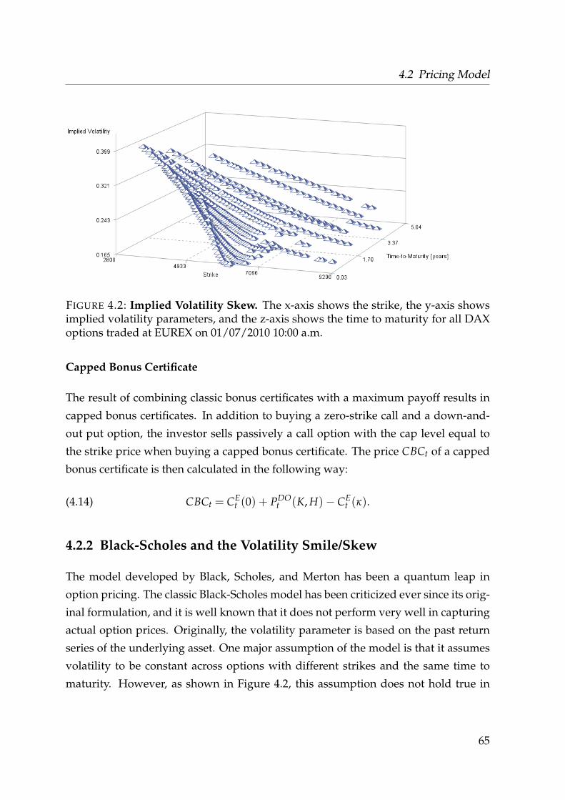
4.2 Pricing Model
FIGURE 4.2: Implied Volatility Skew. The x-axis shows the strike, the y-axis showsimplied volatility parameters, and the z-axis shows the time to maturity for all DAXoptions traded at EUREX on 01/07/2010 10:00 a.m.
Capped Bonus Certificate
The result of combining classic bonus certificates with a maximum payoff results in
capped bonus certificates. In addition to buying a zero-strike call and a down-and-
out put option, the investor sells passively a call option with the cap level equal to
the strike price when buying a capped bonus certificate. The price CBCt of a capped
bonus certificate is then calculated in the following way:
CBCt = CEt (0) + PDO
t (K, H)− CEt (κ).(4.14)
4.2.2 Black-Scholes and the Volatility Smile/Skew
The model developed by Black, Scholes, and Merton has been a quantum leap in
option pricing. The classic Black-Scholes model has been criticized ever since its orig-
inal formulation, and it is well known that it does not perform very well in capturing
actual option prices. Originally, the volatility parameter is based on the past return
series of the underlying asset. One major assumption of the model is that it assumes
volatility to be constant across options with different strikes and the same time to
maturity. However, as shown in Figure 4.2, this assumption does not hold true in
65

Chapter 4 Data and Methodology
practice. Figure 4.2 visualizes a snapshot for implied volatility parameters for DAX
options with different strikes and time to maturities on January 7, 2010 at 10:00 a.m.
Implied volatilities are higher for options with lower strikes. For a fixed time to matu-
rity, this pattern is known as volatility smile or skew due to its U-shape and it is a dis-
tinctive feature for index and equity options. The smile/skew is more pronounced for
options with shorter time-to-maturity. This pattern has first been observed after the
stock market crash in 1987, which leads to the common assumption that the volatility
smile/skew is the result of the fear of another crash in the future ("crash-o-phobia")
(cf. Rubinstein, 1994). Other explanations for the smile are influences of liquidity
and transaction costs (Peña et al., 1999). Basically, the observed volatility smile/skew
implies that out-of-the-money puts are priced considerably higher than out-of-the-
money calls. To overcome this drawback in the Black-Scholes model, I assume the
volatility parameter to be a non-constant function of time to maturity and strike. This
modification of the original model is referred to as Practitioners Black-Scholes.17 The
volatility parameter used as input parameter in the PBS model is therefore implic-
itly calculated from existing options through solving the Black-Scholes formula for σ.
Hence, I rather must have set σ = σ(K, T) in the above formulas for the calculation of
different product prices.
Due to institutional conventions, a limited number of strikes and expiry dates are
traded. Hence, implied volatility can only be derived pointwise. Even though im-
plied volatility observations are gathered in this pointwise design, practitioners think
of them as stemming from a smooth and well-behaved surface. This requires suit-
ably chosen intrapolation and extrapolation techniques or a fully specified model for
the implied volatility surface. Figure 4.3 shows a possible volatility surface for the
afore visualized option data snapshot. The following subsection outlines the implied
volatility estimation method used in this thesis.
4.2.3 Implied Volatility Estimation
I adjust the implied volatility parameter for each observation for each product in-
dependently. To estimate the volatility parameter of the underlying asset, I extract
17Very similar versions of the model are known as ad-hoc Black-Scholes model (Berkowitz, 2010) orImplied Volatility Function model (Hull and Suo, 2002).
66

4.2 Pricing Model
FIGURE 4.3: Implied Volatility Surface. The x-axis shows the strike, the y-axis showsimplied volatility parameter, and the z-axis shows the time to maturity for all DAXoptions traded at EUREX on 01/07/2010 10:00 a.m.
the implied volatility from options traded at EUREX based on time to maturity and
strike by inverting the standard Black-Scholes formula for calls and puts, respectively.
I obtain all call and put options traded at EUREX for all relevant underlying assets
within individual sample periods from SIRCA and compute the individual implied
volatility. Figure 4.4 shows the daily average implied volatility of EUREX options
with the DAX index as underlying throughout 2010. The implied volatility increased
substantially in May 2010 compared to the beginning of the year. One explanation
could be the flash crash on May 6, 2010 when the Dow Jones index lost and regained
approximately 1000 points within a few minutes.18
Instead of using an averaging procedure, the PBS model incorporates volatility
as a function of time to maturity and strike. Dumas et al. (1998) investigate several
parameterizations and find all of them to outperform a constant volatility factor. I
use the volatility function
σ(K, T∗) = α + β1K + β2K2 + ε,(4.15)
18For more information on the flash crash see, for example, Kirilenko et al. (2011).
67

Chapter 4 Data and Methodology
FIGURE 4.4: Implied Volatility Over Time. The x-axis shows the date, whereas they-axis shows the daily average implied volatility across all DAX options traded atEUREX.
where T∗ indicates the maturity of the EUREX option chains used to estimate the pa-
rameters by Ordinary Least Squares. Exact matches of the time to maturity of struc-
tured products, more precisely the incorporated (barrier) options, with options traded
at EUREX are rather rare. Accordingly, for those options where I do not have an ac-
tual fit, I use those two option chains having the closest maturity dates, from above
and below respectively, compared to the maturity date of the structured product. An
option chain denotes a collection of put and call options on the relevant underlying
beyond a wide range of strike prices but with same maturity19. As a result, I obtain
for the strike of the structured product two volatility parameter through (4.15) for the
different option chains.20 Finally, to determine the implied volatility estimate for each
observation with respect to the time to maturity, I weight both volatility estimates ac-
cording to the difference in time between maturity dates of the option chains and the
structured product. Applying the relevant volatility parameter21 for the individual
formula eventually results in the ’fair’ theoretical price of the analyzed product.
19cf. EUREX website for details, www.eurexchange.com/.20I note that in case of barrier options it is theoretically debatable whether to apply the strike level, the
barrier level, or anything in between into the implied volatility function. I test strike level, barrierlevel, as well as the average of both and find that the barrier level returns the best results in termsof standard and maximum deviation from observed prices.
21Additionally, I calculate prices using historical moving-average volatilities with horizons of up to100 days instead of the implied volatility interpolation procedure. I obtain price differences similarto those reported.
68

4.2 Pricing Model
FIGURE 4.5: Euro Interbank Offered Rate Over Time. The x-axis shows the date,whereas the y-axis shows the daily last EURIBOR distinguished by periods of 1 to 3weeks and 1 to 12 months.
For the valuation of bonus certificates in Chapter 5 the implied volatility calcula-
tions are realized on a 5 min basis. Prices for discount certificates and capped bonus
certificates are based on EOD option data.
For the risk free interest rate, I use Euro Interbank Offered Rate (EURIBOR) for
periods of 1 to 3 weeks and 1 to 12 months, and 2 year and 3 year yields of the REXP
Bond index.22 Figure 4.5 shows the EURIBOR from May 2008 until January 2011. In
2010, the sample period for later analyses, the EURIBOR has considerably decreased
compared to years before. For maturity dates that do not correspond to the exact pe-
riods of EURIBOR and REXP rates, I interpolate between the closest two rates avail-
able. For example, the desired interest rate for a period of 1,5 weeks is computed by
equally weighting the one and two week EURIBOR rate.
22ISIN DE0008469115. REXP Bond Yields are the yields of a synthetic bond containing 30 Germangovernment bonds and are reported on a daily basis by Deutsche Boerse.
69

Chapter 4 Data and Methodology
4.2.4 Limitations
I believe that the PBS model approach serves best for my analysis. Dumas et al. (1998)
investigate the model error of several different deterministic volatility functions in the
Black-Scholes model compared to observed prices for S&P 500 index options. All pro-
posed volatility functions provide better results in terms of mean squared valuation
errors than the original Black-Scholes model assuming constant volatility. Hull (2005)
and Christoffersen and Jacobs (2004) confirm these findings for European and com-
pound options and show that for this class of options the PBS model provides better
results — again with respect to the mean squared errors of model and observed op-
tion prices — than a stochastic volatility approach like the Heston (1993) model. I
assume that my implied volatility estimation performs even better due to a larger op-
tion data set than in those cited studies. Singh et al. (2011) support the effectiveness
of the PBS model compared to the standard Black-Scholes model and the Heston and
Nandi (2000) GARCH model. In case of exotic options, particularly path-dependent
options, the PBS approach has some disadvantages compared to structural stochastic
volatility models but still improves the standard Black-Scholes model (cf. Hull, 2005).
Indeed, Christoffersen and Jacobs (2004) state that PBS is by no means superior to
structural models but is useful as a benchmark. However, An and Suo (2009) exam-
ine the accuracy of hedging strategies for exotic options based on several models:
PBS, constant elasticity of variance model, stochastic volatility model, and the jump
diffusion model. All models are recalibrated whenever they are used to study them
in a practitioners-like way. They find that the PBS model performs better than alter-
native models for barrier options as long as it is frequently recalibrated. However, the
performance is strongly depending on the degree of path dependency as also pointed
out by Hull and Suo (2002).
The purpose of my analyses in this thesis is not to improve option pricing the-
ory, but in getting an intuition about the systematical (average) premium behavior of
structured products. Hence, the PBS approach seems to be the best choice to achieve
a reliable market estimation of fair prices. For a comprehensive discussion of the PBS
approach see Berkowitz (2010).
From a practitioners point of view, I emphasize the performance aspect of a pricing
model. It has to be considered that investment banks have to provide binding quotes
70

4.3 Summary
and liquidity in real time23 for up to 100,000 different structured products, something
that cannot be accomplished with sophisticated complex mathematical approaches,
such as jump diffusion models. Therefore it is more likely that issuing banks em-
ploy quick to calculate formulas or heuristics to provide continuous quotes and use
sophisticated structural models to control hedging and risk of their product portfo-
lio.24
Summarizing, I am aware that there is a potential model (selection) risk for my
analyses, but from the above argumentation, robustness checks, and related empirical
studies (e.g. Baule and Tallau, 2011) I conclude that the overall influence on the aver-
age (overpricing) premiums is negligible. I also remark that my analyses treat each
product isolated, i.e. independent of a bank’s other issued products. Consequently, I
do not account for possible synergistic effects of a large product portfolio.
4.3 Summary
In this section, I described data sources and methodological approaches that are used
in this thesis. I use quote, trade, and news data from three distinct sources to run
in-depth analyses on the market of structured products. Data from Stuttgart Stock
Exchange makes my analyses a valuable addition to the common literature, since
this data set represents the majority of exchange-traded transactions in structured
products and thus allows me to sketch a representative picture across brokers for the
entire retail investor population.25
In order to derive theoretical prices for different product types I rely on the Practi-
tioners Black-Scholes model, a variation of the standard Black-Scholes model includ-
ing a more sophisticated (implied) volatility parameter. By the use of this adapted
model I try to overcome some of the drawbacks of the classic model. In the follow-
ing chapter, I use the discussed method and data to analyze the pricing of structured
products by issuers.
23Issuers usually provide quotes several times per second depending on the current market situation.24For example, see Haug and Taleb (2011) for details about the use of heuristics by option traders.25See http://www.derivateverband.de/DEU/Statistiken/Boersenumsaetze (accessed
10/08/2013) for detailed statistics regarding stock exchange turnover for structured products inGermany.
71

Chapter 4 Data and Methodology
72

Chapter 5
Investment Banks’ Price-Setting
Behavior
”Pricing is actually a pretty simple and straight forward thing. Customers will not pay
literally a penny more than the true value of the product.”
Ron Johnson (Former Vice President at Apple Inc.)
5.1 Introduction
FFINANCIAL institutions sell products to retail investors that mimic payoffs of
complex investment strategies. The universe of such investment products is in-
creasing constantly; in 2013 more than one million structured products were tradable
in Germany.1 This market is unique in the sense that issuing banks act as the main liq-
uidity supplier and investors’ primary trading counterpart. I study the intraday and
interday pricing policy of issuers for structured investment products. I decompose
quoted product prices into two general parts: (1) the theoretical fair value; and (2) the
product premium. I analyze two different factors behind changes in premium: hedg-
ing costs and anticipation of investor demand. Investment banks hedge themselves
1See Section 2.3 for descriptive statistics on the German and other European markets.
73

Chapter 5 Investment Banks’ Price-Setting Behavior
continuously throughout the day, suggesting that hedging costs and premiums are
highly correlated. In addition investment banks may anticipate the demand for their
products and adjust prices to capture rents.
I focus on bonus certificates as one major group of traded structured investment
products2. Bonus certificates are derivatives, which provide investors with a complex
payoff structure at maturity, which is designed to reduce the risk compared to a direct
investment in the underlying instrument. Investors receive a minimum payment in
the amount of the bonus level if the underlying never touched a predefined barrier.
Due to the apparent safety of bonus certificates, bank advisers frequently offer
these products to their customers despite the hardly understandable price develop-
ment, and nontransparent inner costs. From a legal perspective, bonus certificates
are designed as bearer bonds, which permits only the issuing bank as counter party
at date of maturity, adding a default risk for the investor. During maturity, the issuing
bank acts as the major liquidity supplier allowing only limited price competition.
A bonus certificate is a synthetic product, whose constituent parts can not be
traded at common derivative exchanges, which prohibits intuitive price comparison
for retail investors. It consists of a zero-strike call and a down-and-out put barrier op-
tion. The latter increases the price-setting complexity through its path dependency.
I obtain theoretical prices using an adopted version of the Black and Scholes (1973)
modeling approach.3 I measure effects of both, intraday and interday, shifting premi-
ums on the wealth of retail investors, which is defined on a loss per trade basis.
Structured products have been subject of several studies for the last years. Gener-
ally, studies have focused on the overpricing (including a premium) of products on
a daily basis and the life cycle effect, which denotes the decrease of overpricing with
shorter maturity. For a comprehensive overview of this literature refer to Section
3.1.
This thesis contributes to the literature by providing evidence for the price-setting
behavior of investment banks for one of the most important product types for Ger-
man retail investors. Analyzing the intraday as well as the interday pricing of issuers
2Bonus certificates made up for ca. 13% of order book volume in June 2012 at German derivativeexchanges (Source: DDV).
3See Section 4.2 for more details on the pricing model.
74

5.2 Research Questions
makes it a valuable addition to existing literature. Due to a unique data set provided
by the Stuttgart Stock Exchange and continuous intraday quotes of issuers I am able
to measure precisely the effect of order anticipation of investment banks. My sample
includes all trades at Stuttgart Stock Exchange and provides an ideal basis to measure
resulting effects of the price-setting behavior on the wealth of retail investors.4
I find that investment banks quote prices above theoretical fair prices and increase
their premiums towards the end of the day. Furthermore, I find support for the life
cycle hypothesis for bonus certificates. I find that investment banks increase premi-
ums in times of high uncertainty. Additionally, investment banks react to the demand
of their products by reducing or increasing premiums depending on the type of trade.
They reduce premiums after a sell order, and they increase them after a buy order. I
provide evidence that retail investors are affected by intraday and interday shifts in
premium and that they lose approximately 1% on average of their invested capital
due to those shifts.
In extension to those results, I examine briefly premiums of products that are less
and more complex compared to bonus certificates. I find substantially lower premi-
ums for less complex products (discount certificates), and higher premiums for more
complex products (capped bonus certificates). Additionally, I analyze the compara-
bility of structured products across issuers. I find that less than 1% of all products
have an identical substitute from another issuer and thus allow for a direct price
comparison.
The remainder of this chapter is organized as follows: Section 5.2 derives research
questions addressed in this chapter. I describe my sample in Section 5.3. I identify
and analyze possible premium influences in Section 5.4 and Section 5.5 concludes.
5.2 Research Questions
This chapter addresses in particular Research Question 1, as mentioned below.
Research Question 1. Do issuers exploit the ignorance of retail investors?
4See Section 4.1 for more details on the data.
75

Chapter 5 Investment Banks’ Price-Setting Behavior
In order to identify a potential exploitation, I break this question down into several
sub questions focusing on this scenario from different perspectives. Generally, ob-
served higher prices for products relative to their theoretical values result in a greater
financial leeway for issuers, since they have more money at hand than they actually
need to build the product. Therefore, as a first step, I study the discrepancies between
quoted and theoretical prices:
Research Question 1a. What is the average premium issuers include in their
products?
Most structured products have a fixed time to maturity. Depending on the product
type it varies between a few months and several years. Assuming that more buy
than sell orders exist in the first period of a product’s life time and vice versa towards
the end, a continuous decrease of the premium until maturity resembles the gain of
almost risk-free profits for issuers. Research Question 1b captures this scenario:
Research Question 1b. How do premiums change over the life time of struc-
tured products?
In addition to the analysis of this overall time influence on the premium of structured
products, I also examine whether premiums change during the day. Regardless of a
continuous decrease of premiums over the life time, issuers might use similar patterns
during the day to anticipate investor behavior.
Research Question 1c. How do premiums change during the day?
Fortunately, I have retail trading data at my disposal, which allows me to deepen the
previous analyses by examining the direct effects of executed orders on the premium.
The following research question addresses the consideration that issuers change their
premiums depending on the current net volume.
Research Question 1d. Are issuers anticipating retail investor demand?
Additionally, I study whether changes in premium have any effect on retail investor
wealth. More precisely, I do not study the effect of market timing but the change of
premiums between buy and sell decisions of investors. This objective is reflected in
the following research question.
Research Question 1e. What is the impact of premium changes on wealth of
investors?
76

5.3 Sample Selection and Descriptive Statistics
Finally, I examine whether premiums and competition differ between overall product
types of different complexity, i.e. products that incorporate a more or less complex
option structure.
Research Question 1f. What is the effect of complexity on premiums and com-
petition of issuers?
The following section gives insights into my sample, which is used to answer the
research questions above.
5.3 Sample Selection and Descriptive Statistics
I analyze the price-setting behavior of investment banks for one of the most impor-
tant retail investor product types: (classic) bonus certificates. As underlying I focus
on the German performance index DAX. My sample consists of all trading days be-
tween January 4th, 2010 and December 31st, 2010, which results in 255 days. I obtain
intraday quote data on a 5 min basis for bonus certificates tradable at Stuttgart Stock
Exchange as well as for the DAX and XDAX from Thomson Reuters DataScope Tick
History archive through SIRCA. The XDAX is an indicator for the DAX index out-
side regular trading hours of the DAX. It is based on DAX futures traded at Eurex.
Analogously, I obtain Eurex option data (so-called option chains) for all strikes and
maturities, which are used to calibrate my pricing model, i.e. my implied volatility
parameter. On average, there are about 760 different options available on each day
during my sample period. I obtain full master data and customer trade data for all
structured investment products from Stuttgart Stock Exchange.5 I only take products
into account which have at least a trading volume, which adds up to EUR 10,000 over
their life time.
Table 5.1 reports descriptive statistics for my trade data set. I remove all bonus
certificates for which no intraday data can be obtained through SIRCA. My sample
comprises of 4,161 trades, consisting of 4,161 buy orders and 2,776 sell orders, with
a total volume of approximately EUR 250 million. The average trade size is EUR
60,302. However, the median trade size (EUR 13,479) is substantially smaller. Figure
5Refer to Section 4.1 for more information on the different data sets. A detailed description of allavailable fields of the Stuttgart Stock Exchange data is presented in Appendix D.
77

Chapter 5 Investment Banks’ Price-Setting Behavior
TABLE 5.1: Descriptive Statistics - Trades. This table captures descriptive statisticsfor the trade data sample obtained from Stuttgart Stock Exchange. It consists of 255trading days between January 4th, 2010 and December 31st, 2010.
Total
Total Volume [EUR] 250,918,523
Trade Count 4,161Number of Buys 2,776Number of Sells 1,385
Average Trade Size [EUR] 60,302.46Trade Size Std. Dev. (243,014)Median Trade Size [EUR] 13,479.01
FIGURE 5.1: Number of Trades Throughout 2010. This figure visualizes the numberof trades per month for the sample period.
5.1 shows the number of trades per month throughout the sample period. The num-
ber of trades increased considerably towards the end of the year. This effect could
be driven by tax considerations of investors (see, e.g., Barber and Odean, 2004; Grin-
blatt and Keloharju, 2004). To avoid potentially higher flat rate withholding taxes,
investors might realize losses towards the end of the year.6
I exclude all observations of bonus certificates later than 2 p.m. on December, 30th
due to the final reporting of the DAX in 2010. I report descriptive statistics for my
quote data sample in Table 5.2. My sample includes 930 products issued by six dif-
6In Germany, the flat rate withholding tax came effective on January, 1st 2009.
78

5.3 Sample Selection and Descriptive Statistics
TABLE 5.2: Descriptive Statistics - Quotes. My sample consists of 930 structuredproducts tradable in 2010 issued by six different investment banks (A to F). This tablereports the mean maturity (T∗− t0)/365 (where t0 is the issuance date) in years, mon-eyness (St0 −K)/K (where K is the strike price and St0 the DAX level at issuance) andmean cushion to barrier H (St0 − H)/H at products’ issuance. Standard deviationsare reported in parantheses.
Investment Bank #Products Maturity Moneyness Cushion
A 322 0.98 -0.27 0.28(0.62) (0.10) (0.17)
B 63 1.05 -0.09 0.24(0.43) (0.04) (0.11)
C 77 0.85 -0.18 0.31(0.34) (0.11) (0.15)
D 85 1.30 -0.29 0.25(1.15) (0.09) (0.27)
E 100 0.56 -0.36 0.17(0.28) (0.06) (0.08)
F 283 0.98 -0.37 0.33(0.53) (0.09) (0.21)
Total 930 0.96 -0.29 0.28(0.63) (0.12) (0.19)
79

Chapter 5 Investment Banks’ Price-Setting Behavior
FIGURE 5.2: Moneyness and Maturity Across Products. This figure visualizes theaverage moneyness and maturity across all products and issuers for the entire sampleperiod.
ferent investment banks, which results in 12,631,403 quotes. Products in my sample
have an average time to maturity of 0.96 years and an average moneyness of -29%,
which is the difference between underlying price and bonus level divided by bonus
level. The average relative difference to the barrier (cushion) is 28%. However, these
characteristics differ between investment banks. Due to data protection policies of the
Stuttgart Stock Exchange, I make investment banks anonymous by relabeling them
alphabetically. Average time to maturity ranges from 0.56 years for investment prod-
ucts of bank F to 1.30 years for bank D products, whereas moneyness ranges from
-37% (bank F) to -9% (bank B). Figure 5.2 visualizes average maturity and moneyness
across all products and observations throughout the sample period. As shown in Fig-
ure 5.3 the average moneyness across products does not vary substantially between
months. However, the range of moneyness values increases towards the end of the
year. Values for the cushion range from 17% (bank E) to 33% (bank F).
80

5.4 Results
FIGURE 5.3: Moneyness Across Products Over Time. The x-axis shows the monthsof the year 2010, whereas the y-axis shows the average moneyness across productsvisualized as a box plot.
5.4 Results
This section presents results for all previously mentioned research questions in this
chapter.
5.4.1 Premiums of Investment Banks
This section aims to provide an answer to Research Question 1a:
Research Question 1a. What is the average premium issuers include in their
products?
To measure the effect of overpricing for structured investment products, I define the
absolute premium Pabsit of a product i at time t (5 min intervals) as the difference
between the observed quoted price BCobsit and the calculated theoretical price BCthe
it :
Pabsit = BCobs
it − BCtheit .(5.1)
81

Chapter 5 Investment Banks’ Price-Setting Behavior
The relative premium is defined as
Prelit =
Pabsit
BCobsit
100.(5.2)
Refer to Section 4.2.1 for more information on the calculation of theoretical prices for
bonus certificates. Since issuers do not offer free lunch and short selling is not possible
in such products, I expect premiums to be positive, i.e. Pabsit , Prel
it ≥ 0. Achieving
arbitrage profits based on high premiums is nearly impossible for retail investors due
to restricted market access, high transaction costs, and the inability to go short.
The following subsections analyze different effects and characteristics of overpric-
ing and its impact on retail investor wealth. I report overall relative premiums in
Table 5.3 clustered by issuing investment bank, since there are distinct differences
between them. In total, premiums for all issuers are 2.80% across all products and
days. Premiums range from -0.39% (bank B) to 4.09% (bank F). Reported results are
TABLE 5.3: Average Issuer Premiums and Spreads - Bonus Certificates. This tablereports average spreads, and relative price deviations in percent between calculatedtheoretical prices and observed quotes.
Investment Bank Premium [%] Std. Dev. Spread [EUR] Spread [%]
A 2.20 3.54 0.04 0.03B -0.39 1.42 0.06 0.05C 1.10 2.41 0.05 0.03D 3.74 3.43 0.08 0.05E 3.85 2.60 0.06 0.04F 4.09 4.08 0.13 0.08
Total 2.80 3.74 0.07 0.05
similar to Entrop et al. (2011), although my sample has an average time to maturity
of 0.97 years for which they obtain a considerably higher value of 1.74 years, which
drives to some extent premiums as will be discussed later on. Premiums for bonus
certificates are higher than for less complex products such as discount certificates,
for which Baule (2011) finds that premiums are roughly 0.42% across all investment
banks. Figure 5.4 visualizes average monthly premiums across products throughout
the sample period. The monthly standard deviation of premiums - with the excep-
82

5.4 Results
FIGURE 5.4: Premium Across Products Over Time. The x-axis shows the months ofthe year 2010, whereas the y-axis shows the average monthly premium across prod-ucts visualized as a box plot.
tion of June - is roughly similar over the sample period. In June, however, standard
deviations are considerably larger. Note that calculated premiums are conservative,
since I do not include the default risk of the issuer in my methodological approach.
Controlling for the default risk premiums should be slightly higher.
5.4.2 Intraday and Interday Effects
The pricing policy of issuers is unknown to investors. Neither do they provide suffi-
cient information about their theoretical modeling approach, nor do they say some-
thing about their algorithms accuracy relative to their chosen model. In the following
sections, I provide some empirical insights on the price-setting behavior of issuers
and whether they take advantage of their strategic position and the ignorance about
price modeling of retail investors. To begin with, I focus on timing influences as facil-
itated in Research Question 1b and 1c:
Research Question 1b. How do premiums change over the life time of struc-
tured products?
Research Question 1c. How do premiums change during the day?
83

Chapter 5 Investment Banks’ Price-Setting Behavior
Existing studies (see Section 3.1) are usually using daily quoted prices, i.e. EOD data,
to detect issuer overpricing. I am focusing on the intraday price-setting behavior of
issuers and expect product premiums to be a non-invariant function of the time of
the day. I group quotes by the hour, putting the first and last 30 minutes of each
trading day in a separate group, e.g. group 10:00 contains all quotes from 09:30 a.m.
until 10:29 a.m. Since I use 5 min intervals this sums up to 12 quotes per product and
group, ignoring the first and the last group, which each only hold 6 quotes per prod-
uct. I build dummy variables Hour for each of the hour groups of the day. Let RTtM
denote the relative time to maturity (T∗ − t)/(T∗ − t0) as proxy for the interday ef-
fect. Additionally, moneyness has been found an important factor regarding issuers’
premiums (cf. Baule, 2011). Thus, let Money denote the moneyness (St − K)/K for
an observation for a product with strike K. To control for different pricing behaviors
between investment banks, I build dummy variables Bank for individual investment
banks. In order to explore the existence of both phenomena, intraday and interday
shifts, I run a regression model across all observations of all products:
Prelj = α + β RTtMj + γMoneyj +
19
∑i=9,i 6=13
δi Hourij +5
∑k=2
τk Bank jk + εj,(5.3)
where Prelj denotes the relative premium of observation j.
Prior studies show that - for some product types - issuers decrease premiums sys-
tematically during the life of an investment product, which has been called the life
cycle hypothesis (Muck, 2006). Investors tend to buy structured products in the be-
ginning of a product’s life time and tend to sell it before maturity as visualized in
Figure 5.5. I calculate the trading frequency across all products over the whole sam-
ple period with respect to the remaining time to maturity for each product. The buy
and sell frequency appears to be diametrically opposed to each other. Hence, with
a systematic decrease of premiums over time, issuers increase their rents, since, on
average, investors buy for higher prices and sell for lower prices. Thus, I expect the
coefficient of the remaining time to maturity to be positive, to measure the effect if
issuers decrease their premiums with a reduced time to maturity. As for the intra-
day effect, I expect estimates of the hour dummies to be different from each other.
The moneyness variable can assume positive and negative values, depending on the
84

5.4 Results
FIGURE 5.5: Trading Frequency With Respect to Maturity. The x-axis shows thepercentage product life time that has passed, whereas the y-axis shows the tradingfrequency across all products in my sample.
difference between current underlying price and bonus level. Figure 5.6 visualizes
the value of the incorporated barrier option of a bonus certificate with respect to the
underlying price. The down-and-out put option value becomes very small for strong
positive moneyness values, i.e. on the right side of the second dashed line in Figure
5.6. On the other hand, the barrier option value changes substantially for negative
moneyness values. The value of the barrier option is not transparent to the investor,
and thus provides the ideal environment for issuers to incorporate a higher premium
as the underlying asset approaches the barrier. Nevertheless, issuers could face an
increased hedging risk if the underlying approaches the barrier, since their valua-
tion approach might result in higher model failures and, thus, inaccurate hedging
positions. A higher premium would compensate the issuer for such increased risks.
Therefore, I expect moneyness to have a negative effect on premiums, i.e. an in-
creasing premium with decreasing moneyness, as also reported by Baule and Tallau
(2011).
Table 5.4 reports results for the regression model differentiating between three sce-
narios. First, I skip the remaining time to maturity and moneyness variable to focus
on the intraday effect. Second, I exclude all hour dummies but include moneyness
and remaining time to maturity to measure the interday effect; and third, the combi-
nation of both. I correct standard errors for heteroscedasticity effects and serial corre-
lation using the procedure proposed by Newey and West (1987). I find that premiums
change constantly throughout the day. Premiums between 3 p.m. and 4 p.m., as well
85

Chapter 5 Investment Banks’ Price-Setting Behavior
TABLE 5.4: Intraday and Interday Premium Shifts. I analyze intra- and interdaypremium shifts for bonus certificates. RTtM denotes the relative time to maturity(T∗ − t)/(T∗ − t0), Money denotes the moneyness (St − K)/K with strike K at thattime. I include dummy variables for the hour of the day and individual investmentbanks. T-values are reported in parentheses. */**/*** denotes significance on the 5%,1%, 0.1% level.
Intraday Interday Combined
Intercept 2.17*** -3.07*** -3.09***(403.06) -(498.41) -(463.10)
RTtM 1.25*** 1.25***(135.54) (135.44)
Money -21.15*** -21.15***(-851.20) (-851.27)
09:00 0.03*** 0.04***(4.84) (7.83)
10:00 0.01* 0.01**(2.09) (2.62)
11:00 0.00 0.00(0.76) (1.00)
12:00 0.00 0.00(-0.86) (-0.96)
14:00 0.01 0.00(0.27) (1.31)
15:00 0.03*** 0.02***(4.34) (6.22)
16:00 0.04*** 0.04***(7.07) (9.90)
17:00 0.01* 0.01(1.97) (1.31)
18:00 0.07*** 0.07***(12.61) (16.50)
19:00 0.09*** 0.08***(12.62) (16.88)
Bank B -2.58*** 2.37*** 2.37***(-499.93) (403.88) (403.97)
Bank C -1.10*** 0.55*** 0.55***(-135.25) (65.83) (65.85)
Bank D 1.54*** 1.27*** 1.27***(214.62) (313.49) (313.50)
Bank E 1.66*** -0.85*** -0.84***(207.15) (-133.71) (-133.50)
Bank F 1.89*** 0.13*** 0.13***(305.24) (29.22) (29.21)
Adj. R2 0.12 0.57 0.5786

5.4 Results
0
10
20
30
50 75 100 125 150Underlying Price
Opt
ion
Val
ue
FIGURE 5.6: Black-Scholes Value of a Down-and-out Put Option. The x-axis showsthe underlying price, whereas the y-axis shows Black-Scholes model values for adown-and-out put option with strike K = 100, barrier H = 50, volatility σ = 0.15,risk-free interest rate r = 0.02, time to maturity T = 1, and dividend yield q = 0.
as after 5:30 p.m., when the daily final official DAX value is reported, are higher com-
pared to the rest of the day. For example, premiums between 6:30 p.m. and 7:00 p.m.
are, on average, 0.09% higher compared to premiums at 1:00 p.m. Investment banks
include an overnight (gap) risk of the underlying into their premium (cf. Entrop et al.,
2011). The overnight risk should compensate issuers for potentially higher hedging
costs if unexpected news hit the market and price leaps occur, which could result in
an imperfect hedging situation for the issuer. Hedging costs may increase after main
trading hours due to higher spreads and lower liquidity. Hence, my intraday increase
in premium towards the end of the day might be due to the adjustment of prices to
the overnight risk. As robustness check, I also run the regression separately for is-
suers. Table 5.5 reports the results. Besides for issuer C the pattern is consistent for
all issuers.
Since investment banks are liquidity provider, wider spreads have to be seen as
additional premium. A change in premium could therefore be offset by a reduced
spread. I calculate relative and absolute spreads in basis points for all observations
and find that the hour of the day and relative spreads at Stuttgart Stock Exchange are
correlated with factor 0.00069, which is negligible. Absolute spread values change
by just one cent within days and are typically about 7 cent, which corresponds to a
0.05% relative spread (see Table 5.3). Therefore, spreads do not matter regarding the
87
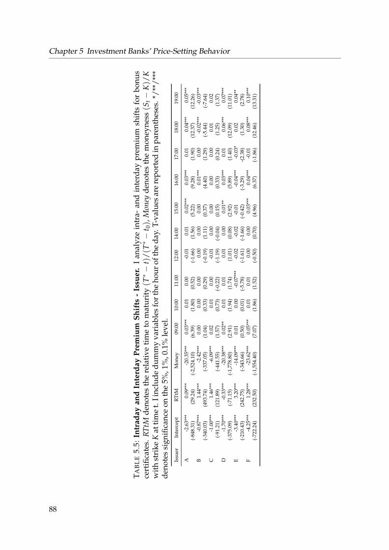
Chapter 5 Investment Banks’ Price-Setting Behavior
TAB
LE
5.5:
Intr
aday
and
Inte
rday
Prem
ium
Shif
ts-
Issu
er.
Ian
alyz
ein
tra-
and
inte
rday
prem
ium
shif
tsfo
rbo
nus
cert
ifica
tes.
RTtM
deno
tes
the
rela
tive
tim
eto
mat
urit
y(T∗−
t)/(T∗−
t 0),
Mon
eyde
note
sth
em
oney
ness
(St−
K)/
Kw
ith
stri
keK
atti
me
t.Ii
nclu
dedu
mm
yva
riab
les
fort
heho
urof
the
day.
T-va
lues
are
repo
rted
inpa
rent
hese
s.*/
**/*
**de
note
ssi
gnifi
canc
eon
the
5%,1
%,0
.1%
leve
l.Is
suer
Inte
rcep
tR
TtM
Mon
ey09
:00
10:0
011
:00
12:0
014
:00
15:0
016
:00
17:0
018
:00
19:0
0
A-2
.63*
**0.
09**
*-2
0.35
***
0.03
***
0.01
0.00
-0.0
10.
010.
02**
*0.
03**
*0.
010.
04**
*0.
05**
*(-
848.
31)
(29.
24)
(-2,
524.
10)
(6.3
9)(1
.80)
(0.5
2)(-
1.66
)(1
.56)
(5.2
2)(9
.28)
(1.9
0)(1
2.37
)(1
2.26
)B
-0.8
7***
1.44
***
-2.4
2***
0.00
0.00
0.00
0.00
0.00
0.00
0.01
***
0.00
-0.0
2***
-0.0
3***
(-34
0.03
)(4
93.7
4)(-
337.
05)
(1.0
4)(0
.33)
(0.2
9)(-
0.19
)(1
.11)
(0.3
7)(4
.40)
(1.2
9)(-
5.44
)(-
7.64
)C
-1.0
0***
1.46
***
-6.0
9***
0.02
0.01
0.00
-0.0
10.
000.
000.
000.
000.
010.
02(-
91.2
1)(1
21.8
9)(-
441.
55)
(1.5
7)(0
.73)
(-0.
22)
(-1.
19)
(-0.
04)
(0.1
5)(0
.33)
(0.2
4)(1
.25)
(1.3
7)D
-1.7
0***
-0.3
3***
-20.
38**
*0.
02**
0.01
0.01
0.01
0.00
0.01
**0.
03**
*0.
010.
06**
*0.
07**
*(-
375.
09)
(-71
.15)
(-1,
778.
80)
(2.9
1)(1
.94)
(1.7
4)(1
.01)
(0.0
8)(2
.92)
(5.8
9)(1
.40)
(12.
09)
(11.
01)
E-3
.40*
**3.
20**
*-1
4.09
***
0.01
0.00
-0.0
7***
-0.0
2-0
.02
-0.0
1-0
.04*
**-0
.03*
0.02
0.04
**(-
210.
43)
(242
.75)
(-34
3.66
)(0
.50)
(0.0
1)(-
5.78
)(-
1.61
)(-
1.66
)(-
0.42
)(-
3.29
)-(
2.38
)(1
.30)
(2.7
8)F
-4.2
5***
1.28
***
-23.
62**
*0.
05**
*0.
010.
010.
000.
000.
03**
*0.
04**
*-0
.01
0.08
***
0.10
***
(-72
2.24
)(2
32.5
0)(-
1,55
4.40
)(7
.07)
(1.8
6)(1
.52)
(-0.
50)
(0.7
0)(4
.96)
(6.3
7)(-
1.86
)(1
2.46
)(1
3.31
)
88

5.4 Results
timing decision of retail investors’ trades. This does not apply for OTC platforms
after 8 p.m., for which it can be observed that spreads are pushed further apart. Since
bonus certificates are long term investment products, it usually does not matter for
investors at which time of the day their orders get executed, assuming that investors
do not have any knowledge about future price movements. Anticipation of intraday
premium shifts could therefore increase investor profits.
As for the interday effect the regression estimate for the relative time to maturity
is positive (1.25∗∗∗), which means that premiums decrease with a shorter time to ma-
turity. Put differently, investors, who bought at the issuance day and did not sell
before the last day lost, on average, 1.25% through the reduction of the incorporated
premium. The premium decrease throughout a product’s life might not be due to the
attempt to increase profits for the issuer, but by the successive amortization of issuers
original distribution allowance. Although, such an allowance usually exists only for
more exotic products and not for classic products such as bonus certificates.
Moneyness has a negative influence on premiums (-21.15∗∗∗), which means that
products closer to the barrier, i.e., where moneyness is smaller than zero, include a
higher premium than those with a higher moneyness. Dummy variables for banks
indicate that premiums for banks D, E and F are, on average, higher than premiums
of bank A, whereas premiums of bank B and C are lower on average, which can be
also seen in Table 5.3.
If the barrier has been touched the bonus payment is gone and the theoretical price
of such a product is in my case simply the value of the underlying index multiplied
with the subscription ratio because there are no dividend payments. Since the com-
plexity of the product decreased substantially and risks are highly reduced for the
issuer one might expect the premium to be non-time-dependent anymore. In fact by
running the simple regression model
Prelj = α + β RTtMj + εj(5.4)
for all observations for bonus certificates that are bonus-free I still observe a strong
significant effect of the relative remaining time to maturity (α = 0.28∗∗∗, β = 0.43∗∗∗).
Such premiums cannot be mistaken for risk compensation of issuers, but for the pur-
pose to increase profits. This fact also confirms that a part of the premium is added
89

Chapter 5 Investment Banks’ Price-Setting Behavior
at issuing date and decreases continuously until maturity regardless of the actual de-
velopment of any underlying factors.
5.4.3 Risk and Demand Effects
As shown in the former section, there are intraday as well as interday influences
on premiums. Some effects can be explained through the life cycle hypothesis or
the overnight risk. In order to evaluate, independently from timing factors, whether
market risk and investor demand have any effect on the pricing policy of investment
banks, as facilitated in the following research question, I run another regression.
Research Question 1d. Are issuers anticipating retail investor demand?
To capture market risk, I calculate a volatility measure adapted to my purpose. Let
Volaj denote the relative range of the underlying within the last five minutes before
observation j. Let pt denote the underlying price at time t (in minutes), and let t0(j)
be the time of observation j. Volaj is then calculated as follows:
Volaj =
(max
t0(j)−5≤t≤t0(j)pt − min
t0(j)−5≤t≤t0(j)pt
)(
12
(max
t0(j)−5≤t≤t0(j)pt + min
t0(j)−5≤t≤t0(j)pt
))−1
100.(5.5)
My regression model is then defined as follows:
Prelj = α + βSellj + γ Buyj + δ Volaj +
5
∑k=2
τk Bank jk + εj,(5.6)
where the Buy and Sell variable are dummies that are set to one if between the last
observation and the current observation a buy or sell order was executed, respec-
tively. All other variables are as defined before. Table 5.6 reports results for three
different variations of the regression model. First, I skip the volatility variable (De-
mand); second, I exclude the buy and sell dummies (Risk), and, third, I run the model
including all variables (Combined). I observe a positive estimate for the buy dummy
and a negative estimate for the sell dummy. Generally, this could be interpreted as a
way of influencing the attractiveness of a product, similar to a classic dealer response
90

5.4 Results
TABLE 5.6: Risk and Demand Effects. This table reports effects of risk and demandon issuers’ premiums. I run the following regression Prel
j = α + βSellj + γ Buyj +
δ Volaj + ∑5k=2 τk Bank j,k + ε , where the buy and sell variable are dummies that are set
to one if between the last observation and the current observation a buy or sell orderwas executed. Vola measures the relative range of the underlying within the last fiveminutes before each observation. All other variables are as defined before. T-valuesare reported in parentheses. */**/*** denotes significance on the 5%, 1%, 0.1% level.
Demand Risk Combined
Intercept 2.20*** 1.92*** 1.92***(1,355.46) (862.16) (862.10)
Buy 1.43*** 1.37***(21.17) (19.94)
Sell -0.69*** -0.72***(-7.18) (-7.44)
Vola 2.44*** 2.44***(194.29) (194.22)
Bank B -2.58*** -2.59*** -2.59***(-653.82) (-614.96) (-614.95)
Bank C -1.10*** -1.04*** -1.04***(-217.93) (-194.16) (-194.21)
Bank D 1.54*** 1.53*** 1.53***(497.94) (463.01) (463.06)
Bank E 1.66*** 1.72*** 1.72***(325.36) (315.82) (315.78)
Bank F 1.89*** 1.89*** 1.89***(767.19) (718.05) (718.02)
Adj. R2 0.12 0.13 0.13
91

Chapter 5 Investment Banks’ Price-Setting Behavior
FIGURE 5.7: Average Intraday Premium and Volatility. The x-axis shows the hourof the day, whereas the y-axis shows volatility and percentage premium. The blacklines denotes volatility, whereas the gray line represents relative premium.
in a hybrid market (cf. Harris, 2003). If a sell order of an investor is executed, less
shares of the product are outstanding and this way investment banks do make less
risk-free profits. By decreasing the premium after a sell order, the price of the product
is better compared to competing products and more order flow may be attracted by
it. Another explanation is that issuers are decreasing premiums when they expect
sell orders to dominate and increase them if they expect buy orders to dominate. As
a result issuers would increase their profits. Those results support Baule (2011), who
uses order flow imbalances to analyze this phenomena.
The estimate for the volatility parameter is positive (2.44∗∗∗), which makes it easy
to conclude that a higher volatility, and therefore higher potential risks and associ-
ated hedging costs for the issuing bank, increase premiums substantially. Figure 5.7
visualizes average premiums across products, and the average underlying volatility
throughout the day based on five minute intervals. I observe that the highest pre-
mium peaks are consistent with a strong increase in volatility. The peak is roughly
at 3:30 p.m., at the time when markets in the USA are opening. It seems that high
uncertainty of price movements is reflected in premiums of structured investment
products.
92

5.4 Results
FIGURE 5.8: Relative Intraday Trade Frequency. This figure visualizes the averagerelative frequency of all trades included in my sample. The x-axis shows the hourof the day, whereas the y-axis shows the percentage of executed trades within theindividual hour.
5.4.4 Premium Impact on Retail Investor Wealth
Investor wealth is reduced through premiums of investment banks. Nevertheless,
premiums are necessary to compensate banks for arising risks, hedging costs, and the
service they provide to fulfill strategies for retail investors that would not be possible
otherwise. Investment banks shift premiums during the day and over the life time
of their investment products as shown in Section 5.4.2. I study the influence of those
intraday and interday shifts in premium on retail investors wealth, as stated in the
following research question.
Research Question 1e. What is the impact of premium changes on wealth of
investors?
To answer this question, I conduct a simple method based on retail trading data from
Stuttgart Stock Exchange. Obviously, retail investors’ trade frequency is not homoge-
neous throughout the day. Figure 5.8 visualizes their intraday trading activity based
on all trades in my sample. Ignoring the peak of executed orders at 9:00 a.m., which
contains all orders that have been sent to the exchange outside trading hours, the
highest relative share of executed orders is at 4:00 p.m.. This is very likely due to the
market opening in the U.S., which usually induces increased market activity in Ger-
many. Since I already know that premiums are high at that time and after the final
93

Chapter 5 Investment Banks’ Price-Setting Behavior
FIGURE 5.9: Relative Intraday Buy and Sell Frequency. This figure visualizes theaverage relative frequency of all executed buy and sell orders included in my sample.The x-axis shows the hour of the day, whereas the y-axis shows the percentage ofexecuted buy and sell orders relative to all trades. The black line denotes buy orders,whereas the gray line represents sell orders.
daily closing price for the DAX (cf. Figure 5.7), I expect intraday premium shifts to
have an influence on investors’ wealth.
Figure 5.9 shows the intraday trade frequency separated by trade direction across
all products and throughout the whole sample period. Interestingly, referring to the
time of order execution, I do not observe a different behavior of retail investors re-
garding their decision to buy or sell bonus certificates. Graphs for the relative num-
ber of buy and sell orders move very alike. In total there are more executed buy
orders than sell orders, which is probably due to the fact that investors can hold their
products until maturity. The value of the product is cashed out automatically by the
individual broker at that date without the need to sell it.
In the following I analyze how changes in premium are reflected in the wealth of
retail investors. Hence, I measure the intraday and interday impact for all trades in
product i by calculating an imbalance based on order size and the absolute premium
of the corresponding issuer for the product at that time. Let Bi and Si denote the set
of all executed buy and sell orders in product i, respectively. Moreover, let |Bi| and
|Si| denote the number of buy and sell orders in product i, respectively. I define the
94

5.4 Results
premium impact PIi as
PIi =
∑j∈Bi
−sjPabsit0(j) + ∑
k∈Si
skPabsit0(k)
∑j∈Bi
sj pj100,(5.7)
where sl denotes the size of trade l, pl denotes the execution price of trade l, and t0(l)
denotes the timestamp of the particular trade. I round trade timestamps up to 5 min
intervals to match my quote data. My premium impact measure is only comparable
across products if, for an individual product, the same number of shares have been
bought and sold during my sample period. Hence, if the aggregated number of shares
traded in product i is not equal to zero at the end of the observation period, i.e.
∑j∈Bi
sj − ∑k∈Si
sk 6= 0,(5.8)
I assume the buy or sell, depending on a positive or negative inventory, of the residual
shares given the last observed premium. For example, if until the end of my sample
period investors sold 100 shares less than they bought of product i, I assume the sell
of 100 shares with respect to last observed premium for product i. This way, I always
receive an outstanding number of zero shares and thus make the premium impact
comparable across products. If the measure above is significantly different from zero,
investors are affected by intraday and interday premium changes. Note that investors
would benefit from changes in premium if PI > 0 on average.
To further study the premium effect, I break down the premium impact measure
into intraday and interday effects. However, it has to be mentioned that this is not
possible in a exact way, thus the addition of outcomes of the intraday and interday
measures is not the same as the overall premium impact measure. Nevertheless, the
intraday and interday measure try to capture the effects as good as possible.
Assume the same setting as above. Let PabsiD(l) denote the mean absolute premium
of product i at the day when trade l was executed. I model the intraday premium
95

Chapter 5 Investment Banks’ Price-Setting Behavior
impact as follows:
PIIntraiD =
∑j∈Bi
−sj
(Pabs
it0(j) − PabsiD(j)
)+ ∑
k∈Si
sk
(Pabs
it0(k)− Pabs
iD(k)
)∑
j∈Bi
sj pj100.(5.9)
Basically, I sum up the differences between premiums at individual trade timestamps
and the corresponding daily mean of premiums with respect to the invested volume.
To measure explicitly the interday effect, I ignore premium fluctuations during the
day and, thus, use the original premium impact measure with daily average premi-
ums instead of premiums at the exact trade timestamp:
PIInteri =
∑j∈Bi
−sjPabsiD(j) + ∑
j∈Si
sjPabsiD(k)
∑j∈Bi
sj pj100.(5.10)
I expect the interday effect to be far greater than the intraday effect, since it is the
ideal way to anticipate retail investor trading behavior. The reduction of the premium
over time and, thus, the slightly reduction of potential returns has to be accepted by
investors, provided that they choose bonus certificates as their desired investment
opportunity. To gain profits following their long term investment strategy they have
to tolerate that investment banks will take their share of those profits. However, this
passive way of reducing investors profits is hard to detect for the common investor.
Results for all three measures are reported in Table 5.7.
For the first measure, the combination of both premium effects, I observe estimates
from -1.37% (bank F) to −0.40% (bank D), at which all estimates but for bank D are
significant. On average, retail investors lose roughly 1% of their invested capital due
to shifts in premium. It seems likely that investment banks are using shifts in pre-
mium to obtain additional benefits at the expense of retail investors.
By breaking up those effects into intraday and interday shifts, I observe that in-
traday losses range from 0.23% for bank A to 0.00% for bank E. Interday effects are
substantially larger than intraday effects as expected. Losses range from 1.19% (bank
F) to 0.20% (bank D). Summarizing, bad timing reduces investor wealth by 0.17%
on average, but holding products over long periods substantially reduces wealth by
96

5.4 Results
TAB
LE
5.7:
Impa
cton
Ret
ail
Inve
stor
sW
ealt
h.Th
ista
ble
repo
rts
reta
ilin
vest
ors
loss
esdu
eto
intr
aday
and
inte
rday
prem
ium
chan
ges.
Res
ults
are
repo
rted
into
tal
and
for
each
inve
stm
ent
bank
sepa
rate
ly.
T-va
lues
are
repo
rted
inpa
rent
hese
s.*/
**/*
**de
note
ssi
gnifi
canc
eon
the
5%,1
%,0
.1%
leve
l.
All
AB
CD
EF
Com
bine
dA
vera
gePr
emiu
mSh
iftL
osse
s[%
]-0
.97*
**-1
.03*
**-0
.42*
**-0
.72*
**-0
.40
-0.5
6***
-1.3
7***
T-V
alue
(-5.
02)
(-3.
76)
(-2.
82)
(-4.
44)
(-0.
58)
(-4.
87)
(-2.
89)
Intr
aday
Ave
rage
Prem
ium
Shif
tLos
ses
[%]
-0.1
7*-0
.23
-0.0
4-0
.01
-0.2
00.
00-0
.19
T-V
alue
(-1.
92)
(-1.
08)
(-1.
18)
(-0.
56)
(-1.
48)
(-0.
08)
(-1.
74)
Inte
rday
Ave
rage
Prem
ium
Shif
tLos
ses
[%]
-0.8
0***
-0.8
1***
-0.3
8**
-0.7
4**
-0.2
0-0
.56*
***
-1.1
9**
T-St
at(-
4.23
)(-
4.76
)(-
2.49
)(-
4.72
)(-
0.25
)(-
4.87
)(-
2.29
)
97

Chapter 5 Investment Banks’ Price-Setting Behavior
0.80%.
In the following I extend the prior analysis by focusing briefly on the effect of
complexity on the pricing behavior of issuers. Besides already mentioned influencing
factors, the complexity of the environment or the product might have an influence on
issuers’ premiums.
5.4.5 Complexity Effect
The success of these products and competition between the issuing banks appears to
be leading issuers to introduce more and more complex products. The payoff profiles
are becoming so complex that, at least, the average investor is unable to price them.
The increase in the number of possible products is making the comparison of similar
products across issuers onerous. Nonetheless, investors appetite for these products
appears to be unsated, perhaps to the detriment of their investment goals. This sec-
tion aims to provide a brief overview of the complexity effect on the premiums and
competition of issuers as facilitated in the following research question.
Research Question 1f. What is the effect of complexity on premiums and com-
petition of issuers?
Related Work. The study of the impact of complexity on investors’ welfare and
decision making is relatively new. Brunnermeier and Oehmke (2009) provide an
overview of complexity in financial markets and address a number of questions about
the regulation, definition, and ways to deal with complexity. Carlin (2009) develops
a model that studies complexity in retail financial markets under competition. Elli-
son and Wolitzky (2012) develop a model in which firms engage in obfuscation when
selling a homogeneous good to consumers who incur search costs. They show that
as long as obfuscation, which is positively correlated with search costs, is costless,
obfuscation must occur in equilibrium. Carlin and Manso (2010) show that educa-
tional programs designed to increase investor sophistication may actually increase
the complexity in a market.
Little empirical evidence exists on the direct impact of complexity on investor wel-
fare, investor behavior, or portfolio decisions. One exception is the experimental
98

5.4 Results
study presented in Carlin et al. (2013). They show that increased complexity leads
to lower liquidity, higher volatility, and less price efficiency. The experiment gener-
ally confirms the conjecture that investors do not deal well with complex decisions.
Arora et al. (2011) show, even in markets with fully rational investors, that asymmet-
rically distributed computational resources required to price certain derivatives can
cause market imperfections associated with asymmetric information.
Methodology and Results. Adding complexity to the structure of a product makes
the calculation of the true price more costly, i.e. the more components a product has
the harder it is for investors to derive fair prices. In the following, I study briefly
two additional product types, discount certificates and capped bonus certificates, to
measure the influence of additional components in the product structure on issuer
premiums. Both product types are related to classic bonus certificates. Discount cer-
tificates are easier to understand and less complex due to missing barrier options,
whereas capped bonus certificates add a component to bonus certificates through the
additional capped payoff. Refer to Section 4.2.1 for more information on the individ-
ual product structure. I calculate theoretical prices for both product types analogous
to the former sections. However, I base calculations on EOD data for the year 2010 for
all products having a DAX constituent or the DAX itself as underlying. Therefore, I
retrieve additional EUREX option data on a daily basis for all DAX constituents from
SIRCA. In total, I analyze 9,550 discount certificates and 4,684 capped bonus certifi-
cates issued by the same investment banks as before. Table 5.8 reports premiums for
both product types across all products and distinguished by issuer.
Premiums for discount certificates are very low on average, ranging between
0.10% (bank D) and 0.53% (bank A), compared to bonus certificates. Discount cer-
tificates are the most popular product type in Germany. Due to the more comprehen-
sible structure and the huge competition across issuers premiums might be pushed
to the lowest extent possible. However, premiums for capped bonus certificates are
substantially higher, ranging between 3.71% (bank A) and 4.57% (bank F) across all
products, which can be seen in favor of the assumption that higher complexity leads
to obfuscation and therefore allows for higher premiums. Nevertheless, from an out-
side perspective it is not possible to assess to which extent a more complex product
structure increases costs on the issuer side.
99

Chapter 5 Investment Banks’ Price-Setting Behavior
TABLE 5.8: Average Issuer Premiums - Discount and Capped Bonus Certificates.This table reports average relative price deviations in percent between calculated the-oretical prices and observed quotes for discount certificates and capped bonus certifi-cates.
Discount Certificates Capped Bonus CertificatesInvestment Bank # Premium [%] Std. Dev # Premium [%] Std. Dev
A 1,730 0.53 1.56 1,172 3.71 4.57B 3,662 0.38 1.75 946 3.95 4.69C 3,168 0.52 1.55 1,296 4.34 5.22D 830 0.10 1.34 129 4.28 4.29E 0 n/a n/a 265 4.43 5.84F 160 0.46 1.03 876 4.57 5.12
Total 9,550 0.43 1.61 4,684 4.13 4.92
Similarly, by increasing the number of similar but not exactly comparable products
issuers increase the search costs for investors such that they are unable to learn the
true (market) price from the prices of other products. In the following I study prod-
ucts tradable at Stuttgart Stock Exchange between January 1, 2009 and December 31,
2011. More precisely, I focus on discount certificates, bonus certificates, and capped
bonus certificates. For each product I analyze whether products with the exact same
or slightly similar characteristics are available. In the following, I call those products
substitutes. Figure 5.10 visualizes the workflow of the algorithm to find substitutes.
The algorithm passes step-by-step through all products and searches for each indi-
vidual product all available substitutes based on the specific configuration. If it finds
at least one substitute the result is 1 else 0.
I use four different configurations to find substitutes. All of them assume that
available substitutes should be of the same overall option type (call or put) and des-
ignated on the same underlying asset. Other characteristics, the algorithm is based on
to find substitutes, are: first trading day, last trading day, barrier level, bonus level,
and cap level. Those are varied between configurations (model A to D). Model A
defines a substitute as a product that is identical to the chosen product with respect
to all mentioned characteristics but the issuer. Model B is more flexible, allowing the
bonus level, barrier level, and cap level to deviate by 5% of the value of the reference
product to still ensure it being labeled as a substitute. For example, assume a discount
certificate DC with a cap of EUR 10. All discount certificates on the same underly-
100

5.4 Results
FIGURE 5.10: Substitute Algorithm Workflow. This figure visualizes the workflowto find similar products across the master data set of Stuttgart Stock Exchange.
ing, with the same option type (always true in case of discount certificates), the same
first and last trading day, and a cap between EUR 9.50 and EUR 10.50 are defined
substitutes to DC. Model C and D are similar variations such as the first two models
but with the additional variation of the first and last trading day. Table 5.9 shows
the percentage number of products that have at least one substitute, distinguished by
models A to D.
In total my data sets amounts to 443,672 discount certificates, 119,465 bonus cer-
tificates, and 194,686 capped bonus certificates. However, only 0.95% of all discount
certificates have at least one substitute, which allows for a perfect comparison of
quoted prices. For classic and capped bonus certificates I observe a perfect substi-
tute ratio of 0.31% and 0.82%, respectively. Allowing a deviation up to 5% for bonus,
cap, and barrier level I observe that 40.88% of all discount certificates, 49.99% of all
bonus certificates, and 53.25% of all capped bonus certificates have at least one substi-
tute. Keeping bonus, cap, and barrier level fixed, but allowing for a 5% deviation of
the first and last trading, relative to the total life time in days, results in a considerably
lower number of products that have substitutes.
Concluding, given the large number of products for all three product types, prod-
ucts are issued on a dense grid regarding their characteristics but most of them are
not quite comparable to other tradable products. Due to the complex pricing of the
incorporated barrier options in case of bonus certificates, a simple comparison is not
possible between products with even only slightly different characteristics. Thus, in-
101

Chapter 5 Investment Banks’ Price-Setting Behavior
vestors face higher search costs regarding their investment decision and do not end
up necessarily with the best priced product.
5.5 Conclusion
Investment banks design financial products for retail investors offering risk-return
profiles that cannot be achieved with regular stocks or bonds. For structured products
traded in Germany investment banks act solely as liquidity provider and therefore
prices are set by them and only influenced by direct price competition7. This market
structure makes it possible for investment banks to include a premium in their prices
to obtain risk-free profits and compensate themselves for possible risks.
In this chapter I evaluate intraday and interday shifts in such premiums for Ger-
man structured investment products. I calculate theoretical prices for each product
and find observed prices to be higher than calculated theoretical prices. I provide
evidence that issuers’ premiums, i.e. the difference between theoretical and observed
prices, are changing throughout the day and increase towards the end of the day. Pre-
miums are high during the time of the US market opening and towards the end of the
day, after the final official daily reporting of the underlying. Regarding the interday
effect, I find that investment banks reduce premiums of products over the life time to
achieve additional benefits on the expense of their customers.
I evaluate two possible explanations for the premium adjustments: risk and in-
vestor demand. I find that volatility has a positive influence on premiums. Looking at
hourly averages for premiums I find that the intraday peak of premiums falls within
the average peak of volatility around the time when markets in the US are opening. I
observe a positive effect on premiums when shares are bought, and a negative impact
when shares are sold, which represents the fact that investment banks are anticipat-
ing investor order flow. One explanation is that investment banks increase premiums
when they expect buy orders to dominate, and decrease premiums when sell orders
seem to dominate as shown by Baule (2011). This way they increase their own profits
on the expense of retail investors.
7Nevertheless it is possible that there are customer orders at Stuttgart Stock Exchange against whichan order could be executed. This happens in less than 0.01% of all trades.
102

5.5 Conclusion
TAB
LE
5.9:
Subs
titu
tes.
This
tabl
eca
ptur
esth
epe
rcen
tage
shar
eof
prod
ucts
that
have
atle
ast
one
subs
titu
te,i
.e.
apr
oduc
tth
atha
sth
esa
me
orsl
ight
lysi
mila
rch
arac
teri
stic
s.Fo
urdi
ffer
ent
confi
gura
tion
s(m
odel
Ato
D)
are
used
tofin
dsu
bsti
tute
s,ba
sed
onth
efo
llow
ing
char
acte
rist
ics:
unde
rlyi
ng,o
ptio
nty
pe,fi
rst
trad
ing
day,
last
trad
ing
day,
bonu
sle
vel,
barr
ier
leve
l,an
dca
p.
deno
tes
that
the
spec
ific
attr
ibut
eha
sto
beid
enti
cal,G#
repr
esen
tsan
exte
nded
leew
ayfo
rth
eat
trib
ute,
allo
win
gfo
rde
viat
ions
ofup
to5%
wit
hre
spec
tto
the
refe
renc
eva
lue
ofth
epr
oduc
t.V
alue
sin
the
last
row
(Tot
al)r
epre
sent
the
tota
lnum
ber
ofpr
oduc
tsst
udie
d.
Dis
coun
tCer
tific
ate
Bonu
sC
erti
ficat
eC
appe
dBo
nus
Cer
tific
ate
Mod
el
IdenticalUnderlying
IdenticalOptionType
IdenticalFirst-Trading-Day
IdenticalLast-Trading-Day
IdenticalCap
Subs
titu
tes
[%]
IdenticalBonusLevel
IdenticalBarrier
Subs
titu
tes
[%]
IdenticalBonusLevel
IdenticalBarrier
IdenticalCap
Subs
titu
tes
[%]
A
0.95
0.31
0.
82B
G#40
.85G#
G#49
.99G#
G#G#
53.2
5C
G#G#
35
.05
5.
68
6.16
D
G#
G#G#
66.3
6G#
G#87
.72G#
G#G#
90.4
5
Tota
l44
3,67
211
9,46
519
4,68
6
103

Chapter 5 Investment Banks’ Price-Setting Behavior
Since short selling is not possible for those products, retail investors are always
negatively affected by those reductions. I examine those intra- and interday effects on
retail investors wealth using a trade data set from Stuttgart Stock Exchange. I find that
investors lose on average roughly 1% by shifts in premium. I find that interday shifts
in premium have a far greater effect on investor wealth than timing effects during
the day. On average investors lose 0.17% through bad timing of their orders, whereas
holding the product leaves investors with an average loss of 0.80%. Unfortunately,
the loss occurring through holding the product over its life time cannot be avoided if
investors are convinced of buying such products.
Additionally, I analyze premiums of less and more complex products compared to
bonus certificates. Premiums for discount certificates are substantially lower on av-
erage, whereas premiums for capped bonus certificates are higher relative to bonus
certificates. Referring to the decision complexity of retail investors, I examine the
availability of similar products. If products would exist with the same characteristics
direct price comparisons would be possible and thus may increase price competition
and lead to lower premiums as a result. However, only for 0.95% (0.31%) of all dis-
count certificates (bonus certificates) an identical product of another issuer can be
found. This leads to the assumption that, although, products are issued in a very
dense grid on several underlyings, issuers try to avoid situations where easy price
comparisons are possible.
Concluding, my study quantifies the premium investment banks charge for their
service of providing complex investment products and hereby supports related re-
search. In addition, I analyze premium behavior during trading days and find sys-
tematic premium adjustments. Whether the premiums are actually too high to be
justified must be considered by the investor or by regulatory instances. I point out,
however, that my premium calculations are conservative in the sense that I do not
account for possible scale effects as well as for the inherent default risk of the issuer.
Either way, improvements in transparency of structured products like bonus certifi-
cates could increase retail investors’ wealth. Analogously, they would profit from
a higher price competition between investment bank participating in the certificate
market.
104

Chapter 6
Retail Investors’ Trading Behavior
”Las Vegas is busy every day, so we know that not everyone is rational.”
Charles D. Ellis (Former Managing Partner of Greenwich Associates)
6.1 Introduction
TRADITIONALLY, retail investors’ activity in financial markets was motivated
by building up one part of their overall retirement savings plan. Retail investors
only rarely engaged in short-term speculation, but rather followed conservative long-
term investment strategies. Most securities had comprehensible risk-return combina-
tions and retail investors did not have access to sophisticated trading strategies and
opportunities to speculate on falling prices. This changed dramatically with the intro-
duction of structured products, specifically designed to grant retail investors access to
sophisticated trading strategies and risk-return profiles for a broad range of different
market expectations. This financial market innovation has reduced the gap between
institutional and retail investors significantly. However, it remains unanswered if this
innovation is beneficial for the wealth of retail investors.
Today’s attitude of retail investors towards financial markets is no longer just a
105

Chapter 6 Retail Investors’ Trading Behavior
question of investing, but also includes speculation, and gambling as motivational
factors. Many investors may think they have valuable information and can success-
fully speculate on future market movements, but more often it may just be an ex-
cuse to purse the gambling excitement and the thrill of adrenaline. Several studies
have shown that retail investors lose on average due to excessive trading (Odean,
1999; Barber et al., 2009; Barber and Odean, 2000).1 Barber and Odean (2000) state it
pragmatically: "Active investment strategies will under perform passive investment
strategies."2
In Germany, the market for structured products provides an ideal environment
for retail investors to trade excessively, speculate and gamble on ongoing trends
and market movements. Retail investors have easy access to leveraged bank-issued
derivatives on stocks or indices which greatly magnify price fluctuations of the re-
spective underlying. So far, there are no empirical investigations whether investors
use leverage products to incorporate private information and gain leveraged benefits,
or whether it is primarily used as a casino-like ’financial playground’ that facilitates
retail investor gambling. In this chapter, I address this question by analyzing how
(un)skillful retail investor trading in leverage products is.
A growing body of literature provides evidence that gambling is an important
driver of retail investor trading activity: investors motivated by entertainment (Dorn
and Sengmueller, 2009) or sensation seeking (Grinblatt and Keloharju, 2009) trade
way more frequently than others.3 Further, retail investors are attracted to assets
with characteristics of a lottery, such as a high skewness of returns (Han and Kumar,
2012; Brunnermeier and Parker, 2007; Garrett and Sobel, 1999; Gao and Lin, 2012).
Put differently, retail investors pay little attention to the expected return of an asset
and give too much weight on the potential to generate extreme positive returns. Ku-
mar (2009) finds that trades in lottery-like assets have a negative impact on investors’
portfolio performance and Kumar et al. (2012) even observe a herding effect of such
trades. As for the derivatives market Doran et al. (2011) find that retail investors are
more attracted by lottery-like assets, such as out-of-the-money options, around New
1See Section 3.2 for a more detailed literature overview.2p. 800, Barber and Odean (2000).3Dorn and Sengmueller (2009) show that retail investors trading for entertainment trade ’twice as
much as those who fail to take pleasure in gambling or investing[...]’, p. 602.
106

6.1 Introduction
Year. Retail investor sentiment measures, trading volume and Las Vegas gambling
volume supports their hypothesis. Lakonishok et al. (2007) find that a huge number
of non-market maker option trades can be attributed to speculation on the underlying
asset prices, whereas Bauer et al. (2009) find evidence for gambling in the option mar-
ket and conclude that retail investors lose due to excessive trading and bad market
timing. Hedging as an important explanation for retail investors to trade leveraged
derivatives is rejected by Bauer et al. (2009) and Schmitz and Weber (2012). Anderson
(2008) empirically finds that investors who are likely to gamble are those with less
capital at hand. Dorn et al. (2012) document a substitution effect between state lotter-
ies and retail trading, and find that this effect is more pronounced for less educated
male retail traders. Bauer et al. (2009) add to this with the result that "single men with
low income and little investment experience are most likely to engage in [...] option
trading [...]."4
In sum, retail investors who gamble in financial markets can be assigned three
characteristics: (i) they trade frequently, (ii) they perform poorly, and (iii) they favor
higher risk and leverage. I contribute to the literature by answering the following
questions: do retail investors speculate successfully on short time horizons? How
informed are retail investors? I analyze whether retail investor trading is informed
in three dimensions: (i) profitability, (ii) news trading, and (iii) transaction costs. I
analyze profitability of trades with respect to volume, leverage and order type.
As already pointed out in Section 2.3 leverage products consist of two distinct
product types: Warrants and knock-out warrants. In my analysis I focus on knock-out
warrants instead of (classic) warrants, since knock-out warrants are hardly suitable
for hedging purposes. I distinguish all results by the type of underlying (index vs.
individual stocks). I find that raw returns are negative for products with stocks as
underlying, and only partially positive for those with index as underlying. However,
sharpe ratios are smaller than 0.3 on average, which indicates a poor risk-adjusted
performance. I analyze performance with respect to implicit and explicit transaction
costs and find that investor’s losses are largely influenced by them, reducing returns
roughly by 6% on average.
I find that trading activity of retail investors increases substantially around news.
4Quotation extracted from p. 745.
107

Chapter 6 Retail Investors’ Trading Behavior
However, the performance of trading around news announcements is equally poor
as the trading performance at any other point in time.
The remainder of this chapter is structured as follows: Section 6.2 defines research
questions addressed in this chapter. My sample is described in Section 6.3, including
descriptive statistics. Section 6.4 shows empirical results. More precisely, Section 6.4.1
reports result for the overall performance, Section 6.4.2 analyzes influencing factors
such as volume, leverage ratio, and order type, and Section 6.4.3 analyzes whether
news trading is informed. Finally, Section 6.5 concludes.
6.2 Research Questions
This chapter deals with the behavior of retail investors with respect to short term
speculation. The overall research question for this chapter is as follows:
Research Question 2. Is trading in structured products beneficial for retail
investors wealth?
Similar to the preceding chapter I specify more detailed research questions grouped
under the above umbrella question. The straight forward approach to measure suc-
cessful retail investor trading is analyzing the actual performance on a trade-by-trade
basis, which is addressed in in the following research question.
Research Question 2a. Are retail investors trading successfully in leverage
products?
However, several studies have shown that retail investor performance is mostly
driven by the underestimation of transaction costs. Therefore, I break down perfor-
mance without explicit and implicit transaction costs. Although, this is not a realistic
scenario, it still reveals if investors are not entirely sensitive to the costs of trading.
Research Question 2b. Which effect do transaction costs have on the perfor-
mance of retail investors?
The price of an asset reflects the information available to market participants. I test
which effect the arrival of new information has on the behavior of retail investors as
stated in the following research question:
108

6.3 Sample Selection and Descriptive Statistics
Research Question 2c. How do retail investors react to new information?
More precisely, I am interested in whether retail investors react to new information
before or/and after it has been published. Additionally, I will shed light on the actual
performance of investors trading around the arrival of new information. The fol-
lowing section describes the studied sample in more detail and presents descriptive
statistics.
6.3 Sample Selection and Descriptive Statistics
I focus on knock-out warrants, designed for short-term speculation or gambling. My
sample period covers 238 trading days, ranging from April 1, 2009 until February
28, 2010. I obtain retail investor trade data and master data from Stuttgart Stock Ex-
change for all tradable knock-out warrants. Stuttgart Stock Exchange is Germany’s
leading stock exchange for retail investors and Europe’s leading specialist stock ex-
change for structured products. It exclusively attracts order flow from retail investors
and thus provides a unique environment to study the behavior of this group of in-
vestors. Algorithmic and high-frequency traders are banned from this exchange.
I build product quintiles according to the aggregated total trading volume for each
knock-out warrants. As sample, I focus on the 20% most traded of all knock-out war-
rants with the German stock market index DAX as underlying. They account for
approximately 70% of the total trading volume. Additionally, I include all traded
knock-out warrants with a stock as underlying that has been a DAX constituent dur-
ing the sample period.5 I retrieve quote data on a one minute basis for each prod-
uct throughout the sample period from TRDTH through SIRCA. I exclude knock-out
warrants for which no quote data can be obtained through SIRCA. Additionally, I
exclude all knock-out warrants where strike price and knock-out barrier are not iden-
tical. In other words, I exclude all knock-out warrants with an integrated stop-loss
barrier.6
Archived news data for all underlying stocks is provided by Thomson Reuters
NewsScope Content and is tagged through RNSE. News are tagged with sentiment,
5A list of all DAX constituents is shown in Table 6.3.6This results in two products with DAX as underlying, and 252 with a DAX constituent as underlying.
109

Chapter 6 Retail Investors’ Trading Behavior
relevance and novelty. For more details on the news data set please refer to Section
4.1.3.
6.3.1 Matched Sample
I match buy and sell orders to compute the exact holding period and performance of
each trade. I use product identifier (ISIN), timestamp, traded quantity, and routing
information of each order as matching criteria. Routing information denotes an in-
teger code that identifies the company that routed the order, i.e. the broker or bank
with direct access to the stock exchange. Orders are matched if ISIN, traded quantity,
and routing information are identical for the buy and sell order. The time of execution
of the sell order needs to succeed the timestamp of the buy order. Due to the large
number of products and routing IDs the probability of mismatching orders with the
same criteria can be neglected.
I believe that retail investors buying at Stuttgart Stock Exchange are likely to sell
there as well. However, there are reasons to sell at Stuttgart Stock Exchange but to
buy on an OTC platform, such as intelligent order types (stop-loss, one-cancels-the-
other7), which are not always available on OTC platforms. Therefore, my algorithm
uses buy orders as reference for the matching, i.e. for every buy order in my sample
I try to find a matching sell order. Consequently, this might leave some sell orders
unmatched.
Several studies have shown the existence of the disposition effect for retail in-
vestors. Investors sell winners too early and ride losers too long.8 Therefore, when
trading highly leveraged products it is very likely that no sell orders were submit-
ted to existing buy orders since investors were reluctant to realize their heavy losses
and the product might be knocked-out. The position is then erased from investors
portfolios and, thus, no sell order exists that could be matched accordingly. To avoid
this sample bias, I identify the knock-out date for each product, if there is one. For
all buy orders that could not be matched at the first stage, I analyze if there are any
7A stop-loss order is an order to sell a security when it touches a defined price. There exist differentvariations of a stop-loss order, such as a stop-market or stop-limit order. It is designed to protectinvestors from heavy losses. A one-cancels-the-other order (OCO) is the combination of two orders:A stop order and a limit order. If one of them was executed the other one is canceled automatically.
8See Section 3.2 for a more detailed description of the disposition effect.
110

6.3 Sample Selection and Descriptive Statistics
sell orders for that product with the same routing information between the time of
the buy order and the knock-out date. If a sell order exists, independently from the
traded quantity, I exclude this buy order from my analysis. If there is not a single sell
order in that period with the same routing information, I identify this buy order as
a total loss. In total, I am capable of matching roughly 70% of all buy orders in my
sample.9
For all upcoming tables, I differentiate between knock-out warrants with stock
(DAX30 constituent) or index (DAX) as underlying. Panel A always reports results
for the first group, whereas panel B shows results for the latter group. For simplic-
ity reasons, I refer to a knock-out warrant with index (stock) as underlying as index
product (stock product). I distinguish between three overall data sets: (i) retail investor
trade data, (ii) issuer quote data of knock-out warrants, and (iii) Thomson Reuters
news data. Table 6.1 shows descriptive statistics for my trade data set. In total, I
combine 291,740 (38,149) trades in index (stock) products, 140,823 (19,631) buy or-
ders and 150,917 (18,518) sell orders, with a total trading volume of EUR 2,270 (151)
million. The average trade size is EUR 7,781 (3,970), whereas the median trade size
is EUR 1,812 (1,436). I observe that volume in call stock products is almost three
times the volume of put stock products. In contrast, volume in put index products
is roughly 50% higher than volume in call index products. This opposing effect be-
tween the different underlying types has also been shown by Bauer et al. (2009) for
plain vanilla options. The higher volume in call stock products compared to put stock
products is in line with results reported by Lakonishok et al. (2007). Referring to my
subsample for matched trades, mean and median trade sizes are similar to my total
sample. Thus, my sample of matched trades seems representative.
Table 6.2 reports descriptive statistics on my quote data set. My sample includes
1,583 different index products and 4,487 stock products from 7 investment banks.
Differentiated by option type, I obtain 791 (3,039) call and 792 (1,448) put index
(stock) products. At Stuttgart Stock Exchange’s request banks are anonymized by
relabeling them with characters A to G. Maturity at issuance ranges from 0.15 to 0.62
years for index products and from 0.26 to 0.70 years for stock products. Generally, in-
dex products have a shorter total life time than stock products. I define the moneyness
9According to my methodological approach I identify 9,454 (5,124) trades in index (stock) productsas total losses.
111

Chapter 6 Retail Investors’ Trading Behavior
TABLE 6.1: Descriptive Statistics - Trades. This table reports descriptive statisticsfor my trade data sample. My sample includes all customer trades of Stuttgart StockExchange for all products shown in Table 6.2 ranging from April 1, 2009 to February28, 2010. Standard deviations are reported in parantheses.
All Trades Matched SampleUnderlying Type Underlying TypeStock Index Stock Index
Total Volume [kEUR] 151,449 2,270,105 84,916 1,281,892Buy Volume [kEUR] 72,620 1,109,062 49,454 664,211Sell Volume [kEUR] 78,828 1,161,043 35,463 617,681
Call Volume [kEUR] 111,246 899,251 64,304 496,659Call Buy Volume [kEUR] 54,051 431,896 37,583 256,136Call Sell Volume [kEUR] 57,195 467,354 26,721 240,523
Put Volume [kEUR] 40,203 1,370,854 20,613 785,233Put Buy Volume [kEUR] 18,570 677,166 11,871 408,076Put Sell Volume [kEUR] 21,633 693,688 8,742 377,158
# Trades 38,149 291,740 28,340 190,936# Buys 19,631 140,823 14,170 95,468# Sells 18,518 150,917 14,170 95,468
Matching Rate 72.18% 67.79%
Mean Trade Size [EUR] 3,970 7,781 3,490 6,957(8,679) (50,950) (7,159) (48,895)
Median Trade Size [EUR] 1,436 1,812 1,476 1,752
112

6.3 Sample Selection and Descriptive Statistics
TABLE 6.2: Descriptive Statistics - Quotes. This table reports descriptive statisticsfor my quote data sample, starting from April 1st, 2009 until February 28th, 2010. Itincludes 4,487 (1,583) knock-out warrants with a stock (index) as underlying, issuedby seven different investment banks. I report the number of call and put products,mean maturity (T − t0)/365 (where t0 is the issuance date) in years, and moneyness:St0/K for call products and K/St0 for short products (where K is the strike price andSt0 the index level at issuance). Panel A and B report results differentiated by theunderlying type. Standard deviations are reported in parantheses.
Panel A: stock as underlying At IssuanceInvestment Bank #Products #Calls #Puts Maturity Moneyness
B 1,261 927 334 0.32 1.16(0.17) (0.14)
D 622 360 262 0.39 1.26(0.17) (0.78)
E 1,264 886 378 0.26 1.18(0.13) (0.17)
F 654 452 202 0.70 1.11(0.22) (0.14)
G 686 414 272 0.62 1.15(0.17) (0.18)
Total 4,487 3,039 1,448 0.41 1.17(0.24) (0.32)
Panel B: index as underlying At IssuanceInvestment Bank #Products #Calls #Puts Maturity Moneyness
A 89 51 38 0.15 1.05(0.12) (0.05)
B 522 281 241 0.24 1.05(0.18) (0.05)
C 346 158 188 0.20 1.06(0.14) (0.07)
D 43 15 28 0.62 1.11(0.24) (0.07)
E 291 155 136 0.15 1.06(0.07) (0.07)
F 256 120 136 0.26 1.05(0.10) (0.06)
G 36 11 25 0.21 1.05(0.10) (0.03)
Total 1,583 791 792 0.22 1.06(0.16) (0.06)
113

Chapter 6 Retail Investors’ Trading Behavior
FIGURE 6.1: News per Weekday on DAX30 Constituents April 2009 to February2010. This figure shows the relative share of news messages across all DAX30 con-stituents per weekday for the period April 2009 to February 2010. News are distin-guished along their sentiment: Positive, neutral, or negative.
of a product as St/K for call products and K/St for put products, where K denotes the
strike price and St the underlying price at time t. The sample is homogeneous across
issuing investment banks with respect to moneyness at issuance, ranging from 1.05
to 1.11 for index products, and 1.11 to 1.26 for stock products. In total, stock products
are issued with a higher moneyness and a longer time to maturity compared to index
products.
Table 6.3 provides an overview of my third data set: news messages. I incorporate
a total of 12,556 news for 31 companies, which consists of 4,697 positive news, 2,195
neutral news, and 5,664 negative news. On average, I observe 405 news per com-
pany. Figure 6.1 shows the relative share of news messages for DAX30 constituents
per weekday for my sample period. The number of news messages is higher during
working days compared to the weekend. At the beginning and end of a working
week less news messages hit the market compared to Wednesday, the peak of infor-
mation arrival.
114

6.3 Sample Selection and Descriptive Statistics
TABLE 6.3: Descriptive Statistics - News. My sample includes 12,556 news messagesprovided by Thomson Reuters NewsScope Real-time for all DAX30 constituents.News are tagged with data from Thomson Reuters NewsScope Sentiment Engine,which enriches news data with sentiment, affected RIC, and relevance. Sentiment iseither positive (+), neutral (0), or negative (-). Standard deviations are reported inparantheses.
Company News MessagesRIC Name #Total #+ #0 #-
ADSG.DE adidas AG 181 75 27 79ALVG.DE Allianz SE 421 173 70 178BASF.DE BASF AG 299 124 52 123BAYG.DE Bayer AG 230 80 39 111BEIG.DE Beiersdorf AG 117 50 18 49BMWG.DE Bayerische Motoren Werke AG 407 172 79 156CBKG.DE Commerzbank 478 149 91 238DAIGn.DE Daimler AG 697 269 126 302DB1Gn.DE Deutsche Börse AG 923 114 59 750DBKGn.DE Deutsche Bank AG 1,720 578 362 780DPWGn.DE Deutsche Post AG 234 83 30 121DTEGn.DE Deutsche Telekom AG 612 233 92 287EONGn.DE E.ON SE 675 279 151 245FMEG.DE Fresenius Medical Care AG & Co KGaA 61 36 13 12FREG_p.DE Fresenius SE & Co KGaA 54 31 11 12HNKG_p.DE Henkel AG & Co. KGaA 137 74 19 44HNRGn.DE Hannover Rueckversicherung AG 108 50 11 47IFXGn.DE Infineon Technologies AG 273 143 39 91LHAG.DE Lufhansa AG 548 160 77 311LING.DE Linde AG 101 57 10 34MANG.DE MAN SE 221 90 37 94MEOG.DE Metro AG 241 95 45 101MRCG.DE Merck KGaA 220 74 35 111MUVGn.DE Münchner Rückversicherungs- 203 81 28 94
Gesellschaft AGRWEG.DE RWE AG 616 282 142 192SAPG.DE SAP AG 341 152 58 131SDFG.DE K+S AG 209 81 20 108SIEGn.DE Siemens AG 744 337 137 270SZGG.DE Salzgitter AG 111 44 17 50TKAG.DE ThyssenKrupp AG 286 114 43 129VOWG.DE Volswagen AG 1,088 417 257 414
Total 12,556 4,697 2,195 5,664
Mean 405 152 71 183(352.18) (121.64) (75.45) (180.76)
Median 273 114 43 121
115

Chapter 6 Retail Investors’ Trading Behavior
6.4 Results
This section presents results for research questions addressed above.
6.4.1 Profitability of Leveraged Trades
My unique data set allows me to study the behavior of the general population of
retail investors who trade knock-out warrants since it is not restricted to a certain
broker type or bank. If aggregated retail investors trading in knock-out warrants
is informed, their trading activity should be profitable on average. In contrast, if
investors are uninformed I can expect them to be on the right side of the market in
50% of all trades on average. Hence, this section focuses primarily on the following
two research questions:
Research Question 2a. Are retail investors trading successfully in leverage
products?
Research Question 2b. Which effect do transaction costs have on the perfor-
mance of retail investors?
Obviously, retail investors’ profession is typically not trading, but they may work
for companies that have business relationships with one or more underlying stocks
in my sample. This might be a source of private information or a more experienced
understanding of a company. Investors with private information would therefore
rather buy stock products than index products to isolate all other information which
might drive the market. On the other hand, investors with interest in gambling would
rather pick index products, since a broader range of barrier levels, as well as higher
leverage ratios are available.10 The leverage ratio of product i measures the sensitivity
of the product’s price relative to the price of the underlying. The leverage ratio of
product i at time t can be computed as follows:
(6.1) Leverageit =Sit
LPitci,
10In October 2012, 60.4% of all tradable knock-out warrants had an index as underlying, 19.6% astock, and 15.2% a commodity. Source: German Derivative Association, October Statistic, 2012,http://www.derivateverband.de.
116

6.4 Results
where LPit denotes the price of product i at time t, Sit denotes the price of the under-
lying, and ci denotes the subscription ratio.11 The leverage ratio of a product changes
continuously, depending on price movements of the underlying. For leverage certifi-
cates, a higher leverage ratio is associated with a higher risk of a total loss, since it is
more likely that the knock-out barrier will be hit.
I take a two-pronged approach to calculate retail investors profitability: First, I an-
alyze all executed buy orders assuming different fictive holding periods. Second,
I calculate the actual performance for a subsample of buy orders that have been
matched with existing sell orders as outlined in Section 6.3.1.
Let sij be the size of trade j in product i, bit the (best) bid price of product i at time
t, and f constant (explicit) transaction costs for a single trade, i.e. half a round trip.
Let LPit0(j) be the price at which trade j at time t0(j) is executed. Let RetU(i)t0(j)h be the
percentage return of the underlying U of product i for holding period h beginning on
trade execution. Let Retijh be the percentage raw return of trade j in product i for the
holding period h minus the return of the underlying in that period:
(6.2) Retijh =
(bit0+h sij − f )− (LPit0(j) sij + f )LPit0(j) sij + f
100− RetU(i)t0(j)h,
if bit0+h sij > f ∧ ∀t0(j) ≤ t ≤ t0(j) + h : St > X
−100− RetU(i)t0(j)h, else.
The condition bit0+h sij > f denotes the case that an investor does not close his position
if transaction costs are higher than the value of his position. In case of a knock-out,
the position is automatically eliminated by the broker of the investor without ad-
ditional costs. I subtract the underlying return to place more weight on the actual
choice of leverage. For example, trading with a leverage of one may now result in 0%
(correct market anticipation) or -2% (wrong market anticipation) if the underlying in-
creases by 1%. The higher the leverage the more investors are able to outperform the
market.
Investors’ performance in knock-out warrants is difficult to compare in the cross-
section of investors, since leverage ratios and associated risks are different for each
11The purpose of the subscription ratio is to scale down the price of a knock-out warrant to an investor-friendly level. The subscription ratio in my sample varies between 0.01 and 1.
117

Chapter 6 Retail Investors’ Trading Behavior
trade. Hence, I calculate the risk-adjusted return RetAdjijh (sharpe ratio) as
(6.3) RetAdjijh =
Retijh
σi[t0(j), t0(j) + h]Leverageit0(j),
where σi[t0, t0 + h] denotes the standard deviation of the product’s underlying be-
tween the time of purchase t0 and the end of the holding period t0 + h.12 I multiply
the standard deviation of the underlying with the current leverage ratio of the prod-
uct since product prices react accordingly to the leverage ratio larger than the corre-
sponding underlying. A leverage ratio of nine, for example, indicates that the price
of the leverage product moves by 9% given a price movement of 1% of the underly-
ing. I assume conservative constant transaction costs of EUR 5 ( f = 5.00) per trade.13
Using risk-adjusted returns allows for a better comparability, due to the normaliza-
tion of raw returns with respect to the risk assumed. Unfortunately, negative returns
can therefore not be interpreted meaningfully, because absolute losses are reduced by
higher risk.
Additionally, I calculate a performance measure, which does not take into account
implicit and explicit transaction costs ( f = 0). I assume that retail investors are al-
ways executed at the midpoint of each quote, thus, I ignore spread costs (implicit
transaction costs). This approach enables me to analyze the impact of transaction
costs on retail investor performance. In addition to calculating estimates for these
measures for several holding periods of all buy orders, I calculate measures for the
set of matched trades. Return and standard deviation of product’s underlyings used
for the performance measures are individually adapted to the holding period of each
matched trade.
Table 6.4 reports average performance estimates for both methods and all mea-
sures across all observations distinguished by the type of underlying and option type
of the knock-out warrant. Entrop et al. (2011) find that the average holding period
for knock-out warrants is 1.17 days. For robustness, I calculate returns for holding
12Note that sharpe ratio usually refers to σ as the standard deviation of the excess return of the asset.Due to computational reasons I use the underlying standard deviation times the leverage ratio ofthe knock-out warrant instead of the standard deviation of the knock-out warrant.
13As of January 2013, the cheapest German broker (flatex Holding AG, wwww.flatex.de) has roundtrip costs of at least EUR 10.
118

6.4 Results
periods of 30 min, 1h, 2h, 3h, 4h, 1d, 2d, and 5 days. Holding periods refer to actual
trading hours. Periods exceeding trading hours of a day are continued in trading
hours on the following day. For example, the performance for the 1h holding period
of a trade executed 10 min before the end of the trading period of a day is calculated
using the quote 50 min after the opening on the next trading day. I use this trading-
hour approach rather than calculating performance for the exact difference in time,
since otherwise returns for holding periods less than a day do not change for trades
executed towards the end of a day.
I find the performance of retail investors to differ between underlyings. In total,
retail investor trades in knock-out warrants with stocks as underlying generate neg-
ative raw returns that vary between −4.97% and −9.72% for the different holding
periods referring to the buy-and-hold approach. In contrast, trades in index prod-
ucts generate positive raw returns for holding periods greater than four hours. In
total raw returns are between −1.79% and 6.95% for all holding periods. The perfor-
mance of my matched sample does paint an even worse picture. Total raw returns
are −29.19% for stock products and −3.28% for index products.
Distinguishing between option types, I find that retail investors trading stock
products have a negative performance for both the buy-and-hold approach and the
matched sample independently from the option type. For trades in index products I
observe a negative performance for trading put products. For call products I only ob-
serve a significant positive performance for the buy-and-hold approach for holding
periods of at least three hours. Performance of trades in call products based on my
matched sample is not significantly different from zero.
However, my performance measure that neglects transaction costs (w/o TC) reveals
that losses are substantially driven by transaction costs. Comparing estimates of the
two performance measures, transaction costs reduce returns by approximately 6% on
average. Implicit transaction costs increase with leverage, which will be discussed in
more detail in the following section.
When looking at risk-adjusted returns, I observe negative returns for index prod-
ucts for assumed holding periods below four hours. Average sharpe ratios across all
trades in index products for all holding periods are below 0.3, which implies a poor
risk-adjusted performance. Such low sharpe ratios reflect either unawareness of risk
119

Chapter 6 Retail Investors’ Trading BehaviorTA
BL
E6.
4:Pr
ofita
bili
ty.
This
tabl
eca
ptur
esth
em
ean
perc
enta
gepe
rfor
man
ceba
sed
onth
ree
diff
eren
tre
turn
mea
-su
res.
Raw
Ret
urn
deno
tes
the
actu
alre
turn
incl
udin
gtr
ansa
ctio
nco
sts,
Adj
.Ret
urn
deno
tes
anad
apte
dve
rsio
nof
the
shar
pera
tio,
and
w/o
TCca
ptur
esre
turn
sw
itho
utim
plic
itan
dex
plic
ittr
ansa
ctio
nco
sts.
All
esti
mat
esar
eav
erag
edac
ross
all
obse
rvat
ions
for
am
atch
edsa
mpl
ean
dfo
ral
lbu
yor
ders
assu
min
ga
buy-
and-
hold
stra
tegy
for
diff
eren
tho
rizo
ns:3
0m
inut
es,o
neto
four
trad
ing
hour
s,an
don
e,tw
o,an
dfiv
etr
adin
gda
ys.P
erio
dsex
ceed
ing
trad
ing
hour
sof
ada
yar
eco
ntin
ued
attr
adin
gho
urs
onth
efo
llow
ing
day.
Res
ults
are
diff
eren
tiat
edby
the
type
ofun
derl
ying
:St
ock
orin
dex.
T-va
lues
are
repo
rted
inpa
rant
hese
s.*/
**/*
**de
note
ssi
gnifi
canc
ebe
low
the
5%/1
%,a
nd0.
1%le
vel,
resp
ecti
vely
.Pa
nelA
:sto
ckas
unde
rlyi
ngM
atch
edBu
y-an
d-H
old
Sam
ple
0.5h
1h2h
3h4h
1d2d
5d
Raw
Ret
urn
Tota
l-2
9.19
***
-4.9
7***
-5.2
1***
-5.2
3***
-5.5
5***
-6.0
7***
-8.1
9***
-9.7
2***
-6.6
8***
(-50
.66)
(-51
.73)
(-45
.56)
(-38
.92)
(-34
.97)
(-34
.64)
(-31
.20)
(-30
.48)
(-16
.35)
Cal
l-3
3.55
***
-4.4
1***
-4.7
7***
-4.8
6***
-5.2
1***
-5.6
5***
-7.8
4***
-9.6
5***
-6.8
7***
(-53
.95)
(-38
.55)
(-34
.87)
(-30
.17)
(-26
.77)
(-26
.87)
(-24
.77)
(-24
.61)
(-13
.93)
Put
-19.
12**
*-6
.24*
**-6
.21*
**-6
.07*
**-6
.30*
**-7
.03*
**-8
.98*
**-9
.90*
**-6
.24*
**(-
15.4
3)(-
35.4
4)(-
29.8
2)(-
24.9
1)(-
23.2
2)(-
22.1
6)(-
19.1
2)(-
18.1
4)(-
8.57
)w
/oTC
Tota
l-2
4.71
***
2.03
***
1.71
***
1.63
***
1.10
***
0.50
*-1
.88*
**-3
.70*
**-0
.83
(-40
.05)
(15.
72)
(12.
57)
(10.
48)
(5.0
9)(2
.24)
(-6.
15)
(-9.
90)
(-1.
73)
Cal
l-2
9.65
***
2.29
***
1.83
***
1.66
***
1.03
***
0.51
-1.9
1***
-4.0
7***
-1.5
1*(-
44.8
2)(1
3.94
)(1
0.94
)(8
.81)
(3.6
7)(1
.84)
(-5.
11)
(-8.
70)
(-2.
54)
Put
-13.
34**
*1.
43**
*1.
44**
*1.
55**
*1.
26**
*0.
46-1
.80*
**-2
.86*
**0.
69(-
9.97
)(7
.29)
(6.2
2)(5
.67)
(4.1
0)(1
.30)
(-3.
43)
(-4.
73)
(0.8
4)A
dj.R
etur
nTo
tal
-1.4
1-4
.16*
**-2
.99*
**-2
.23*
**-1
.89*
**-1
.77*
**-1
.01*
**-1
.04*
**-0
.58*
**(-
0.54
)(-
33.5
0)(-
32.3
8)(-
27.7
3)(-
26.1
5)(-
28.1
0)(-
26.3
1)(-
26.7
0)(-
16.6
9)C
all
1.39
-3.1
6***
-2.4
6***
-1.9
1***
-1.6
4***
-1.4
9***
-0.8
6***
-0.8
8***
-0.6
1***
(0.7
5)(-
35.9
8)(-
26.5
2)(-
19.4
6)(-
22.1
5)(-
23.7
2)(-
21.1
1)(-
22.1
7)(-
15.8
0)Pu
t-7
.22
-6.4
1***
-4.1
9***
-2.9
4***
-2.4
6***
-2.4
1***
-1.3
7***
-1.3
9***
-0.5
0***
(-1.
04)
(-18
.29)
(-19
.48)
(-21
.21)
(-14
.82)
(-16
.23)
(-15
.99)
(-15
.60)
(-7.
07)
cont
inue
don
the
next
page
...
120

6.4 Results
TAB
LE
6.4:
cont
inue
d.Pa
nelB
:ind
exas
unde
rlyi
ngM
atch
edBu
y-an
d-H
old
Sam
ple
0.5h
1h2h
3h4h
1d2d
5d
Raw
Ret
urn
Tota
l-3
.28*
**-1
.79*
**-1
.23*
**-0
.55*
**-0
.06
0.31
**2.
81**
*4.
48**
*6.
95**
*(-
16.3
1)(-
39.2
3)(-
19.2
1)(-
6.82
)(-
0.59
)(2
.87)
(16.
85)
(19.
38)
(21.
65)
Cal
l0.
02-1
.85*
**-1
.00*
**0.
040.
62**
*1.
54**
*5.
66**
*10
.48*
**18
.84*
**(0
.08)
(-25
.12)
(-9.
30)
(0.3
4)(4
.08)
(8.7
5)(2
1.23
)(2
9.01
)(3
5.16
)Pu
t-5
.65*
**-1
.75*
**-1
.40*
**-0
.98*
**-0
.54*
**-0
.58*
**0.
75**
*0.
14-1
.54*
**(-
21.0
7)(-
30.1
9)(-
17.8
2)(-
9.54
)(-
4.45
)(-
4.26
)(3
.51)
(0.4
6)(-
3.92
)w
/oTC
Tota
l-1
.98*
**-0
.35*
**0.
21**
0.88
***
1.38
***
1.73
***
4.20
***
5.81
***
8.22
***
(-9.
64)
(-7.
52)
(3.2
1)(1
0.71
)(1
4.20
)(1
5.71
)(2
4.64
)(2
4.71
)(2
5.17
)C
all
1.45
***
-0.3
6***
0.50
***
1.53
***
2.09
***
3.02
***
7.14
***
11.9
6***
20.3
3***
(4.6
9)(-
4.86
)(4
.50)
(11.
51)
(13.
59)
(16.
77)
(26.
17)
(32.
42)
(37.
19)
Put
-4.4
4***
-0.3
4***
0.01
0.42
***
0.86
***
0.80
***
2.06
***
1.37
***
-0.4
2(-
16.2
6)(-
5.74
)(0
.06)
(4.0
0)(6
.90)
(5.8
1)(9
.49)
(4.5
0)(-
1.07
)A
dj.R
etur
nTo
tal
-0.3
1-0
.73*
**-0
.58*
**-0
.42*
**-0
.28*
**-0
.20*
**0.
02*
-0.0
10.
24**
*(-
0.87
)(-
31.8
2)(-
36.9
4)(-
25.4
5)(-
17.3
7)(-
13.3
6)(2
.15)
(-0.
65)
(19.
25)
Cal
l0.
26-0
.72*
**-0
.52*
**-0
.22*
**-0
.27*
**-0
.18*
**0.
10**
*0.
11**
*0.
18**
*(0
.88)
(-31
.95)
(-22
.01)
(-9.
40)
(-11
.51)
(-8.
40)
(6.7
4)(7
.63)
(9.6
6)Pu
t-0
.71
-0.7
4***
-0.6
3***
-0.5
6***
-0.2
8***
-0.2
1***
-0.0
3*-0
.09*
**0.
29**
*(-
1.24
)(-
20.5
1)(-
29.7
1)(-
24.7
0)(-
13.0
5)(-
10.4
0)(-
2.31
)(-
6.46
)(1
6.83
)
121

Chapter 6 Retail Investors’ Trading Behavior
FIGURE 6.2: Risk-Habitat - Stock. All figures visualize the number of executed buyorders in knock-out warrants by retail investors with respect to the traded leverageratio. X-axis shows the leverage ratio and y-axis shows the number of orders. Theleft chart visualizes the number of call positions and the right chart number of putpositions.
by retail investors, or a strong desire for high leverage ratios that dominates the as-
sociated risk. Risk-adjusted returns for stock products are negative for all analyzed
scenarios.
6.4.2 Leverage, Volume, and Order Type
Which characteristics influence the profitability of retail investors’ leveraged trades?
To answer this question, I study returns with respect to trading volume, leverage ra-
tio, and order type. Better informed investors might trade with higher volume or
leverage ratio to increase their expected profit. Figure 6.2 and 6.3 visualize the num-
ber of trades with respect to the taken risk differentiated for stock and index products,
respectively. The average traded leverage ratio is higher for index products than for
stock products. I observe that most trades are executed at leverage ratios between 5
and 60 for index products and between 1 and 20 for stock products. Both distributions
are skewed towards high leverage ratios and are not substantially different between
option types. In other words, retail investors are willing to face the same risk when
entering long or short positions in the underlying, but they face higher risks when
trading index products compared to stock products.
Figure 6.4 illustrates the invested capital of retail investors. Most orders are
122

6.4 Results
FIGURE 6.3: Risk-Habitat - Index. All figures visualize the number of executed buyorders in knock-out warrants by retail investors with respect to the traded leverageratio. X-axis shows the leverage ratio and y-axis shows the number of orders. Theleft chart visualizes the number of call positions and the right chart number of putpositions.
FIGURE 6.4: Invested Capital. All figures visualize the frequency of executed buyorders in knock-out warrants by retail investors with respect to the invested volume(price × size). X-axis shows the leverage ratio and y-axis shows the frequency. Theupper figures visualize this relationship for knock-out warrants with stocks as under-lying, whereas the lower figures show the case for index as underlying.
123

Chapter 6 Retail Investors’ Trading Behavior
FIGURE 6.5: Leverage and Relative Spread. This figure visualizes the dependencyof leverage ratio and the relative spread. X-axis shows the leverage ratio, and y-axisshows the average relative spread across all products.
smaller than EUR 5,000 with a great part residing below the threshold of EUR 1,000.
Combining those results for small invested capital and high leverage ratios brings to
mind the character of a lottery ticket: Small costs but high potential profits. Table 6.5
shows average performance estimates analogous to the prior section but differenti-
ated by leverage ratio terciles.
For both stock and index products, I observe a negative performance for retail
investors trading with medium or low leverage ratios for all considered holding pe-
riods as well as for my matched sample. Interestingly, for highly leveraged trades in
index products, I observe a positive performance whereas for trades with high lever-
age ratios in stock products, I observe the highest relative losses.
Figure 6.5 shows the relationship of leverage ratio and the average relative spread
across all products. Since there is a linear relationship between relative spread and
leverage ratio, implicit costs increase with taken risk.
Looking at the profitability results for highly leveraged trades, the difference be-
tween my raw return measure, including explicit and implicit transaction costs, and
the measure without both shows that negative returns for stock products are mostly
driven by transaction costs. Ignoring higher implicit costs supports the hypothesis
that retail investors are either ignorant or trade for entertainment. Nevertheless, risk-
adjusted returns show that no matter at which point in time capital is invested in
knock-out warrants, on average, it is always a poor investment with respect to the
124

6.4 Results
risk incurred.
In the following, I analyze the profitability of trades in more detail with respect to
other order characteristics. Kelley and Tetlock (2012) analyze retail investor perfor-
mance with respect to the order type and find that only market orders predict "the
tone of news". I define an order as marketable if it is executed within one second
after submission. All other orders are labeled limit orders. Let Volumeij denote the
number of shares bought times buy price (LPit0(j) sij), and Leverageit0(j) be the lever-
age ratio of buy order j. I standardize14 both variables prior to analysis to improve
comparability of the influencing factors. I run the following regression model across
all observations15:
Retijh = α + β1 Leverageit0(j) + β2 Volumeij
+ β3 DLimitij + β4 DCall
ij + εj,(6.4)
where DLimitij denotes a dummy variable set to one if the order is a limit order and
zero otherwise; DCallij is a dummy variable indicating a call (= 1) or put (= 0) product.
I run the regression separately for each assumed holding period and the matched
sample. Table 6.6 reports results for the above regression model for stock products
(Panel A) and for index products (Panel B).
I observe that investors, who trade products with higher leverage ratios, are more
successful than others for holding periods exceeding two hours. The performance of
large trades varies between underlying types. Larger trades in stock products are on
average more successful, whereas the opposite holds for index products. For holding
periods up to four hours, I observe for both underlying types that investors, who use
market orders, generate higher returns than those who use limit orders. For trades in
stock products, this relationship holds for all holding periods. Market orders indicate
that investors are interested in fast execution, which might be an indicator of more
informed trading compared to investors using limit orders (Harris, 2003).16 How-
14I standardize a variable in the following way: var = (variable− variable)/STD(variable).15My results are robust if I exclude individual variables from the model. Additionally, an interaction
effect of volume and leverage is not significant. Using a truncated regression model or a logit modelinstead of my standard regression model does not change the effects. Transformation ((Retijh)
3) ofraw returns also has no effect on the direction of the estimated coefficients.
16Traditional literature focuses on market vs. limit orders from a market microstructure perspective.Results retrieved are only of limited use in the market for structured products since there is a
125

Chapter 6 Retail Investors’ Trading BehaviorTA
BL
E6.
5:Pr
ofita
bili
tyof
Leve
rage
dTr
ades
.Th
ista
ble
capt
ures
the
mea
npe
rcen
tage
perf
orm
ance
base
don
thre
edi
ffer
ent
retu
rnm
easu
res.
Raw
Ret
urn
deno
tes
the
actu
alre
turn
incl
udin
gtr
ansa
ctio
nco
sts,
Adj
.R
etur
nde
note
san
adap
ted
vers
ion
ofth
esh
arpe
rati
o,an
dw
/oTC
capt
ures
retu
rns
wit
hout
impl
icit
and
expl
icit
tran
sact
ion
cost
s.A
lles
tim
ates
are
aver
aged
acro
ssal
lobs
erva
tion
sfo
ra
mat
ched
sam
ple
and
for
allb
uyor
ders
assu
min
ga
buy-
and-
hold
stra
tegy
for
diff
eren
tho
rizo
ns:
30m
inut
es,o
neto
four
trad
ing
hour
s,an
don
e,tw
o,an
dfiv
etr
adin
gda
ys.
Icl
uste
rin
vest
ortr
ades
byte
rcile
sof
trad
edle
vera
gera
tios
.Per
iods
exce
edin
gtr
adin
gho
urs
ofa
day
are
cont
inue
dat
trad
ing
hour
son
the
follo
win
gda
y.R
esul
tsar
edi
ffer
enti
ated
byth
ety
peof
unde
rlyi
ng:
Stoc
k(p
anel
A)
orin
dex
(pan
elB)
.T-
valu
esar
ere
port
edin
pare
nthe
ses.
*/**
/***
deno
tes
sign
ifica
nce
belo
wth
e5%
/1%
,and
0.1%
leve
l,re
spec
tive
ly.
Pane
lA:s
tock
asun
derl
ying
Mat
ched
Buy-
and-
Hol
dSa
mpl
e0.
5h1h
2h3h
4h1d
2d5d
Raw
Ret
urn
Hig
hLe
vera
ge-3
9.52
***
-6.4
5***
-6.7
5***
-6.9
3***
-7.1
5***
-7.7
1***
-10.
14**
*-1
1.80
***
-7.1
7***
(-26
.28)
(-28
.19)
(-25
.03)
(-21
.43)
(-18
.35)
(-18
.51)
(-16
.34)
(-15
.56)
(-7.
26)
Med
ium
Leve
rage
-40.
96**
*-4
.48*
**-4
.68*
**-4
.57*
**-5
.00*
**-5
.50*
**-7
.97*
**-9
.63*
**-5
.43*
**(-
15.6
6)(-
34.0
4)(-
29.0
2)(-
25.1
8)(-
23.9
7)(-
22.5
8)(-
20.4
4)(-
20.3
7)(-
8.71
)Lo
wLe
vera
ge-2
6.15
***
-3.9
4***
-4.1
7***
-4.1
6***
-4.4
7***
-4.9
8***
-6.4
5***
-7.7
8***
-7.4
3***
(-41
.26)
(-36
.73)
(-32
.05)
(-27
.67)
(-26
.65)
(-24
.87)
(-22
.56)
(-22
.17)
(-17
.16)
w/o
TCH
igh
Leve
rage
-35.
05**
*3.
53**
*3.
03**
*2.
67**
*1.
92**
*1.
18*
-1.6
2*-3
.86*
**0.
29(-
21.2
6)(1
0.38
)(8
.82)
(6.8
0)(3
.30)
(2.0
5)(-
2.13
)(-
4.11
)(0
.24)
Med
ium
Leve
rage
-33.
46**
*1.
84**
*1.
64**
*1.
75**
*1.
27**
*0.
73**
-2.0
1***
-3.8
3***
0.45
(-11
.45)
(13.
79)
(9.8
3)(9
.22)
(5.8
4)(2
.87)
(-4.
89)
(-7.
65)
(0.6
8)Lo
wLe
vera
ge-2
1.96
***
0.66
***
0.43
**0.
44**
0.10
-0.4
3*-1
.99*
**-3
.41*
**-3
.14*
**(-
32.6
7)(6
.16)
(3.2
5)(2
.90)
(0.6
1)(-
2.10
)(-
6.73
)(-
9.32
)(-
6.94
)A
dj.R
etur
nsH
igh
Leve
rage
-0.1
8*-2
.50*
**-1
.83*
**-1
.31*
**-1
.09*
**-0
.97*
**-0
.59*
**-0
.62*
**-0
.26*
**(-
2.29
)(-
19.7
9)(-
19.7
8)(-
16.1
6)(-
11.5
4)(-
12.0
4)(-
11.5
8)(-
10.8
2)(-
4.47
)M
ediu
mLe
vera
ge-1
.82*
-3.2
7***
-2.4
5***
-1.8
3***
-1.6
8***
-1.5
9***
-0.9
5***
-0.9
5***
-0.5
1***
(-2.
53)
(-27
.28)
(-19
.59)
(-20
.74)
(-18
.44)
(-19
.21)
(-16
.12)
(-15
.03)
(-9.
46)
Low
Leve
rage
-1.5
4-6
.20*
**-4
.32*
**-3
.24*
**-2
.65*
**-2
.50*
**-1
.36*
**-1
.39*
**-0
.83*
**(-
0.49
)(-
20.8
1)(-
21.2
7)(-
17.2
7)(-
16.7
5)(-
18.3
6)(-
17.7
5)-(
19.3
9)(-
13.2
6)
cont
inue
don
the
next
page
...
126

6.4 Results
TAB
LE
6.5:
cont
inue
d.Pa
nelB
:ind
exas
unde
rlyi
ngM
atch
edBu
y-an
d-H
old
Sam
ple
0.5h
1h2h
3h4h
1d2d
5d
Raw
Ret
urn
Hig
hLe
vera
ge2.
87**
*-2
.35*
**-0
.49*
*1.
66**
*3.
55**
*5.
16**
*11
.47*
**15
.23*
**21
.30*
**(6
.56)
(-19
.52)
(-2.
85)
(7.7
0)(1
4.07
)(1
7.95
)(2
6.02
)(2
5.71
)(2
6.96
)M
ediu
mLe
vera
ge-4
.26*
**-1
.76*
**-1
.86*
**-1
.72*
**-1
.94*
**-2
.12*
**-0
.62*
*0.
99**
4.10
***
(-16
.22)
(-33
.35)
(-25
.35)
(-18
.06)
(-17
.05)
(-16
.17)
(-2.
97)
(3.2
6)(9
.00)
Low
Leve
rage
-10.
48**
*-1
.26*
**-1
.36*
**-1
.58*
**-1
.74*
**-2
.02*
**-2
.27*
**-2
.92*
*-4
.96*
**(-
39.3
0)(-
35.8
2)(-
28.1
6)(-
27.7
6)(-
26.0
1)(-
26.2
6)(-
19.4
3)(-
17.4
2)(-
18.9
6)w
/oTC
Hig
hLe
vera
ge4.
94**
*0.
011.
88**
*4.
00**
*5.
91**
*7.
50**
*13
.70*
**17
.35*
**23
.32*
**(1
104)
(0.0
4)(1
0.72
)(1
8.11
)(2
2.78
)(2
5.42
)(3
0.38
)(2
8.66
)(2
8.93
)M
ediu
mLe
vera
ge-3
.24*
**-0
.57*
**-0
.67*
**-0
.53*
**-0
.75*
**-0
.94*
**0.
54*
2.11
***
5.14
***
(-12
.23)
(-10
.89)
(-9.
16)
(-5.
53)
(-6.
59)
(-7.
12)
(2.5
6)(6
.91)
(11.
18)
Low
Leve
rage
-9.8
5***
-0.4
9***
-0.5
9***
-0.8
1***
-0.9
7***
-1.2
5***
-1.5
0***
-2.1
5***
-4.2
3***
(-36
.44)
(-13
.91)
(-12
.09)
(-14
.18)
(-14
.42)
(-16
.17)
(-12
.80)
(-12
.72)
(-16
.09)
Adj
.Ret
urns
Hig
hLe
vera
ge-0
.78
-0.4
5***
-0.3
2***
-0.0
9**
0.13
***
0.22
***
0.41
***
0.33
***
0.58
***
(-0.
85)
(-17
.88)
(-12
.62)
(-3.
22)
(4.8
6)(9
.17)
(25.
88)
(21.
80)
(31.
19)
Med
ium
Leve
rage
-0.0
8-0
.72*
**-0
.62*
**-0
.44*
**-0
.36*
**-0
.30*
**-0
.03
0.01
0.35
***
(-0.
20)
(-26
.94)
(-23
.12)
(-15
.75)
(-13
.56)
(-12
.11)
(-1.
69)
(0.4
9)(1
5.98
)Lo
wLe
vera
ge-0
.03
-1.0
4***
-0.8
2***
-0.7
3***
-0.5
9***
-0.5
1***
-0.3
1***
-0.3
6***
-0.2
0***
(-0.
20)
(-17
.58)
(-27
.22)
(-24
.72)
(-19
.83)
(-18
.06)
(-15
.89)
(-17
.82)
(-7.
82)
127

Chapter 6 Retail Investors’ Trading Behavior
TAB
LE
6.6:
Vol
ume,
Leve
rage
and
Ord
erTy
pe.T
his
tabl
ere
port
sre
sult
sfo
rth
ere
gres
sion
mod
elm
easu
ring
the
influ
-en
ceof
volu
me,
leve
rage
,and
orde
rty
peon
the
raw
rela
tive
retu
rnof
reta
ilin
vest
ors.
Idefi
nean
orde
ras
mar
keta
ble
ifit
isex
ecut
edw
ithi
non
ese
cond
afte
rsu
bmis
sion
.A
llot
her
orde
rsar
ela
bele
dlim
itor
ders
.Le
tV
olum
e jde
note
the
num
ber
ofsh
ares
boug
htti
mes
buy
pric
e,an
dLe
vera
geit
0(j)
beth
ele
vera
gera
tio
ofbu
yor
der
j.Le
vera
gean
dV
olum
eva
riab
les
are
stan
dard
ized
.Per
form
ance
ism
easu
red
two-
fold
:(i)
base
don
am
atch
edsu
bsam
ple
and
(ii)
for
the
tota
lsa
mpl
e,as
sum
ing
abu
y-an
d-ho
ldst
rate
gyfo
rdi
ffer
enth
oriz
ons:
30m
inut
es,o
neto
four
trad
ing
hour
s,an
don
e,tw
o,an
dfiv
etr
adin
gda
ys.
Peri
ods
exce
edin
gtr
adin
gho
urs
ofa
day
are
cont
inue
dat
trad
ing
hour
son
the
follo
win
gda
y.I
run
the
regr
essi
onse
para
tely
for
each
assu
med
hold
ing
peri
odan
dth
em
atch
edsa
mpl
e.R
esul
tsar
edi
ffer
enti
ated
byth
ety
peof
unde
rlyi
ng:
Pane
lA
for
prod
ucts
wit
hst
ock
asun
derl
ying
,an
dPa
nel
Bfo
rpr
oduc
tsw
ith
inde
xas
unde
rlyi
ng.
T-va
lues
are
repo
rted
inpa
rent
hese
s.*/
**/*
**de
note
ssi
gnifi
canc
ebe
low
the
5%/1
%,
and
0.1%
leve
l,re
spec
tive
ly.
Pane
lA:s
tock
asun
derl
ying
Mat
ched
Buy-
and-
Hol
dSa
mpl
e0.
5h1h
2h3h
4h1d
2d5d
Inte
rcep
t-5
6.57
***
-3.9
6***
-4.2
1***
-4.4
4***
-4.4
3***
-4.8
3***
-6.3
9***
-6.5
9***
-2.4
8(-
30.1
0)(-
13.2
3)(-
11.7
8)(-
10.5
6)(-
8.94
)(-
8.80
)(-
7.77
)(-
6.60
)(-
1.93
)Le
vera
ge-2
.84*
**-0
.16
-0.5
4***
-0.8
1***
1.14
***
0.54
**0.
101.
15**
*2.
33**
*(-
7.00
)(-
1.62
)(-
4.71
)(-
5.96
)(7
.07)
(3.0
8)(0
.40)
(3.6
3)(5
.50)
Volu
me
17.3
8***
0.86
***
0.81
***
0.81
***
0.98
***
1.14
***
1.24
***
1.59
***
1.83
***
(4.8
0)(8
.81)
(7.0
0)(5
.77)
(6.1
1)(6
.50)
(4.6
6)(4
.91)
(4.4
4)Li
mit
Ord
er44
.65*
**-2
.62*
**-2
.30*
**-1
.88*
**-2
.06*
**-2
.47*
**-2
.93*
**-3
.70*
**-4
.13*
**(2
4.70
)(-
9.05
)(-
6.67
)(-
4.62
)(-
4.31
)(-
4.66
)(-
3.69
)(-
3.83
)(-
3.32
)C
all
-15.
23**
*1.
83**
*1.
46**
*1.
22**
*0.
99**
1.29
***
1.09
0.13
-0.8
6(-
12.4
5)(8
.83)
(5.8
9)(4
.18)
(2.8
6)(3
.40)
(1.9
1)(0
.19)
(-0.
97)
cont
inue
don
the
next
page
...
128

6.4 Results
TAB
LE
6.6:
cont
inue
d.Pa
nelB
:ind
exas
unde
rlyi
ngM
atch
edBu
y-an
d-H
old
Sam
ple
0.5h
1h2h
3h4h
1d2d
5d
Inte
rcep
t-1
8.16
***
-1.0
6***
-0.7
2***
-0.5
2*0.
27-0
.26
-1.9
0***
-7.7
5***
-12.
19**
*(-
23.6
0)(-
7.34
)(-
3.54
)(-
2.03
)(0
.90)
(-0.
76)
(-3.
59)
(-10
.64)
(-12
.08)
Leve
rage
-1.7
3***
-0.3
4***
1.52
***
2.56
***
3.70
***
4.02
***
2.82
***
4.05
***
5.15
***
(-8.
03)
(-6.
20)
(19.
88)
(26.
18)
(32.
24)
(30.
73)
(16.
74)
(17.
77)
(16.
27)
Volu
me
-0.4
7*0.
030.
01-0
.14
-0.1
9*-0
.23*
-0.7
1***
-0.8
8***
-0.9
8**
(-2.
50)
(0.6
9)(0
.17)
(-1.
70)
(-2.
05)
(-2.
16)
(-4.
30)
(-3.
87)
(-3.
08)
Lim
itO
rder
13.3
1***
-0.7
5***
-0.7
2***
-0.4
3-0
.79*
*-0
.22
2.98
***
8.70
***
11.8
9***
(17.
17)
(-5.
10)
(-3.
53)
(-1.
67)
(-2.
61)
(-0.
63)
(5.5
9)(1
1.84
)(1
1.66
)C
all
5.84
***
-0.1
50.
37**
0.99
***
1.13
***
2.10
***
5.00
***
10.6
5***
20.6
5***
(14.
42)
(-1.
61)
(2.8
7)(6
.09)
(5.9
1)(9
.65)
(14.
77)
(22.
83)
(31.
79)
129

Chapter 6 Retail Investors’ Trading Behavior
ever, loadings for the matched sample show contradicting results and thus makes it
impossible to derive a final conclusion on the matter of order types. Investors trading
call products have a better performance on average than those trading put products.
I attribute this difference to the bullish market development during my sample pe-
riod.
6.4.3 News Trading
Retail investors seem to perform badly when trading stock products. To provide more
detailed insights, I analyze retail investors entered positions in knock-out warrants
around news announcements. This objective has been facilitated in the following
research question:
Research Question 2c. How do retail investors react to new information?
Figure 6.6 visualizes the number of executed buy orders in stock products and the
corresponding number of news announcements across all underlyings in my sample.
It seems that investors trade more intensively around news announcements. Barber
and Odean (2008) find that retail investors react to news on spot markets and pick
attention-grabbing stocks. I analyze retail investors’ trading intensity around news
through the following regression model. I aggregate all executed buy orders on a
minute basis and calculate the number of trades, trading volume, and entered long
and short positions in the underlying. I build intervals I1, I2, and I3 for different
periods before and after news, similar to Riordan et al. (2013):
Int =
1 n = 1 : if t is 6 hours before a news
n = 2 : if t is 6 hours after a news
0 else.
I use those dummy variables to test whether trading activity increases around news.
I use six hour periods around news to account for a possibly delayed reaction of retail
investors to news which might occur due to regular job duties for example. I build
guaranteed execution at the current best bid and best ask price for volume up to EUR 20,000. Forstock markets Anand et al. (2005) argue that informed investors, are using both limit and marketorders. For a more detailed overview refer to Section 3.2.
130
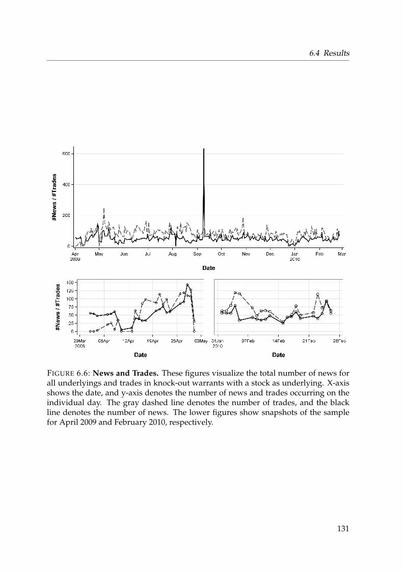
6.4 Results
FIGURE 6.6: News and Trades. These figures visualize the total number of news forall underlyings and trades in knock-out warrants with a stock as underlying. X-axisshows the date, and y-axis denotes the number of news and trades occurring on theindividual day. The gray dashed line denotes the number of trades, and the blackline denotes the number of news. The lower figures show snapshots of the samplefor April 2009 and February 2010, respectively.
131

Chapter 6 Retail Investors’ Trading Behavior
sentiment dummy variables Smt separately for positive (m = 1), negative (m = 2),
and neutral (m = 3) news announcements. They are set to one within a range of
six hours around a positive, negative, and neutral news event, respectively. Let l
denote an observation in my data set, and x denotes the underlying of the product
the observation belongs to. I include dummy variables for the underlying (U), for the
hour of the day (T), and the day of the week (W). Let Mxl denote the trading intensity
measure (#Trades, Volume, #Long, #Short) for underlying x and observation l. The
regression is then modeled as follows:
Mxl = α +2
∑n=1
3
∑m=1
ψnm InxlSmxl +30
∑x=1
υxUx +11
∑t=1
τtTt +4
∑d=1
ωdWd + εx.
I use generalized method of moments (GMM) for the estimation and correct stan-
dard errors for heteroscedasticity effects, and serial correlation using the procedure
proposed by Newey and West (1987). Consequently, I obtain results for the trading
intensity six hours before and after news, relative to periods of no news, and with
respect to the sentiment of news.
Table 6.7 reports results for the above regression model, excluding all control vari-
ables for clarity reasons. As already indicated by Figure 6.6, the number of trades in
knock-out warrants is higher around news events of the underlying. This is in line
with research on ordinary stocks by Riordan et al. (2013), and Berry and Howe (1994).
Overall, I observe positive estimates for all trading intensity measures - ignoring the
net trading measure - around news, except for trading volume before neutral news.
This means that overall trading activity increases around news. The increase in en-
tered short positions compared to long positions seems to be higher before positive
and neutral news, and lower before negative news. However, the difference of long
minus short positions before positive news and before negative news is not signifi-
cant (estimate: 1.97; t-value: 0.58).
To calculate the actual profitability around news events, I calculate for each trade
the difference in time to the next news after the trade that refers to the specific under-
lying stock. I cluster trades by the passing time until the next news event occurs. I
group trades that have been executed within 30 minutes before a news event in the
underlying, between 30 minutes and one hour, one hour and five hours, and between
132

6.4 Results
TAB
LE
6.7:
Ret
ailI
nves
tor
Trad
ing
Inte
nsit
yA
roun
dN
ews.
This
tabl
epr
ovid
esre
sult
sfo
rtr
adin
gin
tens
ity
mea
sure
sar
ound
new
sfo
rre
tail
inve
stor
s.Th
ete
rms
Posi
tive,
Neg
ativ
e,an
dN
eutr
alre
fer
toth
ese
ntim
enta
naly
sis
ofth
eR
eute
rsN
ewsS
cope
Sent
imen
tEn
gine
.Be
fore
and
Afte
rde
note
the
peri
odof
six
hour
sbe
fore
and
afte
rin
divi
dual
new
s.T-
valu
esar
ere
port
edin
pare
nthe
ses.
*/**
/***
deno
tes
sign
ifica
nce
belo
wth
e5%
/1%
,and
0.1%
leve
l,re
spec
tive
ly.
Posi
tive
Neg
ativ
eN
eutr
alBe
fore
Aft
erBe
fore
Aft
erBe
fore
Aft
er
#Tra
des
per
Min
.[×
10k]
9.79
***
7.48
***
12.2
7***
12.3
9***
4.76
**9.
68**
*(6
.50)
(5.3
9)(9
.25)
(9.6
4)(2
.68)
(5.1
6)Vo
lum
epe
rM
in.
2.49
*0.
234.
39**
*4.
22**
*-1
.99
3.90
*(2
.24)
(0.2
3)(3
.76)
(3.7
4)(-
1.32
)(2
.25)
#Lon
gPo
siti
ons
per
Min
.[×
10k]
4.65
***
5.02
***
7.30
***
6.19
***
0.41
6.99
***
(4.5
0)(4
.84)
(6.8
6)(6
.19)
(0.2
8)(4
.51)
#Sho
rtPo
siti
ons
per
Min
.[×
10k]
5.14
***
2.46
**4.
98**
*6.
20**
*4.
35**
*2.
70**
(4.7
4)(2
.70)
(6.4
0)(7
.83)
(4.2
4)(2
.59)
#Lon
g-#
Shor
tPos
itio
nspe
rM
in[×
10k]
-0.5
02.
562.
32-0
.01
-3.9
0*4.
29*
(-0.
33)
(1.8
7)(1
.78)
(-0.
01)
(-2.
24)
(2.3
1)
133

Chapter 6 Retail Investors’ Trading Behavior
five hours and 24 hours. Table 6.8 reports results for the predictive capabilities of
retail investor trades. I exclude all combinations of holding periods and time differ-
ences which would refer to a sell of the position before the time of arrival of the ac-
tual predicted news. Retail investors have a negative performance at all times, which
implies that informational advantages can be ruled out as trading motivation. Raw
returns range from −5.04% to −12.40% for the buy-and-hold approach, and from
−24.38% to −29.15% for my matched sample. Again, transaction costs are causing
negative performance to a large extent.
Summarizing, retail investors are attracted by news events, but have no informa-
tional advantage whatsoever. Due to the leverage of the analyzed products, they
lose substantial amounts of money within a short period of time. Barber and Odean
(2000) argue that such behavior of increased trading activity but poor performance
can be explained through overconfidence of retail investors (see Section 3.2). Another
alternative explanation is the existence of the disposition effect (see Section 3.2). In
case of knock-out warrants, the disposition effect could lead to higher losses com-
pared to stock investments. Investors that are reluctant to realize their losses, which
might even occur within hours or minutes, might suffer from a total loss in the end.
Additionally, the higher leverage of products could lead to a higher misjudgment of
probabilities. As a result, investors could be more optimistic regarding the future re-
turns and, thus, refuse to realize losses. Furthermore, prices of knock-out warrants
very close to the barrier are very small, which might result in an additional gam-
bling effect in the way of "all-or-nothing" for investors. They rather have the chance
of a turn around and, thus, higher profits than to save the residual amount of their
investment.
6.5 Conclusion
Investing should be more like watching paint dry or watching grass grow. If you
want excitement, take $800 and go to Las Vegas.
- Paul Samuelson, Nobel laureate
Several studies have shown that retail investors trade excessively and tend to favor
stocks with lottery-like characteristics (for example: Han and Kumar, 2012; Brunner-
134

6.5 ConclusionTA
BL
E6.
8:N
ews
Trad
ing.
Iana
lyze
for
each
trad
eth
edi
ffer
ence
inti
me
toth
ene
xtne
ws
ahea
d.R
epor
ted
valu
esar
eth
em
ean
rela
tive
perf
orm
ance
[%](
Raw
Ret
.and
w/o
TC)a
ndsh
arpe
rati
o(A
dj.R
et.)
[%]a
cros
sal
ltra
des
diff
eren
tiat
edby
thei
rdi
stan
cein
tim
eto
the
new
saf
ter
(Pre
dict
ion)
the
trad
e.Pe
rfor
man
ceis
mea
sure
dba
sed
ona
mat
ched
sam
ple
asw
ell
asas
sum
ing
abu
y-an
d-ho
ldst
rate
gyfo
rdi
ffer
ent
hori
zons
:30
min
utes
,one
tofo
urtr
adin
gho
urs,
and
one,
two,
and
five
trad
ing
days
.Pe
riod
sex
ceed
ing
trad
ing
hour
sof
ada
yar
eco
ntin
ued
attr
adin
gho
urs
onth
efo
llow
ing
day.
T-va
lues
are
repo
rted
inpa
rant
hese
s.*/
**/*
**de
note
ssi
gnifi
canc
ebe
low
the
5%/1
%,a
nd0.
1%le
vel,
resp
ecti
vely
.M
atch
edBu
y-an
d-H
old
Sam
ple
0.5h
1h2h
3h4h
1d2d
5d
Raw
Ret
urn
t<0.
5h-2
6.11
***
-5.4
0***
-5.5
5***
-5.8
8***
-6.6
4***
-7.4
9***
-9.4
7***
-11.
39**
*-9
.29*
**(-
13.8
0)(-
17.1
8)(-
15.0
8)(-
13.4
5)(-
13.7
6)(-
14.3
7)(-
12.0
5)(-
12.3
7)(-
8.34
)0.
5h≤
t<1h
-29.
15**
*-5
.94*
**-6
.21*
**-7
.04*
**-8
.18*
**-1
1.53
***
-12.
40**
*-1
0.33
***
(-13
.09)
(-12
.38)
(-11
.57)
(-11
.53)
(-11
.16)
(-10
.80)
(-9.
96)
(-6.
70)
1h≤
t<5h
-24.
38**
*-5
.04*
**-5
.82*
**-6
.74*
**-9
.44*
**-1
0.12
***
-7.1
8***
(-19
.04)
(-18
.82)
(-18
.66)
(-19
.04)
(-17
.15)
(-14
.94)
(-8.
37)
5h≤
t<24
h-2
8.72
***
-6.3
2***
-9.1
8***
-6.1
0***
(-27
.42)
(-12
.88)
(-15
.62)
(-8.
19)
w/o
TCt<
0.5h
-21.
26**
*1.
69**
*1.
48**
*1.
06*
0.19
-0.8
7-3
.02*
**-5
.14*
**-3
.03*
(-10
.38)
(4.5
8)(3
.42)
(2.0
7)(0
.35)
(-1.
53)
(-3.
44)
(-5.
03)
(-2.
38)
0.5h≤
t<1h
-24.
63**
*0.
910.
53-0
.42
-1.9
3*-5
.57*
**-6
.47*
**-4
.75*
*(-
10.4
0)(1
.74)
(0.9
1)(-
0.63
)(-
2.47
)(-
4.85
)(-
4.83
)(-
2.86
)1h≤
t<5h
-19.
75**
*1.
59**
*0.
69*
-0.3
6-3
.44*
**-4
.30*
**-1
.36
(-14
.39)
(5.2
7)(2
.01)
(-0.
93)
(-5.
71)
(-5.
84)
(-1.
46)
5h≤
t<24
h-2
4.18
***
0.36
-2.8
8***
0.00
(-21
.57)
(0.6
4)(-
4.44
)(0
.00)
Adj
.Ret
urns
t<0.
5h0.
22-4
.02*
**-3
.15*
**-2
.56*
**-2
.14*
**-1
.75*
**-1
.19*
**-1
.36*
**-0
.68*
**(0
.44)
(-12
.67)
(-11
.86)
(-14
.14)
(-12
.53)
(-15
.05)
(-12
.62)
(-11
.38)
-(7.
54)
0.5h≤
t<1h
-38.
10-2
.86*
**-2
.14*
**-1
.79*
**-1
.97*
**-1
.48*
**-1
.30*
**-0
.73*
**(-
1.06
)(-
7.85
)(-
9.77
)(-
10.7
2)(-
9.61
)(-
9.55
)(-
9.84
)(-
5.76
)1h≤
t<5h
-0.0
3-2
.06*
**-1
.88*
**-1
.81*
**-1
.22*
**-1
.20*
**-0
.68*
**(-
0.13
)(-
17.9
8)(-
15.5
4)(-
14.3
4)(-
15.2
4)(-
13.1
2)(-
9.73
)5h≤
t<24
h3.
99-0
.74*
**-0
.83*
**-0
.40*
**(0
.94)
(-11
.86)
(-12
.65)
(-6.
15)
135
Chapter 6 Retail Investors’ Trading Behavior
meier and Parker, 2007; Garrett and Sobel, 1999; Gao and Lin, 2012). This chapter in-
vestigates the trading behavior of retail investors in a market dedicated to short-term
speculation. German investment banks provide retail investors with the opportunity
to trade highly leveraged products ideally suited to speculate and/or gamble.
I use a two-fold approach to capture retail investor performance on a trade-by-
trade basis. First, I calculate returns for every trade in the sample assuming different
holding periods, ranging from 30 minutes up to 5 days. Second, I adapt an algorithm
based on backend data of Stuttgart Stock Exchange to match buy and sell orders com-
ing from the same routing provider/broker and, thus, retrieve actual holding periods
for the majority of the total sample.
I find that retail investors’ performance strongly depends on the underlying type
of the investment: Index or stocks. They have a positive return if they speculate on
mid term index movements, and a negative return when speculating on single con-
stituents or intraday index movements. However, risk-adjusted returns show that
overall investment strategies involving knock-out warrants perform badly on a risk-
adjusted basis. Negative performance of retail investors is largely driven by trans-
action costs. Transaction costs reduce wealth of investors by approximately 6% on
average.
Trading intensity of retail investors in products with a stock as underlying in-
creases around news. However, retail investors do not have any informational ad-
vantage and no predictive power whatsoever.
Products with extreme returns for ’correct bets’ seem to greatly attract speculators
and gamblers. It seems that investors are more or less decreasing their wealth to
indulge in the adrenaline of trading highly leveraged products.
136

Chapter 7
Conclusion and Future Research
”[There] are questions that many investors simply may not ask because we are humans, not
automatons. Susceptible to behavioural biases, to framing, to anchoring, to poor decision
making. Regulators need to have the power and expertise - the remit - to anticipate these
influences and react to them.”
Martin Wheatley (Chief Executive of the Financial Conduct Authority)
7.1 Contributions
STRUCTURED products have been a huge innovative step in financial markets,
allowing retail investors to act in dimensions that have not been possible before.
Speculating on falling, rising, or sideways markets with linear or disproportional
payoffs on commodities, stocks, or currencies. Retail investors have been given the
possibility to trade on almost everything they can imagine.
I studied structured products along several dimensions with a focus on the Ger-
man market. Particularly, I examined both issuers of structured products and in-
vestors trading them, as addressed in the following two research questions:
• Do issuers exploit the ignorance of retail investors?
137

Chapter 7 Conclusion and Future Research
• Is trading in structured products beneficial for retail investors wealth?
Based on the analyses contained in this thesis, answers to these questions can be given
briefly as follows.
Contribution 1: Do issuing investment banks exploit the ignorance of retail in-
vestors? Over the last years several studies on structured products across different
European markets and the US have addressed facets of this question. Overall, they all
find that investment banks, which issue products designed for retail investors, add
a significant surplus on theoretical fair prices of their products. First, I verify this
phenomena for the German market for several product types. The premium, i.e. the
difference between observed quoted prices by issuers and theoretical prices, strongly
depends on the specific product type and issuer. Second, I analyze several factors that
influence the degree of overpricing by issuers. The work at hand provides evidence
that issuers pricing policies are influenced by timing factors, such as, the hour of the
day, the remaining life time of the product, the demand of retail investors, and the
complexity of the product type. Issuers increase their overpricing towards the end
of a trading day, and in times of high uncertainty. In addition, I find that investment
banks reduce premiums over the life time of their products to achieve additional ben-
efits on the expense of their customers. An in-depth analysis with respect to the de-
mand of investors on an individual trade level reveals that issuers adjust their quoted
prices after executed orders. I observe a positive effect on premiums when shares are
bought, and a negative impact when shares are sold. One interpretation for this is that
investment banks increase premiums when they expect buy orders to dominate, and
decrease premiums when sell orders seem to dominate. Finally, products that are
observed to be more complex due to their inherent option structure include higher
premiums compared to those, which are easier to understand.
Contribution 2: Is trading in structured products beneficial for retail investors
wealth? With the introduction of structured products, issuers provide retail in-
vestors with great opportunities to participate in stock, FX, and commodity markets.
By means of the liquidity provision of issuers and, thus, the easy way of buying and
selling specifically designed products for every market movement, investors may feel
138

7.2 Regulatory Proposals and Implications
like professional traders, having theoretically the possibility to achieve fortunes in a
short time. However, data of leveraged trading analyzed in this thesis offers a pic-
ture that distorts the illusion of retail investors actually behaving like professionals.
Although, retail investors trading activity increases around news, i.e. when new in-
formation becomes available, analyzing the performance of their trades leads to the
conclusion that, in fact, retail investors do not make profits but rather experience
heavy losses on average. Such losses are driven to a large extent by implicit and ex-
plicit transaction costs. It remains unclear whether investors trade to meet their need
of entertainment and gambling, which might compensate them for their losses, or if
they actively pursue an increase of their wealth, which just does not work out in their
favor. Nevertheless, analyzing retail investor trades with respect to the assumed risks
reveals poor investments on average. Investors expose themselves, i.e. their wealth,
to great risks to realize potential profits.
Whether the regulator should step in to protect investors from losing money due to
their own misplaced actions and, to a smaller extent, the service charge in form of the
premium is not for me to judge. However, the following section provides suggestions
which could increase the overall reputation of the market for structured products.
7.2 Regulatory Proposals and Implications
This section presents regulatory suggestions to increase transparency and fairness of
the market for structured products.
7.2.1 Obligation to Provide Full Transparency
Currently, regulators are debating whether issuers should disclose hidden fees and
fair prices of their own products.1 Although, such an approach would increase the
transparency of the market substantially, it remains a difficult task to formalize rules
that would prevent issuers from hiding margins in their products. For example, ad-
justing the volatility parameter in pricing formulas has a huge direct impact on prices
1See http://www.iosco.org/library/pubdocs/pdf/IOSCOPD410.pdf. Accessed06/26/2013.
139

Chapter 7 Conclusion and Future Research
and, thus, can be used as a lever to control prices without actually adding an explicit
fee. There is no rule that defines the explicit calculation of the implied volatility or
any other involved parameter, which still leaves room for the incorporation of hidden
margins. An enforcement of such an approach is therefore rather difficult.
In my opinion, providing more insight information on costs from an issuer per-
spective would be helpful and increase transparency, but it does not solve problems
that actually matter for most investors. A slightly reduced margin does not compen-
sate for overall bad investments that arise through improper use of products due to
underestimation of risks and cognitive biases.
As long as structured products are issued as bearer bonds, it is practically impos-
sible for banks to provide liquidity for products of their competitors. Therefore, no
direct price competition arises in structured products. Instead of enforcing fair prices,
the following approach tries to increase price efficiency through increased competi-
tion.
7.2.2 Standardization
In Section 5.4.5, I provide evidence that, although, the number of tradable products
is large, products are not directly comparable to each other. Due to the complexity of
the component structure and the non-linear pricing of barrier options, products that
do not have the same characteristics are hardly comparable. This leads to obfusca-
tion in the market and allows for higher premiums. However, if the regulator would
define a strict issuance grid for each underlying type that only allows for specific com-
binations market transparency could be increased. Issuers would be forced to issue
identical products in order to compete for order flow. Figure 7.1 briefly visualizes a
sample issuance grid for warrants with DAX30 as underlying. Investment banks are
allowed to issue products on every 50 points of the index starting from 0 up to 15,000
points. Maturity dates for products are fixed on specific dates, for example at the end
of each quarter. Issuers are allowed to issue their products continuously, but still with
respect to the fixed maturity dates. As a result, issuing endless products, i.e. with no
maturity date, would not be possible anymore. The frequent adjustments of product
characteristics and the hard to understand methodology behind it makes it nearly
140

7.2 Regulatory Proposals and Implications
FIGURE 7.1: Issuance Grid. This figure sketches an issuance grid for warrants desig-nated on the DAX.
impossible for retail investors to assess a good investment opportunity. As a result,
products of different issuers would be more comparable with each other. This could
lead to more efficient prices from an investor perspective and, thus, reduce margins
without interfering with issuers’ pricing models.
However, since the default risk of the issuer is a substantial driving factor for
prices of structured products, prices of products with the same characteristics but
different issuers might still deviate from each other. Banks with the highest default
risk should offer "the cheapest" products from an investor’s perspective. Although,
all issuers might price their products equally fair, investors could simply focus on the
smallest absolute price and order flow is concentrated on the issuer with the high-
est default risk as a result. Additionally, employing an issuance grid results in a
smaller product variety and less possibilities for investors to exactly match their ex-
pectations.
7.2.3 Ban of Highly Complex Products
The Financial Services and Markets Authority (FSMA), a Belgian financial regulator,
calls distributors of structured products to take part in a moratorium for "particularly
complex products"2. All signers oblige themselves to not issue products after Au-
2A "particularly complex product" is a product that does not meet at least one of the following fourcriteria: (i) "the underlying value is sufficiently accessible and transparent to the consumer", (ii) "theinvestment strategy is not overly complex", (iii) "the yield is not calculated on the basis of morethan three mechanisms", and (iv) there is "transparency regarding costs, credit risk and market
141

Chapter 7 Conclusion and Future Research
gust 1, 2011 that fall in the category "particularly complex products". Several other
European regulators are discussing product intervention, focusing either on rules for
banning products or extended information disclosure. One can reasonably assume
that retail investors are not able to understand very complex products in detail, i.e.
their pricing mechanisms, but nevertheless they are informed by the issuing bank and
resellers of the purpose of the product. Whether this is sufficient to allow investors to
trade them remains beyond the scope of this thesis.
7.3 Outlook
While important questions on the German market of structured products have been
addressed in this thesis, several aspects remain yet unsolved and, thus, may provide
possible avenues for future research. Some of them are briefly discussed in the fol-
lowing.
Hidden margins in exotic structured products
This thesis has addressed several major product types in the German market. How-
ever, there is only very limited literature that refers to more exotic product types with
highly complex payoff structures. Due to considerable obstacles, such as missing
information on internal product characteristics, the calculation of theoretical prices is
highly challenging and, thus, provides the ideal environment for a fuzzy pricing of is-
suers. While many of those products are traded by retail investors, it is still unknown
whether investors are being exploited and, if so, to which extent.
Differences in overpricing between regulated markets and over-the-counter
markets
Academic literature almost solely refers to the analysis of prices on regulated mar-
kets, i.e. on designated trading segments at exchanges. However, OTC markets usu-
ally offer a cheaper (in terms of explicit transaction costs) execution throughout the
value". Quotations and a more detailed definition of products that fall under the moratorium can befound here: http://www.fsma.be/en/in-the-picture/Article/nipic/faqa.aspx#4.Accessed 07/18/2013.
142
7.3 Outlook
day. Additionally, trading hours are extended compared to regulated markets. So far
there are almost no empirical studies whether prices at OTC markets and regulated
markets are different from each other. Since most turnover in German structured
products is generated in OTC markets this question is highly relevant for retail in-
vestors.3
Sensitivity of retail investors to hidden margins
As already pointed out above, current political debates discuss the disclosure of hid-
den margins incorporated in product prices. Capturing the sensitivity of retail in-
vestors towards inherent costs could provide insights for future regulatory initiatives
concerning hidden costs. Additionally, it would be of interest to examine whether
investors experience any learning effects regarding inherent costs of products. Prod-
ucts offering better prices would attract more order flow compared to worse priced
products of competitors. Thus, investors may provide independently a better envi-
ronment for an enhanced price competition between different issuers.
Technical trading as motivation for trades in leverage products
Pattern recognition and chart tools are becoming increasingly popular among retail
investors, being provided on all major financial information portals. Many internet
sources offer financial advice based on technical analysis presenting a source of infor-
mation for retail investors. It is of great interest whether retail investors use technical
analysis as one of the main sources of information. Due to the excessive amount of
HFT trading in stock markets, trading on technical patterns might be a substantial
source of misguided trades. HFT are easily able to use momentum effects to push
prices in a desired direction to pick up uninformed small investors.
Investor comprehension and investor decision
Another avenue for future research is the interaction between financial literacy and
investment decisions. This could include correct understanding of product risks,
3There are no publicly available statistics regarding the actual turnover of OTC markets versus regu-lated exchanges. However, according to professional traders at Stuttgart Stock Exchange the shareof OTC turnover relative to the total turnover ranges approximately between 70%-80% in Germany.
143

Chapter 7 Conclusion and Future Research
expected returns, and influencing parameters. To which extent are retail investors’
choices of investing into structured products influenced by a lack of financial literacy?
Are products still attractive if all risks are understood and costs are fully disclosed?
7.4 Summary
In this chapter, I have presented my major contributions to the literature, based on
the work at hand. There is significant evidence that issuers systematically abuse their
monopolistic power of quoting prices to gain profits on expenses of retail investors.
However, whether or not this extents the benefit some investors might see in those
products is left to those who have actually traded them. As for my sample and ob-
servation period, I can conclude that retail investors, on average, reduce their wealth
significantly by speculating with leverage products.
Based on the results in this thesis, I outlined several suggestions for regulators to
increase transparency and market efficiency, which includes banning highly complex
products and the introduction of a standardized issuance grid for issuers.
Additionally, I have outlined several opportunities for future research to establish
a better understanding of the market for structured products. Besides extended anal-
yses on the hidden product premium and its differences between trading venues,
a major future focus of research may lie on the interaction of financial literacy and
investor decision making.
144

Appendix A
List of Abbreviations
A.1 List of Abbreviations
BaFIN Bundesanstalt für Finanzdienstleistungsaufsicht (German Financial
Supervisory Authority) . . . . . . . . . . . . . . . . . . . . . . . . . . . . . . . . . . . . . . . . . . . . . . . . . . . . . . . . . 22
BGB Bürgerliches Gesetzbuch (German Civil Code) . . . . . . . . . . . . . . . . . . . . 22
BörsG Börsengesetz (Stock Exchange Act) . . . . . . . . . . . . . . . . . . . . . . . . . . . . . . . . 23
DAX Deutscher Aktienindex . . . . . . . . . . . . . . . . . . . . . . . . . . . . . . . . . . . . . . . . . . . . 38
DDV Deutscher Derivateverband (German Derivatives Association) . . . . 13
EOD End-of-Day . . . . . . . . . . . . . . . . . . . . . . . . . . . . . . . . . . . . . . . . . . . . . . . . . . . . . . . 54
EUREX European Exchange . . . . . . . . . . . . . . . . . . . . . . . . . . . . . . . . . . . . . . . . . . . . . . . 14
EURIBOR Euro Interbank Offered Rate . . . . . . . . . . . . . . . . . . . . . . . . . . . . . . . . . . . . . . 69
EUSIPA European Structured Investment Products Association . . . . . . . . . . . . 16
EUWAX European Warrant Exchange . . . . . . . . . . . . . . . . . . . . . . . . . . . . . . . . . . . . . . 11
FCA Financial Conduct Authority . . . . . . . . . . . . . . . . . . . . . . . . . . . . . . . . . . . . . . . 3
FESE Federation of European Securities Exchanges . . . . . . . . . . . . . . . . . . . . . . 10
FSMA Financial Services and Markets Authority . . . . . . . . . . . . . . . . . . . . . . . . 141
FX Foreign Exchange Market . . . . . . . . . . . . . . . . . . . . . . . . . . . . . . . . . . . . . . . . 138
GMM Generalized Method of Moments . . . . . . . . . . . . . . . . . . . . . . . . . . . . . . . . 132
HFT High-Frequency Trading . . . . . . . . . . . . . . . . . . . . . . . . . . . . . . . . . . . . . . . . . . 24
IOSCO International Organization of Securities Commissions . . . . . . . . . . . . . 42
ISIN International Securities Identification Number . . . . . . . . . . . . . . . . . . . . . 55
KID Key Information Documents . . . . . . . . . . . . . . . . . . . . . . . . . . . . . . . . . . . . . . 23
I

Appendix A List of Abbreviations
KIT Karlsruhe Institute of Technology . . . . . . . . . . . . . . . . . . . . . . . . . . . . . . . . . . a
NDX Nordic Derivatives Exchange . . . . . . . . . . . . . . . . . . . . . . . . . . . . . . . . . . . . . 29
MiFID Markets in Financial Instruments Directive . . . . . . . . . . . . . . . . . . . . . . . . 23
NYSE New York Stock Exchange . . . . . . . . . . . . . . . . . . . . . . . . . . . . . . . . . . . . . . . . 43
OCO One-cancels-the-other order . . . . . . . . . . . . . . . . . . . . . . . . . . . . . . . . . . . . . . 110
OTC Over-The-Counter . . . . . . . . . . . . . . . . . . . . . . . . . . . . . . . . . . . . . . . . . . . . . . . . 11
PBS Practitioners Black-Scholes . . . . . . . . . . . . . . . . . . . . . . . . . . . . . . . . . . . . . . . . 60
PNAC Primary News Access Code . . . . . . . . . . . . . . . . . . . . . . . . . . . . . . . . . . . . . . . 58
PRIP Packaged Retail Investment Products . . . . . . . . . . . . . . . . . . . . . . . . . . . . . 23
RIC Reuters Information Code . . . . . . . . . . . . . . . . . . . . . . . . . . . . . . . . . . . . . . . . . 54
RNSE Thomson Reuters NewsScope Sentiment Engine . . . . . . . . . . . . . . . . . . . 58
SchVG Schuldverschreibungsgesetz (Debenture Bond Act) . . . . . . . . . . . . . . . . 22
SIRCA Securities Industry Research Centre of Asia Pacific . . . . . . . . . . . . . . . . 54
S&P 500 Standard & Poor’s 500 . . . . . . . . . . . . . . . . . . . . . . . . . . . . . . . . . . . . . . . . . . . . 35
SPARQS Stock Participating Accreting Redemption Quarterly-Pay Securities 38
TAQ Trade and quote . . . . . . . . . . . . . . . . . . . . . . . . . . . . . . . . . . . . . . . . . . . . . . . . . . . 54
TRDTH Thomson Reuters DataScope Tick History . . . . . . . . . . . . . . . . . . . . . . . . . 53
TRNA Thomson Reuters News Analytics . . . . . . . . . . . . . . . . . . . . . . . . . . . . . . . . . 58
WKN Wertpapierkennnummer . . . . . . . . . . . . . . . . . . . . . . . . . . . . . . . . . . . . . . . . . . 55
WpDVerOV Verordnung zur Konkretisierung der Verhaltensregeln und Organisa-
tionsanforderungen für Wertpapierdienstleistungsunternehmen . . . . . . . . . . . . . . . . . 22
WpHG Wetpapierhandelsgesetz (Securities Trading Act) . . . . . . . . . . . . . . . . . . 23
WpPG Wertpapierprospektgesetz (Securities Prospectus Act) . . . . . . . . . . . . . 22
II

Appendix B
German Product Classification
The following table shows the product classification for the German market of struc-
tured products according to the German Derivatives Association. The names and
descriptions are extracted without changes from DDV.1 The classification does not
capture all product types tradable in Germany. There are many exotic products that
do not fit in the classification scheme. However, trading volume in exotic products is
negligible.
1http://www.deutscherderivateverband.de/MediaLibrary/Document/Derivate-Liga_A3_2013_EN.pdf. Accessed 2013/24/06.
III

Appendix B German Product Classification
TABLE B.1: German Classification for Structured ProductsName Description
Investment ProductsCapital Protection Prod-ucts with Coupon
Capital Protection Products with Coupon are interest-bearing securi-ties with various additional conditions attached. The amount of inter-est may depend on the performance of the underlying asset. At finalmaturity the bonds offer 100 percent capital protection
Uncapped Capital Protec-tion Certificates
With Uncapped Capital Protection Certificates, the issuer promises torepay the nominal amount to the investor at maturity. In addition,there is the potential for attractive returns depending on the perfor-mance of one or several underlyings
Reverse Convertibles With reverse convertibles, interest is paid regardless of the perfor-mance of the underlying asset. The type and the amount of the re-payment at final maturity depend on whether the value of the un-derlying asset is equal to, or above or below the strike price on thevaluation date. If the value of the underlying asset at the valuationdate is at least equal to the strike price, the investor receives the nom-inal value. If the value of the underlying asset is below the strikeprice, the investor receives either the value of the underlying asset orthe underlying assets themselves
Credit Linked Notes Credit Linked Notes offer a means of investing in a borrower’s creditrating. The amount of interest and the capital repayment are depen-dent on the borrower’s credit rating. As long as the borrower does notexperience a credit event, the investor will receive interest paymentsand,when the note matures, the nominal value. If a credit event doesoccur, however, the note is repaid early. In this case, interest pay-ments cease, and the amount repaid may be significantly below thenominal value
Discount Certificates Discount Certificates give a discount on the current price of the un-derlying. This discount provides a cushion against potential falls inthe price of the underlying. In return, investors accept a cap on profitsfrom potential price rises, and they do not receive any dividends
Express Certificates With Express Certificates, movements in the price of the underlyingare monitored at specific intervals (e.g. annually) and compared withthe initial price. If, at one of the reference dates, the price is higherthan the initial price, the investor receives the nominal value of thecertificate plus a predefined additional amount before the end of theterm. If the price is not higher than the initial price at the referencedate, the process is repeated in the next period taking double the ad-ditional amount as a basis, and so on. If the price falls, a cushiongenerally absorbs any price falls up to a predefined value. It is onlyif the price falls below this predefined value that losses will arise, asthey would with a direct investment in the underlying asset
Bonus Certificates Bonus Certificates pay a bonus amount at final maturity if the un-derlying does not reach or breach the specified barrier in the relevantmonitoring period. The investor does not receive any dividend pay-ments
IV

TABLE B.1: continuedName Description
Tracker Certificates Tracker Certificates offer exposure to the movements in the price ofan underlying instrument. This means that with just one certificate,investors can put their money into an asset class, sector or region,optimizing and diversifying their portfolio
Outperformance /Capped Outerperfor-mance Certificates
With Outperformance Certificates, if the price of the underlying assetgoes up, investors receive a return equal to a pre-specified multiple ofthe return on the underlying asset. Capped Outperformance Certifi-cates offer investors the opportunity for leveraged profit from a risein the price of the underlying above the strike price within a specifiedrange. The profit is limited by a cap. With products of this type, theinvestor’s exposure to potential losses below the strike price is limitedto any loss in the underlying. There is no entitlement to a dividend
Leverage ProductsWarrants Warrants provide leveraged exposure to rising (call) and falling (put)
prices in an underlying. The price is influenced not only by move-ments in the underlying, but also by other factors such as volatility orthe (residual) term. If the price of the underlying at maturity is below(call) or above (put) the strike price, investors lose their entire capital
Factor Certificates Factor Certificates provide leveraged exposure to both rising (long)and falling (short) prices in an underlying asset. They have no fixedterm and are based on a strategy index that reflects the percentagedaily change in the underlying using a constant factor. The size of thefactor determines the amount by which the strategy index leveragesthe daily price change in the underlying
Knock-Out Warrants Like Warrants, Knock-Out Warrants also provide leveraged exposureto rising (call) and falling (put) prices in an underlying. Knock-outwarrants track the movements of the underlying on a one-to-one ba-sis. This largely eliminates the impact of volatility. If the knock-outbarrier is breached, investors generally lose all their invested capital
V

Appendix B German Product Classification
VI

Appendix C
Sample Data - Thomson Reuters
DataScope Tick History
VII

Appendix C Sample Data - Thomson Reuters DataScope Tick History
TAB
LE
C.1
:Tho
mso
nR
eute
rsD
ataS
cope
Tick
His
tory
-Int
rada
ySa
mpl
eR
ICD
ate
Tim
eG
MT
Off
set
Type
Ope
nH
igh
Low
Last
AD
SG.D
E02
-MA
R-2
009
08:0
2:00
.000
1In
trad
ay1M
in22
.41
22.8
122
.41
22.6
AD
SG.D
E02
-MA
R-2
009
08:0
3:00
.000
1In
trad
ay1M
in22
.63
22.6
722
.59
22.6
7A
DSG
.DE
02-M
AR
-200
908
:04:
00.0
001
Intr
aday
1Min
22.6
522
.66
22.6
522
.66
AD
SG.D
E02
-MA
R-2
009
08:0
5:00
.000
1In
trad
ay1M
in22
.68
22.7
222
.67
22.6
7A
DSG
.DE
02-M
AR
-200
908
:06:
00.0
001
Intr
aday
1Min
22.6
122
.61
22.6
122
.61
AD
SG.D
E02
-MA
R-2
009
08:0
7:00
.000
1In
trad
ay1M
in22
.622
.622
.52
22.5
2A
DSG
.DE
02-M
AR
-200
908
:08:
00.0
001
Intr
aday
1Min
22.6
22.6
122
.54
22.5
8A
DSG
.DE
02-M
AR
-200
908
:09:
00.0
001
Intr
aday
1Min
22.6
122
.61
22.5
822
.58
AD
SG.D
E02
-MA
R-2
009
08:1
0:00
.000
1In
trad
ay1M
in22
.58
22.5
822
.58
22.5
8A
DSG
.DE
02-M
AR
-200
908
:11:
00.0
001
Intr
aday
1Min
22.5
922
.59
22.5
622
.56
AD
SG.D
E02
-MA
R-2
009
08:1
2:00
.000
1In
trad
ay1M
in22
.55
22.5
622
.55
22.5
6A
DSG
.DE
02-M
AR
-200
908
:13:
00.0
001
Intr
aday
1Min
..
..
AD
SG.D
E02
-MA
R-2
009
08:1
4:00
.000
1In
trad
ay1M
in22
.55
22.5
522
.55
22.5
5A
DSG
.DE
02-M
AR
-200
908
:15:
00.0
001
Intr
aday
1Min
22.5
822
.58
22.5
822
.58
AD
SG.D
E02
-MA
R-2
009
08:1
6:00
.000
1In
trad
ay1M
in22
.58
22.6
122
.58
22.6
AD
SG.D
E02
-MA
R-2
009
08:1
7:00
.000
1In
trad
ay1M
in22
.61
22.6
222
.56
22.6
2A
DSG
.DE
02-M
AR
-200
908
:18:
00.0
001
Intr
aday
1Min
..
..
AD
SG.D
E02
-MA
R-2
009
08:1
9:00
.000
1In
trad
ay1M
in.
..
.A
DSG
.DE
02-M
AR
-200
908
:20:
00.0
001
Intr
aday
1Min
22.5
722
.57
22.5
722
.57
AD
SG.D
E02
-MA
R-2
009
08:2
1:00
.000
1In
trad
ay1M
in22
.57
22.6
222
.57
22.6
1A
DSG
.DE
02-M
AR
-200
908
:22:
00.0
001
Intr
aday
1Min
22.5
922
.62
22.5
922
.62
AD
SG.D
E02
-MA
R-2
009
08:2
3:00
.000
1In
trad
ay1M
in22
.61
22.6
422
.61
22.6
4A
DSG
.DE
02-M
AR
-200
908
:24:
00.0
001
Intr
aday
1Min
22.6
122
.61
22.6
22.6
AD
SG.D
E02
-MA
R-2
009
08:2
5:00
.000
1In
trad
ay1M
in22
.62
22.6
522
.61
22.6
1A
DSG
.DE
02-M
AR
-200
908
:26:
00.0
001
Intr
aday
1Min
22.6
122
.61
22.6
22.6
1A
DSG
.DE
02-M
AR
-200
908
:27:
00.0
001
Intr
aday
1Min
22.6
522
.722
.65
22.6
7A
DSG
.DE
02-M
AR
-200
908
:28:
00.0
001
Intr
aday
1Min
22.6
522
.79
22.6
522
.78
AD
SG.D
E02
-MA
R-2
009
08:2
9:00
.000
1In
trad
ay1M
in22
.78
22.8
22.7
522
.8A
DSG
.DE
02-M
AR
-200
908
:30:
00.0
001
Intr
aday
1Min
22.7
622
.822
.75
22.8
VIII

TAB
LE
C.2
:Tho
mso
nR
eute
rsD
ataS
cope
Tick
His
tory
-End
-Of-
Day
Sam
ple
RIC
Dat
eTi
me
Type
Qua
lifier
sO
pen
Hig
hLo
wLa
stVo
lum
e
AD
SG.D
E01
-OC
T-20
09En
dO
fDay
36.4
336
.45
35.4
835
.579
4121
AD
SG.D
E02
-OC
T-20
09En
dO
fDay
35.2
35.6
734
.67
34.9
112
7335
0A
DSG
.DE
03-O
CT-
2009
End
OfD
ayN
oTr
ades
..
..
.A
DSG
.DE
04-O
CT-
2009
End
OfD
ayN
oTr
ades
..
..
.A
DSG
.DE
05-O
CT-
2009
End
OfD
ay35
.01
35.3
334
.71
35.0
456
8638
AD
SG.D
E06
-OC
T-20
09En
dO
fDay
35.6
136
.735
.61
3616
7111
0A
DSG
.DE
07-O
CT-
2009
End
OfD
ay35
.89
36.3
934
.98
35.1
314
9133
1A
DSG
.DE
08-O
CT-
2009
End
OfD
ay35
.235
.48
34.2
534
.527
9234
2A
DSG
.DE
09-O
CT-
2009
End
OfD
ay34
.26
3534
.26
34.8
513
6648
1A
DSG
.DE
10-O
CT-
2009
End
OfD
ayN
oTr
ades
..
..
.A
DSG
.DE
11-O
CT-
2009
End
OfD
ayN
oTr
ades
..
..
.A
DSG
.DE
12-O
CT-
2009
End
OfD
ay35
.15
35.3
934
.734
.75
1056
807
AD
SG.D
E13
-OC
T-20
09En
dO
fDay
34.5
134
.88
34.2
334
.31
1220
124
AD
SG.D
E14
-OC
T-20
09En
dO
fDay
34.7
135
.97
34.7
135
.76
2103
105
AD
SG.D
E15
-OC
T-20
09En
dO
fDay
35.9
536
.44
35.7
836
.312
7028
5A
DSG
.DE
16-O
CT-
2009
End
OfD
ay36
.43
36.6
936
.05
36.1
519
6582
3A
DSG
.DE
17-O
CT-
2009
End
OfD
ayN
oTr
ades
..
..
.A
DSG
.DE
18-O
CT-
2009
End
OfD
ayN
oTr
ades
..
..
.A
DSG
.DE
19-O
CT-
2009
End
OfD
ay36
.436
.736
.29
36.6
9494
38A
DSG
.DE
20-O
CT-
2009
End
OfD
ay36
.95
36.9
535
.735
.81
1388
432
AD
SG.D
E21
-OC
T-20
09En
dO
fDay
35.6
535
.78
34.8
535
.27
2198
390
AD
SG.D
E22
-OC
T-20
09En
dO
fDay
34.9
535
.17
34.6
734
.97
1007
232
AD
SG.D
E23
-OC
T-20
09En
dO
fDay
35.2
935
.64
34.5
434
.789
2444
AD
SG.D
E26
-OC
T-20
09En
dO
fDay
34.9
935
.333
.68
33.7
314
7466
4A
DSG
.DE
27-O
CT-
2009
End
OfD
ay33
.85
34.0
633
.27
33.4
1408
850
AD
SG.D
E28
-OC
T-20
09En
dO
fDay
33.2
533
.43
32.1
132
.15
1880
985
AD
SG.D
E29
-OC
T-20
09En
dO
fDay
32.3
333
.19
32.2
532
.76
1926
726
AD
SG.D
E30
-OC
T-20
09En
dO
fDay
32.9
833
.73
31.3
531
.525
2954
9A
DSG
.DE
31-O
CT-
2009
End
OfD
ayN
oTr
ades
..
..
.A
DSG
.DE
01.N
ov09
End
OfD
ayN
oTr
ades
..
..
.
IX

Appendix C Sample Data - Thomson Reuters DataScope Tick History
X

Appendix D
Sample Data - Stuttgart Stock
Exchange Data
Data descriptions are derived from Boerse Stuttgart (2012).
XI

Appendix D Sample Data - Stuttgart Stock Exchange Data
TABLE D.1: Stuttgart Stock Exchange - Master Data DescriptionVariable Description
Type Product type (AZE = Certificates, WAR = Warrants, KO = Knock-out products,EXO= Exotic products, AKA = Bonds)Format: StringLength: 3
OptionType Option type of the security (call/put).Format: StringLength: 4
IssuerName Name of the issuing bank.Format: StringLength: 50
WKN A German identification code (Wertpapierkennnumber).Format: StringLength: 6
ISIN International Securities Identification NumberFormat: StringLength: 12
ExerciseType Execution type (e=European, a=American)Format: CharacterLength: 1
Underlying ISIN of the underlying security.Format: StringLength: 12
StrikePrice Strike price of a derivative.Format: RealLength: 25
Currency Currency of quoted prices (e.g. EUR = EURO)Format: StringLength: 25
ExpirationDate Expiration day of the security. If endless, value is not set.Format: TT.MM.YYYYLength: 10
SubscriptionRatio Numeric value which represents the subscription ratio when referring toderivative instruments.Format: RealLength: 10
ProductName Official name of the financial instrument as given by the issuer.Format: StringLength: 50
FirstTradingDay First trading day of the security on Stuttgart Stock Exchange.Format: TT.MM.YYYYLength: 10
LastTradingDay Last trading day of the security on Stuttgart Stock Exchange.Format: TT.MM.YYYYLength: 10
XII

TABLE D.1: continuedVariable Description
Description Contains the security description. Usually, in German.Format: StringLength: 200
Cap Some securities have a upper or lower threshold for its payoff pro-file. The threshold value is called Cap.Format: RealLength: 25
SecurityLevel Denotes the barrier level of a financial product.Format: RealLength: 25
KnockOutBarrier Denotes the knock-out barrier level of a financial product. Usually,this field is a substitute to SecurityLevel.Format: RealLength: 25
InterestRate Interest rate for regular defined payments.Format: RealLength: 25
Rolling Indication whether the issuer rolls characteristics such as theknock-out barrier of the financial instrument (j=yes, n=no).Format: CharacterLength: 1
PercentageQuotation Provides information whether the product is noted in percent(n=no, j=yes). If so, sizes of order data are multiplied by 100Format: CharacterLength: 1
SecurityLevelValidFrom Starting date of validity of the security level.Format: TT.MM.YYYYLength: 10
BonusLevel Numeric value for the bonus level of bonus certificates.Format: RealLength: 25
DateOfPayment Date when issuer resolve the payoff of a financial instrument.Format: TT.MM.YYYYLength: 10
XIII

Appendix D Sample Data - Stuttgart Stock Exchange Data
TABLE D.2: Stuttgart Stock Exchange - Order Data DescriptionVariable Description
Ordernumber An integer number which serves as unique identifier for each order sent toStuttgart Stock Exchange. The order number remains the same as long theorder is valid.Format: IntegerLength: 12
Timestamp Date and time of the status change of the order.Format: YYYY-MM-DD hh:mm:ss.sssLength: 23
Code A integer number which defines the status of the order.Format: Integer (001: submission, 003: modification, 005: cancellation, 011:execution)Length: 3
ISIN International Securities Identification Number. Allows for identification of thetraded product.Format: StringLength: 12
Buysell A character that defines a buy (K) or sell (V) order.Format: CharacterLength: 1
Size A real number which represents the submitted number of shares of the order.It is not necessary equal to the number of executed shares.Format: RealLength: 20
Limit A real number which stands for the limit price of the submitted order. De-pending on the trade direction this either results in a minimum or maximumprice threshold for the trade execution.Format: RealLength: 20
Tradeprice A number which identifies the execution price of the order. It is set to NULLfor orders with status unequal 011.Format: RealLength: 20
Tradequantity A number which identifies the number of executed shares.Format: RealLength: 20
RoutingID A number which identifies the routing provider of the order.Format: IntegerLength: 4
XIV

TAB
LE
D.3
:Stu
ttga
rtSt
ock
Exch
ange
-Ord
erD
ata
Sam
ple
Ord
ernu
mbe
rTi
mes
tam
pC
ode
ISIN
WK
NBu
ysel
lSi
zeLi
mit
Trad
epri
ceTr
adeq
uant
itiy
9110
2395
1953
4011
9.66
313
11D
E000
CM
30G
V6
CM
30G
VN
ULL
NU
LLN
ULL
0.61
1000
0091
1024
3129
0840
119.
6631
35
DE0
00D
B90V
42D
B90V
4N
ULL
2720
0N
ULL
NU
LLN
ULL
9110
2395
1959
4011
9.66
313
1D
E000
CM
05SV
3C
M05
SVV
394
0N
ULL
NU
LL91
1023
9519
5740
119.
6631
411
DE0
00C
G05
1E6
CG
051E
NU
LLN
ULL
NU
LL3.
5210
0091
1024
3128
7140
119.
6631
45
DE0
00D
B54S
M1
DB5
4SM
NU
LL20
000
NU
LLN
ULL
NU
LL91
1023
8049
3240
119.
6631
51
DE0
00BN
7CP4
0BN
7CP4
V70
00
NU
LLN
ULL
9110
2910
1610
4011
9.66
315
1D
E000
CM
325Z
1C
M32
5ZK
500
2.2
NU
LLN
ULL
9110
2425
0729
4011
9.66
316
5D
E000
DB6
9DQ
2D
B69D
QN
ULL
2000
0N
ULL
NU
LLN
ULL
9110
2405
2580
4011
9.66
316
1D
E000
PAH
0038
PAH
003
V10
052
.5N
ULL
NU
LL91
1023
9519
5940
119.
6631
711
DE0
00C
M05
SV3
CM
05SV
NU
LLN
ULL
NU
LL9.
7639
491
1027
3013
1240
119.
6631
711
XS0
4102
9935
7EN
AG
0SN
ULL
NU
LLN
ULL
106.
8350
000
9110
2390
2865
4011
9.66
318
1N
L000
0118
024
6142
25V
1000
0N
ULL
NU
LL91
1024
2056
2440
119.
6631
85
DE0
00D
B16T
05D
B16T
0N
ULL
3000
NU
LLN
ULL
NU
LL91
1024
2095
8540
119.
6631
85
DE0
00D
B8V
X39
DB8
VX
3N
ULL
1000
NU
LLN
ULL
NU
LL91
1023
8049
3240
119.
6631
911
DE0
00BN
7CP4
0BN
7CP4
NU
LLN
ULL
NU
LL29
.98
700
9110
2420
9636
4011
9663
191
DE0
0098
0701
698
0701
K50
042
.77
NU
LLN
ULL
9110
2431
3010
4011
9.66
323
1D
E000
DB5
MB2
1D
B5M
B2V
2000
00.
68N
ULL
NU
LL91
1024
3118
9140
119.
6632
33
DE0
00A
0MFJ
X5
A0M
FJX
NU
LL50
000
107.
4N
ULL
NU
LL91
1023
7534
6040
119.
6632
43
DE0
00D
B4Z
M24
DB4
ZM
2N
ULL
500
3.22
NU
LLN
ULL
9110
2431
1926
4011
9.66
324
3D
E000
A1A
HTR
5A
1AH
TRN
ULL
1000
0011
3.4
NU
LLN
ULL
9110
2431
1928
4011
9.66
324
3D
E000
A1A
HTR
5A
1AH
TRN
ULL
1000
0010
7.8
NU
LLN
ULL
9110
2420
9637
4011
9.66
325
1D
E000
LBB1
1G2
LBB1
1GK
850
NU
LLN
ULL
9110
2435
9722
4011
9.66
326
1D
E000
AA
1V2Q
0A
A1V
2QV
1542
0N
ULL
NU
LL91
1024
2096
3940
119.
6632
81
DE0
00BN
39TB
2BN
39TB
V10
002.
05N
ULL
NU
LL91
1029
1016
1140
119.
6632
81
DE0
00C
M2M
Y91
CM
2MY
9V
200
3.45
NU
LLN
ULL
9110
2435
9724
4011
9.66
328
1D
E000
WLB
2S76
WLB
2S7
V60
000
0N
ULL
NU
LL91
1024
1019
2740
119.
6632
91
DE0
00C
M5Y
HB3
CM
5YH
BK
443
5.18
NU
LLN
ULL
9110
2420
9641
4011
9.66
331
NL0
0004
1711
1A
BN3H
SV
5017
.17
NU
LLN
ULL
9110
2420
9643
4011
9.66
331
DE0
00C
M0B
VV
1C
M0B
VV
V15
011
NU
LLN
ULL
9110
2420
9639
4011
9.66
331
3D
E000
BN39
TB2
BN39
TBN
ULL
1000
0N
ULL
NU
LL91
1024
3597
2540
119.
6633
11
DE0
00A
1ALV
C5
A1A
LVC
K50
0010
6.6
NU
LLN
ULL
XV

Appendix D Sample Data - Stuttgart Stock Exchange Data
XVI

Appendix E
Sample Data - Thomson Reuters News
Data Description
The following data description is extracted directly from Thomson Reuters (2008a)
and Thomson Reuters (2008b). I exclude all variable descriptions that are not relevant
for my analyses.
XVII

Appendix E Sample Data - Thomson Reuters News Data Description
TABLE E.1: Thomson Reuters News DataVariable Description
timestamp Timestamp (GMT) of the item.Format: DD MMM YYYY hh:mm:ss.sssLength: 24
stock_ric Reuters Instrument Code for the stock for which the measures apply.Format: StringLength: 14
item_id Unique identifier for a news message.Format: StringLength: 64
relevance A real valued number indicating the relevance of the news item to the asset. It iscalculated by comparing the relative number of occurrences of the asset with thenumber of occurrences of other organizations and commodities within the text ofthe item. For stories with multiple assets, the asset with the most mentions willhave the highest relevance. An asset with a lower amount of mentions will havea lower relevance score.Format: RealLength: 10
sentiment This field indicates the predominant sentiment class for this news item with re-spect to this asset. The indicated class is the one with the highest probabilityFormat: IntegerLength: 15
lnkd_ctn[1-5] The count of linked articles in a particular time period gives a measure of thenovelty of the news being reported - the higher the linked count value, the lessnovel the story is. If the count is zero, then the current item can be considerednovel as there are no similar items reporting the story within the history period.Format: IntegerLength: 15
pnac Primary News Access Code; a semi-unique story identifier.Format: StringLength: 14
XVIII

Bibliography
Agarwal, S., S. Chomsisengphet, C. Liu, and N. S. Souleles (2006). Do Consumers
Choose the Right Credit Contracts? Working paper, National University of Singa-
pore.
Albers, N. and L. Hübl (1997). Gambling market and individual patterns of gambling
in Germany. Journal of Gambling Studies 13(2), 125–44.
An, Y. and W. Suo (2009). An empirical comparison of option-pricing models in hedg-
ing exotic options. Financial Management 38(4), 889–914.
Anand, A., S. Chakravarty, and T. Martell (2005). Empirical evidence on the evolution
of liquidity: Choice of market versus limit orders by informed and uninformed
traders. Journal of Financial Markets 8(3), 288–308.
Anderson, A. (2008). Is Online Trading Gambling with Peanuts? Working paper,
Swedish Institute for Financial Research.
Arora, S., B. Barak, M. Brunnermeier, and R. Ge (2011). Computational complexity
and information asymmetry in financial products. Communications of the ACM 54(5),
101–107.
Barber, B. M., Y.-T. Lee, Y.-J. Liu, and T. Odean (2009). Just How Much Do Individual
Investors Lose by Trading? The Review of Financial Studies 22(2), 609–632.
Barber, B. M. and T. Odean (2000). Trading is Hazardous to Your Wealth: The Com-
mon Stock Investment Performance of Individual Investors. Journal of Finance 55(2),
773–806.
Barber, B. M. and T. Odean (2001). Boys Will Be Boys: Gender, Overconfidence, and
Common Stock Investment. Quarterly Journal of Economics 116(1), 261–292.
Barber, B. M. and T. Odean (2004). Are individual investors tax savvy? evidence from
retail and discount brokerage accounts. Journal of Public Economics 88(1-2), 419–442.
XIX

Bibliography
Barber, B. M. and T. Odean (2008). All that Glitters: The Effect of Attention and News
on the Buying Behavior of Individual and Institutional Investors. Review of Financial
Studies 21(2), 785–818.
Barber, B. M. and T. Odean (2011). The Behavior of Individual Investors. Working
paper, UC David Graduate School of Management.
Barber, B. M., T. Odean, and N. Zhu (2009). Do Retail Trades Move Markets? Review
of Financial Studies 22(1), 151–186.
Barberis, N. and W. Xiong (2009). What drives the disposition effect? an analysis of a
long-standing preference-based explanation. The Journal of Finance 64(2), 751–784.
Bauer, R., M. Cosemans, and P. Eichholtz (2009). Option trading and individual in-
vestor performance. Journal of Banking & Finance 33(4), 731–746.
Baule, R. (2011). The Order Flow of Discount Certificates and Issuer Pricing Behavior.
Journal of Banking & Finance 35(11), 3120–3133.
Baule, R., P. Blonski, T. Schilli, and A. Wiedemann (2012). Persuasion and Persuasi-
bility of Individual Investors. Working paper, University of Hagen.
Baule, R., O. Entrop, and M. Wilkens (2008). Credit risk and bank margins in struc-
tured financial products: Evidence from the German secondary market for discount
certificates. Journal of Futures Markets 28(4), 376–397.
Baule, R. and C. Tallau (2011). The Pricing of Path-Dependent Structured Financial
Retail Products: The Case of Bonus Certificates. Journal of Derivatives 18(4), 54–71.
Benet, B. A., A. Giannetti, and S. Pissaris (2006). Gains from structured product mar-
kets: The case of reverse-exchangeable securities (RES). Journal of Banking & Fi-
nance 30(1), 111–132.
Berkowitz, J. (2010). On Justifications for the ad hoc Black-Scholes Method of Option
Pricing On Justifications for the ad hoc Black-Scholes Method of Option Pricing.
Studies in Nonlinear Dynamics & Econometrics 14(1).
Bernard, C., P. P. Boyle, and W. Gornall (2011). Locally Capped Investment Products
and the Retail Investor. The Journal of Derivatives 18(4), 72–88.
Berry, T. D. and K. M. Howe (1994). Public information arrival. The Journal of Fi-
nance 49(4), 1331–1346.
XX

Bibliography
Bethel, J. E. and A. Ferrel (2007). New Financial Institutions and Instruments: Opportu-
nities and Policy Questions, Chapter Policy issues raised by structured products, pp.
167–193. Brookings Institution Press.
Black, F. and M. Scholes (1973). The Pricing of Options and Corporate Liabilities.
Journal of Political Economy 81(3), 637–654.
Boerse Stuttgart (2012). Boerse Stuttgart Research Database User Guide. White paper,
Boerse Stuttgart.
Breaban, A. G., J. C. Matallín-Sáez, I. Barreda-Tarrazona, and M. R. Balaguer-Franch
(2012). The demand for structured products: an experimental approach. Working
paper, University of Jaume I.
Brown, C., A. K. Cho, and S. Pinder (2012). The Relation Between Market Liquidity
and Anonymity in the Presence of Tick Size Constraints. The Journal of Futures
Markets , forthcoming.
Brown, P., N. Chappel, R. Da Silva Rosa, and T. Walter (2006). The reach of the dispo-
sition effect: Large sample evidence across investor classes. International Review of
Finance 6(1-2), 43–78.
Brunnermeier, M. and M. Oehmke (2009). Complexity in financial markets. Working
paper, University of Columbia.
Brunnermeier, M. K. and J. A. Parker (2007). Optimal Beliefs, Asset Prices, and the
Preference for Skewed Returns. American Economic Review 97(2), 159–165.
Burth, S., T. Kraus, and H. Wohlwend (2001). The Pricing of Structured Products in
the Swiss Market. The Journal of Derivatives 9(2), 30–40.
Carlin, B. I. (2009, March). Strategic price complexity in retail financial markets. Jour-
nal of Financial Economics 91(3), 278–287.
Carlin, B. I., S. Kogan, and R. Lowery (2013). Trading complex assets. The Journal of
Finance , forhthcoming.
Carlin, B. I. and G. Manso (2010, September). Obfuscation, Learning, and the Evolu-
tion of Investor Sophistication. Review of Financial Studies 24(3), 754–785.
Chen, A. H. and J. W. Kensinger (1990). An analysis of market-index certificates of
deposit. Journal of Financial Services Research 4(2), 93–110.
XXI

Bibliography
Chen, G., K. A. Kim, J. R. Nofsinger, and O. M. Rui (2007). Trading performance, dis-
position effect, overconfidence, representativeness bias, and experience of emerg-
ing market investors. Journal of Behavioral Decision Making 20(4), 425–451.
Chen, K. C. and R. S. Sears (1990). Pricing the SPIN. Financial Management 19(2),
36–47.
Choe, H. and Y. Eom (2009). The disposition effect and investment performance in
the futures market. Journal of Futures Markets 29(6), 496–522.
Christoffersen, P. and K. Jacobs (2004). The importance of the loss function in option
valuation. Journal of Financial Economics 72(2), 291–318.
Da Costa, N. J., M. Goulart, C. Cupertino, J. J. Macedo, and S. Da Silva (2013). The
disposition effect and investor experience. Journal of Banking & Finance 37(5), 1669
– 1675.
Das, S. (2001). Structured Products & Hybrid Securities. J. Wiley.
Davies, R., A. Dufour, and B. Scott-Quinn (2005). The MiFID: Competition in a new
European Equity Market Regulatory Structure. Working paper, Babson College.
Deutscher Derivate Verband (2007). The Derivative Code. White paper, German
Derivatives Association.
Dhar, R. and Z. Ning (2006). Up close and personal: Investor sophistication and the
disposition effect. Management Science 52(5), 726 – 740.
Doran, J. S., D. Jiang, and D. R. Peterson (2011). Gambling Preference and the New
Year Effect of Assets with Lottery Features. Review of Finance 16(3), 685–731.
Dorn, A. J., D. Dorn, and P. F. Sengmueller (2012). Trading as Gambling. Working
paper, Drexel University.
Dorn, D. (2010). Investors with Too Many Options? Working paper, University of
Drexel.
Dorn, D. and P. Sengmueller (2009). Trading as Entertainment? Management Sci-
ence 55(4), 591–603.
Dumas, B., J. Fleming, and R. E. Whaley (1998). Implied Volatility Functions : Empir-
ical Tests. The Journal of Finance LIII(6), 2059–2106.
XXII

Bibliography
Dzielinski, M. (2011). News Sensitivity and the Cross-Section of Stock Returns. Work-
ing paper, University of Zurich.
Dzielinski, M. (2012). Which news resolves asymmetric information? Working paper,
University of Zurich.
Dzielinski, M. and H. Hasseltoft (2013). Aggregate News Tone, Stock Returns, and
Volatility. Working paper, University of Zurich.
Easton, S., R. Gerlach, M. Graham, and F. Tuyl (2004). An empirical examination of
the pricing of exchange-traded barrier options. Journal of Futures Markets 24(11),
1049–1064.
Ellison, G. and A. Wolitzky (2012). A search cost model of obfuscation. The RAND
Journal of Economics 43(3), 417–441.
Entrop, O., M. D. McKenzie, M. Wilkens, and C. Winkler (2013). The Performance of
Individual Investors in Structured Financial Products. Working paper, University
of Passau.
Entrop, O., A. Schober, and M. Wilkens (2011). The Pricing Policy of Banks on the
German Secondary Market for Leverage Certificates: Interday and Intraday Effects.
Working paper, University of Passau.
Entrop, O., A. Schober, and M. Wilkens (2012). The Impact of Greed and Experience
on Investors’ Returns and Banks’ Margins: Evidence from Short-term Exchange-
traded Retail Products. Working paper, University of Passau.
Entrop, O., H. Scholz, and M. Wilkens (2009). The price-setting behavior of banks: An
analysis of open-end leverage certificates on the German market. Journal of Banking
& Finance 33(5), 874–882.
Fischer, R. (2007). Do investors in structured products act rationally? Working paper,
EBS Business School.
Foley, S., K. Malinova, and A. Park (2012). Dark Trading on Public Exchanges. Work-
ing paper, University of Sydney.
Fritz, F. and S. Meyer (2012). Pricing of Bank-Issued Investment Products - Premium
Shifts and Investor Wealth. Working paper, Karlsruhe Institute of Technology,
Kalrsruhe.
XXIII

Bibliography
Gao, X. and T.-c. Lin (2012). Do Individual Investors Trade Stocks as Gambling
? Evidence from Repeated Natural Experiments. Working paper, University of
Hongkong.
Garrett, T. A. and R. S. Sobel (1999). Gamblers favor skewness , not risk : Further
evidence from United States lottery games. Economics Letters 63(1), 85–90.
Glosten, L. R. and P. Milgrom (1985). Bid, ask, and transaction prices in a specialist
market with heterogeneously informed agents. Journal of Financial Economics 14,
71–100.
Gong, G. and D. Wright (2013). Investor Characteristics and the Disposition Effect.
Working paper, The University of Sydney.
Grinblatt, M. and M. Keloharju (2001). What makes investors trade? The Journal of
Finance 56(2), 589–616.
Grinblatt, M. and M. Keloharju (2004). Tax-loss trading and wash sales. Journal of
Financial Economics 71(1), 51–76.
Grinblatt, M. and M. Keloharju (2009). Sensation Seeking, Overconfidence, and Trad-
ing Activity. The Journal of Finance LXIV(2), 549–578.
Groß-Klußmann, A. and N. Hautsch (2011). When machines read the news: Using au-
tomated text analytics to quantify high frequency news-implied market reactions.
Journal of Empirical Finance 18(2), 321–340.
Grünbichler, A. and H. Wohlwend (2005). The Valuation of Structured Products:
Empirical Findings for the Swiss Market. Financial Markets and Portfolio Manage-
ment 19(4), 361–380.
Han, B. and A. Kumar (2012). Speculative Retail Trading and Asset Prices. Journal of
Financial and Quantitative Analysis 48(2), 377–404.
Harris, L. (2003). Trading and Exchanges. New York: Oxford University Press, Inc.
Haug, E. G. and N. N. Taleb (2011). Option traders use (very) sophisticated heuristics,
never the black-scholes-merton formula. Journal of Economic Behavior & Organiza-
tion 77(2), 97 – 106.
Hendershott, T. and R. Riordan (2012). Algorithmic Trading and the Market for Liq-
uidity. Journal of Financial and Quantitative Analysis , forthcoming.
XXIV

Bibliography
Henderson, B. J. and N. D. Pearson (2010). The dark side of financial innovation:
A case study of the pricing of a retail financial product. Journal of Financial Eco-
nomics 100(2), 227–247.
Hens, T. and M. O. Rieger (2011). Why do Investors Buy Structured Products? Work-
ing paper, University of Zurich.
Hens, T. and M. Vlcek (2011). Does prospect theory explain the disposition effect?
Journal of Behavioral Finance 12(3), 141–157.
Heston, S. and S. Nandi (2000). A closed-form garch option valuation model. Review
of Financial Studies 13(3), 585–625.
Heston, S. L. (1993, April). A closed-form solution for options with stochastic volatil-
ity with applications to bond and currency options. Review of Financial Studies 6(2),
327–343.
Hull, J. and W. Suo (2002). A Methodology for Assessing Model Risk and its Appli-
cation to the Implied Function Volatility Model. The Journal of Financial and Quanti-
tative Analysis 37(2), 297–318.
Hull, J. C. (2005). Options, Futures and Other Derivatives (6th ed.). Prentice Hall.
Kahneman, D. and A. Tversky (1979). Prospect theory: An analysis of decision under
risk. Econometrica 47(2), 263–291.
Kahnemann, D. (1973). Attention and Effort. Prentice Hall.
Kaniel, R. and H. Liu (2006). So what orders do informed traders use? The Journal of
Business 79(4), 1867–1914.
Kaniel, R., S. Liu, G. Saar, and S. Titman (2012). Individual investor trading and return
patterns around earnings announcements. The Journal of Finance LXVII(2), 639–680.
Kaniel, R., G. Saar, and S. Titman (2008). Individual investor trading and stock re-
turns. The Journal of Finance LXIII(1), 273–310.
Kaustia, M. (2010). Prospect theory and the disposition effect. Journal of Financial and
Quantitative Analysis 45(3), 791.
Kelley, E. K. and P. C. Tetlock (2012). How Wise Are Crowds ? Insights from Retail
Orders and Stock Returns. The Journal of Finance 63(3), 1229–1265.
XXV

Bibliography
Kirilenko, A., A. S. Kyle, M. Samadi, and T. Tuzun (2011). The flash crash: The impact
of high frequency trading on an electronic market. Working paper, University of
Maryland.
Kumar, A. (2009). Who Gambles in the Stock Market? The Journal of Finance LXIV(4),
1889–1933.
Kumar, A., J. K. Page, and O. G. Spalt (2012). Gambling and Comovement. Working
paper, University of Miami.
Lakonishok, J., I. Lee, N. D. Pearson, and a. M. Poteshman (2007). Option Market
Activity. Review of Financial Studies 20(3), 813–857.
Lambrecht, A. and B. Skiera (2006). Paying Too Much and Being Happy About It :
Existence , Causes , and Consequences of Tariff-Choice Biases. Journal of Marketing
Research XLIII(May), 212–223.
Lee, C. M. and M. J. Ready (1991). Inferring trade direction from intraday data. The
Journal of Finance 46(2), 733–746.
Leinweber, D. and J. Sisk (2011a). Event-Driven Trading and the "New News". The
Journal of Portfolio Management 38(1), 110–124.
Leinweber, D. and J. Sisk (2011b). Relating news analytics to stock return. In The
Handbook of News Analytics in Finance, pp. 384. John Wiley & Sons.
Linnainmaa, J. (2010). Do limit orders alter inferences about investor performance
and behavior? The Journal of Finance LXV(4), 1473–1506.
Malmendier, U. and S. Della Vigna (2006). Not to Go to the Gym Paying. The American
Economic Review 96(3), 694–719.
Meier, M. F. and D. Sandmeier (2012). Die Welt der Strukturierten Produkte. Verlag
Finanz und Wirtschaft AG.
Merton, R. (1987). A simple model of capital market equilibrium with incomplete
information. Journal of Finance 42(3), 483–510.
Merton, R. C. (1973). Theory of Rational Option Pricing. The Bell Journal of Economics
and Management Science 4(1), 141–183.
Meyer, S. and R. Riordan (2013). Complexity and Investor Welfare. Working paper,
Karlsruhe Institute of Technology.
XXVI

Bibliography
Meyer, S., S. Schroff, H.-P. Burghof, and C. Weinhardt (2013). Bepreisungsverhalten
am deutschen Zertifikatemarkt. Zeitschrift für das gesamte Kreditwesen 64(5), 44–47.
Meyer, S., S. Schroff, and C. Weinhardt (2013). (Un)skilled Leveraged Trading of Retail
Investors. Financial Markets and Portfolio Management, forthcoming.
Miravete, E. J. (2004). The Doubtful Profitability of Foggy Pricing. Working paper,
NET Institute.
Moore, D. a. and P. J. Healy (2008). The trouble with overconfidence. Psychological
review 115(2), 502–517.
Muck, M. (2006, January). Where Should You Buy Your Options? The Pricing of
Exchange-Traded Certificates and OTC Derivatives in Germany. The Journal of
Derivatives 14(1), 82–96.
Newey, W. K. and K. D. West (1987). A Simple, Positive Semi-Definite, Heteroskedas-
ticity and Autocorelation Consistent Covariance Matrix. Econometrica 55(3), 703–
708.
Odean, T. (1998). Are Investors Reluctant to Realize Their Losses? Journal Of Fi-
nance 53(5), 1775–1798.
Odean, T. (1999). Do Investors Trade Too Much? The American Economic Review 89(5),
1279–1298.
Olazábal, A. M. and H. Marmostein (2010). Structured Products for the Retail Market:
The Regulatory Implications of Investor Innumeracy and Consumer Information
Processing. Ariz. L. Rev. 52, 623–673.
Peña, I., G. Rubio, and G. Serna (1999). Why do we smile? on the determinants of the
implied volatility function. Journal of Banking & Finance 23(8), 1151–1179.
Rieger, M. O. (2012). Why do investors buy bad financial products? probability mis-
estimation and preferences in financial investment decision. Journal of Behavioral
Finance 13(2), 108–118.
Riordan, R. and A. Storkenmaier (2012). Latency, liquidity and price discovery. Jour-
nal of Financial Markets 15(4), 416–437.
Riordan, R., A. Storkenmaier, M. Wagener, and S. Zhang (2013). Public information
arrival: Price discovery and liquidity in electronic limit order markets. Journal of
XXVII

Bibliography
Banking & Finance 37(4), 1148–1159.
Rossetto, S. and J. van Bommel (2009). Endless leverage certificates. Journal of Banking
& Finance 33(8), 1543–1553.
Rubinstein, M. (1994). Implied binomial trees. The Journal of Finance 49(3), pp. 771–
818.
Rubinstein, M. and E. Reiner (1991). Breaking down the barriers. Risk 4, 28–35.
Ruf, T. (2011). The Bank Always Wins: The Dynamics of Overpricing in Structured
Products. Working paper, University of British Columbia.
Schmitz, P. and M. Weber (2012). Buying and Selling Behavior of Individual Investors
in Option-like Securities. DBW-Die Betriebswirtschaft 72(409-426), 409–426.
Scholz, H., R. Baule, and M. Wilkens (2005). Innovative Turbo-Zertifikate am
deutschen Kapitalmarkt-Preisstellung, Bewertung, Hedging und Gewinnpoten-
zial. Kredit und Kapital 38(1), 87–116.
Schroff, S., S. Meyer, and H.-P. Burghof (2012). Individual Investor Trading in Lever-
age Products - Risk Appetite and Positioning around Earnings Announcements.
Working paper, Karlsruhe Institute of Technology.
Schroff, S., S. Meyer, and H.-P. Burghof (2013). Retail Investor Information Demand -
Speculating and Investing in Structured Products. Working paper, Karlsruhe Insti-
tute of Technology.
Seasholes, M. and N. Zhu (2010). Individual investors and local bias. The Journal of
Finance LXV(5), 1987–2011.
Shapira, Z. and I. Venezia (2001). Patterns of behavior of professionally managed and
independent investors. Journal of Banking & Finance 25(8), 1573 – 1587.
Shefrin, H. and M. Statman (1985). The Disposition to Sell Winners Too Early and
Ride Losers Too Long: Theory and Evidence. Journal Of Finance 40, 777–790.
Singh, V. K., N. Ahmad, and P. Pachori (2011). Empirical analysis of garch and prac-
titioner black-scholes model for pricing s&p cnx nifty 50 index options of india.
Decision 38(2), 51 – 67.
Stoimenov, P. and S. Wilkens (2005). Are structured products fairly priced? An anal-
ysis of the German market for equity-linked instruments. Journal of Banking & Fi-
XXVIII

Bibliography
nance 29(12), 2971–2993.
Storkenmaier, A., M. Wagener, and C. Weinhardt (2012). Public information in frag-
mented markets. Journal of Financial Markets and Portfolio Management 26(2), 179–
215.
Svenson, O. (1981). Are we all less risky and more skillful than our fellow drivers?
Acta Psychologica 47, 143–148.
Szymanowska, M., J. Ter Horst, and C. Veld (2009). Reverse Convertible Bonds Ana-
lyzed. The Journal of Futures Markets 29(10), 895–919.
Thomson Reuters (2008a). Reuters Newsscope Sentiment Engine: Guide to sample
data and system overview. Thomson reuters white paper, Thomson Reuters.
Thomson Reuters (2008b). Reuters Newsscope Sentiment Engine: Output image and
file format. Thomson reuters white paper, Thomson Reuters.
Wallmeier, M. and M. Diethelm (2009). Market Pricing of Exotic Structured Products:
The Case of Multi-Asset Barrier Reverse Convertibles in Switzerland. The Journal of
Derivatives 17(2), 59–72.
Weber, M. (1998). The disposition effect in securities trading: an experimental analy-
sis. Journal of Economic Behavior & Organization 33(2), 167–184.
Wilkens, M. and H. Scholz (2000). Reverse Convertibles und Discount-Zertifikate -
Bewertung, Pricingrisiko und implizite Volatilität. Finanz Betrieb 3(2), 171–179.
Wilkens, S., C. Erner, and K. Röder (2003). The Pricing of Structured Products in
Germany. The Journal of Derivatives 11(1), 55–69.
Wilkens, S. and P. Stoimenov (2007). The pricing of leverage products: An empirical
investigation of the German market for ’long’ and ’short’ stock index certificates.
Journal of Banking & Finance 31(3), 735–750.
Wilson, C. M. and C. W. Price (2010). Do consumers switch to the best supplier?
Oxford Economic Papers 62(4), 647–668.
Zhang, S. S. (2012). Need for Speed: An Empirical Analysis of Hard and Soft Informa-
tion in a High Frequency World. Working paper, Karlsruhe Institute of Technology.
XXIX
