investor sentiment, trading behavior and informational ... · the financial review 43 (2008)...

The Financial Review 43 (2008) 107--127

Investor Sentiment, Trading Behaviorand Informational Efficiency in Index

Futures MarketsAlexander Kurov∗

West Virginia University

Abstract

This paper shows that traders in index futures markets are positive feedback traders—theybuy when prices increase and sell when prices decline. Positive feedback trading appears tobe more active in periods of high investor sentiment. This finding is consistent with the notionthat feedback trading is driven by expectations of noise traders. Consistent with the noisetrading hypothesis, order flow in index futures markets is less informative when investors areoptimistic. Transitory volatility measured at high frequencies also appears to decline in periodsof bullish sentiment, suggesting that sentiment-driven trading increases market liquidity.

Keywords: feedback trading, investor sentiment, informational efficiency, market microstruc-ture, futures markets

JEL Classifications: G10, G14

1. Introduction

“Follow the trend. The trend is your friend.” is an old saying on Wall Street. Inits simplest form, trend chasing involves buying securities after price increases and

∗Corresponding author: College of Business and Economics, West Virginia University, 1601 UniversityAve., Morgantown, WV 26506-6025; Phone: (304) 293-7892; E-mail: [email protected]

I thank Arabinda Basistha, Alexei Egorov, Grigori Erenburg, Arnie Cowan (the editor) and two anonymousreferees for helpful comments and suggestions. I am also grateful to the staff of the Commodity FuturesTrading Commission (CFTC) and the American Association of Individual Investors (AAII) for providingdata. This work was supported by a summer research grant from the College of Business and Economics,West Virginia University.

C© 2008, The Eastern Finance Association 107

108 A. Kurov/The Financial Review 43 (2008) 107–127

selling after price declines. Such trading strategies are called positive feedback trading.As in the case of the Nasdaq stock bubble of the late 1990s, positive feedback traderscan push prices away from fundamental values. Furthermore, De Long, Shleifer,Summers, and Waldmann (1990) show theoretically that rational speculators do notfully eliminate, and can even amplify, the effect of positive feedback trading on assetprices. Consistent with this notion, Shu (2007) finds that positive feedback tradingby institutional investors intensifies momentum in stock returns and reduces priceefficiency.

Experimental and survey evidence discussed by De Long, Shleifer, Summers,and Waldmann (1990) supports the notion that investors often follow positive feedbacktrading strategies. There is also empirical evidence from a variety of markets that atleast some investors are positive feedback traders. Sentana and Wadhwani (1992) usea hundred years of daily stock return data to show that the relation between volatilityand return autocorrelations is consistent with positive feedback trading. Bange (2000),Sias (2007), and Nofsinger and Sias (1999) show that changes in portfolio holdingsof individual and institutional investors observed at monthly, quarterly and annualintervals are driven, at least in part, by positive feedback trading.

Few studies examine feedback trading in a microstructure setting. Cohen andShin (2003) find evidence of positive feedback trading using tick-by-tick data forthe U.S. Treasury market. This trading activity appears to increase on more volatiledays. Finally, Danielsson and Love (2006) show positive feedback trading in the spotforeign exchange market by analyzing intraday returns and order flows.

In a study directly related to this paper, Antoniou, Koutmos, and Pericli (2005)analyze positive feedback trading in spot index and index futures markets of sixdeveloped nations using an indirect approach based on daily returns, similar to theapproach used by Sentana and Wadhwani (1992). They find no evidence of positivefeedback trading in index futures, concluding that rational speculators trading indexfutures may help stabilize the underlying stock prices. Trading in government bondand foreign exchange markets studied by Cohen and Shin (2003) and Danielssonand Love (2006) is dominated by large dealers, who hold considerable inventory.Index futures markets have a very different microstructure. In particular, Manasterand Mann (1996) show that market makers, or “scalpers,” in futures markets tendto hold relatively small open positions and quickly reduce their inventory exposure.Such microstructure characteristics of futures markets may affect the propensity offutures traders to engage in positive feedback trading.

This paper uses high frequency price and order flow data from two activelytraded index futures markets to directly examine whether futures traders use feed-back trading strategies. In contrast to Antoniou, Koutmos, and Pericli (2005), theresults show that index futures traders are positive feedback traders, i.e., theyinitiate buy trades after price increases and sell trades after price declines. Suchpositive feedback trading becomes more prevalent in index futures markets over oursample period.

In further analysis, we examine whether positive feedback trading is related toinvestor sentiment. We find that the intensity of positive feedback trading increases

A. Kurov/The Financial Review 43 (2008) 107–127 109

in periods of bullish sentiment and declines in periods of bearish sentiment. Thisresult is consistent with the notion that positive feedback trading is driven, at least inpart, by expectations of uninformed investors. Our approach also allows analyzingtime variation in the informativeness of order flow. Consistent with the noise tradinghypothesis, we find that the informational content of order flow tends to be lowerwhen investors are optimistic.

Finally, the paper examines the relation between investor sentiment and transitoryvolatility, with the investor sentiment used as a proxy for the amount of noise tradingactivity. The results show that transitory volatility, estimated using trade-by-trade data,declines in periods of bullish sentiment. This finding is consistent with uninformedtrading increasing market liquidity, helping to reduce transitory price fluctuations atshort horizons. This result also indicates that the increased positive feedback tradingactivity in periods of bullish sentiment does not make index futures prices noisier.

2. Hypotheses

The first contribution of this paper is to directly examine whether index futurestraders use positive feedback strategies. Given that Antoniou, Koutmos, and Pericli(2005) find no evidence of feedback trading in index futures markets, we test thefollowing hypothesis (stated in the null form):

Hypothesis 1. Order flow initiated by index futures traders tends to be unrelatedto previous price changes.

Positive feedback trading is commonly identified with (possibly irrational) noisetraders.1 Baker and Wurgler (2006) show evidence consistent with demand for stocksby uninformed investors being driven by investor sentiment. For example, wheninvestors are bullish, they buy stocks, driving stock prices up and subsequent returnsdown. Noise traders tend to trade more when they are bullish than when they arebearish (e.g., Baker and Stein, 2004).2 Therefore, given that noise traders are proneto trend chasing, one can expect positive feedback trading to be more prevalent wheninvestors are optimistic. This leads to the following hypothesis:

Hypothesis 2. There is a positive relation between the intensity of positive feed-back trading and investor sentiment.

Asset prices contain information. Some information comes from public newsreleases and can be incorporated into prices without trading. However, French andRoll (1986) show that private information, which is produced by informed investorsand impounded into prices through trading, plays a more important role. The notionthat investor order flow carries information to the market is well established in the

1 Rational reasons for positive feedback trading include portfolio insurance strategies and the activation ofstop-loss orders.

2 Yan and Ferris (2004) show that trading activity of online investors increases when investors are bullish.Baker and Wurgler (2006) use equity market turnover as one of the components of their sentiment index.


theoretical and empirical market microstructure literature. (See, for example, Kyle,1985; Glosten and Milgrom, 1985; Hasbrouck, 1991.)

Private information in the common sense is unlikely to play an important role inindex futures markets, because such information becomes “diversified” in broad mar-ket indexes (e.g., Subrahmanyam, 1991). However, market participants use differentmodels and different analytical resources to translate information about economicfundamentals into subjective valuations (e.g., Kandel and Pearson, 1995). Investororder flow aggregates such varied interpretations of information signals. Consistentwith this notion, Evans and Lyons (2002) show that order flow in the spot foreignexchange market contains information that determines foreign exchange rates. Simi-larly, Brandt and Kavajecz (2004) find that investor order flow in the U.S. Treasurymarket affects the yield curve.

We also expect order flow to be important to price discovery in index futuresmarkets. As noise trading increases in high-sentiment states, such order flow is likelyto become less informative. The corresponding testable implication is that:

Hypothesis 3. There is a negative relation between the informativeness of orderflow and investor sentiment.

Sentiment-driven uninformed trading could introduce noise into the prices bypushing the prices away from fundamental values. Consistent with this notion, Brownand Cliff (2005) find that stock market valuation errors are positively correlated withinvestor sentiment. On the other hand, Baker and Stein (2004) show theoretically thattrading activity by noise traders increases the market liquidity. Higher market liquid-ity can help to stabilize temporary price fluctuations and facilitate price discovery.The effect of sentiment-driven noise trading on transitory volatility is ultimately anempirical question. Assuming that investor sentiment can be used as a proxy for noisetrading activity, we test the following hypothesis stated in null form:

Hypothesis 4. Transitory volatility is unrelated to investor sentiment.

3. Data

We consider the S&P 500 and Nasdaq-100 E-mini index futures markets. TheE-mini futures trade on GLOBEX electronic trading system operated by the ChicagoMercantile Exchange (CME). These contracts are sized at one-fifth of the indexfutures contracts traded on the CME floor. Trading in the E-mini futures is extremelyactive. Furthermore, Hasbrouck (2003) shows that the E-mini futures dominate pricediscovery in the S&P 500 and Nasdaq-100 index markets.

We use transactions data for the two E-mini futures contracts for the regulartrading hours from 9:30 a.m. to 4:15 p.m. ET. The data come from the CommodityFutures Trading Commission (CFTC) and contain separate records for buy and sellside of each trade. The available data fields include the trade date, order submissiontime and trade time to the nearest second, the contract month, buy/sell code, number


of contracts traded, trade price, customer type indicator (CTI), and a unique matchcode that allows identifying both sides of the same trade. We examine trades for2002–2004 and consider only the most actively traded contract in each market forevery trading day. Shortened pre-holiday days are removed from the sample. Thesample period includes part of the post-dot-com bubble bear market and the marketrecovery in the spring of 2003.

To obtain the order flow of index futures traders, we need to classify the E-mini trades as buyer- or seller-initiated. Our data include order submission times forboth sides of each trade. In a limit order market like GLOBEX, aggressive ordersare executed immediately, whereas limit orders tend to spend time in the order bookwaiting for execution. Therefore, we classify trades as buyer- or seller-initiated byassuming that the order with the later submission time initiated the trade. We also usethe tick rule to sign trades with the same submission times for both sides. Finucane(2000) shows that, when zero-tick trades are removed, the tick rule performs well asa trade classification algorithm. Therefore, we remove zero-tick trades with the samesubmission times for both sides of the trade.3

Once the trades are classified as buyer- or seller-initiated, we calculate the netorder flow for each one-minute interval as the number of buyer-initiated contractsbought less the number of seller-initiated contracts sold. Summary statistics for oursample period are shown in Table 1. The average number of trades per minute isabout 261 for the E-mini S&P 500 market and about 149 for the E-mini Nasdaq-100market. The median trade size of only two contacts in both markets is consistent withsmall retail traders accounting for a significant share of the trading. The order flowsshow some persistence, with first-order autocorrelation of about 0.20 in E-mini S&P500 market and about 0.13 in the E-mini Nasdaq-100 market. The one-minute returnsexhibit a small negative autocorrelation.

4. Methods and results

4.1. Estimation of the VAR

We use a vector autoregression (VAR) of returns and order flows, which is amodification of the VAR model introduced by Hasbrouck (1991). Our model accountsfor contemporaneous feedback trading, i.e., the effect of contemporaneous returns onorder flow. The VAR takes the following form:

Rt = a1 +n∑

i=0

b1i Ft−i +m∑

i=1

c1i Rt−i + ε1t

Ft = a2 +n∑

i=1

b2i Ft−i +m∑

i=0

c2i Rt−i + ε2t ,

(1)

3 These trades account for less than 9% of the total number of trades.


Table 1

Summary statistics

The statistics for the number of trades, returns and order flows are computed for one-minute intervals.Returns are calculated as 100 times the log difference of the price. Only the prices of buyer-initiated tradesare used in the return calculation to reduce the effects of the bid-ask bounce. The sample period is fromJanuary 1, 2002 through December 30, 2004.

Autocorrelation (lags)Standard

Mean Median deviation 1 3 5

E-mini S&P 500Trade size (contracts) 5.25 2 11.05 – – –Number of trades 261.0 209 202.3 0.6239∗∗ 0.5006∗∗ 0.4176∗∗Returns 0.000044 0 0.0523 −0.0160∗∗ −0.0089∗∗ −0.0109∗∗Order flows −6.77 −5 697.55 0.2013∗∗ 0.0373∗∗ 0.0122∗∗

E-mini Nasdaq-100Trade size (contracts) 4.20 2 7.16 – – –Number of trades 148.7 122 112.1 0.6474∗∗ 0.5023∗∗ 0.4555∗∗Returns −0.000042 0 0.0827 −0.0259∗∗ −0.0043∗ −0.0098∗∗Order flows −3.87 −1 293.06 0.1296∗∗ 0.0221∗∗ −0.0004

∗∗, ∗ indicate statistical significance at the 0.01 and 0.05 level, respectively.

where Ft is the net order flow in period t and Rt is the return in period t. Both returns andorder flows are calculated in one-minute intervals. Since the bid-ask quotes for theE-mini contracts are not reported in the data, the one-minute continuously com-pounded returns are calculated using trade prices. Only the prices of buyer-initiatedtrades are used in the return calculation to reduce the effects of the bid-ask bounce.Three lags of order flows and two lags of returns are selected using the SchwartzInformation Criterion. The coefficients of the order flow terms in the return equationreflect the price impact of order flow, whereas the coefficients of contemporane-ous and lagged return in the order flow equations measure the feedback from pricechanges to trading activity.

We use time aggregation of returns and order flow primarily because it alle-viates the simultaneity problem between the trade prices and trade sizes discussedby Hasbrouck (1991). Furthermore, given the intensity of the trading activity in theE-mini markets (several trades per second on average), using transaction time as inHasbrouck (1991) would dramatically shorten the time horizon captured by the VARmodel.

The key difference of our model from the one introduced by Hasbrouck (1991) isthe contemporaneous return term in the order flow equation. With time aggregation, itbecomes impossible to argue that causality runs only from trades to price changes andnot in the opposite direction. It is plausible that trading decisions even at short horizonsare influenced by the immediately preceding price changes, which are classifiedas contemporaneous when time aggregation is used. Danielsson and Love (2006)suggest including contemporaneous return in the order flow equation to account forsuch contemporaneous feedback trading. The high trading frequency in the E-mini


markets and the use of computer-generated orders by some traders make it essentialto account for contemporaneous feedback trading.

With the contemporaneous return included in the model, the VAR can no longerbe identified recursively. However, Danielsson and Love (2006) suggest that returnsand order flows from related markets can be used as instruments to identify theVAR’s structural parameters. To estimate a VAR for the spot USD/EUR market, theyuse instruments obtained from the USD/GBP and GPB/EUR markets. They showthat adding the contemporaneous feedback in the VAR model significantly affectsthe estimates of the informativeness of order flow and the amount of feedback trading.

The S&P 500 and Nasdaq-100 E-mini futures markets are closely related andtraded on the same electronic platform. The correlation of contemporaneous one-minute returns in the two markets is about 0.76, making them good instruments foreach other. The order flows in the two E-mini markets are also highly correlated.Specifically, the correlation between one-minute order flows in the two E-mini mar-kets is about 0.64. Therefore, we use contemporaneous order flow and return in theE-mini Nasdaq-100 futures as instruments for the E-mini S&P 500 order flow andreturn, and vice versa.4

Following Danielsson and Love (2006), the VAR model is estimated using two-stage least squares. Panel A in Table 2 reports the VAR estimates for the full sam-ple, with the contemporaneous returns included in the order flow equation. For theE-mini S&P 500 futures, the coefficient of the contemporaneous order flow in thereturn equation is about 0.08, suggesting that a 1,000-contract buy imbalance pushesthe price up by about eight basis points. More interestingly, the coefficients of the con-temporaneous and lagged returns in the order flow equation are positive and stronglysignificant, indicating positive feedback trading. For the E-mini S&P 500 futures,a ten-basis-point positive return leads to an immediate positive net order flow ofabout 1,000 contracts. The results are qualitatively similar in the E-mini Nasdaq-100market.

As a robustness check, we reestimate the VAR with OLS after omitting thecontemporaneous return from the order flow equation. The results are in Panel Bof Table 2. Consistent with Danielsson and Love (2006), the coefficient of the orderflow in the return equation declines significantly for both markets. The R2 of the orderflow equation declines to about 5% for the E-mini S&P 500 market and about 2% forthe E-mini Nasdaq-100 market. The coefficients of lagged returns in the order flowequation are positive and significant, showing evidence of positive feedback trading.

To examine the information content of order flow and the intensity of feedbacktrading activity, we calculate cumulative impulse response functions by forecastingthe VAR after a shock to one of the variables. Figure 1 reports the impulse responsesfor the VAR with and without contemporaneous feedback. The figure shows that areturn shock leads to a significant amount of positive feedback trading. Specifically,based on the VAR with contemporaneous feedback, a ten-basis-point return shock

4 When we use lagged, rather than contemporaneous, returns and order flows from the other E-mini marketas instruments in the VAR, the results are qualitatively similar, although the coefficient standard errorsincrease.


Table 2

VAR results

Returns are calculated as 100 times the log difference of the price. Order flows are in thousands of contracts.Returns and order flows are aggregated in one-minute intervals. Absolute values of t-statistics calculatedusing heteroskedasticity-consistent standard errors are in parentheses. The sample period is from January1, 2002 through December 30, 2004.

E-mini S&P 500 E-mini Nasdaq-100

Rt equation Ft equation Rt equation Ft equation

Panel A: VAR with contemporaneous feedback trading

Constant 0.00048 (5.97) −0.0062 (6.34) 0.00093 (7.00) −0.0033 (7.81)Flowt 0.0765 (232.09) 0.2866 (224.09)Returnt 10.03 (235.44) 2.62 (226.89)Returnt−1 −0.1082 (28.22) 1.32 (33.39) −0.0991 (30.83) 0.30 (34.00)Returnt−2 −0.0123 (3.49) 0.14 (4.06) −0.0106 (3.65) 0.04 (5.17)Flowt−1 −0.0076 (30.54) 0.1097 (35.31) −0.0152 (18.49) 0.0633 (22.40)Flowt−2 −0.0031 (13.95) 0.0397 (14.02) −0.0087 (11.33) 0.0293 (11.01)Flowt−3 −0.0022 (15.14) 0.0269 (13.72) −0.0059 (10.52) 0.0191 (9.52)

Adjusted R2 0.26 0.42 0.22 0.37DW statistic 2.00 2.00 2.00 2.00

Panel B: VAR without contemporaneous feedback trading

Constant 0.00032 (4.44) −0.0056 (4.52) 0.00054 (4.55) −0.0035 (6.69)Flowt 0.0481 (266.05) 0.1735 (254.21)Returnt−1 −0.0780 (20.11) 1.03 (31.73) −0.0779 (24.00) 0.18 (21.97)Returnt−2 −0.0102 (2.84) 0.10 (3.28) −0.0038 (1.27) 0.06 (7.01)Flowt−1 −0.0035 (18.13) 0.1441 (39.48) −0.0047 (7.80) 0.0935 (27.28)Flowt−2 −0.0020 (11.76) 0.0359 (10.62) −0.0057 (10.27) 0.0259 (7.91)Flowt−3 −0.0017 (16.14) 0.0203 (7.96) −0.0043 (10.91) 0.0145 (5.67)

Adjusted R2 0.41 0.05 0.38 0.02DW statistic 2.00 2.00 2.00 2.00

results in a positive net order flow of about 1,400 contracts in the E-mini S&P 500market and about 300 contracts in the E-mini Nasdaq-100 market. This result ap-pears to reject Hypothesis 1. It also contrasts with the indirect evidence of Antoniou,Koutmos, and Pericli (2005), who conclude that index futures traders are not positivefeedback traders. Positive feedback trading appears to be active in the E-mini indexfutures markets, although it may not drive the dynamics of daily returns. Figure 1also shows the cumulative impact of order flows on returns. A larger long-run priceimpact implies a higher information content of trades.

The impulse responses for the VAR without contemporaneous feedback areshown in Panel B of Figure 1. The information content of trades and positive feedbacktrading appear to be smaller compared to VAR with contemporaneous feedback. Inthe results that follow, we use the VAR with contemporaneous feedback because, asDanielsson and Love (2006) argue, this model specification provides more accurateestimates of the price impact of order flow and of feedback trading.


Cumulative effect of a 1% return shock on order flows

Cumulative effect of an order flow shock of 1000 contracts on returns

0

5

10

15

0 5 10 15minutes after return shock

net

bu

ys/s

ells

('0

00 c

on

trac

ts)

0.00

0.05

0.10

0.15

0.20

0.25

0.30

0 5 10 15minutes after order flow shock

cum

ula

tive

ret

urn

(%

)Panel A. VAR with contemporaneous feedback

Cumulative effect of a 1% return shock on order flows

Cumulative effect of an order flow shock of 1000 contracts on returns

0.0

0.2

0.4

0.6

0.8

1.0

1.2

1.4

1.6

0 5 10 15minutes after return shock

net

bu

ys/s

ells

('0

00 c

on

trac

ts)

0.00

0.05

0.10

0.15

0.20

0.25

0.30

0 5 10 15minutes after order flow shock

cum

ula

tive

ret

urn

(%

)

Panel B. VAR without contemporaneous feedback

Figure 1

Cumulative impulse response functions

The solid lines give the impulse responses for the E-mini S&P 500 futures and the dashed lines give theimpulse responses for the E-mini Nasdaq-100 futures. The sample period is from January 1, 2002 throughDecember 30, 2004.

4.2. Effect of investor sentiment on feedback trading and informativenessof order flow

The VAR results in Table 1 and Figure 1 show the average effect of orderflow on prices and the average feedback effect of returns on trading. Hypotheses 2and 3 address whether these effects are related to investor sentiment. To test thesehypotheses, we need a proxy for investor sentiment. We use two direct measures ofinvestor sentiment that appear in the literature (e.g., Brown and Cliff, 2004). The firstmeasure is obtained from Investor Intelligence and represents the outlook of about150 independent market newsletters. Investor Intelligence classifies newsletters as


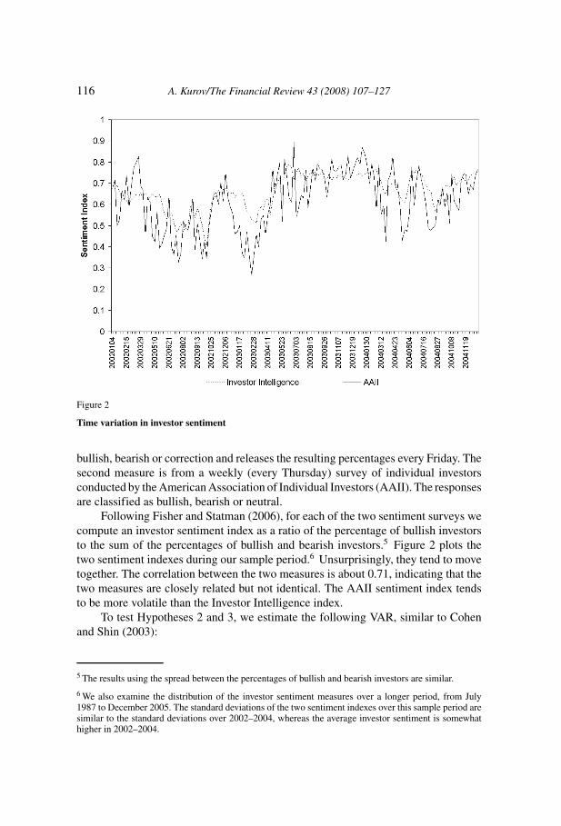
Figure 2

Time variation in investor sentiment

bullish, bearish or correction and releases the resulting percentages every Friday. Thesecond measure is from a weekly (every Thursday) survey of individual investorsconducted by the American Association of Individual Investors (AAII). The responsesare classified as bullish, bearish or neutral.

Following Fisher and Statman (2006), for each of the two sentiment surveys wecompute an investor sentiment index as a ratio of the percentage of bullish investorsto the sum of the percentages of bullish and bearish investors.5 Figure 2 plots thetwo sentiment indexes during our sample period.6 Unsurprisingly, they tend to movetogether. The correlation between the two measures is about 0.71, indicating that thetwo measures are closely related but not identical. The AAII sentiment index tendsto be more volatile than the Investor Intelligence index.

To test Hypotheses 2 and 3, we estimate the following VAR, similar to Cohenand Shin (2003):

5 The results using the spread between the percentages of bullish and bearish investors are similar.

6 We also examine the distribution of the investor sentiment measures over a longer period, from July1987 to December 2005. The standard deviations of the two sentiment indexes over this sample period aresimilar to the standard deviations over 2002–2004, whereas the average investor sentiment is somewhathigher in 2002–2004.


Rt = a1 +3∑

i=0

(b1i + bL

1i DLt−i + bH

1i DHt−i

)Ft−i

+2∑

i=1

(c1i + cL

1i DLt−i + cH

1i DHt−i

)Rt−i + ε1t

Ft = a2 +3∑

i=1

(b2i + bL

2i DLt−i + bH

2i DHt−i

)Ft−i

+2∑

i=0

(c2i + cL

2i DLt−i + cH

2i DHt−i

)Rt−i + ε2t .

(2)

The dummy variable DLt is equal to one on days when the investor sentiment

measure is below its 25th percentile. Similarly, the dummy variable DHt is equal to

one on days when the investor sentiment measure is above its 75th percentile. Thisspecification allows a joint estimation of the VAR in three subsamples: normal days,low-sentiment days and high-sentiment days.

The subsample results are in Table 3. In both E-mini markets and for bothsentiment measures, the effect of recent returns on order flow tends to be significantlygreater in periods of bullish sentiment. Supporting Hypothesis 2, this result showsthat positive feedback trading increases when investors are optimistic. This findingsuggests that sentiment-driven noise trading is likely to increase positive feedbacktrading. The long-run price impact of order flow is significantly smaller on high-sentiment days than on low-sentiment days. Consistent with Hypothesis 3, this resultimplies a negative relation between information content of order flow and investorsentiment.

Our VAR captures serial dependencies in returns and order flows at very shorthorizons. Therefore, it is possible that the price impacts that we interpret as permanentare, at least in part, temporary price pressure effects that are eventually reversed.Under this interpretation, the results suggest that index futures markets tend to bemore liquid in periods of bullish sentiment, with the higher liquidity reducing theprice pressure effects. The subsample results also show that, controlling for feedbacktrading, the persistence of order flow is significantly lower in high-sentiment periods.At the same time, the negative serial correlation of one-minute returns increases inperiods of bullish sentiment.

An alternative way to test Hypotheses 2 and 3 is to estimate the VAR separatelyfor each week and examine time variation in the impulse responses. We use weeklyestimation intervals because our investor sentiment measures are available at weeklyintervals. Figure 3 shows the intensity of feedback trading for each week in the samplefor both E-mini futures markets. There seems to be an increase in positive feedbacktrading in 2003 and 2004 and substantial variation throughout the sample.

We use the following regression model to test Hypothesis 2:

C Ft = α + β1Sentimentt + β2t + β3t2 + β4Volumet + εt . (3)

118 A. Kurov/The Financial Review 43 (2008) 107–127Ta

ble

3

VA

Rre

sult

sin

subs

ampl

es

The

tabl

ere

port

ssu

ms

ofdi

ffer

entc

ombi

natio

nsof

coef

fici

ents

from

the

follo

win

gV

AR

:

Rt=

a 1+

3 ∑ i=0

( b 1i+

bL 1i

DL t−

i+

bH 1i

DH t−

i) Ft−

i+

2 ∑ i=1

( c 1i+

cL 1iD

L t−i+

cH 1iD

H t−i) R

t−i+

ε1t

,

Ft=

a 2+

3 ∑ i=1

( b 2i+

bL 2i

DL t−

i+

bH 2i

DH t−

i) Ft−

i+

2 ∑ i=0

( c 2i+

cL 2iD

L t−i+

cH 2iD

H t−i) R

t−i+

ε2t

,

whe

reD

L tis

adu

mm

yva

riab

leeq

ualt

oon

eon

days

whe

nth

egi

ven

inve

stor

sent

imen

tmea

sure

isbe

low

the

25th

perc

entil

ean

dD

L teq

uals

one

the

give

nin

vest

orse

ntim

entm

easu

reis

abov

eth

e75

thpe

rcen

tile

foro

ursa

mpl

e.T

here

port

edva

lues

are

sum

sof

coef

fici

ents

fort

hedi

ffer

ents

ubsa

mpl

es.F

orex

ampl

e,th

eva

lues

inth

ero

w“N

orm

al”

days

for

the

orde

rfl

owco

effi

cien

tsin

the

retu

rneq

uatio

nar

eca

lcul

ated

as∑ 3 i=

0b 1

i.T

heva

lues

inth

e“L

owSe

ntim

ent”

row

for

the

orde

rfl

owco

effi

cien

tsin

the

retu

rneq

uatio

nar

eca

lcul

ated

as∑ 3 i=

0(b

1i+

DL t−

i),a

ndso

on.T

heva

lues

inth

e“L

owvs

.Nor

mal

”ro

wsh

owad

ditio

nale

ffec

tsin

the

low

-sen

timen

tsu

bsam

ple

and

are

calc

ulat

edas

∑ 3 i=0

(DL t−

i),a

ndso

on.R

etur

nsar

eca

lcul

ated

as10

0tim

esth

elo

gdi

ffer

ence

ofth

epr

ice.

Ord

erfl

ows

are

inth

ousa

nds

ofco

ntra

cts.

Ret

urns

and

orde

rflo

ws

are

aggr

egat

edin

one-

min

ute

inte

rval

s.T

heco

effi

cien

tsof

prim

ary

inte

rest

are

show

nin

bold

.The

sam

ple

peri

odis

from

Janu

ary

1,20

02th

roug

hD

ecem

ber

30,2

004.

Inve

stor

Inte

llige

nce

sent

imen

tind

exA

AII

sent

imen

tind

ex

E-m

iniS

&P

500

E-m

iniN

asda

q-10

0E

-min

iS&

P50

0E

-min

iNas

daq-

100

Rt

equa

tion

Ft

equa

tion

Rt

equa

tion

Ft

equa

tion

Rt

equa

tion

Ft

equa

tion

Rt

equa

tion

Ft

equa

tion

Coe

ffic

ient

son

orde

rfl

ow“N

orm

al”

days

0.05

55∗∗

0.16

79∗∗

0.23

35∗∗

0.10

49∗∗

0.05

78∗∗

0.17

70∗∗

0.23

43∗∗

0.11

07∗∗

Low

sent

imen

t0.

1245

∗∗0.

1538

∗∗0.

4809

∗∗0.

0933

∗∗0.

1065

∗∗0.

1499

∗∗0.

4242

∗∗0.

0968

∗∗H

igh

sent

imen

t0.

0480

∗∗0.

0223

∗∗0.

1919

∗∗0.

0133

∗∗0.

0495

∗∗0.

0847

∗∗0.

2022

∗∗0.

0556

∗∗L

owvs

.nor

mal

0.06

91∗∗

−0.0

141

0.24

74∗∗

−0.0

117

0.04

87∗∗

−0.0

271∗

0.18

99∗∗

−0.0

139

Hig

hvs

.nor

mal

−0.

0075

∗∗−0

.145

6∗∗

−0.

0417

∗∗−0

.091

6∗∗

−0.

0084

∗∗−0

.092

3∗∗

−0.

0321

∗∗−0

.055

1∗∗

(con

tinu

ed)


Tabl

e3

(con

tinu

ed)

Inve

stor

Inte

llige

nce

sent

imen

tind

exA

AII

sent

imen

tind

ex

E-m

iniS

&P

500

E-m

iniN

asda

q-10

0E

-min

iS&

P50

0E

-min

iNas

daq-

100

Rt

equa

tion

Ft

equa

tion

Rt

equa

tion

Ft

equa

tion

Rt

equa

tion

Ft

equa

tion

Rt

equa

tion

Ft

equa

tion

Coe

ffic

ient

son

retu

rns

“Nor

mal

”da

ys−0

.161

0∗∗

14.6

1∗∗

−0.1

309∗

∗3.

55∗∗

−0.1

433∗

∗13

.18∗

∗−0

.120

7∗∗

3.39

∗∗L

owse

ntim

ent

−0.1

400∗

∗6.

87∗∗

−0.1

027∗

∗1.

79∗∗

−0.1

289∗

∗7.

73∗∗

−0.1

004∗

∗1.

94∗∗

Hig

hse

ntim

ent

−0.3

246∗

∗26

.23∗

∗−0

.260

5∗∗

6.28

∗∗−0

.253

3∗∗

21.3

6∗∗

−0.1

983∗

∗5.

09∗∗

Low

vs.n

orm

al0.

0210

−7.

74∗∗

0.02

81∗∗

−1.

76∗∗

0.01

43−

5.46

∗∗0.

0202

−1.

44∗∗

Hig

hvs

.nor

mal

−0.1

635∗

∗11

.61∗

∗−0

.129

6∗∗

2.73

∗∗−0

.110

1∗∗

8.18

∗∗−0

.077

7∗∗

1.71

∗∗

Adj

uste

dR

20.

350.

500.

260.

440.

310.

460.

240.

41D

Wst

atis

tic2.

002.

002.

002.

002.

002.

002.

002.

00

∗ ,∗∗

indi

cate

that

the

null

hypo

thes

isof

aW

ald

test

for

the

sum

ofco

effi

cien

tsbe

ing

equa

lto

zero

isre

ject

edat

5%an

d1%

leve

ls,r

espe

ctiv

ely.


0

10

20

30

40

5020

0201

04

2002

0215

2002

0329

2002

0510

2002

0621

2002

0802

2002

0913

2002

1025

2002

1206

2003

0117

2003

0228

2003

0411

2003

0523

2003

0703

2003

0815

2003

0926

2003

1107

2003

1219

2004

0130

2004

0312

2004

0423

2004

0604

2004

0716

2004

0827

2004

1008

2004

1119

net

bu

ys/s

ells

('0

00 c

on

trac

ts)

E-mini S&P 500 futures E-mini Nasdaq-100 futures

Figure 3

Feedback trading over time

The graph shows time variation in the cumulative effect of a 1% return shock on the order flow.

CFt is the cumulative impulse response of the order flow (in thousands of con-tracts) after a unit return shock. The impulse responses are calculated separately foreach week t. Sentimentt is the value of the investor sentiment index, and Volumet is thetrading volume in the particular E-mini futures contract during week t (in millions ofcontracts). The trading volume is included as a regressor to control for a possible in-crease in the feedback trading explained by the overall increase in the trading activityin the E-mini markets. The model also includes a quadratic trend. A nonlinear trend infeedback trading is apparent in Figure 3. The regression in Equation (3) is estimatedusing OLS with the Newey and West (1987) heteroskedasticity and autocorrelationconsistent covariance matrix.

The results in Table 4 appear to corroborate the subsample VAR results, showingthat positive feedback trading increases during periods of bullish sentiment, control-ling for time trend and changes in overall trading activity. The coefficient estimatesof sentiment are positive and statistically significant in all cases. These coefficientestimates are smaller when the AAII sentiment index is used, possibly due to thehigher overall variability in this sentiment measure.7 The coefficients of the trend

7 The difference between the coefficients of the two investor sentiment measures becomes much smallerif we standardize the two measures by dividing them by their sample standard deviations.


Table 4

Estimates of the effect of sentiment on feedback trading

The estimated coefficients are for the regression:

C Ft = α + β1 Sentimentt + β2t + β3t2 + β4 Volumet + εt .

CFt is the cumulative impulse response of the order flow (in thousands of contracts) after a unit return shock.The impulse responses are calculated separately for each week t, as discussed in Section 4.2. Sentimentt isa measure of investor sentiment during week t, and Volumet is the trading volume in the particular E-minifutures contract (in millions of contracts) during week t. The sample period is from January 1, 2002 throughDecember 30, 2004. The sample contains 156 weekly observations. The regression is estimated using OLSwith the Newey and West (1987) heteroskedasticity and autocorrelation consistent covariance matrix. Thecoefficients of primary interest are shown in bold. Absolute values of t-statistics are in parentheses.


Panel A: With Investor Intelligence sentiment index

Intercept −9.63 (2.77)∗∗∗ −1.79 (2.96)∗∗∗Sentiment 21.97 (4.85)∗∗∗ 4.66 (6.17)∗∗∗

t 20.26 (3.75)∗∗∗ 2.58 (2.34)∗∗t2 17.34 (2.72)∗∗∗ 5.93 (4.28)∗∗∗Trading volume −0.10 (0.17) 0.20 (0.44)Adjusted R2 0.91 0.92

Panel B: With AAII sentiment index

Intercept −3.21 (1.26) −0.27 (0.48)Sentiment 11.76 (4.53)∗∗∗ 2.17 (5.09)∗∗∗

t 23.92 (5.16)∗∗∗ 3.33 (3.05)∗∗∗t2 15.35 (2.60)∗∗∗ 5.57 (4.12)∗∗Trading volume −0.20 (0.36) 0.17 (0.38)Adjusted R2 0.92 0.92

∗, ∗∗, and ∗∗∗ indicate statistical significance at 10%, 5%, and 1% levels, respectively.

terms are positive and statistically significant, indicating an overall increase in positivefeedback trading over our sample period.

To examine the relation between informativeness of order flow and investorsentiment, we estimate the regression:

CRt = α + β1 Sentimentt + β2t + β3t2 + β4 Volumet + εt , (4)

where CRt is the cumulative impulse response of returns after a 1,000-contract shockfrom the order flow. These cumulative impulse responses measure the informationcontent of trades. Similar to Equation (3), the regression also includes a quadratictime trend and the trading volume in the particular E-mini market.

The results are in Table 5. The coefficient β2 is negative and statistically signif-icant in all cases, suggesting an overall decline in the information content of orderflow across the sample period. This decline could be related to increasing liquidityin the E-mini markets. Consistent with Hypothesis 3, the coefficient of the investor


Table 5

Estimates of the effect of sentiment on informativeness of order flow

The estimated coefficients are for the following regression:

CRt = α + β1 Sentimentt + β2t + β3t2 + β4 Volumet + εt .

CRt is the cumulative impulse response of returns after a 1,000-contract shock from the order flow. Theimpulse responses are calculated separately for each week t, as discussed in Section 4.2. Sentimentt is ameasure of investor sentiment during week t, and Volumet is the trading volume in the particular E-minifutures contract (in millions of contracts) during week t. The sample period is from January 1, 2002 throughDecember 30, 2004. The sample contains 156 weekly observations. The regression is estimated using OLSwith the Newey and West (1987) heteroskedasticity and autocorrelation consistent covariance matrix. Thecoefficients of primary interest are shown in bold. Absolute values of t-statistics are in parentheses.



Intercept 0.40 (9.47)∗∗∗ 1.39 (8.83)∗∗∗Sentiment −0.27 (3.82)∗∗∗ −0.90 (3.55)∗∗∗

t −0.44 (5.90)∗∗∗ −1.37 (6.85)∗∗∗t2 0.25 (4.32)∗∗∗ 0.72 (4.52)∗∗∗Trading volume 0.01 (0.90) 0.02 (0.70)Adjusted R2 0.81 0.88


Intercept 0.27 (10.74)∗∗∗ 1.06 (12.50)∗∗∗Sentiment −0.07 (2.18)∗∗ −0.36 (3.07)∗∗∗

t −0.53 (6.53)∗∗∗ −1.53 (6.84)∗∗∗t2 0.30 (4.99)∗∗∗ 0.79 (4.53)∗∗∗Trading volume 0.01 (1.43) 0.03 (0.85)Adjusted R2 0.78 0.85

∗∗∗, ∗∗, ∗ indicate statistical significance at the 0.01, 0.05 and 0.10 level, respectively.

sentiment index is negative for both markets and both sentiment measures, whichimplies that order flow tends to be less informative in bullish periods.

4.3. Effect of investor sentiment on transitory volatility

To test Hypothesis 4, relating to the relation between investor sentiment andtransitory volatility, we estimate transitory volatility using the variance decompositionapproach of Hasbrouck (1993). The underlying model of the security price is:

pt = mt + st , (5)

mt = mt−1 + wt . (6)

The random walk component mt is the “efficient price” that represents a condi-tional expectation of the security’s terminal value. The pricing error st represents the


deviation from the efficient price. It is driven by market frictions and noise trading.The variance of the pricing error is a natural measure of transitory volatility.

We estimate the pricing error variance using Hasbrouck’s (1993) model. Specif-ically, we estimate the following VAR with four Equations:[

rt

xt

]=

k∑i=1

Ai

[rt−i

xt−i

]+

[vrt

vxt

], (7)

where rt are returns based on trade prices and xt is a vector of three variables: (1) avariable representing signed trades (equal to one for buys and minus one for sells), (2)signed trade volume and (3) signed square root of the trade volume. Ai are coefficientmatrices and vt are serially uncorrelated innovations with a covariance matrix cov(v).In contrast to the VAR model used to examine feedback trading, this model includesno contemporaneous returns or signed volumes and uses no time aggregation, i.e.,the subscript t indexes transactions. The trade-by-trade returns are computed withoutcorrection for the bid-ask bounce. We estimate the VAR separately in each weeklyinterval in our sample using 10 lags of all variables in the model.8

Hasbrouck (1993) shows that the pricing error in Equation (5) can be estimatedas:

st =∞∑j=0

α j vr,t− j +∞∑j=0

β1 j vx1,t− j +∞∑j=0

β2 j vx2,t− j +∞∑j=0

β3 j vx3,t− j . (8)

Intuitively, the pricing error is driven by temporary impacts of innovations inreturns and trades, as well as by lagged adjustment to information. The α and β

coefficients in Equation (8) are obtained from a vector moving average (VMA) rep-resentation of the VAR in Equation (7). We obtain the VMA coefficients from impulseresponses and estimate the variance of the pricing error for each weekly interval as9 :

σ 2s =

∞∑j=0

[ α j β j ]cov(v)

[α j

β ′j

]. (9)

To examine the relation between transitory volatility and investor sentiment, weconsider the following regression:

σ 2st = α + β1Sentimentt + β2t + β3t2 + β4Volumet + β5σ

2t + εt , (10)

where σ 2t is the variance of daily returns on the index underlying the particular E-

mini contract, estimated with a GARCH(1,1) model and sampled on the days whenInvestor Intelligence releases its sentiment measures. The sentiment in this model canbe viewed as a proxy for noise trading activity. Investor sentiment may be correlatedwith transitory volatility because it is correlated with the overall return volatility,

8 The regression results discussed below are not affected qualitatively by the number of lags in the VAR.

9 Hasbrouck (1993) shows that this expression represents the lower bound of σ 2s . The actual value of the

pricing error variance may exceed the lower bound due to factors uncorrelated with lagged returns andsigned trades.


Table 6

Estimates of the effect of sentiment on transitory volatility

The estimated coefficients are for the following regression:

σ 2st = α + β1Sentimentt + β2t + β3t2 + β4Volumet + β5σ

2t + εt .

σ 2st is the variance of the pricing error (transitory volatility) estimated separately for each week t, as

discussed in Section 4.3. Sentimentt is a measure of investor sentiment during week t, Volumet is thetrading volume in the particular E-mini futures contract (in millions of contracts) during week t, and σ 2

tis the variance of daily returns on the index underlying the particular E-mini contract, estimated with aGARCH(1,1) model. The sample period is from January 1, 2002 through December 30, 2004. The samplecontains 156 weekly observations. The regression is estimated using OLS with the Newey and West (1987)heteroskedasticity and autocorrelation consistent covariance matrix. All coefficients are multiplied by 105.The coefficients of primary interest are shown in bold. Absolute values of t-statistics are in parentheses.




t 5.64 (4.25)∗∗∗ 12.32 (6.70)∗∗∗t2 −6.17 (5.56)∗∗∗ −12.20 (7.24)∗∗∗Trading volume 0.28 (1.86)∗ 0.11 (0.32)Daily volatility 0.47 (3.67)∗∗∗ 0.89 (8.48)∗∗∗Adjusted R2 0.79 0.90



t 3.99 (3.06)∗∗∗ 10.86 (5.22)∗∗∗t2 −4.91 (4.84)∗∗∗ −10.81 (5.76)∗∗∗Trading volume 0.33 (1.92)∗ 0.31 (0.78)Daily volatility 0.66 (5.62)∗∗∗ 1.14 (10.70)∗∗∗Adjusted R2 0.77 0.87

∗∗∗, ∗∗, ∗ indicate statistical significance at the 0.01, 0.05 and 0.01 level, respectively.

and the return volatility is correlated with transitory volatility. We include the returnvolatility in the regression to test whether sentiment-driven trading affects the varianceof the pricing error for a given return volatility.

The regression estimates are in Table 6. As expected, the results show a strongpositive relation between the variance of the pricing error and return volatility. Re-jecting Hypothesis 4, the coefficient of sentiment is also statistically significant andnegative for both E-mini markets and both sentiment measures, suggesting that indexfutures prices tend to follow the underlying efficient price more closely in bullishperiods, consistent with increased liquidity in bullish states (e.g., Baker and Stein,2004).

The lower variance of the pricing error in periods of high investor senti-ment is not inconsistent with the reduced information content of order flow in the


previous subsection. Increased liquidity trading in high-sentiment states can simul-taneously lead to lower average information content of trades and lower transitoryvolatility.

Hasbrouck (1993, p. 196) notes that empirical microstructure models that onlyaccount for very high-frequency serial dependencies, such as the VAR model used toestimate the pricing error variance, tend to impound low-frequency transitory compo-nents of prices into the “efficient price.” Therefore, it is possible that transitory volatil-ity observed at intraday frequencies declines in periods of high investor sentiment,whereas, as Brown and Cliff (2005) show, long-horizon pricing errors increase.10

4.4. Robustness checks

A potential concern in regressions using levels of economic time series is thespurious regression problem discussed by Granger and Newbold (1974). When two in-dependent nonstationary variables are regressed on each other, the results may suggesta significant relation between the two variables. We use Augmented Dickey-Fullerand Phillips-Perron unit root tests to test the stationarity of the investor sentimentmeasures and the dependent variables in our regressions. An intercept and a lineartrend are included in the test equation. In all cases, with the exception of transitoryvolatility in the E-mini Nasdaq-100 market, the null of the unit root is rejected by oneor both of the tests. When the unit root tests are repeated for residuals from regressionsof the two sentiment measures and the three dependent variables on a quadratic trend,the null of the unit root is rejected by both tests at the 1% level in all cases. Theseresults indicate that our variables are trend-stationary.

In a spurious regression, the error term is nonstationary (e.g., Stock and Watson,1988, p. 166). We examine residual autocorrelations and test for the unit root inthe residuals for all our regressions. The first-order serial correlation of regressionresiduals never exceeds 0.7 and the null hypothesis of unit root in the residuals isrejected in all cases, suggesting that the results are not affected by the spuriousregression problem. Furthermore, the results of the regression tests of Hypotheses 2and 3 are supported by the subsample VAR results reported in Table 3.

To explicitly account for serial correlation in the regression residuals, we alsoestimate the regressions in Equations (3), (4), and (10) using maximum likelihoodwith AR(1) residuals. The results are qualitatively similar to the OLS results. SinceOLS estimation could be sensitive to the presence of outliers, we also estimate theregressions using the weighted least squares procedure introduced by Yohai (1987).This procedure maintains robustness in the presence of a large number of outliers.The results again are qualitatively similar to the OLS results. Finally, we experimentwith two additional proxies for investor sentiment: the UBS/Gallup Index of InvestorOptimism and the forward P/E ratio of the S&P 500 index .11 Both measures are

10 Brown and Cliff (2005) estimate pricing errors for the aggregate stock market using monthly data.

11 Fisher and Statman (2006) use the P/E ratio of the S&P 500 index as an indirect measure of sentiment.


available monthly. The regression results are qualitatively similar. The robustnesschecks are not reported in detail but are available from the author.

5. Conclusion

This paper examines how the order flow of traders in index futures markets isaffected by recent price changes. We show that index futures traders use positivefeedback trading strategies, i.e., they buy index futures contracts after price increasesand sell after price declines. Such positive feedback trading has become more prevalentin index futures markets in recent years. We also find a positive relation betweenintensity of the positive feedback trading and investor sentiment. This result suggeststhat positive feedback trading consists, at least in part, of sentiment-driven noisetrading.

Consistent with the noise trading hypothesis, we find that order flow containsless information in periods of bullish sentiment. Finally, we find a strong negativerelation between the variance of the pricing error estimated at intraday frequenciesand investor sentiment measures. This finding implies that sentiment-driven tradingincreases market liquidity, helping to stabilize temporary price fluctuations. Overall,this paper provides new evidence on the link between investor attitudes, tradingbehavior and price efficiency at the microstructure level.

References

Antoniou, A., G. Koutmos, and A. Pericli, 2005. Index futures and positive feedback trading: Evidencefrom major stock exchanges, Journal of Empirical Finance 12, 219–238.

Baker, M. and J. Stein, 2004. Market liquidity as a sentiment indicator, Journal of Financial Markets 7,271–299.

Baker, M. and J. Wurgler, 2006. Investor sentiment and the cross-section of stock returns, Journal ofFinance 61, 1645–1680.

Bange, M.M., 2000. Do the portfolios of small investors reflect positive feedback trading? Journal ofFinancial and Quantitative Analysis 35, 239–255.

Brandt, M. and K. Kavajecz, 2004. Price discovery in the U.S. Treasury market: The impact of orderflowand liquidity on the yield curve, Journal of Finance 59, 2623–2654.

Brown, G.W. and M.T. Cliff, 2004. Investor sentiment and the near-term stock market, Journal of EmpiricalFinance 11, 1–27.

Brown, G.W. and M.T. Cliff, 2005. Investor sentiment and asset valuation, Journal of Business 78, 405–440.Cohen, B.H. and H.S. Shin, 2003. Positive feedback trading under stress: Evidence from the U.S. Treasury

securities market. Working paper, London School of Economics.Danielsson, J. and R. Love, 2006. Feedback trading, International Journal of Finance and Economics 11,

35–53.De Long, J.B., A. Shleifer, L.H. Summers, and R.J. Waldmann, 1990. Positive feedback investment strate-

gies and destabilizing rational speculation, Journal of Finance 45, 379–395.Evans, M.D.D. and R.K. Lyons, 2002. Order flow and exchange rate dynamics, Journal of Political

Economy 110, 170–180.Finucane, T.J., 2000. A direct test of methods of inferring trade direction from intraday data, Journal of

Financial and Quantitative Analysis 35, 553–576.Fisher, K.L. and M. Statman, 2006. Market timing in regressions and reality, Journal of Financial Research

29, 293–304.


French, K. and R. Roll, 1986. Stock return variances: The arrival of information and the reaction of traders,Journal of Financial Economics 17, 5–26.

Glosten, L. and P. Milgrom, 1985. Bid, ask, and transaction prices in a specialist market with heteroge-neously informed traders, Journal of Financial Economics 13, 71–100.

Granger, C.W.J. and P. Newbold, 1974. Spurious regressions in econometrics, Journal of Econometrics 2,111–120.

Hasbrouck, J., 1991. Measuring the information content of stock trades, Journal of Finance 46, 179–207.Hasbrouck, J., 1993. Assessing the quality of a security market: A new approach to transaction-cost

measurement Review of Financial Studies 6, 191–212.Hasbrouck, J., 2003. Intraday price formation in US equity index markets, Journal of Finance 58, 2375–

2399.Kandel, E. and N.D. Pearson, 1995. Differential interpretation of public signals and trade in speculative

markets, Journal of Political Economy 103, 831–872.Kyle, A.S., 1985. Continuous auctions and insider trading, Econometrica 53, 1315–1335.Manaster, S. and S.C. Mann, 1996. Life in the pits: Competitive market making and inventory control,

Review of Financial Studies 9, 953–975.Newey, W. and K. West, 1987. A simple positive semi-definite, heteroskedasticity and autocorrelation

consistent covariance matrix, Econometrica 55, 703–708.Nofsinger, J.R. and R.W. Sias, 1999. Herding and feedback trading by institutional investors, Journal of

Finance 54, 2263–2295.Sentana, E. and S. Wadhwani, 1992. Feedback traders and stock return autocorrelations: Evidence from a

century of daily data, Economic Journal 102, 415–425.Shu, T., 2007. Does positive-feedback trading by institutions contribute to stock return momentum? Working

paper, University of Texas at Austin.Sias, R.W., 2007. Reconcilable differences: Momentum trading by institutions, The Financial Review 42,

1–22.Stock, J.H. and M.W. Watson, 1988. Variable trends in economic time series, Journal of Economic Per-

spectives 2, 147–174.Subrahmanyam, A., 1991. A theory of trading in stock index futures, Review of Financial Studies 4, 17–51.Yan, X. and S. Ferris, 2004. The relation between online trading and stock market behavior. Working

paper, University of Missouri–Columbia.Yohai, V.J., 1987. High breakdown-point and high efficiency robust estimates for regression, Annals of

Statistics 15, 642–656.

investor sentiment, trading behavior and informational ... · the financial review 43 (2008)...

Documents