trade policy preferences and cross-regional differences: … · *this study is conducted as a part...
TRANSCRIPT

DPRIETI Discussion Paper Series 15-E-003
Trade Policy Preferences and Cross-Regional Differences:Evidence from individual-level data of Japan
ITO BanriHarvard University / Senshu University
MUKUNOKI HiroshiGakushuin University
TOMIURA EiichiRIETI
WAKASUGI RyuheiRIETI
The Research Institute of Economy, Trade and Industryhttp://www.rieti.go.jp/en/
1
RIETI Discussion Paper Series 15-E-003
January 2015
Trade Policy Preferences and Cross-Regional Differences: Evidence from individual-level data of Japan*
ITO Banri (Harvard University, Senshu University)
MUKUNOKI Hiroshi (Gakushuin University)
TOMIURA Eiichi (RIETI, Yokohama National University)
WAKASUGI Ryuhei (RIETI, Gakushuin University)
Abstract
This study examines the determinants of individuals’ preferences for trade policies, using micro data of 10,000 individuals selected from Japan’s general population. In particular, we focus on the role of regional factors that influence trade policy preferences, considering the fact that there is a significant difference in preferences among regions. The results of the binary choice model reveal that local characteristics affect people’s views on trade policy even after controlling for labor market and non-economic attributes. Specifically, people residing in a region with a high share of agricultural workers are likely to support import restrictions even if they do not engage in agriculture, which is the most protected sector in Japan. Moreover, there is a strong correlation between the probability of supporting the protectionist trade policy and the share of local agricultural workers for people not considering migration, suggesting that inter-regional immobility of workers affects their trade policy preferences.
Keywords: Trade policy, Policy preferences, Agriculture, Regional economy
JEL Classifications: F13,Q17,R10
RIETI Discussion Papers Series aims at widely disseminating research results in the form of professional
papers, thereby stimulating lively discussion. The views expressed in the papers are solely those of the
author(s), and neither represent those of the organization to which the author(s) belong(s) nor the Research
Institute of Economy, Trade and Industry.
* This study is conducted as a part of the Project “Empirical Analysis of Trade Policy Preferences at the Individual Level in Japan” undertaken at the Research Institute of Economy, Trade and Industry (RIETI). This study employs data derived from a survey conducted by RIETI. The authors are grateful to Masahisa Fujita, Masahiro Kawai, Masayuki Morikawa, Yasuyuki Todo, and other seminar participants at RIETI. We gratefully acknowledge the useful comments of Elhanan Helpman. This study was conducted while Ito was a Visiting Scholar in the Weatherhead Center at Harvard University. He acknowledges Harvard University for their support and the program on U.S.–Japan relations for its hospitality.
1. Introduction Building a consensus for advancing trade liberalization among people is difficult as
experienced by many countries. People’s views on trade policies are different because trade
liberalization does not equally benefit all people. For instance, in Japan, although public opinion
polls indicate that the majority of people are in favor of free trade, statistics reveal that 20% to 30%
of the population, mainly in local areas, objects free trade policies. Currently, it is likely that regional
factors are one of the important determinants of trade policy preferences in Japan as dissenting
opinions are heavily concentrated in rural areas. The common perception is that people engaged in
the agricultural sector oppose free trade because of its long history of government protectionism.1
However, it is not only those in the agricultural industry that object, considering that the agricultural
industry comprises only 1% of the total GDP and the agricultural workforce is only 3% of the total.2
Although people are not agricultural workers, it is believed that they object to further trade
liberalization for the fear of being indirectly affected by a declining regional economy. If this is the
case, in addition to individuals’ labor market attributes, such as education and industry affiliation,
which have been examined by previous studies, regional characteristics are likely to be correlated
with people’s preferences for trade policy. Regardless of whether people work in the agricultural
sector and whether they are currently employed or retired, people might be more likely to support
protectionism if they reside in a region with a high share of agricultural workers and a high
unemployment rate. The significant effect of regional factors could correspond to the inter-regional
immobility of workers, which has not been explicitly analyzed in existing studies. This study focuses
on the role of these local characteristics in determining trade policy preferences.
Previous studies at the individual level have focused on the role of labor market attributes
in determining trade policy preferences, based on the predictions of trade theory (Scheve and
Slaughter, 2001; Beaulieu, 2002a; Mayda and Rodrik, 2005; Blonigen, 2011).3 They examined
whether individuals’ skill endowments, such as education or industry affiliation, could explain their
trade policy preferences.4Although they found a correlation between individuals’ labor market
attributes and trade policy preferences, other than labor market attributes, it is shown that some other
1 According to the World Tariff Profiles 2014, Japan’s average most favored nation (MFN) applied tariff rate on agricultural products is 19%, which is relatively higher than that of the European Union (13.2%) or the United States (5.3%). 2 Despite the declining share in population, agricultural protectionism is observed in many developed countries, as referenced, for example, in the study by Davis (2004). 3 Earlier studies on the origins of protectionist trade policy based on political economy have focused on the role of lobbying and campaign contributions of specific interest groups in maintaining protectionist trade policies (Magee, 1980; Grossman and Helpman, 1994; 2005). Some empirical evidence suggests a positive correlation between protectionism and lobbying (Goldberg and Maggi, 1999; McCalman, 2004; Evans, 2009; Fredriksson, 2010). 4 Similarly, Kaempfer and Marks (1993), Baldwin and Magee (2000), and Beaulieu (2002b)
examined the determinants of votes for trade liberalization bills by Members of Congress, introducing both endowment and industry variables in their representative districts.
2
variables, which have not been considered by conventional trade theory, had a strong correlation
with trade policy preferences. For example, Scheve and Slaughter (2001) and Blonigen (2011)
reported significant asset effects on trade policy preferences. They hypothesized that people who
reside in a region wherein comparatively disadvantaged industries are dominant are likely to face
negative demand shocks in the housing market after trade liberalization. Therefore, it is foreseen that
housing prices will decline in these areas. Their results indicate that homeowners tend to support
trade protection more as the level of concentration of comparatively disadvantage sectors increases
in their regions. Moreover, this result suggests that not only individual characteristics but also
regional factors influence trade policy preferences. However, the literature on the origins of
protectionism has not focused on the direct relationship between regional characteristics and
individuals’ trade policy preferences till today.
This study empirically examines the association between regional factors and people’s
trade policy preferences. In addition, this study clarifies the factors leading to protectionism support,
using micro data of 10,816 individuals selected from the general population all over Japan. To the
best of our knowledge, the size of our sample is the largest compared to that of previous studies.5
We use the binary choice model to determine the probability of supporting import restrictions. The
main results of this study are threefold. First, it is confirmed that trade policy preferences are
heterogeneous depending on the region even after controlling for labor market and non-economic
attributes. Individuals residing in a region with a high share of agricultural workers and
unemployment rate tend to support a protectionist trade policy even if they do not engage in that
sector. Second, for people who are considering residing in the region, the probability of supporting a
protectionist trade policy increases as the proportion of agricultural workers increases. However,
there is no correlation between the probability of supporting a protectionist trade policy and the
regional agricultural workers ratio for people considering migration. Third, people who do not own a
house in areas with a low unemployment rate are likely to support a protectionist trade policy;
however, if the unemployment rate increases, the probability of supporting protectionism decreases.
In contrast, people who own houses exhibit a higher probability of supporting a protectionist trade
policy as the unemployment rate rises. These results suggest that inter-regional worker’s immobility
affects individuals’ trade policy preferences. Our results are robust to a multi-level mixed logistic
model, which enables us to control for unobserved region-specific factors and examine the
difference in the influence of covariates on trade policy preferences, depending on the regions.
The remainder of this study is organized as follows. Section 2 presents an empirical
framework to explain the probability of choosing trade policy preferences and describes data on
5 The exception is a cross-country analysis by Mayda and Rodrik (2005) that used 28,456 observations distributed over 23 countries. As a single country study, 5,224 observations in Blonigen (2011) was the largest sample till date.
3
trade policy preferences. Section 3 presents the results of the logistic regression. Section 4 presents
the results of the multi-level model. Section 5 concludes the study.
2. Empirical framework and data 2.1. Binary choice model
We empirically examine whether an individual supports a protectionist or free trade policy
under the binary choice model. PijU denotes the utility when an individual i who lives in a region j
faces a protectionist trade policy. FijU denotes the utility when an individual faces a free trade
policy. Individuals are expected to support a protectionist trade policy when the utility from the
protectionist trade policy is greater than that from the free trade policy, namely, Fij
Pij UU > . We
consider the difference in the utility between the two as a latent variable *ijy , which is linearly
related with covariates as below:
ijijij ey += βX* , (1)
where ijX is a set of firm-specific regressors, and β is a vector of coefficients. The latent variable *ijy is defined as an observable binary variable that equals 1 if individual i located in region j
supports a protectionist trade policy, and 0 otherwise. ije is the error term distributed as a logistic
function:
≤
>=
0 tradefree:0
0 ist protection:1*
*
ij
ijij yif
yify
The probability of choosing a protectionist trade policy ( 1=ijy ) is expressed as the following:
, (2)
where F denotes the cumulative distribution function of the logistic distribution. The probability of
supporting a free trade policy is written as ( ){ }βX ijijp exp111 +=− . Therefore, the odds ratio of
both probabilities is formed as the following equation:
( ) ( ) ( )( ){ }βXβX
βXij
ijijijij Fyp
exp1exp
1Pr+
====
4
βX ijij
ij
pp
=
−1ln . (3)
In the estimation results, we interpret the results by odds ratio after transforming the
estimated coefficients obtained from the maximum likelihood estimation. Therefore, an odds ratio
beyond unity implies a positive correlation between the probability of supporting a protectionist
trade policy and the covariate, whereas an odds ratio less than unity indicates that it is positively
related with the probability of supporting a free trade policy.
2.2. Trade policy preferences and regional attributes
This study employs micro data on trade policy preferences retrieved from the
“Questionnaire Survey about Japanese Economy and International Trade with Foreign Countries,”
undertaken by the Research Institute of Economy, Trade and Industry (RIETI) in October 2011.6
The survey was conducted with randomly selected people aged 20 to 79 years so that the proportions
of ten regions and twelve age groups approximated those in the recent national population census.
The number of respondents is 10,816 individuals located throughout Japan, which represents
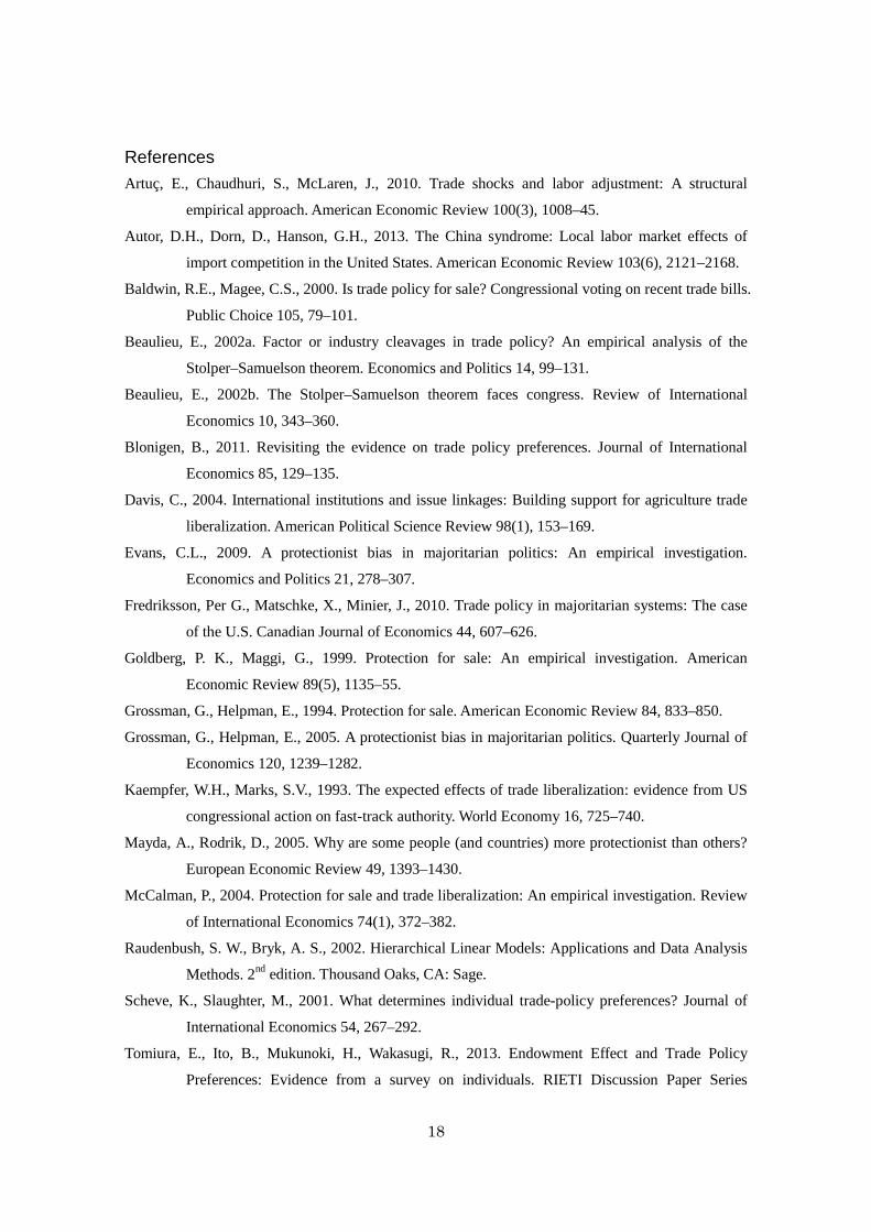
approximately one out of ten thousand of Japan’s total population.7 Regarding people’s views on trade policy, we asked the following question in the survey:8 Answer what you think about the following opinion: “We should further liberalize imports to make wider varieties of goods available at lower prices.” The responses for the five choices presented include the following:
“strongly agree” (8.9%); “somewhat agree” (42.5%); “somewhat disagree” (26.9%); “strongly
disagree” (4.6%); and “cannot choose or unsure” (17.1%). That is, if we aggregate responses that
strongly or somewhat agree with the opinion that imports should be further liberalized as supporters
of free trade, 51% are agreeable, whereas an aggregate of those who somewhat or strongly disagree
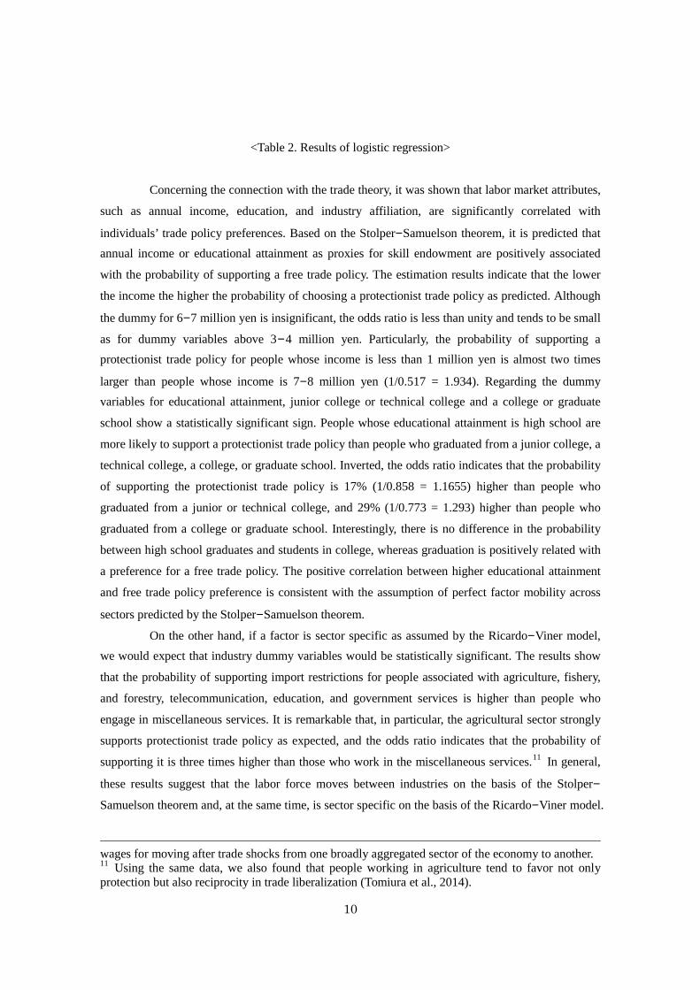
comprise 32%. To overview the differences in trade policy preferences across regions, response
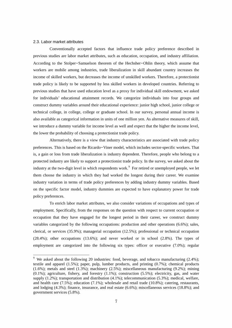
distributions over 10 areas to the import liberalization question are illustrated in Figure 1. A
difference is generally observed among metropolitan areas, such as Keihin (including Tokyo),
Keihanshin (including Osaka), and rural areas, and the ratio of people who object to a free trade
6 Specifically, the survey was conducted by a commercial research company Intage under contract with RIETI for our research project. 7 The response rate of this survey was 31.1%. 97% of the responses were via internet, and the same questionnaire was printed and posted to people aged over 60 years to reach elderly people without internet access. 8 Survey questions from this survey and basic statistics on individual characteristics are available in the appendix of Tomiura et al. (2013).
5

policy, or reply “cannot choose or unsure” is relatively high in Hokkaido, Tohoku, and Kyushu
where agriculture is relatively prosperous.
<Figure1. Response distribution of trade policy preferences by area>
From these five responses, we construct a binary variable that takes a value of 1 if people
choose “somewhat disagree,” “strongly disagree,” or “cannot choose or unsure,” and 0 otherwise,
considering these individuals as protectionists since they are not active supporters for trade
liberalization and are likely to choose inaction. In addition, we verify the sensitivity of results when
the response of “cannot choose or unsure” is excluded.
Regional factors are the key explanatory variables in this study. We employ the ratio of
agriculture workforce at the city and town levels as a proxy for weight of comparatively
disadvantaged industries on the basis of the view that indirect negative effects from structural
changes due to trade liberalization are significant in an area with a high concentration of
comparatively disadvantaged industries. Since people who reside in such areas are expected to
support a protectionist trade policy, it is anticipated that the ratio of agricultural workforce is
positively correlated with the probability of choosing a protectionist trade policy. The data are
retrieved from the national census of 2010. Moreover, we add the unemployment rate at the city
level to consider the structural differences in economic situation among regional economies.
If inter-regional movement is difficult for people residing in areas where these local
characteristic values are high, it is predicted that the probability of supporting a protectionist trade
policy increases. In contrast, people who have a high inclination of migrating are able to avoid
structural adjustments after trade liberalization and may seek new employment opportunities in other
areas. In the survey, we set the question item: “Do you have a plan to move or want to move in
future?” to control for differences in trade policy preferences between those inclined and those not
inclined to migrate. The responses to the four choices presented include the following: “I’m going to
do or I want to do” (11.3%); “I want to do if there is an opportunity” (24.2%); “I do not want to do
if it is possible” (18.8%); and “I do not want to do” (45.8%). From these results, we construct a
dummy variable that takes a value of 1 for people who show a positive attitude toward moving and 0
otherwise. The sign of the mobility dummy variable is expected to be negative. Since it is anticipated
that the impacts of regional characteristics are different between people considering migration and
those who are not, we also examine whether interaction terms of the mobility dummy and regional
variables are significant. It is predicted that the effects of local characteristics on the probability of
supporting import restrictions is small or insignificant for people considering migration.
6
2.3. Labor market attributes
Conventionally accepted factors that influence trade policy preference described in
previous studies are labor market attributes, such as education, occupation, and industry affiliation.
According to the Stolper–Samuelson theorem of the Hechsher–Ohlin theory, which assume that workers are mobile among industries, trade liberalization in skill abundant country increases the
income of skilled workers, but decreases the income of unskilled workers. Therefore, a protectionist
trade policy is likely to be supported by less skilled workers in developed countries. Referring to
previous studies that have used education level as a proxy for individual skill endowment, we asked
for individuals’ educational attainment records. We categorize individuals into four groups and
construct dummy variables around their educational experience: junior high school, junior college or
technical college, in college, college or graduate school. In our survey, personal annual income is
also available as categorical information in units of one million yen. As alternative measures of skill,
we introduce a dummy variable for income level as well and expect that the higher the income level,
the lower the probability of choosing a protectionist trade policy.
Alternatively, there is a view that industry characteristics are associated with trade policy
preferences. This is based on the Ricardo–Viner model, which includes sector-specific workers. That is, a gain or loss from trade liberalization is industry dependent. Therefore, people who belong to a
protected industry are likely to support a protectionist trade policy. In the survey, we asked about the
industry at the two-digit level in which respondents work.9 For retired or unemployed people, we let
them choose the industry in which they had worked the longest during their career. We examine
industry variation in terms of trade policy preferences by adding industry dummy variables. Based
on the specific factor model, industry dummies are expected to have explanatory power for trade
policy preferences.
To enrich labor market attributes, we also consider variations of occupations and types of
employment. Specifically, from the responses on the question with respect to current occupation or
occupation that they have engaged for the longest period in their career, we construct dummy
variables categorized by the following occupations: production and other operations (6.6%); sales,
clerical, or services (35.9%); managerial occupation (12.5%); professional or technical occupation
(28.4%); other occupations (13.6%); and never worked or in school (2.8%). The types of
employment are categorized into the following six types: officer or executive (7.0%); regular
9 We asked about the following 20 industries: food, beverage, and tobacco manufacturing (2.4%); textile and apparel (1.5%); paper, pulp, lumber products, and printing (0.7%); chemical products (1.6%); metals and steel (1.3%); machinery (2.5%); miscellaneous manufacturing (9.2%); mining (0.1%); agriculture, fishery, and forestry (1.1%); construction (5.5%); electricity, gas, and water supply (1.2%); transportation and distribution (4.1%); telecommunication (5.3%); medical, welfare, and health care (7.5%); education (7.1%); wholesale and retail trade (10.8%); catering, restaurants, and lodging (4.3%); finance, insurance, and real estate (6.6%); miscellaneous services (18.8%); and government services (5.8%).
7
employee or public servant (44.9%); non-regular employee (29.4%); self-employment or profession
(14.8%); and in school or no work experience (3.9%).
To control for current employment status, we add a dummy variable that takes a value of 1
if people are employed (61%). In addition, variations of the preferences among individuals
according to inclination toward job change are also considered by a dummy that takes a value of 1
for a positive response to the question “Do you have a plan to change your job or want to change in
future?” People who show an inclination toward job change are 32.3% of the sample and are
expected to have a higher probability of supporting a free trade policy than those who do not.
2.4. Non-economic attributes
Previous studies found that people’s non-economic characteristics are strongly related to
their trade policy preferences. Our model includes basic non-economic attributes, such as age,
gender (female: 48.5%) and family status (having a child: 63.7%). In Japan, it is thought that people
are concerned about food safety issues of imported food. Considering that this concern is likely to
lead them to choose protectionism, we asked a question in the survey: “When you usually purchase
drink and food, do you check an additive and the place of origin?” and introduce a dummy variable
that takes the value of 1 for positive responses (68.9%). As examined by Scheves and Slaugter
(2001) and Blonigen (2011), we also add a dummy variable for people who own a house or an
apartment (72.6%) to examine asset effects of home ownership on trade policy preferences. Policy
preferences may vary depending on ideological differences. In the survey, we set the question item
“How do you think about your country and culture, society, the tradition of the hometown?” to
surmise a degree of patriotism. The responses include the following: “extremely proud” (35.7%);
“somewhat proud” (55.2%); “cannot choose or unsure” (5.6%); “not somewhat proud” (2.8%); and
“not proud at all” (0.7%). From these responses, we add a dummy variable that takes a value of 1
for responses of “extremely proud.” People’s attitude toward risk are likely to have an explanatory
power in the sense that risk aversion may increase the probability of choosing a protectionist trade
policy. We define the risk aversion dummy variable for an individual who does not buy a safer
lottery with a 50% chance to win (31.6) from the following lottery question: “Would you buy a
lottery ticket with a 1/2 chance to win 20,000 yen and a 1/2 chance to get nothing (sold at 2,000
yen)?”
Further, we control people’s attitude toward the future of the Japanese economy from
responses to the question: “What do you think about the future of Japanese economy?” Only 13.5%
of respondents answered “optimistic.” Finally, the survey also asked about damage incurred by the
Great East Japan Earthquake, which had occurred seven months prior to the survey. To control the
possible disaster effects, we add a dummy variable that introduces a value of 1 for disaster victims
(7.1%) into the model. The number of full observations with accurate information on the variables of
8
interest is 10,021. Table 1 presents the definition and descriptive statistics of variables. With respect
to dummy variables for annual income, educational attainment record, industry affiliation,
occupation, and type of employment, the category with the largest share is set to be the benchmark.
<Table 1. Descriptive statistics and definition of variables>
3. Estimation results 3.1 Baseline results
Table 2 reports the baseline results of the logistic regression analysis to examine the
association between the covariates and the odds ratio. The results are expressed as odds ratios by
taking the exponent of the coefficients for each covariate, which means that an odds ratio greater
than unity indicates a positive effect on the probability of choosing a protectionist trade policy
whereas an odds ratio less than unity indicates a negative effect.
The variable we focus on here is the share of agricultural workers in a city. If individuals
are concerned about possible indirect influences of structural adjustment and cannot move to another
area, we would expect that people living in the city with a high concentration of agricultural workers
would favor import restrictions. The results show that the share of agricultural workers is positively
correlated with the probability of supporting a protectionist trade policy. Although the effect turns
weak in the model when prefecture dummy variables are included, the results indicate that the
coefficient is statistically significant at the 1% level even after controlling for labor market and
non-economic attributes. According to the magnitude of the odds ratio, a one percentage point
increase in the ratio of agriculture workforce is associated with a 1.7% increase in the probability of
supporting a protectionist trade policy. Considering that two times standard deviation of the
agriculture workers ratio is eight percentage points, there exists an approximately 14% difference in
the probability of supporting a protectionist trade policy between cities and towns with high shares
and those with low shares and thus the difference is not negligible. A one percentage increase in the
unemployment rate is related to a 3.5%–4.3% increase in the probability of supporting a protectionist trade policy. It is shown that a difference of approximately 13% of the probability exists
between an area having a high unemployment rate and an area with a low rate if we consider two
times standard deviation. These results indicate that people’s preferences for trade policy are
different according to regional economic environments. Simultaneously, significant effects of
regional factors suggest inter-regional immobility of workers. This result is consistent with the
finding of Autor et al. (2013) that there is no significant regional population adjustment in local labor
markets with substantial exposure to imports from China in the U.S. This may be due to substantial
moving costs as reported by Artuç et al. (2010).10
10 They estimated extremely high average moving costs that are several times the average annual
9
<Table 2. Results of logistic regression>
Concerning the connection with the trade theory, it was shown that labor market attributes,
such as annual income, education, and industry affiliation, are significantly correlated with
individuals’ trade policy preferences. Based on the Stolper–Samuelson theorem, it is predicted that annual income or educational attainment as proxies for skill endowment are positively associated
with the probability of supporting a free trade policy. The estimation results indicate that the lower
the income the higher the probability of choosing a protectionist trade policy as predicted. Although
the dummy for 6–7 million yen is insignificant, the odds ratio is less than unity and tends to be small
as for dummy variables above 3–4 million yen. Particularly, the probability of supporting a protectionist trade policy for people whose income is less than 1 million yen is almost two times
larger than people whose income is 7–8 million yen (1/0.517 = 1.934). Regarding the dummy variables for educational attainment, junior college or technical college and a college or graduate
school show a statistically significant sign. People whose educational attainment is high school are
more likely to support a protectionist trade policy than people who graduated from a junior college, a
technical college, a college, or graduate school. Inverted, the odds ratio indicates that the probability
of supporting the protectionist trade policy is 17% (1/0.858 = 1.1655) higher than people who
graduated from a junior or technical college, and 29% (1/0.773 = 1.293) higher than people who
graduated from a college or graduate school. Interestingly, there is no difference in the probability
between high school graduates and students in college, whereas graduation is positively related with
a preference for a free trade policy. The positive correlation between higher educational attainment
and free trade policy preference is consistent with the assumption of perfect factor mobility across
sectors predicted by the Stolper–Samuelson theorem.
On the other hand, if a factor is sector specific as assumed by the Ricardo–Viner model, we would expect that industry dummy variables would be statistically significant. The results show
that the probability of supporting import restrictions for people associated with agriculture, fishery,
and forestry, telecommunication, education, and government services is higher than people who
engage in miscellaneous services. It is remarkable that, in particular, the agricultural sector strongly
supports protectionist trade policy as expected, and the odds ratio indicates that the probability of
supporting it is three times higher than those who work in the miscellaneous services.11 In general,
these results suggest that the labor force moves between industries on the basis of the Stolper–Samuelson theorem and, at the same time, is sector specific on the basis of the Ricardo–Viner model.
wages for moving after trade shocks from one broadly aggregated sector of the economy to another. 11 Using the same data, we also found that people working in agriculture tend to favor not only protection but also reciprocity in trade liberalization (Tomiura et al., 2014).
10
This mixed result is consistent with Beaulieu’s (2002) finding that both individuals’ skills and
industrial affiliations are connected to trade policy preference based on the data of Canadian
individuals’ responses to the U.S. and Canada free trade agreementin 1989 that suggest a certain
level of factor movement across sectors. It is also in line with the cross-country evidence reported in
the study Mayda and Rodrik (2005), which used cross-country individuals’ policy preferences data
retrieved from the International Social Survey Programme (ISSP) in 23 countries.
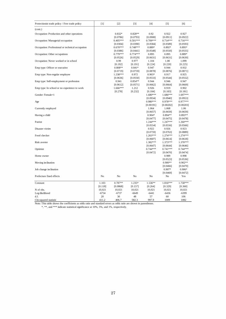
In our model, we also consider possible differences in preferences in terms of occupation
and employment type. However, the results of occupation and type of employment dummy variables
are not robust to the full model, including the non-economic attributes. Only the managerial
occupation dummy is still significant even if all the other factors are considered. People who are
engaged in managerial occupations are likely to support a free trade policy relative to people who are
engaged in other occupations. From the odds ratio, for the other occupation workers, the likelihood
of favoring a protectionist trade policy is 40% higher than people working in managerial occupations
(1/0.714 = 1.400). It is likely that non-regular employees are more likely to favor a protectionist
trade policy because they are easily affected by structural adjustments due to trade liberalization in
comparison with regular employees protected by strict restrictions on dismissal. Contrary to
expectations, the dummy for non-regular employees is not statistically significant, and therefore
there is no difference in the likelihood of favoring import restrictions between regular and
non-regular employees.
The non-economic characteristics show significant effects as reported in previous studies.
As an illustration, the gender dummy is strongly significant with a positive sign, showing that
females are more likely to prefer import restrictions than males. As a background, it is thought that
there is concern about the safety of imported food. To control for the effects of that concern, we add
a dummy variable for those who check additives and places of origin when purchasing food and
beverages. The gender dummy is still significant, although the effect of gender turns small when the
food check dummy is included. The odds ratio indicates that the probability of favoring import
restrictions for females is 1.7 times larger than for males. The odds ratio for food checkers is 27%
higher than for non-checkers. On the other hand, we find a negative correlation between age and
support for import restrictions. A one-year increase in age increases the probability of supporting a
free trade policy by 2%. Furthermore, people who have a child are likely to support a free trade
policy. The probability of favoring import restrictions for people who do not have a child is about
12% higher than for those who have a child. It is suggested that people are likely to decide to support
free trade policies when considering a next generation from a long-term perspective as expressed in
a dynasty model.
Previous studies demonstrate that personal political thought is also associated with trade
11
policy preferences.12 In our study, we add a dummy variable that takes a value of 1 for responses of
“strongly proud of one’s own country and hometown.” The result shows that people strongly proud
of their homeland are significantly more likely to favor import restrictions than others. There exists a
difference in preferences depending on attitude toward risk.13 Risk-averse people who do not buy a
lottery with a 50% chance to win tend to support import restrictions, possibly owing to the fear of
uncertainty associated with structural adjustment after trade liberalization. People with a pessimistic
view of Japan’s economy in the future are also likely to favor import restrictions. To control for an
inclination toward moving or job change, the mobility and job change dummies are added in
columns [5, 6]. As expected, people considering migration tend to support a free trade policy while
the job change dummy is insignificant. The other control variables, such as currently employed,
home ownership, and earthquake victim dummies, are not statistically significant. Overall, the strong
correlation between non-economic characteristics and trade policy preferences is observed from the
estimation results. Nevertheless, it is remarkable that the effects of regional factors are still
significant even after non-economic characteristics are included in the model.
3.2. Interaction of regional factors
The influence of regional characteristics may be different depending on an individual’s
attributes. Table 3 presents the results of interaction terms with respect to the ratio of agriculture
workers and the unemployment rate. The results of the other irrelevant covariates are suppressed
here. One may expect that the positive effect of the agricultural worker ratio in the region is more
pronounced in people who engage in the agricultural industry. To examine this, the interaction term
of the agricultural workers ratio and the industry affiliation dummy for agriculture industry is added
into the full model. Column [1] indicates that the interaction term has no effect on the trade policy
preferences, suggesting that people who reside in a region with a high concentration of agricultural
workers tend to be protectionist even if they engage in other sectors.
<Table 3. Results of interaction terms>
On the other hand, interestingly, it is found that the effect of agricultural workers ratio is offset for
people who are considering migration. This result can be seen in column [2], which includes the
interaction of agricultural workers ratio with the mobility dummy. The coefficient of the interaction
term is negative and significant, whereas the independent term of the agricultural workers ratio is
still positively significant. The odds ratio indicates that for people who are not considering migration,
12 As an illustration of this, Blonigen (2011) shows that democrats are more likely to favor a protectionist trade policy than republicans, using the U.S. individual-level data. 13 The effects of behavioral biases on trade policy preferences are further examined in Tomiura et al.
(2013).
12
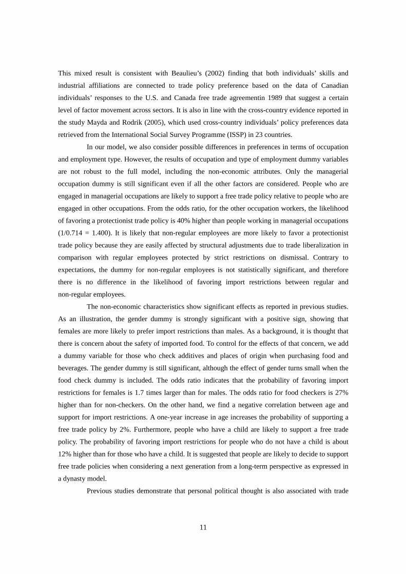
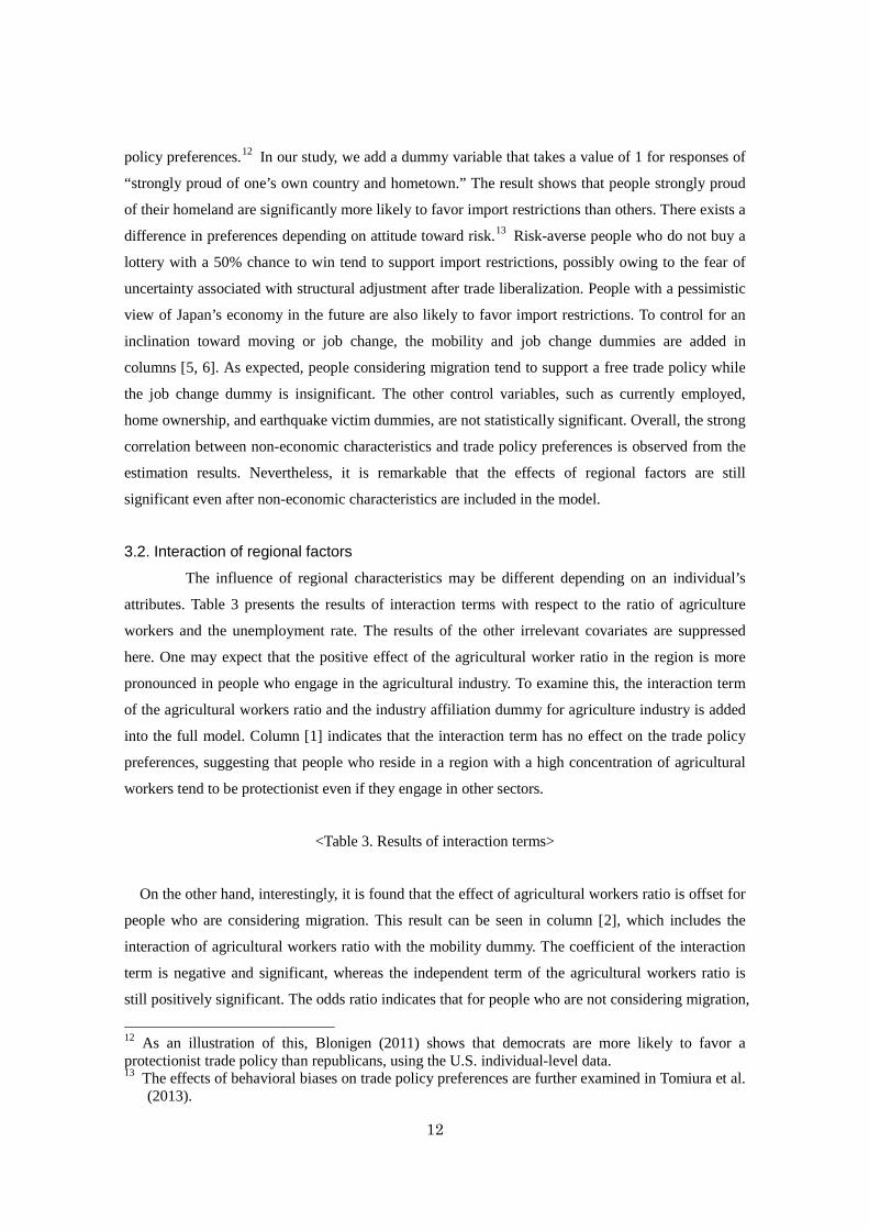
a one percentage point increase in the agricultural workers ratio is associated with a 2.5% increase in
the probability of supporting a protectionist trade policy. In contrast, for people who are considering
migration, the odds ratio turns out to be nearly a value of 1 from the calculation of the odds ratio of
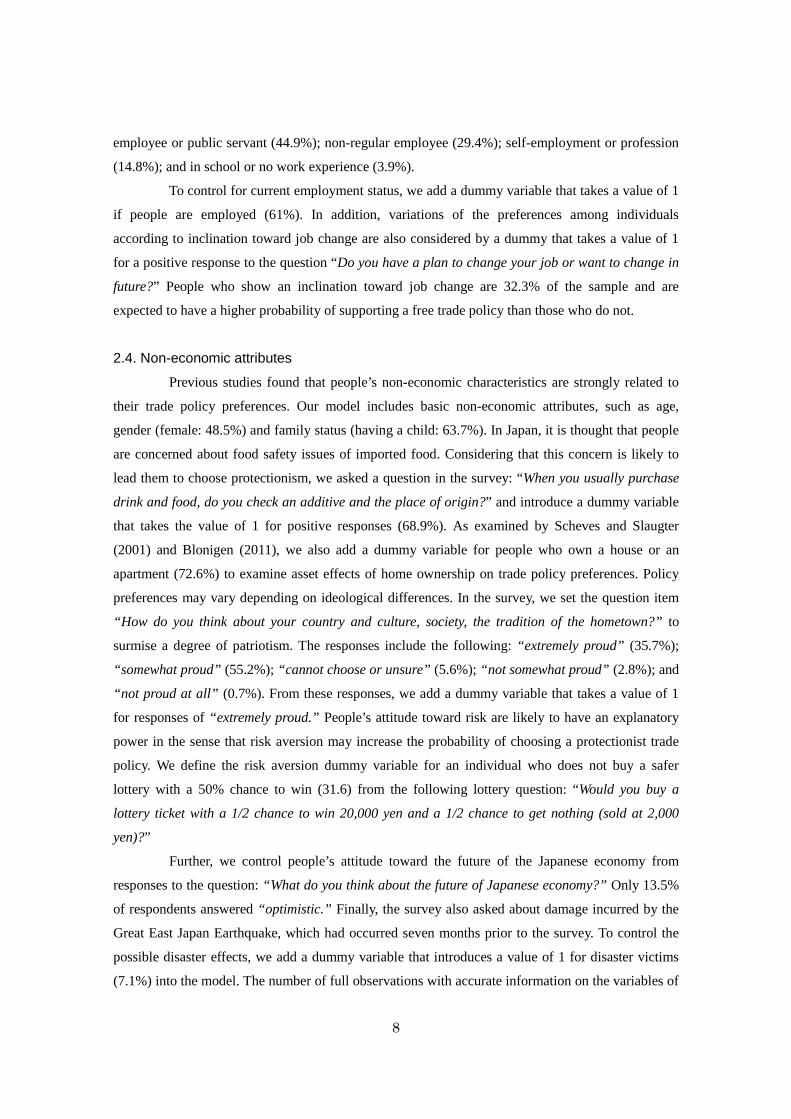
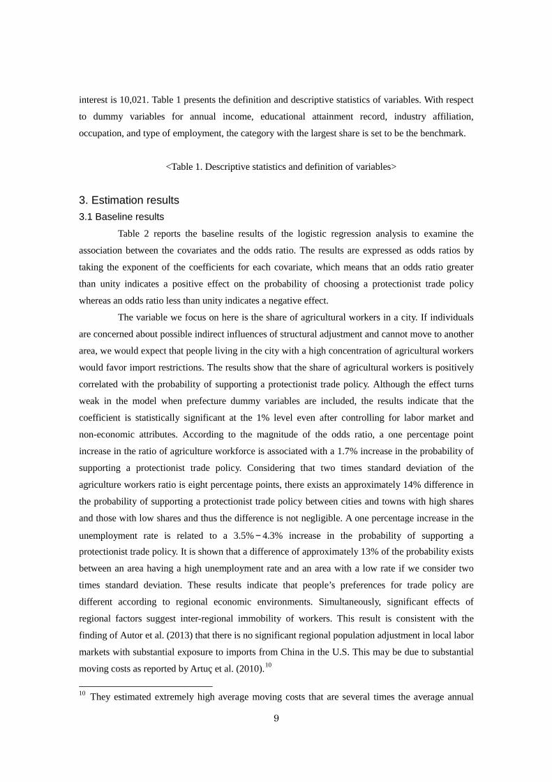
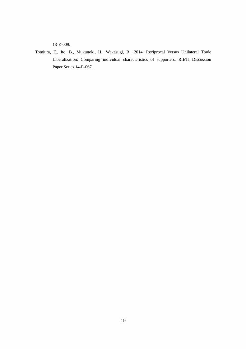
the interaction term multiplied by that of the independent term (1.025 × 0.998 = 0.994). To visualize
how the predicted probability differs according to the ratio of agricultural workers, Figure 2 shows
predictive margins by the mobility dummy at levels of the agricultural workers ratio from 0 through
75% at intervals of 5%. The vertical axis indicates the probability of supporting the protectionist
trade policy while the horizontal axis denotes the share of agricultural workers. As shown in the
results of the interaction term, although the probability tends to be higher for people who are not
considering migration, it does not change as a horizontal straight line for people who are considering
migration. The different result with the mobility dummy indicates the effect that the share of
agricultural workers in a region on people’s preference of trade policy focuses on people who do not
show an inclination toward migration.
<Figure 2. Predictive margins of mobility dummy given agricultural workers share>
Next, we introduce the interaction term between the home ownership dummy and the share
of agricultural workers in a region into column [3] to examine possible heterogeneity of asset effects
on trade policy preferences. However, such heterogeneity is not observed. Instead, it is found that the
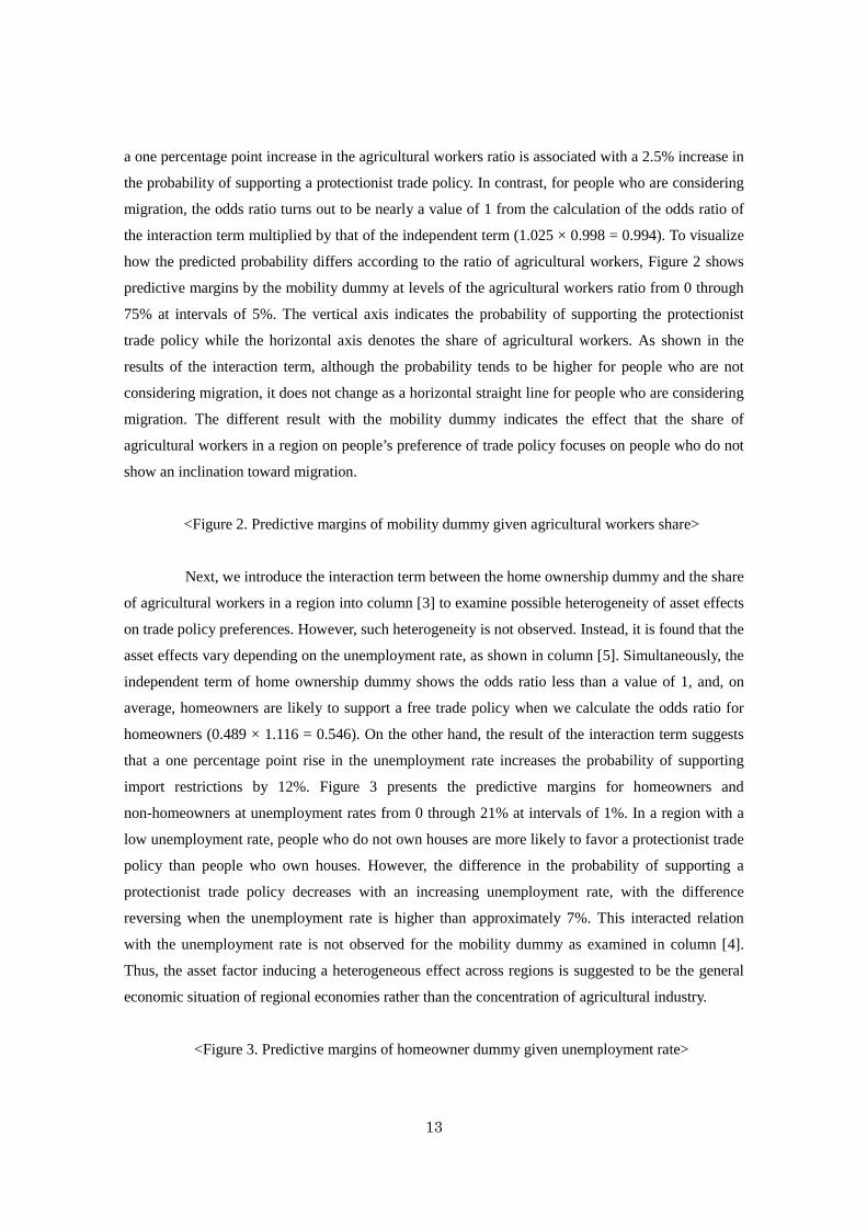
asset effects vary depending on the unemployment rate, as shown in column [5]. Simultaneously, the
independent term of home ownership dummy shows the odds ratio less than a value of 1, and, on
average, homeowners are likely to support a free trade policy when we calculate the odds ratio for
homeowners (0.489 × 1.116 = 0.546). On the other hand, the result of the interaction term suggests
that a one percentage point rise in the unemployment rate increases the probability of supporting
import restrictions by 12%. Figure 3 presents the predictive margins for homeowners and
non-homeowners at unemployment rates from 0 through 21% at intervals of 1%. In a region with a
low unemployment rate, people who do not own houses are more likely to favor a protectionist trade
policy than people who own houses. However, the difference in the probability of supporting a
protectionist trade policy decreases with an increasing unemployment rate, with the difference
reversing when the unemployment rate is higher than approximately 7%. This interacted relation
with the unemployment rate is not observed for the mobility dummy as examined in column [4].
Thus, the asset factor inducing a heterogeneous effect across regions is suggested to be the general
economic situation of regional economies rather than the concentration of agricultural industry.
<Figure 3. Predictive margins of homeowner dummy given unemployment rate>
13
The above-mentioned results are based on a broad definition by which the individuals who
answered “cannot choose or unsure” are assigned to those who support import restrictions. To check the consistency of these results, we also estimate the same equation based on an alternative definition, which excludes these individuals from the sample. As a result, 8,327 individuals remained in the sample. As shown in Appendix Tables A1 and A2, the main results are not changed. In addition, a similar result is obtained for interaction terms as drawn in Appendix
Figures A1 and A2.
4. Robustness check: multilevel mixed logistic regression
In addition to the standard logistic regression, as a robustness check, we further estimate a
multilevel mixed logistic regression that considers unobserved heterogeneity across regions. To
control for regional heterogeneity, we can estimate by introducing the interaction of region dummy
variables and covariates with region dummies. However, this is difficult to handle when many
regions exist in the data. Furthermore, if trade policy preferences among individuals in the same
region are similar, it is anticipated that potential endogeneity in the sense that regional factors in
common with individuals in the same region are correlated with individual factors, generating biased
coefficients. A multilevel model approach enables us to separate unobserved regional heterogeneity
of trade policy preference from the error term by adding random effects into linear predictors. In the
robustness check, we estimate the two-level model comprising individual-level and regional–level
data. Regarding the regional level, we consider both prefecture-level and city–level data. Following
Raudenbush and Bryk (2002), the two-level mixed logistic model is specified as below. At level 1,
which is set at individual level, the latent variable is determined by the following equation:
ijijjijjij ezxy +++= γββ 10* , (4)
where ijx is a set of variables and its coefficients are assumed to be fixed across all individuals,
whereas the intercept j0β and coefficients of ijz randomly vary across regions. Hence, the second
level of the two-level model is written as
jj u000 += ββ , (5)
jj u11 += γγ , (6)
where 0β is the intercept that is common across individuals and ju0 is the random intercept
14
that varies across regions. Similarly, 1γ is the fixed coefficient for all individuals while ju1 is a
random coefficient, which can be different depending on the region. The random effects are assumed
to be independent and identically distributed across regions and independent of the covariates. The
error term in the first level is assumed to be a logistic distribution. Combining the two-level
equations, the model for the latent variable can be specified as a mix of fixed and random effects:
ijijjjijijij ezuuzxy +++++= 101,110* γββ . (7)
Various models are included in the estimation. As for the random coefficients model,
because random coefficients are not known beforehand, we estimate them individually and examine
the statistical significance of the random coefficient by the likelihood ratio test. The insignificance of
random coefficients supports that the fixed effects are plausible. The fixed effects can be interpreted
by the odds ratio as the standard logistic regression.14
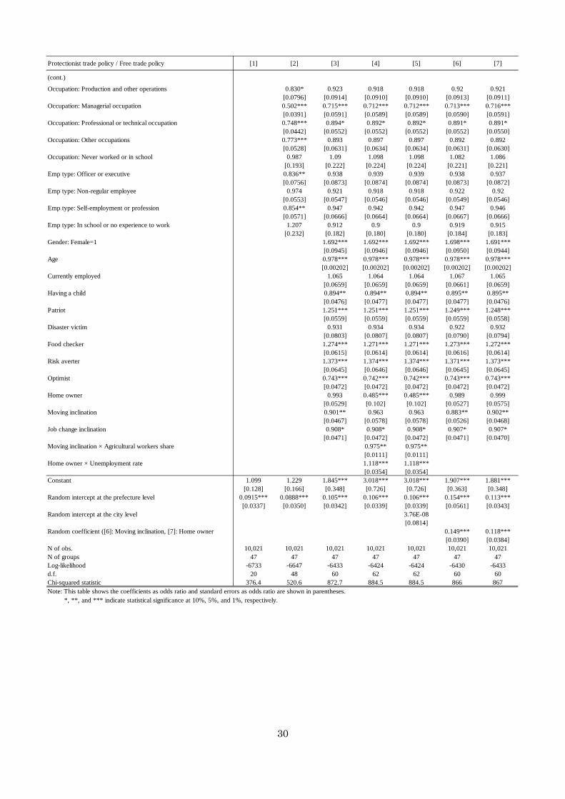
The results of the random intercept model are reported in Table 4. The models have a
random intercept at the prefecture level as a two-level model, except for column [5], which includes
a random intercept at both the prefecture and city levels as a three-level model. As for fixed effects,
the figures in the table show that the odds ratio can correspond to a one unit change in the
explanatory variable. The results of the likelihood ratio tests for model selection support the
multilevel model rather than logistic regression model while the estimated coefficients are similar to
those from the standard logistic regression model. It is remarkable that the regional factors, the share
of agricultural workers, and the unemployment rate still have a positive and significant relationship
with the probability of supporting a protectionist trade policy.
<Table 4. Results of multilevel mixed logistic regression>
After estimating the random intercept model, the result from the estimated standard
deviation of random intercept shows that individuals’ trade policy preferences are different among
prefectures. In contrast, the heterogeneity of trade policy preferences across cities is not observed
from the results of the three-level model, which has a random intercept at the prefecture and city
levels. Figure 4 shows how different the random intercepts are depending on the prefectures.
14 The multilevel mixed logistic model is estimated by maximum likelihood estimation. However, since the joint probability includes the integral of random effects, the model does not have a closed-form solution. We apply the Gauss–Hermite quadrature approximation to the random effect to replace the continuous density by a discrete distribution.
15
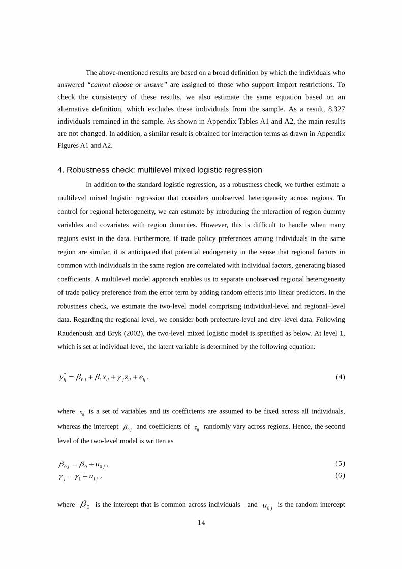
Although the multilevel model suggests that unobserved prefecture-specific factors affect individuals’
trade policy preferences, the results of an intra-class correlation coefficient in terms of residuals
calculated as the proportion of variance explained are 0.006–0.01, showing that the magnitude of the random intercept at the prefecture level turns out to be marginal. This means that most of the
variance can be explained by the fixed effects of the covariates.
<Figure 4. Unobserved heterogeneity in trade policy preferences across prefectures>
Next, we investigate the difference in the impacts of covariates across the prefectures. To
identify the variable that has a random coefficient, we estimate a random coefficient model
individually for each explanatory variable. As a result, it is found that a random coefficient model is
appropriate only for two variables: mobility and home ownership dummies. Column [6] shows the
result of the random intercept and random coefficient models in terms of the mobility dummy
variable, and column [7] displays that for the home ownership dummy. These results uphold that the
coefficient varies depending on prefecture, which is consistent with the results of the interaction
terms with regional factors. It is interesting to see difference in the coefficient of the mobility
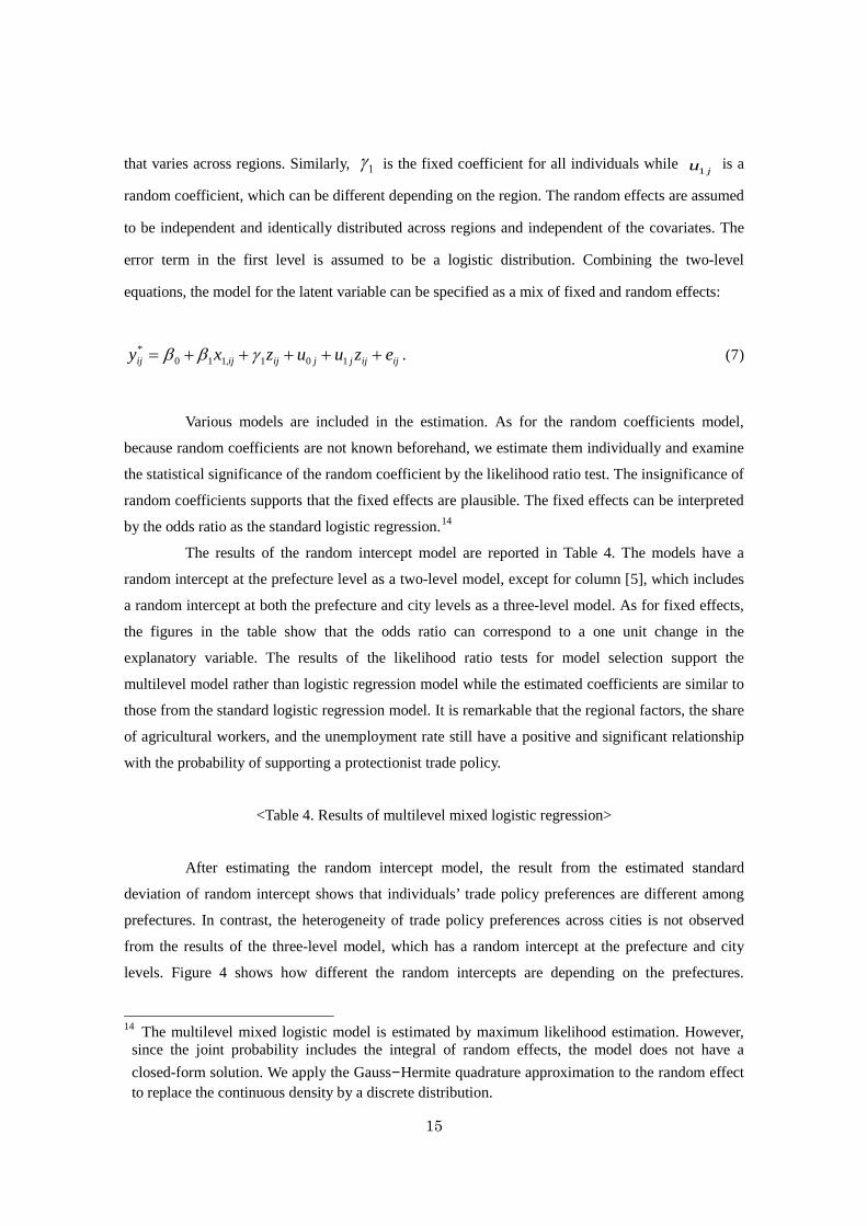
dummy according to prefectures. Figure 5 displays the summation of the fixed coefficient and the
random coefficient on the mobility dummy over prefectures. In most prefectures, people who are
considering migration tend to support a free trade policy, although the magnitude is considerably
different across them. It seems that the positive effect of an inclination toward migration on the
probability of supporting a free trade policy is more pronounced for people who reside in a local
area.
<Figure 5. Regional differences in effect of inclination toward moving>
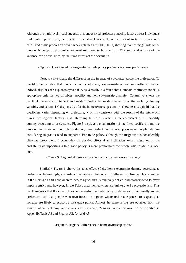
Similarly, Figure 6 shows the total effect of the home ownership dummy according to
prefectures. Interestingly, a significant variation in the random coefficient is observed. For example,
in the Hokkaido and Tohoku areas, where agriculture is relatively active, homeowners tend to favor
import restrictions; however, in the Tokyo area, homeowners are unlikely to be protectionists. This
result suggests that the effect of home ownership on trade policy preferences differs greatly among
prefectures and that people who own houses in regions where real estate prices are expected to
increase are likely to support a free trade policy. Almost the same results are obtained from the
sample when excluding individuals who answered “cannot choose or unsure” as reported in
Appendix Table A3 and Figures A3, A4, and A5.
<Figure 6. Regional differences in home ownership effect>
16
5. Concluding remarks Previous studies explored the determinants of individuals’ trade policy preferences by
focusing on individuals’ skill endowments and industrial attributes to examine the mobility of
workers across industries. It has been reported that these labor market attributes are related to
individual’s trade policy preferences; however, as noted by Blonigen (2011), it is difficult to explain
trade policy preferences only by the labor market attributes. In this study, we conducted an empirical
study on, in particular, the association between regional factors and trade policy preferences, which
very few have attempted, and employed individual-level data from ten thousand people from a wide
range of areas of Japan.
The results of binary choice model reveal that regional characteristics, such as the share of
agricultural workers and the unemployment rate on protectionist trade policies, have a significant
impact on trade policy preferences. More specifically, as the agricultural workers ratio and the
unemployment rate increase, people tend to be protectionists even if they do not engage in
agriculture. In Japan’s local areas, where key industries include agriculture, other industries, such as
food processing and manufacturing that produces agricultural equipment may be indirectly affected
by structural reforms following trade liberalization. It is suggested that an individual chooses a trade
policy preference by considering such industrial linkage effects in areas with a high concentration of
import-competing industries. Interestingly, the positive impact of local agricultural workers share on
a support for import restrictions is offset by people who are considering migration. These results are
very stable even when we add labor market and non-economic attributes. Further, the results are
robust to a multilevel mixed logistic regression model that considers unobserved region-specific
factors. Taken together, it is concluded that people’s trade policy preferences react to whether they
are mobile between regions. Considering the fact that the effects of regional factors are remarkable,
it is suggested that the inter-regional immobility can be an important factor in increasing the support
for protectionist trade policies.
From our results, it is concluded that trade policy preferences react sensitively with
inter-regional mobility. Until now, it has been highlighted that it is important to promote trade
liberalization to increase the mobility of human resources in labor markets; however, a consensus on
a free trade policy cannot be reached based only on the mobility of human resources between sectors,
considering the difficulty of moving between regions. To build consensus for further trade
liberalization, it is necessary to find ways to stimulate development of new or service industries in
regions where comparatively disadvantaged tradable industries are concentrated.
17
References Artuç, E., Chaudhuri, S., McLaren, J., 2010. Trade shocks and labor adjustment: A structural
empirical approach. American Economic Review 100(3), 1008–45.
Autor, D.H., Dorn, D., Hanson, G.H., 2013. The China syndrome: Local labor market effects of
import competition in the United States. American Economic Review 103(6), 2121–2168.
Baldwin, R.E., Magee, C.S., 2000. Is trade policy for sale? Congressional voting on recent trade bills.
Public Choice 105, 79–101.
Beaulieu, E., 2002a. Factor or industry cleavages in trade policy? An empirical analysis of the
Stolper–Samuelson theorem. Economics and Politics 14, 99–131.
Beaulieu, E., 2002b. The Stolper–Samuelson theorem faces congress. Review of International
Economics 10, 343–360.
Blonigen, B., 2011. Revisiting the evidence on trade policy preferences. Journal of International
Economics 85, 129–135.
Davis, C., 2004. International institutions and issue linkages: Building support for agriculture trade
liberalization. American Political Science Review 98(1), 153–169.
Evans, C.L., 2009. A protectionist bias in majoritarian politics: An empirical investigation.
Economics and Politics 21, 278–307.
Fredriksson, Per G., Matschke, X., Minier, J., 2010. Trade policy in majoritarian systems: The case
of the U.S. Canadian Journal of Economics 44, 607–626.
Goldberg, P. K., Maggi, G., 1999. Protection for sale: An empirical investigation. American
Economic Review 89(5), 1135–55.
Grossman, G., Helpman, E., 1994. Protection for sale. American Economic Review 84, 833–850.
Grossman, G., Helpman, E., 2005. A protectionist bias in majoritarian politics. Quarterly Journal of
Economics 120, 1239–1282.
Kaempfer, W.H., Marks, S.V., 1993. The expected effects of trade liberalization: evidence from US
congressional action on fast-track authority. World Economy 16, 725–740.
Mayda, A., Rodrik, D., 2005. Why are some people (and countries) more protectionist than others?
European Economic Review 49, 1393–1430.
McCalman, P., 2004. Protection for sale and trade liberalization: An empirical investigation. Review
of International Economics 74(1), 372–382.
Raudenbush, S. W., Bryk, A. S., 2002. Hierarchical Linear Models: Applications and Data Analysis
Methods. 2nd edition. Thousand Oaks, CA: Sage.
Scheve, K., Slaughter, M., 2001. What determines individual trade-policy preferences? Journal of
International Economics 54, 267–292.
Tomiura, E., Ito, B., Mukunoki, H., Wakasugi, R., 2013. Endowment Effect and Trade Policy
Preferences: Evidence from a survey on individuals. RIETI Discussion Paper Series
18
13-E-009.
Tomiura, E., Ito, B., Mukunoki, H., Wakasugi, R., 2014. Reciprocal Versus Unilateral Trade
Liberalization: Comparing individual characteristics of supporters. RIETI Discussion
Paper Series 14-E-067.
19
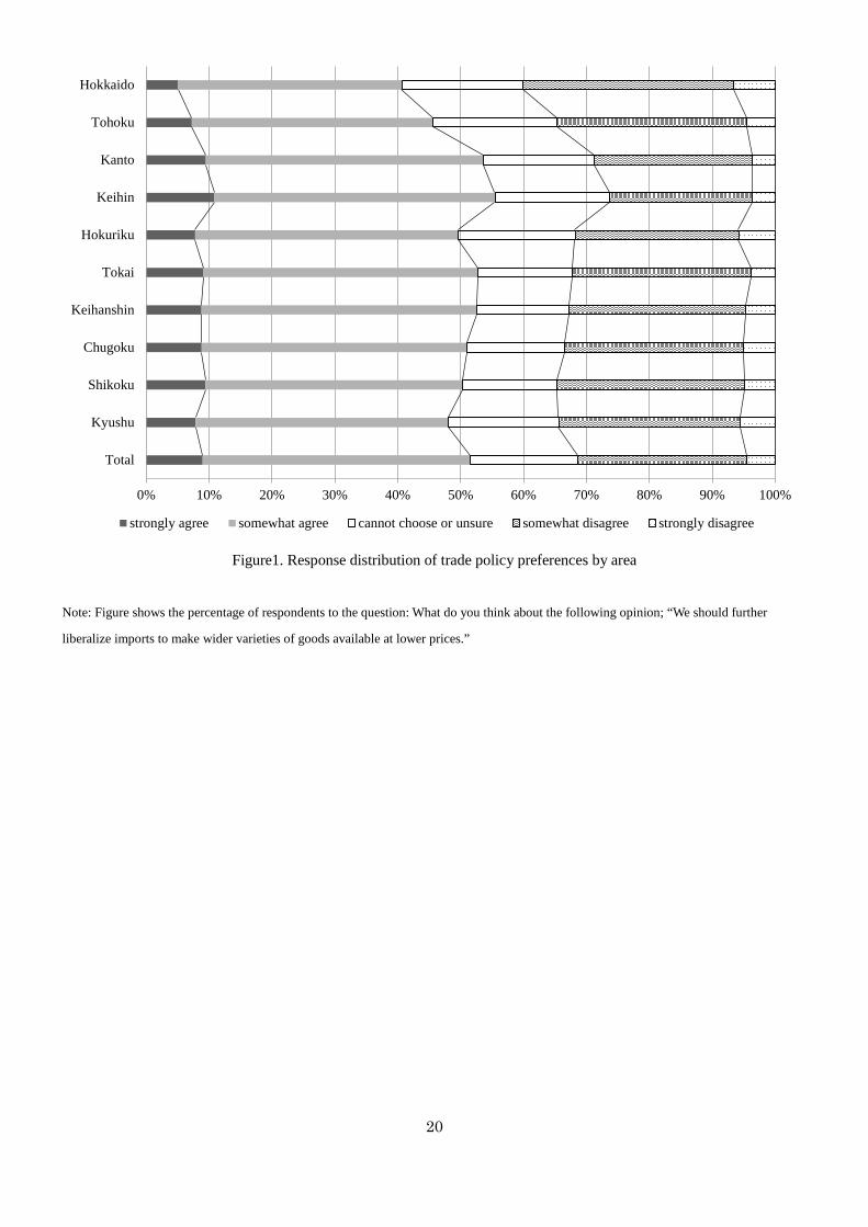
Figure1. Response distribution of trade policy preferences by area
Note: Figure shows the percentage of respondents to the question: What do you think about the following opinion; “We should further
liberalize imports to make wider varieties of goods available at lower prices.”
0% 10% 20% 30% 40% 50% 60% 70% 80% 90% 100%
Total
Kyushu
Shikoku
Chugoku
Keihanshin
Tokai
Hokuriku
Keihin
Kanto
Tohoku
Hokkaido
strongly agree somewhat agree cannot choose or unsure somewhat disagree strongly disagree
20
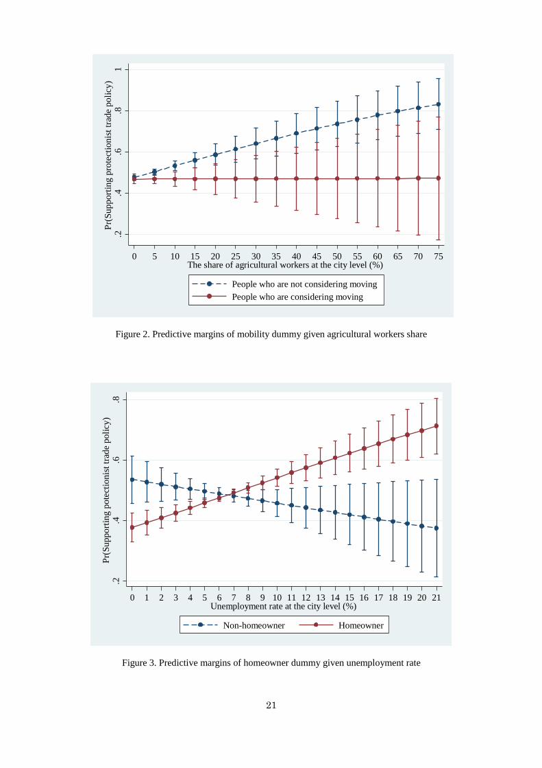
Figure 2. Predictive margins of mobility dummy given agricultural workers share
Figure 3. Predictive margins of homeowner dummy given unemployment rate
.2.4
.6.8
1Pr
(Sup
porti
ng p
rote
ctio
nist
trad
e po
licy)
0 5 10 15 20 25 30 35 40 45 50 55 60 65 70 75The share of agricultural workers at the city level (%)
People who are not considering movingPeople who are considering moving
.2.4
.6.8
Pr(S
uppo
rting
pot
ectio
nist
trad
e po
licy)
0 1 2 3 4 5 6 7 8 9 10 11 12 13 14 15 16 17 18 19 20 21Unemployment rate at the city level (%)
Non-homeowner Homeowner
21
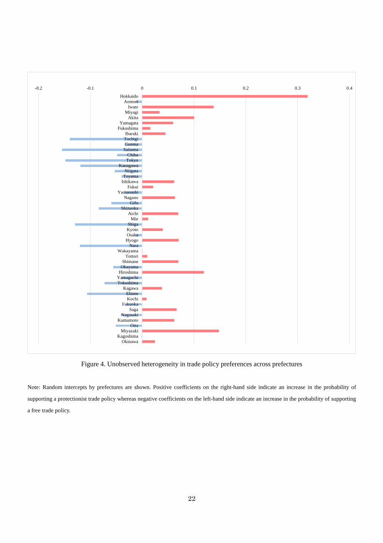
Figure 4. Unobserved heterogeneity in trade policy preferences across prefectures
Note: Random intercepts by prefectures are shown. Positive coefficients on the right-hand side indicate an increase in the probability of
supporting a protectionist trade policy whereas negative coefficients on the left-hand side indicate an increase in the probability of supporting
a free trade policy.
-0.2 -0.1 0 0.1 0.2 0.3 0.4
HokkaidoAomori
IwateMiyagi
AkitaYamagata
FukushimaIbaraki
TochigiGunma
SaitamaChibaTokyo
KanagawaNiigata
ToyamaIshikawa
FukuiYamanashi
NaganoGifu
ShizuokaAichi
MieShigaKyotoOsakaHyogo
NaraWakayama
TottoriShimane
OkayamaHiroshima
YamaguchiTokushima
KagawaEhimeKochi
FukuokaSaga
NagasakiKumamoto
OitaMiyazaki
KagoshimaOkinawa
22
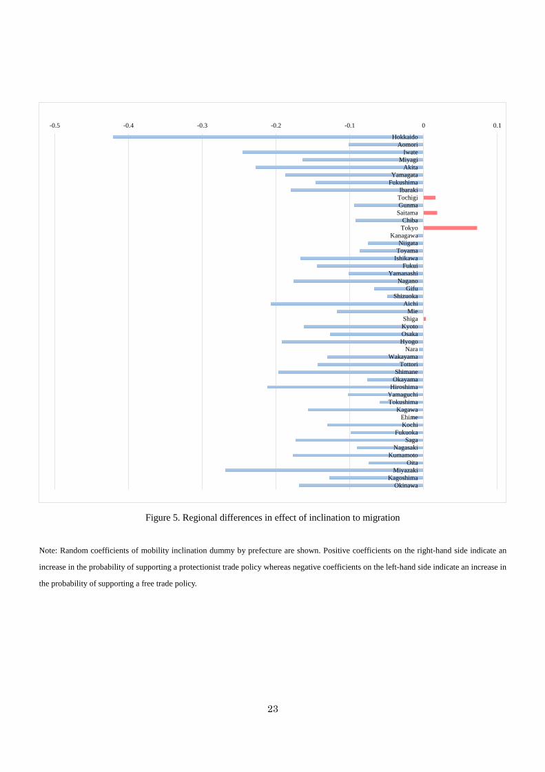
Figure 5. Regional differences in effect of inclination to migration
Note: Random coefficients of mobility inclination dummy by prefecture are shown. Positive coefficients on the right-hand side indicate an
increase in the probability of supporting a protectionist trade policy whereas negative coefficients on the left-hand side indicate an increase in
the probability of supporting a free trade policy.
-0.5 -0.4 -0.3 -0.2 -0.1 0 0.1
HokkaidoAomori
IwateMiyagi
AkitaYamagata
FukushimaIbaraki
TochigiGunma
SaitamaChibaTokyo
KanagawaNiigata
ToyamaIshikawa
FukuiYamanashi
NaganoGifu
ShizuokaAichi
MieShigaKyotoOsakaHyogo
NaraWakayama
TottoriShimane
OkayamaHiroshima
YamaguchiTokushima
KagawaEhimeKochi
FukuokaSaga
NagasakiKumamoto
OitaMiyazaki
KagoshimaOkinawa
23
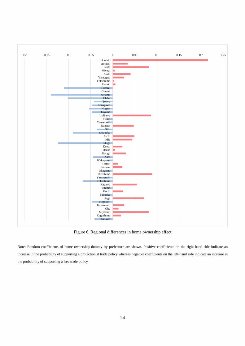
Figure 6. Regional differences in home ownership effect
Note: Random coefficients of home ownership dummy by prefecture are shown. Positive coefficients on the right-hand side indicate an
increase in the probability of supporting a protectionist trade policy whereas negative coefficients on the left-hand side indicate an increase in
the probability of supporting a free trade policy.
-0.2 -0.15 -0.1 -0.05 0 0.05 0.1 0.15 0.2 0.25
HokkaidoAomori
IwateMiyagi
AkitaYamagata
FukushimaIbaraki
TochigiGunma
SaitamaChibaTokyo
KanagawaNiigata
ToyamaIshikawa
FukuiYamanashi
NaganoGifu
ShizuokaAichi
MieShigaKyotoOsakaHyogo
NaraWakayama
TottoriShimane
OkayamaHiroshima
YamaguchiTokushima
KagawaEhimeKochi
FukuokaSaga
NagasakiKumamoto
OitaMiyazaki
KagoshimaOkinawa
24
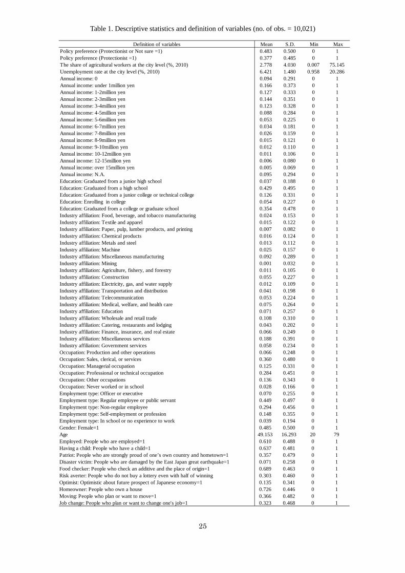
Table 1. Descriptive statistics and definition of variables (no. of obs. = 10,021)
Definition of variables Mean S.D. Min MaxPolicy preference (Protectionist or Not sure =1) 0.483 0.500 0 1Policy preference (Protectionist =1) 0.377 0.485 0 1The share of agricultural workers at the city level (%, 2010) 2.778 4.030 0.007 75.145Unemployment rate at the city level (%, 2010) 6.421 1.480 0.958 20.286Annual income: 0 0.094 0.291 0 1Annual income: under 1million yen 0.166 0.373 0 1Annual income: 1-2million yen 0.127 0.333 0 1Annual income: 2-3million yen 0.144 0.351 0 1Annual income: 3-4million yen 0.123 0.328 0 1Annual income: 4-5million yen 0.088 0.284 0 1Annual income: 5-6million yen 0.053 0.225 0 1Annual income: 6-7million yen 0.034 0.181 0 1Annual income: 7-8million yen 0.026 0.159 0 1Annual income: 8-9million yen 0.015 0.121 0 1Annual income: 9-10million yen 0.012 0.110 0 1Annual income: 10-12million yen 0.011 0.106 0 1Annual income: 12-15million yen 0.006 0.080 0 1Annual income: over 15million yen 0.005 0.069 0 1Annual income: N.A. 0.095 0.294 0 1Education: Graduated from a junior high school 0.037 0.188 0 1Education: Graduated from a high school 0.429 0.495 0 1Education: Graduated from a junior college or technical college 0.126 0.331 0 1Education: Enrolling in college 0.054 0.227 0 1Education: Graduated from a college or graduate school 0.354 0.478 0 1Industry affiliation: Food, beverage, and tobacco manufacturing 0.024 0.153 0 1Industry affiliation: Textile and apparel 0.015 0.122 0 1Industry affiliation: Paper, pulp, lumber products, and printing 0.007 0.082 0 1Industry affiliation: Chemical products 0.016 0.124 0 1Industry affiliation: Metals and steel 0.013 0.112 0 1Industry affiliation: Machine 0.025 0.157 0 1Industry affiliation: Miscellaneous manufacturing 0.092 0.289 0 1Industry affiliation: Mining 0.001 0.032 0 1Industry affiliation: Agriculture, fishery, and forestry 0.011 0.105 0 1Industry affiliation: Construction 0.055 0.227 0 1Industry affiliation: Electricity, gas, and water supply 0.012 0.109 0 1Industry affiliation: Transportation and distribution 0.041 0.198 0 1Industry affiliation: Telecommunication 0.053 0.224 0 1Industry affiliation: Medical, welfare, and health care 0.075 0.264 0 1Industry affiliation: Education 0.071 0.257 0 1Industry affiliation: Wholesale and retail trade 0.108 0.310 0 1Industry affiliation: Catering, restaurants and lodging 0.043 0.202 0 1Industry affiliation: Finance, insurance, and real estate 0.066 0.249 0 1Industry affiliation: Miscellaneous services 0.188 0.391 0 1Industry affiliation: Government services 0.058 0.234 0 1Occupation: Production and other operations 0.066 0.248 0 1Occupation: Sales, clerical, or services 0.360 0.480 0 1Occupation: Managerial occupation 0.125 0.331 0 1Occupation: Professional or technical occupation 0.284 0.451 0 1Occupation: Other occupations 0.136 0.343 0 1Occupation: Never worked or in school 0.028 0.166 0 1Employment type: Officer or executive 0.070 0.255 0 1Employment type: Regular employee or public servant 0.449 0.497 0 1Employment type: Non-regular employee 0.294 0.456 0 1Employment type: Self-employment or profession 0.148 0.355 0 1Employment type: In school or no experience to work 0.039 0.194 0 1Gender: Female=1 0.485 0.500 0 1Age 49.153 16.293 20 79Employed: People who are employed=1 0.610 0.488 0 1Having a child: People who have a child=1 0.637 0.481 0 1Patriot: People who are strongly proud of one’s own country and hometown=1 0.357 0.479 0 1Disaster victim: People who are damaged by the East Japan great earthquake=1 0.071 0.258 0 1Food checker: People who check an additive and the place of origin=1 0.689 0.463 0 1Risk averter: People who do not buy a lottery even with half of winning 0.303 0.460 0 1Optimist: Optimistic about future prospect of Japanese economy=1 0.135 0.341 0 1Homeowner: People who own a house 0.726 0.446 0 1Moving: People who plan or want to move=1 0.366 0.482 0 1Job change: People who plan or want to change one's job=1 0.323 0.468 0 1
25
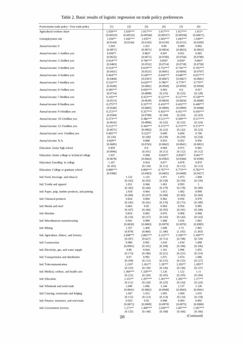
Table 2. Basic results of logistic regression on trade policy preferences
Protectionist trade policy / Free trade policy [1] [2] [3] [4] [5] [6]
Agricultural workers share 1.020*** 1.020*** 1.017*** 1.017*** 1.017*** 1.011*[0.00525] [0.00535] [0.00540] [0.00557] [0.00558] [0.00671]
Unemployment rate 1.036** 1.042*** 1.035** 1.043*** 1.043*** 1.049**[0.0144] [0.0144] [0.0145] [0.0150] [0.0151] [0.0209]
Annual income: 0 1.043 1.021 0.89 0.889 0.892[0.0871] [0.0871] [0.0824] [0.0823] [0.0832]
Annual income: 1-2million yen 0.830** 0.865* 0.947 0.951 0.965[0.0632] [0.0671] [0.0760] [0.0764] [0.0780]
Annual income: 2-3million yen 0.654*** 0.706*** 0.856* 0.859* 0.865*[0.0483] [0.0552] [0.0714] [0.0718] [0.0728]
Annual income: 3-4million yen 0.554*** 0.619*** 0.753*** 0.756*** 0.765***[0.0431] [0.0521] [0.0691] [0.0694] [0.0707]
Annual income: 4-5million yen 0.464*** 0.538*** 0.650*** 0.648*** 0.657***[0.0404] [0.0507] [0.0667] [0.0667] [0.0681]
Annual income: 5-6million yen 0.532*** 0.618*** 0.780** 0.779** 0.779**[0.0549] [0.0681] [0.0930] [0.0930] [0.0938]
Annual income: 6-7million yen 0.585*** 0.693*** 0.903 0.9 0.917[0.0714] [0.0898] [0.125] [0.125] [0.128]
Annual income: 7-8million yen 0.356*** 0.423*** 0.521*** 0.517*** 0.528***[0.0513] [0.0639] [0.0829] [0.0824] [0.0848]
Annual income: 8-9million yen 0.275*** 0.337*** 0.433*** 0.432*** 0.449***[0.0540] [0.0685] [0.0909] [0.0909] [0.0948]
Annual income: 9-10million yen 0.272*** 0.357*** 0.455*** 0.451*** 0.450***[0.0584] [0.0788] [0.104] [0.103] [0.103]
Annual income: 10-12million yen 0.273*** 0.386*** 0.511*** 0.509*** 0.517***[0.0616] [0.0896] [0.122] [0.122] [0.124]
Annual income: 12-15million yen 0.212*** 0.304*** 0.372*** 0.373*** 0.373***[0.0671] [0.0982] [0.122] [0.122] [0.123]
Annual income: over 15million yen 0.405*** 0.522** 0.699 0.694 0.706[0.126] [0.168] [0.230] [0.229] [0.234]
Annual income: N.A. 0.829** 0.898 0.953 0.952 0.956[0.0685] [0.0765] [0.0842] [0.0841] [0.0851]
Education: Junior high school 0.859 0.9 0.969 0.972 0.965[0.0946] [0.101] [0.111] [0.112] [0.112]
Education: Junior college or technical college 1.037 0.998 0.856** 0.858** 0.861**[0.0678] [0.0662] [0.0583] [0.0584] [0.0590]
Education: Enrolling in college 1.107 0.954 0.877 0.878 0.879[0.105] [0.118] [0.112] [0.112] [0.113]
Education: College or graduate school 0.800*** 0.800*** 0.767*** 0.773*** 0.782***[0.0386] [0.0403] [0.0405] [0.0408] [0.0417]
Ind: Food, beverage, and tobacco 1.122 1.125 1.071 1.073 1.068[0.162] [0.163] [0.158] [0.159] [0.159]
Ind: Textile and apparel 1.051 0.946 1.001 0.993 1[0.182] [0.166] [0.179] [0.178] [0.180]
Ind: Paper, pulp, lumber products, and printing 1.018 0.964 1.013 1.002 0.999[0.260] [0.247] [0.268] [0.265] [0.264]
Ind: Chemical products 0.824 0.894 0.962 0.956 0.978[0.145] [0.161] [0.176] [0.175] [0.180]
Ind: Metals and steel 0.863 0.85 0.964 0.956 0.985[0.167] [0.166] [0.192] [0.191] [0.198]
Ind: Machine 0.819 0.892 0.976 0.968 0.968[0.116] [0.127] [0.143] [0.142] [0.143]
Ind: Miscellaneous manufacturing 0.941 0.989 1.068 1.056 1.063[0.0830] [0.0883] [0.0979] [0.0970] [0.0985]
Ind: Mining 1.357 1.469 1.698 1.72 1.865[0.879] [0.966] [1.180] [1.192] [1.303]
Ind: Agriculture, fishery, and forestry 2.698*** 2.805*** 3.133*** 3.109*** 3.169***[0.597] [0.627] [0.713] [0.708] [0.729]
Ind: Construction 0.986 0.991 1.034 1.034 1.008[0.0991] [0.101] [0.108] [0.108] [0.106]
Ind: Electricity, gas, and water supply 0.89 0.944 1.101 1.096 1.055[0.173] [0.186] [0.221] [0.221] [0.214]
Ind: Transportation and distribution 0.97 0.992 1.075 1.074 1.086[0.109] [0.112] [0.125] [0.125] [0.127]
Ind: Telecommunication 1.210* 1.261** 1.287** 1.292** 1.285**[0.123] [0.130] [0.136] [0.136] [0.137]
Ind: Medical, welfare, and health care 1.360*** 1.328*** 1.126 1.122 1.11[0.121] [0.120] [0.105] [0.105] [0.104]
Ind: Education 1.225** 1.297*** 1.301*** 1.285*** 1.277**[0.111] [0.120] [0.125] [0.124] [0.124]
Ind: Wholesale and retail trade 1.049 1.066 1.144 1.137 1.126[0.0841] [0.0862] [0.0948] [0.0943] [0.0941]
Ind: Catering, restaurants and lodging 1.047 1.015 1.005 1.004 1.035[0.115] [0.113] [0.114] [0.114] [0.118]
Ind: Finance, insurance, and real estate 0.923 0.95 0.998 0.993 0.992[0.0871] [0.0909] [0.0979] [0.0975] [0.0980]
Ind: Government services 1.271** 1.400*** 1.630*** 1.607*** 1.587***[0.125] [0.140] [0.168] [0.166] [0.166]
(Continued) 26
Protectionist trade policy / Free trade policy [1] [2] [3] [4] [5] [6]
(cont.)
Occupation: Production and other operations 0.832* 0.828** 0.92 0.922 0.927[0.0786] [0.0793] [0.0908] [0.0911] [0.0922]
Occupation: Managerial occupation 0.405*** 0.501*** 0.709*** 0.714*** 0.716***[0.0304] [0.0390] [0.0584] [0.0589] [0.0593]
Occupation: Professional or technical occupation 0.670*** 0.748*** 0.889* 0.892* 0.895*[0.0386] [0.0441] [0.0548] [0.0550] [0.0555]
Occupation: Other occupations 0.779*** 0.774*** 0.895 0.895 0.889*[0.0526] [0.0529] [0.0631] [0.0631] [0.0630]
Occupation: Never worked or in school 0.99 0.977 1.104 1.08 1.099[0.192] [0.191] [0.224] [0.220] [0.225]
Emp type: Officer or executive 0.808** 0.841* 0.947 0.944 0.932[0.0719] [0.0759] [0.0878] [0.0876] [0.0871]
Emp type: Non-regular employee 1.238*** 0.972 0.903* 0.917 0.925[0.0636] [0.0550] [0.0533] [0.0544] [0.0552]
Emp type: Self-employment or profession 0.941 0.854** 0.944 0.946 0.947[0.0612] [0.0571] [0.0662] [0.0664] [0.0669]
Emp type: In school or no experience to work 1.666*** 1.212 0.926 0.919 0.902[0.278] [0.232] [0.184] [0.183] [0.181]
Gender: Female=1 1.680*** 1.686*** 1.697***[0.0934] [0.0940] [0.0953]
Age 0.980*** 0.978*** 0.977***[0.00191] [0.00202] [0.00203]
Currently employed 1.064 1.068 1.06[0.0657] [0.0659] [0.0659]
Having a child 0.904* 0.894** 0.893**[0.0477] [0.0475] [0.0478]
Patriot 1.244*** 1.247*** 1.260***[0.0554] [0.0556] [0.0566]
Disaster victim 0.922 0.926 0.923[0.0759] [0.0763] [0.0889]
Food checker 1.263*** 1.274*** 1.274***[0.0607] [0.0614] [0.0618]
Risk averter 1.382*** 1.373*** 1.370***[0.0647] [0.0644] [0.0646]
Optimist 0.744*** 0.741*** 0.744***[0.0472] [0.0470] [0.0474]
Home owner 0.989 0.998[0.0523] [0.0536]
Moving inclination 0.900** 0.902**[0.0466] [0.0470]
Job change inclination 0.907* 0.906*[0.0469] [0.0472]
Prefecture fixed effects No No No No No Yes
Constant 1.103 0.787** 1.235* 1.536** 1.816*** 1.758***[0.118] [0.0868] [0.157] [0.264] [0.329] [0.360]
N of obs. 10,021 10,021 10,021 10,021 10,021 10,021Log-likelihood -6734 -6737 -6649 -6441 -6436 -6399d.f. 20 30 48 57 60 106Chi-squared statistic 411.2 406.7 582.3 997.9 1009 1082Note: This table shows the coefficients as odds ratio and standard errors as odds ratio are shown in parentheses. *, **, and *** indicate statistical significance at 10%, 5%, and 1%, respectively.
27
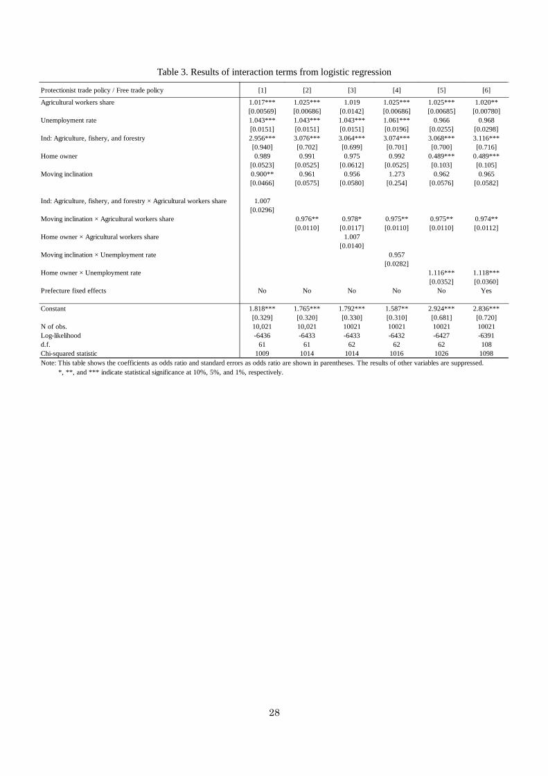
Table 3. Results of interaction terms from logistic regression
Protectionist trade policy / Free trade policy [1] [2] [3] [4] [5] [6]
Agricultural workers share 1.017*** 1.025*** 1.019 1.025*** 1.025*** 1.020**[0.00569] [0.00686] [0.0142] [0.00686] [0.00685] [0.00780]
Unemployment rate 1.043*** 1.043*** 1.043*** 1.061*** 0.966 0.968[0.0151] [0.0151] [0.0151] [0.0196] [0.0255] [0.0298]
Ind: Agriculture, fishery, and forestry 2.956*** 3.076*** 3.064*** 3.074*** 3.068*** 3.116***[0.940] [0.702] [0.699] [0.701] [0.700] [0.716]
Home owner 0.989 0.991 0.975 0.992 0.489*** 0.489***[0.0523] [0.0525] [0.0612] [0.0525] [0.103] [0.105]
Moving inclination 0.900** 0.961 0.956 1.273 0.962 0.965[0.0466] [0.0575] [0.0580] [0.254] [0.0576] [0.0582]
Ind: Agriculture, fishery, and forestry × Agricultural workers share 1.007[0.0296]
Moving inclination × Agricultural workers share 0.976** 0.978* 0.975** 0.975** 0.974**[0.0110] [0.0117] [0.0110] [0.0110] [0.0112]
Home owner × Agricultural workers share 1.007[0.0140]
Moving inclination × Unemployment rate 0.957[0.0282]
Home owner × Unemployment rate 1.116*** 1.118***[0.0352] [0.0360]
Prefecture fixed effects No No No No No Yes
Constant 1.818*** 1.765*** 1.792*** 1.587** 2.924*** 2.836***[0.329] [0.320] [0.330] [0.310] [0.681] [0.720]
N of obs. 10,021 10,021 10021 10021 10021 10021Log-likelihood -6436 -6433 -6433 -6432 -6427 -6391d.f. 61 61 62 62 62 108Chi-squared statistic 1009 1014 1014 1016 1026 1098Note: This table shows the coefficients as odds ratio and standard errors as odds ratio are shown in parentheses. The results of other variables are suppressed. *, **, and *** indicate statistical significance at 10%, 5%, and 1%, respectively.
28
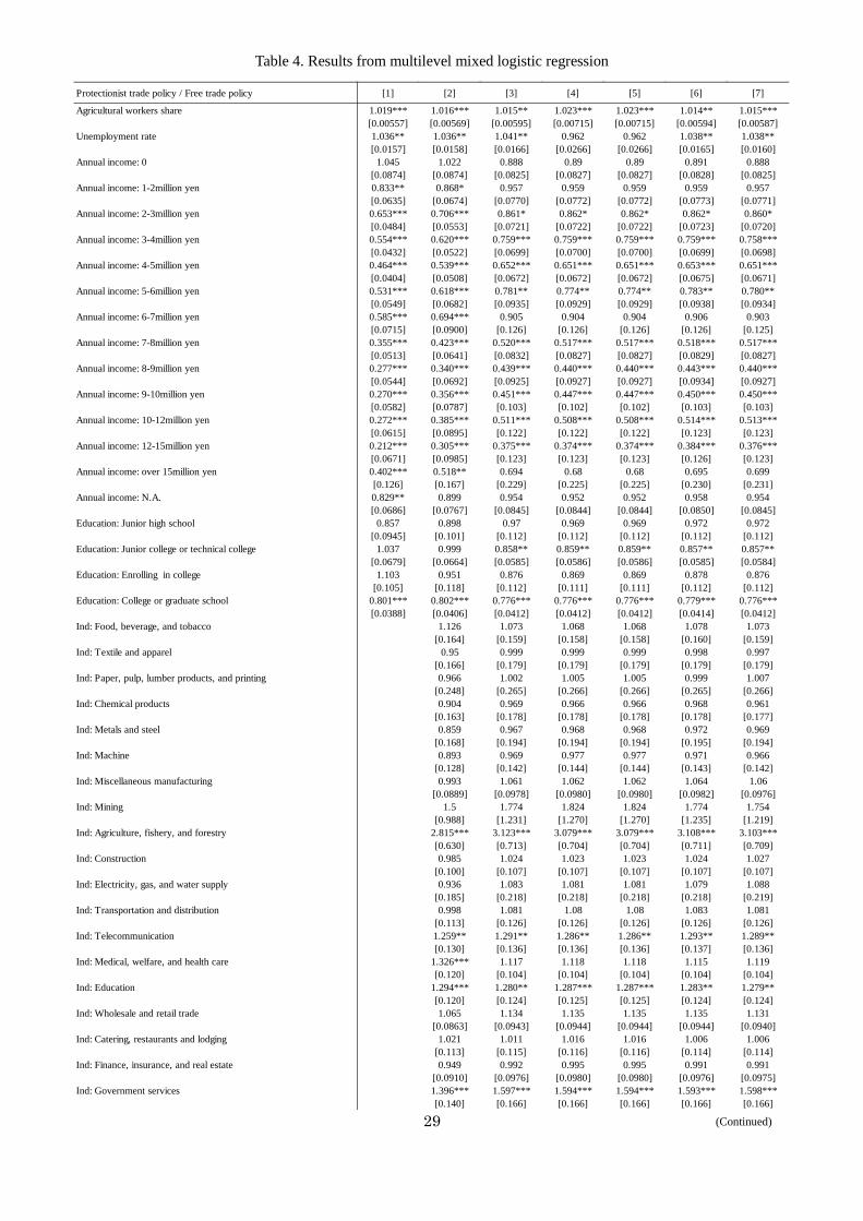
Table 4. Results from multilevel mixed logistic regression
Protectionist trade policy / Free trade policy [1] [2] [3] [4] [5] [6] [7]
Agricultural workers share 1.019*** 1.016*** 1.015** 1.023*** 1.023*** 1.014** 1.015***[0.00557] [0.00569] [0.00595] [0.00715] [0.00715] [0.00594] [0.00587]
Unemployment rate 1.036** 1.036** 1.041** 0.962 0.962 1.038** 1.038**[0.0157] [0.0158] [0.0166] [0.0266] [0.0266] [0.0165] [0.0160]
Annual income: 0 1.045 1.022 0.888 0.89 0.89 0.891 0.888[0.0874] [0.0874] [0.0825] [0.0827] [0.0827] [0.0828] [0.0825]
Annual income: 1-2million yen 0.833** 0.868* 0.957 0.959 0.959 0.959 0.957[0.0635] [0.0674] [0.0770] [0.0772] [0.0772] [0.0773] [0.0771]
Annual income: 2-3million yen 0.653*** 0.706*** 0.861* 0.862* 0.862* 0.862* 0.860*[0.0484] [0.0553] [0.0721] [0.0722] [0.0722] [0.0723] [0.0720]
Annual income: 3-4million yen 0.554*** 0.620*** 0.759*** 0.759*** 0.759*** 0.759*** 0.758***[0.0432] [0.0522] [0.0699] [0.0700] [0.0700] [0.0699] [0.0698]
Annual income: 4-5million yen 0.464*** 0.539*** 0.652*** 0.651*** 0.651*** 0.653*** 0.651***[0.0404] [0.0508] [0.0672] [0.0672] [0.0672] [0.0675] [0.0671]
Annual income: 5-6million yen 0.531*** 0.618*** 0.781** 0.774** 0.774** 0.783** 0.780**[0.0549] [0.0682] [0.0935] [0.0929] [0.0929] [0.0938] [0.0934]
Annual income: 6-7million yen 0.585*** 0.694*** 0.905 0.904 0.904 0.906 0.903[0.0715] [0.0900] [0.126] [0.126] [0.126] [0.126] [0.125]
Annual income: 7-8million yen 0.355*** 0.423*** 0.520*** 0.517*** 0.517*** 0.518*** 0.517***[0.0513] [0.0641] [0.0832] [0.0827] [0.0827] [0.0829] [0.0827]
Annual income: 8-9million yen 0.277*** 0.340*** 0.439*** 0.440*** 0.440*** 0.443*** 0.440***[0.0544] [0.0692] [0.0925] [0.0927] [0.0927] [0.0934] [0.0927]
Annual income: 9-10million yen 0.270*** 0.356*** 0.451*** 0.447*** 0.447*** 0.450*** 0.450***[0.0582] [0.0787] [0.103] [0.102] [0.102] [0.103] [0.103]
Annual income: 10-12million yen 0.272*** 0.385*** 0.511*** 0.508*** 0.508*** 0.514*** 0.513***[0.0615] [0.0895] [0.122] [0.122] [0.122] [0.123] [0.123]
Annual income: 12-15million yen 0.212*** 0.305*** 0.375*** 0.374*** 0.374*** 0.384*** 0.376***[0.0671] [0.0985] [0.123] [0.123] [0.123] [0.126] [0.123]
Annual income: over 15million yen 0.402*** 0.518** 0.694 0.68 0.68 0.695 0.699[0.126] [0.167] [0.229] [0.225] [0.225] [0.230] [0.231]
Annual income: N.A. 0.829** 0.899 0.954 0.952 0.952 0.958 0.954[0.0686] [0.0767] [0.0845] [0.0844] [0.0844] [0.0850] [0.0845]
Education: Junior high school 0.857 0.898 0.97 0.969 0.969 0.972 0.972[0.0945] [0.101] [0.112] [0.112] [0.112] [0.112] [0.112]
Education: Junior college or technical college 1.037 0.999 0.858** 0.859** 0.859** 0.857** 0.857**[0.0679] [0.0664] [0.0585] [0.0586] [0.0586] [0.0585] [0.0584]
Education: Enrolling in college 1.103 0.951 0.876 0.869 0.869 0.878 0.876[0.105] [0.118] [0.112] [0.111] [0.111] [0.112] [0.112]
Education: College or graduate school 0.801*** 0.802*** 0.776*** 0.776*** 0.776*** 0.779*** 0.776***[0.0388] [0.0406] [0.0412] [0.0412] [0.0412] [0.0414] [0.0412]
Ind: Food, beverage, and tobacco 1.126 1.073 1.068 1.068 1.078 1.073[0.164] [0.159] [0.158] [0.158] [0.160] [0.159]
Ind: Textile and apparel 0.95 0.999 0.999 0.999 0.998 0.997[0.166] [0.179] [0.179] [0.179] [0.179] [0.179]
Ind: Paper, pulp, lumber products, and printing 0.966 1.002 1.005 1.005 0.999 1.007[0.248] [0.265] [0.266] [0.266] [0.265] [0.266]
Ind: Chemical products 0.904 0.969 0.966 0.966 0.968 0.961[0.163] [0.178] [0.178] [0.178] [0.178] [0.177]
Ind: Metals and steel 0.859 0.967 0.968 0.968 0.972 0.969[0.168] [0.194] [0.194] [0.194] [0.195] [0.194]
Ind: Machine 0.893 0.969 0.977 0.977 0.971 0.966[0.128] [0.142] [0.144] [0.144] [0.143] [0.142]
Ind: Miscellaneous manufacturing 0.993 1.061 1.062 1.062 1.064 1.06[0.0889] [0.0978] [0.0980] [0.0980] [0.0982] [0.0976]
Ind: Mining 1.5 1.774 1.824 1.824 1.774 1.754[0.988] [1.231] [1.270] [1.270] [1.235] [1.219]
Ind: Agriculture, fishery, and forestry 2.815*** 3.123*** 3.079*** 3.079*** 3.108*** 3.103***[0.630] [0.713] [0.704] [0.704] [0.711] [0.709]
Ind: Construction 0.985 1.024 1.023 1.023 1.024 1.027[0.100] [0.107] [0.107] [0.107] [0.107] [0.107]
Ind: Electricity, gas, and water supply 0.936 1.083 1.081 1.081 1.079 1.088[0.185] [0.218] [0.218] [0.218] [0.218] [0.219]
Ind: Transportation and distribution 0.998 1.081 1.08 1.08 1.083 1.081[0.113] [0.126] [0.126] [0.126] [0.126] [0.126]
Ind: Telecommunication 1.259** 1.291** 1.286** 1.286** 1.293** 1.289**[0.130] [0.136] [0.136] [0.136] [0.137] [0.136]
Ind: Medical, welfare, and health care 1.326*** 1.117 1.118 1.118 1.115 1.119[0.120] [0.104] [0.104] [0.104] [0.104] [0.104]
Ind: Education 1.294*** 1.280** 1.287*** 1.287*** 1.283** 1.279**[0.120] [0.124] [0.125] [0.125] [0.124] [0.124]
Ind: Wholesale and retail trade 1.065 1.134 1.135 1.135 1.135 1.131[0.0863] [0.0943] [0.0944] [0.0944] [0.0944] [0.0940]
Ind: Catering, restaurants and lodging 1.021 1.011 1.016 1.016 1.006 1.006[0.113] [0.115] [0.116] [0.116] [0.114] [0.114]
Ind: Finance, insurance, and real estate 0.949 0.992 0.995 0.995 0.991 0.991[0.0910] [0.0976] [0.0980] [0.0980] [0.0976] [0.0975]
Ind: Government services 1.396*** 1.597*** 1.594*** 1.594*** 1.593*** 1.598***[0.140] [0.166] [0.166] [0.166] [0.166] [0.166]
(Continued) 29
Protectionist trade policy / Free trade policy [1] [2] [3] [4] [5] [6] [7]
(cont.)
Occupation: Production and other operations 0.830* 0.923 0.918 0.918 0.92 0.921[0.0796] [0.0914] [0.0910] [0.0910] [0.0913] [0.0911]
Occupation: Managerial occupation 0.502*** 0.715*** 0.712*** 0.712*** 0.713*** 0.716***[0.0391] [0.0591] [0.0589] [0.0589] [0.0590] [0.0591]
Occupation: Professional or technical occupation 0.748*** 0.894* 0.892* 0.892* 0.891* 0.891*[0.0442] [0.0552] [0.0552] [0.0552] [0.0552] [0.0550]
Occupation: Other occupations 0.773*** 0.893 0.897 0.897 0.892 0.892[0.0528] [0.0631] [0.0634] [0.0634] [0.0631] [0.0630]
Occupation: Never worked or in school 0.987 1.09 1.098 1.098 1.082 1.086[0.193] [0.222] [0.224] [0.224] [0.221] [0.221]
Emp type: Officer or executive 0.836** 0.938 0.939 0.939 0.938 0.937[0.0756] [0.0873] [0.0874] [0.0874] [0.0873] [0.0872]
Emp type: Non-regular employee 0.974 0.921 0.918 0.918 0.922 0.92[0.0553] [0.0547] [0.0546] [0.0546] [0.0549] [0.0546]
Emp type: Self-employment or profession 0.854** 0.947 0.942 0.942 0.947 0.946[0.0571] [0.0666] [0.0664] [0.0664] [0.0667] [0.0666]
Emp type: In school or no experience to work 1.207 0.912 0.9 0.9 0.919 0.915[0.232] [0.182] [0.180] [0.180] [0.184] [0.183]
Gender: Female=1 1.692*** 1.692*** 1.692*** 1.698*** 1.691***[0.0945] [0.0946] [0.0946] [0.0950] [0.0944]
Age 0.978*** 0.978*** 0.978*** 0.978*** 0.978***[0.00202] [0.00202] [0.00202] [0.00202] [0.00202]
Currently employed 1.065 1.064 1.064 1.067 1.065[0.0659] [0.0659] [0.0659] [0.0661] [0.0659]
Having a child 0.894** 0.894** 0.894** 0.895** 0.895**[0.0476] [0.0477] [0.0477] [0.0477] [0.0476]
Patriot 1.251*** 1.251*** 1.251*** 1.249*** 1.248***[0.0559] [0.0559] [0.0559] [0.0559] [0.0558]
Disaster victim 0.931 0.934 0.934 0.922 0.932[0.0803] [0.0807] [0.0807] [0.0790] [0.0794]
Food checker 1.274*** 1.271*** 1.271*** 1.273*** 1.272***[0.0615] [0.0614] [0.0614] [0.0616] [0.0614]
Risk averter 1.373*** 1.374*** 1.374*** 1.371*** 1.373***[0.0645] [0.0646] [0.0646] [0.0645] [0.0645]
Optimist 0.743*** 0.742*** 0.742*** 0.743*** 0.743***[0.0472] [0.0472] [0.0472] [0.0472] [0.0472]
Home owner 0.993 0.485*** 0.485*** 0.989 0.999[0.0529] [0.102] [0.102] [0.0527] [0.0575]
Moving inclination 0.901** 0.963 0.963 0.883** 0.902**[0.0467] [0.0578] [0.0578] [0.0526] [0.0468]
Job change inclination 0.908* 0.908* 0.908* 0.907* 0.907*[0.0471] [0.0472] [0.0472] [0.0471] [0.0470]
Moving inclination × Agricultural workers share 0.975** 0.975**[0.0111] [0.0111]
Home owner × Unemployment rate 1.118*** 1.118***[0.0354] [0.0354]
Constant 1.099 1.229 1.845*** 3.018*** 3.018*** 1.907*** 1.881***[0.128] [0.166] [0.348] [0.726] [0.726] [0.363] [0.348]
Random intercept at the prefecture level 0.0915*** 0.0888*** 0.105*** 0.106*** 0.106*** 0.154*** 0.113***[0.0337] [0.0350] [0.0342] [0.0339] [0.0339] [0.0561] [0.0343]
Random intercept at the city level 3.76E-08[0.0814]
Random coefficient ([6]: Moving inclination, [7]: Home owner 0.149*** 0.118***[0.0390] [0.0384]
N of obs. 10,021 10,021 10,021 10,021 10,021 10,021 10,021N of groups 47 47 47 47 47 47 47Log-likelihood -6733 -6647 -6433 -6424 -6424 -6430 -6433d.f. 20 48 60 62 62 60 60Chi-squared statistic 376.4 520.6 872.7 884.5 884.5 866 867Note: This table shows the coefficients as odds ratio and standard errors as odds ratio are shown in parentheses. *, **, and *** indicate statistical significance at 10%, 5%, and 1%, respectively.
30
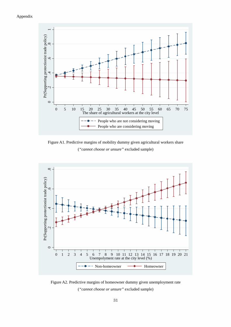
Appendix
Figure A1. Predictive margins of mobility dummy given agricultural workers share
(“cannot choose or unsure” excluded sample)
Figure A2. Predictive margins of homeowner dummy given unemployment rate
(“cannot choose or unsure” excluded sample)
0.2
.4.6
.81
Pr(S
uppo
rting
pro
tect
ioni
st tr
ade
polic
y)
0 5 10 15 20 25 30 35 40 45 50 55 60 65 70 75The share of agricultural workers at the city level
People who are not considering movingPeople who are considering moving
0.2
.4.6
.8Pr
(Sup
porti
ng p
rote
ctio
nist
trad
e po
licy)
0 1 2 3 4 5 6 7 8 9 10 11 12 13 14 15 16 17 18 19 20 21Unempolyment rate at the city level (%)
Non-homeowner Homeowner
31

Figure A3. Unobserved heterogeneity in trade policy preferences across prefectures
(“cannot choose or unsure” excluded sample)
Note: Random intercepts by prefectures are shown. Positive coefficients on the right-hand side indicate an increase in the probability of
supporting a protectionist trade policy whereas negative coefficients on the left-hand side indicate an increase in the probability of supporting
a free trade policy.
-0.3 -0.2 -0.1 0 0.1 0.2 0.3 0.4
HokkaidoAomori
IwateMiyagi
AkitaYamagata
FukushimaIbaraki
TochigiGunma
SaitamaChibaTokyo
KanagawaNiigata
ToyamaIshikawa
FukuiYamanashi
NaganoGifu
ShizuokaAichi
MieShigaKyotoOsakaHyogo
NaraWakayama
TottoriShimane
OkayamaHiroshima
YamaguchiTokushima
KagawaEhimeKochi
FukuokaSaga
NagasakiKumamoto
OitaMiyazaki
KagoshimaOkinawa
32
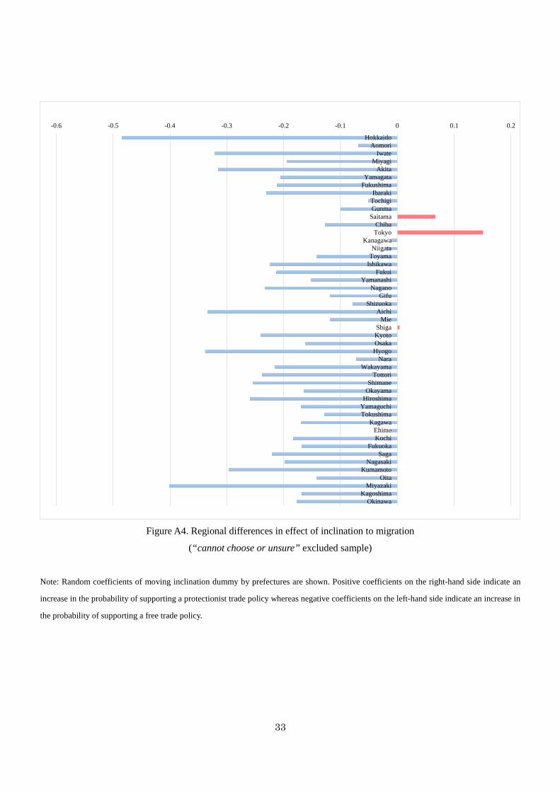
Figure A4. Regional differences in effect of inclination to migration
(“cannot choose or unsure” excluded sample)
Note: Random coefficients of moving inclination dummy by prefectures are shown. Positive coefficients on the right-hand side indicate an
increase in the probability of supporting a protectionist trade policy whereas negative coefficients on the left-hand side indicate an increase in
the probability of supporting a free trade policy.
-0.6 -0.5 -0.4 -0.3 -0.2 -0.1 0 0.1 0.2
HokkaidoAomori
IwateMiyagi
AkitaYamagata
FukushimaIbaraki
TochigiGunma
SaitamaChibaTokyo
KanagawaNiigata
ToyamaIshikawa
FukuiYamanashi
NaganoGifu
ShizuokaAichi
MieShigaKyotoOsakaHyogo
NaraWakayama
TottoriShimane
OkayamaHiroshima
YamaguchiTokushima
KagawaEhimeKochi
FukuokaSaga
NagasakiKumamoto
OitaMiyazaki
KagoshimaOkinawa
33

Figure A5. Regional differences in home ownership effect
(“cannot choose or unsure” excluded sample)
Note: Random coefficients of home ownership dummy by prefectures are shown. Positive coefficients on the right-hand side indicate an
increase in the probability of supporting a protectionist trade policy whereas negative coefficients on the left-hand side indicate an increase in
the probability of supporting a free trade policy.
-0.4 -0.3 -0.2 -0.1 0 0.1 0.2 0.3
HokkaidoAomori
IwateMiyagi
AkitaYamagata
FukushimaIbaraki
TochigiGunma
SaitamaChibaTokyo
KanagawaNiigata
ToyamaIshikawa
FukuiYamanashi
NaganoGifu
ShizuokaAichi
MieShigaKyotoOsakaHyogo
NaraWakayama
TottoriShimane
OkayamaHiroshima
YamaguchiTokushima
KagawaEhimeKochi
FukuokaSaga
NagasakiKumamoto
OitaMiyazaki
KagoshimaOkinawa
34
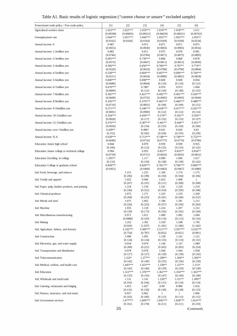
Table A1. Basic results of logistic regression (“cannot choose or unsure” excluded sample)
Protectionist trade policy / Free trade policy [1] [2] [3] [4] [5] [6]
Agricultural workers share 1.023*** 1.022*** 1.019*** 1.019*** 1.018*** 1.011[0.00596] [0.00605] [0.00612] [0.00629] [0.00631] [0.00762]
Unemployment rate 1.044*** 1.051*** 1.044*** 1.052*** 1.052*** 1.055**[0.0162] [0.0164] [0.0164] [0.0169] [0.0169] [0.0234]
Annual income: 0 0.987 0.972 0.871 0.871 0.875[0.0925] [0.0930] [0.0903] [0.0905] [0.0916]
Annual income: 1-2million yen 0.882 0.911 0.975 0.978 0.991[0.0746] [0.0784] [0.0871] [0.0875] [0.0895]
Annual income: 2-3million yen 0.695*** 0.739*** 0.868 0.868 0.878[0.0575] [0.0647] [0.0811] [0.0813] [0.0830]
Annual income: 3-4million yen 0.596*** 0.656*** 0.766*** 0.767** 0.774**[0.0520] [0.0619] [0.0788] [0.0790] [0.0804]
Annual income: 4-5million yen 0.528*** 0.604*** 0.697*** 0.696*** 0.704***[0.0511] [0.0634] [0.0800] [0.0801] [0.0818]
Annual income: 5-6million yen 0.600*** 0.690*** 0.828 0.828 0.834[0.0686] [0.0844] [0.110] [0.110] [0.112]
Annual income: 6-7million yen 0.670*** 0.786* 0.976 0.973 1.004[0.0899] [0.112] [0.150] [0.149] [0.155]
Annual income: 7-8million yen 0.365*** 0.421*** 0.492*** 0.491*** 0.505***[0.0608] [0.0735] [0.0905] [0.0905] [0.0940]
Annual income: 8-9million yen 0.326*** 0.379*** 0.465*** 0.466*** 0.488***[0.0710] [0.0855] [0.109] [0.109] [0.115]
Annual income: 9-10million yen 0.271*** 0.346*** 0.418*** 0.417*** 0.421***[0.0691] [0.0900] [0.112] [0.112] [0.114]
Annual income: 10-12million yen 0.334*** 0.459*** 0.579** 0.581** 0.593**[0.0828] [0.117] [0.152] [0.153] [0.157]
Annual income: 12-15million yen 0.276*** 0.387*** 0.441** 0.444** 0.451**[0.0936] [0.134] [0.155] [0.156] [0.160]
Annual income: over 15million yen 0.428** 0.496* 0.631 0.626 0.63[0.152] [0.182] [0.236] [0.235] [0.239]
Annual income: N.A. 0.658*** 0.713*** 0.748*** 0.749*** 0.752***[0.0640] [0.0716] [0.0775] [0.0776] [0.0786]
Education: Junior high school 0.844 0.879 0.939 0.939 0.925[0.106] [0.112] [0.122] [0.123] [0.122]
Education: Junior college or technical college 0.994 0.955 0.831** 0.832** 0.834**[0.0739] [0.0721] [0.0643] [0.0645] [0.0652]
Education: Enrolling in college 1.295** 1.117 0.999 1.006 1.017[0.133] [0.150] [0.138] [0.139] [0.142]
Education: College or graduate school 0.838*** 0.829*** 0.781*** 0.786*** 0.800***[0.0455] [0.0469] [0.0463] [0.0467] [0.0480]
Ind: Food, beverage, and tobacco 1.213 1.225 1.169 1.174 1.175[0.196] [0.199] [0.193] [0.194] [0.196]
Ind: Textile and apparel 1.032 0.946 1.023 1.008 1[0.207] [0.191] [0.211] [0.208] [0.208]
Ind: Paper, pulp, lumber products, and printing 1.218 1.159 1.241 1.229 1.219[0.336] [0.321] [0.354] [0.350] [0.348]
Ind: Chemical products 1.073 1.171 1.225 1.219 1.269[0.204] [0.225] [0.241] [0.240] [0.252]
Ind: Metals and steel 1.075 1.062 1.186 1.181 1.212[0.226] [0.225] [0.257] [0.256] [0.264]
Ind: Machine 1.035 1.118 1.214 1.207 1.212[0.159] [0.173] [0.193] [0.192] [0.194]
Ind: Miscellaneous manufacturing 0.971 1.011 1.089 1.082 1.094[0.0980] [0.103] [0.114] [0.113] [0.116]
Ind: Mining 1.252 1.391 1.539 1.548 1.745[0.926] [1.037] [1.181] [1.186] [1.342]
Ind: Agriculture, fishery, and forestry 3.192*** 3.300*** 3.511*** 3.507*** 3.632***[0.754] [0.787] [0.852] [0.851] [0.891]
Ind: Construction 1.096 1.091 1.138 1.141 1.121[0.124] [0.124] [0.133] [0.133] [0.132]
Ind: Electricity, gas, and water supply 0.918 0.974 1.146 1.147 1.089[0.206] [0.221] [0.265] [0.265] [0.254]
Ind: Transportation and distribution 0.978 0.978 1.046 1.044 1.058[0.127] [0.127] [0.139] [0.139] [0.142]
Ind: Telecommunication 1.222* 1.277** 1.299** 1.304** 1.305**[0.142] [0.149] [0.155] [0.156] [0.158]
Ind: Medical, welfare, and health care 1.445*** 1.423*** 1.239** 1.237** 1.215*[0.145] [0.144] [0.129] [0.129] [0.128]
Ind: Education 1.312*** 1.376*** 1.361*** 1.354*** 1.363***[0.133] [0.143] [0.147] [0.146] [0.148]
Ind: Wholesale and retail trade 1.131 1.141 1.226** 1.221** 1.206**[0.103] [0.104] [0.115] [0.114] [0.114]
Ind: Catering, restaurants and lodging 1.053 1.027 0.99 0.988 1.016[0.133] [0.130] [0.128] [0.128] [0.133]
Ind: Finance, insurance, and real estate 0.937 0.962 1 1 1.006[0.103] [0.106] [0.113] [0.113] [0.115]
Ind: Government services 1.477*** 1.609*** 1.845*** 1.838*** 1.814***[0.161] [0.178] [0.211] [0.211] [0.210]
(Continued) 35
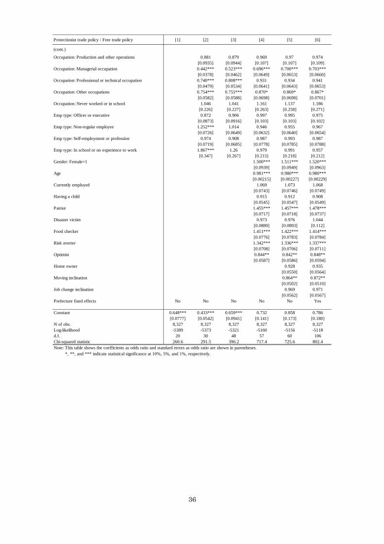
Protectionist trade policy / Free trade policy [1] [2] [3] [4] [5] [6]
(cont.)
Occupation: Production and other operations 0.881 0.879 0.969 0.97 0.974[0.0935] [0.0944] [0.107] [0.107] [0.109]
Occupation: Managerial occupation 0.442*** 0.523*** 0.696*** 0.700*** 0.703***[0.0378] [0.0462] [0.0649] [0.0653] [0.0660]
Occupation: Professional or technical occupation 0.740*** 0.808*** 0.931 0.934 0.941[0.0479] [0.0534] [0.0641] [0.0643] [0.0653]
Occupation: Other occupations 0.754*** 0.755*** 0.870* 0.869* 0.867*[0.0582] [0.0588] [0.0698] [0.0698] [0.0701]
Occupation: Never worked or in school 1.046 1.041 1.161 1.137 1.186[0.226] [0.227] [0.263] [0.258] [0.271]
Emp type: Officer or executive 0.872 0.906 0.997 0.995 0.975[0.0873] [0.0916] [0.103] [0.103] [0.102]
Emp type: Non-regular employee 1.252*** 1.014 0.946 0.955 0.967[0.0726] [0.0649] [0.0632] [0.0640] [0.0654]
Emp type: Self-employment or profession 0.974 0.908 0.987 0.993 0.987[0.0719] [0.0685] [0.0778] [0.0785] [0.0788]
Emp type: In school or no experience to work 1.867*** 1.26 0.979 0.991 0.957[0.347] [0.267] [0.215] [0.218] [0.212]
Gender: Female=1 1.500*** 1.511*** 1.520***[0.0939] [0.0949] [0.0963]
Age 0.981*** 0.980*** 0.980***[0.00215] [0.00227] [0.00229]
Currently employed 1.069 1.073 1.068[0.0743] [0.0746] [0.0749]
Having a child 0.915 0.912 0.908[0.0545] [0.0547] [0.0549]
Patriot 1.455*** 1.457*** 1.478***[0.0717] [0.0718] [0.0737]
Disaster victim 0.973 0.976 1.044[0.0889] [0.0893] [0.112]
Food checker 1.411*** 1.422*** 1.414***[0.0776] [0.0783] [0.0784]
Risk averter 1.342*** 1.336*** 1.337***[0.0708] [0.0706] [0.0711]
Optimist 0.844** 0.842** 0.848**[0.0587] [0.0586] [0.0594]
Home owner 0.928 0.935[0.0550] [0.0564]
Moving inclination 0.864** 0.872**[0.0502] [0.0510]
Job change inclination 0.969 0.971[0.0562] [0.0567]
Prefecture fixed effects No No No No No Yes
Constant 0.648*** 0.433*** 0.659*** 0.732 0.858 0.786[0.0777] [0.0542] [0.0941] [0.141] [0.173] [0.180]
N of obs. 8,327 8,327 8,327 8,327 8,327 8,327Log-likelihood -5389 -5373 -5321 -5160 -5156 -5118d.f. 20 30 48 57 60 106Chi-squared statistic 260.6 291.5 396.2 717.4 725.6 802.4Note: This table shows the coefficients as odds ratio and standard errors as odds ratio are shown in parentheses. *, **, and *** indicate statistical significance at 10%, 5%, and 1%, respectively.
36
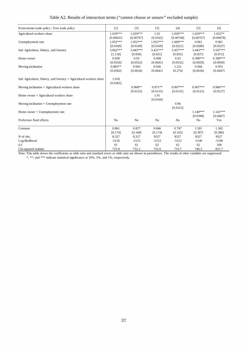
Table A2. Results of interaction terms (“cannot choose or unsure” excluded sample)
Protectionist trade policy / Free trade policy [1] [2] [3] [4] [5] [6]
Agricultural workers share 1.018*** 1.029*** 1.02 1.030*** 1.029*** 1.022**[0.00641] [0.00767] [0.0162] [0.00768] [0.00767] [0.00878]
Unemployment rate 1.052*** 1.052*** 1.052*** 1.069*** 0.961 0.961[0.0169] [0.0169] [0.0169] [0.0221] [0.0280] [0.0327]
Ind: Agriculture, fishery, and forestry 3.062*** 3.443*** 3.421*** 3.437*** 3.443*** 3.547***[1.118] [0.836] [0.831] [0.835] [0.837] [0.872]
Home owner 0.928 0.93 0.908 0.93 0.398*** 0.399***[0.0550] [0.0552] [0.0641] [0.0552] [0.0929] [0.0950]
Moving inclination 0.865** 0.943 0.936 1.231 0.944 0.953[0.0502] [0.0634] [0.0641] [0.274] [0.0636] [0.0647]
Ind: Agriculture, fishery, and forestry × Agricultural workers share 1.018[0.0365]
Moving inclination × Agricultural workers share 0.968** 0.971** 0.967*** 0.967*** 0.966***[0.0125] [0.0135] [0.0125] [0.0125] [0.0127]
Home owner × Agricultural workers share 1.01[0.0160]
Moving inclination × Unemployment rate 0.96[0.0315]
Home owner × Unemployment rate 1.140*** 1.141***[0.0398] [0.0407]
Prefecture fixed effects No No No No No Yes
Constant 0.861 0.827 0.846 0.747 1.501 1.365[0.174] [0.168] [0.174] [0.163] [0.387] [0.386]
N of obs. 8,327 8,327 8327 8327 8327 8327Log-likelihood -5156 -5153 -5153 -5152 -5146 -5108d.f. 61 61 62 62 62 108Chi-squared statistic 725.8 732.2 732.6 733.7 746.5 822.7Note: This table shows the coefficients as odds ratio and standard errors as odds ratio are shown in parentheses. The results of other variables are suppressed. *, **, and *** indicate statistical significance at 10%, 5%, and 1%, respectively.
37
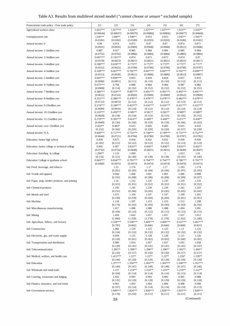
Table A3. Results from multilevel mixed model (“cannot choose or unsure” excluded sample)
Protectionist trade policy / Free trade policy [1] [2] [3] [4] [5] [6] [7]
Agricultural workers share 1.021*** 1.017*** 1.016** 1.027*** 1.027*** 1.015** 1.016**[0.00644] [0.00657] [0.00679] [0.00806] [0.00806] [0.00677] [0.00668]
Unemployment rate 1.041** 1.040** 1.046** 0.953 0.953 1.045** 1.042**[0.0181] [0.0182] [0.0189] [0.0293] [0.0293] [0.0186] [0.0181]
Annual income: 0 0.99 0.974 0.872 0.87 0.87 0.874 0.871[0.0931] [0.0935] [0.0909] [0.0908] [0.0908] [0.0912] [0.0908]
Annual income: 1-2million yen 0.887 0.917 0.985 0.984 0.984 0.985 0.984[0.0752] [0.0792] [0.0884] [0.0884] [0.0884] [0.0885] [0.0884]
Annual income: 2-3million yen 0.697*** 0.743*** 0.874 0.873 0.873 0.874 0.87[0.0578] [0.0653] [0.0821] [0.0821] [0.0821] [0.0822] [0.0817]
Annual income: 3-4million yen 0.598*** 0.659*** 0.773** 0.772** 0.772** 0.772** 0.771**[0.0522] [0.0623] [0.0799] [0.0799] [0.0799] [0.0799] [0.0797]
Annual income: 4-5million yen 0.528*** 0.607*** 0.702*** 0.697*** 0.697*** 0.702*** 0.699***[0.0513] [0.0639] [0.0811] [0.0806] [0.0806] [0.0813] [0.0807]
Annual income: 5-6million yen 0.602*** 0.694*** 0.835 0.824 0.824 0.837 0.833[0.0690] [0.0851] [0.111] [0.110] [0.110] [0.112] [0.111]
Annual income: 6-7million yen 0.675*** 0.794 0.989 0.984 0.984 0.987 0.982[0.0908] [0.114] [0.152] [0.152] [0.152] [0.152] [0.151]
Annual income: 7-8million yen 0.366*** 0.424*** 0.497*** 0.491*** 0.491*** 0.492*** 0.491***[0.0612] [0.0743] [0.0920] [0.0909] [0.0909] [0.0912] [0.0909]
Annual income: 8-9million yen 0.331*** 0.386*** 0.478*** 0.478*** 0.478*** 0.482*** 0.478***[0.0722] [0.0872] [0.112] [0.112] [0.112] [0.113] [0.112]
Annual income: 9-10million yen 0.274*** 0.349*** 0.423*** 0.416*** 0.416*** 0.421*** 0.422***[0.0699] [0.0910] [0.114] [0.112] [0.112] [0.114] [0.114]
Annual income: 10-12million yen 0.333*** 0.459*** 0.585** 0.581** 0.581** 0.589** 0.589**[0.0828] [0.118] [0.154] [0.153] [0.153] [0.156] [0.155]
Annual income: 12-15million yen 0.279*** 0.393*** 0.453** 0.449** 0.449** 0.471** 0.458**[0.0949] [0.136] [0.160] [0.159] [0.159] [0.166] [0.162]
Annual income: over 15million yen 0.424** 0.493* 0.623 0.605 0.605 0.625 0.632[0.152] [0.182] [0.235] [0.229] [0.229] [0.237] [0.239]
Annual income: N.A. 0.660*** 0.717*** 0.753*** 0.749*** 0.749*** 0.755*** 0.752***[0.0644] [0.0721] [0.0784] [0.0780] [0.0780] [0.0787] [0.0782]
Education: Junior high school 0.839 0.875 0.934 0.932 0.932 0.939 0.939[0.105] [0.112] [0.122] [0.122] [0.122] [0.123] [0.123]
Education: Junior college or technical college 0.995 0.957 0.833** 0.836** 0.836** 0.833** 0.832**[0.0742] [0.0724] [0.0648] [0.0651] [0.0651] [0.0649] [0.0647]
Education: Enrolling in college 1.296** 1.119 1.009 1 1 1.013 1.01[0.133] [0.151] [0.140] [0.139] [0.139] [0.141] [0.140]
Education: College or graduate school 0.843*** 0.834*** 0.793*** 0.794*** 0.794*** 0.796*** 0.792***[0.0460] [0.0475] [0.0473] [0.0474] [0.0474] [0.0476] [0.0473]
Ind: Food, beverage, and tobacco 1.23 1.176 1.17 1.17 1.183 1.174[0.201] [0.195] [0.194] [0.194] [0.197] [0.195]
Ind: Textile and apparel 0.944 1.006 1.001 1.001 1.006 0.998[0.191] [0.208] [0.208] [0.208] [0.209] [0.207]
Ind: Paper, pulp, lumber products, and printing 1.16 1.232 1.235 1.235 1.229 1.235[0.321] [0.351] [0.352] [0.352] [0.351] [0.352]
Ind: Chemical products 1.195 1.245 1.239 1.239 1.241 1.225[0.231] [0.246] [0.245] [0.245] [0.245] [0.242]
Ind: Metals and steel 1.075 1.194 1.197 1.197 1.199 1.201[0.228] [0.259] [0.260] [0.260] [0.261] [0.261]
Ind: Machine 1.118 1.207 1.223 1.223 1.212 1.208[0.174] [0.192] [0.195] [0.195] [0.193] [0.192]
Ind: Miscellaneous manufacturing 1.017 1.088 1.088 1.088 1.094 1.091[0.104] [0.114] [0.115] [0.115] [0.115] [0.115]
Ind: Mining 1.458 1.643 1.657 1.657 1.637 1.612[1.090] [1.259] [1.278] [1.278] [1.262] [1.240]
Ind: Agriculture, fishery, and forestry 3.328*** 3.538*** 3.469*** 3.469*** 3.522*** 3.491***[0.795] [0.862] [0.846] [0.846] [0.860] [0.851]
Ind: Construction 1.082 1.129 1.125 1.125 1.13 1.131[0.124] [0.132] [0.132] [0.132] [0.132] [0.132]
Ind: Electricity, gas, and water supply 0.958 1.125 1.128 1.128 1.121 1.126[0.218] [0.261] [0.262] [0.262] [0.260] [0.261]
Ind: Transportation and distribution 0.986 1.054 1.057 1.057 1.055 1.058[0.129] [0.141] [0.141] [0.141] [0.141] [0.141]
Ind: Telecommunication 1.281** 1.308** 1.296** 1.296** 1.302** 1.304**[0.150] [0.157] [0.156] [0.156] [0.157] [0.157]
Ind: Medical, welfare, and health care 1.415*** 1.227* 1.227* 1.227* 1.226* 1.228**[0.144] [0.128] [0.129] [0.129] [0.128] [0.128]
Ind: Education 1.377*** 1.354*** 1.363*** 1.363*** 1.358*** 1.351***[0.144] [0.147] [0.148] [0.148] [0.147] [0.146]
Ind: Wholesale and retail trade 1.137 1.214** 1.216** 1.216** 1.219** 1.212**[0.104] [0.114] [0.114] [0.114] [0.115] [0.114]
Ind: Catering, restaurants and lodging 1.032 0.993 0.993 0.993 0.991 0.988[0.131] [0.129] [0.129] [0.129] [0.129] [0.128]
Ind: Finance, insurance, and real estate 0.963 1.003 1.004 1.004 0.998 0.998[0.107] [0.114] [0.114] [0.114] [0.114] [0.113]
Ind: Government services 1.600*** 1.824*** 1.826*** 1.826*** 1.825*** 1.828***[0.178] [0.210] [0.211] [0.211] [0.211] [0.211]
(Continued) 38
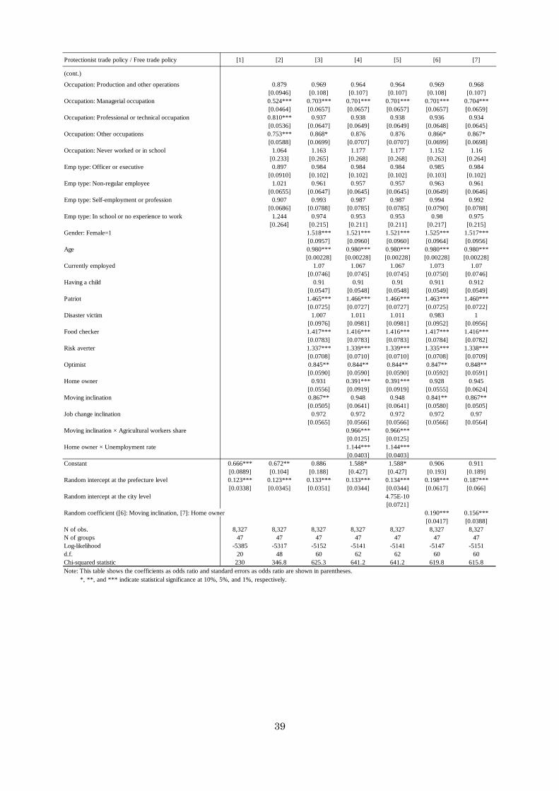
Protectionist trade policy / Free trade policy [1] [2] [3] [4] [5] [6] [7]
(cont.)
Occupation: Production and other operations 0.879 0.969 0.964 0.964 0.969 0.968[0.0946] [0.108] [0.107] [0.107] [0.108] [0.107]
Occupation: Managerial occupation 0.524*** 0.703*** 0.701*** 0.701*** 0.701*** 0.704***[0.0464] [0.0657] [0.0657] [0.0657] [0.0657] [0.0659]
Occupation: Professional or technical occupation 0.810*** 0.937 0.938 0.938 0.936 0.934[0.0536] [0.0647] [0.0649] [0.0649] [0.0648] [0.0645]
Occupation: Other occupations 0.753*** 0.868* 0.876 0.876 0.866* 0.867*[0.0588] [0.0699] [0.0707] [0.0707] [0.0699] [0.0698]
Occupation: Never worked or in school 1.064 1.163 1.177 1.177 1.152 1.16[0.233] [0.265] [0.268] [0.268] [0.263] [0.264]
Emp type: Officer or executive 0.897 0.984 0.984 0.984 0.985 0.984[0.0910] [0.102] [0.102] [0.102] [0.103] [0.102]
Emp type: Non-regular employee 1.021 0.961 0.957 0.957 0.963 0.961[0.0655] [0.0647] [0.0645] [0.0645] [0.0649] [0.0646]
Emp type: Self-employment or profession 0.907 0.993 0.987 0.987 0.994 0.992[0.0686] [0.0788] [0.0785] [0.0785] [0.0790] [0.0788]
Emp type: In school or no experience to work 1.244 0.974 0.953 0.953 0.98 0.975[0.264] [0.215] [0.211] [0.211] [0.217] [0.215]
Gender: Female=1 1.518*** 1.521*** 1.521*** 1.525*** 1.517***[0.0957] [0.0960] [0.0960] [0.0964] [0.0956]
Age 0.980*** 0.980*** 0.980*** 0.980*** 0.980***[0.00228] [0.00228] [0.00228] [0.00228] [0.00228]
Currently employed 1.07 1.067 1.067 1.073 1.07[0.0746] [0.0745] [0.0745] [0.0750] [0.0746]
Having a child 0.91 0.91 0.91 0.911 0.912[0.0547] [0.0548] [0.0548] [0.0549] [0.0549]
Patriot 1.465*** 1.466*** 1.466*** 1.463*** 1.460***[0.0725] [0.0727] [0.0727] [0.0725] [0.0722]
Disaster victim 1.007 1.011 1.011 0.983 1[0.0976] [0.0981] [0.0981] [0.0952] [0.0956]
Food checker 1.417*** 1.416*** 1.416*** 1.417*** 1.416***[0.0783] [0.0783] [0.0783] [0.0784] [0.0782]
Risk averter 1.337*** 1.339*** 1.339*** 1.335*** 1.338***[0.0708] [0.0710] [0.0710] [0.0708] [0.0709]
Optimist 0.845** 0.844** 0.844** 0.847** 0.848**[0.0590] [0.0590] [0.0590] [0.0592] [0.0591]
Home owner 0.931 0.391*** 0.391*** 0.928 0.945[0.0556] [0.0919] [0.0919] [0.0555] [0.0624]
Moving inclination 0.867** 0.948 0.948 0.841** 0.867**[0.0505] [0.0641] [0.0641] [0.0580] [0.0505]
Job change inclination 0.972 0.972 0.972 0.972 0.97[0.0565] [0.0566] [0.0566] [0.0566] [0.0564]
Moving inclination × Agricultural workers share 0.966*** 0.966***[0.0125] [0.0125]
Home owner × Unemployment rate 1.144*** 1.144***[0.0403] [0.0403]
Constant 0.666*** 0.672** 0.886 1.588* 1.588* 0.906 0.911[0.0889] [0.104] [0.188] [0.427] [0.427] [0.193] [0.189]
Random intercept at the prefecture level 0.123*** 0.123*** 0.133*** 0.133*** 0.134*** 0.198*** 0.187***[0.0338] [0.0345] [0.0351] [0.0344] [0.0344] [0.0617] [0.066]
Random intercept at the city level 4.75E-10[0.0721]
Random coefficient ([6]: Moving inclination, [7]: Home owner 0.190*** 0.156***[0.0417] [0.0388]
N of obs. 8,327 8,327 8,327 8,327 8,327 8,327 8,327N of groups 47 47 47 47 47 47 47Log-likelihood -5385 -5317 -5152 -5141 -5141 -5147 -5151d.f. 20 48 60 62 62 60 60Chi-squared statistic 230 346.8 625.3 641.2 641.2 619.8 615.8Note: This table shows the coefficients as odds ratio and standard errors as odds ratio are shown in parentheses. *, **, and *** indicate statistical significance at 10%, 5%, and 1%, respectively.
39