ISSN 0111-1760

University of OtagoEconomics Discussion Papers

No. 0608

21 December 2006

Trade Policy and Public Ownership

Ngo Van Long'

Frank Stahler

Correspondence to:Frank StahlerDepartment of EconomicsUniversity of OtagoPO Box 56, DunedinNew ZealandPhone: (64) 3 4798645Fax: (64) 3 4798174Email: fstaehler@business.otago.ac.nz

Corresponding author, Department of Economics, McGill University, Montreal, H3A 2TY, Canada,email: ngo.long@mcgill.ca

Abstract

This paper discusses the influence of public ownership on trade policy instru-ments. We demonstrate three important invariance results. First, the degreeof public ownership affects neither the level of socially optimal activities norwelfare if the government chooses optimal trade policy instruments. Second,in the case of rivalry between domestic export firms, the optimal exporttax is independent of the degree of public ownership. Third, in the case ofrivalry in the home market, the optimal import tariff is independent of thedegree of public ownership. In this case, the optimal production subsidydecreases with public ownership if the optimal tariff is positive. For thecase of Cournot rivalry in a third market, the optimal export subsidy isan increasing function of the public ownership share, while in the case ofBertrand rivalry with differentiated products, the optimal export tax is anincreasing function of that parameter.

JEL-Classification: F12, F13.

Keywords: Public ownership, trade policy.

1 IntroductionIn this paper, we consider the impact of public ownership on trade policies.

The main motivation is to explore if and how public ownership changes trade

policies because public ownership still plays a crucial role in most countries.

Despite an ongoing privatization of state-owned enterprises, in particular in

transition countries, the governmental influence by state ownership is still

strong. According to a recent OECD indicator of scope of public enterprise

sector', the governmental influence via state ownership has been reduced but

is still prevalent.

The international trade literature has largely ignored the role of public

ownership. Obviously, public ownership does not matter under perfect com-

petition, as state-owned firms would also be too small to have any influence

on markets. However, the role of state-owned firms is less clear under im-

perfect competition, because state-owned firms may have different objectives

compared to privately owned firms, and both types of firms have market

power. 2 Surprisingly, even the extensive literature on strategic trade policy

– genuinely dealing with trade policy under imperfect competition – ignores

public ownership but typically proceeds from the assumption that firms are

profit-maximizing oligopolists .3

A classic example of strategic trade policy is the duopolistic rivalry

between the two jumbo-jet makers, Boeing and Airbus, that allegedly re-

ceive overt or covert subsidies from their respective governments. A lesser

1 This indicator has a minimum of zero and a maximum of 6 and measures thepervasiveness of state ownership across business sectors as the proportion of sec-tors in which the state has an equity stake in at least one firm. For details seehap: //w ww.oecd.org/dataoecd/40/0/35655773.xls.

2 There is a literature on mixed oligopoly, where the typical assumption is that one of theoligopolists is a completely state-owned firm that seeks to maximize social welfare (ratherthan profit) while its rivals are profit-maximizing private firms. DeFraja and Delbono(1989) show that, in a closed economy without production subsidies to any firm (publicor private), privatization of a completely state-owned firm will increase welfare only if theexisting number of private firms is large. White (1996) considers privatization in a closedeconomy where privately owned oligopolists are subsidized.

3 For an overview see Brander (1995).

known example is the rivalry between two major producers of regional jets

(i.e., aircrafts with less than 100 seats), namely Canada's Bombardier and

Brazil's Embraer. These two countries have accused each other of subsidizing

their home firm. The theoretical models that explain export subsidies rely

on the assumption that the rival firms are profit-maximizing firms. However,

not all the firms in the cited examples are entirely owned by private agents.

About 15% of Airbus is owned by the French government,` and until re-

cently, a sizeable fraction of Embrear's shares was owned by the Brazilian

government. Also many oil companies are state-owned.

It can be argued that firms that are partially state-owned may not max-

imize profit. A plausible hypothesis is that semi-public firms maximize a

weighted average of profit and social welfare, e.g. because the board of dir-

ectors would include representatives of the government, and they may suc-

cessfully push for an output level that is nearer to the social optimum. The

purpose of our paper is to explore the implications of this hypothesis for

trade policies.

The paper is organized as follows. Section 2 deals with domestic firms

competing in an export market, and one of these firms is partly state-owned.

For this model, we prove an "invariance theorem": the optimal export tax is

independent of the parameter that represents the degree of state ownership.

Section 3 deals with a (semi-public) home firm and a (profit-maximizing)

foreign firm competing in the home market. Government policies aim at

expanding domestic output and extracting rent from the foreign firm.' We

show that the home country's optimal tariff is independent of the parameter

representing the extent of public ownership of the home firm, and that the

`Airbus is a subsidiary of EADS (European Aeronautic Defence and Space) of which15% is owned by the French government, and 5% is owned by the Spanish government'sholding company SEPI (The Economist, "The Mess at EADS," June 24-30, 2006).

'The motive of extracting foreign monopoly rents was explored in Brander and Spencer(1981, 1984) but they did not consider the case where the foreign firm has a rival in thehome market. Others (Pal and White, 1998, Chang, 2005) allow domestic production butdid not allow the home country to use simultaneously a domestic production subsidy anda tariff.

2

optimal production subsidy for the home firm is decreasing in this parameter.

The maximized welfare level of the home country is however invariant with

respect to this parameter. Section 4 deals with the third market model when

the home firm is partly state-owned. 6 We show that, in the case of Cournot

rivalry, the optimal export subsidy is an increasing function of the parameter

that represents the degree of state ownership, while in the case of Bertrand

rivalry with differentiated products, the optimal export tax is an increasing

function of that parameter. We also establish an invariance result for this

model: the welfare level of the home country is invariant with respect to

the degree of state-ownership, provided that the home government uses the

optimal tax-subsidy-scheme. Section 5 concludes the paper. For convenience,

we have relegated all proofs to the appendix.

Although the international trade literature has basically ignored public

ownership, there are a few exemptions, particular on the effects of privat-

ization. 'Jell and Pal (1996) extend the closed economy model of DeFraja

and Delbono (1989) to include foreign firms exporting to the home coun-

try, but they do not consider trade policies. They show that privatization of

a public firm will lead to a fall in its output level, and a rise in the output

levels of other firms, but industry output will decrease. Pal and White (1998)

extend this model by assuming that the home country either subsidizes do-

mestic firms and imposes no tariff, or imposes a tariff and does not subsidize

domestic firms (but cannot use both instruments). They show that privatiz-

ation leads to an increase (decrease) in domestic welfare if optimal subsidies

(tariffs) are in place. A second paper by Pal and White (2003) employs a

reciprocal dumping mixed-duopoly model, but continues to assume that the

home country is allowed to use only one policy instrument.

A few papers have studied the case of oligopoly with a semi-public firm

in a closed economy. Fershtman (1990) assumes the semi-public firm's out-

put is a weighted average of Cournot output and socially optimal output. He

'This is an extension of the familiar "third market model" (Brander and Spencer, 1985,Eaton and Grossman, 1986).

3

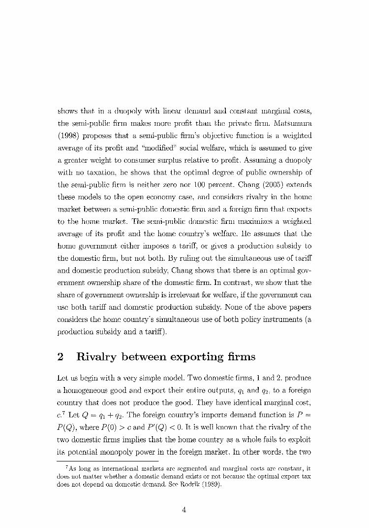
shows that in a duopoly with linear demand and constant marginal costs,

the semi-public firm makes more profit than the private firm. Matsumura

(1998) proposes that a semi-public firm's objective function is a weighted

average of its profit and "modified" social welfare, which is assumed to give

a greater weight to consumer surplus relative to profit. Assuming a duopoly

with no taxation, he shows that the optimal degree of public ownership of

the semi-public firm is neither zero nor 100 percent. Chang (2005) extends

these models to the open economy case, and considers rivalry in the home

market between a semi-public domestic firm and a foreign firm that exports

to the home market. The semi-public domestic firm maximizes a weighted

average of its profit and the home country's welfare. He assumes that the

home government either imposes a tariff, or gives a production subsidy to

the domestic firm, but not both. By ruling out the simultaneous use of tariff

and domestic production subsidy, Chang shows that there is an optimal gov-

ernment ownership share of the domestic firm. In contrast, we show that the

share of government ownership is irrelevant for welfare, if the government can

use both tariff and domestic production subsidy. None of the above papers

considers the home country's simultaneous use of both policy instruments (a

production subsidy and a tariff).

2 Rivalry between exporting firms

Let us begin with a very simple model. Two domestic firms, 1 and 2, produce

a homogeneous good and export their entire outputs, q1 and q2 , to a foreign

country that does not produce the good. They have identical marginal cost,

c. 7 Let Q q1 q2 . The foreign country's imports demand function is P =

P(Q), where P(0) > c and P'(Q ) < 0. It is well known that the rivalry of the

two domestic firms implies that the home country as a whole fails to exploit

its potential monopoly power in the foreign market. In other words, the two

`As long as international markets are segmented and marginal costs are constant, itdoes not matter whether a domestic demand exists or not because the optimal export taxdoes not depend on domestic demand. See Rodrik (1989).

4

firms over-produce. When both firms maximize profits non-cooperatively, the

socially optimal policy is to impose an export tax, at the same rate for both

firms.

Consider now the case where one firm is semi-public and has the objective

function of maximizing a weighted average of its own profit and the home

country's welfare, with weights 1 — 0 and 0, respectively. In this context,

we ask the following questions: should the export tax rates be different for

the two firms, and should they depend on B? Our answer for each of these

questions is "no." We now proceed to prove this "invariance theorem."

Let us note that if the home country can directly control the outputs of

the domestic firms, it will choose Q to maximize social welfare, which is the

export revenue minus the production cost:

W = P(Q)Q-cQ .

The socially optimal industry output, denoted by Q*, must therefore equate

the marginal export revenue with the marginal production cost:

P(Q*)Q* + P(Q* ) = c. (2)

As usual, we assume that the second order condition is satisfied. Let us start

with the standard case of two domestic firms which are privately owned.

Suppose that direct control is not possible. The home government can choose

an export tax t to influence the quantity exported. Assume the firms behave

as Cournot rivals, and that each wants to maximize its profit. Firm i's profit

function (net of tax) is

P(qi + q-i)qi — cqi — tqi. (3)

For this simple case, we obtain

Lemma 1 The socially optimal tax is equal to

—(Q*/2)P'(Q*) > 0. (4)

5

Proof: See Appendix A.1.1.8

Consider now the case where firm 1 is partly state-owned. We assume its

objective is to maximize a weighted average of its profit as given by (3),

and social welfare W, as given by (1). Let 0 E (0, 1) be the weight attached

to social welfare. Since the good is not consumed in the home country, so-

cial welfare is just the export revenue minus production cost. Thus firm l's

problem is:

max(1 — 0) [P(qi + q2)q1 — cq 1 — tq1 ] + 0 [P(q1 + q2)(q1 + q2) — c(q1 + q2)]

We assume that firm 1 takes t and q2 as given and may derive the following

invariance result:

Proposition 1 The social optimum can be achieved as a Nash equilibrium

by applying an optimal export tax. The optimal export tax is independent of

the parameter 0 that represents the degree of public ownership. At the optimal

tax, the Nash equilibrium output of each firm is independent of 0.

Proof: see Appendix A.1.2.

Remark 1 Proposition 1 can be generalized to the case of n domestic firms

that are Cournot rivals, of which m < n firms are semi-public.

Proposition 1 is a surprising and important result. Its intuition can be

best explained by considering the case of a completely state-owned firm. This

firm would maximize welfare, and any tax, including the optimal export tax,

would not influence its behavior because government tax revenues and the

firm's tax bills cancel out for welfare. Hence, given that the privately owned

firm produces half of the socially optimal output, a completely state-owned

firms would also produce half of the socially optimal output. Proposition 1

demonstrates that the optimal tax guarantees also that any partially state-

owned firm will keep this level as it has no incentive to produce less or more.

Obviously, these results extend easily to the case of more than two firms.

Lemma 1 coincides with Rodrik's (1989) optimal export tax for the case of only twofirms.

6

3 Rivalry in home market

We now turn to the case where the rivalry takes place in the home mar-

ket which is assumed to be segregated from the foreign market. We assume

constant marginal costs, so that output decisions for the home market are

unrelated to output decisions for the foreign market. This allows us to focus

on the home market. The home market is served by a domestic firm, firm 1,

and a foreign firm, firm 2, located in country 2. The quantities they supply

to the home market are denoted by y (domestic production) and x (export

by firm 2), respectively.

There is a literature that deals with optimal tariffs to extract rent from a

foreign monopolist (e.g. Katrak, 1977, Brander and Spencer, 1981 and 1984).

These authors assume that there are no domestic firms that can produce or

compete with the foreign monopolist. Assuming the home country's choice

variable is a tariff rate t, Brander and Spencer (1984) show that the optimal

tariff is positive if the domestic demand curve is not too convex and the

foreign firm's marginal cost is constant or increasing. On the other hand, if an

increase in tariff causes a larger increase in the consumer's price (dp/dt > 1)

then an import subsidy is optimal.' The scenario where a domestic firm can

compete with the foreign firm is taken up by Pal and White (1998), but

they assume that the home government may use only one policy instrument:

either a production subsidy for the domestic firm, or an import tariff.'

In this section, we allow the home government to have recourse to both

production subsidy s and import tariff t, and study how the optimal pair (s, t)

changes with the degree of public ownership of the domestic firm. To facilitate

understanding of our results, it is useful to consider first the benchmark

case where the government can control the domestic output (by control and

command).

9 For example, under constant marginal cost, an import subsidy is optimal if —2 < I? <—1 where B Qp" 1p'.

Schjelderup and Stahler (2005) consider the role of commodity taxes in atrade model under different rules of taxation.

7

Let Q = x y where y is produced by a domestic firm and x is the

quantity exported by the foreign firm to the home country. To make the

problem non-trivial, we assume the marginal cost of the home firm is higher

than that of the foreign firm, i.e., c1 > c2 . Otherwise the optimal quantity

imported would be zero. Let A c 1 — c2 denote the cost disadvantage of

the domestic firm. The domestic inverse demand function is p = p(Q), where

p(0) > c1 and p' (Q) < 0. As usual, we assume

p'(Q) + xp"(Q) < 0

for all Q > 0 and all x E [0, Q. Suppose the home government can precommit

the domestic output y and the tariff rate t. Appendix A.2.1 proves

Lemma 2 Domestic welfare is equal to

.x+y

W = f p(Q)dQ c1y [c2x x2p'(x+ y)]EF

Expression F is the cost (to the home country) of obtaining x. Since the

foreign production cost is c2x, we can interpret —x2p'(x+ y) p as the

the rent accrued to the foreign firm. For a given x, if domestic output y

increases, the rent accrued to the foreign firm will change by py = —x2p" .

Hence, an increase in domestic production will increase (decrease) the foreign

firm's rent if the inverse demand curve is concave (convex). Armed with these

prerequisites, we are now able to explain our next proposition.

Proposition 2 1. It is optimal to import if and only if the domestic firm

has a cost disadvantage, i.e., A > 0.

2. Assume an interior solution. (i.e. x* > 0 and y* > 0). At the optimal

consumption level Q*, given that A > 0, consumer price exceeds (re-

spectively, falls short of) marginal cost of the domestic firm if and only

if p"(Q*) < 0 (respectively, p"(Q*) > 0.)

Proof: see Appendix A.2.1.

8

The intuition for part 1 of Proposition 2 is straightforward. As for part 2,

the government has to balance two conflicting incentives, i.e., to increase do-

mestic consumption and to extract rents from the foreign firm. If the demand

function is linear, both effects cancel each other such that the consumer price

must be equal to the marginal cost of the domestic firm . This equality does

not hold if p(Q) is strictly concave or convex. If the inverse demand curve

is strictly concave (p" < 0), an increase in domestic production will increase

the rent accrued to the foreign firm at any given level of x. In such a case,

the home country refrains from expanding domestic output toward the level

that would equate price to marginal cost. It lowers domestic output so as

to extract more rent from the foreign firm. On the contrary, if the inverse

demand function is strictly convex (p" > 0), more domestic output will ex-

tract more rent from the foreign firm. Our next lemma gives the tariff which

manages trade optimally.

Lemma 3 Assume the government can directly control the output of the do-

mestic firm. The optimal tariff is

t* = 1 1 + (6)A Ap"

2(0 22 (2*

where R is the elasticity of the slope of the inverse demand curve;

crpl,R .

Proof: see Appendix A.2.1.

Note that R > 0 if p(Q) is a concave function. It follows from Lemma 3

that the optimal tariff is positive if and only if Do < (x*/Q*)R < —1, i.e.,

if the demand curve is not too convex.' This is a less demanding condition

than part 2 of Proposition 2. The reason is that a moderately positive tariff

may still result in a consumer price above the domestic marginal cost (recall

that c1 > c2).

11It follows that when there is no domestic production, the condition for a positiveoptimal tariff is oo > R > —1, which is consistent with Brander and Spencer (1984, p.231.)

9

The optimal output levels of both firms can be achieved by decentralized

measures. First, consider the case where both the domestic firm and the

foreign firm maximize their profits and assume the optimal domestic output

y* is strictly positive. Instead of dictating y* to the domestic firm, the home

country can give the domestic firm a subsidy s* while maintaining the same

tariff t* as in (6):

Lemma 4 Assume the domestic firm's objective is profit-maximization. The

optimal subsidy is

Ay*p'2 + t* (7)

Proof: see Appendix A.2.2.

10

t* —2

is the sum of the domestic firm's profit, the domestic consumer surplus, and

the government revenue:

x+yW=¶(1)

p(Q)dQ- p(x+y)(x +y [tx-sy]. (9)

Upon simplification,

x+y

W = p (y + x) y — c1y + [f p(Q) dQ P(x Y) ( X + Y) tx. (10)

As firm 1 is partly state-owned, its objective function is

V( 1 ) = (1 — + 0w, (11)

and we arrive at

Proposition 3 Assume the domestic firm is semi-public, and 0 is the weight

it places on social welfare.

1. The optimal tariff is independent of the degree of public ownership and

equal to

This is positive if and only if oo < R < —1.

2. The optimal domestic production subsidy is equal to

s = —y*p' + 2(1A

— 0)

- ±ex.pt (q*)

Q* 1 —

3. The optimal subsidy is negatively related to the degree of public owner-

ship if and only if the optimal tariff is positive.

Proof: see Appendix A.2.3.

Proposition 3 shows that the tariff stays constant whereas the subsidy

goes down with public ownership if the tariff is positive. The reason is that

the government can commit to a tariff and a subsidy whereas a partially

state-owned firm cannot precommit to domestic production. Hence, only the

11

government is able to fully extract rents from the foreign firm. A partially

state-owned firm, however, competes against a foreign rival on a level play-

ing field and will only take into account the effects of its ouput on welfare

for the fixed tariff rate and the equilibrium import level. Hence, the change

in welfare as perceived by the semi-public firm will only include the change

in consumer surplus and the change in the foreign rent via price effects as

described by Lemma 2. It will ignore the decline in tariff revenues due to a

decline in imports because imports and domestic production are determined

simultaneously. Consequently, the marginal change in welfare due to increas-

ing domestic production will be larger (and positive) as perceived by the

semi-public firm compared to the government, leading to output expansion

beyond y* if the subsidy is not adjusted. Therefore, the government has to

reduce the subsidy with public ownership as it correctly anticipates that a

semi-public firm would produce too much under a subsidy designed for a

private firm.

4 Rivalry between a domestic and a foreignfirm in a third market

In this section, we re-examine the third market model under the complication

that the home firm is partly state-owned. There are two firms, denoted by

1 and 2, located respectively in the home country and the foreign country.

They export all their outputs to a third market. We start with the case in

which firms are Cournot rivals. For simplicity, assume the goods are perfect

substitutes. The inverse demand function is P = P(Q), where Q = q1 +

The subsidy-inclusive profit of firm i is denoted by (i) :

(z) P (41 q2)qi C(i) (qi ) Ir(i) (qi , qj) + siqi,

where si is the export subsidy rate set by country i. By assumption, the goods

are not consumed in the home country, and therefore there is no domestic

consumer surplus. The social welfare of country 1 is taken to be equal to the

subsidy-inclusive profit of firm 1 minus the cost of the subsidy:

12

W(1) = ar ( 1 ) — s1 g1 = r(1)(q1,q2).

As before, we assume that firm l's objective is to maximize a weighted aver-

age of Fr (1) and W (1) , i.e.,

V(1) (1 — 0)iF (1) + 0W(1) q2) + (1 —

Firm 2 (the foreign firm) seeks to maximize FF (2).

We consider a two-stage game. In the first stage, the government of coun-

try 1 sets the export subsidy rate s1. (We assume s2 is exogenous, which we

set at zero for simplicity.) In stage 2, the firms simultaneously choose their

output levels to maximize their objective function. Furthermore, we assume

that the outputs are strategic substitutes, in the sense that an increase in

the output of one firm will reduce the marginal profit of the other firm:12

Assumption 1 Outputs are strategic substitutes:

02-Fr (i)(i) qiP"(Q) + -11Q) <dqidqi

for all qi E [0, Q] and for all Q > 0.

Given Assumption 1, we can now derive

Proposition 4 In the case of international Cournot rivalry in a third mar-

ket, the optimal rate of export subsidy is an increasing function of the degree

of state ownership 0. The outcomes (in terms of export quantity and social

welfare level) are however independent of the degree of state ownership.

Proof: see Appendix A.3.1.

We can demonstrate Proposition 4 by Figure 1. From the first-order con-

dition, we can derive that dq1 I d0 < 0 holds for firm l's reaction curve (see

(A.30) in Appendix A.3.1), i.e., an increase in public ownership shifts firm l's

12 For the notion of strategic substitutes and complements, see Bulow, Geanakoplos andKlemperer (1985).

13

reaction curve to the left. In Figure 1, RR denotes the reaction curve without

public ownership and VV denotes the reaction curve with semi-public own-

ership." The optimal policy makes the domestic firm behave as if it were

a Stackelberg leader. SS denotes the optimal after-subsidy reaction curve

which is determined such that the output in equilibrium maximizes domestic

profits and hence the domestic iso-profit curve is tangential to the foreign

firm's reaction curve R* R* Since public ownership shifts the reaction curve

to the left, a higher subsidy is needed to put the semi-public firm in a posi-

tion such that it behaves in the Nash equilibrium as if it were a Stackerberg

leader.

This result seems to be surprising. Why does VV lie to the left of RR?

The semi-public firm acknowledges at least partially that the subsidy is not

part of welfare. At the same time, the semi-public firm competes against

its rival on a level playing field and cannot commit to a high output level.

Hence, public ownership weakens the influence of the subsidy as it cancels

out for the welfare component of firm l's objective function. Consequently,

the subsidy must be larger in order to achieve the same output levels as with

two private firms.

A similar analysis applies to the case of Bertrand rivalry (in the third

market) between a semi-public home firm and a profit-maximizing foreign

firm. As firms compete by prices, we now assume that the two goods are

imperfect substitutes. Let x(1) and x(2) denote the demands for outputs of

firm 1 and firm 2 respectively. The demand functions are assumed to be

x(1) = x(1) (p1 ,p2 ) and x (2) x(2)(p1,p2)

where pi is the price the consumers in the third market have to pay for one

unit of good i. We use the following notation:

= x(i) = dx(i) ( i ) 32 X (i) ( i ) a2 X(i) api 3 a X — pip , X — etc.

pj

and make

13 Reactions curves do not have to be linear or parallell to each other.

14

Assumption 2 Demand for good i decreases with p i . The goods are substi-tutes: an increase in pj will increase the demand for good i, where i j:

xi(i) < 0 and x(1) > 0.

The cost functions are denoted by C(i)(x(i)), and the government of coun-

try 1 levies an export tax t on x (1) . (As before, the foreign tax is exogenous

and set to zero for simplicity.) We denote by 11 (i) firm i's gross revenue minus

production cost:

I1 (i) P2) = Pi x(i) (Pi, P2) — C (i) [x(i) (Pi P2)]

We use the upper-case letter 11 ( ' ) to distinguish this function from the func-

tion ¶(i)(qi, q2 ) introduced in the Cournot rivalry case. Let 11 (i) denote the

after-tax profit function of firm 1:

fi( i)(pi, P2) = (Pi — t)x (1) (Pi, P2) — C (1) [x (1) (Pi P2)] -

Again, since there is no domestic consumer surplus, the social welfare of

country 1 is the sum of 11 (1) and the government's tax revenue:

W(1) (P1 P2) = fl(1) (Pi P2) + tx(i) (pi,P2) = IT(1)(Pi,P2)-

We assume that firm 1 is partly state-owned, and its objective is to maximize

V (1) , which is a weighted average of fl (1) and W(1):

V( 1) = (1 — 0)fi( 1 )(pi ,p2 ) + ow(1)(p1,P2) = II(1) (Pi, P2) — (1 — 0)tx(1)(pi,p2)

Firm 2, on the other hand, is privately owned, and seeks to maximize its

profit.

We consider a two-stage game. In stage 1, the government of country 1

sets t. In stage 2, given t, the firms simultaneously choose the consumer prices

p1 and p2 . Furthermore, we assume that prices are strategic complements in

the sense that an increase in the price of good j will raise the marginal

contribution of pi to the profit of firm i:

15

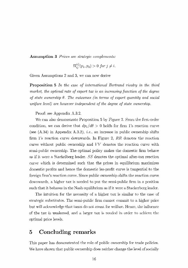
Assumption 3 Prices are strategic complements:

rii(3') (pi , p2 ) > 0 for

Given Assumptions 2 and 3, we can now derive

Proposition 5 in the case of international Bertrand rivalry in the third

market, the optimal rate of export tax is an increasing function of the degree

of state ownership 0_ The outcomes (in terms of export quantity and social

welfare level) are however independent of the degree of state ownership.

Proof: see Appendix A.3.2.

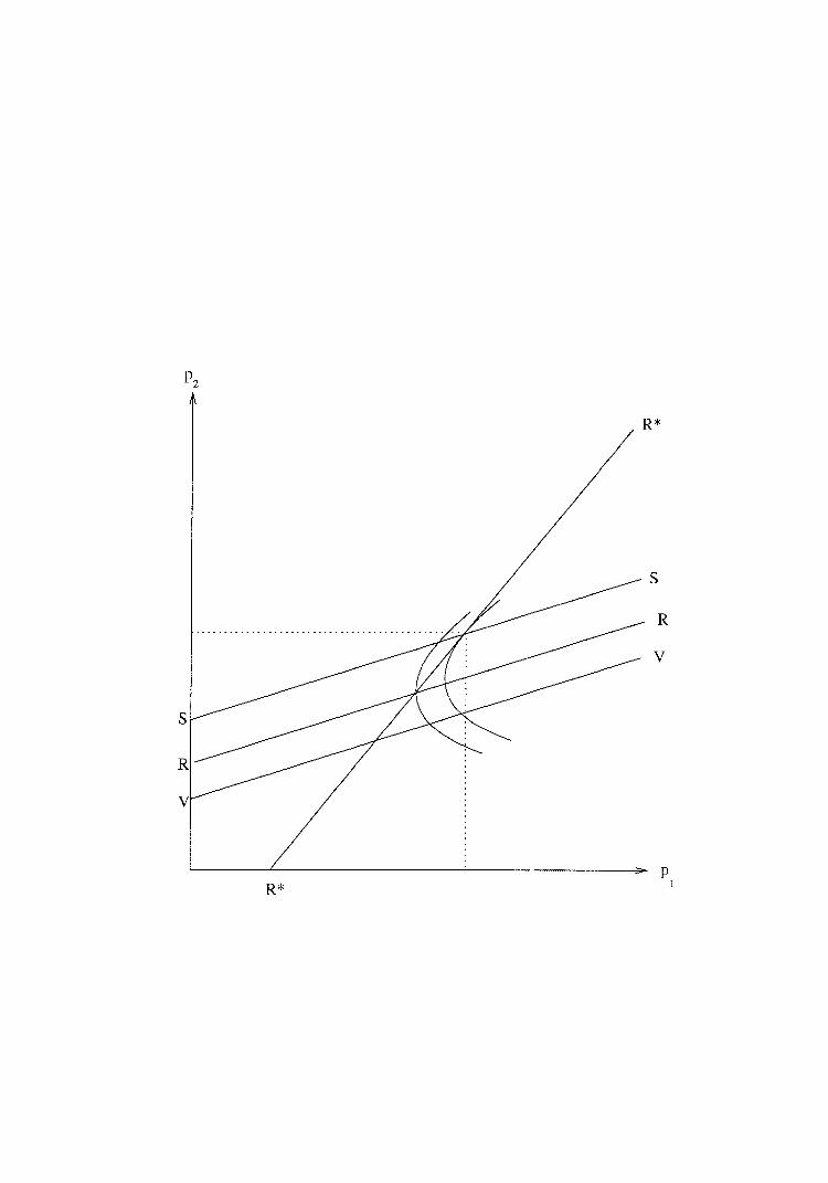
We can also demonstrate Proposition 5 by Figure 2. From the first-order

condition, we can derive that dp1 /d0>0 holds for firm l's reaction curve

(see (A.34) in Appendix A.3.2), i.e., an increase in public ownership shifts

firm l's reaction curve downwards. In Figure 2, RR denotes the reaction

curve without public ownership and VV denotes the reaction curve with

semi-public ownership. The optimal policy makes the domestic firm behave

as if it were a Stackelberg leader. SS denotes the optimal after-tax reaction

curve which is determined such that the prices in equilibrium maximizes

domestic profits and hence the domestic iso-profit curve is tangential to the

foreign firm's reaction curve. Since public ownership shifts the reaction curve

downwards, a higher tax is needed to put the semi-public firm in a position

such that it behaves in the Nash equilibrium as if it were a Stackerberg leader.

The intuition for the necessity of a higher tax is similar to the case of

strategic substitutes. The semi-public firm cannot commit to a higher price

but will acknowledge that taxes do not count for welfare. Hence, the influence

of the tax is weakened, and a larger tax is needed in order to achieve the

optimal price levels.

5 Concluding remarksThis paper has demonstrated the role of public ownership for trade policies.

We have shown that public ownership does neither change the level of socially

16

optimal activities nor the welfare level itself. It may, however, change thelevel of optimal trade taxes. If it does, we have shown that a semi-publicfirm cannot achieve the same results as the government on its own becauseit competes with rivals on a level playing field. This lack of commitmentdisqualifies public ownership as a tool for extracting rents from foreign firms.

Given our strong invariance results, the reasons why public ownershipis so prevalent seem to be obscure or at least beyond our model setup. Theassumption that the use of trade policy instruments is restricted does not helpin general. In particular, if subsidies for supporting your national championin a third market were restricted, public ownership would be harmful becauseit would make the domestic firm less aggressive. It seems that trade policycannot explain why firms are partially state-owned.

Acknowledgements: We have benefited from useful comments by JamesAmegashie, Hassan Benchekroun, Richard Cornes, Stephen Dobson, SteveDowrick, David Fielding, Michael Hoy, Alan King, Peter Kort, John Liv-ernois, Kim Long, Clyde Southey, and seminar participants at Tilburg Uni-versity, University of Otago, University of Guelph, and the Australian Na-tional University.

AppendixA.1 Rivalry between domestic exporting firmsA.1.1 The benchmark case: profit-maximizing duopolists

The first-order condition for firm i is

P'(qi + q_i )qi + P(q + q_i ) = c+t for i 1, 2. (A.1)

Assume that the second-order condition is satisfied, i.e., for all qi E [0, Q]and for all Q > 0, P"(Q)qi + 2P'(Q) < 0. The Cournot equilibrium outputsare denoted by qic(t). Let

2

Qc (t) =Y:qF (t).

17

Then, adding the two equations (A.1) for i = 1, 2, we get

.17)'(Qc (t))Qc (t) + 2P (Qc (t)) = 2(c + t)

To ensure that Qc (t) coincides with the socially optimal output Q*, the

government must set the export tax rate at t* according to (4). We now

verify that this tax rate makes each firm i produce the quantity qi = Q* /2.Firm i takes as given the tax rate t* and the output of the other firm, which

is q-i = Q*/2 (this turns out to be true in equilibrium). So its first-order

condition is

P (44 )q'4 P(qz = c+ t* c — (Q* /2)P'(Q*).

Clearly, by choosing qi = Q*/2, the firm satifies this condition. This argument

also applies to the other firm. It follows that, in a Cournot equilibrium with

the export tax rate t*, the equilibrium industry output is identical to the

socially optimal output.

A.1.2 The mixed-duopoly case

Suppose that the government sets the same t* as in the standard duopoly case

(see eq. (4)), and suppose that firm 2 chooses q 2 = Q*/ 2 as before (we will

verify that this is in fact the optimal choice for firm 2). Then the first-order

condition for firm 1 is

( 1 0) [P'(q1 +T) q1 P(q1— c — t*

0 {P1(q1 Q*+ -2 )( q1+ -) + P(qi + -4 - c} =0.2 2

Now, clearly, if firm 1 chooses q l = Q*/2, then the expression inside the

squared brackets is zero, because t* satisfies (4), and the expression inside

the curly brackets {...} is also zero, because Q* satisfies (2). Therefore the

first-order condition for firm 1 is satisfied at q1 Q*/2. The second-order

condition is

(1— 0) [qiP" 2P1+ 0 {QP" 2/3'} <

18

which is also satisfied. It remains to check that firm 2, by choosing q 2 =

Q*/2, also satisfies its own first- and second-order condition. This is easily

verified. q

A.2 Rivalry in the home marketA.2.1 The benchmark case: direct control of domestic output

The foreign firm takes y and t as given, and chooses the export quantity

x > 0 to maximize its profit:

max 72 = p(x y)x — (c2 t)xx> o

Assume an interior maximum for this problem. Then the first-order condition

isd7 2

xp,(x Y) P(x Y) — e2 — t = 0 .

dx

The second-order condition is

279' xp" < 0 (A.3)

which is satisfied because of (5). The second-order condition can be expressed

as

(A.2)

d272dx2

x

Q

- QpIn

p'> —2. (A.4)

From the first-order condition we obtain the foreign firm's reaction function:

x is expressed as a function of y and t. The function x = x(y, t) is implicitly

defined by

xpl (x Y) + P(x + Y) e2 t = 0.

The partial derivatives are

ax _ 1dt 2# xp" < °'

dx (p' xp") dx = Hp' + xP") < u.ay :7-- 2p' xP"

19

We can invert the function x = x(y,t) to get the function t = t(x, y). This

function tells us that, given y, if the home country wants the foreign firm to

supply x, the required tariff rate is

t(x, y) = xp'(x + + p (x + y) c2, (A.5)

Social welfare of the home country is the utility of consuming x + y minus

the cost of obtaining x + y, i.e..

W = p(Q)dQ — cry — _p(x + y) — x. (A.6)0

Substitute for t, using (A.5), we get

x-}-yW = p(Q)dQ el y — p(x + y)x + [xpi (x y) + p(x + y) — c2 1 x

which upon simplification leads to Lemma 2. q

The home country chooses x and y to maximize W . This yields two first

order conditions:

WW —OW

= p(x + y) — c1 + x 2p"(x y) < 0 ( = 0 if y > 0), (A.7)ay

ax147x — = p(x + y) — c2 x2p"(x + y) 2xp' < 0 ( = 0 if x > 0). (A.8)

W

Note that sufficiency is ensured if (i) x2p'(x y) is concave in (x, y), e.g.

if p' = —b < 0, and (ii) the integral is concave in (x,y), e.g. p(q) is linear.

Suppose we have an interior maximum (x* > 0 and y* > 0). Then the first-

order conditions become

Wy p(x + y) + x2p" (x y) = 0,

p(x + y) c2 x 2pll (x y) 2xp' = 0.

(A.9)

(A.10)

The second-order conditions are

Way = + x2pI" < 0, (A.11)

Wix = 2(p' 2xp") + (p' + x2p'") < 0 (A.12)

20

and

J WxxWyy (Wxy)2 = 2(0 2 + 2x2 [(pi )(pm ) 2(p")2 > 0. (A.13)

Condition (A.13) can be expressed as

Z x2pin 2'2 (7)1 2 < (A.14)

Example 1: Assume

p(Q) = e e c2 for Q E [0, 1]

Then p' = p" pM = — e Q , and J = 2e2Q (1 — x2 ) > 0 for

x < Q < 1.

We now prove part 1 of Proposition 2. First, we establish the why it is optimal

to import only if the domestic firm has a cost disadvantage. Subtracting

equation (A.9) from (A.10), we get

C i C2

x* (A.15)[-211(x* + y*)] [-2.71(x* + y*)]

It follows that x* > 0 only if A > 0 c1 > c2.

Next, we prove why it is optimal to import if the domestic firm has a

cost disadvantage. (If A > 0, then it is optimal to import a positive amount

from the foreign firm.) Suppose the contrary, i.e. A > 0 and yet x* = 0 and

y* > 0. Then equations (A.7) and (A.8) become, respectively,

AY') Cl = 0

P(Y*) c2 0

which implies c2 > a contradiction. As for part 2, substitute (A.15) into

(A.9):(ci — c2 ) 2 p"(x* + y*)

p(x* + y*) — +

= 0. (A.16)4 11(x* + y')j2

21

This equation determines the optimal total consumption, Q* L* + y*. We

assume that the equation

c1 — c2 ) 2 p"(Q*) = 0

4 :11(Q*)i2

has a unique solution Q* > 0 (e.g. the linear demand case, or see example 1

below). Eq. (A.17) gives Q* as a function of c1 and A, and it clearly shows

that p(Q*) > (<e1 if p"(Q*) < (>)0. q

Example 1 (continued): Assume c1 < e. Then equation (A.17)

yields Q* = In [4(e — c1 )/(4 A2 )] < 1. Using this, we obtain

E (0, Q*) and y* E (0, Q*) provided that e1 is sufficiently small

relative to A. In this case, p(Q*) > See the discussion of

Lemma 2 above for an explanation.

Given the optimal consumption Q* as determined by (A.17), we can compute

the derivative of Q* with respect to c1 and A. Re-write (A.17) as

ip'(Q*)1 2 p(Q) — + `2 p"(Q*) = D.

Differentiate totally to get

{[2( — c1)111)"1 P'1 3 TA2I) pn'} d P'12 del + p"dA = 0.

Using (A.16), (A.15) and (A.14), this equation becomes

(p') 2 ZdQ* (11) 2 dc1 +p" = 0,2

for which we getacr (A/2)p" < 0 if < 0 ,(A.18)aA 0302 Z

i.e., given c1 , a larger A will lead to greater consumption if the inverse

demand curve is concave; and

Q* I(A.19)

ac, = z

p(Q*) — ci + (A.17)

22

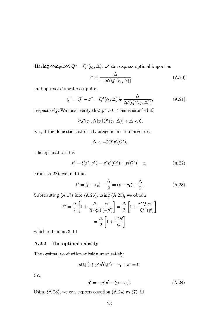
Having computed Q* = Q* A), we can express optimal import as

x* =A

and optimal domestic output as

y* = Q* — x* = Q*(cl A) + 211 (Q* (ci A))'

respectively_ We must verify that y* > 0. This is satisfied iff

2C2 * (ci A)P1 (Q * (ci . A)) + A < 0,

i.e., if the domestic cost disadvantage is not too large, i.e.,

A < —2Q*p r (Q*).

The optimal tariff is

t* = t(x* y*) = x* (Q*) + p(Q*) — c2.

From (A.22), we find that

t* = (p c2) A

= (p - A

.

Substituting (A.17) into (A.23), using (A.20), we obtain

—2p'(Q*(ci, A))(A.20)

(A.21)

(A.22)

(A.23)

A p" 1= A [ x* Pn1 +2 ( —p') ( —P') 2 Q (p')_

1 + R

which is Lemma 3. q

A.2.2 The optimal subsidy

The optimal production subsidy must satisfy

p(Q*) + y*P' (Q*) — c1+ s* = 0,

s* = — Y*11 — (p — c1). (A.24)

Using (A.23), we can express equation (A.24) as (7). q

*A2

1+

A2- Q

23

= t* = —L\ [12

'AP"2(p')2

(1 — 0) -s- 0Q*11(Q*) = s* +That is.

s* OVp' —y*p' A x*s =

1—B 1 — 0 2(1 — 0)or

Q*

(A.27)

0Q* pi—

A.2.3 Optimal subsidy and optimal tariff in a

Using (9) and (11), we get

x-hy

mixed duopoly

0 1) = 'T-r (1) 0 [f p(Q)dQ p(x + y)(x + y) + 0 [tx — sy]

e.,

01) = 7(1) +e-

p(Q)dQ — p(x + y)(x + y)1 + Otx + (1— 0)syjry

_ o

The first-order condition of firm 1 is

01,70-) = p + yp' — + (1 — 0)s — 0(y + x)p

dy

The first-order condition of firm 2 is

(A.25)

p + xi" — c2 — t = O. (A.26)

Clearly, the home country can achieve the same output pair (x*, y*) as in

the benchmark case, by setting the following tariff and subsidy vector

where t is identical to t* ands is a modification of s* (where s* is given by

equation (8)):

[ x* 1 * l q* )= — Y*11 + 2(1

A— 0) [Q* R

+ 0 x

1

p (

0— •(A.28)

It is easy to verify that given -s-", firm 1 will choose y*, if it expects firm 2

to choose x*. Similarly, given F, firm 2 will choose x*, if it expects firm 1 to

choose y*. It follows that the pair (x*, y*) is achievable as a Nash equilibrium,

by setting Ct '81 as in (A.27) and (A.28).

24

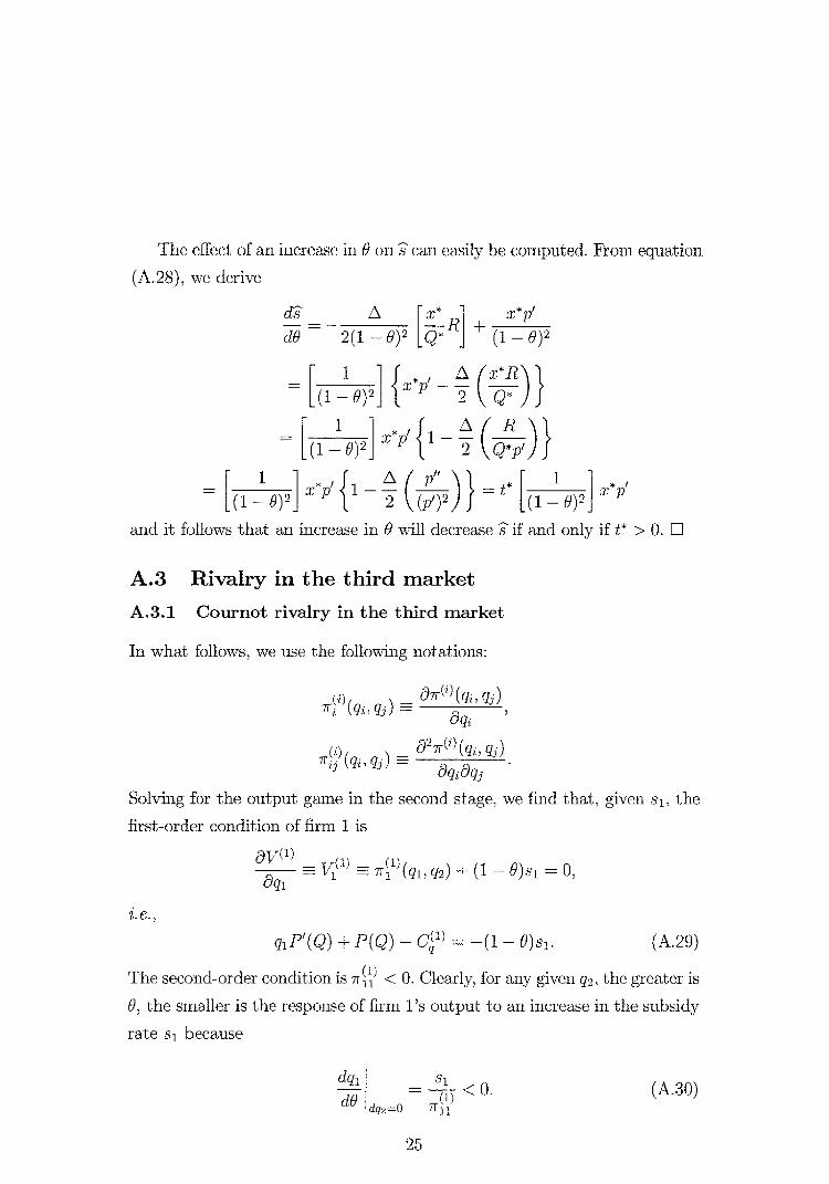
The effect of an increase in 9 on s can easily be computed. From equation(A.28), we derive

[ x* .T* pi

d0 2(1 — 0) [Q*' ± (1 — 0)2

[(1 19)2]

{ x„p' (x6; R*)}

[( 1 8) 2 1 x*Pi { 1 (Q1:11)}1

x*Pi { l Pll

*

(1 — 0) 2 , (/1 ) 2 )} t* [ l9) 2 -

x p9)22

and it follows that an increase in 0 will decreases if and only if t* > 0. q

A.3 Rivalry in the third marketA.3.1 Cournot rivalry in the third market

In what follows, we use the following notations:

0.7(i)(qi,qi)

( qi, qj) dqi027(i)(qi,

71"L ) (qi , q3 ) .dqidqj

Solving for the output game in the second stage, we find that, given s 1 , thefirst-order condition of firm 1 is

avo)agl

— V(1) 7(11)011 q2) + ( 1 — 0 ) 8 11=0,

e.

q1 .P 1 (Q) P(Q) — C,(1 1- ) —(1 — 0)s i . (A.29)

The second-order condition is 7r( 11) < 0. Clearly, for any given q 2 , the greater is9, the smaller is the response of firm l's output to an increase in the subsidyrate S i because

dqi sl0. (A.30)<

d0 (1)dq2=O ¶11

25

_(1) (1)7 11 71 12(2) (2)

712 722

- rig'dsi [ — (1 — 0)dq2 0ds1-

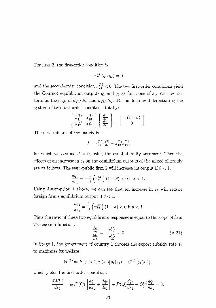
For firm 2, the first-order condition is

i2 (q1, = 0

and the second-order condition 71 22) < 0. The two first-order conditions yield

the Cournot equilibrium outputs q1 and q2 as functions of s i . We now de-

termine the sign of dq1 I ds i and dq2 I ds i . This is done by differentiating the

system of two first-order conditions totally:

The determinant of the matrix is

J= (1) (2) (2) (1)711 722 — 71'12 712

for which we assume J > 0, using the usual stability argument. Then the

effects of an increase in si on the equilibrium outputs of the mixed oligopoly

are as follows. The semi-public firm 1 will increase its output if B < 1:

dqi— (7r (2)

) (1 — 0) > 0 if 9 < 1.ds, 22

Using Assumption 1 above, we can see that an increase in s i will reduce

foreign firm's equilibrium output if 0 < 1:

dq21 ( 71

12)

(2)si

= —J

) (1 — 0) < 0 if 0 < 1d

Thus the ratio of these two equilibrium responses is equal to the slope of firm

2's reaction function:dq2 (2)dsi 11+12

dqi — (2) "

ds i 729(A.31)

In Stage 1, the government of country 1 chooses the export subsidy rate Si

to maximize its welfare

1/1/ (1) = P [qi(si), q2( 8 1)] '71( 8 1) — C(1) [ql (SO]

which yields the first-order condition:

d(1)dqi = (Q) + I 1+ P(Q) Ads idsi ds i uS1

dqiCql)dsi 7".=

26

Re-arrange terms to get

[qi Pt (C2) + P(Q) — CV ) ] = P' (Q)42ds ids,.

(A.32)

Using firm 1's first-order condition, eq. (A.29), we can re-write the social

optimal condition (A.32) as

—(1 — 0)si—dsi

= —q1.13'(Q)q2

.dsi

This equation gives the optimal rate of subsidy s i to the semi-public firm:

1(1 _ 0) qi P

' (C2)

dq2 dsidqi risi

1(1 _ 0) (Q)qii

(2)712

(2)722

(A.33)

where the second equality follows from (A.31). It follows that an increase

in 0 will increase .51 provided the value of the expression inside the curly

brackets remains constant when 0 changes. We now show that it in fact

does not change, if the optimal subsidy is imposed. To do this, it suffices to

show that the optimal subsidy always ensures that the stage-two equilibrium

output pair (qi , q2 ) is identical to the pair Nl", qn which would be obtained if

firm 1 were the quantity-setting leader, and firm 2 were the quantity-setting

follower." Re-write the optimal subsidy condition above as

(1 — 6)s7 = —q1PI(Q)„,,_(1)I ' 2

(2).7(2))

¶22

(71'12(2))

722

Using firm l's first-order condition, this gives

(2)( 1 ) (1) (¶12

¶2 (2)71-22

But this is precisely the condition that determines the pair (qf , which

would be obtained if firm 1 were the quantity-setting leader, and firm 2 is

the quantity-setting follower. q

14 It is well known that "the optimal export subsidy would move the industry equilibriumto what would be the Stackelberg leader-follower position with the domestic firm as theleader." (Brander and Spencer, 1985, Proposition 3).

27

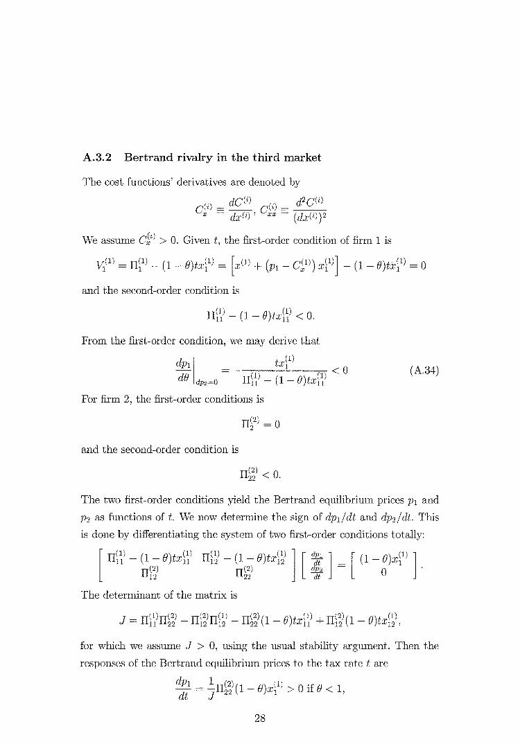
A.3.2 Bertrand rivalry in the third market

The cost functions' derivatives are denoted by

(j) dC(i) c(i) d2C(i)

dx( i ) (dx(i))2

We assume CV > 0. Given t, the first-order condition of firm 1 is

VP ) = it) — (1— 0)tx11) = [x (1) ± (P 1 – CV)) x11) - (1 — e)t±(,') = 0

and the second-order condition is

— (1 — o)tx(il,) < 0.

From the first-order condition, we may derive that

dp i t 1(1)X

d8 dp2 =0 fiVi) (1— 0)tx (1 11) < °

For firm 2, the first-order conditions is

1-1?) = 0

and the second-order condition is

n?2) < 0.

(A.34)

The two first-order conditions yield the Bertrand equilibrium prices pi and

P2 as functions of t. We now determine the sign of dpi I dt and dp 2 /dt. This

is done by differentiating the system of two first-order conditions totally:

[ it,',.) — (1 —9)txY`,) n(12) — (1— 8)tx12 - [dpi i (1— o)x(il ) 1 .

1-1(12)11

222) 42

{it a i

The determinant of the matrix is

j = 11(111)11v2) _ 11 .22) H(112) _ 11 V2) ( 1 _ 8)tx (i li) + n 12)

for which we assume J > 0, using the usual stability argument. Then the

responses of the Bertrand equilibrium prices to the tax rate t are

dpi (2

dt = –J H)

22 (1– 0)x(111 > 0 if 0 < 1,

(1 — 19)tx112) ,

28

[X

and hence

t* =(1 — 0)

1{ >0

dp2- -0)(1-o)x(11) > 0 if 0 < 1.

dt — j 12

The ratio of these two responses is equal to the slope of firm 2's reaction

function in the space (p 1 , p2):

dp2 H(2)dt = 12 > 0dpiT-T(2)dt 1122

In stage 1, the government of country 1 chooses t so as to maximize its welfare

w(1) (t ) = P1 (t ) X(1) (P1 (t), P2 (t))c(1) [X (P1 (t ), P2 (0)] •

The first-order condition is

dW(1) = x(1)

dpi (pi (t) — CV))

dt dt

Re-arranging terms yields

. 0.) dPi (1) dp2'21 ± x2 dt

= 0.

(1) +(p1— C(1) ) .T 1)1 .1)1d = (pi — C(1)) x(i)lP2dt 2 dt

(Pi — CP) x(1)02(1 — 0)tx‘ = 1 dpi

2 (it(1)

dt

and

hold. It follows that an increase in 0 will increase t* provided the term inside

the curly brackets does not change when 0 changes. We now show that this

term in fact does not change, if the optimal tax is imposed. To do this,

it suffices to show that the optimal tax always ensures that the stage-two

equilibrium prices (pi , p2 ) are identical to the prices (pi , /4), which would

be obtained if firm 1 were the price-setting leader, and firm 2 were the price-

setting follower. Re-write the optimal tax condition above as

(1 - 0)t' x(11) = (pi — C1(1) ) T9(1) II(122)If(222)(1}

(F422)

2H(2)"22

29

Using firm l's first-order condition, this gives

(2(1)2 "(2))

1122 )

12

But this precisely the condition that determines the prices (pf, pD, which are

obtained if firm 1 is the price-setting leader, and firm 2 is the price-setting

follower. q

References

[1] Chang, W.W., 2005, "Optimal Trade and Privatization Policies in an

International Duopoly with Cost Asymmetry", Journal of International

Trade and Economic Development, 14, 19-42.

[2] Brander, J.A. and B. Spencer, 1981,"Tariffs and the Extraction of For-

eign Monopoly Rents under Potential Entry,' Canadian Journal of Eco-

nomics, 14, 371-389.

[3] Brander, J.A. and B. Spencer, 1984, "Trade Warfare: Tariffs and Car-

tels," Journal of International Economics 16, 227-242.

[4] Brander, J.A. and B. Spencer, 1985, Export Subsidies and International

Market Share Rivalry, Journal of International Economics, 18, 83-101.

[5] Brander, J.A., 1995, "Strategic Trade Policy," in Handbook of Interna-

tional Economics, Volume 3. (eds: Gene Grossman and Kenneth Rogoff),

North Holland, Amsterdam.

[6] Bulow, J., J. Geanakoplos and P. Klemperer, 1985, "Multimarket oli-

gopoly: Strategic substitutes and complements ", Journal of Political

Economy, 93, 488-511.

[7 Conway, P., V. Janod and G. Nicoletti, 2005, "Product Market Regula-

tion in OECD Countries: 1998 to 2003," OECD Economics Department

Working papers, No. 419, OECD Publishing_

30

[8] DeFraja, G. and F. Delbono, 1989, "Alternative Strategies of a Public

Enterprise in Oligopoly," Oxford Economic Papers, 41, 302-11.

[9] Eaton, J. and G. M. Grossman, 1986, "Optimal Trade and Industrial

Policy under Oligopoly," Quarterly Journal of Economics, 101, 383-406.

[10] Fershtman, C., 1990, "The Interdependence Between Owership Status

and Market Structure: The Case of Privatization", Economica, 57, 319-

28.

[11] Fjell, K. and D. Pal, 1996, " Mixed Oligopoly in the Presence of Foreign

Private Firms," Canadian Journal of Economics, 29, 737-43.

[12] Haufler, A., G. Schjelderup and F. Stahler, 2005, " Barriers to trade

and imperfect competition: The choice of commodity tax base," Inter-

national Tax and Public Finance, 12, 281-300.

[13] Katrak, H., 1977, "Multinational Monopolies and Commercial Policy,"

Oxford Economic Papers, 29, 283-01.

[14] Matsumura, T., 1998, Partial Privatization in Mixed Duopoly, Journal

of Public Economics, 70, 473-83.

[15] Pal, D. and M.D. White, 1998, "Mixed Oligopoly, Privatization, and

Strategic Trade Policy," Southern Economic Journal, 65, 264-81.

[16] Pal, D. and M.D. White, 2003," Intra-industry Trade and Strategic

Trade Policy in the Presence of Public Firms," International Economic

Journal, 17, 29-41.

[17] Rodrik, D., 1989, "Optimal Trade Taxes for a Large Country with Non-

Atomistic Firms," Journal of International Economics, 26, 157-167.

[18] White, Mark D., 1996, "Mixed Oligopoly, Privatization, and Subsidiza-

tion," Economics Letters, 53, pp 189-195.

31

q2

P2

R* 1