Trade, Foreign Networks and Performance:

a firm-level analysis for India***

Alessandra Tucci

(Università degli Studi di Milano and Centro Studi “L.d’Agliano”)

This version August 28th 2005

Abstract

Using Indian firm-level data, this paper examines the combined role of import and export intensity in a context of foreign networks. From the relationship between international activities and simultaneity bias consistent productivity estimates we find that the more Indian firms are involved in trade networks the more they have a productivity advantage. Finally, information on the origin of import and on the destination of output are used to shed some light on the kind of networks in which firms are involved. We show that the upstream or downstream contact with more developed countries is not correlated with an higher productivity while there it seems to be an advantage for those firms that import and export to the same area.

*** I would like to thank Philip Keefer, Giuseppe Iarossi, Taye Mengistae and the WB Investment Climate Unit for hosting me as a visiting scholar and for providing the survey data which have been used under arrangements that respected confidentiality requirements. Furthermore I am grateful for helpful comments and suggestions to Giogio Barba Navaretti, Framcesco Daveri, Luca De Benedictis, to the participants to the CNR workshop in “Trade and Development economics” in Milano and to the Vth Doctoral Meeting in Internatiional Trade and Internatiional Finance organized by RIEF, CEPN and CEPII in Paris. Usual disclaimers apply. The author aknowledges the support of the Improving Human Potential Programme and the EC funded “Trade, Industrialization and Development” Research Training Network

1

Introduction

This paper analyses the performance of Indian firms that participate in international

networks defined by the combination of import and export shares. In addition,

systematic patterns of firm performance are identified after characterizing networks by

the specific origin of import and destination of export.

Here we are considering the firm’s upstream and downstream commercial linkages with

foreign countries as a whole. The activities shaping these foreign network are both

imports and exports as well as foreign ownership1 as already highlighted by Sjoholm and

Takii (2003).

Therefore, we use the combination of import and export intensities to assess the degree

of involvement of firms in trade networks. From this the relationship with firm

performance is explored controlling for foreign ownership. Specifically, using a

simultaneity bias consistent measure of performance levels2 we find that the more Indian

firms are involved in foreign networks the more they have a productivity advantage.

Export or import intensities of Indian firms have previously been studied by Hasan and

Raturi (2003) and by Driffield and Kambhampati (2003). The first two authors focus on

the determinants of export finding that greater usage of imported inputs influence export

volumes positively. While, for a sample of 1800 firms in the period 1987-1994, Driffield

and Kambhampati (2003), found that import intensity had a positive effect on efficiency

only for the textile industry while export intensity seemed to decrease efficiency in

sectors such as machine tools and chemicals.

Following the analysis on the degree of involvement of our firms in trade network, the

subsequent step of our work is the identification of the geographical characteristics of

these networks. Our data set has the nice feature of including detailed information on

the origin of imports and on the destination of exports. This information is useful to

investigate the characteristics of foreign networks, the nature of vertical specialization of

Indian firms and the relationship with performance.

1 This definition is different from the one used by Rauch (1999) that refers to “ties” and cultural proximity to define trading networks. 2 Derived applying the Levinshon and Petrin (2003) procedure.

2

Our main finding is that firms that are in contact with developed countries do not exhibit

a productivity advantage while firms that concentrate export and import activities

towards a specific area (both developed and developing) are more productive.

Regarding the performance of Indian firms with respect to trade, previous papers have

found mixed results. Topalova (2004), for the period 1989-2001, shows a positive

correlation between firm level productivity and the lowering of trade restrictions, in line

with Krishna and Mitra (1998) results. But besides Driffield and Kambhampati (2003),

also Parameswarn (2000), for a sample of 640 firms between 1989 and 1998, finds that

trade liberalization has had a negative effect on technical efficiency. For this, India

remains an interesting case study. Indian trade policy went trough a series of complex

reforms that started in the early 80s. Until 1982-83 Indian trade regime was

characterized by numerous quantitative restrictions. Then, in those years, the first step

towards liberalization lifted many restrictions on imports of intermediate inputs and

capital goods to promote technological upgrading and modernization of the Indian

industry. Then in the 1990s, following a balance of payment crisis, the continued reform

process showed a consistent commitment of the country towards trade liberalization. The

removal of quantitative restrictions on imports was accompanied by a gradual lowering

of customs duties in each of the budgets presented from 1991 onwards. However, even if

there is a wide recognition that the import-substitution industrial policy has been shifted

in favour of more liberalized import and export policies (Hasan et al 2003), the

protection level for Indian manufacturing at the end of the various phases of trade

liberalization still remains high (Das, 2003)3. On the other side, the country still

maintains a consistent domestic market therefore domestic firms are not necessarily

obliged to rely on foreign markets to exploit, for example, scale economies. Therefore

the combined analysis of import and export intensities can also have important trade

policy implications.

The rest of the paper is organized as follows Section 2 presents the theoretical

background on the relationship between import, export and performance. Section 3 then

contains the description of the dataset. In section 4 we present the simultaneity bias 3 From his quantification of Indian trade barriers Das (2003) finds for 2001 an average estimates for the “effective rate of protection” of 40 percent that it is very high if compared with the post reforms protection levels (average tariff rates of manufactures) of other developing countries: Indonesia (1999- 10.7%), Malaysia (1997- 7.5%) and Sri Lanka (1997- 19 %).

3

consistent production function estimates obtained with the Levinsohn and Petrin (2003)

methodology. Then, such firm level productivity measures are related to foreign

network indexes so to identify systematic component after controlling for observed and

unobserved plant characteristics and for industry heterogeneity. From this we report the

first results. Section 5 develops the analysis on the direction of trade. Finally, the last

two sections contain the causality and robustness checks and the conclusions.

2. Imports, exports and performance

In the most recent years, trade literature enriching the “new trade theory” models

à la Helpman-Krugman (1985) with firm heterogeneity has focused on the relationship

between international activities and firm performance. These previous representative-

firm models while taking into account imperfect competition, product differentiation and

increasing returns to scale, did not allow for the co-existence in the same sector of firms

that serve just the domestic market, firms that serve both the domestic and the foreign

markets and firms that are one hundred percent exporters. In fact, in such frameworks,

the exogenous industry characteristics induce all firms in the same sector to have the

same behaviour regardless their specific performances. The heterogeneous firm model,

on the contrary, relates the firm’s decision to its productivity level (e.g. Melitz 2003).

The development of this recent literature was inspired by many empirical studies on

micro data at the firm level4. In particular one consistent result of this empirical

literature is that, for all industrial sectors, exporting firms are more efficient than non-

exporting firms. This is combined with the proven existence of sunk entry costs into

foreign markets. Such costs, in addition to the per-unit trade costs, are mainly related to

information issues5. These stylised facts have been reconciled theoretically by Melitz

(2003), which shows how the fixed costs generate a self-selection of the most efficient

firms into foreign markets. This productivity dynamics is consistent with the findings of

Clerides, Lach and Tybout (1998) that have shown, for Colombia, Mexico and Morocco,

4 For example Roberts and Tybout (1997), Clerides, Lach and Tybout (1998), Bernard & Jensen (1999) and (2004), Kraay (1999), Aw, Chung and Roberts (2000), Van Biesenbroek, (2003) and De Loecker (2004). 5 A firm must find and inform foreign buyers about its products, learn about the foreign market and set up new distribution channels. Furthermore it must adapt its product to ensure that it conforms to foreign standards (Melitz 2003 and Roberts and Tybout 1997)

4

how the productivity trajectories of exporters were higher that those of non-exporters

already before starting exporting and they did not change thereafter. However on

empirical grounds the possibility that firms benefit from the contact with foreign

counterparts has not been ruled out. There are still studies presenting empirical evidence

of a learning-by-exporting effect on performance which materialize after breaking into

foreign markets (e.g. Kraay (1999), Van Biesenbroek (2003), De Loecker (2004),

Girma, Greenaway and Kneller, (2004) and Fernandes and Isgut (2005)).

Hence, the rich debate on the causal relationship between firm performance and

international trade is still open.

Such firm level literature mostly focused on exports (and foreign direct investment). In

this context, very few studies have considered the export counterpart, imports and

virtually no one has combined these two activities6. However, as pointed out by Ethier

(1982) and highlighted by Kraay, Soloaga and Tybout (2001), there are strict

complementarities between international activities of individual producers. Therefore

“studies that focus on one international activity at a time may generate misleading

conclusions” (Kraay et al, 2001, p.1).

Furthermore, not only exports have a linkage with firm’s performance but also imports

can be related to productivity. In fact, imported materials can be a source of learning7

and as Ethier (1982) noted, it can also be a way of expanding the menu of intermediate

inputs available to domestic firms favouring the best match between input mix and

desired technology or product characteristics. Hence at the firm level, we can consider

the generic “crossing the border” choice as driven both upstream and downstream by the

firm’s profit maximization process. In fact, the firm chooses the most efficient inputs’

source to minimize total costs in the production of an output that has to find its demand

domestically or abroad

Therefore our work contributes to the empirical analysis by examining, for a sample of

Indian manufacturing plants, the linkage between import participation and exporting

behaviour. Next, we relate the trade intensity index constructed combining import and

6 except for Bernard, Jensen and Schott (2005) that have highlighted the same gap in this the empirical literature. 7 There are few papers looking at the potential role of imports as a learning mechanism and at its impact on firm’s performance: Macgarvie (2003) for French firms, Keller and Yeaple (2003) for US multinationals and Blalock and Veloso (2004) for Indonesia.

5

export intensities8 to firm performance controlling for foreign ownership to find

evidence that firms involved in foreign networks both trough contacts with foreign

buyers and with foreign suppliers are advantaged with respect to other firms9.

These two variables have already been combined in the trade literature when studying,

on aggregated data, the relevance of the fragmentation of production processes across

borders (Yeats 2001) and of interconnectedness of production processes in vertical

trading chains across countries (Hummels, Ishii and Yi 2001). The first author finds that

the production-sharing component of all US manufacturing trade is 30 percent while for

Hummels, Ishii and Yi (2001) the growth in vertical specialization exports accounts for

25% or more of the growth in overall exports of OECD countries between 1970 and

1990, rising up to 50% for Mexico and Taiwan. These analyses are however limited to

the quantification of the phenomenon and the firm level implications of being involved

in such networks have not been explored jet.

3. Data and Descriptive Statistics

The data set used in this paper is based on a firm-level survey10 conducted by the

Development Research Group-Investment Climate Unit of the World Bank jointly with

the Confederation of Indian Industries (CII) and the Indian Council for Research on

International Foreign Relations. Two consecutive rounds of this Investment Climate

Survey have been conducted, in 2000 and 2002. The resulting balanced panel dataset

includes information on 188 firms belonging to five industries11, for five years (from

1997 to 2001)12.

8 Given that for firms there can be a coexistence of domestic and foreign activities, we focus on the share of output exported, rather than following the traditional approach of using, as main variable of interest, a dichotomous exporting status 9 It could be the case that firms more involved in foreign networks would be more productive because the combination of import and export engagements is associated with higher knowledge flows and more intense learning processes (MacGarvie, 2003) Or alternatively, the more productive firms, that self select into the export market, also choose to import some of their inputs in order to maintain their competitiveness. 10 For the sample design see Dollar, Iarossi and Mengistae (2002), Appendix A. 11 The industries covered are Garments, Textiles, Drugs and Pharmaceutical, Electronic Consumer Goods and Electric White Goods. 12 The small number of firms for which information is reported both in the first and in the second round of the survey is mainly due to high rates of “non response”. Therefore it is not possible to make any hypothesis on exit or on entry rates. For this reason, the analysis will be conducted on the balanced panel.

6

These surveys include plant-based13 data on sales and input purchases (together with

detailed information on export and import), labour and human resources, investment,

technology and R&D expenditures, ownership as well as data on objective aspects of the

investment climate.

Referring to the 188 firms for which there are five consecutive years of data, 71 percent

of them are exporter14, 38 percent of them are importers15 and combining the flows, 31

percent of the firms are both importers and exporters16. Considering the industry beak

down, we have 54 firms in the Drugs and Pharmaceutical sector17, 31 firms in the

Electronic Consumer Goods and the Electrical White Goods industries18 and 103 firms

in Textile and Garments sectors19.

Table 1 reports some descriptive statistics on the characteristics of the firms in the

sample. Consistently across sectors, exporters tend to be larger in size than the average

firm in the sample and importers are, on average, even larger than exporters. Regarding

the share of firms that have at least one foreign shareholder, this is higher among firms

engaged in trade practices and in particular, importers are more likely owned by foreign

individuals than exporters. The same pattern is followed by public ownership although

the share of firms that have a public shareholder is quite negligible in all the sub-

samples.

13 only one plant belonging to each firm is considered, even if the survey covers multi-plant firms 14 there are 133 firms for which, in the five years considered, the average ratio of total exports to total sales is positive. 15 There are 72 firms for which, in the five years considered, the average ratio of total imports to total inputs is positive. 16 There are 61 firms that for at least one of the years considered have both imported intermediate inputs and exported part of their output. 17 73 percent of them are exporters, 64 percent of them are importers and 53 percent are both importers-exporters. 18 45 percent of exporters, 21 percent of importers-only and 13 percent of both importers-exporters 19 76 percent of exporter, 19 percent are importers and 28 percent are both importers-exporters

7

Table 1. Descriptive Statistics on Selected Variables Average Number of employees

(Std Dev) Percent of Foreign owned firmsc) Percent of Public owned firmsd)

All sectors

Drugs &

Pharma

Electronic &

Electrical Goods

Garm. &

Tex.

All sectors

Drugs &

Pharma

Electronic &

Electrical Goods

Garm. &

Tex.

All sectors

Drugs &

Pharma.

Electronic &

Electrical Goods

Garm. &

Tex.

Total Sample

306,84 (856,81)

389,79 (646,97)

51,85 (80,17)

339,79 (1045,83) 11,7% 18,5% 3,2% 10,7% 2,1% 1,9% - 2,9%

Exportersa)

418,29 (996,72)

505,31 (720,96)

88,36 (102,72)

434,39 (1176,37) 16,5% 25% 7,1% 13,9% 3% 2,5% - 3,8%

Importersb) 615,41 (1283,74)

541,17 (751,59)

121,06 (124,44)

821,94 (1786,56) 22,2% 28,6% - 20,0% 4,2% 2,9% - 6,7%

a) Exporters are those firms that in the five years considered have on average a positive ratio of total exports to total sales. b) Importers are those firms that in the five years considered have on average a positive ratio of total imports to total

intermediate inputs. c) percentage of firms with a positive foreign ownership share. d) percentage of firms with a positive public ownership share.

As mentioned in the introduction, the main objective of this analysis is to explore in

details the role of import and export with respect to firm performance.

For this, we will concentrate on the degree of exposure to foreign markets. Specifically,

more than concentrating on binary variables to identify exporters and importers we will

use directly the share of output sold abroad and the share of intermediate inputs

imported. This way we want to diversify firms that are mainly oriented towards foreign

markets from those that beside being importers and/or exporters have also a relevant

share of domestic activities.

In Table 2 the descriptive statistics on import share and exports share show that the

average firm in the sample imports 10 percent of its intermediate inputs while it exports

almost 30 percent of its output. Considering that, in our sample, there are many firms

which buy intermediate inputs only from domestic suppliers, excluding the latter, the

average import share becomes much higher reaching 37 percent. The same thing

happens when the sample is restricted to exporters among which the average import

share is almost 70 percent higher than the overall mean.

Similar patterns are followed by the export share variable. However, confronting the two

sub-samples of importers and exporters it emerges that the average export share of

8

importers is quite close to their average import share while among exporters there is, on

average, a wider gap between the two measures in favour of export practices20.

In addition, 7 percent of the firms in our sample at least in one of the years considered

have imported all of their intermediate inputs and 28 percent have exported all of their

output. In the case of hundred-percent importers, the average export share is around 50

percent while the average import share of the hundred-percent exporters, is only 10

percent.

Table 2. Statistics on trade Variable Obs Mean Std. Dev Import Share 731 0,1044 0,2403 of Importers 203 0,3759 0,3258 of Exporters 389 0,1704 0,2911 Export Share 752 0,2792 0,3877 of Exporters 402 0,5222 0,3918 of Importers

203

0,3863

0,3829

Drugs and Pharmaceutical Import Share 209 0,1999 0,2953 Export Share 216 0,2345 0,3405

Electronic and Electrical Goods Import Share 121 0,0689 0,2102 Export Share 124 0,1129 0,2527

Textile and Garments Import Share 401 0,0653 0,2003 Export Share 412 0,3526 0,4235

A more rigorous analysis of these patterns is however called for. For this, we proceed

with the estimation of export decision equations following the literature on export

market participation (Bernard and Jensen (2004), Bernard and Wagner (2001) among

some) and we apply the same framework to the choice of importing, following

Macgarvie (2003).

20 This of course could reflect the fact that among importers, there is about 80 percent of exporters while among exporters there is only a 40 percent of importers.

9

Firms’ decision to export (import) depends on the fact that the current value of expected

profits from exporting (importing) exceeds the fixed cost incurred in changing the export

(import) status, Sit. This can be expressed with the following discrete-choice equation:

[ ]

>−=

otherwise 00E if 1 it

Yitit

SY π (1)

where Yit is the variable indicating export or import. Assuming that [ ] itYit S−πE is a

function of the factors affecting firm’s profitability and of an error term εit, the reduced

form binary choice equation becomes

>+++=

otherwise 00 if 1 Y

ititYit

Yit

XY ερδλ (2)

where Y is the variable identifying export or import status. δt is a time effect that should

capture the profitability conditions that are common across firms and ρi are time

invariant firm’s characteristics such as industry and location. According to the above

mentioned literature on the determinants of the firm’s export decision, the vector Xit of

firm’s characteristics includes employment, capital intensity, wages, the age of the firm

and technological proxies as age of machineries and the skill intensity. To avoid

causality problems all the firm’s characteristics variables are lagged one year. In

addition the share of foreign ownership controls for one of the possible channels that

would favour the export (or import) decision. With respect to the determinants of firm-

level imports there is much less research than on exporters’ characteristics, though

Kramarz (2003) finds that French importers are more capital-intensive and have lower

employment than non importers. Following Macgarvie (2003) that also studies French

firms we include in the import participation equation the same variables that we use to

model the export decision. In addition, to test for the fact that there is a linkage between

the activity of buying intermediate inputs from foreign suppliers and of selling output to

foreign customers, we also introduce the respective variables in the participation

equations.

10

Therefore after modelling the probability of exporting (importing) as:

)Pr()|1Pr( itYit

YYit

Y XXY ρδλε ++<== (3)

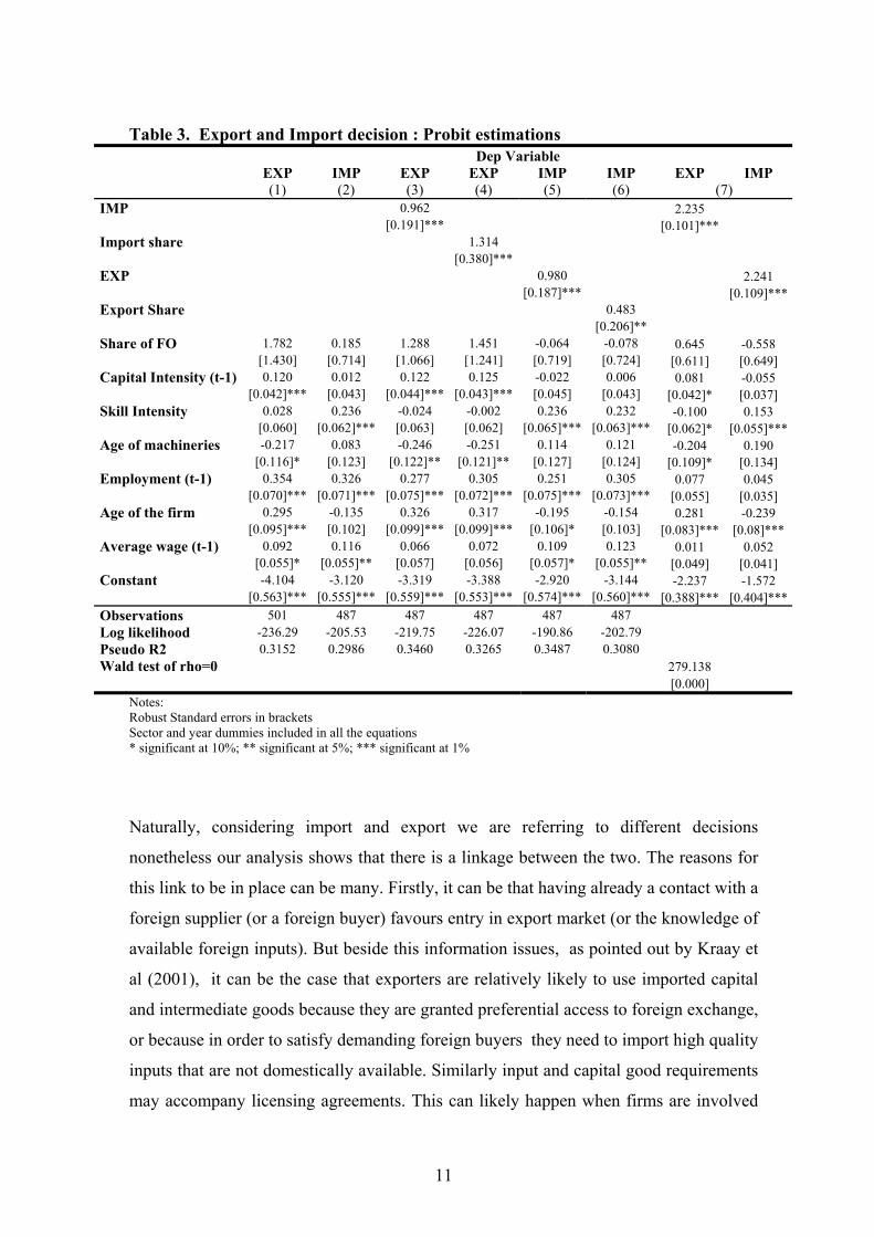
we estimate the firm’s propensity to trade with maximum likelihood. Table 3 displays

the results of the Probit model estimations of the baseline and of the augmented

specifications.

Interesting to note is that import and export are both positively correlated, respectively,

to the decision to export and to import. In the case of the export participation equation

import intensity has an even higher coefficient than the dichotomous variable (cfr.

column 4 and 5) which confirms the results of Hasan and Raturi (2003). The same

positive correlations are confirmed by the results reported in column 7 which

corresponds to the joint estimation of the two participation equation with a system

estimator21.

The coefficient on the foreign ownership variable is never statistically different from

zero while it seems that the capital and technology variables are positively correlated to

the export decision and negatively to the import decision. The first case is in line with

the findings of the literature while in the second case there it seems to be a substitution

effect between firm’s capital and technology and the capital and technology embodied in

the imported inputs.

21 Seemingly unrelated bivariate probit model.

11

Table 3. Export and Import decision : Probit estimations

Dep Variable EXP IMP EXP EXP IMP IMP EXP IMP

(1) (2) (3) (4) (5) (6) (7) IMP 0.962 2.235 [0.191]*** [0.101]*** Import share 1.314 [0.380]*** EXP 0.980 2.241 [0.187]*** [0.109]***Export Share 0.483 [0.206]** Share of FO 1.782 0.185 1.288 1.451 -0.064 -0.078 0.645 -0.558 [1.430] [0.714] [1.066] [1.241] [0.719] [0.724] [0.611] [0.649] Capital Intensity (t-1) 0.120 0.012 0.122 0.125 -0.022 0.006 0.081 -0.055 [0.042]*** [0.043] [0.044]*** [0.043]*** [0.045] [0.043] [0.042]* [0.037] Skill Intensity 0.028 0.236 -0.024 -0.002 0.236 0.232 -0.100 0.153 [0.060] [0.062]*** [0.063] [0.062] [0.065]*** [0.063]*** [0.062]* [0.055]***Age of machineries -0.217 0.083 -0.246 -0.251 0.114 0.121 -0.204 0.190 [0.116]* [0.123] [0.122]** [0.121]** [0.127] [0.124] [0.109]* [0.134] Employment (t-1) 0.354 0.326 0.277 0.305 0.251 0.305 0.077 0.045 [0.070]*** [0.071]*** [0.075]*** [0.072]*** [0.075]*** [0.073]*** [0.055] [0.035] Age of the firm 0.295 -0.135 0.326 0.317 -0.195 -0.154 0.281 -0.239 [0.095]*** [0.102] [0.099]*** [0.099]*** [0.106]* [0.103] [0.083]*** [0.08]*** Average wage (t-1) 0.092 0.116 0.066 0.072 0.109 0.123 0.011 0.052 [0.055]* [0.055]** [0.057] [0.056] [0.057]* [0.055]** [0.049] [0.041] Constant -4.104 -3.120 -3.319 -3.388 -2.920 -3.144 -2.237 -1.572 [0.563]*** [0.555]*** [0.559]*** [0.553]*** [0.574]*** [0.560]*** [0.388]*** [0.404]***Observations 501 487 487 487 487 487 Log likelihood -236.29 -205.53 -219.75 -226.07 -190.86 -202.79 Pseudo R2 0.3152 0.2986 0.3460 0.3265 0.3487 0.3080 Wald test of rho=0 279.138 [0.000]

Notes: Robust Standard errors in brackets Sector and year dummies included in all the equations * significant at 10%; ** significant at 5%; *** significant at 1%

Naturally, considering import and export we are referring to different decisions

nonetheless our analysis shows that there is a linkage between the two. The reasons for

this link to be in place can be many. Firstly, it can be that having already a contact with a

foreign supplier (or a foreign buyer) favours entry in export market (or the knowledge of

available foreign inputs). But beside this information issues, as pointed out by Kraay et

al (2001), it can be the case that exporters are relatively likely to use imported capital

and intermediate goods because they are granted preferential access to foreign exchange,

or because in order to satisfy demanding foreign buyers they need to import high quality

inputs that are not domestically available. Similarly input and capital good requirements

may accompany licensing agreements. This can likely happen when firms are involved

12

in international production networks importing intermediate goods that need to be first

reprocessed and then re-exported. Given the information available in the data set we

cannot detangle this issue, though we are interested in exploring the extent of

involvement of Indian firms in foreign networks22 and the relationship with their

performance.

4. Foreign networks

Once established that import and export decisions are correlated, we now focus

on the measurement of the involvement of Indian firms in foreign networks. For this we

construct and index that accounts for both import and export intensities.

The main reference is the “Vertical Specialization” index proposed by Hummels, Ishii

and Yi (2001) as measure of foreign valued added embodied in exports. This index is

constructed multiplying the export share by the value of imported intermediates.

Consequently, the firm level approximation of this index will be, for the firm i at time t:

tesIntermedia Imported Sales

ExportsExports*

SalestesIntermedia Imported

itit

itit

it

ititVS ⋅

=

= (4)

If the firm does not use imported inputs or it does not export, the index will be zero.

But for this version of the index23 there is not a definite upper bound and its value

can be highly influenced by the size of the firm: large firms that would import even a

small quota of inputs would exhibit an high value of the index. For this reason we

choose a firm level normalization of such index dividing by the material inputs used in

the production process. Thus, for the firm i at time t our index will be :

Sales

Exports*Inputs Material

tesIntermedia ImportedInputs Material

IE

==

it

it

it

it

it

itit

VS (5)

22 Identified both trough backward and forward foreign linkages. 23 In their paper Hummels, Ishii and Yi choose a sectoral normalization.

13

The main advantage of this second index is that it varies from zero to one. It is zero in

the case that the firm does not import any intermediate inputs or it does not export any

share of output. While, its upper bound is reached if all the inputs come from abroad

and, at the same time, all the output is sold in foreign markets. By some means, this

measure can be considered as a proxy for the extent of vertical integration of local firms

in foreign networks. In fact, this index will be higher the higher are both import and

export shares. For example if a firm imports 30 percent of its inputs and exports 70

percent of its output (or vice versa) the index will be 0,21 , lower than the case of a firm

with import and export intensities of 50 percent (0,25). This is because or index is meant

to combine the degrees of the upstream and the downstream linkages and the first case

corresponds to a firm mostly concentrated on the export linkage.

One other measure that is worth considering, because of its straightforward

interpretation, is the import content of export. Which, for the firm i at time t, will be

defined as:

Exports

tesIntermedia ImportedIE_sh

=

it

itit (6)

This measure is of great importance for trade policy. In fact, when designing trade

liberalization measures with the aim of boosting exports it is important to take into

account, how much domestic firms are dependent on imports. However, this measure

can be constructed only for exporting firms therefore excluding from the analysis

those firms that choose to serve the domestic market.

From Table 4, the average value of the IE index (5) appears to be not very high

showing how important is, in our sample, the weight of the firms that do not trade.

While the second index (6), calculated on the sub-sample of exporters appears

surprisingly high especially for the Drugs and Pharmaceutical sector highlighting the

high dependence on imported inputs.

Table 4. Degree of Vertical Integration

All sample Drugs & Pharmaceutical

Electronic & Electrical Goods Garment &Textile

Obs Mean Std. Dev. Obs Mean Std. Dev. Obs Mean Std. Dev. Obs Mean Std. Dev. IE 731 0,045 0,147 209 0,066 0,152 121 0,013 0,062 401 0,043 0,160

IE_sh 307 0,968 5,601 76 2,500 7,894 31 0.176 0.361 200 0,501 4,852

14

5. Empirical Methodology

From this, the next step will be to analyse the correlation between the trade practices of

the firms in the sample and their performances. In doing this we follow a standard two

step procedure. Firstly, we obtain productivity estimates. Subsequently, such measures

are regressed on the trade indexes constructed and on sets of firms’ characteristics.

Bernard and Jensen (1999) and Aw, Chung and Roberts (2000), among others, adopt this

two step approach in evaluating performance of exporters respectively for the United

States and for Taiwan and South Korea.

5.1 Productivity

Our measure of firm level performance is Total Factor Productivity calculated as

difference between the actual output and the one predicted by means of production

function estimations24.

Under the assumption of Hicks neutral Cobb Douglas technology we obtain the

following logarithmic approximation of the production function, for firm i , in industry j,

at time t:

j

itj

itj

itmj

itej

itkj

itbj

itwj

it meklblwy εωββββββ +++++++= 0 (7)

where yit is the log of gross output (proxied by sales)25 , kit is the log of the plant's

capital stock, lwit is the log of hours worked by skilled workers (white), lbit is the log of

hours worked by unskilled workers (blue), and mit and eit denote log-levels of materials,

and energy (which includes consumption of fuel and electricity). The error term has two

unobserved components, ωit ,the transmitted productivity components and εit,, the

random noise component. The difference between the two is that ωit is a state variable,

known by the firm when deciding the amount of input to employ in production26, while

24 Instead of TFP, an alternative measure of performance traditionally used is labour productivity. However as highlighted also by Sachs et al. (1999), given the country’s labour regulations, Indian firms often problems of over-staffing and this would bias the performance measure. 25 We did also estimated the value added production function, assuming weak separability on materials. The TFP estimations did not differ substantially. 26 But not by the econometrician.

15

εit is independent with respect to input choices. The correlation between the error

component and inputs leads to the well known simultaneity problem firstly highlighted

by Marschak and Andrews (1944). Estimators such as OLS that ignore this correlation

tend to overestimate the labour coefficient and underestimates the capital coefficient.

To overcome this problem we use the Levinshon and Petrin (2003) methodology27. This

approach builds on the work of Olley and Pakes (1996) that proposed the use of

investments as proxy to control for the correlation between the unobserved productivity

shock and capital (assuming that labour and materials are freely available inputs). The

Olley-Pakes procedure can be applied only to plants reporting non-zero investments and

this criteria would require a significant truncation of our sample28. For this reason, as

suggested by Levinshon and Petrin, we use intermediate input demand as proxy. In

particular, we use raw material inputs29 that become a valid proxy when their demand

function is monotonic in firm’s productivity for all levels of capital. Appendix A reports

the details of the Levinshon-Petrin estimation procedure, its implementation and a

description of the variables used in estimations.

The simultaneity bias consistent estimates of the production function’s parameters,

obtained for each macro sector, have then been used to calculate each firm’s Hicks-

neutral TFP as residual between actual and predicted output values. In order to make the

TFP estimates comparable across industries, the exponential values of TFP were divided

by the corresponding year and industry average30.

Table 5 reports descriptive statistics on the performance variables calculated dividing the

sample according to their trade practices. Both the TFP Index and the natural logarithm

of TFP show that exporters, importers and firms engaged in international networks are

on average more productive than firms that rely on the domestic market as source of

inputs and/or destination of output.

27 If the productivity is assumed to be plant specific and time invariant, the simultaneity problem can also be solved including in the regression firm specific effects (fixed-effect panel estimations). However this estimator does not fully exploit the cross-sectional variation which, especially in our case, with a short panel, is a relevant dimension. 28 In the case of the ICS of India, new investments are reported only for 1999 and 2001 and even in those case there is a high frequency of zero observations. 29 Alternatively also electricity consumption, possibly in physical quantities, can be a good proxy but we have only data on cost of energy. For a more detailed discussion on the choice of proxies see Appendix A. 30 To mitigate the problem of misreporting and outliers we used as industry-year TFP average the Huber mean truncating the one percent tails of the distributions.

16

Table 5 Relationship with performance Variable Obs Mean Std. Dev Obs Mean Std. Dev Importers Non Importers TFP_index 147 1,1736 0,5638 412 1,0384 0,5024 lnTFP 147 1,7392 1,4901 412 0,6662 1,3036 Exporters Non Exporters TFP_index 291 1,1389 0,583 284 1,0047 0,4289 lnTFP 291 1,1807 1,3891 284 0,7174 1,4438 IE>0 IE=0 TFP_index 119 1,2274 0,5795 440 1,0329 0,4982 lnTFP 119 1,7968 1,3708 440 0,7188 1,3641

5.2 Empirical Strategy and Results

The second step of our analysis consists in the estimation of the relationship between

trade practices and productivity. The baseline specification will be

ittiititit hkYXTFP νααααα +++++= 43210 (8)

Where the dependent variable represents the productivity index31 for firm i at time t; Xit

is our variable of interest that should be correlated with performance; Y is a set of time

variant firm’s characteristics such as the age of the firm, the ownership status, and size

but also other controls introduced in specific estimations that can explain firm

31 The production function that we have estimated using values to proxy for quantities could introduce a bias especially when firms operate in an imperfect competitive environment. In fact, the value of output does not depend only on technology but includes both prices and quantities. Since prices originate from the interaction of supply and demand, we have that sales includes the production side, the demand side and the market structure. For this reason, the above TFP estimates cannot be considered as pure measures of technical efficiency in production but more as measures of profitability. Keeping this in mind, we can still meaningfully employ in our analysis the TFP measures obtained by means of production function estimates using sales as proxy for output. In fact, the choices on import, export and diversification depend on expected profits. Profits will, in turn, depend both on productive efficiency and on the demand side characteristics such as product appeal, therefore using a measure of performance that captures profitability instead of productive efficiency will not bias the results.

17

performance; k are time invariant controls such as industry and location32, and h is the

set of year dummies that controls for macroeconomic shocks common to all firms. Our

main focus will be the magnitude and the sign of the α1 coefficient.

The first step is to analyse the relationship between productivity and Import and Export

intensity variables separately. The results from estimating equation (8) using standard

OLS correcting for heteroskedasticity are reported in tables 6 a and b.

The first and the second column of both tables show the regressions with the

dichotomous variables33. In particular, columns (1) are premium-type regressions were

the independent variables are all binary controls. The coefficients of the Import dummy

is never significant, while the coefficient on the export dummy is significant only if

other controls such as ownership status and firm age are not introduced. In contrast,

when import and export are introduced as “intensities”, columns (3), then both

coefficients become positive and significant indicating a positive relationship between

the productivity index and the share of inputs imported or the share of output exported

even though the results are not robust to the inclusion of additional controls such as

technology and innovation proxies.

In columns (4), the hypothesis of non linear (quadratic) relationship in import and export

share is tested and rejected.

Among the additional explanatory variables introduced, import experience (column 5 of

Table 6a) is the only one having a significant positive correlation with productivity.

This confirms the fact that it takes time to optimally integrate foreign inputs in the

production process. Export experience on the other side (column (5), table 6b) does not

have a similar impact.

As shown in column (7) in table 6a, there is a positive and significant correlation

between import intensity and productivity in the restricted sample of exporting firms. In

addition, column (7) in table 6b reports a positive and significant correlation between

export intensity and productivity in the sub-sample of importing firms.

32 To control for the location of firms, instead of dummies indicating Indian States, we use a dummy that assumes the value 1 if the firm is located in a coastal State, and a variable that quantifies, on a scale from 1 to 4 the investment climate of the State (World Bank and CCI, 2002) 33 Which take value one if the respective firm’s import share or export share are grater than zero, otherwise takes zero value.

18

Table 6a Relationship between Import and Performance Dependent variable : TFP_index

(7) (1) (2) (3) (4) (5) (6) exporters

0.086 0.070

Import Dummy [0.094] [0.085]

0.244 0.541 0.074 0.349 0.377 Import share [0.135]* [0.557] [0.204] [0.181]* [0.172]**

0.003 0.003 0.003 0.001 0.002 Age of the firm [0.005] [0.005] [0.005] [0.002] [0.002]

0.004 0.004 0.004 0.029 -0.001 Share of public ownership [0.002]* [0.003] [0.002]* [0.023] [0.001]

1.217 1.249 1.253 2.133 1.019 Share of foreign ownership [0.357]*** [0.377]*** [0.382]*** [0.441]*** [0.289]***

-0.346

Import share squared

[0.583]

0.002 Age of Machineries [0.004]

0.000 R&D_spending [0.000]**

0.013

Import experience

[0.003]***

0.002 Skill Intensity [0.005]

-0.371

Imported new investments

[0.255]

0.936 1.077 1.068 1.063 1.259 0.705 0.790 Constant [0.078]*** [0.083]*** [0.082]*** [0.080]*** [0.143]*** [0.103]*** [0.156]***

Observations 558 548 548 548 301 331 280

R-squared 0.05 0.09 0.10 0.10 0.25 0.20 0.08

Notes: Robust standard errors in brackets (clustered at the industry-year level) * significant at 10%; ** significant at 5%; *** significant at 1% , All the estimations include year sector, size and location controls .

19

Table 6b Relationship between Export and Performance Dependent variable : TFP_index

(7) (1) (2) (3) (4) (5) (6) importers

0.085 0.063

Export Dummy [0.039]** [0.047]

0.124 0.210 0.113 0.158 0.271 Export share

[0.070]* [0.385] [0.068] [0.102] [0.147]*

0.004 0.004 0.004 -0.001 0.001 Age of the firm [0.004] [0.004] [0.004] [0.002] [0.002]

0.005 0.005 0.005 0,031 0.002 Share of public ownership [0.002]* [0.002]** [0.002]** [0.024]** [0.002]

1.206 1.194 1.200 1.205 0.923 Share of foreign ownership [0.363]*** [0.393]*** [0.407]*** [0.406]*** [0.281]***

-0.090

Export share squared

[0.433]

0.003 Age of Machineries

[0.004]

0.000 R&D_spending

[0.000]**

0.004 Export experience

[0.005]

0.007 Skill Intensity

[0.004]*

-0.306 Imported new

investments [0.188]

0.940 1.101 1.102 1.105 1.285 1.068 1.133 Constant [0.076]*** [0.074]*** [0.079]*** [0.081]*** [0.088]*** [0.120]*** [0.612]*

Observations 573 563 563 563 359 334 146

R-squared 0.05 0.09 0.09 0.09 0.18 0.19 0.20

Notes: see Table 6a

The findings from this preliminary analysis substantiate further the importance of

investigating the combined role of import and export.

This is developed with the estimations reported in Table 7. Here, equation (8) is

estimated by substituting to X, first the dummy variable indicating the fact that a firm is

both an importer and an exporter, then the IE index as presented in the previous section.

As expected, both the interacted dummy and the IE index (5) display positive and

significant coefficient. This indicates that firms involved in foreign networks are more

productive and the higher is the degree of such involvement, the higher is productivity.

This results holds to the inclusion in the regressions of controls such as import and

20

export shares separately and also of variables indicating the export share of firms that do

not import their inputs and import share of firms that do not exports (column 5).

One other important and significant control is the share of foreign ownership that, as

expected, is positively correlated to the firm’s performance.

Yet, identifying the relationship between productivity and trade practices though the

variation across plants can introduce a bias. In fact the foreign network index could be

correlated with omitted plant characteristics that affect productivity. Under the

hypothesis that these characteristics are time invariant, it is possible to control for

unobserved firm heterogeneity with fixed effect estimates. This estimator identifies the

impact of the variable of interest relying on the within-firm time variation. Such

estimates are reported in column (6) and (7) where is shown how the coefficient on the

IE index remains positive and statistically significant.

To further test the robustness of our findings in column (8) we also introduce among the

regressors, the lagged value of TFP index assuming that firm’s productivity follows a

first-order Markov process. This inclusion introduces however a bias that we correct

trough the Arellano-Bond dynamic panel estimator34 in column (9). The coefficient of

interest maintains both significance and sign even when import and export shares are

introduced as controls (column (10)). This latter estimator has also the advantage of

permitting to address more general endogeneity issues. For this we introduce in the

GMM instruments matrix also the lagged values of the IE index to overcome the

endogeneity between the level of productivity and the value of the index. However the

use of lagged values of the variables to control for endogeneity leads to a significant

decline in the number of observations which does not permit to draw very definite

conclusions from the analysis. The same happens when using traditional instrumental

variables estimators such as the one reported in columns (11) and (12). The first case

corresponds to the two stages least squares estimator with first and second lag of the IE

index used as instruments. Column (12) instead displays the two-step instrumental

variables GMM estimates35 obtained with the same instruments. Nonetheless, in both

cases the IE index shows a positive and statistically significant coefficient and the tests

on the validity of the instrument confirm that they are uncorrelated with the error term36.

34 Arellano and Bond (1991) 35 The efficiency gains of this estimator relative to the traditional instrumental variable two step estimator derive from the use of the optimal weighting matrix that generates efficient estimates of the coefficients as well as consistent estimates of the standard errors in presence of heteroskedasticity. 36 therefore first and second lags are valid instruments for the IE index.

21

Table 7 Foreign networks and performance Dependent variable : TFP_index (1)a) (2) a) (3) a) (4) a) (5) a) (6) (7) (8) a) (9) (10) (11) (12) IMP*EXP DUMMY 0.129 0.204 [0.057]** [0.081]** Export Dummy 0.011 [0.056] Import Dummy -0.091 [0.114] IE 0.429 0.240 0.442 0.716 1.247 0.205 0.749 1.343 0.776 1.980 [0.108]*** [0.193]* [0.126]*** [0.284]** [0.353]*** [0.086]** [0.384]** [0.474]*** [0.324]** [1.201]* Import share 0.108 -0.553 -0.613 [0.174] [0.180]*** [0.240]** Export share 0.077 0.038 -0.006 [0.073] [0.082] [0.124] Imp. Sh. of non exporters -0.155

[0.119] Exp. Sh. of non importers 0.063 [0.084] TFP_index (t-1) 0.632 0.537 0.529 [0.123]*** [0.122]*** [0.120]*** Age of the firm 0.003 0.003 0.003 0.003 0.003 -0.001 0.001 0.001 -0.001 0.015 [0.002] [0.002] [0.002] [0.002] [0.002] [0.001] [0.001] [0.001] [0.002] [0.013] Share of public ownership 0.004 0.004 0.005 0.004 0.005 -0.020 0.000 0.000 0.002 0.450 [0.002] [0.002] [0.002]** [0.002]* [0.002]** [0.012] [0.000] [0.000] [0.005] [0.384] Share of foreign ownership 1.222 1.221 1.239 1.223 1.210 0.862 -0.042 0.040 1.158 3.483 [0.357]*** [0.355]*** [0.369]*** [0.391]*** [0.381]*** [0.269]*** [0.660] [0.652] [0.380]*** [2.073]* Constant 1.098 1.116 1.090 1.091 1.101 1.015 1.041 0.386 -0.078 -0.065 1.084 0.000 [0.066]*** [0.056]*** [0.064]*** [0.061]*** [0.063]*** [0.035]*** [0.041]*** [0.149]** [0.131] [0.129] [0.128]*** [0.000] Obs. 548 548 548 548 548 559 559 414 247 247 281 281 R-squared 0.09 0.10 0.10 0.10 0.10 0.02 0.05 0.51 0.14 Firm fixed effect Y Y Arellano Bond Y Y ARII P-value)

-0.07 (0.942)

-0.17 (0.861)

Hansen- Sargan test (P-value)

24.01 (0.021)

23.97 (0.019)

2.207 (0.137)

Hansen J (P-value)

1.380 (0.240)

Notes: Robust standard errors in brackets, a)Errors are clustered at the industry-year level. * significant at 10%; ** significant at 5%; *** significant at 1% All the estimations include year sector, size and location controls .

22

6 Does the direction of trade explain the positive effect of vertical

specialization?

These findings seem to substantiate the hypothesis that, at the firm level, there is a positive

relationship between performance and the involvement in foreign networks. Indeed not

only exports but also imports play a role with respect to performance. It can be the case

that in order to be successful in foreign markets as sellers, firms have to customize their

production and use imported inputs. In addition, importing intermediate inputs from

abroad firms can benefit from more advanced technology levels and from better quality

goods. Furthermore being contemporaneously an importer and an exporter a firm can

reduce the fixed costs linked to the gathering of information on foreign markets.

Our data do not allow to explain with more detail the kind of contractual relationship that

the firms in the sample have with their foreign counterparts. We only know the share of

foreign ownership of these firms and this is a factor that we have controlled for thorough

the whole analysis showing that there is a positive relationship with firm’s performance37

but it is not the main factor that explains it. However, a nice feature of the ICS survey is

that, for each firm, there are detailed information on the share of import sourced from

specific origin and the share of export to specific destination.

We will use this information to shed some light on the kind of international network in

which these firms are involved, or at least to have insights on the technological level to

which Indian firms are exposed, to better justify this productivity advantage of firm that

are both importers and exporters.

Next section will therefore presents some location-specific network indexes which have

been related to the performance indexes to identify systematic patterns.

6.1 Direction of trade

The information on the destinations and origin of goods traded refer to three main

geographic areas: “North” (which includes North America, Europe), “Asia” (which

includes also China and Japan), “South” (Central-Latin America, Africa, Eastern Europe,

37 In all the estimations the variable “Share of foreign ownership” shows a positive and significant sign.

23

Russia and Middle East) and finally, as a complement, also “Home” has been considered

so not to exclude from the sample the counterfactual.

From this, we construct localization-specific versions of the indexes presented in section

3.2, respectively on import and export practices separately and then on their combination.

For firm i at time t we have the share of intermediate inputs imported from each origin and

the share of export to each destination calculated as,

( )

=

=

it

itit

it

itit Inputs Mat.

X) from Interm. (Imported X from Imports of share*Inputs Mat.

Interm. Imported iX (9)

and

( )

=

=

itit SalesX) to(Exports X toExports of share*

SalesExports eX it

itit

it (10)

where X represents “North”, “South”; “Asia” and “Home”.

From this we then construct the localization-specific version of (5), for firm i at time t , is

defined as:

Sales

i toExports*Inputs Material

j from tesIntermedia ImportedEI ij

=

it

it

it

itit (11)

where j= “North”, “South”, “Asia” and “Home” and also i = “North”, “South”, “Asia”

and “Home”. Therefore, j indicates the origin of import, and i the destination of sales.

This index takes the value zero if the firm does not have contact with any of the two areas

considered. While it takes the value one, its upper bound, if a firm imports all of his

material inputs from the same area and sells all its output to the same area. Many firms in

our sample are not exclusively dealing with one single geographical area and this index

accounts for all the trade flows of each firms. If for example a firm buys 30 percent of its

24

inputs from the “North” and 70 percent from “Asia” and then it sells 40 percent of its

output domestically and 60 percent to the “North”, we have that the “Asia-North” flow has

the highest weight. In fact this firm is mostly characterized by having upstream contacts

with Asia and downstream contacts with the North. Even though the other flows38 are not

excluded from the analysis but they enter with a lower weight.

From the combinations of the four origin/destinations, sixteen kinds of flows are

generated. However for each flow there are too little non-zero observations to perform a

parametric analysis. For this reason we choose to group these flows according to different

criteria.

Firstly we concentrate on those flows that have the same origin and destination. This is to

test the idea that specialization towards a specific market generates the necessary

knowledge to overcome information and search costs. Therefore it permits to find the

most appropriate inputs and to better know the standards required to satisfy local demand

in order increase efficiency.

Thus, we construct an index that groups all the flows for which j=i excluding the domestic

cases39. Table 8a reports the results from the estimations obtained including these indexes

in equation (8). As expected, the index that measures the magnitude of import and export

flows to the same area shows a positive sign and it is statistically different from zero. The

sign and statistical significance is maintained also when controls such as import share,

export share or IE index are introduced.

In addition, column (4) displays the coefficient of the ratio between the index referring to

the same origin and destination and the IE index. This term gives a measure of the weight

of those international activities concentrated on the same areas with respect to all the

international activities. Such coefficient is positive and statistically significant indicating

that the correlation between performance and concentration persists regardless the amount

of international trade the firm is involved in as long as it is spatially concentrated.

However when we introduce lagged values of the variables as instruments, to solve the

possible endogeneity bias, the number of observations becomes fairly small and the results

become weaker (columns (6) to (10)).

38 “Asia-Home”, “North-Home” and “North-North”. 39 When j=Home and i=Home

25

Table 8a Direction of trade(j=i) Dependent variable : TFP_index

. (1)a) (2) a) (3) a) (4) a) (5)a) (6) (7) (8) (9) (10) IiEj (i=j) 1.041 0.921 1.013 0.815 0.449 0.470 0.781 3.219 3.017 [0.310]*** [0.339]** [0.363]** [0.426]* [0.576] [0.547] [0.612] [0.587]*** [0.502]***(IiEj)/IE (i=j) 0.274 0.121 -0.169 [0.066]*** [0.101] [0.109] Import share 0.046 0.100 -0.369 [0.108] [0.175] [0.184]** Export share 0.064 0.077 -0.014 [0.071] [0.074] [0.088] IE -0.157 0.039 -0.143 0.292 -0.170 [0.190] [0.107] [0.259] [0.346] [0.252] TFP_index (t-1) 0.770 0.667 0.722 [0.145]*** [0.142]*** [0.142]*** Age of the firm 0.003 0.003 0.003 0.003 0.003 0.001 0.001 0.001 0.001 0.001 [0.002]* [0.002]* [0.002]* [0.002] [0.002]* [0.001] [0.001] [0.001] [0.002] [0.002] Sh. of pub. Own. 0.005 0.005 0.005 0.004 0.005 0.000 0.000 0.000 [0.002]** [0.002]* [0.002]* [0.003] [0.002]* [0.000] [0.000] [0.000] Sh. of For. Own. 1.207 1.196 1.191 1.167 1.188 -0.001 -0.101 0.088 0.928 0.855 [0.356]*** [0.376]*** [0.378]*** [0.336]*** [0.345]*** [0.742] [0.711] [0.722] [0.362]** [0.479]* Constant 1.284 1.271 1.266 1.237 1.260 -0.021 -0.047 -0.052 1.079 0.000 [0.178]*** [0.181]*** [0.182]*** [0.165]*** [0.165]*** [0.092] [0.088] [0.093] [0.104]*** [0.000] Observations 548 548 548 548 548 255 255 255 283 283 R-squared 0.12 0.12 0.12 0.10 0.12 AB Y Y Y IV Y IV-GMM Y AR II (P-value) -0.84

(0.3995) -0.99

(0.3233) -0.57

(0.5699)

Hansen- Sargan test (P-value) 4.95

(0.4220) 5.69

(0.3371) 5.69

(0.3371) 0.206

(0.6496)

Hansen J (P-value) 0.3069

(0.5796)

Notes: Robust standard errors in brackets; a) Errors are clustered at the industry-year level. * significant at 10%; ** significant at 5%; *** significant at 1% , All the estimations include year sector, size and location controls.

Alternatively, the other issue of interest is tracing the flows that corresponds to contacts

with the “North”. This is to test the idea that those Indian firms that trade with developed

countries firms have contacts with the most advanced technology and having to face high

competition they should exhibit a better performance level. We group the location-

specific indexes according to the fact that “North” is at least one of the destinations or

origins of trade flows. Table 8b displays the results from estimations of the relationship

between this index and productivity. Surprisingly the coefficients on the variable of

interest are in most cases not statistically significant. Thus, we find no evidence that

generic trade contacts with North America or Western Europe are associated with a

productivity advantage.

26

Table 8b Direction of trade: highlighting “North” Dependent variable : TFP_index (1)a) (2) a) (3) a) (4) a) (5)a) (6) (7) (8) (9) (10) IiEj (i=N &/or j=N) 0.162 -0.110 0.076 0.066 -0.123 -0.111 -0.059 0.322 0.278 [0.043]*** [0.057]* [0.045] [0.045] [0.094] [0.090] [0.122] [0.099]*** [0.158]* IiEj /IE (i=N &/or j=N) 0.001 0.001 -0.001 [0.000]*** [0.000]*** [0.002] Import share 0.161 0.048 -0.365 [0.158] [0.162] [0.182]** Export share 0.082 0.058 -0.017 [0.071] [0.075] [0.088] IE 0.378 0.534 0.405 0.855 0.224 [0.228] [0.236]** [0.385] [0.468]* [0.440] TFP_index (t-1) 0.704 0.614 0.707 [0.149]*** [0.145]*** [0.149]*** Age of the firm 1.291 1.269 1.293 1.331 1.306 -0.007 -0.047 -0.007 1.113 0.000 [0.198]*** [0.195]*** [0.192]*** [0.199]*** [0.193]*** [0.100] [0.098] [0.100] [0.109]*** [0.000] Sh. of pub. Own. 0.003 0.003 0.003 0.003 0.003 0.001 0.001 0.001 0.000 0.000 [0.002] [0.002]* [0.002]* [0.002] [0.002]* [0.001] [0.001] [0.002] [0.002] [0.002] Sh. of For. Own. 0.004 0.003 0.004 0.005 0.004 0.000 0.000 0.000 [0.002] [0.002] [0.002] [0.002]* [0.002]* [0.000] [0.000] [0.000] Constant 1.167 1.168 1.177 1.200 1.196 0.109 0.006 0.198 0.907 0.857 [0.323]*** [0.356]*** [0.353]*** [0.352]*** [0.342]*** [0.719] [0.692] [0.723] [0.385]** [0.433]**Observations 540 540 540 540 540 251 251 251 279 279 R-squared 0.11 0.11 0.12 0.09 0.12 AB Y Y Y IV Y IV-GMM Y AR II (no autocorr.) (P-value) -0.40

(0.6876) -0.61

(0.5414) -0.33

(0.7398)

Hansen- Sargan test (P-value) 5.02

(0.4139) 4.68

(0.4557) 5.02

(0.4134) 3.875

(0.0491)

Hansen J (P-value) 1.259

(0.2618)

Notes: Robust standard errors in brackets; a) Errors are clustered at the industry-year level. * significant at 10%; ** significant at 5%; *** significant at 1% , All the estimations include year sector, size and location controls.

Summing up, the higher is the firms’ specialization, both as importer and as exporter,

towards a particular geographical area, the higher is their level of productivity. The

advantages do not seem to stem from the potential of technology transfer associated with

trade with developed countries or be generated by the efficiency requirements of these

markets, especially when considering downstream linkages.

7. Robustness checks: Semiparametric analysis

The parametric results reported up to here become weaker when we try to control for

endogeneity biases. The most interesting results derive from multivariate correlation

exercises. We are not able to conclude whether trade practices generate productivity

advantages or if it is the case that more productive firms chose to export and import.

However additional extensions of the analysis are suggested by the same heterogeneity of

27

firms within sector highlighted by the recent industrial organization literature. To

investigate this feature we examine whether the participation in trade networks affects the

distribution of firms’ productivity uniformly or not.

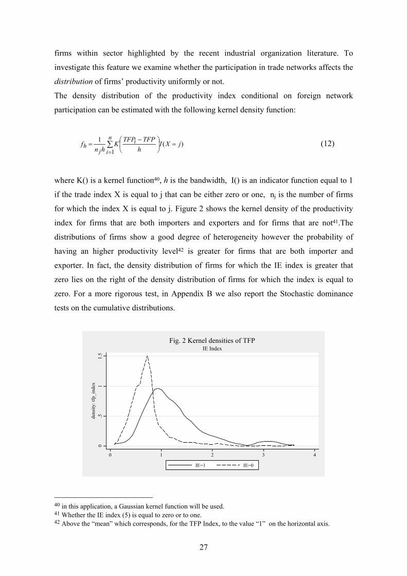
The density distribution of the productivity index conditional on foreign network

participation can be estimated with the following kernel density function:

∑=

=

−

=n

i

ij

h jXIh

TFPTFPKhn

f1

)(1 (12)

where K() is a kernel function40, h is the bandwidth, I() is an indicator function equal to 1

if the trade index X is equal to j that can be either zero or one, nj is the number of firms

for which the index X is equal to j. Figure 2 shows the kernel density of the productivity

index for firms that are both importers and exporters and for firms that are not41.The

distributions of firms show a good degree of heterogeneity however the probability of

having an higher productivity level42 is greater for firms that are both importer and

exporter. In fact, the density distribution of firms for which the IE index is greater that

zero lies on the right of the density distribution of firms for which the index is equal to

zero. For a more rigorous test, in Appendix B we also report the Stochastic dominance

tests on the cumulative distributions.

0.5

11.

5de

nsity

: tfp

_ind

ex

0 1 2 3 4

IE=1 IE=0

IE IndexFig. 2 Kernel densities of TFP

40 in this application, a Gaussian kernel function will be used. 41 Whether the IE index (5) is equal to zero or to one. 42 Above the “mean” which corresponds, for the TFP Index, to the value “1” on the horizontal axis.

28

On the other hand, these findings can derive from the different, and not observed,

characteristics of the firms that belong to the two groups. However, following Di Nardo et

al (1996) is possible to construct a counterfactual density distribution of the productivity

of firms for which the IE index is equal to zero. This counterfactual density is calculated

associating a greater weight to the firms that are not involved in international networks but

that have observable characteristics similar to those firms that are involved.

The density function of the TFP index conditional to the realization of the IE index is the

integral of the cumulative conditional probability function. For the case of firms that are

not involved in foreign networks but have the same zi characteristics of firms that are both

importers and exporters we have that:

( ) ( ) ( )∫∫ ===

======z

izz

iziz XzdFXzdFXzdFXzTFPfXzdFXzTFPfXTFPf )0|(

)0|()1|(0,|)1|( 0,|0| (13)

Thus, with )0|()1|(

==

XzdFXzdF =ψz(zi) as weighting function, the estimated counterfactual kernel

density function will be:

∑=

=

−

=n

i

iz

jh XI

hTFPTFPK

hnf

1)0(*ˆ1 ψ (14)

by applying Bayes rule at the numerator and at the denominator, the weighting function

can be estimated using the following specification:

)1Pr()0Pr(

)|0Pr()|1Pr(

)0|()1|()(

==

====

===

=XX

zzXzzX

XzdFXzdFz

ii

izψ (15)

Where, Pr(X=0) and Pr(X=1) are the unconditional probabilities that the IE index is

equal to zero or one respectively, while Pr(X=1| z = zi) and Pr(X=0| z = zi) are the

prediction obtained from Probit estimates of the probability that X=1 or X=0, with zi as

regressors43. Figure 3 displays the estimated counterfactual density for the firms that are

not involved in trade networks. This latter density lies between the other two showing how

the similarity on firm characteristics affects the distribution of the performance variable,

43 zi is a vector that includes the same variables used to estimate equation (3)

29

however it is still always on the left of the distribution of productivity of the plants that are

engaged in trade both upstream and downstream.

Therefore after controlling for firm characteristics we still find that there is an higher

productivity advantage associated with being both an importer and an exporter.

0

.51

1.5

dens

ity: t

fp_i

ndex

0 1 2 3 4

IE=1 IE=0IE=0 reweigh

IE Index and reweighted densityFig. 3 Kernel densities of TFP

Similar analyses have then be performed substituting to X, in equations (12) to (15), firstly

the index that identifies firms that have both upstream and downstream contacts with the

same geographical area, then the index that indicates trade flows with North America and

Western Europe. Results are displayed in Figure 4 and 5.

0.5

11.

5de

nsity

: tfp

_ind

ex

0 1 2 3 4

0.5

11.

5de

nsity

: tfp

_ind

ex

0 1 2 3 4tfp_index

Same dest/originDifferent dest/originDifferent dest/origin - reweighted

Same Destination and reweighted densityFig. 4 Kernel densities of TFP

30

0.5

11.

5de

nsity

: tfp

_ind

ex

0 1 2 3 4 5

0.5

11.

5de

nsity

: tfp

_ind

ex

0 1 2 3 4 5

North=1North=0North=1 reweighted

Trade with North and reweighted densityFig. 5 Kernel densities of TFP

These last two figures (and the stochastic dominance tests reported in Appendix B)

confirm the findings of the parametric analysis on the direction of trade. In fact, after

controlling for firm characteristics, the density distribution of productivity associated to

trade flows that have the same origin and destination always lies on the right of the density

distribution of productivity associated to other flows (Fig.4). While in the case of trade

flows with the “North” there seem to be no diversification between the density

distributions (Fig.5).

Conclusions

Indian exporters and importers have higher productivity than firms that are not engaged in

these practices. This replicates similar findings for a number of other countries.

Specifically, we find that such positive correlation with performance is stronger and more

significant when the share of inputs imported or the share of output exported are

introduced substantiating the idea that markets are segmented and it is necessary to

specialize both as a “buyer” and as a “seller”. Therefore the more a firm is oriented

towards foreign markets, the more advantages it can reap given also the fact that there are

fixed costs in entering foreign market that need to be compensated. Moreover the most

productive firms are those that choose to have both backward and forward linkages with

31

foreign counterparts. In particular, the higher is the magnitude of the combined flows that

involve the same region the higher is the efficiency advantage. This combined effect of

imports and exports within trade networks on firm performance has not being documented

before and it deserves further investigation.

Besides, further analysis on the relationship between import and exports can have

important trade policy implications. India has moved from an import-substitution

industrial policy to more liberalized import and export policies. However the country

liberalization process is not yet completed and for this it can be relevant to focus on the

import content of export at the firm level.

Finally from the analysis on the origin and destination of trade it has emerged that firms

that are exporter-to or importer-from North America and Western Europe do not

necessarily have a productivity advantage with respect to the others. This is quite

surprising if we interpret the results on the light of previous studies. However this could

correspond to the involvement of Indian firms in production networks with Northern

firms. Given the possibility of extreme disintegration of production processes we can have

that, theoretically, in a low-cost labour country like India, the more labour intensive and

lower value added phases of production are performed. This can be one of the reasons

why we do not find efficiency advantages. This issue needs however more in depth studies

in the future and more specific data sources.

32

References Antras, P. and E. Helpman (2004) “Global Sourcing”, Journal of Political Economy 112,

No. 3:552-80 Arellano, M and S. Bond (1991) “Some tests of specification for panel data: Monte Carlo

evidence and an application to employment equations” Review of Economic Studies, 58, 277-297

Arndt, S, and H. Kierzkowski eds. (2001) Fragmentation: new Production patterns in the World Economy, Oxford University Press

Aw, B. Y., S. Chung, and M. J. Roberts (2000) “Productivity and Turnover in the Export Market: Micro-level Evidence from the Republic of Korea and Taiwan (China)” World Bank Economic Review 14 (1), 65–90.

Bernard A.B., Eaton J., Jensen B. and S.S. Kortum (2000) “Plants and Productivity in International Trade”, NBER Working Paper No. 7688.

Bernard, A. B. and J. B. Jensen (1999) “Exceptional Exporter Performance: Cause, Effect, or Both?” Journal of International Economics 47 (1), 1–26.

Bernard A. and J. B. Jensen (2004), "Why Some Firms Export", The Review of Economics and Statistics, 86, No. 2: 561-69

Bernard A., Jensen J. B. and P. Schott (2005), "Importers, Exporters and Multinationals: a Portrait of Firms in the US that Trade Goods", NBER WP no. 11404

Bernard, A.B. and Wagner, J. (1997) “Exports and Success in German Manufacturing”, Weltwirtschaftliches Archiv 133, 134-57.

Blalock, G. and P. Gertler (2004) “Learning from exporting: Plant-level Evidence from Indonesia’s Trade Liberalization”, Journal of Development Economics, forhcoming

Blalock, G. and F. Veloso (2004) “Trade, Technology Transfer and Productivity Growth: the Neglected Role of Imports”, Discussion Paper, Cornell University mimeo

Clerides, S, S. Lach, and J. Tybout (1998) ”Is Learning by exporting Important? Micro-Dynamic evidence from Colombia, Mexico and Morocco”, Quarterly Journal of Economics, 113, 903-947

Confederation of Indian Industry and The World Bank (2002) “Competitiveness of Indian Manufacturing: Results from a Firm-Level Survey” by O. Goswami, A.K. Arun, S. Gantakolla, V. More, A. Mookherjee for CII and D. Dollar, T. Mengistae, M. Hallward-Driemier and G. Iarossi for the WB

Das D.K.(2003)“Quantifying Trade Barriers: has protection declined substantially in Indian manufacturing?” ICRIER WP No 105

De Loecker, J. (2004) “Do Exports Generate Higher Productivity ? Evidence from Slovenia” LICOS Discussion Papers No.151

Di Nardo, J., N. Fortin and T. Lemieux, (1996) “Labor market institutions and the distribution of wages, 1973– 1992:a semiparametric approach” Econometrica 64, pp.1001-1044.

Dollar, D. ,G. Iarossi and T. Mengistae (2002) “Investment Climate and Economic Performance: Some Firm Level Evidence from India” , Stanford University Center For Research On Economic Development and Policy Reform WP No. 143

Driffield, N. and Kambhampati, U. (2003) “Trade Liberalization and the Efficiency of Firms in Indian Manufacturing”, Review of Development Economics, 7, 419-430

Epifani, P. (2003) “Trade Liberalization, Firm Performance, and Labor Market Outcomes in the Developing World: What Can We Learn from Micro-Level Data?” World Bank WP No.3063

33

Ethier, W. (1982) “National and International Returns to Scale in the Modern Theory of International Trade”, American Economic Review ; 72, No. 3:389-405

Fernandes, A.M and A. E. Isgut (2005) “Learning-by-Doing, Learning-by-Exporting, and Productivity: Evidence from Colombia”, World Bank Working Paper no.3544

Girma, S., D. Greenaway and R. Kneller (2004)” Does Exporting Increase Productivity? A Microeconomic Analysis of Matched Firms” Review of International Economics (forthcoming)

Griliches, Z. and J. Mairesse (1998).”Production Functions: The Search for Identification” In S. Strom (Ed.), Econometrics and Economic Theory in the Twentieth Century: The Ragnar Frisch Centennial Symposium, pp. 169–203. Cambridge University Press.

Greenaway D., J. Gullstrand and R. Kneller (2003)” Exporting May Not Always Boost Firm Level Productivity” GEP Research Paper 2003/26

Hallward-Driemeier, M., Iarossi, G. and Sokoloff, K.L. (2002) “Exports and Manufacturing Productivity in East Asia: A Comparative Analysis with Firm-Level Data”. NBER Working Paper No. 8894

Hasan, R. (2002), “The Impact of Imported and Domestic Technologies on the Productivity of Firms: Panel Data Evidence from Indian Manufacturing Firms”, Journal of Development Economics, 69, 23-49.

Hasan, R. and Raturi, M (200), “Does Investing in Technology Affects Exports: Evidence on Indian Firms ”, Review of Development Economics, 7, 279-293.

Helpman, E. and P. Krugman (1985) Market Structure and Foreign Trade, Cambridge, and London, The MIT Press

Helpman E., Melitz J., and S. Yeaple (2004) “Export versus FDI” American Economic Review ; 94, No. 1:300-316

Hummels, D., J. Ishii, and K-M Yi, (2001), “The Nature and Growth of Vertical Specialization in World Trade,” Journal of International Economics, 54, 75-96.

Hasan, R., D. Mitra and K. Ramaswamy, (2003) “Trade Reforms, Labor Regulations and Labor-Demand Elasticities: Evidence from India,” NBER Working Paper 9879

Katayama, H., S. Lu and J.R. Tybout (2003): "Why Plant-Level Productivity Studies are Often Misleading, and an Alternative Approach to Inference," NBER WP 9617

Keller, W. and S. Yeaple (2003) “Multinational Enterprises, International Trade, and Productivity Growth: Firm Level Evidence from the United States,” Discussion paper, University of Texas, Austin, Dept. of Economics.

Klette, T.J. and Z. Griliches (1996): "The Inconsistency of Common Scale Estimators when Output Prices are Unobserved and Endogenous," Journal of Applied Econometrics, 11, 343-361

Kraay, A. (1999). Exportations et Performances Economiques: Etude d’un Panel d’Entreprises Chinoises. Revue d’Economie Du Developpement 0 (1-2), 183–207.

Kraay, A., Soloaga, I. and J. Tybout (2001) “Product quality, product efficiency and international technology diffusion” paper presented at the AEA meeting, New Orleans, January.

Kramarz, F. (2003) “Wages and International Trade” mimeo Krishna, P. and D. Mitra (1998) ‘Trade Liberalisation, Market Discipline and

Productivity Growth: New Evidence from India’, Journal of Development Economics, 56, 447-462

Levinsohn, J. and Petrin, A. (2003). “Estimating Production Functions Using Inputs to Control for Unobservables”, Review of Economic Studies 70, pp.317-341

Levinsohn, J. , Petrin, A and B. Poi, (2003) “Production Function Estimation in Stata Using Inputs to Control for Unobservables”, Stata Journal, Vol. 4, No. 1.

34

Macgarvie, M. (2003): “Do Firms Learn from International Trade? Evidence from Patent Data and Micro Data,” Discussion paper, Boston University, Dept. of Economics.

Marschak, J. and Andrews, W. (1944). “Random Simultaneous Equations and the Theory of Production”, Econometrica 12, pp. 143-205

Melitz, M. (2003) “The Impact of Trade on Intra-Industry Reallocations and Aggregate Industry Productivity”, Econometrica 71:6, pp. 1695-1725.

Moulton, B. (1990) “An Illustration of a Pitfall in Estimating the Effects of Aggregate Variables on Micro Units,” Review of Economics and Statistics, 72(2): 334-338.

Muendler, M. (2004) “Trade, Technology, and Productivity: A Study of Brazilian Manufacturers 1986-1998” CESifo WP No. 1148

Olley, S. and Pakes, A. (1996). “The Dynamics Of Productivity In The Telecommunications Equipment Industry”, Econometrica 64, pp.1263-1297

Parameswarn, M. (2000), “Trade Liberalisation on Technical Efficiency: Evidence from Indian Industry”, mimeo Centre for Development Studies, Kerala.

Rauch, J (1999) “Networks versus markets in international trade”, Journal of International Economics 48, pp. 7–35

Roberts, M., and J. Tybout (1997) “The Decision to Export in Colombia: An Empirical Model of Entry with Sunk Costs”, American Economic Review,Vol. 87,pp. 545-564.

Sachs, J. D., A. Varshney and N. Bajpai (eds). 1999. India in the Era of Economic Reforms. New Delhi: Oxford University Press.

Sjoholm, F. and S. Takii (2003) “Foreign Networks and Exports: Results from Indonesian Panel Data” GEP Research Paper No. 47

Srinivasan, T. (2001) “India’s reform of external sector policies and future multilateral trade negotiations” , Economic Growth Center Discussion Paper No. 830, Yale University

Topalova, P.(2004) “Trade Liberalization and Firm Productivity:The Case of India”, IMF WP/04/28

Tybout, J.R.(2001). “Plant-and Firm-Level Evidence on ‘New’ Trade Theories,” NBER Working Paper W 8418

Tybout, J. R. (2000). Manufacturing Firms in Developing Countries: How Well Do They Do, and Why? Journal of Economic Literature 28, 11–44.

Tybout, J. and M. Westbrook (1995). Trade Liberalization and the Dimensions of Efficiency Change in Mexican Manufacturing Industries. Journal of International Economics 39, 53–78.

Van Biesebroeck, J. (2004) “Robustness Of Productivity Estimates” NBER WP no. 10303

Van Biesebroeck, J. (2003a) Exporting Raises Productivity in sub-Saharan African Manufacturing Firms, NBER WP 10020

Van Biesebroeck, J. (2003b).”Revisiting some Productivity Debates” NBER WP No. 10065.

Yeats, A. (2001) “How Big is Global Production sharing?” in Arndt, S, and H. Kierzkowski eds. (2001)

35

Appendix A

Production Function Estimations with Levinshon-Petrin Correction

The main benefit of using the Levinshon and Petrin methodology instead of Olley and

Pakes is essentially data driven. The use of the investment proxy to control for

unobservables so to overcome the endogeneity of labour and inputs in production function

estimations (Marschak and Andrews,1944, Griliches and Mairesse, 1998) is valid only

when firms report non-zero investments and this would imply a severe truncation of our

sample. The idea suggested by Levinsohn and Petrin (2003), is to use, instead of

investments, intermediate inputs to control for producer unobservables.

In details, we start from a Cobb-Douglas production function (as equation (7)),

jit

jit

jitm

jite

jitk

jitb

jitw

jit meklblwy εωββββββ +++++++= 0

where yit is the log of gross output (proxied by sales) for firm i in year t lwit is the log of

white (skilled) labor input, lbit is the log of the blue (unskilled) labor input, and eit and mit

denote log-levels of materials, and energy (which includes consumption of fuel and

electricity). Here, we consider that the demand for intermediate inputs mit depends on

capital, kit , and on the productivity component ωit , that are both firm’s state variables.

mit= mit(ki , ωit)

Inverting this function44, we have that ωit=ωit(kit ,mit), so the unobservable productivity

term becomes a function of observed inputs.

Then, following Olley and Pakes (1996), the final identification restriction relies on the

fact that productivity is governed by a first-order Markov process:

ωit =E[ωit | ωit-1 ] + ξit

where ξit is an innovation in productivity uncorrelated with kit . Substituting for ωit in the

production function, we have that

itititititeitbitwit mkelblwy εφβββ +++++= ),(

where ),(),( 0 ititititmitkititit mkmkmk ωβββφ +++= .

The estimation of the coefficient on the labour inputs and energy are obtained substituting

a third order polynomial approximation in kit and mit to φit and then using OLS. From 44 Levinshon and Petrin, 2003 show that under mild assumptions, the input demand function is monotonically increasing in ωit

36

this first stage of the estimation routine we obtain wβ , bβ , eβ and

iteitbitwitit elblwy βββφ ˆˆˆˆˆ −−−= .

In the second stage, for any candidate value45 of βk* and βm* it is possible to compute itω

using itmitkitit mk **ˆˆ ββφω −−=

Subsequently, from the regression

ittttit ηωγωγωγγω ++++= −−−3

132

12110ˆ

we obtain a consistent (non parametric) approximation of E[ωit | ωit-1 ], ][E 1−itit ωω that

is used to compute the sample residual for the production function (as a function of βk*

and βm*)

Emkelblwy itmitkiteitbitwititmkit ˆˆ),(ˆ **** −−−−−−=+ βββββξββε

To identify both βk and βm separately we need two moment conditions. The first will be

(as in Olley and Pakes) that the capital does not respond to shocks to this period’s

innovation in productivity ξit, providing the population moment: E[ξit + εit | kit]=0

The second condition, needed to identify βm , uses the fact that last period’s material

choices should be uncorrelated with the innovation in productivity in this period.

E[ξit + εit | mit-1]=0

Finally, with Zit=( kit ,mit-1), mβ and kβ are obtained minimizing the GMM criterion

function, 2

*)(min*)( ∑ ∑

+=

i tititit ZQ εξβ

β

With respect to inference, given the fact that this is a multi stage estimation procedure, the

covariance matrix of the final parameters must account for variance and covariance of

every estimator that enters the routine. This problem is solved by bootstrapping standard

errors.

Implementation

The procedures has been implemented on the Indian data set using the Stata 8 “levpet”

command (Levinshon, Petrin and Poi, 2003).

45 good starting values might be the OLS estimates from the production function.

37

One important issue for this estimation procedure is the choice of proxies. In fact any

intermediate material can be potentially used as a valid proxy. In our case we could use

both intermediate material inputs and energy consumption.

Often energy (and in particular electricity consumption) is considered the best proxy. In

fact, since it cannot be stored, its use should be highly correlated with the year to year

productivity term.

However, one of the basic estimation assumption is that the input demand function is such

that for any capital level and productivity shock, the firm is really able to obtain mt(wt,kt).

In the case of energy, we have that many of the firms in the sample have reported

pessimistic evaluation of the supply reliability. For example the mean number of power

outages or surges declared per month is about 9,3 and when asked to rate the quality of

power on a 1 to 10 scale, 40 percent of the firms in the sample judged it less than 5.

therefore unreliability of supply might lead, in our case, to an observed energy usage that

is different from the true demand. For this reason, we choose to rely on material inputs as

proxy variable. Furthermore, on the basis of some information reported in the data, the

“number of days of inventory kept for the most important product”46 is on average 30,

therefore we have grounds to consider intermediates as not heavily stored.

The estimation were then performed on each macro sector identified so no assumption of

common production technologies and common return to factors among sectors had to be

made. Outliers were identified by means of the Hadi method. In particular, we dropped the

one percent tails at both ends of the joint distribution of all the variables used in the

production function estimation.

Table A1 displays the coefficient from the production function estimations with the

Levinshon-Petrin methodology and with ordinary least squares. The variation between the

two estimates is close enough to expectations. In fact, in case of simultaneity bias OLS

tends to overestimate the labour coefficient and underestimates the capital coefficient.

Therefore the Levinshon-Petrin procedure, solving the bias, should give lower labour

coefficient and higher capital coefficient.

46 One of the question of the IC-survey.

38

Table A1. Comparison of coefficient of production function estimations LP vs. OLS. Drugs & Pharma Electronic & Electrical

Goods Garm. & Tex.

Coeff from LP regressions Lw 0.159*** 0.104 0.042*** Lb 0.063* 0.074 0.036** Lk 0.034 0.013 0.050 Lm 0.487** 0.968*** 0.761*** Le 0.080** 0.047 0.108*** Coeff from OLS regressions Lw 0.163*** 0.132*** 0.051* Lb 0.068*** 0.038 0.036** Lk 0.024 0.013 0.032** Lm 0.671*** 0.852*** 0.761*** Le 0.092*** 0.082** 0.109*** Change in lw coeff - - - Change in lb coeff - + 0 Change in lk coeff + 0 + Change in lm coeff - + + Change in le coeff - - - Observations 195 118 372

Notes: * significant at 10%; ** significant at 5%; *** significant at 1%

Variables used in estimations Production Function Output deflated sales from the balance sheet Labour “White” and “Blue”, for each category it represents the average hours worked in one year by each

employees then multiplied by the number of employees belonging to each cathegory. In particular “white” collar workers (skilled) represents manager and professionals and “blue” collar workers identify the production and the non production, unskilled workers.

Capital net book value from balance sheet Material deflated cost of material inputs excluding fuel, from balance sheet. Energy deflated cost for energy consumption (including electricity and fuel) from balance sheet. Deflators Wholesale Price Index (Source office of the Economic Adviser, Ministry of Commerce & Industry) Tab.3 Capital Intensity Net book value of capital /number of employees Sh. of Sk. Workers Number of white collar workers/blue collar workers Age of mach Average age of machineries Employment Number of employees Average Wage Total wage bill/ number of employees

39

Appendix B

Kolmogorov-Smirnov test.

To test for differences in all moments of the conditional distributions (showed in fig B1 and

B2) we can use the Kolmogrov-Smirnov test of first order stochastic dominance. For this we

refer to the two conditional cumulative distribution functions of productivity, F and G. F

corresponds to the of firms engaged in the international activity we are interested, for

example firms that both import and export ,and G the comparison group, firms the exhibit

an IE Index equal to zero. First-order stochastic dominance of F with respect to G is defined

as: F(z)-G(z)≤0 uniformly in z∈ℜ with strict inequality for some z.

Therefore to perform the full test, we first refer to the two-sided Kolmogorov-Smirnov

statistics to reject the hypothesis that both distributions are identical.

In this case the null and the alternative hypotheses are:

H0: F(z)-G(z)=0 ∀ z∈ℜ versus H1: F(z)-G(z)≠0 for some z∈ℜ (A)

Then subsequently , the one-sided test of stochastic dominance of F(z) with respect to G(z)

will be:

H0: F(z)-G(z)≤0 ∀ z∈ℜ versus H1: F(z)-G(z)>0 for some z∈ℜ (B)

Rejection of the null hypothesis in (A) and not rejection of the null in (B) imply that the

distribution of F lies to the right of G. In this case, F is said to stochastically dominate G.

Table B1 displays the values of the KS statistics and the corresponding probability levels47.

We can see that in the first two cases, the distributions F(IE=1) and F(SAME=1) are

stochastically dominating the distributions G(IE=0) and G(SAME=0) respectively as it also

appear from the figures B1 and B2a. In the case of the F(NORTH=1) and G(NORTH=0) we

cannot reject the hypothesis of equality of distributions.

47 We are aware that limiting distribution of the Kolmogorov-Smirnov statistics is only known under independence of observations (see Girma, Kneller and Pisu 2003). But instead of performing the analysis year by year, we choose to test the stochastic dominance on the distribution of the firm level averages productivity index conditional on the respective average values of the trade indexes.

40

Table B1 Kolmogorov-Smirnov tests on the distribution of the productivity index

(A) (B)

Obs KS statistic (p-value) Hip KS statistic

(p-value)

305 G(IE=0)>F(IE=1) -0.0145 (0.961) IEa)=1

vs IE=0 635

0.2515*** (0.000)

G(IE=0)<F(IE=1) 0.2515*** (0.000)

195 G(SAME=0)>F(SAME=1) -0.0235 (0.929) SAMEb)=1

vs SAME=0 720

0.2946*** (0.000)

G(SAME=0)<F(SAME=1) 0.2946*** (0.000)

240 G(NORD=0)>F(NORD=1) -0.0293 (0.803) NORTHc)=1

vs NORTH=0 675

0.0959 (0.164)

G(NORD=0)<F(NORD=1) 0.0959 (0.196)

Notes : a) Indicator variable that takes the value of 1 if the IE Index is greater than zero and the value zero otherwise b) Indicator variable that takes the value of 1 if the IiEj (i=j) index is greater than zero and the value zero otherwise. c) Indicator variable that takes the value of 1 if the IiEj (i=N &/or j=N) index is greater than zero and the value zero otherwise.

Figure B1. Cumulative conditional distributions (IE Index)

0.2

.4.6

.81

0 1 2 3 4 5tfp_index

IE0 IE1

Figure B2. Cumulative conditional distributions (IE Index)

0.2

.4.6

.81

0 1 2 3 4 5tfp_index

Same=1 Same=0

a.i=j

0.2

.4.6

.81

0 1 2 3 4 5tfp_index

North=1 North=0

b.j=N &/or i=N